A Simple Framework for Analyzing Bull and Bear Markets

A Simple Framework for Analyzing Bull and Bear Markets*

Adrian R. Pagan and Kirill A. Sossounov

June 2000

Abstract

Bull and bear markets are a common way of describing cycles in equity prices. To fully describesuch cycles one would need to know the data generating process (DGP) for equity prices. We beginwith a definition of bull and bear markets and use an algorithm based on it to sort a given time seriesof equity prices into periods that can be designated as bull and bear markets. The rule to do this isthen studied analytically and it is shown that bull and bear market characteristics depend upon theDGP for capital gains. By simulation methods we examine a number of DGP's that are known to fitthe data quite well - random walks, GARCH models, and models with duration dependence. We findthat a pure random walk provides as good an explanation of bull and bear markets as the morecomplex statistical models. In the final section of the paper we look at some asset pricing models thatappear in the literature from the viewpoint of their success in producing bull and bear markets whichresemble those in the data.

*We thank many people who commented on earlier versions of this paper, particularly AllanTimmermann and Mardi Dungey. The first author is at the Economics Program, Research School ofSocial Sciences, Australian National University and Nuffield College, University of Oxford. Thesecond author is at the New Economic School, Moscow. E-mails: [email protected] [email protected]

1.Introduction

The behavior of asset prices has always been at the center of academic, media and

business attention. “South Sea Island bubbles”, “Tulipmania”, ”irrational

exuberance”, “financial melt-downs”, “bull and bear markets” are all terms that are

familiar to us and which evoke strong reactions. Unlike the real economy which

tends to change rather slowly, financial wealth can be created or destroyed very

quickly, and it is no doubt this feature which accounts for the level of interest

displayed in the meanderings of the Dow-Jones and NASDAQ indices, as well as

foreign exchange rates and housing prices.

Modern finance has recognized the importance of accounting for asset price

movements; correct pricing of a derivative written on the price of an asset requires

some assumption about the data generating process (DGP) for that asset, while the

market price of risk depends upon assumptions made about the nature of volatility

in the class of assets being studied etc. Moreover, it is often recognized that any

failure of these assumptions to be correct can lead to “event risk” that would

seriously compromise many popular techniques of analysis such as Value at Risk

(VaR).

Thus a study of the DGP's of asset prices is important. Since a DGP is a statistical

concept it is natural to first try to infer it from an analysis of the data which are

realizations from it. There is no doubt that this “data summary” step is an important

one since it does narrow the class of potential DGP's a good deal. A huge literature

has evolved in response to this demand e.g. see the surveys of Campbell, Lo and

MacKinlay (1997) and Pagan (1996). We don't think that anyone would dispute that

we have learned a great deal from this work about such characteristics as non-

linearities in the conditional means and variances of returns, persistence of shocks

into these same moments, volatility clustering etc. The DGP's that emerge from such

investigations can then be utilized when making decisions that pertain to the asset

prices.

One has to have some qualms about the use of DGP's established in this way. As

one knows from the history of macroeconomics it is important to be able to interpret

summaries of the data from a theoretical perspective in order to understand whether

the statistical properties that have been documented are transitory features of the

data or are somehow more fundamental. For example, it may be that the volatility

seen in equity prices stems from volatility in the making of monetary policy, and

hence it might disappear as monetary policy regimes change. Hence, we would

prefer that one could interpret some of the observed characteristics of the data with

models that are grounded in some economic behavior. In recognition of this fact we

are now witnessing the emergence of models that emphasize economic features with

the aim of providing explanations of the evolution of asset prices. These models are

generally calibrated with a given set of parameters which have been chosen to

replicate some feature of the data and are then used to explore the nature of the DGP

pertaining to the price of the asset of interest. An example of such a development is

the study of Gordon and St-Armour (2000) in which the evolution of the S&P500

index is accounted by allowing for stochastic risk aversion rather than the fixed

degree that is the standard in models such as the C-CAPM. In a similar vein

Campbell and Cochrane (1999a) provide another extension of the C-CAPM by

allowing for a time-varying expected return based upon habit persistence in the

standard model. This model works in a similar way to that of Gordon and St-

Armour, in that the intertemporal marginal rate of substitution varies stochastically,

although as a continuous rather than a discrete random variable. Finally, there is an

emerging class of micro-simulation models, such as Lux and Marchesi (1998), at

whose core are multiple agents classified as fundamentalists and chartists, with the

fraction being determined by the relative profitability of playing each role.

One of the features that these models are designed to capture is “bull and bear

markets” and there is no doubt that a satisfactory accounting for that phenomenon

would be of great interest. Whether a bull market will end, and how high it can go is

a perennial topic of conversation among financial strategists, and it has also been a

topic of great interest and concern for monetary policy makers in the past few years.

The depth of interest from the latter can be seen in Greenspan (1999) and Bernanke

and Gertler (1999).

Given these developments it seems useful to enquire whether economic models of

the DGP of asset prices are capable of producing bull and bear (B&B) markets. To

date, despite a lot of references to these type of markets as a motivating factor in the

construction of economic models, most attention has in fact been paid to the value

of the equity premium and the volatility of capital gains. There is no doubt there is a

relation between the latter two quantities and the nature of markets but it has rarely

been given an explicit treatment. Perhaps this is not surprising, since one needs to

define and measure bull and bear markets in order to be able to ask if a particular

DGP for asset prices is capable of producing them.

There is of a course a large body of anecdotal evidence on the nature of bull and

bear markets. An example would be the comment by Rothchild (1998) that U.S.

bear markets come along about every 4.5 years. Niemira and Klein (1994, p.431)

provide some widely used dates for expansions and contractions of the U.S. stock

market which suggest a price cycle of around 40 months, a length that they observe

was noticed at the end of the last century by Dow. Finally, Rhea (1932 p.37) reports

Hamilton in 1921 as stating that bull markets in the preceding 25 years had lasted on

average for 25 months while bear markets had persisted for 17.

In all of the evidence just cited it is not entirely clear what the definition of B&B

markets used to extract these facts was. Consequently, it will be necessary to

formulate a more precise definition of B&B markets so as to be able to replicate the

stylized facts. Textbooks on financial investment sometimes give definitions such as

that in Chauvet and Potter (2000, p90,fn 6),

“In stock market terminology, bull (bear) market corresponds to periods of

generally increasing (decreasing) market prices”,

although it has become apparent that recent usage in the financial press tends to

qualify this by insisting on the rise (fall) of the market being greater (less) than 20%

in order to qualify for these names. In many ways the more general definition

offered in the quotation above would seem to be closer to that used to describe

contractions and expansions in the business cycle literature while the second, by

emphasizing extreme movements, would be analogous to “booms” and “busts” in

the real economy. We will adopt the first definition, although it will become clear

that the analysis could equally have been done with the second and we actually do

measure this to some extent.

The analogy with concepts in the business cycle literature which has just been

invoked is one that continues throughout this paper. Turning points in the business

cycle are widely known (at least in the U.S.) and are published by the NBER. A

computer program set out in Bry and Boschan (1971) has often been used to

automate the dating process, see King and Plosser (1994), Watson (1994) and

Harding and Pagan (2001). Accordingly, in section 2 we adopt a variant of the

approach set out in that program to perform the same task for stock markets. Once

the turning points are established characteristics of the phases can be identified. This

exercise is performed on monthly data for the equivalent of the S&P500 for the U.S.

over the years 1835/1-1997/5. 1

Section 3 gives a formal statement of the criterion selected to determine a turning

point and section 4 canvasses some equivalent forms that are sometimes more useful

for analysis. It emerges that the nature of bull and bear markets will depend upon

the type of DGP which generates capital gains in the market. For example, if equity

prices follow a random walk with normally distributed increments, all of the

characteristics of bull and bear markets will depend solely upon the mean and

volatility of capital gains. In section 5 we investigate how realistic such a DGP is by

simulating data from it, replacing the unobserved mean and volatility with sample

estimates, and then comparing the outcomes with the bull and bear market

characteristics established in section 2. We find a good but not perfect fit. This leads

us to consider other statistical models for capital gains. After some initial

experimentation involving making capital gains exhibit volatility clustering we

move on to consider the introduction of non-linear structure through hidden layer

Markov chain models. Such models have become very popular in finance as a way

of introducing non-linearities and we briefly consider how useful they really are in

this regard.

Section 6 looks at the type of markets generated by economic models. We provide a

general discussion about this and then focus in some detail upon the recent models

of Gordon and St-Armour (2000) and Campbell and Cochrane (1999a). We also

look at some work by Donaldson and Kamstra (1996) which explains the bull and

bear markets of the 1920s and we consider some aspects of their explanation. Since

economic models are generally of the calibrated variety they are capable of being

simulated, whereupon the output from them may be passed through the dating

algorithm to establish whether the bull and bear markets they imply match up with

what has been observed. In general we find that all models have difficulty in

producing realistic bull and bear markets and we use our framework to provide a

simple explanation of why this is so. This strategy was also used in business cycle

research by King and Plosser (1994), Watson (1994), Harding and Pagan (2001) and

Hess and Iwata (1977). Finally, one advantage of the framework is that it facilitates

the study of extreme events such as large increases in stock values during bull

markets. We look at this use in the context of equity market behavior in the 1920s.

2. A Dating Algorithm

There is no widely accepted, formal definition of bull and bear markets in the

finance literature. This is surprising given how often these terms are used to

describe the state of the stock market. One possibility is to simply define bull and

bear markets in exactly the same fashion as expansions and contractions in the

business cycle literature. To this end we work with a definition of contractions and

expansions in stock markets which emphasizes movements in stock prices between

local peaks and troughs. This is in line with the business cycle literature and can be

contrasted with the emphasis on global peaks and troughs in Hess and Iwata (1997).

The definition essentially implies that the stock market has gone from a bull to a

bear state if prices have declined since their previous (local) peak. This definition

does not rule out sequences of negative price movements in stock prices during a

bull market or positive ones in bear markets, but we will have to provide some extra

rules to restrict the extent of these movements.

If one adopts the idea that bull and bear markets can be thought of as periods of

expanding and contracting prices the definitions of these respective events might be

done with the Bry-Boschan (BB) program. Watson (1994) essentially followed that

route in looking at cycles in a wide variety of series. It is important to recognize that

the BB program is basically a pattern recognition program and it seeks to isolate the

patterns using a sequence of rules. Broadly these are of two types. First, a criterion

is needed for deciding on the location of potential peaks and troughs. This is done

by finding points which are higher or lower than a window of surrounding points.

Secondly, durations between these points are measured and a set of censoring rules

is then adopted which restricts the minimal lengths of any phase as well as those of

complete cycles. Because one is simply seeking patterns in the data, the philosophy

underlying the BB program is relevant to any series, but the nature of asset prices is

sufficiently different to real quantities as to suggest that some modification may be

needed in the precise way that pattern recognition is performed. In particular, the

determination of a set of initial peaks and troughs of the business cycle is done by

using data that is smoothed, and from which “outliers” have been removed, but this

is not as attractive with asset price data as it is with data on monthly economic

activity. In fact, the process of eliminating “outliers” may actually be suppressing

some of the most important movements in the series. Considerations such as these

lead us to make a number of modifications to the BB procedures.

Our first deviation from BB is not to smooth any of the series, while the second

relates to the size of window used in making the initial location of turning points. In

the BB program this is six. It is not entirely clear how to choose this parameter

when dealing with asset prices. Taking a peak as an example, we would not want

two local peaks to be included in the window, so it needs to be set so that this

cannot happen. In the BB program the minimal length between peaks is taken to be

15 months so that this must represent an upper limit to the window size. In the BB

program the window is actually set to six months whereas we eventually settled on

eight months as the appropriate length for asset prices.

Our second deviation relates to some rule for deciding on the minimum time one

can spend in any phase. In business cycle dating this is six months. To try to

determine something that would be appropriate for stock prices we consider some of

the earliest formal literature that emphasizes the terms “bull and bear markets”. This

literature, Dow Theory, was developed by Charles Dow at the turn of the century.

Dow theory saw the stock market as composed of three distinct movements and

distinguished between

" The daily fluctuation... a briefer movement typified by the reaction in a bull

market or the sharp recovery in a bear market which has been oversold... and the

main movement .which decides the trend over a period of many months.”

W.P Hamilton, quoted in Rhea (1932) thought that the main or primary trend was

“The broad upward and downward movements known as bull and bear

markets” (Rhea, p. 12)

while the secondary reaction was

“an important decline in a primary bull market or a rally in a primary bear

market. These reactions usually last from three weeks to as many months”.

Since this paper shares with Dow theorists a fundamental interest in the primary

movements, the quotations above point to a minimal length for a stock market phase

of three months. We therefore set it at four months.2

Some minimum length to the complete cycle also needs to be prescribed. Dow

Theory is somewhat vaguer about this. Dow defined a primary bull market as one

with a broad upward movement, interrupted by secondary reactions, and averaging

longer than two years. Furthermore, W.P. Hamilton says

“There are the broad market movements; upwards or downwards, which

may continue for years and are seldom shorter than a year at the least”

(Hamilton, Wall Street Journal, Feb 26, 1909).

Twenty four months would therefore be one possibility but, with an eye on the

hedging engaged in by Hamilton above, as well as the general recognition that bull

and bear markets are unlikely to be equal in duration, the case for setting a shorter

complete cycle than two years is strong. In business cycle dating the minimal cycle

length is fifteen months, so we stay close to it at sixteen months. Moreover, this fits

with the identification of original peaks and troughs as using a symmetric window

of eight periods.

Finally, given the sharp movements that have been seen in stock prices it does seem

as if some quantitative constraint needs to be appended to the rules above. Consider

October 1987 for example. In terms of peaks and troughs the contraction only lasted

3 months, after which a recovery occurred, so that this would not be regarded as a

bear market due to the duration of the price decline being too short. That seems

unsatisfactory. Allowing bear markets to have less than a 3 month minimum

duration would however almost certainly produce many spurious cycles. Hence an

extra constraint that the minimal length of a phase (four months) can be disregarded

if the stock price falls by 20% in a single month was appended to the rules.

Appendix B sets out the rules used to establish the turning points of the series

studied in this chapter.

3. Some Facts on Bull and Bear Markets

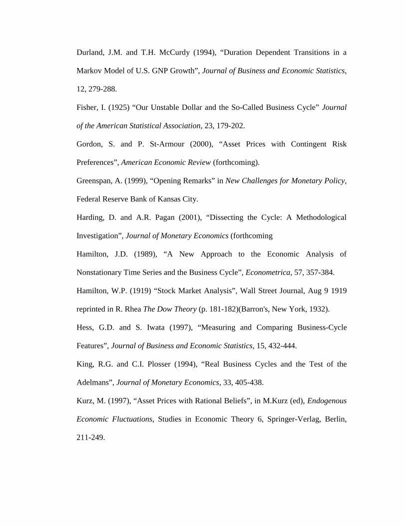
Fig 1 plots the natural log of the monthly stock price index lnPt for the U.S. over the

period 1835/1-1997/5. The series is equivalent to the S&P500 and the data sources

are given in appendix A. It is clear that there are many expansions and contractions

in the series, particularly the enormous decline in stock values during the Great

Depression.

Figure 1. Log US Stock Prices Jan 1835 – May 1997

2.00

3.00

4.00

5.00

6.00

7.00

8.00

9.00

1835

1840

1845

1850

1855

1860

1865

1870

1875

1880

1885

1890

1895

1900

1905

1910

1915

1920

1925

1930

1935

1940

1945

1950

1955

1960

1965

1970

1975

1980

1985

1990

1995

To summarize this history we apply the algorithm that incorporates the dating

methods discussed above to the series. Once we establish where the turning points

occur it is possible to summarize various characteristics of the movements between

each of these points; such expansions and contractions are termed phases. We

consider five such measures of the nature of these phases.

1. The average duration of each phase, D.

2. The average amplitude of each phase, A. For convenience, we define

“amplitude” as the difference in the logs of the stock price from one turning

point to another. This does not yield an exact measure of the actual percentage

change in the equity price over a phase owing to the fact that these movements

are sometimes large and therefore the approximation ln(1+x)=x breaks down.

3. The average cumulated movements in ln Pt over each phase, C.

4. The “shape” of the phases as measured by their departure from being a triangle.

The index used for this purpose is the “excess” index in Harding and Pagan

(2001), EX=(C-.5A-.5(A×D))/D.

5. The fraction of expansions and contractions for which A≥. 0.18 and A≤ –0.22.

These numbers translate into increases in the equity price of more than 20% and

decreases of less than 20% The motivation for considering such statistics is that

some definitions of bull and bear markets require expansions and contractions

that are of these magnitudes. We will refer to these as the B+ and B- proportions.

After defining St as a binary random variable taking the value unity if a bull market

exists at time t and zero if it is a bear market, we can estimate the quantities above

in the following way. First, the total time spent in an expansion is ∑=

T

itS

1

and the

number of peaks (hence expansions) is given by 1)1(2

1 +−= ∑=

−

T

itt SSNTP .

Therefore the average duration of an expansion will be3

.ˆ1

1∑=

−=T

ttSNTPD

The average amplitude of expansions will be

.lnˆ1

1∑=

− ∆=T

ttt PSNTPA

To get the cumulated change over any expansion we have to define

,ln1 ttttt PSZSZ ∆+= − .00 =Z Then Zt contains the running sum of ∆lnPt provided

St=1, with the sum being automatically re-set to zero whenever St=0. Hence the

total of cumulated changes over all expansions is

∑∑∑= ==

∆==T

t

t

jjj

T

tt PSZTC

1 11

ln

with the average being

.ˆ1

1∑=

−=T

ttZNTPC

All of these parameters can be found up to a factor of proportionality from

regressions e.g. C comes from the regression of Zt against unity. To get C one

needs to adjust for an incorrect scaling factor e.g. the regression coefficient in the

regression just described would need to be multiplied by .NTP

T The estimated

excess is a function of all the quantities estimated above i.e.

.ˆ/)ˆˆ5.0ˆ5.0ˆ(ˆ DDAACXE −−=

Finally, since the series (1-St)St-1 has unity at the peak of an expansion and zeros

elsewhere, while Zt contains the amplitude of each expansion at the point in time t,

the amplitudes of expansions are the non-zero values of (1-St)St-1Zt. Consequently,

],18.0)1[(1

11 >−= ∑

=−

−+T

tttt ZSSINTPB

where I[a]=1 if a is true and zero otherwise. Bear market statistics are found in the

same way by replacing St with 1-St. Since many of the statistics are non-linear

functions of sample moments we can use the δ method to compute the asymptotic

variances. Of course since A, C, D are all positive the distributions cannot be

asymptotically normal unless one is testing a null hypothesis that their expectations

have particular values.

Now the approach above is equivalent to the construction of Wald statistics for

testing hypotheses. In many ways it is more convenient to use the LM approach

since we are generally looking at whether a particular model produces statistics that

are close to those of the data. In that case we can generally do a parametric

bootstrap in order to compute p – values that reveal how close the model is to the

data.

Table 1 provides the statistics just described for the U.S. for three sample sizes. The

first uses the complete sample of observations available while the others work with

particular sub-samples used in later sections.

The statistics of Table 1 are interesting. It is clear that bull markets tend to be longer

than bear markets and the durations agree quite closely with those attributed to

Hamilton in 1921. Over time it seems as if bear markets have become shorter and

weaker while bull markets have become longer and stronger. The US stock market

also exhibits expansions and contractions that deviate quite a lot from a triangle and

this tendency has become more emphatic over time as well. The fact that there is a

departure from a triangle in the evolution of the markets is also true for the U.S.

business cycle, see Sichel (1994) and Harding and Pagan (2001). Finally, it is clear

that most expansions become bull markets as defined by their ability to rise more

than 20% while a much smaller fraction of contractions culminate in a fall in the

market of more than 20%.

As a check on the dating algorithm, Table 2 compares our results for the US to some

post-war stock market cycle dates quoted in Niemira and Klein(1994, Table 10.2,

p431) that have been used by Chauvet and Potter (1997). Their results are in

brackets. The correspondence is quite good, except for an extra contraction from

April 71 to Nov 71 (the Niermira/Klein dating stops before the last contraction

identified). There was a 10% contraction over this period and it may be that the

Niermira/Klein results incorporate some censoring based on the magnitude of

movements in share prices.

Finally, as mentioned earlier, most attention has been paid to the mean and volatility

of ∆lnPt. Slutsky (1937) and Fisher (1925) both emphasized that what seem to be

regular ups and downs in a series can simply arise from stochastic variation. Fisher

termed this phenomenon the “Monte Carlo cycle”. Malkiel (1973) noted that a

random walk in stock prices would produce cycles. Hence, as there is clearly going

to be some connection between B&B market phenomena and these two moments,

we present values for the mean µ and standard deviation σ of ∆lnPt for each of the

three samples in Table 1. These quantities are used in simulations of the next

section.

Table 3 shows that the mean capital gain has been increasing over time and the

standard deviation has been falling. However, the decline in the latter is really quite

small and statistically insignificant.

4. The Analytics of Bull and Bear Markets

To gain some appreciation of how the type of DGP determines B&B markets, return

to how initial turning points in a series were selected. A peak was taken to have

occurred at time t if the event

]ln,...,lnlnln,....,[ln 8118 ++−− ><= ttttt PPPPPPK

occurs, where Pt is the level of the stock price. One can then estimate the length of a

complete cycle by ,)Pr(

1

PK given that the number of complete cycles is one less

than the number of peaks. What a turning point rule (for a peak at t) does is to

describe the joint event (St+1=0, St=1). Now since Pr(PK) = Pr(St+1=0, St=1) we

have

).1Pr()1|0Pr()Pr( 1 ==== + ttt SSSPK

Hence it is clear that, rather than describing how a turning point occurs, we might

instead describe how one goes from the state St =1 to St+1 =0. Such a rule was

followed by Lunde and Timmermann (2000). . The difference between the two rules

resides in the need to specify Pr(St=1) i.e. in terms of dating a given realization the

need to know the initial state S0. Both methods have their attractions. The fact that

one does not need to guess at S0 means that the turning point method appeals.

However, by describing what would cause a transition between states rather than a

turning point may make it easier to take account of the magnitude of price changes

as a determinant of changes in states. To do so via the dating method one needs to

incorporate the magnitude restriction as a censoring operation as was done in one of

the steps above.

To understand the implication of the asset price DGP for bull and bear market

phenomena we concentrate upon how the DGP characteristics impact upon the

probability of the event PK occurring. Since this event depends upon the long

difference lnPt+j–lnPt , and these can be written as the sum of first differences,

{ ∆lnPt+k}jk=1, it is clear that the probability of PK will depend upon the joint

distribution of {∆lnPt+k}8k=-8 . Hence, to determine that probability one requires a

specification of the DGP for ∆lnPt. For example, if ∆lnPt was N(µ ,σ2) then the

Pr(PK) would be solely a function of µ /σ, since the turning points in lnPt are

identical to those in ln(Pt/σ). Consequently, it is likely that the probability will rise

with µ (the mean capital gain) and decline with σ. Of course, there is more to the

dating rules than that. After the initial turning points are found a set of censoring

operations is applied that will change the probability of “final” turning points.

Unfortunately, it becomes very hard to assess the precise impact of those operations

analytically and so we will be forced to resort to numerical simulation.

Nevertheless, the insight obtained from looking at what determines the initial

turning points is extremely valuable in analyzing bull and bear markets. In

particular, it is clear that, regardless of the model for ∆lnPt, the ratio of µ to σ will

be a key determinant of cycle characteristics. As an illustration of this point note

that the movements in this ratio in Table 3 are very suggestive about the actual

changes over time in bull and bear market characteristics noted in Table 1. It is clear

that any theoretical model which claims to provide an explanation of historical bull

and bear markets will also have to be capable of reproducing the historical values of

µ and σ. Since µ is related to the equity premium one must be able to replicate that

as well as the volatility of capital gains. Whether this is sufficient is something that

we investigate further in the next section.

5. Some Statistical Models of Returns

As the previous section showed it is the DGP of ∆lnPt that is the key to

understanding bull and bear markets. To this end we might categorize the potential

DGP's into those for which the capital gain is a martingale and those for which it is

not. The simplest martingale model would just be the basic random walk with drift.

,ln ttP σεµ +=∆ (1)

where εt is n.i.d.(0,1)4. Columns two and three of Table 4 provide a summary of the

bull and bear markets that would be seen in realizations of (1) when viewed through

the dating filter described earlier5. In the simulations µ=0.0042 and σ=0.0458 are

taken from the U.S. data for 1899/1-1997/5 in Table 3. It is clear that the random

walk with drift does quite well at replicating the bull and bear markets actually

observed, but the pure random walk (µ=0) fails quite badly. In fact, with the latter

we would expect symmetry in the characteristics of the phases, since the

probabilities of an initial peak and a trough occurring would be identical. The only

exception to this comes with respect to the B+ and B- statistics. There the different

censoring thresholds (-0.22 and 0.18) utilized to ensure that B&B market

movements produce a 20% movement in Pt are the sources of the asymmetries in

these proportions. If the censoring points were set to -0.2 and 0.2 then the fraction

would be 0.73 in both cases. Given this result on the importance of µ it is clear that

explaining it will be a key element in getting the nature of bull and bear markets

right. A notable deficiency with the random walk model is its implication that

phases should, on average, look like triangles, whereas this is clearly not so.

A possible extension to the basic random walk model is motivated by the fact that

(1) implies that capital gains are normally distributed, while the sample excess

kurtosis for the 1899-1997 period is 9.2. Consequently, one wants to adopt a DGP

that produces realizations for ∆lnPt from a non-normal density. One response would

be to change the density for εt to others with fatter tails e.g. Student's t, but it is more

interesting to generate the excess kurtosis “endogenously”. Some standard ways of

doing that are to treat ∆lnPt as either a GARCH(1,1) or EGARCH(1,1) process i.e. σ

in (1) is replaced by σt which varies with the past history of returns. Accordingly,

these models were fitted to US capital gains over 1889/1-1997/5 yielding:

,83.13.000087. 21

21

2−− ++= ttt e σσ

.ln95.)2

2|(|26.06.314.ln 2

1112

−−− +−+−−= tttt σπ

εεσ

In order to perform a valid comparison with the random walk model we also make

the means of the GARCH and EGARCH capital gains identical to those in the data

i.e. µ=0.0042. Columns four and five of Table 4 then process the simulated output

from the GARCH and EGARCH processes. Given the symmetry of the GARCH

process it is not surprising that it has little effect upon mean durations, but in general

it seems that the GARCH model actually does worse than the random walk. Given

that the GARCH specification produces fatter tails in the distribution of ∆lnPt it is a

somewhat surprising outcome that bull and bear markets are slightly less extreme

under it. Of course it has to be remembered that it is cumulated shocks that are

important for bull and bear markets and the GARCH model is just as likely to

produce a large positive shock as a negative one and these operate to offset one

another. The EGARCH model tends to provide a better match to most of the phase

characteristics than the GARCH model does. In particular, it is the only model that

has the ability to produce shapes of phases that resemble the data. Apart from this

last qualification the conditional volatility models don't seem to add very much to

the explanation provided by the random walk with drift model.

The above models have ∆lnPt being a martingale difference. It has long been

observed that there is little linear dependence in ∆lnPt, motivating the search for

some non-linear structure. One might fit some general non-linear models, such as

neural networks or threshold autoregressions, but in some ways it would be nicer to

be able to produce the non-linearity in a framework that preserves the flavor of the

topic being examined. Because of the emphasis being laid upon the two types of

markets, it is useful to try to obtain the requisite non-linearity by utilizing the

literature on hidden layer Markov chains. Hamilton's work (1989) is the best known

example of this in econometrics, although in other fields there have been many other

versions.

In its simplest form Hamilton's model replaces (1) with

,)()1)((ln 1100 ttttt zezeP σµσµ ++−+=∆ (2)

where zt is a random variable taking the values of zero and unity whose evolution is

governed by a Markov chain with transition probabilities p00=Pr(zt=0|zt-1=0) and

p11=Pr(zt=1|zt-1=1). Which state corresponds to which type of market is essentially

arbitrary. For the purpose of presentation and comparison of results we identify the

bull state as that which has a higher mean capital gain and label it the state

corresponding to zt=1, although we stress again this is quite arbitrary. Many

applications of Hamilton's model and its extensions have been made in the

econometric literature. Pagan and Schwert (1990) applied the basic model to US

stock returns from 1835 until 1925. Recently attempts have been made to generalize

this model to allow for the transition probabilities to depend upon the length of time

spent in a particular state i.e. to produce duration dependence. Maheu and McCurdy

(2000) is a good example. They fitted a model in which the transition probabilities

had the same format as in Durland and McCurdy (1994), namely

,)exp(1

)exp(),|Pr(

21

211

tjj

tjjttt d

ddjzjz

ψψψψ++

+=== − (3)

where dt, the duration of time spent in the j-th state in the current phase at time t, is

constrained to not exceed 16. The model they preferred was called DDMS-DD and

we took the parameters from their Table 5 to simulate it. One problem is that they fit

the model to monthly US returns rather than to capital gains. Whilst the volatility of

the returns series is much the same as capital gains since the dividend yield shows

relatively small monthly variation, the mean of returns is higher than that of capital

gains. Hence we adjusted the µ0 and µ1 parameter estimates in their model by a

scaling factor of 1.55 so that the overall mean of the simulated data agreed with that

in Table 4. By keeping the mean and variance of the simulated returns equal to that

of the data we are therefore solely studying the effect of introducing duration

dependence into the model. Data is simulated from this model in column 6 of Table

4. It provides no improvement on the results from the martingale models6.

Moreover, it fails to capture the shapes of bull and bear markets any better than the

other models. Indeed the outcomes are really rather disappointing as there is reason

for thinking that E[EX] is sensitive to duration dependence; DDMS-DD certainly

does better on this dimension than the random walk models but no better than an E-

GARCH model. Comparing the EGARCH and DDMS-DD model one is struck by

the fact that it behaves very much like a more extreme version of EGARCH

6. Some Economic Models

6.1. General Analysis

Most economic models of stock prices can be expressed as

],[1

,∑∞

=++=

j

rjttjtt

rt DIMRSEP

where Ptr=Pt/Pct is the real stock price at the end of period t, Dt

r=Dt/Pct are real

dividends paid in time t, IMRSt+j,t is the inter-temporal marginal rate of substitution

between time t and t+j and Pct is a consumption price deflator. It is useful to write

Drt+j= Dr

t(1+gt+j,t ) so that the expression for Pt has the form

=+= ∑∞

=++ ])1([

1,,

jtjttjtttt gIMRSEDP (4)

tt KD= (5)

reflecting the conditioning of the expectation upon information at time t. Then, in

real terms,

))(ln(lnlnln ttrt

rt KEKDP −∆+∆=∆ (6)

and, in nominal terms,

))(ln(lnlnln tttt KEKDP −∆+∆=∆ (7)

,ln ttD ξ∆+∆= (8)

provided ∆lnKt is a second-order stationary process. Most of the economic models

which have been advanced to explain B&B markets can be interpreted through (7),

owing to our earlier observation that the characteristics of B&B markets stem from

the nature of ∆lnPt. Effectively, these models make assumptions which determine

the processes generating ∆lnDtr, ∆lnDt and IMRSt+j,t .

To give some feel for the way in which (7) may be used, consider initially the case

that ∆lnDt ∼ N(µD, σD2), ∆lnDt

r ∼ N(µDr, σD

2r) and there is a constant discount rate.

Then IMRSt+j,t = (1/(1+r)) j and ∑

∞

= ++

=1

,)1

1(

j

jrD

t rK

µ implying that ∆lnKt=0 and the

log of capital gains will be a random walk with mean µD and volatility σD2. Moving

away from that case the mean equality remains but the volatility of ∆lnPt will now

depend upon the relative strength of the volatilities of ∆lnDt and ∆ξt. Thus economic

models will be needed whenever there is a gap between the observed moments of

the capital gains and nominal dividend growth processes. To gain some appreciation

of the likelihood of any such difference it can be noted that, over the period 1875/1-

1997/5, the ratios µ/µD and σ/σD were 1.3 and 1.03 respectively, while, over the

post-WW2 era, they become 1.12 and 2.97 respectively. Hence, to explain post-

WW2 markets one needs a substantial contribution from lnKt to the volatility of

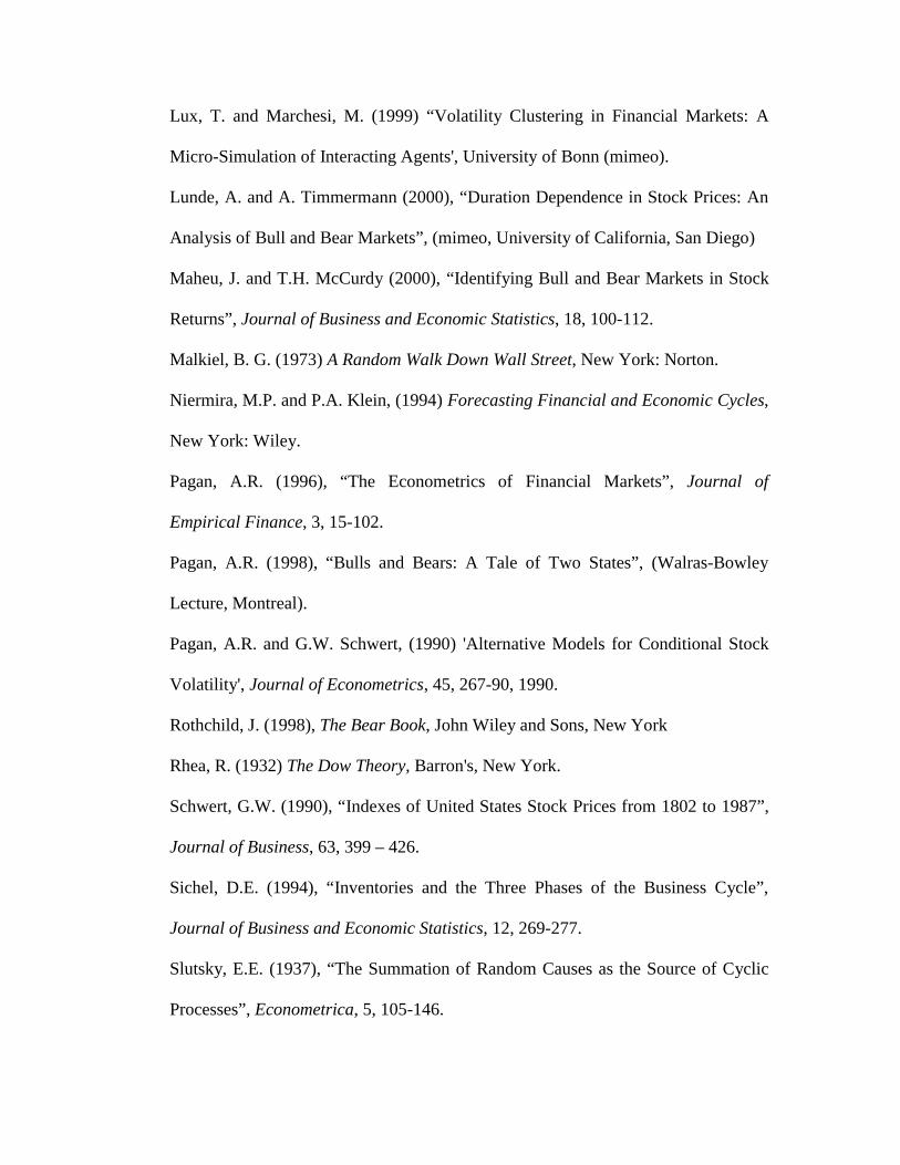
capital gains. Plots of the series show this decline in volatility in a striking way - see

fig 2. Another conclusion that can be drawn from (7) is that the nature of B&B

markets will not depend upon E(lnKt). Hence investigations that focus upon

explaining this quantity e.g. Campbell and Cochrane (1999a) are not directly

addressing B&B markets.

As mentioned above economic models tend to concentrate upon the behavior of

either the IMRS or dividends when explaining B&B phenomena, although there are

some models, notably Campbell and Kyle (1993) and Lux and Marchesi (1998),

which focus upon mechanisms involving decisions by heterogeneous agents. These

mechanisms are such as to make the price/dividend process Kt very volatile. In the

latter models equity prices are not the sum of discounted dividends, since only a

fraction of agents adhere to fundamentals in making decisions. In the next two

Figure 2. Dividend Growth from S&P Index, Jan 1875 – Dec 1995

-0.3

-0.2

-0.1

0

0.1

0.2

0.3

1875

1880

1885

1890

1895

1900

1905

1910

1915

1920

1925

1930

1935

1940

1945

1950

1955

1960

1965

1970

1975

1980

1985

1990

1995

sections we consider some economic models that focus upon the IMRS, before

moving on to dividend explanations.

6.2. The Gordon – St. Armour Model

As noted above we will be concerned here with models in which IMRSt+j,t is allowed

to follow a stochastic process. Gordon and St Armour (GSA) (2000) make it a two

state process, representing states of optimism and pessimism. In GSA the utility

function has the form γ

γ

−Θ

Θ−−

1

)( 11tC

and it is γ which can assume one of two states,

with corresponding values γ0 and γ1. Thus the aggregate IMRSt+j,t has the form

,1,0,,01

0,0,,00, tjtjtjtjtjt IMRSIMRSIMRS +++ += ψψ

where ψkl,j are probability weights determined by the transition probabilities from

state k to l (k,l=0,1) and

kltjt

jlktjt CCIMRS γγβ −−−

+−

+ ΘΘ= 1111,, )/()(

for k,l=0,1. There are some econometric issues raised by GSA's work. They assume

that Ct is an I(1) process since it comes from a VAR in differences. Since we can

write

lklttjt

jlktjt CCCIMRS γγγβ −−−

+−

+ ΘΘ= )()/( 111,,

it is clear that this makes IMRSk,lt+j,t the product of functions of an I(0) variable

Ct+j /Ct and an I(1) variable Ct. Because Ct is treated as strictly exogenous it is

unlikely that this would have any impact upon the distribution of the MLE of any

parameters of the model that are being estimated, as one can always treat it as fixed

by conditioning upon it. However, it may be that the Kt computed using IMRSt+j,t is

not I(0) and so the log of the price/dividend ratio, which equals Kt, may not be I(0)

i.e. lnPt and lnDt may not co-integrate.

Given a joint process for real dividend and consumption growth we can simulate

Gordon and St Armour's model. This produces a value for Kt. Then, as nominal

dividends follow a random walk, we can calibrate the process with values of µD and

σD used in GSA (µD=0.0048, σD=0.012), and subsequently generate simulated

values for Pt. The latter are then passed through our dating algorithm to find the

average characteristics of bull and bear markets implied by the GSA model. These

are given in Table 5 along with the actual characteristics for their estimation period.

Clearly, the model statistics are not at all like actual bull and bear markets.

Examining the simulated data it emerges that ∆lnPt has a mean and standard

deviation of 0.0047 and 0.0364 respectively, while the actual values over their data

period are 0.0051 and 0.0432, so it does not appear that the failure to match

historical B&B markets is due to a failure to get these two moments right. To check

this conclusion the last column of Table 5 examines simulated data from a process

∆lnPt ∼N(0.0047,0.0364). Comparing this column with the preceding one shows that

the strong bull and bear markets coming from the GSA model have to be due to

some difficulties with the higher order moments of ∆lnPt. Indeed, inspection of

simulated data shows that the problem seems to be that Kt jumps whenever γ

changes value and this has a profound effect upon the probabilities of getting a

turning point. It is interesting to note that, whilst µ=0.0047 and µD=0.0048 are

virtually the same (as expected), the GSA model amplifies the standard deviation

quite a lot - from σD=0.012 to σ=0.036 - a very desirable outcome.

6.3. The Campbell and Cochrane Model

Campbell and Cochrane (CC) (1999a) also produce a model that allows the IMRSt+j,t

to change over time. However, unlike the GSA solution, it now changes

continuously. Specifically they make

,)( 11,

γδ −+++ =

t

t

t

ttjt C

C

S

SIMRS

where Ct is consumption and the state lnSt evolves as a heteroskedastic

autoregressive process. To simulate data from their model they need to make some

assumptions about the parameters –δ (the risk free rate) and γ –as well as the nature

of the processes generating consumption and dividends. The logs of these latter

variables are taken to be random walks with drift. Correlation between the

innovations of the two series is allowed. The mean of the monthly real dividend

growth rate was set to that of consumption and was quantified from statistics on

consumption over 1899-1992. For this reason we will utilize data on bull and bear

markets over 1899/1-1997/5 as the benchmark to assess this model. For later

reference CC's calibration assumes that µD=0.00398 and σD=0.0388.7 CC assess

their model by its ability to replicate the equity premium, exp(E(ln(Pt/Dt)) and the

volatility of ln(Pt/Dt). Thus our experiment provides an assessment from an

alternative perspective. As we noted earlier the second of the quantities used in their

assessment methods is irrelevant to the nature of B&B markets.

Table 6 gives the results. It is apparent that the CC model captures the data quite

well and is superior to the random walk model in showing some ability to capture

the phenomenon captured by the “excess” statistic. As the CC model is known to

produce a leverage effect in volatility (something the EGARCH model was

designed to capture) this result would be expected given the outcomes in Table 4 for

the EGARCH model. In many ways its performance is reminiscent of what one gets

with the EGARCH model. Thus it seems a promising candidate for further analysis

of the nature of B&B markets.

6.4. Model Emphasizing Dividend Behavior

Another approach is to focus upon the dividend process as the cause of B&B

markets. The issue then becomes what type of process one should specify for

dividend growth. Assuming that real dividends follow a random walk of the form

,)1ln(ln trDt

rt gD εµ +=+=∆ (9)

with IMRSt+1,t=(1+r)-1, then Kt=[1-r×exp(µDr+½σε

2)]-1, provided

r×exp(µDr+½σε

2)<1. Thus the price-dividend ratio becomes a constant which

depends on the volatility of dividend growth as well as its mean. To make Kt

stochastic therefore requires a more complicated process than (9) for real dividend

growth. A simple way of introducing some stochastic variation into Kt is to allow εt

to be a GARCH process. Then Kt will depend on a discounted sum of all the higher

order conditional moments. This extension is problematic since the forecast of a

conditional moment normally converges to the unconditional one as the forecast

horizon lengthens, but very few unconditional moments exist for GARCH

processes, so it may be very unlikely that the sum in (4) actually converges i.e. Kt

may have no moments.

Another way to induce some stochastic variation into Kt is to allow for some serial

correlation in ln(1+gt) i.e. the model for dividend growth becomes

.))1(ln()1ln(ln 1 trDt

rDt

rt ggD εµφµ +−++=+=∆ −

Then one might attempt to evaluate (4) with this specification. This is quite difficult

since ∏=

++ +=+j

kktjjt gg

1, )1(1 and so

,)1(1 1

∑ ∏∞

= =++=

k

k

iitt

kt gEK β

where β=IMRSt+1,t. If εt is N(0,σε2) then ∏

=++ +=+

k

jjtkkt gg

1, )1(1 is log-normal with

ln (1+gt+k,k) having moments

),)1(ln(1

)1( rDt

krDk gk µ

φφφµµ −+

−−+=

).1

1

1

12(

)1( 2

22

2

22

φφφ

φφφ

φσσ ε

−−+

−−−

−=

kk

k k

Therefore

]2

1))1(log(

1

)1(exp[)1( 2

1υσµ

φφφµ +−+

−−+=+∏

=+

rDt

krD

k

iitt gkgE

and

,)))1(21

(exp()))1(2

exp([()exp

1( )()(

2

2

2

2

2

2

1

1 22 φφεεφφ

φσ

φφ

φσ

µβµ

BAg

Kkkr

Dk

rD

tt −−

−−

++

= ∑∞

=

−

where

)),)1)1(2

)()1(2

exp(2

2

2

2

φφ

φφ

φσ ε

−−

−−=A

.)1

exp)(

)1(1exp( 1

2

2φ

φε µφ

σφ

φ −

+−−=

t

rD

gB

Kt is an infinite sum of different powers of a single lognormal variable. However,

the term exp(µDr/(1+gt))

φ/(1-φ) in B makes it hard to find the exact value of Kt. If,

however, the sum is approximated by setting B=1 then

,)1( 1 φφ−+= tt gCK

and so the price-dividend ratio is stochastic and depends upon the growth rate of

dividends at the point that the expectation is being taken.8 Moreover, as φ rises i.e.

the degree of persistence of shocks into the dividend growth rate increases, Kt will

rise.

Given the formula above for Kt and using the relation between real equity prices and

real dividends in (6) it follows that

,)1(ln 1t

rD

rtP εφµ −−+=∆

Now, we might expect that volatility in nominal and real equity prices are much the

same due to stickiness in consumer prices, so that ∆lnPt will be well approximated

by N(µD, (σ/(1-φ))2). Thus the introduction of serial correlation into the dividend

process amplifies the volatility of equity prices and 2

)lnvar(

D

tP

σ∆

will be φφ

−+

1

1. This

latter effect produces a dilemma for an investigator. By increasing φ it is possible to

realize much larger values of lnKt and thereby increase the magnitude of realizations

of lnPt. But the rise in volatility in ∆lnPtr also means that the average bull market

becomes shorter and of smaller amplitude. Thus the explanation of a particular

episode may compromise the ability to explain average market outcomes. Some

amplification of volatility is desirable however since there is not enough volatility in

dividend growth itself to explain the volatility in stock prices. As we observed

earlier the ratio of σ to σD for post-war data is around 3, so that a value of φ=0.8

would be needed to produce the correct volatility in capital gains, given the

observed dividend volatility. This is quite a high degree of persistence and, although

it is smaller than that used by Barsky and de Long (1993), it is subject to the same

criticism that has been made of their argument.

6.5. Studying Extreme Events

The history of asset price movements is replete with instances of extreme behavior

e.g. the movement in equity prices in the US during the 1920s. Extreme events in

asset markets are interesting for a number of reasons. One is that they provide a very

demanding test of any postulated model. Another is that they are frequently used to

shed light on the importance of bubbles within these markets. The latter motivation

has produced several papers which have enquired into the nature of the bull and bear

markets of the 1920s. Donaldson and Kamstra (1996) is probably the best known of

these. They argued that the high price-dividend ratios of the 1920s were a

consequence of the dividend processes at that time. To establish this fact they fit

models to t

tt

r

gy

++

=1

1, where rt is an interest rate on low-risk commercial paper

plus a constant equity premium and ∑∏∞

= =+=

1 1

][j

j

kkttt yEK . The models have the form

,)1()1)(1( 12

212

21 ttt uLLayLLL +−−+=−−− −ψρρβρρ (10)

where ψt-1 is a non-linear function of past yt and ut has a GARCH structure. They

recursively estimate the parameters of this process.

Since the objective is to find a large value of Kt during the 1920s bull market, we

might begin by examining the degree of persistence in the yt process. Ignoring the

non-linearity in (10), persistence could be measured by the roots of the equation

(1-ρ1L-ρ2L2)(1-βL)=0 and, from their Table 3, these roots are very close to unity

(the dominant root is 1.02 using estimates over samples from 1899/1 up to 1919/12

and 1925/12). Consequently, although the analysis of the previous section had ln(1+

gt) rather than yt evolving as an AR(1) structure, we might expect that the result

found there would still hold i.e. the strong persistence has the potential for

producing a large value of K. One of their simulations (reported in their figure 4)

effectively sets φ=0.97 and such an outcome can indeed be observed. Of course this

was Barsky and de Long's point and the question which arose in comment on their

paper was what the evidence was for such persistence in dividend growth. Yearly

real dividend growth does not show any. Monthly dividends are harder to analyze

owing to their seasonality and occasional very large spikes. Donaldson and Kamstra

removed these effects by performing seasonal adjustment with the X-11 program

followed by smoothing operations to eliminate spikes in the series. It is this adjusted

series that become yt. Thus there has to be a question mark over the origin of the

persistence they find. It should also be noted that Donaldson and Kamstra maintain

that the non-linearity and GARCH effects in (10) are very important to getting a

large enough Kt. We find it hard to evaluate this argument since they compute Kt by

simulation methods and so it is necessary to assume that all moments of this random

variable exist, and we have already pointed out that this is problematic with

GARCH structures.

We turn to another way of looking at the issue of whether the 1920s can be

explained by fundamentals, asking whether a particular model is capable of

generating outcomes such as occurred at that period in time i.e. rather than

focussing upon the average B&B market characteristics as in earlier sections we

look at the likelihood of extreme movements being generated by a particular model.

Let us concentrate first on bull markets. Because we have a method for demarcating

the periods of a bull market it is possible for us to simulate from a given process for

equity prices and then determine whether any observed movement in a bull market

is likely to have come from the assumed process. The computation is like that used

in value at risk analysis.

A number of questions might then be asked. First, was the amplitude and the

duration of the 1920s bull market unusual? Second, was the particular conjunction

of those two characteristics observed at that time unusual? Essentially this analysis

asks whether it was possible for there to be a sequence of dividend outcomes and a

realization of Kt which supports a bull market defined with a specific amplitude and

duration. It differs from Donaldson and Kamstra's work in that it does not directly

address whether the actual dividends and likely value of Kt during the 1920s were

such as to produce the necessary outcome for Kt.

To examine the first of these questions we select a model to simulate from and then

summarize the history of amplitudes and durations of bull and bear markets from a

long simulation. We have produced 3000 bull and bear markets in this way by

simulating a random walk model with the µ and σ values from 1835/1-1997/5. Fig 3

cross plots the amplitudes against the durations of the bull markets; also marked on

this graph is the 1920's configuration.

It is clear that the 1920s bull market is not an improbable event when equity prices

evolve as a random walk with the historical µ and σ. Another way to compare

model output and data is to fit a linear relation between the amplitudes and the

durations from the simulated data and to then place that relation on a similar graph

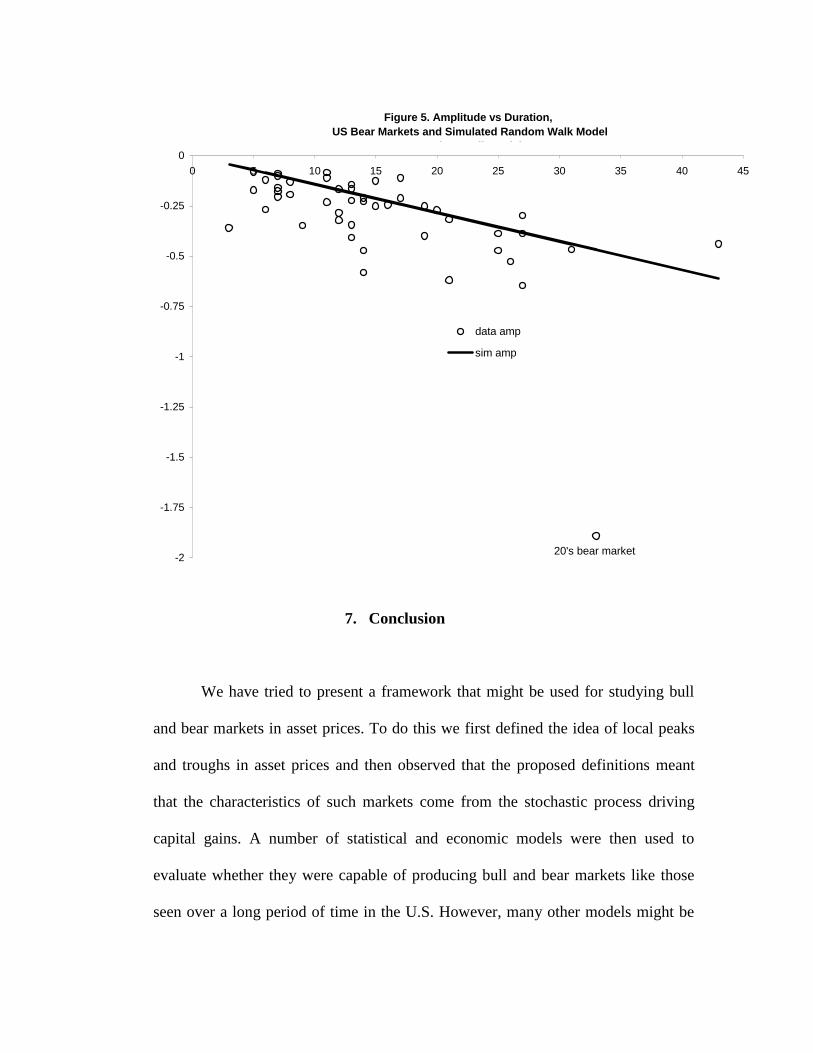
to fig 3, along with historical bull market characteristics. Figure 4 does this and it

shows that the random walk is quite a satisfactory model for bull markets. Its main

deficiency is the inability to explain some long bull markets that failed to produce a

large rise in stock prices. Fig 5 is the equivalent of fig 4 for bear markets and it is

Figure 3. Amplitudes vs Durations of Bull Markets from Simulated Random Walk Mode l

-0.2

0.3

0.8

1.3

1.8

2.3

0 20 40 60 80 100 120 140 160

X

``

X - 20's bull market

equally clear that the bear market at the end of the 1920s would never have been

predicted by the random walk model. Thus, even though this model is capable of

producing quite large declines in share prices, they only come with long duration

bear markets and this one was quite short.9

0

0.25

0.5

0.75

1

1.25

0 10 20 30 40 50 60 70 80

data ampsim amp

Figure 4. Amplitudes vs Durations, US Bull Markets and Simulated Random Walk Model

R d W lk M d l 20's bull market

7. Conclusion

We have tried to present a framework that might be used for studying bull

and bear markets in asset prices. To do this we first defined the idea of local peaks

and troughs in asset prices and then observed that the proposed definitions meant

that the characteristics of such markets come from the stochastic process driving

capital gains. A number of statistical and economic models were then used to

evaluate whether they were capable of producing bull and bear markets like those

seen over a long period of time in the U.S. However, many other models might be

-2

-1.75

-1.5

-1.25

-1

-0.75

-0.5

-0.25

0

0 5 10 15 20 25 30 35 40 45

data amp

sim amp

Figure 5. Amplitude vs Duration, US Bear Markets and Simulated Random Walk Model

R d W lk M d l

20's bear market

used to generate a process for capital gains, realizations of which may be fed into

our dating process, thereby enabling us to directly study the factors which give rise

to bull and bear markets. For example, VAR models have sometimes been proposed

that have asset prices as one of the variables within the system so that it would be

possible to study which of the shocks that drive the VAR are responsible for bull

and bear markets.

Appendix A. Stock Market Data

The US data is over 1835/1-1997/5 and consists of combining series from Schwert

(1990) from 1835/1-1870/12 and the S&P index thereafter. From 1871/1-1956/12

this data was taken from series 11011 in the NBER macroeconomic database.

Missing observations in 1914 due to the closure of the NYSE at the outbreak of

WW1 were linearly interpolated. Dividends are those derived from a comparison of

the S&P index with and without dividends and were obtained from Allan

Timmerman.

Appendix B. Procedure for Programmed Determination of Turning Points.

1. Determination of initial turning points in raw data.

A. Determination of initial turning points in raw data by choosing local peaks

(troughs) as occurring when they are the highest (lowest) values in a window

eight months on either side of the date.

B. Enforcement of alternation of turns by selecting highest of multiple peaks

(or lowest of multiple troughs).

2. Censoring operations (ensure alternation after each).

A. Elimination of turns within 6 months of beginning and end of series.

B. Elimination of peaks (or troughs) at both ends of series which are lower or

higher).

C. Elimination of cycles whose duration is less than 16 months.

D. Elimination of phases whose duration is less than 4 months (unless fall/rise

exceeds 20%).

3. Statement of final turning points

Table 1. Statistics on Bull and Bear Markets in US Stock Price Data*

1835/1-1997/5 1889/1-1997/5 1945/1-1997/5

Bear Duration 16 14 12

Bull Duration 25 25 26

Bear Amplitude -0.32 -0.32 -0.24

Bull Amplitude 0.43 0.45 0.46

Bear Cumulated -2.72 -2.66 -1.60

Bull Cumulated 7.28 7.71 7.70

Bear Excess 0.025 0.022 0.016

Bull Excess 0.019 0.026 0.030

B- 0.61 0.53 0.40

B+ 0.83 0.88 0.93

*Amplitudes are % changes, durations are in months.

Table 2. Post-War US Stock Market Cycles: Two Dating Methods

(Niermira/Klein in brackets)

Peak Trough

1946/5 (1946/4) 1948/2 (1948/2)

1948/6 (1948/6) 1949/6 (1949/6)

1952/12 (1953/1) 1953/8 (1953/9)

1956/7 (1956/7) 1957/12 (1957/12)

1959/7 (1959/7) 1960/10 (1960/10)

1961/12 (1961/12) 1962/6 (1962/6)

1966/1 (1966/1) 1966/9 (1966/10)

1968/11 (1968/12) 1970/6 (1970/6)

1971/4 1971/11

1972/12 (1973/1) 1974/9 (1974/12)

1976/12 (1976/9) 1978/2 (1978/3)

1980/11 (1980/11) 1982/7 (1982/7)

1983/6 (1983/10) 1984/5 (1984/7)

1987/8 (1987/9) 1987/11 (1987/12)

1990/5 (1990/6) 1990/10 (1990/10)

1994/1 1994/6

Table 3. Mean and Standard Deviation of Capital Gains

1835/1 – 1997/5 1889/1 – 1997/5 1945/1 – 1997/5

µ 0.0031 0.0042 0.0066

σ 0.044 0.0458 0.0404

µ/σ 0.07 0.09 0.16

Table 4. US Bull and Bear Markets Generated by Various Statistical Models*

Data RW

µ=0

RW

µ≠0

GARCH

µ≠0

EGARCH

µ≠0

DDMS-DD

Dur Bear 15 20 16 15 15 15

Dur Bull 26 20 25 26 26 27

Amp Bear -0.31 -0.34 -0.27 -0.26 -0.30 -0.28

Amp Bull 0.45 0.34 0.44 0.43 0.47 0.48

Cum Bear -2.71 -4.46 -2.70 -2.53 -2.87 -2.64

Cum Bull 7.84 4.46 7.65 7.71 8.92 9.67

Ex Bear 0.020 -0.000 -0.000 -0.000 0.005 0.005

Ex Bull 0.024 0.000 0.000 0.000 0.011 0.008

B- 0.51 0.70 0.58 0.49 0.56 0.49

B+ 0.86 0.76 0.85 0.81 0.86 0.82


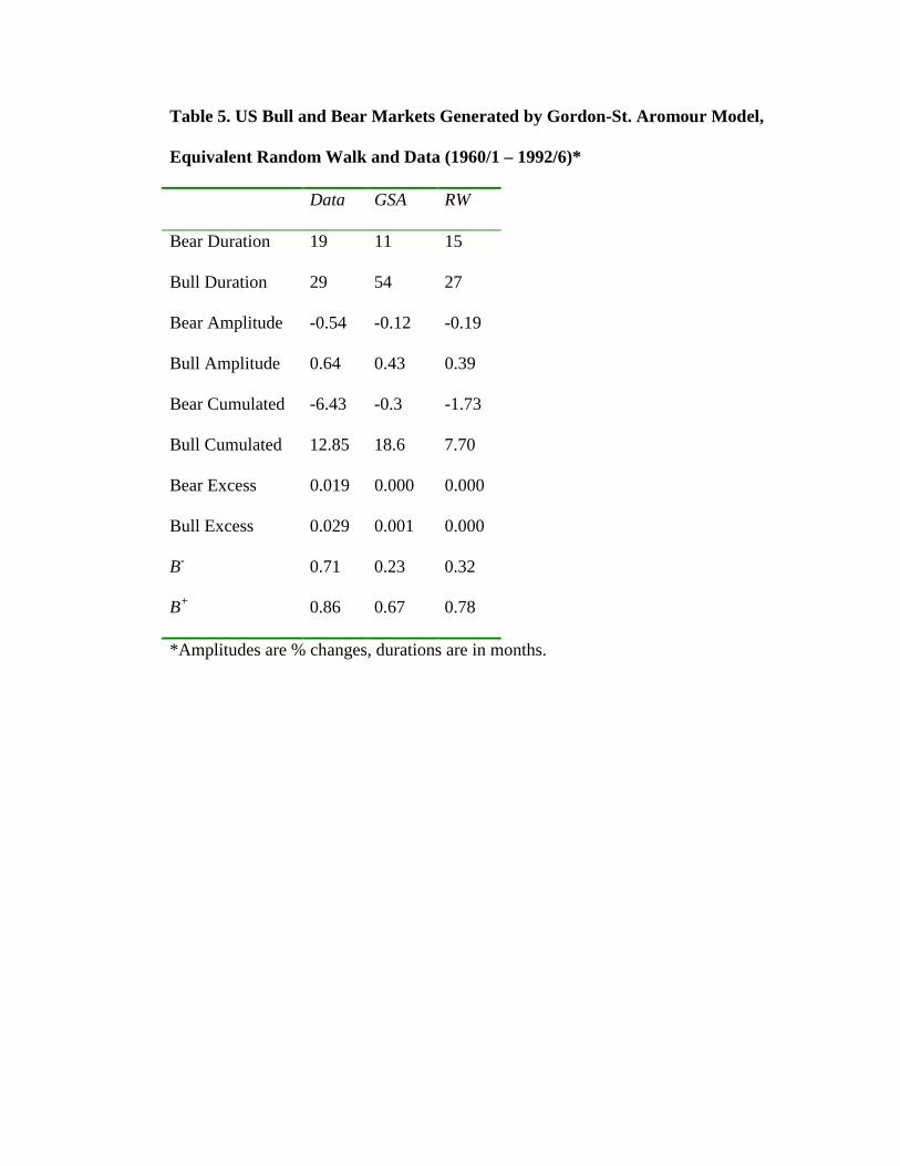
Table 5. US Bull and Bear Markets Generated by Gordon-St. Aromour Model,

Equivalent Random Walk and Data (1960/1 – 1992/6)*

Data GSA RW







Bear Excess 0.019 0.000 0.000

Bull Excess 0.029 0.001 0.000

B- 0.71 0.23 0.32

B+ 0.86 0.67 0.78


Table 6. US Bull and Bear Markets Generated by Campbell-Cochrane Model,

Equivalent Random Walk and Data (1899/1 – 1997/5)*

Data GSA RW







Bear Excess 0.022 0.006 0.000

Bull Excess 0.026 0.009 0.000

B- 0.51 0.67 0.58

B+ 0.86 0.89 0.85


References

Barsky, R. and B. de Long (1993), “Why does the Stock Market Fluctuate?”,

Quarterly Journal of Economics, 108, 291-311.

Bernanke, B. and M. Gertler (1999), “Monetary Policy and Asset Price Volatility”,

in New Challenges for Monetary Policy, Federal Reserve Bank of Kansas City.

Bry, G. and C. Boschan (1971), Cyclical Analysis of Time Series: Selected

Procedures and Computer Programs, New York, NBER.

Campbell, J.Y. and A.S. Kyle (1993), “Smart Money, Noise Trading and Stock

Price Behaviour”, Review of Economic Studies, 60, 1-34.

Campbell, J.Y. and J.H. Cochrane (1999a),”By Force of Habit: A Consumption-

Based Explanation of Aggregate Stock Market Behavior”, Journal of Political

Economy, 107, 205-251.

Campbell, J.Y. and J.H. Cochrane (1999b), “Explaining the Poor Performance of

Consumption-Based Asset Pricing Models” (mimeo, University of Chicago).

Campbell, J.Y. A.W. Lo and A.C. MacKinlay (1997), The Econometrics of

Financial Markets (Princeton University Press, Princeton).

Chauvet, M. and S. Potter (2000), “Coincident and Leading Indicators of the Stock

Market”, Journal of Empirical Finance, 7, 87-111.

Donaldson, R.G. and M. Kamstra (1996), “A New Dividend Forecasting Procedure

that Rejects Bubbles in Asset Prices: The Case of the 1929's Stock Market Crash”,

Review of Financial Studies, 9, 333-383.

Durland, J.M. and T.H. McCurdy (1994), “Duration Dependent Transitions in a

Markov Model of U.S. GNP Growth”, Journal of Business and Economic Statistics,

12, 279-288.

Fisher, I. (1925) “Our Unstable Dollar and the So-Called Business Cycle” Journal

of the American Statistical Association, 23, 179-202.

Gordon, S. and P. St-Armour (2000), “Asset Prices with Contingent Risk

Preferences”, American Economic Review (forthcoming).

Greenspan, A. (1999), “Opening Remarks” in New Challenges for Monetary Policy,

Federal Reserve Bank of Kansas City.

Harding, D. and A.R. Pagan (2001), “Dissecting the Cycle: A Methodological

Investigation”, Journal of Monetary Economics (forthcoming

Hamilton, J.D. (1989), “A New Approach to the Economic Analysis of

Nonstationary Time Series and the Business Cycle”, Econometrica, 57, 357-384.

Hamilton, W.P. (1919) “Stock Market Analysis”, Wall Street Journal, Aug 9 1919

reprinted in R. Rhea The Dow Theory (p. 181-182)(Barron's, New York, 1932).

Hess, G.D. and S. Iwata (1997), “Measuring and Comparing Business-Cycle

Features”, Journal of Business and Economic Statistics, 15, 432-444.

King, R.G. and C.I. Plosser (1994), “Real Business Cycles and the Test of the

Adelmans”, Journal of Monetary Economics, 33, 405-438.

Kurz, M. (1997), “Asset Prices with Rational Beliefs”, in M.Kurz (ed), Endogenous

Economic Fluctuations, Studies in Economic Theory 6, Springer-Verlag, Berlin,

211-249.

Lux, T. and Marchesi, M. (1999) “Volatility Clustering in Financial Markets: A

Micro-Simulation of Interacting Agents', University of Bonn (mimeo).

Lunde, A. and A. Timmermann (2000), “Duration Dependence in Stock Prices: An

Analysis of Bull and Bear Markets”, (mimeo, University of California, San Diego)

Maheu, J. and T.H. McCurdy (2000), “Identifying Bull and Bear Markets in Stock

Returns”, Journal of Business and Economic Statistics, 18, 100-112.

Malkiel, B. G. (1973) A Random Walk Down Wall Street, New York: Norton.

Niermira, M.P. and P.A. Klein, (1994) Forecasting Financial and Economic Cycles,

New York: Wiley.

Pagan, A.R. (1996), “The Econometrics of Financial Markets”, Journal of

Empirical Finance, 3, 15-102.

Pagan, A.R. (1998), “Bulls and Bears: A Tale of Two States”, (Walras-Bowley

Lecture, Montreal).

Pagan, A.R. and G.W. Schwert, (1990) 'Alternative Models for Conditional Stock

Volatility', Journal of Econometrics, 45, 267-90, 1990.

Rothchild, J. (1998), The Bear Book, John Wiley and Sons, New York

Rhea, R. (1932) The Dow Theory, Barron's, New York.

Schwert, G.W. (1990), “Indexes of United States Stock Prices from 1802 to 1987”,

Journal of Business, 63, 399 – 426.

Sichel, D.E. (1994), “Inventories and the Three Phases of the Business Cycle”,

Journal of Business and Economic Statistics, 12, 269-277.

Slutsky, E.E. (1937), “The Summation of Random Causes as the Source of Cyclic

Processes”, Econometrica, 5, 105-146.

Timmermann, A. (1996), “Excess Volatility and Predictability of Stock Prices in

Autoregressive Dividend Models with Learning”, Review of Economic Studies, 523-

557.

Watson, M. (1994), “Business Cycle Durations and Postwar Stabilization of the

U.S. Economy”, American Economic Review, 84,24-46.

1 Pagan (1998) does this exercise for two other countries, the U.K. and Australia. There are manysimilarities to the US in the types of markets for these countries but, because most theoretical modelshave been calibrated to U.S. data, we focus on it in the current paper.2 It might be thought that the minimum phase length would be eight months since that would be animplication of the rule used to get the initial dates but later we allow a deviation from normal phaselengths based on quantitative movements in the stock price index.3Some difficulties arise due to incomplete phases at the both ends of the sample. Since we actuallymeasure the features of completed phases the summation should run from the beginning of the firstcompleted phase until the end of the last one rather than over 1,...,T. Since the asymptotics is notaffected by that modification we use the complete sum in these formulae.4 Strictly speaking this is not a martingale unless one removes the drift but we will keep theterminology.5 Our frame of reference for discriminating between models is the ''cycle information''. Of course (1),with values of µ and σ from Table 3, can almost certainly be rejected as failing to replicate otherfeatures of the data. The simplest would just be the magnitude of ∆lnPt in any month. Since threestandard deviations from the mean is an implausible outcome for ∆lnPt, using US estimates of µ andσ over 1835/1-1997/5 would imply that a value of ∆lnPt less than -.127 (a 12.7% contraction) shouldrarely come up, whereas it actually occurs about 1% of the time in the US data.6 Although it should be noted that Maheu and McCurdy estimated the model with data from 1835 andnot 1899.7 We used a program available on John Cochrane's web page to generate the data. The value CCassigned to µD

r comes from per capita real consumption data and to get µ D this needs to be inflatedwith the rate of price inflation. Using the PPI yearly inflation rate over 1899-1997 as a deflator, thelatter adds 0.0024 to their µD

r =0.00158.8 Because µD and gt are monthly values it is likely that B will be very close to unity even for quitehigh values of φ. For example if µD

r=0.004, gt=0.006, φ =0.8 then B=0.992.9 It is worth remembering that we use local turning points to demarcate the phases. Although therewas a strong recovery from the trough in June 1932 to a peak in February 1934, the level had notreturned to the peak of the 1920's. The market had essentially only recovered to its level of 1924.

A Simple Framework for Analyzing Bull and Bear Markets

Documents

Transcript of A Simple Framework for Analyzing Bull and Bear Markets