A Review of the Energy Productivity Center's"Least-Cost Energy Strategy" Study

by

David 0. WoodMichael ManoveErnst R. Berndt

June 30, 1981(Revised November 30, 1981)

MIT Energy Laboratory Report No. MIT-EL 81-043

A Review of the Energy Productivity Center's"Least-Cost Energy Strategy" Study

MASSACHUSETTS INSTITUTE OF TECHNOLOGY

Energy LaboratoryEnergy Model Analysis Program

by

David 0. WoodMichael ManoveErnst R. Berndt

Contributors

Alan CoxRonald KrummEdward Mensah

Eric ShumabukuroGeorge Tolley

Prepared for:

Electric Power Research Institute3412 Hillview Avenue

Palo Alto, California 94304

EPRI Project Manager:

Richard RichelsEnergy Analysis and Environment Division

NOTICE

This report was prepared by the organization(s) named below as an accountof work sponsored by the Electric Power Research Institute, Inc. (EPRI).Neither EPRI, members of EPRI, the organization(s) named below, nor anyperson acting on their behalf: (a) makes any warranty or representation,express or implied, with respect to the accuracy, completeness, orusefulness of the information contained in this report, or that the useof any information, apparatus, method, or process disclosed in thisreport may not infringe privately owned rights; or (b) assumes anyliabilities with respect to the use of, or for damages resulting from theuse of, any information, apparatus, method, or process disclosed in thisreport.

Prepared by

Massachusetts Institute of TechnologyCambridge, Massachusetts 02139

-i-

ACKNOWLEDGEMENTS

Contributions from several individuals must be mentioned. At anearly stage of this review Steve Carhart of the Mellon Institute's EnergyProductivity Center (EPC) provided a comprehensive'briefing on theobjectives and organization of EPC's "Least-Cost Energy Strategy" Study,and transmitted to us the materials which comprise the documentation forthis review. Later he commented on the first draft of this report.

The organizations responsible for the models used in EPC's studyalso provided valuable assistance in completing the model descriptionquestionaires included in Appendix A. In particular we acknowledge theassistance of Samir Salama and Harold Kalkstein of Energy andEnvironmental Analysis, Inc.; Michael Lawrence of Jack FaucettAssociates; and Peter T. Kleeman of the Brookhaven National Laboratory.Roger Bohn of the MIT Sloan School also "consulted" with us regarding theISTUM model, a modeling effort in which he participated at an earlierstage as an employee of Energy and Environmental analysis, Inc.

We wish to acknowledge helpful comments from Rene Males of EPRI,Paul Joskow of MIT, David Strom of the Office of Technology Assessment,Alan Meier of the University of California at Berkeley, and Roger Bohn.

Finally we acknowledge the support provided by EPRI in organizingand conducting this review. We have benefited from several conversationswith Larry Williams of the EPRI Demand Analysis group. As in previousEMAP studies, Richard Richels has contributed significantly to both theorganization and content of the study.

-ii-

EXECUTIVE SUMMARY

The Mellon Institute's Energy Productivity Center (EPC) has recentlycompleted a study asking the question, "How would the nation haveprovided energy services in 1978 if its capital stock had eenreconfigured to be optimal for actual 1978 energy prices?" Interestin this question is motivated by the unanticipated increases in oilprices since 1973. If policy makers are to learn from history it isimportant to know what would have happened if the increases in energyprices had been foreseen and if the nation had taken full advantage ofthat knowledge to minimize costs.

EPC concludes that if the 1978 capital stock had been transformed inconformance with a least-cost principal for providing energy services,then, given actual 1978 energy prices and energy service demands, percapita energy service costs would have been reduced by 17%. Marketshares of the various energy types would also have been affectedsubstantially. For example, while the gas share of total energy servicedemand would have increased slightly from actual 1978 levels, the shareof purchased electricity would have fallen from 30% to 17% of totalenergy service demand, and improvements in energy efficiency would haveincreased from 10% to 32%.

EPC's findings have received considerable attention, both from thepress and from policy makers. EPC interprets its results as indicating"... the direction in which we coul move to begin realizing some of thebenefits of a least-cost strategy."

The purpose of this report is to assess and evaluate the EPCmethodology, data base, and results. Here we briefly summarize ourprincipal findings.

SUMMARY OF FINDINGS

1. The Energy Productivity Center's retrospective, "Least-Cost EnergyStrategy" (LCES) study is provocative regarding the potential roleof efficiency technologies in competition with energy supplytechnologies. Their decision to conduct a "what if' analysis for arecent year provides an historical context for interpreting andreviewing the results.

1.1 As a result of its predication on known prices andtechnologies, the question posed by EPC avoids analysis of thedifficult problems of uncertainty, shocks, and other"surprises," and instead focuses on the issue of optimaladjustment to higher energy prices.

-iii-

1.2 The retrospective vantage of the LCES study helps us learn fromhistory and has implications for optimal adjustment to futureenergy-price increases.

2. The LCES study is subtitled: "Minimizing Consumer Costs ThroughCompetition." But the effects of competition are not explored inthe body of the study. All of EPC's analysis is devoted toconstructing a hypothetical optimal strategy and comparing thatstrategy to what actually occurred. EPC suggests, withoutsubstantiation, that competiton would cause an optimal strategy tomaterialize. It should be kept in mind that many economists,planners and regulators would argue that an optimal strategy can beimplemented only with planning and regulation.

3. The methodology chosen by EPC to construct an optimal energystrategy is based on the least-cost energy-strategy (LCES)objective. This methodology has several advantages over otherconventional policy objectives.

3.1 Because of its general nature the least-cost objective functioncan simultaneously take account of many different kinds ofissues. Matters such as resource limitations, environmentalfactors and national security can all be evaluated and comparedwithin the framework of the least-cost method. This way offormulating policy is far more appealing than a method thattakes account of only one significant issue (such as energyindependence).

3.2 Because costs must be quantified before they can be minimized,the least-cost method invites the analyst to use hard data whenit is available. Vague judgments are thus discouraged.

4. Least-cost methodology is limited for several reasons, and it yieldsresults which tend to overstate -- perhaps substantially -- theeconomic desirability of energy-efficiency improvements. Hence LCESimplications for policy in this area may be misleading.

4.1 There are many potential market responses to new energy priceconditions:

i. Consumers may substitute less energy-intensive consumergoods for more energy-intensive consumer goods.

ii. Producers may substitute less energy-intensive inputs formore energy-intensive inputs in the production of a broadspectrum of commodities.

iii. Producers may substitute more energy-efficient processesfor less energy-efficient processes in the production ofenergy services.

- - ---- . -------- - -* I mh IIIIIYIIYm m I i.mr In~

-iv-

iv. Secondary price changes may occur for many fuels and otherenergy rich commodities.

The least-cost methodology as applied by EPC takes account ofonly one of these market responses, namely, iii. above.

4.2 Least-cost methodology does not treat the level of benefits asa subject of consumer choice. Costs are permitted to vary as afunction of the energy-service technologies selected, but theoutput of goods, and thus consumer benefits, are exogenouslyfixed. That is why the least-cost method cannot allowconsumers to substitute less energy-intensive consumer goodsfor more energy-intensive consumer goods (e.g. i., above).

4.3 In contrast, the methodology of maximizing net benefitssimultaneously chooses the appropriate bundle of outputs andthe least-cost strategy for attaining that bundle. Maximizingnet benefits and minimizing costs are equivalent only underrestrictive and unlikely conditions. This raises importantquestions about the use of least-cost strategies for public andprivate policy formation.

4.4 When net-benefits maximization replaces cost-minimization asthe policy objective, the indicated optimal improvement in theenergy efficiency of capital goods is reduced. The interactionbetween the demand for services, capacity utilization and theoptimal energy-efficiency of capital is an essentialconsideration in adjusting to higher energy prices. Ignoringthis interaction biases LCES results toward excess efficiency.Some preliminary analysis suggests this bias may be substantial.

4.5 LCES strategies are deficient in that they recognize only thecosts of energy-service inputs in the production of non-energygoods. They do not analyze the cost of other inputs tonon-energy goods production, e.g. labor, capital, environmentalconditions, non-energy materials, and primary resources. As aresult, the LCES method cannot be used to analyze thesubstitution of less energy-intensive inputs for moreenergy-intensive inputs in general productive processes (e.g.ii., above). This omission further biases LCES results towardsexcess efficiency.

5. In constructing the LCES model, EPC described technologies for theproduction of energy services in great detail.

5.1 This detail is potentially useful in drawing conclusions aboutthe future role of specific technologies in the production ofenergy services. EPC has advanced the state of the art ofmodelling energy-services production by integrating detailedinformation concerning a wide variety of energy services.

5.2 However, because of lack of attention to some of the broaderissues discussed above, many of the detailed LCES results maybe artifacts of methodology. Therefore, we believe it wouldhave been more fruitful to distribute modelling resources moreevenly among the issues listed under 4.1, to trade off detailfor broader scope and a more appealing objective than leastcost.

6. The EPC retrospective question can be stated succinctly: "How wouldthe nation have provided energy services in 1978 if its capitalstock had been reconfigured to be optimal for actual 1978 energyprices." .We believe that the focus of this question is toorestricted.

6.1 In fact, only a part of the capital stock is permitted toadjust. The least-cost strategy implicitly gives the gift ofperfect foresight to end-use consumers of energy services butnot to other decision makers, so that the least-cost strategyis a partial optimization.

6.2 Using actual energy prices rather than estimates of marketprices greatly restricts the interpretation of the LCES studyresults as optimal. Further, the use of such prices, whichinclude distortions due to regulation and market failures, isinconsistent with the spirit of a paper purporting todemonstrate the advantages of increased competition. Wesuggest that EPC should have used imputed free-market pricesrather than "actual 1978 energy price."

7. We suggest an alternative retrospective question: "How would thenation have provided energy services in 1978 if cost-minimizingeconomic decision makers with perfect foresight had defined thedomestic economic environment, constrained only by the domesticenergy endowment and by world-market prices of energy resourcesabroad?" The answer to this question would be substantiallydifferent from the answer to the question posed by EPC, and, wethink, more interesting.

7.1 With universal perfect foresight, public policies in the 1960'sand 70's might well have mitigated the disruptive economicconsequences of energy price shocks. A more fully adjustedmacro-economy with greater economic growth and fewer recessionsmight have resulted.

7.2 With universal perfect foresight, investment levels andpatterns of the energy-production, conversion, transportationand distribution industries would have been very different fromtheir actual 1978 realization. For example, the electric powerindustry--with its long-lived capital and investment leadtimes--would have obtained a smaller and "optimally reconfigured"1978 capital stock, resulting in lower electricity prices.

-V-

-vi-

7.3 Governmental policy that allowed the deregulation of all fuelin the U.S. might have led to more rational fuel use and fewershortages, as well as different energy service demand andprices in 1978

7.4 EPC argues that its optimization methodology is satisfactoryfor indicating "..the direction in which we could move to beginrealizing some of the benefits of a least-cost strategy." Buteven the direction of change indicated by a partialoptimization process may differ from the direction indicated bya complete optimization. Many of the opportunities forreducing the costs of energy services identified by LCES coulddisappear when the range of possible adaptations areincreased.

8. LCES treats 1978 fuel prices as exogenous to the least-coststrategy. As a result, the fuel prices EPC uses in its simulationsand computer runs, bias results towards increased use of naturalgas, increased cogeneration of electricity, and substantiallydecreased use of purchased electricity.

8.1 Oil and natural gas prices are assumed to remain indefinitelyat their below-market regulated 1978 levels.

8.2 Electricity prices are set at levels higher than would prevailif optimal reconfiguration of the utility capacity wereallowed. This affects EPC simulations by making cogenerationmore attractive to the industrial and buildings sectors than itotherwise would be.

8.3 Indicated optimal industrial cogeneration of electricity isdramatically higher than in any other study surveyed, and mostsignificantly much higher than in other applications of ISTUM,the simulation model employed in the EPC study.

9. Several key results of the LCES study were imposed on the models,rather than being generated endogenously within the models as theoutcome of an explicit optimization process. Hence prior judgmentrather than integrated analysis significantly affected LCES results.

9.1 In the industrial sector, the second largest source of energy-efficiency improvement was the development and marketpenetration of the variable speed motor. As the recent historyof the Reliance Company indicates, the time for the variablespeed motor has not yet arrived.

9.2 In the transportation sector, the second largest source ofimprovement derives from the increased dieselization of themotor vehicle fleet. But the figures regarding penetration ofdiesel motored vehicles were imposed on the model exogenously.

-vii-

9.3 In the buildings sector, the fourth most important source ofefficiency improvement is cogeneration, a result introducedinto the study via a side calculation.

10. The models used by LCES in their analysis have been found elsewhereto yield findings that are anomolous or inconsistent with LCESresults. This complicates interpretation of LCES, and renders themless credible.

10.1 The Energy Modeling Forum studied aggregate energy demand-priceelasticities using fourteen different models. They found thatelasticities implicit in the ISTUM and BECOM models were by farthe most volatile and sensitive to energy component pricechanges. For ISTUM, the demand ellipse had the wrong slope.It has been suggested that the EMF.4 price experiments wereunintentionally biased against ISTUM; this conjecture needs tobe evaluated by the modelers.

10.2 EPC uses a modified version of both the ISTUM and the BECOMmodels. The LCES reports contain no discussion of thesensitivity of ISTUM results to EPC model modifications.

10.3 Comparison of output from EPC runs of the BECOM model withbase-case output presented in that model's documentationsuggest very different patterns of adjustment to higher energyprices.

12. The use of ISTUM, BECOM and TECOM by LCES is poorly documented.Appropriate documentation would delineate each change in thebase-case inputs of these models made for the LCES model runspresented. The lack of reasonable documentation aggrevates theproblem of interpreting inconsistencies between LCES results and thebase-case output of ISTUM, BECOM and TECOM.

-viii-

TABLE OF CONTENTS

1. Background and Organization1... ............................ 1

2. Description of the Energy Productivity Center's Least-CostEnergy Strategy Study and Program.......................... 2

2.1 Description of the EPC's Least Cost Energy StrategyStudy................................................... 3

3. Conceptual and Operational Foundations of a Least-CostStrategy....... ................. ........................... 9

3.1 The Meaning of the Least-Cost Energy Strategy........... 9

3.2 Competition and the Least-Cost Energy Strategy......... 12

3.3 EPC Least-Cost vs. Maximum-Net-Benefits................. 15

3.4 Least Cost of Energy Service vs. Least Cost ofAll Commodities .. .... ................................ 19

3.5 Issues in Model Design ................................... 21

3.6 Conclusion...... ............ ......................... 27

4. Review of the Least-Cost Energy Strategy Study............... 30

4.1 Alternate Questions................................ 31

4.2 Price Concepts in the LCES Study..................... 34

4.3 Configurations of Capital Stock: Dynamic vs. StaticOptimality .......................... 37

4.4 Perfect Foresight and EPC Concept of CapitalReconfiguration......................................... 39

5. Overview of Models Employed in the LCES Study............... 50

5.1 Review of Comparative Model Evaluation Resultsin EMF.4 For ISTUM and BECOM............................ 51

5.2 Comparison of LCES Buildings and Brookhaven Base Casefor Northeast Residential and Commercial Buildings...... 56

5.3 The LCES and the Economics of Cogeneration............ 63

5.4 Accounting for Capital in ISTUM..................... 66

-- -- ~~l IIIYlllllllr ruiUillir ~Ylllliiulrll~ ,rl ~ iir~~

-ix-

6. Response of the Energy Productivity Center................. 70

Comments Concerning Treatment of Cogeneration inthe Least-Cost Studies ...................................... 87

7 Footnotes ......................................... 67

8. References............. .............. 69

9. Supporting Materials

A. Eric Shimabukuro, "Energy Model Analysis Notebook Entriesand Background Information on the ISTUM, BECOM, and TECModels," (mimeo) MIT Energy Laboratory, June, 1981.

B. George Tolley, Ronald Krumm, and Edward Mensah, " AnEvaluation of the Mellon Institute Least Cost EnergyStrategy," (mimeo) University of Chicago, June, 1981.

C. Alan J. Cox, "The Least-Cost Energy Strategy and theEconomics of Cogeneration," (mimeo) MIT Energy Laboratory,June, 1981.

D. Michael Manove, "An Analysis of Least-Cost" Methodology,"(mimeo) MIT Energy Laboratory, June, 1981.

-1-

I. BACKGROUND AND ORGANIZATION

The M.I.T. Energy Model Analysis Program (EMAP) was organized in 1979

to conduct evaluations of important energy policy models and studies, and

scientific studies bearing on important policy issues. Recent and

current sponsors of the EMAP include the Electric Power Research

Institute, the Energy Information Administration, the Office of

Technology Assessment, and the Environmental Protection Agency.

In early March, 1981, EPRI invited the EMAP to conduct a review of

the forthcoming Mellon Institute's Least-Cost Energy Strategy Study,

tentatively titled "Eight Great Energy Myths." At the same time EPRI

invited the Mellon Institute's Energy Productivity Center (EPC) to

cooperate with M.I.T. in the review. After some discussion, EPC made

clear that the new study would not be published until August, 1981, and

that until then they would be unable to participate in any review

activities beyond providing existing documentation and describing in

general terms their current and proposed research study activities. In

spite of this "timing problem", EMAP accepted EPRI's invitation to

conduct an interim review to gain familiarity with the EPC's objectives

and approach, and to review the initial EPC study, published in December,

1979.

The present study represents, therefore, an interim review of

existing materials for EPC research and policy studies as of May 4, 1981,

and concentrates on the objectives and approach of the EPC studies and on

establishing a foundation for review of the current study.

-2-

2. DESCRIPTION OF THE ENERGY PRODUCTIVITY CENTER'S

LEAST COST ENERGY STRATEGY STUDY AND PROGRAM

The Mellon Institute formed the Energy Productivity Center (EPC) in

1977 under the direction of Mr. Roger Sant. According to EPC's 1980

Annual Report, the Center's activities are organized into three areas

including data gathering and analysis, institutional experiments, and

public outreach.

Data gathering and analysis activities have been organized around

three major research studies of energy service demand and supply. The

first study--the subject of this review--was a retrospective study asking

the question, "How would the Nation have provided energy services in 1978

if its capital stock had been reconfigured to be optimal for actual 1978

energy prices?"3

The second study, recently published by EPC, is "Eight Great Energy

Myths", a prospective study (1980-2000) which employs the least-cost

criterion in estimating capital'and energy shares in providing the energy

service demand predicted in the Energy Information Administration's

ARC-1980, conditional upon EIA's estimates of equilibrium fuel prices.

The third EPC research study, a one-year effort beginning in the fall

of 1981, will link the sectoral analysis characterizing the first two

studies with a macroeconometric interindustry model, simultaneously

determining equilibrium energy service uses, supply, and prices.

According to EPC staff, the least-cost principles will continue to

underlie the analysis, although the basis for comparisons has not yet

been established.

-3-

2.1 Description of the EPC'S Least Cost Energy Strategy Study:

The starting point for the EPC studies is the idea that it is supply

and demand for energy services which should concern both public and

private decision makers, not primary energy itself and particularly not

oil import dependence. Thus,

The conventional import context in which the energy problem has beenexamined concentrates on the numbers of barrels of oil that can beproduced or "saved" through new production or conservation. Withinthis framework, the competing elements include various fuels - oil,coal, natural gas, etc., - and various methods of "saving" energy -lower speeds on the highways, colder homes in winter and warmer homesin summer, etc. But production and conservation of a given number ofbarrels of oil or other quantities of energy only partially addressesthe function of energy in our economy and our lives. A thrivingeconomy and a materially rewarding life are dependent not on thegiven quantity of energy consumed but og the services or benefitsthat are derived from that consumption.

Focusing on energy services has the immediate effect of explicitly

coupling energy-using technologies with specific primary and intermediate

energy forms. Providing a given level of energy service requires both

the explicit consideration of alternative technologies and their various

characteristics--including acquisition and operating costs, performance,

and energy efficiency--as well as a criterion for choice. The EPC

chooses a least-cost criterion, and that is the central theme of the EPC

studies.

In this first EPC study, roughly half of the final report is devoted

to a review of policy conflicts and failures of the 1970s, and to

development of the concept of using least-cost principles to determine

the shares of capital and energy in supplying energy services. The

least-cost criterion is proposed as the organizing principle for

identifying and evaluating both public and private energy policy

alternatives. The second part of the report, supported by a technical

-4-

appendix, presents and interprets the results of a retrospective study

applying least-cost principles to answer the question, "How would the

nation have provided energy services in 1978 if its capital stock had

been reconfigured to be optimal for actual 1978 energy prices?" 5 The

highly publicized answer is that such a "reconfiguration" would reduce

per capita energy service cost by 17%, distributed by sector as shown in

Table 2-1.6

TABLE 2-1

Summary Results from EPC'sLeast-Cost Energy Strategy Study

% Reduction in 2 Largest Contri- ServiceSector Service Cost buting Technologies Market Share

Buildings 23% Structural Improvement, 5.3%Residential Bldgs.

Improved HVAC, Bldgs. 2.0

Transporta- 16% Auto Weight Reduction, 3.2tion Power Train Improvement

Auto Diesil Engines .9

Industry 10% Gas Turbine Cogeneration 1.6

Variable Speed Motors 1.1

The total energy efficiency improvements equal 22% of energy service

supply, purchased at an investment cost of 364 billion dollars. The sum

of the two largest technology improvements in each sector is associated

with least-cost estimation accounts for 14.1% of the 22% efficiency

improvement.

-5-

The EPC least-cost energy strategy provides dramatic estimates of the

potential for energy service cost reduction, and is interpreted by EPC as

indicating "... the direction in which we could move to begin realizing

some of the benefits of a least-cost strategy." 7 EPC employs the

least-cost principle in order to identify opportunities for public and

private policies to reduce energy service costs. One example of public

policy cited by the study is the deregulation of fuel prices and fuel use

in order to increase competitive forces in energy service markets. One

example of private policy cited by the study is investment in the

increased efficiency by private business organizations in the provision

of energy services.

The EPC believes their analysis and results are sufficiently

well-founded and credible to support rather wide-sweeping policy

conclusions. Thus,

Although the purpose of this analysis is to indicate the kind ofchanges tht could have taken place and not to project withstatistical accuracy actual results that could have been attained,the hypothetical case will indicate that, theoretically, a least-coststrategy applied during the 10 or 12 years prior to 198 could havereduced the cost of energy services by roughly 17 percent in 1978with no curtailment of services. We will then cite some conclusionsbased on this analysis which might help us realize the chief goal ofa least-cost strategy - adequate energy services at a minimum cost.In addition, we will suggest that a least-cost strategy could alsoresolve many concerns that have appeared to be in conflict duringmost of the energy debate - concerns gver nuclear power, oil imports,environmental integrity and so forth.o

Even setting aside "and so forth," a 17 percent reduction in energy

service costs and the resolution of key energy related issues of the

1970's is an exciting prospect. It is not difficult to appreciate the

sense of optimism which pervades the EPC study.

-6-

Next we describe the analytical apparatus, data, and procedures used

by EPC in obtaining these results. EPC emphasizes that in this first

LCES study they made "...maximum use of analytical techniques already

developed." 9 In this spirit EPC employed three energy sector

technology models 10 including,

- Industrial Sector - Industrial Sector Technology UtilizationModel (ISTUM);

- Buildings Sector - Buildings Energy Conservation OptimizationModel (BECOM);

- Transportation Sector - Transportation Energy Conservation Model(TECM).

Each of these models--ISTUM, BECOM, and TECM--is intended to support

technology choice analysis employing the criterion of cost minimization.

ISTUM and BECOM are both formulated as linear programming models, and

TECM as a simulation model. Each model takes the relevant set of energy

service demands, and a feasible set of energy service supply and

efficiency improvement technologies as givens. Technologies are

characterized by scale, costs (fixed and operating), and by

efficiencies. In addition, emerging technologies are characterized by

expected date of availibility. For emerging technologies, each of the

three models "models" the penetration process, either through market

share penetration functions, or by user constraints. The input

variables, characteristics, and output variables for each of the three

models is summarized in Table 2-2.11

The general assumptions regarding capital turnover in each sector and

measurement of capital service cost are summarized in Table 2-3.

.1 %

Macro-Economic Physical Energy Market Technical Economic Fuel

Sector Output Service Service Shares Efficiency Efficiency Consumed

Buildings Residential, No. of residen- Space heat alr Market share Fuel used per Cost per unit Delivered fuelnon-residential tial units; Sq. conditioning, by 4 service unit of service of service sec- by 4 serviceconstruction ft. of Commer. thermal, light- sectors & 9 sector & 9 tor & 9 bldg. sectors & 9dollar value clal floor space Ing & ap- bldg. types .bldg. types types bldg. types

pliances bybldg. type.

1 2 3 3 3 3 3

Industry Output by SIC. Tons of pro- 23 services by Market share Fuel used per Cost per unit Delivered fueldollar value duct 24 SIC's by 23 service unit of service of service by by 23 service

sectors and 24 by 23 service 23 service sec- seco-s & 24SIC's sectors & 24 totrs & 24 SIC's '

SIC's SIC's1 *2 4 4 4 4 4

Transport Disposable Ton miles or Work at the Market share Fuel used per Cost per unit Delivered fuelIncome, output passenger flywheel by by 2 service unit of service of service by 2 by 8 modesby freight de- miles by mode mode sectors & 8 by 2 service service sectorsmand sector, modes sectors & 8 & 8 modesdollar value modes

1 2 5 @5 _5 @5 5

Sources 1. Historic Data2. Calculated from Historic Data3. BECOM4. ISTUM5. .TEC

Footnotes * Not required by ISTUM@ Calculated endogenously at a least cost basis for auto sector

only at present

Source: Carhart [1979]

Table 2-2

Analytic Framework for Energy Productivity Analysis

-8-

Table 2-3

Assumptions Underlying LCES Study

The ar!-s!s deribed was performed using the Industrial Sector Technology Use M.odel (ISTUM), the

Buildings Enery Conservation Optimization Model (BECOM), and the Transportation Energy

Conservatlon Mb del (TEC). These models include all energy-using activities In the economy, and

assumed the fo:c.wi.ng condl1tons:

1. The transportation stock was permitted to completely turn over, buildings and industrial plants

could be renova!ed or modified but not replaced structurally, and improved efficiencytechnologies In the industrial feedstock, construction and utilities sectors were excluded;

2. All decisicn-makers were assumed to minimize the discounted lifecycle cost of energy servicecapital investments.

Cap!tal was charged at arn annual cost equal to the capital recovery factor times the Installed

cost.

CRF1 - (1 + iL- n

Where I is .05 and n Is the lifetime of the equipment. With minor exceptions, equipment lifetimeused were:

Private vehicles: 10 yearsCommercial vehicles: 15 yearsStructural technologies: 20 yearsIndustrial equipment: 25 years

The total cost per unit of energy service Is thus

TC= CRF x Capita! cost!unit of service+ Fuel costunit of service+ O-M costunit of service

for each competing technology.

3. Capital was available in unlimited quantities at a real 5% cost to all:

4. The leve! of energy services In 1978 would remain constant, as would 1978 energy sourceprices. A rarginal cost case was also analyzed but not included because it was even lessreflective of a dynamic situation.

" Efficlency-lr.provement technologies were compared to a 1973 base year. In this case we comparedenergy use to an industrial output index in the industrial sector, total number of residences andcommercial sq-are footage in the buildings sector, and GNP in the tr nsportation sector. Acalculation of energy/GNP yields very similar results.

Source: Sant [1979].

.... - I n ill ilI I III ii

-9-

3. CONCEPTUAL FOUNDATIONS OF THE LEAST-COST-ENERGY STRATEGY

In this chapter, we shall analyze the general concept of "least cost

energy strategy" and the methodology associated with that concept. The

least-cost concept was applied by the Energy Productivity Center in its

retrospective study, "The Least-Cost Energy Strategy" (LCES). A review

of the LCES study itself and of the question it posed is presented in the

next chapter. In this chapter, however, we wish to step away from the

details of any particular study, and consider at an abstract level the

general issues involved in adopting the least-cost strategy. What are

the important elements included in EPC least-cost analysis? Are

important factors omitted? How does the concept of a least-cost strategy

relate to competition? Is a least-cost strategy a good strategy? Is it

"optimal" in some sense? Does a least-cost strategy correspond to our

intuitive notions of a reasonable way to proceed? These are some of the

areas explored below.

3.1 The Meaning of the Least-Cost Energy Strategy

EPC defines an "energy strategy" in terms of energy services and

energy-service technologies. When we think of energy in economic terms,

we usually think of physical commodities such as oil, coal, gasoline,

uranium and electricity. These commodities are fuels. They can be

converted into heat energy, electrical energy or mechanical forms of

energy by a variety of technologies such as boilers, engines, motors,

generators, wind-mills and nuclear reactors. Heat, electrical and

lli, u i1 dlliIEI-

-10-

mechanical forms of energy can be converted to energy services, energy

delivered in a form which provides direct benefits to consumers or direct

inputs in the production of non-energy goods. Some examples of energy

services are space heating, transportation, electric service and steam

for industrial uses. Energy-service technologies are technologies that

are used in the transformation of fuels found in nature to energy

services.

In the EPC study, an energy strategy is a prescription for producing

a specified bundle of energy services by use of a specified set of

energy-service technologies. Energy services are viewed as the ultimate

output of an energy strategy, and energy-service technologies define the

methods used in creating those outputs. A "Least-Cost Energy Strategy"

for the production of a specified bundle of energy services is a strategy

for producing the given services that incurs less economic cost than any

other such strategy.

The EPC concept of a least-cost energy strategy, though not a new

idea, represents an important step forward from the usual treatment of

energy problems by laymen and policymakers. 12 EPC's approach begins

from an attractive premise. In this view, there are only two aspects of

energy that really matter to society: the benefits that energy yields and

the economic costs incurred in the provision of those benefits. Energy

services, rather than fuels, are viewed as the direct source of energy

benefits. A warm livingroom (space heat) yields a certain benefit

without regard to how that space-heating service was produced. The costs

of a particular bundle of energy services are a function of the

energy-service technologies adopted.

-11-

This type of analysis is appealing for several reasons. First of

all, any least-cost strategy explicitly provides for some given level of

energy benefits. We are reminded that such benefits are an end goal of

energy production, while technological matters involving fuels, boilers,

insulation and the like are but a means to that end. Policies which

"tamper" with the means of energy-service production without regard to

effects on energy benefits are discouraged by the EPC analytical

framework.

Second, the evaluation of energy-service technologies in terms of

economic costs seem much more reasonable than many of the single-issue

approaches used in the past. When correctly defined, economic costs are

a measure of the value of opportunities foregone when a particular course

* of action is adopted. In principle, many opportunities can be evaluated

and compared on a common basis. Matters such as resource limitations,

environmental factors and national security, as well as labor and capital

requirements, can be considered simultaneously and traded off against one

another within the framework of the least-cost method. This way of

formulating policy is far more appealing than a method that takes into

account only one significant issue (such as energy independence).

Furthermore, because costs must be quantified before they can be totaled,

the least-cost method encourages the analyst to use hard data when it is

available, which tends to discourage vague judgements.

-12-

3.2 Competition and the Least-Cost Energy Strategy

The EPC study, "The Least-Cost Energy Strategy," is subtitled

"Minimizing Consumer Costs Through Competition." Although EPC asserts

that competitive forces would be a valuable tool for the implementation

of least-cost energy strategies, the effects of competition are not

analyzed in the body of the study. All of EPC's analysis is devoted to

the construction of a hypothetical least-cost strategy and a comparison

with what actually occurred. While the concept of cost minimization will

play an important role in almost any economic system, it should be kept

in mind that many economists, planners and regulators would argue that an

optimal strategy can be implemented only with planning and regulation.

Such views should be given serious consideration.

The LCES study may lead some readers to believe that competition

would result in the adoption of the least-cost energy strategy. This is

not so. In some cases a competitive strategy would be more desirable

than a least-cost strategy; in other cases it would be less desirable.

In any event, there are many reasons to expect that an EPC least-cost

energy strategy and a competitive energy strategy would be substantially

different.

Assuming a competitive market, one could expect to see a variety of

economic responses to conditions of increased eilergy scarcity. These

responses would probably include the following changes:

i. Consumers would substitute less energy-intensive consumergoods for more energy-intensive consumer goods.

-13-

ii. Producers would substitute less energy-intensive inputsfor more energy-intensive inputs in the production of abroad spectrum of commodities.

iii. Producers would substitute more energy-efficient processesfor less energy-efficient processes in the production ofenergy services.

iv. Secondary price changes would occur for many fuels andother energy rich commodities.

All of these market responses to increased energy scarcity would improve

consumer welfare. All of the responses would be incorporated in a

competitive-market energy strategy. But the least-cost energy strategy,

as defined by EPC, incorporates only response iii. This is because EPC

treats the demand for energy services, the configuration of production

technologies for non-energy commodities, and the prices of fuels as

exogenous parameters that must be specified in advance of least-cost

analysis. Thus, with respect to consumer welfare, there are several ways

that competitive-energy strategies would dominate least-cost energy

strategies.

However, there are some areas in which least-cost energy strategies

can be expected to perform better than any real-world competitive energy

strategy. This is because competitive markets don't always work very

well. EPC is well aware of this fact. The LCES study states:

We have concluded that implementation of aleast-cost strategy would utilize much of the traditionalfree market system. This conclusion arises not out ofthe belief that "free enterprise" can provide solutionsto all of our problems. Indeed, such immense problems asworld poverty and hunger and the burden of an escalatingarms race jll not yield to simple free marketeconomics.

Nevertheless, EPC asserts that the "most useful policy would be one

that encourages the maximum number of competing elements". 1 4

-14-

Our conclusion about the value of market forces inthe operation of the least-cost strategy arise from theevidence of our analysis that, in regard to most of ourenergy problems, a freely competitive environment wouldwork, primarily because of the numerous, diverse andactually or potentially competitive technologies that canbe brought into play in the energy economy.10

Their argument seems to be this: From a technological point of view, the

least-cost strategy is highly varied and diffused. Competitive market

forces work well in a varied and diffused technological environment.

Therefore policies to promote competition should be adopted.

We are sympathetic to the general thrust of the EPC argument.

However, many caveats should be attached to any general statement about

the economic efficiency of traditional free-market mechanisms. The

economic literature is rich with discussions of various forms of "market

failure" and the causal conditions. These conditions are categorized

under headings such as externalities, economies of scale and imperfect

information. While many of the present institutions and regulations may

not be serving the interests of society, many of the reasons regulation

and planning were instituted are still valid. In principle, least-cost

analysis can take into account these issues as well as concerns about the

quality of the environment, present and future national security and the

effect of particular energy strategies on the OPEC cartel. Free-market

institutions, left to their own devices, are not able to do so.

-15-

3.3 EPC Least-Cost vs. Maximum-Net-Benefits

In the previous section, we noted that as a response to increased

* "energy scarcity (and higher energy prices) consumers will substitute less

energy-intensive consumer goods for more energy-intensive consumer

goods. Consumers behave this way because the less energy-intensive goods

become less expensive. In this situation, reducing the direct and

indirect consumption of energy-services increases consumer welfare.

However, EPC least-cost analysis does not treat the consumption of

energy services as a variable. When only costs are evaluated, the level

of output must be specified in advance. In the LCES study, EPC assumes

that the consumer will maintain his level of direct and indirect

energy-service consumption. This behavior is clearly suboptimal.

We propose a criterion for evaluating energy strategies that

incorporates explicit consideration of both the benefits and the costs

associated with different levels of energy-service consumption. The

strategy that maximizes net-benefits, the excess of benefits over costs,

would be selected. The maximum-net-benefits strategy would create a

higher level of consumer welfare than would the least-cost strategy.

Proponents of least-cost analysis might argue that it is not their

intention to select a level of energy-service consumption. Consumers can

make the selection unaided. Rather, it is their intention to discover

how energy services ought to be produced. For this purpose, the

specification of any reasonable bundle of energy services is sufficient.

We believe this argument is incorrect. The selection of a level of

energy-service consumption and the method of producing those energy

services form one simultaneous problem that cannot be partitioned in any

-16-

simple way. For example, consider a consumer who is shopping for an

automobile. The consumer is free to choose the automobile's fuel

efficiency, but he is also free to decide how big the car will be and how

much he will drive it. The values that a rational consumer assigns to

each of these variables are interrelated and all will depend on the price

of gasoline. Normally, it would not be rational for a consumer to

consider the amount of his driving and the size of his car as fixed and

to consider the price of gasoline only when choosing the appropriate

level of fuel efficiency. Yet the design of a least-cost study

postulates exactly that: the quantity of energy services to be produced

and the productive capacity of the equipment are both specified

exogenously; only the efficiency of energy-service production can be

varied as a function of energy prices.

The technological configuration of an EPC least-cost strategy can

markedly deviate from that of a net-benefits-maximizing strategy. In

order to obtain a quantitative measure of the nature and degree of this

deviation, Manove employs several elementary analytical models of the

production of energy services. 1 6 The general setting for all of his

models is the same; An energy service (e.g., space-heating, cooling,

industrial steam, or transportation) is to be produced by some sort of

equipment (furnace, boiler, air conditioner, automobile) that uses some

form of energy input or fuel. Each strategy of energy-service production

is described by three variables: the level of energy-service output, the

productive capacity of the equipment and the energy-efficiency of the

equipment. These three variables imply values for two other important

variables: the capacity utilization rate and total use of energy inputs

or fuel. The models differ from one another in their designation of

-17-

which variables will be fixed in advance, and which may be set by the

consumer or policy-maker.

The selection of the least-cost energy strategy is represented in

one of the models, and the selection of maximum-net-benefits strategies

is represented in three other models. The strategy selected by the

representation of the least-cost model is compared to the strategies

selected as optimal by the three net-benefits-maximizing models. In this

way, conclusions can be drawn about the type and degree of distortion

inherent in the least-cost model output because of its restrictive

assumptions.

The results are striking. When the elasticity of equipment cost

with respect to the level of energy efficiency is assumed to be unitary

and the elasticity of consumer demand for energy services is

conservatively assumed to be -.5, Manove's representation of the EPC

least-cost strategy calls for an energy efficiency increase of 40 percent

in response to a doubling in fuel price. But the maximum-net-benefits

strategy, with capacity held constant, calls for an energy efficiency

increase of only 29 percent. If the elasticity of demand for energy

services is assumed to be unitary, then the least-cost efficiency

increase is 40 percent, but there is no efficiency increase with the

maximum-net-benefits objective.

Similar results are obtained for the maximum-net-benefits strategy

when both demand and capacity are allowed to vary. The least-cost

strategy tends to be a good approximation of the maximum-net-benefits

strategy only when the capacity-utilization rates of service-producing

equipment are fixed. But while fixed capacity-utilization rates may be a

realistic description of certain sectors of the economy, one can safely

-18-

assume that capacity-utilization rates for the economy as a whole will

change in response to substantial changes in energy prices.

We must conclude, therefore, that a least-cost energy strategy may

strongly overstate desired increases in energy efficiency. This occurs

for two different reasons. First, there are many situations in which the

capacity of equipment must remain relatively fixed, despite changes in

the price of fuel. If, in such cases, the demand for energy services is

price sensitive, then increased fuel prices will cause capacity-

utilization rates to fall. Lower utilization rates reduce potential gain

from increased efficiency without reducing the cost of obtaining that

efficiency. Therefore, a smaller efficiency increase is desirable.

Second, there are many circumstances in which the level of

productive capacity and the quantity of energy services demanded varies

independently. In such cases, consumers or producers will tend to

substitute additional capacity (and flexibility) for the energy service

itself. This also lowers utilization rates and optimal efficiency.

It is a general principle of economics that the existence of

substitutes in production and consumption tends to reduce the impact of

external economic shocks. The methodology of least-cost analysis allows

increased efficiency in the production of energy services to substitute

for energy-inputs or fuels, as energy prices rise. However, that

methodology excludes the possibility of substituting increased

flexibility in the production of energy services for some portion of

those services. Least-cost methodology also excludes the possibility of

substituting the consumption of non-energy services for the consumption

of energy services. Because of these characteristics, least-cost

methodology will tend to overstate both the importance of increases in

-19-

energy efficiency and the overall impact of high energy prices on the

economy as a whole. Thus, the general perspective created by least-cost

analysis may be seriously biased.

Even when we overlook this distortion in the least-cost analysis, we

are left with a very difficult question: To what level of energy

services should the least cost criterion be applied? For their analysis,

EPC chose the level of energy services actually produced and consumed in

1978. But this bundle may be part of a transitional phase of consumption

behavior that is inconsistent with least-cost or competitive energy

strategies.

For all of these reasons we believe that a least-cost cost criterion

will result in strategies that are inferior to those selected with a

maximum net benefits criterion. We propose that EPC modify its

least-cost concept. The consumption of energy services should be allowed

to vary, and benefits as well as costs should be evaluated.

Some readers may be thinking, "easier said than done." But we

believe this proposal is realistic and practical. This matter will be

explored further in Section 3.6.

3.4 Least Cost of Energy Service vs. Least Cost of All Commodities

The EPC least-cost concept is concerned only with the cost of

producing energy services. The non-energy input costs in general

industrial production are not evaluated. It is simply assumed that the

energy-service component of production inputs will remain fixed. In

fact, as mentioned in Section 3.2, in response to increased energy

-20-

prices, producers will tend to substitute non-energy inputs for energy

inputs. This type of substitution will reduce production costs and

thereby increase consumer welfare.

As an example, consider the plight of a national brewery facing

sharply increased fuel costs for its transportation fleet. The brewery

will respond in two ways. First, the configuration of the trucks owned

by the brewery may be altered by the purchase of more fuel-efficient

vehicles. This type of change will be captured by EPC least-cost

analysis, because costs of producing transportation services are

evaluated and analyzed.

The brewery may make a second potentially important adjustment. The

brewery may gradually decentralize production by building a large number

of relatively small brewing facilities, each one close to an important

consumer market. On one hand, this decentralization will raise the unit

capital and labor costs of beer production, because economies of scale

will be lost. But on the other hand, the decentralized brewery will

require fewer transportation services because of the market's proximity.

The cost of transporting beer inputs is relatively m nor, because water,

the main ingredient of beer, can be purchased locally. Total costs will

be reduced because when energy prices are sufficiently high, the reduced

transportation costs will more than compensate for the increased energy

costs. As the price of energy services increases, the least-cost

configuration of the brewery will be more and more decentralized. In

other words, capital and labor will be increasingly substituted for

transportation services.

The EPC least-cost strategy does not include this type of

substitution; the use of energy-services as inputs must be determined in

-21-

advance, without regard to the prices of those services -- an output of

EPC least-cost analysis. This means that the EPC least-cost strategy,

while minimizing the cost of energy services for a particular level of

energy-service production, does not minimize the cost of all production.

We propose that the EPC least-cost concept be revised. The quantity

of energy services used as inputs should be permitted to vary, and all

production costs, not just the costs of producing energy services, should

be evaluated. The generalized least-cost strategy that could then be

obtained would minimize the total cost of all production. In the next

section, we comment on this proposal's practicality.

3.5 Issues in Model Design

Suppose that one accepts for the moment the EPC objective of

choosing and specifying a least-cost energy-service strategy. Many

decisions must be made to formulate a least-cost policy model, and most

involve answers to the following questions.

o Which resource expenditures are counted as costs? At whatprices are expended resources evaluated?

o What variables are endogenous to the cost-minimization process?

o What constraints are used in conjunction with the least-costobjective function?

In Appendix D, these questions and their possible answers are

discussed in some detail. Here we note that the answers define the

concept of optimality by which energy strategies are judged. Optimality

-22-

can be defined in many different ways. It is appropriate in this context

to narrow the domain of optimality by restricting attention to that which

is economically optimal in a competitive market environment. This

excludes from consideration, therefore, all energy-demand paths

associated with national energy policy which are politically expedient

but economically inefficient, or optimal from a solely engineering or

thermodynamic vantage but is economically too costly. But even within

the more limited domain of economic optimality, one can choose from a

range of possible objectives.

We have already discussed several of these in previous sections.

Here is a partial list:

(i) maximizing the net benefits of a country's entire resources ina given year, perhaps 1978;

(ii) maximizing the net benefits of a country's entire resourcesover a period of time, such as 1965-1978;

(iii) maximizing the net benefits of only the nation's energyconsumption and production, either at a single point in timeor over time;

(iv) minimizing the nation's social costs of all production at agiven point in time, say, 1978, subject to certain overalllevel constraints;

(v) minimizing the nation's social costs of production over acertain period of time, say 1965-78, subject to certainoverall output paths during this period, and subject also tocertain end-of-period constraints (e.g., the nation's capitalstock in the terminal year 1978 must not all expire onDecember 31, 1978);

(vi) minimizing the nation's social cost, either at a single pointin time or over time, of producing and consuming a givenamount of energy services.

While the above list is less than exhaustive, it suggests clearly

that the notion of economic optimality is consistent with varying

-21-

advance, without regard to the prices of those services -- an output of

EPC least-cost analysis. This means that the EPC least-cost strategy,

while minimizing the cost of energy services for a particular level of

energy-service production, does not minimize the cost of all production.

We propose that the EPC least-cost concept be revised. The quantity

of energy services used as inputs should be permitted to vary, and all

production costs, not just the costs of producing energy services, should

be evaluated. The generalized least-cost strategy that could then be

obtained would minimize the total cost of all production. In the next

section, we comment on this proposal's practicality.

3.5 Issues in Model Design

Suppose that one accepts for the moment the EPC objective of

choosing and specifying a least-cost energy-service strategy. Many

decisions must be made to formulate a least-cost policy model, and most

involve answers to the Following questions.

o Which resource expenditures are counted as costs? At whatprices are expended resources evaluated?

o What variables are endogenous to the cost-minimization process?

o What constraints are used in conjunction with the least-costobjective function?

In Appendix D, these questions and their possible answers are

discussed in some detail. Here we note that the answers define the

concept of optimality by which energy strategies are judged. Optimality

-22-

can be defined in many different ways. It is appropriate in this context

to narrow the domain of optimality by restricting attention to that which

is economically optimal in a competitive market environment. This

excludes from consideration, therefore, all energy-demand paths

associated with national energy policy which are politically expedient

but economically inefficient, or optimal from a solely engineering or

thermodynamic vantage but is economically too costly. But even within

the more limited domain of economic optimality, one can choose from a

range of possible objectives.

We have already discussed several of these in previous sections.

Here is a partial list:

(i) maximizing the net benefits of a country's entire resources ina given year, perhaps 1978;

(ii) maximizing the net benefits of a country's entire resourcesover a period of time, such as 1965-1978;

(iii) maximizing the net benefits of only the nation's energyconsumption and production, either at a single point in timeor over time;

(iv) minimizing the nation's social costs of all production at agiven point in time, say, 1978, subject to certain overalllevel constraints;

(v) minimizing the nation's social costs of production over acertain period of time, say 1965-78, subject to certainoverall output paths during this period, and subject also tocertain end-of-period constraints (e.g., the nation's capitalstock in the terminal year 1978 must not all expire onDecember 31, 1978);

(vi) minimizing the nation's social cost, either at a single pointin time or over time, of producing and consuming a givenamount of energy services.

While the above list is less than exhaustive, it suggests clearly

that the notion of economic optimality is consistent with varying

-23-

objectives, and the corresponding optimal strategies can be very

different from one another.

Which of these various possible notions of economic optimality is

used by EPC, and what does this choice imply? To briefly review, EPC

chose the objective of cost minimization of only energy services at a

given point in time (1978), and does not specify any constraints as to

what type of capital stock and what quantity of energy resources must

still remain on January 1, 1979. Hence the EPC notion of "economic

optimality" is one that minimizes energy costs rather than maximizes net

benefits, and optimizes at a given point in time rather than over time.

In addition to making choices regarding the particular definition of

economic optimality to be adopted, and the mix of markets and regulatory

constraints in which firms will function, decisions must also be made

regarding the types of models to be used in the simulation experiments.

One possibility is to construct general equilibrium models for various

sectors of the U.S. economy, using either statistical- econometric,

engineering, or judgmental methods. Regardless of which method is

chosen, it is important to ensure that the integrated model faithfully

reproduces the actual set of events occurring over the 1965-78 time

period.

The EPC chose a very different approach. The LCES model is focused

on the technologies for producing (and conserving) energy services. The

primary function of the model is to select energy-service technologies in

order to minimize the costs of providing a specified set of energy

services at given prices. Energy-service technologies within the model

are represented in disaggregate form. Engineering data incorporated in

BECOM, ISTUM and TECOM is used to describe those technologies.

-24-

Thus, as we have noted, the LCES framework is well suited for

detailed analysis of the production of energy services. Data, as well as

analytical judgement is brought to bear on the problem. This is an

advantage that we have already discussed. Just as the LCES model

considers combined economic costs of energy services rather than a single

goal (such as energy independence), the least-cost strategy is likely to

be more appropriate than one-issue alternatives.

Nevertheless, we believe that the focus of The least-cost concept is

inappropriately narrow. Highly detailed data is useless if results are

substantially (and unpredictably) distorted by the focus of a model.

Therefore, we would urge that the focus of LCES be broadened and that, if

necessary, some of the high level of detail in LC(ES be sacrificed to that

end.

Some readers may feel, of course, that the level of detail in LCES

is one its crucial distinguishing features. We io not agree, believing

that the real strength of the LCES concept lies in its concept of an

economically based national energy strategy. We need to know only the

general characteristics of that energy strategy. If EPC is correct, then

traditional free-market institutions will "define the details." At any

rate, once the general nature of the optimal strategy is determined,

general parameters from that strategy can be iterated with the sectoral

results from ISTUM, BECOM and TECOM; the detailed output from these

models would then undoubtedly be more reliable than the output in the

current LCES study.

It has been suggested that such a scheme is impractical and beyond

the current state of the modeling art. Although this review does not

compare the EPC model/study with others, it is important to note that

-25-

technology choice models have been integrated with general equilibrium

economic models, and employed in studies similar to EPC's. One of the

most prominent examples is the Hoffman-Jorgenson effort to integrate the

Brookhaven Energy Optimization System (BESOM) with the Hudson-Jorgenson

Dynamic General Equilibrium Model (DGEM); this integrated model was then

employed in a series of studies for DOE and its predecessor agencies, and

in various Energy Modeling Forum studies. Another example is the Wharton

Annual Energy Model developed at the University of Pennsylvania under

EPRI sponsorship. This model integrates the Wharton Economic Model with

technology models via the summary of the process models in the use of

"pseudo data" techniques developed and employed for this purpose of

Professor James Griffin. While it is beyond the scope of this review to

compare those efforts with that of EPC, it should be noted that these

integrated models, which incorporate many of the features we feel are

relevant to EPC's question, were available to EPC when they began their

study.

What are the variables and dimensions of a model relevant to the

question posed by EPC? Following is a broad outline of the basic

variables and dimensions of a model appropriate for a response to EPC's

question. Formulating an optimal energy strategy is a grand idea, and we

would give our model a very grand scope indeed. We would use aggregate

variables, and would drop non-essential details. The following types of

variables and parameters would appear in the model:

o Output of energy services (in 5-10 categories): 10 variables.

o Capital stocks for energy-service production (2-3 technologytypes for each category of energy service): 30 variables.

-26-

o Capacity utilization rates of the various stocks ofenergy-service capital represented: 30 variables.

o Energy efficiency of the represented capital stocks: 30variables.

o Innovation (efficiency increases) in the energy area: 30variables.

o Consumer demand (benefits) functions for energy services andnon-energy commodities: 150 parameters.

o Consumer purchases of energy-services: 10 variables.

o Domestic supplies of energy inputs (described by 3-5 supplycurves): 25 parameters.

o Derived demand for energy inputs (a function of the variablesdescribing the energy-service industry): 5 variables.

o Prices of energy inputs, with some modelling of theirdetermination: 5 variables.

o Non-energy industrial production, by major sector (perhaps 3-5sectors would do): 5 variables.

o Final and intermediate demand for the output of thesenon-energy sectors (a very small input-output table might behelpful here): 10 variables, 25 parameters.

o The derived demands of the non-energy industrial sectors forvarious energy services: 50 variables.

o Several important macroeconomic variables: (GNP, C, I, G, r,etc.): 8 variables.

For each of these categories, our estimated maximum number of

required variables is given. However, the model we propose would

necessarily be a dynamic one, perhaps with five five-year periods.

Therefore, the maximum number of variables given above would have to be

multiplied by five. This comes to a grand total of about 1100

variables. (Of course, many of these variables would be identically

zero.) This is by no means a small model, yet it is but a small fraction

of the size of a detailed model like ISTUM. And its scope is very

-27-

broad. As noted, many of the ingredients required to build such a model

are already available in medium and large size macroeconomic forecasting

models.

Aside from its broad scope, an important advantage of the sort of

model we propose is that it provides an integrated framework for the

construction of an optimal strategy. One disadvantage of LCES is that it

is basically a collection of detailed models without an explicit

organizing framework. As a result much is lost.

3.6 Conclusion

In conclusion, we would like to emphasize the following points.

The LCES study is subtitled: "Minimizing Consumer Costs Through

Competition." But the study does not explore the effects of

competition. All of EPC's analysis is devoted to the construction of a

hypothetical optimal strategy and a comparison between the strategy and

what actually occurred. EPC simply assumes that competiton would cause

an optimal strategy to emerge. It should be kept in mind that many

economists, planners and regulators would argue that an optimal strategy

can be implemented only with planning and regulation.

Because of its general nature, the least-cost objective function can

simultaneously take into account many different kinds of issues. Matters

such as resource limitations, environmental factors and national security

can be evaluated and traded off against one another within the framework

of the least-cost method. This policy-making formula is far more

-28-

appealing than one that takes into account only one significant issue

(such as energy independence).

Least-cost methodology is limited for several reasons, such as its

tendency to produce results that may substantially overstate the economic

desirability of energy-efficiency improvements. EPC least-cost

methodology can take into account only one (number iii.) of the following

predictable market responses to higher energy prices:

i. Consumers may substitute less energy-intensive consumergoods for more energy-intensive consumer goods.

ii. Producers may substitute less energy-intensive inputs formore energy-intensive inputs in the production of a broadspectrum of commodities.

iii. Producers may substitute more energy-efficient processesfor less energy-efficient processes in the production ofenergy services.

iv. Secondary price changes may occur for many fuels and otherenergy rich commodities.

Least-cost methodology does not treat the level of benefits as a

subject of consumer choice. Costs are permitted to vary as a function of

the energy-service technologies selected, but the output of goods, and

thus consumer benefits, are exogenously fixed. In contrast, maximum-

net-benefits methodology would simultaneously choose the appropriate

bundle of outputs and the least-cost strategy for attaining that bundle.

However, the least-cost methodology does have the advantage of

avoiding all of the problems attendant to benefits computation. This is

an argument in its favor. But, in the context of selecting a national

energy strategy we do not find this argument convincing. As the

discussion in this chapter makes clear, the concept of cost has critical

subjective elements, as does the concept of benefits. The analyst's

-29-

decisions regarding expended resources evaluation can have a critical

impact on the cost figures obtained.

LCES strategies are deficient because they recognize only the costs

of energy-service inputs in the production of non-energy goods. They do

not analyze the cost of other inputs to non-energy goods production, e.g.

labor, capital, environmental conditions, non-energy materials, primary

resources, etc. As a result, the LCES method cannot be used to analyze

the substitution of less energy-intensive inputs for more

energy-intensive inputs in general productive processes (number ii.,

above). This omission further biases LCES results towards excess

efficiency.

In constructing the LCES model, EPC described technologies for the

production of energy services in great detail. This detail is

potentially useful insofar as it permits conclusions about the future

role of specific technologies in the production of energy services.

However, because of lack of attention to some of the broad issues

discussed above, many of the detailed LCES results may be spurious

artifacts of LCES methodology. Therefore, we believe it would have been

more fruitful to use modelling resources in a fashion such as we proposed

in Section 3.6.

The subjective elements in least-cost analysis impose a number of

obligations on the analyst: his approach must be consistent, his

decisions must be appropriate for the purpose of the analysis, but most

importantly, the analyst's subjective input and assumptions must be

meticulously documented. The lack of such documentation prevents other

parties from interpreting the results of the analysis in a meaningful way

and can cause those results to be confusing or misleading. On the whole,

we found LCES documentation to be unsatisfactory.

-30-

4. REVIEW OF THE "LEAST-COST ENERGY STRATEGY" STUDY

We now turn to a detailed examination of the retrospective question

posed by EPC in the LCES study. In section 4.1, we evaluated the EPC

question and proposed several alternative questions. Now we set aside

these alternative questions, and concentrate upon EPC's approach and the

interpretation of their results; in particular we will be concerned with

the extent to which EPC's results are likely to coincide with those of

cost-minimizing decision-makers with perfect foresight.

The conceptual experiment proposed in the LCES study is, "How would

the nation have provided energy services in 1978 if its capital stock had

been reconfigured to be optimal for actual 1978 energy prices." This is

a question about "what could have been." Such questions are interesting

to curious people everywhere, and if we are to learn from history, they

are important as well. In defining "what could have been," we can

abstract from the influences of various constraints that complicate

interpretation of past events. The resulting projection can then be

compared with the actual data to identify opportunities for public and

private sector policies, including new market initiatives for

economically efficient supply of energy services.

Unfortunately, defining "what could have been" is not as simple as

it may at first seem. This is because such a question is invariably

associated with a hypothetical premise. The premise is usually set off

by the word "if." For example, we might ask: "How would the nation have

provided energy services in 1978 if our national leaders had promoted

policies to stimulate free-market competition in the energy field?" Or,

we might ask: "How would the nation have provided energy services in 1978

-31 -

if each of our citizens were intelligent, perspicacious, frugal and

public spirited?" In order to interpret the answer of a "what-could-

have-been" question, it is important to understand the question's

explicit and implicit premise. Therefore, we will examine the premise in

EPC's question, and compare it to plausible alternatives.

4.1 Alternative Questions

Here is the EPC question with the explicit part of the premise

underlined:

EPC: How would the nation have provided energy services in 1978 ifits capital stock had been reconfigured to be optimal foractual 1978 energy prices?

We now proceed to define a series of alternative questions that are

obtained by modifying the premise of the original EPC question. In the

remaining sections of this chapter, we will examine each of the

alternative questions to see how its answer would differ from that of the

EPC question:

In the first alternative question, we ask about economic behavior in

an environment of free-market prices. We call this alternative the

market-price (MP) question:

MP: How would the nation have provided energy services in 1978 ifits capital stock had been reconfigured to be optimal forimputed 197 free-market domestic energy prices?

-32-

The market-price question differs from the EPC question by presupposing

imputed domestic free-market prices rather than actual prices. This

allows us to abstract from government price controls and other

domestically caused price distortions. (Presumably, we wouldn't want to

abstract from OPEC-caused price changes.) In addition, we believe that

use of regulated prices is inconsistent with the spirit of a study

purporting to demonstrate the advantages of increased competition.

Our second alternative question modifies the meaning of an optimally

configured capital stock. We call it the dynamic optimization (DO)

question:

DO: How would the nation have provided energy services in 1978 ifits capital stock had been reconfigured to be optimal for t1Eitrajectory of imputed domestic free-market energy prices from1960 to the year 2000?

The dynamic-optimization question refers to a trajectory of prices, while

EPC refers to prices for the single year, 1978. This places our own

hypothetical decision-maker in a more realistic situation than the EPC's

hypothetical decision-maker. The EPC notion of an optimally configured

capital stock seems predicated on a set of prices that never changes,

present, past and future. When EPC asks a question about "what could

have been" in terms of such a myopic hypothetical decision maker, the

answer will have very little connection with real-world possibilities.

We will argue below that the dynamic-optimization question is more

interesting and applicable to current problems than is the EPC question.

However, we are not satisfied with the dynamic-optimization question. We

believe that interest in the EPC study is largely stimulated by curiosity

about the answer to a question with a broader premise than any of those

given above: "What would have occurred if economic decision makers had

correctly foreseen the energy-price increases of the 1970's and had used

this information to minimize production costs?" We call this the

perfect-foresight-(PF) question. The perfect-foresight question can be

stated formally as follows:

PF: How would the nation have provided energy services in 1978 ifcost-minimizing economic decision makers with perfect foresTghthad been constrained only by the domestic energy endowment andby world-market prices of energy resources, and had made theirdecisions accordingly?

The premise of the perfect-foresight question includes a number ofelements:

i. Cost-minimizing economic decision makers (in the 1960's and70's).

ii. Perfect foresight.

iii. A wide range of domestic economic variables subject toadjustment. These include:

a. configuration of the entire domestic capital stockb. domestic energy prices.c. domestic economic policies.d. direct and indirect demand for energy services by

end-use consumers.

iv. Only the domestic endowment of energy resources and worldprices of foreign resources are absolute constraints on theeconomic decision makers.

In Sections 4.4 and 4.5, we will suggest how the answers to the EPC

question and the perfect-foresight question might be expected to differ.

-34-

4.2 Price Concepts in the LCES Study

Chapter 3 and Appendix D make clear that the results of a least-cost

calculation depend critically upon the concept of price employed. EPC

asks us to consider a world with an optimally configured energy-using

capital stock. But their notion of optimality is based on actual energy

prices. These prices do not reflect economic scarcity or other

constraints beyond our control. We find it rather incongruous to

speculate about optimality in the capital stock without allowing prices

to adjust appropriately. Furthermore, EPC insistence on the use of

actual 1978 prices in their hypothetical world seems to violate the

spirit of the subtitle of their study: "Minimizing Consumer Costs Through

Competition." In a study which emphasizes the role of competitive

forces, we would expect that actual or estimated competitive market

prices would be employed.

We believe that the market-price question is both more interesting

and more relevant to the goals of the EPC study than the EPC question

is. Actual prices of natural gas, petroleum, and electricity reflect the

results of institutional factors such as taxes and regulation. As a

result, actual prices are a poor measure of true economic scarcity. In

our opinion, it is important to know what configuration of capital and

energy input would be associated with a more competitive market for

energy services. Serious questions regarding the treatment of natural

monopolies, the transmission of elej,ricity, environmental costs, and

taxes would all need to be specifically considered.

How would the substitution of "imputed market prices" for "actual

prices" in the EPC question affect EPC's results? The single price that

-35-

most shapes EPC results is probably the price of natural gas. The

regulated price of natural gas appears to contribute dramatically to the

increased use of natural gas in EPC's least-cost scenario, a full .8

Quads above the actual 1978 level of consumption. In addition, the use

of this price resulted in an increase in the market share for natural

gas. In the least-cost scenario, 35% of all BTU's derived from fuel

comes from natural gas, compared to 25% in the actual 1978 situation. We

believe that natural gas would play a much less important role if the

optimal configuration of capital were determined in a competitive

domestic energy-price environment.

In fact, the 1978 actual natural gas price is likely to be highly

atypical of future gas prices, for in that year the United States

committed itself to a specific phased decontrol plan for natural gas.

Thus, capital investments based upon natural gas prices remaining at 1978

relative levels will certainly not be least-cost investments for years

beyond 1978.

A more subtle point concerns the treatment of taxes in the LCES

study. The Technical Appendix of the study makes clear that

For purposes of calculating the Least-Cost energy strategy, a morebasic approach was appropriate. The costing conventions usedrepresent a normative approach based on a pure capital chargeindependent of assumptions concerning government policies, such asmandatory of certain fuels or taxes. Capital charges per unit timeare thus calculated as the present value of a dollar's investmentgiven the real long term discount rate and the service life of. theinvestment. The real long term discount rate used in all technologyinvestment evaluations is i = .05, with the notation that thisestimate '...is consistent with the recommendations which will besummarized in the forthcoming extensive treatment of this subjectedited by Professor R. C. Lind of Cornell University.' (TechnicalAppendix, p. 3).

_ _~ _

-36-

Setting aside for the moment the issue of the appropriate long-term

real discount rate, and the question whether the same rate is appropriate

for all sectors in the economy, consider the EPC view that private

economic cost is the appropriate concept in least-cost calculations. Two

questions must be raised. First, if private cost is the appropriate

concept, why are regulated prices used for energy inputs, represented by

1978 actual prices? This seems an inconsistent treatment, and at minimum

requires discussion and justification.

Second, if taxes are to be excluded, shouldn't they be excluded from

all input costs? Apparently exclusion of taxes is restricted only to

depreciation allowances and investment tax credits for capital goods

represented by the competing technologies in the models employed in the

EPC study. We find no evidence that taxes have been excluded from the

price of assets -- for example, corporate profits taxes passed through to

purchasers, etc. -- or excluded from the cost of energy forms combined

with this capital. Clearly, if taxes are to be excluded from capital

goods comparisons, then consistency requires their exclusion from energy

costs, even if a case could be made for using regulated energy prices.

Another point relating to prices used in the LCES study concerns the

distribution of the actual 1978 average prices to the regions required by

the models underlying the study. One question is: how were national

average prices distributed to regions, and does the distribution method

have any significant effect upon the results? More fundamentally, if

energy prices consistent with full anticipation of the events of the

1970s were used, the adjustment process would almost certainly have

resulted in regional shifts in demographics and economic activity,

towards both less energy-using regions of the country and less

-37-

energy-using activities. Thus, the relationship between the regional'

pattern of energy prices and the national average would be very different

in a fully anticipated calculation compared to one which considered the

Least-Cost of producing a given level of energy demand.

We could analyze the implications of some of these questions with

more detailed investigation of the LCES study, especially by examining

the models and data bases underlying the study. However, our main

concern is to point out that there are fundamental inconsistencies in the

LCES study's treatment of different prices and costs, which at minimum

require much more motivation and rationalization than is provided in

their Technical Appendix.

Recognizing the difficulty of estimating market prices associated

with a fully adjusted economy, our preference would have been for some

"best estimates."

4.3 Configurations of the Capital Stock: Dynamic vs. Static Optimality

Because capital goods are relatively long-lived, the cost of

operating a given unit of capital can change significantly over the

lifetime of that unit. As a result, an optimizing decision maker will

not base the purchase of a unit of capital on current energy prices.

Instead, he will consider the trajectory of future energy prices. He

will search for a compromise between the units that would be optimal for

each energy-price level that can be foreseen over the lifetime of the

unit purchased. For example, a businessman may decide that a truck with

a high-powered engine is optimal when fuel prices are low, while a truck

-38-

with a low-powered engine is optimal when fuel prices are high. If this

businessman decides that fuel prices will be low early in the lifetime of

the truck and high later in the lifetime of the truck, he would probably

choose a medium-powered engine as a compromise.

Furthermore, optimal purchase decisions at a given time depend not

only on currently available technologies, but on technologies that are

expected to become available in the future. Our businessman may put off

his purchase of a new truck if he expects a truck with substantially

increased fuel efficiency to become available the following year.

In a dynamic setting (one with market characteristics changing over

time), the optimal configuration of the capital stock at a given time

cannot be determined by reference to current energy prices and current

technologies alone. Past and future energy prices and technologies are

relevant as well. In particular, the optimal composition of capital

stock in 1978 depends on prevailing prices and available technologies

before, during and after 1978.

To see why this is true, consider the 1978 capital stock. The stock

will consist of (i) new capital goods put in place in that year; (ii)

capital goods from previous years whose characteristics have been

modified via additional retrofit investments in the current year; (iii)

unmodified capital goods from previous years. The characteristics of the

new and newly modified capital goods will depend on expected future

prices, on current and expected future technologies and on the

characterisitics of the stock of old capital goods. The characteristics

of the old capital goods, must also depend on prevailing energy prices

and available technologies during their lifetimes.

-39-

To talk about "what could have been" in connection with 1978 energy

prices and technologies alone, is to talk about what could have been in

some imaginary land where price and technology never change. The EPC

question compares what actually happened in 1978 with what could have

happened in such an imaginary land. For this reason, we believe that the

answer to the dynamic optimization queston is more important than is the

answer to the EPC question.

4.4 Perfect Foresight and EPC Concept of Capital Reconfiguration

Let us consider the perfect-foresight question. Compared with its

premise (see section 4.1), the premise of the EPC question allows only a

very narrow scope for adjustment. Adjustments to the configuration of

the capital stock are the only adjustments permitted. Energy-service

demand and energy-input prices are held constant by the EPC premise.

Furthermore, although it is not explicitly stated in the study, EPC

concentrates on only one type of adjustment to the capital stock: changes

in shares of the various end-use technologies and fuels in the production

of energy services. Shares of non-end use technologies including those

used to produce, convert and transport energy for end-use purposes are

not permitted to adjust.

If we categorize the EPC question in terms of perfect foresight, we

are led to the conclusion that EPC gives the gift of perfect foresight to

some categories of decision makers while denying it to others. Perfect

foresight is a powerful fantasy, and once unleashed may introduce more

complications than it eliminates. In the case of the LCES study, the

- IIIYIYIIIIYIY YY LIYIIIIIYI ii ii

-40-

most serious complications arise because of restrictions on which groups

in the economy and society adjust with perfect foresight, and which

continue to make decisions based on a lack of knowledge and uncertainty

about both future events and the adjustments of those who are gifted with

perfect foresight. The premise of selective perfect foresight can

significantly bias results, because the extent of action appropriate for

those who have it tends to be exaggerated. For example, those who know

that the price of oil is about to increase will have a greater scope for

action, while the larger segment is ignorant.

Two groups that lack perfect foresight in the LCES study are the

public sector and the private energy production, conversion, transport

and distribution ind-ustries. How, we ask, would perfect foresight in

these sectors affect the planning data and decisions of those purchasing

end-use energy services?

First, let us consider public sector response to perfect knowledge

of energy-related events in the 1960's and 70's. Certainly we would

expect that public policies would have been implemented to mitigate the

economic and political consequences of the now fully anticipated OPEC

embargo and related events. Thus, the major energy policy problem of the

60's would have been the same as that for the period beginning in

October, 1973; namely, how to reduce the economic and social costs of an

OPEC "tax" on U.S. oil consumption.

Given the policy conflicts and problems of the post-embargo period

in dealing with this tax, it is somewhat fanciful to project with any

specificity just what policies might have been implemented. Perfect

foresight does not rule out possibilities for political conflict,

bungling, and confusion. For example, it took until 1978 to establish

-41-

that deregulation of energy prices was an important instrument of

national policy in order to reduce the OPEC tax first imposed in October,

1973. Thus, what particular policies might have evolved, given perfect

foresight, is uncertain. For our present purposes, and with hindsight,

the main line of public policy response to perfect foresight of the

energy-related circumstances of the 1960's and 70's would probably have

been some deregulation of energy prices, perhaps with taxes on the

economic rents accruing to domestic producers, purchase of a strategic

petroleum reserve of reasonable size, increased public expenditures on

research, development, and demonstration (R,D&D) where competitive

markets did not produce the known desired result.

A stylized account of the consequences of such a policy would

include at least two kinds of results. First, the economy would have

optimally adjusted to the "shock" of 1973-74 since it would now have been

fully anticipated. The most important consequence of this adjustment

would be elimination of the costs of uncertainty, lack of knowledge, and

economic disruption associated with the energy conditions of the 1970's.

Thus, to the extent that the lower productivity and growth of the economy

in the 70's is traceable to enercy conditions, these losses would be

recovered. In general, given the opportunity to adjust appropriately to

our national energy fate, we would expect greater growth and prosperity.

It follows that one consequence of public policy adjustment would be

a higher rate of economic growth, with a concomitant increase in the

demand for energy services, and a reconfigured capital stock composed of

appropriate shares of new, retrofitted, and old capital.

A second result of public sector policies aimed at mitigating the

economic and social consequences of adverse energy conditions would be a

-42-

gradual increase in energy prices prior to the precipitous event of the

OPEC embargo, either influenced or not by domestic energy taxes. Of

course, perfect foresight in the private sector would also cause such

price increases. If it had been known in the early 1960's that oil

prices would definitely increase in 1973, there would have been hoarding

of oil by potential suppliers in years prior to 1973. This hoarding

would have taken the form of reduced levels of production by producers,

conservation of supplies by those involved in refining and distribution,

and stock building by consumers and speculators. This would have reduced

the supply available on the market and, as a consequence, oil prices

would have begun increasing well before the 1973 OPEC tax came into

effect. Since deregulation of natural gas would likely have occurred as

well, its price would have been rising in a sympathetic relation with its

close substitute, oil, over this period.

A second consequence, then, of likely public policies, given perfect

foresight, would have been that consumers would face gradually

increasingly higher energy prices in the 1960's and early 70's so that

the OPEC tax on world oil consumption announced in October, 1973, would

have been fully anticipated in the price of U.S. energy products.

Let us continue, now, with the effects on the private sector of the

assumption of perfect foresight. The LCES study concentrates upon

adjustments by private consumers of energy services in choosing between

end-use technologies and energy forms. We now ask how the energy

industries would have reconfigured their own capital stock, if industry

decision makers had perfect foresight. Would an appropriately

reconfigured energy industry have changed the planning data used by

consumers of energy services in consumption decisions? How would perfect

-43-

knowledge of the competition that the energy industry faced from the

"efficiency" industry have influenced energy industry decisions?

Consider the effects of perfect foresight on energy production,

transportation, conversion, and distribution activities. There are two

important types of adjustment here, including changes in levels and

patterns of investment on infrastructure for providing energy forms, in

addition to changes due to perfectly anticipated competition from

improvements in capital efficiency. In the first instance, the

deregulation of oil and gas prices would have stimulated investments in

exploration and development to a greater or lesser extent depending on

government policies with respect to allowable returns for this activity.

Deregulation of natural gas prices, and their rise in sympathy with oil

prices, would lead to increased use of this resource when excess demand

due to regulation eroded. This would mean new investments in

transmission-delivery systems and in hook-ups -- investments which should

be counted in a least-cost calculation of a fully anticipated

adjustment.

Second, we would expect pronounced effects on the level and pattern

of investments in the energy conversion industry, in particular, the

electric utility industry. Certainly the level of investments in the

60's and early 70's would generally have been reduced by the anticipation

of higher energy prices and reduced demands. Also, the pattern of

investments would have adjusted to reduce expansion in oil and gas

capacity, substituting coal and nuclear. It is likely that this

development would have accelerated the consideration of environmental

concerns about expanded coal use. Thus another problem of the 70's would

have been transferred back in time to the 60's. The net effect of these

-44-

adjustments would probably have been reflected by somewhat higher

electricity prices in the 1960's and early 70's and markedly lower prices

in the post-embargo period.

Another aspect of adjustment with perfect foresight would be the

response of intermediate energy-form suppliers to competition from energy

efficient capital. In the LCES study, the implications of these

adjustments for the energy prices used in least-cost calculations are

ignored. A prominent example is the role of cogenerated electricity in

the industry and buildings sectors. If the economics of the competition

between self-cogenerated and purchased electricity were, in reality, the

ones portrayed in the LCES study results, then a fully anticipating

electric utility industry would have had a much different pattern of

capacity investment. In particular, fully anticipating electric

utilities would have adjusted their capacities to reflect loads net of

cogenerated electricity either internally consumed or distributed via the

utilities grid. The exact adjustments would depend upon which segments

of the utilities' load curve cogeneration effectively supplies. The

details of such competition would depend upon the nature of the

industries cogenerating and the load characteristics for each utility.

Whatever the outcome of this competition, a perfectly anticipating

utility would have adjusted its capacity level and mix so as to acquiesce

gracefully when cogenerated electricity was economically superior.

Almost certainly, especially considering the results of the EPC study,

this behavior would have resulted in a much lower electricity price in

1978, even setting aside the consequences for electricity price of all

the other adjustments in a fully anticipating economy.

-45-

When we consider the implications of perfect foresight in the public

and private sectors, other than just the end-use sectors, many more

opportunities for minimizing costs are available than have been

considered in the LCES study. Most important are the macroeconomic costs

of the OPEC tax and the costs associated with inefficient capital stock

in the energy supply industries. The LCES study, by focusing on such a

narrow range of adjustments, omits many of the actions that "could have"

been taken. Our brief review suggests that these actions may be quite

significant.

There is an important argument that should be made here in support

of the narrow focus of the LCES study. The types of adjustments admitted

by LCES can be easily and precisely quantified, while many of the

adjustments we have discussed here in connection with perfect foresight

are qualitive in nature and have uncertain quantitative implications. By

restricting itself to adjustments in the configuration of the capital

stock, the LCES study avoids a nasty morass of guesses and value

judgments.

We do not dispute this argument. But in spite of it, we believe

that a broader focus in the LCES study is warranted. This is our

reason: by omitting government policy and other variables from

consideration, the LCES study may significantly alter the outcome of

adjustments it does allow. The use of natural gas and cogenerated

electricity is a prominent example.

-46-

4.5 The Demand for Energy Service

As noted, the premise of the EPC question explicitly requires the

level of energy services consumed to equal the actual 1978 level. Given

this level of services, consumers choose that combination of technologies

and energy forms which minimize their service costs. This is equivalent

to saying, for example, that there is no elasticity of substitution in

manufacturing between the capital and energy aggregate versus labor and

other inputs; or that the demand for vehicle-miles traveled is completely

insensitive to price; or that demand for space conditioning (heating and

cooling) in residences is completely independent of the delivered service

price.

Clearly, we expect some price elasticity in energy service demand.

It would have been entirely consistent with the EPC strategy of

"employing existing methods of analysis and data" to have considered use

of such elasticities as a means of obtaining a first order approximation

to the adjustment from 1978 actual service demands that the change in

service price implied by Least-Cost calculations would indicate.

That such an adjustment might be significant can easily be

illustrated. The "first iteration" of the LCES procedure provides

estimates of the reduction in energy service costs associated with the

implementation of the LCES (Table 4-1, Column 1). As seen there,

industry, building and transportion costs of delivered energy services

are reduced by 10, 23, and 17% respectively.

-47-

Table 4-1

Percentage Increase in Energy Service Demand forAlternative Service Price Elasticities Conditional on LCES

Estimated Cost Reductions

LCES Service Alternative Energy Service ElasticitiesCost Reductions .Zb .bU ./b I.U

Industry 10% 2.7 5.4 8.2 11.1

Buildings 23 6.8 14.0 21.7 29.9

Transporation 17 4.8 9.8 15.0 20.5

Assume the range of own price elasticities for energy service demand

of .25 to 1.0. Then the percentage increase of energy service demand

associated with the estimated price reduction corresponding to each

elasticity is given in the body of Table 4-1. The most dramatic effect

is in the building sector, where an increase of as much as 30% in energy

service demand might occur at the high range of elasticities.

Such information could be employed in a second (and subsequent)

iteration(s) in which the revised energy-service demands were analyzed in

each of the three sectoral models, revised service price adjustments were

calculated, and the process iterated until it converged. Provided that

such an iterative process converged (and this would depend in part on

parameter values within the model), we do know that at the final

iteration; both energy demand and energy-service demand would be at least

as large as that at the first iteration. Therefore, ,eliminating

disequilibrium effects associated with the assumption of constant energy

service demand would result in higher energy-service demand, and lower

-48-

energy-service costs, with equilibrium energy-service price somewhere

between the LCES estimate and the 1978 actual price.

Another consequence of the partial equilibrium nature of LCES

results is the implicit elimination of supply constraints. This problem

is pervasive in the study, but is most dramatically illustrated by

natural gas. Since the regulated price is lower than estimates of market

price, excess demand exists in natural gas markets. However, EPC

implicitly assumes that natural gas is supplied with infinite elasticity

at the regulated price. This naturally results in increased use of

natural gas up to that point on the gas demand curve associated with the

regulated price. The increase in gas consumption in the LCES study over

and above the actual 1978 consumption (constrained by supply) is .8

quads. Unless we find some method for producing more domestic gas and

deliver it at that price, the only source for this additional supply is

international purchases. But clearly such purchases are not available at

the 1978 regulated price.

If the decision to utilize a regulated price is justified, then a

necessary implication is that excess demand must be allocated to other

fuels. In the LCES study this might be accomplished by imposing a

restriction on the use of natural gas equal to the 1978 actual use. This

is equivalent to continuing the supply restriction which has constrained

natural gas use in the past.

The consequence of not imposing this restriction is clear when the

LCES results are examined. Underpriced, unconstrained natural gas now

takes over an increasing share of energy service markets. The LCES study

dramatically highlights this increased share of gas. This is a

-49-

consequence, in part, of their use of a regulated gas price,

unconstrained by any supply restriction.

A similar disequilibrium problem exists with the electric utility

sector. One of the most prominent, and highly publicized, study results

is the considerable role for cogeneration found in both the industrial

and building sectors. As shown in Appendix C, and summarized in section

5.2, the amount of cogeneration projected in the LCES study is much

larger than by any other study with which we are familiar, even studies

which employ the same models. If supportable, the EPC finding is an

extremely important and significant result. If EPC is correct, what

factors have other studies ignored?

One consequence of the very large contribution of cogenerated

electricity is that the demand for purchased electricity is considerably

reduced. As previously noted, LCES fails to consider the details of the

effects of the electric utility industry's adjustment to successful

competition from cogeneration. Therefore, an important area for

additional work by the EPC is the reconciliation of their cogeneration

results with those of other studies, and the provision of a more detailed

and credible interpretation of equilibrium between purchased and

cogenerated electricity.

One of the important differences between the premises of the EPC

question and the perfect-foresight question is that the latter permits

adjustment in the demand for energy services. In this section, we have

considered the possible effects of allow such adjustment and have tried

to show that these effects would be significant.

-50-

5. OVERVIEW OF MODELS EMPLOYED IN THE LCES STUDY

We now turn to a very selective review of the models employed in the

LCES study. In Appendix A we present information obtained from each of

the three modeling groups (EEA, BNL, JFA) using the EPRI/MIT Model

Description Questionnaire. The questionnaire asks for information in 5

broad areas including;

General Information,Administration data,Model Characteristics, Description, and Documentation,Model Development and Applications, andModel Assessment.

Also included in Appendix A are the EPRI/MIT Energy Model Notebook

entries for each model, as well as some additional descriptive

information compiled from the model documentation, the LCES Study

Technical Appendix, and conversations with the modelers and the EPC staff.

A more systematic description of each of the models as employed in

the LCES study is provided in Appendix B, together with an overview of

some issues concerning the use of these models in the context of the EPC

study objectives.

In addition to the issues raised in Appendix B, we address four

points which suggest questions and directions for more detailed analysis

and review. These include,

some anomalous results from the Energy Modeling Forum"Aggregate Demand Elasticity Study" (EMF.4) for the ISTUM andBECOM models;

-51-

some as yet unreconciled differences between the LCES studyresults from the BECOM model, and a related base case analysisconducted by the Brookhaven National Laboratory;

unreconciled differences in estimates of industrialcogeneration potential between the LCES study and previousapplications of the ISTUM model;

a problem of accounting consistency in the ISTUM treatment ofcapital stock component in the measure of industrial outputused by ISTUM (value added) versus the capital stock obtainedas the Least-Cost optimal estimate.

5.1 Review of Comparative Model Evaluation Results in EMF.4 for

ISTUM and BECOM

In this section we review some recent results in which the aggregate

demand elasticities implied by the ISTUM and BECOM models are calculated

and compared with other industrial and residential/commercial energy

sector models. These comparisons, while not specific evaluations of

ISTUM and BECOM, do provide some disquieting information regarding model

performance, and suggest that a more indepth investigation of these

models is warranted.

ISTUM: While it would clearly be desirable to perform a detailed

and systematic analysis of the ISTUM model -- a modified version of which

was employed by the Least Cost Strategy study -- both the limits of

available documentation and time permit us only to conduct a somewhat

brief "first round" comparison of ISTUM with other models of the

industrial sector. Such a comparison is possible because of recent work

published by the Energy Modeling Forum.17

A principal focus of the EMF4 (Energy Modeling Forum) Working Group

at Stanford University was the measurement and comparison, across sixteen

detailed models, of the aggregate price elasticity of demand for energy.

-52-

Although the industrial sector model used by Least Cost Strategy was not

included among those examined by EMF4, the ISTUM model was evaluated and

compared with others.

Within the industrial sector, EMF4 considered five models:

Baughman-Joskow (BJ), the combined Brookhaven Energy System Optimization

Model/Hudson-Jorgenson (BESOM/HJ), the U.S. Department of Energy

Mid-Range Energy Forecasting System (MEFS), the Lawrence Livermore

Laboratory Energy Policy Model (EPM), and the Energy and Environmental

Analysis, Inc. Industrial Sector Technology Use Model (ISTUM).

Statistical and econometric methods underlie the BN, BESOM/HJ and MEFS

models, engineering analysis forms the basis of the ISTUM model, while

EPM relies primarily on judgmental methods.

In terms of implicit aggregate price elasticity of demand for

energy, EMF4 undertook extensive simulations of the various models using

common assumptions on exogenous variables, and then measured price

responsiveness both at the primary and secondary energy level. Because

of additive mark-up policies, price elasticity estimates at the primary

level are always smaller than at the secondary level. Once price

simulations with respect to various fuels were undertaken, the various

energy quantities were aggregated using four indexing procedures:

Paasche, Laspeyres, BTU aggregation, and Tornquist. The Paasche and

Laspeyres indexes have a long history in national income accounting,

while the Tornquist has been shown to have very desirable theoretical

properties and has been used increasingly over the last decade. Although

BTU aggregation is very common in the energy analysis literature, EMF4

follow other analysts in arguing that BTU aggregation is undesirable,

-53-

since implicitly it assumes that the various energy types are perfectly

substitutable with one another. Moreover, there is considerable

ambiguity in determininj how to measure the BTU content of electricity.

In their summary of results, EMF4 report aggregate elasticity estimates

for energy, using in most cases the Paasche index.

At the secondary demand level, based on the Paasche index, the

25-year demand elasticity (a reasonably close approximation to the long

run price elasticity) runs from a high estimate of 0.7 (EPM), mid-range

values of 0.5 (BESOM/HJ) and 0.4 (BJ), to a low value of 0.2 (ISTUM and

MEFS).18 Hence within the various industrial sector models, ISTUM lies

on the relatively low end of the scale for price elasticity estimates. A

rather strange feature of the ISTUM model, however, is its sensitivity to

the choice of index. While aggregate price elasticity estimates for the

other models show only limited sensitivity (for example, the Paasche and

BTU-weighted price elasticity estimates for BESOM/HJ across all sectors

are .42 and .46, respectively), the price elasticity estimate for ISTUM

drops from .24 to .01 when BTU rather than Paasche indexing is used.

More generally on the issue of instability, EMF4 note that

elasticity estimate results were occasionally quite sensitive to the

specific composition of the price changes. As noted by Sweeney, it is

not necessarily the case that the demand function for energy in aggregate

is single-valued; different combinations of fuel price changes, each

corresponding to an equal change in the aggregate energy price, can have

very different aggregate energy quantity impacts. 19 In such cases the

demand function for energy is an ellipse rather than a single valued

straight-line function. Sweeney notes, incidentally, that a sufficient

condition for the aggregate energy demand function to be single-valued is

-54-

that the various types of energy are weakly homothetically separable from

all other inputs or commodities.

EMF4 report in their study that of the fourteen models evaluated

(five of which were in the industrial sector), elasticity estimates from

the ISTUM model were extremely unstable and sensitive to compositional

changes.20 Moreover, when the ISTUM price elasticity estimates were

averaged over all possible component price directions, the average

elasticity had the wrong sign, implying that the demand function not only

was a very wide ellipse (rather than a narrow ellipse converging to a

straight line), but that it was upward, rather than downward, sloping.

Precisely how one interprets these peculiar results from ISTUM is

not clear. However, several points should be made. First, among the

industrial sector models, the point estimate of the secondary aggregate

energy price elasticity is within the range of others, albeit at the low

end. Griffin and Wood have noted that engineering models such as ISTUM

have traditionally exhibited less price responsiveness than statistical

or econometric models such as Hudson-Jorgenson and MEFS.21 Hence that

ISTUM produces a low estimate is not that surprising.

Second, since the ISTUM model generates elasticity estimates very

sensitive to the particular indexing procedure employed (for example, BTU

versus Paasche), it follows that a great deal of inter-fuel substitution

must be implicit in the ISTUM model, far more than in other models. For

only if the fuel composition is changing substantially will weighted

aggregation methods produced such divergent results. This feature of

ISTUM merits further examination. Incidentally, as shown in the paper by

Alan Cox, included as Appendix C of this report, the Least Cost Strategy

-55-

analysis of industrial cogeneration exhibits even greater sensitivity to

interfuel prices than the already volatile ISTUM model.

Finally, while it clearly is not necessary that demand functions for

aggregate energy be single-valued, the extreme width of the energy demand

function ellipse with the ISTUM model and its "incorrect" upward slope

suggests that ISTUM differs quite considerably from other industrial

sector models, be they engineering, econometric, or judgmental. Why

these differences occur merits additional attention.

BECOM: For the residential sector, EMF4 compared five models in

terms of aggregate energy demand elasticities: the Hirst model (H), the

OECD model of James Griffin (G), the U.S. Department of Energy Mid-range

Energy Forecasting System (MEFS), the model by Robert Pindyck (PIND), and

the Brookhaven Energy Conservation Optimization Model (BECOM). Several

additional models were considered by EMF4 for the combined

residential/commercial sector. It should be noted that the least cost

strategy (LCS) adopted a slightly modified version of the BECOM model.

In terms of the implicit long-run (25 year) secondary aggregate

energy demand elasticities, BECOM falls in the middle of the range of

estimates: 1.0 (PIND), 0.9 (G), 0.6 (BECOM), 0.5 (MEFS) and 0.4

(H).22 It is noteworthy, however, that the BECOM aggregate energy

elasticity estimate is by far the most sensitive to the choice of

indexing procedure used (e.g., Paasche, Laspeyres and BTU-weighted),

among the residential models considered. For example, while the Hirst

Paasche and BTU-weighted elasticity estimates were 0.44 and 0.47,

respectively, and the Pindyck estimates were 0.70 and 0.66, the BECOM

point estimate varied by a factor of two from 0.51 to 1.00 when BTU

rather than Paasche indexes were used.23 As noted earlier, such

-~---~- --- IIIYYYIII i

-56-

sensitivity to choice of aggregation procedure is disturbing, and may

reflect extremely high inter-fuel substitution elasticities. This issue

merits further examination.

Interestingly, BECOM also shares with ISTUM an extreme sensitivity

of aggregate elasticity measure to the choice of component fuels. As

noted in the EMF4 report, of the fourteen models examined by EMF4, the

two most volatile in terms of average elasticity estimates are ISTUM and

BECOM.24 Coincidentally, variants of these two models are employed by

Least Cost Strategy. Additional analysis should be undertaken to examine

implications of the extreme elasticity volatility in BECOM and ISTUM

reported results.

5.2 Comparison of LCES Buildings and Brookhaven Base Case for

Northeast Residential and Commercial Buildings

The BECOM model documentation provides as illustration results from

a base case analysis for residential and commercial buildings in the

Northeast region, 1990.25 The base period is 1975, and the analysis is

conducted based on 1990 estimated prices, technologies, and service

demands. Thus this illustrative base case differs from the LCES study

case because full adjustment and retrofit has probably not taken place,

meaning that the extent of capital stock turnover in the two cases is not

comparable, different service demands are being considered (1978 versus

1990), and different energy prices are used (actual 1978 versus estimated

1990).

Nevertheless, by scaling the BNL 1990 base case to approximate 1978

building units in place, and by considering the pattern of techology

-57-

units and energy demands, it is possible to measure approximately just

how important the other differences might be. 26 We would not expect

the two sets of results to be exactly comparable, but some consistency in

patterns between the two studies might reasonably be expected.

The results of this comparison are summarized in Tables 5-1,2 for

the residential buildings, and Tables 5-3,4 for commercial buildings.

Perhaps most striking is the fact that while the residential building

results differ significantly, the commercial building results seem

similar.

Residential Buildings:

The major differences in the residential sector are a shift from oil

furnaces and greater retrofitting in the Least-Cost case. The Least-Cost

case has 5.5 million fewer oil burning furnaces. In thermal heat all the

oil burners are scrapped and no new ones are introduced. Instead, the

Least-Cost study shows an increase in gas furnaces and electric heat

pumps. These changes result in the residential Least-Cost case using 1/3

less fuel than the base policy case.

The Least-Cost technological mix is quite different from the base

case. Electric heat pumps make a large penetration into the retrofit

market, amounting to 25T of the heating units. However, they make zero

penetration into the new home market. Instead almost all the new homes

are heated by gas burners. Why there would be more electric heat pumps

than new gas furnaces used in retrofitting and none in new housing is

perplexing, particularly given that the base policy case has electric

heat pumps in the new structures.

We have not been able to reconcile differences between the two sets

of residential results, but we believe two sets of factors are at work.

^"^"I IIIIIYIUIIIIYI- -

-58-

First, while the energy prices used in the BNL Base case are not

documented, almost certainly, natural gas prices were higher, relative to

other energy prices, than in the LCES case. Hence the "reconfiguration"

to gas based technology seems likely to be due to this fact.

Second, the LCES study does not include as part of capital cost the

economic depreciation associated with early retirement of old capital.

Only incremental costs are evaluated.27 As the tables indicate, the

LCES study "turns over" a great deal of HVAC equipment.28 If this

equipment is retired prematurely, then the incremental capital cost

method is incorrect because it doesn't account for the economic value

lost in prematurely retiring capital. The most probable reasons for the

difference in the number of oil burners between the Least-Cost and base

policy case is that the Least-Cost study simply retired them faster than

the base-case did, without correcting capital costs.

This leads us into the question of perfect foresight in fuel

prices. If we know infinitely in advance what fuel prices would be, it

would pose no problem to choose the correct technologies under a given

decision criterion. If we reduce this period to 25 years, we still have

a enough time to make fairly optimal decisions. However, if we reduce

this period to 10-15 year-; as suggested by the Least-Cost study, it would

be difficult to make some of the changes suggested by the Least-Cost

study, for some capital lifetimes are longer than 10-15 years. Some of

the procedures used in the Least-Cost study suggest that foresight longer

than 10-15 years is needed.

However, even if we could have this long foresight, there is no

reason to believe that minimizing a specific year's costs would be an

optimal strategy. Why would anyone in 1963 act so that they would

-59-

minimize their costs in 1978 rather than minimizing the costs over the

life of the equipment, or maximizing net benefits obtained from their

investment choice? Not only would 1978 fuel prices be considered, but

also all the fuel prices in all the other years of the equipment life

would be relevant.

This point is stressed here because of its relationship to the

housing results. The high price of oil relative to other fuels is

probably the driving force in the move away from oil burners. But in the

sixties oil was not as highly priced. Thus if one was going to buy a

heating unit in 1963, the fuel savings in 1978 of not having used oil may

not have offset the savings of burning low-cost oil in the sixties and

any other additional equipment costs. Thus, minimizing 1978 costs may

not have been an optimal decision criterion since costs changed over the

period before 1978 and continued to change after 1978.

The Least-Cost study also consistently invokes a higher retrofit and

new equipment conservation level than does the base policy case. In the

LCES case all old equipment is retrofitted, while in the base policy case

about 1/3 is not retrofitted to any level. The majority of new

technology is entered at the second level of conservation in the LCES

study while in the base policy case most is entered at the first level.

Commercial Building:

The commercial sector results appear to be similar for the two

cases. The notable exceptions are that in the Least-Cost case, there are

no oil or electric thermal units and very few electric space heaters.

One fact that should be noted is that there are no oil or electric

thermal units in the entire building sector of the Least-Cost study.

Almost all thermal demand is met by gas units with the small remainder

_ __I

-60-

going to solar. As well, all the thermal units are new. This means that

the entire stock has been turned over, which does not seem unreasonable.

But to replace it entirely with gas and a few solar units is more

unlikely.

Electric thermal units that are used in the base policy case appear

to be replaced by gas units in the Least-Cost case. Again, retirement

procedures are likely to account for differences.

One interesting note in thermal and space heating of new commercial

structures is that solar collectors supply the majority of the demand in

the Least-Cost case. This holds true not only at the national level, but

also for the Northeast, which one would expect to be less favorable to

solar technologies. Solar is easily the dominant technology for

supplying space and thermal heating of new commercial buildings.

-61-

Table 5-1

Northeast Residential (E6 Physical Units)

Space Heat

Gas L-CBPC

Oil L-CBPC

Elect L-CBPC

Solar L-CBPC

9.83817.1868

2.75108.3328

Thermal Appliance

.0211 17.5000

.6646 8.8048

5.1585

4.9110 6.67691.9149 5.9976

.1917

.2573 .2573

17.900017.25133.1593

.3078

.2573

Table 5-2

Northeast Residential Total Fuel Use (E15 Btu's)

Space Heat

Gas L-CBPC

Oil L-CBPC

Elect. L-CBPC

Solar L-CBPC

.6413.5013.8067

.2307

.68501.3653

.0597

.0589

.0025

.0019

AC

.0001

.0024

.0117

.0138

.0003

Thermal Appliance

.6506

.3921

.2858

.2963

.3442.0009.0837

.0030

.0013

-62-

Table 5-3

Northeast Commercial (E6 Physical Units)

Space Heat

Gas L-CBPC

Oil L-CBPC

Elect. L-CBPC

Solar L-CBPC

3.05202.4244

2.65002.1308

.04901.1609

.3920

.4307

Thermal Appliance

5.7510.6500 2.2333

2.9412

2.95192.1861

.2962

6.1430.3020 5.6918

.3920

.4307

Table 5-4

Northeast Commercial (E15 Btu)

Space Heat

Gas L-CBPC

Oil L-CBPC

Elect. L-CBPC

Solar L-CBPC

.2337

.1422

.2884.2316

.0048.0231

.0040.0055

AC

.0149

.0356

.0325

Thermal Appliance

.0222.0120

.0193

.0003.0007

.0011

.0010

.3383.3204

-63-

5.3 The LCES and the Economics of Cogeneration.

Until now, we have accepted the EPC cogeneration results at face

value. However, it is important to note that the EPC results are

dramatically higher than those for other cogeneration studies. We have

not conducted a comprehensive survey of such studies, but have summarized

those with which we are familiar in Table 5-5. As is apparent, the

production of cogenerated electricity is dramatically higher for the EPC

study than for other studies included in the table.

Most importantly, the EPC study results for the industrial sector

differ significantly from those based on another application of ISTUM,

the same model employed by EPC. In Table 5-5 we compare the results

between the two studies, as well as the assumptions concerning technology

costs and fuel prices. ISTUM results for the year 2000 (with a much

higher steam service demand than actual 1978) are substantially lower

than the EPC results; the pattern of supply between the competing

cogeneration technologies is also much different. Most dramatically,

natural gas fired turbines are the sole source of supply for industrial

cogeneration in the EPC study, whereas in the ISTUM study their role is

much reduced.

The main differences between the two studies appear to be that EPC

uses a much lower price of natural gas, and uses much higher investment

costs for coal-fired boilers and steam generating equipment. In

addition, the EPC study uses an annual capital recovery factor that is

one half that of the ISTUM report.

With their set of assumptions, the EPC report's technology costs

show that gas turbines are a cheaper way to produce steam than coal

boilers; and that coal-fired topping cycles are more expensive than

-64-

Table 5-5

Estimates of Cogeneration Penetration

Total U.S. cogenerated electricity as a percentageof total electricity production, 1975 (Pickel, 1978) 4%

Massachusetts estimate of profitable cogeneration instate as a percentage of 1977 electricity consumption.Base Case. (Massachusetts, 1978) 19%

Resource Planning Assoc. l 5.5-16.4%

Dow (1975)1 18.2%Thermp-Electron (1976)1 7.7%ISTLUMI 5.9%

Least-Cost(a)2 59.6%Least-Cost(b)3 37.7%

lAs percentages of 1985 demand projected by DRI. Adapted from Joyce(1978) using 65 percent utilization rate.

2Industrial cogeneration as a percentage of 1978 industrial demand.Estimated from gas consumption figures. Tables III.3.3 of LCEStechnical appendix. Total gas use for electrolyte and machine drivedemand = 2.95 Quads. At 60% efficiency this gives 1.75 Quads ofelectricity. Percentage cogeneration is then (1.75/(2.21 + 1.18) where1.18 is industrial demand for purchased electricity.

3Total cogeneration as a percentage of total 1978 demand. Estimated asin (a) plus oil consumption for diesel cogeneration in buildings times40% efficiency. Oil use in diesel cogeneration in buildings (from TableIII.4.1) 2.29 Quads. At 40% efficiency, this gives .916 Quads ofelectricity. Total electric purchases in LCES study is 4.4 Quads.(1.75 + .916)/(1.75 + .916 + 4.4) = .377.

E1MMIII IIYIII I1

-65-

purchased electricity. We have corrected the EPC technology costs and

find that coal is actually cheaper than gas turbines for providing steam

and that the mean cost of coal topping is cheaper than purchased

electricity.

These corrections notwithstanding, it is unlikely that the cost per

Btu calculations are an accurate reflection of the costs of

cogeneration. While the ISTUM methodology does utilize a distribution of

costs, some factors are not included in the estimation of the

distribution. Cogenerators face the problem of oscillating steam demand

which will increase the capital costs of cogeneration. In addition some

cogeneration options, particularly gas turbines, require the scrapping of

a great deal of capital which has both economic and financial

consequences.

The unreasonable cost assumptions, coupled with the inconsistent way

in which cogeneration technologies are handled in ISTUM, results in gas

turbines capturing a significant proportion of the steam market and,

automatically, the electricity market. The inconsistency is that gas

turbines receive a credit for their electricity production, reducing the

cost of providing steam, while coal boilers receive no such credit. The

incremental cost of adding cogeneration equipment to a coal boiler is

then used to compare this form of cogeneration with purchased electricity

in a competition for whatever is left of electricity demand after the gas

turbine contribution has been removed.

While the levels of cogeneration predicted in the EPC study are very

large, no attempt has been made to assess the impact of so massive a

reduction in demand on the elctric utility industry. Increased

production of electricity not under the control of a utility will alter

-66-

the capital choices and operating costs of the utility. Significant

reductions in electricity production costs will reduce the value of

cogeneration, while increased capital requirements for cogeneration

back-up will also be assessed against cogeneration. However, the effect

of large amounts of cogeneration on the electric utility has not been

studied and the disequilibrium consequences are simply unknown.

5.4 Accounting for Capital in ISTUM

There is a question regarding the procedure by which energy service

demand is estimated in the ISTUM model. The ISTUM documentation makes

clear that energy service demands are calculated proportional to a value

added measure of output by industry sector. The proportion used is

calibrated using data for 1974, and projections are based on the DRI

industry model, although other projections of sector output (value added)

could be used.

Value added measures payments to primary factors of production

including capital, labor, and land. Thus a projection of value added

implicitly (hopefully explicitly) includes a projection of payments to

capital. But the ISTUM model itself purports to calculate optimal

capital in minimizing cost of providing energy services. Nothing in the

procedure ensures consistency between capital implicit in the projection

of value added, and capital explicitly estimated by ISTUM.

We note that this inconsistency does not affect the LCES study

results since actual 1978 service demands are employed. However, in

future EPC studies which are prospective in scope, some attention should

be given to the implications of this inconsistency.

-67-

FOOTNOTES

1. See Sant [1979], p. 27.

2. See Sant [1979], p. 38.

3. See Sant [1979], p. 27.

4. See Sant [1979], p. 4.

5. See Sant [1979], p. 27.

6. See the EPC Annual Report [1980] for discussion of the publicity.

7. See Sant [1979], p. 38.

8. See Sant [1979], p. 5.

9. See Carhart [1979], p. 1.

10. An EPRI Energy Model Notebook entry was prepared for each of thesemodels by the respective modeling group. See Appendix A.

11. An overview of each of the three models is presented in Appendix B.

12. The notion that it is energy services, not energy products, thatshould be the focus of analysis has been suggested and pursued by,among others, the modeling group at Brookhaven National Laboratory,initially by Kenneth Hoffman, and more recently by the TechnicalDirector of the EPC study, Steve Carhart.

13. See Sant [1979], p. 5.

14. See Sant [1979], p. 43.

15. See Sant [1979], p. 5.

16. See Appendix D. Note that this problem is not specific to the EPC

study. See McFadden [1981].

17. See EMF4 Working Group, "Aggregate Elasticity of Energy Demand", TheEnergy Journal, Vol. 2, No. 2, April 1981, pp. 37-75. Hereafter,caTled EMF4.

18. EMF4, Table 6, p. 59.

19. J. L. Sweeney, "Price and Quantity Change Decomposition forAggregated Commodities", EMF Working Paper 4.7, Draft 2, January1980.

20. EMF4, Table 7, p. 62.

-68-

21. J. M. Griffin and D. 0. Wood, "Explaining Intermodel Differences inthe EMF Aggregate Energy Demand Elasticity Study," EMF Working Paper4.11, Draft 1, August, 1980.

22. EMF4, Table 6, p. 59.

23. EMF4, Table 5, p. 57.

24. EMF4, Table 7, p. 62

25. In a telephone conversation, Steven Carhart gave his assurances thatthe results were based upon reasonable inputs and were meaningful,although not all the inputs were available for review.

26. Base policy case results were multiplied by .902 for residential andby .706 for commercial. This factor equalizes the number of spaceheating units in each case. Problems exist with some of the BECOMbase policy case results. These numbers are taken from Carhart,Steven C.; Mulherkar, Shirish S.; and Sanborn, Yasuko. TheBrookhaven Buildings Energy Conservation Optimization ModeT,BNL50828 Brookhaven National Laboratory, January 1978. Some of thefuel use values do not add to the totals given in the summarytables. The numbers listed in Table II correspond to the aggregatedfuel totals listed by type of technology.

It should be noted that tables 111.3.2 and 111.3.3, page 89 of theLeast-Cost Energy Strategy Technical Appendix do not correspondbecause of off-line changes. These changes are referred to on page102 of the Technical Appendix.

27. Capital costs are difficult to account for in the housing sector.While page 118 of the Technical Appendix lists $147.6 billion as therequired capital investment, costs listed in tables III.6.1-.5 onpages 117-118 add to only $103.7 billion.

28. The tables are taken from pages 96 and 111 of the Least-Cost EnergyStrategy Technical Appendix and from pages 35-37 and 47-49 ofCarhart, Steven C.; Mulherkar, Shirish S.; and Sanborn, Yasuko; TheBrookhaven Buildings Energy Conservation Model, BNL 50828,Brookhaven National Laboratory, January 19/8. The upper number in arow refers to the Least-Cost case and the number beneath it to thecomparable figure from the BECOM base-policy case. See alsofootnote 23.

-69-

REFERENCES

Sant, R.W.[1979], "The Least-Cost Energy Strategy: MinimizingConsumer Costs Through Competition," The Energy Productivity Center,Mellon Institute, Arlington, Virginia.

Carhart, S.C. [1979], "The Least-Cost Energy Strategy: TechnicalAppendix," The Energy Productivity Center, Mellon Institute,Arlington, Virginia.

Carhart, S.C., S.S. Mulherkar, S.M. Rennie, and A.J. Penz 11980],Creating New Choices: Innovative Approaches to Cut Home Heating andCooling Costs," Energy Productivity Report No. 3, The EnergyProductivity Center, Mellon Institute, Arlington, Virginia.

Shackson, R.H. and H.J. Leach [1980), "Maintaining AutomotiveMobility: Using Fuel Economy and Synthetic fuels to Compete withOPEC Oil," Interim Report, The Energy Productivity Center, MellonInstitute, Arlington, Virginia (August).

Energy Productivity Center [1981], "Least-Cost Update SponsorBriefing," Mellon Institute, Arlington, Virginia (March 3).

CHAPTER 6

RESPONSE OF THE ENERGY PRODUCTIVITY CENTER

Steven C. Carhart

William R. King

Energy Productivity Center

Mellon Institute

January, 1982

-70-

Chapter 6

Response of the Energy Productivity CenterSteven C. Carhart

Introduction

Participation in the modeling review process proved.

to be an extremely valuable experience for us. Any time

another research group takes this degree of interest in

our work, we consider it a high compliment indeed. In

going into such a high degree of depth concerning our ap-

proach with the MIT group, we raised and fruitfully dis-

cussed many fundamental issues. Throughout the process

our EPRI project manager, Richard Richels, provided steady,

unobtrusive support which made possible a fruitful exchange

of views. For our part, we gained many useful perspectives

on alternative approaches to some of the issues we have

pursued, as well as some ideas for future work.

In our discussions with the review team, we endeavored

to impart our broader perspective on the study. We have

reviewed their final report and find it does not fully re-

flect the perspective we feel slould be taken for productive

use of our results. Our difference in perspective primarily

concerns the contribution which the least-cost approach has

made and can make to understanding energy markets.

-71-

The Least-Cost Perspective

The modeling system developed at the Energy Produc-

tivity Center represents a fundamentally different con-

ceptual approach to energy issues than has traditionally

been taken in most other studies: The purpose of this

system is to assess the market shares and relative com-

petitiveness of different means of supplying energy

services - the heat, light, mobility, and other useful

functions provided by energy. It is not the purpose of

the system to forecast energy use or develop policies for

reducing oil imports. It is important to emphasize this,

because most energy modeling activity has been directed at

the latter two objectives.

Many of the comments of the review team reflect a

concern with energy use forecasts and oil import policies--

and suggestions about how to "improve" the least-cost

analysis that changes it into a forecast. We wish to emphasize

at the outset that while these are worthwhile issues to

address, they were not our purpose in this exercise. A major

contribution of the least-cost exercise was to highlight the

value of analyzing the energy system from.a totally different

perpective. We do not, therefore, consider these comments

to be responsive to the study.

The second point of emphasis in our study is the need-

given our purpose of assessing technologies - to

__

-72-

work from a sufficiently rich engineering data base. To

do this, we used the three engineering-economic models

which represented the state of the art in this field when

the study was done in 1979 - the Industrial Sector Technology

Use Model (ISTUM), the Buildings Energy Conservation Optimi-

zation Model (BECOM) and the Transportation Energy Conserva-

tion Model (TEC). Use of these models allowed an in-depth

assessment of which technologies made the most sense as

means of reducing consumer costs.

Many of the review team comments criticized the choice

of models, and suggested different models or model improve-

ments they claim would be better suited to the task. Yet,

given our technology focus, we feel our choice of models

provided the best analytical approach available.

The review also states that our assessment of a 1978

optimal reconfiguration of the energy system was "motivated

by the unanticipated increase in oil prices since 1973." On

the contrary, our interest was motivated by a desire to under-

stand energy markets and the relative competitiveness of diffe-

rent fuels and technologies, not by any special concern about

oil prices or imports.

Detailed Commentary

This section responds point by point to the discus-

sion in the MIT Executive Summary. The section is arranged

so that the reader is first presented with a point made by

-73-

MIT in the Executive Summary. Each point is followed by

our comments concerning the validity of the conclusions MIT

draws in their analysis of the Least-Cost modeling results.

The reader should note that the points presented by MIT repre-

sent a mixture of critique of our study and exposition

regarding issues MIT believes are relevant. The concluding

section discusses in detail the issue of cogeneration modeling,

which was a major focus of in-depth review by the MIT team. Our

comments focus on these points we feel are most controversial,

and ignore statements on which we concur or statements of fact.

Executive Summary:

1. The Energy Productivity Center's retrospective,"Least-Cost Energy Strategy" (LCES) study isprovocative regarding the potential role of ef-ficiency technologies in competition with energysupply technologies. Their decision to conducta "what if" analysis for a recent year providesan historical context for interpreting and re-viewing the results.

1.1 As a result of its predication on knownprices and technologies, the question posedby EPC avoids analysis of the difficultproblems of uncertainty, shocks, and other"surprises," and instead focuses on theissue of optimal adjustment to higherenergy prices.

1.2 The retrospective vantage of the LCES studyhelps us learn from history and has impli-cations for optimal adjustment to futureenergy-price increases.

Response:

1. We appreciate MIT's comment regarding the value ofretrospective studies; however, we believe theutility of the results lies more in the area ofunderstanding market trends in the near future.

-74-

1.1 Our choice of prices and avoidance of "shock"issues reflects our feeling that analysisof long term equilibrium is a better guideto business and government planning, apartfrom the development of insurance policiesfor special contingencies (such as the Strat-egic Petroleum Reserve).

Executive Summary:

2. The LCES study is subtitled: "Minimizing ConsumerCosts Through Competition." But the effects ofcompetition are not explored in the body of thestudy. All of EPC's analysis is devoted to con-structing a hypothetical optimal strategy andcomparing that strategy to what actually occurred.EPC suggests, without substantiation, that com-petition would cause an optimal strategy tomaterialize. It should be kept in mind that manyeconomists, planners and regulators would arguethat an optimal strategy can be implemented onlywith planning and regulation.

Response:

2. We might distinguish here between technology com-petition and competition between different businessorganizations. The formal analysis demonstrates theresults of technology competition by choosing thetechnologies which provide energy services at thelowest cost. The corollary is that enhanced marketcompetition achieved through deregulation of prices,elimination of barriers to market entry, and en-forcement of anti-trust statutes will producemore technology competition, and hence lower consumerprices. We consider this corollary to be intui-tively obvious. Attempts in centrally plannedeconomies to implement optimal schemes havegenerally failed to achieve lower consumer pricesrelative to economies with market competition.Empirical verification of this axiom most likelycan be found in economic research comparing pricelevels with market concentration.

-75-

Executive Summary:

3. The methodology chosen by EPC to construct anoptimal energy strategy is based on the least-cost energy-strategy (LCES) objective. Thismethodology has several advantages over otherconventional policy objectives.

3.1 Because of its general nature, the least-cost objective function can simultaneouslytake account of many different kinds ofissues. Matters such as resource limitations,environmental factors and national securitycan all be evaluated and compared withinthe framework of the least-cost method.This way of formulating policy is far moreappealing than a method that takes accountof only one significant issue (such asenergy independence).

3.2 Because costs must be quantified before theycan be minimized, the least-cost method in-vites the analyst to use hard data when itis available. Vague judgments are thusdiscouraged.

Response:

3.1 It is generally true that a cost minimizationfunction can facilitate simultaneous studyof issues, although for clarity we shouldnote that in the study we focused only oncost minimization without explicitly treatingenvironmental or oil import concerns. Thefavorable results in these areas were an

unintended result of the economic optimi-zation.

3.2 The importance of quantifying technology costscannot be overemphasized.

__

-76-

Executive Summary:

4. Least-cost methodology is limited for severalreasons, and it yields results which tend tooverstate -- perhaps substantially -- the economicdesirability of energy-efficiency improvements.Hence LCES implications for policy in this areamay be misleading.

4.1 There are many potential market responsesto new energy-price conditions:

i. Consumers may substitute less energy-intensive consumer goods for moreenergy-intensive consumer goods.

ii. Producers may substitute less energy-intensive inputs for more energy-intensive inputs in the production ofa broad spectrum of commodities.

iii. Producers may substitute more energy-efficient processes for less energy-efficient processes in the productionof energy services.

iv. Secondary price changes may occur formany fuels and other energy richcommodities.

The least-cost methodology as applied by EPCtakes account of only one of these marketresponses, namely, iii. above.

4.2 Least-cost methodology does not treat thelevel of benefits as a subject of consumerchoice. Costs are permitted to vary as afunction of the energy-service technologiesselected, but the output of goods, and thusconsumer benefits, are exogenously fixed.That is why the least-cost method cannot allowconsumers to substitute less energy-intensiveconsumer goods for more energy-intensiveconsumer goods (e.g. i., above).

4.3 In contrast, the methodology of maximizingnet benefits simultaneously chooses the appro-

-77-

priate bundle of outputs and the least-cost strategy for attaining that bundle.Maximizing net benefits and minimizing costsare equivalent only under restrictive andunlikely conditions. This raises importantquestions about the use of least-cost strate-gies for public and private policy formation.

4.4 When net-benefits maximization replaces cost-minimization as the policy objective, theindicated optimal improvement in the energyefficiency of capital goods is reduced. Theinteraction between the demand for services,capacity utilization and the optimal energy-efficiency of capital is an essential consid-eration in adjusting to higher energy prices.Ignoring this interaction biases LCES resultstoward excess efficiency. Some preliminaryanalysis suggests this bias may be substantial.

4.5 LCES strategies are deficient in that theyrecognize only the costs of energy-serviceinputs in the production of non-energy goods.They do not analyze the cost of other inputsto non-energy goods production, e.g. labor,capital, environmental conditions, non-energymaterials, and primary resources. As a result,the LCES method cannot be used to analyze thesubstitution of less energy-intensive inputsfor more energy-intensive inputs in generalproductive processes (e.g. ii., above). Thisomission further biases LCES results towardsexcess efficiency.

Response:

4. Methodological limitations in the study nonethelessreflect the state of the art at the time. We donot agree that the methodology - taken with thecaveats originally provided in the study - overstatesthe desirability of efficiency. Moreover, the prin-cipal policy conclusion we reach - that enhancedcompetition is the key to improving the operation ofthe energy system - would only be enhanced by extensionof the methodology.

-78-

4.1 - 4.2 Certainly Least Cost work does concen-trate on one facet of consumer substitutionresponse. This choice was a conscious onesince the other facets of substitution arefar less relevant to our purpose in thestudy, i.e. to identify market directions forfuels and technologies As a point of generalmodel development, we certainly agree thatthese issues should be treated. In defenseof our modeling methodology, it should bepointed out that no other methodology existswhich treats these issues at the level ofdetail we felt necessary in our study usingempirical data.

4.3 Net benefit maximization is certainly desirablein theory but has not been implemented withempirical data at a disaggregated level. Forour purpose - identifying directional trendsin energy markets - we do not feel that thereis any important difference between analysesapplying a cost minimization criterion andanalyses applying a net benefit maximizationcriterion. The comment indicating that least-cost strategies are not useful for public andprivate policy formation is highly misleadingand out of context, especially since MIT doesnot define the policy questions for which thisapproach is considered inappropriate. The onlymajor policy recommendation we reach is that morecompetition in energy markets will reduce consumercosts without compromising social objectives. Anet benefits calculation would not affect thisconclusion.

4.4 Use of a net-benefits maximization function, ifsuch a function could be applied to empirical data,might reduce the magnitude of energy-efficiencyachieved. However, this comment presupposesthat we are calculating a "recommended" level ofenergy efficiency, which we were not doing. Ouremphasis was on testing the consequences of in-creased market competition. The relevant lessonsto be drawn from the analysis are concerned withmarket competition, not absolute efficiency levels,as we have repeatedly emphasized.

-79-

4.5 An analysis allowing for a broader scope ofsubstitution, including substitution of energy-service production inputs with non-energyservice production inputs is certainly desir-able. It is, however, beyond the scope of anygeneral energy use model presently available.Ironically, if the range of possible substitu-tion were broadened, we could only imagine abroader range of substitutions for energy inthe production process, which implies thatthe potential for increased efficiency isunderstated by this methodological limitation.

Executive Summary:

5. In constructing the LCES model, EPC described tech-nologies for the production of energy services ingreat detail.

5.1 This detail is potentially useful in drawingconclusions about the future role of specifictechnologies in the production of energyservices. EPC has advanced the state of theart of modelling energy-services productionby integrating detailed information concerninga wide variety of energy services.

5.2 However, because of lack of attention to someof the broader issues discussed above, manyof the detailed LCES results may be artifactsof methodology. Therefore, we believe itwould have been more fruitful to distributemodelling resources more evenly among theissues listed under 4.1, to trade off detailfor broader scope and a more appealing objec-tive than least cost.

Response:

5. - 5.1 Detailed technology characterization wasessential to our attempt to understand the economiccompetitiveness of these technologies. A primarygoal of the modeling effort was to advance technologycharacterization to a level not attained in othermodeling systems.

__ _ _I^ ~I_~_ _ __~_ ^

-80-

5.2 Certainly our analysis was not concerned witha broad scope of substitution; however, tosuggest we should have used our limited re-sources to develop a broader substitutionspectrum is to comment on the value of thequestion we addressed rather than on how wellwe performed the task we chose for ourselves.Our view was and is that identifying growthmarkets for fuels and technologies is by farmore useful for practical business and govern-ment planning than calculating the most accuratefuel use forecast.

Executive Summary:

6. The EPC retrospective question can be stated suc-cinctly: "How would the nation have provided energyservices in 1978 if its capital stock had beenreconfigured to be optimal for actual 1978 energyprices." We believe that the focus of this questionis too restricted.

6.1 In fact, only a part of the capital stock ispermitted to adjust. The least-cost strategyimplicitly gives the gift of perfect foresightto end-use consumers of energy services butnot to other decision makers, so that theleast-cost strategy is a partial optimization.

6.2 Using actual energy prices rather than estimatesof market prices greatly restricts the inter-pretation of the LCES study results as optimal.Further, the use of such prices, which includedistortions due to regulation and marketfailures, is inconsistent with the spirit ofa paper purporting to demonstrate the advantagesof increased competition. We suggest that EPCshould have used imputed free-market pricesrather than "actual 1973 energy prices."

Response:

6. These points suggest further refinements of ourmethodology which are in fact reflective of directionswe have taken since the 1979 study.

-81-

-6.1 This is true of the best methodology wecould apply in 1979. We do not considerthese results directionally misleading con-cerning market trends from 1978, however,because the marginal costs of new energysources were higher than the actual pricesused. Thus, we understated the attractivenessof marginal productivity investment versusenergy supply investment.

6.2 Since our purpose was to identify growthmarketsand assess the consequences of increasedcompetition- in energy markets rather than todo a forecast, this point is quite distantfrom the central focus of the study. We did,in fact, do a sensitivity case using replace-ment prices for fuels to reflect fuel priceincreases as low cost supplies are depleted.This case showed greatly increased efficiencytechnology penetration (44% vs 32% in theaverage cost case). These results werecovered briefly in section V of the TechnicalAppendix, rather than presented prominently,precisely to avoid the charge of overstatingthe economic potential of efficiency technol-ogies which MIT attributes to our controlledprice analysis.

Executive Summary:

7. We suggest an alternative retrospective question:"How would the nation have provided energy servicesin 1978 if cost-minimizing economic decision makerswith perfect foresight had defined the domesticeconomic environment, constrained only by thedomestic energy endowment and by world-market pricesof enerqy resources abroad?" The answer to thisquestion would be substantially different from theanswer to the question posed by EPC, and, we think,more interesting.

7.1 With universal perfect foresight, publicpolicies in the 1960's and 70.'s might wellhave mitigated the disruptive economic conse-quences of energy price shocks. A more fullyadjusted macro-economy with greater economicgrowth and fewer recessions might have resulted.

-82-

7.2 This statement is probably true, although ifthe electric power system were deregulated andpriced at the margin, the electricity price wouldprobably been higher rather than lower.

7.3 A partial derivative of a function with respectto a certain variable is necessarily taken atcertain values for other independent variables.Given that we started from actual 1978 conditions,and that the process we have performed isessentially taking the partial derivative ofmarket shares with respect to price, no otherresult could emerge.

In previous points the effects of expandingthe range of substitution was discussed (i.e.,Point 4). In response to these points weshowed that with an expanded range of substitu-tion there should not be a significant decreasein opportunities for reducing costs of energyservices. Indeed, we suspect the range ofopportunities would increase.

Executive Summary:

8. LCES treats 1978 fuel prices as exogenous to theleast-cost strategy. As a result, the fuel pricesEPC uses in its simulations and computer runs, biasresults towards increased use of natural gas,increased cogeneration of electricity, and sub-stantially decreased use of purchased electricity.

8.1 Electricity prices are set at levels higherthan would prevail if optimal reconfigurationsof the utility capacity were allowed. Thisaffects EPC simulations by making cogenerationmore attractive to the industrial and buildingssectors than it otherwise would be.

8.2 Indicated optimal industrial cogeneration ofelectricity is dramatically higher than in anyother study surveyed, and most significantlymuch higher than in other applications of ISTUM,the simulation model employed in the EPC study.

-83-

Response:

8. The run is not "biased" except insofar as the resultsfollow from the explicit assumptions. If this state-ment is made relative to a free market, marginalprice case (exhibiting even higher prices), theanalysis-greatly overstates the role of electricityand understates the market for productivity investment.

8.1 It is not clear that electric prices are settoo high. Marginal electric prices in 1978 werefor higher than the average prices used in theanalysis. To the extent that it could be dem-onstrated that a reconfigured deregulated electricsystem would have lower rather than higher prices,the directional interpretation is correct.

8.2 The coceneration result is principally a functionof the spread between gas and electric pricesin the analysis.

Executive Summary:

9. Several key results of the LCES study were imposed onthe models, rather than being generated endogenouslywithin the models as the outcome of an explicitoptimization process. Hence prior judgment ratherthan integrated analysis significantly affected LCESresults.

9.1 In the industrial sector, the second largestsource of energy-efficiency improvement was

- - III,_ i

-84-

the development and market penetration of thevariable speed motor. As the recent historyof the Reliance Company indicates, the timefor the variable speed motor has not yet arrived.

9.2 In the transportation sector, the second largestsource of improvement derives from the increaseddieselization of the motor vehicle fleet. Butthe figures regarding penetration of dieselmotored vehicles were imposed on the modelexogenously.

9.3 In the buildings sector, the fourth most importantsource of efficiency improvement is cogeneration,a result introduced into the study via a sidecalculation.

Response:

9. This statement is unfair and misleading in the extreme.As with all models, there are always a few featuresor technologies one wishes to assess which are notendogenous to the model at any particular state ofits development. In view of the purpose of our study-i.e, to assess the market potential of key energytechnologies - a conscious decision was made to intro-duce a few key technologies into the model which werenot formally represented. These were introduced tothe model via side calculations performed using exactlythe same calculation procedure the model would haveused. These changes were fully and explicitly docu-mented. This analysis was thus fully consistent withthe calculations used for other-technologies, wasnot in any sense "imposed," and was integral to theoptimization process. In fact, the technologies haveperformed pretty much as one would expect in themarket place.

9.1 Motor controls have performed exceedingly well,and are marketed by numerous manufacturers.The Reliance situation was atypical and arosefrom business rather than technical circumstances.Other firms, such as Barry-Wright, are doingvery well.

9.2 Diesel automobiles are becoming increasinglypopular, as projected.

-85-

9.3 Oil-fired cogeneration in buildings has not donewell because the world prices of oil used inthis system has gone from $14 per barrel assumedin the study to $34 per barrel or more.

Executive Summary:

10. The models used by LCES in their analysis have beenfound elsewhere to yield findings that are anomolousor inconsistent with LCES results. This complicatesinterpretation of LCES, and renders them lesscredible.

10.1 The Energy Modeling Forum studied aggregateenergy demand-price elasticities using fourteendifferent models. They found that elasticitiesimplicit in the ISTUM and BECOM models wereby far the most volatile and sensitive toenergy component price changes. For ISTUM,the demand ellipse had the wrong slope. Ithas been suggested that the EMF.4 priceexperiments were unintentionally biased againstISTUM; this conjecture needs to be evaluatedby the modelers.

10.2 EPC uses a modified version of both the ISTUMand the BECOMomodels. The LCES reports containno discussion of the sensitivity of ISTUMresults to EPC model modifications.

10.3 Comparison of output from EPC runs of theBECOM model with base-case output presentedin that model's documentation suggest verydifferent patterns of adjustment to higherenergy prices.

Response:

10. We find all of these differences easily explainablein light of the case assumptions.

10.1 The volatility of elasticity stems simplyfrom the fact that both BECOM and ISTUM areengineering-oriented optimization modelsdesigned to study capital substitution ratherthan econometric behaviour. Consequently,their capital stock is more malleable; hence,

NO~l

-86-

they should naturally have more volatilityin their elasticity. It is not an issue ofbias; it is simply that these models use afundamentally different analytic constructthan econometric models of fuel use becausethey address a fundamentally different set ofissues not usually.raised in typical fuelprojection studies. This point is still notfully appreciated by the review team.

10.2 Extensive sensitivity analyses, while alwaysdesirable, were simply beyond the resourcesavailable to us for the study.

10.3 This is because the run compared was from anearly development version of BECOM (Spring, 1977)which used a much higher discount rate and didnot permit furnace fuel switching in existingstructures. The issue of base case comparisonsshould be made relative to the 1978 base case pre-sented in our documentation rather than earliermodel runs under different assumptions.

Executive Summary:

11. The use of ISTUM, BECOM and TECOM by LCES is poorlydocumented. Appropriate documentation would delineateeach change in the base-case inputs of these modelsmade for the LCES model runs presented. The lack ofreasonable documentation aggravates the problem ofinterpreting inconsistencies between LCES results andthe base-case output of ISTUM, BECOM and TEC.

Response:

11. Our applications were extensively documented. TheTechnical Appendix included all input data, algorithmdescriptions, and output printouts in full. Eachchange in the models was meticulously described there -as evidenced by the ease with which the review teamidentified and discussed these changes in point 9.The concerns expressed about discrepancies betweenthis application of these models and others are readilyexplained on the basis of different input assumptionsand straightforward changes in the models which arefully described in the documentation. The review teaminexplicably uses as its point of reference "base case"model runs presented in documentation of earlier versionsof these models rather than the 1978 base case developedspecifically for this study using current versions.

-87-

Comments Concerning Treatment of Cogenerationin the Least-Cost Studies

William R. King

Introduction

The MIT critique of the Energy Productivity Center

Least-Cost work contains a detailed review of cogeneration in

the industrial sector which we feel deserves a detailed

response. The concentration on cogeneration modeling was

prompted by the MIT observation that Least-Cost projections of

cogeneration penetration were far greater than estimates

developed by MIT and other sources. In our response to the

MIT critique, we first discuss the rationale for cogeneration

modeling in the industrial sector. This discussion is followed

by comments regarding MIT's critique of our capital costing for

coal boilers in coal topping cogeneration systems and its

critique of our penetration results.

Industrial Cogeneration Modeling

Three kinds of cogeneration are modeled in the industrial

sector. Topping cycles are modeled for steam-intensive

industries. In these cycles, a boiler is fueled to provide

steam at a higher heat content than is required in the process.

The steam is run through a turbine/generator system to produce

electricity. "Waste" steam goes to the plant process.

Diesel and gas turbine cogeneration systems are modeled

for other industries, and electricity is treated either as a

--- ---- t

-88-

primary output or a byproduct. In cases where electricity is

a primary output, a "no-export" technology is used. In cases

where electricity is a by-product, an "export" technology is

used. In either case, the turbine is fueled by either diesel

or gas. Turbine exhaust gas runs a waste heat boiler to provide

process steam.

Contrary to statements made in the MIT review, the two

forms of cogeneration are consistently modeled. Both are com-

peted first in the steam sector. For the topping cycles, the

user is really making a boiler choice, so boiler capital cost

is the relevant cost to reflect in steam sector competition.

For turbine cycles, the user reflects the full system cost

(boiler and turbine/generator) in the steam sector with a capital

cost credit for electricity used in Machine Drive. Thus, the

steam sector capital cost for turbine systems is sensitive to

the value of the electricity credit; however, the accounting for

capital in the steam sector is consistent for both topping and

turbine cycles in that both systems show only the capital the

manager would attribute to steam production. In the Machine

Drive sector, the cost of the cogenerated electricity is used

for both topping and turbine cycles. The differences in costing

between topping and turbine systems arise because the modeler is

reflecting differences in the decision processes used by managers

to choose a system (i.e., in steam intensive industries, the

manager is primarily choosing a boiler, not a cogeneration

system).

iii-89-

-89-

Industrial Cogeneration Capital Costing

MIT makes two observations regarding our capital costing.

First, they observe we used a capital recovery factor of 0.07.

This factor was derived assuming an industrial equipment life

of 25 years at a five percent real discount rate. The original

ISTUM runs done by Energy and Environmental Analysis, Inc. (EEA)

used a capital recovery factor of 0.14 for cogeneration, com-

pared to a factor of 0.11 for most other technologies. They

based their factor on very similar assumptions (25 year life and

7.9 percent real discount rate). The difference between-the

factors employed at EEA and at the Energy Productivity Center

is due to the use of an after tax capital recovery factor

formula by EEA. The Energy Productivity Center study employed

a simple capital recovery factor excluding tax effects. This

factor was developed for each sector studied (industry, buildings,

transportation) and was applied consistently to all sectorial

technologies.

Second, MIT believes that coal boiler costs may be over-

stated, contributing to coal topping cogeneration's inability

to gain market share. We used capital cost data current to the

ISTUM model at the time of our runs. The model data base will

be updated as more accurate capital cost data becomes available

for a given technology.

Penetration of Industrial Cogeneration

The magnitude of the cogeneration penetration is a result

of the spread between gas and electric prices assumed in the

-90-

analysis. Thus, since the gas price is low relative to the

electric price, it can be expected that gas cogeneration

technologies might produce less-expensive electricity. The

question of fuel pricing has been addressed in previous sections

of this chapter. If one believes the spread between gas and

electric prices should be narrower, then the cogeneration

penetration would naturally diminish. Testing this hypothesis

is a straightforward sensitivity analysis using this methodology.

Cogeneration capital costing would also affect penetration

relative to noncogenerating technologies. However, since MIT

agrees that the cogeneration costs used are in agreement with

those cited in other sources, with the exception of coal boiler

costs, only the mix of cogeneration technologies should be

affected with a change in capital charges (i.e., more gas

cogeneration instead of coal cogeneration). Furthermore, since

the same capital recovery factor was applied to all technologies

in the Energy Productivity Center, ISTUM analyses, the relative

levels of technology capital costs were preserved in ISTUM

competition. Therefore, the magnitude of the capital recovery

factor does not bias cogeneration competition.

- 'I

Massachusetts Institute of Technology

Energy Laboratory

Energy Model Analysis Program

Appendix A

Energy Model Analysis Notebook Entries and BackgroundInformation on the ISTUM, BECOM, and TEC Models Employed

in The Mellon Institute's The Least-Cost Energy Strategy:Minimizing Costs Through Competition

Eric Shimabukuro*

June 25, 1981

*Morehead Fellow in Economics, University of North Carolina, and VisitingResearch Scholar at the MIT Energy Laboratory.

W1111.

TABLE OF CONTENTS

1. Introduction

2. Industrial Sector Technology Use Model (ISTUM) A-2

EMAP Notebook Entry A-2

Completed Questionnaire A-6

Additional Information A-17

3. Transportation Energy Conservation Model A-22

EMAP Notebook Entry A-22

Completed Questionnaire A-22a

Additional Information A-26

4. Buildings Energy Conservation Model A-30

EMAP Notebook Entry A-30

Completed Questionnaire A-34

References A-39

I i1h,.

A-i

1. Introduction

The three energy technology models employed in the Mellon Institute's

Least-Cost Energy Strategy Study: Minimizing Costs Through Competition,

include the Industrial Sector Technology Use Model (ISTUM) developed by

Energy and Environmental Analysis, Inc.; the Buildings Energy

Conservation Optimization Model (BECOM) developed by the Brookhaven

National Laboratory; and the Transportation Energy Conservation Model

(TEC) developed by Jack Faucett Associates. In this report, we present

background information for each of these models including the modeler's

response to a questionnaire asking for descriptive information, the

translation of the questionnaire information into an entry for the

EPRI/MIT Energy Model Analysis Notebook, and some additional information

and comments bearing on the use of these models in the Mellon Institute

study.

A-2

2. Industrial Sector Technology Utilization Model (IST4)

Energy Model Analysis Notebook Entry

MODEL NAME:

ANALYTIC TECHNIQUES:

ISSUES ADDRESSED:

DEVELOPED:

RESOLUTION:

ASSESSMENT: N

MODELER CONTACT: SME1A7

SPONSOR: E

MODEL DESCRIPTION:

Industrial Sector Technology Use Model ISTUM4

o Static Optimizationo Stochastic Techniqueso Descriptive Simulation

o Demand for Electricity and Non-Electric Energyo Regulatory Behavioro Other Industry Behavioro Economic Impact of Energy Policieso New Technology Assessmento Conservation Assessment

o 1977-1978

o Geographic: U.S. as a w'holeo Temporal: Medium term 1980-2000 in 5-year steps

ot Assessed

amir Salamaichael Lernernergy and Environmental Analysis, Inc.111 N. 19th St.rlington, VA 2220903-528-1900

RDA/HOPPS

The Industrial Sector Technology Use Model (ISTUM) focuses on themarket penetration potential of conventional and emerging energytechnologies, providing projections of market shares to the year 2000.The ISTUM methodology has three basic components. The first componentrepresents the inputs required by the model. These include the basiccharacteristics of the technologies considered by the model,macroeconomic and fuel price forecasts, and a methodology for estimatingbaseline energy requirements. The second component is the marketcompetition logic. This is a four-stage procedure designed to simulatefinancial decision making. The third component is the output procedureswhich permit the data to be aggregated for detailed analysis ofparticular issues. Each component is described briefly below.

Over 200 technologies are presently considered in ISTUN. Includedamong them are: conventional oil and natural gas boilers and furnaces;coal, fluidized bed, and coal gasification (e.g., MBG, LBG) technologies,energy conservation equipment, and other energy conversion devices.

The technology characterization is designed to serve three functions:

A-3

o Specify which technologies are being permitted to compete formarket shares in the industrial sector.

o Specify application cost variability for each technology basedon experience with conventional technologies, and

o Specify the percentage of each market where the technology iscapable of satisfying the technical process requirements.

This model, therefore, limits competition to those technologies for whichsufficient information is available to specify performance, provides arange of costs for each technology based on specific application costconsiderations, and limits the market for which each technology isallowed to compete to that fraction in which technical feasibility isassured.

Industrial energy demand in ISTUM is represented through the conceptof service demand. Service demand is the amount of useful work requiredfor a particular process. Each industrial process's energy requirementsare grouped into one of the service demand categories tracked in themodel.. Examples of these categories include steam, direct heat, machinedrive, and internal electricity generation. Service demand ispartitioned into a variety of sub-categories in order to isolatehomogeneous energy services. Disaggregation includes: 26 industriessplit into two-, three-, and four-digit standard industrialclassification codes (paper, chemicals, aluminum, etc.), 23 energyservice sectors (steam, electrolytic, machine drive, etc.), hours ofoperation per year, combustor size (e.g., 50 million Btu/hr boiler vs.250 million Btu/hr boiler), and five time periods.

The fundamental assumption underlying ISTUM is that a decision toinvest in industrial equipment is based on choosing the hardware whichperforms a given task at the lowest cost. However, the decision toinvest is subject to behavioral constraints which serve to restrict themarket penetration rate of emerging technologies, even though they may besuperior.

ISTUM considers the total cost of technology in its comparativeassessment, including capital costs, maintenance costs, fuel costs, andnon-fuel operating costs. Technology costs within a cell are representedas a range rather than as point estimates and are annualized so as toprovide a basis of comparison. The distribution attempts to pick up theeffects of site specific variability, differences in equipment costs,etc. Various tax credits, depreciation and discount rate assumptions canbe simulated in this step.

The determination of the initial market penetration potential isbased on the life-cycle costs calculated in the previous section. Cost

,. distributions representing each technology competing for a market cellare compared. The market share of each technology is determined througha sophisticated statistical algorithm which determines the probabilitythat the technology is the least-cost option being considered. Theresults of this step provide the economic market penetration potential.

- 001w

A-4

The market competition analysis assumes that firms have access to allexisting information regarding prices and availability of the alternativetechnologies and fuels. However, in reality there are several"behavioral" factors which limit a new technology's market penetration.These include:

o lags in the transfer of information,o decision maker aversion to risk, ando vendor and distribution network and "supply side" restrictions.

These factors are explicitly modeled in the behavioral analysis and theresults are used to adjust the market penetration rates of the respectivetechnologies. The outcome is to slow the penetration of new technologiesto a rate somewhat lower than what a strictly economic analysis wouldindicate.

Capital turnover in a given year is calculated as the sum ofprojected equipment retirement in the previous period and increasedenergy demand due to growth in product output. This figure is calculatedfor each cell and is multiplied by the market shares for each relevanttechnology to project capital requirements and energy demand.

ISTUM provides projections of service and fuel demands at five-yearintervals through 2000. Energy demands are broken down by energy servicesector, technology, fuel type, industry and technical characteristics.Estimates of aggregate capital costs, as well as several relativemeasures of market share projections, are also available.

COMPUTING ENVIRONMENT:

o Machinery - IBM/AMDAHL

o Languages - APL*PLUS

o Approximate cost - $500 per solution

o Code is available on tape

o Model is non-proprietary

o Model has been transferred

MODEL DEVELOPMENT AND APPLICATIONS:

A second version of ISTUM is being developed. It should beoperational in the fall of 1981 and available to the public in thebeginning of 1982.

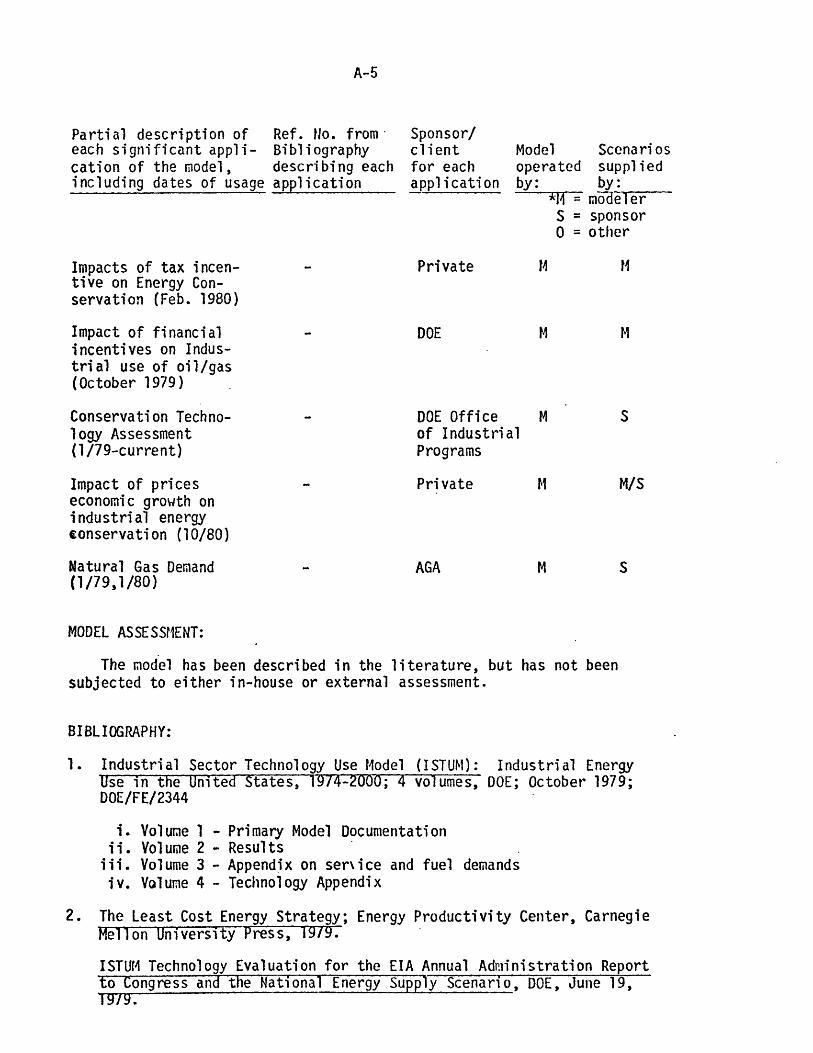
I lII IIi '

A-5

Partial description ofeach significant appli-cation of the model,including dates of usage

Ref. No. from-Bibliographydescribing eachapplication

Model Scenariosoperated suppliedby: by:

*14 = mo-delerS = sponsor0 = other

Sponsor/clientfor eachapplication

Impacts of tax incen-tive on Energy Con-servation (Feb. 1980)

Impact of financialincentives on Indus-trial use of oil/gas(October 1979)

Conservation Techno-logy Assessment(1/79-current)

Impact of priceseconomic growth onindustrial energyconservation (10/80)

Natural Gas Demand(1/79,1/80)

Private

DOE

DOE Officeof IndustrialPrograms

Private

AGA

MODEL ASSESSMENT:

The model has been described in the literature, but has not beensubjected to either in-house or external assessment.

BIBLIOGRAPHY:

I. Industrial Sector Technology Use Model (ISTUM): Industrial EnergyUse in the United States, 1974-2000; 4 volumes, DOE; October 1979;DOE/FE/2344

i. Volume 1 - Primary Model Documentationii. Volume 2 - Results

iii. Volume 3 - Appendix on ser\ice and fuel demandsiv. Volume 4 - Technology Appendix

2. The Least Cost Energy Strategy; Energy Productivity Center, CarnegieMellon University Press, 19/9.

ISTUM Technology Evaluation for the EIA Annual Administration Reportto Congress and the National Energy Supply Scenario, DOE, June 19,1iI9.

M/S

S

A- 6ENrRGY MIODEL ANALYSIS PROGRAM

r .Enerly Labor'ltor.I MasaCSC-hues tlsflulte of Tehnology

/ Camu'dcge. MAassacht

iseritS 02139

OUESTIONNAIRE FOR ENERGY POLICY MODELERS

The M.I.T. Energy Model Analysis Program (EMAP). under sponsorship from the Electric Power Research Institute. is developinga directory of energy rr.deis and assessments, to be publisned in the fall of 1980. The directory will be Oistributea w.Oely togovernment d(-.Eam nts acacemic institutions, and private industry. arC will he an extremely useful reference tool for modeldevelopers. asscssors ana u:ers We would very much like to .nclude your model in th:S directory, and therelore are requestingthat you complete the following form to provide the inlormation needed. We will then compile your responses into a standard-ized format. wnhich wil te sent to you for review prior to puoihcation.

Please answer the questions below as completely as you can: we are particularly pleased to be able to present in this directorythe kind of mear.ingful and interesting information and perspective that only mocelers and model assessors themselves canprovide. We are int rested ,n anything you have to offer about your model, and encourage you to use extra sheets of paper wherenecessary. If you are extremely sncrt of time. please answer the questions marKeC with an asterisk." Martha Mason and KellyMorgan of the EMAP will be happy to ans.er any questions and offer assistance; they may oe contacted at (617) 253-8318.

Thank you for your assistance - the directory will not be complete without an entry on your model!

GENERAL INFORMATION

*1. What is the name of the model? Industrial Sector Technology Use Model

*2. By what acronym, nickname, or other name(s) is it known? ISTU I

'3. Where, and under what auspices, was the model developed.Version I developed by ELEA under funding by ERDA/HOPPS.Version II developed by ELA under funding by DOE Conservation and Solar Divisionof Industrial Program. V-I 1977 1978

04. Over what time period was the model developed? V-_T LI0/80 to 91"moJyr moJyr.

*5. Who is the person filling out this questionnaire?

Narme: Harold Kalkstein

Address.EEA Inc., 1111 N. 19th St., Arlington, VA. 22209

Telephone 703-528-1900

Relationship tomodel Developer of ISTUI Version-Il

06. Who Is (or are) the key modeler contact(s)?

Name: Samir Salama Name* Michael Lerner

Address.EEA Inc., 1111 N. 19th St., Address. EEA Inc., 1111 N. 19th St., Arlington, VAArlington, VA 22209 Teleohone.7 03-5 2 8 -19Q0 22209

703-528-1900 Project DirectorRelationship torr ocel Proiect -Lnager Relat:onshiptomodel Project Director

*7. Who is (or are) the key contact(s) in the organization(s) that sponsored the model development?

Name. Choma;s CrossConservaton and SolarName Cyril Draffins Fossil Fnnry (Vers:in I)U nependnc Av~c., W. 100 Independence Ave., N.W

Address. . Address.

Telephone 202-252-21S20 . Telephone

Relationship to mel. Project Officer Relationship tomodel. Project Officer

MODEL CHARACTERISTICS

The following questions are designed to provide understanding of the fundamental technical characteristics of the model. Themult!plo-choice options are provided for your convenience: however, we understand that mooels vary significantly. and theseIchoices may not be suited to your model. Please add categories, phrases, or sentences, as applicable.

In Ouestion 18 ve will ask about different operating versions of the same basic model. If there has been more than one version.please indicate here which one you are describing. If the versions are significantly different. you may find it necessary to fill outa complete questionnaire for each unique model version.

*8. What keywords characterize the issues the model addresses?

[:Supply of lue!s & resources N Economic impacts of energy policies&Demand for e.ectricity O Environmental impacts of energy policiesDemand for r.cn-e,ectric energy 0 Demograpnicisocial impacts of energy policiesRegulato:y Venavior @3 New technology assessment

GElectric uttv behavor M Conservation assessmentEOtnet industry tehavlor

COther (spech)

09: What anslytic techniques are used in the model? (it appropriate, check more than one, and Indlcate which subsection ofthe model uses which technique.)CLinear programming Descriptive simulationCNontinears.nteger orogramming - Allocation & eQuilibtiumE.Othe. stat cm, .ation C InputloutputCDynamic c'rn,,: 31aon O Regression. econometric:"Stochas::c tecnniques 0 Expert oopinion. non-quantitative

COther I(spec)) _ ____ __

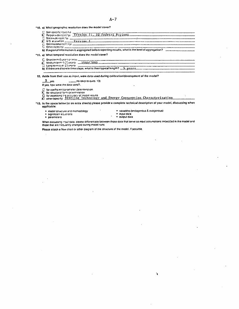
A-7

010. a) What geographic resolution does the model cover?

. Stp.soDcrtscr, ,~i , __) ___

Snternationaet T; ~ t 10 F r

C Ot rct s -ecf~,w

b) If regional informatlon is aqgregated before reporting results, what is the level of aggregation?

011. a) What temporal resolution does the model cover?

C Short terrm(5 3 '3 C' '.slX- Mediurn letrrn - years) .. 190/20L2 Long terrlmoe' 23 vyPars,b) It there are discrete time steps. what is their typical length? , 51 psn rz s

12. Aside from their use as input, were data used during calibrationldevelopmnt of the model?

X yes -- no tsk3 to queS. 13)If yes. hpw were the data usecd.

0 for coefthcen:narameter determniation3C for structural form ce:ermrnationC for assess;ng ,- arcu racit rcCel results

K otnerfspecty) Baseline Technologv and Energy Consumption Charncterizat pn

*13. In the space below (or on extra sheets) please provide a complete technical description of your model, discussing whenapplicable:

* model sruc:ure and methodology * variables (endogenous & exogenous)* significa.v e--a:or.s * input da:a* parameters * output data

When discusstng ,rnu! cata, olease differentiate between those data that serve as input assumotions imbeded in the model andthose that are fre ,ent!y changed outing model runs

Please attach a flow chart or other diagram of the structure of the model. if possible.

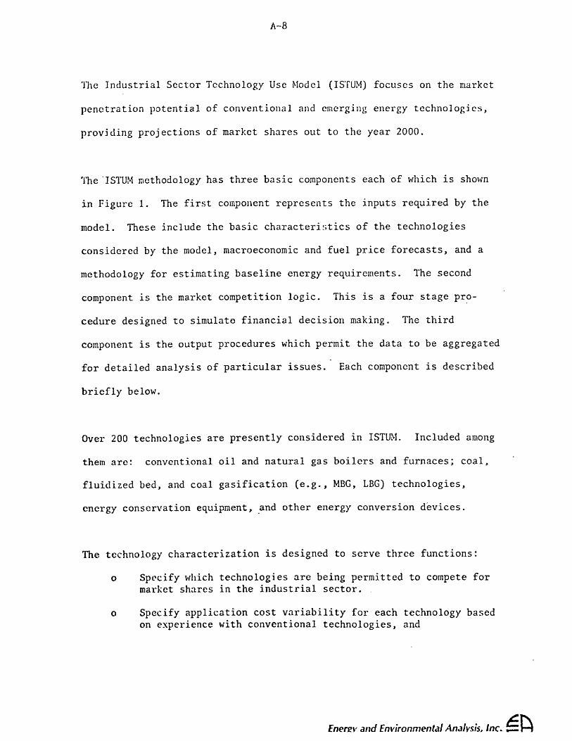
A-8

The Industrial Sector Technology Use Model (ISTUM) focuses on the market

penetration potential of conventional and emerging energy technologies,

providing projections of market shares out to the year 2000.

The ISTUM methodology has three basic components each of which is shown

in Figure 1. The first component represents the inputs required by the

model. These include the basic characteristics of the technologies

considered by the model, macroeconomic and fuel price forecasts, and a

methodology for estimating baseline energy requirements. The second

component is the market competition logic. This is a four stage pro-

cedure designed to simulate financial decision making. The third

component is the output procedures which permit the data to be aggregated

for detailed analysis of particular issues. Each component is described

briefly below.

Over 200 technologies are presently considered in ISTUM. Included among

them are: conventional oil and natural gas boilers and furnaces; coal,

fluidized bed, and coal gasification (e.g., MBG, LBG) technologies,

energy conservation equipment, and other energy conversion devices.

The technology characterization is designed to serve three functions:

o Specify which technologies are being permitted to compete formarket shares in the industrial sector.

o Specify application cost variability for each technology basedon experience with conventional technologies, and

Energy and Environmental Analysis, Inc.

A- 9

FIGURS I

SCHEMATIC OF INDUSTRIAL SECTOR TIECHNOLOGY USE MODEL

PRIM'vARY INPUTS

TEC:-u4OLCGYCHAP.ACT E IiST ICS

M +~ 7 fC-tsG. E SB ROKENt CUT .a' O' VA.;0o

*COSTS E SCLA. DO ER i*0* %AX!Mi.0A CT:CN5

DIt

I II

FUEL P.RICES.,- L E IZ D F 0, t --l: S; 3.1

%Arjr -L! t ;G- CISTRBu!CN4S TO iF -

SR!I F OR EC5sT* MACRO NCCEL*ENE4k~y M.CE!.

P l03UCTOAF~q6.CAITS

1IC US ROA L S C ,C R£NIEiuGY SVIANiO

* aY :HOuSTRYo BY SUS A:.D LOAD FACOR* ay !EACEE SEC.-OR

* BY YEAR

5VB TSC-NC LOGYI CF,l~v aums go q

sprc:,,c -.- ~.c : _____ BY '!V ' ZU-GIUCUT~t.1C1 IAI.1I1 BY .?.CU5TRY

*.3y YEAR

PRIIMARY MODEL LOGIC

FIN AM C;. L :4

C ROR A T F~A NC:A L'UC"EL

*COST OF CAPITAL* I.. -. ATCN

*ACC=L.'4'.!4G C*-NE.4TlC.1S

COST/.au 0!t.IVI!!PCR !A--4 !C'NM~tO0G

I.AWiET OCC!PETlCNANALY SI S

* 30O CCOMPETITIV5 CELLS,DC's$ E P ?A Rx1.1Y

* NI4MSRICAL SOL'JTIC84MTI-CO

Om~sINAL %I1ATCLsM.%ti~ T i9&ARIS

IACTUAL Mqt SA.

P-LJETG ,,;?I AL TURc CvE 3 M.G C EL

t NH4JS1Y IF!CaFICAaImfmT C-E'W. tS4

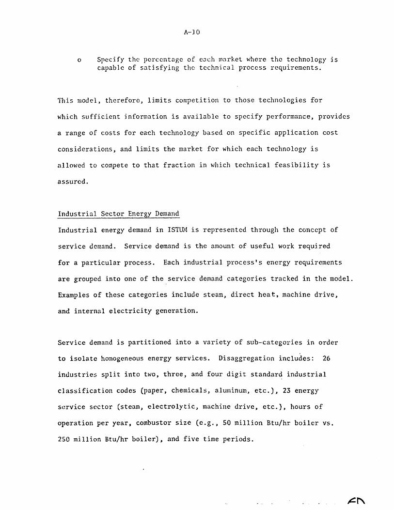
A-30

o Specify the percentage of each market where the technology is

capable of satisfying the technical process requirements.

This model, therefore, limits competition to those technologies for

which sufficient information is available to specify performance, provides

a range of costs for each technology based on specific application cost

considerations, and limits the market for which each technology is

allowed to compete to that fraction in which technical feasibility is

assured.

Industrial Sector Energy Demand

Industrial energy demand in ISTUM is represented through the concept of

service demand. Service demand is the amount of useful work required

for a particular process. Each industrial process's energy requirements

are grouped into one of the service demand categories tracked in the model.

Examples of these categories include steam, direct heat, machine drive,

and internal electricity generation.

Service demand is partitioned into a variety of sub-categories in order

to isolate homogeneous energy services. Disaggregation includes: 26

industries split into two, three, and four digit standard industrial

classification codes (paper, chemicals, aluminum, etc.), 23 energy

service sector (steam, electrolytic, machine drive, etc.), hours of

operation per year, combustor size (e.g., 50 million Btu/hr boiler vs.

250 million Btu/hr boiler), and five time periods.

Energy and Environmental Analysis, Inc.

A- 1

PRIMARY MODEL LOGIC

The fundamental assumption underlying ISTUM is that a decision to invest

in industrial equipment is based on choosing the hardware which performs

a given task at the lowest cost. However, the decision to invest is

subject to behavioral constraints which serve to restrict the market

penetration rate of emerging technologies, even though they may be

superior.

Corporate Financial Model

ISTUM considered the total cost of technology in its comparative assess-

ment, including capital costs, maintenance costs, fuel costs, and non-

fuel operating costs. Technology costs within a cell are represented as

a range rather than as point estimates and are annualized so as to

provide a basis of comparison. The distribution attempts to pick up the

effects of site specific variability, differences in equipment costs,

etc. Various tax credits, depreciation and discount rate assumptions

can be simulated in this step.

Market Competition Analysis

The determination of the initial market penetration potential is based

on the life-cycle costs calculated in the previous section. Cost dis-

tributions representing each technology competing for a market cell are

compared. The market share of each technology is determined through a

sophisticated statistical algorithm which determines the probability

that the technology is the least-cost option being considered. The

results of this step provide the economic market penetration potential.

Energy and Environmental Analysis, Inc.

_ l,

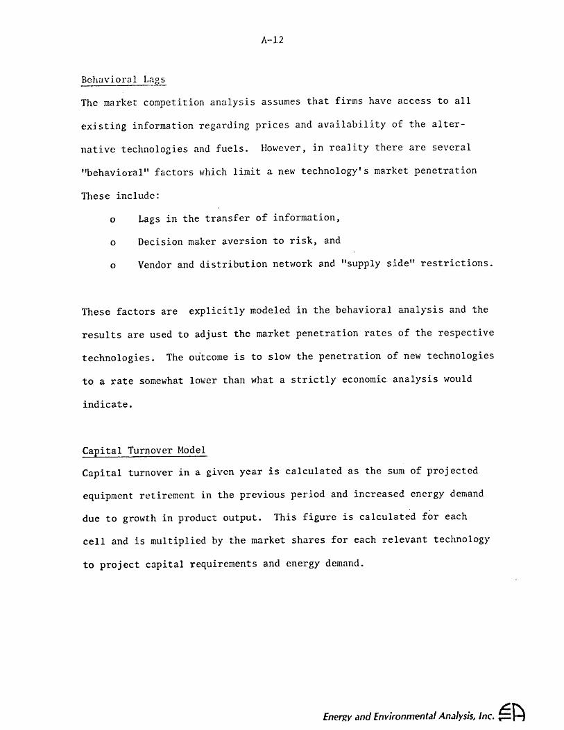
A-12

Behavioral Lags

The market competition analysis assumes that firms have access to all

existing information regarding prices and availability of the alter-

native technologies and fuels. However, in reality there are several

"behavioral" factors which limit a new technology's market penetration

These include:

o Lags in the transfer of information,

o Decision maker aversion to risk, and

o Vendor and distribution network and "supply side" restrictions.

These factors are explicitly modeled in the behavioral analysis and the

results are used to adjust the market penetration rates of the respective

technologies. The outcome is to slow the penetration of new technologies

to a rate somewhat lower than what a strictly economic analysis would

indicate.

Capital Turnover Model

Capital turnover in a given year is calculated as the sum of projected

equipment retirement in the previous period and increased energy demand

due to growth in product output. This figure is calculated for each

cell and is multiplied by the market shares for each relevant technology

to project capital requirements and energy demand.

Energy and Environmental Analysis, Inc.

A-13

Model Outputs

ISTUM provides projections of service and fuel demands at five year

intervals through 2000. Energy demands are broken down by energy service

sector, technology, fuel type, industry and technical characteristics.

Estimates of aggregate capital costs, as well as several relative measures

of market share projections are also available.

Energy and Environmental Analysis, Inc.

_1~1 I _ hu

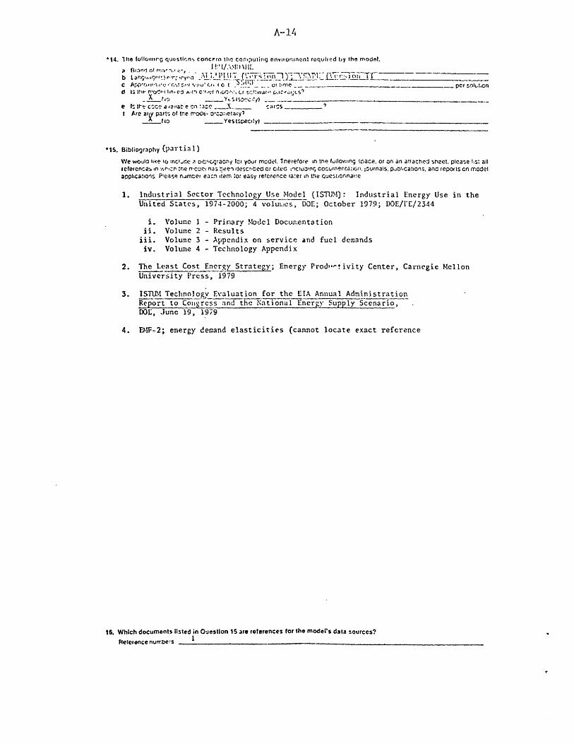
A-14

'14. Ihle lollowirg questin- concrrn the conspuing environment required by the model.

ar (3n n0f r,:-f .i .. ,_ )\ f' l ,b L ane,,')("r;cy,-... -T h . . .C Ap'ro', .: ~- 'r . )u* c' 0 .1 or t, e _ . per sol.t,cnd Is tI- n o I hIneI ,. c'.*:r nO.> .'. ,r s l wJr., .IC'L;S5

e .. It c ce as aiac e cn :ZC S. carsI Are ar part'; of tne roe, o'o:onetary'

flo Yes specly)

*15. Bibliography (partia I)

We woulo Wlie to :ncl.de i o,,c raony fcr your model. Tnerefore in the following snace. or on an attached sheet. please hst allreferences in -rtrh :ne n-cue nhas .eei 'Jescrited or cileo vncluaOn§ cocurnenlalon. journals. p.Jocanions. and reports cn modelapplhcation Please nm. er each item o: easy reference fa:er in tnte ruestionnat:e

1. Industrial Sector Technology Use Model (ISTUM): Industrial Energy Use in theUnited States, 1974-2000; 4 voluLes, DOE; October 1979; DOE/I"E/2344

i.ii.11iii.

iv.

Volume 1 - Primary Model DocumentationVolume 2 - ResultsVolume 3 - Appendix on service and fuel demandsVolume 4 - Technology Appendix

2. The Least Cost Energy Strategy; Energy Prod,,-!ivity Center, Carnegie MellonUniversity Press, 1979

3. ISTUM Technology Evaluation for the EIA Annual AdministrationReport to Co!ngress and the National Energy Supply Scenario,DOE, June 19, 1979

4. MIF-2; energy demand elasticities (cannot locate exact reference

16. Which documents listed in Ouestion 15 are references for the model's data sources?Relerence numbers -- - --

A-15

MODEL DEVELOPMENT AND APPLICATIONS

In this section Ne are intrested in tracen how tihe model has t.Le n us~t Int the first cojlumn. olease descrlbe each application ofthe mdodel. useS rra,,'t i,"Cude both ac;iJemi study and -.;-cifc rOolerm SOlvnq In tne following columns please indilcaitwhich relerence nurrtbe from OueS iirn 15 dserin.s' the aC.;iscation. who the soonsr w as for that aoplication, who actuallyoperated the n cidel. and who suggesled or supplied tIoe scurnaros rnmplemented in tri. application

Part i a Model Scenarios*Descri:ton of eac' s .;nfcant Ref. N from Sponsor/ operated suppliedapplication of !re macel. Question 15 client by: by*Includng da:es of usage describing for each M = modleer M = modeler

each applic- applic- S= sponsor S = sponsoration ation 0 other O other

Impacts of tax incentive - Private M Hon Energy Conservation(Feb. 19S0)

Impact of financial - DOE H Mincentives on Industrialuse of oil/gas(October 1979)

Conservation Technology - DOE M SAssessment (1/79 - Office ofcurrent) Industrial

Programs

Impact of prices economic - Private M M/Sgrowth on industrialenergy conservation(10/80)

Natural Gas Demand - AGA M S(1/79, 1/S0)

17. As the table above suggests. an important factor in model development and documentation Is whether or not the modelhas ever been installed and operated by someone other than the modeler.

a) Can the model be transferred for use by someone other than the modeler?X.Yes . No If no, why not'

b) Has the model ever been transferred for use by someone other than the modeler?No X Yes It ves. olease indtca'e we'e the mccel was transferred and briely Cescribe the

transferoocess Transter of ersion I to DOl: computer for planned useby Fossil Enery Di-s.ion was conpleted ai dl as su sfullrun.

c) Do you have any plans to transfer the model In the future?X No -Yes If yes. to were

18. One factor sometimes complicating model assessment Is that one-time or on-going changes to a model's structure haveled to more than one version of that model. In this question we are Interested In finding out how many discrete versions ofthe model have been developed, and which, if any, are currently operational.

a) Has the model undergone any major structural changes since Its original finished form?-No tsKp to Cues 19) ._..Yes If yes. please oriely cescr *e a-v s:;nlicant differences between the versions and

the reasons molivatin; tre cnarges.

i )Which version(s) of the model are currently operational, and where are they maintained?

Version 1; .Maintained on STSC computer system-is operational.

Version 2: Maintained on EIA/DOE computerywill be operational in the fall.

1hi

A-16

MODLL ASSESSM[NT

*19. Haes the model ever been ,ubjocled to an in house assousniont by the modtrlors?

.Not,.'0 otiO:'; 20C) (not rfornl. ly)

Yes a) If yes. which clmonlts listed below received empha is during the niodelor assessment?L Mod, vtdty ' " Usabillity

C; Structure Documentation

C Content 0 Efficiency0 Preociton C Model

C Data val-ddy applicationsSVerification of the C Other (specify)

model's expressionin the computercode

b) Please briefly describe the techniques utilized irs the modeler assessment.

*20. Has the model been made available for assessment by external parties?

G No (skip to OJeston 21)f6 Yes. thCroUn cucitcation of model descrotions in the literature.C Yes. throun a formal external assessment£I Yes. thro~,gh other meansispecify)

If the nooet v.as assessed by an Individual. group or organization other than the modeler(s). please answer the questions below.

a) Who was the assessor for the model?

Organization Technokron

Name of contactTitle

Address -

Telephone ( )Title of Report

b) Who sponsored the assessment?

Organization Fossil Energy Division, DOE

Name of conact C'ril[ Irat inTitle -Address - _3' I MgA _'n F 8 .L Z O

Telephone (

c) What assessment approach(es) were employed by the assessors?

Ot Review of the f;terature. not inclujng the computer code

0 Evaluation of the detaiied dccurentation. incudind the codeC Audit of the mccel's performance, using test problems0 Evaluation of the model using experiments cesigned by the assessors. but imolemented by the modelers

o In-depth assessment. in wiich the assessors themselves implemented experimental runs of the model

G Comparative evaluation of two or more models0 Other (specify)

d) Which elements listed below received emphasis during the external assessment of the model?

El Model validity 0 Usability:l Structure 0 DocumentationO Content 0 Elficiencyo Prediction 0 Model

O Data validity applicationso Verification of the 0 Other (specify)

model's expressionIn the computercode

e) Do you have any comments on the external evaluation of the model?

21. a) Please discuss the accessibility of the model for initial or further as .essment. If the model has not been assessed. do

you have any plans concerning future assessment? Do you feel it r hould be considered for an assessment?

Version II of the Model will be in the public domain, fully doctumented and

_Xlilblcto._mrc -Q%," by t "b liTDO 3L N2__._o exten,;Lye external rcview.js p rvetmt, 0., ,1 otjV m T .Ll t) F-u J'- - 5 S-Tdi-R'

expert , - part ot a vali d,1Ft.ask in tte projiect.

22. We would be interested In any other aspects of the model that you would like to discuss. How doesit compare with other

models in terms of structure or coverage? Were there any interesting ramifications resulting from use of the model?

A-17

Additional Information and Comments on ISTUM

ISTUM computes energy demand and technological market shares from

technological costs and efficiencies, service sector demand, and fuel

prices.

Fuel prices are built into ISTUM, but can also be input by the user.

Fuel prices are entered as distributions as opposed to point estimates in

ISTUM. Thus they are characterized by their mean, variance, and minimum

values. This is done to capture regional differences in prices. The

ISTUM fuel prices were provided by Data Resources, Inc. from the DRI U.S.

Annual Energy Model. Fuel prices are input adjusted to the specific

technology with which the fuel is used. This is done by dividing the

fuel price by the conversion efficiency of the technology. This is done

so that all fuel prices reflect the cost of the energy produced that is

usable to industry in a constant manner.

In order to determine total energy demand, ISTUM must first determine

the demand for each of the 23 service sectors. To do this ISTUM divides

industrial demand into 26 Standard Industrical Classifications (SICs).

Each of these SICs has a certain demand for each service sector. These

demands are then aggregated to determine total service sector demand. To

project future service demand ISTUM assumes that service demand grows at

the same rate at which the industry does. These projections were also

made by DRI on their Quarterly Macroeconomic Model. Since there are

differences in ISTUM4's and DRI's industrial classifications, surrogates

for service sectors are used in some projections.

ISTUM divides industrial use of energy into 23 service sectors. Of

these, thirteen actually compete technologies to fill the demand. The

other ten are sectors such as feedstocks that are included in the model

I-----~ Yli i

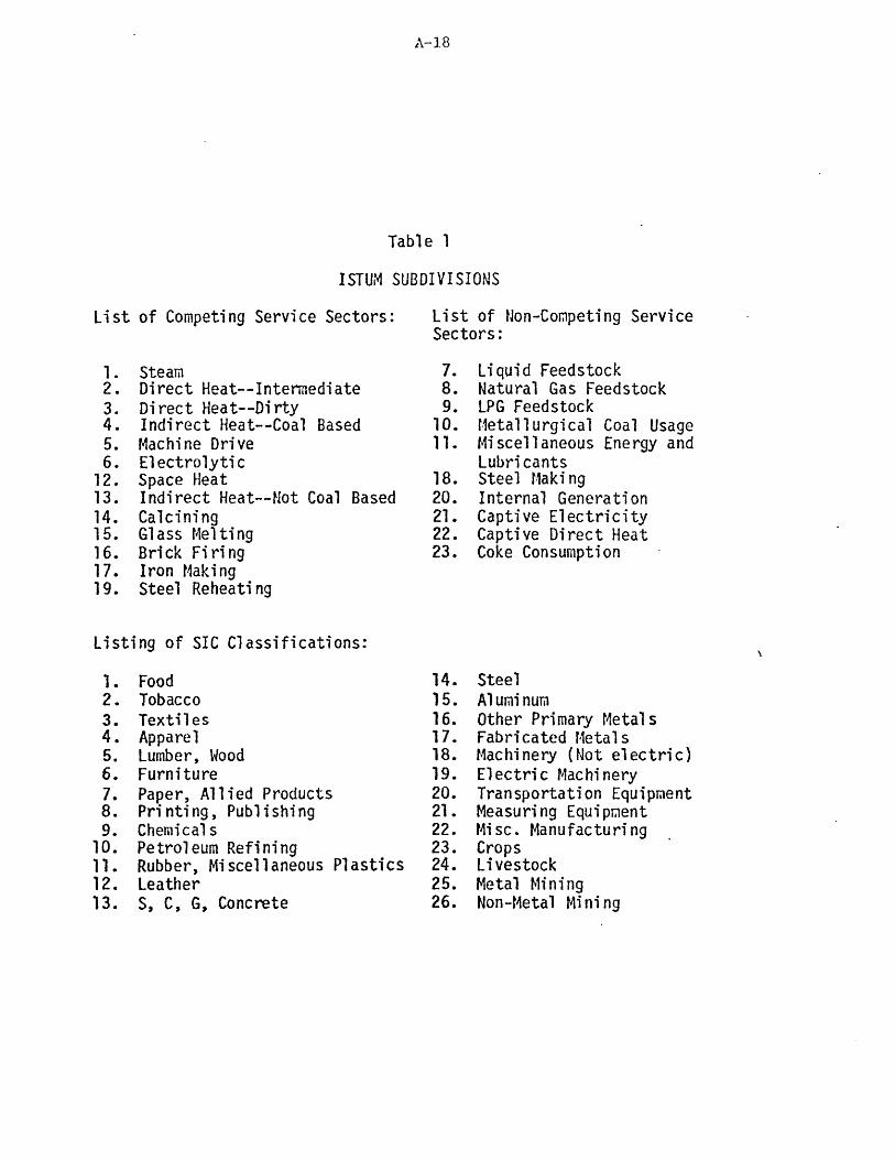
A-1.8

Table 1

ISTUM SUBDIVISIONS

List of Competing Service Sectors:

1. Steam2. Direct Heat--Intermediate3. Direct Heat--Dirty4. Indirect Heat--Coal Based5. Machine Drive6. Electrolytic

12. Space Heat13. Indirect Heat--Not Coal Based14. Calcining15. Glass Melting16. Brick Firing17. Iron Making19. Steel Reheating

Listing of SIC Classifications:

S1.2.3.4.5.6.7.8.9.

10.11.12.13.

FoodTobaccoTextilesApparelLumber, WoodFurniturePaper, Allied ProductsPrinting, PublishingChemicalsPetroleum RefiningRubber, Miscellaneous PlasticsLeatherS, C, G, Concrete

List of Non-Competing ServiceSectors:

7.8.9.

10.11.

18.20.21.22.23.

14.15.16.17.18.19.20.21.22.23.24.25.26.

Liquid FeedstockNatural Gas FeedstockLPG FeedstockMetallurgical Coal UsageMiscellaneous Energy andLubricantsSteel MakingInternal GenerationCaptive ElectricityCaptive Direct HeatCoke Consumption

SteelAluminumOther Primary MetalsFabricated MetalsMachinery (Not electric)Electric MachineryTransportation EquipmentMeasuring EquipmentMisc. ManufacturingCropsLivestockMetal MiningNon-Metal Mining

-- Ifi.

A-19

to insure that total industrial energy usage is accounted.

A problem with this service sector approach is that the service

"' provided by an individual service sector is not totally homogeneous. One

solution to this problem is to increase the number of service sectors.

ISTUM service sectors calcining, glass melting, brick firing,

iron-making, steel-making, and steel reheating are separated from the

direct heating sectors because of such problems.

A similar type of problem was solved by using size and load factors

in the ISTUM service sectors. It is reasonable that technologies will be

more or less competitive depending upon their size or load factor. Size

refers to the MI4Btu's produced per hour and load factor to the number of

hours per year a technology is in use. Part of this size and load effect

is captured by the use of cost distributions. However, for more accurate

• predictions up to two size and two load factors for each service sector

are used. More precision might have been available by using more sizes

and load factors, but at a trade-off in model costs.

Technologies are the third important input in determining final

energy demand. Good descriptions of the engineering processes of the

technologies can be found in the ISTUM documentation.

Like fuel prices, technologies are represented by cost

distributions. The use of a distribution more accurately portrays costs

than single point estimates. Costs vary for a number of reasons.

Construction costs vary according to site specifications and labor

costs. Also the quality of the service (e.g., evenness of heat) needed

by different industries may vary costs. To calculate capital costs, the

costs are broken down into components, estimated, and then aggregated.

The components are:

A-20

1) site preparation and power house

2) primary systems and controls

3) fuel handling

4) environmental controls and waste handling

5) utility and feedwater systems

6) indirect capital costs

7) installation costs.

When technology costs are finally input into ISTUM they are given in

$/MMBtu's and annualized. The capital charge rate not only takes capital

lifetime and rates of return into consideration, but also the effects of

tax laws and depreciation accounting procedures.

Originally ISTUM was to look at different costs depending upon

whether a new or old plant was implementing the technology. The

empirical data suggest that a great difference in costs does not exist,

so the distinction was not included in the model.

Technologies are given a maximum market penetration. This figures

may be 100% of the service sector. Maximum shares exist for many

reasons. A technology may not provide the correct quality of service

across the whole sector. Steam is an example. Solar technologies cannot

provide the higher-pressure steam needed by solme industries. Thus it has

a maximum market share. Environmental constraints may also limit a

technology's market share.

ISTL 4 only competes technologies to fill incremental service demand.

This is demand created by increases in service demand plus demand created

by retirement of capital. The retirement schedule is based upon

historical trends. In general, the older the capital, the higher its

retirement rate. ISTUM does not allow for early retirement of uneconomic

A-21

capital.

In competing technologies to fill the service demand, it is important

to remember that costs are represented by distributions. By taking

annualized capital and operating costs and adding them to fuel costs,

ISTUM produces a total cost distribution. Since distributions tend to

overlap, a combination of technologies will capture shares of the

market. The minimum total cost value is important here. Otherwise all

technologies would capture a non-zero market share.

The market shares thus obtained are then modified by the behavioral

lag component. This component reduces the introduction of new

technologies. The newer a technology, the greater the lag will be.

After accounting for this behavioral lag, the market shares are

recalculated. These shares are turned into actual capital investment by

multiplying by the incremental energy demand. Total fuel use is then

calculated from the technologies in use.

~~11"i".

. ... .. , ,,,,,, , 1= I 1mim

A-22

3. Transportation Energy Conservation Model (TEC)

Energy Model Analysis Notebook Entry

MODEL NAME:

ANALYTIC TECHNIQUES:

ISSUES ADDRESSED:

DEVELOPED:

RESOLUTION:

ASSESSMENT:

MODELER CONTACT:

SPONSOR:

Transportation Energy Conservation Model TEC

Linear ProgrammingRegression, econometric

Demand for Non-Electric EnergyRegulatory BehaviorOther Industry BehaviorNew Technology AssessmentConservation Assessment

o 1976-1978

Geographic: U.S. as a wholeTemporal: long term 1975-2025;

single year up to 2000;five year steps to 2025

Partial - Automobile sector forecasting model -independent assessment by University of MichiganHighway Safety Research Institute

Mike LaurenceJack Faucett Associates5454 Wisconsin Ave.Chevy Chase, MD 20015301 -657-8223

Gary KaitzStanford Law SchoolPalo Alto, CA 94305

Department of Energy - Applied Analysis

MODEL DESCRIPTION:

TEC is designed to compute energy usage in the transportation sectorbetween the years 1975 and 2025. The model is divided into ninetransporation modes - air, automobile, truck, bus, motorcycle, rail,marine, and pipeline. The modes are independent and can be run togetheror in any combination of the nine. TEC is a demand for transporationservices model in which the manufacturers minimize the lifetime vehiclecosts to the consumer. The model can consider factors such as fuelprices, vehicle miles demanded, cost of improved efficiency,environmental and safety factors, tax effects, and the introduction ofnew technologies.

The automobile mode is the most complex of the nine modes. The modelclassifies autos into three weight classes and projects a demand for each

- IENEI GY MODEL ANALYSIS PROGRAM

S Enerfi, Labonrao'ry. Mas<chu elts Ins:'ue of Technology

. Cambrnajg., .Lassachcse::s 02139

QUESTIONNAIRE FOR ENERGY POLICY MODELERS

The M.I.T. Energy Model Analysis Program (EMAP). under sponsorship from the Electric Power Research Institute. is developinga directory of energy models and assessments. to be published in the fail of 1950. The directory will be distributed widely togovernment departments. academic institutions, and private Industry. and w:il be an extremely useful reference tool for modtldevelopers. assessors, and users. We would very much like to include your model in this directory, and therefore are re-uestingthat you complete the following form to provide the information needed. Vie will then compile your responses into a standard-ized format, which will be sent to you for review prior to publication.

Please answer the questions below as completely as you can: we are particularly pleased to be able to present in this directorythe kind of meaningful and interesting informat:on and perspective that only modelers and model assessors themselves canprovide. We are interested in anything you have to of fer about your model. and encourage you to use extra sheets of paper wherenecessary. If you are ex!rernmely short of time. please answer the questiors rmared t' an astenrsk.' t.artha Mason and Ke;lyMorgan of the EMAP wili be happy to answer any questions and offer assistance: they may be contacted at (617) 253-8318.

Thank you for your assistance - the directory will not be complete without an entry on your modell

GENERAL INFORMATION

*1. What is the name of the model?

2. ransortation Energo y ConsratiJ~n Model*2. By what ac/onym, nickname. or eoffel namets) Is it now

TEC*3. Where, and under what auspices, was the model developed.

Developed by Jack Faucett, Associates under funding from ERDAConservation and Solar Applications, Office of Transportation Programs

*4. Over what time period was the model developed? --- 6-- tomo yr. moyr.

*5. Who Is the person filling out this questionnaire?

Name, Michael F. I awrnce-Address -- 4- ire 4- i .. , C 2hevy' lh Mn 2001Telephone. 301-657-8223

Relationship to model.

'6. Who is (or are) the key modeler contact(s)?

Name: Michael F. LawreLce Name...Gary Kait7

Address, AddressStanford Law School. Palo Alto,_CA

Telephone: Telephone: 94305

Relationship to model:c Relationship to model: pro rammer

*7. Who is (or are) the key contact(s) in the organization(s) that sponsored the model development?

Name: ._ em.y -raboyL Name

Address: DOE- Aplied Analysis.-, ashbi nrt-on,_ C . ?n467

Telephone: 2-0 . j63 --.& -S Telephone:

Relationship to model:.Pt e ct Z r iS..t._.... Relationship to model:

MODEL CHARACTERISTICS

The following questions are designed to provide understanding of the fundamental technical characteristics of the model. Themultiple-choice options are provided for your convenience; however, we understand that models vary significantly, and thesechoices may not be suited to your model. Please add categories, phrases, or sentences, as applicable.

In Question 18 we will ask about different operating versions of the same basic model. Itf there has been more than one version.please Indicate here which one you are describing. If the versions are significantly different, you may find it necessary to till outa complete questionnaire for each unique model version.

08. What keywords characterize the Issues the model addresses?

OSupply of fuels & resources 0 Economic impacts of energy policiesM)Demand for electricity 0 Environmental impacts of energy policies

!p0emand for non-electric energy 0 Demographic/social impacts of energy pa;oicesaR-'gulatory behavior I New technology assessment

UlElectric utility behavior fr Conservation assessment(jOther industry behavior

l Other(specify)

*9. What analytic techniques are used In the model? (If appropriate, check more than one, and Indicate which subsection ofthe model uses which technique.)

(XLinear programming O Descrnipive simulAtionONonlinearinteger programming 0 Allocation & equilbrlumOOther stalic optimi:allon U Input/outputCODynamic optmlzation IR Regression. econometricOStochastic techniques U. Expcrt opinion, non-quantitative

Other (specify) _ ___ __ ____

A-22b*-10. a) What geographic resolution does the model cover?

[1 Site-spectifc (spec1y)"U. Regtonwide (pectly)i ] Statewlde tspecly)CX U S asa whole-L; International (specify)L; Oher (specify)b) If regional information is aggregated before reporting results, what is the level of aggregation?

*11. a) What temporal resolution does the model cover?

U Short term (S years or less)t. Medium lerm(6-20 years)L k Long term(over 20vyears --- 97-502 5-_b) If there are discrete time steps, what is their typical length? SA T ear TtPUO ZO O7

fivp year steps uptoZ 2512. Aside from their use as input, were data used during calibrationldevelopment of the model?

..X yes no (skip to ques. 13)If yes. how were the da!a used)

•Zj- for coeff,cient!parame:e; de:eainaionC for structural form dee:mina:.onCk for assessing the accuracy.ol model results[ other (specify)

*13. In the space below (or on extra sheets) please provide a complete technical description of your model, discussing whenapplicable:

* model structure and methodology * variables (endogenous & exogenous)* significant equations * input data* parameters * output data

When discussing input data. please differentiate between those data that serve as input assumptions imbedded in the model andthose that are frequently cnanged during model runs.

Please attach a flow chart or other diagram of the structure of the model, if possible.

see attached

A-22c

MODEL DESCRIPTION

TEC is designed to compute energy usage in the trans-

portation sector between the years 1975 and 2025. The model

is divided into nine transportation modes - air, automobile,

truck, bus, motorcycle, rail, marine and pipeline. The modes

are independent and can be run together or in any combination

of the nine. TEC is a demand for transportaion services model

in which the manufacturers minimize the lifetime vehicle costs

to the consumer. The model can consider factors such as fuel

prices, vehicle miles demanded, costs of improved efficiency,

environmental and safety factors, tax effects, and the intro-

duction of new technologies.

The automobile mode is the most complex of the nine modes.

The model classifies autos into three weight classes and projects

a demand for each weight class. It then determines the demand

for new cars by calculating the scrapage rate of the existing

fleet and by finding the difference between fleet demand and

number of cars in the fleet minus scrappage. The model then

fills the new car demand with the cars that minimize the total

of the initial costs and the discounted operating costs over

the first owner's lifetime of the car. The car life for the

first owner is assumed to be approximately 52,000 miles.

Future costs are discounted at 10% for 80% of the car buyers.

The other 20% are assumed not to consider operating costs when

making their purchase. The costs of increased fuel efficiency

are built into the model and the fuel prices may be changed for

A-22d

all years of the run. The costs of the technologies to improve

fuel efficiency are considered seperately for three time blocks

within the model. The model also includes different safety and

emitions scenarios and can check the effect of MPG requirements

and penalties for non-compliance.

The truck and air modes are similar in design to the auto

mode. Trucks are divided into light, medium, heavy and heavy-

heavy weight classes. Airplanes are divided into six categories

for commercial flight and one general aviation class.

The other modes are simpler in design than the first three.

This is due largely to data constraints.

TEC offers output on fuel consumption and costs, vehicle

costs and vehicle market shares.

14. 1he followinu cquvs.lion coancern the conilmuling envronmmcn! reqluierd by Iie InoIVr.

a. Brindo ,,, ,y . I , o y A-2 2eb. Lang age(-) om, oyed . I Fi,' . .. ....C. Approvin.te coAp "r solutiOn co t _.. or li rne pe .llilutes . .. per so utord. IS the model hn; .idl with other rnc=cels or software package

_X_ .4lo __Yes(specify)e. Is the code available on ta. _yyes5 cards ..yes ?I. Ar& any parts of the rmodel proprietary?

_ _.No -- Yes(specify)

*15. Bibliography

We would like to include a bibtiog-aphy for your model lherefore. in The fo:owtng soace. or on an attached sheet. please list a:.references in which the model has been described or cited: Including oocunmen:a:,on. journa!s publications. and reoorts On moC'applications Please number each item for easy reference later in tne q'Jestionnare

1. Jack Faucett Associates, TEC: Transportation Energy Conservation Model,Washington, D.C. JFA, 1978

2. Jack Faucett Associates, TEC: Transportation Enerqy Conservation Model-Uer's GuideWashington, D.C., JFA, 1978

3. The Energy Productivity Center, Least-Cost Energy Strategy-Technical Appendix ,Carnegie-Mellon University Press

4. Shackson, Richard H. and Leach, IH. James, Maintaining Automotive MobilityLUsing Fuel Economy and Synthetic Fuels to Compete with OPEC Oil, Interim Ieport,Carinegie-Mellon University Press, 1980

5. Jack Faucett Associates, Automobile Sector Forecasting Model Documentation,Washington, D.C. OFA, 1978

16. Which documents listed In Question 15 are references for the model's data sources?

Reference numbers:

A-22fMODEL DEVELOPMENT AND APPLICATIONS

Ir this section we are interested in tracing how the model has been used In the first column. please describe each application ofthe model. uses might include both academic study and specific problem-solving. In the following columns please nadscatewhich reference number from Question 15 describes the application, who the sponsor was for that application, who actuallyoperated the model, and who suggested or supplied the scenarios implemented in the application.

*Description of each signifcantapplication of the model.including dales of usage

Least-Cost Energy StrategyStudy

Ref. # fromQuestion 15describing

each applic.ation

Model SenarioScenariossupplied

by:M = modelerS = sponsorO = o:ner

S3,4

Sponsor/client*

for eachapplic-ation

MellonInstituteEPC

I I 1

17. As the table above suggests, an important factor In model development and documentation is whether or not the modelhas ever been installed and operated by someone other than the modeler.

a) Can the model be transferred for use by someone other than the modeler?x Yes No If no. why not?

b) Has the model ever been transferred for use by someone other than the modeler?No _.XYes II yes. please indicate where the model was transferred and briefly descrnte. the

transfer process. mOl was tr.Sa~ne9ie.-etton-Uni-ver- f t

c) Do you have any plans to transfer the model in the future?.X No Yes II yes. towhere?

18. One factor sometimes complicating model assessment is that one-time or on-going changes to.a model's structure haveled to more than one version of that model. In this question we are Interested in finding out how many discrete versions ofthe model have been developed, and which, if any, are currently operational.

a) Has the model undergone any major structural changes since Its original finished form?.. No (skip to ues. 19) Yes It yes, please briefly describe any signl'cant differences between the versions and

the reasons motivating the changes.

b )Which version(s) of the model are currently operational, and where are they marlntained?

-- I -- -Model

operatedby:

M= modelerS= sponsor

O = other

MODL 3 ESSMENT

'19. Has the model ever been subjected to an in-house assessment by the modelers?

No (skip to Oue; 20)

_JLYes a) If yes, which elements listed below received emphasis during the modeler assessment?LX Model validity L. Usability

,; Struclure [3 DocumentationJO Content Efficiency

k' Prediction C ModelData va!:iaty applications

. Verification of the 0 Other (specify)model's expressionin the computercode

b) Please briefly describe the techniques utilized in the modeler assessment.

*20. Has the model been made available for assessment by external parties?

0 No (skip to Ouestion 21)0 Yes. through pubhcat:oa of model descriptons in the literature.y" Yes. through a formal ex:-'nal assessment assessment done of Automobile sector0 Yes, through ot.er means(specify)

If the model was assessed by an individual, group or organization other than the modeler(s), please answer the questions below:

a) Who was the assessor for the model?

Organization Uniersty of _ichiganrdighwa h S f.ety Research InstituteName of contac LBarba ra-URicardso nTitleAddress .fDniar&'rity _K c.igajl -HSrRT

2~_201Baxter Poadr

Telephone(131}) 753-1 7&-itle ol Repordl__tP _pulished fa!.__Q78

b) Who sponsored the assessment?

Organization otL0 ._V.ehi lanufactu sName of conlactDl Vk Sh ckS tonTitleAddress

Telephone( )

c) What assessment approach(es) were employed by the assessors?

0 Review of the literature, not including the computer coderi Evaluation of the detailed documentation, including the code10 Audit of the model's performance. using test problemso Evaluation of the model using experiments designed by the assessors. but implemented by the modelers

J0 In-depth assessment. In which the assessors themselves implemented experimental runs of the model0 Comparative evaluation of two or more modelso Other (specify)

d) Which elements listed below received emphasis during the external assessment of the model?

RI Model validity 0 UsabilityxJ Structure 0 DocumentationXJ Content 0 Efficiency91 Prediction 0 Model

kl Data validity applicationsgi Verification of the 0 Other (specify)

models expressionIn the computercode

e) Do you have any comments on the external evaluation of the model?

21. a) Please discuss the accessibility of the model for initial or further assessment. If the model has not been assessed, doyou have any plans concerning future assessment? Do you feel it should be considered for an assessment?

22. We would be Interested in any other aspects of the model that you would like to discuss. How does It compare with othermodels in terms of structure or coverage? Were there any interesting ramifications resulting from use of the model?

A-23

weight class. It then determines the demand for new cars by calculatingthe scrappage rate of the existing fleet and by finding the differencebetween fleet demand and number of cars in the existing fleet minusscrapage. The model then fills the new car demand with cars that

*" minimize the total of the initial costs and the discounted operatingcosts over the first owner's lifetime of the car. The car is assumed tolast 52,000 miles. Future costs are discounted at 10% for 80% of the carbuyers. The other 20% are assumed not to consider operating costs whenmaking their purchase. The costs of increased fuel efficiency are builtinto the model and the fuel prices may be changed for all years of therun. The costs of. the technologies to improve fuel efficiency areconsidered separately for three time blocks within the model. The modelalso includes different safety and emissions scenarios and can check theeffect of MPG requirements and penalties for non-compliance.

The truck and air modes are similar in design to the auto mode.Trucks are divided into light, medium, heavy and heavy-heavy weightclasses. Airplanes are divided into six categories for commercial flightand one general aviation class.

The other modes are simpler in design than the first three. This isdue largely to data constraints.

TEC offers output on fuel consumption and costs, vehicle costs andvehicle market share.

COMPUTING ENVIRONMENT:

o Machinery: IBM 370

o Language: FORTRAN

o Approximate time per solution: 2 1/2 minutes

o Model is non-proprietary

o Model can and has been transferred

o Model is available on tapes and cards

MODEL DEVELOPMENT AND APPLICATIONS:

The TEC model was developed around the Jack Faucett Associates'Automobile Sector Forecasting Model. The Automobile Sector Forecastingmodel is now a fully integrated part of the TEC model; however, like allthe sectors of TEC, it may be run separately.

The only current application of the TEC model is its use in theMellon Institute's Least-Cost Energy Study.

------ -6 l,,

A-24

Description of eachsignificant applicationof the model, includingdates of usage:

Ref. No. fromBibliographydescribing eachapplication

Sponsor/client Model Scenarios.for each operated suppliedapplication by: by:

*M = modelerS = sponsor0 = other

Least-Cost EnergyStrategy Study

3,4 MellonInstituteEPC

MODEL ASSESSMENT:

Assessor:

Sponsor:

Barbara RichardsonUniversity of Michigan Highway Safety Research Inst.2901 Baxter RoadAnn Arbor, Michigan 48109313-763-1276

Motor Vehicle Manufacturers Association

An in-house assessment of the TEC model was performed. The validityof the model's structure and content were checked. Tests were also runto check the model's predictions. The in-house assessment also verifiedthe computer code.

An in-depth external assessment of the Automobile Forecasting Sectorof the TEC model was performed by the University of Michigan HighwaySafety Research Institute. This work included recalculation of the datainputs and the parameters of equations used in the model. Test data wererun to check the accuracy of the model's forecasts. This assessment alsoexamined the model's computer code.

No other assessments are planned at this time.

BIBLIOGRAPHY:

1. Jack Faucett Associates, TEC: Transportation Energy ConservationModel, Washington, D.C., JFA, 19/8.

2. Jack Faucett Associates, TEC: Transportation Energy Conservation -User's Guide, Washington, D.C., JFA, 19/8.

3. The Energy Productivity Center, Least-Cost Energy Strategy -Technical Appendix, Carnegie-MelFon---Fiversity Press.

m~

A-25

4. Shackson, Richard Hi. and Leach, H. James, Maintaining AutomotiveMobility: Using Fuel Economy and Synthetic Fuels to Compete with OPECOil, Interi Ti Report, Carnegle-Mellon University lress, 1980.

5. Jack Faucett Associates, Automobile Sector Forecasting ModelDocumentation, Washington, D.C., JFA, 19/8.

--

A-26

Additional Information and Comments on TEC

The TEC model used in the Least-Cost Strategy Study is on the

Carnegie-Mellon University computer. Thus it is possible that changes

were made to the model which may make it different than the description

below. Recently, an evaluation of the Automobile Sector Forecast Model

(the automobile sector of TEC) was performed by the University of

Michigan Highway Safety Research Institute. This report should be

available in the fall. The report did suggest changes that must be made

in the model to insure reliability of the results. When this report

becomes available, it should provide valuable insights into the rest of

the TEC model and the Least-Cost Study. The Least-Cost Study only

appears to use the aircraft, automobile, and truck sectors of TEC. Thus

they will be the only ones discussed here.

The aircraft sector is divided into two parts: air carrier and

general aviation. The Least-Cost Study does not appear to consider

general aviation in its analysis. The air carrier sector is further

divided into two components, domestic and international travel. This is

because the two types of travel have somewhat different characteristics.

However, the methodology involved in calculating fuel use is the same.

TEC divides aircraft into six categories according to number of

engines and body type (i.e., narrow or wide). Current aircraft are

placed into these groups. Fuel efficiency gains are made by replacing

existing planes with more efficient planes. The more efficient planes

are phased in according to a schedule based on various studies. TEC

contains two alternative schedules which may be used. One is based upon

the assumption that research being done by NASA will become available.

This schedule is considerably more optimistic about fuel efficiency

A-27

increases than the other schedule that does not assume the NASA research

will be available.

The aircraft sector first projects total passenger-miles for a given

year. These estimates are based upon an FAA study. However,

passenger-miles can be input by the model user. Passenger-miles are then

converted to seat-miles by dividing by load factor. TEC assumes a

constant load factor of .55. This figure can also be changed by the user.

Seat-miles are then allocated into each of the different aircraft

groups. The percentages to each category are held constant by the

model. Within each category seat-miles are then allocated to specific

aircraft. To do this a retirement schedule based upon assumed aircraft

lifetime is applied to the fleet to determine size of existing fleet.

Seat-miles are first distributed among the existing fleet. Remaining

seat-miles are then allocated to new planes. It is assumed that the most

fuel-efficient planes available will be purchased. From this information

fuel consumption can then be determined.

The automobile sector begins by projecting a demand for automobiles

in a given year. This is done as a function of household income.

Different household income levels are assumed to have different demand

levels. The parameters were developed from historical data. Total

automobile fleet demand is figured by aggregating the number of

automobiles demanded by each income level. The demand for new cars is

then determined by subtracting current fleet size from the total

automobile demand plus scrappage. The scrappage schedule is based upon

historical trends. The effect of new car prices and the unemployment

rate on scrappage is also added for automobiles nine years or older.

The new car demand is filled by cars that minimize the total

.11

A-28

discounted costs to the first owner, or about 52,000 miles. The data on

costs of increasing fuel efficiency were taken from a Hittman Associates,

Inc. study. The study looks at different technologies and estimates

their cost and fuel savings. Future costs are discounted at 10% for 80%

of car buyers. The other 20% are assumed not to consider future costs in

their purchase decision.

TEC divides the automobile market into three groups depending upon

weight. Market shares of each of the three weight classes are based upon

historical data and are a function of the relative prices of cars of

different weight classes and the market share of the weight class in the

previous time period.

TEC also computes vehicle miles traveled per year per household.

This is a function of disposable income, number of automobiles owned, and

the real price of fuel. From the information on weight class, fuel

economy of cars, and vehicle miles traveled, TEC calculates fuel

consumption. In this calculation an adjustment is made to simulate the

fact that as a vehicle gets older it is used less often.

The light truck sector is modeled in a similar way except no

competition exists among fuel-saving technologies. Yearly fuel economics

are simply put into the model.

The trucking sector is also similar to the automobile sector. The

trucks are divided into three types: medium, heavy, and heavy-heavy.

The trucks are also divided into seven categories according to their use

(e.g., construction, agriculture). Demand for truck use in each of these

categories is predicted. This demand is a function of growth in GNP.

New truck demand is figured from demand, existing fleet, and scrappage.

Vehicle miles traveled are then calculated and fuel efficiency can be

A-29

calculated. The fuel efficiencies of different model years are taken

from earlier research by Jack Faucett Associates. From information about

vehicle miles traveled, fuel efficiencies and the age mixture of the

truck, fleet fuel consumption is calculated.

- -~-~---61 11iili

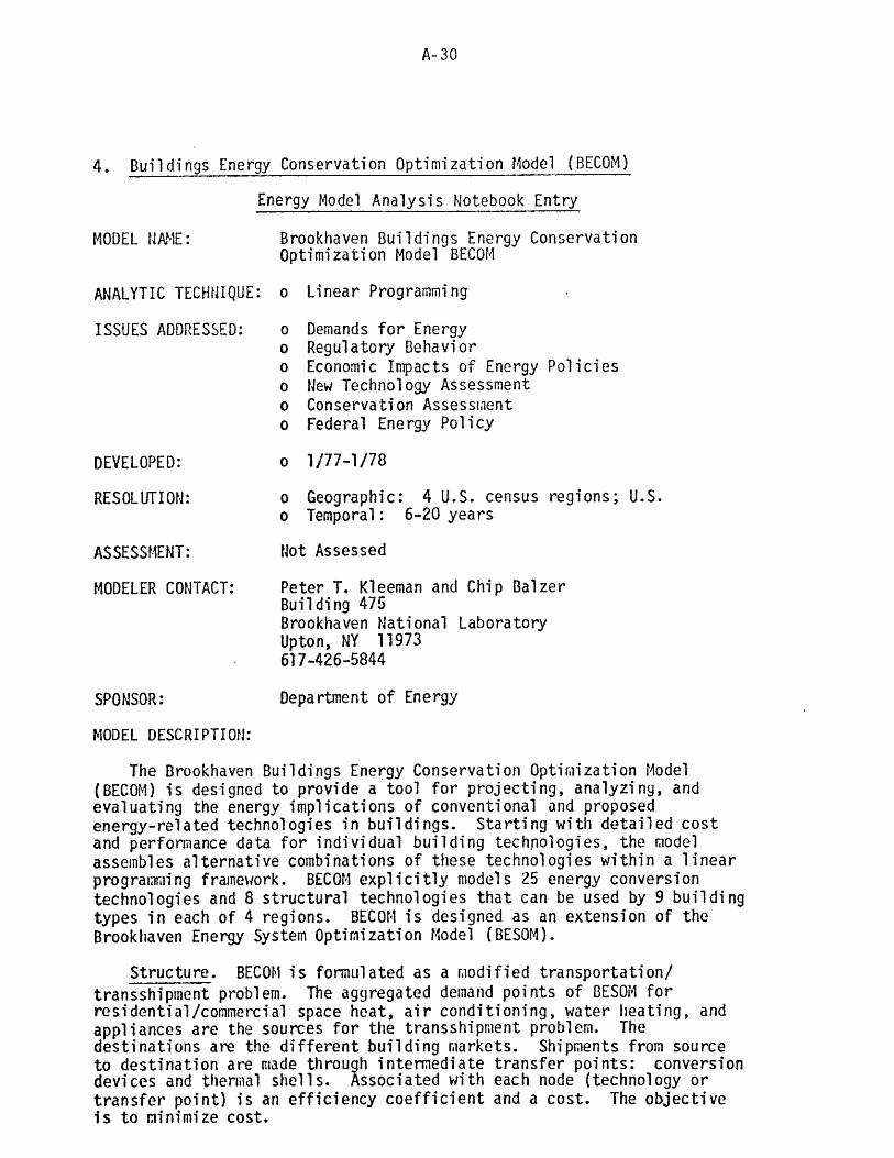
A-30

4. Buildings Energy Conservation Optimization Model (BECOM)

Energy Model Analysis Notebook Entry

MODEL NAME:

ANALYTIC TECHNIQUE:

ISSUES ADDRESSED:

DEVELOPED:

RESOLUTION:

ASSESSMENT:

MODELER CONTACT:

SPONSOR:

Brookhaven Buildings Energy ConservationOptimization Model BECOM

o Linear Programming

Demands for EnergyRegulatory BehaviorEconomic Impacts of Energy PoliciesNew Technology AssessmentConservation AssessmentFederal Energy Policy

o 1/77-1/78

o Geographic: 4 U.S. census regions; U.S.o Temporal: 6-20 years

Not Assessed

Peter T. Kleeman and Chip BalzerBuilding 475Brookhaven National LaboratoryUpton, NY 11973617-426-5844

Department of Energy

MODEL DESCRIPTION:

The Brookhaven Buildings Energy Conservation Optimization Model(BECOM) is designed to provide a tool for projecting, analyzing, andevaluating the energy implications of conventional and proposedenergy-related technologies in buildings. Starting with detailed costand performance data for individual building technologies, the modelassembles alternative combinations of these technologies within a linearprogramming framework. BECOM explicitly models 25 energy conversiontechnologies and 8 structural technologies that can be used by 9 buildingtypes in each of 4 regions. BECOM is designed as an extension of theBrookhaven Energy System Optimization Model (BESOM).

Structure. BECOM is formulated as a modified transportation/transshipment problem. The aggregated demand points of BESOM forresidential/commercial space heat, air conditioning, water heating, andappliances are the sources for the transshipment problem. Thedestinations are the different building markets. Shipments from sourceto destination are made through intermediate transfer points: conversiondevices and thermal shells. Associated with each node (technology ortransfer point) is an efficiency coefficient and a cost. The objectiveis to minimize cost.

A-31

Equations-

I) BESOM1) Supply equations - limit amount of a given resource available2) Demand equations - specify energy requirements of a given

sector3) Electrical supply and peaking constraints - limit capacities

of plants and account for peak demands4) Environmental constraints - limit emissions into environment5) Market penetration equations - limit technology penetration of

markets

II) BECOM Constraints1) Demand constraints for each type of demand and building type2) Minimum constraints on residual stock3) Seasonal load balance4) Fuel mix in new construction5) Seasonal operation constraints on heat pumps6) Solar back up constraints7) Solar AC constraints8) Solar water heating

Data Inputs1) Building stocks including inventory data for 1975, removals in

1976-2000, and new construction during 1976-20002) Theoretical building loads specified for space heating, air

conditioning, hot water, lighting plus power, and auxiliariesin commercial buildings

3) Shell efficiencies4) Conversion device efficiencies5) Technology costs

Inputs come from Arthur D. Little data base for buildings.

Outputs. Output for each region is displayed on three levels. Thefirst shows energy demand by building type. The second surtls the energyflows separately in residential and commercial buildings. The thirdpresents net energy demand by fuel and end use for each region.

In addition, the results of each run are presented in terns ofphysical units which use each technology combination. The investment inenergy-related devices and structures during the period from 1976 to thecase year is summarized.

BESOMDemand Point

0 Conversion Thermal Building -0 BECOMDevice Shell Type Demand Point

BECOMSupply Point

=mh'.

A-32

Model Operation. The model is set up using a general-purposeproble7T-scription system (PDS/4AGEtN) which is interfaced to the CDCAPEX III linear programming system. Runs for each region are independentof each other. BESO and BECOM are run simultaneously as acost-minimization problem.

DataInputs ---- PDS/MAGEN APEX APEX III tn PDS/MAGEN REPORTS

Readble tionInputs

COMPUTING ENVIRONMENT:

o CDC 7600

o Languages employed are PDS/MAGEN, and APEX

o Linked with BESOM (Brookhaven Energy System Optimization Model)

o Code available on tapes and cards

o Non-proprietary

MODEL DEVELOPMENT AND APPLICATIONIS:

o Model is transferable but has not been transferred

o Replacement model is currently under development under the name KB-lat Brookhaven Nationil Lab

o Developed from 1/77 to 1/78 under contract to DOE, Division ofBuildings and Community Systems

Description of eachsignificant applicationof the model, includingdates of usage:

Ref. No. fromBibliographydescribing eachapplication

Sponsor/clientfor eachapplication

Model Scenariosoperated suppliedby: by:*M = modeTlerS = sponsor0 = other

Assessing market potentialof gas powered air-cond.technologies under variousfuel & technology priceassumptions 9/80-pres.

Work i scurrently inprogress

American MGasAss'nArlington,

.

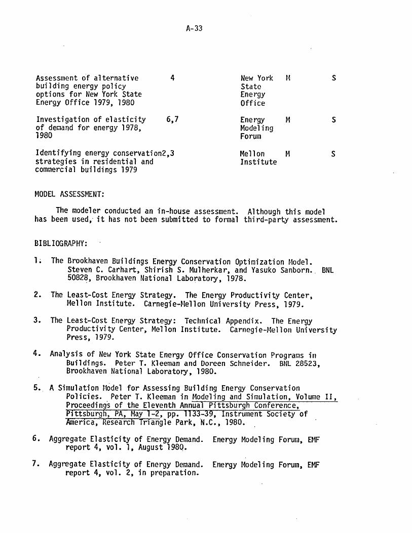
-- -- ~~~mi

A-33

Assessment of alternative 4 New York M Sbuilding energy policy Stateoptions for New York State EnergyEnergy Office 1979, 1980 Office

Investigation of elasticity 6,7 Energy M Sof demand for energy 1978, Modeling1980 Forum

Identifying energy conservation2,3 Mellon M Sstrategies in residential and Institutecommercial buildings 1979

MODEL ASSESSMENT:

The modeler conducted an in-house assessment. Although this modelhas been used, it has not been submitted to formal third-party assessment.

BIBLIOGRAPHY:

1. The Brookhaven Buildings Energy Conservation Optimization Model.Steven C. Carhart, Shirish S. Mulherkar, and Yasuko Sanborn. BNL50828, Brookhaven National Laboratory, 1978.

2. The Least-Cost Energy Strategy. The Energy Productivity Center,Mellon Institute. Carnegie-Mellon University Press, 1979.

3. The Least-Cost Energy Strategy: Technical Appendix. The EnergyProductivity Center, Mellon Institute. Carnegie-Mellon UniversityPress, 1979.

4. Analysis of New York State Energy Office Conservation Programs inBuildings. Peter T. Kleeman and Doreen Schneider. BNL 28523,Brookhaven National Laboratory, 1980.

5. A Simulation Model for Assessing Building Energy ConservationPolicies. Peter T. Kleeman in Modeling and Simulation, Volume II,Proceedings of the Eleventh Annual Pittsburgh Conference,Pittsburgh, PA, May 1-2, pp. 1133-39, Instrument Society ofAmerica, Research Triangle Park, N.C., 1980.

6. Aggregate Elasticity of Energy Demand. Energy Modeling Forum, EMFreport 4, vol. 1, August 198Q.

7. Aggregate Elasticity of Energy Demand. Energy Modeling Forum, EMFreport 4, vol. 2, in preparation.

. ,

A-34ENERGY MODEL ANALYSIS PROGRAM

I n,: -cy Lo:,l'oryl-.;achlr.ftls In!,lu : fe Ichnolo)y

cf3m~:-nrde. FMassachselts 02139

OUESTIONNAIRE FOR ENERGY POL'ICY MODELERS

The'M.l.T. Energy Model Anilysis Program (EMAP). under spon'.orship from the Electric Power Research Institute, is developinga directory of enrgy rroadels and assessrmen!s. to be pubtised In the la!l of t'30 The directory will be distributed w:dety togovernment d-pr:rnen's, academiz cst,:ut:on, and pr:vate 1n'dlus!ry. and wll be an extremely useful relerence tool for modeldevelopers, assessors. and users. We %,.ould very much like to include your model in this directory, and therefore are requestingthat you comp'ete the 13o!!:*.,rg form to provide the informnation needed. VWe ,.ill then compile your responses into a standard-lied format. which sil be sent to you for review prior to pub.cation.

Please answer the questions below as completely as you can, we are r,3rticularly pleased to be able to present in this directorythe kind of meanir.gful and interesting incrmation and perspecti e that only modelers and model assessors themselves canbrovide. We are interested in any hing you have to offer about your model,and encourage you to use extra sheets of paper wherenecessary. If you are extremely short o tnime, please answer the questions marked with an asterisk." Martha Mason ind KellyMorgan of the EMAP will be happy to answer any questions and offer assistance, they may be contacted at (617) 253-8318.

Thank you for your assistance - the directory will not be complete without an entry on your model!

GENERAL INFORMATION

*1. What is the name of the model? Brookhaven Buildings Energy Conservation Optimization

Model"2. By what acronym, nickname, or other name(s) is It.known? BECOM

'3. Where, and under what auspices, was the model developed. Developed at Brookhaven National

Laboratory under contract to the U.S. Department of Energy, Division of Buildingsand Community Systems.

*4. Over what time period was the model developed? mo 1/77mo /yr.

to 1/78moJyr.

*5. Who Is the person filling out this questionnaire?

Name: Dr. Peter T. Kleeman

Address- Building 475 , Brookhaven National Laboratory, Upton, NY 11973

Telephone 1(56) 3L5-2116

Retationsh;pto madet Have used and modified model for expanding its capabilities.

*6. Who is (or are) the key modeler contact(s)?

Name: _ _Dr .ter T. Kleeman Name: Chip Balzer

Address: Bldg. 475, Upton, NY 11973

Telephone. (516) 345-2116

Relationship to model: as above

Address: Bldg 4 5Upton, tY 11973

Telephone: (516) 345-2256

Relationshipto model: Data base and model maintenance

*7. Who is (or are) the key contact(s) in the organization(s) that sponsored the model development?

Name: Mr. Peter Back Name Mr. Steven Lee

Address. U.S. DOEC ashington, D.C. 20585 Address: U.S. DOE, Washiinston. D.C. 20585

Telephone: .1202 252-9426 Telephone: (202) 252-9426

Relationshtp to model.Jprr am sponsor Relationship to model: Program sponsor

MODEL CHARACTERISTICS

The following questions are designed to provide understanding of the fundamental technical characteristics of the model. Themultiple-choice options are provided for your convenience; however, we understand that models vary significantly, and thesechoices may not be suited to your model. Please add categories, phrases, or sentences, as applicable.

In Question 18 we ill ask about different operating versions of the same basic model. If there has been more than one version,please indicate here which one you are describing. If the versions are significantly different, you may find it necessary to fill outa complete questionnaire for each unique model version.

*8. What keywords characterize the Issues the model addresses?

O p)ply of fuels & resources & Econoic impacts of energy policiesWDemand lor e!eclrcity O Environmental impacts of energy policies

pemand for non-clectric energy P/Demographic/social impacts of energy policiesP. egulatory behavior L New technoloy assessmentDElectric utility behavior ;Conservation assessment "DOther industry behavior

2biher(s,eicty) Federal energy policy assessment

I'. What analylltc l,chniques are used in th, model? (if rpproprlate, check more then ons, and Indicate which subsection ofthe modal uses which technique)

b'Lnear picgrarn.nnin - Descriptive simulation]Nonlnealangr programming O Allocaton & equilibrium-Other slatic ophlmzatlon 0 Input/outputD 0yna.m c Cepltmiaton 0 Regress,on. economotric

.Stochastic techn-ques 0 Export opinion, non-quant:atlive

Olther (specify) _ ~C- ----

_____ __ ______~ --

A-35'10. a) What geographic resolution does the model cover?

1 te-sprhc,f¢ (Dsecily),wOget.: (-,-flPCIfy) _ _ fr__. U . _ .S._US_ _ ...T_C. ...

1, Statc.wadr+(,ls p, ct)ly)

US asawd,;,o'e as unioL. __iLour reg itons(. Inerna on.ld(pectdy)(U Other ('.b,acufy) _b) It regional information is aggregated before reporting results, what is the level of aggregation?

*11. a) What temporal resolution does the model cover?

_. ,hrl term (5 y,'as or less)t( /editrn term ('-20 years)O Long t!rm(over 20years)b) It there are discrete lime steps, what is their typical length?

12. Aside from their use as inpu, were data used during calibrationfdevelopment of the model?

yes - no (skip to ques. 13)II yes, how were the data used?

C tor coethlcientlparametet determinationo fot structural form determirat:on[0 for assessing the accuracy of model results0 other(specty)

*13. In the space below (or on extra sheets) please provide a cdmplete technical description of your model, discussing whenapplicable:

* model s!ructure and methodology * variables (endogenous & exogenous)"* signithcant equations * input data* oarameters * butpul data

When discussing input data, please differentiate between those data that serve as input assumptions imbedded in the model andthose that are frequentiy chang.d during model runs.

Please attach a flow chart or other d;agram of the structure of the model, if possible.

see attached report (reference 1 in bibliography)

--- ~- ----- --- -- --- ~~... YIYIIIII

A-36

114. The following questions cnncern the computing eiivironmont required by thu model.

a trani o!r chi:try ... Crntr rol )a a. Crp._CDC_7600b. Larigua, . ) -r, eoyeddPr;; /MAGLl '.EX.-C ,pp ,o,rr.ate CO.t pI)rr so!uthnn Co; _ .$5 _ Or tle.: _ per solutiond. Is the rrro.I I vrned wth oth.r mod.lts or soll;ware paCk:;ls'9

fo _XX Yes(r.pcly) Qrookiaven_ nerg y__Syn-_pt.mtimiza yel_ IqESO'Le Is the code alvaable on tape .yX __ cards y.__f. Are any Sarts of the model proprietary)

..X._No Yes(specly)

15. Bibliography

We would I ,e to snclud-, a bib:ihgraphy for your model Therefore. In the folow.ng space, or on an attachd sheet. please tst allreferences ni which the model has been described or cited. inciuding documentation. journals, publications, and reports on modelapplicatiors Please number each item for easy reference later in the questionnaore

1. The Brookhaven Buildings Energy Conservation Optimization Model. Steven C. Carhart,

Shirish S. Mulherkar, and Yasuko Sanborn. BNL 50828, Brookhaven National Laboratory,

1978.-

2. The Least-Cost Energy Strategy. The Energy Productivity Center, Mellon Institute.

Carnegie-Mellon University Press, 1979.

3. The Least-Cost Energy Strategy: Technical Appendix. The Energy Productivity Center,

Mellon Institute. Carnegie-Mellon University Press, 1979.

4. Analysis of New York State E~rl'-gy Office Conservation Programs in Buildings. Peter T.

Kleeman and Doreen Schneider. Nf, 28523, Brookhaven National Laboratory, 1980.

5. A Simulation Model for Assessing Building Energy Conservation Policies. Peter T. Kleeman.

in lodeling and Simulation, Volume 11, Proceedings of the Eleventh Annual Pittsburgh

Conference, Pittsburgh, PA, May 1-2, pp. 1133-39, Instrument Society of America,

Research Triangle Park, N.C., 1980.

6. Aggregate ElasticityAugust 1980.

7. Aggregate Elasticityin preparation.

of Energy Demand.

of Energy Demand.

Energy Modeling Forum, EMF report 4, vol. 1,

Energy Modeling Forum, EMF report 4, vol. 2,

16. Which documents listed in Question 15 are references for the model's data sources?Flelerencenumbers 1, 3.

A-37MODEL DEVELOPMENT AND APPLICATIONS

In this .ectlior we are interested in tracinr how th, riol-kt h~s been u.ed In the hr.t r.olornr. ple:ra,: duscrihe aclh anpplcatin ofthe lOd:!l, ustes might incluce both academic stdy ;aid .p,-cthc proublan r.olvarorj in the following colurns, pl.atre al,'Ciclttewhich reflerence numrib-r from Oue;tion 15 describ s the appl'ration, wtr the sponsor wvs lfor ttht application, who actuallyoperatd the model, and who suggested or su.pleed the scenrarios Implemented an the ar'pcdaton

Model Scenarios*Descripton of each sign;ificant Ref. # from Sponsor' operated supplied

apphicatior of the model. Ovestion 15 client by: by:including dates of usage: describing for each M= modeler M= modeler

each applic. applic- S= sponsor S = sponsoration ation O- other O other

Assessing market potential work is American Cas M Sof gas powered air-cod. currently in Association,technologies under various progress Arlington,VAfuel and technology priceassumptions 9/80 - pres.

Assessment of alternative 4 New York M Sbuilding energy policy State Energoptions for New York State OfficeEnergy Office

1979,1980

Investigation of elasticit 6, 7 Energy M Sof demand for energy Modeling

1978,1979 Forum

Identifying energy 2, 3 Mellon S S

conservation strategies Institutein residential andcommercial buildings

1979

17. As the table above suggests, an important factor in model development and documenta:ion is whether or not the modelhas ever been installed and operated by someone other than the modeler.

a) Can the model be transferred for use by someone other than the modeler?XxXYes No If no, why not?

b) Has the model ever been transferred for use by someone other than the modeler?XX No Yes If yes. please indicate where the model was transferred and briefly describe the

transfer process. _Sansoar..usedJ.L istjllatiat.._hutw~o d ~nden

C) Do you have any plans to transfer the model in the future?_.XX No . Yes if yes. towhere?

18. One factor sometimes complicating model assessment Is that one-time or on-going changes.to a model's structure haveled to more than one version of that modal. In this question we are Interestedin finding out how many discrete versions ofthe model have been developed, end which, if any, are current!y operational.

a) Has the model undergone any major structural changes since Its original finished forml.No(skip to Oues 19) .. X..Yes If yes, please briefly describe any sannthcant clrferences between the versions and

the reasons mc::va,!r gbe c, r5--s

b )Worunder. .tve ..namre of.c.t lLelto iuwhere r thtl .a o atory

b )Which version(s) of the model are currently operetional, and where are they maintained?

----------. I Y

A-38t.IODEL ASSESSMENT

*19. Ha> 11 fmodel over bCHert -ljRLlchd to an ill house assessment by the modolers?

4No('. p to Oir-s 20)

-- Yes a) If yes, which elements listed below received emphasis during the modeler assessment?0 Model vahai:y [U Usability

[ Structure Ll Documcntation.1 Conten! 1 Elliciency

0 Prediction 0 ModelC Data valtdly app!ications0 Veriication of the CJ Other (specify)

model's expres=ionin the computercode

b) Please briefly describe the techniques utilized in the modeler assessment.

*20. 1la- the model been made available for assessment by external parties?

( No (skip to Ojeshon 21)U) Yes. through pt.bcaton of model descriptions in the lihterature0 Yes. through a formal eterrial assessment- Yes. Vttrough ot hor means (specify)

II the model was assessed by an itdividual, group or organization other than the modeler(s), please answer the questions below:

a) Who was the assessor for the model?

OrganizationName of contact-.TitleAddress

Telephone( )Title of Report

b) Who sponsored the assessment?

OrganizationName of contact-Title _Address

Telephone( )

c) What assessment approach(es) were employed by the assessoes?

O Review of the litera;ure, not including the computer code0 Evaluation of the detailed documentation, including the codeo Audt of the model's performance. using test problemsO Evaluation of the model u .rg experiments designed by the assessors, but implemented by the modelers

] INrdepth assessment, in v,hich the assessors themselves implemented experimental runs of the model

C Comparative evaluat-on of two or more modelsSOtlher (specify)

d) Which elements listed below received emphasis during the external assessment of the model?

O Model vatidity 0 Usability0 Structure 0 Documentationo Content 0 Efficiencyo Prediction E Model

O Data validity applications0 Verification of the 0 Other (specify)

model's expressionin the computercode

e) Do you have any comments on the external evaluation of the model?

.21. a) Please discuss the accessibility of the model for initial or further assessment. If the model has not been assessed, do

you have any plans concerning future assessment? Do you feel it should be considered for an assessment?

ThjTsoodel is not_ agood candidate for assesssment since a mo.el is currently_ ein

developed tLhai t.w111 -in. e-f fcct.replace-this. .model _uirh _one. of...sup eri r_quzali.t)t

-Th is-modrln---i ,- c-urrent ly-knovn-a- KR-1- nnd- mnny--be- imp emented -end-doeumei ted------

imrcrr-uicMhn -rthe-n exrsvever a t onhs.

22. We would be interested in any other aspects of the model that you would like to discuss. How does it compare with other

models in terms of structure or coverage? Were there any interesting ramifications resulting from use of tihe model?

This model indicated in several applications that aggressive policies on the

part of the federal govt. could encourage large energy savings in both residential

and conunercial sectors. The bulk of these savings would occur through building

envelope improvement rather than conversion device retrofit or replacement

when real fuel prices paid by consumers increases.

mlhIIM,

A-39

References

1. Jack Faucett Associates, Inc. TEC: Transportation EnergyConservation Model, Jack Faucett Associates, Inc., August 1979.

2. Energy and Environmental Analysis, Inc., Industrial Sector Technolo~Use Model (ISTUM): Industrial Energy Use in the United Syayes,194-ZUUU, Vol. .1, EEA, Inc., June 19/8.

3. Carhart, Steve C. The Least-Cost Strategy--Technical Appendix(Carnegie-Mellon Unvirsity Press), 1919.

4. Conversation with Samir Salama, Harold Kalkstein, and Tim Hogan,Energy and Environmental Analsyis, Inc., May 29.

5. Conversation with Mike Laurence, Jack Faucett Associates, Inc., May29.

6. Telephone conversation with Barbara Richardson, University ofMichigan Highway Safety Research Institute, June 16.

Massachusetts Institute of Technology

Energy Laboratory

Energy Model Analysis Program

Appendix B

An Evaluation of the Mellon Institute

Least Cost Energy Strategy

by

George Tolley*Ronald Krumm *Edward Mensah*

June 1981

*Department of Economics, University of Chicago

Table of Contents

Introduction and Overview B-1

Market Adoption in the LCES B-2

A. Industrial Sector Analysis B-3

Market Share Projections B-4

Results B-7

Evaluation B-8

B. Building Sector B-16

Model Formulation B-17

Results B-17

Evaluation 8-18

C. Transportation Sector B-21

Model B-21

Results B-21

Evaluation B-22

Summary and Suggestions for an Improved Methodology B-25

I 1

B-i

INTRODUCTION AND OVERVIEW

The Mellon Institute Least Cost Energy Strategy (LCES) is an at-

tempt to examine how the effects of higher world energy prices

can be partially mitigated through the introduction of more efficient

technologies. The approach taken in the LCES is to consider competition

between alternative new technologies to determine their adoption patterns.

Very detailed breakdowns according to technology type, and energy service

demand by industry, transportation, and housing sectors are provided.

The scenario explicitly considered by the LCES is what technologies

and energy inputs would have been adopted in 1978. Actual energy service

quantities in 1978 are determined and then, not allowing for changes in

these quantities, the cost savings associated with adoption of least cost

technologies to meet these these energy service quantities are determined

using existing, large scale computer algorithms for each of the industrial,

transportation, and housing sectors. The industrial sector analysis makes

large use of the Industrial Sector Technology Utilization Model which is

not part of the LCES report but was partially available to us for exami-

nation. The building sector analysis relies heavily on the Building

Energy Conservative Optimization Model and the transportation sector

relies on the Transportation Energy Conservation Model. Documentation

of neither of these models was available to us for evaluation. Below,

our evaluations of the LCES are presented based on the LCES reports and

other limited material available to us but not included as documentation

to the Mellon Institute reports.

B-2

MARKET ADOPTION IN THE LCES

The methodology employed in the LCES is to consider energy'efficiency

improvements in three sectors of the economy: industrial sector, build-

ings sector, and the transportation sector. While improved efficiency in

each of these sectors had been substantial up through .1978, as pointed out

by the authors of LCES, the approach taken by them is to consider more

completely further efficiency improvements and the potential cost-savings

associated with their adoption. The question they wish to provide in-

sights on is "How would the nation have provided energy services in 1978

if its capital stock had been reconfigured to be optimal for the actual

1978 energy prices?" In essence, their answer to the question involves

comparison of costs of providing energy services among alternative techno-

logies in various sectors of the economy. This section examines the me-

thodologies used in this attempt and evaluates them in the hope of pro-

viding a more appropriate approach.

B-3

A. Industrial Sector Analysis

The first step in analysis of the industrial sector is to determine

the quantity of energy services demanded to produce given output levels

based on actual 1978 levels of economic activity. Given these quantities

as inputs, the Industrial Sector Technology Utilization Model (ISTUM) is

used to calculate the lowest cost combination of fuel and efficiency

improvement technologies to meet these quantities demanded. The average

cost of fuel prices in 1978 were used in this cost determination approach.

No changes potentially induced by lower cost alternatives, on economic

output levels or the distribution of economic activity are permitted.

Turnover of the capital stock in which technologies are embedded includes

equipment used in generation or conversion of energy but not other items.

The exercise considers 23 energy service sectors (e.g., machine

drive, space heat,etc.) in 26 industrial catagories. Within each service

sector technologies were adopted on the basis of the ISTUM lowest service

cost algorithum. The least cost estimates are based on an assumed con-

stant (1978 actual) quantities of service demanded and energy prices

through the year 2000, but allow for full turnover of energy using durable

goods taking into account replacement through the year 2000. The authors

suggest that limitations in the approach such as process changes due to

changing costs of energy services are not serious because the analysis

is only for one year, 1978. Numerous technologies are considered for

each of the 23 service sectors with competition between technologies

conducted separately for each service sector.

-- --- --- ---- EllL

B-4

Market Share Projections

Market share projections in the LCES are determined by use of ISTUM.

The discussion presented here is based in large part on documents referred

to in the LCES pertaining to ISTUM but not developed by the LCES. The

basic approach is to characterize the cost of a technology in terms of

capital costs and costs associated with the utilization of the durable good

in generation or conversion of energy services. With different costs

associated with alternative technologies and utilization rates the ob-

jective is to determine the least cost technology that would be adopted.

The cost of each technology is determined by adding up (using a discounted

cash flow technique) capital costs, fuel costs, and operating and main-

tenance costs. That technology with the lowest total cost is then the

appropriate technology to be adopted.

The procedure to determine the total cost associated with each

technology is to assume distributions of fuel costs, capital costs, and-

operating costs. For a particular type of plant this includes site pre-

paration, start-up costs, and other capital costs as well as refined

breakdowns for operating and maintenance costs. Appropriately, ISTUM

realizes that these costs may vary by plant for a variety of reasons

(included are site-specific valuations and firm-related variation).

Hypothetical ranges associated with cost variation due to these factors

are then used to deter-mine distributions of costs associated with all

factors that figure into total cost determination. These distributions are

then added together (assuming independence) to arrive at total cost dis-

tributions for each technology. Each technology is assumed to have a

I ---- _~_Mik

B-5

maximum market share in each service sector with some technologies excluded

(zero market share). The exact procedure for this determination, however,

is not explicitly addressed in the available documents. In addition to

these considerations, often some technologies are limited in application

because of restrictions in size either because of technical factors or

through regulation. The cost associated with a particular technology may

also depend on the extent of utilization. Thus load factor categories

are used within each service sector in analysis of competition among

alternative technologies.

Competition between alternative technologies is examined in five-

year intervals (1980-2000) with only those technologies available in a

given year able to compete. Thus, for example, a technology that is

expected to be developed in 1985 will have no effect on the technologies

available in 1980 and adopted in 1980. The nominal market share is

"...that fraction of the market segment in which that technology will be

able to supply energy to the final process more cheaply than any other

competitor."

Since the nominal market share determines the fraction of the

market in which any technology is theoretically preferable to any alter-

natives, based on the cost of the alternatives, it is most probably the

market ceiling for the particular technology. It is realized that the

acceptance of a given product or process in a market place is not

dependent on cost considerations alone. Factors such as consumer risk

aversion, lags in transfer of information concerning the technology,

role of governments, etc., all affect the rate at which a product/process

is adopted.

B-6

In the original industrial sector technology utilization model (ISTUM)

these factors are termed behavioral lag factors. ISTUM defines behavioral

lag as the amount of time in years required for actual market shares to

equal the nominal market shares (the market ceiling). It is supposed to

be a time lag function controlling the rate at which the actual market

shares approach the market ceiling. ISTUM concentrates only on costs and

does not consider the effect of net benefits of a particular technology

on its adoption. To get around this point, the ISTUM methodology uses

the ratio of the nominal market share (NMS) to maximum market fraction

(MMF) as a measure of the perceived profitability of a technology (PTP)

and in turn the expected length of the behavioral lag. The assumption is

that the higher this ratio, the higher the perceived profitability of a

technology and hence the shorter the behavioral lag time.

The behavioral lag time (BLT) is modeled as the product of the

initial technology behavioral- lag time, ITBLT, and the behavioral lag

multiplier. The ITBLT is defined as the maximum number of years one

could imagine that risk aversion and information transfer constraints

which delay the commercial acceptance of a product/process could be over-

come. ISTUM sets the upper limit of this number to be 15 years.

A risk aversion multiplier (or lag time slope) is defined as the

slope of a downward sloping straight line which depends on the nominal

market share relative to the maximum market fraction. This slope is

set equal to 5.0. After calculating the behavioral lag time for each

technology, the actual market share (AMS) is computed according to the

B-7

following procedure:

0, where t - YTA < 0

AMS = NMS(t) x (t - YTA(t)), where 0 < t - YTA(t) < BLT(t)

NMS(t), where t - YTA(t) > BLT(t)

where YTA = Year technology is available

BLT = Behavioral time lag

t = Time in calendar years

The assumption is that once time t exceeds the year technology is

available, (YTA), by the technology behavioral lag time, actual market

share will be equal to the nominal market share. Since this model does

not take into consideration the probable appearance on the market of

more superior technologies, it is not clear whether the nominal market

share or the market ceiling will ever be approached by most of the

technologies.

Results

In the industrial sector, technological improvements in energy ef-

ficiency accounted for 22% of the industry energy service market in 1978

in the absence of least cost strategy. However, the results also show

that if least cost strategy had been applied in 1978, technological

improvements in the energy efficiency would have accounted for 33% of

the energy service market. Oil utilization in industry contributed to

18% of the energy service market in 1978 and in the hypothetical situation,

oil would have accounted for only 11% of the energy utilization in indus-

try. Another important difference in energy utilization in industry was

__ __ /1

8-8

in the area of natural gas usage. The results show that while natural

gas accounted for 22% of the energy service market in 1978, if least cost

strategy had been employed natural gas would have accounted for 37% of

the energy service market in 1978. Purchased electricity would have

captured 11% of the market for energy services in industry in the presence

of least cost strategy in 1978 but the actual share of the market captured

by purchased electricity in 1978 was 26%. Industrial coal utilization

would have dropped from 10% in the actual 1978 situation to 7% in the

hypothetical case.

On the whole, energy cost per capita which was $257 would have de-

creased to $232 if least cost strategy had been employed in 1978. This

is a 10% drop in the actual 1978 situation.

Evaluation

Table 1 presents the major comments of our evaluation of the LCS

modeling effort.

First, the modeling effort provides a detailed breakdown of

energy service demand sectors and industrial catagories. This disaggre-

gation effort is an important step forward in analysis of market adoption

of new innovations. They have provided a model that brings to light some

of the effects of competition between new technologies on the extent of

adoption which are essential ingredients in understanding adjustment

to the changing world energy situation.

Second, the demands for energy sources in each sector are assumed

fixed at their 1978 levels, not responsive to price or expected growth

B-9

TABLE I

COMIMENTS ON THE LCES INDUSTRIAL SECTOR ANALYSES

1. The detailed breakdown of energy service demand sectors and industry

categories is a necessary step forward in the modeling of market

adoption of new technologies.

2. Effects of energy service cost reductions due to adoption of new

technologies on costs of outputs and input quantities demanded

need to be considered to determine total market adoption patterns.

3. The LCES results are relevant for comparison of cost savings asso-

ciated with adoption of new technologies only in the sense that they

compare actual costs to what costs could have been if adoption

of new technologies took place in a non-dynamic setting without un-

certainty. A more realistic approach is needed that takes into

account market adoption decisions in a world where future changes

in prices and economic conditions are uncertain.

4. Costs of adjustment are not explicitly modeled in the LCES market

adoption methodology. Factors that alter the rate of adoption of

new technologies should be viewed in the same manners as other costs

and explicitly included in the LCES analysis.

___ _ ~~ ~_ ~ ~ "L,,/

B-1 0

TABLE 1 (con'tl

COMMENTS ON THE LCES INDUSTRIAL SECTOR ANALYSES

5. The level of existing durable good stock structure, embodying older

technologies should be explicitly considered in the determination

of adoption of new technologies. Replacement of existing technologies

will depend on the age and efficiency structure of capital

goods in which technologies are embedded and thus will alter the

rate of adoption of a new technology depending on this structure.

6. Effects of expectations of introduction of newer technologies in the

future on current adoption patterns of new technologies in the current

period need to be explicitly treated in the LCES analysis. The age

structure of existing capital stock, the life terms of alternative

new technologies and the extent of expected future cost reductions

will play important roles in determination of market adoption pat-

terns of existing new.technologies.

7. The approach taken in the LCES through use of ISTUM is to consider

dispersion of elements of costs associated with purchase and utili-

zation of new technologies. The economic reasons for this disper-

sion need to be explicitly incorporated into the cost structure

analysis instead of relying on mechanistic procedures to determine

cost dispersion and the maximum market penetration of new techno-

logies. Variation in labor costs and other input costs as well as

output market conditions need to be included in a more complete

analysis.

B-11

TABLE 1 (con't)

CO4MENTS ON THE LCES INDUSTRIAL SECTOR ANALYSES

8. A least cost of production strategy could include substantial re-

location of industry to areas where fuel costs are lower and cli-

matic conditions are such to lower demand for energy servies in

heating and cooling capacities. However, the benefits to the pop-

ulation may be more substantially decreased because of higher costs

of transportation and/or costs associated with population relocation.

Instead of relying on cost of production decreases as the LCES, a

more appropriate approach would be to consider reduced costs of

population consumption of all goods and services.

9. The cost savings associated with adoption of a technology that pro-

vides two distinct services is the sum of the savings in each cate-

gory. The appropriate comparison between alternative technologies,

some of which provide multiple services, should take into account

such joint cost savings. The current cost comparison algorithms, to

the best of our knowledge do not take into account these properties.

10. The year of availability of new technologies, just like costs of

existing technologies, should be allowed to depend on economic factors.

-- --------- I Y

B-12

or decline in demand. Further, reduced costs of production in one

sector of the economy due to adoption of new technological innovations

do not affect production costs in other sectors. For example, reduced

steel prices would not reduce the cost of automobiles. People often

consume not the output of metal fabrication industries but rather services

from goods they directly purchase. A direct measurement of the benefits

to society of adopting new technologies is the ability of people to

purchase goods and services they directly consume and not the changes in

costs associated with intermediate goods used in production.

Third, although the LCES results are only meant to relate to what

happened in 1978 relative to what could have happened if the LCES were

followed, it is not clear that given the information available in 1978

and earlier, the LCES results may not have been appropriate, even with

perfect foresight with respect to new technologies. For example, great

uncertainty with respect to future energy prices may optimally lead to

less investment in new technologies that would have large benefits asso-

ciated with their adoption only if fuel prices did not decline.

Fourth, costs of adjustment are not explicitly treated in this

modeling effort. If all relevant capital was to turn over immediately

in 1978, the cost of producing all the durable goods that embody the new

technology may increase in cost. Thus the cost distribution associated

with supply of one type of technology will not be independent of the

quantity of other technologies supplied. More explicit treatment of the

aggregate implications of the model results and their appropriateness is

needed.

10 Iffi iiM ,

B-13

Fifth, the role of the existing capital stock and cost of utilization

relative to that associated with the new technologies needs to be more

completely developed. The efficiency of the existing capital stock may

depend significantly on its age structure and thus the technology imbedded

in it. It appears there is an asymmetry between competition between existing

(old) technologies and that between new technological innovations.

Our understanding of the model is that all old capital is replaced by

improved existing technologies as of 1978 and this old capital has no

value. An economic treatment of this subject would not lead to this

result and that it is not likely to be a least cost strategy. In order

to carry a more sound economic analysis along these lines it would be

necessary to compare costs of utilizing existing durable goods that

embody old technologies with both costs of new durable goods containing

new technologies and their costs of utilization.

Sixth, the expected introduction of a new technology in the future'

does not affect what technologies are adopted in the current period.

Even abstracting from the existence of current old technologies that are

in place, the choice between two equal-cost technologies available in the

current period,but with different lifetimes, will not be adopted at the

same rate if it is expected that in two years a new, dominant technology

will become available. In addition, in some cases it may be least costly

not to replace an old technology with a new, more efficient technology,

if it is expected that an even more efficient, less costly technology

will be developed in the near future. These trade-offs need to be more

explicitly dealt with in the Mellon Institute study.

B-14

Seventh, the approach taken in the LCES through the use of ISTUM is

to consider dispersion of elements of costs associated with the purchase

and utilization of new technologies. The economic reasons for this dis-

persion need to be explicitly incorporated into the cost structure analysis

instead of reliance on mechanistic procedures. For example, variation in

labor costs and other input costs will alter the variation in cost in a

systematic manner that should be included in the cost structure analysis.

Eighth, a least cost strategy could involve the relocation of all

industry to regions where energy costs are minimized and/or where cli-

matic conditions are such as to require very little heating services. This

may lead to very low costs of production but an overwhelming decrease in

the benefits that stem from the consumption of the goods purchased. In

other words, the resulting increase in costs of transporting goods and

services where people live would outweigh the savings achieved by pro-

duction relocation. Moreover, such considerations suggest that the effects

of energy cost changes in production and distribution' (the transportation

sector) cannot be developed independently. Optimal adjustment to higher

energy prices thus involves comparison of both benefits and costs asso-

ciated 'with the adoption of new technologies in a spatial context.

Ninth, the cost savings associated with adoption of a technology

that produces two distinct services is the sum of the cost savings in

each category. The appropriate comparison, for adoption purposes, between

technologies that have such characteristics should take into account these

joint cost savings amounts. The current cost comparison algorithms, to

the best of our knowledge, does not take into account this property.

B-15

Tenth, the year of availability of new technologies. depends on dif-

ferences between regions, prices, labor ayailabilities, site-specific

factors as well as qualitative service demand differences such as pro-

duct/process reliability. The model should include the effects of inter-

actions between these factors on the availabilities of new and improved

technologies and make new technology development a result of economic

determinants.

-- YYI

B-16

B. Building Sector

The LCES for the building sector focuses on the lowest cost combina-

tion of energy technologies that would satisfy the actual 1978 quantities

of a variety of service demands. Nine building types were considered

under the residential and commercial building categories; the residential

category had four building types--single-family detached, low density,

multi-family, and mobile homes. The commercial buildings category is

made up of the following: office, retail, school, hospital, and miscel-

laneous. Service demands in a building category are broken down into

four types: 1) space heating, 2) air conditioning, 3) thermal demands

(water heating, cooling, drying), and 4) lighting/appliances.

An example of a space heating demand for a single-family house is the

energy required to maintain a reference house, defined explicitly in

terms of its thermal characteristics, at a reference temperature for

one year. Fuel demand is then derived from service demand by adjusting

for fuel conversion efficiences.

Service demands were derived for new and existing buildings for each

of the four end uses--space heating, air conditioning, thermal, lighting/

appliances--in each of the nine building types in the four specified

regions of the U.S. The LCES uses the Building Energy Conservation

Optimization Model (BECOM) which derives the least cost mix of capital

and fuel required to meet all service demands. However, no documentation

of this model was available.

B-17

Model Formulation

The model is formulated as a trans-shlipment problem with energy as

the commodity to be shipped from the supply nodes (fuel sources) to the

demand nodes (building service demands). All the possible ways of satis-

fying the service demand for each building type in each region are

specified. Each procedure is likely to incur a different cost. The

components of the costs are 1) fuel cost, 2) capital cost amortized

over the lifetime of the equipment, and 3) the capital cost of the

structural improvements, also amortized. The costs are represented as

costs per unit of service adjusted for efficiency.

Given the efficiencies of the equipments and the structural tech-

nologies and the associated costs, the preferred mode for the provision

of a service demand is one that provides the energy service at the lowest

cost. A discount rate of 5% is used in the LCES. The model is basically

a cost minimization linear programming algorithm which seeks to achieve

the least cost of provision of a specific level of service demand in a

given building type in all four regions of the U.S.

Results

According to the LCES modeling effort, building energy service markets

would have shown a 23% reduction in the cost of energy services per capita

if the least cost strategy had been employed in 1978. Technological im-

provements in energy efficiency accounted for only 2% of the energy service

market in the building sector in the actual 1978 situation. But in the

least cost case , a hypothetical 1978 case, improvements in energy effi-

ciency would have contributed 35% of the market for energy services.

~~----- .~-- ---- --------- IUii

B-18

The shares of oil, natural gas, and purchased electricity in the

buildings' energy service would have declined if least cost strategy had

been followed in 1978. Oil would have accounted for 12% of the building

sector energy service market in the hypothetical case compared to 16% in

the actual 1978 situation. The share of natural gas in the energy

services market would have decreased from 56% in the actual 1978 situa-

tion to 37% in the hypothetical situation.

Intensive retrofitting of residential and commercial structures

would have been mostly responsible for the differenc between the two

cases, contributing to over 8% of the aggregate energy service market.

It was also found that under the 1978 hypothetical case, the introduction

of more energy-efficient appliances would have occurred.

Evaluation

Table 2 gives our major comments on the LCES modeling in the building

sector.

First, regional representative technologies are described in much

detail for all building types. Most of the refined breakdowns deal with

alternative technologies and associated costs. This is a necessary first

step in analysis of adoption of alternative technologies in the housing

sector.

Second, documentation of the procedures used in the LCES is not

complete so that comment on the underlying determinants of market pene-

tration cannot be clearly presented.

miiiM 01 lu

B-19

Third, homogeneous conditions are assumed within each broad regional

category although very substantial variations in climatic conditions,

structural characteristics, and energy prices exist. A need is to

consider more completely this intra-regional variation in the above

factors.

Fourth, the 1970's were characterized by substantial regional and

intra-regional change in location of population. To the extent that

differential energy costs played a role in these patterns, market

penetration results in the buildings sector may not affect the least

cost strategy.

Fifth, similar to the modeling for the industrial sector, no con-

sideration is given to the role of existing technology age structure, or

age structure of the housing uinit itself. Issues associated with adoption

of new technologies in existing buildings need to be examined more com-

pletely before the LCES results can be useful in describing potential

cost savings.

Sixth, sensitivity analysis with respect to assumptions made would

be useful in establishing the stability of the results and indicating

which assumptions need to be more fully addressed.

B-20

TABLE 2

COMMENTS ON THE LCES BUILDING SECTOR ANALYSI.S

1. Very refined breakdowns of alternative technologies are presented

and provide a necessary first step in market adoption analysis.

2. Documentation of analytical procedures used limits comment on the

methodology.

3. More refined intra-regional breakdowns would enhance the usefulness

of the modeling effort.

4. Substantial movement of population between and within regions in the

period analyzed needs to be included in the analysis of housing demand

and associated energy use.

5. The role of age structure of existing housing stock and technologies

needs to be more fully incorporated into the new technology adoption

process.

6. Sensitivity analysis to the assumptions made would be useful in

indicating which assumptions need to be more fully explored.

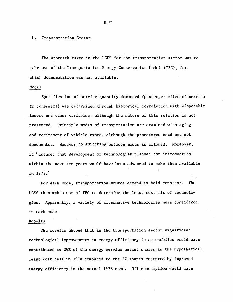
B-21

C. Transportation Sector

The approach taken in the LCES for the transportation sector was to

make use of the Transportation Energy Conservation Model (TEC), for

which documentation was not available.

Model

Specification of service quantity demanded (passenger miles of service

to consumers) was determined through historical correlation with disposable

income and other variables,. although the nature of this relation is not

presented. Principle modes of transportation are examined with aging

and retirement of vehicle types, although the procedures used are not

documented. However,no switching between modes is allowed. Moreover,

it "assumed that development of technologies planned for introduction

within the next ten years would have been advanced to make them available

in 1978."

For each mode, transportation source demand is held constant. The

LCES then makes use of TEC to determine the least cost mix of technolo-

gies. Apparently, a variety of alternative technologies were considered

in each mode.

Results

The results showed that in the transportation sector significant

technological improvements in energy efficiency in automobiles would have

contributed to 29% of the energy service market shares in the hypothetical

least cost case in 1978 compared to the 3% shares captured by improved

energy efficiency in the actual 1978 case. Oil consumption would have

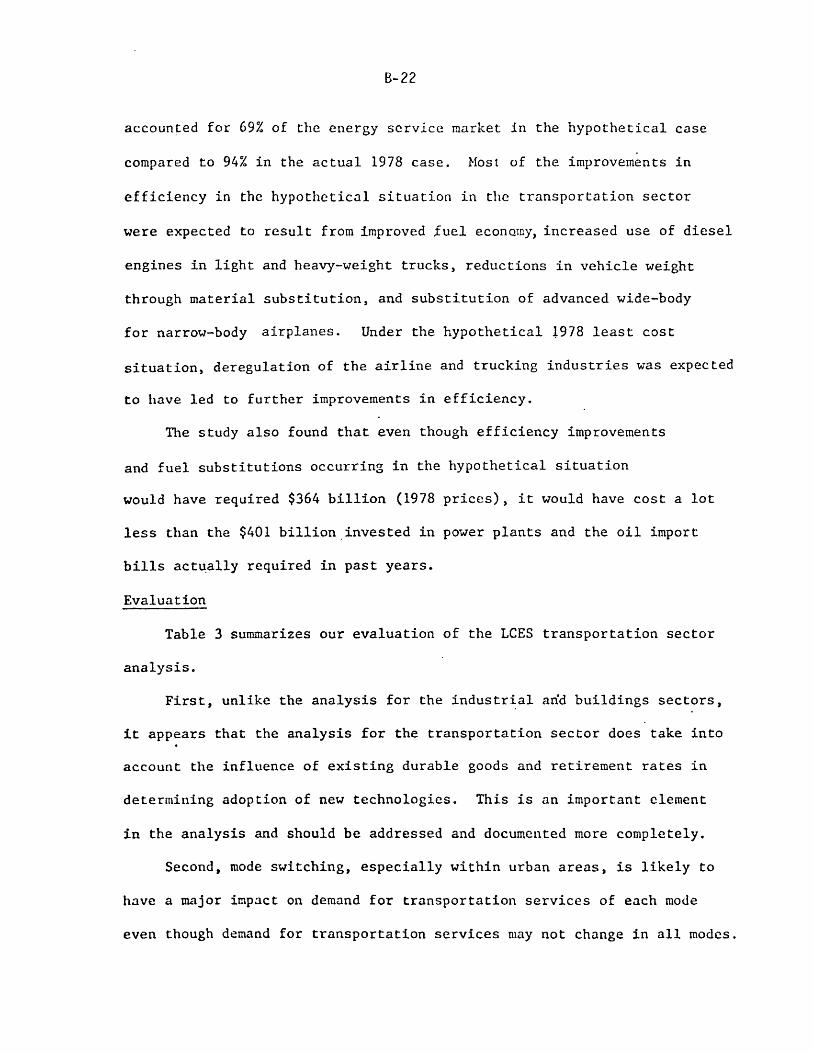
B-22

accounted for 69% of the energy service market in the hypothetical case

compared to 94% in the actual 1978 case. Most of the improvements in

efficiency in the hypothetical situation in the transportation sector

were expected to result from improved fuel econemy, increased use of diesel

engines in light and heavy-weight trucks, reductions in vehicle weight

through material substitution, and substitution of advanced wide-body

for narrow-body airplanes. Under the hypothetical 1978 least cost

situation, deregulation of the airline and trucking industries was expected

to have led to further improvements in efficiency.

The study also found that even though efficiency improvements

and fuel substitutions occurring in the hypothetical situation

would have required $364 billion (1978 prices), it would have cost a lot

less than the $401 billion invested in power plants and the oil import

bills actually required in past years.

Evaluation

Table 3 summarizes our evaluation of the LCES transportation sector

analysis.

First, unlike the analysis for the industrial add buildings sectors,

it appears that the analysis for the transportation sector does take into

account the influence of existing durable goods and retirement rates in

determining adoption of new technologies. This is an important element

in the analysis and should be addressed and documented more completely.

Second, mode switching, especially within urban areas, is likely to

have a major impact on demand for transportation services of each mode

even though demand for transportation services may not change in all modes.

I IY1 - __ .. IId hYYI

B-23

TABLE 3

COMMIENTS ON THE LCES TRANSPORTATION SECTOR ANALYSIS

1. The role of age structure and retirement rate associated with existing

durable goods is included in afalysis of new innovation market penetra-

tion, but needs to be more completely documented.

2. Mode switching as a result of changing costs needs to be included in

the analysis as it has been found in a variety of studies of nrban

travel demand to be an important element in transportation analysis.

3. Effects of transportation cost changes on location of population and

production need to be addressed.

4. More complete documentation of effects of environmental and govern-

ment regulatory activity on the transportation sector should be in-

cluded.

" I IN I IIIIIINI iimlmmmll0IM 1 'llY II "

B-24

Mode switching due to cost changes has been well-established in studies

of urban areas and needs to be included in the LCES modeling effort.

Further, the historical correlations used to determine mode demand should

include such interactions.

Third, transportation costs have played an important historical role

in determination of location of population and jobs. Regional growth and

change as a result of transport cost changes is not included in the

modeling effort but is likely to be a long-term result.of such transpor-

tation cost changes, thus altering regional demand for transportation

services. A need is to more fully develop these issues in a least cost

energy modeling effort.

Fourth, environmental factors and government regulatory changes

have been included in the model and are likely to be of substantial

importance. However, to evaluate precisely the effects of these con-

ditions on penetration of new technologies a more complete documentation

is necessary.

B-25

SUMMARY AND SUGGESTIONS FOR AN IIPROVED METHODOLOGY

The Mellon Institute study is an attempt to examine how effects of

higher world energy prices can in part be lessened by adoption of more

efficient technologies that compete with each other on a cost basis. The

economic basis for these adjustments is recognized by the LCES but rigorous

economic analysis of the adjustment process is seriously lacking in the

LCES modeling effort.

The mechanistic approach taken by the LCES needs to be altered so

that the underlying economic principles affecting market adoption of new

technologies is explicitly included in the process of adjustment to chang-

ing world energy process. Serious analysis of this adjustment and the pro-

cess of new technology adoption must address the manner in which existing

and new technologies embedded in durable goods compete both at any point

in time and over time.- Such analysis needs to he based on a framework

that considers relationships among the level of adoption of alter-

native technologies and the rate at which these change. -In essence, mar-

ket adoption of innovations is a dynamic process that must he examined in

that context, including uncertainty with respect to future conditions.

Market adoption patterns of a single new technology will depend on how

costs and benefits of adoption of that technology over time are related to

costs and benefits of adopting alternatives. over time and the replacement

process now and in the future. The mechanistic algorithms used in the

LCES are not sufficient to accurately reflect the complicated dynamics of

change involved. In addition, analysis of market adoption of new techno-

logies must be viewed in a setting of a dynamic economy with changes in

industrial composition and location of production and population in addi-

tion to changes in world energy prices.

11W IIIIII d11 11 11 WNIWN -- 0 I1

Massachusetts Institute of Technology

Energy Laboratory

Energy Model Analysis Program

Appendix C

The Least-Cost Energy Strategy and the Economics of Cogeneration

Alan J. Cox*

June 1981

*The author is currently a student in the Graduate School of BusinessAdministration, University of California, Berkeley. This paper hasbenefited from comments by Ernst Berndt, Roger Bohn, Paul Joskow,Michael Manove, Fred Pickel and David Wood.

_- ---;;---^I--- -- _I ---TI---r;-;;l---rr=---eg ~__ _ __ ~Z

TABLE OF CONTENTS

Page

The Least-Cost Results C-2

Review of Least-Cost Strategy Procedure C-6

Technical Constraints Estimation C-8

Market Competition Analysis C-8

Capital Cost Issues C-20

Conclusions C-24

Appendix C.1 - Brief Review of Cogeneration C-26

Steam-Topping Technologies C-26

Gas Turbine Combined Cycle C-38

References C-42

C-I

This paper is a review of the assessment of cogeneration in the

Mellon Institute Energy Productivity Center's report "The Least Cost

Energy Strategy" (the LCES Study). LCES results show far greater

penetrations of cogeneration than are found in other literature on the

subject. Some of these differences can be explained by merely examining

the input assumptions of the relative costs of investing in the various

cogenerating technologies and of the relative costs of fuels. However,

the biases that result from these assumptions can only be clearly

understood through a detailed examination of the methodology.

Cogeneration is conventionally defined as the joint production of

heat and electricity. The joint production can be thought of as reducing

the costs of producing each of the outputs through the "writing-off" of

part of capital and operating costs to each of the outputs. The costs of

producing electricity will then be the residual of the net cost of

producing steam, or the cost of producing steam can be the residual of

the net cost of producing electricity.

The plan for this paper is, first, to compare the LCES results with

those found in other reports. The input assumptions that lead to the

divergence of the LCES results from the other reports are reviewed

briefly. The methodology of the LCES report is then reviewed in some

detail. That description, drawing heavily on documentation provided by

the creators of the model utilized for tile LCES report, is followed by a

discussion of the estimation of the capital costs of cogeneration. The

emphasis in that discussion is on the problems of trying to predict the

total of individual investment decisions using aggregate energy demand

data. The purpose of that discussion is not so much to criticize the

model, which in many respects is satisfactory, but to outline the

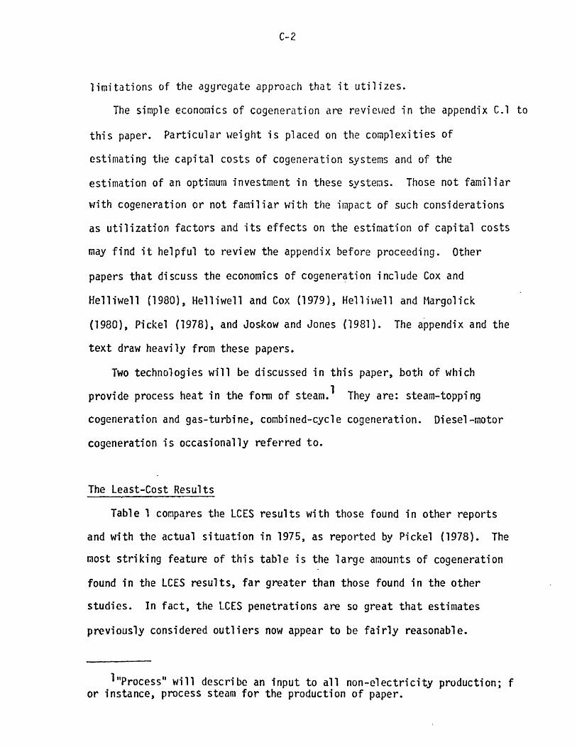
C-2

limitations of the aggregate approach that it utilizes.

The simple economics of cogeneration are reviewed in the appendix C.1 to

this paper. Particular weight is placed on the complexities of

estimating the capital costs of cogeneration systems and of the

estimation of an optimum investment in these systems. Those not familiar

with cogeneration or not familiar with the impact of such considerations

as utilization factors and its effects on the estimation of capital costs

may find it helpful to review the appendix before proceeding. Other

papers that discuss the economics of cogeneration include Cox and

Helliwell (1980), Helliwell and Cox (1979), Helliwell and Margolick

(1980), Pickel (1978), and Joskow and Jones (1981). The appendix and the

text draw heavily from these papers.

Two technologies will be discussed in this paper, both of which

provide process heat in the form of steam. 1 They are: steam-topping

cogeneration and gas-turbine, combined-cycle cogeneration. Diesel-motor

cogeneration is occasionally referred to.

The Least-Cost Results

Table 1 compares the LCES results with those found in other reports

and with the actual situation in 1975, as reported by Pickel (1978). The

most striking feature of this table is the large amounts of cogeneration

found in the LCES results, far greater than those found in the other

studies. In fact, the LCES penetrations are so great that estimates

previously considered outliers now appear to be fairly reasonable.

l"Process" will describe an input to all non-electricity production; for instance, process steam for the production of paper.

111W11

C-3

TABLE 1

Estimates of Congeneration Penetration

Total U.S. cogenerated electricity as apercentage of total electricity productiop,1975 (Pickel, 1978)

Massachusetts estimate of profitable cogenerationin state as a percentage of 1977 electricityconsumption. Base Case. (Massachusetts, 1978)

Resource Planning Assoc.1

Dow (1975)1Thermo-Electron (1976)1ISTUM1

Least-Cost(a) 2

Least-Cost(b)3

1 As percentages of 1985 demand projected by DRI.(1978) using 65 percent utilization rate.

4%

19%

5.5-16.4%

18.2%7.7%5.9%

51 .6%37.7%

Adapted from Joyce

2 Industrial cogeneration as a percentage of 1978 industrial demand.Estimated from gas consumption figures. Table III.3.3of LCES technicalappendix. Total gas use for electrolytic and machine drive demand = 2.95Quads. At 60% efficiency this gives 1.75 Quads of electricity.Percentage cogeneration is then (1.75/(2.21 +.1.18) where 1.18 isindustrial demand for purchased electricity.

3 Total cogeneration as a percentage of total 1978 demand. Estimated asin (a) plus oil consumption for diesel cogeneration in buildings times40% efficiency. Oil use in diesel cogeneration in buildings (from Table111.4.1) 2.29 Quads. At 40% efficiency, this gives .916 Quads ofelectricity. Total electric purchasesdf LCES study is 4.4 Quads. (1 .75+ .916)/(1.75 + .916 + 4.4) = .377.

C-4

This is not the only unusual result. The LCES report shows all

industrial cogeneration coming from gas turbine systems. This result is

not found in any other study and is not even found in the original report

on ISTUM, the computer model upon which tile LCES industrial results were

based and which is described below. Table 2 has been drawn up to

indicate this divergence. It presents two estimates of the fuels

consumed in the production of steam and cogenerated electricity by

predicted levels of investment in different technologies. The fuel

consumption figures are in percentages. Each percentage is the

proportion of the total fuel consumed to meet either steam or electricity

demand. The first of these results is from the original report on

ISTUM. The second set of results is the LCES result. The fuel cost

input assumptions are also listed for both studies.

While gas turbines provide very little steam in the ISTUM study, this

technology provides almost half the steam in the LCES study and meets

about half the demand for electricity. Similarly, while coal provides

large amounts of steam in the ISTUM study and some electricity, it

provides none of either in the LCES study.

The major reasons for these results were found to be:

i) The low price of natural gas assumed in the LCES study, a price

consistent with the average price in 1978, but not representing its true

value as a substitute for oil, nor its likely level in the gradually

deregulated future. Natural gas is the presumed fuel for gas turbines in

the LCES study, while ISTUM assumed the turbines to be fired by oil.

Thus, the cost of fuel for the gas turbine is $2.50/MMBtu for ISTUM and

$1.55/MMBTU in the LCES study.

ii) Capital costs were generally found to be understated in the LCES

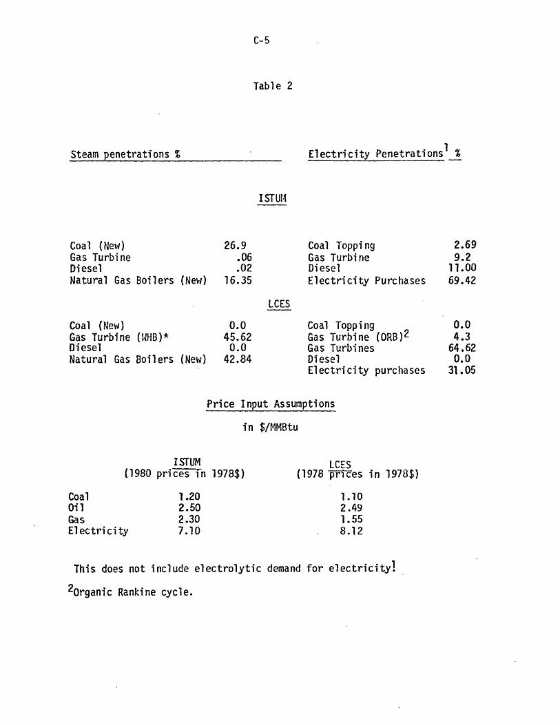
I iIII

C-5

Table 2

Steam penetrations %1

Electricity Penetrations _%

I STUI

Coal (New)Gas TurbineDieselNatural Gas Boilers (New)

26.9.06.02

16.35

Coal ToppingGas TurbineDieselElectricity Purchases

LCES

Coal (New)Gas TurbineDieselNatural Gas

(WHB)*

Boilers (New)

0.045.620.0

42.84

Coal ToppingGas Turbine (ORB)2

Gas TurbinesDieselElectricity purchases

Price Input Assumptions

in $/MMBtu

ISTUM(1980 prices in 1978$)

LCES(1978 prices in 1978$)

CoalOilGasElectricity

1.202.502.307.10

1.102.491.558.12

This does not include electrolytic demand for electricity!

2 organic Rankine cycle.

2.699.2

11.0069.42

0.04.3

64.620.0

31.05

C-6

study, with the exception of coal boilers, which were assumed to be about

twice as expensive as their current cost.

The primary consequence of this particular set of assumptions is that

investment in gas-turbine technologies are made to appear cheaper than

investment in steam-topping systems or to purchasing electricity.

However, gas turbines produce about four times as much electricity per

pound of steam than topping technologies. Thus, the apparent biases in

the cost assumptions lead to the choosing of a technology that produces

far more cogenerated electricity than found in other studies.

To see the manner in which these input assumptions affect the choice

of technology and the amount of cogeneration it is necessary to review

the methodology employed in the LCES paper.

Review of Least-Cost Strategy Procedure

The model upon which the Least-Cost Energy Strategy report depends is

an adaptation of ISTUM, which itself was developed for DOE and is

documented in Department of Energy (1979). Figure 1 is a flow diagram

that illustrates some of the steps in this process. The model takes as

inputs fuel prices, technology capital costs, and energy demand data. It

evaluates a set of technologies to find the combination of them that

meets fixed energy service demand at lowest cost. The penetrations of

some technologies are limited by technical constraints. "Energy demand"

is separated into 26 industries, each with up to 23 energy service

demands. Two of these service demands are relevant to cogeneration;

machine drive demand and steam demand. These services are the only two

that will be considered in this review.

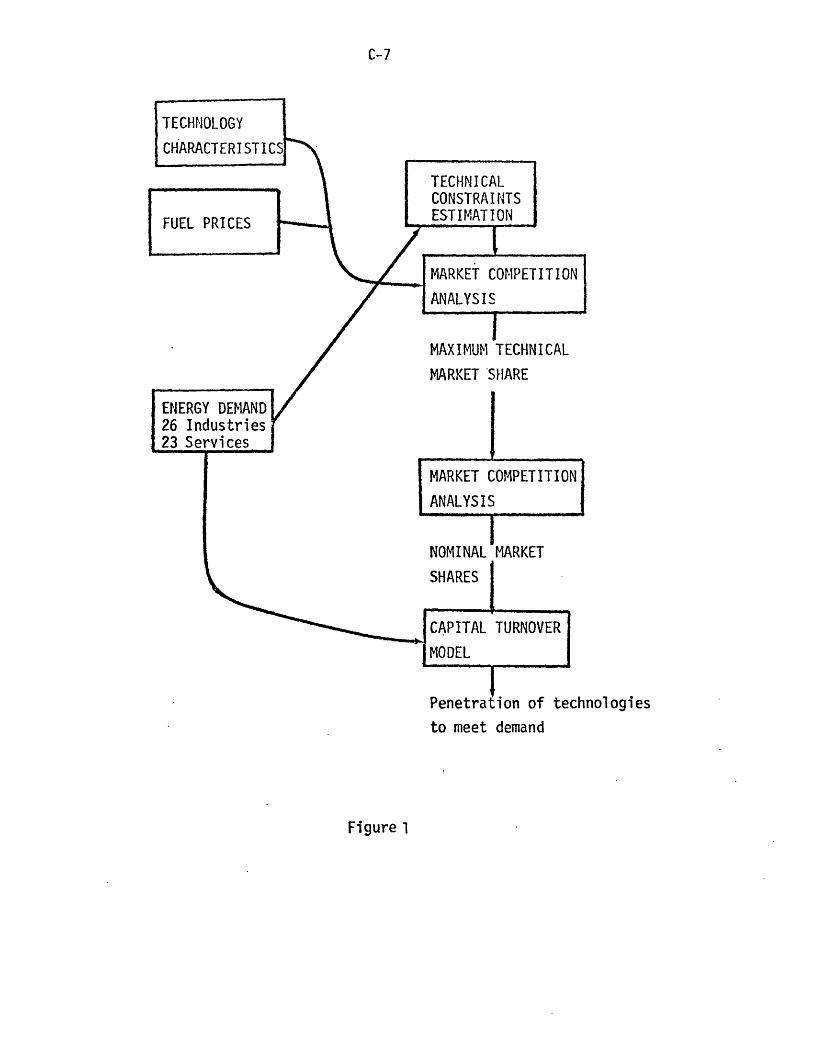
C-7

MAXIMUM TECHNICAL

MARKET SHARE

ENERGY DEMAND26 Industries23 Services

MARKET COMPETITION

ANALYSIS

NOMINAL MARKET

technologies

to meet demand

Figure 1

.I h

C-8

Technical Constraints Estimation

Cogeneration systems can only produce a certain number of kWh per

pound of process steam demand. For instance, a steam-topping system with

a boiler pressure of 1250 p.s.i., a heat content per pound of steam of

1375 Btu, and a process requiring steam at 150 psi, can produce about 55

kWh of electricity per thousand pounds of steam generated to meet process

heat requirements. The steam-topping maximum market share is estimated

as:

STt C,t PT Pg (-h 3 ) (1)ST,t M (1)Tt

where ST, t is the maximum share of machine drive energy demand

that coal-topping can meet,

MC,t is the total amount of new coal-fired boiler capacity

installed in year t, in Btus,

MT,t is the total demand for electricity, in Btus.

PT' Pg are turbine and generator efficiencies (pT . pg = .7), and

&h3 is the change in Btus per pound of steam as it expands

through the turbine, as a percentage of Btu/lb, as steam

exhausts the turbine.

This can be converted to an equation to estimate the amount of

cogeneration potential available in kilowatts by replacing MTt with

3412, the number of Btus per kilowatt hour.

Market Competition Analysis

ISTUI takes the costs of providing an energy service from the range

of possible technologies and picks the lowest cost system to meet that

demand. However, instead of using point estimates of the cost of each

. . .II ll YI lI ,,

C-9

technology's services (which would result in a single technology

capturing the whole market or up to the maximum allowed by its technical

constraint) the model utilizes a range of per-Btu costs for each of the

technologies.

The costs of meeting steam- and machine-drive service demands through

cogeneration are estimated in two inconsistent ways. To understand this

problem it is helpful to review the capital costs involved in

cogeneration systems.

The major investments that are incremental to providing steam and are

due solely to the decision to cogenerate electricity from a steam topping

system include :

i) the cost of the turbo-generator,

ii) the cost of the additional boiler capacity necessary to produce

the greater output of steam necessary to make up for the heat

converted to electricity,

iii) the additional boiler cost resulting from a boiler of a

pressure higher than that necessary to provide process steam alone,

if the investor is considering increasing cogeneration capacity in

this manner, and

iv) the cost of any condensing capacity.

While the isolation of the incremental cost of producing electricity

from a coal topping cycle is straightforward, the same cannot be said of

the other two technologies. In fact, both diesel and gas-turbine

cogeneration could be considered primarily electricity-generating

technologies, with steam being a by-product. However, the ISTUM

methodology requires that these technologies compete in well-defined

service sectors, either steam services or electricity services. All

C-10

three technologies must first.compete to meet industrial steam demand.

The capital costs of meeting steam demand with a coal system is merely

the cost of a conventional coal boiler. However, the cost of providing

steam from the gas turbine and diesel technologies is deemed to be the

total cost of the systems, minus the benefits to the firm of producing

electricity for its own use and for sale to the local utility. The

average cost of providing process steam fom a gas turbine could then be

represented as

AC = (K + FS + FT - BE)/Btu (2)

where ACS is the average cost of a Btu of steam,

K is the total annual capital and operating cost,

FS is the cost of fuel consumed to raise steam to meet process

heat requirements,

FT is the additional fuel required to produce electricity from

any steam topping system,

BE is the annual benefit due to reduced electricity purchases

and due to sales of surplus electricity, and

Btu is the annual process heat production.

Thus the greater the price of electricity the lower is the cost of steam

used in production. Also, the lower the cost of the fuel burned to

produce both steam and electricity, the greater will be the net benefits

of producing electricity and hence, the lower will be the cost of

producing steam.

Coal boilers with no cogeneration capacity then compete with

gas-turbines and diesel cogenerators to meet steam demand on the basis of

their average costs of steam. Once the amount of steam generated from

gas turbines and diesels is estimated, the amount of electricity produced

C-11

can be computed. This electricity production is then subtracted from

that required by the machine drive sector. The remaining machine drive

demand is met by steam topping and purchased electricity, whichever is

cheaper.

Thus, three cogeneration technologies are evaluated in two

contradictory ways. The ISTUM modelers no doubt felt that, since there

was no way to isolate a steam-producing segment of the gas-turbine system

or the diesel system, they had to think of the steam generating

investment as being incremental to the electricity generating system.

However, it is incorrect to assume that the incremental cost of producing

electricity is embodied in one technology. Consider the case of a plant

manager evaluating the purchase of a new steam generating system and

faced with the choice of the three technologies. The cheapest way to

produce steam alone will probably be the coal system since the other two

systems produce the steam merely as a byproduct. Suppose the manager

then considers the possibility of cogenerating electricity. The

incremental cost of cogenerating by steam-toppping is, as we saw, the

additional boiler cost plus the cost of turbo-generator. The incremental

cost of producing electricity from a gas-turbine or a diesel system would

be the total cost of those systems, minus the total cost of the coal

boiler large enough to provide steam requirements alone. In this manner

all technologies could compete on the same basis in order to meet

electricity demand.

Conversely, the method applied by ISTUMt for gas turbines and diesels

(equation 2) could be applied to the coal-topping system as well. The

credit to be applied to the cost of process steam production would be the

value of electricity produced.

C-12

Once the net steam costs had been evaluated for all possible topping

designs this technology could compete with gas turbine or diesel

cogeneration systems on the same basis. This sort of approach has been

suggested by the developers of the ISTUM model. (See Olson and

Kalkstein, 1980.)

Even if these methodologies had been applied consistently to all

technologies, however, it is unlikely that they would result in an

optimum investment strategy. The only way to do that would be to

calculate the net present value of the whole range of possible technology

options, including conservation possibilities. More specifically, that

means subtracting the capital, fueloperating and maintenance costs for

the entire investment (i.e. not broken into their component parts) from

the present value of electricity savings. The project which supplies

steam requirements with the smallest negative value should be the one

undertaken. However, in a system that chooses technologies by minimizing

costs instead of maximizing benefits, such a procedure, though correct,

cannot be undertaken.

In summary, the amount of machine drive demand satisfied by each

technology is based upon each technology's penetration into the steam

market. The cost of steam from coal is merely the cost of a coal

boiler. The cost of steam from a gas turbine is the total cost of that

system, minus the benefits of electricity production. With the very low

prices for natural gas and the realistic prices for electricity found in

the LCES study the gas turbines take a very large share of the steam

sector market. The amount of electricity generation that this

gas-turbine steam penetration implies is so large that there is little

left for any other technology to capture.

C-13

To see how the results of Tables 1 and 2 come out of the LCES study

it is useful to look at the assumed capital and fuel costs for each

technology. The first part of Table 3 displays the LCES cost assumptions

(in dollars per MMBtu) for the technologies. It clearly demonstrates the

economic advantage that gas turbines enjoy under the LCES scenario. The

costs shown are after electricity benefits have been subtracted. The

electricity savings are somehow allocated over both the capital and fuel

costs of the gas-turbine system. In some cases the fuel costs are

reduced to a negative number. The credits earned from electricity

generation are $6.76/MMBtu for electricity (about 2.3V/kWh) and the cost

of the fuels are $1.55/MMBtu for natural gas and $2.49/MMBtu for

diesel. (The fact that the minimum costs under the "fuel" and "total"

headings are higher than their mean costs may indicate that the cost

distribution of the ISTUM system have been replaced by using the mean as

a point estimate.)

As Table 2 indicates, the natural gas price assumptions are clearly

very low, resulting in the low net fuel prices for gas turbines on column

3 of Table 3. The 1978 prices are much lower than those that one could

reasonably expect after natural gas deregulation. The LCES study implies

that investors will be very myopic in their decisions to invest in

cogeneration,even though the life of this equipment is very long.

What if potential cogeneration investors had not had as myopic a view

of the price of natural gas and expected to face the marginal cost of

natural gas by 1985? In the second and third sections of Table 3 are

represented some of the LCES cost assumptions adjusted to take into

account different possible prices for natural gas. In the second section

we add an additional $O0.75/MMBtu to the cost of gas to bring it up to the

C-14

Table 3

Technology CostsSteam Service

$/MMB t uLCES Cost Assumptions

From Table II 2.5

Technology

SteamGas TurbineNew Coal

Machine DriveCoal toppingPurchasedElectricity

SteamGas turbine

SteamGas tur!bineNew Coal

Machine DriveCoal topping

Capital + O&MMean Min

3.2 2.13.4 2.7

7.9 4.20.27 0.15

FuelMean Min

-.4 1.21.25 .97

1.8 1.47.6 1.5

TotalMean Min

2.8 3.34.7 3.6

9.7 5.67.87 2.8

ISTUM Price Assumptions

3.2 3.6

Deregulated Case Cost Assumptions

3.23.4

7.9

2.263.06

3.6

5.466.46

10.7

Corrected Coal Costs with Deregulated Fuel

SteamNew CoalMachine DriveCoal Topping

1.82 -

2.761

3.06

3.6

4.88

6.36

1 From page 11-98, Vol. 1 of ISTUM reported, corrected for differentinterest rates and for inflation.

C-15

ISTUM case. In that scenario the difference between the cost of steam

from a gas turbine and the cost of steam from a coal boiler is reduced

from $1.9/MMBtu to $1.1/MMBtu.

For a "deregulation" scenario all prices are set on the basis of the

cost of oil in 1980 when residual oil was priced at an average of

$4.27/MMBtu. Coal is assumed to have a long-run price of one half of the

price of residual oil. (It was actually about one third the price of oil

in 1980, but the one half proportion is closer to the historic

situation.) Natural gas is priced at 85 percent of oil. Under this set

of assumptions the cost of new coal steam is $1.00/MMBtu above that of

gas-turbine steam.

With these fuel cost adjustments the coal technology still costs more

than the gas turbine technology but the reduction in the differences

between the mean prices could well have resulted in some coal being used

to generate both steam and electricity. However, a further adjustment

must be made to the LCES cost assumptions. The assumptions of investment

costs for coal systems are too high. The discrepancy between the LCES

assumptions and currently listed prices is discussed below, under

"Capital Cost Issues." Corrected coal cost estimates are listed in the

last section of Table 3. The additional adjustment to capital costs

results in the cost of coal being below that of the gas turbine in

providing steam.

The annual holding cost of capital utilized in the LCES study is also

too low. The LCES formulation for estimating the annual cost of capital

includes no consideration of taxes and assumes a discount rate of 5

percent. Even if the discount rate were acceptable, the inclusion of

taxes would almost double the cost of holding capital. Since gas

---~ YYYYII.YY

C-16

turbines have a higher capital cost than coal boilers, this correction

would make gas-turbines even less attractive for the production of steam.

With fuel and capital costs adjusted to be more realistic, the LCES

results would have shown far greater production of steam from coal

boilers. The biased input assumptions combined with the ISTUM

methodology result in the gas turbine technology capturing most of the

steam market. With less gas-turbine steam production, far more of-the

machine drive demand would have remained to be competed for by

coal-topping cogeneration and by purchases. Furthermore, coal-topping

would not have captured as high a percentage of electricity demand. With

the cost assumptions of the last row of Table 3 coal would have captured

a substantial portion of this market. The appendix and the capital cost

section contain discussions of the reliability of these cost estimates.

Electricity Prices and Utility Operations

The electricity prices used are about the same as the average U.S.

industrial price in 1978. A valid objection to the use of these prices

lies in considering the relative costs of capital to the utility and the

potential cogenerator. Utilities clearly expect a higher rate of return

than the 5 percent real rate enjoyed by the LCES investors and pay some

taxes that are not accounted for in the LCES study. A more reasonable

(i.e. higher) cost of capital faced by cogenerators would reduce the

amount of cogeneration in the LCES study. On the other hand, the average

industrial rate charged for electricity is based on the historic book

value of the utilities' capital stock. A socially optimal level of

cogeneration can only be found if the price of electricity is based on

the costs of new capital to utilities. In most cases this would result

_ IM._

C-17

in a higher price of electricity and, therefore, increased cogeneration.

Any study that purports to estimate the socially optimum mix of energy

technologies should do so on the basis of the marginal costs of all

energy, including the marginal cost of electricity.

Furthermore, the estimate of the marginal cost of electricity should

take into account the large amounts of cogeneration that are being

projected. There are two primary concerns of having large amounts of

generation connected to the utility grid but not under the control of the

utility; the reliability of the dispersed systems and the effect on these

systems on operating costs.

Figure 2 outlines a simplified flow structure for modeling these

effects. A utility's hour-by-hour demand for electricity is collapsed

into a cumulative distribution of demand (referred to as a Load Duration

Curve) which is then fed into a production costing model. The minimum

cost of meeting the demand for electricity is estimated taking full

account of the reliability of each unit owned by the utility. The

overall reliability of the system is also measured. The operating costs

are passed on to a rate-setting model which utilizes infomnnation on the

investment history of the utility to estimate regulated rates and also

calculates rates based upon the long-run marginal costs of the

utility.2 Both sets of rates should be used to compute the level of

cogeneration; one in response to current regulatory practice, the other

in response to socially optimal prices.

The amount of investment in cogeneration should provide a time

profile of the production of cogenerated electricity which can be

2 Both sets of rates include prices of electricity both for sale andfor purchase by the utility.

Figure 2

MODELING SYSTEM

Utility COGENERAT ION

Rates INVESTMENTRate Setting MDModel MODEL

C-)-!

C-19

subtracted from the original load duration curve. The new load-duration

curve is then run through the production costing and reliability model

and the rate-setting model. Depending upon the effects of cogeneration

on net load, the operating costs of meeting the new demand will be less

than, equal to, or greater than during the first iteration. A revised

set of rates is then estimated to pass on to the cogeneration investment

model, revised levels of cogeneration investment are calculated, and a

new load duration curve is fed back into the system.

No work has been done to examine the effects of large amounts of

cogeneration on the operating and capital costs of a utility. Work

reported in Cox (1981), Tabors, et al. (1981) and Finger (1981) on the

effect of large amounts of photovoltaic producers connected to the

utility grid indicate that, for this technology, the operating costs of

the utility are reduced. As more and more electricity is fed into the

grid the utility shuts down some of its most inefficient plants. With

increased penetration of these dispersed generating systems cheaper and

cheaper electricity is displaced. Thus additional dispersed units

provide lower benefits.

The strong correlation between peak demand and maximum photovoltaic

output (which may also exist between peak demand and maximum

cogeneration), allows the utility to reduce its capital requirements and

maintain its reliability requirements. On the other hand, Lee and

Yamayee (1980) predict increases in spinning reserve requirements with

levels of photovoltaic penetration greater than 6 percent of a utility's

peak demand.

Either increasing or decreasing costs to the utility through large

penetrations of decentralized generation will result in a reduced value

IYIYII

C-20

for cogeneration. Reduced total utility costs due to production savings

will be passed on as lower rates to customers reducing cogeneration

benefits. Increased costs (e.g., for spinning reserve) due to

cogeneration alone will be assessed against cogenerators and will also

result in lowered profitability.

On page 36 of the summary LCES report, gas turbine cogeneration is

shown to save 1.6 percent of the 1978 U.S. energy consumption. This

result can be approximately replicated from the information provided in

the LCES technical report 3 . It is important to note, however, that the

LCES authors are implying a substitution away from oil, coal, nuclear,

hydro and some natural gas-fired utility generators. The savings are

thus not necessarily in oil and natural gas.

Problems with the the relative prices of electricity and natural gas

account for a large part of the surprising results of the LCES study.

However, the estimation of relative capital costs also has an impact on

both the choice to cogenerate and the choice of technology with which to

cogenerate.

Capital Cost Issues

The investment costs quoted in the ISTUM reports seem to be fairly

consistent with costs published elsewhere. A standard design for a 108

MW gas-turbine combined cycle system, according to Pickel (1978), costs

$455/kW. ISTUM uses a mean price of $444/kW (Vol 1, p. 11-99). Cox and

34.18 Quads of steam generated times .4562 of this steam comingfrom gas turbines times .82 Quads of electricity per Quad of steamproduced by gas turbines divided by 79 Quads of energy consumed in theU.S. gives .0198. To save 1.6 percent indicates that for every Quadburned to produce electricity by cogeneration a utility would have toburn 2.2 Quads.

C-21

Helliwell (1978) report an average capital cost of electricity production

of l.0/kWh (1978 Cdn. $) for cogeneration from wood-fired topping system

in British Columbia whereas the ISTUM document reports a capital cost of

.78/kWh (1978 US $) for coal-fired cogeneration. The LCES study seems

to have retained the same investment costs as those found in ISTUM for

the gas turbine systems. For instance, the ISTUMt report states a total

cost for gas turbines as $11.16/MMBtu, which, after subtracting fuel

costs gives $5.41/MMBtu. After correcting for changes in the fixed

charge rate used in the LCES study, the ISTUM result transforms to

$3.79/MMBtu. The equivalent capital cost quoted in the LCES study is

about $4.5/MMBtu. (This interpolates between two capacity factors

presented in the LCES study.)

There is one glaring inconsistency between the capital cost estimates

of the LCES study and the ISTU14 study; the capital costs of

coal-topping. An estimate of the mean cost of capital for this

technology in the ISTUM study (p. II-98 of Vol. I of Department of Energy

(1979)) is one half that found in LCES study. An overestimation of coal

capital costs was also found in the steam demand sector. Pickel (1978)

reports (on p. 217) that the cost of a typical field-erected coal boiler

is .0315 $/Btu/hr. For a 300 thousand pound boiler this coverts to about

$10.4 million (1975 $), which would be about $12.94 million in 1978

current year dollars. Assuming a load factor of .457, this gives an

annual cost of $879,160. The operating and maintenance costs for this

system with the same load factor would be $792,000. This becomes

$990,000 in 1978 dollars. Dividing capital, operating and maintenance

4 This conversion is made using the Handy-Whitman index of electricutility costs. See Whitman, Requardt and Assoc. (1980).

C-22

costs by the expected annual heat production gives $1.416/MMBtu. The

LCES study uses a value of $2.996/MMBtu for the same sized boiler,

utilized at the same 46 percent rate. Thus we find that coal consumption

is understated partly because the LCES workers utilize a cost that is

twice as high as that found in other reports.

There are, in addition, two issues in the estimation of capital costs

that neither ISTUM nor the LCES study take into account. These issues

are better addressed by studies that examine individual plants instead of

whole industries. Pickel (forthcoming) shows that past predictions of

cogeneration based on aggregate studies have overestimated the levels of

cogeneration. This is partly due to important details being excluded,

details that must be dealt with by surveying plants separately. Pickel

(forthcoming) and Helliwell and Cox (1978) show the advantages of this

approach.

The first of these capital cost considerations has to do with

economic retirement of older plants. ISTUM assumes that the rate of

retirement in the past will continue into the future. This is hardly a

reasonable assumption for energy generating and consuming equipment. As

an example, consider a plant with several boilers, and with annual

production expected to remain constant. Each time there is an increase

in energy prices a plant manager examines the stock of boilers, with a

view of replacing that equipment. If the present value of savings due to

the installation of a new, more efficient boiler is greater than the cost

of installing that boiler, then a new boiler should be purchased. Thus

the rate of replacement is a function of the rate of change of the

relative costs of energy and capital. If energy prices increase on a

sustained basis more rapidly than they have in the past, then replacement

C-23

rates will be greater. As the ISTUI4 documentation states, these factors

are not taken into account (Vol. 1, p. IV-103). The data upon which the

retirement rates are based are ten five year periods from 1926-1975.

Thus, the data on retirement rates are based on a period of decreasing

real costs of energy, except for the last 5-year observation.5

Premature retirements will impose additional costs on a firm. The

writing-off of large amounts of undepreciated capital, while having no

economic consequences, will have an impact on the fins ability to raise

the capital necessary to make the economically efficient investment.

But the zero economic cost of discarding undepreciated capital is not

entirely a correct assumption to hold for cogeneration ihvestments.

Imagine a potential investor in cogeneration who has a boiler which

currently has 10 years of economic service remaining. An estimate of the

net benefits of adding cogeneration equipment to the current boiler

indicates that the project would result in losses. A possible

alternative is to scrap the boiler for one designed to provide more

electricity per pound of steam or to invest in a gas-turbine system. In

this case, the cost of cogenerating electricity must include the value of

the discarded boiler in order to cogenerate electricity. Thus, the

prospect of producing electricity may result in early retirement of

capital, but the costs of such a retirement would tend to push the

retirement date back towards the date that it would have been retired had

there been no increase in electricity prices. These scrapping costs are

not taken into account in the ISTUM4 cost distributions. They probably

5 However, instantaneous and unexpected changes in the price ofenergy, spaced with intervals of real price declines will have no effecton survivorship rates. There will be rapid adjustments in the capitalstock with retirements proceeding at their previous rate.

ammggiglglmilgglhlI 1 Il ,1.1 l1ll li, i 11 W hI II II 1111 il l l umull l l l Ul m ll lM n llN

C-24

cannot be measured in an aggregate model of this sort, again pointing to

the preference to individual plant modeling.

The ISTUI4 methodology measures capital costs as a function of the

projected capacity factors of the equipment used. However the average

costs of energy from a new system may not be the same as the marginal

cost of producing energy from the total energy producing plant (i.e.,

with both old and new capital). With indivisibilities of capital and

economies of scale matched against continuous increases in steam demand,

a firm will purchase equipment in such a way that some of its capital

will be redundant. Thus, some investments that may seem attractive on

the basis of the average cost of energy with a fixed capacity factor will

not be so when the marginal cost of energy production is used as the

investment criteria.

In addition to the problems of indivisibilities it is important to

consider the complexities of the cogeneration investment that are

outlined in the appendix. Firms faced with base load demand for steam

plus a highly oscillating demand above that base will not purchase a

cogeneration system to capture all of that peak, but may utilize an array

of technologies that will efficiently utilize the varying demand for

steam. The perspective of the individual investor is much different from

that implied by a model that optimizes upon a national steam demand. The

smaller systems that such considerations would lead to will also

significantly reduce efficiencies, particularly for gas turbines.

Conclusions

The results of the teast-Cost study indicate levels of cogeneration

far greater than those predicted elsewhere. The LCES study also

C-25

indicates that all industrially cogenerated electricity should ideally

come from gas turbine systems. The penetration of cogeneration is much

greater than even that found in the report of early results from ISTUM,

the model upon which the Least-Cost report is based.

There are four major weaknesses of the LCES study. The first of

these is the unrealistically low price of natural gas which fuels the gas

turbine technology. Secondly, this low price results in gas turbines

capturing a large share of the demand for steam, an outcome of the ISTUM

methodology which was found to be inconsistent in the way it treated

different technologies. The large amounts of cogeneration that the LCES

study predicts arise from this bias towards gas turbines because this

technology produces about four times as much electricity per pound of

steam than topping systems.

Thirdly, the large penetrations of cogeneration have profound

implications on electric utilities' costs of production. These issues

are not addressed anywhere in the Least Cost study.

Finally, capital costs of technologies were often incorrect.

The cogeneration submodel suffers from the problem of trying to model

very complex individual investments in an aggregated manner.

Considerations raised in this paper and in the appendix indicate that

such an effort is likely to miss key considerations that must be taken

into account and that will vary from plant to plant.

. . . .. YlIYI i i i II li III "

C-26

Appendix C.1

Brief Review of Cogeneration

Figure Al provides a diagramatic representation of the three

technologies discussed in this paper and which are described below. The

Least-Cost study also includes a fourth technology for on-site generation

of electricity, a gas-turbine combined with an organic rankine cycle.

This technology produces electricity only, and will not be discussed.

Steam-Topping Technologies

The standard method of producing steam for process requirements is to

combust fuel below a boiler in which steam is raised. In order to assure

a constant supply of steam, the boiler pressure is significantly greater

than that which is required at the process site. The steam can be passed

from the boiler through a pressure-reducing valve to the production site

where it is required at from 60 to 150 pounds per square inch (p.s.i.).

As heat is transferred to the production site the steam condenses and is

pumped back into the boiler.

Electricity can be jointly produced with steam by dropping the

steam pressure from boiler to process through a turbine attached to a

generator. The energy cost of producing this electricity is only the

energy loss in converting the stea into electricity in the turbine. At

a typical electric utility plant a considerable amount of energy is lost

to the environment in order to condense tilhe steam after it leaves the

last turbine. With a cogenerating system the heat loss in condensing is

actually recovered in the production site. What otherwise would have

been a heat loss can be thought of as being written off as a cost of

producing the plant's non-electric output.

Steam turbine STEAM TURBINE COGENERATION

r Electric power

cGeinrat-i I E,

Feedwater

Fuel Stack

Wasteheatboiler

GAS TURBINE COGENERATION

Gas turbine

Process steam

Feed water

) Electric power

Stack

DIESEL COGENERATION

Air

Fuel

Diesel engine

Process steam

Feedwater

Electric power

Generator

Figure A-i Schematic of Cogeneration Technologies

StackC-27

Steam

Air

~--- ~ ~ I'INHUHII .

C-28

The amount of electricity that can be produced by cogenerating is

limited by the demand for steam and by the temperature and pressure drop

across the turbine. (See equation 1.) For a given steam flow,

therefore, the amount of electricity cogenerated at a particular site can

be increased by building a boiler of greater pressure and temperature.

Figure A2 shows a transform from steam demand to electricity

cogeneration potential. (Equation 1 is the exact formula for the

transform.) Figure A2a represents a hypothetical steam demand for a

plant over one year. This demand shows seasonal fluctuations but assumes

the hour-to-hour demand to be constant.

Figure A2b represents the same steam demand of the plant as a

cumulative distribution. It expresses the probability that any level of

steam demand, in thousands of pounds per hour, will be experienced by the

plant at any point in time. Figure A2c is the cumulative distribution of

possible cogenerated electricity production that arises from the steam

demand of Figure A2a, assuming the same set of boiler and process

pressures and also assuming the installed capability to harness all the

cogeneration potential. This capability includes, as we see later, the

existence of excess capacity in the boiler.

Thus, at an installed cogenerating capacity X* kW, the plant will be

able to fully utilize the turbo-generator 50 percent of the time and will

be able to produce, per year, a number of kilowatt hours equal to the

area under the curve below X*AB times 8760, the number of hours per year

(see Figure A2c).

The components of the capital costs of cogenerdting by steam-topping

vary with the exact configuration of the system. One possible design

would size the boiler(s) to be just large enough to provide the maximum

steam demand

103 lbs/hr

steam demand

103 lbs/hr

-0

0.cr C"

cogeneration potentialkW

6Z-3

SWCD

r

C-30

steam necessary for all non-electricity production. Since some heat

energy is converted to electricity, this heat must be made up with

additional steam from the boiler over that required for non-electrical

production. If the boiler is just large enough to provide peak process

steam demand then no energy will be available for electricity production

during periods of peak process requirements.

Figure A3 shows the derivation of the cumulative distribution

function of cogeneration capability for such a system. In Figure A3a we

again show a seasonally fluctuating demand for process steam. The shaded

area indicates the amount of steam available for cogenerating

electricity, with the maximum steam available for cogeneration, H',

occuring during some summer hour. Figure A3b shows the cumulative

distribution function for process steam demand. Figure A3c is the

cumulative distribution for electricity that can be generated from the

steam available in the shaded area.

The depiction in Figure A3 implies that there is enough turbine

capacity to convert all excess steam to electricity by cogeneration. If

this is not the case then excess steam is used for cogeneration until the

maximum amount of electricity production is attained. At that point

total steam demand continues to go down at about tile same rate as process

steam demand.

This situation is depicted in Figure A4. The result of this

situation is a flat portion of the cumulative distribution function for

electricity generation. This sort of profile and distribution function

would result if the potential cogeneration investor wanted to improve the

utilization of the turbo-generator even though process steam demands

would allow higher amounts of cogenerated electricity.

I --;I-. --------- Ylliil

C-31

steam demand

103 lbs/hr

steam demand

103 Ibs/hr

cogeneration potentialkW

tio -

0U-

CD

-v0COCT7

'i mhIIIIY I M IIm I li ll

steam demand

103 Ibs/hr

cogeneration potentialkW

-3n),

0

_.j

4 9

cC

C-33

If the plant designs that gave rise to Figures A3 or A4 were

employed, the additional capital cost of producing electricity would be

merely the cost of the turbo-generator alone since the boiler(s) would

have been necessary for process steam requirements. Tile total production

of electricity and, hence, average cost of capital per kilowatt-hour of

electricity would depend upon the number of hours that the boiler would

have spare capacity. The percentage utilization will also depend on

the size of the turbine generator. The larger the turbine, the fewer will

be the number of hours during which there will be enough spare boiler

capacity to use the turbo-generator to full capacity.

A profit-maximizing firm would probably find the design strategies

discussed above to be sub-optimal if they provide any profit at all.

Larger turbo-generators could be built and their utilization could be

increased by building a larger boiler and continuously feeding some steam

to the production site through the turbine. The degree of utilization

would depend upon the size of the boiler and of the turbine. These

systems relax the constraint of steam availability and are faced with

only the constraint of a sufficient heat sink at the production site for

cogeneration to take place.

Figure A5a shows, as a solid line, the process steam;i demand of Figure

A4a. The vertical distance between the solid line and the dashed line is

the additional steam necessary to make up the heat losses due to

cogeneration when all the cogeneration potential is utilized. The

vertical distance is greater during the winter due to the large potential

available at that time. Figure A5b translates the total steam production

into a cumulative distribution function for steam demand; Figure A5c

illustrates the transformation of steam demand to a cumulative

1_ ~_^_ *11 li~ I-- YIIIYIIYII ,.ri

O

D

01

01-vocaf

0

Cr

C-34

steam demand

103 lbs/hr

,steam demand

103 lbs/hr

cogeneration potentialkW

-------- ____________*YiImmrnii

C-35

distribution of cogeneration potential. The peak cogeneration potential

is greater than that depicted in Figure A4 because the steam producing

capability of the boiler has been removed as a constraint.

The utilization of both the turbo-generator and the boiler can be

improved by reducing the capacity of both. This is depicted in Figure A6.

For the situation in which only excess steam demand is used to

produce electricity the only capital cost of cogeneration.is just the

cost of the turbo-generator. With some steam always being made available

for cogeneration there is added a second component of the capital cost,

the cost of building a boiler of capacity greater than that required for

process requirements alone.

There is an additional incremental cost that can arise in

steam-topping cogeneration. As noted above, more electricity can be

produced per pound of steam by using a boiler of a higher pressure ari

temperature rating at some additional cost. Furthermore, the bofier ifllf

have to provide more steam to make up for the increased energy Toss fn

the additional electricity production. These supplementary costs can be

partially offset against the economies of scale captured v4th', the l arger

boiler and turbo-generator.

A final possibility is the inclusion of some condensing capability to

the electricity generation equipment. This will augment the production

heat sink when the production demand for steam is low. Figure A7 shows

steam demand profiles for such a system. The shaded area in Figure A7a

is the additional capacity that is available for condensing generation.

The area between the solid and dashed lines of Figure A7a is the steamr

utilized for cogeneration, that below the solid line steam for process

requirements. Figure A7c shows the electricity production profile for

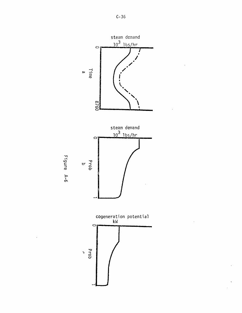
C-36

steam demand

-C

(D

C

a

-or ~

-5O

steam demand

cogeneration potentialkW

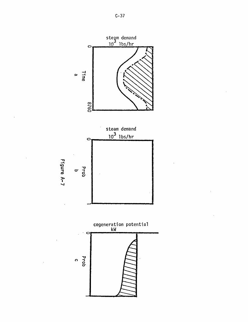
C-37

steam

103

i demand

lbs/hr

cogeneration potentialkW

-1a.

3()

'OC -

O1

-emIl

OCT

Jm i lliiD iiIYY i|MI iYYII

--v -- r

C-38

this system, with the shaded area being that due to condensing steam.

Generation of electricity through the use of a condenser would have a

higher fuel cost since no useful heat will be recovered outside the

turbine. However, this additional cost will be offset by the increased

utilization of the boiler and the turbo-generator. The investment with

the highest present value will depend upon the relative prices of capital

and energy. For a rigorous derivation of this trade-off, see Helliwell

and Margolick (1980).

Gas Turbine Combined Cycle

The gas turbine technology is depicted in Figure Alb. It utilizes

the expansion of gases released by combusting fuel to drive a turbine.

The gas exhausting from the turbine is then channelled through a

waste-heat boiler in which steam is raised. This steam can be delivered

to the process site through a topping turbine (not shown in the diagram)

or a pressure reducing valve. Again, flexibility in the ratio of

electricity to steam production can be maintained through the use of

condensors.

The possible steam demand profiles and cumulative distribution

profiles are portrayed in Figure A8a. Three profiles are shown. The

lower solid line is the demand for process steam. That steam is provided

from the exhaust gases which first produces the electricity. The dashed

line indicates the additional steam demand for electricity production by

steam topping cogeneration. The topping generation strategy implied by

this steam demand profile is one in which the topping turbine is utilized

at full capacity at all times. Additional capital costs to provide this

steam would be a larger combustor and a larger gas turbine. The higher

steam demand

103 Ibs/hr

-4_, a

cogeneration potentialCo kW

OC)4

a0 I0 1

C-40

solid line is a possible profile to provide added steam to be put through

a condenser. Again, the advantage of being able to run steam through a

condensor would be increased utilization of both the gas turbo-generator

and the steam-topping turbo-generator.

The electricity generation load duration curve is found in Figure

8b. The lower solid line is, of course, the electricity production from

the gas turbine. The height between the lower solid line and the dotted

line represents the additional capacity generation that results from

adding a topping turbine. There are two components to this additional

power, the first being that which arises from the topping turbine. The

second component arises from the extra steam that will be required to

make up for heat lost in the topping turbine. That heat will have to be

raised in the fuel combustor, the gases from which will be passed through

a gas turbine larger than the one indicated by the lower solid line. A

large waste-heat recovery boiler would also be required.

A cogenerating strategy does not have to include full use of the

topping turbines. The gas turbine and waste-heat recovery boiler could

be sized just large enough to meet peak process steam requirements with

the topping turbine only large enough to generate electricity from excess

steam. (This is a strategy similar to that described for the situation

in Figure A4.)

The capital costs of these gas turbine cogeneration options are

slightly more complicated to assess forthe joint products than the simple

topping cycle. The smallest system possible results in an investment in

a gas turbine and a waste heat recovery boiler. An additional investment

can be made in a steam topping turbine up to a size large enough to

utilize excess process steam requirements. Topping capacity larger than

IIIMI ll hI I M

C-41

that will require further investments in a larger gas turbine and a

larger waste heat recovery boiler. The thermal efficiency of the

gas-turbine-boiler system can be improved with a balancing condensor to

dampen any remaining fluctuations in the steam requirements.

C-42

Carhart, S. et al. (1979) "The Least Cost Energy Strategy, TechnicalAppendix," Carnegie Mellon University Press.

Cox, A.J. (1981) "The Economics and Regulation of Distributed PowerSystems in the Utility Grid: Photovoltaics," invited paper to theEastern Economics Association meetings, Philadelphia. Available asEnergy Laboratory Working Paper No. MIT-EL 81-014WP.

Cox, A.J. and J.F. Helliwell (1980) "Economic Modeling of Energy Supplyfrom Burning Wood Wastes at British Columbia Pulp and Paper Mills"Resources Paper No. 21, Programme in Natural Resource Economics,University of British Columbia and in W.T. Ziemba et al. (eds),Energy Policy Modelling: U.S. and Canadian Experiences, Vol. 1(Hungham, Mass: 1Martinus Nijhoft), pp. 159-1/4.

Department of Energy (1979) "Industrial Sector Technology Use Model(ISTL1,4): Industrial Energy Use in the United States, 1974-2000."Final report. Vols 1-4. DOE/FE/2344-1.

Dow Chemical Company, Environmental Research Institute of Michigan,Townsend-Greenspan and Company and Cravath, Swaine and Moore (1975)"Energy Industrial Center Study" NTIS No. PB-243-824.

Finger, S (1981) "Integration of Decentralized Generators with theElectric Power Grid." MIT Energy Laboratory Report No. MIT-EL 81-011.

Helliwell, J.F. and A.J. Cox (1978) "Simulation Analysis of EnergyProduction in the B.C. Pulp and Paper Industry' MIT Energy LaboratoryWorking Paper No. MIT-EL 79-009WP.

Helliwell, J.F. and A.J. Cox (1979) "Electricity Pricing and ElectricitySupply, The Influence of Utility Pricing on Electricity Production byPulp and Paper Mills" Resources and Energy Vol 2, pp. 51-74.

Helliwell, J.F. and M. Margolick (1980) "Sore Hard Economics of SoftEnergy: Optimal Electricity Generation in Pulp and Paper Mills withSeasonal Steam Requirements" Resources Paper No. 56, Programme inNatural Resource Economics, University of British Columbia.

Joskow P. and D. Jones (19b1) "The Simple Economics of IndustrialCogeneration" Studies in Energy and the American Economy, MIT EnergyLaboratory Working Paper MIT-EL 81-0 WP.

Joyce, J. (1978) "Energy Conservation Through Industrial Cogeneration"Department of Energy.

Lee, S.T. and Z.A. Yamayee (1980) "Load-Following and Spinning ReservePenalties for Intennrmittent Generation," paper presented at IEEE PESSummer Meeting, Minneapolis, MN.

Olson, D. and H. Kalkstein (1980) "Issues in Cogeneration" Prepared forEnergy Productivity Center, Mellon Institute by Energy andEnvironmental Analysis, Inc., Arlington, Virginia.

C-43

Pickel, F.H. (1978), "Cogeneration in the U.S.: An Economic andTechnical Analysis" Masters Thesis, Department of Civil Engineering,M.I.T.

Pickel, F.H. (forthcoming), "Cogeneration and Utility Planning" MITEnergy Laboratory Technical Report.

Thermo-Electron Corp. (1976) "A Study of Inplant Electric PowerGeneration in the Chemical, Petroleum Refining and Paper and PulpIndustries," prepared for Federal Energy Administration, Contract No.C0-04-50024-00.

Tabors, R., S. Finger and A.J. Cox (1981) "Economic Operation ofDistributed Power Systems Within an Electric Utility" Transactions ofIEEE Power Apparatus and Systems, forthcoming.

Whitman, Requardt and Assoc. (1980) "Handy-Whitman Index of Public UtilityConstruction Costs, Baltimore, MD.

I__ _~_ II YIIYIIII i ii

Massachusetts Institute of Technology

Energy Laboratory

Energy Model Analysis Program

Appendix D

An Analysis of 'Least-Cost' Methodoloy

Michael Manove*

June 1981

*Professor of Economics, Boston University

TABLE OF CONTENTS

1. Is the "Least-Cost Energy Strategy" the Best Strategy?

1.1 General Setting

1.2 Our Modelling Framework

1.3 The Least-Cost Strategy of Producing Energy Services

1.4 The Production of Energy Services with Fixed Capacity

1.5 The Production of Energy Services with Fixed Capacity

Utilization

1.6 The Production of Energy Services with Variable Capacity

Utilization

1.7 Conclusion

2. The Formulation of the Least-Cost Concept

2.1 Which Resource Expenditures Are Counted as Costs?

2.1.1 Money Expenditures vs. Resource Expenditures

2.1.2 Point of View

2.1.3 Capital Goods

2.1.4 Implementation of the Energy Strategy

2.1.5 Diminution of Benefits

2.1.6 Conclusion

2.2 At What Prices Should Expended Resources Be Evaluated?

2.2.1 Resources Traded in Competitive Markets

2.2.2 Regulated Markets

2.2.3 Resources with Strategy-Dependent Prices

2.2.4 Future Costs

2.3 What Variables are Endogenous to the Cost-Minimization

Process?

2.3.1 Capital Stock by Technology Type

2.3.2 Capacity-Utilization Rates of Energy Consuming

Equipment

2.3.3 Efficiency of Energy-Consuming Equipment

2.3.4 Energy Supplies and Prices by Source

2.3.5 Innovation

2.3.6 Limitations of the Least-Cost Methodology

2.4 What Constraints are Used in Conjunction with the

Least-Cost Objective Function?

2.4.1 Simulation of Base-Year Data

2.4.2 The Economic and Technological Environment

3. Conclusions

D-1

Appendix D

An Analysis of 'Least-Cost' Methodology

by

Michael Manove

Minimizing energy costs seems, on a superficial level, to be a

worthwhile objective of energy policy. It has more appeal than various

all-or-nothing alternatives such as a strategy of energy self-

sufficiency. The Carnegie-Mellon Energy Productivity Center (EPC)

describes the least-cost idea with great enthusiasm:

The nation has been on an unproductive course; it has looked atenergy as a diminishing domestic commodity instead of a service whichcould be provided by many competing sources. We have been developinga least-cost strategy which, we believe, could unleash newcompetiitivforces, multiply consumer choices, force down the realcost of energy services over the long run, cut the demand for energysupplies, and make a substantial contribution to the nation'seconomic health. [Emphasis added.]

Unfortunately, as a bit of thought will reveal, the least-cost-

energy strategy is generally not optimal; nor is it easily defined. In

this Appendix, I will examine least-cost methodology with regard to its-

limitations and its use within these limitations.

D-2

1. Is the "Least-Cost Energy Strategy" the Best Strategy?

Least-cost energy strategies are generally not the best strategies,

for two different reasons. First, benefits are not explicitly considered

in the selection of least-cost energy strategies; only costs are

recognized. Second, it may not be reasonable to minimize energy costs

alone, for energy costs are often linked to other costs of production. I

will discuss the first of these problems here.

When a consumer goes to the store to buy an item, he often does not

pursue a least-cost strategy. Taken literally, the least-cost strategy

would require the consumer to buy the cheapest brand. But a consumer is

not interested in cost alone; rather, he is interested in net benefits,

the surplus of bentfits over cost. Therefore, consumers are willing to

buy expensive brands provided that the added cost is justified by the

increased quality of the product.

The concept of a least-cost strategy is meaningful only when some

details concerning the output (or benefits) produced by that strategy

have been specified in advance. "Least-cost for what?" we must ask. If

desired benefits can be specified in advance, then the search for the

least-cost strategy is a useful one. In most situations, however,

consumers are as free to determine the level of benefits as they are to

determine cost. In such cases, the benefits and costs of each

alternative strategy must be evaluated simultaneously.

D-3

Consider, for example, a consumer who is shopping for an automobile.

The consumer is free to make his/her decision on the basis of fuel

efficiency, but is also free ;o decide on the size of the car and amount

of driving. The values that a rational consumer assigns to each of these

variables are interrelated and all will depend on the price of gasoline.

Normally, it would not be rational for a consumer to take the amount of

his driving and the size of his car as fixed and to consider the price of

gasoline only in choosing the appropriate level of fuel efficiency. Yet

the design of a least-cost study postulates exactly that: the quantity of

energy services to be produced and the productive capacity of the

equipment are both specified exogenously; only the efficiency of

energy-service production can be varied.

The least-cost strategy identified in this way can markedly deviate

from the optimal (net-benefit-maximizing) strategy. In order to obtain a

quantitative measure of the nature and degree of this deviation, I shall

employ several elementary analytical models of the production of energy

services. The models I use here were inspired by the more complex and

general models presented by McFadden [2.

1.1 General Setting

The general setting for all of the models presented here is the

same. Some energy service (space-heating, cooling, industrial steam,

transportation) is to be produced by some sort of equipment (furnace,

boiler, air conditioner, automobile) that uses some form of energy input

or fuel. Each strategy of energy-service production is described by

D-4

three variables: the level of energy-service output, the productive

capacity of the equipment and the energy efficiency of the equipment.

These three variables imply values for two other important variables:

the capacity utilization rate and total use of energy inputs or fuel.

The models differ from one another in their designation of which of these

variables are fixed in advance, and which may be set by the consumer or

pol icymaker.

Our first model will represent the selection of the least-cost energy

strategy: the least-cost level of energy efficiency is chosen for a given

output of energy services and equipment capacity. The second model will

represent the selection of the maximum-net-benefits strategy when both

the level of energy services and the energy efficiency of the equipment

can be varied. The third model represents the selection of the

maximum-net-benefits strategy when energy services, equipment capacity

and equipment efficiency can all vary, but where the capacity utilization

rate is fixed. Finally, we shall construct a model of the selection of

the maximum-net-benefits strategy when energy service, equipment capacity

and equipment efficiency can all be varied independently of one another.

The properties of the strategy selected by our representation of the

least-cost model will be compared with those of strategies selected as

optimal by our three net-benefits maximizing models. In this way, we

shall reach some conclusions about the type and degree of distortion

inherent in the least-cost model output because of its restrictive

assumptions.

It is important for the reader to keep in mind that all models

contain simplifying assumptions and that their outputs necessarily

D-5

deviate from reality. These simplifications cannot and ought not be

avoided if the model is to have significant explanatory and predictive

value. In fact, most policy model failures occur because of models that

are cluttered with complex, poorly represented and poorly understood

detailed depictions of the real world. Many models would be greatly

improved if they were cast at a simpler, more highly abstract level.

Thus, we are not objecting to the fact that a least-cost study contains

simplifying assumptions; rather, we are asking when the particular

simplifications made are the appropriate ones for the purposes to which

the study is to be applied.

1.2 Our Modelling Framework

The fundamental policy variables of our models are the level of

energy services, X, the capacity of the service-producing equipment, K,

and the equipment energy/service ratio (ESR), denoted by H. The variable

H is defined by the identity

(1) H = E/X

where E is the total quantity of energy used as an input to the

productive process. Thus the reciprocal of H is a measure of energy

efficiency.

The capacity utilization rate, U, is defined by the identity

(2) U = X/K

Wilk-' -'- ' --- ' -~-- ----- '-

D-6

When cost is the same, consumers prefer lower utilization rates to higher

ones, because lower rates afford the consumer more flexibility in the

production of energy services.

In all of our models, equipment costs will be assumed proportional to

equipment capacity. This is because we are trying to depict the

production of energy services in the aggregate. Equipment capacity is

visualized as being determined by the number of units of equipment

available rather than by the size of each unit. The cost per unit of

equipment is denoted by the function C(H). We assume that lower ESR

values (greater efficiency) are more costly to achieve than higher ESR

values (lesser efficiency), and that there is increasing marginal cost of

increasing efficiency. Thus C'<O and C">O.

The price of energy inputs or fuel is denoted by P. In the models

below, we shall examine how the value of P effects the optimal value of

the other variables.

1.3 The Least-Cost Strategy of Producing Energy Services

Let the output of energy services, X, be fixed and, for simplicity,

assume that the equipment capacity, K, is fixed at K = 1. Then, total

cost of producing energy services is given by

(3) T = C(H) + PXH

D-7

Note that HX is the quantity of fuel consumed in the production process,

so that PHX is the total cost of fuel consumed. The cost-minimizing

strategy is determined by the energy/service ratio, H, that minimizes T.

This first-order condition for the optimal value of H is given by

(4) -C'(H) = P

Suppose, now that C(H) is defined by

(5) C(H) = c + mH-"

for v > 1. The parameter co represents the base price of a unit of

capacity, and the parameter p represents the elasticity of additional

equipment cost with respect to energy efficiency.

Differentiating (5), we have

(6) C'(H) = -mvH - v- 1

Subtituting (6) into (4) yields

(7) log(mp/X) - (p+l)h = p

where h and p are the respective logarithms of H and P. By

differentiating (7) with respect to p and solving for h' we obtain

1(8) h' 1 + 4

Note that h' is the elasticity of the least-cost H with respect to

the price of fuel, P. Thus -h' is the elasticity of energy efficiency of

I MMM WAWMMIM

D-8

the least-cost production strategy with respect to the price of fuel.

If, for example, v = 1, then a doubling of the price of fuel will cause

the energy efficiency of the least-cost strategy to increase by about 40

percent. We will show that this figure substantially exceeds the

analogous figures obtained from some of the maximum-net-benefits models.

1.4 The Production of Energy Services with Fixed Capacity

In this model, we shall assume K is exogenously specified at K = 1,

and allow both X and H to vary. As an example, think of a consumer that

must have a two-ton truck in order to haul large fixtures. The consumer

can select the efficiency of his truck and can determine the extent of

its use. The consumer derives benefits (revenue) from the services

provided by the truck, but must pay both capital costs and mileage costs.

Let B(X) denote the benefits to the consumer of the level of service

X. We assume decreasing marginal benefits, i.e. B'>O and B"<0. The net

benefits associated with any values of X and H is the difference between

the benefits of the energy service and its costs. This is given by the

function i(X,H) where

(9) w(X,H) = B(X) - C(H) - PHX

The maximum-net-benefits strategy is given by the solution of the

following problem:

max 7(X,H)X,H

D-9

The first-order conditions for the maximum-net-benefits strategy are

given by (4), repeated here,

(4) -C'(H) _ p

and by

(10) B'(X)

A second-order condition sufficient to guarantee that the solutions of

(4) and (10) describe a maximum-net-benefits strategy is given by

(11) -B"(X)C"(H) > P2

We now find the solutions of (4) and (10) for particular

specifications of benefits and cost functions. Let B(X) be defined by

(12) B(X) =- X( )/

for a > 0, a / 1. This benefits function was chosen because it implies a

demand function for X with a constant own-price elasticity of -a.

Let C(H) be given by (5), as before.

Differentiating (12), we have

(13) B'(X) = bX- 1 / a

Let x, h and p denote log X, log H and log P, respectively. Substituting

(6) and (13) into (4) and (10) and taking logarithms yields the

- 111111 11111401

D-10

logarithmic form of the first-order conditions for the

maximum-net-benefits strategy:

(14) log(b) -1x - h = p

and

(15) log(mv) - (p+l)h - x = p

Equation (15) is equivalent to (7), but in (15) X is not a constant. The

second-order condition (11) will hold if and only if

(16) 1 + - a > 0

Therefore, a maximum-net-benefits strategy will exist at positive values

of X and H if and only if (16) is true.

Equations (14) and (15) implicitly define x and h as functions of p.

Differentiating (14) and (15) with respect to p and solving for x' and

h', we have

(17) x' = - a

and

(18) h' = 1 - a

The logarithmic derivatives x' and h' are the elasticities of X and H

with respect to P, the price of energy inputs. Because the demand for

energy is given by E = XH the own-price elasticity of the demand for

D-1 1

energy is given by e' = x'+h', so that

(19) e' = - + ai- a +

Condition (16) implies that both x' and e' will be negative. But, we can

see from (18) that h' will be positive if a > 1. Thus, as Khazzoom[1]

and McFadden [2] observe, it may be desirable for consumers to decrease

the efficiency of their equipment when the price of onergy rises' In our

model, this somewhat surprising behavior will occur w\henever consumer

demand for energy services is price-elastic. The intuitive reason for

this phenomenon is easy to understand. A consumer with an elastic demand

for energy services responds to an increase in energy price with a very

large decrease in the use of his equipment. Therefore, he no longer

needs to have equipment that is as energy efficient. Of course, his

total energy use will still decline.

By comparing (18) to (8), we can estimate the overstatement of

optimal equipment efficiency associated with least-cost analysis when

demand for services can vary. If the true price-elasticity of demand for

energy services is zero, then (18) becomes the same as (8) so that cost

minimization will identify the appropriate energy strategy. But if the

price-elasticity of the demand for energy services is non-zero, cost

minimization yields an exaggerated result. Recall that for v = 1 cost

minimization (8) yields h' = -.5, so that optimal efficiency increases

by about 40 percent when the price of energy inputs doubles. But if the

elasticity of demand for energy services is .5, then the

maximum-net-benefits strategy described by (18) calls for an efficiency

-^I'--IIIIYIYIY

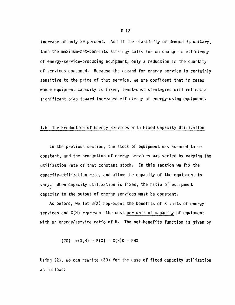
D-12

increase of only 29 percent. And if the elasticity of demand is unitary,

then the maximum-net-benefits strategy calls for no change in efficiency

of energy-service-producing equipment, only a reduction in the quantity

of services consumed. Because the demand for energy service is certainly

sensitive to the price of that service, we are confident that in cases

where equipment capacity is fixed, least-cost strategies will reflect a

significant bias toward increased efficiency of energy-using equipment.

1.5 The Production of Energy Services with Fixed Capacity Utilization

In the previous section, the stock of equipment was assumed to be

constant, and the production of energy services was varied by varying the

utilization rate of that constant stock. In this section we fix the

capacity-utilization rate, and allow the capacity of the equipment to

vary. When capacity utilization is fixed, the ratio of equipment

capacity to the output of energy services must be constant.

As before, we let B(X) represent the benefits of X inits of energy

services and C(H) represent the cost per unit of capacity of equipment

with an energy/service ratio of H. The net-benefits function is given by

(20) w(X,H) = B(X) - C(H)K - PHX

Using (2), we can rewrite (20) for the case of fixed capacity utilization

as follows:

D-13

1(21) I(X,H) = B(X) - UC(H)X - PHX

where U is the constant capacity-utilization rate. The first-order

conditions for the maximization of (21) are given by

1(22) B'(X) = -C(H) - PHU

and

(23) C'(H)X = UPX

If X is positive, (23) reduces to

(24) C'(H) = UP

Let us now specify the function C(H) by equation (5), so that C'(H) is

given by (6). Substituting (6) into (24) and taking the logarithm of

each term in the resulting equation, we get

(25) log(mv/U) - (p+l)h = p

where h and p are the logarithms of H and P, respectively.

Differentiating (22) with respect to p and solving for h' yields

1(26) h' = - 1

- TP~

But (26) is identical to (8). This means that if the

--- ~ ^ IIIIIIIII l 6111111ii

D-14

capacity-utilization rate is fixed, as we have assumed for this model,

the least-cost strategy is a good approximation for the

maximum-net-benefits strategy with regard to the energy-efficiency of

equipment. This is true even if the demand for energy services is price

elastic. Of course, because least-cost analysis contains no counterpart

of equation (22), it cannot tell us anything about the output of energy

services.

1.6 The Production of Energy Services with Variable Capacity Utilization

In this section, we allow both productive capacity (for producing

energy services) and capacity utilization to vary. In other words, the

level of the production of energy services and the capacity to produce

those services can vary independently. It is important to understand

that the presence of productive capacity creates benefits even when it is

not being used. This is because excess capacity allows increased

flexibility in the rate that services are created. Because of the need

for flexibility, people are often willing to pay for capacity in excess

of minimum production requirements. Therefore, in this section, we will

consider the benefits of energy services to be an increasing function

both of the level of services and the amount of capacity available to

produce those services. Benefits will be denoted by B(X,K). This will

make our model a bit more complicated than the previous models in which

benefits were functions only of the level of services, X.

In this model, net benefits are given by

D-15

(27) ir(X,K,H) = B(X,K) - C(H)K - PHX

First-order conditions for maximizing w are given by

(28) B= PH

aXB(29) aB = C(H)ar

and

(30) -C'(H)K = PX

In order to present one e>ample of how X, K and H might depend on the

price of energy, P, we will specify the following form for B(X,K):

(31) B(X,K) = bX'YK Y,B > 0, Y,8 < 1

This particular functional fbrm (Cobb-Douglas) is a plausible, but by no

means general, benefits function. The value y+o is the elasticity of

benefits with respect the the level of energy services when the capacity-

utilization rate is held constant.

We specify the cost-of-efficiency function, C(H), by (5), as before.

Differentiating (31) and (5), substituting the results into (28), (29)

and (30) and taking logarithms yields

log(by) + (y-l)x + sk - h

log(bs/m) + yx + (s-1)k

log(m) - x + k - (i+l)h

= p

- log(C(H)) = 0

p

(32)

(33)

(34)

II . .. I i aIllIII ,, hI

D-16

Differentiating these equations with resect to p yields the equations:

(35) (y-1)x' + sk' - h' = 1

(36) yX' + (s-1)k' + PSh' = 0

(37) -x' + k' - (p+l)h' = 1

where S is the ratio of efficiency costs to total capacity costs given by

(38) S mH'c + mH-

These equations can be solved for x', k' and h', the elasticities of X, K

and H with respect to P. The solutions are:

1-8

(39) x' = -X 1 - (+s)

(40) k' = -S"- (Y+B)

and

(41) h' = 0

Equation (41) implies that for the Cobb-Douglas benefits function, the

optimal energy efficiency of productive equipment is independent of the

price of energy. How can this be so From (2) we know that u', the

elasticity of the utilization rate with respect to the price of energy,

is given by u' = x' - k', so that by (39) and (40), u' = -1. Thus, as

the price of energy increases, productive equipment is used less

D-17

intensively. Although increased energy prices tends to increase optimal

efficiency, the accompanying reduction in utilization rate negates that

optimal-efficiency increase.

Suppose, for example, that y = -1/4 and s = 3/4. From (39) and

(40), we have x' = -1/2 and k' = 1/2. Therefore,.if fuel prices double,

the demand for energy services will fall by about 30 percent. The

capacity of the equipment, however, will increase by about 40 percent.

This increase comes about because consumers find equipment has become

less expensive as compared with the cost of energy services. Thus, for

example, after an increase in the price of gasoline, consumers may choose

to own more cars on the average, even if they decrease their total

mileage. Each car would be used significantly less, so that consumer

willingness to pay for increased fuel efficiency would be less than it

otherwise might be.

This model brings out a very important aspect of the production of

energy services. Increases in energy prices tend to decrease optimal

equipment utilization, and decreased utilization decreases optimal

efficiency. Thus, optimal efficiency is bound to be less than would be

indicated by least-cost analysis, in which productive capacity and the

rate of capacity utilization are both held fixed. The distortion

associated with least-cost analysis might be less (or more) dramatic than

the distortion that appears with the Cobb-Douglas benefits function, but

some distortion will be present. This type of distortion is independent

of the elasticity of demand for the energy service, and it will exist

even if that demand is perfectly inelastic.

D-18

1.7 Conclusion

In Section 5, we suggested that least-cost analysis tends to be a

good approximation of maximum-net-benefits analysis whenever

capacity-utilization rates of service-producing equipment are fixed. But

while fixed capacity-utilization rates may be a realistic discription of

certain sectors of the economy, it is unreasonable to assume that

capacity utilization rates for the economy as a whole will remain

unchanged when energy prices are drastically increased.

We must conclude, therefore, that a least-cost energy strategy may

strongly overstate desired increases in efficiency. This can occur for

two different reasons. First, there are miny situations in which the

capacity of equipment must remain relatively fixed, despite changes in

the price of fuel. If, in such cases, the demand for energy services is

price sensitive, then increased fuel prices will cause capacity-

utilization rates to fall and least-cost analysis will overstate optimal

efficiency increases. This tendency was demonstrated in Section 1.3.

Second, when the level of productive capacity and the quantity of energy

services can vary independently, consumers (or producers) will tend to

substitute additional capacity (and flexibility) for the energy service

itself. This lowers utilization rates and optimal efficiency. This

tendency was demonstrated in Section 1.6.

It is a general principle of economics that the existence of

substitutes in production and consumption tends to reduce the impact of

external economic shocks. The methodology of least-cost analysis allows

D-19

increased efficiency in the production of energy services to substitute

for energy-inputs or fuels, as energy prices rise. However, that

methodology excludes the possibility of substituting increased

flexibility in the production of energy services for some portion of

those services. Least-cost methodology also excludes the possibility of

substituting the consumption of non-energy services for the the

consumption of energy services. BIecause of these characteristics,

least-cost methodogy will tend to overstate both the importance of

increases in energy efficiency and the overall impact of high energy

prices on the economy as a whole. The general perspective created by

least-cost analysis may be seriously biased.

2. The Formulation of the Least-Cost Concept

Having already raised some questions about the desirability of the

least-cost approach, I would like to consider the meaning of the terms

"cost" and "least-cost," and discuss the different ways in which the

concept of least cost can be formulated. The task of adding up the costs

of providing energy services to the entire nation is extremely broad and

varied. In pursuit of this endeavor, even the most detached analyst will

be forced to make a long series of decisions entailing value judgments

and predictions. These decisions will constitute an implicit definition

of what the analyst means by the cost of a strategy and will ultimately

affect choice of which strategy is the least-cost strategy.

Here are some examples of decisions that must be made in computing

the cost of a national energy strategy: Should payments for

II- - - M,

AIMIMM

D-20

already-existing capital goods be counted as costs? What value should be

placed on environmental quality? Should the actual price of natural gas

be used to evaluate the cost of gas? Or, should the analyst use some

estimate of the price of gas that would prevail in the absence of

regulation? What are appropriate minimum ambient temperatures.for

various categories of buildings? If a strategy includes governmental

regulations, should costs be computed on the assumption of complete

compliance with those regulations? If not, how should the costs of

cheating be evaluated? Will a particular strategy induce innovation and

market penetration of new, more efficient technologies? Should the

quantity of available oil be constrained to equal known reserves? Or

should the discovery of new deposits be assumed?

It should be obvious, I think, that there are no clear-cut right or

wrong answers to these questions. Many of the answers ought to turn on

the purpose of the cost calculations. But one point is clear: The

identification and description of the least-cost strategy will be of

little value unless the analyst diligently communicates his answers to

all of these questions and many others. In fact, any depiction of a

least-cost strategy without careful documentation of these decisions may

prove to be seriously misleading.

Each of the cost-defining decisions tends to answer one of the

following four general questions: Which resource expenditures are

counted as costs? At what prices are expended resources evaluated? What

variables are endogenous to the cost-minimization process? What

constraints are used in conjunction with the least-cost objective

function? One of the sections below is devoted to each of these general

_ _I~^_)__ ___~ I

D-21

questions.

2.1 Which Resource Expenditures Are Counted as Costs?

Answering this question requires a number of careful value

judgments. Below, I discuss some general points that arise in connection

with costing out all resources, and then I discuss costing-out specific

resources.

2.1.1 Money Expenditures vs. Resource Expenditures

It is important to consider as costs the real use or expenditure of

scarce economic resources rather than money payments. Sometimes the two

go together, but sometimes they do not. For example, federal, state and

local taxes are money costs that do not, in themselves, involve the

expenditure of scarce economic resources. Thus, taxes normally should

not be counted as an economic cost. However, when a specific energy

strategy requires the government to provide a certain service, the value

of that service should be counted as a cost.

The degradation of the environment is an example of a resource

expenditure usually not associated with a money payment. It is important

to count all such costs, even though it may be difficult to assign a

value to them.

.... . . ... .... llllr II oi , l ll i i ll li iIll II ll iI llNI 1 guI IuuYYIuInuurnnI ImuIuuglYI M I IYII .I

D-22

2.1.2 Point of View

This brings us to a closely related and equally general point: From

whose point of view are costs defined? From the point of view of

corporate stockholders, the corporate income tax is a cost, because it

gives the government, an 'outsider,' a claim on the real resources owned

by those stockholders. But from the point of view of the nation as a

whole, the corporate income tax is not a cost. It is simply a transfer

of resources from one group of citizens to another; both groups are

'insiders.' No resources are actually expended in that transfer.

We are frequently concerned about costs from the national point of

view. Thus, for example, all of the funds paid to foreign governments

for oil are considered to be costs. This makes sense because those funds

give foreigners (outsiders) a claim on our own real resources. It should

be understood, however, that it would be perfectly valid for an analyst

to be concerned with costs from the point of view, say, of all of

humanity. In that case, the profits paid to an OPEC member by virtue of

OPEC's monopoly power would be considered a simple transfer of resources

from one inside group to another, and not a true expenditure of

resources. Only the "competitive" value of oil would be counted as a

cost, for only that part of the money payment represents the value of the

oil in its best alternative use.

When the analyst determines the point of view, she is making a value

judgment that cannt be declared 'right' or 'wrong.' But those of us who

form the audience For the analysis are entitled to know whose point of

view was adopted.

D-23

2.1.3 Capital Goods

Should the (levelized) cost of existing in-place capital goods be

included in the cost of an energy strategy? The answer to this question

depends on the purpose of the least-cost analysis.

Suppose, for a moment, that the analysis was motivated by the

following question: "How much would we have saved if we had had the

foresight to invest in efficient capital equipment rather than in the

inefficient equipment we now use?" This is a question of historical

interest. It is addressed to what we should have or might have done, not

to what we ought to do at the current time. The motivating question

implicitly requires that we view the world from the standpoint of the

time before current investment decisions were made. Thus, in trying to

answer this motivating question, we must put existing capital goods on

the same footing as alternative capital goods. Therefore, the cost of

both existing and alternative capital goods should be included in our

calculations.

Suppose, however, that we are attempting to solve the very practical

planning problem: "In what type of equipment should we now invest?" In

asking this question, we are looking forwards, not backwards. We must

view the installation of existing equipment as an irreversible event. If

existing equipment has no use other than to produce energy services, then

there are no economic costs (lost opportunities) entailed in using it for

that purpose. Therefore, in this case, capital charges for existing

equipment should be excluded from our calculations. Capital charges for

--- '-loIYIImIlI ilmiliii Al

D-24

new equipment, however, should be fully included.

The analyst's Jecision to include or exclude capital charges on

existing equipment is a crucial one. It should be documented and

carefully justified.

2.1.4 Implementation of the Energy Strategy

We now turn our discussion to issues that relate to the social

organization of energy production. These social issues frequently entail

substantial resour:e expenditures.

Consider an energy-production strategy that requires a well-insulated

housing stock. For that strategy to be implemented, homeowners must be

informed that insulation is advantageous and induced to install it in

their homes. I.f the economic benefits of insulation do not accrue

directly to the homeowners, if the homeowners do not perceive those

benefits, or if the homeowners are irrational, then regulation and

enforcement may be necessary to implement an insulation program.

Providing homeowners with information on 'nsulation and its economic

effects may be costly. The regulatory process can also be extremely

costly. Vast resource expenditures may be required to enforce

regulations. Should these costs be included in the cost of the

associated energy strategy?

Or consider the following closely related question. Suppose that a

particular strategy calls for a large number of nuclear power plants.

These plants are highly unpopular among some segments of the population,

and their construction might make those people very unhappy indeed.

________________________________ . nImY IhIUY hII IIIIIIIINIEIIJ II i m

D-25

Should such "psychological" costs be included in the analyst's cost

calculations? Suppose that the construction of nuclear power plants

would likely induce widespread social unrest? Should the cost of such

unrest be tabulated and included in the cost of the associated strategy?

The appropriate answers to these questions depend on the identity of

the policymakers for whom the least-cost analysis is intended. If one

wants to convince nuclear opponents that nuclear power is desirable

because it is inexpensive, it does not make sense to include the

psychological state of those nuclear opponents as a cost of nuclear

power. But if the analysis is being conducted on behalf of'a politician

who is concerned with popular sentiments as well as with dollar and

cents, it may make perfect sense to convert sentiments to dollar-costs.

2.1.5 Diminution of Benefits

The least-cost methodology explicitly excludes consideration of the

benefits of energy service, a fact I have discussed at some length. In

principle, energy services are specified in advance, and all strategies

considered provide the same energy service. In fact, however, no two

energy strategies provide exactly the same energy services. For example,

improvements in the thermal shell of buildings may degrade ventilation to

some extent, causing benefits of space heating to be slightly

diminished. In order to make different energy strategies comparable,

such diminutions of benefits can and should be treated as costs of the

strategy with which they are associated. Any increases in benefits

I lMilIMMUM

D-26

should be subtracted from strategy costs.

Very often, energy-efficient equipment is less convenient than

energy inefficient equipment. Efficient automobiles are often

characterized by cramped interiors, sluggish acceleration, high noise

levels and manual transmissions. Such inconveniences should be charged

off as added costs of efficiency if the analysis is to avoid a

pro-efficiency bias.

Of course, translation of inconveniences to costs requires numerous

value judgments. Often, these judgments can be facilitated by data

descriptive of consumer willingness to pay for added conveniences.

2.1.6 Conclusion

There are no simple answers to the question: "Which resource

expenditures should be counted as costs?" Many decisions in this area

require value judgments by the analyst. Many decisions depend on the

point of view of the analysis. It is essential, therefore, that these

decisions be well-documented and explained.

2.2 At What Prices Should Expended Resources Be Evaluated?

The evaluation of expended resources is a difficult process requiring

good judgment and forecasting ability. When a resource is bought and

sold in a competitive market, the actual price tends to reflect true

economic scarcity. Therefore, competitive prices are normally a good

D-27

index of current resource value. Unfortunately, competitive prices are

often unavailable to the analyst. This may be because a resource is not

traded in a competitive market, or it may be because the analyst cannot

secure the relevant market data. Often, the analyst needs to know the

future value of a resource, and it may be difficult to forecast such

values even when current values are known. There is no single "right"

way to evaluate resources, but there are many wrong ways to do it. I

will discuss a number of them.

2.2.1 Resources Traded in Competitive Markets

When a resource is traded in a competitive market, the competitive

price forms a good starting point for resource evaluation. But even in

this simplest case, difficulties can arise. As an example, consider the

case of coal. Coal is one of the few basic energy sources whose supply

is competitive. But coal is not homogeneous; nor is the railroad system

that transports the coal. Since coal supplies differ by quality and by

location, there are a very large number of competitive prices available,

one for each type of coal and for each location in which it is traded.

Furthermore, although the national market for coal tends to be

competitive, some firms may exercise local monopoly power. More

importantly, the market for coal miners is unionized. Consequently, the

wage bill in the coal-mining sector may overstate the true economic costs

of that labor. This would be reflected in the market price for coal, so

that a downward price adjustment might be desirable.

There are other non-competitive factors in coal supply. Some states,

^1 1 1111111111*1

D-28

and the federal government have imposed taxes and royalty charges on coal

production. These fees may affect a sufficiently large proportion of

coal to drive up its market price in some regions.

We can see then, that even competitive prices should be examined to

determine how well they reflect underlying economic scarcity. They may

deviate from scarcity values for a variety of reasons: non-competitive

elements in resource supply and transportation, externalities in resource

production, or because of buyers and sellers who are poorly informed

about market conditions or who have incorrect expectations about the

future. When substantial deviations exist, price adjustments in the

computation of costs may be desirable.

2.2.2 Regulated Markets

Prices in regulated markets rarely have the virtue of reflecting true

economic scarcity. Therefore, it is important to try to estimate the

economic cost of delivering marginal units of the resource involved.

This is an extremely difficult task. For ,atural resources, like gas,

both production and depletion costs must b! consider(!d. And depletion

costs, the value of the resource in its ne.t best alternative use

(possibly in the future), cannot be calculated with conventional

accounting procedures. Some economists have proposed complicated dynamic

optimization techniques to find them, but at this time the state of the

art has not been advanced far.

Both natural gas and electricity fall into the category of resources

whose production and sale are regulated, and there is reason to believe

D-29

that their regulated prices underestimate their economic value. The

analyst must do his/her best to make appropriate price adjustments. The

difficulty of the problem is not a good reason to cost out these

resources at the regulated price.

2.2.3 Resources with Strategy-Dependent Prices

When the production of energy services consumes a large portion of

the available quantity of a resource, the price of that resource may well

depend on the energy strategy implemented. In such cases, estimating the

economic cost of the resource used up by a given strategy, requires

knowledge not only of the price that would prevail given the

implementation of that strategy, but of the entire supply curve for that

resource. This is because of the fact that the a competitive market

price reflects the economic cost of the marginal (last) unit of the

resource delivered; previous units are less costly. If a strategy uses

only a small portion of the supply of a resource, then the value of the

last unit is a good approximation for the value of all units used by that

strategy. Otherwise, each succeeding unit of the resource must be valued

differently. The conventional technique for evaluating the cost of such

a resource is to calculate the area under the supply curve, bound by the

quantity of the resource usage external to the strategy, on the one side,

and total resource usage, including that of the strategy, on the other

side.

A supply curve for a resource is illustrated in Figure I. Suppose

the non-energy sector of the economy uses quantity Qo of the resource,

D-30

while the energy-service sector specified by a given energy strategy uses

quantity Q of that resource. Then the shaded area corresponds to the

economic cost of the resource used up in the given strategy.

As an example, consider an energy strategy specifying extensive

retrofitting of heating systems. Suppose that the retrofitting work

would use a substantial portion of the available labor. time of plumbers

over a period of several years. To calculate the economic cost of the

plumbers' labor, one would determine the supply curve for plumbers, and

calculate the area designated in Figure 1. Notice that the last plumber

used costs quite a bit more than the first plumber used. Because more

and more plumbers are used, each succeeding plumber is withdrawn from

important alternative work.

Figure 1

Price

SupplyCurve

- Economic Costof Resource

Quantity of

QQ+Q ResourceQo 0

D-31

2.2.4 Future Costs

Calculating the cost of an energy strategy projected into the future

requires some form of economic forecasting ability. Good forecasting

techniques can range from educated "guestimation" to sophisticated

econometric forecasting models. In order to obtain some sort of

confidence interval for cost estimates, it is important to conduct

sensitivity studies with respect to all forecasted parameters and data.

Usually, it is useful to present results for several variants of the key

parameters.

If important parameters are highly uncertain, the strategy that is

optimal for the most likely (or expected) outcome of the parameters

generally will not be the optimal strategy. This is because of the need

to "hedge one's bets" in an uncertain world. If key parameters are

unknown, it is often best.to postpone irreversible commitments.

Consider, as an example, the problem of developing a strategy for

long-term investments in electricity generating equipment. If it is

certain that in the future coal-fired boilers will be less expensive to

operate than gas-fired boilers, then coal-fired boilers should be

installed. If the opposite is certain, then gas-fired boilers should be

installed. But it does not follow that a combination of gas-fired and

coal-fired boilers is a good strategy when relative costs are uncertain.

It may be much better to hedge with stop-gap investments in small gas

turbines until more information emerges about future costs.

In short, the kinds of strategies appropriate to a highly uncertain

world are qualitatively different from those suited to a certain world,

_ ___ I~~ ~_ _ _

D-32

whatever the description of that certain world may be. The best strategy

for the best guess about future prices may be a poor strategy indeed. To

find the least-cost strategy in the face of uncertainty, the analyst may

be best advised to use stochastic optimization techniques. Needless to

say, the application of such complicated techniques to large systems of

variables is highly problematical. In any event, an appreciation of the

implications of uncertainty is useful.

2.3 What Variables are Endogenous to the Cost-Minimization Process?

The analyst's answer to this question will determine the scope of the

policy model. The analyst must find a natural boundary for the problem.

All variables outside that boundary are to be specified as parameters in

advance of the analysis or omitted from consideration entirely; the

values of the variables within that boundary will be determined by the

analysis itself. In the design of a policy model for selecting a

minimum-cost energy strategy, there are a number of broad classes of

candidates for endogenous variables. These include important

macroeconomic variables, capital stock by technology type, energy

supplies by source, utilization rates of energy-using capital, innovation

of energy-related technologies, energy prices, and prices of non-energy

resources.

Selecting the endogenous variables for a policy model is an

analytical task requiring substantial creativity. Nevertheless, a few

general common-sense rules may be formulated. Variables that define the

D-33

strategy being sought must be endogenous. With respect to the selection

of a least-cost energy strategy, the capital stock by technology type is

at the heart of any strategy description, and so must be endogenous.

Variables whose values are sensitive to the strategy chosen should also

be endogenous. If a group of variables is highly interdependent, then

either all should be endogenous or else enough of them should be

exogenously specified to determine the rest uniquely. For example, it

would not be logical to make the supply of coal endogenous and the supply

of natural gas exogenous.

If one variable causally determines the value of another, it would

not make sense to have the former endogenous and the latter exogenous.

More generally, causality may run from exogenous variable to endogenous,

from endogenous to endogenous, but not from endogenous to exogenous.

These rules are a rough guide to logical consistency in policy model

design. But the overall blueprint of the model, the decision about what

variables will be at its focus, should depend on the ultimate purpose of

the analysis. Almost every variable explicitly represented in a model

adds to its conceptual difficulty, its cost and its completion time. It

is important to keep this fact in mind during the crucial task of

choosing the level of aggregation for the model. Variables should be

omitted entirely unless they are to the point of the analysis. It

probably would not be a good idea to have a variable representing

academic salaries in a model of energy strategies. Academic salaries are

extraordinarily important, but, in the opinion of most authorities on the

subject, they are not closely related to the energy question. Every

variable included in the analysis should be relevant from a conceptual

D-34

point of view.

I will now proceed to consider some specific classes of variables.

Then I will discuss the limitations of the least-cost methodolgy in this

connection.

2.3.1 Capital Stock by Technology Type

The capital stock of energy-service producing equipment is at the

heart of any energy-strategy model, and must be represented as a decision

variable. The difficult question in this connection is the appropriate

level of detail. In general, it is usually suggested that highly

aggregated representations are preferable until the structure of the

model is well understood and under control.

2.3.2 Capacity-Utilization Rates of Energy Consuming Equipment

As I have explained in a previous section, capacity utilization rate

variables are extremely important aspects of an energy strategy. Along

with fuel prices, they determine the appropriate rate of substitution

between capital costs and energy efficiency. With the cost of obtaining

efficiency given, the higher the energy price and the higher the

utilization rate, the more efficiency is justified.

D-35

2.3.3 Efficiency of Energy-Consuming Equipment

The efficiency variable is at the foundation of any energy strategy.

It may be represented either as a continuous variable, where each level

of efficiency has an associated capital cost, or as a discrete variable,

associated with the technology type of the equipment and the cost of that

equipment.

2.3.4 Energy Supplies and Prices by Source

If the energy strategies under study are U.S. national strategies,

then energy prices and associated supply variables that depend on those

strategies should be endogenous. The domestic supplies and prices of

coal and natural gas are examples. If prices are modelled as exogenous

parameters, there is an implicit assumption that supply is perfectly

elastic at its parametrically given price. This is unrealistic for coal

and gas. If quantities are modelled as exogenous parameters, then there

is an implicit assumption that supply is perfectly inelastic or,

equivalently, that the amount of the resource that can be obtained is

independent of extraction or production costs.

2.3.5 Innovation

In the long run the amount of innovation that occurs in the area of

energy production and consumption will depend partly on the price of

energy inputs and services. Therefore least-cost energy analysis with

long time horizons should make energy innovation an endogenous variable.

0-36

Of course, it is very difficult to make accurate predictions about the

quantity and effect of innovations. The analyst may choose to seek

expert opinion.

2.3.6 Limitations of the Least-Cost Methodology

As I have noted above, least-cost methodology requires that benefits

be exogenous and specified in advance. Therefore, there are several

categories of variables that cannot be endogenous to a least-cost model.

These include demands for energy services and macroeconomic variables.

The prices of energy services will be highly sensitive to the energy

strategy selected. Therefore, if the demand for a particular energy

service is price-elastic, then the quantity of that service demanded

should be, but cannot be, endogenous to the least-cost model. To specify

demand exogenously is to assume that either the price of energy services

will not depend on the energy strategy, or that service demand is price

inelastic. This is unrealistic for most energy services.

Energy is so fundamental to our economy that our overall economic

performance is likely to depend on the energy strategy selected.

Therefore, it would be desirable to endogenize a number of key

macroeconomic variables. But this is incompatible with the least cost

methodology.

The inability of the least-coast methodology to represent the causal

connection between energy strategy, on the one hand, and demand and

macroeconomic performance, on the other, is a serious limitation of that

methodology.

D-37

2.4 What constraints are used in conjunction with the least-cost

objective function?

The least-cost methodology is a methodology of constrained

minimization. The very concept of least-cost has no meaning until

sufficient constraints are specified to define the feasible set of energy

strategies. The audience for a least-cost study will be unable to

interpret its results without clear knowledge of the model constraints.

2.4.1 Simulation of Base-Year Data

At some time during the process of model development, it is important

to have the model constrained sufficiently to simulate actual production

of energy services during the base year for which data is available.

Forcing a model to simulate known data has two benefits. First, the

model is partially validated. A model that cannot correctly simulate

something that has actually happened probably cannot simulate future

events of a similar nature. Second, the set of constraints needed to

simulate the base-year case provides a point of comparison with different

sets of constraints yielding different least-cost strategies. When we

see a strategy with a lower cost than that associated with existing

behavior, it is useful to be able to answer the question, "What

constraints were dropped?"

D-38

2.4.2 The Economic and Technological Environment

Constraints must be used to describe various features of the economic

and technological environment including energy sources, energy conversion

technologies and industrial production technologies. Furthermore, upper

and lower bounds on stocks of certain capital goods must be present in

order to force model conformance with real-world base-year capital

stocks. It would not make much sense to allow the model to make drastic

changes in the stock of structures over a short period, for example.

Constraints must often be added to the model in order to force a measure

of realism on areas of the model that are loosely specified. In models

that do not endogenize innovation and technical change, it may be

desirable to have constraints on rates of technical change and market

penetration of new technologies.

3. Conclusions

The most serious limitation of the least-cost methodology is that it

focuses on costs and cannot take benefits into account. But both costs

and benefits depend on the national energy strategy selected. To specify

a level of benefits or energy services that prevailed during a period of

low energy prices biases the energy strategy that i; chosen towards

increased efficiency in energy consumption.

The least-cost methodology does have the advantige, however, of

D-39

avoiding all of the problems attendant to benefits computation. This is

one argument that can be made in favor of its use. In the context of

selecting a national energy strategy, however, I do not find the argument

convincing. As I have pointed out above, the concept of cost has

critical subjective elements, as does the concept of aenefits. The

decisions of the analyst regarding the evaluation of expended resources

can have a critical impact on cost figures.

The subjective elements in least-cost analysis impose a number of

obligations on the analyst. The analyst must be consistent in approach.

Decisions must be appropriate for the purpose of the analysis. But most

important of all, the analyst must meticulously document an.1 subjective

input and assumptions. Lack of such documentation prevents other parties

interpretion of the results of the analysis in a meaningful way and can

cause those results to be confusing or misleading.

References

l]3 Khazzoom, J. Daniel, "Economic Implication of Mandated EfficiencyStandards for Household Appliances," Journal of EnergyEconomics, October, 1980.

[2] McFadden, Daniel, "An Evaluation of the ORNL Residential Energy-UseModel,." MIT-EL 81-021, Energy Model Analysis Program, MIT EnergyLaboratory, manuscript, 1981.