A Response of High School Teachers to the Adoption of State Economics Standards

Mohammed Khayum, Gregory Valentine, and Daniel Friesner

Abstract This paper addresses the recent adoption of economics standards in the state of Indiana. The analysis is based on responses to a survey instrument that was designed to obtain information about the demographic profile of high school economics teachers, their coverage of the topic areas included in the economics standards, and the critical challenges they face as high school economics teachers. We find that while virtually all teachers in our sample deviate from the standards, the magnitude of the deviation is small, and occurs in a predictable way. Most teachers appear to spend slightly less time on microeconomics (43.2% versus the mandated 50%) and international economics concepts (9.1% versus the mandated 12%) in favor of additional personal finance topics (19% versus 10%). As a result, the standards appear to be moderately successful in achieving its intended goal of creating convergence in content coverage in high school economics curricula.

JEL Code: I21

Key Words: Educational Economics

Introduction

Two evident empirical trends in high school economics education are the higher

proportion of high school students who take an economics course and the substantial increase in

the number of states that have adopted economics standards for inclusion in the high school

curriculum. Between 1961 and 1994, the percent of high school students taking an economics

course rose from 16 percent to 44 percent (Walstad, 1992; Walstad and Rebeck, 2000). The

number of states that have adopted economics standards either voluntarily or as result of

mandates increased from 38 to 48 between 1997 and 2002 (NCEE, 2003). Moreover, between

1982 and 2002, the number of states that required that some type of economics course be offered

in high schools increased from 7 to 17. Notwithstanding these trends, assessments of the

performance of students and adults in economic literacy indicate significant deficiencies in

knowledge about economic concepts and current issues (Walstad and Soper, 1988).

Unsatisfactory results in economic literacy raise many questions including issues surrounding the

impact of economics standards on economic literacy.

Assuming that the standards are appropriate, one reason this discrepancy might occur is because

high school teachers fail to follow the standards. Due to time constraints, perceived student

interest, or other factors, teachers may deviate from the recommended amount of time spent on

“core economic concepts”, thereby reducing the economic literacy of their students. The Indiana

standards, established in 2001, are based on the National Council on Economic Education

(NCEE) voluntary economics standards published in 1997. As such, Indiana provides an

interesting case study (which may be applicable to other states) to determine whether or not high

school teachers are, in fact, adhering to these standards.

1

This paper addresses the recent adoption of economics standards in the state of Indiana.

Our maintained hypothesis is that on average, teachers are adhering to the state standards.

Analysis of our hypothesis is based on responses to a survey instrument that was designed to

obtain information about the demographic profile of high school economics teachers, their

coverage of the topic areas included in the economics standards and the critical challenges they

face as high school economics teachers. While our study is not intended to provide conclusive

evidence about the connection between the adoption of economics standards and student learning

outcomes, it does provide a foundation for future research in this area. For example, if we fail to

reject our null hypothesis, then the aggregate allocation of time spent on each content area of

economics should not impact student literacy (assuming that the standards are appropriate), as

teachers are adhering to the standards. As such, future research should investigate how content

allocation within each mandated area impacts economic literacy. Alternatively, if we reject our

null hypothesis, then future research specifically needs to address the magnitude of the tradeoff

between aggregate content coverage and learning outcomes.

Analysis of the survey responses indicates that on average; about 43 percent of class time

is spent teaching microeconomic topics. About 28 percent of class time is spent teaching

macroeconomic concepts, 9 percent of class time is spent on international concepts, while 19.5

percent is allotted to personal finance concepts. Virtually all teachers in our sample deviate from

one of more of these guidelines; however, the actual magnitude of the deviation is small, and in

most cases insignificant. On average, most teachers spend slightly less than the mandated

amount of time on microeconomics and international economics in favor of additional time for

personal finance content. Additionally we find no (jointly) significant differences in content

2

coverage by instructor characteristics such as time constraints, perceived student interest, gender,

teaching experience, and degree earned.

The next section provides background information on the adoption of economics content

standards in Indiana. This is followed by a discussion of the data collection process and the

demographic profile of the sample of high school teachers. The remaining sections provide our

empirical methodology, our results and concluding remarks.

Economic Content Standards

In 1993, the National Council on Economic Education updated its publication, A

Framework for Teaching the Basic Concepts first published in 1977. The basic content concepts

were subdivided into four categories: Fundamental Economic Concepts, Microeconomic

Concepts, Macroeconomic Concepts, and International Economic Concepts. The Fundamental

concepts were to be introduced at the K-4 grade levels, if they were not introduced then, then at

the 5 – 8 grade levels, the Fundamental Concepts could be either introduced or re-taught along

with the introduction of Micro- and Macro-economic topics. If none of the aforementioned

topics were taught at the K-8 grade level, then at the 9 – 12 grade levels, those concepts would

be reintroduced and or presented for the first time along with the International Concept area.

In 1997, the National Council on Economic Education in partnership with the National

Association of Economic Educators and the National Foundation for Teaching Economics

produced new standards for economics entitled, The Voluntary National Content Standards in

Economics. These standards replaced the 1993 Framework and introduced 20 content standards

along with benchmarks on attainment levels for students in grades 4, 8, and 12.

The adoption of economics content standards in Indiana represented the culmination of

efforts that began in Fall 1998 with meetings involving teachers from elementary, secondary, and

3

post-secondary institutions, state department of education specialists, and legislature personnel.

These meetings focused on development of standards for English, Math, Science, and Social

Studies for Elementary, Middle School and High School grade levels. The Social Studies

component consisted of standards for World History and Civilization, World Geography, U.S.

History, U. S. Government, Psychology, Sociology, and Economics. The foundation for the

Economic standards was taken from the National Council on Economic Education’s National

Voluntary Standards published in 1997. The members of the Indiana’s Education Roundtable

for Economics took the 20 standards that were developed by the National Council and collapsed

those standards into eight standards: Scarcity and Economic Reasoning, Supply and Demand,

Market Structures, the Role of Government, National Economic Performance, Money and the

Role of Financial Institutions, Economic Stabilization, and Trade.

Within each standard, student achievement benchmarks were identified. In the final

phase, recommendations from representatives of the financial sector led to the inclusion of

personal finance1 benchmarks in six of the eight standards. These standards and benchmarks

were recommended by Indiana’s Education Round Table and adopted by the State Board of

Education in 2001. Based on the benchmarks listed under the eight content standards for

Indiana, the expected allocation of content coverage is 50 percent for Microeconomics, 28

percent for Macroeconomics, 12 percent for International economics concepts, and 10 percent

for Personal Finance topics.

Data Collection

Using a list of both public and private high schools provided by the Indiana Department

of Education (IDOE), 430 surveys2 were mailed in October 2002 to individuals designated by the

IDOE as economics instructors. The survey instrument sought to obtain information on content

4

coverage in the areas of Microeconomics, Macroeconomics, International Economics and

Personal Finance. Teachers were asked to determine the number of class periods that they spent

on each content area. The participants had the option of stating that their school corporation

used either a “standard” 50 minute class periods or “block scheduling” of 90 minutes. If

participants indicated that they used “block scheduling”, we determined that one class in “block

scheduling” equated to two classes for standard classes. The class periods were then added to

determine the total amount of time that was spent on all issues. The amount of time within each

topic area was divided by the total amount of time spent on all issues to determine the proportion

of time allocated to each topic area. In addition the survey asked respondents to report

demographic information, educational attainment, areas of educational interest, economic

subjects enrolled in at undergraduate and graduate levels, teaching materials used, the amount of

time spent in economic content areas, and two open ended questions areas; one consisting of

their thoughts on changes that have occurred during the past 10 years in economics, the other

challenges that they, as teachers, face in economic education.

Teachers were asked to complete and return the questionnaire within a two-week time

frame. A self-addressed, stamped envelope was also included with the questionnaire. After two-

weeks, a follow-up letter, questionnaire, and self-addressed envelope were sent to those teachers

who had not responded. Of the 430 potential recipients, 103 individuals returned the

questionnaire to the researchers, with 100 deemed useable. Three questionnaires were not used

because those teachers did not include information about the length of time they spent on

economic content areas. These teachers were contacted by telephone and were asked to reply to

the teaching content area either via email, telephone interview, or completing another mailed

5

questionnaire. None of the three individuals responded. That made a useable response rate of

23.3 percent.

Teacher Demographics

The data set contains information on 100 economics teachers from 97 public and 3

private high schools in Indiana. Table 1 gives the names and definitions for the primary

variables used in our analysis, while Table 2 provides a profile of the sample of teachers. Table

3 provides additional summary statistics for the variables used in the empirical analysis. The

average age of economics teachers is 46.6 years and they have been teaching economics for 12.9

years. Every teacher holds an undergraduate degree and 82 percent have a masters’ degree.

Only 6 percent of the sample majored in economics, 65 percent in social studies. Of those

holding undergraduate degrees, 72 percent of the teachers received their degree before 1984.

This is significant because prior to 1984, teachers only needed six hours of economic

undergraduate course work in order to be certified to teach economics by the Indiana Standards

Board (Indiana State Board of Education, 1969 and 1984).3 Of the teachers who hold a Masters’

degree 85 percent have that degree in Secondary Education with 44 percent emphasizing social

studies, and 36 percent emphasizing economics. At the undergraduate level 95 percent and 93

percent of the teachers responding stated that they had a course in either Microeconomics or

Macroeconomics, respectively; the primary courses taken at the graduate level were Advanced

Microeconomics and Advanced Macroeconomics (16 percent). Along with the teaching of

economics, 42 percent teach government and 37 percent teach U.S. history. The results of the

questionnaire also revealed that 65 percent of the teachers teach “academic or Core 40”

economics, 42 percent teach an “applied” economics course, 13 percent teach “A.P. economics”

and less than 1 percent teaches “global economics.”

6

A brief comparison of the survey results with the findings from a pervious survey of high

school economics teachers (Valentine and Quddus, 1998) indicates a number of changes. Since

1998 there has been a decrease of four percentage points from 79 percent to 75 percent in the

number of males and a corresponding increase in percentage points of females teaching

economics. The average age of the teachers increased by two years and the average number of

years teaching and the average number of years teaching economic both rose by one year. The

number of teachers who obtained their undergraduate degree prior to 1984 has increased six

percentage points from 66 percent to 72 percent, while those holding an undergraduate degree in

Social Studies declined from 84 percent to 62 percent. Those teachers possessing a Masters’

degree decreased by 1 percentage point to 82 percent, however, those that had obtained their

Masters’ degree prior to 1984 increased 7 percentage points. Of those holding Master’s Degrees,

there was an increase of 52 percentage points within the secondary education area and an

increase of 17 percentage points within the social studies emphasis area. In addition, there was a

decrease of 10 percentage points from 46 percent to 36 percent of those teachers who have a

secondary education major with an economics emphasis.

Empirical Methodology

Our study operates under the null hypothesis of no difference between the proportion of

(and mean/median) time suggested in the State mandates and those reported by the teachers in

our data set. From a managerial perspective, we tentatively assume that the teachers in our

sample are complying with the State standards. We utilize five basic measures of compliance.

The first four are the proportions of time teachers report spending on the four core competency

areas (microeconomics, macroeconomics, international economics and personal finance) treated

individually. A fifth measure (defined as GAP) is constructed to measure divergence from the

7

State standards based on each of the five measures taken jointly. This measure is constructed as

the sum of the absolute deviations between the reported proportions and those suggested the

State standards. Thus, the larger the gap measure, the larger is the disparity between the actual

reported proportions and those proposed under the standards.

Table 3 reports summary statistics for our fives measures of compliance. On average,

about 43 percent of class time is spent teaching microeconomic topics. About 28 percent of class

time is spent teaching macroeconomic concepts, 9 percent is spent on international concepts,

while 19.5 percent is allotted to personal finance concepts. The overall gap measure (GAP) has

an average value of .336, which indicates that there is misalignment between teaching practice

and the content standards.

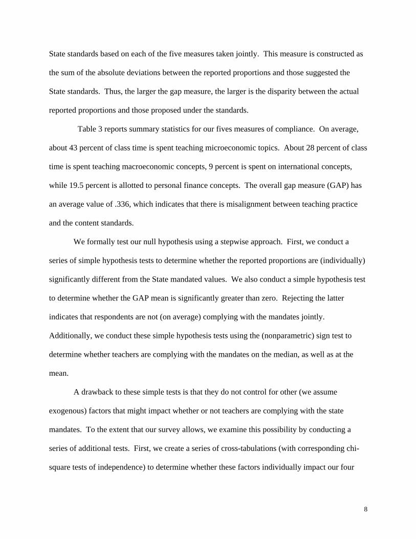
We formally test our null hypothesis using a stepwise approach. First, we conduct a

series of simple hypothesis tests to determine whether the reported proportions are (individually)

significantly different from the State mandated values. We also conduct a simple hypothesis test

to determine whether the GAP mean is significantly greater than zero. Rejecting the latter

indicates that respondents are not (on average) complying with the mandates jointly.

Additionally, we conduct these simple hypothesis tests using the (nonparametric) sign test to

determine whether teachers are complying with the mandates on the median, as well as at the

mean.

A drawback to these simple tests is that they do not control for other (we assume

exogenous) factors that might impact whether or not teachers are complying with the state

mandates. To the extent that our survey allows, we examine this possibility by conducting a

series of additional tests. First, we create a series of cross-tabulations (with corresponding chi-

square tests of independence) to determine whether these factors individually impact our four

8

proportional measures. Because cross-tabulations require discrete data, we decompose each of

our four proportional measures into two categories: those teachers who report that the proportion

of time meets or exceeds State standards, and those whose proportion falls short of the

standards.4 For the GAP variable (which cannot easily be decomposed into discrete

classifications) we utilize one-way (nonparametric) ANOVA to conduct a similar series of tests.

Lastly, we utilize regression techniques to determine whether these exogenous factors

jointly impact compliance (or non-compliance).5 Because none of our five compliance measures

are likely to meet the criteria for consistent estimation via ordinary least squares (OLS), we

choose to utilize limited dependent variable techniques. For each of our four proportional

measures, we employ a binary logit model, where the dependent variable of interest takes a value

of one if the reported proportion meets or exceeds State guidelines and a zero otherwise.

Transforming the GAP variable is more problematic, because it is less easily categorized

into discrete classifications. As before, we choose an approach that is both parsimonious and

consistent with our prior analysis. Specifically, we sort the data from smallest to largest and

create a series of binary variables that distinguish the observations based on quartiles. Each

dummy variable gives a value of one if an observation falls into a particular quartile, and zero

otherwise. Since a higher value for GAP implies more extreme divergence from the standards,

those observations in the first quartile are relatively close to full compliance, while those in the

fourth quartile are not close to compliance.6 Each of these dummy variables can be used as the

dependent variable in a binary logit regression to determine whether the exogenous factors

significantly and jointly impact compliance. Finally, we create a stepwise variable (or ordered

ranking variable) that combines these four dummy variables into a single, discrete variable. This

metric gives a value of zero if an observation for GAP is in the first quartile, a value of one if it

9

falls in the second quartile, and so on. This allows us to combine the information from the

previous four regressions into a single equation, which can be estimated with an ordered logit

model.

Our interpretation of these regression analyses is twofold. First, by examining the chi-

square tests for model significance (where the null hypothesis is that the regression does not

provide any additional information than the basic descriptive statistics and hypothesis tests); we

can determine whether controlling for these exogenous factors jointly influence compliance. If

we fail to reject the test for model significance, then the results presented in the simple

hypothesis test can be interpreted as robust, even when controlling for these exogenous

characteristics. Secondly, if we reject this hypothesis we can examine the signs and significance

of the coefficient estimates to determine which factors significantly influence compliance,

holding the other regressors constant.

All regression equations utilize the same set of independent variables, which represent

various teacher (and school) attributes and perceptions that have been identified as important

influences on student achievement in the economics education literature. These include: CORE

40, NCEE, JA, ICEE, UNEC, NOTIME, STMOT, GENDER, TEXP, PCTDV, INSERV,

SMALL, LARGE and EXTRA-LARGE. The rationale(s) for including each independent

variable are as follows. Teachers responsible for teaching a college preparation economics class

(CORE 40) are presumed to be more familiar with guidelines for topic coverage. Use of the

National Council on Economic Education (NCEE), Junior Achievement (JA), and/or Indiana

Council on Economic Education (ICEE) materials serve as another indication of the awareness

of relevant information pertaining to economics content standards.

10

Undergraduate training in economics (UNEC) is expected to influence compliance since

a greater awareness of content standards is likely to lead to a smaller gap between classroom

instruction and the expected allocation implied by content standards. Teachers indicating time

management issues (NOTIME) related to the implementation of content standards can be

expected to be more sensitive to over or under-coverage of the topics listed in the content

standards. The importance of student effort and interest in economics has also been identified as

a key determinant of the learning process, since student motivation can serve to undermine the

learning process. Thus, perceived challenges in motivating students (STMOT) may adversely

affect the alignment of topic coverage with prescribed coverage in the content standards.

The experience of teachers, both overall and in economics instruction (TEXP and

PCTDV) is predicted to have a favorable impact on adjusting to economics content standards, as

should attending a workshop provided by one of the councils on economic education (INSERV).

We have no a priori expectations about the relationship between content coverage and gender or

school size.

Empirical Results

The results for the simple hypothesis tests are contained in Table 4. Mean values indicate

that teachers spend slightly less time teaching micro and international topics relative to the

standards, and slightly more time teaching macro and personal finance topics. Analysis of the

parametric tests indicates that the (mean) proportions of time spent teaching microeconomics;

macroeconomics and international economics topics are not statistically different from the State

standards. However, the proportion of time spent teaching personal finance is significantly

different (and above) the standard. The GAP variable is also significantly greater than zero at

95% confidence or better. These results imply that, at the mean, teachers are “shaving” the

11

proportion of time spent teaching economics, particularly micro and international economics

(such that they do not deviate too far from the standards), and re-allocating that time to personal

finance topics.

The nonparametric tests presented in Table 4 not only reinforce the results of the

parametric tests, but also do so with a higher degree of statistical significance. Approximately

80 percent of the teachers in the sample spend less time (relative to the State standards) teaching

microeconomics, and 74 percent spend less time on international economics. Conversely, this

time is spent teaching personal finance. Moreover, as evidenced by the GAP variable, every

teacher in the sample deviates from the standards to some extent. A plausible interpretation of

these results is that while virtually all teachers in the sample deviate from the standards, they do

so in a predictable fashion. Additionally, when they do deviate, they are careful (at least on

average) about the magnitude (or proportion of total class periods) from which they deviate from

the individual standards.

As a robustness check, we also ran a nonparametric test with the null hypothesis that the

population median for the GAP variable was equal to the sample mean (0.336). The results show

that we reject the null at better than 95% confidence. This finding provides two insights. First, it

supports our earlier assertion that teachers are deviating from the standards. Second, rejecting

this test indicates (but does not conclusively prove) that the distribution of the GAP variable is

non-normal. As such, when conducting analysis of variance on the GAP variable, it is necessary

to resort to nonparametric techniques (i.e., the Mann-Whitney analog to ANOVA).

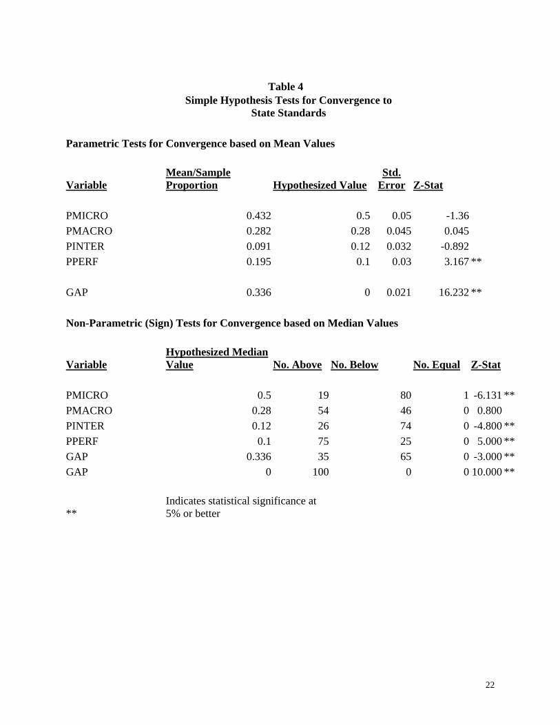
Table 5 presents the cross-tabulations and chi-square tests of independence between our

proportional variables and several exogenous variables. We find no significant relationship (i.e.,

we fail to reject the null hypothesis of independence) between failing to meet (or

12

meeting/exceeding) the standards and whether or not teachers used NCEE or Junior

Achievement materials, the number of undergraduate credit hours in economics earned by each

teacher, perceived lack of student interest, gender, years of teaching experience, the percent of

that experience spent teaching economics, whether the teacher attended an economic education

workshop, and the size of the school.

We do, however, find a number of factors that significantly influence whether a teacher

fails to meet the standards. First, respondents who do not teach a Core 40 course are more likely

to exceed the personal finance standard and less likely to meet or exceed the macro standard than

those who do teach a Core 40 course. Additionally, teachers who do not use materials sponsored

by the Indiana Council of Economic Education are more likely to spend too much time on

personal finance topics. Perhaps more importantly, teachers who indicated that time is not a

major factor in covering all of the standards are more likely not to meet those standards. The

implication of the latter is that the breadth and depth of content teachers are expected to cover

under the standards is not a significant determinant of whether those standards are met. That is,

the standards to not appear to be taxing in terms of the amount of time necessary to meet them.

It remains to be seen from more detailed analysis whether this preliminary finding is upheld.

Table 6 contains the results from a series of nonparametric ANOVA (Mann-Whitney)

tests for the GAP variable. Unlike the cross-tabulations that examined compliance for each of

the core competency areas individually, the Mann-Whitney test indicates whether certain factors

jointly influence compliance with the standards. The tests indicate that two of the factors

outlined in Table 5 significantly influence joint compliance. Specifically, teachers administering

a Core 40 course exhibit less deviation from the standards than those not teaching such a course,

and those teachers who use National Council on Economic Education materials exhibit less

13

deviation from the standards than those who do not use such materials. The first of these results

upholds the findings from our cross-tabulation analysis, while the latter is a new result arising

from aggregating compliance (or a lack thereof) across all four areas.

The regression results are reported in Tables 7 and 8. We begin by examining the chi-

square tests for model significance. Clearly, we fail to reject the null hypothesis (that controlling

for these exogenous characteristics provides no additional information than the simple

descriptive statistics) with 95% confidence for every equation in Tables 7 and 8. Thus, we

conclude that our simple hypothesis tests from Table 4 are robust, even when controlling for

these variables jointly. In other words, when taken in tandem, none of the exogenous

characteristics are significant determinants of compliance with the state standards. Given the

sparse number of significant coefficient estimates, this result is not surprising. However, it is

interesting (merely as an exercise) to note that the few significant coefficient estimates do

coincide with some of our previous findings. For example, teachers administering a CORE 40

course are more likely to meet or exceed the macroeconomics standards, and are also less likely

to have extreme GAP values (indicating divergence from the standards taken jointly). The

regressions also indicate that teachers working in larger schools are more likely to adhere to the

State standards (as evidenced by the logit regression for the GAP, first and second quartile

dummy variables). Greater teacher experience also has a positive impact on whether the

macroeconomics standard is met. Perhaps most intriguing is the finding that teachers reporting

that student motivation is a major challenge are more likely to adhere closely to the standards,

both overall (as evidenced by the GAP regressions), and to the microeconomics standard

individually.

14

Conclusion

From a policy perspective, our findings present a surprisingly optimistic picture about the

response of high school teachers to the adoption of state economic standards. We find that while

virtually all teachers in our sample deviate from the standards, the magnitude of the deviation is

small, and occurs in a predictable way. Most teachers appear to spend slightly less time on

microeconomics (43.2% versus the mandated 50%) and international economics concepts (9.1%

versus the mandated 12%) in favor of additional personal finance topics (19% versus 10%).

Moreover, our regression analysis indicates that this finding is robust to many exogenous factors

that are purported to influence a teacher’s decisions over course content. As a result, the

standards appear to be moderately successful in achieving its intended goal of creating

convergence in content coverage in high school economics curricula.

Successfully aligning economics instruction with state standards is dependent upon

altered teacher behavior. The findings of this paper suggest that there may interventions that can

lead to altered behavior by teachers. The lack of significance of demographic factors suggests

that these interventions may be workable under various demographic profiles for teachers of

economics courses. A key focus of these interventions would be to build awareness of standards

coverage through curriculum planning as well as through the activities of organizations such as

the NCEE, upon which the Indiana standards are based. It may also be useful for educators to be

aware of the extent to which standards have been adequately implemented in the classroom, prior

to the proposed economics assessment of high school students (such as the 2006 National

Assessment of Educational Progress (NAEP) Economics Assessment).

Given our finding that teachers behave in a predictable fashion, changing the standards

themselves may be another viable way to achieve that goal. For example, if policy makers want

15

exactly 50% course content in microeconomics, they may actually want to increase the

microeconomics standard (for example, to 56%) and reduce the personal finance standard (to,

say, 8%) knowing that teachers will deviate from the standard, but only marginally so. Future

work that empirically estimated the magnitude of this tradeoff (between personal finance and

microeconomics/international economics) would provide valuable information about the

effectiveness of such a policy.

The underlying motivation for this paper comes from the hypothesis that deviations

between actual content coverage and state mandates may contribute to a lack of economic

literacy in high school students. The results of our analysis do not support this claim, as teachers

appear to be (for the most part) adhering to the standards. However, the aggregate nature of our

data does not allow us to answer this question definitively. Instead, it provides direction for

future research. If teachers are spending the correct proportion (or something close to the correct

proportion) of time on each content area, the determinants of economic literacy should focus not

on what is being taught, but how it is being taught. Additionally, while teachers may be

spending an appropriate amount of time on each content area, the allocation of time spent on

individual topics within each content area may not be appropriate to ensure that students grasp

the major concepts central to economic literacy. As such, future research is necessary to identify

the allocation of time spent on individual concepts. This allows policy makers to subsequently

create standards at the level of the concept, and not the subject area, which enhance economic

literacy.

16

References

Indiana State Board of Education (2001). Indiana’s Academic Standards, Social Studies: Economics. Indianapolis, IN: Author Indiana State Board of Education, Division of Teacher Education and Certification. Bulletin 400. (Issued 1963; Revised 1969). 35. Indiana State Board of Education, Division of Teacher Education and Certification. Rule 46-47. (Issued 1984), 22. National Council on Economic Education (2003). Survey of the States: Economic and Personal Finance Education in our Nation’s Schools in 2002 – A Report Card. New York: Author. National Council on Economic Education (1997). Master Curriculum Guide in Economics: A Framework for Teaching the Basic Concepts. New York: Author. National Council on Economic Education (1997). Voluntary National Content Standards in Economics. New York: Author. Valentine, Gregory P. and Quddus, Munir (1998). A Status Report of Indiana’s High School Economics: Survey Results. In Jean V. Poulard (Ed.) Journal of the Indiana Academy of the Social Sciences. The University of Indianapolis, Indianapolis, IN, pp. 52-58. VanFossen, Phillip and McGrew, Chris (2002). Data on the Nature of the High School Economics Course in Indiana and the Economic Literacy of Indiana High School Students. A summary Report to the George and Frances Ball Foundation. Indiana Council on Economic Education: West Lafayette, IN. Walstad, William B. (1992). Economics Instruction in High Schools. Journal of Economic Literature, 30, pp. 2019-2051. Walstad, William B. (2001). Economic Education in U.S. High Schools. Journal of Economic Perspectives. Summer (2001). 15, 3, pp. 195-208. Walstad, William B. and Rebeck, Ken(2000). The Status of Economics in the High School Curriculum. Journal of Economic Education. 31, 1, pp. 95-101. Walstad, William B. and Soper, John C (1988). What is High School Economics? Factors Contributing to Student Achievement and Attitudes. Journal of Economic Education. Winter (1988), 20,1, pp. 23-38.

17

Table 1

Variable Names and Descriptions

Variable Name Description

PMICRO Proportion of class periods spent on microeconomic topics PMACRO Proportion of class periods spent on macroeconomic topics PINTER Proportion of class periods spent on international topics PPERF Proportion of class periods spent on personal finance topics GAP Joint difference between actual allocation of class periods and allocation prescribed by state content standard AGE Age of teacher in years TEXP Years of teaching experience ECEXP Years teaching experience in economics UNEC Hours of undergraduate economics courses GREC Hours of graduate economics courses GENDER 1 if male ECMAJ 1 if teacher undergraduate major is economics INSERV 1 if teacher attended a program/workshop sponsored by the Indiana Council on Economic Education or a local Center for Economic Education NOTIME 1 if teacher indicated that time to meet standards/cover material is a major challenge CORE 40 1 if respondent teaches a college prep economics class STMOT 1 if a lack of student interest in economics is a primary challenge for teacher ETEACH Number of economics courses presently being taught JA 1 if respondent indicated the use of Junior Achievement Materials ICEE 1 if respondent indicated the use of Indiana Council on Economic Education Materials PETEACH Proportion of years teaching spent teaching economics.

SMALL 1 if school’s size is between 0 and 500 students

MID-SIZE 1 if school’s size is between 501 and 1000 students

LARGE 1 if school’s size is between 1001 and 1500 students

EXTRA-LARGE 1 if school’s size is greater than 1500 students

PCTDV 1 if greater than 50% of a teacher’s experience is spent teaching Economics

18

Table 2 – Teacher Demographics Description Percentage Gender Male 75% Female 25% Age Distribution 24 – 29 5% 30 – 39 17% 40 – 49 34% 50 – 59 38% 60 - 69 6% Experience: Number of Years Teaching

1 – 9 23% 10 – 19 16% 20 – 29 33% 30 – 39 24% 40 - 49 4% Description Percentage Experience: Number of Years Teaching Economics

1 – 9 46% 10 – 19 28% 20 – 29 14% 30 – 39 11% 40 - 49 1% Undergraduate Degree B.A or B.S 100% Year of Undergraduate Degree Before 1984 72% After 1984 28% Undergraduate Major Social Studies 63% Business Education 14% Economics 6% Other 17% Social Studies Supporting Area History 72% Economics 72% Government 59% Western Civilization 37% Secondary Social Sciences 28% Geography 28% Psychology 19% Other 13%

19

Table 2 Continued Graduate Degree Masters’ Degree 82% No Graduate Degree 18% Year Graduate Degree Obtained Before 1984 61% After 1984 39% Graduate Major Secondary Education 69% School Administration 4% Other 27% Graduate Major: Percent with Emphasis Area

Social Studies 44% History 37% Economics 36% Government 20% Business Education 17% Sociology 15% Psychology 12% Political Science 11% Geography 8% Other 8%

20

Table 3 Summary Statistics for Variables used in the Analysis Variable Mean Median Std. Deviation PMICRO 0.432 0.422 0.103PMACRO 0.282 0.288 0.098PINTER 0.091 0.091 0.046PPERF 0.195 0.179 0.137GAP 0.336 0.283 0.207AGE 46.580 47.5 9.971GENDER 0.750 1 0.435TEXP 20.900 22 11.456ECEXP 12.910 10 9.874ECMAJ 0.060 0 0.239CORE40 0.650 1 0.479UNEC 11.970 12 6.389GREC 3.020 0 4.662NCEE 0.390 0 0.490JA 0.400 0 0.492ICEE 0.520 1 0.502NOTIME 0.380 0 0.488STMOT 0.320 0 0.469ETEACH 1.220 1 0.462PETEACH 0.639 0.667 0.293INSERV 0.650 1 0.479UNECDV 0.550 1 0.500TEXPDV 0.640 1 0.482PCTDV 0.600 1 0.492SMALL 0.21 0 0.409MID-SIZE 0.32 0 0.469LARGE 0.23 0 0.423EXTRA-LARGE 0.24 0 0.429 Number of Observations 100

21

22

Table 4

Simple Hypothesis Tests for Convergence to

State Standards Parametric Tests for Convergence based on Mean Values

VariableMean/Sample Proportion Hypothesized Value

Std. Error Z-Stat

PMICRO 0.432 0.5 0.05 -1.36 PMACRO 0.282 0.28 0.045 0.045 PINTER 0.091 0.12 0.032 -0.892 PPERF 0.195 0.1 0.03 3.167 ** GAP 0.336 0 0.021 16.232 ** Non-Parametric (Sign) Tests for Convergence based on Median Values

VariableHypothesized Median Value No. Above No. Below No. Equal Z-Stat

PMICRO 0.5 19 80 1 -6.131 ** PMACRO 0.28 54 46 0 0.800 PINTER 0.12 26 74 0 -4.800 ** PPERF 0.1 75 25 0 5.000 ** GAP 0.336 35 65 0 -3.000 ** GAP 0 100 0 0 10.000 **

** Indicates statistical significance at 5% or better

Table 5 Cross-Tabulations and Chi-Square Tests of Independence

PMICRO

PMACRO

PINTER

PPERF

Variable Does Not Meets or Does Not Meets or Does Not Meets or Does Not Meets or Meet Exceeds Meet Exceeds Meet Exceeds Meet Exceeds Standard

Standard

Total

Standard

Standard

Total

Standard

Standard

Total

Standard

Standard

Total

No 29 6 35 22 13 35 27 8 35 4 31 35Core 40

Yes 51 14 65 24 41 65 47 18 65 21 44 65Total 80 20 100

46 54 100 74 26 100

25 75 100

Chi-Square Statistic

0.275

6.16 ** 0.276

5.289

**

No 50 11 61 31 30 61 47 14 61 14 47 61NCEE

Yes 30 9 39 15 24 39 27 12 39 11 28 39Total 80 20 100

46 54 100 74 26 100

25 75 100

Chi-Square Statistic

0.378

1.463

0.756

0.35

No 50 10 60 29 31 60 44 16 60 17 43 60JA Yes 30 10 40 17 23 40 30 10 40 8 32 40

Total 80 20 100

46 54 100 74 26 100

25 75 100

Chi-Square Statistic

1.042

0.329

0.035

0.889

No 39 9 48 23 25 48 37 11 48 8 40 48ICEE

Yes 41 11 52 23 29 52 37 15 52 17 35 52Total 80 20 100

46 54 100 74 26 100

25 75 100

Chi-Square Statistic 0.09 0.137 0.456 3.419 *

< 12 hours 36 9 45

22 23 45 31 14 45 10 35 45UNEC

=>12 hours

44 11 55 24 31 55 43 12 55 15 40 55Total 80 20 100

46 54 100 74 26 100

25 75 100

Chi-Square Statistic

0 0.275

1.111

0.337

No 53 9 62 26 36 62 45 17 62 15 47 62NOTIME

Yes 27 11 38 20 18 38 29 9 38 10 28 38Total 80 20 100

46 54 100 74 26 100

25 75 100

Chi-Square Statistic

3.067

* 1.085

0.171

0.057

No 56 12 68 33 35 68 49 19 68 17 51 68STMOT

Yes 12 8 32 13 19 32 25 7 32 8 24 32Total 80 20 100

46 54 100 74 26 100

25 75 100

Chi-Square Statistic

0.735

0.547

0.416

0

Female

20 5 25 11 14 25 20 5 25 7 18 25GENDER

Male 60 15 75 35 40 75 54 21 75 18 57 75Total 80 20 100

46 54 100 74 26 100

25 75 100

Chi-Square Statistic

0 0.054

0.642

0.16

<=15 years 28 8 36 20 16 36 26 10 36 9 27 36TEXP

> 15 years 52 12 64 26 38 64 48 16 64 16 48 64Total 80 20 100

46 54 100 74 26 100

25 75 100

Chi-Square Statistic

0.174

2.068

0.092

0

24

25

<=50% 34 6 40 17 23 40 30 10 40 12 28 40PCTDV

> 50% 46 14 60 29 31 60 44 16 60 13 47 60Total 80 20 100

46 54 100 74 26 100

25 75 100

Chi-Square Statistic

1.042

0.329

0.035

0.889

No 29 6 35 16 19 35 28 7 35 6 29 35

INSERV

Yes 51 14 65 30 35 65 46 19 65 19 46 65Total 80 20 100

46 54 100 74 26 100

25 75 100

Chi-Square Statistic

0.275

0.002

1.008

1.773

Small 18 3 21 11 10 21 17 4 21 3 18 21Mid-Sized

27 5 32 16 16 32 22 10 32 5 27 32

SIZE Large 17 6 23 8 15 23 17 6 23 9 14 23Extra-Large

18 6 24 11 13 24 18 6 24 8 16 24

Total 80 20 100

46 54 100 74 26 100

25 75 100

Chi-Square Statistic

1.719

1.716

0.999

6.124

* indicates statistical significance at the 10% level ** indicates statistical significance at the 5% level

Table 6

Mann-Whitney Tests Dependent Variable: GAP Decomposed by: n Mean Std. Deviation Test Statistic CORE 40 no 35 0.435 0.274 -2.464 ** yes 65 0.283 0.134 NCEE no 61 0.378 0.229 -2.226 ** yes 39 0.271 0.146 JA no 60 0.331 0.209 -0.654 yes 40 0.344 0.206 ICEE no 48 0.345 0.175 -0.866 yes 52 0.323 0.233 UNEC <= 9 hours 45 0.371 0.262 -0.391 > 9 hours 55 0.308 0.144 NOTIME no 62 0.357 0.236 -0.586 yes 38 0.303 0.145 INTEREST no 68 0.350 0.207 -1.526 yes 32 0.307 0.206 GENDER Female 25 0.361 0.237 -0.354 Male 75 0.328 0.196 TEXP <= 15 years 36 0.338 0.208 -0.417 > 15 years 64 0.336 0.208

27

Table 6 Continued Decomposed by: n Mean Std. Deviation Z-Statistic PCTDV <= 0.50 40 0.355 0.227 -0.549 > 0.50 60 0.324 0.193 INSERVIC no 35 0.354 0.189 -0.903 yes 65 0.327 0.216 SMALL no 79 0.325 0.207 -1.316 yes 21 0.380 0.203 MID-SIZE no 68 0.322 0.194 -1.035 yes 32 0.367 0.232 LARGE no 77 0.350 0.210 -1.364 yes 23 0.290 0.193 EXTRA-LARGE no 76 0.347 0.214 -1.041 yes 24 0.302 0.183 * indicates statistical significance at the 10% level ** indicates statistical significance at the 5% level

ble 7

Ta Logit Regression Results

Dependent Variable: PMICRO PMACRO PINTER PPREF Dummy Variable

Dummy Variable

Dummy Variable

Dummy Variable

Variable Estimated T-Stat

Estimated T-Stat Estimated T-Stat

Estimated T-Stat

Coefficient Coefficient Coefficient

Coefficient

Constant -4.532 -2.866 ** -1.166 -1.136 -2.010

-1.768 * -1.474 -2.203 **CORE 40 0.459 0.718 1.415 2.720 ** 0.114 0.210 0.663 1.099NCEE -0.165 -0.246 0.405 0.753 0.664 1.154 0.537 0.969JA 0.493 0.843 0.732 1.449 -0.181 -0.343 -1.131 -1.178ICEE -0.072 -0.076 0.150 0.195 -0.495 -0.600 -0.032 -0.728UNEC -0.023 -0.480 -0.008 -0.219 -0.003 -0.089 -0.574 -0.912NOTIME 1.733 2.170 -0.628 -1.135 -0.726 -1.237 -0.699 -1.060STMOT 1.664 1.991 ** 0.673 1.117 -0.892 -1.391 0.355 0.553GENDER -0.190 -0.271 -0.598 -1.016 0.522 0.810 0.002 0.087TEXP 0.039 1.340 0.050 2.232 ** 0.020 0.907 1.289 1.250PCTDV 0.892 0.857 -0.680 -0.817 0.728 0.794 0.083 0.085INSERV -0.275 -0.303 -0.481 -0.655 0.820 1.014 0.048 0.055SMALL 0.083 0.094 0.268 0.416 -0.652 -0.881 -0.797 -1.051LARGE 0.959 1.205 0.612 0.911 -0.397 -0.561 -0.727 -0.953

EXTRA-LARGE 0.924 1.179

0.017

0.026 -0.521 -0.745

Unrestricted Log-Likelihood -43.676 -59.535 -53.694 -47.766Restricted Log-Likelihood -50.040 -68.994 -57.306 -56.234Chi-Square Statistic (14 degrees of Freedom)

12.73

18.92 7.22

16.94

Number of Observations 100

100 100

100

* indicates statistical significance at the 10% level ** indicates statistical significance at the 5% level

30

Table 8: Logit

Regression

Results

GAP GAP GAP GAP GAPDependent Variable: Ranking Bottom Quartile Second Quartile Third Quartile Top Quartile Ordered

Dummy Variable

Dummy Variable

Dummy Variable

Dummy Variable

Variable

Estimated T-Stat

Estimated T-Stat Estimated T-Stat

Estimated T-Stat

Estimated T-StatCoefficient Coefficient Coefficient Coefficient

Coefficient

Constant 2.837 2.927 ** -2.913 -2.198 ** -1.415 -1.185 -1.576 -1.392 0.840 0.709CORE 40 -0.762 -1.814 * 0.301 0.514 0.657 1.148 0.509 0.877 -1.343 -2.371 **NCEE -0.230 -0.491 -0.221 -0.364 0.447 0.763 0.398 0.669 -0.933 -1.404JA 0.467 1.045 -0.544 -0.954 -0.026 -0.047 0.015 0.027 0.544 0.929ICEE -0.450 -0.662 0.521 0.573 0.370 0.418 -0.917 -1.076 -0.193 -0.203UNEC 0.009 0.267 -0.051 -1.080 0.040 0.980 0.005 0.123 -0.011 -0.253NOTIME -0.810 -1.661 * 0.496 0.758 0.420 0.682 -0.022 -0.038 -0.921 -1.453STMOT -1.388 -2.875 ** 1.083 1.666 * 0.761 1.190 -0.546 -0.816 -1.482 -1.968 **GENDER 0.145 0.298 -0.076 -0.119 0.530 0.770 -0.313 -0.497 0.026 0.041TEXP -0.009 -0.433 0.004 0.181 -0.020 -0.845 0.034 1.422 -0.026 -1.039PCTDV -0.326 -0.434 0.797 0.831 -0.811 -0.873 0.337 0.365 -0.277 -0.285INSERV 0.309 0.462 -0.260 -0.292 -0.121 -0.144 0.195 0.249 0.433 0.483SMALL 0.212 0.333 0.920 1.054 -0.983 -1.326 -0.460 -0.654 0.755 1.015LARGE -0.637 -0.982 1.951 2.373 ** -1.579 -2.073 ** -0.239 -0.338 0.089 0.107EXTRA-LARGE -0.511 -0.841

1.940 2.343

** -1.229 -1.664

* -0.763 -1.012

0.427 0.562

Unrestricted Log-Likelihood -129.267 -48.467 -51.029 -52.754 -47.012 Restricted Log-Likelihood -138.629 -56.234 -56.234 -56.234 -56.234 Chi-Square Statistic (14 dof) 18.73 15.53 10.41 6.96 18.44 Number of Observations

100 100 100

100

100

* indicates statistical significance at the 10% level ** indicates statistical significance at the 5% level

Endnotes

1 Within Indiana’s Economic standards, the following standards and benchmarks can be

associated with personal finance issues. Standard 1, “Scarcity and Economic Reasoning”, two

benchmarks can be identified as those dealing in personal finance: (1) “Formulate a savings or

financial investment plan for a future goal” and (2) “Predict how interest rates will act as an

incentive for borrowers and savers.” In Standard 2, the “Supply and Demand” benchmark

dealing with personal finance reads, “Explain how financial markets, such as the stock market,

channel funds from savers to investors”. In Standard 4, “The Role of Government”, the personal

finance benchmark statement reads, “Identify taxes paid by students. In Standard 5, “National

Economic Performance”, the personal finance benchmark statement reads, “Analyze the impact

of inflation of students’ economic decisions.” Standard 6, “Money and the Role of Financial

Institutions”, identifies four benchmarks that deal with personal finance: (1) “Explain the role of

banks and other financial institutions in the economy of the United States”, (2) “Compare and

contrast credit, savings, and investment services available to the consumer from financial

institutions”; (3) “Research and monitor financial investments, such as stocks, bonds, and mutual

funds”; and (4) “Formulate a credit plan for purchasing a major item comparing different interest

rates.” Standard 7, “Economic Stabilization” has a benchmark that reads, “Articulate how a

change in monetary or fiscal policy can impact a student’s purchasing decision.”

2 394 to public high school teachers and 36 to private high school teachers

3 Even though only 6 hours of economics courses were required prior to 1984, the vast majority

of teachers in our sample (70 percent) earned more than 6 hours of economic credit. In fact 55

percent of the sample actually earned 12 or more credit hours in economics.

4 As the results in Table 4 show, only one reported value is exactly equal to the state standards.

As such, including the observations who exactly meet the standards with those who exceed the

standards (as opposed to including them with those who do not meet the standards) causes little

loss of generality. Also, we chose to use cross-tabulations (as opposed to an approach such as

the Mann-Whitney test) because we believe that it expresses the same information, yet is also

more consistent with the coming regression analysis.

5 Because our survey does not provide data to control for all important determinants of

compliance, our results may suffer from omitted variable bias. As such, our intent in Tables 7

and 8 is simply to perform an exploratory analysis with the data at our disposal.

6 The Mann-Whitney test employed to analyze the GAP variable prior to the regression analysis

essentially operates by ranking the data and comparing rankings across the treatment variable(s).

As such, our decision to categorize the GAP variable by quartiles is consistent with our previous

analysis.

32