A Real-Time Gridded Crop Model for Assessing Spatial Drought Stress onCrops in the Southeastern United States

RICHARD T. MCNIDER,* JOHN R. CHRISTY, DON MOSS, KEVIN DOTY, AND CAMERON HANDYSIDE

Earth System Science Center, University of Alabama in Huntsville, Huntsville, Alabama

ASHUTOSH LIMAYE

NASA Marshall Space Flight Center, Huntsville, Alabama

AXEL GARCIA Y GARCIA

Research and Extension Center, University of Wyoming, Powell, Wyoming

GERRIT HOOGENBOOM

Department of Biological and Agricultural Engineering, The University of Georgia, Griffin, Georgia

(Manuscript received 19 January 2010, in final form 21 January 2011)

ABSTRACT

The severity of drought has many implications for society. Its impacts on rain-fed agriculture are especially

direct, however. The southeastern United States, with substantial rain-fed agriculture and large variability in

growing-season precipitation, is especially vulnerable to drought. As commodity markets, drought assistance

programs, and crop insurance have matured, more advanced information is needed on the evolution and

impacts of drought. So far many new drought products and indices have been developed. These products

generally do not include spatial details needed in the Southeast or do not include the physiological state of the

crop, however. Here, a new type of drought measure is described that incorporates high-resolution physical

inputs into a crop model (corn) that evolves based on the physical–biophysical conditions. The inputs include

relatively high resolution (as compared with standard surface or NOAA Cooperative Observer Program

data) (5 km) radar-derived precipitation, satellite-derived insolation, and temperature analyses. The system

(referred to as CropRT for gridded crop real time) is run in real time under script control to provide daily

maps of crop evolution and stress. Examples of the results from the system are provided for the 2008–10 growing

seasons. Plots of daily crop water stress show small subcounty-scale variations in stress and the rapid change in

stress over time. Depictions of final crop yield in comparison with seasonal average stress are provided.

1. Introduction

The severity of drought has many implications for so-

ciety, including its impacts on the water supply, water

pollution, reservoir management, and ecosystem. How-

ever, its impacts on rain-fed agriculture are especially

direct. The development of information that relates the

impacts of drought to agriculture has been a key com-

ponent of disaster management and crop yield estimates

for the agricultural community. In the United States,

drought classifications such as the Drought Monitor

(Svoboda et al. 2002; information also available online

at http://drought.unl.edu/dm/monitor.html) have a ma-

jor impact on disaster assistance payments and special

relief programs as well as eligibility for assistance un-

der agricultural programs such as the U.S. Department

of Agriculture’s (USDA) Agricultural Water Enhance-

ment Program (AWEP). Because of the importance of

drought, there have been many attempts to characterize

its severity, resulting in the numerous drought indices that

have been developed (Heim 2000; Niemeyer 2008).

* Current affiliation: AgWeatherNet, Washington State Uni-

versity, Prosser, Washington.

Corresponding author address: Richard T. McNider, Earth System

Science Center, University of Alabama in Huntsville, Huntsville,

AL 35899.

E-mail: mcnider@nsstc.uah.edu

JULY 2011 M C N I D E R E T A L . 1459

DOI: 10.1175/2011JAMC2476.1

� 2011 American Meteorological Society

The basis of a drought index is to assess the avail-

ability of water for a particular or general use at a given

time. This can be done using budget models that track

gains and losses of water or from inferring soil moisture

from auxiliary information such as temperature (Wetzel

1984; McNider et al. 1994; Norman et al. 1995), or the

greenness of vegetation (Sellers 1985; Kogan 1995, Brown

et al. 2008), or combinations of the above (Carlson et al.

1994; Nemani and Running 1989). Early drought indices

relied on a water budget. The Palmer drought severity

index (PDSI; Palmer 1965; Alley 1984) was originally

based primarily on coarse rain gauge precipitation for

gain and a simplified evaporation calculation based on

temperature for losses to accrue a drought status for

large areas (originally climate divisions on the order of

10 000–500 000 km2). It was recognized that the PDSI,

while perhaps capturing a longer definition of drought,

failed to respond quickly to drought stress on crops that

were primarily responding to moisture sometimes in the

first few inches of top soil. Palmer (1968) developed a

shorter-term index called the crop moisture index (CMI).

While the PDSI and CMI can accept higher-resolution

inputs, they have primarily been driven by the National

Weather Service (NWS) Cooperative Observer Program

coarse-resolution data for rainfall and soil character-

istics and retained the simplified evaporative loss

parameterization.

As measures of drought intensity became the basis of

important societal decisions from drought response

plans to eligibility for relief programs, the need for finer-

scale and more accurate measures of specific types of

droughts (Wilhite and Glantz 1985) increased. In re-

sponse to this need, many new drought indices have

been developed (Heim 2000; Niemeyer 2008). Keyantash

and Dracup (2002) provide a robust summary of drought

indices, their basis, and performance. Some of the more

advanced approaches estimate direct physical losses

(transpiration; Senay 2008) and runoff (Narasimhan and

Srinivasan 2005). Because drought can be highly lo-

calized, satellite data with high spatial resolution

compared to standard in situ data have been employed.

Anderson et al. (2007) and Anderson et al. (2011) utilized

a combination of geostationary and polar-orbiting data

to recover model root-zone moisture within a simple

boundary layer. One of the more advanced examples

is the soil moisture deficit index (SMDI) developed by

Narasimhan and Srinivasan (2005). Recognizing the crit-

ical role of soil moisture and its spatial variability in ag-

ricultural losses, Narasimhan and Srinivasan (2005) used

the framework of a hydrological model (Soil and Water

Assessment Tool, or SWAT) to determine soil moisture.

SWAT is a basin-scale hydrologic model that incorpo-

rates spatial variability in terrain, soil characteristics,

and rainfall (see Arnold et al. 1998). Narasimhan and

Srinivasan (2005) used the root zone moisture averaged

over a 7-day period to develop a soil dryness that could

be compared against long-term soil dryness from his-

torical runs. This provided a natural method for putting

a drought period into some historical context. The

derived soil moisture index compared well to selected

locations of satellite-derived greenness (Sellers 1985).

Recently, Senay (2008), using a combination of radar-

derived high-resolution precipitation and high-resolution

land-use estimates of evapotranspiration (ET), provided

a 5-km estimate of vegetative ET (VegET) for the United

States. For agricultural land, they employed relation-

ships for generic cereal crops for several stages of devel-

opment. The present investigation uses a direct approach

to crop physiology by employing a specific crop model

and utilizes satellite data to determine insolation as a

driver of ET.

The present investigation builds upon the ideas of

Narasimhan and Srinivasan (2005) and Senay (2008) to

conceptualize and construct a system that can capture

the high-resolution impacts of drought on specific crop

agricultural production. It moves beyond the approach

of soil moisture being a correlative measure of agri-

cultural loss to a direct computation of specific crop

responses to water availability. This is accomplished by

directly running a crop model [the Climate System Model

(CSM)–Clouds and the Earth’s Radiant Energy System

(CERES)–Maize model of the Decision Support System

for Agrotechnology Transfer (DSSAT); see below] in

real time at high spatial resolution. We will refer to this

real-time crop model as CropRT (for gridded crop real

time). In the SMDI, only a generic plant biomass model

was used, and in VegET, water uptake relations were

used for a generic cereal crop. The CropRT further in-

corporates radar-derived precipitation that had been

envisioned by Narasimhan and Srinivasan (2005) for use

in SWAT and includes high-resolution satellite estimates

of insolation, which is a critical component of biomass

production and water loss. While DSSAT provides ad-

ditional details on plant and local soil moisture inter-

action, it does not accumulate or spatially aggregate

runoff. Given the rapid advancements in remote sens-

ing, there are now many opportunities for linking crop

models with remotely sensed data for both historical anal-

ysis and yield forecasting (Hoogenboom 2000; Bannayan

et al. 2003; Fang et al. 2008).

The following describes the system and its potential

uses. Major emphasis is given to high spatial variabilities

in rainfall, temperature, and insolation that have been

incorporated into the model. In this prototype setting,

we have not included the spatial variation in soil char-

acteristics that is needed to further advance and refine

1460 J O U R N A L O F A P P L I E D M E T E O R O L O G Y A N D C L I M A T O L O G Y VOLUME 50

the system. The spatial variability of the local soil pa-

rameters and soil profiles needed for DSSAT is cur-

rently under development and will be reported upon

later. The goal of this paper is to present a prototype

of a real-time crop model and the potential that such

a system might have for estimating agricultural drought

effects and for projecting crop yield through the growing

season. Because of the omission of spatial variation in

soil characteristics, the gridded crop model provides an

interesting display of the variation in stress and yield

entirely due to both the temporal and spatial variabil-

ities of weather.

2. Development of high-resolution droughtproducts in the Southeast

The NWS Cooperative Observer Program’s irregular

coverage amounts to a much coarser resolution than

5 km, which can be achieved with remotely sensed

datasets. Here, we refer to the 5-km resolution as the

high-resolution product. In the Southeast (SE), small-

scale air mass convection is often the major source of

growing-season rainfall. Additionally, soil characteristics

vary on extremely small spatial scales. Thus, significant

variations in soil moisture can occur on the subcounty

scale and even the subfarm scale. Unlike the West, which

is largely insulated from drought by irrigation and the

Midwest, which is partially immune to short-term drought

by deep-water-holding soils, the SE is sensitive to droughts

even on the scale of a week due to its relatively poor

water-holding capacity of soils, especially for the coastal

plain region.

To capture some aspects of this finescale drought,

a lawn and garden index (LGI) was developed using

high-resolution radar-derived precipitation. The origi-

nal LGI was developed by the Alabama Office of State

Climatology and was expanded to Florida and Georgia.

It is a semi-empirical attempt to characterize the current

soil moisture in its capacity to sustain healthy lawns and

gardens. The index is computed in two stages.

First, an estimate is made on how much recent pre-

cipitation contributes to current soil moisture. It as-

sumes that any precipitation over the past 21 days

should be included in the computation. It also assumes

that more recent precipitation is more significant than

less recent events. All precipitation during the previous

7-day period is considered to be equally important, but

precipitation before that time is discounted according

to a linear sliding scale. A more robust soil water model

is needed here. The key input in this product, which

differs from most large-scale analyses, is that the pre-

cipitation used is radar-derived precipitation at nearly

5-km resolution. Thus, finescale (almost to the farm

scale) data are available to define small-scale droughts.

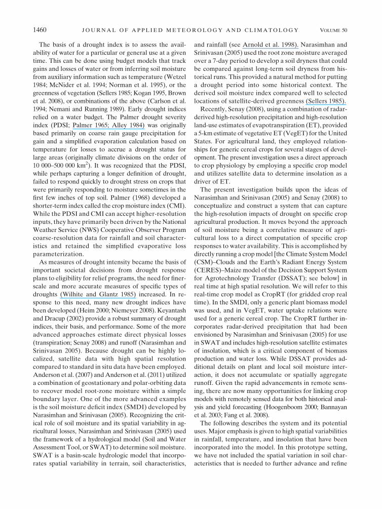
Second, an estimate is made of average water require-

ments for the current day. The LGI uses a simple daily

mean annual cycle of ‘‘needs amount,’’ varying from

10 mm during the winter and ramping to 50 mm during

the summer for the 21-day tapered index input, based

on shallow rooted vegetation responses to rainfall.

The needs amount is a critical weakness in the system.

The needs amount depends on the specific crop and

phenological state of the plant. The difference between

the water needs and the current effective rainfall from

above is the daily lawn-and-garden moisture index

(in inches). Figure 1 shows an example of the LGI for

the SE.

While the empirical approach of the LGI has grossly

simplifying assumptions, its inclusion of the key input

of high-resolution precipitation and physical units of

moisture deficit has made it a highly effective and useful

tool in conveying spatial characteristics of agricultural

drought to decision makers. It was expanded from Alabama

to Georgia and Florida under a Southeast Climate Con-

sortium (SECC) activity and was integrated into the

SECC’s AgroClimate Web site (www.AgroClimate.org)

delivery system (Fraisse et al. 2006).

FIG. 1. Example of the LGI for 28 Jul 2008 (in.).

JULY 2011 M C N I D E R E T A L . 1461

The success of the LGI and its use by the Drought

Monitor to refine drought categories at the county and

even subcounty levels has led to the view that other high-

resolution drought products could have value to the ag-

ricultural community. The SECC had long embraced

crop models (e.g., DSSAT) to evaluate the impacts of

climate variability and seasonal climate forecasts on ag-

ricultural yields (Garcia y Garcia et al. 2006; Paz et al.

2007). Thus, it was planned to merge components of

the LGI with the DSSAT crop models to provide high-

resolution information on drought stress for the critical

agronomic crops of the SE.

In looking at prior agricultural drought indices, it was

felt that three aspects were important to the develop-

ment of a more useful agricultural drought product in

the SE.

1) Use of high-resolution radar-derived precipitation:

The coarse spacing of Cooperative Observer Pro-

gram rain gauges is not sufficient to capture the

rainfall variability during the growing season in the

SE. Available radar composites provide continual

spatial coverage at a resolution of 4.76 km 3

4.76 km or approximately 22 km2. Narasimhan and

Srinivasan (2005) had proposed this scale for the

SMDI but in their paper used interpolated rain-

gauge data. Senay (2008) used this precipitation prod-

uct in VegET.

2) Improved specification of water loss due to plant up-

take and surface evaporation: While the LGI included

the high-resolution radar-derived precipitation, its

treatment of water loss and water use were largely

heuristic and simple. The approach in Narasimhan

and Srinivasan (2005) of using a Penman–Monteith

method in the SWAT model (Ritchie 1972) provides

a more realistic water loss representation. However,

such an approach requires estimates of incoming net

energy, which drives the evaporative losses espe-

cially under full canopies. For historical cumulative

long-term drought studies, surrogates for incoming

energy based on sun angle and average cloudiness

have been used. However, for short-term results

actual daily incoming solar energy (insolation) is

desired. Surface observations of insolation are gen-

erally not available and surface-based cloud obser-

vations at high resolution are also not available.

Historically, only NWS first-order stations reported

cloud cover. Errors in insolation over short-term

periods, though perhaps less critical than precipita-

tion, can introduce errors in water loss. Satellite data,

however, can provide relatively robust measures of

insolation and these data are now becoming readily

available (see below). Thus, the preferred path was to

use Penman-type evaporation loss driven by satellite-

derived insolation. A simplification of the Penman-

type evaporation is contained within the DSSAT soil

moisture budget calculations (Priestley and Taylor

1972; Ritchie et al. 1998).

3) Incorporation of plant physiological stage and mois-

ture: The coincident moisture and phenological stage

of the plant are important to both water loss by the

soil through soil evaporation and plant transpira-

tion and to crop yield. The stage of the plant in

terms of canopy development and expansion is

important to the amount of water lost from the soil

by evapotranspiration. This canopy-dependent loss

was estimated in the SMDI SWAT system by the

use of a generic plant module. However, in some

crops, such as corn, there are times when the Pen-

man relationships for plant water needs using only

a mean canopy area fail. As an example, when corn

reaches maturity, it can retain water for kernel de-

velopment even though transpiration drops. Thus es-

timates of actual to potential evaporation based on the

canopy may not capture the real stress on the crop

yield.

In addition to the role of the plant in impacting water

loss, the root-zone moisture is also critical to plant

development and final yield. Plants do not simply

control water loss but are directed in their physio-

logical development by available water. Early avail-

able water may impact the number of leaves that are

initiated and potential leaf expansion, changing the

ultimate evapotranspiration potential of the canopy.

As another example, at the stage when corn is in the

kernel filling stage, final yield is not as sensitive to

moisture as in the pollination stage or in the physi-

ological decision stage for the number of kernels.

This is because at the final kernel growth stage the

plant will sacrifice water and nutrients to support

the kernel at the expense of the leaves and stalk.

But if the full complement of kernels is not set early

during reproductive development or if moisture is

insufficient for full pollination, the final yield will be

significantly impacted even if plenty of soil moisture is

available near the final maturity date (Ritchie et al.

1998). Other crops such as soybeans may not be as

sensitive since their phenological window for de-

cisions on yield may be longer and not as time critical.

To develop a system that would capture these three

desirable attributes requires 1) a crop model that iden-

tifies the various physiological stages of a plant, 2) high-

resolution radar data in real time, and 3) high-resolution

insolation values on a daily basis. The following sections

describe this system.

1462 J O U R N A L O F A P P L I E D M E T E O R O L O G Y A N D C L I M A T O L O G Y VOLUME 50

a. Crop model component

DSSAT is a computer software system designed to

predict growth and yield for more than 25 crops, and to

assist in producing successful crop management tech-

niques, and to provide alternate options for decision

making (Tsuji et al. 1998; Hoogenboom et al. 2004). The

DSSAT models use variables such as weather, soil type,

and soil profile properties, as well as cultivar-specific

inputs and management including irrigation and amount

and type of fertilizer among others for simulating

growth, development, and yield. DSSAT also has a soil

hydrological model that estimates soil water flow and

root water uptake as a function of soil surface and soil

profile properties (Ritchie et al. 1998; Jones et al. 2003).

The atmosphere can limit transpiration by low solar

radiation and cool temperatures, the canopy can limit it

by low leaf area index (LAI), and the soil can limit it by

low soil water content or low root length density. Each

simulation for a single growing season provides a large

amount of data output, including rooting depth, plant

transpiration, soil temperature and moisture, nitrogen

levels in soil, plant growth, and development, as well as

a final water, nitrogen, and carbon balance. The models

can be run for a single year or multiyear climate mode to

account for both the seasonal weather variability and in-

terannual climate variability (Thornton and Hoogenboom

1994; Garcia y Garcia et al. 2006).

SECC is a collaborative group of state climatologists,

agricultural researchers, atmospheric scientists, econo-

mists, anthropologists, and hydrologists in Alabama,

Florida, Georgia, and North Carolina. The SECC strongly

embraced the use of the DSSAT crop models as a method

to evaluate the value and utility of seasonal forecasts

and in crop management practices such as irrigation

through the use of long-term climatology (Paz et al.

2007).

b. High-resolution rainfall data

The coarse spacing of rain gauges compared to the

scale of convective precipitation events has lead to un-

certainties in the amount of rainfall at discrete points.

With the development of the national Next Generation

Doppler Radar (NEXRAD) network came the oppor-

tunity to establish a national radar-derived precipitation

product. Radar returns have the advantage of acquiring

information that relates to rainfall in an almost continuous

spatial and temporal domain. The NWS River Forecast

Centers (RFCs) took the lead in establishing procedures

to use this radar information to develop derived rainfall

products. The products are, in fact, a combination of ra-

dar information and rain gauge data. Using regional

radar–rainfall relationships in each of the 12 RFCs in

the continental United States, these relationships are

continually calibrated by automatic rain gauge data at

6-h intervals. This combined product is referred to as a

multisensor precipitation analysis. The 12 regional RFC

6-h rainfall products are collected into a continental

U.S. multisensor rainfall analysis product that is accu-

mulated to produce a 24-h (daily) continental U.S. rainfall

analysis on a nearly 5-km (4.7625 km) grid. (A complete

technical description is available online: http://www.emc.

ncep.noaa.gov/mmb/ylin/pcpanl/stage4/.)

This NOAA/NWS daily rainfall product is used as the

basic precipitation input to the LGI and into the gridded

crop mode system. It is automatically acquired and ar-

chived for this purpose by the Alabama Office of State

Climatologist.

c. Satellite-derived insolation

The University of Alabama in Huntsville (UAH) and

the National Aeronautics and Space Administration

Marshall Space Flight Center (NASA MSFC) have de-

veloped an operational system that uses the physical

retrieval method (Gautier et al. 1980; Diak and Gautier

1983) to employ Geostationary Operational Environ-

mental Satellite (GOES) visible imagery in recovering

insolation at high resolution (4-km grid) for use in regional-

scale models. These data are publicly available online

(http://satdas.nsstc.nasa.gov/). Satellite techniques are

relatively robust in their ability to recover surface values

of insolation. While there are other statistical techniques

for recovering insolation from GOES imagery (Tarpley

1979; Pinker et al. 2003), the physical retrieval technique

has advantages in that it calculates cloud transmittance

and absorption, which can then be incorporated in more

complex radiative transfer models (Pour-Biazar et al.

2007).

The amount of solar energy reaching the earth’s sur-

face (insolation) is estimated from the broadband visible

channel on GOES. It is desirable to estimate both direct

and diffuse radiation (scattering from the atmosphere

and clouds). The albedo of the surface is required to

accurately compute these components. The surface al-

bedo (for each hour) is calculated using a short-term

history of GOES visible channel reflectance measure-

ments from cloud-free images (minimum visible value

over the history), the solar constant, and an estimate of

the water vapor content of the atmosphere. In cloudy

regions, a historical estimate of the albedo (from cloud-

free data) is used. The procedure includes three pro-

cesses: 1) attenuation of the downward flux of solar

radiation in cloud-free regions by molecular scattering

and absorption by atmospheric water vapor, 2) absorption

and scattering of solar radiation by clouds, and 3) atten-

uation of solar radiation by the atmosphere below the

JULY 2011 M C N I D E R E T A L . 1463

clouds. Atmospheric absorption is calculated with a pa-

rameterized radiative transfer model appropriate for

shortwave radiation and is dependent on water vapor

(total precipitable water in our case) and satellite and

solar-viewing geometry. Cloud absorption is parameter-

ized solely on visible reflectance and Rayleigh scattering

with a molecular pathlength. A comparison to surface

pyranometers is found in McNider et al. (1995).

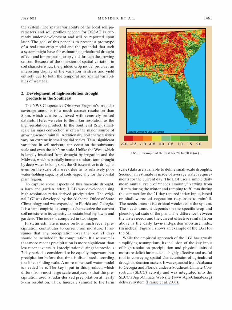
These insolation products have been applied in air

quality and weather forecast settings (McNider et al.

1994, 1995). The use of this insolation product was ex-

plored to improve the spatial specification of water loss

in the LGI. Figure 2 shows an example of the use of the

satellite-derived insolation values in estimating the evapo-

transpiration loss based on insolation using the Priestley

and Taylor (1972) formulation. The spatial variation in

estimated evapotranspiration shows that on short time

scales these variations may impact the spatial distribu-

tion of soil moisture. The 4-km insolation product used

here and in DSSAT is based on hourly GOES images

but only a single daily value of average insolation is used.

That is, the summed hourly values are divided by 24. The

4-km insolation product is interpolated to the 4.7-km

precipitation grid.

Insolation is a key input into DSSAT for determining

the rates of biomass production and reference evapo-

transpiration. Photosynthetic active radiation (PAR) is

deduced from the daily insolation as one-half the daily

radiation. For many crops, the model’s biomass pro-

duction is related to a radiation use efficiency (RUE)

parameter and the fraction of radiation intercepted,

which depends on the canopy LAI [see Ritchie et al.

(1998) for a description of daily radiation use for the

grain cereal models].

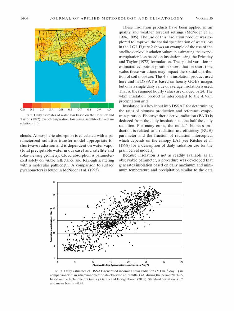
Because insolation is not as readily available as an

observable parameter, a procedure was developed that

generates insolation based on daily maximum and mini-

mum temperature and precipitation similar to the data

FIG. 2. Daily estimates of water loss based on the Priestley and

Taylor (1972) evapotranspiration loss using satellite-derived in-

solation (in.).

FIG. 3. Daily estimates of DSSAT-generated incoming solar radiation (MJ m22 day21) in

comparison with in situ pyranometer data observed at Camilla, GA, during the period 2003–05

based on the technique of Garcia y Garcia and Hoogenboom (2005). Standard deviation is 3.7

and mean bias is 20.45.

1464 J O U R N A L O F A P P L I E D M E T E O R O L O G Y A N D C L I M A T O L O G Y VOLUME 50

that are available for NWS Cooperative Observer Pro-

gram sites (Garcia y Garcia and Hoogenboom 2005;

Garcia y Garcia et al. 2008). While such a system makes

DSSAT easy to use at places where insolation data do not

exist, the generated data are not as desirable as direct

observations of insolation. With the advent of satellite

insolation products, the possibility exists to replace the

generated insolation with data that are observed by

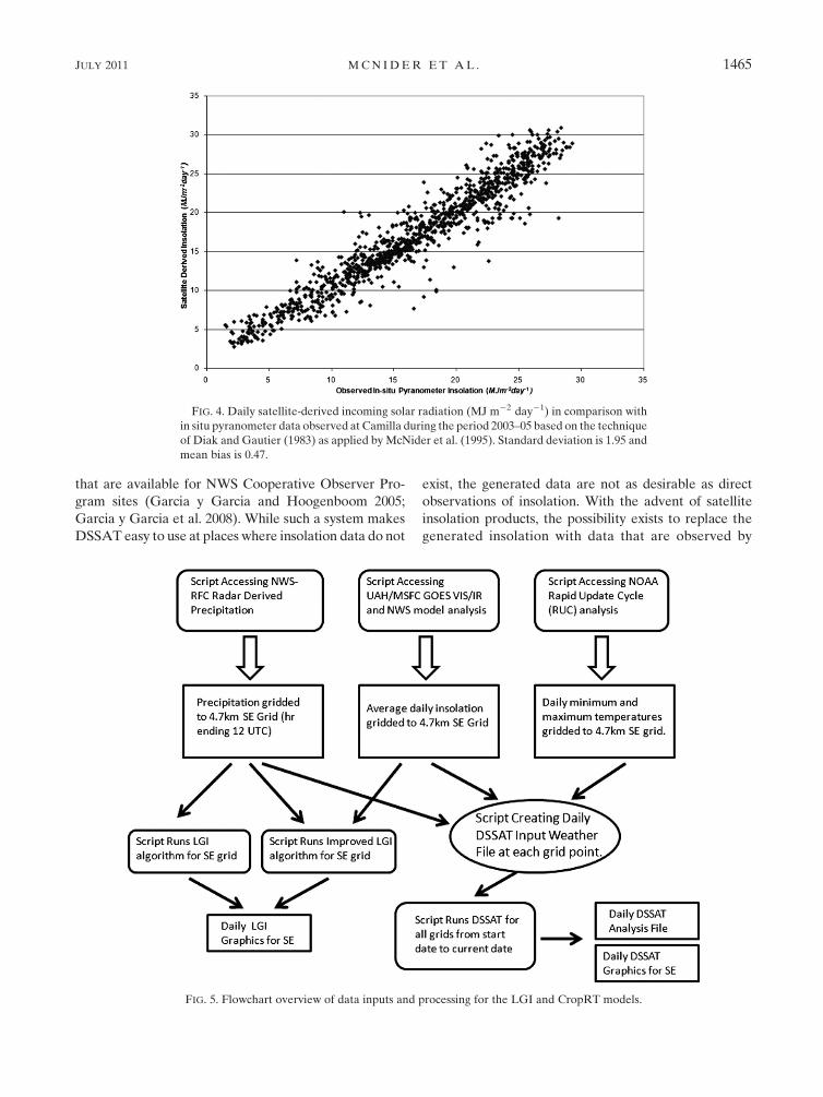
FIG. 4. Daily satellite-derived incoming solar radiation (MJ m22 day21) in comparison with

in situ pyranometer data observed at Camilla during the period 2003–05 based on the technique

of Diak and Gautier (1983) as applied by McNider et al. (1995). Standard deviation is 1.95 and

mean bias is 0.47.

FIG. 5. Flowchart overview of data inputs and processing for the LGI and CropRT models.

JULY 2011 M C N I D E R E T A L . 1465

satellites. Figures 3 and 4 show a comparison of gen-

erated data versus in situ data and of satellite insolation

compared with in situ data. Obviously, the space and

time attributes of the satellite allow for better agreement

than the generated data. However, in statistical tests

it was shown that the seasonal distribution (probabil-

ity density function, or PDF) of the generated insolation

compared favorably to the in situ PDF and to the satellite

data.

3. Gridded crop model system

The DSSAT system was configured to be run in a

gridded mode at a horizontal grid spacing of approxi-

mately 5 km. An input data file that defines the location

and soil type for each grid was developed. In this initial

testing, all soil parameters were set to be the same for

all grid points. Also, because of the data cutoff time of

1200 UTC in the operational system, the full dataset was

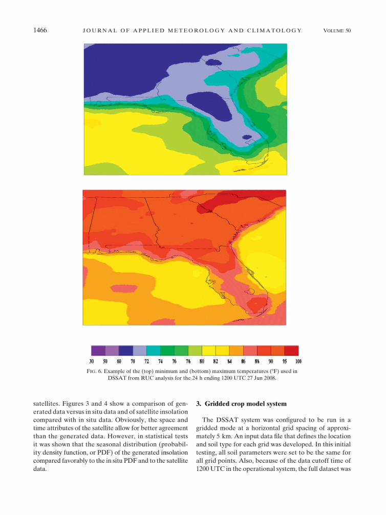
FIG. 6. Example of the (top) minimum and (bottom) maximum temperatures (8F) used in

DSSAT from RUC analysis for the 24 h ending 1200 UTC 27 Jun 2008.

1466 J O U R N A L O F A P P L I E D M E T E O R O L O G Y A N D C L I M A T O L O G Y VOLUME 50

not included in the model runs until the following day.

Thus, rainfall recorded after 1200 UTC was included in

the next day’s crop model run. The present system reflects

the water stress and yield impacts due only to meteo-

rology (i.e., the local weather conditions). The temporal

data required by DSSAT are daily minimum and max-

imum temperatures, daily insolation data, and daily pre-

cipitation data. All data were set to be run in real time

with scripts controlling the automatic acquisition of

temporal data. Figure 5 provides a flowchart schematic

of the CropRT and the LGI systems and their common

inputs.

a. Minimum and maximum temperature data

Minimum and maximum temperatures were taken

from the NOAA Rapid Update Cycle (RUC) analysis.

The RUC is a NOAA/National Centers for Environ-

mental Prediction (NCEP) operational weather pre-

diction system that includes a numerical forecast model

and an analysis–assimilation system (information online

at http://maps.fsl.noaa.gov). The current operational ver-

sion has a horizontal mesh size of about 13 km. The 2008

simulations were conducted using a horizontal mesh size

of about 40 km and it was run every hour. Minimum and

maximum temperatures were extracted for each model

grid point over a 24-h period ending at 1200 UTC from

the hourly RUC initialization analysis fields. These min-

imum and maximum temperatures were then interpo-

lated onto the grid that was used in the crop model (which

was the same grid as was used for the precipitation data,

4.7625 km). Figure 6 shows an example of the maxi-

mum and minimum temperatures as used in the DSSAT

gridded system.

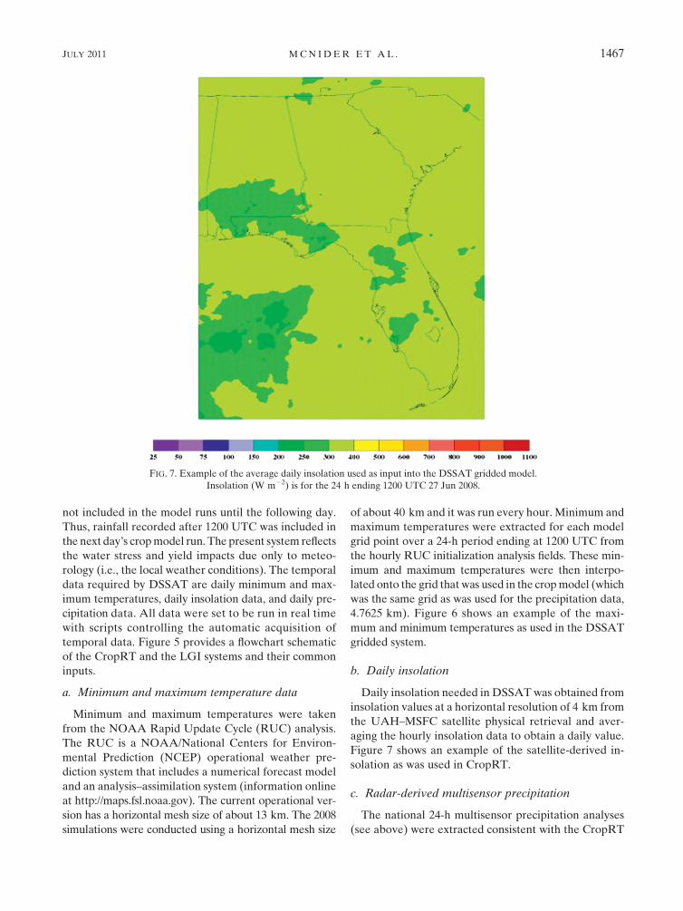
b. Daily insolation

Daily insolation needed in DSSAT was obtained from

insolation values at a horizontal resolution of 4 km from

the UAH–MSFC satellite physical retrieval and aver-

aging the hourly insolation data to obtain a daily value.

Figure 7 shows an example of the satellite-derived in-

solation as was used in CropRT.

c. Radar-derived multisensor precipitation

The national 24-h multisensor precipitation analyses

(see above) were extracted consistent with the CropRT

FIG. 7. Example of the average daily insolation used as input into the DSSAT gridded model.

Insolation (W m22) is for the 24 h ending 1200 UTC 27 Jun 2008.

JULY 2011 M C N I D E R E T A L . 1467

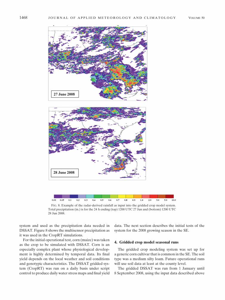
system and used as the precipitation data needed in

DSSAT. Figure 8 shows the multisensor precipitation as

it was used in the CropRT simulations.

For the initial operational test, corn (maize) was taken

as the crop to be simulated with DSSAT. Corn is an

especially complex plant whose physiological develop-

ment is highly determined by temporal data. Its final

yield depends on the local weather and soil conditions

and genotypic characteristics. The DSSAT gridded sys-

tem (CropRT) was run on a daily basis under script

control to produce daily water stress maps and final yield

data. The next section describes the initial tests of the

system for the 2008 growing season in the SE.

4. Gridded crop model seasonal runs

The gridded crop modeling system was set up for

a generic corn cultivar that is common in the SE. The soil

type was a medium silty loam. Future operational runs

will use soil data at least at the county level.

The gridded DSSAT was run from 1 January until

8 September 2008, using the input data described above

FIG. 8. Example of the radar-derived rainfall as input into the gridded crop model system.

Total precipitation (in.) is for the 24 h ending (top) 1200 UTC 27 Jun and (bottom) 1200 UTC

28 Jun 2008.

1468 J O U R N A L O F A P P L I E D M E T E O R O L O G Y A N D C L I M A T O L O G Y VOLUME 50

in and after the fact analysis (i.e., not in real time). The

planting date was made a function of latitude that ap-

proximates planting guidance from agricultural exten-

sion programs. It may not be robust in the subtropical

areas of Florida where soils are warm enough year round

to support germination. The planting date is given by

Planting day_of_year 5 (6:2 3 latitude) 2 126:

This formula yields day 60 at latitude 30 and day 91 at

latitude 35. Once the soil data have been added to the

system, these planting dates can be varied based on soil

color which, impacts soil warmup in the spring. In ad-

dition, actual temperatures from the temperature anal-

ysis might also be used to modify this. In the real-time

version, DSSAT is run to the current date using actual

observations; then, a forecast period to the predicted

final harvest date is conducted. At present this forecast

period is based on climatology, and improved forecast

strategies are under development. For example, future

versions might incorporate 10-day forecasts from NWP

products, then, using seasonal outlooks, go beyond 10

days. We do not report on any of the forecast data here

but only provide data driven by actual observations.

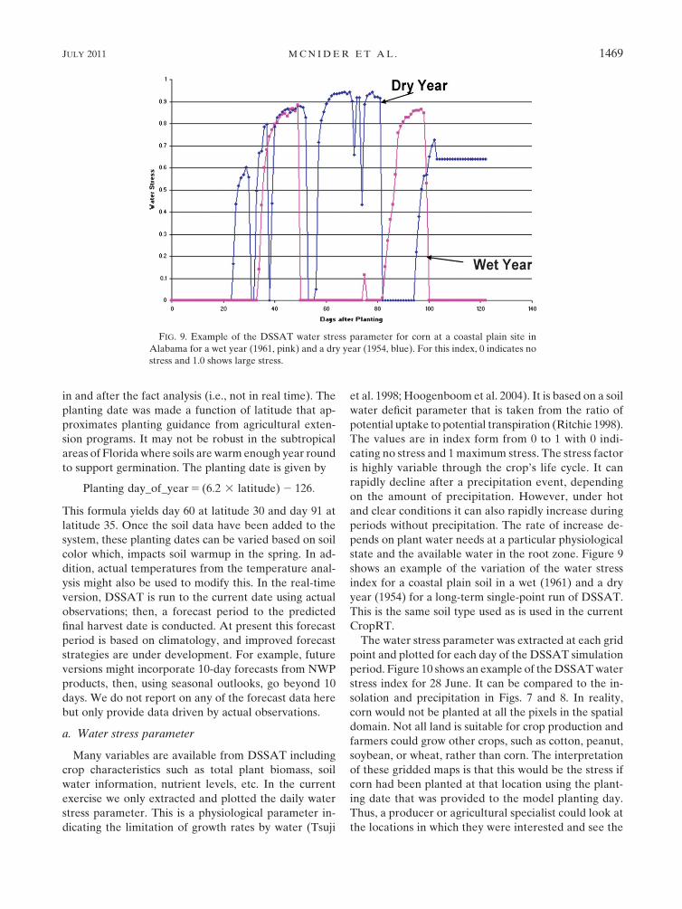
a. Water stress parameter

Many variables are available from DSSAT including

crop characteristics such as total plant biomass, soil

water information, nutrient levels, etc. In the current

exercise we only extracted and plotted the daily water

stress parameter. This is a physiological parameter in-

dicating the limitation of growth rates by water (Tsuji

et al. 1998; Hoogenboom et al. 2004). It is based on a soil

water deficit parameter that is taken from the ratio of

potential uptake to potential transpiration (Ritchie 1998).

The values are in index form from 0 to 1 with 0 indi-

cating no stress and 1 maximum stress. The stress factor

is highly variable through the crop’s life cycle. It can

rapidly decline after a precipitation event, depending

on the amount of precipitation. However, under hot

and clear conditions it can also rapidly increase during

periods without precipitation. The rate of increase de-

pends on plant water needs at a particular physiological

state and the available water in the root zone. Figure 9

shows an example of the variation of the water stress

index for a coastal plain soil in a wet (1961) and a dry

year (1954) for a long-term single-point run of DSSAT.

This is the same soil type used as is used in the current

CropRT.

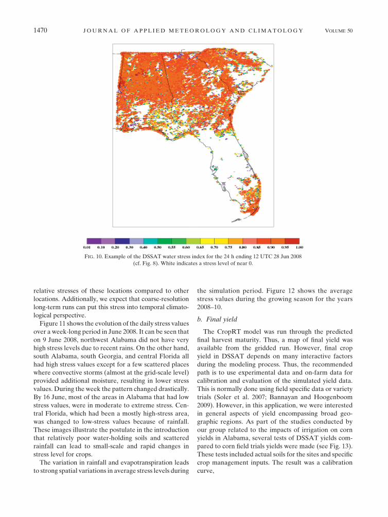
The water stress parameter was extracted at each grid

point and plotted for each day of the DSSAT simulation

period. Figure 10 shows an example of the DSSAT water

stress index for 28 June. It can be compared to the in-

solation and precipitation in Figs. 7 and 8. In reality,

corn would not be planted at all the pixels in the spatial

domain. Not all land is suitable for crop production and

farmers could grow other crops, such as cotton, peanut,

soybean, or wheat, rather than corn. The interpretation

of these gridded maps is that this would be the stress if

corn had been planted at that location using the plant-

ing date that was provided to the model planting day.

Thus, a producer or agricultural specialist could look at

the locations in which they were interested and see the

FIG. 9. Example of the DSSAT water stress parameter for corn at a coastal plain site in

Alabama for a wet year (1961, pink) and a dry year (1954, blue). For this index, 0 indicates no

stress and 1.0 shows large stress.

JULY 2011 M C N I D E R E T A L . 1469

relative stresses of these locations compared to other

locations. Additionally, we expect that coarse-resolution

long-term runs can put this stress into temporal climato-

logical perspective.

Figure 11 shows the evolution of the daily stress values

over a week-long period in June 2008. It can be seen that

on 9 June 2008, northwest Alabama did not have very

high stress levels due to recent rains. On the other hand,

south Alabama, south Georgia, and central Florida all

had high stress values except for a few scattered places

where convective storms (almost at the grid-scale level)

provided additional moisture, resulting in lower stress

values. During the week the pattern changed drastically.

By 16 June, most of the areas in Alabama that had low

stress values, were in moderate to extreme stress. Cen-

tral Florida, which had been a mostly high-stress area,

was changed to low-stress values because of rainfall.

These images illustrate the postulate in the introduction

that relatively poor water-holding soils and scattered

rainfall can lead to small-scale and rapid changes in

stress level for crops.

The variation in rainfall and evapotranspiration leads

to strong spatial variations in average stress levels during

the simulation period. Figure 12 shows the average

stress values during the growing season for the years

2008–10.

b. Final yield

The CropRT model was run through the predicted

final harvest maturity. Thus, a map of final yield was

available from the gridded run. However, final crop

yield in DSSAT depends on many interactive factors

during the modeling process. Thus, the recommended

path is to use experimental data and on-farm data for

calibration and evaluation of the simulated yield data.

This is normally done using field specific data or variety

trials (Soler et al. 2007; Bannayan and Hoogenboom

2009). However, in this application, we were interested

in general aspects of yield encompassing broad geo-

graphic regions. As part of the studies conducted by

our group related to the impacts of irrigation on corn

yields in Alabama, several tests of DSSAT yields com-

pared to corn field trials yields were made (see Fig. 13).

These tests included actual soils for the sites and specific

crop management inputs. The result was a calibration

curve,

FIG. 10. Example of the DSSAT water stress index for the 24 h ending 12 UTC 28 Jun 2008

(cf. Fig. 8). White indicates a stress level of near 0.

1470 J O U R N A L O F A P P L I E D M E T E O R O L O G Y A N D C L I M A T O L O G Y VOLUME 50

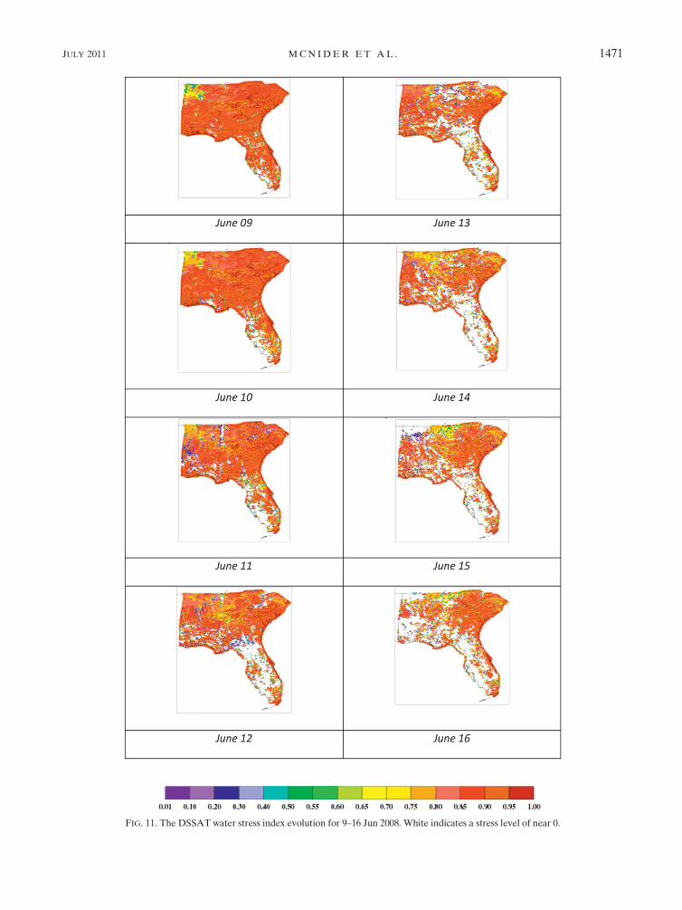
FIG. 11. The DSSAT water stress index evolution for 9–16 Jun 2008. White indicates a stress level of near 0.

JULY 2011 M C N I D E R E T A L . 1471

y 5 0:791x 1 35:147,

where x is the DSSAT yield and y is the adjusted yield in

units of bushels (bu) per acre. To make an independent

test of this relationship, the calibration was applied to

long-term (56 yr) DSSAT yields for three sites in Ala-

bama. The sites represented three major climatological

and soil regions and ranged from an Alabama coastal

plain to a prairie setting in the Blackbelt region in the

middle part of the state to the Tennessee Valley area in

northern Alabama. The three sites were averaged to

give a pseudostatewide average. This statewide average

was then compared to statewide yields from the USDA’s

National Agricultural Statistics Service (USDA/NASS).

The NASS data were detrended to mitigate systemic

increases in yields as a result of cultivar improvements

and agricultural practices through the 56-yr period. This

comparison is given in Fig. 14. While the average of the

three sites has a larger variance than the statewide

NASS data, the calibration appears to capture the year-

to-year patterns of variability in the NASS data. The

smaller variance in the NASS statewide numbers would

be expected since it is averaged using numerous differ-

ent weather conditions over many areas rather than just

three sites. The increase in variance in the NASS state-

wide data in recent years may be due to the drastic de-

crease in corn acreage in Alabama (from 2.5 million acres

in 1950 to 300 000 in 2006) and the concentration of corn

production in north Alabama.

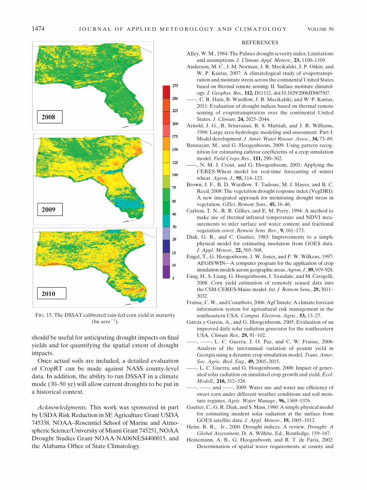
The calibration of crop model yields based on the

Alabama tests were applied to the gridded DSSAT runs

made for 2008–10. The calibrated yields for 3 yr are

given in Fig. 15. The Alabama-based calibration may not

be applicable to the other areas, especially Florida. The

blue areas of very low yields in southeast Georgia and in

south Florida are due to a failure to germinate that was

predicted by DSSAT due to inadequate soil moisture.

This picture is interesting in that it shows the estimated

variation in yields due to weather (temperature, in-

solation, and precipitation). The comparison of the yield

(Fig. 15) and average water stress (Fig. 12) is especially

noteworthy as it shows that the integrated model stress is

a good indicator of final model yield, although addi-

tional comparisons are needed against actual yields.

Thus, daily stress values (before crops reach maturity)

have some skill in projecting final yields. While DSSAT

water stress is tied to crop requirements and to canopy

area, the water stress may not give the full picture at

critical times in the plant’s life cycle. Concurrent maps of

water stress and plant stage, such as flowering, may be

better measures of impact on yield; therefore, this re-

lationship needs to be further analyzed (Garcia y Garcia

et al. 2009).

5. Summary and conclusions

This paper describes a first attempt to include rela-

tively high-resolution input data and plant physiological

behavior in a new type of spatial agricultural drought

index based on the stress level produced by a physiological-

based crop model. Multisensor high-resolution precipita-

tion products and high-resolution insolation products

were used in a gridded version of the DSSAT crop mod-

eling system. Corn was chosen as the specific crop. The

system was run for the 2008 and 2009 growing seasons in

FIG. 12. Average DSSAT water stress index during plant growth.

White indicates a stress level of near 0, which may occur if the crop

failed to germinate.

1472 J O U R N A L O F A P P L I E D M E T E O R O L O G Y A N D C L I M A T O L O G Y VOLUME 50

an after-the-fact analysis. The same system is currently

being evaluated for the real-time performance during the

2010 growing season.

The output from the model gives a map of daily water

stress that reflects a reduction in the potential growth

rate of corn and kernel development. End-of-year re-

sults provide a spatial estimate of corn yield. The results

indicate (as postulated in the introduction) that even in

years where large-scale drought is not present, signifi-

cant crop losses are present.

The current version reported here is a first-generation

system that only includes spatial variations in atmo-

spheric inputs. Future versions will include spatial var-

iations in soil types and profiles (Engel et al. 1997;

Heinemann et al. 2002). Additional work relating

DSSAT water stress to final yield is needed. The product

FIG. 13. Summary calibration chart from field trial data across three years 2000–03 and across

all geographic sites. The largest outlier (offline point) is from a wet year (2003).

FIG. 14. Application of calibration to DSSAT yields in comparison with Alabama statewide

NASS yields. DSSAT yields are an average of three sites in Alabama representing three major

soil and climatological regimes (bu acre21).

JULY 2011 M C N I D E R E T A L . 1473

should be useful for anticipating drought impacts on final

yields and for quantifying the spatial extent of drought

impacts.

Once actual soils are included, a detailed evaluation

of CropRT can be made against NASS county-level

data. In addition, the ability to run DSSAT in a climate

mode (30–50 yr) will allow current droughts to be put in

a historical context.

Acknowledgments. This work was sponsored in part

by USDA Risk Reduction in SE Agriculture Grant USDA

745338, NOAA–Rosenstiel School of Marine and Atmo-

spheric Science/University of Miami Grant 745251, NOAA

Drought Studies Grant NOAA-NA06NES4400015, and

the Alabama Office of State Climatology.

REFERENCES

Alley, W. M., 1984: The Palmer drought severity index: Limitations

and assumptions. J. Climate Appl. Meteor., 23, 1100–1109.

Anderson, M. C., J. M. Norman, J. R. Mecikalski, J. P. Otkin, and

W. P. Kustas, 2007: A climatological study of evapotranspi-

ration and moisture stress across the continental United States

based on thermal remote sensing: II. Surface moisture climatol-

ogy. J. Geophys. Res., 112, D11112, doi:10.1029/2006JD007507.

——, C. R. Hain, B. Wardlow, J. R. Mecikalski, and W. P. Kustas,

2011: Evaluation of drought indices based on thermal remote

sensing of evapotranspiration over the continental United

States. J. Climate, 24, 2025–2044.

Arnold, J. G., R. Srinivasan, R. S. Muttiah, and J. R. Williams,

1998: Large area hydrologic modeling and assessment. Part I:

Model development. J. Amer. Water Resour. Assoc., 34, 73–89.

Bannayan, M., and G. Hoogenboom, 2009: Using pattern recog-

nition for estimating cultivar coefficients of a crop simulation

model. Field Crops Res., 111, 290–302.

——, N. M. J. Crout, and G. Hoogenboom, 2003: Applying the

CERES-Wheat model for real-time forecasting of winter

wheat. Agron. J., 95, 114–125.

Brown, J. F., B. D. Wardlow, T. Tadesse, M. J. Hayes, and B. C.

Reed, 2008: The vegetation drought response index (VegDRI):

A new integrated approach for monitoring drought stress in

vegetation. GISci. Remote Sens., 45, 16–46.

Carlson, T. N., R. R. Gillies, and E. M. Perry, 1994: A method to

make use of thermal infrared temperature and NDVI mea-

surements to infer surface soil water content and fractional

vegetation cover. Remote Sens. Rev., 9, 161–173.

Diak, G. R., and C. Gautier, 1983: Improvements to a simple

physical model for estimating insolation from GOES data.

J. Appl. Meteor., 22, 505–508.

Engel, T., G. Hoogenboom, J. W. Jones, and P. W. Wilkens, 1997:

AEGIS/WIN—A computer program for the application of crop

simulation models across geographic areas. Agron. J., 89, 919–928.

Fang, H., S. Liang, G. Hoogenboom, J. Teasdale, and M. Cavigelli,

2008: Corn yield estimation of remotely sensed data into

the CSM-CERES-Maize model. Int. J. Remote Sens., 29, 3011–

3032.

Fraisse, C. W., and Coauthors, 2006: AgClimate: A climate forecast

information system for agricultural risk management in the

southeastern USA. Comput. Electron. Agric., 53, 13–27.

Garcia y Garcia, A., and G. Hoogenboom, 2005: Evaluation of an

improved daily solar radiation generator for the southeastern

USA. Climate Res., 29, 91–102.

——, ——, L. C. Guerra, J. O. Paz, and C. W. Fraisse, 2006:

Analysis of the interannual variation of peanut yield in

Georgia using a dynamic crop simulation model. Trans. Amer.

Soc. Agric. Biol. Eng., 49, 2005–2015.

——, L. C. Guerra, and G. Hoogenboom, 2008: Impact of gener-

ated solar radiation on simulated crop growth and yield. Ecol.

Modell., 210, 312–326.

——, ——, and ——, 2009: Water use and water use efficiency of

sweet corn under different weather conditions and soil mois-

ture regimes. Agric. Water Manage., 96, 1369–1376.

Gautier, C., G. R. Diak, and S. Mass, 1980: A simple physical model

for estimating incident solar radiation at the surface from

GOES satellite data. J. Appl. Meteor., 19, 1005–1012.

Heim, R. R., Jr., 2000: Drought indices: A review. Drought: A

Global Assessment, D. A. Wilhite, Ed., Routledge, 159–167.

Heinemann, A. B., G. Hoogenboom, and R. T. de Faria, 2002:

Determination of spatial water requirements at county and

FIG. 15. The DSSAT calibrated rain-fed corn yield at maturity

(bu acre21).

1474 J O U R N A L O F A P P L I E D M E T E O R O L O G Y A N D C L I M A T O L O G Y VOLUME 50

regional levels using crop models and GIS: An example for the

State of Parana. Agric. Water Manage., 52, 177–196.

Hoogenboom, G., 2000: Contribution of agrometeorology to the

simulation of crop production and its applications. Agric. For.

Meteor., 103, 137–157.

——, and Coauthors, 2004: Decision Support System for Agro-

technology Transfer, version 4.0. University of Hawaii, Hon-

olulu, HI, CD-ROM.

Jones, J. W., and Coauthors, 2003: DSSAT Cropping System

Model. Eur. J. Agron., 18, 235–265.

Keyantash, J., and J. A. Dracup, 2002: The quantification of

drought: An evaluation of drought indices. Bull. Amer. Me-

teor. Soc., 83, 1167–1180.

Kogan, F. N., 1995: Droughts of the late 1980s in the United States

as derived from NOAA polar-orbiting satellite data. Bull.

Amer. Meteor. Soc., 76, 655–668.

McNider, R. T., A. Song, D. M. Casey, P. J. Wetzel, W. L. Crosson,

and R. M. Rabin, 1994: Toward a dynamic–thermodynamic

assimilation of satellite surface temperature in numerical at-

mospheric models. Mon. Wea. Rev., 122, 2784–2803.

——, ——, and S. Q. Kidder, 1995: Assimilation of GOES-derived

solar insolation into a mesoscale model for studies of cloud

shading effects. Int. J. Remote Sens., 16, 2207–2231.

Narasimhan, B., and R. Srinivasan, 2005: Development and eval-

uation of soil moisture deficit index (SMDI) and evapotrans-

piration deficit index (ETDI) for agricultural drought

monitoring. Agric. For. Meteor., 133, 69–88.

Nemani, R. R., and S. W. Running, 1989: Estimation of regional

surface resistance to evapotranspiration from NDVI and

thermal-IR AVHRR Data. J. Appl. Meteor., 28, 276–284.

Niemeyer, S., 2008: New drought indices. First Int. Conf. on Drought

Management: Scientific and Technological Innovations, Zaragoza,

Spain, Joint Research Centre of the European Commission.

[Available online at http://www.iamz.ciheam.org/medroplan/

zaragoza2008/Sequia2008/Session3/S.Niemeyer.pdf.]

Norman, J. M., W. P. Kustas, and K. S. Humes, 1995: A two-source

approach for estimating soil and vegetation energy fluxes from

observations of directional radiometric surface temperatures.

Agric. For. Meteor., 77, 263–293.

Palmer, W. C., 1965: Meteorological drought. U.S. Weather Bu-

reau Res. Paper 45, 58 pp. [Available from NOAA Library

and Information Services Division, Washington, DC 20852.]

——, 1968: Keeping track of crop moisture conditions, nationwide:

The new crop moisture index. Weatherwise, 21, 156–161.

Paz, J. O., and Coauthors, 2007: Development of an ENSO-based

irrigation decision support tool for peanut production in the

southeastern US. Comput. Electron. Agric., 55, 28–35.

Pinker, R. T., and Coauthors, 2003: Surface radiation budgets

in support of the GEWEX Continental-Scale International

Project (GCIP) and the GEWEX Americas Prediction Project

(GAPP), including the North American Land Data Assimi-

lation System (NLDAS) Project. J. Geophys. Res., 108, 8844,

doi:10.1029/2002JD003301.

Pour-Biazar, A., and Coauthors, 2007: Correcting photolysis rates

on the basis of satellite observed clouds. J. Geophys. Res., 112,

D10302, doi:10.1029/2006JD007422.

Priestley, C. H., and R. J. Taylor, 1972: On the assessment of sur-

face heat flux and evaporation using large scale parameters.

Mon. Wea. Rev., 100, 81–92.

Ritchie, J. T., 1972: Model for predicting evaporation from a row-

crop with incomplete cover. Water Resour. Res., 8, 1204–1213.

——, 1998: Soil water balance and plant water stress. Un-

derstanding Options for Agricultural Production, G. Y. Tsuji,

G. Hoogenboom, and P. K. Thornton, Eds., Systems Ap-

proaches for Sustainable Agricultural Development, Vol. 7,

Kluwer Academic, 42–54.

——, U. Singh, D. Godwin, and W. Bowen, 1998: Cereal growth,

development and yield. Understanding Options for Agricultural

Production, G. Y. Tsuji, G. Hoogenboom, and P. K. Thornton,

Eds., Systems Approaches for Sustainable Agricultural De-

velopment, Vol. 7, Kluwer Academic, 79–98.

Sellers, P. J., 1985: Canopy reflectance, photosynthesis, and tran-

spiration. Int. J. Remote Sens., 6, 1335–1372.

Senay, G. B., 2008: Modeling landscape evapotranspiration by in-

tegrating land surface phenology and a water balance algo-

rithm. Algorithms, 1, 52–68, doi:10.3390/a1020052.

Soler, C. M. T., P. C. Sentelhas, and G. Hoogenboom, 2007: Ap-

plication of the CSM-CERES-Maize model for planting date

evaluation and yield forecasting for maize grown off-season in

a subtropical environment. Eur. J. Agron., 27, 165–177.

Svoboda, M., and Coauthors, 2002: The Drought Monitor. Bull.

Amer. Meteor. Soc., 83, 1181–1190.

Tarpley, J. D., 1979: Estimating incident solar radiation at the

surface from geostationary satellite data. J. Appl. Meteor., 18,

1172–1181.

Thornton, P. K., and G. Hoogenboom, 1994: A computer program

to analyze single-season crop model outputs. Agron. J., 86,

860–868.

Tsuji, G. Y., G. Hoogenboom, and P. K. Thornton, Eds., 1998:

Understanding Options for Agricultural Production, Sys-

tems Approaches for Sustainable Agricultural Development,

Vol. 7, Kluwer Academic, 400 pp.

Wetzel, P. J., 1984: Determining soil moisture from geosynchronous

satellite infrared data: A feasibility study. J. Climate Appl.

Meteor., 23, 375–391.

Wilhite, D. A., and M. H. Glantz, 1985: Understanding the

drought phenomenon: The role of definitions. Water Int., 10,

111–120.

JULY 2011 M C N I D E R E T A L . 1475

Copyright of Journal of Applied Meteorology & Climatology is the property of American Meteorological

Society and its content may not be copied or emailed to multiple sites or posted to a listserv without the

copyright holder's express written permission. However, users may print, download, or email articles for

individual use.