A Rapidly Mixing Monte Carlo Method for the Simulation of Slow Molecular Processes

0

A rapidly Mixing Monte Carlo Method for the

Simulation of Slow Molecular Processes

V. Durmaz, K. Fackeldey, M. WeberZuse Institute Berlin

Germany

1. Introduction

Since the middle of the last century, the continously increasing computational power hasbeen adopted to molecular modeling and the simulation of molecular dynamics as well. Inthis field of research, one is interested in the dynamical behaviour of molecular systems.In contrast to the beginnings when only single or very few atoms could be simulated,the systems under consideration have grown to the size of macromolecules like proteins,DNA, or membrane structures nowadays resulting in high-dimensional conformationalspaces. This development is triggered by permanently increasing computational power, theutilization of massively parallel hardware as well as improved algorithms and enhancedmolecular force fields, covering chemical and especially biological molecular systems ata progressive rate. Applications basing on molecular modeling help to understand andpredict molecular phenomena in various fields of applications providing information on e. g.molecular conformations and recognition, protein folding, drug-design, or binding affinities.Typical fields benefiting from their usage are pharmacy, medicine, chemistry and materialsresearch.Unfortunately, often the atomistic structure is so complex that a satisfactory mapping of theprocesses can hardly be realized, due to the large number of atoms and in particular, thedifference in time scales. More precisely, for the molecular function of a protein for example,its folding is a key issue. In contrast to this folding event that may last up to several secondsor even minutes, the time step of an ordinary trajectory based molecular simulation is linkedto the fastest molecular oscillation which occurs in case of the chemical H − C bond with atime period around few 10−15 seconds. Even today, exorbitant computational effort and timeneed to be invested in order to capture such interesting processes.

2. Atomistic simulations

The molecular simulation methods can be divided into two classes: the deterministic andthe stochastic approaches. The first one is also known as the classical molecular dynamcis(MD), which relies on classical mechanics as described by Newton’s Equations of motion(e.g. Frenkel & Smit (1996); Griebel et al. (2007)). The latter class is known as Monte CarloMethods (e.g. Binder & Landau (2000)). Both methods have celebrated a great success invarious applications. For an overview, we refer to Leach (2001) and Schlick (2002).

22

www.intechopen.com

In the forthcoming we will briefly introdcue the molecular dynamics and then give a moredetailed introdcution into the Monte Carlo method within its framework. Later on, we willeploit the commonalities between both simulation methods in order to explain the hybridMonte Carlo method.

2.1 Deterministic molecular simulations

The basic idea of molecular dynamics is to calculate trajectories containing spatial coordinatesof atoms evolved in time. Let us assume, a state x = (q, p) ∈ R

6n of a molecular system withn atoms is given in a 6n-dimensional phase space. Here, q ∈ Ω ⊂ R

3n and p ∈ Γ ⊂ R3n

denote the position coordinates in the position space Ω and the momentum cooridnates inthe momentum space Γ, respectively. For a classical description of molecular motion withconservative forces, Newton’s second law is given by the equation

Mq = f (q),

where M ∈ R3n×3n is a diagonal matrix of atomic masses, f (q) ∈ R

3n is a vector of internaland external forces acting on the atoms at position q, and q stands for the acceleration asthe second time derivative of q. The total energy of the system under consideration, i.e. theHamiltonian H is given by

H(p, q) = V(q) + K(p), (1)

where K(p) = 12 p

TM−1p and V(q) represent the kinetic and the poteintial part, respectively.Since the kinetic part only depends on the momenta and the potential part on the positionsonly, the Hamiltonian is separable, leading to the following equations of motion:

q =∂H (p, q)

∂p=

∂K (p)

∂p= M−1p (2a)

p =∂H (p, q)

∂q=

∂V (q)

∂q= −∇qV(q) . (2b)

Inserting these two time derivatives q and p into the time derivative of the Hamiltonian

dH (p, q)

dt=

(∇qH

)︸︷︷︸

=− p

q +(∇pH

)︸︷︷︸

=q

p = − pq + pq = 0 (3)

shows that the total energy according to Hamilton is constant over time, i. e. H(q(t), q(t)) =H(q(0), q(0)) for t ∈ (−∞, ∞). Time discretization during simulation is achieved by applyinga constant step size integrator like the Sörmer-Verlet (Verlet (1967)) or leap-frog (Hockney(1970)) integrator for which the time step size Δt is determined by the shortest oscillationperiod of bonds in a molecule, namely some femtoseconds. In addition, a time integrationfor a sampling scheme as represented by Equation (2) has to fulfil certain properties likereversibility and symplecticity. Besides the fact that the time step is confined to a small size,the total time span τ, i.e. the time of the simulation, has to be chosen carefully as well. Moreprecisely, for a given initial state x(0) and a slightly perturbated state x∗(0) it can be shown:

‖x(t) − x∗(t)‖ ∼ ‖x(0) − x∗(0)‖ exp(λmaxt)

which means that the error ‖x(t) − x∗(t)‖ depends exponentially on the time, where λmax

is the maximal Lyapunov characteristic exponent. It has been shown by Deuflhard et al.

400 Applications of Monte Carlo Methods in Biology, Medicine and Other Fields of Science

www.intechopen.com

(1999), that for molecular dynamics λmax may be very large such that only trajectories of some10−13 seconds are correlated with the initial state. Due to the large λmax value, moleculardynamics is chaotic. However, if one is interested in the probability of rare events during thischaotic process, e. g. protein folding, the deterministic trajectory based approach seems notfavourable. Here, we do not focus on these aspects and refer to Leimkuhler & Reich (2004) fordetails.Having briefly scetched the idea of the classical molecular dynamics, we now change ourpoint of view to the concept of statistical dynamics and investigate ensembles of molecularsystems.

2.2 Statistical molecular simulations

In statistical molecular dynamcis, we are not interested in the movement or speed of eachparticle but in averaged macroscopic properties of the atoms. The advantage of this approachlies in the fact that many physical properties in which we are interested, like energies,enthalpies and entropies do not depend strongly on a detailed dynamical movement of eachparticle but on a collection of particles. In other words, we are no longer interested in eachparticle but in a system of particles and its probability to be in a certain state. In order todescribe this state, we need the term “ensemble” which is an imaginary collection of systemsdescribed by the same Hamiltonian where each system is in a unique mircoscopic state at anygiven instant time.In an (n,V, T)-ensemble, each subsystem, in our example of section 4 it is a single moleculein vacuum, has the same macroscopic properties volume V and temperature T. Furthermore,neither chemical reactions take place nor do particles escape which means that the numbern of atoms is also kept constant. The subsystems can only exchange energy with theirsurroundings and therefore, have different states x = (q, p) to which Boltzmann statisticscan be applied. For a detailed derivation of the Boltzmann distribution which is defined asthe most probable distribution of states in an (n,V, T)-ensemble and is also called canonicalensemble μcan, see Schäfer (1960), pp. 5–11. Via the Hamiltonian H(·), the probability that amolecule attains the state x is

μcan(x) =1

Zexp(−β H(x)),

where Z is a corresponding normalization. β is the inverse temperature

β =1

kBT,

where T is measured in Kelvin and kB ≈ 1.38066 · 10−23 J K−1 is the Boltzmann constant.

2.2.1 Partition functions

For separable Hamiltonian functions, the Boltzmann distribution of molecular states x =(q, p) in the canonical ensemble μcan(x) = π(q)η(p) has the following splitting into adistribution of momenta and position states:

η(p) =1

Zpexp(−βK(p)), π(q) =

1

Zqexp(−βV(q)).

η(·) represents a Gaussian distribution for each of the 3n momenta coordinates, because K isa quadratic function with the diagonal matrix M.

401A rapidly Mixing Monte Carlo Method for the Simulation of Slow Molecular Processes

www.intechopen.com

Therefore, creating a sequence of momenta numerically (sampling) according to theirBoltzmann distribution η(p) is simple, see e.g. Allen & Tildesley (1987). The spacial factor π(·)is a more complex distribution function. Whereas the exponential function exp(−βV(q)) canbe computed pointwise, the normalization constant (also denoted as spatial partition function1)

Zq =∫

Ωexp(−βV(q)) dq (4)

is unknown. For a sampling of points q ∈ Ω according to a distribution which is known exceptfor a normalization constant, the Metropolis-Hastings algorithm can be applied, see section 3.

2.2.2 Bracket notation

A macroscopic measurement is always carried out for a snapshot of a molecular ensemble,where molecular states are distributed according to the Boltzmann distribution. A spatialobservable 〈A〉π of a function A : Ω → R in configuration space, e. g. potential energiesor torsion angles, is therefore measured as an ensemble mean, i. e. an expectation value

〈A〉π =∫

ΩA(q) π(q) dq, (5)

where A is μ-Lebesgue integrable w. r. t. the measure μ(dq) := π(q) dq. In the following, thesebracket notations for observable and inner products will be often used abbreviations.

2.2.3 Importance sampling

In Equation 5 the dimension of the space Ω is proportional to the number of degrees offreedom. The evaluation of this integral leads to a high-dimensional numerical integrationproblem. Thus, a regular or equidistant grid in the phase space combined with a standarddeterministic integration scheme, such as Simpsons rule cannot be used (see Table 1).

Method Convergene

Trapeziodal N−2/d

Simpson N−4/d

Monte Carlo N−1/2

Table 1. The convergence behaviour of the determinstic quadrature rules (Simpson andTrapezoidal) depend on the dimension: With increasing number of dimension, theconvergence rate growth. In contrast, the convergence behavior of the Monte Carlo methoddoes not depend on the dimension

In a Monte Carlo method one solves numerically

∫

Ωg(x)dx ≈

1

N

N

∑i=1

g(xi).

The key issue in a Monte Carlo method, is that the evaluation points x1, ..., xN are statisticallyselected. There are many ways how to distribute the points. If they are distributed uniformly,it is called a simple sampling.

1 Zq is a function of temperature, volume and number of particles of an ensemble. For the canonicalensemble Zq is a constant. The total partition function Z = ZqZp is the key to calculating all macroscopicproperties of the system.


www.intechopen.com

However, for complex functions like π (q), a simple sampling is inappropriate since theuniform distribution of particles might lead to an insufficient reproduction of the function(see center distribution of Fig. 1). Fig. 1 illustrates well that it is not easy to generate a gooddistribution of particles in a reasonable amount of computer time. In the importance sampling,the integrand is modified in order to yield an expectation of a quantity that varies less than theoriginal integrand over the region of integration. In order to solve Equation (5), one appliesMonte Carlo integration methods with an importance sampling routine, i.e.

〈A〉π ≈1

N

N

∑i=1

A(qi), qi ∝ π, (6)

where N position states qi ∈ Ω are sampled according to their Boltzmann distribution π.Hence, the expectation value of an observable can be simply approximated by its arithmeticmean. For introductory literature of Monte Carlo integration methods see Hammersley &Handscomb (1964) and Robert & Casella (1999).Since the major part of the conformational space Ω is physically irrelevant due to highpotential energies V (q), only few conformations have a probability substantially larger thanzero. Instead of creating independent points qi, in practice, one starts with a physicallyrelevant position state q1 ∈ Ω and generates further states via a Markov chain

q1 → q2 → . . . → qN . (7)

Summing up, both approaches have advantages and disadvantages. In classicalmolecular dynamics simulations the motion of each individual particle can be describeddeterministically. However, long simulations are hardly feasible. On the other hand, thestatistical molecular simulation is capable of handling large molecular systems but lacks of atrajectory.

Fig. 1. Left: A simple sampling with a uniformly distributed set of particles fitting a nearlyconstant function. Center: A simple sampling inappropriate for unconstant distributionfunctions. Right: A suitable distribution of points well fitting the desired function(importance sampling).

3. Hybrid Monte Carlo method (HMC)

The conclusion of the forgoing section is a motivation to construct a method which profitsfrom either of the two approaches. This has been done in the hybrid Monte Carlo method.Roughly speaking, this method can be seen as a combination of deterministic moleculardynamics combined with stochastic impulses. So far we have elucidated the basic frameworkof statistical simulations but not their numerical realization in detail. This will be done in thenext prargraphs.


www.intechopen.com

3.1 Detailed balance criterion

A sufficient condition for a correct sampling via Monte Carlo Simulation in the situation ofEquation 7 is the detailed balance condition with the desired Boltzmann distribution π. Thiscondition holds, if the conditional probability density function P(q → q) for a transition q → qin Equation 7 meets

π(q) P(q → q) = π(q) P(q → q) (8)

where the occurrence of a certain position state q in 7 is proportional to te probability π(q).Equation 8 describes the thermodynamic equilibrium of a molecular system with two (ormore) possible states/conformations q and q. The probability of being in state q and switchingover to state q is equal to the probability for the reverse way. For the sufficient and necessary“balance condition” which is less rigorous than Equation 8, see Manousiouthakis & Deem(1999).

3.2 Metropolis-Hastings algorithm

In the following, we use a Metropolis-Hastings type algorithm (Metropolis et al. (1953)) wherethe transition probability density function P in Equation 8 is split into two factors

P(q → q) = Ppr(q → q) Pac(q → q). (9)

Here is the corresponding sampling scheme:

• In Equation 9, Ppr is a proposal probability density function, i.e. the probability that afterq ∈ Ω a position state q ∈ Ω is proposed as candidate for the next step in the Markov chain(see Equation 7).

• With an acceptance probability of Pac, the next step in the chain is q, with a probability of1 − Pac the step q is repeated in Equation 7. For a numerical realization of the acceptanceprobability, one computes a uniformly distributed random number r ∈ [0, 1] and accepts qif r ≤ Pac(q → q).

With Equation 8 a sufficient condition for a correct sampling according to this scheme is:

π(q) Ppr(q → q) Pac(q → q) = π(q) Ppr(q → q) Pac(q → q).

For a given (ergodic) proposal probability density function Ppr, a possible choice for Pac

satisfying the latter equation is for example the Metropolis dynamics:

Pac(q → q) = min{

1,π(q) Ppr(q → q)

π(q) Ppr(q → q)

}. (10)

Metropolis dynamics provides a chain of the form of Equation 9 with minimal asymptoticvariance and is therefore the most popular one (see Peskun’s theorem in Peskun (1973)).

3.3 Combination of MCMC and MD.

The transition probabilities P(q → q) doesn’t need to have any physical meaning in order tomeet Equation 8, but for a good acceptance ratio Pac, a combination of the Metropolis-Hastingsalgorithm for Markov chain Monte Carlo integration (MCMC) with molecular dynamicssimulations (MD) is useful.Starting in 1980, a variety of hybrid methods have been developed, which take the advantagesof both MD and MCMC (Andersen (1980); Duane et al. (1987)). These so-called HMCalgorithms where originally developed for quantum chromo-dynamics, but they have been


www.intechopen.com

used successfully for condensed-matter systems (Clamp et al. (1994); Forrest & Suter (1994);Gromov & de Pablo (1995); Irbäck (1994); Mehlig et al. (1992)) and also for biomolecularsimulations (Fischer et al. (1998); Hansmann et al. (1996); Zhang (1999)). HMC combinesthe large steps of MD in phase space with the property of MCMC to ensure ergodicity byaltering orbits in phase space and to eliminate inaccuracies in the numerical computationof the Hamiltonian dynamics. In the following the HMC method is explained according toFischer (1997).

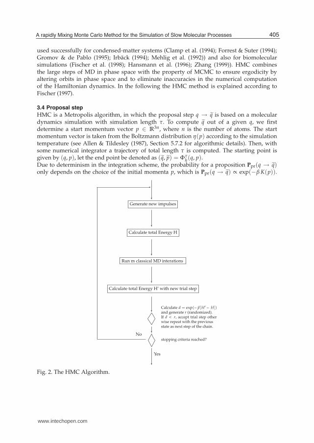
3.4 Proposal step

HMC is a Metropolis algorithm, in which the proposal step q → q is based on a moleculardynamics simulation with simulation length τ. To compute q out of a given q, we firstdetermine a start momentum vector p ∈ R

3n, where n is the number of atoms. The startmomentum vector is taken from the Boltzmann distribution η(p) according to the simulationtemperature (see Allen & Tildesley (1987), Section 5.7.2 for algorithmic details). Then, withsome numerical integrator a trajectory of total length τ is computed. The starting point isgiven by (q, p), let the end point be denoted as (q, p) = Φτ

h(q, p).Due to determinism in the integration scheme, the probability for a proposition Ppr(q → q)only depends on the choice of the initial momenta p, which is Ppr(q → q) ∝ exp(−βK(p)).

Generate new impulses

Calculate total Energy H

Run m classical MD interations

Calculate total Energy H’ with new trial step

Calculate d = exp(− β[H − H])and generate r (randomized).If d < r, accept trial step other-wise repeat with the previousstate as next step of the chain.

Yes

Nostopping criteria reached?

Fig. 2. The HMC Algorithm.


www.intechopen.com

If the numerical integrator is momentum-reversible, then for the reverse step q → q, we haveto choose the start momentum vector − p, which transfers the starting point (q,− p) to (q,−p)in time span τ. This means, Ppr(q → q) ∝ exp(−βK(− p)). In Equation 8, the two terms areintegrated over the Lebesgue measure dq ∧ dq. After transformation into the momenta space,the left hand side depends on dq ∧ dp and the right had side on dq ∧ dp. But this does notchange anything in Equation 10 because the mapping (q, p) = Φτ

h(q, p) is area preserving.Both measures are equivalent. Inserting these results into 10 yields

Pac(q → q) = min{

1,π(q) exp(−βK(− p))

π(q) exp(−βK(p))

}

= min{

1,exp(−βV(q)) exp(−βK( p))

exp(−βV(q)) exp(−βK(p))

}

= min{

1, exp(−β (H(q, p) − H(q, p)))}

, (11)

i.e. the acceptance probability of the HMC proposal step is based on the change of the totalenergy during a numerical integration of the Hamiltonian. A reversible and area-preservingnumerical integrator is necessary and sufficient for a correct sampling. For a rigorous proof,see also Mehlig et al. (1992), Section III.

3.5 Choice of the numerical integrator

Table 2 shows some algorithmic details of HMC and related methods. It shows, whichHamiltonian the methods are based upon, the acceptance probabilities and eventually anecessary pointwise re-weighting of the sampling trajectory in order to be mathematicallyrigorous.

3.5.1 “Exact” flow

As we have seen in the derivation of the acceptance probability, a reversible andarea-preserving numerical integrator is necessary and sufficient for a correct sampling,no matter how bad its state space solution is. However, if we could apply an “exact”integrator the total energy would be constant during simulation, and therefore, the acceptanceprobability according to Metropolis dynamics would be 1. Adaptive integrators can be usedwith a pre-defined deviation from the exact flow. An example for an adaptive integrator forHamiltonian dynamics is DIFEX2, an extrapolation method based on Störmer discretization,see Deuflhard (1983) and Deuflhard (1985). For DIFEX2, area-preservation and reversibilitycannot be shown directly, but as the extrapolation method approximates the real flow, itinherits these properties from Φτ. Other adaptive integration methods and Fortran codes canbe found in the book of Hairer et al. (1993). See also the first row of Table 2.

Hamiltonian accept re-weight

“exact” flow H 1 no

orig. HMC H e−β ΔH< 1 no

SHMC (idea) H 1 H → H

SHMC Happ e−β ΔHapp ≈ 1 Happ → H

Table 2. Possible approaches for a correct sampling according to the HMC method.Algorithmic consequences.


www.intechopen.com

3.5.2 Original HMC

Instead of solving the real dynamics, one can apply an arbitrary area-preserving and reversibleintegrator. In this case, the mean acceptance ratio decreases exponentially with system size nand the time step discretization h in the numerical integration Φτ

h . See Gupta et al. (1990)and Kennedy & Pendleton (1991) for an analytic study of the computational cost of HMC. Itis a general opinion that HMC methods are only suitable for small molecular systems (seee.g. Section 14.2 in Frenkel & Smit (2002)). The reason is that in order to keep the meanacceptance probability constant for increasing system size, the time step h of the symplecticintegrator has to decrease accordingly. Instead of time step refinements, one can also increasethe order of the integration method. Using Hamilton’s principle of a stationary action integral,Wendlandt & Marsden (1997) derived a systematical scheme for creating so-called variationalintegrators. With these higher-order numerical integrators the acceptance ratio of HMC canbe improved due to better approximation properties. By omitting the constant step size hin variational integrators, one can even get symplectic and energy preserving integrationschemes for the price of lower numerical efficiency. For an excellent overview of thesemethods, see Lew et al. (2004). See also the second row of Table 2.

3.5.3 Shadow HMC (SHMC)

Another approach uses the fact that some symplectic numerical integrator solves the

dynamics of a modified Hamiltonian H exactly (see Hairer et al. (2004) or Skeel & Hardy(2002)). If one accepts each proposal step of the numerical dynamics simulation, this is likecomputing the density of the modified Hamiltonian (see third row of Table 2). In order to getthe right distribution in configuration space, one has to re-weight the resulting position states

accordingly. This is only possible, if the modified Hamiltonian is known. Fortunately, H canbe approximated up to arbitrary accuracy. For algorithmic details, see Izaguirre & Hampton(2004).

3.5.4 Approximated SHMC

Approximating the modified Hamiltonian as exactly as possible, is numerically expensive.

Therefore, one would like to truncate the Taylor expansion of H after a finite number of

terms in order to yield Happ. This method is part of the TSHMC method of Akhmatskaya &Reich (2004). Again, an acceptance rule is introduced which zeroes out the numerical errorof truncation (see the last row of Table 2). This method seems to be very promising forlarger molecules, because the acceptance probability is almost 1, the method is mathematically

rigorous and numerically efficient (extra cost for computation of Happ is negligible).

4. Example: Brominated flame retardant hexabromocyclododecane

1,2,5,6,9,10-Hexabromocyclododecane (HBCD) is a widely used additive brominated flameretardant (BFR) to plastic materials as upholstery textiles, styrene-acrylonitrile resins orpolystyrene foams (EPS, XPS) for the building sector with fractional percentages varyingbetween 0.8 and 4% (Barda et al. (1985); de Witt (2002); Janak et al. (2005)). In the face ofa world market demand of about 22000 metric tons in the year 2003 (Köppen et al. (2008)),HBCD is among a the most popular BFRs, especially in Europe (Janak et al. (2005)).However, it is regarded as a persistent organic pollutant (POP) and has been detectedincreasingly in the environment during the last decades, e. g. in sewage sludges and sediments(see de Wit et al. (2006); Hale et al. (2006); Vos et al. (2003)) as well as in diverse tissues of both


www.intechopen.com

terrestric and aquatic organisms (Janak et al. (2005); Tomy et al. (2004)). Even in the lipid phaseof human breast milk of women from diverse european countries and the USA traces of HBCDand other BFR have been detected (Covaci et al. (2006); Johnson-Restrepo et al. (2008)).

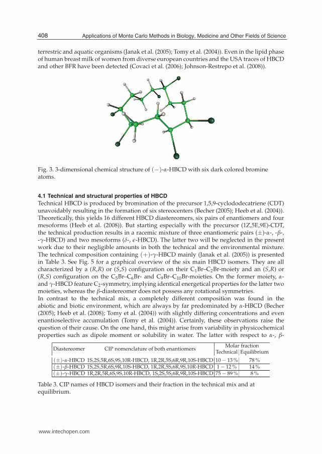
Fig. 3. 3-dimensional chemical structure of (−)-α-HBCD with six dark colored bromineatoms.

4.1 Technical and structural properties of HBCD

Technical HBCD is produced by bromination of the precursor 1,5,9-cyclododecatriene (CDT)unavoidably resulting in the formation of six stereocenters (Becher (2005); Heeb et al. (2004)).Theoretically, this yields 16 different HBCD diastereomers, six pairs of enantiomers and fourmesoforms (Heeb et al. (2008)). But starting especially with the precursor (1Z,5E,9E)-CDT,the technical production results in a racemic mixture of three enantiomeric pairs (±)-α-, -β-,-γ-HBCD) and two mesoforms (δ-, ǫ-HBCD). The latter two will be neglected in the presentwork due to their negligible amounts in both the technical and the environmental mixture.The technical composition containing (+)-γ-HBCD mainly (Janak et al. (2005)) is presentedin Table 3. See Fig. 5 for a graphical overview of the six main HBCD isomers. They are allcharacterized by a (R,R) or (S,S) configuration on their C1Br–C2Br-moiety and an (S,R) or(R,S) configuration on the C5Br–C6Br- and C9Br–C10Br-moieties. On the former moiety, α-and γ-HBCD feature C2-symmetry, implying identical energetical properties for the latter twomoieties, whereas the β-diastereomer does not possess any rotational symmetries.In contrast to the technical mix, a completely different composition was found in theabiotic and biotic environment, which are always by far predominated by α-HBCD (Becher(2005); Heeb et al. (2008); Tomy et al. (2004)) with slightly differing concentrations and evenenantioselective accumulation (Tomy et al. (2004)). Certainly, these observations raise thequestion of their cause. On the one hand, this might arise from variability in physicochemicalproperties such as dipole moment or solubility in water. The latter with respect to α-, β-

Diastereomer CIP nomenclature of both enantiomersMolar fraction

Technical Equilibrium

(±)-α-HBCD 1S,2S,5R,6S,9S,10R-HBCD, 1R,2R,5S,6R,9R,10S-HBCD 10 − 13 % 78 %(±)-β-HBCD 1S,2S,5R,6S,9R,10S-HBCD, 1R,2R,5S,6R,9S,10R-HBCD 1 − 12 % 14 %(±)-γ-HBCD 1R,2R,5R,6S,9S,10R-HBCD, 1S,2S,5S,6R,9R,10S-HBCD 75 − 89 % 8 %

Table 3. CIP names of HBCD isomers and their fraction in the technical mix and atequilibrium.


www.intechopen.com

Fig. 4. Cyclic-concerted interconversion mechanism. A necessary condition for thequantum-chemically induced process is the anti positioning of two vicinal bromine atomswhich leads to double-bonded bromines and five-bonded carbons during transition (centerstructure) caused by a nucleophilic attack of bromine. The interconversion results in a changeof the involved chiralities.

and γ-HBCD is relatively low and was measured to be 48.8, 14.7, and 2.1 μg/L, respectively(Hunziker et al. (2004)).On the other hand, differing diastereomeric ratios might be triggered by stereoselectiveuptake and metabolism. Indeed, there seems to be strong evidence for a biologically inducedinterconversion of HBCD stereoisomers (Hamers et al. (2006); Law et al. (2006a)). According toVos et al. (2003), Hamers et al. (2006), and Meerts et al. (2000), some BFRs such as HBCD or itsmetabolite pentabromocyclododecaene (PBCD) are suspected to cause endocrine disruption

Fig. 5. Graphical overview of all possible interconversions between any connected two of thesix main HBCD diastereomers taken from Köppen et al. (2008). The bromine anticonformation of any CiBr–Ci+1Br-moiety of the starting diastereomers triggers the inversionto another diastereomer depending on the couple of concerned bromine atoms, i. e.depending on the value of index i with i ∈ {1, 5, 9}. This transition process with rate kx→y isdenoted as cyclic-concerted interconversion.


www.intechopen.com

due to competition with thyroxine (T4) for binding to the human transthyretin receptor(hTTR). Recently, Schriks et al. (2006) observed effects on the cell proliferation of Xenopuslaevis induced by HBCD and another BFR denoted as BDE206 (brominated diphenyl ether).Temperatures above 160◦ C (433 K), which is close to the melting point of crystalline HBCDat 188 − 191◦ C, induce a isomerization process denoted as cyclic-concerted interconversion(Köppen et al. (2008)) described in detail below. As shown in Table 3, the equilibriumdistribution of the HBCD diastereomers after thermal rearrangement is dominated byα-HBCD with a fraction of 78 % followed by β- and γ-HBCD with percentages of 13 % and 9 %,respectively (Peled et al. (1995)). Temperatures exceeding 200◦ C lead to HBCD decomposition(Barontini et al. (2003)).

4.2 Interconversion kinetics of HBCD

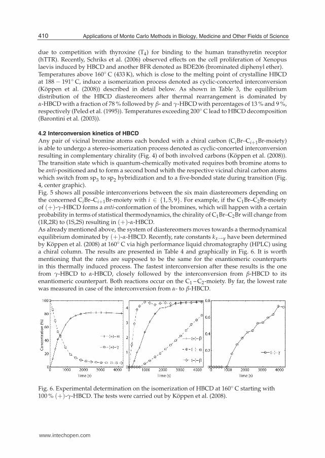
Any pair of vicinal bromine atoms each bonded with a chiral carbon (CiBr–Ci+1Br-moiety)is able to undergo a stereo-isomerization process denoted as cyclic-concerted interconversionresulting in complementary chirality (Fig. 4) of both involved carbons (Köppen et al. (2008)).The transition state which is quantum-chemically motivated requires both bromine atoms tobe anti-positioned and to form a second bond whith the respective vicinal chiral carbon atomswhich switch from sp3 to sp2 hybridization and to a five-bonded state during transition (Fig.4, center graphic).Fig. 5 shows all possible interconverions between the six main diastereomers depending onthe concerned CiBr–Ci+1Br-moiety with i ∈ {1, 5, 9}. For example, if the C1Br–C2Br-moietyof (+)-γ-HBCD forms a anti-conformation of the bromines, which will happen with a certainprobability in terms of statistical thermodynamics, the chirality of C1Br–C2Br will change from(1R,2R) to (1S,2S) resulting in (+)-α-HBCD.As already mentioned above, the system of diastereomers moves towards a thermodynamicalequilibrium dominated by (+)-α-HBCD. Recently, rate constants kx→y have been determinedby Köppen et al. (2008) at 160◦ C via high performance liquid chromatography (HPLC) usinga chiral column. The results are presented in Table 4 and graphically in Fig. 6. It is worthmentioning that the rates are supposed to be the same for the enantiomeric counterpartsin this thermally induced process. The fastest interconversion after these results is the onefrom γ-HBCD to α-HBCD, closely followed by the interconversion from β-HBCD to itsenantiomeric counterpart. Both reactions occur on the C1 – C2-moiety. By far, the lowest ratewas measured in case of the interconversion from α- to β-HBCD.

Fig. 6. Experimental determination on the isomerization of HBCD at 160◦ C starting with100 % (+)-γ-HBCD. The tests were carried out by Köppen et al. (2008).


www.intechopen.com

Interconversion CiBr–Ci+1Br-moiety Rate constant k[

mol(%)s

]

kα→β C5 – C6/C9 – C10 1.88 ± 0.01 × 10−5

kα→γ C1 – C2 1.42 ± 0.01 × 10−4

kβ→α C9 – C10 1.20 ± 0.01 × 10−4

kβ→β C1 – C2 1.10 ± 0.03 × 10−3

kβ→γ C5 – C6 1.70 ± 0.01 × 10−4

kγ→α C1 – C2 1.50 ± 0.01 × 10−3

kγ→β C5 – C6/C9 – C10 1.46 ± 0.01 × 10−4

Table 4. Rate constants ky→z with y, z ∈ {α, β, γ} for the cyclic-concerted interconversionprocess of HBCD at 160◦ C.

5. Simulation of HBCD interconversion rates

As already mentioned in section 4, the six main HBCD diastereomers underly a isomerizationprocess at temperatures between 433 and 473 K denoted as cyclic-concerted interconversion(see Fig. 5) which is quantum-chemically motivated and results in complementary chiralityof both concerned vicinal brominated carbon atoms. Nevertheless, this section presents anapproach for estimating transition rates of such processes in terms of classical mechanics.It is due to the matter of time scale and the complexity of electronic densities, that theinterconversion can hardly be investigated by quantum-chemical methods without enormouscomputational costs.Due to high rotational barriers, high-temperature simulations are inevitable in orderto avoid trapping effects. Hence, the adoption of these results to lower temperaturesrequires a reweighting strategy which has been developed within the framework of theseinvestigations. Afterwards, the interconversion rates are approximated on the basis of freeenergy calculations in combination with the Arrhenius equation and by applying the transitionstate theory (TST). Fortunately, experimental data of the interconversion kinetics is availableand will be compared to the theoretical results obtained here.

5.1 Classical model for the interconversion

A necessary condition for the transition state of interconversion processes is theanti-positioning of two vicinal bromine atoms in liquid phase, that we will call an “activestate”. It is assumed to occur more likely with lower rotational barriers between anti andgauche conformations and vice versa. The rate of the transition is considered to depend onboth, the probability of such an activated state, which can be described in terms of classicalthermodynamics and the velocity of the quantum-chemically motivated transition itself. Thelatter may simply be neglected due to the assumption of its identity in case of all HBCDdiastereomers. Therefore, a qualitative definition of interconversion rates in terms of freeenergy differences only between two subsets Ωanti and Ωgauche ∈ R

3n of the conformational

space Ω ∈ R3n turns out to be a suitable approach.

Initially, a sampling of the conformational space had to be performed with the HMC methodat an artificially high temperature T=1500 K (i. e. with the Boltzmann factor β0 =0.0802 mol/kJand in vacuum, neglecting mutual interactions with other HBCD molecules or with asolvent such as water and therefore, reducing computational costs. We decided to utilizethe Merck molecular force �eld (mmff) designed by Halgren (1996) for our simulations. Foreach diastereomer, five trajectories were constructed each consisting of 100.000 MC stepswith 60 MD steps per MC step. The MD integration step was set to 1.3 fs. Convergence was


www.intechopen.com

checked in accordance with Gelman & Rubin (1992) on the basis of the five Markov chains. Theconjugate gradient (CG) minimization method (Hestenes & Stiefel (1952)) was used for energyoptimization of the sampled geometries in order to identify all local and thus, global minima.The free energy A(β) is defined in terms of the partition function

A(β) = −1

βln

(∫

Ωexp (−βV (q)) dq

). (12)

Note, that the kinetic part K(p) of the total energy H(q, p) is missing due to the assumptionof its idendity for both conformational subsets at identical temperature. In this section, wewill only consider the potential energy fraction V(q) of the separable Hamiltonian. It isnot possible to approximate the integral in Equation 12; however, free energy differencesΔgaA(β) (a = anti, g = gauche) of two conformational subsets Ωanti and Ωgauche maybe approximated. Due to importance sampling (compare Equation 5 with 6), the number

of geometries containing anti- (Nanti) and gauche-conformation(Ngauche

), respectively,

according to the CiBr–Ci+1Br-moiety under consideration is sufficiant in order to approximate

ΔgaA(β) ≈ −1

βln

(Ngauche

Nanti

). (13)

A dihedral angle θ between two vicinal bromine atoms was defined as anti if |θ| > 120◦ , i. e. ifthe lower bromine atom remained in the grey-coloured segment as depicted in Fig. 7, whereasan angle 120 ≥ θ ≥ −120 ◦ was defined as gauche.

Fig. 7. For the interconversion anlysis, the bromine’s conformation was defined as anti if thedihedral θ was greater than 120 ◦ and less than −120 ◦ (lower bromine within the greysegment).

These free energy differences were calculated for each CiBr–Ci+1Br-moiety of all (+)-HBCDenantiomers. The lower the free energy difference, the more the state indicated by the firstindex (g = gauche) is preferred.In the followings, we will additionally need another thermodynamic quantity derivedfrom the simulated data, namely the mean potential energy 〈V〉 defined as a function oftemperature β

〈V〉 (β) =∫

ΩV (q)

exp (−βV (q))∫Ω

exp (−βV (q)) dqdq (14)

which can be approximated by the arithmetic mean of all potential energy valuesfrom the HMC sampling. Again, the energy difference Δga 〈V〉 was determined foreach CiBr–Ci+1Br-moiety of all (+)-HBCD enantiomers, after having partitioned theconformational space Ω into gauche and anti subsets and having calculated their respectivemean potential energies.


www.intechopen.com

5.2 Thermodynamical energy reweighting

The HMC sampling had been performed at temperature T = 1500 K (β0 = 0.0802 mol/kJ)due to convergence reasons. However, we are interested in the energy distribution at T =433 K (β1 = 0.2778 mol/kJ) which marks the melting point of HBCD. Usually, reweighting isunderstood in a point-wise way, reweighting the complete distribution to the temperature ofinterest and, therefore, statistically weighting up a relatively small number of points in theoverlap region of both the high- and the low-temperature distribution (see grey coloured areain Fig. 8).

Fig. 8. Overlap region between high and low potential energy distributions relevant forpoint-wise reweighting.

Here, we apply a thermodynamical approach instead of a point-wise one, making use ofthe temperature-dependency of the distribution’s mean value, i. e. its dependency on β. Inanalogy to the mean kinetic energy 〈K〉, we assume a linear dependency of the mean potentialenergy 〈V〉 on the temperature T (i. e. on β−1)

Δga 〈V〉 (β) =

[Δga 〈V〉 (β0) − Δga 〈V〉 (∞)

]β0

β+ Δga 〈V〉 (∞). (15)

ΔgaV (∞) denotes the difference of the global minimal energies of both subspaces at absolutezero T = 0 K ⇔ β = ∞. Since the system moves towards the global optimum with decreasingtemperature, a conjugate gradient minimization was applied to the complete canonicalhigh-temperature ensembles of HBCD geometries. Again, each CiBr–Ci+1Br-moiety of all(+)-HBCD enantiomers underwent this procedure after having been separated according totheir anti/gauche-isomerization. In addition and via Equation 15, mean potential energies andtheir differences for each CiBr–Ci+1Br-moiety can now be interpolated to the temperature ofinterest which is the melting point of HBCD at 433 K. See Fig. 9 for a graphical representationof the linear model.However, in order to determine interconversion rates as described in the next section, freeenergy differences for each CiBr–Ci+1Br-moiety at the desired temperature needed to beestimated as well. This was achieved by first differentiating Equation 12 and insertingEquation 14

d

dβΔgaA (β) = −

1

βΔgaA (β) +

1

βΔga 〈V〉 (β). (16)

Inserting the linear model (Equation 15) instead of the last term of Equation 16 leads to theordinary differential equation

d

dβΔgaA (β) = −

1

βΔgaA (β) +

[Δga 〈V〉 (β0)− ΔgaV(∞)

]β0

β2+

ΔgaV(∞)

β. (17)


www.intechopen.com

Fig. 9. A linear model for the thermodynamical reweighting of mean potential energies totemperatures between the one used for high-temperature simulations and absolute zero.

which can be solved analytically, such that

ΔgaA (β) =β − β0

βΔga 〈V〉 (∞)

+β0

βln

(β

β0

) [Δga 〈V〉 (β0) − Δga 〈V〉 (∞)

]+

β0

βΔgaA (β0) .

(18)

Equation 18 allows to interpolate free energy differences for temperatures such as the desiredone at T = 433 K.

5.3 Rate matrix and interconversion kinetics

Basically, the estimation of interconversion rates rested upon the combination of the Arrheniusequation (Göpel & Wiemdörfer (2000)) with the transition state theory (TST) (Weber (2007)).According to Arrhenius, the reaction rate k depends on the temperature T (respectively β) andon the activation energy EA as follows

k = A · exp (−βEA) (19)

with a prefactor A. In this work, the activation energy for the interconversion process at acertain CiBr–Ci+1Br-moiety requiring anti conformation was approximated by the free energydifference between the respective subspaces of the conformational space, due to an obviousdependency of the interconversion rate k from the free energy difference ΔagA = −ΔgaA.In other words, the higher the free energy difference between the gauche and anti subspaceis, the more likely the system is to form anti conformations and, therefore, the larger theinterconversion rate will be. Hence, we propose this correlation such that

k ∝ exp(−βΔagA

)(20)

neglecting the prefactor from Equation 19 which needs to be determined experimentally andmarks an upper bound for the maximal reaction rate. As we do not expect to gain quantitative,but qualitative interconversion rates, the prefactor does not play any role for our purposes.


www.intechopen.com

These rates were used now to fill up non-zero entries of the squared matrix K ∈ R6×6 with

one dimension per HBCD diastereomer in the order (+) -α, (+) -β, (+) -γ, (−) -α, (−) -β,(−) -γ. For example, the element of the third row ((+) -γ = educt) and the first column((+) -α = product) of K is determined by

k3,1 = k(+)γ→(+)α = exp(−βΔagA

)(21)

where ΔagA is the free energy difference for anti and gauche conformations of the accordingC1Br–C2Br-moiety, derivable from Fig. 5. Note, that the interconversion from α- or γ- toβ-HBCD is associated with two CiBr–Ci+1Br-moieties (C5Br–C6Br and C9Br–C10Br). Here,both respective free energy differences must be summed up before being inserted intoEquation 21.K is a stochastic matrix with the row sums needing to be scaled to 1. It is also denoted asembedded Markov chain playing a central role in the TST, particularly for the computation of therate matrix Q ∈ R

6×6 we are interested in

Q = R (K− id) (22)

where id denotes the six-dimensional unit matrix and R ∈ R6×6 the diagonal matrix of rate

facors (Kijima (1997); Weber (2007)). Q is well-known from the first order rate equation

dx (t)

dt= Q⊤x (t) (23)

describing changes of the concentration vector x ∈ R6 over time t using the (transposed)

rate matrix Q. In case of equilibrium concentrations x (t) = π (t) at the systems steady-state,Equation 23 becomes

dπ (t)

dt= Q⊤π (t) = 0 ⇐⇒ π⊤Q = 0. (24)

This information is necessary for the computation of the matrix R of rate factors which is thelast unknown quantity in Equation 22. For this purpose, the right-hand side of equation 22was inserted into Q of the second part of Equation 24 resulting in

π⊤R (K− id) = 0. (25)

Little manipulations of Equation 25 lead us to the eigenproblem

r⊤Π (K− id) = 0 · r⊤ (26)

where the diagonal elements of the diagonal matrix R have been transferred into an ordinaryvector r and vice versa in case of the steady-state distribution vector π which was transformedinto a diagonal matrix Π. This is a sophisticated way to solve rate factors r (and hence, R andQ), handling them as an eigenvector of the eigenvalue zero. A simulation of these theoreticalinterconversion kinetics can be performed by solving the differential Equation 23 such that

x (τ) = x (0) exp (τQ) (27)

starting at an initial distribution x (0) and iterating over a time span t = τ. All calculationshave been performed with the software Matlab.


www.intechopen.com

6. Results and discussion

6.1 HMC-sampling of HBCD diastereomers

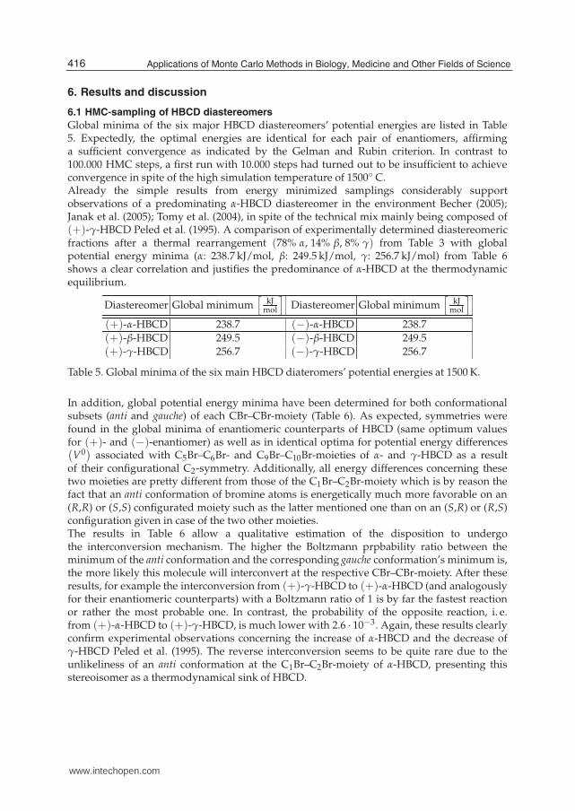
Global minima of the six major HBCD diastereomers’ potential energies are listed in Table5. Expectedly, the optimal energies are identical for each pair of enantiomers, affirminga sufficient convergence as indicated by the Gelman and Rubin criterion. In contrast to100.000 HMC steps, a first run with 10.000 steps had turned out to be insufficient to achieveconvergence in spite of the high simulation temperature of 1500◦ C.Already the simple results from energy minimized samplings considerably supportobservations of a predominating α-HBCD diastereomer in the environment Becher (2005);Janak et al. (2005); Tomy et al. (2004), in spite of the technical mix mainly being composed of(+)-γ-HBCD Peled et al. (1995). A comparison of experimentally determined diastereomericfractions after a thermal rearrangement (78% α, 14% β, 8% γ) from Table 3 with globalpotential energy minima (α: 238.7 kJ/mol, β: 249.5 kJ/mol, γ: 256.7 kJ/mol) from Table 6shows a clear correlation and justifies the predominance of α-HBCD at the thermodynamicequilibrium.

Diastereomer Global minimum[

kJmol

]Diastereomer Global minimum

[kJ

mol

]

(+)-α-HBCD 238.7 (−)-α-HBCD 238.7

(+)-β-HBCD 249.5 (−)-β-HBCD 249.5

(+)-γ-HBCD 256.7 (−)-γ-HBCD 256.7

Table 5. Global minima of the six main HBCD diateromers’ potential energies at 1500 K.

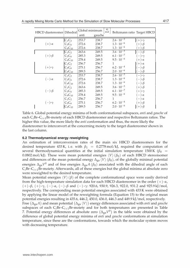
In addition, global potential energy minima have been determined for both conformationalsubsets (anti and gauche) of each CBr–CBr-moiety (Table 6). As expected, symmetries werefound in the global minima of enantiomeric counterparts of HBCD (same optimum valuesfor (+)- and (−)-enantiomer) as well as in identical optima for potential energy differences(V0

)associated with C5Br–C6Br- and C9Br–C10Br-moieties of α- and γ-HBCD as a result

of their configurational C2-symmetry. Additionally, all energy differences concerning thesetwo moieties are pretty different from those of the C1Br–C2Br-moiety which is by reason thefact that an anti conformation of bromine atoms is energetically much more favorable on an(R,R) or (S,S) configurated moiety such as the latter mentioned one than on an (S,R) or (R,S)configuration given in case of the two other moieties.The results in Table 6 allow a qualitative estimation of the disposition to undergothe interconversion mechanism. The higher the Boltzmann prpbability ratio between theminimum of the anti conformation and the corresponding gauche conformation’s minimum is,the more likely this molecule will interconvert at the respective CBr–CBr-moiety. After theseresults, for example the interconversion from (+)-γ-HBCD to (+)-α-HBCD (and analogouslyfor their enantiomeric counterparts) with a Boltzmann ratio of 1 is by far the fastest reactionor rather the most probable one. In contrast, the probability of the opposite reaction, i. e.from (+)-α-HBCD to (+)-γ-HBCD, is much lower with 2.6 · 10−3. Again, these results clearlyconfirm experimental observations concerning the increase of α-HBCD and the decrease ofγ-HBCD Peled et al. (1995). The reverse interconversion seems to be quite rare due to theunlikeliness of an anti conformation at the C1Br–C2Br-moiety of α-HBCD, presenting thisstereoisomer as a thermodynamical sink of HBCD.


www.intechopen.com

HBCD diastereomer DihedralGlobal minimum

[kJ

mol

]Boltzmann ratio Target HBCD

anti gauche

(+)-αC1C2 253.7 238.7 2.6 · 10−3 (+)-γC5C6 272.6 238.7 1.3 · 10−6 (+)-βC9C10 272.6 238.7 1.3 · 10−6 (+)-β

(+)-βC1C2 263.6 249.5 3.6 · 10−3 (−)-βC5C6 285.3 249.5 6.1 · 10−7 (−)-γC9C10 278.4 249.5 9.5 · 10−6 (+)-α

(+)-γC1C2 256.7 256.7 1 (+)-αC5C6 275.1 256.7 6.2 · 10−4 (−)-βC9C10 289.5 256.7 2.0 · 10−6 (−)-β

(−)-αC1C2 253.7 238.7 2.6 · 10−3 (−)-γC5C6 272.6 238.7 1.3 · 10−6 (−)-βC9C10 272.6 238.7 1.3 · 10−6 (−)-β

(−)-βC1C2 263.6 249.5 3.6 · 10−3 (+)-βC5C6 285.3 249.5 6.1 · 10−7 (+)-γC9C10 278.4 249.5 9.5 · 10−6 (−)-α

(−)-γC1C2 256.7 256.7 1 (−)-αC5C6 275.1 256.7 6.2 · 10−4 (+)-βC9C10 289.5 256.7 2.0 · 10−6 (+)-β

Table 6. Global potential energy minima of both conformational subspaces, anti and gauche ofeach CiBr–Ci+1Br-moiety of each HBCD diastereomer and respective Boltzmann ratios. Thehigher this value, the more likely the anti conformation and thus, the more likely thediastereomer to interconvert at the concerning moiety to the target diastereomer shown inthe last column.

6.2 Thermodynamical energy reweighting

An estimation of interconversion rates of the main six HBCD diastereomers for thedesired temperature 433 K, i. e. with β1 = 0.2778 mol/kJ, required the computation ofseveral thermodynamical quantities at the initial simulation temperature 1500 K (β0 =0.0802 mol/kJ). These were mean potential energies 〈V〉 (β0) of each HBCD stereoisomerand differences of the mean potential energy Δga 〈V〉 (β0), of the globally minimal potential

energies ΔgaV0 and of free energies ΔgaA (β0) associated with the dihedral angle of each

CiBr–Ci+1Br-moiety. Afterwards, all of these energies but the global minima at absolute zerowere reweighted to the desired temperature.Mean potential energies 〈V〉 (β) of the complete conformational space were easily derivedfrom the high-temperature simulation data for each HBCD diastereomer in the order (+) -α,(+) -β, (+) -γ, (−) -α, (−) -β and (−) -γ: 920.6, 930.9, 926.3, 922.0, 931.2 and 925.9 kJ/mol,respectively. The correponding mean potential energies associated with 433 K were obtainedby applying the linear model of the reweighting formula (Equation 15) to the original meanpotential energies resulting in 435.6, 446.2, 450.0, 436.0, 446.3 and 449.9 kJ/mol, respectively.Free

(ΔgaA

)and mean potential

(Δga 〈V〉

)energy differences associated with anti and gauche

subspaces of each CiBr–Ci+1Br-moiety and for both temperatures are presented in Table7. Potential energy differences at absolute zero

(ΔgaV

0)

in the table were obtained by thedifference of global potential energy minima of anti and gauche conformations at simulationtemperature, since these are the conformations, towards which the molecular system moveswith decreasing temperature.


www.intechopen.com

Diastereomer DihedralEnergies at T = 1500 K

[kJ

mol

]At T = 433 K

[kJ

mol

]Target

Δga 〈V〉 ΔgaV0 ΔgaA Δga 〈V〉 ΔgaA

(+)-αC1C2 −7.8 −14.9 −16.7 −10.4 −12.9 (+)-γC5C6 −26.0 −33.9 −40.4 −30.2 −32.9 (+)-βC9C10 −25.6 −33.9 −39.7 −29.7 −32.6 (+)-β

(+)-βC1C2 −0.3 −14.0 −14.3 −4.3 −9.2 (−)-βC5C6 −19.9 −35.8 −35.5 −24.4 −30.0 (−)-γC9C10 −17.5 −26.7 −34.0 −22.2 −25.5 (+)-α

(+)-γC1C2 4.8 0.0 −9.7 0.6 −1.1 (+)-αC5C6 −28.3 −18.5 −41.3 −32.0 −28.6 (−)-βC9C10 −27.1 −18.5 −41.0 −31.1 −28.1 (−)-β

(−)-αC1C2 −6.9 −14.9 −16.7 −9.8 −12.6 (−)-γC5C6 −24.4 −33.9 −38.0 −28.3 −31.7 (−)-βC9C10 −21.9 −33.9 −38.1 −26.6 −30.8 (−)-β

(−)-βC1C2 −1.7 −14.0 −13.5 −5.1 −9.5 (+)-βC5C6 −19.1 −35.8 −35.3 −23.7 −29.6 (+)-γC9C10 −15.0 −26.7 −35.9 −21.1 −25.2 (−)-α

(−)-γC1C2 3.1 0.0 −11.0 −1.0 −2.1 (−)-αC5C6 −31.3 −18.5 −42.5 −34.5 −30.0 (+)-βC9C10 −30.9 −18.5 −42.2 −34.1 −29.8 (+)-β

Table 7. Mean potential(Δga 〈V〉

)and free

(ΔgaA

)energies of both conformational

subspaces (anti and gauche) of each CiBr–Ci+1Br-moiety of each HBCD diastereomer at thesimulation temperature T = 1500 K and reweighted to the desired temperature at T = 433 K,respectively as well as potential energy differences at T= 0 K, i. e. potential energydifferences of the concerning global minima

(ΔgaV

0)

gained by sampling at T = 1500 K andminimizing.

The estimated equilibrium distribution for 433 K presented in section 6.3 is similar to theexperimentally determined distribution after thermal rearrangement Peled et al. (1995). Bothmethods provide a by far highest fraction of (+)-α-HBCD and decreasing fractions in theorder (+)-β-HBCD and (+)-γ-HBCD. If the mean potential energies had been chosen to beinterpolated to 630 K instead, the estimated equilibrium distribution would have resulted inequal values with a relative error of only 10 %, which is not presented among these results.

6.3 HBCD interconversion rates and kinetics

By inserting the negated free energy differences from the last but one column of Table 7 intothe modified Arrhenius Equation 21, the embedded Markov chain was calculated first:

K =

⎛⎜⎜⎜⎜⎝

0 0.0080 0.9920 0 0 00.0107 0 0 0 0.9863 0.00310.9990 0 0 0 0.0010 0

0 0 0 0 0.0112 0.98880 0.9838 0.0037 0.0126 0 00 0.0009 0 0.9991 0 0

⎞⎟⎟⎟⎟

.

This matrix contains a 0 whenever a interconversion is not possible. Only the 14interconversions as depicted in Fig. 5 lead to values greater than 0 in matrix K. Row sumswere scaled to 1.The steady-state distribution π of HBCD at 433 K was determined by inserting thecorresponding mean potential energy values, interpolated to this temperature as shown


www.intechopen.com

above, into the potential energy part of the Boltzmann expression, neglecting the partionfunction but scaling the sum to 1:

π⊤ = (0.4912 0.0258 0.0090 0.4396 0.0251 0.0092)

This vector gives evidence about a theoretical distribution of HBCD diastereomers. Summingup the first and forth value of π, i. e. the molar fractions of (+)- and (−)-α-HBCD yields 93.1 %for α-HBCD and analogously, in case of β- and γ-HBCD 5.1 % and 1.8 %, respectively.After having solved the eigenproblem of Equation 26, the theoretical rate matrix Q wasdetermined

Q = μ ·

⎛⎜⎜⎜⎜⎝

−0.0184 0.0001 0.0183 0 0 00.0023 −0.2200 0 0 0.2170 0.00070.9990 0 −1.0000 0 0.0010 0

0 0 0 −0.0167 0.0002 0.01660 0.2231 0.0008 0.0028 −0.2267 00 0.0007 0 0.7879 0 −0.7886

⎞⎟⎟⎟⎟

up to an unknown scaling factor μ which is due to the unknown velocity of the interconversionprocess. Consequently, simulation of the interconversion kinetics was performed now byapplying Equation 27 to an initial distribution x(0)

x⊤(0) =(0 0 1 0 0 0

)

with a discretized time step Δτ = 1 over a time span of τ = 4000 “seconds” and anarbitrary scaling factor μ = 0.007 resulting in interconversion kinetics as shown in Fig. 10. Theinitial distribution with 100 % (+)-γ-HBCD was chosen in accordance with the experimentalsetup which had led to the experimental kinetics depicted in Fig. 6. After these completelytheoretical results of HBCD interconversion kinetics starting at 100 % (+)-γ-HBCD (Fig.10) as also done in the laboratory, the concentration of this stereoisomer rapidly decreaseswith the highest rate reaching its equilibrium value already after 1000 “seconds”, whilethe concentration of (+)-α-HBCD increases with nearly the same velocity far above itsequilibrium value. A longer simulation that is not presented here shows an subsequentdecrease towards its equilibrium. The β diastereomers are the next ones to increase towardstheir steady-state concentration with (−)-β-HBCD starting slightly faster due to its creationfrom (+)-γ-HBCD. But with increasing (+)-α-HBCD, (+)-β-HBCD, which evolves from(+)-α-HBCD, accumulates faster and overtakes (−)-β-HBCD. The by far slowest growth isin the case of (−)-γ-HBCD.From a qualitative point of view, all these observations on the kinetics correspond exactlywith experimental results (Köppen et al. (2008)) as presented in Fig. 6 and Table 4. The highestand second highest rate was confirmed to be kγ→α and kβ→β, respectively, whereas kα→β

(Q (1, 2) and Q (4, 5)) yielded the lowest value with both approaches. Many assumptionswere necessary in order to estimate interconversion rates for the six main HBCD isomers,started off with the vacuum approximation, neglecting any intermolecular interactions in theliquid phase and by the way, reducing the computational effort. Due to sterical reasons andthe fact of poor solubility in a polar medium such as water (Janak et al. (2005)), we claim anegligible affect of intermolecular interactions on the interconversion process.Describing the quantum-chemically motivated inversion process in terms of classicalmechanics was a second bold approximation. However, if we consider its rate as acombination of the probability of being activated (anti conformation) and the transition itselfand under the assumption of an identical velocity of the latter part for all diastereomers, we


www.intechopen.com

Fig. 10. theoretical determinantion of the HBCD isomerization at 160 C starting at 100 %(+)-γ-HBCD and with a scale factor μ = 0.007. Free and potential energy values had beenreweighted after a high-temperature HMC simulation at 1500 K.

are able to reduce the interconversion to a classical manner with its rate characterized bydifferences of energies/probabilities between anti and gauche subspaces, i. e. the differencein free energies expressing the likeliness of a molecular system to adopt the one or theother conformation. What we lose by this simplification is the knowledge about the absolutevelocities of the interconversion and thus, the opportunity to describe rates quantitatively. Butwhat we gain is the ability to calculate this quantum-chemical process (in reasonable time).Also the application of the Arrhenius equation to these free energy differences might seem alittle far-fetched, but again, there is an obvious correlation between the free energy differenceand the ordinary activation energy. Both describe the delay of energies from an arbitrarilyfixed value, differing in accordance with the direction of the reaction. In other words, ifthe activation energy is low for the forward direction, then the free energy difference islow as well. From the reverse perspective, the free energy difference increases, too, if theactivation energy increases. Similar to the free energy difference, the activation energy maybe considered in this context as the energy necessary to lead the molecules to the active anticonformation. Still, we are able to gain qualitative or even semi-quantitative results.As we were interested in the kinetics of the HBCD system at 433 K, a reweighting of energyvalues became unavoidable. Instead of a point-wise scheme that weights up a probably smallnumber of values from the overlap region of high- and low-temperature distributions, wedecided to apply a thermodynamical approach assuming a linear temperature-dependency ofthe mean potential energy (Equation 15). If the potential energy V was a quadratic functionin the onformational space Ω, this assumption would be true. However, the potential energyfunction is not an exact quadratic one but is locally approximable by parabolic functions dueto its Gaussian-like distributions in a accordingly decomposed conformational space.In spite of all these approximations, the results well reflect the HBCD interconversion processas determined by experimental methods, and in particular, no experimental data was used forthe estimation at all.

7. References

Akhmatskaya, E. & Reich, S. (2004). The targeted shadowing hybrid Monte-Carlo (tshmc)method, Technical report, Institut für Mathematik, Uni Potsdam.

Allen, M. P. & Tildesley, D. J. (1987). Computer Simulations of Liquids, Clarendon, Oxford.Andersen, H. C. (1980). Molecular dynamics simulations at constant pressure and/or

temperature, J.Chem.Phys. 72: 2384–2393.


www.intechopen.com

Barda, H. J., Sanders, D. C. & Benya, T. J. (1985). Bromine compounds, in S. Hawkins& G. Schultz (eds), Ullmann’s Encyclopedia of Industrial Chemistry, Wiley-VCH,Weinheim, Germany, pp. 405–429.

Barontini, F., Cozzani, V. & Petarca, L. (2003). Thermal stability and decomposition productsof hexabromocyclododecane, Ind. Eng. Chem. Res. 40: 3270–3280.

Becher, G. (2005). The stereochemistry of 1,2,5,6,9,10-hexabromocyclododecane and itsgraphic representation, Chemosphere 58: 989–991.

Binder, K. & Landau, D. (2000). A Guide to Monte Carlo Simulations in Statistical Physics,Cambirdge University Press, Cambirdge.

Clamp, M. E., Baker, P. G., Stirling, C. J. & Brass, A. (1994). Hybrid Monte Carlo: An efficientalgorithm for condensed matter simulation, J.Comput.Chem. 15(8): 838–846.

Covaci, A., Gerecke, A. S. C., Voorspoels, R. J. L. S., Kohler, M., Heeb, N. V., Leslie, H., Allchin,C. R. & DeBoer, J. (2006). Hexabromocyclododecanes (HBCDs) in the environmentand humans: a review, Environ. Sci. Techno. 40: 3680–3688.

de Wit, C. A., Alaee, M. & Muir, D. C. G. (2006). Levels and trends of brominated flameretardants in the arctic, Chemosphere 64: 209–233.

de Witt, C. A. (2002). An overview of brominated flame retardants in the environment,Chemosphere 46: 583–624.

Deuflhard, P. (1983). Order and stepsize control in extrapolation methods, Numer. Math.pp. 399–422.

Deuflhard, P. (1985). Recent progress in extrapolation methods for ordinary differentialequations, SIAM Review 27: 505–535.

Deuflhard, P., Dellnitz, M., Junge, O. & Schütte, C. (1999). Computation of essential moleculardynamics by subdivision techniques, in P. D. et al (ed.), Computational MolecularDynamics: Challenges, Methods, Ideas, Springer, Berlin, pp. 98–115.

Duane, S., Kennedy, A. D., Pendleton, B. J. & Roweth, D. (1987). Hybrid Monte Carlo, Phys.Lett. B 195(2): 216–222.

Fischer, A. (1997). Die Hybride Monte–Carlo Methode in der Molekülphysik. Diplomathesis, Department of Mathematics and Computer Science, Free University Berlin,(in German).

Fischer, A., Cordes, F. & Schütte, C. (1998). Hybrid Monte Carlo with adaptive temperaturein a mixed–canonical ensemble: Efficient conformational analysis of RNA, J. Comput.Chem. 19: 1689–1697.

Forrest, B. M. & Suter, U. W. (1994). Hybrid Monte Carlo simulations of dense polymersystems, J.Chem.Phys. 101.

Frenkel, D. & Smit, B. (1996). Understanding molecular simulation. From algorithms to applications,Academic Press, San Diego.

Frenkel, D. & Smit, B. (2002). Understanding Molecular Simulation – From Algorithms toApplications, Vol. 1 of Computational Science Series, 2nd edn, Academic Press, ADivision of Harcourt, Inc., www.academicpress.com/computationalscience.

Gelman, A. & Rubin, D. (1992). Inference from Iterative Simulation using Multiple Sequences,Statist. Sci. 7: 457–511.

Göpel, W. & Wiemdörfer, H. D. (2000). Statistische Thermodynamik, Spektrum AkademischerVerlag.

Griebel, M., Zumbusch, G. & Knapek, S. (2007). Numerical Simulation in Molecular Dynamics,Vol. 5 of Texts in Computational Science and Engineering, Springer, Berlin.


www.intechopen.com

Gromov, D. G. & de Pablo, J. J. (1995). Structure of binary polymer blends - multiple timestep hybrid Monte Carlo simulations and self-consistend intergal-equation theory,J.Chem.Phys. 103(18): 8247–8256.

Gupta, S., Irbäck, A., Karsch, F. & Petersson, B. (1990). The acceptance probability in the hybridMonte Carlo method, Phys. Lett. B 242: 437–443.

Hairer, E., Lubich, C. & Wanner, G. (2004). Geometric Numerical Integration –Structure-Preserving Algorithms for Ordinary Differential Equations, Vol. 31 of SpringerSeries in Computational Mathematics, corr. 2nd edn, Springer.

Hairer, E., Nørsett, S. P. & Wanner, G. (1993). Solving Ordinary Differential Equations I, NonstiffProblems, 2nd edn, Springer-Verlag, Berlin, Heidelberg.

Hale, R. C., La Guardia, M. J., Harvey, E., Gaylor, M. O., Matt, T. & Mainor, T. M. (2006).Brominated flame retardant concentrations and trends in abiotic media, Chemosphere64: 181–186.

Halgren, T. A. (1996). Merck Molecular Force Field: I-V, J. Comp. Chem. 17(5-6): 490–641.Hamers, T., Kamstra, J. H., Sonneveld, E., Murk, A. J., Kester, M. H. A., Andersson, P. L., Legler,

J. & Brouwer, A. (2006). In Vitro Profiling of the Endocrine-Disrupting Potency ofBrominated Flame Retardants, Toxicol. Sci. 92: 157–173.

Hammersley, J. & Handscomb, D. (1964). Monte Carlo Methods, J. Wiley, New York.Hansmann, U. H. E., Okamoto, Y. & Eisenmenger, F. (1996). Molecular dynamics, Langevin

and hybrid Monte Carlo simulations in a multicanonical ensemble, Chem.Phys.Lett.259: 321–330.

Heeb, N. V., Schweizer, W. B., Kohler, M. & Gerecke, A. C. (2004).1,2,5,6,9,10-hexabromocyclododecane - a class of compounds with a complexstereochemistry, Book of abstracts, Toronto, Canada, pp. 337–340. The ThirdInternational Workshop on Brominated Flame Retardants.

Heeb, N. V., Schweizer, W. B., Mattrel, P., Haag, R., Kohler, M., Schmid, P., Zennegg,M. & Wolfensberger, M. (2008). Regio- and stereoselective isomerizationof hexabromocyclododecanes (HBCDs): Kinetics and mechanism of β-HBCDracemization, Chemosphere 71: 1547–1556.

Hestenes, M. R. & Stiefel, E. (1952). Methods of Conjugate Gradients for Solving LinearSystems, J. Res. Nat. Inst. Stand. Technol. 49: 409–436.

Hockney, R. W. (1970). The potential calculations and some applications, Methods Comput.Phys. 9: 136–211.

Hunziker, R. W., Gonsior, S., MacGregor, J. A., Desjardins, D., Ariano, J. & Friederich, U. (2004).Fate and effect of hexabromocyclododecane in the environment, OrganohalogenCompd 66: 2300–2305.

Irbäck, A. (1994). Hybrid Monte Carlo simulation of polymer chains, J.Chem.Phys.101(2): 1661–1667.

Izaguirre, J. A. & Hampton, S. S. (2004). Shadow hybrid Monte Carlo: An efficient propagatorin phase space of macromolecules, J. Comput. Phys. 200: 581–604.

Janak, K., Covaci, A., Voorspoels, S. & Becher, G. (2005). Hexabromocyclododecane in marinespecies from the western Scheldt estuary: diastereoisomer- and enantiomer-specificaccumulation, Environ. Sci. Technol. 39: 1987–1994.

Johnson-Restrepo, B., Adams, D. H. & Kannan, K. (2008). Tetrabromobisphenol A (TBBPA)and hexabromocyclododecanes (HBCDs) in tissues of humans, dolphins, and sharksfrom the United States, Chemosphere 70(11): 935–1944.


www.intechopen.com

Kennedy, A. D. & Pendleton, B. (1991). Acceptances and autocorrelation in hybrid MonteCarlo, Nuclear Physics B Proceedings Supplements 20: 118–121.

Kijima, M. (1997). Markov Processes for Stochastic Modeling, Stochastic Modeling Series,Chapman and Hall.

Köppen, R., Becker, R., Jung, C. & Nehls, I. (2008). On the thermally induced isomerisation ofhexabromocyclododecane stereoisomers, Chemosphere 71: 656–662.

Law, K., Palace, V. P., Halldorson, T., Danell, R., Wautier, K., Evans, B., Alaee, M., Marvin,C. & Tomy, G. T. (2006a). Dietary accumulation of hexabromocyclododecanediastereoisomers in juvenile rainbow trout (Oncorhynchus mykiss) I:Bioaccumulation parameters and evidence of bioisomerization, Environ. Toxicol.Chem. 25: 1757–1761.

Leach, A. (2001). Molecular Modelling - Principles and Applications, Pearson Educations Ltd.,Essex.

Leimkuhler, B. & Reich, S. (2004). Simulating Hamiltonian Dynamics, Cambridge.Lew, A., Marsden, J. E., Ortiz, M. & West, M. (2004). An overview of variational integrators,

in L. P. Franca, T. E. Tezduyar & A. Masud (eds), Finite Element Methods: 1970’s andBeyond, CIMNE, ISBN 84-95999-49-8, pp. 98–115.

Manousiouthakis, V. I. & Deem, M. W. (1999). Strict detailed balance is unnecessary in MonteCarlo simulation, J. Chem. Phys. 110: 2753–2756.

Meerts, I. A. T. M., van Zanden, J. J., Luijks, E. A. C., van Leeuwen-Bol, I., Marsh, G., Jakobsson,E., Bergman, A. & Brouwer, A. (2000). Potent Competitive Interactions of SomeBrominated Flame Retardants and Related Compounds with Human Transthyretinin Vitro, Toxicol. Sci. 56: 95–104.

Mehlig, B., Heermann, D. W. & Forrest, B. M. (1992). Hybrid Monte Carlo method forcondensed-matter systems, Phys.Rev. B 45(2): 679–685.

Metropolis, N., Rosenbluth, A. W., Rosenbluth, M. N., Teller, A. N. & Teller, E. (1953). Equationof state calculations by fast computing machines, J.Chem.Phys. 21: 1087–1092.

Peled, M., Scharia, R. & Sondack, D. (1995). Thermal rearrangement ofhexabromocyclododecane (HBCD), in J. R. Desmurs, B. Gérard & M. J. Goldstein(eds), Advances in Organobromine Chemistry II, Elsevier, Amsterdam, The Netherlands,pp. 92–99.

Peskun, P. (1973). Optimum Monte Carlo sampling using Marcov chains, Biometrika60: 607–612.

Robert, C. P. & Casella, G. (1999). Monte Carlo Statistical Methods, Springer New York, Berlin,Heidelberg.

Schäfer, K. (1960). Statistische Theorie derMaterie, Vol. 1, Vandenhoeck & Ruprecht in Göttingen.In German.

Schlick, T. (2002). Molecular Modelling and Simulation, Springer, New York.Schriks, M., Zvinavashe, E., Furlow, J. D. & Murk, A. J. (2006). Disruption

of thyroid hormone-mediated Xenopus laevis tadpole tail tip regression byhexabromocyclododecane (HBCD) and 2,2′,3,3′,4,4′,5,5′,6-nona brominated diphenylether (BDE206), Chemosphere 65: 1904–1908.

Skeel, R. D. & Hardy, D. J. (2002). Practical construction of modified Hamiltonians, SIAMJournal on Scienti�c Computing 23(4): 1172–1188.

Tomy, G. T., Budakowski, W., Halldorson, T., Whittle, D. M., Keir, M. J., Marvin, C., Macinnis,G. & Alaee, M. (2004). Biomagnification of α- and γ-hexabromocyclododecaneisomers in a Lake Ontario food web, Environ. Sci. Technol. 38: 2298–2303.


www.intechopen.com

Verlet, L. (1967). Computer "experiments" on classical fluids i. thermodynamical properties oflennard jones molecules, Phys. Rev. Vol. 159(No. 1): 98–103.

Vos, J. G., Becher, G., van den Berg, M., de Boer, J. & Leonards, P. E. G. (2003). Brominatedflame retardants and endocrine disruption, Pure Appl. Chem. 75: 2039–2046.

Weber, M. (2007). Conformation-Based Transition State Theory, Technical Report 07–14,Konrad-Zuse-Zentrum für Informationstechnik Berlin.

Wendlandt, J. M. & Marsden, J. E. (1997). Mechanical integrators derived from a discretevariational principle, Physica D 106: 223–246.

Zhang, H. (1999). A new hybrid Monte Carlo algorithm for protein potential function test andstructure refinement, Proteins 34: 464–471.


www.intechopen.com

Applications of Monte Carlo Methods in Biology, Medicine andOther Fields of ScienceEdited by Prof. Charles J. Mode

ISBN 978-953-307-427-6Hard cover, 424 pagesPublisher InTechPublished online 28, February, 2011Published in print edition February, 2011

InTech EuropeUniversity Campus STeP Ri Slavka Krautzeka 83/A 51000 Rijeka, Croatia Phone: +385 (51) 770 447 Fax: +385 (51) 686 166www.intechopen.com

InTech ChinaUnit 405, Office Block, Hotel Equatorial Shanghai No.65, Yan An Road (West), Shanghai, 200040, China

Phone: +86-21-62489820 Fax: +86-21-62489821

This volume is an eclectic mix of applications of Monte Carlo methods in many fields of research should not besurprising, because of the ubiquitous use of these methods in many fields of human endeavor. In an attemptto focus attention on a manageable set of applications, the main thrust of this book is to emphasizeapplications of Monte Carlo simulation methods in biology and medicine.

How to referenceIn order to correctly reference this scholarly work, feel free to copy and paste the following:

V. Durmaz, K. Fackeldey and M. Weber (2011). A rapidly Mixing Monte Carlo Method for the Simulation ofSlow Molecular Processes, Applications of Monte Carlo Methods in Biology, Medicine and Other Fields ofScience, Prof. Charles J. Mode (Ed.), ISBN: 978-953-307-427-6, InTech, Available from:http://www.intechopen.com/books/applications-of-monte-carlo-methods-in-biology-medicine-and-other-fields-of-science/a-rapidly-mixing-monte-carlo-method-for-the-simulation-of-slow-molecular-processes

A Rapidly Mixing Monte Carlo Method for the Simulation of Slow Molecular Processes

Documents

Transcript of A Rapidly Mixing Monte Carlo Method for the Simulation of Slow Molecular Processes