Biol. Cybern. 49, 127 136 (1983) Biological Cybernetics �9 Springer-Verlag 1983

A Proposed Neural Network for the Integrator of the Oculomotor System

Stephen C. Cannon s, David A. Robinson 1, and Shihab Shamma 2

1 Departments of Biomedical Engineering and Ophthalmology, The Johns Hopkins Univ., Baltimore, MD, USA 2 The National Institutes of Health, Bethesda, MD, USA

Abstract. Single-unit recordings, stimulation studies, and eye movement measurements all indicate that the firing patterns of many oculomotor neurons in the brain stem encode eye-velocity commands in premotor circuits while the firing patterns of extraocular mo- toneurons contain both eye-velocity and eye-position components. It is necessary to propose that the eye- position component is generated from the eye-velocity signal by a leaky hold element or temporal integrator. Prior models of this integrator suffer from two impor- tant problems. Since cells appear to have a steady, background signal when eye position and velocity are zero, how does the integrator avoid integrating this background rate? Most models employ some form of lumped, positive feedback the gain of which must be kept within totally unreasonable limits for proper operation. We propose a lateral inhibitory network of homogeneous neurons as a model for the neural integrator that solves both problems. Parameter sensi- tivity studies and lesion simulations are presented to demonstrate robustness of the model with respect to both the choice of parameter values and the con- sequences of pathological changes in a portion of the neural integrator pool.

1 Introduction

For the past fifteen years, oculomotor neuro- physiologists have postulated the existence of a pool of neurons that temporally integrates premotor neural commands 1 (Robinson, 1968, 1971). Cohen and Komatsuzaki (1972) were the first to provide physio- logical evidence. They found that stimulation of the paramedian zone of the pontine reticular formation

1 In this text the terms "commands" and "signals" are used interchangeably to designate neuronal discharge firing patterns which create the subsequent eye movements

(PPRF) in monkeys caused conjugate, ipsilateral, hor- izontal eye movements. During constant stimulation the eyes deviated at a constant velocity, and at the end of the stimulus the eyes remained in the new position for several hundred milliseconds, the duration of nat- ural periods of fixation. They concluded that activity induced by electrical stimulation appeared to be in- tegrated with respect to time.

The next study to support the existence of the integrator was performed by Skavenski and Robinson (1973). These authors recorded eye movements and single-unit activity of motoneurons in the abducens nucleus of the alert monkey during sinusoidal rotation in the dark. From a frequency analysis of eye and head position, they demonstrated that the total phase lag could not be accounted for by a combination of semicircular canal dynamics and the muscle and or- bital tissue lags alone. The single-unit study demon- strated a phase lag of almost 90 ~ between the firing patterns of abducens motoneurons and primary vestib- ular neurons. This is the lag that would be produced by a neural integrator.

Subsequently it has been shown that the optoki- netic system also provides an eye-velocity command that shares the integrator with the vestibular command (Waespe and Henn, 1977). Burst cells in the PPRF carry a signal proportional to eye velocity during a saccade (van Gisbergen et al., 1981) and it has been proposed that this too is integrated to provide the step change in motoneuron discharge rate that follows a saccade (Robinson, 1975). There are good physiologi- cal and theoretical reasons to suppose that all con- jugate, eye-movement systems share a common neural integrator (ibid). The concept of a neural integrator in the premotor brain-stem pathways is widely accepted, but its anatomical location and method of operation remain to be elucidated.

Two previous attempts have been made to model the neural integrator (Rosen, 1972; Kamath and

128

Keller, 1976). Rosen's model was comprised of in- dividual "neurons" that were in one of two states: either silent or firing maximally. Unfortunately, neu- rons in premotor, oculomotor areas are never seen to behave in this way. Kamath and Keller's model con- sisted of a lateral excitatory network of densely- packed, homogeneous neurons. The dynamics for an individual neuron were modelled by a first-order pro- cess with a time constant, z, of 5 ms. This value is an upper limit for z based on measurements of membrane potential transients induced by current injection (Rall, 1960). The lateral excitatory connections were reduced to a lumped parameter model of the above first-order pole and a positive feedback loop with a gain of K. The transfer function, H(s), for such a configuration is:

1 1 z H(s) = s + 1/~ - K s + 1/T. ' T~ - 1 - K z "

Becker and Klein (1973) showed, from measurements of the drift of the eye in eccentric positions in the dark, that the time constant, Tn, of the leaky, neural in- tegrator in humans is on the order of 20s. Thus in Kamath and Keller's model Kz equals 0.99975. If K were only 0.025% too large, the network would be unstable, and conversely if K were 0.4 % too small, Tn would be 1.2s, unacceptably small. Thus, as these authors pointed out, the model was unreasonably sensitive to the value of the gain of the feedback, K, - in other words the model was not robust. (Their solution to this problem - using two positive feedback loops instead of one - unfortunately does not solve the problem.) Nevertheless, their basic idea is sound and we will show that a system of reverberating collaterals can be made to work so long as one does not lump the distributed feedback into a single feedback path that requires unacceptably high tolerances.

There is an additional shortcoming of these pre- vious models. All cells that carry an eye-velocity signal, many of which presumedly serve as input to the neural integrator, have appreciable tonic or background fir- ing rates and it is the modulation about this DC component that encodes eye movement commands. The modulated component is integrated with a gain of about 2 and a time constant of 20 s. [A typical neuron carries the eye-velocity signal at 1.0 (spikes/s)/(deg/s) and the eye-position signal at 2.0 (spikes/s)/deg.] If the neural integrator functioned as a simple first-order pole with the above properties, then the DC gain would be 40. However, cells that carry an eye-position signal, many of which may be part of the neural integrator, have background firing rates approximate- ly equal to that of cells which serve as inputs to the integrator; in other words, the DC gain is about 1.0. Thus the model must be more sophisticated than a

simple first-order pole in that the gains of the back- ground and integrated components of the input must be independently controllable.

A lateral inhibitory network of linear neurons is presented below as a plausible model for the neural integrator. The properties of such networks have been studied extensively; for example see Ratline and Hartliff's monograph (1974), but usually in the context of signal or feature extraction. To our knowledge such a network has not been used before in the more humble task of integrating a single variable. We dem- onstrate that such a network indeed functions as a leaky integrator, and furthermore, the model has the virtue of both having independent gains for the DC and modulated components of the input and being robust.

2 The Model

The neural integrator is formed from a pool of homo- geneous neurons each of which inhibits the discharge rate of neighboring neurons in the pool. Most brain- stem, oculomotor neurons have firing rates that are linearly related to eye position and/or eye velocity. Thus we propose that a neuron in the neural integrator pool operates in a linear range about its background firing rate. Therefore, the integrating nature, stability, and robustness of our model do not depend on threshold or saturating nonlinearities. The firing rate of each neuron is assumed to be proportional to its transmembrane potential at the axon hillock. This so- called generator potential is in turn determined by a first-order rate process with a linear combination of dendritic influences from presynaptic cells serving as the effective input. With these assumptions the firing rate of an individual neuron is modelled as

~2(t) + x(t) = i(t),

where x(t) is the firing rate, ~ is the time constant of the first-order dynamics, and i(t) is the net, effective, presynaptic input.

The response of the ith n e u r o n in a homogeneous pool of N such neurons is described by

M N

: :2 i ( t )+xi( t )= ~ Vijuj(t ) - ~ Wljxj(t), (1) j=l j=l

where uj(t) is the firing rate of the jth input to the network, vij represents the weighting or strength of the influence of the jth input on neuron i (vii > 0 implies excitatory input, v~j < 0 implies inhibitory input), and w~j > 0 represents the weighting of the lateral inhibition exerted on the ith neuron by neuron j which is also a member of the homogeneous pool ; j equal 1, 2, ..., N. Of course solutions to (1) may be negative, and one can interpret such negative firing rates as a decrease in

IY 1 t

x I x 2

*Vs [~ ~Vs

U I U 2

ly 1 1

Fig.1. Schematic of a lateral inhibitory network with only two neurons. Insets depict qualitatively the inputs and responses for a step increase in background rate followed by a step input modulated in opposite directions, u 1 and u 2 represent input firing rates, w and w s are lateral and self-inhibitory coefficients, v and G are input weighting coefficients, and xl and x 2 are the output firing rates

activity from some background rate; that is, x(t) may be viewed as the perturbation in firing rate.

It should be noted that this type of model still relies inherently on positive feedback to perseverate activity. If a cell inhibits its neighbor and is inhibited by it in turn, the net effect is positive feedback.

3 Properties of a Two-Neuron Network

The response of a reduced network with N = 2 (Fig. 1) is examined to demonstrate that even this simple network behaves as two different low-pass filters; that is, the gain and pole characteristics can be inde- pendently controlled for the background vs the modu- lated component of the input signal. Suppose that w~2 and w2~ equal w, wl~ and w22 equal % for self inhibition, and the inputs are weighted by v~ ~ and v22 equal G, v12 and Vzt equal v. The coupled, first-order, differential equation which describes this network is shown in matrix form in (2).

li : l{Ul } = - + - . ( 2 ) x2 r ( l + w ) x2 ~ vs u2

It is a property of this network (shown below) that given u~ and u2, the neurons will adopt a mean firing rate proportional to the mean of u, and u 2 plus the time integral of the difference between u t (or u2) and that mean. Consequently one may consider the special case where 6u t and 6u 2 are equal but opposite de- viations from a constant level. In this case the equa- tions for 6x 1 and 6X 2 as functions of 6u 1 (equal to -c~u2) , which are in general fairly complex, second- order equations, reduce to a very simple first-order equation. For example, u~ may be an excitatory vestib- ular input (Type I) from the right vestibular nucleus while u 2 is from the left. When the head is still u~ and

129

u e are equal. During a head rotation to the right, ul would increase by 6u I while u 2 would decrease by the same amount 6u 2. If we let cSu equal the perturbation of the input, then 6u 1 and - 6 u 2 equal 6u. Under these circumstances the transfer function for each neuron can be shown to reduce to

a X d s ) _ - ~Xds) _ % - v)/~ _ % - v)/~ (3)

aU(s) ,~U(s) s+( l +ws-W)/Z s+ l / L '

where

"c

l + w s - w "

If % - w were, say, -0.99975 with r equal to 5 ms and G - v were 0.01, then the step response of neuron 1 is that of a simple, first-order, leaky integrator with a time constant of 20 s and a gain of 2.0, while 6x e is minus this quantity.

What would happen if ut and u e shifted in the same rather than the opposite directions ? Suppose 6u equals 6u 1 and 6u 2. This "perturbation" of contralateral inputs in the same direction does not represent a response to natural stimuli, but is analogous to shifts in the background or DC component of the input. In this case the transfer function can be shown to reduce to

(~X l(S) _ ~X2(s ) _ (U s + V)/Z -- (G + V)/Z (4) 6U(s) 6U(s) s + ( l +w~+w)/z s+ I / T o "

Thus

T o - l + w s + w '

Recall that % - w is -0.99975 and w and w~ are greater than or equal to zero. Therefore Ws+W is greater than or equal to 0.99975. For example, if % were zero, and w were 0.99975, 1 + w s + w would be close to 2.0. Thus T o is less than or equal to approxi- mately 2.5 ms. For the integrated output to have a gain of 2.0 it was required that G - v equal 0.01; if G + v were about 2.0 then the DC gain for the background input would be 1.0 (for example, G equal to 1.0 and v equal to 0.99 would work). Thus we have shown that both the time constant and gain can be independently controlled for the DC vs. the modulated component of the input. Since the neural background rate normally changes very slowly with time, it is really only the DC gain of the background rate and not the pole location that is relevant.

If one imagined that the spontaneous component of the input were increased suddenly from zero to some finite value (Fig. 1), then over a matter of about 7.5 ms the output of the neural integrator would increase its

130

background rate exponentially from zero to an asymp- tote equal to this step size. In general any variations in u 1 and u 2 can be decomposed into one variation in their mean and another in their difference. The re- sponse to the former is quick and merely resets the background signals of the integrator. The response to the latter is integration with a large time constant. As a result the integration is independent of the background signal which normally changes very little and very slowly.

Of course this two-neuron network is no more robust than Kamath and Keller's (1976) model; the time constant of the network still depends on the precise value of the difference between w S and w. However, this simple analysis demonstrates how a lateral inhibitory network with inputs modulated in opposite directions integrates the modulated com- ponent of the input, whereas the DC component common to both inputs merely establishes the operat- ing level. It might be mentioned that a similar scheme has been utilized previously by Doslak et al. (1979) and in an equivalent form by Zee et al. (1974), to control background rate in two, push-pull, half-integrators that lie on either side of the brain stem but lateral inhibition had not been considered previously as a building block of the half integrators themselves.

4 Properties of an Inf'mitely Large Network

Although the integrator pool must contain a finite number of neurons, the qualitative response of a network containing a large number of neurons is often more easily appreciated by modelling the network as a continuum of infinitely many neurons. In particular the mechanism of the model's robustness can be conceptualized more easily in a continuous model before being tested in a discrete model. As argued by an der Heiden (1980), this transition is justifiable mathematically when the number N of neurons is very large and the difference in the parameters of adjacent neurons is small. Furthermore, on physiological grounds, one would expect the pool to consist of a large number of similar neurons such that some measure of the behavior of the entire pool is more relevant than that of an individual member. With these assumptions we can visualize the pool as a one-dimensional con- tinuum or line of neurons where the "length" of this continuum is sufficiently large that edge effects are negligible. The firing rate, x, is now represented as a function of both space, k, and time, t; that is, x is x(k, t). We will also assume that the strength of lateral inhibition between two neurons is a function of the distance between them. Thus v~j and w~j from the discrete model of (1) become v(k-ko) and w(k-ko), respectively. The temporal dependence of (1) becomes

a partial derivative, and the summations over discrete spatial indices become convolution integrals in space. Thus the network description in the continuum is

Ox(k, t) --b-U- + x(k, t)

= ~ v(k- ko)u(ko, t)dk o - ~ w(k - ko)x(ko, t)dk o. - - o 0 - - o 0

(5) The behavior of this integrodifferential equation is

best examined in the spatio-temporal frequency do- main. Performing the Laplace transform in time and Fourier transform in space yields

x(P, s) v(P)?c (6)

U(P, s) s + (1 + W(P))/z'

where s represents the complex temporal frequency and P denotes the spatial frequency. The spatial frequency of inputs to neural networks is a concept which is perhaps more familiar to those investigators studying sensory systems. In such analyses U(P,O) represents the spatial frequency content of an external stimulus that does not vary in time. In our analysis of a motor system, P represents the spatial frequency con- tent of the incoming axonal projections to the in- tegrator pool. That is to say, it represents an intrinsic "hard-wired" feature of the inputs projecting to the network. For example, if the integrator pool recei'ied projections from only one vestibular nucleus whose efferents were essentially identical, then the spatial content of the input is DC; that is, P equals zero. If, however, signals from the left and right vestibular nuclei, whose efferents are normally modulated in opposite directions, were interdigitated closely in space along the line of cells in the network, then P is a large, nonzero number which conveys the spatial frequency content of this interdigitated projection. In a discrete network the largest realizable P is 7: radians/neuron or 0.5 cycles/neuron, which corresponds to every other neuron receiving a projection from one vestibular nucleus while the remaining neurons receive an input from the other.

The character of the output of (6) depends on the assumed form of v(k - ko) and w(k- ko). Without loss of generality with respect to the integrating nature, stability, and robustness of the network, we can as- sume that each input projects to a single point or neuron in the integrator pool. Thus v(k - ko) is a delta- function distribution (1.0 at k o, zero elsewhere) and V(P) equals 1 for all values of P. This assumption just simplifies (6) but, as mentioned, is not important for general integrator behavior; however, this assumption is relaxed below when we wish to adjust the gains of the background and modulated components inde- pendently. It is further proposed that the inhibitory

a b

'~k) i ~ v(P)] k

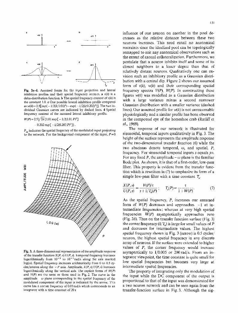
Fig. 2a-d. Assumed forms for the input projection and lateral inhibition profiles and their spatial frequency content, a v(k) is a delta-distribution function, b The spatial frequency content of v(k) is the constant 1.0. e One possible lateral inhibition profile computed as w(k)= 2.5[exp(- 1/2(k/1.O1) 2) -exp(- 1/2(k/0.202)2)]. The two in- dividual Gaussian curves are indicated by dashed lines, d Spatial frequency content of the assumed lateral inhibitory profile.

W(P) = 2 .51 /~{ 1.01 exp [ - 1/2(1.01 p)2]

- 0.202 exp [ - 1/2(0.202 p)2]/ .

Pin indicates the spatial frequency of the modulated input projecting to the network. For the background component of the input, P = 0

Fig. 3. A three-dimensional representation of the amplitude response of the transfer function X(P, s)/U(P, s). Temporal frequency increases logarithmically from 10 -a to 10+Srad/s along the axis marked log(o). Spatial frequency increases arithmetically from 0 to 0.5 cy- cles/neuron along the + P axis. Amplitude, X(P, s)/U(P, s) increases logarithmically along the vertical axis. The explicit forms of W(P) and V(P) are the same as those used in Fig. 2. The curve in the amplitude - co plane corresponding to the spatial frequency of the modulated component of the input is indicated by the arrow. This curve has a corner frequency of 0.05 rad/s which corresponds to an integrator with a time constant of 20 s

131

influence of one neuron on another in the pool de- creases as the relative distance between these two neurons increases. This need entail no anatomical restraints since the idealized pool can be topologically remapped to suit any anatomical observations such as the extent of axonal collateralization. Furthermore, we postulate that a neuron inhibits itself and some of its closest neighbors to a lesser degree than that of relatively distant neurons. Qualitatively one can en- vision such an inhibitory profile as a Gaussian distri- bution with a central dip. Figure 2 shows our assumed form of v(k), w(k) and their corresponding spatial frequency spectra V(P), W(P). In constructing these figures w(k) was modelled as a Gaussian distribution with a large variance minus a second narrower Gaussian distribution with a smaller variance (dashed lines). Our assumed profile for w(k) is not unreasonable physiologically and a similar profile has been observed in the compound eye of the horseshoe crab (Ratliff et al., 1969).

The response of our network is illustrated for sinusoidal, temporal inputs qualitatively in Fig. 3. The height of the surface represents the amplitude response of the two-dimensional transfer function (6) while the two abscissas denote temporal, co, and spatial, P, frequency. For sinusoidal temporal inputs s equals jco. For any fixed P, the amplitude - co plane is the familiar Bode plot. As shown, it is that of a first-order, low-pass filter. This property is evident from the transfer func- tion which is rewritten in (7) to emphasize its form of a simple low-pass filter with a time constant T,.

X(P, s) V(P)/r U(P, s) s + 1/Tn(P) ' T.(P) = 1 + W(P) (7)

As the spatial frequency, P, increases our assumed form of W(P) decreases and approaches - 1 at in- termediate frequencies; whereas at very high spatial frequencies W(P) asymptotically approaches zero (Fig. 2d). Thus on the transfer function surface (Fig. 3) the corner frequency (1/T,) is large for small values of P and decreases for intermediate values. The highest spatial frequency shown in Fig. 3 (arrow) is 0.5 cycles/ neuron, the highest spatial frequency in any discrete array of neurons. If the surface were extended to higher values of P, the corner frequency would increase asymptotically to 1/0.005 or 200 rad/s. From an in- tegrator viewpoint, the time constant is quite small for low spatial frequencies but becomes very large at intermediate spatial frequencies.

The property of integrating only the modulation of the input while the DC component of the output is proportional to that of the input was demonstrated for a two neuron network and can be seen again from the transfer-function surface in Fig. 3. Although the sig-

132

nals from push-pull, input structures are assumed to be interdigitated in space along the input to the network, the background component is the same for signals from the two sources. Thus P equals zero for the background component and, as Fig. 3 indicates, the output from this component has a high corner frequency; that is, it will not be integrated in the time domain. On the other hand, with the assumed in- terdigitated projections of the two inputs, the modu- lated component has a high, spatial-frequency content. If this P value is in the intermediate zone (Pi,, Fig. 2d) where W(P) is slightly more positive than - 1, then the amplitude response is large at low temporal frequen- cies and has a low corner frequency as shown in Fig. 3 by the arrow. Such a Bode plot is that of a leaky integrator with a long time constant. We shall assume that the spatial frequency of the input signal, P~,, is confined to this region.

One can note that in the region of spatial frequen- cies, P~,, where the network integrates best it is still necessary that W(P) be -0.99975. It would be im- possible to build an integrator with a 20 s time con- stant out of elements with 0.005s time constants without some global aspect of the network being held to a tight tolerance. We mean by robustness that the behavior of the model should not depend critically on any one connection or, in a model with thousands of connections, on even hundreds of connections. In particular, we consider the model robust if, in a given network, one can make significant alterations and lesions without losing the property of integration or becoming unstable. The proposed model does this as will be shown by a specific example in the next section.

In the continuum model considered here, this robustness can be seen by noting that W(P) is formed by many connections and would change very little if a few of them changed by large amounts or many by small amounts. We can, for example, simulate the latter by changing all the connections in a random way. Let w(k) be the sum of the ideal, deterministic inhibitory profile w(k) (Fig. 2c) plus some random noise n(k) which strengthens and weakens connections throughout the pool. Assume that n(k) has a band- limited, white-noise power spectrum, S,(P)

S,(p)={~o ]Pf <P* IP] > P*.

In a discrete model, P~, corresponds to the spatial frequency of every other neuron (0.5 cycles/neuron). If we prevent the noise from altering the strengths of connections alternately up and down the line (every other connection increased, every other decreased; at the spatial frequency Pin) we are, in effect, assuming that P* is less than Pi.. In that case the noise has no

effect on W(Pi. ) because Pi, is above the noise cut-off frequency. Consequently T, is unaffected by such noise. This means that T, is independent of random fluc- tuations in synaptic connections between neurons provided that the alterations not have the periodicity of the input itself. The robustness of the network with respect to this general form of noise is demonstrated numerically for a finite network simulation in the Discrete Realization section. Of course this form of noise will affect the transmittance of the background rate or DC component of the input to the network. However, with the parameter values listed in the legend of Fig. 2, when P equals zero, W(P) for the ideal deterministic case is 5.06 which is relatively large, so that even for a very liberal allowance of S,(0), T,(P) when P equals zero is orders of magnitude smaller than 20 s so that virtually none of the DC component will influence the integrated output of the network.

The time constant of the integrator is primarily a function of the area of the central notch of w(k). Recall that w(k) is constructed from the difference between two Gaussian distributions, one with a large variance minus a second with a smaller variance (Fig. 2c). The contribution to W(P) by the Gaussian with the larger variance approaches zero rapidly for increasing spatial frequencies. Therefore the value that W(P) approaches near Pi. in Fig. 2d is approximately proportional to the Gaussian component of w(k) with the smaller variance. In other words the value of W(Pin ) is related to an integral property of the central dip in w(k). Thus, while T, is not dependent on variations in general connectivity between more distant cells, and is still not dependent on variations in a few closer connections out of many, it is dependent on the average profile of close connections. From (6) it is evident that the model remains stable if and only if W(P) is greater than - 1. The value of W(P) as it approaches - 1 is also determined precisely by the area of the central dip in w(k). Thus by the same averaging argument just pre- sented, the stability of the model is also dependent on the average profile of close connections. One suspects that this average profile is maintained by some sort of parametric-adaptive control system (e.g. Optican and Robinson, 1980) that monitors T, and adjusts it. The most obvious way to detect changes in T, is to use the exquisite sensitivity of the visual system to detect leakiness; that is, central drift of the eye on eccentric gaze. From the above analysis, one way to then control T, is to modify, perhaps by a parallel circuit, the connectivity between cells and themselves and particu- larly their close neighbors. Again, any individual con- nection would be insignificant, only the overall result.

In order to adjust the background level and the integrator gains to realistic values, it is useful to have a mechanism for controlling them independently. The

133

background rates of vestibular afferents and central neurons carrying the eye-position signal are similar (about 100 spikes/s) so gain between the background rates of the input U(0, 0) and output X(0, 0) should be around 1.0. Since W(0) is 5.06, the DC gain from (6), 1/(I+W(0)), is 0.16. On the other hand, at P~,, (6) becomes approximately 1/(sz). Since v is 5ms, the integrator gain is 200. This is much too large since most brain-stem, oculomotor neurons have a gain around 2.0. The necessary gain changes can be effected by altering V(P). If v(k) is fit by a Gaussian curve, for example, instead of a delta function, it could have a value, V(0), near 6.06 for low spatial frequencies and a small value, e.g. 0.01, at high spatial frequencies such as p~,.z Thus, the gain of the integrator and the gain of the background can be adjusted independently.

5 Discrete Realization

While the previous section may help some to see the importance of spatial frequencies in the model - a concept perhaps unfamiliar to some oculomotor theoreticians - it hardly satisfies the more realistic neurophysiologist who wants to see, by specific exam- ple, what comes out for a given input and how sensitive that is to variations in the neural connections. Consequently randomness in w(k) and lesions in a portion of the network were simulated for a discrete model of 32 neurons. Thirty two, from experience, was felt to be a minimum required to simulate effects both near and relatively far from a lesion. Edge effects were eliminated by configuring the neurons in a circle so that neuron 32 was an immediate neighbor of neu- ron 1. Instead of performing matrix manipulations, we computed responses with the aid of an electrical- circuit, simulation package, SPICE, on a digital com- puter (Nagel, 1975). The net input to each neuron was computed according to (1) by a buffered voltage summer. The neuron was a low-pass, RC filter with a time constant of 5 ms, and the output of each neuron was also decoupled electrically from other loads. The frequency response for sinusoidal inputs and transient response for finite-duration, pulse inputs were com- puted. A variance of 1.5 was used for the wide Gaussian component of w(k) (see legend, Fig. 4), and the area of the dip in w(k) was chosen such that at P~, (0.5 cycles/neuron), T~(Pi~)=20s. This meant limiting self-inhibition so that w(0) was 0.00014. For simplicity we continued to use a delta function for v(k) even though this produces an integrator with a high gain. We felt that the added complexity in the simulation was not justified.

2 For example, if v(k) has the form 2.03 exp [ - 1/2(k/1.14)2], V(P) will produce the desired gains at P equal 0 and P equal P~,

8 . 8

8 .6

8 . 4

N e . 2

8

-(~.2

- 0 . 4

, I',~i !

,. ,~-, . . . . . . . . ,,-j,--"

I I 1 - 6 - 1 2 - 8 - 4

i

i 1 I J

0 4 8 12 6

k-kc,

Fig. 4. The deterministic lateral-inhibitory profile for a discrete network is shown as a solid line. The discrete values were computed as w(k)=exp [-1/2(k/1.5) 2] -0.99986 5(k) and these values are con- nected by straight line segments. The dashed lines illustrate three of the 32, discrete, independently-noisy distributions used to demon- strate robustness of the model with respect to band-limited spatial noise introduced in the inhibitory coefficients. For this distribution T~(0.5) was still 20 s

In the robustness argument for the continuous network, the noise was random, but all neurons had the same, (noisy), lateral-inhibitory profile. With the discrete model it is possible for each neuron to have independent, band-limited, random noise superim- posed on the deterministic value of its lateral- inhibitory profile. The band-limited noise was com- puted as a summation of the first six harmonics of the fundamental frequency of a 32 neuron network (0.031 cycles/neuron). Thus P*, the frequency band-limit for the noise is 0.19 cycles/neuron. The phase of each harmonic for a particular profile was randomly selec- ted from a uniform distribution in the interval [0, 2~] and the power of each harmonic was 0.5. In Fig. 4 three of the 32, noisy, inhibitory profiles (broken lines) are superimposed on an ideal deterministic profile (solid line) to illustrate the severity of the distortions introduced in w(k) by the noise. If all of the neurons were to have just one of these distorted profiles, then one could predict from the continuum analysis that T,(Pin ) would still be 20 s. However, if each neuron's profile is independently random, it is not as obvious intuitively that T,(Pin ) will be unaffected by the noise. Nevertheless a frequency response simulation of the model verified that T,(Pin ) is still 20 s for independent, randomly-distorted, inhibitory profiles while Tn(0 ) was 1.3ms. 3 Thus, even with grossly-distorted, lateral-

3 If there were a random, independent, DC component of the noise, then the background rate of each neuron would be different and depend on the particular form of the noise. However, the spatial DC component of the output (i.e. the equally-weighted mean over all the neurons) is still a first-order pole with a time constant of about 1.3 ms

134

8 0

6 0

~ 4 0

~ 2 0 <[

0

-20 "

2

1

CO G (w)

b

10

- 1

0 0 0.4 018 112 i6 210 214 2:g " TIME (sec)

Fig. 5a and b. Response to sinusoidal (a) and pulse (b) inputs of a 32-neuron discrete mode1 when one neuron has been destroyed, a Bode plot of the amplitude response for P = 0.5 cycles/neuron. The heavy solid line is the response of an equally weighted sum of the 16 neurons receiving an increase in the modulation of their input (the corresponding summed amplitude response for the other half of the network is identical). The dashed line represents the response of the intact model with a time constant of 20s. The light, continuous lines show examples of the input/output amplitude ratios for individual "neurons" and the curve number indicates distance (in neurons) away from the lesion, b Model response to a 50 ms pulse input of amplitude 1. The heavy, light, and dashed lines have the same meanings as in a

inhibitory profiles, the network still integrates the modulated component of its input well and inde- pendently of the background component.

A pathological lesion of the integrator pool was modelled by eliminating the lateral inhibition from one of the 32 neurons. This is equivalent to the cell death of 1/32 (3 %) of the integrator pool. This discontinuity in the network cuts a hole in the distribution w(k) over the missing neuron and this sharp spatial transient causes effects to be exerted at all spatial frequencies. Thus even at an input frequency P of 0.5 cycles/neuron, the response of all of the neurons is no longer identical. Therefore we must choose some measure of the re- sponse of the whole network to characterize the perfor- mance of the integrator. We used the simple assump- tion that the outputs from all of the neurons receiving inputs that modulate in the same direction are summed with equal weights. A similar summation for neurons that modulate in the opposite direction con- stituted a second output. The transfer function be- tween an input and its corresponding output is now no longer that of a simple first-order filter. The amplitude ratio of this input-output mapping is shown as a Bode plot in Fig. 5a and the transient response to a pulse with a duration of 50ms is shown in Fig. 5b. The response of the intact network that behaves like a simple first-order filter with a time constant of 20 s is shown by the dashed line for comparison. The summed output of the lesioned integrator is no longer a single exponential decay. Just after the pulse the response falls off rapidly, by about 15 % of the normal response

in this case, and then resumes a decay rate similar to the prelesion rate. The reason is easy to see. Cells adjacent to the lesion have lost much of their positive feedback through the lateral inhibitory pathways and they integrate very poorly (Fig. 5a and b, light lines). Cells further away leak less rapidly while cells quite far away are hardly affected. Thus the response in Fig. 5b (solid line) may be thought of as the sum of 16 leaky integrators all leaking at different rates. The response is obviously complicated but one can conceptually simplify it by regarding it as the sum of a small exponential with a short time constant (about 2s) and a larger one with a long, or normal, time constant. If a larger portion of the network were "lesioned", the initial decay would be larger and faster and the amplitude of the slower component would be less. Not surprisingly the background rates of cells near the lesioned cell are different from the group mean.

6 Discussion

The goal of this study is to propose a hypothetical network of neurons that operate in a linear range, consistent with observed, brain-stem, single-unit ac- tivity, and that function en m a s s e as a leaky integrator with a time constant on the order of 20s. As an improvement over previous models, we impose two further constraints on our network. First, it must be capable of integrating only that component of its input which encodes the motor command; that is, the modu-

135

lation superimposed on the background firing rate. Second, the network must be both stable and robust with respect to variability of the parameter values and the possibility of lesions within the network. Our analysis demonstrates that these goals are achieved by a lateral-inhibitory network of homogeneous neurons.

The lesion simulation suggests a mechanism for a variation of the common, clinical observation of gaze- evoked nystagmus. In this syndrome a patient's eyes drift centripetally on the attempt to maintain eccentric gaze, and at large angles of gaze corrective, rapid eye movements (saccades) are required repeatedly to re- capture the visual target. This produces a saw-toothed, jerky eye movement called nystagmus. If the integrator became leaky through a decrease in Tn, the eyes would, between saccades, drift toward the rest position (straight ahead) with a single exponential time course and this is often the case [see Robinson (1974) or Zee et al. (1981) for examples of experimentally-induced, gaze-evoked nystagmus]. In other cases, however, the eye begins to drift centrally rapidly but quickly slows down to a much slower rate. If the latter rate is consistent with a time constant of 10-20 s, it is barely discernable and the eye appears to come to rest. The puzzle has been, if the integrator is just leaky, why does the eye slip back only part way? Abel et al. (1978) proposed that the integrator should be divided into parts so that only part of it could be made leaky and we basically agree. Figure 5b shows that our model simulates this waveform nicely after a loss of one cell out of 32. The virtue of our model is that it is not necessary to decouple the integrator into separate parts (Abel et al., 1978) to get the result; the distributed model does this naturally since it permits the behavior of some cells (those near the lesion) to be quite different from others (those far away). Thus, this particular variety of gaze-evoked nystagmus is simulated well by partial lesions of our neural network.

Cerebellar lesions, especially of the flocculus, are known to decrease Tn from 20 to 1.3 s (Robinson, 1974; Zee et al., 1981) and it has been proposed that there exists a rather leaky integrator pool in the brain stem with the latter time constant and that some sort of feedback loop mainly through the flocculus, increases this time constant to 20 s. If this escalation were done by a lumped, positive feedback, the gain of that pathway would be 0.935 and would require that fluctuations be maintained within 7%o. This is not unreasonable, especially if this parameter is under feedback control, but it seems more likely to us that the transcerebellar pathway forms a parallel pathway by which brain-stem cells can influence their neigh- bors. By manipulating the distribution w(k), the time constant T, can easily be controlled in a way that does not depend on individual connections.

Because of midline symmetry, the neural integrator must consist of two groups of ceils, one in each half of the brain stem. Each could consist of inhibitory neu- rons driven in push-pull by Type I, excitatory, so- called pure-vestibular cells in the left and right vesti- bular nuclei. (A Type I neuron increases activity with ipsilateral head rotation ; a Type II neuron is just the opposite.) The activity of half the cells in each pool would increase while that of the other half would decrease. Thus the pool would be a mixture of Types I and II cells. Alternatively, all the cells driven from one vestibular input could be segregated on one side of the brain stem; their activity would all increase or decrease with increased activity of the vestibular input. This arrangement causes the two half integrators to operate in push-pull ; all the cells would be of the same type, I or II. They would be joined across the midline by lateral inhibitory connections.

Since Types I or II, excitatory or inhibitory vesti- bular neurons are abundant in the vestibular nuclei, there is no difficulty providing the vestibular inputs for either of these arrangements. Unfortunately, there is not enough physiological or anatomical data on cells that might be part of the integrator to form any opinion now about which arrangement might be more realistic; although, so far, no areas of the pons have been found that contain cells carrying the eye-position signal that are not mixed, some increasing their ac- tivity in one direction, others in the opposite direction. This tentative finding suggests the former rather than the latter alternative. The choices are not mutually exclusive and several or all could be operating at once. There are also double-layer models for neural net- works in which half the cells are excitatory, half inhibitory (Ermentrout et al., 1980). Such a model could also, no doubt, be made to integrate. A virtue of it would be that in coupling the integrator output to ocular motoneurons in a push-pull manner, that will also maintain a reasonable background rate on the latter, it is awkward if only inhibitory cells are avail- able and quite easy to do if both excitatory and inhibitory cells are available.

There are two quite unrealistic aspects of the cells in the model : they are all alike and they carry the eye- position signal but not a velocity signal. Neurons in the brain stem that carry the eye-position signal have a broad distribution of background rates and sensiti- vities to changes in eye position. Much of this in- homogeneity is probably brought to the pool on the vestibular input fibers themselves that also have a wide distribution of background rates and gains. Also, as the simulations with noisy connections and lesions show, these manipulations also create inhomogeneity in the pool. The missing velocity signal is a more serious problem. Cells without them are called pure-

136

tonic, or pure-position, and very few of them have been observed in the brain stem (Keller, 1974). Most cells also carry a signal proportional to eye velocity during vestibular, pursuit, or saccadic movements or some combination of them. Thus, the next step in making the model more realistic would be to find a way to make its cells respond to the modulated input itself as well as its integral.

Acknowledgements. The authors wish to thank A. McCracken for preparation of the manuscript and C. Bridges for drawing some of the figures. Computer graphics facilities and SPICE were provided by The Johns Hopkins University Engineering Computing Facility. S. Cannon was supported by grants GM07309 from the General Medical Institute and EY 07047 from the National Eye Institute of the National Institutes of Health (NIH), U.S. Public Health Service. D.A. Robinson received support from grant EY00598 from the National Eye Institute, NIH.

References

Abel, L.A., Dell'Osso, L.F., Daroff, R.B. : Analog model for gaze- evoked nystagmus. IEEE Trans. Biomed. Eng. 25:1, 71 75 (1978)

an der Heiden, U. : Analysis of neural networks. In : Lecture notes in biomathematics. Levin, S. (ed.), pp. 12-13. Berlin, Heidelberg, New York: Springer 1980

Becker, W., Klein, H. : Accuracy of saccadic eye movements and maintenance of eccentric eye positions in the dark. Vision Res. 13, 1021-1034 (1973)

Cohen, B., Komatsuzaki, A.: Eye movements induced by stimu- lation of the pontine reticular formation: evidence for in- tegration in oculomotor pathways: Exp. Neurol. 36, 101-117 (1972)

Doslak, M.J., Dell'Osso, L.F., Daroff, R.B. : A model of Alexander's law of vestibular nystagmus. Biol. Cybern. 34, 181-186 (1979)

Ermantrout, G.B., Cowan, J.D.: Large scale spatially organized activity in neural Nets. SIAM J. Applied Math. 38, 1-21 (1980)

Kamath, B.Y., Keller, E.L.: A neurological integrator for the ocutomotor control system. Math. Biosci. 30, 341-352 (1976)

Keller, E.L. : Participation of medial pontine reticular formation in eye movement generation in monkey. J. Neurophysiol. 37, 31 (~322 (1974)

Nagel, L.W.: SPICE 2: a computer to simulate semiconductor circuits, ERL Memo No. ERL-M520, Electronics Research Laboratory, Univ. of Calif., Berkeley (1975)

Optican, L.M., Robinson, D.A. : Cerebellar-dependent adaptive con- trol of primate saccadic system. J. Neurophysiol. 44, 1058-1076 (1980)

Rail, W. : Membrane potential transients and membrane time con- stants of motoneurons. Exp. Neurol. 2, 503-532 (1960)

Ratliff, K., Hartline, F. : Studies on excitation and inhibition in the retina. The Rockefeller University Press 1974

Ratliff, K., Knight, W.B., Graham, W. : On tuning and amplification by lateral inhibition. Proc. Natl. Acad. Sci. 62, 733-740 (1969)

Robinson, D.A.: Eye movement control in primates. Science 161, 1219-1224 (1968)

Robinson, D.A.: Models of oculomotor neural organization. In: The control of eye movements, Bach-y-Rita, P., Collins, C.C., Hyde, J.E. (eds.), pp. 51~538. New York: Academic Press 1971

Robinson, D.A. : The effect of cerebellectomy on the cat's vestibulo- ocular integrator. Brain Res. 71, 195-207 (1974)

Robinson, D.A. : Oculomotor control signals. In : Basic mechanisms of ocular motility and their clinical implications. Bach-y-Rita, P., Lennerstrand, G. (eds.), pp. 337-374. Oxford: Pergamon Press 1975 (Wenner-Gren Cent. Int. Symp. Ser.)

Rosen, MJ. : A theoretical neural integrator. IEEE Trans. Biomed. Eng. 19, 362-367 (1972)

Skavenski, A.A., Robinson, D.A.: Role of abducens neurons in vestibuloocular reflex. J. Neurophysiol. 36, 724-738 (1973)

van Gisbergen, J.A.M., Robinson, D.A., Gielen, S. : A quantitative analysis of the generation of saccadic eye movements by burst neurons. J. Neurophysiol. 45, 417-442 (1981)

Waespe, W., Henn, V. : Neuronal activity in the vestibular nuclei of the alert monkey during vestibular and optokinetic stimulation. Exp. Brain Res. 27, 523-538 (1977)

Zee, D.S., Friendlich, A.R., Robinson, D.A.: The mechanism of downbeat nystagmus. Arch. Neurol. 30, 227-237 (1974)

Zee, D.S., Yamazaki, A., Butler, P., Gucer, G. : Effect of ablation of flocculus and paraflocculus on eye movement in primate. J. Neurophysiol. 46, 878-899 (1981)

Received: September 13, 1983

Stephen C. Cannon Room 355 Woods Res. Bldg. The Wilmer Institute The Johns Hopkins Hospital 601 N. Broadway Baltimore, MD 21205 USA