A preliminary method for the evaluation of the landslides volume at a regional scale
13
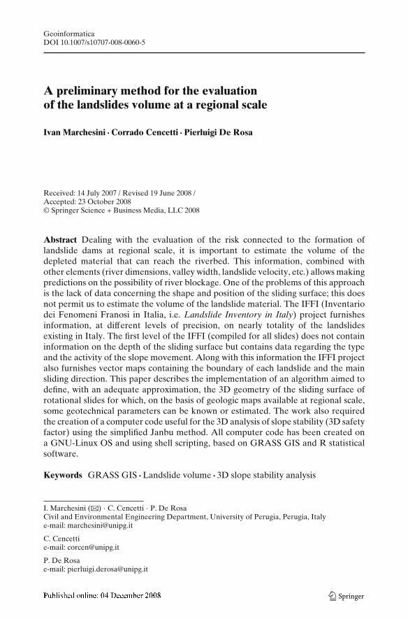
Geoinformatica DOI 10.1007/s10707-008-0060-5 A preliminary method for the evaluation of the landslides volume at a regional scale Ivan Marchesini · Corrado Cencetti · Pierluigi De Rosa Received: 14 July 2007 / Revised 19 June 2008 / Accepted: 23 October 2008 © Springer Science + Business Media, LLC 2008 Abstract Dealing with the evaluation of the risk connected to the formation of landslide dams at regional scale, it is important to estimate the volume of the depleted material that can reach the riverbed. This information, combined with other elements (river dimensions, valley width, landslide velocity, etc.) allows making predictions on the possibility of river blockage. One of the problems of this approach is the lack of data concerning the shape and position of the sliding surface; this does not permit us to estimate the volume of the landslide material. The IFFI (Inventario dei Fenomeni Franosi in Italia, i.e. Landslide Inventory in Italy) project furnishes information, at different levels of precision, on nearly totality of the landslides existing in Italy. The first level of the IFFI (compiled for all slides) does not contain information on the depth of the sliding surface but contains data regarding the type and the activity of the slope movement. Along with this information the IFFI project also furnishes vector maps containing the boundary of each landslide and the main sliding direction. This paper describes the implementation of an algorithm aimed to define, with an adequate approximation, the 3D geometry of the sliding surface of rotational slides for which, on the basis of geologic maps available at regional scale, some geotechnical parameters can be known or estimated. The work also required the creation of a computer code useful for the 3D analysis of slope stability (3D safety factor) using the simplified Janbu method. All computer code has been created on a GNU-Linux OS and using shell scripting, based on GRASS GIS and R statistical software. Keywords GRASS GIS · Landslide volume · 3D slope stability analysis I. Marchesini (B ) · C. Cencetti · P. De Rosa Civil and Environmental Engineering Department, University of Perugia, Perugia, Italy e-mail: [email protected] C. Cencetti e-mail: [email protected] P. De Rosa e-mail: [email protected]
Transcript of A preliminary method for the evaluation of the landslides volume at a regional scale
GeoinformaticaDOI 10.1007/s10707-008-0060-5
A preliminary method for the evaluationof the landslides volume at a regional scale
Ivan Marchesini · Corrado Cencetti · Pierluigi De Rosa
Received: 14 July 2007 / Revised 19 June 2008 /Accepted: 23 October 2008© Springer Science + Business Media, LLC 2008
Abstract Dealing with the evaluation of the risk connected to the formation oflandslide dams at regional scale, it is important to estimate the volume of thedepleted material that can reach the riverbed. This information, combined withother elements (river dimensions, valley width, landslide velocity, etc.) allows makingpredictions on the possibility of river blockage. One of the problems of this approachis the lack of data concerning the shape and position of the sliding surface; this doesnot permit us to estimate the volume of the landslide material. The IFFI (Inventariodei Fenomeni Franosi in Italia, i.e. Landslide Inventory in Italy) project furnishesinformation, at different levels of precision, on nearly totality of the landslidesexisting in Italy. The first level of the IFFI (compiled for all slides) does not containinformation on the depth of the sliding surface but contains data regarding the typeand the activity of the slope movement. Along with this information the IFFI projectalso furnishes vector maps containing the boundary of each landslide and the mainsliding direction. This paper describes the implementation of an algorithm aimed todefine, with an adequate approximation, the 3D geometry of the sliding surface ofrotational slides for which, on the basis of geologic maps available at regional scale,some geotechnical parameters can be known or estimated. The work also requiredthe creation of a computer code useful for the 3D analysis of slope stability (3D safetyfactor) using the simplified Janbu method. All computer code has been created ona GNU-Linux OS and using shell scripting, based on GRASS GIS and R statisticalsoftware.
Keywords GRASS GIS · Landslide volume · 3D slope stability analysis
I. Marchesini (B) · C. Cencetti · P. De RosaCivil and Environmental Engineering Department, University of Perugia, Perugia, Italye-mail: [email protected]
C. Cencettie-mail: [email protected]
P. De Rosae-mail: [email protected]
Geoinformatica
1 Introduction
1.1 The evaluation of sliding volume at a regional scale
The evaluation of landslide volume is strictly linked to slope stability analysis.Normally it is necessary to study in detail only a single landslide case, but it can alsohappen that it is necessary to evaluate the landslide volume at a regional scale. Inour case we had to estimate the volume at a regional scale for hundreds of landslidesin order to calculate the territorial vulnerability for landslide damming phenomena,that are linked to the volume of depleted material [3]. It was not necessary tohave an exact estimation of volume but just an estimate of order of magnitude.This estimation should be done iteratively for more than one hundred slides, sothe integration of this slope stability model into a Geographical Information System(GIS) allows us a simpler and more efficient analysis.
1.2 GIS approach to 3D stability analysis models
Trying to determine the sliding surface of a landslide is a hard task because eachlandslide is usually a complex combination of a lot of small movements. In orderto solve this problem many different modeling approaches have been used. Themajority of these models performs a two dimensional (2D) modeling of slopestability, using the limit equilibrium method within the domain of geotechnicalengineering. The safety factor is commonly assessed using a 2D representation ofthe slope.
While the results of the 2D analysis are usually conservative, 3D analysis tends toincrease the safety factor. The failure surface is assumed to be infinitely wide in 2Dmodeling, omitting the 3D effects. Some studies conclude that the 3D safety factoris usually greater than the corresponding 2D safety factor calculated for the mostcritical 2D [4].
Since the 1970s, the development of 3D stability models has attracted growinginterest, so the advent of a 3D approach for slope stability analysis has produced agreat number of computer programs. The most representative one is CLARA [6],which is commercially available, and can compute both 2D and 3D slope stabilityanalysis. TSLOPE3 [9] is another code that performs 3D slope stability analysisbut CLARA satisfies more equilibrium conditions using different methods of 3Danalysis.
The Geographical Information System (GIS), with capacities ranging from con-ventional data storage to complex spatial analysis, is becoming a powerful tool toimplement slope stability models. Since the usual slope stability models are ableto evaluate the sliding surface but cannot precisely place the sliding surface into ageographic reference system, the GIS approach can improve the analysis and theoverall usefulness of the obtained data.
3D analysis provides a better way to model slope stability than 2D analysis and aGIS approach allows the user to assess with precision the extent of the landslide andits position.
One of the first GIS approaches to slope stability analysis was performed by Xieet al. [11, 12] and was finalized to create the landslide susceptibility map of a region.
Geoinformatica
Recently the same authors improved their algorithm using the Monte Carlo methodto generate the centroids of the ellipsoids representing the sliding surfaces [13].
In this study, a 3D deterministic slope stability analysis is combined with a GISbased grid system to create a procedure useful to determine the volume of the slopemovements reported on a landslide inventory map. It was developed to work with alarge number of landslides (>1000) but, at the moment, it has been tested only overa small subset of them (we present the results from 5 landslides). Moreover a stand-alone procedure was created to perform a classical 3D stability analysis of a slope.Both procedures have been implemented using two free/open source softwares,GRASS GIS [5], [8] and R [10] running on a GNU-Linux OS (Debian Testing). Theinteroperability among three elements is guaranteed by the GNU-Linux Bash Shell.
The code is available under the terms of the GNU-GPL license at the website:http://www.unipg.it/~ivanm/scripts/.
2 The procedure to estimate landslide volume at regional scale
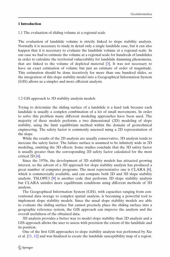
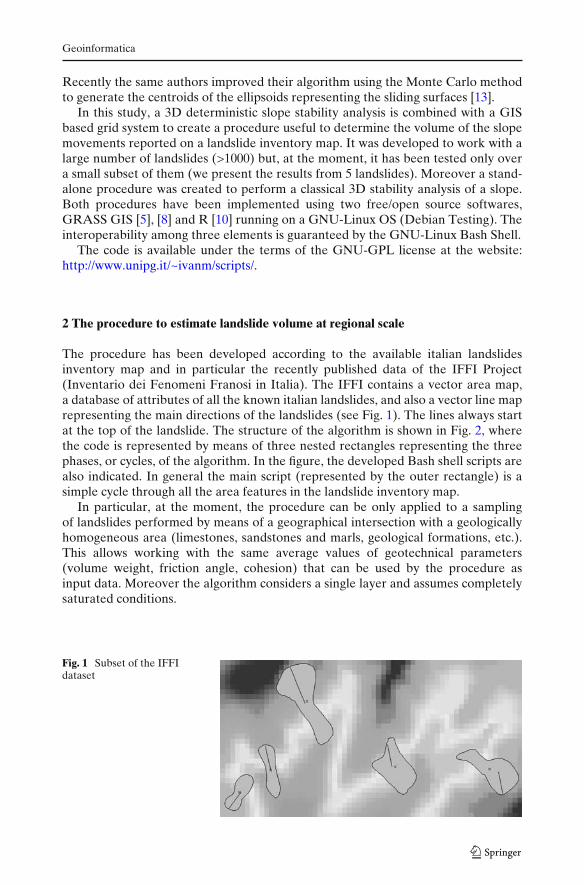
The procedure has been developed according to the available italian landslidesinventory map and in particular the recently published data of the IFFI Project(Inventario dei Fenomeni Franosi in Italia). The IFFI contains a vector area map,a database of attributes of all the known italian landslides, and also a vector line maprepresenting the main directions of the landslides (see Fig. 1). The lines always startat the top of the landslide. The structure of the algorithm is shown in Fig. 2, wherethe code is represented by means of three nested rectangles representing the threephases, or cycles, of the algorithm. In the figure, the developed Bash shell scripts arealso indicated. In general the main script (represented by the outer rectangle) is asimple cycle through all the area features in the landslide inventory map.
In particular, at the moment, the procedure can be only applied to a samplingof landslides performed by means of a geographical intersection with a geologicallyhomogeneous area (limestones, sandstones and marls, geological formations, etc.).This allows working with the same average values of geotechnical parameters(volume weight, friction angle, cohesion) that can be used by the procedure asinput data. Moreover the algorithm considers a single layer and assumes completelysaturated conditions.
Fig. 1 Subset of the IFFIdataset
Geoinformatica
Fig. 2 Procedure structure
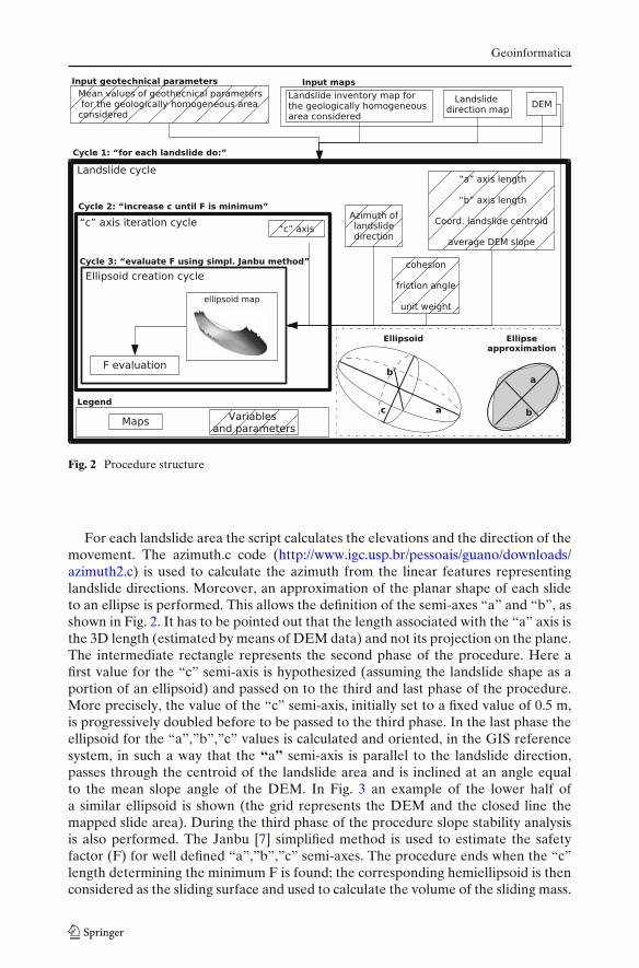
For each landslide area the script calculates the elevations and the direction of themovement. The azimuth.c code (http://www.igc.usp.br/pessoais/guano/downloads/azimuth2.c) is used to calculate the azimuth from the linear features representinglandslide directions. Moreover, an approximation of the planar shape of each slideto an ellipse is performed. This allows the definition of the semi-axes “a” and “b”, asshown in Fig. 2. It has to be pointed out that the length associated with the “a” axis isthe 3D length (estimated by means of DEM data) and not its projection on the plane.The intermediate rectangle represents the second phase of the procedure. Here afirst value for the “c” semi-axis is hypothesized (assuming the landslide shape as aportion of an ellipsoid) and passed on to the third and last phase of the procedure.More precisely, the value of the “c” semi-axis, initially set to a fixed value of 0.5 m,is progressively doubled before to be passed to the third phase. In the last phase theellipsoid for the “a”,”b”,”c” values is calculated and oriented, in the GIS referencesystem, in such a way that the “a” semi-axis is parallel to the landslide direction,passes through the centroid of the landslide area and is inclined at an angle equalto the mean slope angle of the DEM. In Fig. 3 an example of the lower half ofa similar ellipsoid is shown (the grid represents the DEM and the closed line themapped slide area). During the third phase of the procedure slope stability analysisis also performed. The Janbu [7] simplified method is used to estimate the safetyfactor (F) for well defined “a”,”b”,”c” semi-axes. The procedure ends when the “c”length determining the minimum F is found; the corresponding hemiellipsoid is thenconsidered as the sliding surface and used to calculate the volume of the sliding mass.
Geoinformatica
Fig. 3 Example of theellipsoidic sliding surface
In the following paragraphs some details regarding the implementation of theprocedure are given.
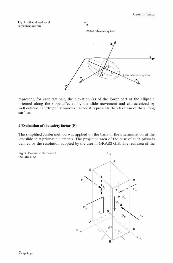
3 Ellipsoid creation and orientation
As already explained, the procedure assumes that the shape of the sliding surface canbe described by an hemiellipsoid. It is simple, inside the R workspace, to write thestandard equation describing an ellipsoid (local reference system).
x21
a2+ y2
1
b 2+ z2
1
c2= 1 (1)
The problem arises when we must describe the ellipsoid in a different referencesystem (global reference system), like the italian Gauss–Boaga Roma40 we wereworking with using GRASS GIS (Fig. 4). This task has been addressed, amongothers, by Xie et al. [12] with an equation that allows the expression of the threecoordinates of a point in a reference system (x1, y1, z1) by means of the coordinatesof the same point in another system (x,y,z):
⎡⎣
x1
y1
z1
⎤⎦ =
⎡⎣
a11 a12 a13
a21 a22 a23
a31 a32 a33
⎤⎦ x
⎡⎣
x − x0
y − y0
z − z0
⎤⎦ (2)
where
x0, y0, z0 are the known coordinates of the centroid of the landslide area,a11, a12, ....., anm are constants. The constants can be easily calculated and dependon the direction and inclination of the “a” axis.
Since the x,y coordinates where the ellipsoid must be calculated (i.e. the cellsbounded by the landslide perimeter) are known, it is possible to create an Rdataframe containing the pairs of these x,y values. This means that, for each celland from the equation of Xie et al. [12], one can express x1, y1, and z1 as a functionof z only.
Substituting such three new equations into the ellipsoid standard equation, asecond order equation in z may be obtained. The smallest values from this equation
Geoinformatica
Fig. 4 Global and localreference system
represent, for each x,y pair, the elevation (z) of the lower part of the ellipsoidoriented along the slope affected by the slide movement and characterized bywell defined “a”,”b”,”c” semi-axes. Hence it represents the elevation of the slidingsurface.
4 Evaluation of the safety factor (F)
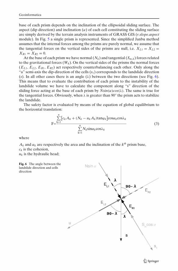
The simplified Janbu method was applied on the basis of the discrimination of thelandslide in n prismatic elements. The projected area of the base of each prism isdefined by the resolution adopted by the user in GRASS GIS. The real area of the
Fig. 5 Prismatic element ofthe landslide
Geoinformatica
base of each prism depends on the inclination of the ellipsoidal sliding surface. Theaspect (dip direction) and inclination (α) of each cell constituting the sliding surfaceare simply derived by the terrain analysis instruments of GRASS GIS (r.slope.aspectmodule). In Fig. 5 a single prism is represented. Since the simplified Janbu methodassumes that the internal forces among the prisms are purely normal, we assume thatthe tangential forces on the vertical sides of the prisms are null, i.e. XL1 = XL2 =XR1 = XR2 = 0.
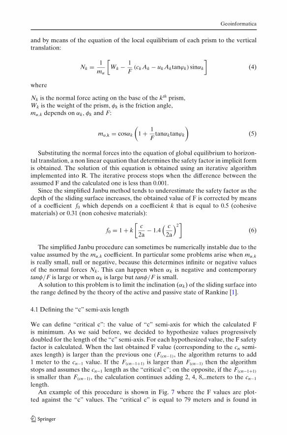
At the base of each prism we have normal (Nk) and tangential (Sm,k) forces relatedto the gravitational forces (Wk). On the vertical sides of the prisms the normal forces(EL1, EL2, ER1, ER2) act respectively counterbalancing each other. Only along the“a” semi-axis the dip-direction of the cells (s1) corresponds to the landslide direction(s). In all other cases there is an angle (λ) between the two directions (see Fig. 6).This means that to evaluate the contribution of each prism to the instability of thelandslide volume we have to calculate the component along “s” direction of thesliding force acting at the base of each prism by Nsin(α)cos(λ). The same is true forthe tangential forces. Obviously, when λ is greater than 90° the prism acts to stabilizethe landslide.
The safety factor is evaluated by means of the equation of global equilibrium tothe horizontal translation:
F=
n∑k=1
[ck Ah + (Nk − uk Ak)tanϕk
]cosαkcosλk
n∑k=1
Nksinαkcosλk
(3)
where
Ak and αk are respectively the area and the inclination of the kth prism base,ck is the cohesion,uk is the hydraulic head;
Fig. 6 The angle between thelandslide direction and cellsdirection
Geoinformatica
and by means of the equation of the local equilibrium of each prism to the verticaltranslation:
Nk = 1
mα
[Wk − 1
F(ck Ak − uk Aktanϕk) sinαk
](4)
where
Nk is the normal force acting on the base of the kth prism,Wk is the weight of the prism, φk is the friction angle,mα,k depends on αk, φk and F:
mα,k = cosαk
(1 + 1
Ftanαktanϕk
)(5)
Substituting the normal forces into the equation of global equilibrium to horizon-tal translation, a non linear equation that determines the safety factor in implicit formis obtained. The solution of this equation is obtained using an iterative algorithmimplemented into R. The iterative process stops when the difference between theassumed F and the calculated one is less than 0.001.
Since the simplified Janbu method tends to underestimate the safety factor as thedepth of the sliding surface increases, the obtained value of F is corrected by meansof a coefficient f0 which depends on a coefficient k that is equal to 0.5 (cohesivematerials) or 0.31 (non cohesive materials):
f0 = 1 + k[
c2a
− 1.4( c
2a
)2]
(6)
The simplified Janbu procedure can sometimes be numerically instable due to thevalue assumed by the mα,k coefficient. In particular some problems arise when mα,k
is really small, null or negative, because this determines infinite or negative valuesof the normal forces Nk. This can happen when αk is negative and contemporarytanφ/F is large or when αk is large but tanφ/F is small.
A solution to this problem is to limit the inclination (αk) of the sliding surface intothe range defined by the theory of the active and passive state of Rankine [1].
4.1 Defining the “c” semi-axis length
We can define “critical c”: the value of “c” semi-axis for which the calculated Fis minimum. As we said before, we decided to hypothesize values progressivelydoubled for the length of the “c” semi-axis. For each hypothesized value, the F safetyfactor is calculated. When the last obtained F value (corresponding to the cn semi-axes length) is larger than the previous one (F(cn−1), the algorithm returns to add1 meter to the cn−1 value. If the F(cn−1+1) is larger than F(cn−1) then the algorithmstops and assumes the cn−1 length as the “critical c”; on the opposite, if the F(cn−1+1)
is smaller than F(cn−1), the calculation continues adding 2, 4, 8,..meters to the cn−1
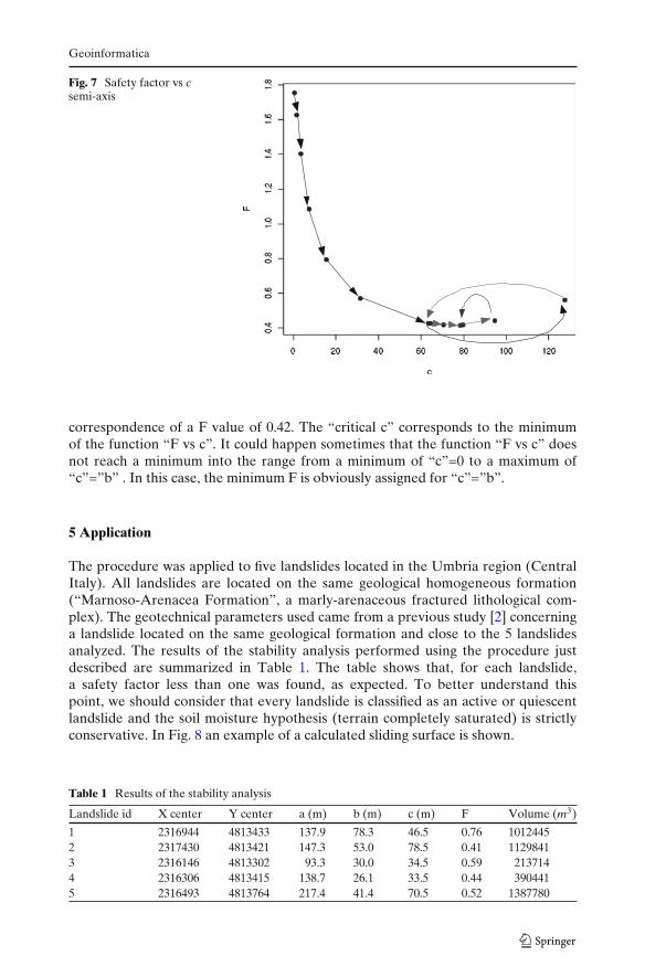
length.An example of this procedure is shown in Fig. 7 where the F values are plot-
ted against the “c” values. The “critical c” is equal to 79 meters and is found in
Geoinformatica
Fig. 7 Safety factor vs csemi-axis
correspondence of a F value of 0.42. The “critical c” corresponds to the minimumof the function “F vs c”. It could happen sometimes that the function “F vs c” doesnot reach a minimum into the range from a minimum of “c”=0 to a maximum of“c”=”b” . In this case, the minimum F is obviously assigned for “c”=”b”.
5 Application
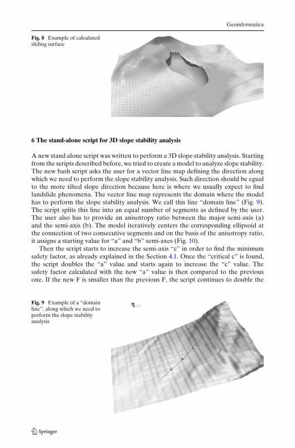
The procedure was applied to five landslides located in the Umbria region (CentralItaly). All landslides are located on the same geological homogeneous formation(“Marnoso-Arenacea Formation”, a marly-arenaceous fractured lithological com-plex). The geotechnical parameters used came from a previous study [2] concerninga landslide located on the same geological formation and close to the 5 landslidesanalyzed. The results of the stability analysis performed using the procedure justdescribed are summarized in Table 1. The table shows that, for each landslide,a safety factor less than one was found, as expected. To better understand thispoint, we should consider that every landslide is classified as an active or quiescentlandslide and the soil moisture hypothesis (terrain completely saturated) is strictlyconservative. In Fig. 8 an example of a calculated sliding surface is shown.
Table 1 Results of the stability analysis
Landslide id X center Y center a (m) b (m) c (m) F Volume (m3)
1 2316944 4813433 137.9 78.3 46.5 0.76 10124452 2317430 4813421 147.3 53.0 78.5 0.41 11298413 2316146 4813302 93.3 30.0 34.5 0.59 2137144 2316306 4813415 138.7 26.1 33.5 0.44 3904415 2316493 4813764 217.4 41.4 70.5 0.52 1387780
Geoinformatica
Fig. 8 Example of calculatedsliding surface
6 The stand-alone script for 3D slope stability analysis
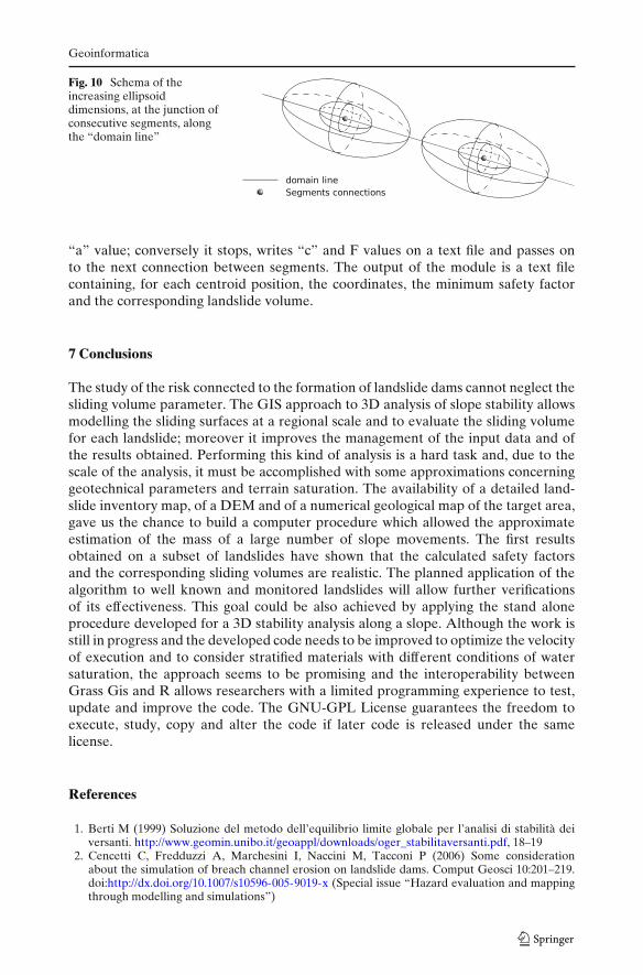
A new stand alone script was written to perform a 3D slope stability analysis. Startingfrom the scripts described before, we tried to create a model to analyze slope stability.The new bash script asks the user for a vector line map defining the direction alongwhich we need to perform the slope stability analysis. Such direction should be egualto the more tilted slope direction because here is where we usually expect to findlandslide phenomena. The vector line map represents the domain where the modelhas to perform the slope stability analysis. We call this line “domain line” (Fig. 9).The script splits this line into an equal number of segments as defined by the user.The user also has to provide an anisotropy ratio between the major semi-axis (a)and the semi-axis (b). The model iteratively centers the corresponding ellipsoid atthe connection of two consecutive segments and on the basis of the anisotropy ratio,it assigns a starting value for “a” and “b” semi-axes (Fig. 10).
Then the script starts to increase the semi-axis “c” in order to find the minimumsafety factor, as already explained in the Section 4.1. Once the “critical c” is found,the script doubles the “a” value and starts again to increase the “c” value. Thesafety factor calculated with the new “a” value is then compared to the previousone. If the new F is smaller than the previous F, the script continues to double the
Fig. 9 Example of a “domainline”, along which we need toperform the slope stabilityanalysis
Geoinformatica
Fig. 10 Schema of theincreasing ellipsoiddimensions, at the junction ofconsecutive segments, alongthe “domain line”
“a” value; conversely it stops, writes “c” and F values on a text file and passes onto the next connection between segments. The output of the module is a text filecontaining, for each centroid position, the coordinates, the minimum safety factorand the corresponding landslide volume.
7 Conclusions
The study of the risk connected to the formation of landslide dams cannot neglect thesliding volume parameter. The GIS approach to 3D analysis of slope stability allowsmodelling the sliding surfaces at a regional scale and to evaluate the sliding volumefor each landslide; moreover it improves the management of the input data and ofthe results obtained. Performing this kind of analysis is a hard task and, due to thescale of the analysis, it must be accomplished with some approximations concerninggeotechnical parameters and terrain saturation. The availability of a detailed land-slide inventory map, of a DEM and of a numerical geological map of the target area,gave us the chance to build a computer procedure which allowed the approximateestimation of the mass of a large number of slope movements. The first resultsobtained on a subset of landslides have shown that the calculated safety factorsand the corresponding sliding volumes are realistic. The planned application of thealgorithm to well known and monitored landslides will allow further verificationsof its effectiveness. This goal could be also achieved by applying the stand aloneprocedure developed for a 3D stability analysis along a slope. Although the work isstill in progress and the developed code needs to be improved to optimize the velocityof execution and to consider stratified materials with different conditions of watersaturation, the approach seems to be promising and the interoperability betweenGrass Gis and R allows researchers with a limited programming experience to test,update and improve the code. The GNU-GPL License guarantees the freedom toexecute, study, copy and alter the code if later code is released under the samelicense.
References
1. Berti M (1999) Soluzione del metodo dell’equilibrio limite globale per l’analisi di stabilità deiversanti. http://www.geomin.unibo.it/geoappl/downloads/oger_stabilitaversanti.pdf, 18–19
2. Cencetti C, Fredduzzi A, Marchesini I, Naccini M, Tacconi P (2006) Some considerationabout the simulation of breach channel erosion on landslide dams. Comput Geosci 10:201–219.doi:http://dx.doi.org/10.1007/s10596-005-9019-x (Special issue “Hazard evaluation and mappingthrough modelling and simulations”)
Geoinformatica
3. Costa JE, Schuster RL (1988) The formation and failure of natural dams. Geol Soc Amer Bull100:1054–1068
4. Duncan JM (1996) State of the art limit equilibrium and finite-element analysis of slopes.J Geotech Geoenviron Eng 7:577–596
5. GRASS Development Team (2008) Geographic resources analysis support system (GRASS)software, version 6.3.0. http://grass.osgeo.org
6. Hungr O (1998) CLARA: slope stability analysis in two or three dimensions. GeotechnicalResearch, West Vancouver
7. Janbu N, Bjerrum L, Kjaernsli B (1956) Soil mechanics applied to some engineering problems.Norwegian Geotechnical Institute, Oslo
8. Neteler M, Mitasova H (2007) Open source GIS: a GRASS GIS approach. Springer, New York9. Pyke R (1991) TSLOPE: users guide. Taga Engineering System and Software, Lafayette
10. R Development Core Team (2008) R: a language and environment for statistical computing.http://www.R-project.org
11. Xie M, Esaki T, Zhou G, Mitani Y (2003) Three-dimensional stability evaluation of land-slides and a sliding process simulation using a new geographic information systems component.Environ Geol 43:503–512
12. Xie M, Esaki T, Cai M (2004) A GIS-based method for locating the critical 3D slip surface in aslope. Comput Geotechnics 31:267–277
13. Xie M, Esaki T, Qiu C, Wang C (2006) Geographical information system-based computa-tional implementation and application of spatial three-dimensional slope stability analysis.Comput Geotechnics 33:260–274
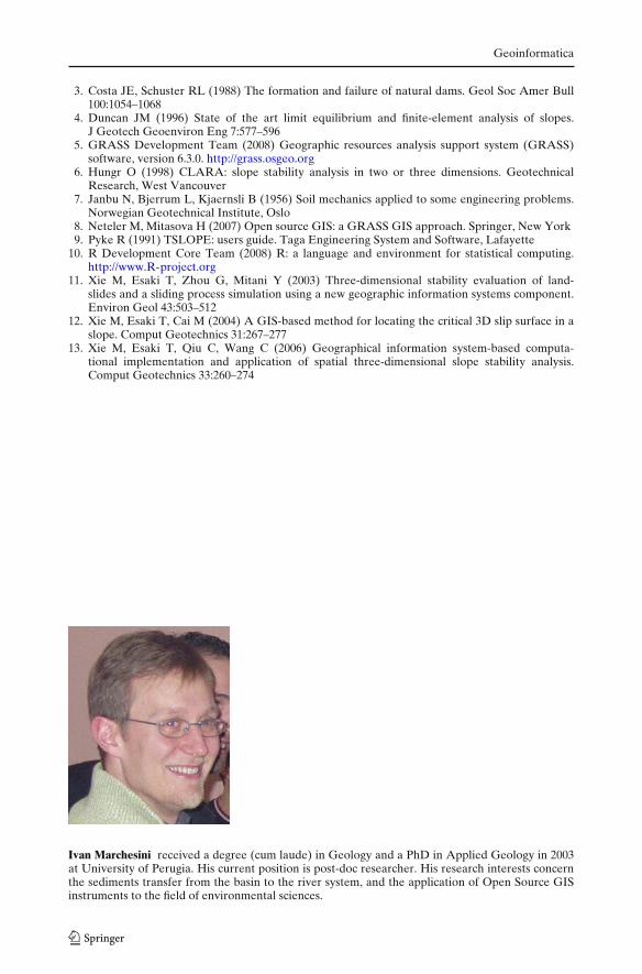
Ivan Marchesini received a degree (cum laude) in Geology and a PhD in Applied Geology in 2003at University of Perugia. His current position is post-doc researcher. His research interests concernthe sediments transfer from the basin to the river system, and the application of Open Source GISinstruments to the field of environmental sciences.
Geoinformatica
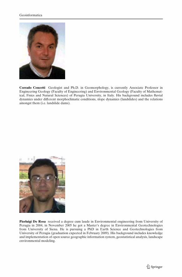
Corrado Cencetti Geologist and Ph.D. in Geomorphology, is currently Associate Professor inEngineering Geology (Faculty of Engineering) and Environmental Geology (Faculty of Mathemat-ical, Fisics and Natural Sciences) of Perugia University, in Italy. His background includes fluvialdynamics under different morphoclimatic conditions, slope dynamics (landslides) and the relationsamongst them (i.e. landslide dams).
Pierluigi De Rosa received a degree cum laude in Environmental engineering from University ofPerugia in 2004, in November 2005 he got a Master’s degree in Environmental Geotechnologiesfrom University of Siena. He is pursuing a PhD in Earth Science and Geotechnologies fromUniversity of Perugia (graduation expected in February 2009). His background includes knowledgeand implementation of open source geographic information system, geostatistical analysis, landscapeenvironmental modeling.