energies

Article

A Prediction Model of Pressure Loss of Cement Slurry inDeep-Water HTHP Directional Wells

Kunhong Lv 1, Hao Huang 1,*, Xingqiang Zhong 2, Yian Tong 3, Xingjie Ling 1 and Qiao Deng 1,*

�����������������

Citation: Lv, K.; Huang, H.; Zhong,

X.; Tong, Y.; Ling, X.; Deng, Q. A

Prediction Model of Pressure Loss of

Cement Slurry in Deep-Water HTHP

Directional Wells. Energies 2021, 14,

8180. https://doi.org/10.3390/

en14238180

Academic Editors: Reza Rezaee and

Riyaz Kharrat

Received: 10 October 2021

Accepted: 2 December 2021

Published: 6 December 2021

Publisher’s Note: MDPI stays neutral

with regard to jurisdictional claims in

published maps and institutional affil-

iations.

Copyright: © 2021 by the authors.

Licensee MDPI, Basel, Switzerland.

This article is an open access article

distributed under the terms and

conditions of the Creative Commons

Attribution (CC BY) license (https://

creativecommons.org/licenses/by/

4.0/).

1 College of Petroleum Engineering, Yangtze University, Wuhan 430199, China; lkhyxr@163.com (K.L.);lingxingjie2000@163.com (X.L.)

2 Zhanjiang Operation Company, CNOOC Petrochemicals Division, Zhanjiang 524000, China;zhongxingqiang168@163.com

3 Downhole Service Company, CNPC Chuanqing Drilling Engineering Co., Ltd., Chengdu 610052, China;tongzgsy@163.com

* Correspondence: 18772645696@163.com (H.H.); dengqiao@yangtzeu.edu.cn (Q.D.)

Abstract: The exploitations of deep-water wells often use directional well drilling to reach the targetlayer. Affected by special environments in deep water, the prediction of pressure loss of cementslurry is particularly important. This paper presents a prediction model of pressure loss suitable fordeep-water directional wells. This model takes the complex interaction between the temperature,pressure and hydration kinetics of cement slurry into account. Based on the initial and boundaryconditions, the finite difference method is used to discretize and calculate the model to ensure thestability and convergence of the result calculated by this model. Finally, the calculation equation ofthe model is used to predict the transient temperature and pressure loss of Wells X1 and X2, and acomparison is made between the predicted value and the monitoring data. The comparison resultsshow that the maximum error between the temperature and pressure predicted by the model and thefield measured value is within 6%. Thus, this model is of high accuracy and can meet the needs of siteconstruction. It is concluded that this result can provide reliable theoretical guidance for temperatureand pressure prediction, as well as the anti-channeling design of HTHP directional wells.

Keywords: deep water; directional wells; pressure loss; hydration reaction kinetics; temperature andpressure coupling; prediction model

1. Introduction

In recent years, the focus of oil–gas exploration and development has graduallyshifted from shallow-water areas to deep-water areas. Compared with land and shallowwater cementing, deep-water cementing operations are faced with the difficulties of hightemperature, high pressure and special environments, bringing great challenges to oil–gasexploration and development. The annular channeling formed in the cementing stagehas also become a problem to be solved urgently in the oil, natural gas and hydrateindustries [1,2]. During the waiting on cement stage, with the progression of the hydrationreaction, the gas will gradually enter the annulus space and cause gas channeling, whichoccurs when the liquid column pressure is lower than the formation pressure [3–6]. Atpresent, there are three mainstream views on the causes of annular channeling both athome and abroad. In the cementing process, the residual drilling fluid caused by lowdisplacement efficiency forms a channeling channel. During the waiting on cement stage, achanneling path is formed by formation fluid entering the annular gap when the annularliquid head is lower than the formation pressure due to the weight loss of cement slurry inthe waiting on cement (WOC) stage. After cement slurry solidification, a channeling pathis formed after the setting of cement slurry because of the poor cementing quality betweenthe cement sheath and borehole wall, as well as the casing. In the above three viewpoints,the weight loss of cement slurry in the WOC stage is the main cause of annular channeling.

Energies 2021, 14, 8180. https://doi.org/10.3390/en14238180 https://www.mdpi.com/journal/energies

Energies 2021, 14, 8180 2 of 15

Therefore, it is particularly important to carry out research on the prediction of the pressureloss pressure of cement slurry.

In the process of weight loss during the WOC stage, the continuous developmentof static gelling strength leads to insufficient pressure in the cement slurry column tostabilize the formation, which provides a driving force for the annular air channeling [7,8].Therefore, the establishment of an accurate temperature and pressure field calculationmodel and a pressure loss prediction model is a prerequisite for the safe and efficientcementing of high-temperature and high-pressure (HTHP) wells. Regarding this field ofresearch, there have already been some achievements. Carter et al. [9] believed that thebridge blinding caused by the gelatinization and filtration of cement slurry hindered theeffective transmission of the upper hydrostatic column pressure, which was an importantreason for the weight loss of cement slurry. Sabins et al. [10,11] first found that volumeshrinkage and gelatinization led to a decrease in liquid column pressure acting on thebottom of the well, resulting in the weight loss of cement slurry, and then put forward acorresponding theoretical model. Parcevaux et al. [12] proposed a relationship betweenpressure drop in the cement slurry column and gel strength, then provided a correspondingcorrelation. Sun [13] studied the pore pressure drops of three types of cement slurry due tosettling, settling–gelling (SG) weight loss and hydrated volume shrinking–gelling (HG)weight loss, then further analyzed the relationship between the three without filtration,revealing their internal mechanism and law. Zhang et al. [14–16] studied the importantinfluence of cement slurry’s stability on weight loss with a large number of weight lossexperiments based on the force analysis of cement slurry in the annulus. They also studiedthe quantitative relationship between effective slurry column pressure and gas cuttingresistance and the factors that affect the former two and set up a calculation model for theprocess of cement slurry setting, making the condition to cause breakthrough flow in theannulus, which can be used for predicting and evaluating the channeling preventing theability of cement slurry in the process of setting. Bu et al. [17] established a mechanicalmodel of the weight loss of cement slurry. They concluded that the weight loss of cementslurry is mainly related to the area of the annulus wall and the formation speed of cementslurry. Since the slurry temperature in the annulus varies with depth, the build-up of gelstrength and pressure drop are different at different depths, and the hydraulic pressureloss of the slurry column is calculated in sections. Li et al. [18] established an accuratecalculation model of hydraulic pressure loss of slurry and a developed sectional designand balanced cementing methods, which provided an effective calculation model for anti-gas channeling cementing design. Cheng et al. [19] investigated the evolution of cementslurry properties during liquid–solid transition by tests using X-ray diffraction (XRD),thermogravimetry (TG) and mechanical analysis and explained the causes of pressure lossin cement slurry from a microscopic point of view. Liu et al. [20] developed an apparatusfor evaluating the pressure loss of cement slurry at HTHP conditions by scaling down thesizes of existing apparatus. They carried out typical cement slurry weight loss pressureexperiments in vertical wells and inclined wells and proposed a piecewise calculationmethod of pressure loss, which has been tested in the field.

At present, the research of different scholars on the prediction model of pressureloss is mainly realized by the weight loss method and testing the change in static gellingstrength [21,22]. However, affected by the downhole complex environment and self-performance of cement slurry, it is difficult to accurately calculate the actual pressureloss merely based on existing models or experimental tests. In view of this, a model forcalculating the pressure loss in the WOC stage was derived in this research, taking intocomprehensive consideration the mutual action between the hydration reaction, tempera-ture and pressure of cement slurry, as well as the complicated deep-water environment.Finally, a comparison was made between the result measured on the site of Well X in ablock of a field, and the result was calculated on the basis of this model. The comparisonresult verifies the accuracy and stability of the model, which can provide more safe andeffective guidance for cementing construction.

Energies 2021, 14, 8180 3 of 15

2. Modeling2.1. Physical Model of Wellbore

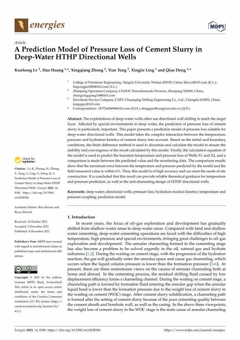
Most offshore oil–gas wells are directional wells with wellbore configuration [2]. Inthe process of cement injection, when cement slurry is displaced to the design depth ofthe annulus, it marks the completion of the injection and the starting of the WOC stage.For the HTHP well, during this stage, the cement slurry will undergo a violent hydrationreaction, with temperature and pressure varying with time and space change. The modelarea is divided into 3 blocks: formation, cement slurry in annular space and drilling fluidin the casing. The model is axisymmetric about the central axis of the wellbore (Figure 1).

Energies 2021, 14, x FOR PEER REVIEW 3 of 17

verifies the accuracy and stability of the model, which can provide more safe and effective guidance for cementing construction.

2. Modeling 2.1. Physical Model of Wellbore

Most offshore oil–gas wells are directional wells with wellbore configuration [2]. In the process of cement injection, when cement slurry is displaced to the design depth of the annulus, it marks the completion of the injection and the starting of the WOC stage. For the HTHP well, during this stage, the cement slurry will undergo a violent hydration reaction, with temperature and pressure varying with time and space change. The model area is divided into 3 blocks: formation, cement slurry in annular space and drilling fluid in the casing. The model is axisymmetric about the central axis of the wellbore (Figure 1).

Figure 1. Schematic diagram of the body structure of HTHP directional well.

2.2. Establishment for Wellbore Temperature Field Model 2.2.1. Fundamental Assumptions

When establishing the pressure loss calculation model, for the convenience of the research, the following hypotheses were made for the model: • Above the formation is a constant-temperature zone, which is homogeneously iso-

tropic with constant physical parameters; • The calculation satisfies Fourier’s law, and the geothermal gradient is known, not

considering heat source and fluid thermal convection, but only considering horizon-tal and vertical heat conduction;

• The heat convection in the wellbore is radial steady-state heat transfer, regardless of the axial temperature difference of the annular fluid;

• The physical parameters (such as density, specific heat capacity, thermal conductiv-ity, etc.) of each material in this model are always constant, which do not change with external factors. The specific heat and thermal conductivity are the same in the verti-cal and horizontal directions;

• Assuming that the drilling fluid and cement slurry do not mix with each other, they do not react with each other, and the interface is stable.

Figure 1. Schematic diagram of the body structure of HTHP directional well.

2.2. Establishment for Wellbore Temperature Field Model2.2.1. Fundamental Assumptions

When establishing the pressure loss calculation model, for the convenience of theresearch, the following hypotheses were made for the model:

• Above the formation is a constant-temperature zone, which is homogeneously isotropicwith constant physical parameters;

• The calculation satisfies Fourier’s law, and the geothermal gradient is known, notconsidering heat source and fluid thermal convection, but only considering horizontaland vertical heat conduction;

• The heat convection in the wellbore is radial steady-state heat transfer, regardless ofthe axial temperature difference of the annular fluid;

• The physical parameters (such as density, specific heat capacity, thermal conductivity,etc.) of each material in this model are always constant, which do not change withexternal factors. The specific heat and thermal conductivity are the same in the verticaland horizontal directions;

• Assuming that the drilling fluid and cement slurry do not mix with each other, theydo not react with each other, and the interface is stable.

Energies 2021, 14, 8180 4 of 15

2.2.2. Model Establishment

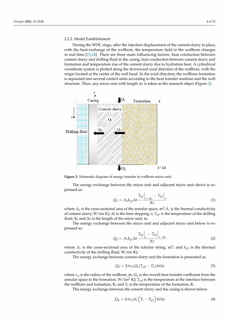
During the WOC stage, after the injection displacement of the cement slurry in place,with the heat exchange of the wellbore, the temperature field in the wellbore changesin real time [23,24]. There are three main influencing factors: heat conduction betweencement slurry and drilling fluid in the casing, heat conduction between cement slurry andformation and temperature rise of the cement slurry due to hydration heat. A cylindricalcoordinate system is plotted along the downward axial direction of the wellbore, with theorigin located at the center of the well head. In the axial direction, the wellbore formationis separated into several control units according to the heat transfer medium and the wellstructure. Then, any micro unit with length ∆z is taken as the research object (Figure 2).

Energies 2021, 14, x FOR PEER REVIEW 4 of 17

2.2.2. Model Establishment During the WOC stage, after the injection displacement of the cement slurry in place,

with the heat exchange of the wellbore, the temperature field in the wellbore changes in real time [23,24]. There are three main influencing factors: heat conduction between ce-ment slurry and drilling fluid in the casing, heat conduction between cement slurry and formation and temperature rise of the cement slurry due to hydration heat. A cylindrical coordinate system is plotted along the downward axial direction of the wellbore, with the origin located at the center of the well head. In the axial direction, the wellbore formation is separated into several control units according to the heat transfer medium and the well structure. Then, any micro unit with length zΔ is taken as the research object (Figure 2).

Figure 2. Schematic diagram of energy transfer in wellbore micro unit.

The energy exchange between the micro unit and adjacent micro unit above is ex-pressed as:

1df dfz z z

a df

T TQ A k t

z+Δ

−= Δ

Δ (1)

where aA is the cross-sectional area of the annular space, m2; ck is the thermal conduc-tivity of cement slurry, W/(m∙K); tΔ is the time stepping, s; dfT is the temperature of the drilling fluid, K; and zΔ is the length of the micro unit, m.

The energy exchange between the micro unit and adjacent micro unit below is ex-pressed as:

2df dfz z z

c df

T TQ A k t

z−Δ

−= Δ

Δ (2)

where cA is the cross-sectional area of the tubular string, m2; and dfk

is the thermal conductivity of the drilling fluid, W/(m∙K);

The energy exchange between cement slurry and the formation is presented as:

( )3 ,02 w e eQ r U T T t zαπ= − Δ Δ (3)

Figure 2. Schematic diagram of energy transfer in wellbore micro unit.

The energy exchange between the micro unit and adjacent micro unit above is ex-pressed as:

Q1 = Aakd f ∆tTd f

∣∣∣z+∆z

− Td f

∣∣∣z

∆z(1)

where Aa is the cross-sectional area of the annular space, m2; kc is the thermal conductivityof cement slurry, W/(m·K); ∆t is the time stepping, s; Td f is the temperature of the drillingfluid, K; and ∆z is the length of the micro unit, m.

The energy exchange between the micro unit and adjacent micro unit below is ex-pressed as:

Q2 = Ackd f ∆tTd f

∣∣∣z− Td f

∣∣∣z−∆z

∆z(2)

where Ac is the cross-sectional area of the tubular string, m2; and kd f is the thermalconductivity of the drilling fluid, W/(m·K);

The energy exchange between cement slurry and the formation is presented as:

Q3 = 2πrwUα(Te,0 − Te)∆t∆z (3)

where rw is the radius of the wellbore, m; Uα is the overall heat transfer coefficient from theannular space to the formation, W/(m2·K); Te,0 is the temperature at the interface betweenthe wellbore and formation, K; and Te is the temperature of the formation, K.

The energy exchange between the cement slurry and the casing is shown below:

Q4 = 2πrciUc

(Tc − Td f

)∆t∆z (4)

Energies 2021, 14, 8180 5 of 15

where rci is the inner diameter of the casing, m; Uc is the overall heat transfer coefficientfrom the casing to the annular space, W/(m2·K).

The energy gain and loss of the micro unit satisfies the law of conservation of energy.Based on this, the heat conduction model of the formation, the drilling fluid in the cas-ing and the cement slurry in the annulus and the corresponding difference form can beobtained:

The internal of formation: The heat transfer in formation satisfies the heat diffusionequation:

∂2Te

∂z2 +∂2Te

∂r2 +1r

∂Te

∂r=

ρece

ke

∂Te

∂t(5)

where ρe is the density of the formation, kg/m3; ce is the specific heat capacity of formation,J·kg−1·K−1; and ke is heat conductivity of the formation, W/(m2·K).

Heat conduction model of drilling fluid in the casing: The energy variation of themicro unit with length ∆z comes from the energy exchange of the adjacent micro unitsabove and below it and the heat exchange between the casing and the annular space. Theheat conduction model and the corresponding difference form are expressed as follows:(

Td f

∣∣∣t+∆t− Td f

∣∣∣t

)c f ρ f Ac∆z = 2πrciUc

(Tc − Td f

)∆t∆z−

Ackd f ∆tTd f |z− Td f |z−∆z

∆z + Ackd f ∆tTd f |z+∆z− Td f |z

∆z

(6)

Heat conduction model of cement slurry in the annular space: The energy change ofthe micro unit with length ∆z was derived from the energy exchange with the adjacentmicro units above and below it and the heat exchange between the casing and the annularspace, the heat conduction between the annular space and formation and the hydrationheat caused by cement slurry itself.

For the HTHP well, hydration heat of cement slurry is also a problem to consider, asit can lead to a temperature rise of the cement slurry and accelerate the hydration rate ofcement slurry. The heat released by cement slurry in the annular space can be calculatedon the basis of hydration kinetics:

Q =(

α|t+∆t − α)Qmaxρc Aa∆z (7)

According to the law of conservation of energy, and Equations (5)–(7), the heat transfermodel of cement slurry in the annular space can be expressed as:(

Tc|t+∆t − Tc|t)ccρc Aa∆z =

(α|t+∆t − α

)Qmaxρc Aa∆z

−2πrciUc

(Tc − Tf

)∆t∆z + 2πrwUa(Te,0 − Tc)∆t∆z

−Aakc∆t Tc |z− Tc |z−∆z∆z + Aakc∆t Tc |z+∆z− Tc |z

∆z

(8)

where Q is the hydration heat of cement slurry at any time, J/kg; α is the degree ofhydration of cement slurry; Qmax is the total heat released by hydration of cement slurry,J/kg; and ρc is the density of cement slurry, kg/m3.

Rewriting Equation (6) in differential form:

∂Tf

∂t=

2πrciUc

c f ρ f Ac

(Tc − Tf

)+

k f

c f ρ f

∂2Tf

∂z2 (9)

Combined with Equation (8), Equation (9) can be expressed as the following differenceform:

∂Tc

∂t=

2πrwUa

ccρc Aa(Te,0 − Tc)−

2πrciUc

ccρc Aa

(Tc − Tf

)+

Q∞

cc

∂α

∂t+

kc

ccρc

∂2Tc

∂z2 (10)

Energies 2021, 14, 8180 6 of 15

2.3. Establishment of Prediction Model of Pressure Loss of Cement Slurry

After cement slurry is in place, a spatial grid structure with certain strength is formedwith the passage of time. Meanwhile, due to the water loss and volume shrinkage ofcement slurry during solidification, the cement slurry column has a downward tendencyunder the action of its own weight and the pressure of the upper slurry column, formingthe overall cementing suspension weight loss effect of cement slurry. With the progressof the hydration reaction, the gel strength of cement slurry increases gradually, and thecementing suspension capacity of the grid structure becomes stronger, sharing partialhydrostatic fluid column pressure. Consequently, a constant reduction was seen in theeffective pressure of the cement slurry column [25].

During the solidification of cement slurry, for the selected cement slurry cells in thegrid structure, the cement slurry’s column pressure is:

Pe = ρcg∆z− 4τs∆zDw − Dco

(11)

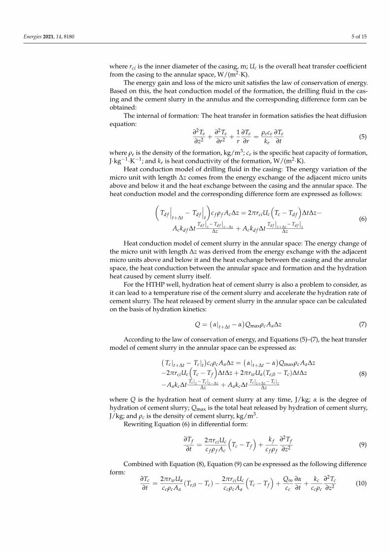
where Pe is the cement slurry’s column pressure, Pa.Moore et al. [26] proposed an overall cementing suspension weight loss effect of

cement slurry on the basis of the classical shear stress model. For directional well, theforces on the model will change. In this model, the cement slurry unit is subjected to fiveforces (Figure 3):

Energies 2021, 14, x FOR PEER REVIEW 7 of 17

Figure 3. Schematic diagram of forces of the cement slurry micro unit.

The downward force from the upper slurry column:

( )2 21

1 4w coP D D

Fπ× −

= (12)

The upward force from the lower slurry column:

( )2 22

2 4w coP D D

Fπ× −

= (13)

Gravity of cell itself:

( )2 2

4w coD D z

Gπ γ− Δ

= (14)

where γ is the volumetric weight of cement slurry, M/m3; Due to the gelling suspension effect, the cement slurry is subjected to the upward

cementing suspension force from the shaft wall and the casing:

( )s w coF D D zτ π= × + × Δ (15)

Holding power N perpendicular to the surface of the annular space: For the cement slurry cell, to meet the force balance, the axial and vertical forces of

the cement slurry on the wellbore satisfied the following equation:

( )2 1cos 0G F F Fα− − − = (16)

( )2 sin 0G F Nα− − = (17)

The effective slurry column pressure at the WOC stage of the cement slurry can be obtained as:

4cos se

w co

zP zD D

τγ α Δ= Δ −−

(18)

Figure 3. Schematic diagram of forces of the cement slurry micro unit.

The downward force from the upper slurry column:

F1 =P1 × π

(D2

w − D2co)

4(12)

The upward force from the lower slurry column:

F2 =P2 × π

(D2

w − D2co)

4(13)

Energies 2021, 14, 8180 7 of 15

Gravity of cell itself:

G =π(

D2w − D2

co)γ∆z

4(14)

where γ is the volumetric weight of cement slurry, M/m3;Due to the gelling suspension effect, the cement slurry is subjected to the upward

cementing suspension force from the shaft wall and the casing:

F = τs × π(Dw + Dco)× ∆z (15)

Holding power N perpendicular to the surface of the annular space:For the cement slurry cell, to meet the force balance, the axial and vertical forces of the

cement slurry on the wellbore satisfied the following equation:

(G− F2) cos α− F1 − F = 0 (16)

(G− F2) sin α− N = 0 (17)

The effective slurry column pressure at the WOC stage of the cement slurry can beobtained as:

Pe = γ∆z cos α− 4τs∆zDw − Dco

(18)

The corresponding pressure loss could be expressed as:

∆p =4τs∆z

Dw − Dco(19)

where ∆p is the pressure loss, Pa; τs is the static gelling strength of cement slurry, Pa; Dw isthe diameter of wellbore, m; and Dco is the outer diameter of the casing, m.

In the process of cementing, the pressure loss at different depths and moments couldbe calculated as the following equation:

∂p∂z

= max{

4τs

Dw − Dco, ρwg

}(20)

where ρw is the density of pore water, kg/m3.

2.4. Hydration Kinetic Model of Cement Slurry

Hydration kinetics is a method for dynamic research on the hydration reaction basedon its internal influence factor (the structure of cement slurry) and external influence factor(the reaction conditions), which can dynamically simulate and depict the hydration processso as to reveal the macro and internal mechanisms of the hydration reaction. For hydrationkinetics, the hydration kinetic model of cement-based materials proposed by Krstulovicet al. [25] is widely recognized. In this model, the hydration reaction of cement slurry isdivided into three processes: nucleation and crystal growth (NG), interactions at the phaseboundaries (I) and diffusion (D). The kinetic equations between hydration degree and thereaction time of the three processes and their corresponding differential forms are shownin Equations (21)–(23):

NG Process: {[− ln(1− α)]

1n = KNG(t− t0)

dαdt = KNGn(1− α)[− ln(1− α)]

n−1n

(21)

I Process: [1− (1− α)

13]1

= KI(t− t0)

dαdt = 3KI(1− α)

23

(22)

Energies 2021, 14, 8180 8 of 15

D Process: [1− (1− α)

13]2

= KD(t− t0)

dαdt = 3KD(1−α)

23

2[

1−(1−α)13

] (23)

where n is the order of chemical reactions; KNG is the reaction rate constant for the processof nucleation and crystal growth, s−1; KI is the reaction rate constant for the process ofinteractions at the phase boundaries, s−1; KD is the reaction rate constant for the process ofdiffusion, s−1; and t0 is the terminal stage of the induction period, s.

Isothermal calorimetry can be used to obtain the relationship between the heat releaserate dQ/dt, heat release amount Q and time t of the hydration. The hydration degree isusually described by hydration heat and other parameters easy to quantify. The relationshipbetween hydration degree and hydration time is presented as follows:

α = Q(t)/Qmax (24)

dα

dt=

dQ/dtQmax

(25)

where t is the hydration reaction time of cement slurry, s; Q(t) is the heat released by thehydration of cement slurry over time, J/kg; and α is the hydration degree of cement slurry.

Chemical reaction rate is significantly affected by temperature. Generally, the hydra-tion rates of cement slurry are higher at higher temperatures. However, for the HTHPwell, the wellbore at different depth experiences different temperatures and hydrationrates. According to reference [27], the impact of temperature on the chemical reaction rateconstant can be expressed by the Arrhenius equation:

K = K0e−Ea/RT (26)

where K is the reaction rate constant, s−1; K0 is the prefactor, also called frequency fac-tor, s−1; Ea is the activation energy of the reactant, J·mol−1; R is the ideal gas constant,J·K−1·mol−1; and T is the thermodynamic temperature, K.

The progress of the chemical reaction is mainly changed by the impact of temperaturefield and pressure field on the chemical reaction rate constant. Combined with Equation (9),the relation between chemical reaction rate and temperature and pressure is reflected asfollows [28]:

K = Kre−Ea/RT[

Ea

R

(1Tr− 1

T

)+

∆VR

(pr

Tr− p

T

)](27)

where Kr is the chemical reaction rate constant at the reference temperature and pressure,s−1; Tr is the reference temperature of the chemical reaction, K; T is the temperature of thechemical reaction, K; pr is the reference pressure of the chemical reaction, Pa; and p is thepore pressure of cement slurry, Pa.

3. Calculation of the Model

In the cementing process of the HTHP well, the hydration heat has a large influenceon the temperature and pressure, and there is also a mutual influence between the tem-perature and pressure. Therefore, when studying the pressure loss in the WOC stage, thetemperature field, pressure field and the hydration kinetic model of cement slurry arecoupled by the finite difference method to calculate the model.

3.1. Initial and Boundary Conditions

The following initial and boundary conditions are provided for calculation of themodel established in this paper:

1. Initial conditions:

Energies 2021, 14, 8180 9 of 15

Before the initial hydration, the cement slurry enters the annular space between thecasing and the wellbore. The initial condition of the waiting cement slurry is the tempera-ture of the cement slurry at the end of the injection displacement cycle, which is calculatedby using the circulating temperature prediction model stated in References [29,30]:

1v f

∂Tf

∂t+

∂Tf

∂z=

2πrciUc

c f w f

(Tc − Tf

)(28)

1vc

∂Tc

∂t− ∂Tc

∂z=

2πrwUc

ccwc(Te,0 − Tc)−

2πrciUc

ccwc

(Tc − Tf

)(29)

where w f = Acv f ρ f is the mass flow rate of drilling fluid in the casing, kg/s; wc is themass flow rate of cement slurry in the annular space, kg/s; Ac is the cross-sectional area ofcasing, m2; and v f is the circulating velocity of drilling fluid in casing, m/s.

The temperature of the constant-temperature layer is known. As the depth increases,the ground temperature increases linearly in depth and can be calculated on the basis ofthe geothermal gradient:

Te(r → ∞, z, t) = zge cos θ + Tconst (30)

where g f is the geothermal gradient, ◦C/100 m; θ is the deviation angle, ◦; and Tcont is theland surface temperature, ◦C.

The initial hydration degree of cement slurry is zero:

α|t=0 = 0 (31)

According to the hydrostatic fluid column pressure of cement slurry, the initial pres-sure of cement slurry can be calculated:

p(z)|t=0 = ρcgz (32)

2. Boundary conditions:

Infinitely away from the borehole, the formation temperature is the original statictemperature of the formation:

∂Te(r, z, t)∂r

∣∣∣∣r→∞

= 0 (33)

Because of the axisymmetric calculational domain, the borehole center satisfies theadiabatic condition:

∂T∂r

∣∣∣∣r=0

= 0 (34)

The annular temperature and casing temperature in the bottom of the well are identi-cal:

Tc(z = H, t) = Tf (z = H, t) (35)

The pore pressure of cement slurry at the wellhead position is environmental pressure:

p0 = pen (36)

The formation temperature is the undisturbed ground temperature at a certain distancebelow the well bottom:

Te(r, zd + z′, t

)= Tconst + tg

(zd + z′

)(37)

The heat transfer at the wellbore-formation interface can be expressed as:

∂Tb∂t

ρece =Tc − Tb

rwUa +

∂Tbr∂r

ke (38)

Energies 2021, 14, 8180 10 of 15

where Tb is the wellbore-formation interface temperature, ◦C.

3.2. Grid Division

Considering that the borehole diameter is much smaller than the length of the wellbore,the model is designed axisymmetric to the center axis of the wellbore in the direction of theborehole diameter.

3.3. Discrete Calculation of the Model

In the process of calculating the model, considering the coupling effect of variousfactors, the above partial differential equations are transformed into finite difference formby using the finite difference technology of the grid unit on the basis of the above-calculatedgrid unit in order to improve the calculation accuracy and efficiency:

T(m+1)c,i = T(m)

c,i −2πrciUc∆t

ccρc Aa

[T(m)

c,i = T(m)f ,i

]+ 2πrwUa∆t

ccρc Aa

[T(m)

i,0 = T(m)c,i

]+Q∞

cc

[α(m+1)i − α

(m)i

]+ kc∆t

ccρc

T(m)c,i+1−2T(m)

c,i+1+T(m)c,i−1

∆z2

(39)

p(m+1)i = p(m+1)

i−1 + max{

4τs∆zDw − Dco

, ρwg∆z}

(40)

α(m+1)i = α

(m)i + KNGn

[1− α

(m)i

]{− ln

[1− α

(m)i

]} n−1n ∆t (41)

α(m+1)i = α

(m)i + 3K1

[1− α

(m)i

]∆t (42)

α(m+1)i = α

(m)i +

32

KD

[1− α

(m)i

] 23{

1−[1− α

(m)i

] 13}

∆t(43)

where M is the last node in the horizontal direction; N is the node at the position at thebottom of the well; n is the order of chemical reactions; m is the time node; i is the spacenode in the vertical direction; and j is the space node in the horizontal direction.

3.4. Coupling Solution Method

In order to obtain the wellbore temperature and pressure of the HTHP directional well,it is necessary to use the iterative method for calculation. The concrete solving method is asfollows: input basic parameters, initial conditions and boundary conditions; mesh radiallyand axially (Figure 4) and define initial nodes and step sizes; according to the currentinitial conditions, the temperature, pressure and hydration dynamics parameters at nodei are calculated and updated; according to the hydration kinetics model, the hydrationkinetics parameters of cement slurry at node i are calculated; combined with the establishedtemperature field model, the transient temperature of node i is calculated; combined withthe established pressure field model, the transient pressure of node i is calculated; thetemperature and pressure calculation results are checked as per the test data to see whetherthey reach the required accuracy or not. If not, the calculation should be restarted fromStep (3); if yes, the calculation is ended, and the calculation of the next time node is started;output the result.

In order to clearly express the coupled iterative calculation process, a calculationflowchart is drawn (Figure 5).

Energies 2021, 14, 8180 11 of 15

Energies 2021, 14, x FOR PEER REVIEW 12 of 17

method is as follows: input basic parameters, initial conditions and boundary conditions; mesh radially and axially (Figure 4) and define initial nodes and step sizes; according to the current initial conditions, the temperature, pressure and hydration dynamics param-eters at node i are calculated and updated; according to the hydration kinetics model, the hydration kinetics parameters of cement slurry at node i are calculated; combined with the established temperature field model, the transient temperature of node i is cal-culated; combined with the established pressure field model, the transient pressure of node i is calculated; the temperature and pressure calculation results are checked as per the test data to see whether they reach the required accuracy or not. If not, the calculation should be restarted from Step (3); if yes, the calculation is ended, and the calculation of the next time node is started; output the result.

Figure 4. Schematic diagram of grid division.

In order to clearly express the coupled iterative calculation process, a calculation flowchart is drawn (Figure 5).

Figure 4. Schematic diagram of grid division.

Energies 2021, 14, x FOR PEER REVIEW 13 of 17

Figure 5. Calculation flowchart of the pressure loss prediction model.

4. Case Analysis There is a block with 90 m in water depth, 4000–4200 m in buried depth of the reser-

voir, about 2.30 in pressure coefficient of the reservoir and 195–215 °C in the reservoir temperature, belonging to a typical HTHP gas field. In order to verify the reliability of the model established in this research, a case analysis was carried out on Wells X1 and X2 in this block. The basic parameters and physical parameters of this well are illustrated in Tables 1 and 2.

Table 1. Basic parameters of Well X1.

Parameter Value Parameter Value Well type Directional well Thermal conductivity of formation (W∙m−1∙K−1) 2.03

Well depth (m) 5150 Thermal conductivity of cement (W∙m−1∙K−1) 1.03 Water depth (m) 90 Thermal conductivity of drilling fluid (W∙m−1∙K−1) 0.83

Lowering depth of casing (m) 5145 Thermal conductivity of casing (W/m∙K) 48.37 Kick off point (m) 4350 Density of formation (kg∙m−3) 2241.7

Well diameter (mm) 212.725 Density of drilling fluid (kg∙m−3) 2320 Outer diameter of casing (mm) 177.8 Density of cement slurry (kg∙m−3) 2400 Inner diameter of casing (mm) 152.5 Specific heat capacity of drilling fluid (J∙kg−1∙K−1) 1600 Temperature at mud line (°C) 10 Specific heat capacity of cement slurry (J∙kg−1∙K−1) 1840

Geothermal gradient (°C 100 m−1) 4 Specific heat capacity of formation (J∙kg−1∙K−1) 840

Figure 5. Calculation flowchart of the pressure loss prediction model.

4. Case Analysis

There is a block with 90 m in water depth, 4000–4200 m in buried depth of thereservoir, about 2.30 in pressure coefficient of the reservoir and 195–215 ◦C in the reservoirtemperature, belonging to a typical HTHP gas field. In order to verify the reliability ofthe model established in this research, a case analysis was carried out on Wells X1 and X2

Energies 2021, 14, 8180 12 of 15

in this block. The basic parameters and physical parameters of this well are illustrated inTables 1 and 2.

Table 1. Basic parameters of Well X1.

Parameter Value Parameter Value

Well type Directional well Thermal conductivity of formation (W·m−1·K−1) 2.03Well depth (m) 5150 Thermal conductivity of cement (W·m−1·K−1) 1.03

Water depth (m) 90 Thermal conductivity of drilling fluid (W·m−1·K−1) 0.83Lowering depth of casing (m) 5145 Thermal conductivity of casing (W/m·K) 48.37

Kick off point (m) 4350 Density of formation (kg·m−3) 2241.7Well diameter (mm) 212.725 Density of drilling fluid (kg·m−3) 2320

Outer diameter of casing (mm) 177.8 Density of cement slurry (kg·m−3) 2400Inner diameter of casing (mm) 152.5 Specific heat capacity of drilling fluid (J·kg−1·K−1) 1600Temperature at mud line (◦C) 10 Specific heat capacity of cement slurry (J·kg−1·K−1) 1840

Geothermal gradient (◦C 100 m−1) 4 Specific heat capacity of formation (J·kg−1·K−1) 840

Table 2. Basic parameters of Well X2.

Parameter Value Parameter Value

Well type Directional well Thermal conductivity of formation (W·m−1·K−1) 2.03Well depth (m) 5570 Thermal conductivity of cement (W·m−1·K−1) 1.03

Water depth (m) 90 Thermal conductivity of drilling fluid (W·m−1·K−1) 0.83Lowering depth of casing (m) 5560 Thermal conductivity of casing (W/m·K) 48.37

Kick off point (m) 4600 Density of formation (kg·m−3) 2241.7Well diameter (mm) 212.725 Density of drilling fluid (kg·m−3) 2370

Outer diameter of casing (mm) 177.8 Density of cement slurry (kg·m−3) 2400Inner diameter of casing (mm) 152.5 Specific heat capacity of drilling fluid (J·kg−1·K−1) 1610Temperature at mud line (◦C) 10 Specific heat capacity of cement slurry (J·kg−1·K−1) 1840

Geothermal gradient (◦C 100 m−1) 4 Specific heat capacity of formation (J·kg−1·K−1) 840

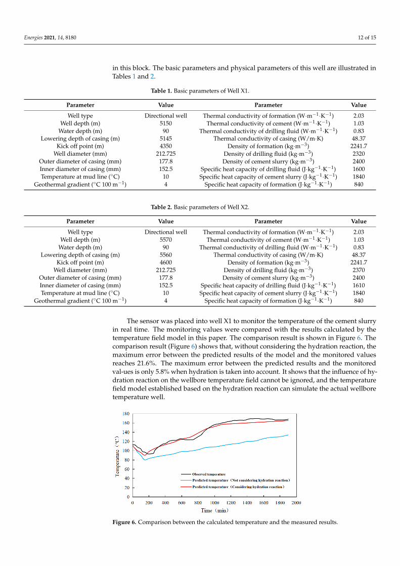
The sensor was placed into well X1 to monitor the temperature of the cement slurryin real time. The monitoring values were compared with the results calculated by thetemperature field model in this paper. The comparison result is shown in Figure 6. Thecomparison result (Figure 6) shows that, without considering the hydration reaction, themaximum error between the predicted results of the model and the monitored valuesreaches 21.6%. The maximum error between the predicted results and the monitoredval-ues is only 5.8% when hydration is taken into account. It shows that the influence of hy-dration reaction on the wellbore temperature field cannot be ignored, and the temperaturefield model established based on the hydration reaction can simulate the actual wellboretemperature well.

Energies 2021, 14, x FOR PEER REVIEW 14 of 17

Table 2. Basic parameters of Well X2.

Parameter Value Parameter Value Well type Directional well Thermal conductivity of formation (W∙m−1∙K−1) 2.03

Well depth (m) 5570 Thermal conductivity of cement (W∙m−1∙K−1) 1.03 Water depth (m) 90 Thermal conductivity of drilling fluid (W∙m−1∙K−1) 0.83

Lowering depth of casing (m) 5560 Thermal conductivity of casing (W/m∙K) 48.37 Kick off point (m) 4600 Density of formation (kg∙m−3) 2241.7

Well diameter (mm) 212.725 Density of drilling fluid (kg∙m−3) 2370 Outer diameter of casing (mm) 177.8 Density of cement slurry (kg∙m−3) 2400 Inner diameter of casing (mm) 152.5 Specific heat capacity of drilling fluid (J∙kg−1∙K−1) 1610 Temperature at mud line (°C) 10 Specific heat capacity of cement slurry (J∙kg−1∙K−1) 1840

Geothermal gradient (°C 100 m−1) 4 Specific heat capacity of formation (J∙kg−1∙K−1) 840

The sensor was placed into well X1 to monitor the temperature of the cement slurry in real time. The monitoring values were compared with the results calculated by the tem-perature field model in this paper. The comparison result is shown in Figure 6. The com-parison result (Figure 6) shows that, without considering the hydration reaction, the max-imum error between the predicted results of the model and the monitored values reaches 21.6%. The maximum error between the predicted results and the monitored values is only 5.8% when hydration is taken into account. It shows that the influence of hydration reaction on the wellbore temperature field cannot be ignored, and the temperature field model established based on the hydration reaction can simulate the actual wellbore tem-perature well.

Figure 6. Comparison between the calculated temperature and the measured results.

The pressure loss of the cement slurry in the X1 well was monitored in real time by the sensor. The comparison result (Figure 7) between the predicted value calculated by the prediction model and the measured value shows that the pressure loss prediction model based on the hydration reaction dynamics of cement slurry can better simulate the actual pressure loss of cement slurry and meet the demand of anti-channeling.

Figure 6. Comparison between the calculated temperature and the measured results.

Energies 2021, 14, 8180 13 of 15

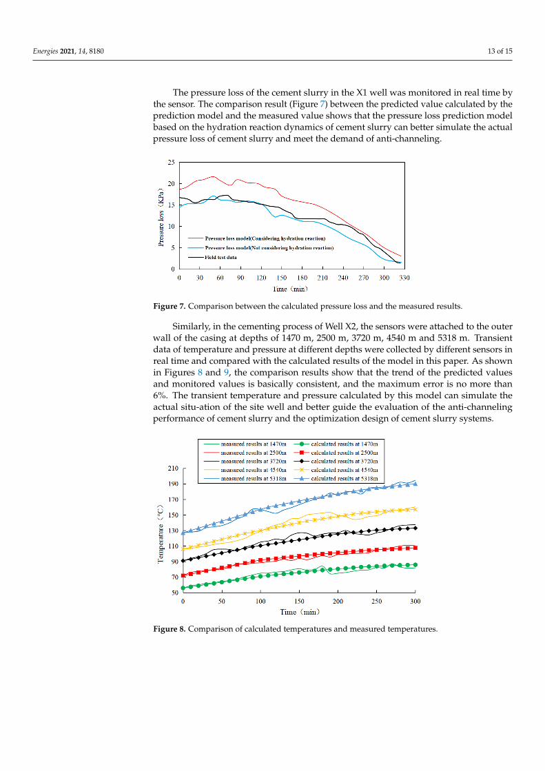
The pressure loss of the cement slurry in the X1 well was monitored in real time bythe sensor. The comparison result (Figure 7) between the predicted value calculated by theprediction model and the measured value shows that the pressure loss prediction modelbased on the hydration reaction dynamics of cement slurry can better simulate the actualpressure loss of cement slurry and meet the demand of anti-channeling.

Energies 2021, 14, x FOR PEER REVIEW 15 of 17

Figure 7. Comparison between the calculated pressure loss and the measured results.

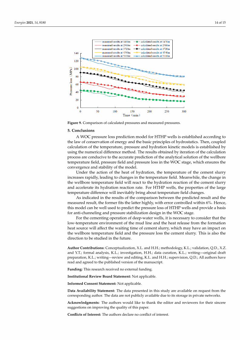
Similarly, in the cementing process of Well X2, the sensors were attached to the outer wall of the casing at depths of 1470 m, 2500 m, 3720 m, 4540 m and 5318 m. Transient data of temperature and pressure at different depths were collected by different sensors in real time and compared with the calculated results of the model in this paper. As shown in Figures 8 and 9, the comparison results show that the trend of the predicted values and monitored values is basically consistent, and the maximum error is no more than 6%. The transient temperature and pressure calculated by this model can simulate the actual situ-ation of the site well and better guide the evaluation of the anti-channeling performance of cement slurry and the optimization design of cement slurry systems.

Figure 8. Comparison of calculated temperatures and measured temperatures.

Figure 7. Comparison between the calculated pressure loss and the measured results.

Similarly, in the cementing process of Well X2, the sensors were attached to the outerwall of the casing at depths of 1470 m, 2500 m, 3720 m, 4540 m and 5318 m. Transientdata of temperature and pressure at different depths were collected by different sensors inreal time and compared with the calculated results of the model in this paper. As shownin Figures 8 and 9, the comparison results show that the trend of the predicted valuesand monitored values is basically consistent, and the maximum error is no more than6%. The transient temperature and pressure calculated by this model can simulate theactual situ-ation of the site well and better guide the evaluation of the anti-channelingperformance of cement slurry and the optimization design of cement slurry systems.

Energies 2021, 14, x FOR PEER REVIEW 15 of 17

Figure 7. Comparison between the calculated pressure loss and the measured results.

Similarly, in the cementing process of Well X2, the sensors were attached to the outer wall of the casing at depths of 1470 m, 2500 m, 3720 m, 4540 m and 5318 m. Transient data of temperature and pressure at different depths were collected by different sensors in real time and compared with the calculated results of the model in this paper. As shown in Figures 8 and 9, the comparison results show that the trend of the predicted values and monitored values is basically consistent, and the maximum error is no more than 6%. The transient temperature and pressure calculated by this model can simulate the actual situ-ation of the site well and better guide the evaluation of the anti-channeling performance of cement slurry and the optimization design of cement slurry systems.

Figure 8. Comparison of calculated temperatures and measured temperatures. Figure 8. Comparison of calculated temperatures and measured temperatures.

Energies 2021, 14, 8180 14 of 15Energies 2021, 14, x FOR PEER REVIEW 16 of 17

Figure 9. Comparison of calculated pressures and measured pressures.

5. Conclusions A WOC pressure loss prediction model for HTHP wells is established according to

the law of conservation of energy and the basic principles of hydrostatics. Then, coupled calculation of the temperature, pressure and hydration kinetic models is established by using the numerical difference method. The results obtained by iteration of the calculation process are conducive to the accurate prediction of the analytical solution of the wellbore temperature field, pressure field and pressure loss in the WOC stage, which ensures the convergence and stability of the model.

Under the action of the heat of hydration, the temperature of the cement slurry in-creases rapidly, leading to changes in the temperature field. Meanwhile, the change in the wellbore temperature field will react to the hydration reaction of the cement slurry and accelerate its hydration reaction rate. For HTHP wells, the properties of the large temper-ature difference will inevitably bring about temperature field changes.

As indicated in the results of the comparison between the predicted result and the measured result, the former fits the latter highly, with error controlled within 6%. Hence, this model can be well used to predict the pressure loss of HTHP wells and provide a basis for anti-channeling and pressure stabilization design in the WOC stage.

For the cementing operation of deep-water wells, it is necessary to consider that the low-temperature environment of the mud line and the heat release from the formation heat source will affect the waiting time of cement slurry, which may have an impact on the wellbore temperature field and the pressure loss the cement slurry. This is also the direction to be studied in the future.

Author Contributions: Conceptualization, X.L. and H.H.; methodology, K.L.; validation, Q.D., X.Z. and Y.T.; formal analysis, K.L.; investigation, H.H.; data curation, K.L.; writing—original draft prep-aration, K.L.; writing—review and editing, K.L. and H.H.; supervision, Q.D.; All authors have read and agreed to the published version of the manuscript.

Funding: This research received no external funding

Institutional Review Board Statement: Not applicable.

Informed Consent Statement: Not applicable.

Data Availability Statement: The data presented in this study are available on request from the corresponding author. The data are not publicly available due to its storage in private networks.

Acknowledgments: The authors would like to thank the editor and reviewers for their sincere sug-gestions on improving the quality of this paper.

Conflicts of Interest: The authors declare no conflicts of interest.

Figure 9. Comparison of calculated pressures and measured pressures.

5. Conclusions

A WOC pressure loss prediction model for HTHP wells is established according tothe law of conservation of energy and the basic principles of hydrostatics. Then, coupledcalculation of the temperature, pressure and hydration kinetic models is established byusing the numerical difference method. The results obtained by iteration of the calculationprocess are conducive to the accurate prediction of the analytical solution of the wellboretemperature field, pressure field and pressure loss in the WOC stage, which ensures theconvergence and stability of the model.

Under the action of the heat of hydration, the temperature of the cement slurryincreases rapidly, leading to changes in the temperature field. Meanwhile, the change inthe wellbore temperature field will react to the hydration reaction of the cement slurryand accelerate its hydration reaction rate. For HTHP wells, the properties of the largetemperature difference will inevitably bring about temperature field changes.

As indicated in the results of the comparison between the predicted result and themeasured result, the former fits the latter highly, with error controlled within 6%. Hence,this model can be well used to predict the pressure loss of HTHP wells and provide a basisfor anti-channeling and pressure stabilization design in the WOC stage.

For the cementing operation of deep-water wells, it is necessary to consider that thelow-temperature environment of the mud line and the heat release from the formationheat source will affect the waiting time of cement slurry, which may have an impact onthe wellbore temperature field and the pressure loss the cement slurry. This is also thedirection to be studied in the future.

Author Contributions: Conceptualization, X.L. and H.H.; methodology, K.L.; validation, Q.D., X.Z.and Y.T.; formal analysis, K.L.; investigation, H.H.; data curation, K.L.; writing—original draftpreparation, K.L.; writing—review and editing, K.L. and H.H.; supervision, Q.D.; All authors haveread and agreed to the published version of the manuscript.

Funding: This research received no external funding.

Institutional Review Board Statement: Not applicable.

Informed Consent Statement: Not applicable.

Data Availability Statement: The data presented in this study are available on request from thecorresponding author. The data are not publicly available due to its storage in private networks.

Acknowledgments: The authors would like to thank the editor and reviewers for their sinceresuggestions on improving the quality of this paper.

Conflicts of Interest: The authors declare no conflict of interest.

Energies 2021, 14, 8180 15 of 15

References1. Ravi, K.; Biezen, E.N.; Lightford, S.C.; Hibbert, A.; Greaves, C. Deepwater cementing challenges. Paper SPE56534. In Proceedings

of the SPE Annual Technical Conference and Exhibition, Houston, TX, USA, 26–29 September 1999.2. Chen, W. Status and challenges of Chinese deepwater oil and gas development. Petrol. Sci. 2011, 8, 477–484. [CrossRef]3. Christian, W.W.; Chatterji, J.; Ostroot, G.W. Gas leakage in primary cementing-a field study and laboratory investigation. J. Petrol.

Technol. 1976, 28, 1361–1369. [CrossRef]4. Wilkins, R.P.; Free, D. A new approach to the prediction of gas flow after cementing. In SPE/IADC Drilling Conference; Society of

Petroleum Engineers: New Orleans, LA, USA, 1989.5. Kremieniewski, M.; Wisniowski, R.; Stryczek, S.; Orłowicz, G. Possibilities of Limiting Migration of Natural Gas in Boreholes in

the Context of Laboratory Studies. Energies 2021, 14, 4251. [CrossRef]6. Tao, C.; Rosenbaum, E.; Kutchko, B.G.; Massoudi, M. A Brief Review of Gas Migration in Oilwell Cement Slurries. Energies 2021,

124, 2369. [CrossRef]7. API RP 10B-6. Recommended Practice on Determining the Static Gel Strength of Cement Formulations, 1st ed.; American Petroleum

Institute (API): Washington, DC, USA, 2014.8. Vazquez, G.; Blanco, A.M.; Colina, A.M. A Methodology to Evaluate the Gas Migration in Cement Slurries. In SPE Latin American

and Caribbean Petroleum Engineering Conference; Society of Petroleum Engineers: Rio de Janeiro, Brazil, 2005.9. Carter, G.; Slagle, K. A study of completion practices to minimize gas communication. J. Petrol. Technol. 1972, 24, 1170–1174.

[CrossRef]10. Sabins, F.L.; Tinsley, J.M.; Sutton, D.L. Transition time of cement slurries between the fluid and set states. SPE J. 1982, 22, 875–882.

[CrossRef]11. Sabins, F.L.; Sutton, D.L. The Relationship of Thickening Time, Gel Strength, and Compressive Strength of Oilwell Cements. SPE

Prod. Oper. 1986, 1, 143–152. [CrossRef]12. Drecq, P.; Parcevaux, P.A. A single technique solves gas migration problems across a wide range of conditions. In Proceedings of

the International Meeting on Petroleum Engineering, Tianjin, China, 1–4 November 1988.13. Sun, Z. The Relationship of Cement Slurry’s Three Pore Pressure Drops due to Settling, Settling-Gelling and Hydrated Volume

Shrinking-Gelling. China Offshore Oil Gas. 1999, 11, 51–54.14. Zhang, X.; Guo, X.; Yang, Y. A Laboratorial Research on Estimating Channeling-Preventing Ability of Cement Slurry by Use of

Gel Strength Method. Nat. Gas. Ind. 2001, 21, 52–55.15. Zhang, X.; Liu, C.; Yang, Y. The important influence of cement slurry’s stability on weight-loss. J. Southwest Pet. Inst. 2004, 26,

68–70.16. Lin, F.; Meyer, C. Hydration kinetics modeling of Portland cement considering the effects of curing temperature and applied

pressure. Cem. Concr. Res. 2009, 39, 255–265. [CrossRef]17. Bu, Y.; Mu, H.; Jiang, L.; Liu, W.; Wei, X.; Wen, S. Modeling and laboratory studies of cement slurry weight loss. Drill. Fluid

Complet.Fluid 2007, 24, 52–54.18. Zhou, S.; Li, G.; Chu, Y. Sectional design for anti-gas channeling cementing. Pet. Drill. Tech. 2013, 45, 52–55.19. Cheng, X.; Liu, K.; Li, Z.; Guo, X. Structure and properties of oil well cement slurry during liquid-solid transition. Acta Pet. Sinica

2016, 37, 1287–1292.20. Liu, Y.; Chen, M.; Shi, F.; Li, Y.; Xian, M. Study and application of a technology for evaluating pressure loss of cement plug. Drill.

Flu Complet. Fluid 2019, 37, 749–753.21. Zhu, H.; Qu, J.; Liu, A.; Zou, J.; Xu, J. A New Method to Evaluate the Gas Migration for Cement Slurries. Oilfield Chem. 2012, 29,

353–356.22. Li, Z.; Vandenbossche, J.M.; Iannacchione, A.T.; Brigham, J.C.; Kutchko, B.G. Theory-based review of limitations with static gel

strength in cement/matrix characterization. SPE Drill Complet. 2016, 31, 145–158. [CrossRef]23. Wooley, G.R. Computing downhole temperatures in circulation, injection, and production wells. J. Petrol. Technol. 1980, 32,

1509–1522. [CrossRef]24. Cooke, C.E.; Kluck, M.P.; Medrano, R. Field measurements of annular pressure and temperature during primary cementing. J.

Petrol. Technol. 1983, 35, 1429–1438. [CrossRef]25. Krstulovic, R.; Dabic, P. A conceptual model of the cement hydration process. Cem. Concr. Res. 2000, 30, 693–698. [CrossRef]26. Moore, P.L. Drilling Practice Manual; Petroleum Publishing, Co.: Tulsa, OK, USA, 1974.27. Wang, X.; Sun, B.; Liu, S.; Li, Z.; Liu, Z.; Wang, Z.; Li, H.; Gao, Y. A coupled model of temperature and pressure based on

hydration kinetics during well cementing in deep water. Petrol. Explor. Dev. 2020, 47, 867–876. [CrossRef]28. Pang, X.; Jimenez, W.C.; Iverson, B.J. Hydration kinetics modeling of the effect of curing temperature and pressure on the heat

evolution of oil well cement. Cem. Concr. Res. 2013, 54, 69–76. [CrossRef]29. Sun, B.; Wang, X.; Wang, Z.; Gao, Y. Transient temperature calculation method for deep-water cementing based on hydration

kinetics model. Appl. Therm. Eng. 2018, 129, 1426–1434. [CrossRef]30. Wang, X.; Wang, Z.; Deng, X.; Sun, B.; Zhao, Y.; Fu, W. Coupled thermal model of wellbore and permafrost in Arctic regions. Appl.

Therm. Eng. 2017, 123, 1291–1299. [CrossRef]