As

Ma

b

c

a

ARRAA

KSWHAE

1

ieattaptcma

0h

Fluid Phase Equilibria 355 (2013) 12– 25

Contents lists available at ScienceDirect

Fluid Phase Equilibria

j our na l ho me pa ge: www.elsev ier .com/ locate / f lu id

practical method for the estimation of oil and water mutualolubilities

arco A. Satyroa,∗, John M. Shawb, Harvey W. Yarrantonc

Virtual Materials Group, Inc., Calgary, Alberta, CanadaUniversity of Alberta, Edmonton, Alberta, CanadaUniversity of Calgary, Calgary, Alberta, Canada

r t i c l e i n f o

rticle history:eceived 16 April 2013eceived in revised form 20 June 2013ccepted 22 June 2013vailable online 2 July 2013

eywords:olubilityater

ydrocarbonctivity coefficient modelquation of state

a b s t r a c t

A simple model is proposed for the calculation of oil and water mutual solubilities as a function oftemperature using the hydrocarbon specific gravity and Watson-K factor as correlating parameters. Themodel parameters were determined using a single consistent set of high quality solubility data collectedat the water or hydrocarbon saturation pressures at temperatures from 273 K and 573 K but primarilyfrom 298 K to 398 K. The hydrocarbon in water solubilities ranged over 11 orders of magnitude while thewater in hydrocarbons solubilities ranged over 4 orders of magnitude. Hydrocarbon types ranged fromlow molecular weight paraffins such as n-pentane to heavy aromatics such as anthracene. The averageabsolute error in the estimated solubilities of water in hydrocarbons over 621 data points was 34% andapproached the suggested underlying uncertainty in the reference data (30%). The average absolute errorin the estimated solubilities of hydrocarbons in water over 964 data points was 88% and exceeded thesuggested underlying uncertainty in the reference data (30%).

The model can be extended to higher temperatures using a procedure based on activity coefficientsor equations of state and is easily adapted to work with ill-defined hydrocarbon mixtures. Predictionand correlation of solubilities of water in kerosene, heavy oils, and bitumen were made at tempera-

tures, pressures, and compositions far removed from the original data used for model construction. Thecorrelation failed near the critical temperature of water because under these conditions, the propertieshydrocarbon-rich phases in the mixtures on which the correlation is based (Type II and Type IIIa phasebehaviour according to the van Konynenburg and Scott naming scheme) and those of water + heavyhydrocarbons (Type IIIb phase behaviour) diverge. A separate NRTL based correlation is presented for themutual solubility of water + heavy oils at temperatures close to the critical temperature of water.

. Introduction

The estimation of mutual solubilities of water and oil is anmportant part of the development of reliable simulation mod-ls. The amount of water dissolved in hydrocarbons defines themount of water side draws from crude distillation towers whilehe amount of dissolved hydrocarbons in aqueous streams is impor-ant for the design of water treatment systems. Water can also ben attractive solvent for oil upgrading at high pressures and tem-eratures, and reasonable estimates for mutual solubilities underhese conditions are vital for the design of the reactor and asso-

iated water and hydrocarbon recovery systems. Thermodynamicodels used for the simulation of hydrocarbon processes can usu-

lly provide reliable estimates of water in hydrocarbon solubilities;

∗ Corresponding author. Tel.: +1 403 397 2031.E-mail address: marco.satyro@virtualmaterials.com (M.A. Satyro).

378-3812/$ – see front matter © 2013 Elsevier B.V. All rights reserved.ttp://dx.doi.org/10.1016/j.fluid.2013.06.049

© 2013 Elsevier B.V. All rights reserved.

however, estimates for the solubility of hydrocarbons in water areusually poor [1].

Several techniques for the estimation of water solubility areavailable, based on empirical equations such as the ones found inthe API handbook [2], Tsonopoulos [3,4], and de Hemptinne et al.[5]. In general, these techniques have some or all of the followinglimitations: available only for n-alkanes; require constants to bedetermined for individual compounds; limited to a single temper-ature, usually 25 ◦C; parameters dependent on molecular structureinformation [6]. On the other hand, simple cubic equations of statedo not suffer from these limitations and can be tuned to provide rea-sonable representations of water solubility in hydrocarbons usinginteraction parameters in the vicinity of 0.5 [5].

The estimation of solubilities of hydrocarbons in water is more

complicated and few models are capable of predicting the solubil-ity of hydrocarbons in water [5,7]. There are some models availablebased on limited carbon number ranges at 25 ◦C [5,8–18] withspecific constants determined based on chemical types or group

M.A. Satyro et al. / Fluid Phase Eq

Nomenclature

a parameter for Eq. (15)b parameter for Eqs. (6) or (7) and (14) or (16)c parameter for Eqs. (6) or (7) and (14) or (17)d parameter for Eqs. (6) or (7) and (14) or (18)e parameter for Eq. (19)f Pade approximant term, Eq. (4)g Pade approximant term, Eq. (5)h enthalpy of solutionnp number of data pointsOF objective function for data regressionp0, p1, p2 empirical constants in Eq. (2)R gas constantSG specific gravityT absolute temperatureT0 reference temperature, 298.15 KTb normal boiling point (K)x solute mole fractionWk Watson (UOP) K

Subscriptshc hydrocarbonI data point indexs solventw water

Superscriptscalc calculated valueIUPAC experimental or recommended solubility value

from IUPAC∝ value at infinite dilution

Greek symbols˛ parameter for Eq. (9)

parameter for Eq. (8)�Kw Watson K departure from paraffin reference, Eq. (8)�SG specific gravity departure from paraffin reference,

Eq. (9)� activity coefficient

ceueaccae

ibqmbuwa

h[d

� NRTL interaction parameter

ontributions [19–21]. Currently available models are not easilyxtended to oil and water mixtures where the oil is characterizedsing distillation curves. The pseudo-components do not providenough information for the definition of a chemical type since theyctually represent the mixture of several compounds of differenthemical nature that boil at similar temperatures. The same handi-ap applies to group contribution based methods. Finally, currentlyvailable methods do not provide much information for criticalvaluation of the quality of their predictions.

Simple cubic equations of state using classic quadratic mix-ng rules are not capable of predicting accurate mutual solubilitiesecause they use a symmetric interaction parameter. This inade-uacy has been long known [22] and special interaction parametersust be used for the correct representation of hydrocarbon solu-

ilities in the water-rich phase. These interaction parameters aresually much smaller than those required to model the solubility ofater in a hydrocarbon-rich phase and point to the need for more

dvanced asymmetric mixing rules [23,24].

The recent publication of carefully screened water +

ydrocarbon mutual solubility data by Maczynski and coworkers8–18] provides an extensive and consistent set of data for theevelopment of solubility models and provided much of the

uilibria 355 (2013) 12– 25 13

motivation for this study. The objective of this work is to developa fully predictive model for the estimation of oil and water mutualsolubilities applicable to petroleum and not just defined compo-nents. The model is to have a built-in temperature dependency andmust be easily integrated into a process simulation environmentwhere it can be used to provide information for the calculation ofmodel specific interaction parameters as are commonly used inactivity coefficient or equation of state methods.

2. Database

The construction of a consistent database for model develop-ment was greatly facilitated by the availability of an extensive,critically evaluated series of papers on hydrocarbons and water sol-ubility published by Maczynski and coworkers [8–18]. This datacompilation reviewed the previous extensive work done in theIUPAC Solubility Series, Volumes 37 and 38 [25,26] with correctionsand included new published work up to 2006. This recent workprovides solubility data as a function of temperature for paraffins,naphthenes, aromatics, and other hydrocarbons ranging from C5 toC36 hydrocarbons.

The available data points were individually examined and qual-ity identifiers were assigned to them. Reference data are providedbased on specially constructed correlation functions for specificchemical families [8]. Experimental data differing from the refer-ence data by less than 30% at similar temperatures from differentsources are classified as “recommended” while those that dif-fer from the recommended data by more than 30% are classifiedas “doubtful”. Their criteria, based on an analysis of cycloalkane,alkane, isoalkanes and alkenes (hydrocarbon in water) and alkanesand alkenes (water in hydrocarbons), were applied to solubilitiesof hydrocarbons in water as well as water in hydrocarbons. If val-ues from only a single laboratory are available, even if they agreewith the reference data, they are classified as “tentative”. If val-ues are available but are deemed suspicious by the investigators,they are classified as “rejected”. In this work only “recommended”or “tentative” data points were used in the development of themodel. The uncertainty of individual data points is not accessibleand consequently statistical weighting cannot be applied to deter-mine model parameters. Hydrocarbons lighter than C5 were notincluded. Tables 1 and 2 summarize all the data as well the tem-perature and composition ranges used in the construction of themodel.

3. Model development

The principle objective is to develop a practical model that canbe used to estimate mutual solubilities for hydrocarbon + watermixtures at temperatures found in common chemical processes.The method should be easily implemented as an estimation proce-dure for the determination of interaction parameters for rigorousthermodynamic models, based either on equations of state or activ-ity coefficients. Further, restrictions and limitations dictated bythe diversity of phase behaviours exhibited by water + hydrocarbonmixtures, data uncertainty (noted above), and hydrocarbon char-acterization must be recognized at the outset and are discussedbelow.

Hydrocarbon compounds typically approach their critical tem-peratures remote from, and at lower temperatures than, the criticaltemperature of water. For such cases the hydrocarbon-rich phaseis the more volatile phase and the phase diagrams are typically

Type IIIa [27] according to the naming scheme of van Konynenburgand Scott [28]. There are also cases, such as 1-methylnaphthalene,tetralin, naphthalene and biphenyl + water where the phase dia-grams are Type II as reviewed by [29]. However, for a small but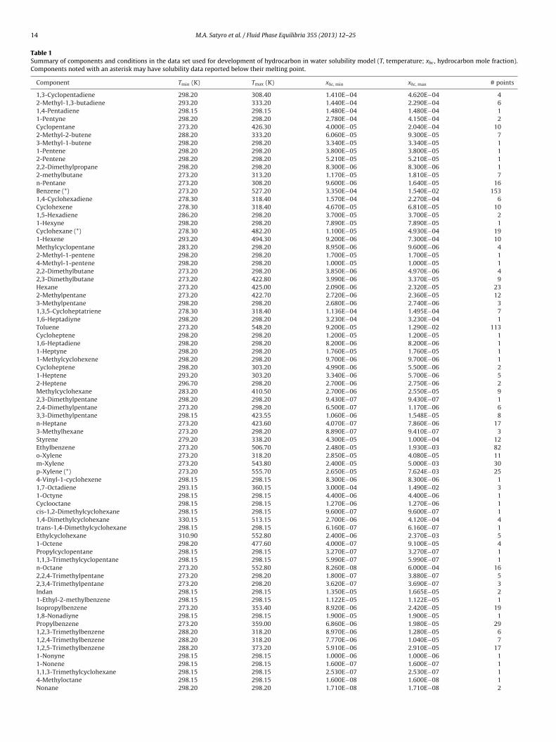

14 M.A. Satyro et al. / Fluid Phase Equilibria 355 (2013) 12– 25

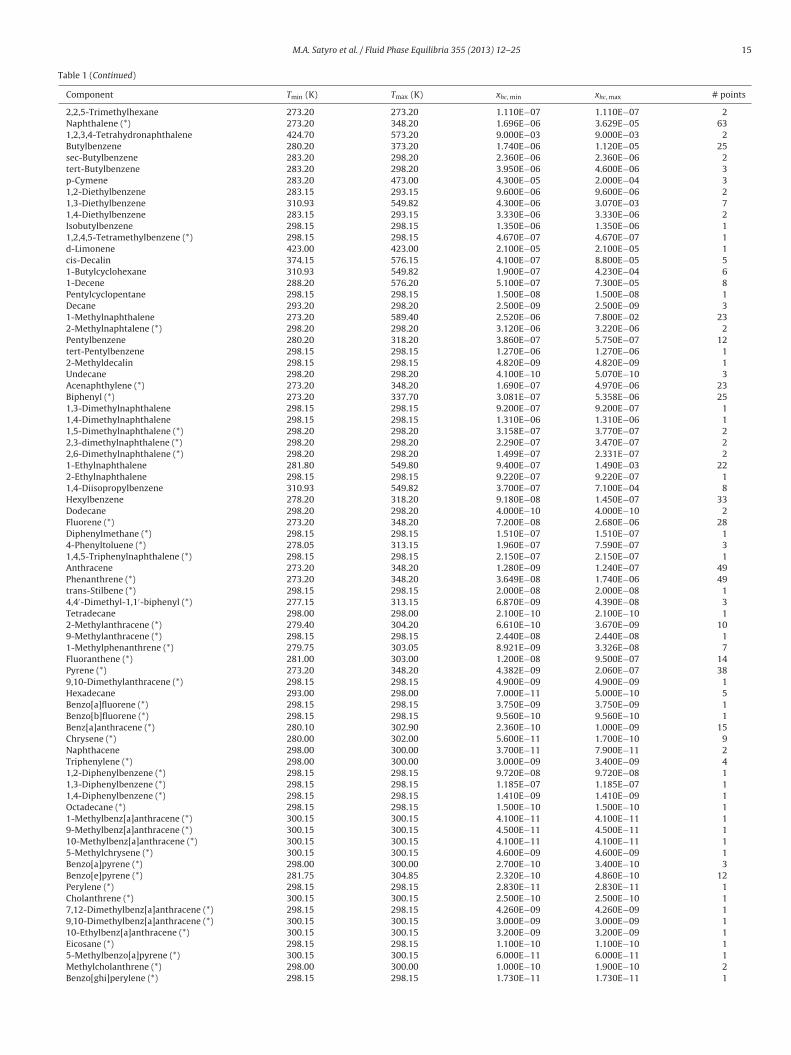
Table 1Summary of components and conditions in the data set used for development of hydrocarbon in water solubility model (T, temperature; xhc , hydrocarbon mole fraction).Components noted with an asterisk may have solubility data reported below their melting point.

Component Tmin (K) Tmax (K) xhc, min xhc, max # points

1,3-Cyclopentadiene 298.20 308.40 1.410E−04 4.620E−04 42-Methyl-1,3-butadiene 293.20 333.20 1.440E−04 2.290E−04 61,4-Pentadiene 298.15 298.15 1.480E−04 1.480E−04 11-Pentyne 298.20 298.20 2.780E−04 4.150E−04 2Cyclopentane 273.20 426.30 4.000E−05 2.040E−04 102-Methyl-2-butene 288.20 333.20 6.060E−05 9.300E−05 73-Methyl-1-butene 298.20 298.20 3.340E−05 3.340E−05 11-Pentene 298.20 298.20 3.800E−05 3.800E−05 12-Pentene 298.20 298.20 5.210E−05 5.210E−05 12,2-Dimethylpropane 298.20 298.20 8.300E−06 8.300E−06 12-methylbutane 273.20 313.20 1.170E−05 1.810E−05 7n-Pentane 273.20 308.20 9.600E−06 1.640E−05 16Benzene (*) 273.20 527.20 3.350E−04 1.540E−02 1531,4-Cyclohexadiene 278.30 318.40 1.570E−04 2.270E−04 6Cyclohexene 278.30 318.40 4.670E−05 6.810E−05 101,5-Hexadiene 286.20 298.20 3.700E−05 3.700E−05 21-Hexyne 298.20 298.20 7.890E−05 7.890E−05 1Cyclohexane (*) 278.30 482.20 1.100E−05 4.930E−04 191-Hexene 293.20 494.30 9.200E−06 7.300E−04 10Methylcyclopentane 283.20 298.20 8.950E−06 9.600E−06 42-Methyl-1-pentene 298.20 298.20 1.700E−05 1.700E−05 14-Methyl-1-pentene 298.20 298.20 1.000E−05 1.000E−05 12,2-Dimethylbutane 273.20 298.20 3.850E−06 4.970E−06 42,3-Dimethylbutane 273.20 422.80 3.990E−06 3.370E−05 9Hexane 273.20 425.00 2.090E−06 2.320E−05 232-Methylpentane 273.20 422.70 2.720E−06 2.360E−05 123-Methylpentane 298.20 298.20 2.680E−06 2.740E−06 31,3,5-Cycloheptatriene 278.30 318.40 1.136E−04 1.495E−04 71,6-Heptadiyne 298.20 298.20 3.230E−04 3.230E−04 1Toluene 273.20 548.20 9.200E−05 1.290E−02 113Cycloheptene 298.20 298.20 1.200E−05 1.200E−05 11,6-Heptadiene 298.20 298.20 8.200E−06 8.200E−06 11-Heptyne 298.20 298.20 1.760E−05 1.760E−05 11-Methylcyclohexene 298.20 298.20 9.700E−06 9.700E−06 1Cycloheptene 298.20 303.20 4.990E−06 5.500E−06 21-Heptene 293.20 303.20 3.340E−06 5.700E−06 52-Heptene 296.70 298.20 2.700E−06 2.750E−06 2Methylcyclohexane 283.20 410.50 2.700E−06 2.550E−05 92,3-Dimethylpentane 298.20 298.20 9.430E−07 9.430E−07 12,4-Dimethylpentane 273.20 298.20 6.500E−07 1.170E−06 63,3-Dimethylpentane 298.15 423.55 1.060E−06 1.548E−05 8n-Heptane 273.20 423.60 4.070E−07 7.860E−06 173-Methylhexane 273.20 298.20 8.890E−07 9.410E−07 3Styrene 279.20 338.20 4.300E−05 1.000E−04 12Ethylbenzene 273.20 506.70 2.480E−05 1.930E−03 82o-Xylene 273.20 318.20 2.850E−05 4.080E−05 11m-Xylene 273.20 543.80 2.400E−05 5.000E−03 30p-Xylene (*) 273.20 555.70 2.650E−05 7.624E−03 254-Vinyl-1-cyclohexene 298.15 298.15 8.300E−06 8.300E−06 11,7-Octadiene 293.15 360.15 3.000E−04 1.490E−02 31-Octyne 298.15 298.15 4.400E−06 4.400E−06 1Cyclooctane 298.15 298.15 1.270E−06 1.270E−06 1cis-1,2-Dimethylcyclohexane 298.15 298.15 9.600E−07 9.600E−07 11,4-Dimethylcyclohexane 330.15 513.15 2.700E−06 4.120E−04 4trans-1,4-Dimethylcyclohexane 298.15 298.15 6.160E−07 6.160E−07 1Ethylcyclohexane 310.90 552.80 2.400E−06 2.370E−03 51-Octene 298.20 477.60 4.000E−07 9.100E−05 4Propylcyclopentane 298.15 298.15 3.270E−07 3.270E−07 11,1,3-Trimethylcyclopentane 298.15 298.15 5.990E−07 5.990E−07 1n-Octane 273.20 552.80 8.260E−08 6.000E−04 162,2,4-Trimethylpentane 273.20 298.20 1.800E−07 3.880E−07 52,3,4-Trimethylpentane 273.20 298.20 3.620E−07 3.690E−07 3Indan 298.15 298.15 1.350E−05 1.665E−05 21-Ethyl-2-methylbenzene 298.15 298.15 1.122E−05 1.122E−05 1Isopropylbenzene 273.20 353.40 8.920E−06 2.420E−05 191,8-Nonadiyne 298.15 298.15 1.900E−05 1.900E−05 1Propylbenzene 273.20 359.00 6.860E−06 1.980E−05 291,2,3-Trimethylbenzene 288.20 318.20 8.970E−06 1.280E−05 61,2,4-Trimethylbenzene 288.20 318.20 7.770E−06 1.040E−05 71,2,5-Trimethylbenzene 288.20 373.20 5.910E−06 2.910E−05 171-Nonyne 298.15 298.15 1.000E−06 1.000E−06 11-Nonene 298.15 298.15 1.600E−07 1.600E−07 11,1,3-Trimethylcyclohexane 298.15 298.15 2.530E−07 2.530E−07 14-Methyloctane 298.15 298.15 1.600E−08 1.600E−08 1Nonane 298.20 298.20 1.710E−08 1.710E−08 2

M.A. Satyro et al. / Fluid Phase Equilibria 355 (2013) 12– 25 15

Table 1 (Continued)

Component Tmin (K) Tmax (K) xhc, min xhc, max # points

2,2,5-Trimethylhexane 273.20 273.20 1.110E−07 1.110E−07 2Naphthalene (*) 273.20 348.20 1.696E−06 3.629E−05 631,2,3,4-Tetrahydronaphthalene 424.70 573.20 9.000E−03 9.000E−03 2Butylbenzene 280.20 373.20 1.740E−06 1.120E−05 25sec-Butylbenzene 283.20 298.20 2.360E−06 2.360E−06 2tert-Butylbenzene 283.20 298.20 3.950E−06 4.600E−06 3p-Cymene 283.20 473.00 4.300E−05 2.000E−04 31,2-Diethylbenzene 283.15 293.15 9.600E−06 9.600E−06 21,3-Diethylbenzene 310.93 549.82 4.300E−06 3.070E−03 71,4-Diethylbenzene 283.15 293.15 3.330E−06 3.330E−06 2Isobutylbenzene 298.15 298.15 1.350E−06 1.350E−06 11,2,4,5-Tetramethylbenzene (*) 298.15 298.15 4.670E−07 4.670E−07 1d-Limonene 423.00 423.00 2.100E−05 2.100E−05 1cis-Decalin 374.15 576.15 4.100E−07 8.800E−05 51-Butylcyclohexane 310.93 549.82 1.900E−07 4.230E−04 61-Decene 288.20 576.20 5.100E−07 7.300E−05 8Pentylcyclopentane 298.15 298.15 1.500E−08 1.500E−08 1Decane 293.20 298.20 2.500E−09 2.500E−09 31-Methylnaphthalene 273.20 589.40 2.520E−06 7.800E−02 232-Methylnaphtalene (*) 298.20 298.20 3.120E−06 3.220E−06 2Pentylbenzene 280.20 318.20 3.860E−07 5.750E−07 12tert-Pentylbenzene 298.15 298.15 1.270E−06 1.270E−06 12-Methyldecalin 298.15 298.15 4.820E−09 4.820E−09 1Undecane 298.20 298.20 4.100E−10 5.070E−10 3Acenaphthylene (*) 273.20 348.20 1.690E−07 4.970E−06 23Biphenyl (*) 273.20 337.70 3.081E−07 5.358E−06 251,3-Dimethylnaphthalene 298.15 298.15 9.200E−07 9.200E−07 11,4-Dimethylnaphthalene 298.15 298.15 1.310E−06 1.310E−06 11,5-Dimethylnaphthalene (*) 298.20 298.20 3.158E−07 3.770E−07 22,3-dimethylnaphthalene (*) 298.20 298.20 2.290E−07 3.470E−07 22,6-Dimethylnaphthalene (*) 298.20 298.20 1.499E−07 2.331E−07 21-Ethylnaphthalene 281.80 549.80 9.400E−07 1.490E−03 222-Ethylnaphthalene 298.15 298.15 9.220E−07 9.220E−07 11,4-Diisopropylbenzene 310.93 549.82 3.700E−07 7.100E−04 8Hexylbenzene 278.20 318.20 9.180E−08 1.450E−07 33Dodecane 298.20 298.20 4.000E−10 4.000E−10 2Fluorene (*) 273.20 348.20 7.200E−08 2.680E−06 28Diphenylmethane (*) 298.15 298.15 1.510E−07 1.510E−07 14-Phenyltoluene (*) 278.05 313.15 1.960E−07 7.590E−07 31,4,5-Triphenylnaphthalene (*) 298.15 298.15 2.150E−07 2.150E−07 1Anthracene 273.20 348.20 1.280E−09 1.240E−07 49Phenanthrene (*) 273.20 348.20 3.649E−08 1.740E−06 49trans-Stilbene (*) 298.15 298.15 2.000E−08 2.000E−08 14,4′-Dimethyl-1,1′-biphenyl (*) 277.15 313.15 6.870E−09 4.390E−08 3Tetradecane 298.00 298.00 2.100E−10 2.100E−10 12-Methylanthracene (*) 279.40 304.20 6.610E−10 3.670E−09 109-Methylanthracene (*) 298.15 298.15 2.440E−08 2.440E−08 11-Methylphenanthrene (*) 279.75 303.05 8.921E−09 3.326E−08 7Fluoranthene (*) 281.00 303.00 1.200E−08 9.500E−07 14Pyrene (*) 273.20 348.20 4.382E−09 2.060E−07 389,10-Dimethylanthracene (*) 298.15 298.15 4.900E−09 4.900E−09 1Hexadecane 293.00 298.00 7.000E−11 5.000E−10 5Benzo[a]fluorene (*) 298.15 298.15 3.750E−09 3.750E−09 1Benzo[b]fluorene (*) 298.15 298.15 9.560E−10 9.560E−10 1Benz[a]anthracene (*) 280.10 302.90 2.360E−10 1.000E−09 15Chrysene (*) 280.00 302.00 5.600E−11 1.700E−10 9Naphthacene 298.00 300.00 3.700E−11 7.900E−11 2Triphenylene (*) 298.00 300.00 3.000E−09 3.400E−09 41,2-Diphenylbenzene (*) 298.15 298.15 9.720E−08 9.720E−08 11,3-Diphenylbenzene (*) 298.15 298.15 1.185E−07 1.185E−07 11,4-Diphenylbenzene (*) 298.15 298.15 1.410E−09 1.410E−09 1Octadecane (*) 298.15 298.15 1.500E−10 1.500E−10 11-Methylbenz[a]anthracene (*) 300.15 300.15 4.100E−11 4.100E−11 19-Methylbenz[a]anthracene (*) 300.15 300.15 4.500E−11 4.500E−11 110-Methylbenz[a]anthracene (*) 300.15 300.15 4.100E−11 4.100E−11 15-Methylchrysene (*) 300.15 300.15 4.600E−09 4.600E−09 1Benzo[a]pyrene (*) 298.00 300.00 2.700E−10 3.400E−10 3Benzo[e]pyrene (*) 281.75 304.85 2.320E−10 4.860E−10 12Perylene (*) 298.15 298.15 2.830E−11 2.830E−11 1Cholanthrene (*) 300.15 300.15 2.500E−10 2.500E−10 17,12-Dimethylbenz[a]anthracene (*) 298.15 298.15 4.260E−09 4.260E−09 19,10-Dimethylbenz[a]anthracene (*) 300.15 300.15 3.000E−09 3.000E−09 110-Ethylbenz[a]anthracene (*) 300.15 300.15 3.200E−09 3.200E−09 1Eicosane (*) 298.15 298.15 1.100E−10 1.100E−10 15-Methylbenzo[a]pyrene (*) 300.15 300.15 6.000E−11 6.000E−11 1Methylcholanthrene (*) 298.00 300.00 1.000E−10 1.900E−10 2Benzo[ghi]perylene (*) 298.15 298.15 1.730E−11 1.730E−11 1

16 M.A. Satyro et al. / Fluid Phase Equilibria 355 (2013) 12– 25

Table 1 (Continued)

Component Tmin (K) Tmax (K) xhc, min xhc, max # points

Dibenz[a,h]anthracene (*) 298.00 300.00 3.000E−11 3.900E−11 2Dibenz[a,j]anthracene (*) 300.15 300.15 7.800E−10 7.800E−10 1Picene (*) 300.15 300.15 1.600E−10 1.600E−10 110-Butylbenz[a]anthracene (*) 300.15 300.15 5.100E−10 5.100E−10 17-Pentylbenz[a]anthracene (*) 300.15 300.15 5.000E−11 5.000E−11 1

15

15

15

ice(cdthlwhwhaI

bnpridubtsim

twtawi

3

ae

woaibmtttn

Coronene (*) 298.15 298.Hexacosane (*) 298.15 298.Hexatriacontane (*) 298.15 298.

mportant subset of the experimental data, the hydrocarbon criti-al temperature is greater than that of water and these mixturesxhibit Type IIIb phase behaviour; for example, large n-alkanesC26 and above), indene, and heavy oils [29]. For these latterases, simple models spanning from ambient conditions to con-itions near the critical temperature of water are not valid becausehey only account for the interactions of sub- or near-criticalydrocarbon-rich liquid phases with a far from critical water-rich

iquid phase (Type II and Type IIIa behaviour). These interactionsith the water-rich liquid phase differ markedly from those of aydrocarbon-rich liquid phases remote from their critical pointsith a near critical water-rich liquid phase (Type IIIb). Hence, atigh temperatures, the properties of mixtures exhibiting Type IInd Type IIIa phase behaviour are expected to diverge from TypeIIb mixtures.

Heavy oils and bitumen are ill-defined and the uncertainty ofasic properties including their average molecular weight is sig-ificant. Molecular weights are typically measured with vapourressure osmometry or freezing point depression methods and areepeatable to only 15%. In addition, some asphaltenic componentsn the oil self-associate and the nature of the association and itsependence on temperature, pressure, and composition is not wellnderstood [30]. The solubility models reported in this work areased on mole fractions which are determined from mass frac-ions and average molecular weights for these fluids. Therefore,ystematic errors in molecular weights of ill-defined constituentsntroduce bias into the model vis-à-vis experimental solubility

easurements.With an initial focus on the Type II and Type IIIa data, a perturba-

ion approach and an infinite dilution activity coefficient approachere tested. Perturbation methods have been used successfully for

he modelling of hydrocarbon systems [31] while infinite dilutionctivity coefficients provide a simple, thermodynamically baseday to estimate solubilities. The development of each approach

s described below.

.1. Model 1: Perturbation method

This model for the solubility of both hydrocarbons in waternd water in hydrocarbons was based on the heat of solution asxpressed using standard thermodynamics:

∂ln x

∂(1/T)= −�h

R(1)

here x is mole fraction, T is absolute temperature, �h is the heatf solution, and R is the universal gas constant. Note, Eq. (1) is

simplification of the actual thermodynamic process of dissolv-ng materials in water since it neglects the formation of hydrogenonding and the resulting existence of a hydrocarbon solubilityinimum at around 298.15 K and 101.325 kPa. The shortcomings of

his equation can be alleviated by allowing the enthalpy of solutiono be a function of temperature as described below. It is also notedhat as temperatures and pressures increase the physico-chemicalature of water changes due to the reduction of its dielectric

8.560E−12 8.560E−12 18.000E−11 8.000E−11 16.100E−11 6.100E−11 1

constant, an effect not captured in the simple model proposed inthis work.

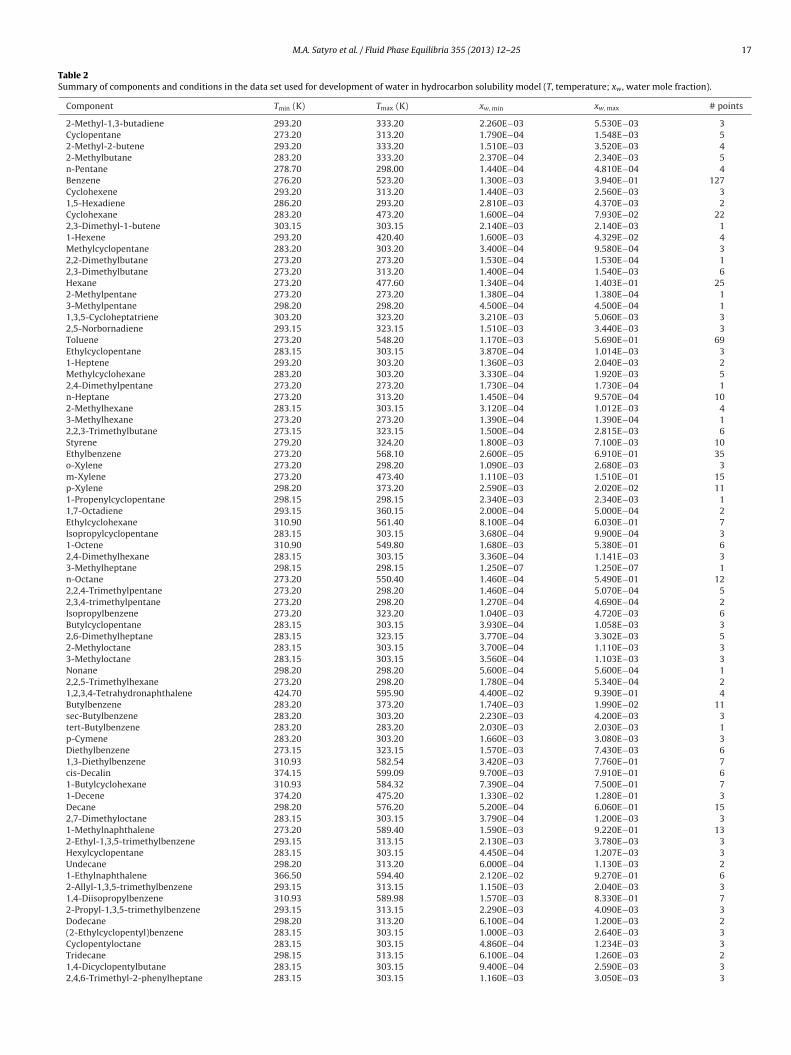
Eq. (1) can be expanded by allowing the enthalpy of solution tovary with temperature as:

ln x = p0 + p1

(1T

− 1T0

)+ p2

(T0

T+ ln

T

T0− 1)

(2)

where p0, p1, and p2 are empirical constants unique to eachhydrocarbon and phase. To make the model universal for allhydrocarbons, the empirical parameters in Eq. (2) are defined asperturbations around values determined based on paraffin dataonly as:

pi = p0i f 2

i g2i (3)

The perturbation functions f and g are defined based on differ-ences between the specific gravity and Watson-K factor betweenthe hydrocarbon of interest and an equivalent paraffin that boils atthe same temperature as the hydrocarbon of interest. The specificgravity SG is defined as the fluid density divided by the density ofliquid water at 60 F and 1 atm. The Watson-K factor is defined as thecubic root of the normal boiling point in R divided by the specificgravity. The specific gravity provides a coarse measure of molec-ular size while the Watson-K factor provides a coarse measure ofthe aromaticity of a hydrocarbon. They are also commonly avail-able properties coming from the oil characterization procedure andtherefore available when using the method to estimate solubilities.The perturbation functions take the form of Pade approximants assuggested by Twu [31] where he successfully used perturbationtheory to correlate critical temperatures, pressures, and volumesof many hydrocarbons:

fi = 1 + 2f 0i

1 − 2f 0i

(4)

gi = 1 + 2g0i

1 − 2g0i

(5)

f 0i = �SG

(bi√Tb

+(

ci + di√Tb

)�SG

)(6)

g0i = �Kw

(bi√Tb

+(

ci + di√Tb

)�Kw

)(7)

�SG = e˛(SG0−SG) − 1 (8)

�Kw = eˇ(Kw0−Kw) − 1 (9)

The model parameters for the water in hydrocarbon solubilitymodel are bi, ci, di, and ˇ, where i goes from 1 to 3 in accordancewith Eq. (2). The parameters are determined through non-linearregression using the objective function given by:

OFwater =np∑i=1

[ln

(xcalc

i,water

xIUPACi,water

)]2

(10)

M.A. Satyro et al. / Fluid Phase Equilibria 355 (2013) 12– 25 17

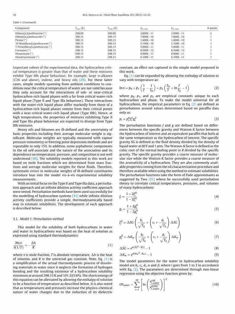
Table 2Summary of components and conditions in the data set used for development of water in hydrocarbon solubility model (T, temperature; xw , water mole fraction).

Component Tmin (K) Tmax (K) xw, min xw, max # points

2-Methyl-1,3-butadiene 293.20 333.20 2.260E−03 5.530E−03 3Cyclopentane 273.20 313.20 1.790E−04 1.548E−03 52-Methyl-2-butene 293.20 333.20 1.510E−03 3.520E−03 42-Methylbutane 283.20 333.20 2.370E−04 2.340E−03 5n-Pentane 278.70 298.00 1.440E−04 4.810E−04 4Benzene 276.20 523.20 1.300E−03 3.940E−01 127Cyclohexene 293.20 313.20 1.440E−03 2.560E−03 31,5-Hexadiene 286.20 293.20 2.810E−03 4.370E−03 2Cyclohexane 283.20 473.20 1.600E−04 7.930E−02 222,3-Dimethyl-1-butene 303.15 303.15 2.140E−03 2.140E−03 11-Hexene 293.20 420.40 1.600E−03 4.329E−02 4Methylcyclopentane 283.20 303.20 3.400E−04 9.580E−04 32,2-Dimethylbutane 273.20 273.20 1.530E−04 1.530E−04 12,3-Dimethylbutane 273.20 313.20 1.400E−04 1.540E−03 6Hexane 273.20 477.60 1.340E−04 1.403E−01 252-Methylpentane 273.20 273.20 1.380E−04 1.380E−04 13-Methylpentane 298.20 298.20 4.500E−04 4.500E−04 11,3,5-Cycloheptatriene 303.20 323.20 3.210E−03 5.060E−03 32,5-Norbornadiene 293.15 323.15 1.510E−03 3.440E−03 3Toluene 273.20 548.20 1.170E−03 5.690E−01 69Ethylcyclopentane 283.15 303.15 3.870E−04 1.014E−03 31-Heptene 293.20 303.20 1.360E−03 2.040E−03 2Methylcyclohexane 283.20 303.20 3.330E−04 1.920E−03 52,4-Dimethylpentane 273.20 273.20 1.730E−04 1.730E−04 1n-Heptane 273.20 313.20 1.450E−04 9.570E−04 102-Methylhexane 283.15 303.15 3.120E−04 1.012E−03 43-Methylhexane 273.20 273.20 1.390E−04 1.390E−04 12,2,3-Trimethylbutane 273.15 323.15 1.500E−04 2.815E−03 6Styrene 279.20 324.20 1.800E−03 7.100E−03 10Ethylbenzene 273.20 568.10 2.600E−05 6.910E−01 35o-Xylene 273.20 298.20 1.090E−03 2.680E−03 3m-Xylene 273.20 473.40 1.110E−03 1.510E−01 15p-Xylene 298.20 373.20 2.590E−03 2.020E−02 111-Propenylcyclopentane 298.15 298.15 2.340E−03 2.340E−03 11,7-Octadiene 293.15 360.15 2.000E−04 5.000E−04 2Ethylcyclohexane 310.90 561.40 8.100E−04 6.030E−01 7Isopropylcyclopentane 283.15 303.15 3.680E−04 9.900E−04 31-Octene 310.90 549.80 1.680E−03 5.380E−01 62,4-Dimethylhexane 283.15 303.15 3.360E−04 1.141E−03 33-Methylheptane 298.15 298.15 1.250E−07 1.250E−07 1n-Octane 273.20 550.40 1.460E−04 5.490E−01 122,2,4-Trimethylpentane 273.20 298.20 1.460E−04 5.070E−04 52,3,4-trimethylpentane 273.20 298.20 1.270E−04 4.690E−04 2Isopropylbenzene 273.20 323.20 1.040E−03 4.720E−03 6Butylcyclopentane 283.15 303.15 3.930E−04 1.058E−03 32,6-Dimethylheptane 283.15 323.15 3.770E−04 3.302E−03 52-Methyloctane 283.15 303.15 3.700E−04 1.110E−03 33-Methyloctane 283.15 303.15 3.560E−04 1.103E−03 3Nonane 298.20 298.20 5.600E−04 5.600E−04 12,2,5-Trimethylhexane 273.20 298.20 1.780E−04 5.340E−04 21,2,3,4-Tetrahydronaphthalene 424.70 595.90 4.400E−02 9.390E−01 4Butylbenzene 283.20 373.20 1.740E−03 1.990E−02 11sec-Butylbenzene 283.20 303.20 2.230E−03 4.200E−03 3tert-Butylbenzene 283.20 283.20 2.030E−03 2.030E−03 1p-Cymene 283.20 303.20 1.660E−03 3.080E−03 3Diethylbenzene 273.15 323.15 1.570E−03 7.430E−03 61,3-Diethylbenzene 310.93 582.54 3.420E−03 7.760E−01 7cis-Decalin 374.15 599.09 9.700E−03 7.910E−01 61-Butylcyclohexane 310.93 584.32 7.390E−04 7.500E−01 71-Decene 374.20 475.20 1.330E−02 1.280E−01 3Decane 298.20 576.20 5.200E−04 6.060E−01 152,7-Dimethyloctane 283.15 303.15 3.790E−04 1.200E−03 31-Methylnaphthalene 273.20 589.40 1.590E−03 9.220E−01 132-Ethyl-1,3,5-trimethylbenzene 293.15 313.15 2.130E−03 3.780E−03 3Hexylcyclopentane 283.15 303.15 4.450E−04 1.207E−03 3Undecane 298.20 313.20 6.000E−04 1.130E−03 21-Ethylnaphthalene 366.50 594.40 2.120E−02 9.270E−01 62-Allyl-1,3,5-trimethylbenzene 293.15 313.15 1.150E−03 2.040E−03 31,4-Diisopropylbenzene 310.93 589.98 1.570E−03 8.330E−01 72-Propyl-1,3,5-trimethylbenzene 293.15 313.15 2.290E−03 4.090E−03 3Dodecane 298.20 313.20 6.100E−04 1.200E−03 2(2-Ethylcyclopentyl)benzene 283.15 303.15 1.000E−03 2.640E−03 3Cyclopentyloctane 283.15 303.15 4.860E−04 1.234E−03 3Tridecane 298.15 313.15 6.100E−04 1.260E−03 21,4-Dicyclopentylbutane 283.15 303.15 9.400E−04 2.590E−03 32,4,6-Trimethyl-2-phenylheptane 283.15 303.15 1.160E−03 3.050E−03 3

18 M.A. Satyro et al. / Fluid Phase Equilibria 355 (2013) 12– 25

Table 2 (Continued)

Component Tmin (K) Tmax (K) xw, min xw, max # points

7,8-Dimethyltetradecane 293.15 323.15 9.670E−04 4.309E−03 4Hexadecane 293.00 323.00 8.670E−04 4.160E−03 4Coalinga 450.62 556.98 0.08927 0.5164 6Huntington Beach 413.31 560.33 0.1228 0.5026 7

0.1683 0.5108 60.2499 0.5913 70.5398 0.8455 8

Tmo

O

Tuo

3

ft

x

wwoEswtaccsl

l

wvss

c

�

Fb

TP(

Table 4NRTL model parameters for the estimation of hydrocarbon (i) solubility in water (s).

Parameter 1 2 3

A 0.4264 5.086 0.2732B 295.9 −187.4 −18.85

Peace River 450.62 555.98

Cat Canyon 432.45 561.34

Athabasca Bitumen 548.2 633.8

he model parameters for the hydrocarbon in water solubilityodel are a different set of bi, ci, di, and determined using the

bjective function given by:

Fhc =np∑i=1

[ln

(xcalc

i,hc

xIUPACi,hc

)]2

(11)

he optimized model parameters for Eqs. (8) and (9) for the sol-bility of hydrocarbon in water are summarized in Table 3. Theptimized exponents in Eqs. (8) and (9) are = 2.053 and = 4.531.

.2. Model 2: Infinite dilution activity coefficient approach

This model was developed based on the well-known fact thator sparingly soluble mixtures the solubility can be estimated ashe inverse of the infinite dilution activity coefficient, �∝:

i ≈ 1�∞

i

(12)

here i represents the solute, for example benzene in water orater in benzene and �∞

iis the infinite dilution activity coefficient

n i in solvent (water or hydrocarbon). An assumption implicit inq. (12) is that both water and hydrocarbons are liquids. Thus,olid hydrocarbons, designated with an asterisk (*) in Table 1,ere excluded from data regression and parameter evaluation for

he development of Model 2. The NRTL model [32] was selecteds the basic thermodynamic platform to determine the activityoefficients. NRTL is a well-known model capable of representingomplex phase equilibria, including water and hydrocarbon mutualolubilities. The activity coefficient at infinite dilution when calcu-ated using the NRTL model is given by:

n �∞i = �ise

−˛is�is + �si (13)

here �is is the interaction parameter between solute i and sol-ent s, �si is the interaction parameter between the solvent s andolute i, ˛is is the NRTL non-randomness parameter and subscript

represents the solvent, for example water or benzene.The interaction between solute and solvent requires an empiri-

al temperature dependency given by:

bis

is = ais +

T+ cis ln T (14)

inally the interaction energy between solvent and solute, �si, muste defined. It was found that a simple, temperature independent

able 3arameters for perturbation expansion specific gravity term (f) and Watson K termg).

Parameter B C D

f o0 10.13 1.461 −36.26

f o1 0.03103 0.9219 −0.02603

f o2 4.320 −3.254 −0.1027

go0 1.386 −0.01177 0.2144

go1 −0.4461 −0.003946 −0.008514

go2 −2.171 0.3755 −5.251

C 1.4561 −0.9645 −0.08160D 0.5850 −0.4342 −0.07145E 475.3 −277.0 −37.62

form was adequate for the correlation of both solubilities of hydro-carbons in water and solubilities of water in hydrocarbon. Theinteraction parameters are generalized as a function of specificgravity and Watson-K as follows.

ai,s = a1,s + a2,sSG + a3,sWK (15)

bi,s = b1,s + b2,sSG + b3,sWK (16)

ci,s = c1,s + c2,sSG + c3,sWK (17)

˛i,s = d1,s + d2,sSG + d3,sWK (18)

�s,i = e1,s + e2,sSG + e3,sWK (19)

The model was optimized using Eqs. (10) and (11) as described forModel 1. The optimized parameters for hydrocarbon in water andwater in hydrocarbon solubilities are summarized in Tables 4 and 5,respectively.

The NRTL interaction parameters used for the correlation of sol-ubility data (Eqs. (15)–(19)) are not directly applicable to a similarNRTL model used for phase equilibrium calculations since the �s,iterm is used as a correlating parameter in the development of thesolubility model. From a purely thermodynamic point of view itshould be calculated through the use of the corresponding interac-tion parameters that would model the solubility of solvent in solute.For example, the NRTL term �s,i (where i is for hydrocarbon and sis for water) was used as a correlating parameter without worry-ing about the actual accuracy of the estimated solubility of waterin hydrocarbon. Ideally one should regress mutual solubility datasimultaneously over a range of temperatures to develop an entirelyself-consistent model. Unfortunately the state of the experimentaldata does not allow for such a regression at this time. When usingthe proposed model for phase equilibrium calculations as com-

monly found in process simulation one should use the method tocalculate mutual solubility data at desired temperatures and thenregress these data to the desired thermodynamic model as will beshown later.

Table 5NRTL model parameters for the estimation of water solubility in hydrocarbons.

Parameter 1 2 3

A 80.55 10.05 −4.332B −1393 −2966 391.9C −6.912 −7.097 0.9115D −0.01890 −0.01282 0.001026E −57.47 74.82 −3.841

M.A. Satyro et al. / Fluid Phase Equilibria 355 (2013) 12– 25 19

1.E-12

1.E-09

1.E-06

1.E-03

1.E+00

1.E-12 1.E-061.E-09 1.E+001.E-03

Measured Solubility, Mole Fr.

Calc

ula

ted

So

lub

ilit

y, M

ole

Fr.

(a)

1.E-04

1.E-03

1.E-02

1.E-01

1.E+00

1.E+001.E-011.E-021.E-031.E-04

Measured Solubility, Mole Fr.

Calc

ula

ted

So

lub

ilit

y, M

ole

Fr.

(b)

wate

4

4

eiicithfT

udswiic

Fv

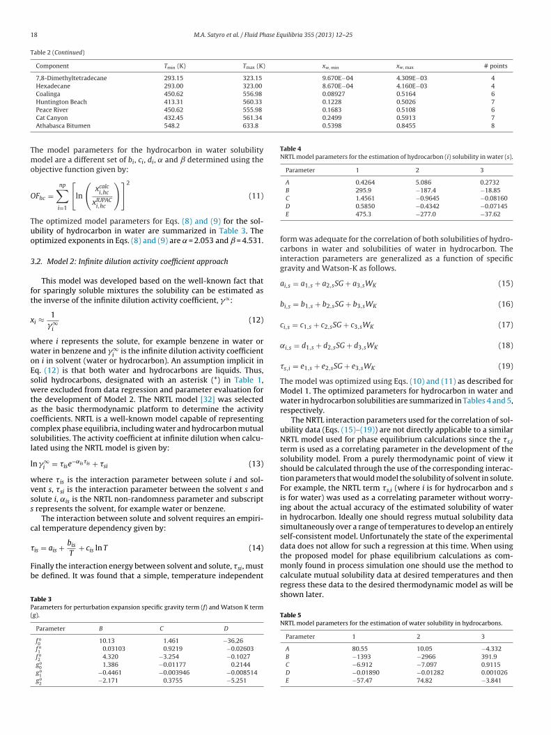
Fig. 1. Error dispersion plots for mutual solubilities of hydrocarbons and

. Results and discussion

.1. Model 1: Perturbation approach

At first glance, Table 6 and Fig. 1, the results for Model 1 werencouraging with an average absolute percent error equal to 122%,n the water-rich phase, and 45% in the hydrocarbon-rich phase. Anllustrative example, the predictions for the mutual solubilities ofyclohexane and water are shown in Fig. 2. To put these deviationsn perspective, consider that the data span 10 orders of magni-ude and include 160 different hydrocarbons for the modelling ofydrocarbon in water solubilities and 78 different hydrocarbons

or the modelling of water in hydrocarbon solubilities as shown inable 1.

Although reasonably good results were obtained, recent sim-lation data [33] suggests that there is a problem with n-paraffinata for carbons numbers above approximately 10. Simulation datauggests a smooth, regularly decreasing logarithm of solubilityith increasing carbon numbers but the data show a minimum

n solubility around carbon number equal to C16. There is signif-cant dispersion in the data, undoubtedly caused by the very lowoncentrations being measured and the associated experimental

1.E-06

1.E-05

1.E-04

1.E-03

1.E-02

1.E-01

1.E+00

200 300 400 500

Temperature, K

So

lute

Mo

le F

racti

on

in HC

in water

Model 1

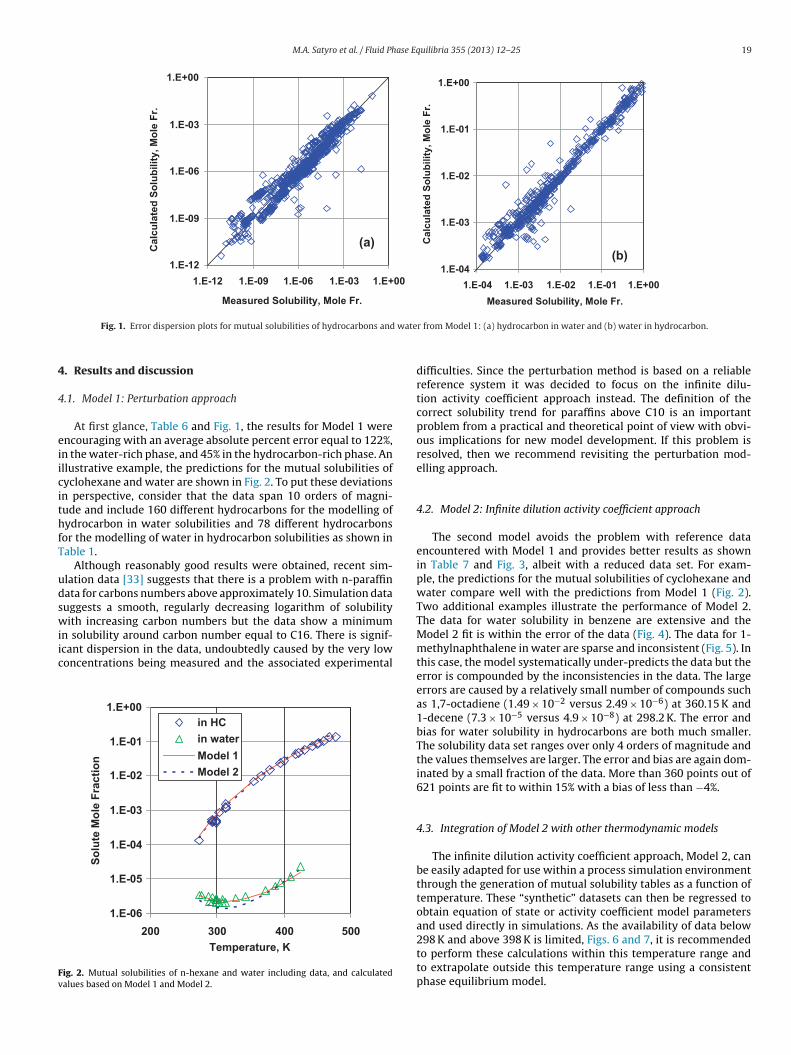
Model 2

ig. 2. Mutual solubilities of n-hexane and water including data, and calculatedalues based on Model 1 and Model 2.

r from Model 1: (a) hydrocarbon in water and (b) water in hydrocarbon.

difficulties. Since the perturbation method is based on a reliablereference system it was decided to focus on the infinite dilu-tion activity coefficient approach instead. The definition of thecorrect solubility trend for paraffins above C10 is an importantproblem from a practical and theoretical point of view with obvi-ous implications for new model development. If this problem isresolved, then we recommend revisiting the perturbation mod-elling approach.

4.2. Model 2: Infinite dilution activity coefficient approach

The second model avoids the problem with reference dataencountered with Model 1 and provides better results as shownin Table 7 and Fig. 3, albeit with a reduced data set. For exam-ple, the predictions for the mutual solubilities of cyclohexane andwater compare well with the predictions from Model 1 (Fig. 2).Two additional examples illustrate the performance of Model 2.The data for water solubility in benzene are extensive and theModel 2 fit is within the error of the data (Fig. 4). The data for 1-methylnaphthalene in water are sparse and inconsistent (Fig. 5). Inthis case, the model systematically under-predicts the data but theerror is compounded by the inconsistencies in the data. The largeerrors are caused by a relatively small number of compounds suchas 1,7-octadiene (1.49 × 10−2 versus 2.49 × 10−6) at 360.15 K and1-decene (7.3 × 10−5 versus 4.9 × 10−8) at 298.2 K. The error andbias for water solubility in hydrocarbons are both much smaller.The solubility data set ranges over only 4 orders of magnitude andthe values themselves are larger. The error and bias are again dom-inated by a small fraction of the data. More than 360 points out of621 points are fit to within 15% with a bias of less than −4%.

4.3. Integration of Model 2 with other thermodynamic models

The infinite dilution activity coefficient approach, Model 2, canbe easily adapted for use within a process simulation environmentthrough the generation of mutual solubility tables as a function oftemperature. These “synthetic” datasets can then be regressed to

obtain equation of state or activity coefficient model parametersand used directly in simulations. As the availability of data below298 K and above 398 K is limited, Figs. 6 and 7, it is recommendedto perform these calculations within this temperature range andto extrapolate outside this temperature range using a consistentphase equilibrium model.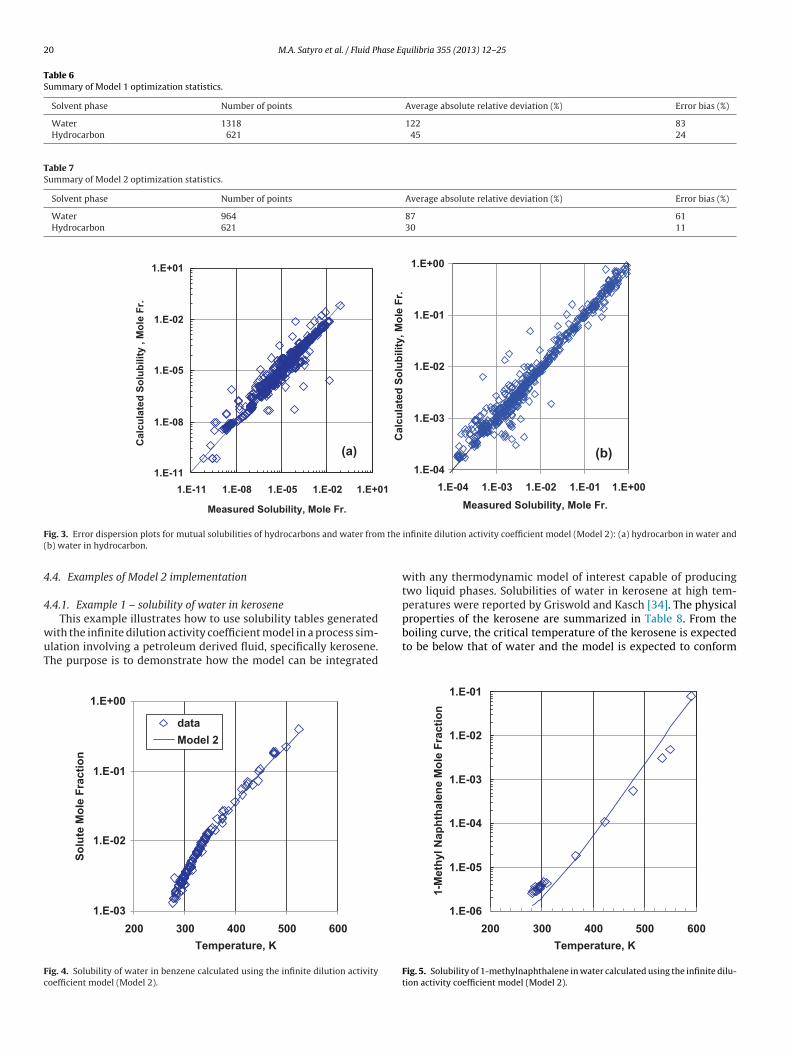

20 M.A. Satyro et al. / Fluid Phase Equilibria 355 (2013) 12– 25

Table 6Summary of Model 1 optimization statistics.

Solvent phase Number of points Average absolute relative deviation (%) Error bias (%)

Water 1318 122 83Hydrocarbon 621 45 24

Table 7Summary of Model 2 optimization statistics.

Solvent phase Number of points Average absolute relative deviation (%) Error bias (%)

Water 964 87 61Hydrocarbon 621 30 11

1.E-11

1.E-08

1.E-05

1.E-02

1.E+01

1.E-11 1.E-08 1.E-05 1.E-02 1.E+01

Measured Solubility, Mole Fr.

Calc

ula

ted

So

lub

ilit

y , M

ole

Fr.

(a)

1.E-04

1.E-03

1.E-02

1.E-01

1.E+00

1.E+001.E-011.E-021.E-031.E-04

Measured Solubility, Mole Fr.

Calc

ula

ted

So

lub

ilit

y, M

ole

Fr.

(b)

F the

(

4

4

wuT

Fc

ig. 3. Error dispersion plots for mutual solubilities of hydrocarbons and water fromb) water in hydrocarbon.

.4. Examples of Model 2 implementation

.4.1. Example 1 – solubility of water in kerosene

This example illustrates how to use solubility tables generated

ith the infinite dilution activity coefficient model in a process sim-lation involving a petroleum derived fluid, specifically kerosene.he purpose is to demonstrate how the model can be integrated

1.E-03

1.E-02

1.E-01

1.E+00

200 300 400 500 600

Temperature, K

So

lute

Mo

le F

rac

tio

n

data

Model 2

ig. 4. Solubility of water in benzene calculated using the infinite dilution activityoefficient model (Model 2).

infinite dilution activity coefficient model (Model 2): (a) hydrocarbon in water and

with any thermodynamic model of interest capable of producingtwo liquid phases. Solubilities of water in kerosene at high tem-peratures were reported by Griswold and Kasch [34]. The physical

properties of the kerosene are summarized in Table 8. From theboiling curve, the critical temperature of the kerosene is expectedto be below that of water and the model is expected to conform

1.E-06

1.E-05

1.E-04

1.E-03

1.E-02

1.E-01

200 300 400 500 600

Temperature, K

1-M

eth

yl N

ap

hth

ale

ne

Mo

le F

rac

tio

n

Fig. 5. Solubility of 1-methylnaphthalene in water calculated using the infinite dilu-tion activity coefficient model (Model 2).

M.A. Satyro et al. / Fluid Phase Equilibria 355 (2013) 12– 25 21

(A)

0

100

200

300

400

500

600

25

0

27

0

29

0

31

0

33

0

35

03

70

39

0

41

0

43

0

45

04

70

49

0

51

0

53

0

55

0

57

05

90

61

0

63

0

65

0

Temperature, K

Fre

qu

en

cy

(B)

0

0.05

0.1

0.15

0.2

0.25

0.3

0.35

0.4

350 400 450 500 550 600

Temperature, K

Waer

So

lub

ilit

y, M

ole

Fra

cti

on data

NRTL

(a)0

1

2

3

4

5

6

7

8

9

10

350 400 450 500 550 600

Temperature, K

Satu

rati

on

Pre

ssu

re, M

Pa

data

NRTL

(b)

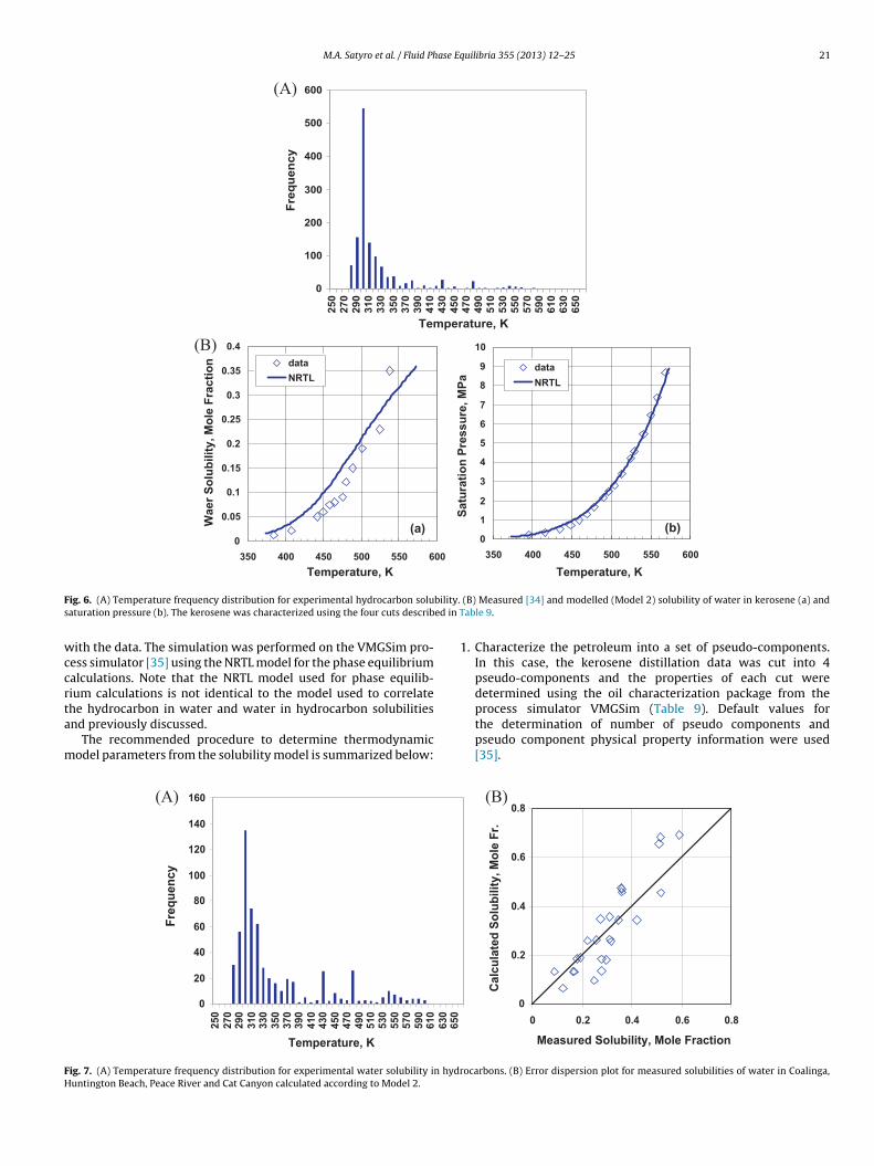
F bility.s ed in T

wccrta

m

FH

ig. 6. (A) Temperature frequency distribution for experimental hydrocarbon soluaturation pressure (b). The kerosene was characterized using the four cuts describ

ith the data. The simulation was performed on the VMGSim pro-ess simulator [35] using the NRTL model for the phase equilibriumalculations. Note that the NRTL model used for phase equilib-ium calculations is not identical to the model used to correlate

he hydrocarbon in water and water in hydrocarbon solubilitiesnd previously discussed.

The recommended procedure to determine thermodynamicodel parameters from the solubility model is summarized below:

(A)

0

20

40

60

80

100

120

140

160

25

0

27

02

90

31

03

30

35

03

70

39

0

41

04

30

45

04

70

49

05

10

53

05

50

57

05

90

61

0

63

06

50

Temperature, K

Fre

qu

en

cy

ig. 7. (A) Temperature frequency distribution for experimental water solubility in hydruntington Beach, Peace River and Cat Canyon calculated according to Model 2.

(B) Measured [34] and modelled (Model 2) solubility of water in kerosene (a) andable 9.

1. Characterize the petroleum into a set of pseudo-components.In this case, the kerosene distillation data was cut into 4pseudo-components and the properties of each cut weredetermined using the oil characterization package from the

process simulator VMGSim (Table 9). Default values forthe determination of number of pseudo components andpseudo component physical property information were used[35].

(B)

0

0.2

0.4

0.6

0.8

0 0.2 0.4 0.6 0.8

Measured Solubility, Mole Fraction

Calc

ula

ted

So

lub

ilit

y, M

ole

Fr.

ocarbons. (B) Error dispersion plot for measured solubilities of water in Coalinga,

22 M.A. Satyro et al. / Fluid Phase Equilibria 355 (2013) 12– 25

Table 8Physical properties of kerosene [34].

Property Value

API gravity 42Molecular weight (g/mol) 173Watson K 11.8IBP 475.93 K10% 487.04 K20% 491.48 K30% 494.26 K40% 497.59 K50% 500.93 K60% 503.15 K70% 505.93 K

2

3

4

Ncc

ftlfl

Table 11Heavy oil physical properties.

Oil Specific gravity Molecular weight (g/mol) Reference

Coalinga 1.00 439 [36]Huntington Beach 0.97 442 [36]Peace River 1.02 571 [36]

TK

TN

80% 509.82 K90% 515.37 KFBP 528.71 K

. Generate a table of mutual solubilities from 25 ◦C to 125 ◦C foreach oil cut with water using the infinite dilution activity coef-ficient model (four tables altogether). The temperature steps forsolubility calculations are arbitrary but we found out that 25 ◦Csteps were adequate in most situations.

. Regress the NRTL interaction parameters for each of the oilcut/water binaries using an objective function constructed basedon liquid–liquid equilibrium given by:

OF =npoints∑

i=1

nc∑j=1

(xhci �hc

i − xwi �w

i )2

(20)

It is recommended that the interaction parameters, �ij be madea function of temperature:

�ij = aij + bij

T+ cij ln T (21)

Note that any reasonable temperature dependency could be usedas commonly found in thermodynamic models supported bydifferent process simulators. In the case of NRTL one needs tochoose a value for the non-randomness parameter, or use it as afitting parameter. Here a fixed value, 0.2, was used.

. Install the NRTL interaction parameters in the simulator for flashcalculations.

ote, once the solubility tables are generated, the proposed pro-edure can be applied to any thermodynamic model, be it activityoefficient based or equation of state based.

The interaction parameters determined using this procedure

or kerosene and water are summarized in Table 10. With thehermodynamic model completed, it is straightforward to calcu-ate saturation conditions and mutual solubilities using standardow sheeting tools such as flashes and case studies. The estimated

able 9erosene pseudo-component properties.

Cut Mole fraction Standard density (kg/m3) Norm

1 0.1601 805.8 483.852 0.4773 812.9 497.153 0.2858 819.0 508.954 0.0768 826.9 523.15

able 10RTL interaction parameters calculated for kerosene cuts and water. Mutual solubility da

Cut ahc,w aw,hc

1 −6.945 6.105

2 −6.845 6.021

3 −6.754 5.951

4 −6.636 5.867

Cat Canyon 1.03 678 [36]Athabasca bitumen 1.02 550 [37]

water solubility and saturation pressures compare well with themeasured values, Fig. 6a and b respectively. The average absoluterelative deviation for the solubilities of water in kerosene is 46%(0.03 mole fraction). The average absolute deviation for the satura-tion pressures is 122 kPa.

4.4.2. Example 2 – solubility of water in heavy oilsIn this example, the applicability of the proposed method is

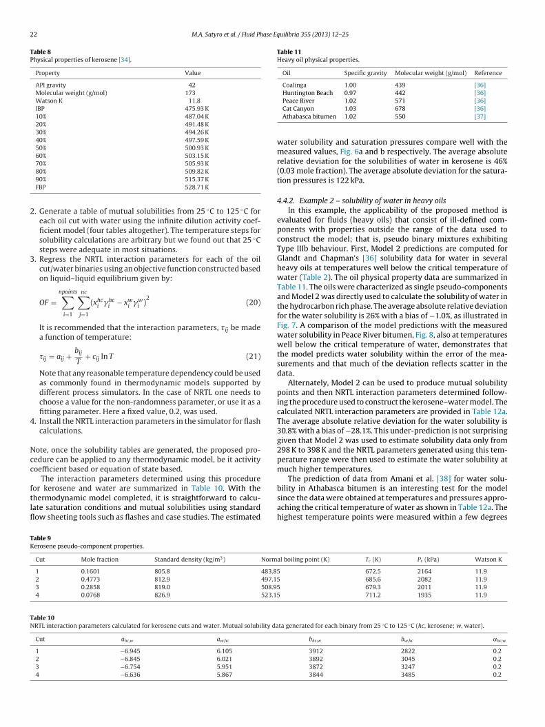
evaluated for fluids (heavy oils) that consist of ill-defined com-ponents with properties outside the range of the data used toconstruct the model; that is, pseudo binary mixtures exhibitingType IIIb behaviour. First, Model 2 predictions are computed forGlandt and Chapman’s [36] solubility data for water in severalheavy oils at temperatures well below the critical temperature ofwater (Table 2). The oil physical property data are summarized inTable 11. The oils were characterized as single pseudo-componentsand Model 2 was directly used to calculate the solubility of water inthe hydrocarbon rich phase. The average absolute relative deviationfor the water solubility is 26% with a bias of −1.0%, as illustrated inFig. 7. A comparison of the model predictions with the measuredwater solubility in Peace River bitumen, Fig. 8, also at temperatureswell below the critical temperature of water, demonstrates thatthe model predicts water solubility within the error of the mea-surements and that much of the deviation reflects scatter in thedata.

Alternately, Model 2 can be used to produce mutual solubilitypoints and then NRTL interaction parameters determined follow-ing the procedure used to construct the kerosene–water model. Thecalculated NRTL interaction parameters are provided in Table 12a.The average absolute relative deviation for the water solubility is30.8% with a bias of −28.1%. This under-prediction is not surprisinggiven that Model 2 was used to estimate solubility data only from298 K to 398 K and the NRTL parameters generated using this tem-perature range were then used to estimate the water solubility atmuch higher temperatures.

The prediction of data from Amani et al. [38] for water solu-

bility in Athabasca bitumen is an interesting test for the modelsince the data were obtained at temperatures and pressures appro-aching the critical temperature of water as shown in Table 12a. Thehighest temperature points were measured within a few degrees

al boiling point (K) Tc (K) Pc (kPa) Watson K

672.5 2164 11.9 685.6 2082 11.9 679.3 2011 11.9 711.2 1935 11.9

ta generated for each binary from 25 ◦C to 125 ◦C (hc, kerosene; w, water).

bhc,w bw,hc ˛hc,w

3912 2822 0.23892 3045 0.23872 3247 0.23844 3485 0.2

M.A. Satyro et al. / Fluid Phase Equilibria 355 (2013) 12– 25 23

Table 12aNRTL interaction parameters calculated for heavy oils and water based on synthetic mutual solubility data generated for each binary from 25 ◦C to 125 ◦C (hc, heavy oil; w,water).

Heavy oil ahc,w aw,hc bhc,w bw,hc ˛hc,w

Coalinga −4.388 4.656 3082 6963 0.2Huntington Beach −4.082 4.202 2932 6870 0.2Peace River −2.505 4.155 2418 8835 0.2Cat Canyon −2.548 3.976 2428 8100 0.2

Table 12bSolubility of water in the bitumen-rich liquid phase [38].

Temperature ± 0.3 (K) Pressure ± 0.07 (MPa) Measured water solubility ± 20% (wt.%) Modelled water solubility (wt%)

Model 2 Model 2 + APR High temperature Model 2

548.2 6.1 3.7 3.1 2.2 4.1573.1 9.0 5.3 5.3 3.1 6.0583.2 10.7 6.2 7.0 3.7 7.0593.1 12.7 7.7 9.6 4.3 8.2603.5 15.9 8.8 14.4 5.1 9.6

25.0 6.1 11.270.7 7.2 13.1Soluble 8.5 15.7

obtaoe(hiwdukmdTia

ePa

Fb

Table 13Water solubility estimates in Athabasca bitumen using Model 2.

Temperature (◦C) Mole fraction APR interaction parameter, kij

613.4 21.1 11.3

623.2 26.4 13.5

633.8 32.7 15.2

f the critical temperature of water. For this case, the distinctionetween Type II and Type IIIa phase behaviour in the data sets andhe Type IIIb behaviour of Athabasca bitumen + water is expected toffect the accuracy of calculated outcomes because the interactionf near critical water with a subcritical hydrocarbon (Type IIIb) isxpected to differ from subcritical water + subcritical hydrocarbonsType II, Type IIIa, Type IIIb), and subcritical water + near criticalydrocarbons (Type IIIa). From an experimental perspective, the

mpact of thermal decomposition on measured solubility values,hile compensated for in the measurement procedure, impactsata precision and accuracy. Random uncertainties of these sol-bility data, based on measurement repetition and validation withnown compounds up to 573 K, of ±20% are expected. Measure-ent bias, if present, underestimates solubility. Model 2, applied

irectly, treats the Athabasca bitumen + water pseudo binary as aype II binary mixture and significantly over-predicts the solubil-ty of water in Athabasca bitumen as the critical point of water ispproached (Table 12b).

An alternative approach is to use an equation of state toxtrapolate solubilities to higher temperatures. The Advancedeng–Robinson (APR) equation of state, a modification of the Pengnd Robinson equation of state [22] described elsewhere [35] was

0

0.1

0.2

0.3

0.4

0.5

0.6

0.7

400 450 500 550 600

Temperature, K

So

lute

Mo

le F

racti

on

data

simulation

ig. 8. Measured [36] and calculated (Model 2) solubility of water in Peace Riveritumen.

25 0.00242 0.3125 0.0481 0.25

used here. First solubilities were generated using Model 2 withinthe 298–398 K temperature range. Then, the APR was tuned to fitthese solubilities using a simple temperature dependency for thebinary interaction parameter, kij, between water and Athabascabitumen,

kij = 0.1009 + 59.35T

(22)

The fitted interaction parameters are listed in Table 13 and theestimated properties of Athabasca bitumen are shown in Table 14.

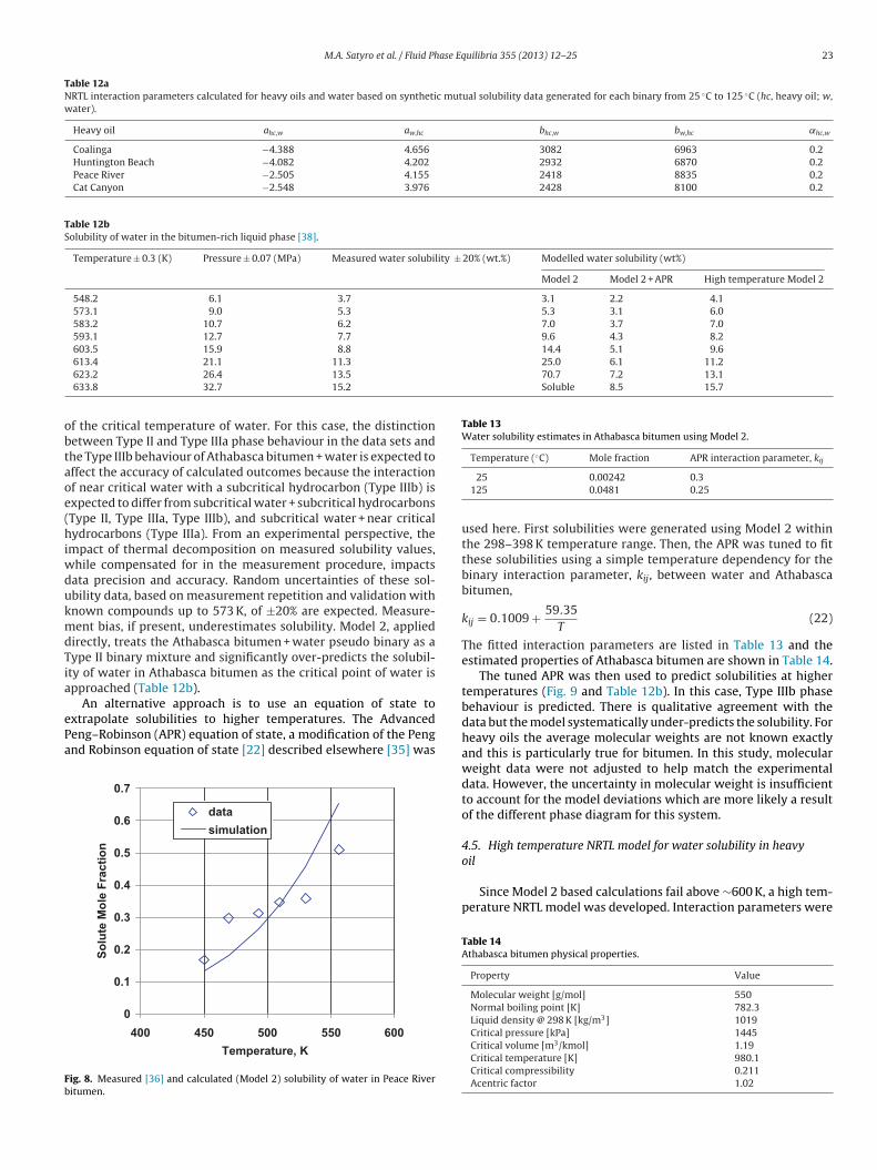
The tuned APR was then used to predict solubilities at highertemperatures (Fig. 9 and Table 12b). In this case, Type IIIb phasebehaviour is predicted. There is qualitative agreement with thedata but the model systematically under-predicts the solubility. Forheavy oils the average molecular weights are not known exactlyand this is particularly true for bitumen. In this study, molecularweight data were not adjusted to help match the experimentaldata. However, the uncertainty in molecular weight is insufficientto account for the model deviations which are more likely a resultof the different phase diagram for this system.

4.5. High temperature NRTL model for water solubility in heavy

oil

Since Model 2 based calculations fail above ∼600 K, a high tem-perature NRTL model was developed. Interaction parameters were

Table 14Athabasca bitumen physical properties.

Property Value

Molecular weight [g/mol] 550Normal boiling point [K] 782.3Liquid density @ 298 K [kg/m3] 1019Critical pressure [kPa] 1445Critical volume [m3/kmol] 1.19Critical temperature [K] 980.1Critical compressibility 0.211Acentric factor 1.02

24 M.A. Satyro et al. / Fluid Phase Equilibria 355 (2013) 12– 25

0

2

4

6

8

10

12

14

16

540 560 580 600 620 640

Temperature, K

Wate

r S

olu

bilit

y, w

t%

data

Model 2 + APR

Fig. 9. Measured [38] and predicted (Model 2 and APR) water solubility in Athabascabitumen.

Table 15High temperature NRTL model parameters for the estimation of water solubility inheavy oils.

Parameter 1 2 3

a −9.776 −12.34 −18.53b 0.000 0.000 0.000c 14.25 −9.437 3.027

ooTaiapFp

FN

0.0

0.1

0.2

0.3

0.4

0.5

0.6

0.7

0.8

0.9

1.0

0.0 0.2 0.4 0.6 0.8 1.0

Measured Solubility, Mole Fr.

Calc

ula

ted

So

lub

ilit

y, M

ole

Fr.

Huntington Beach

Coalinga

Cat Canyon

Peace River

Athabasca

d 0.5896 0.8993 −0.1144e 0.4410 −10.58 −3.004

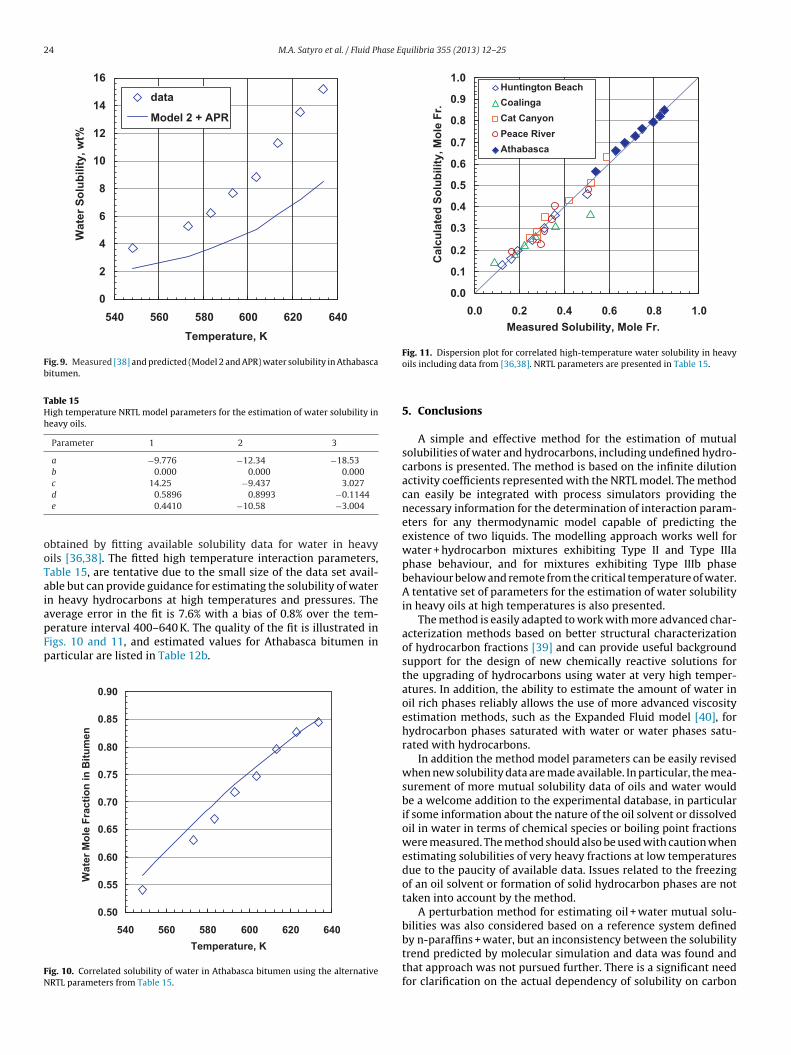
btained by fitting available solubility data for water in heavyils [36,38]. The fitted high temperature interaction parameters,able 15, are tentative due to the small size of the data set avail-ble but can provide guidance for estimating the solubility of watern heavy hydrocarbons at high temperatures and pressures. Theverage error in the fit is 7.6% with a bias of 0.8% over the tem-

erature interval 400–640 K. The quality of the fit is illustrated inigs. 10 and 11, and estimated values for Athabasca bitumen inarticular are listed in Table 12b.

0.50

0.55

0.60

0.65

0.70

0.75

0.80

0.85

0.90

540 560 580 600 620 640

Temperature, K

Wate

r M

ole

Fra

cti

on

in

Bit

um

en

ig. 10. Correlated solubility of water in Athabasca bitumen using the alternativeRTL parameters from Table 15.

Fig. 11. Dispersion plot for correlated high-temperature water solubility in heavyoils including data from [36,38]. NRTL parameters are presented in Table 15.

5. Conclusions

A simple and effective method for the estimation of mutualsolubilities of water and hydrocarbons, including undefined hydro-carbons is presented. The method is based on the infinite dilutionactivity coefficients represented with the NRTL model. The methodcan easily be integrated with process simulators providing thenecessary information for the determination of interaction param-eters for any thermodynamic model capable of predicting theexistence of two liquids. The modelling approach works well forwater + hydrocarbon mixtures exhibiting Type II and Type IIIaphase behaviour, and for mixtures exhibiting Type IIIb phasebehaviour below and remote from the critical temperature of water.A tentative set of parameters for the estimation of water solubilityin heavy oils at high temperatures is also presented.

The method is easily adapted to work with more advanced char-acterization methods based on better structural characterizationof hydrocarbon fractions [39] and can provide useful backgroundsupport for the design of new chemically reactive solutions forthe upgrading of hydrocarbons using water at very high temper-atures. In addition, the ability to estimate the amount of water inoil rich phases reliably allows the use of more advanced viscosityestimation methods, such as the Expanded Fluid model [40], forhydrocarbon phases saturated with water or water phases satu-rated with hydrocarbons.

In addition the method model parameters can be easily revisedwhen new solubility data are made available. In particular, the mea-surement of more mutual solubility data of oils and water wouldbe a welcome addition to the experimental database, in particularif some information about the nature of the oil solvent or dissolvedoil in water in terms of chemical species or boiling point fractionswere measured. The method should also be used with caution whenestimating solubilities of very heavy fractions at low temperaturesdue to the paucity of available data. Issues related to the freezingof an oil solvent or formation of solid hydrocarbon phases are nottaken into account by the method.

A perturbation method for estimating oil + water mutual solu-bilities was also considered based on a reference system definedby n-paraffins + water, but an inconsistency between the solubility

trend predicted by molecular simulation and data was found andthat approach was not pursued further. There is a significant needfor clarification on the actual dependency of solubility on carbon

ase Eq

nr

A

pJAePIa(RPdSE

R

[

[

[

[

[

[

[

[

[

[[

[

[[[[

[

[

[[[

[[[

[[[[

[[39] H. Loria, G. Hay, M.A. Satyro, Thermodynamic Modeling and Pro-

M.A. Satyro et al. / Fluid Ph

umber above decane, which offers a significant opportunity foresearch.

cknowledgements

The authors are grateful to Virtual Materials Group, Inc. forermission to publish this paper. The assistance of Mohammad

. Amani (University of Alberta), J. van Dorp (Shell Canada) and. Panagiotopoulos (Princeton University) is gratefully acknowl-dged. Initial motivation for this work came from discussions with. House, J. van Dorp (Shell Canada), G. Hay (VMG Canada), H.ketani (VMG Japan) and G. Jacobs (VMG USA). Harvey Yarrantonnd John M. Shaw also acknowledge the sponsors of the NSERCNatural Sciences and Engineering Research Council) Industrialesearch Chairs in Heavy Oil Properties and Processes (NSERC,etrobras, Schlumberger, and Shell), and in Petroleum Thermo-ynamics (NSERC, Alberta Innovates Energy and Environmentolutions, British Petroleum, ConocoPhillips, Nexen, Shell, Total&P Canada) respectively.

eferences

[1] M.A. Satyro, The role of thermodynamic modeling consistency in process sim-ulation, in: 8th World Congress of Chemical Engineering, Palais des Congres,Montreal, August 23–27, 2009.

[2] API Technical Data Book: Petroleum Refining, 5th ed., American PetroleumInstitute, 1992.

[3] C. Tsonopoulos, Fluid Phase Equilib. 156 (1999) 21–33.[4] C. Tsonopoulos, Fluid Phase Equilib. 196 (2001) 185–206.[5] J.-C. de Hemptinne, J.-M. Ledanois, P. Mougin, A. Barreau, Select Thermody-

namic Models for Process Simulation – A Practical Guide using a Three StepsMethodology, Editions Technip, France, 2012.

[6] C.J. Brady, J.R. Cunningham, G.M. Wilson, Water–hydrocarbonliquid–liquid–vapor equilibrium measurements to 530 F; GPA ResearchReport 62, 1982.

[7] J. Vidal, Thermodynamics – Applications in Chemical Engineering and thePetroleum Industry, Editions Technip, Paris, 2003.

[8] A. Maczynski, D. Shaw, M. Goral, B. Wisniewska-Goclowska, A. Skrzecz, Z.Maczynska, I. Owczarek, K. Blazej, M.-C. Haulait-Pirson, F. Kapuku, G.T. Hefter,A. Szafranski, J. Phys. Chem. Ref. Data 34 (2) (2005) 1399–1487.

[9] A. Maczynski, D. Shaw, M. Goral, B. Wisniewska-Goclowska, A. Skrzecz,I. Owczarek, K. Blazej, M.-C. Haulait-Pirson, G.T. Hefter, Z. Maczynska, A.Szafranski, C. Tsonopoulos, C.L. Young, J. Phys. Chem. Ref. Data 34 (2) (2005)477–542.

10] A. Maczynski, D. Shaw, M. Goral, B. Wisniewska-Goclowska, A. Skrzecz, I.

Owczarek, K. Blazej, M.-C. Haulait-Pirson, G.T. Hefter, Z. Maczynska, A. Szafran-ski, C.L. Young, J. Phys. Chem. Ref. Data 34 (2) (2005) 657–708.

11] A. Maczynski, D. Shaw, M. Goral, B. Wisniewska-Goclowska, A. Skrzecz, I.Owczarek, K. Blazej, M.-C. Haulait-Pirson, G.T. Hefter, F. Kapuku, Z. Maczynska,C.L. Young, J. Phys. Chem. Ref. Data 34 (2) (2005) 709–713.

[

uilibria 355 (2013) 12– 25 25

12] A. Maczynski, D. Shaw, M. Goral, B. Wisniewska-Goclowska, A. Skrzecz, I.Owczarek, K. Blazej, M.-C. Haulait-Pirson, G.T. Hefter, F. Kapuku, Z. Maczynska,C.L. Young, J. Phys. Chem. Ref. Data 34 (3) (2005) 1399–1487.

13] D.G. Shaw, A. Maczynski, D. Shaw, M. Goral, B. Wisniewska-Goclowska, A.Skrzecz, I. Owczarek, K. Blazej, M.-C. Haulait-Pirson, G.T. Hefter, Z. Maczynska,A. Szafranski, J. Phys. Chem. Ref. Data 34 (3) (2005) 1489–1553.

14] D.G. Shaw, A. Maczynski, D. Shaw, M. Goral, B. Wisniewska-Goclowska, A.Skrzecz, I. Owczarek, K. Blazej, M.-C. Haulait-Pirson, G.T. Hefter, F. Kapuku, Z.Maczynska, A. Szafranski, J. Phys. Chem. Ref. Data 34 (4) (2005) 2261–2298.

15] D.G. Shaw, A. Maczynski, D. Shaw, M. Goral, B. Wisniewska-Goclowska, A.Skrzecz, I. Owczarek, K. Blazej, M.-C. Haulait-Pirson, G.T. Hefter, F. Kapuku, Z.Maczynska, A. Szafranski, J. Phys. Chem. Ref. Data 34 (4) (2005) 2299–2345.

16] D.G. Shaw, A. Maczynski, D. Shaw, M. Goral, B. Wisniewska-Goclowska, A.Skrzecz, I. Owczarek, K. Blazej, M.-C. Haulait-Pirson, G.T. Hefter, P.L. Huyskens,F. Kapuku, Z. Maczynska, A. Szafranski, J. Phys. Chem. Ref. Data 35 (1) (2006)93–151.

17] D.G. Shaw, A. Maczynski, D. Shaw, M. Goral, B. Wisniewska-Goclowska, A.Skrzecz, I. Owczarek, K. Blazej, M.-C. Haulait-Pirson, G.T. Hefter, F. Kapuku, Z.Maczynska, A. Szafranski, J. Phys. Chem. Ref. Data 35 (1) (2006) 153–203.

18] D.G. Shaw, A. Maczynski, D. Shaw, M. Goral, B. Wisniewska-Goclowska, A.Skrzecz, I. Owczarek, K. Blazej, M.-C. Haulait-Pirson, G.T. Hefter, F. Kapuku, Z.Maczynska, A. Szafranski, J. Phys. Chem. Ref. Data 35 (2) (2006) 687–784.

19] A.V. Plyasunov, E.L. Shock, J. Chem. Eng. Data 46 (5) (2001) 1016–1019.20] N.V. Plyasunova, A.V. Plyasunov, E.L. Shock, J. Chem. Eng. Data 50 (1) (2005)

246–253.21] A.V. Plyasunov, N.V. Plyasunova, E.L. Shock, J. Chem. Eng. Data 51 (1) (2006)

1481–1490.22] D.-Y. Peng, D.B. Robinson, Can. J. Chem. Eng. 54 (1976) 595–599.23] I. Soreide, C. Whitson, Fluid Phase Equilib. 77 (1992) 217–240.24] V.N. Kabadi, R.P. Danner, Ind. Eng. Chem. Proc. Des. Dev. 24 (3) (1985) 537–541.25] D. Shaw (Ed.), IUPAC Solubility Data Series, vol. 37, Hydrocarbons with Water

and Seawater, Part I Hydrocarbons C5 to C7, Pergamon Press, New York, 1989.26] D. Shaw (Ed.), IUPAC Solubility Data Series, vol. 38, Hydrocarbons with Water

and Seawater, Part II: Hydrocarbons C8 to C36, Pergamon Press, New York,1989.

27] U.K. Deiters, T. Kraska, High Pressure Fluid Phase Equilibria – Phenomenologyand Computation, Elsevier, Amsterdam, 2012.

28] P.H. van Konynenburg, R.L. Scott, Phil. Trans. R. Soc. Lond. A 298 (1980) 495–540.29] M.J. Amani, M.R. Gray, J.M. Shaw, J. Supercrit. Fluids 77 (2013) 142–152.30] H.W. Yarranton, Asphaltene self-association, J. Dispers. Sci. Technol. 26 (1)

(2005) 5–8.31] H. Twu, Fluid Phase Equilib. 16 (1984) 137–150.32] H. Renon, J.M. Prausnitz, AIChE J. 14 (1968) 135–144.33] A.L. Ferguson, P.G. Debenedetti, A.Z. Panagiotopoulos, J. Phys. Chem. B 113

(2009) 6405–6414.34] J. Griswold, J.E. Kasch, Ind. Eng. Chem. 34 (7) (1942) 804–806.35] VMGSim User’s Manual version 7.0, Virtual Materials Group, Inc., 2012.36] C.A. Glandt, W.G. Chapman, SPE Res. Eng. 10 (1995) 59–64.37] A. BadamchiZadeh, H.W. Yarranton, W.Y. Svrcek, B.B. Maini, J. Can. Pet. Technol.

48 (1) (2009) 54–61.38] M.J. Amani, M.R. Gray, J.M. Shaw, Fluid Phase Equilibria (2013) (in press).

cess Simulation through PIONA Characterization, Energy Fuels (2013),http://dx.doi.org/10.1021/ef400286, Article ASAP.

40] H.W. Yarranton, M.A. Satyro, Expanded fluid based viscosity correlation forhydrocarbons, Ind. Eng. Chem. Res. 48 (7) (2009) 3640–3648.