O

Ao

JCa

b

c

d

a

A

R

R

9

A

K

L

S

D

A

O

d

0d

c o m p u t e r s a n d e l e c t r o n i c s i n a g r i c u l t u r e 6 4 ( 2 0 0 8 ) 183–193

avai lab le at www.sc iencedi rec t .com

journa l homepage: www.e lsev ier .com/ locate /compag

riginal paper

post-processing step error correction algorithm forverlapping LiDAR strips from agricultural landscapes�

effrey Willersa,∗, Mingzhou Jinb, Burak Eksioglub, Andy Zusmanisc,harles O’Harad, Johnie Jenkinsa

Genetics and Precision Agriculture Research Unit, USDA-ARS, Mississippi State, MS, United StatesDepartment of Industrial and Systems Engineering, Mississippi State University, United StatesLeica Geosystems, Integrated Solutions Group, Norcross, GA, United StatesGeoResources Institute, Mississippi State, MS, United States

r t i c l e i n f o

rticle history:

eceived 3 August 2007

eceived in revised form

April 2008

ccepted 25 April 2008

eywords:

iDAR

tep error

igital surface model

griculture

ptimization model

a b s t r a c t

In the processing of light detection and ranging (LiDAR) data, a step error is an abrupt change

in estimates of elevation between adjacent strips and must be reduced before building a

digital surface model (DSM) of elevation. Existing methodologies in the literature for remov-

ing this artifact require an analyst to (1) utilize the sensor and aircraft information of the

LiDAR mission, (2) isolate homologous flat surfaces within regions of overlap of adjoining

LiDAR strips to estimate the mean offset, or (3) a combination of the two. In this application

involving an agricultural landscape, a different methodology was required because the nec-

essary information from the laser scanner or internal navigation system (INS) of the aircraft

was unavailable and it was not possible to successfully identify homologous flat surfaces.

Therefore, a post-processing, quadratic optimization model was formulated to reduce step

artifacts. Using statistics obtained from the geographic overlap of the strips with a bench-

mark strip, it was possible to determine from the elevation values of the LiDAR point clouds

two quantities: the strip variance and the total variance. Using these values and related

statistics, the optimization model estimated correction constants, called decision variables,

that minimized the among-group variance of the adjoining strips. When the values of these

decision variables are added to the point cloud elevations of their respective LiDAR strips, the

systematic step errors among adjoining strips are minimized with respect to the elevations

provided by the point cloud of the benchmark strip. Decision variable values ranged between

−0.087 and 0.078 m. The adjusted LiDAR strip point clouds were used to build a corrected

DSM of a 638.2-ha agricultural landscape at a spatial resolution of 0.5 m. The elevation range

of the DSM is approximately 44–81 m HAE (height above the ellipsoid), where the higher ele-

vations are the tops of trees. Effectiveness of the optimization model approach to reduce the

step errors was evaluated

shade, gray scale image su

adjustment of the point cl

reducing step error effects

� Mention of trade names or commercial products in this publicatiooes not imply recommendations or endorsement by the U.S. Departm∗ Corresponding author at: P.O. Box 5367, Mississippi State, MS 39762, U

E-mail address: jeffrey.willers@ars.usda.gov (J. Willers).168-1699/$ – see front matter. Published by Elsevier B.V.oi:10.1016/j.compag.2008.04.013

by comparing the DSM before and after adjustment. Several hill-

bsets, and profile plot comparisons between the before and after

ouds of the LiDAR strips illustrate the algorithm’s performance in

.

Published by Elsevier B.V.

n is solely for the purpose of providing specific information andent of Agriculture.nited States. Tel.: +1 662 320 7383.

i n a g r i c u l t u r e 6 4 ( 2 0 0 8 ) 183–193

184 c o m p u t e r s a n d e l e c t r o n i c s

1. Introduction

The capability to create digital surface models (DSMs) of ele-vation for rural or urban landscapes is facilitated by lightdetection and ranging (LiDAR) or laser scanning sensor sys-tems (Axelsson, 1999; Baltsavias, 1999; Jensen, 2000; Wehr andLohr, 1999). A DSM describing landscape elevations createsopportunities for solving many problems (Ackermann, 1999;Filin, 2004). DSMs of elevation have been widely applied inforestry (Kraus and Pfeifer, 1998; Means et al., 2000; Popescu etal., 2002), bare-earth extraction (Sithole and Vosselman, 2004),urban planning (Shan and Sampath, 2005) and many otherapplications (Barnes et al., 1990; Hollaus et al., 2005; Leyvaet al., 2002). It is essential that LiDAR data be of high qual-ity (Latypov, 2002) in all of these applications, particularly foragricultural fields that have low relief.

Sources of errors in LiDAR data can be apportioned into(1) random and/or (2) systematic causes and (3) blunders(Baltsavias, 1999; Huising and Pereira, 1998). Blunders and/orrandom errors are corrected by manual or automated filter-ing methods (Fritsch and Kilian, 1994). Systematic errors aredue to characteristics of the laser scanner itself and/or theinternal navigation system (INS) of the aircraft carrying thescanner. Systematic errors, like the other sources, must alsobe corrected in order to produce good quality surface mod-els of elevational relief (Morin, 2002; Skaloud and Lichti, 2006;Vosselman, 2002).

An attempt to build a DSM of elevation for an agriculturallandscape near Gunnison, MS, discovered that systematic steperrors among the LiDAR strips compromised its quality (Fig. 1).A step artifact (Crombaghs et al., 2000) is one type of system-atic error that represents an abrupt change in elevation thatoccurs among adjacent LiDAR strips. Luethy and Ingensand(2001) discussed issues of quality control for LiDAR data and

stated that step errors were one of six characteristics limit-ing LiDAR quality, citing poor calibration or poor navigationdata as the most probable causes. In an agricultural DSM,

Fig. 1 – Grayscale image of the digital surface model (DSM)before step error corrections. Six of the largest step errors(identified by arrows) are apparent as horizontal stripesacross the image.

Fig. 2 – View of the cultivated land showing the undulationsof the seed bed and furrows with 1.02 m row spacing.

step errors create cliffs or terraces not actually found on theground. When other attributes such as curvature, flow accu-mulation, and slope (Chang, 2006) are derived from the DSM,these artifacts are propagated, compromising the value ofthese hydrological derivatives (ESRI®, 2005). Our interest inLiDAR-based data products as topographical covariates for theanalyses of site-specific, agricultural experiments (Willers etal., 2004, 2008) means the effects of step artifacts must bereduced.

According to Pfeifer (2005), algorithms (or models) used tocontrol systematic errors are of two general types: (1) sensorsystem models and (2) data driven models. A sensor modelapproach (Burman, 2002; Filin, 2003; Kager, 2004; Morin, 2002)relies on information collected during the calibration of thescanner and/or at the time of data acquisition. For our LiDARdata, a sensor model was not applicable because the necessaryinformation about the characteristics of the laser scanner andthe INS data from the aircraft was unavailable. This meant thatsome type of data driven approach would have to be utilizedas a post-processing method.

Data driven (e.g., Crombaghs et al., 2000; Pfeifer, 2005) andsome sensor system (e.g., Filin, 2003; Skaloud and Lichti, 2006)approaches use numerous homologous areas of flat terrainsuch as parking lots, flat rooftops, or sport fields to estimatestep error correction values. The issue of flatness should not belightly regarded, because as Skaloud and Lichti (2006) remark,it can be difficult to find sufficiently flat natural terrain sur-faces, even on features such as athletic fields. In agriculturallandscapes, identifying homologous patches of flat terrainamong LiDAR strips is more difficult. Tillage patterns (Fig. 2),interference from center pivots (Fig. 3), vegetation on fieldroads (Fig. 4) or other irregularities on unpaved roads (Fig. 5)cause changes in relief that are often greater than the sizes ofthe step errors.

Since a sensor model approach was impossible to employ

and homologous areas of flat terrain could not be isolatedfor use with published data driven models, we needed toinvestigate an alternative approach. Non-linear optimizationmodels are widely used in many areas of problem solving

c o m p u t e r s a n d e l e c t r o n i c s i n a g r i c u l t u r e 6 4 ( 2 0 0 8 ) 183–193 185

(wOatadt3tmpigAltft

Ftac

Fig. 5 – View of a barren field road showing wetter (dark)and drier (light) regions due to effects of small depressionsand ridges, several days after a rain. Recent traffic patternsare also shown. These are other effects that excludeagricultural roads as a source of flat terrain for data driven

Fig. 3 – View of a center irrigation pivot.

Himmelblau, 1972) as an alternative to regression analyseshen its basic assumptions cannot be satisfied (Ignizio, 1982).ur objective is to describe the development, application,nd results of a quadratic optimization model as an alterna-ive data driven methodology to reduce LiDAR step errors. Toccomplish this objective, Section 2 first describes the LiDARata set and its general processing into a DSM. We next presenthe formulation of the quadratic optimization model. Sectiondiscusses several case studies that helped develop and test

he capabilities of the optimization model. The effect of theodel’s corrections upon the elevation value of the LiDAR

oint clouds used to build a corrected DSM is described. Thesempacts are examined by comparing two smaller subsets geo-raphically extracted from the pre- and post-correction DSMs.representative set of profile plots from another geographic

ocation compared the before and after adjustment correc-ions upon LiDAR point clouds with respect to point elevationsrom an orthogonal LiDAR strip, called the Tie Line. In Sec-ion 4, additional comments describe the optimization model

ig. 4 – View of a non-paved field road showing that, atimes, vegetation residues prevent them from being useds a source of flat terrain for data driven step errororrection methods.

step error correction methods.

and its application. One benefit was the discovery of an addi-tional source of random error. Histograms of point elevationsfrom the geographic overlap of the fifth strip and the Tie Lineare compared. This exercise illustrates that estimates of meandeviations cannot reduce step errors whenever homologousareas between strips are not sufficiently flat. A correlationanalysis further demonstrated that an optimization modelapproach is superior for reducing step artifacts when homol-ogous flat areas cannot be utilized.

2. Materials and methods

2.1. Study site and LiDAR data set

LiDAR acquisition (3 June 2003) over a part of PerthshireFarms, Gunnison, MS and preliminary processing of the stripswere completed by Earthdata Aviation® (Hagerstown, MD) anddelivered as binary (Schuckman, 2003) files. The LiDAR pointclouds of the strips described the elevational relief in metersabove the ellipsoidal height (HAE) using the NAVD88 datum(using GEOID99) in the Universal Transverse Mercator (UTM)co-ordinate system.

To reduce costs, the vendor was requested to not processthe LiDAR data into a DSM. The binary files were converted intopoint theme shapefiles to allow for wider usage in research.As shapefile point themes, the original eight digit Earthdata®

labels for the east–west LiDAR strips were re-named (fromnorth to south) as Strips 1 through 13 (Fig. 6). Also, thenorth–south LiDAR strip near the center of the east–west stripswas re-named as the Tie Line.

Using Geographic Information System (GIS) processing,the next step was to reduce the size of the original strips,nearly 6 km in length, into smaller lengths that spanned aspecific collection of cotton fields (Fig. 6). These fields were

186 c o m p u t e r s a n d e l e c t r o n i c s i n a g

Fig. 6 – Illustration showing the relationships among theLiDAR strips (east–west) and the Tie Line (north–south)strip for an agricultural area of interest located onPerthshire Farms, Bolivar County, MS. Locations of the

Cases 1–3 and two quality control (QC-1 and 2) areas ofinterest are also indicated.

the requested acquisition target of the LiDAR mission onthe cooperating farm. After this, using commercially avail-able software, the elevation attributes from the dBASE (DBF)table of these shapefiles (ESRI, 1998) were filtered for blun-ders, merged, and processed into a DSM. Results were visuallyassessed using a hillshade image that simulates shadows asif the sun was at a particular orientation. While the ven-dor provided a LiDAR data set of excellent quality, numerousstep artifacts of small magnitudes were readily apparentthroughout the hillshade image of the uncorrected DSM. Fig. 1represents a gray scale, raster, image of the same area as thehillshade image—it also shows several of the larger-sized steperrors.

2.2. Development of the optimization model

Preliminary inspections of the LiDAR point clouds estimatedthat these step errors were up to 15 cm in size and wereof varying sizes among the strips. Removing them by man-ual methods or by focal processing (or other smoothing)techniques was considered, but not attempted. Manual meth-ods would be too laborious and/or unreliable. While focal orsmoothing techniques may improve the visual appearance ofthe DSM, they would not necessarily provide a better prod-uct for analysis. To overcome these limitations, a data drivenmethodology using an optimization model was developed.

This effort began with GIS processing to (1) isolate thepoints (or returns) of each strip that geographically overlappedwith the points of the Tie Line (Fig. 6), (2) label them by strip,(3) merge them, (4) calculate their co-ordinate attributes, and(5) then create a new shapefile of point elevations. By defini-

tion, the overlap area of all strips with the Tie Line containspoint observations from a total of L strips. In the optimizationmodel, the index i is used to indicate a given strip. It is assumedthat strip i = L is the Tie Line which defines the benchmark

r i c u l t u r e 6 4 ( 2 0 0 8 ) 183–193

elevations at its geographic intersection with each strip. The x-coordinate, y-coordinate, raw elevations of point j in strip i (xij,yij, and eij), and the decision variables, ai, of the optimizationmodel are all measured in meters, where ai is the elevationadjustment of strip i. There is no decision variable associatedwith the Tie Line because it is not adjusted; the other strips(i = 1, 2, . . ., L − 1) are adjusted to reduce step error effects.

Using the new shapefile, points from each strip, alongwith the points from the Tie Line, are divided into groups.These groups ensure that the method is robust and is notaffected by the lack of identical co-ordinate locations amongthe points from different LiDAR strips. To accomplish this, theLiDAR points from a geographically defined area of overlapare categorized into K groups indexed by k; where the set ofpoints in group k is such that Sk = {(i,j)| Sub Xk ≤ xij < Sup Xk andSub Yk ≤ yij < Sup Yk}. The number of points in strip i in groupk is denoted by nik, and the total number of points in group kis denoted by nk; thus, nk =∑L

i=1nik. A convenient way to con-ceptualize this step is to consider all the points found in theregion of overlap as a list sorted by their co-ordinate positions.This list is binned (or divided) into K binning groups each con-taining nk points (approximately 3000–5000 points). The striplabel attribute of the point is used to determine the number ofpoints (nik) in the kth group (k = 1, 2, . . ., K) of the ith strip (i = 1,2, . . ., L − 1).

The next step is to exclude from further analysis any bin-ning groups whose raw elevations have a standard deviationgreater than a threshold value (t, in meters) specified by theanalyst according to the characteristics of the landscape. Inother words, the collection of K groups is reduced to a smallerset of groups, K′, according to the following criteria:

K′ =

⎧⎨⎩k

∣∣∣∣∣∣√∑L

i=1�2ik

L≤ t

⎫⎬⎭ (1a)

where

�2ik =

∑i,j ∈ Sk

(eij − Eik)2

nik − 1(1b)

and

Eik =∑

i,j ∈ Skeij

nik(1c)

The criteria of steps (1a)–(1c) exclude binning groups hav-ing variances larger than the threshold value. Large variancevalues in a binning group may occur due to the blendingof the point elevations from different topographical features.For example, some of the points in a binning group could bereturns from a power pole, a center irrigation pivot, or othertall items that were captured by a single strip but not detectedby the others within the geographic location of a particularbinning group. In this instance, that binning group would havea standard deviation greater than the threshold and would

be excluded from the analysis. The employment of binninggroups resolved the difficulty caused by the lack of numerous,small patches of homogenous flat terrain in areas of overlapamong the LiDAR strips. The above steps (1a)–(1c) do not filter

a g r

ba

bb(

B

La

V

eo

ruf

m

eoiwtwspdve

w

c o m p u t e r s a n d e l e c t r o n i c s i n

lunders or random errors—other standard processing stepsccomplished this task during the building of a DSM.

Once the final set of binning groups is determined, let Bk

e the mean elevation of group k before adjustment and Ak

e the mean elevation for the same group after adjustmentk ∈ K′). These mean values are found using:

k =

∑(i,j) ∈ Sk

eij

nkand Ak =

∑(i,j) ∈ Sk

(eij + ai)

nk= Bk +

L−1∑i=1

nik

nkai

(2)

et Vk be the sum of squared residuals in group k ∈ K′ afterdjustment:

k =∑

(i,j) ∈ Sk

(eij + ai − Ak)2 (3)

Note that with the inclusion of the decision variable, ai,xpression (3) is not equivalent to the squared residuals termf ordinary least squares regression.

In order to minimize the step errors, the sum of squaredesiduals of the groups is minimized by determining the val-es of decision variables ai, i = 1, 2, . . ., L − 1, which leads to theollowing unconstrained optimization problem:

inai

∑k

Vk =∑

k

∑(i,j) ∈ Sk

(eij + ai − Ak)2 (4)

Since (4) is a convex objective function (Himmelblau, 1972),xisting optimization solvers work well to obtain a uniqueptimal solution. Notice that the estimated strip adjustment,

.e., the value of the decision variable ai, does not affect theithin-strip variances but will minimize the variances among

he strips. In effect, the values of the decision variables ai,hen added to the elevations of the respective point clouds,

hifts the ith strip closer to the elevations of the Tie Line’soint cloud. By iteration, the optimal solution for each strip isetermined. Once a strip is adjusted, the value of its decisionariable is treated as a constant in subsequent iterations thatstimate the decision variable for the next strip.

The minimization problem (4) is equivalent to

minai

∑k

∑(i,j) ∈ Sk

[2(eij − Bk)

(ai −

L−1∑l=1

nlk

nkal

)

+(

ai −L−1∑l=1

nlk

nkal

)2⎤⎦ (5)

hich is equal to

=L−1∑

2

⎧⎨⎩∑∑

(elj − Bk) −∑∑

(eij − Bk)nlk

nk

⎫⎬⎭ al

l=1 k (l,j) ∈ Sk k (i,j) ∈ Sk

+L−1∑l=1

(nl −

∑k

n2lk

nk

)a2

l −L−1∑l=1

L−1∑s=1,s /= l

2alas

(∑k

nlknsk

nk

).

i c u l t u r e 6 4 ( 2 0 0 8 ) 183–193 187

The first order derivatives after dividing by 2 are

∂∑

k

Vk

2∂al=∑

k

⎧⎨⎩∑

(l,j) ∈ Sk

(elj − Bk) −∑

(i,j) ∈ Sk

(eij − Bk)nlk

nk

⎫⎬⎭

+(

nl −∑

k

n2lk

nk

)al −

L−1∑s=1,s /= l

as

(∑k

nlknsk

nk

)

l = 1, . . . , L − 1 (6)

Expression (5) is a convex function, so one can either solveit or the linear system (6) set equal to zero.

Decision variables for each LiDAR strip with respect totheir geographic overlap with the Tie Line were estimated bythis optimization model methodology. Strip 1 was excludedbecause it did not contain any points from the cultivated land.

2.3. Evaluation of the optimization model

We established several case studies to evaluate the quadraticoptimization model (Eq. (4)). The first set of test data was sub-set from Strips 3–5, and the Tie Line by GIS procedures. Thespecific task of this test, named Case 1 (Fig. 6), was to deter-mine if the optimization model could iteratively estimate up tothree decision variables with respect to the Tie Line, which wasthe benchmark strip. The second test, Case 2 (Fig. 6), tested thegenerality of the Case 1 solutions to another set of points fromthe same three strips located to the west of Case 1. At the Case2 location, there were no Tie Line points. The third test, namedCase 3 (Fig. 6), while spatially coincident with Case 2, evaluatedthe filtering steps (Eq. (1a)–(1c)) when sharp contrasts in ele-vation occurred between woods and cultivated land. However,in Case 3, Strip 4 now functioned as the benchmark strip. Newdecision variables were estimated for Strips 3 and 5 using theoverlaps along the edges of these point clouds with the edgesof Strip 4′s point cloud. These lateral regions of overlap definedthe geographic location of the binning groups used in Case 3.

The General Case (Fig. 6) estimated decision variables forStrips 2–13 with respect to their geographic overlaps with theTie Line. The estimated values of the decision variables wereadded to all of the point elevations of their correspondingstrip. This process defined a new elevation attribute used tobuild a corrected DSM. Comparison of results was accom-plished by visual inspection of the pre- and post-correctionDSMs (Figs. 1 and 9, respectively).

2.4. Assessments using subsets

Additional visual inspections evaluated the optimizationmodel’s effectiveness by comparing smaller images that weresubset from the pre- and post-correction DSMs. Profile plots intwo co-ordinate directions from a small set of points extractedfrom the point clouds of Strips 4–6 and the Tie Line provided

additional assessments. Comparative histograms of the unad-justed point elevations from the geographic overlap betweenStrip 5 and the Tie Line show the effects of scanning angle,scanning rate, and flight direction upon the shape of the data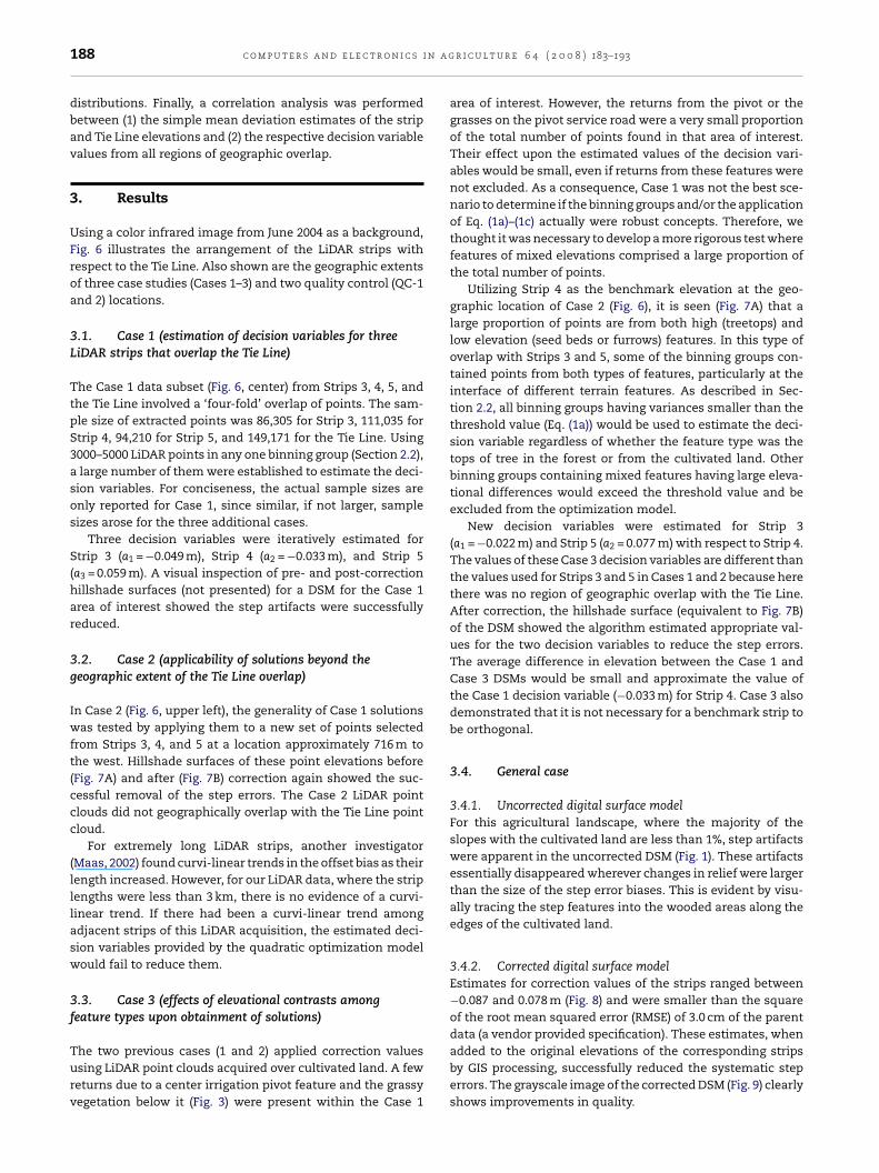

i n a g

188 c o m p u t e r s a n d e l e c t r o n i c s

distributions. Finally, a correlation analysis was performedbetween (1) the simple mean deviation estimates of the stripand Tie Line elevations and (2) the respective decision variablevalues from all regions of geographic overlap.

3. Results

Using a color infrared image from June 2004 as a background,Fig. 6 illustrates the arrangement of the LiDAR strips withrespect to the Tie Line. Also shown are the geographic extentsof three case studies (Cases 1–3) and two quality control (QC-1and 2) locations.

3.1. Case 1 (estimation of decision variables for threeLiDAR strips that overlap the Tie Line)

The Case 1 data subset (Fig. 6, center) from Strips 3, 4, 5, andthe Tie Line involved a ‘four-fold’ overlap of points. The sam-ple size of extracted points was 86,305 for Strip 3, 111,035 forStrip 4, 94,210 for Strip 5, and 149,171 for the Tie Line. Using3000–5000 LiDAR points in any one binning group (Section 2.2),a large number of them were established to estimate the deci-sion variables. For conciseness, the actual sample sizes areonly reported for Case 1, since similar, if not larger, samplesizes arose for the three additional cases.

Three decision variables were iteratively estimated forStrip 3 (a1 = −0.049 m), Strip 4 (a2 = −0.033 m), and Strip 5(a3 = 0.059 m). A visual inspection of pre- and post-correctionhillshade surfaces (not presented) for a DSM for the Case 1area of interest showed the step artifacts were successfullyreduced.

3.2. Case 2 (applicability of solutions beyond thegeographic extent of the Tie Line overlap)

In Case 2 (Fig. 6, upper left), the generality of Case 1 solutionswas tested by applying them to a new set of points selectedfrom Strips 3, 4, and 5 at a location approximately 716 m tothe west. Hillshade surfaces of these point elevations before(Fig. 7A) and after (Fig. 7B) correction again showed the suc-cessful removal of the step errors. The Case 2 LiDAR pointclouds did not geographically overlap with the Tie Line pointcloud.

For extremely long LiDAR strips, another investigator(Maas, 2002) found curvi-linear trends in the offset bias as theirlength increased. However, for our LiDAR data, where the striplengths were less than 3 km, there is no evidence of a curvi-linear trend. If there had been a curvi-linear trend amongadjacent strips of this LiDAR acquisition, the estimated deci-sion variables provided by the quadratic optimization modelwould fail to reduce them.

3.3. Case 3 (effects of elevational contrasts amongfeature types upon obtainment of solutions)

The two previous cases (1 and 2) applied correction valuesusing LiDAR point clouds acquired over cultivated land. A fewreturns due to a center irrigation pivot feature and the grassyvegetation below it (Fig. 3) were present within the Case 1

r i c u l t u r e 6 4 ( 2 0 0 8 ) 183–193

area of interest. However, the returns from the pivot or thegrasses on the pivot service road were a very small proportionof the total number of points found in that area of interest.Their effect upon the estimated values of the decision vari-ables would be small, even if returns from these features werenot excluded. As a consequence, Case 1 was not the best sce-nario to determine if the binning groups and/or the applicationof Eq. (1a)–(1c) actually were robust concepts. Therefore, wethought it was necessary to develop a more rigorous test wherefeatures of mixed elevations comprised a large proportion ofthe total number of points.

Utilizing Strip 4 as the benchmark elevation at the geo-graphic location of Case 2 (Fig. 6), it is seen (Fig. 7A) that alarge proportion of points are from both high (treetops) andlow elevation (seed beds or furrows) features. In this type ofoverlap with Strips 3 and 5, some of the binning groups con-tained points from both types of features, particularly at theinterface of different terrain features. As described in Sec-tion 2.2, all binning groups having variances smaller than thethreshold value (Eq. (1a)) would be used to estimate the deci-sion variable regardless of whether the feature type was thetops of tree in the forest or from the cultivated land. Otherbinning groups containing mixed features having large eleva-tional differences would exceed the threshold value and beexcluded from the optimization model.

New decision variables were estimated for Strip 3(a1 = −0.022 m) and Strip 5 (a2 = 0.077 m) with respect to Strip 4.The values of these Case 3 decision variables are different thanthe values used for Strips 3 and 5 in Cases 1 and 2 because herethere was no region of geographic overlap with the Tie Line.After correction, the hillshade surface (equivalent to Fig. 7B)of the DSM showed the algorithm estimated appropriate val-ues for the two decision variables to reduce the step errors.The average difference in elevation between the Case 1 andCase 3 DSMs would be small and approximate the value ofthe Case 1 decision variable (−0.033 m) for Strip 4. Case 3 alsodemonstrated that it is not necessary for a benchmark strip tobe orthogonal.

3.4. General case

3.4.1. Uncorrected digital surface modelFor this agricultural landscape, where the majority of theslopes with the cultivated land are less than 1%, step artifactswere apparent in the uncorrected DSM (Fig. 1). These artifactsessentially disappeared wherever changes in relief were largerthan the size of the step error biases. This is evident by visu-ally tracing the step features into the wooded areas along theedges of the cultivated land.

3.4.2. Corrected digital surface modelEstimates for correction values of the strips ranged between−0.087 and 0.078 m (Fig. 8) and were smaller than the squareof the root mean squared error (RMSE) of 3.0 cm of the parentdata (a vendor provided specification). These estimates, when

added to the original elevations of the corresponding stripsby GIS processing, successfully reduced the systematic steperrors. The grayscale image of the corrected DSM (Fig. 9) clearlyshows improvements in quality.

c o m p u t e r s a n d e l e c t r o n i c s i n a g r i c u l t u r e 6 4 ( 2 0 0 8 ) 183–193 189

Fig. 7 – Hillshade of the digital surface model for the Case 2 and 3 areas of interest. Panel A shows the step artifacts beforec rtifacts after adding the decision variable corrections to theL

Hash

FCt1

orrection. Panel B indicates successful removal of the step aiDAR points.

The elevation range of the DSM is approximately 44–81 m

AE (height above the ellipsoid), where the higher elevationsre the tops of trees, and spanned a 638.2-ha agricultural land-cape. During acquisition, the LiDAR strips were planned toave a 3-fold overlap for each unit of surface area across this

ig. 8 – Bar graph depicting the magnitudes of the Generalase decision variables for each LiDAR strip estimated by

he optimization model. No estimate was obtained for Strip.

Fig. 9 – Grayscale image of the digital surface model afterapplication of the step error corrections. Compare to Fig. 1.

area of interest, which provided a data density great enoughto build a DSM at a spatial resolution of 0.5 m.

3.5. Quality control (QC) assessments

A subset of the unadjusted DSM (Fig. 10) was extracted fromthe location labeled QC-1 (Fig. 6). A visual examination of thisraster surface subset indicates lower elevations (dark gray orblack) generally occur to the southwest; a higher elevation(white) ridge rises from the center and runs to the northeast,while an indistinct drainage feature runs north to south alongthe western edge. Along the bottom eastern half, alternating

dark gray (lower elevations) and lighter gray (higher elevations)bands run parallel to one another in an east–west orientation.The feature in the extreme southwest corner are the tops oftrees.

190 c o m p u t e r s a n d e l e c t r o n i c s i n a g r i c u l t u r e 6 4 ( 2 0 0 8 ) 183–193

Fig. 10 – Grayscale image of a subset of the uncorrectedDSM for the quality control site QC-1 (see Fig. 6). Note the

Fig. 12 – Profile plot of the uncorrected strips with respectto the Tie Line viewed by the Easting co-ordinate for thequality control site QC-2. The sharp dip on the right is thedrainage feature visible just beneath the middle pivotsection in Fig. 3. Linear splines were fit to the point clouds

blurred appearance of drainage features, roadways andtillage patterns.

For the same geographic location, Fig. 11 shows how thepost-processing of the original LiDAR point clouds reducedthe step artifacts and improved the quality of the DSM. Theappearance of this surface is less blurred and various featuresare more distinctive. While the major features of the south-westerly basin and northeasterly ridge are still seen, it is nowobvious that the north–south drainage feature along the west-ern edge consisted of two parallel lines of different widths.Inspection on site showed this to be a drainage feature builtby a tractor drawn implement that created two parallel ditchesto improve surface drainage. The western cut received more

water erosion than the eastern cut, causing it to widen withtime.

The east–west bands lying parallel to one another along theeastern quadrant of the bottom half of both the uncorrected

Fig. 11 – Grayscale image of a subset of the corrected DSMfor the quality control site QC-1 (see Fig. 6). Note theincreased clarity of drainage features, roadways and tillagepatterns. Compare to Fig. 10.

of each strip for additional clarity.

and corrected DSMs (Figs. 10 and 11) are the results of longterm tillage operations. These parallel bands are not as dis-tinct in the northern part of these DSM subsets, because theslope of the land there is gentler, reducing the water flow rate.In contrast, the slope increases east to west moving towardthe south to produce the darker bands at approximately 10 mspacings, where tillage passes by eight-row equipment abutone another. A probable explanation for these parallel bandsis that the rate of erosion is greater along the margins thanthe middle of the tillage passes. Parallel patterns correspond-ing to tillage operations are found throughout the correctedDSM (see also Fig. 7B).

Profile plots from a second location labeled QC-2 (Fig. 6)provided another examination of the optimization model’sability to estimate decision variables to alleviate step errors.The before (Figs. 12 and 13) and after (Figs. 14 and 15) profileplot comparisons for Strips 4–6 clearly indicate reductions instep error magnitudes. These effects are highlighted by splinelines fit to the different point clouds. The closely spaced pointsoccurring as linear patterns in the profile plots viewed alongthe Easting co-ordinates (Figs. 12 and 14) belong to similar scanlines within the strips. The remaining width of the point cloudprofiles for these lateral views of the point clouds in the Eastingand Northing directions, even after correction, is due primar-ily to the alternating undulation of the crop seed bed and thefurrows (Fig. 2), and/or returns from the grassy vegetation ofthe center pivot service road (Fig. 3). Returns from the centerpivot itself (Fig. 3) have been excluded from all profile plots toenhance the scaling of the y-axis.

4. Discussion

Case 1 estimates for Strips 3, 4, and 5 (Section 3.1) were slightlydifferent than their corresponding estimates in the General

c o m p u t e r s a n d e l e c t r o n i c s i n a g r i c u l t u r e 6 4 ( 2 0 0 8 ) 183–193 191

Fig. 13 – Profile plot of the uncorrected strips with respectto the Tie Line viewed by the Northing co-ordinate. Notetc

Cbal5ltab

r(d

Ftqbts

Fig. 15 – Profile plot of the uncorrected strips with respectto the Tie Line viewed by the Northing co-ordinate. Notethe removal of the obvious step error discrepancies among

he obvious step error discrepancy between the point

louds of Strips 4 and 6.

ase (Fig. 8). An explanation is the fact that these strips had toe reconciled to other adjoining strips that were to the northnd south of them. For example, Strip 3 geographically over-apped Strip 2 at the same time it overlapped Strip 4. Strip

geographically overlapped Strip 6 at the same time it over-apped with Strip 4, and so on. We demonstrated in Case 1hat the optimization model concurrently works with sets ofdjoining strips. Strips 2 and 6 were excluded during Case 1,ut were included in the General Case application.

The removal of the step errors as shown in the cor-ected DSM (Fig. 9) and the quality control illustrationsFigs. 11, 14 and 15) were due to the addition of the estimatedecision variable values to the elevation attribute of each point

ig. 14 – Profile plot of the corrected strips with respect tohe Tie Line viewed by the Easting co-ordinate for theuality control site QC-2. The point clouds of the stripsetter conform to the elevations of the Tie Line in contrasto Fig. 12. Linear splines were fit to the point clouds of eachtrip for additional clarity.

the point clouds of the strips in comparison to Fig. 13.

of the respective LiDAR strip. No additional smoothing or focalprocessing (Chang, 2006; Theobald, 2003) algorithms wereapplied while building the corrected DSM with the adjustedelevation values of the LiDAR point clouds.

One supplemental benefit of our processing efforts was thediscovery of a source of random error in these data. Vary-ing point density (Fig. 16) due to geographic gaps betweenadjoining strips also created linear features at some locationswhich primarily show up as textural differences in the cor-rected DSM. The locations of a few gaps due to this cause wereeasily found by visual inspection of the hillshade image of cor-rected elevations (not shown). The effect of gap errors wasmost severe wherever the distance between adjacent LiDARstrips exceeded 4 m. Thus, this corrected DSM will requireadditional GIS processing in those areas wherever the pointsample intensity varied due to gaps of random widths. Hu andTao (2005) and Filin and Pfeifer (2005) discussed processingLiDAR data that vary in point density.

Whenever homogenous areas of flat terrain are unavailableit is not possible to optimally estimate simple mean devia-tions between strips. When a common geographical area is notflat, effects of scan angle and rate, reflectance signatures, anddirection of strip acquisition (Burman, 2002; Morin, 2002) affectthe frequency distribution of point elevations from differentstrips (Fig. 17). On non-flat terrain, these cumulative effectsdetermine the shape of the frequency distribution of eleva-tion attributes of the different strips obtained from a commonarea of geographic overlap and influence the estimates of theirrespective mean elevations. As a consequence, the differencebetween the strip means for areas of geographic overlap willnot optimally estimate the size of the step error bias. Thesecomparative histograms also demonstrate that LiDAR eleva-tion data from homologous, non-flat, areas are not normally

distributed. An optimization model methodology that seeksto minimize the among-strip variance will perform better(Ignizio, 1982) when all these types of influences arise.

192 c o m p u t e r s a n d e l e c t r o n i c s i n a g r i c u l t u r e 6 4 ( 2 0 0 8 ) 183–193

Fig. 16 – Illustration of gap (or sampling intensity, Panel A) errors between Strips 10 and 12 at a selected location along theirlengths. This type of random error may cause textural differences in the digital surface model after step error biases are

en S

corrected. Panel B shows the absence of the gap error betwebetween them as shown in the detailed views.

To further examine this issue, estimates of simple meandeviations of the thirteen strips and the Tie Line elevationsacross the fullest possible extent of the various geographicoverlaps were obtained. A correlation analysis between therespective decision variables and simple differences betweenthe mean estimates of the strips and Tie Line found anon-significant correlation of −0.26 (P = 0.4214). This resultillustrates the difficulty of estimating mean strip deviations byalgebraic methods for agricultural landscapes. Therefore, themajor benefit of this optimization model approach was the

estimation of correction constants without the requirementfor highly planar and homologous planar features.

In conclusion, the corrected DSM of the agricultural land-scape was accepted as an accurate representation of relative

Fig. 17 – Comparative histograms of point elevations in theregion of overlap between Strip 5 and the Tie Line beforeremoving the step error. A small number of returns fromthe center pivot (see Fig. 3) between elevations of 48–52 mwere excluded for clarity.

r

trips 10 and 12 at another location. Strip 11 is centered

elevation since drainage patterns, tree heights, building rela-tionships, etc. corresponded to features observed on site.Any remaining error due to the vertical bias of the TieLine itself to the actual elevations of this landscape islikely to be small since the RMSE (3.0 cm) of the unad-justed data was also small. The quadratic optimization modelapproach successfully reduced systematic step errors of smallmagnitudes.

Acknowledgements

Financial support was provided by Advanced Spatial Tech-nologies for Agriculture (ASTA-322-298) and the USDAArea-Wide Tarnished Plant Bug Management Project (thruARS CRIS Project 6406-21610-006-00D). Additional funding wasprovided by the USDA-ARS Genetics and Precision Agricul-ture Research Unit, Mississippi State, MS (ARS CRIS Project6406-21610-007-00D). Appreciation is expressed to Dr. R.O.Bowden, Department of Industrial and Systems Engineering,Mr. Ronald E. Britton, USDA-ARS, Genetics and Precision Agri-culture Research Unit, Mississippi State, Dr. D.B. Reynolds,Department of Plant and Soil Sciences, Mississippi State, MS,and Mr. Kenneth Hood, Perthshire Farms, Gunnison, MS, fortheir support. Approved for publication as Journal Article No. J-10876 of the Mississippi Agricultural and Forestry ExperimentStation, Mississippi State University.

e f e r e n c e s

Ackermann, F., 1999. Airborne laser scanning—present statusand future expectations ISPRS. Journal of PhotogrammetryRemote Sensing 54, 64–67.

a g r

A

B

B

B

C

C

E

E

F

F

F

F

H

H

H

H

I

J

K

K

L

Willers, J.L., Milliken, G.A., O’Hara, C.G., Jenkins, J.N., 2004.

c o m p u t e r s a n d e l e c t r o n i c s i n

xelsson, P., 1999. Processing of laser scanning data-algorithmsand applications. ISPRS Journal of Photogrammetry RemoteSensing 54, 138–147.

altsavias, E.P., 1999. Airborne laser scanning: basic relations andformulas. ISPRS Journal of Photogrammetry Remote Sensing54, 199–214.

arnes, F.J., Karl, R.J., Kunkel, K.E., Stone, G.L., 1990. Lidardetermination of horizontal and vertical variability in watervapor over cotton. Remote Sensing of Environment 32, 81–90.

urman, H., 2002. Laser strip adjustment for data calibration andverification. International Archives of Photogrammetry andRemote Sensing 34 (3), 67–72.

hang, K., 2006. Introduction to Geographic Information Systems,3rd ed. McGraw Hill, Boston, MA.

rombaghs, M.J.E., Brugelmann, R., de Min, E.J., 2000. On theadjustment of overlapping strips of laser altimeter heightdata. International Archives of Photogrammetry and RemoteSensing 33 (B3/1), 230–237.

SRI, 1998. ESRI Shapefile Technical Description. ESRI, Redlands,CA.

SRI, 2005. Arc Hydro Tools Overview, Version 1.1. ESRI, Redlands,CA.

ilin, S., 2003. Recovery of systematic biases in laser altimetrydata using natural surfaces. Photogrammetric Engineering &Remote Sensing 69 (11), 1235–1242.

ilin, S., 2004. Surface classification from airborne laser scanningdata. Computers & Geosciences 30, 1033–1041.

ilin, S., Pfeifer, N., 2005. Neighborhood systems for airbornelaser data. Photogrammetric Engineering & Remote Sensing71 (6), 743–755.

ritsch, D., Kilian, J., 1994. Filtering and calibration of laserscanner measurements. International Archives ofPhotogrammetry and Remote Sensing 30 (3), 227–234.

immelblau, D.M., 1972. Applied Nonlinear Programming.McGraw-Hill, New York.

ollaus, M., Wagner, W., Kraus, K., 2005. Airborne laser scanningand usefulness for hydrological models. Advances inGeosciences 5, 57–63.

u, Y., Tao, C.V., 2005. Hierarchical recovery of digital terrainmodels from single and multiple return lidar data.Photogrammetric Engineering & Remote Sensing 71 (4),425–433.

uising, E.J., Pereira, L.M., 1998. Errors and accuracy estimates oflaser data acquired by various laser scanning systems fortopographic applications. ISPRS Journal of PhotogrammetryRemote Sensing 53 (5), 245–261.

gnizio, J.P., 1982. Linear Programming in Single- & MultipleObjective Systems. Prentice-Hall, Englewood Cliffs, NewJersey.

ensen, J.R., 2000. Remote Sensing of the Environment: An EarthResource Perspective. Prentice-Hall, New Jersey, pp. 285–332.

ager, H., 2004. Discrepancies between overlapping laser scannerstrips—simultaneous fitting of aerial laser scanner strips. In:International Archives of Photogrammetry and RemoteSensing, Proceedings of the XX ISPRS Congress, Istanbul,Turkey, July 12–23 (CD-ROM).

raus, K., Pfeifer, N., 1998. Determination of terrain models in

wooded areas with airborne laser scanner data. ISPRS Journalof Photogrammetry Remote Sensing 53 (4), 193–203.

atypov, D., 2002. Estimating relative lidar accuracy informationfrom overlapping flight lines. ISPRS Journal ofPhotogrammetry Remote Sensing 56, 236–245.

i c u l t u r e 6 4 ( 2 0 0 8 ) 183–193 193

Leyva, R.I., Henry, R.J., Graham, L.A., Hill, J.M., 2002. Use of LiDARto determine vegetation vertical distribution in areas ofpotential black-capped vireo habitat at Fort Hood, Texas.Endangered Species Monitoring and Management at FortHood, Texas, 2002 Annual Report. The Nature Conservancy,Fort Hood, TX.

Luethy, L., Ingensand, H., 2001. How to evaluate the quality ofairborne laser scanning data. International ArchivesPhotogrammetry, Remote Sensing Spatial InformationSciences XXXVI (8/W2), 313–317.

Maas, H., 2002. Methods for measuring height and planimetrydiscrepancies in airborne laserscanner data. PhotogrammetricEngineering & Remote Sensing 68 (9), 933–940.

Means, J.E., Acker, S.A., Fitt, B.J., Renslow, M., Emerson, L.,Hendrix, C.J., 2000. Predicting forest stand characteristics withairborne scanning LiDAR. Photogrammetric Engineering &Remote Sensing 54, 95–104.

Morin, K.W., 2002. Calibration of airborne laser scanners. UCGEReports No. 20179, Department of Geomatics Engineering,University of Calgary, Calgary, Alberta, CA [URL:http://www.geomatics.ucalgary.ca/links/GradTheses.html](Verified 20 March 2007).

Pfeifer, N., 2005. Airborne laser scanning strip adjustment andautomation of tie surface measurement. Boletim de CienciasGeodesicas 11 (1), 3–22.

Popescu, S.C., Wynne, R.H., Nelson, R.F., 2002. Estimatingplot-level tree heights with lidar: local filtering with acanopy-height based variable window size. Computers andElectronics in Agriculture 37, 71–95.

Schuckman, K., 2003. Announcement of the proposed ASPRSbinary lidar data file format standard. PhotogrammetricEngineering & Remote Sensing 69 (1), 13–19.

Shan, J., Sampath, A., 2005. Urban DEM generation from raw lidardata: a labeling algorithm and its performance.Photogrammetric Engineering & Remote Sensing 71 (2),217–226.

Sithole, G., Vosselman, G., 2004. Experimental comparison offilter algorithms for bare-earth extraction from airborne laserscanning point clouds. ISPRS Journal of Photogrammetry andRemote Sensing 59, 85–101.

Skaloud, J., Lichti, D., 2006. Rigorous approach to bore-sightself-calibration in airborne laser scanning. ISPRS Journal ofPhotogrammetry and Remote Sensing 61, 47–59.

Theobald, D.M., 2003. GIS Concepts and ArcGIS® Methods.Conservation Planning Technologies. Fort Collins, CO.

Vosselman, G., 2002. On the estimation of planimetric offsets inlaser altimetry data. International Archives ofPhotogrammetry Remote Sensing 34 (3A), 375–380.

Wehr, A., Lohr, U., 1999. Airborne laser scanning—anintroduction and overview. ISPRS Journal of PhotogrammetryRemote Sensing 54, 68–82.

Willers, J.L., Milliken, G.A., Jenkins, J.N., O’Hara, C.G., Gerard, P.D.,Reynolds, D.B., Boykin, D.L., Good, P.V., Hood, K.B., 2008.Defining the experimental unit for the design and analysis ofsite-specific experiments in commercial cotton fields.Agricultural Systems 96, 237–249.

Information technologies and the design and analysis ofsite-specific experiments within commercial fields. In:Proceedings of the 16th Applied Statistics in AgricultureConference, Manhattan, Kansas, pp. 41–73.