Department of Economics and Marketing Discussion Paper No.19

A Portfolio Choice Model of the Demand for Recreational Trips

Richard S Tay Patrick S McCarthy

Jerry J Fletcher

July 1996

Department of Economics and Marketing PO Box 84

Lincoln University CANTERBURY

Telephone No: (64) (3) 325 2811

Fax No: (64) (3) 325 3847 E-mail: Williaml@lincoln.ac.nz

ISSN 1173-0854

ISBN 0-9583485-6-1

Richard S Tay Department of Economics and Marketing P O Box 84, Lincoln University Canterbury, New Zealand Patrick S McCarthy Department of Economics Purdue University West Lafayette, IN 47907, USA Jerry J Fletcher Division of Resource Management West Virginia University Morgantown, WV 26506, USA Support for this research was provided for by the Department of Economics and the Department of Agricultural Economics, Purdue University, by a cooperative agreement between Purdue University and the US Department of Agriculture, Soil Conservation Service, and by the Division of Resource Management, West Virginia University.

Contents

List of Tables (i)

1. Introduction 1

2. Recreational Portfolio Choice Model 2

3. Sampling of Alternatives 6

4. Sampling Correction 7

5. Data 10

6. Estimation Results 13

7. Choice Elasticities 14

8. Summary 15

References 18

List of Tables

1. Distribution of Trips 20

2. Distribution of Anglers’ Characteristics by Strata 21

3. Description of Explanatory Variables 22

4. Estimation Results 23

5. Choice Elasticities 24

(i)

1. Introduction

A fully specified model of household recreational demands per time period includes five

interrelated travel decisions corresponding to choice of destination, duration and frequency of

trips, travel mode, and trip timing. Because of the complexity involved in specifying the

relationships among the decision components, existing research in this area has reduced the

scope of the problem by adopting (explicitly or implicitly) various simplifying assumptions.

Most studies have focused on a single decision. Ribaudo et al. (1984), Smith (1988), and

Smith and Kaoru (1986) focused on frequency choice; Kealy and Bishop (1986) estimated

the total time spent at a site; and Tay and McCarthy (1994) analysed destination choice

decisions. A few studies, however, have estimated multi-dimensional nested models of

destination, duration and frequency choices. Brown (1979) estimated a three stage nested

logit model in which destination choice is conditioned upon the choice of duration which, in

turn, is conditioned upon frequency choice. Caulkins et al. (1986) estimated a nested logit

model of destination choice conditioned upon taking a trip. Bockstael et al. (1984) estimated

a nested logit model of destination choice conditioned upon fresh/salt water recreation.

The nested structure, however, has several limitations. Since there may potentially be many

different choice structures consistent with random utility maximisation, the analyst must

often decide which structure is best. Also, since these models are typically estimated

sequentially rather than by full maximum likelihood methods, the coefficient estimates are

not asymptotically efficient. Moreover, using parameter estimates from lower branches to

define inclusive values in upper branches introduces errors which cumulate upwards and can

become quite serious beyond 3 stages (Ben-Akiva and Lerman, 1985).

Although not in the recreational demand literature, some models avoided the problem of

identifying structures by forming individual portfolios that encompass several choice

dimensions. In an analysis of trip chaining, Adler and Ben-Akiva (1979) defined the choice

alternatives as travel tours that included destination, frequency, and modal decisions. More

recently, Train et al. (1987) and Atherton et al. (1990) developed a portfolio model of local

residential telephone demands which included destination, duration, frequency, and the

timing of calls.

1

In the spirit of Train et al. (1987) and Atherton et al. (1990), this paper develops a discrete

choice model of the annual demand for freshwater fishing using data collected by the 1985

Survey of Fishing, Hunting, and Wildlife-Associated Recreation (Bureau of Census,

1987a,b). This study extends previous recreational demand research by defining an annual

portfolio of recreational trips as the elemental alternative. There are three distinct advantages

to this approach. First, identifying an angler's choice alternative as a portfolio of recreational

trips greatly facilitates a multidimensional analysis of destination, frequency, and duration of

angling trips, the most important aspects of recreational fishing. Second, focusing upon an

angler's annual portfolio avoids the need to model the effect that trips taken in one part of the

year have upon one's ability to make trips at other times in the year. Third, in contrast to the

sequential estimation of a multidimensional structure, a portfolio approach eliminates the

"cumulative errors" concern associated with introducing estimated inclusive values at lower

levels of a nest into the upper branches.

2. Recreational Portfolio Choice Model

A major departure of this analysis from other multidimensional studies of recreational fishing

is the assumption that consumers plan their annual recreational travel schedules at the

beginning of each period. This implies that a consumer chooses a recreational fishing

portfolio i from the available set of portfolios which describes how many trips of different

durations are to be made to each destination in the period. Thus, the frequency, duration, and

destinations of fishing trips are jointly modelled.

Define portfolio i as:

(1) i = (N N Nirdi

RDi

11, , , , ) i = 1 , ... ,

where r indexes the region visited (r = 1, 2, ... , R);

d indexes the duration of the trip (d = 1, 2, ... , D); and

Nrdi represents the number of trips to region r of duration d in portfolio i.

2

One example of a portfolio is i = ( 511, 0, ... , 123, 0,...,0RD ) which is a travel package

consisting of five one day trips to region 1 and one three day trip to region 2. Another

portfolio may be

j = (0, ... , 3041 , 0, ... , 0RD) which consists of thirty one day trips to region 4 and

no visits to any other region.

Let c be the set of all possible portfolios available to consumer c. A consumer is assumed

to select from c the portfolio that yields the highest utility as reflected by one's indirect

utility function. In general, the consumer's indirect utility for a given portfolio, ( i c ),

comprises two components: a positive component, , which reflects the indirect utility

associated with fishing trips of varying lengths to alternative destinations and a negative

component, C which reflects the cost associated with these trips.

Vci

ci

ci

V = V( Trips' Attractiveness, Trips' Cost ) ci

(2) = V( , C ) ic ci

ci

Let rlc represent the positive component of consumer c's indirect utility for a single one day

trip to region r. Since trips of longer lengths are assumed to yield higher utility, the indirect

utility to region r of duration d is assumed to be the product of the utility for a one day trip

and trip duration, (d)(rlc). Thus, N trips of duration d taken by consumer c to region r in

portfolio i yields utility

rdci

= ( ) (d) (rlc) ic rdci N rdc

i

Note that this specification assumes that the positive component of indirect utility is linear in

duration and number of trips which can be relaxed whenever necessary. In particular, a more

general specification would specify trip frequency and duration to reflect diminishing

marginal utility. However, in preliminary runs of the model, specifications which reflected

diminishing utility in these trip components generally led to inferior fits. Summing over all

trips included in the portfolio gives the attractiveness of portfolio i;

3

(3) ic ci

rci

rlcr

TS ( )

)

))

where T is the total time in portfolio i spent at region r by consumer c. S N drci

rdci

d ( )( )

In addition to the positive benefits received from fishing activities, consumer c will incur a

cost, , to access the fishing sites in portfolio i. Denoting by Crc the per trip cost of

consumer c to region r and recognising that this cost is generally not dependent upon trip

duration, total costs to region r can be expressed as the product of Crc and the total number of

trips in portfolio i to the region, . Summing over the different regions gives the total

access cost of the trips in portfolio i;

Cci

N rci

(4) ic C Cci

rcr

N rci (

Thus, a consumer's indirect utility associated with portfolio i can be expressed as

(5) V = V( , ) ci c

i Cci

= V ic TS N Crci

rlcr

rci

rcr

( ( ), (

For this study, and consistent with most random utility models of discrete choice, we shall

adopt the assumption that indirect utility is additively separable. Specifically, we assume that

the indirect utility rlc associated with a one day trip to region r is a linear function,

k krck

Z , of observed socio-economic characteristics of consumer c as well as observed

attributes of the region r. In addition, we assume that the cost per trip to region r is

proportional to the distance Krc from region r to consumer c's region of origin. The indirect

utility that consumer c receives from portfolio i is then given by

V = r [ ( ) ( c

i TSrci k

kkrcZ ) ] ( Krc) N rc

i

r

4

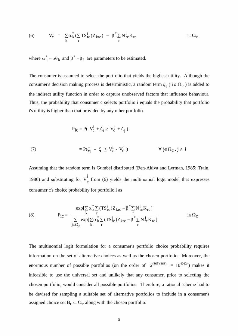
(6) = ic Vci k rc

ikrc

rkTS Z* ( ) )

k

* N Krci

rcr

where and are parameters to be estimated. k* *

The consumer is assumed to select the portfolio that yields the highest utility. Although the

consumer's decision making process is deterministic, a random term i ( i c ) is added to

the indirect utility function in order to capture unobserved factors that influence behaviour.

Thus, the probability that consumer c selects portfolio i equals the probability that portfolio

i's utility is higher than that provided by any other portfolio.

Pic = P( + Vci i > +Vc

j j )

(7) = P( j i < - ) jc , j i Vci Vc

j

Assuming that the random term is Gumbel distributed (Ben-Akiva and Lerman, 1985; Train,

1986) and substituting for Vic from (6) yields the multinomial logit model that expresses

consumer c's choice probability for portfolio i as

(8) Pic =

exp[ ( ) ]

exp[ ( ) ]

* *

* *

kk

rci

krc rci

rrc

r

kk

rcj

krc rcj

rrc

rj

TS Z N K

TS Z N Kc

ic

The multinomial logit formulation for a consumer's portfolio choice probability requires

information on the set of alternative choices as well as the chosen portfolio. Moreover, the

enormous number of possible portfolios (on the order of 2(365)(368) = 1040434) makes it

infeasible to use the universal set and unlikely that any consumer, prior to selecting the

chosen portfolio, would consider all possible portfolios. Therefore, a rational scheme had to

be devised for sampling a suitable set of alternative portfolios to include in a consumer's

assigned choice set Bc c along with the chosen portfolio.

5

3. Sampling of Alternatives

The 1985 Survey of Fishing, Hunting, and Wildlife-Associated Recreation identifies 368

destination regions or zones in the U.S. and provides information on the number of trips in

three duration categories; one day, two days and three or more days. Respondents were

asked to identify up to nine destinations visited and provide detailed information for up to

five destinations. While potentially limiting, this does not represent a major practical

restriction since 99.8 percent of the Indiana respondents, the sample considered in this study,

visited five or fewer zones. Thus, in this study, a consumer's portfolio will include a

maximum of fifteen destination-duration elements corresponding to the three duration

categories and the five destinations for which detailed information was available.

Recognising that recreational fishermen, responding to time and budget constraints, are less

likely to consider farther destinations than nearer sites, a stratified importance sampling

methodology (Ben-Akiva and Lerman, 1985) was adopted for selecting destinations to

include in each portfolio. In particular, a portfolio was constructed to include the origin zone

of the consumer together with two zones from contiguous regions and two zones from non-

contiguous outer areas. Due to confidentiality restrictions imposed by the Bureau of the

Census, the origin zone may be defined to include more than one destination zone. Since

98.5 percent of Indiana anglers selected two or fewer contiguous zones and only 1 percent

visited at most two outer regions, assigning lower selection probabilities to regions further

from one's origin yields alternative portfolios that more closely reflect observed choices.

Also note that this represents an upper limit on the number of regions included in a portfolio

since the number of trips taken to any of the five included zones may be zero.

The next step in building consumer portfolios was to determine the number and allocation of

trips to each of the 15 destination-duration pairs in an alternative portfolio. A logical

procedure is to segment the sample by destination-duration pair, fit the observed data to some

known distributions and randomly sample from the fitted distributions - an approach adopted

by Train et al. (1987) and Atherton et al. (1990). However, since only a small proportion of

the trips were taken to outer zones and a very small percentage of the trips were of three or

more days, reasonable fits for some distributions were difficult to obtain. Therefore, a

modified procedure was used. First, the observed number of trips by all households was used

6

to fit a distribution for total trip frequencies, , Next, each household was assigned a

number of trips by a random draw from this distribution. Last, the sampled number of trips

was allocated to the fifteen destination-duration pairs according to the relative frequencies

observed in the data.

N t

Several common distributions, including the normal, Poisson, chi-square, and exponential,

were considered and fitted against the data. Sample statistics for the number of trips were

computed from the data and used as the required moments for the proposed distributions of

the total number of trips. Similar to Train et al. (1987) and Atherton, et al. (1990), the

exponential distribution with a mean of 22.5 (sample average) provided the best fit and was

adopted as the sampling distribution in this study. Figure 1 plots the actual distribution

against the exponential distribution with a mean of 22.5.

As noted above, a total number of trips for consumer c, , was sampled from the

exponential distribution then distributed among the fifteen destination/duration combinations

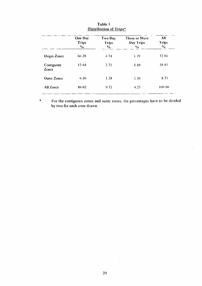
based upon the relative sample frequencies observed in the data (see Table 1). As an

example of this procedure, since the relative frequency of one day trips to the origin zone

represented 66.28 percent of all trips taken, if 30 trips are drawn from the exponential

distribution, then 20 trips ((30)(0.6628)) will be randomly assigned as one day trips to the

origin.

N tc

The above sampling procedures (sampling of destinations and frequencies) were repeated to

obtain 9 alternative portfolios for each observation. Together with the portfolio actually

chosen, each consumer's assigned choice set, Bc, contains 10 portfolios.

4. Sampling Correction

Since only a subset, Bc, of the universal set, c, is used in estimation, it is necessary to

account for the possible bias introduced by the sampling of alternatives (Ben-Akiva and

Lerman, 1985). Let P(Bci) be the conditional probability of sampling the subset Bc given

that the chosen portfolio is i. Then, the conditional probability of choosing portfolio i given

choice set Bc is

7

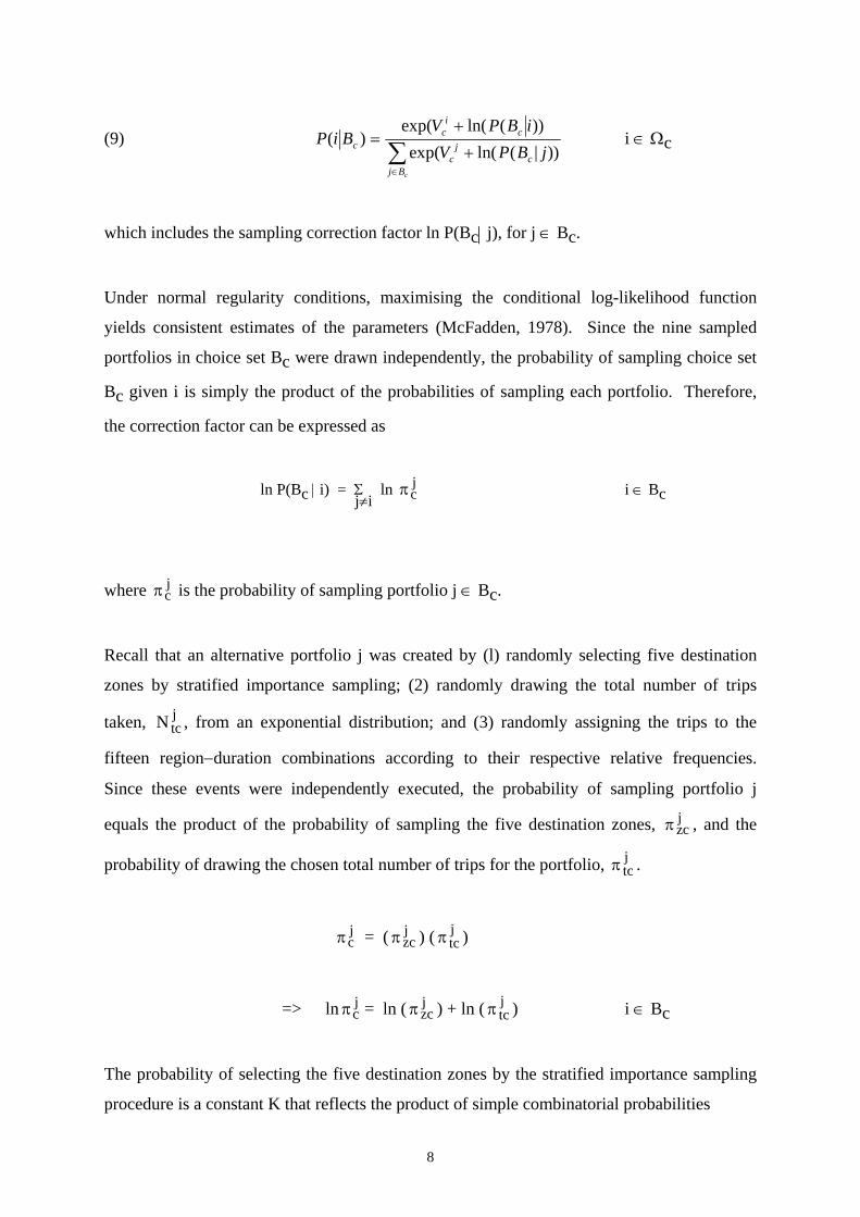
(9) P i BV P B i

V P Bcci

c

cj

cj Bc

( )exp( ln( ( ))

exp( ln( ( | ))

j

i c

which includes the sampling correction factor ln P(Bcj), for j Bc.

Under normal regularity conditions, maximising the conditional log-likelihood function

yields consistent estimates of the parameters (McFadden, 1978). Since the nine sampled

portfolios in choice set Bc were drawn independently, the probability of sampling choice set

Bc given i is simply the product of the probabilities of sampling each portfolio. Therefore,

the correction factor can be expressed as

ln P(Bci) = ji

ln i Bc

cj

where is the probability of sampling portfolio j Bc. cj

Recall that an alternative portfolio j was created by (l) randomly selecting five destination

zones by stratified importance sampling; (2) randomly drawing the total number of trips

taken, , from an exponential distribution; and (3) randomly assigning the trips to the

fifteen regionduration combinations according to their respective relative frequencies.

Since these events were independently executed, the probability of sampling portfolio j

equals the product of the probability of sampling the five destination zones, , and the

probability of drawing the chosen total number of trips for the portfolio, .

N tcj

zcj

tcj

= ( ) ( ) cj zc

j tcj

=> ln = ln ( ) + ln ( ) i Bc cj zc

j tcj

The probability of selecting the five destination zones by the stratified importance sampling

procedure is a constant K that reflects the product of simple combinatorial probabilities

8

(10) = zcj 1 2 1

1

2 1

11 2 2 3 3M M M M M

( )( )

( )( )

( )( )

( )( )

= K

where Ml = Number of zones in the origin stratum, M2 = Number of zones in the contiguous

stratum, and M3 = number of zones in the outside stratum.

The probability of drawing a total number of trips for portfolio j, given that the exponential

distribution was used for sampling, is computed using the cumulative distribution (Gt) of the

exponential variate with mean, µ. (Train et al., 1987).

= Gt( + 1 ) Gt( ) tcj N tc

j N tcj

= [ 1 exp(µ( +l) } ] [ 1 exp{µ( ) } ] N tcj N tc

j

= exp{µ( N )} exp{µ( +l)} tcj N tc

j

= exp{µ( N )} [ 1 exp(µ) ] tcj

(11) ln = µ + ln[ 1 exp{µ} ] tcj N tc

j

Combining these results, the sampling correction factor is

ln P (Bci) = ln( ) ln( ) zcj

tcj

j i

(12) = ln( i Bc ) ln[ exp{ }]K N tcj

j i

1

But since the first and third terms in the right hand side of (12) are constant across portfolios,

they do not affect the choice probability so that, for estimation purposes, the correction factor

becomes

9

ln P (Bci) = µ ji

[ ] N tcj

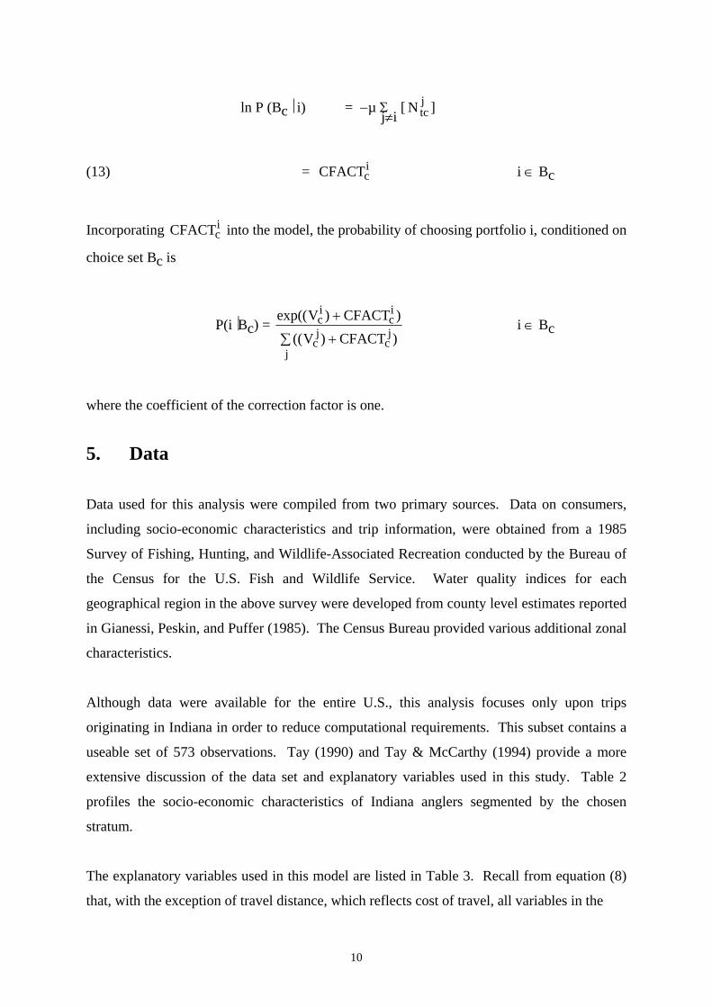
(13) = CFACT i Bc ci

Incorporating CFACT into the model, the probability of choosing portfolio i, conditioned on

choice set Bc is

ci

P(iBc) = exp(( ) )

(( ) )

V CFACT

V CFACTci

ci

cj

cj

j

i Bc

where the coefficient of the correction factor is one.

5. Data

Data used for this analysis were compiled from two primary sources. Data on consumers,

including socio-economic characteristics and trip information, were obtained from a 1985

Survey of Fishing, Hunting, and Wildlife-Associated Recreation conducted by the Bureau of

the Census for the U.S. Fish and Wildlife Service. Water quality indices for each

geographical region in the above survey were developed from county level estimates reported

in Gianessi, Peskin, and Puffer (1985). The Census Bureau provided various additional zonal

characteristics.

Although data were available for the entire U.S., this analysis focuses only upon trips

originating in Indiana in order to reduce computational requirements. This subset contains a

useable set of 573 observations. Tay (1990) and Tay & McCarthy (1994) provide a more

extensive discussion of the data set and explanatory variables used in this study. Table 2

profiles the socio-economic characteristics of Indiana anglers segmented by the chosen

stratum.

The explanatory variables used in this model are listed in Table 3. Recall from equation (8)

that, with the exception of travel distance, which reflects cost of travel, all variables in the

10

indirect utility function enter as a weighted sum where the weights are total times spent at

each site,

(14) Zk = r (TSr)(zr)

Because the portfolio choice set is unordered and consumer socio-economic characteristics

do not vary by portfolio, consumer attributes enter the model through interaction terms with

total recreational time. As seen in Table 3, the model interacts total recreational time with

four socio-economic variables: INC (a dummy variable which equals 1 for households with

incomes over $20,000 and 0 otherwise); OLDER (a dummy variable which equals 1 for

anglers at least 45 years of age and 0 otherwise); BASS (a dummy variable which equals 1

for a bass angler and 0 otherwise); and RIVER (a dummy variable which is one for moving

water and 0 otherwise).

Since recreation is a normal good, it is expected that the income interaction term will be

positive. Relative to households with incomes less than $20,000, an increase in total

recreation time will increase the probability of a portfolio's choice among higher income

households. Similarly, since older anglers may have more flexible time constraints, an

increase in total time spent fishing is expected to increase an older angler's portfolio demand

relative to that of a younger angler's demand.

Related to this, there may be a difference among anglers that fish for a particular species

relative to anglers with no specific preferences for type of fish caught. To test this

hypothesis, BASS was interacted with total recreation time. A positive sign on this

coefficient would indicate that, relative to anglers with non-specific preferences, an increase

in the total time spent fishing will increase a bass fishermen's portfolio demand. Last,

RIVER is included to differentiate moving water from enclosed water sources which offer

differing fishing opportunities and other amenities. A priori, the effect on portfolio demand

from an increase in recreational time spent river fishing, relative to fishing in enclosed sites,

is ambiguous.

As discussed above, an increase in the distance travelled increases the cost of accessing the

site and, all else constant, is expected to decrease the demand for recreational fishing.

Because cost information, either generally or by alternative modes, was not available, total

11

distance between an angler's origin zone and each of the destination zones in the portfolio,

weighted by the number of trips (see equation (8)), was used to reflect the cost of a portfolio.

However, this may lead to a selection bias since an angler's total trip distance may depend

upon the portfolio chosen. In order to control for a potential endogeneity bias, total trip

distance was regressed on several exogenous variables (number of trips, duration of trips,

income, total suspended solids and faecal coliform bacteria) and predicted trip distance,

rather than actual trip distance, was included in the portfolio choice model. The results were,

in general, quite robust to instrumenting out distance.

A zone's water quality is assumed to be an important consideration in one's selection of a

fishing site. From equation (14), the total time spent in region r, weighted by indices of a

region's water quality, was interpreted as an index of a portfolio's water quality. In this paper,

two widely used measures of water quality (Train, 1979), Faecal Coliform Bacteria (FCB)

and Total Suspended Solids (TSS), that have negative health and visual effects, are used to

form portfolio water quality indices. Since an increase in the concentration of each of these

is expected to reduce a region's attractiveness, it is expected that each coefficient will have a

negative sign.

The destinations used in the survey and the created portfolios are not specific sites, such as a

particular lake or stretch of river, but rather large geographical areas which embody a number

of angling opportunities. Because the size of an aggregate alternative influences an

individual's choice (Ben-Akiva and Lerman (1985)), we interact recreation time with the total

water surface area (TWA) to capture the differences in a region's size and angling

opportunities.

In addition to differences in sizes, there are likely to be differences among regions along

dimensions that are not explicitly captured by the socio-economic and water quality

interactions. In order to capture nonsize related heterogeneity of the region, we interact

total recreation time with two additional regional characteristics, the proportion of a region's

land area used in farming (FARM) and the total wooded area (WOOD). All else constant, an

increase in either amenity, as compared to more developed areas, is expected to increase an

angler's portfolio demand.

12

Finally, the coefficient of the sampling correction factor, CFACT, is constrained to one.

When the constraint was removed, however, the coefficient was not significantly different

from 0 but estimates for the other variables remained relatively stable.

6. Estimation Results

Table 4 presents the estimation results. In general, the model fits well with a highly

significant 2. All coefficients have their anticipated signs and most are highly significant.

As expected, increases in the total cost of a portfolio, measured as the total distance an angler

travels to reach one's destinations in a given portfolio, reduced the portfolio's demand, all else

held constant. Also, a logarithmic specification for total distance provided the best fit of the

model indicating that an increase in a portfolio's distance decreases indirect utility but at a

decreasing rate.

The positive influence of income on recreational fishing is consistent with expectations,

indicating that an increase in a portfolio's recreational time increases the portfolio's demand

among higher income households relative to lower income households. Alternatively,

holding total time constant, a portfolio's demand increases with income indicating that fishing

is a normal good, as expected.

Also consistent with expectations, an increase in total angling time increased portfolio

demands among older anglers relative to their younger counterparts. This is consistent with

the hypothesis that time constraints among older anglers are less binding and result in a

higher demand for fishing, all else constant.

Increasing angling time increases portfolio demands among bass fishermen, suggesting that

bass fishermen place higher values upon angling opportunities than general fishermen, a

result that is consistent with other studies (Parsons and Needelman, 1992). And relative to

fishing in enclosed waters, increases in total recreation time increased the portfolio demands

of river anglers. All else constant, the results reveal a larger demand for river fishing than

fishing in lakes or other enclosed sites.

13

As expected, an increase in total water surface increases the probability of choosing that

portfolio, all else constant. Although it may be interpreted as a 'size' measure of the available

alternatives, the logarithm of total water surface is not the same as the number of elemental

alternatives in a portfolio because the number of elemental alternatives is not well-defined in

a portfolio. Thus, total water surface is used in the model to capture differences in the

attractiveness of portfolios due to destinations of varying sizes included in one's portfolio. It

might be noted, however, that the estimated coefficient lies between zero and one which is

consistent with random utility maximization when the variable is included as a measure of

size (Ben-Akiva and Lerman, 1985). Related to this, both the total wooded area and the

proportion of the zone used as farmland are strongly significant with their expected signs,

consistent with the hypothesis that each variable is capturing regional heterogeneity

We argued earlier that water quality considerations are an important input into an angler's

portfolio demands and the results presented in Table 4 bear this out. Holding all else

constant, pollution increases in the form of fetal coliform bacteria and total suspended solids

reduce portfolio demands.

7. Choice Elasticities

In addition to the elasticity of the choice probabilities with respect to distance, elasticities

with respect to the water qualities provide useful information on consumers' responsiveness

to changes in these variables. This is of particular importance since the water quality of our

environment has become a concern of many government, private organisation and consumers

in recent years.

Although consistent parameter estimates can be obtained using a subset, Bc, of the

alternatives, elasticities are computed over the entire choice set,c. Given the large number

of portfolios available to consumers, it is infeasible to enumerate over the universal set.

Instead, Atherton et al. (1990) suggested using consistent estimates of the choice probabilities

and unbiased estimates of the variables for which the elasticities are measured. These

estimators are defined as

14

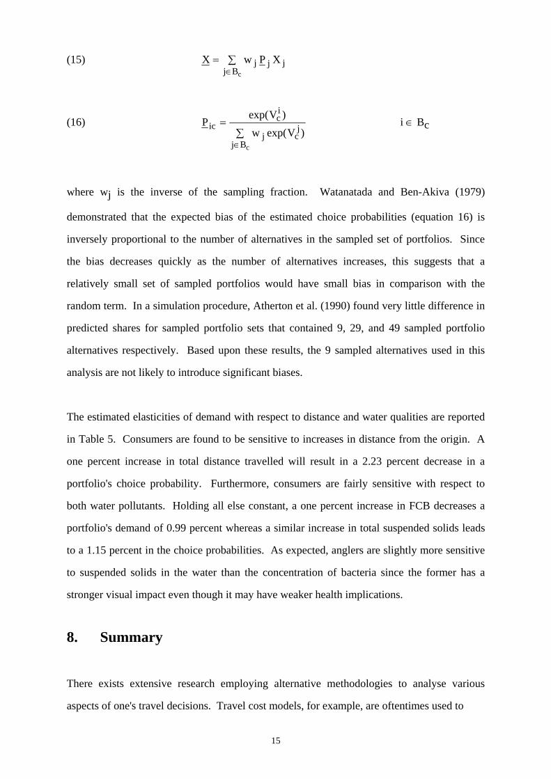
(15) X w Pj j jj Bc

X

(16) PV

w Vic

ci

j cj

j Bc

exp( )

exp( ) i Bc

where wj is the inverse of the sampling fraction. Watanatada and Ben-Akiva (1979)

demonstrated that the expected bias of the estimated choice probabilities (equation 16) is

inversely proportional to the number of alternatives in the sampled set of portfolios. Since

the bias decreases quickly as the number of alternatives increases, this suggests that a

relatively small set of sampled portfolios would have small bias in comparison with the

random term. In a simulation procedure, Atherton et al. (1990) found very little difference in

predicted shares for sampled portfolio sets that contained 9, 29, and 49 sampled portfolio

alternatives respectively. Based upon these results, the 9 sampled alternatives used in this

analysis are not likely to introduce significant biases.

The estimated elasticities of demand with respect to distance and water qualities are reported

in Table 5. Consumers are found to be sensitive to increases in distance from the origin. A

one percent increase in total distance travelled will result in a 2.23 percent decrease in a

portfolio's choice probability. Furthermore, consumers are fairly sensitive with respect to

both water pollutants. Holding all else constant, a one percent increase in FCB decreases a

portfolio's demand of 0.99 percent whereas a similar increase in total suspended solids leads

to a 1.15 percent in the choice probabilities. As expected, anglers are slightly more sensitive

to suspended solids in the water than the concentration of bacteria since the former has a

stronger visual impact even though it may have weaker health implications.

8. Summary

There exists extensive research employing alternative methodologies to analyse various

aspects of one's travel decisions. Travel cost models, for example, are oftentimes used to

15

model trip frequencies whereas multinomial logit models are typically employed to analyse

destination choices. However, these models are limited by their narrow focus upon a single

aspect of travel. Recreational decisions reflect a complex decision-making process which

encompasses a set of interrelated decisions, including choice of frequency, duration, and

destination. In the recent past, more general models, based upon discrete choice frameworks,

of travel-related demands have been developed in order to explicitly account for the

interrelated nature of recreational demands.

One class of models is a nested logit framework which incorporates sequential choice

decisions while another approach models these decisions simultaneously using joint logit

analysis (Hensher and Johnson, 1981; Ben-Akiva and Lerman, 1985; and Train, 1987).

These models, however, are essentially 'single destination - single duration - single frequency'

choice models.

An alternative approach presented here is to model the full set of recreational demands per

time period. Relative to this context, previous research that modelled multi-dimensional

travel choices has captured only one element in a consumer's annual portfolio, that is, a single

Nrd is modelled. All non-zero elements in a consumer's portfolio are included as repeated

observations or one element is randomly sampled and others are discarded.

In general, the results of this research conform to expectations. Increases in the attractiveness

of a given recreational fishing portfolio, all else constant, increase the probability of that

portfolio being chosen. Improvements in a portfolio's overall water quality and aesthetic

characteristics (reflected by the extent of a region that is wooded, for example) were found to

increase the probability that the portfolio was selected. And increases in the expected costs

associated with a portfolio's destinations were found to decrease the probability of choosing

that portfolio, as expected. Generally consistent with other studies, portfolio choice

elasticities with respect to water quality were found to be in the unitary elasticity range.

Furthermore, portfolio recreational demands were sensitive to distance travelled. A one

16

percent increase in a portfolio's distance is associated with a 2.23 percent decrease in the

portfolio's demand.

A portfolio approach to recreational demands facilitates the modeling of multidimensional

decision processes and avoids the accounting problem involved with the timing of trip

decisions. However, this approach is also restrictive since it assumes that, at the beginning of

the period, consumers decide upon their recreational travel packages for the entire period.

Also, unless all of a consumer's recreational choices involve fishing, the approach in this

paper ignores the impact that recreational fishing decisions have upon other recreational

choices.

These limitations suggest areas for further research. Included among these would be a

comparative analysis of the implications of a portfolio approach with nested logit type

structures that concentrate on one multidimensional decision to the exclusion of others that

are made in the same time period. Second, do consumers easily substitute recreational

fishing for other recreational activities or is it appropriate to view a consumer's decision as a

two stage budgeting process wherein a consumer first decides upon a recreational budget and

then allocates that budget to alternative recreational activities?

17

References

Adler T. and Ben-Akiva M. (1979). Joint choice model for frequency, destination, and

travel mode for shopping trips. Transportation Research Record, 569, 136-150. Atherton et al. (1990). Micro-simulation of local residential telephone demand under

alternative service options and rate structures. In Fontenay et al. (eds.), Telecommunications Demand Modeling: An Integrated View. New York: North Holland.

Ben-Akiva M. and Lerman S. (1985). Discrete Choice Analysis: Theory and Application to

Travel Demand. Cambridge: MIT Press. Bockstael et al. (1984). Measuring the benefits of water quality improvements using

recreation demand models. Volume II of Benefit analysis using indirect or imputed market methods. Department of Agricultural and Resource Economics, University of Maryland, College Park.

Brown H. (1979). A model of weekend recreational travel demand. Working paper

RP/06/79/Trans, Department of Civil Engineering, University of Melbourne, Australia. Reproduced in Hensher D. and Johnson L. (1981).

Caulkins et al. (1985). Travel cost model for lake recreation: A comparison of two methods

for incorporating site quality and substitution effects. American Journal of Agricultural Economics. 68, 291-297.

Gianessi et al. (1985). National data base of nonurban nonpoint source discharges and their

effect on the nation's water quality. Resources for the Future, Washington, D.C. Hensher D. and Johnson L. (1981). Applied Discrete Choice Modeling. London: Croom

Helm Ltd. Kealy M. and Bishop R. (1986). Theoretical and empirical specifications issues in travel

cost demand studies. American Journal of Agricultural Economics, 68, 660-67. McFadden D. (1978). Modeling residential choice location. In Karlqvist et al. (eds.),

Spatial Interaction Theory and Planning Models. Amsterdam: North Holland. Parsons G. and Needelman M. (1992). Site aggregation in a random utility model of

recreation. Land Economics, 68, 418-433. Ribaudo et al. (1984). Recreation benefits from an improvement in water quality at St.

Albans Bay, Vermont. Economic Research Service Staff Report No. AGES840127. Washington D.C.: U.S. Department of Agriculture.

Smith V. (1988). Selection and recreation demand. American Journal of Agricultural

Economics, 70, 29-36. Smith V. and Kaoru Y. (1986). Modeling recreation demand within a random utility

framework. Economic Letters, 22, 395-399.

18

19

Tay R. (1990). Modeling recreational activities using discrete choice frameworks. Ph.D.

Dissertation, Department of Economics, Purdue University. Tay R. and McCarthy P. (1994). Benefits of improved water Quality: A discrete choice

analysis of freshwater recreational demands. Environment and Planning, 26A, 1625-1638.

Train R. (1979). Quality Criteria for Water. London: Castle House Publications. Train, K. (1986). Qualitative Choice Analysis. Cambridge: MIT Press. Train et al. (1987). The demand for local telephone services: A fully discrete model of

residential calling patterns and service choices. Rand Journal of Economics, 18,109-23. U.S. Department of Commerce (1987a). Survey of fishing, hunting, and wildlife - associated

recreation, 1985. Washington D.C.: Bureau of the Census. U.S. Department of Commerce (1987b). Survey of fishing, hunting, and wildlife -

associated recreation. 1985 tape technical documentation, prepared by the Data User Services Division. Washington D.C.: Bureau of the Census.

Watanatada T. and Ben-Akiva M. (1979). Forecasting urban travel demand for quick policy

analysis with disaggregate choice models: A monte carlo simulation approach. Transportation Research, 13A, 241-248.

*

Table I Uisi rihution of Trips'"

One Day Two Day Three or l\'lore All Trips Trips Day Trips Trips

'Yo. "/" %. "/"

Onglll Zones 662X 474 I 79 72XI

Contiguous 1364 371 1.10 IX 45

Zones

Outer Zones 6.10 1.2X 1 36 X 74

. All Zones X602 973 4.25 100 (H)

For the contiguous zones and outer zones, the percentages have to be divided by two for each zone drawn.

20

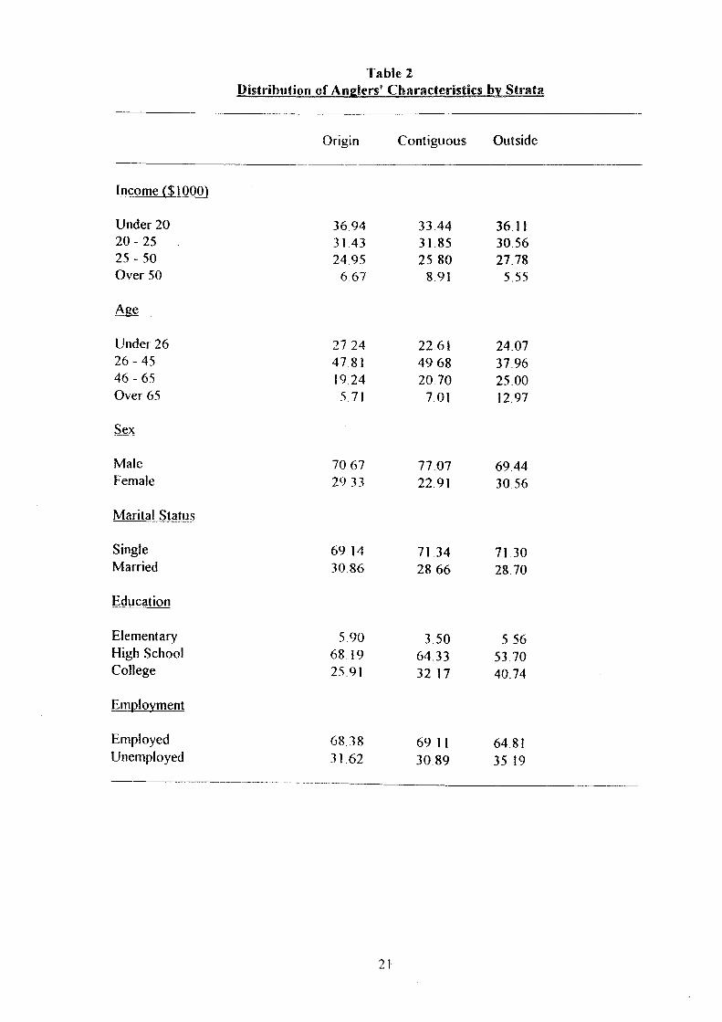
Table 2 Distribution of Ans:;lers' Characteristics by Strata

Origin Contiguous Outside

Income ($1000)

Under 20 36.94 33.44 36.11 20 - 25 3143 31.85 30.56 25 - 50 24.95 2580 27.78 Over 50 6.67 891 5.55

Age

Under 26 27 24 22.61 24.07 26 - 45 4781 4968 37.96 46 - 65 1924 20.70 25.00 Over 65 ).71 701 12.97

Sex

Male 7067 7707 69.44 Female 2933 22.91 3056

Marital Status

Single 6914 71.34 71.30 Married 30.86 28.66 28.70

Education

Elementary 590 3.50 5.56 High School 68.19 64.33 53.70 College 259) 3217 40.74

Employment

Employed 68.38 69.11 64.81 Unemployed 3162 30.89 35.19 -------_._-_ ... _---_ .... _ .. _- '- ---- ---_. __ .

21

Table 3 Description of Exphm~'tory Variables

Variables

(OLDER)( L TSr) r

(INC)( LTS r) r

(BASS)( L TS r) r

(RIVER)( L TSr) r

In I L (Nr)(DlST») r

In [ L (TSr)(TW A) I r

In [ L (TSr)(WOOD) J r

L (TSr)(F ARM) r

CFACT

Expected Sign

+

+

.~

+

+

+

22

Description of Variable

Total recreation time of anglers \\ho are 45 years or older.

Total recreation time of anglers with income over $20,000

T olal recreation time of bass anglers

Total recreational time of anglers \\ ho fish in fivers

Faecal Colifonn Bacteria (Illg/I)

Total Suspended Solids (Illg/I)

Logarithm of Distance Travelled (miles)

Logarithm of Total Water Area (sq. miles)

Logarilhm ofWc)()(kd Area ( sq miles)

Farm Area as a Percentage ofTolal Area

Samplll1g Correction Factor

Table 4 Estimation Results

Variables Coefficients T -Statistics

In I 1: (Nr)(DlST) I -2544 r

1: (TSr)(FCB) -2939 r

1: (TSr)(TSS) --02074 r

(BASS) (1: TCr) OOXOX r

(RIVER) ( L TS r) () 0597 r

(OLDER) ( L TS r) 00309 r

(INC) ( L TS r) o 04(j(j r

In I 1: (TSr)(TW A) I 02035 r

In I L (TSr)(WOOD) I 1372 r

1: (TSr)(FARM) 0797 r

~

Maximum Log Likelihood (P = f3 ) Restricted Log Likelihood (P = 0) Chi-Square ( df = X )

Number of Obsenations Number of Records Likelihood Ratio Index

-9.4

-9.4

-67

13.2

109

5.5

75

1.7

8.3

3.6

- 1160.96

-1319.38 318.76 57300

573000 0.1201

Attributes TSS

Elasticities I 1544

Table 5 Choice Elasticities

FCB

O.9X90

24

Travel Cost

2226