A population Monte Carlo scheme with transformed weights and its application to stochastic kinetic...

arX

iv:1

208.

5600

v1 [

stat

.CO

] 2

8 A

ug 2

012

Noname manuscript No.(will be inserted by the editor)

A population Monte Carlo scheme with transformed

weights and its application to stochastic kinetic models

Eugenia Koblents · Joaquın Mıguez

Received: date / Accepted: date

Abstract This paper addresses the problem of Monte Carlo approximation ofposterior probability distributions. In particular, we have considered a recentlyproposed technique known as population Monte Carlo (PMC), which is basedon an iterative importance sampling approach. An important drawback of thismethodology is the degeneracy of the importance weights when the dimensionof either the observations or the variables of interest is high. To alleviate thisdifficulty, we propose a novel method that performs a nonlinear transforma-tion on the importance weights. This operation reduces the weight variation,hence it avoids their degeneracy and increases the efficiency of the importancesampling scheme, specially when drawing from a proposal functions which arepoorly adapted to the true posterior.

For the sake of illustration, we have applied the proposed algorithm tothe estimation of the parameters of a Gaussian mixture model. This is a verysimple problem that enables us to clearly show and discuss the main featuresof the proposed technique. As a practical application, we have also consid-ered the popular (and challenging) problem of estimating the rate parametersof stochastic kinetic models (SKM). SKMs are highly multivariate systemsthat model molecular interactions in biological and chemical problems. Weintroduce a particularization of the proposed algorithm to SKMs and presentnumerical results.

Keywords Population Monte Carlo · importance sampling · degeneracy ofimportance weights · stochastic kinetic models

E. Koblents and J. MıguezDepartment of Signal Theory and Communications, Universidad Carlos III de Madrid,Madrid, SpainE-mail: ekoblents,[email protected]

http://arxiv.org/abs/1208.5600v1

2 Eugenia Koblents, Joaquın Mıguez

1 Introduction

The problem of performing inference in high dimensional spaces appears inmany practical applications. For example, it is of increasing interest in thebiological sciences to develop new techniques that allow for the efficient esti-mation of the parameters governing the behavior of complex autoregulatorynetworks. The main difficulty often encountered when tackling this kind ofproblems is the design of numerical inference algorithms which are stable andhave a guaranteed convergence also in high-dimensional spaces.

A very common strategy, which has been successfully applied in a broadvariety of complex problems, is the Monte Carlo methodology. In particu-lar, we have considered a recently proposed technique known as populationMonte Carlo (PMC) [7], which is based on an iterative importance samplingapproach. The aim of this method is the approximation of static probabilitydistributions by way of discrete random measures consisting of samples andassociated weights. The target distribution is often the posterior distributionof a set variables of interest, given some observed data.

The main advantages of the PMC scheme, compared to the widely estab-lished Markov chain Monte Carlo (MCMC) methodology, are the possibilityof developing parallel implementations, the sample independence and the factthat an unbiased estimate is provided at each iteration, which avoids the needof a convergence period.

On the contrary, an important drawback of the importance sampling ap-proach, and particulary of PMC, is that its performance heavily depends onthe choice of the proposal distribution (or importance function) that is usedto generate the samples and compute the weights. When the dimension of thevariables of interest is large, or the target probability density function (pdf)is very sharp with respect to the proposal (this occurs when, e.g., the num-ber of observations is high or when the prior distribution is uninformative),the importance weights degenerate1 leading to an extremely low number ofrepresentative samples. This problem is commonly known as weight degen-eracy and is closely related to the “curse of dimensionality”. To the best ofour knowledge, the degeneracy problem has not been successfully addressedso far in the PMC framework. The issue was already mentioned in the originalpaper [7], though, noting that the proposed scheme did not provide neither astabilization of the so called effective sample size, nor of the variance of theimportance weights.

The effort in the field of PMC algorithms has been mainly directed to-ward the design of efficient proposal functions. A recently proposed schemefor the proposal update is the mixture PMC technique [6], that models theimportance functions as mixtures of kernels. Both the weights and the inter-nal parameters of each mixture component are adapted along the iterationswith the goal of minimizing the Kullback-Leiber divergence between the target

1 In this context, degeneracy means that the vast majority of importance weights becomenegligible (practically zero) except for a very small number of them [10, 15].

Population Monte Carlo with transformed weights 3

density and the proposal. However, this scheme also suffers from degeneracyunless applied to very simple examples and the authors of [6] propose to ap-ply an additional Rao-Blackwellization scheme to mitigate the problems thatappear in multidimensional problems.

Another recently proposed PMC scheme [17] is based on the Gibbs sam-pling method and constructs the importance functions as alternating con-ditional densities. Thus, this method allows to sample efficiently from high-dimensional proposals. However, the importance weights still present severe de-generacy due to the extreme values of the likelihood function in high-dimensionalspaces, unless the number of samples is extremely high. The technique is basedon the multiple marginalized PMC, proposed in [4], [19].

In this paper we propose a novel PMC method, termed nonlinear PMC(NPMC). The emphasis is not placed on the proposal update scheme, whichcan be very simple (here we restrict ourselves to importance functions chosenas multivariate normal denisities whose parameters are adjusted along the it-erations to match the moments of the latest approximation of the posteriordistribution). The main feature of the technique is the application of a nonlin-ear transformation to the importance weights in order to reduce their varia-tions. In this way, the efficiency of the sampling scheme is improved (speciallywhen drawing from “poor” proposals) and, most importantly, the degeneracyof the weights is drastically mitigated even when the number of generated sam-ples is relatively small. We show analytically that the approximate integralscomputed using the transformed weights converge asymptotically to the trueintegrals.

In this work we have successfully applied the proposed methodology totwo different problems where severe weight degeneracy is observed. The firstexample is a Gaussian mixture model, already discussed in [7]. We have usedthis example to illustrate the degeneracy problem and for comparison of theoriginal PMC scheme with the proposed methods. We provide numerical re-sults that suggest that degeneracy of the importance weights takes places evenin simple and low-dimensional problems, when the proposal pdf is wide withrespect to the target. The proposed method clearly outperforms the originalPMC scheme and provides a high number of representative samples and veryaccurate estimates of the variables of interest.

As a practical application, we have also applied the proposed algorithm tothe popular (and challenging) problem of estimating the rate parameters instochastic kinetic models [3]. Such models describe the time evolution of thepopulation of a set of species or chemical reactions, which evolve accordingto a set of constant rate parameters, and present an autoregulatory behavior.This problem is currently of great interest in a broad diversity of biologicaland molecular problems, such as complex auto-regulatory gene networks.

We introduce a particularization of the generic NPMC algorithm to SKMs,which tackles the evaluation of the likelihood function (which can not be com-puted exactly) using a particle filter. As a simple and intuitive, yet physi-cally meaningful example, we have obtained numerical results for the Lotka-Volterra model, also known as predator-prey model, consisting of two inter-


acting species related by three reactions with associated unknown rates. Theproposed method provides a very good performance also in this scenario, wherestandard PMC algorithms can be easily shown to fail.

The rest of the paper is organized as follows. In Section 2 we introduce somenotation. In Section 3, we give a formal statement of the class of problems ad-dressed in this paper. In Section 4, the population Monte Carlo algorithm ispresented and a discussion of the weight degeneracy problem is provided. Insection 5 the proposed algorithm is described. In section 6 we provide a theo-retical convergence analysis of the new methodology. In section 7 we presentnumerical results on a Gaussian mixture model. We illustrate the effects ofdegeneracy and the performance of the proposed algorithms in this scenario.In Section 8, we describe the practical application of the proposed algorithmto the problem of estimating the constant rates of a stochastic kinetic model,and present numerical results. Section 9 is devoted to the conclusions.

2 Notation

In this section we introduce some notations that are used through the paper.

– All vectors are assumed to have column form. We denote them using bold-face lower-case letters, e.g., θ, y, and its k-th scalar component is written asthe corresponding normal-face letter with a subscript, e.g., θk, yk. Matricesare denoted by boldface upper-case letters, e.g., Σ. N .

– We use RK , with integerK ≥ 1, to denote the set of K-dimensional vectorswith real entries.

– B(RK) is the set of bounded real functions over RK . In particular, the

supremum norm of a real function f : RK → R is denoted as ‖f‖∞ =sup

z∈RK |f(z)| and f ∈ B(RK) when ‖f‖∞ < ∞.– The target pdf of a PMC algorithm is denoted as π, the proposal density

as q and the rest of pdf’s as p.– Wewrite conditional pdf’s as p(y|θ), and joint densities as p(θ) = p(θ1, . . . , θK).

This is an argument-wise notation, hence p(θ1) denotes the distribution ofθ1, possibly different from p(θ2), which represents the distribution of θ2.

– The integral of a function f with respect to a measure µ is denoted bythe shorthand (f, µ) =

∫

f(θ)µ(dθ). If the measure has a density π, i.e.,µ(dθ) = π(θ)dθ, then we also write (f, π) =

∫

f(θ)π(θ)dθ.– Ep(θ)[f(θ)] denotes expectation of the function f with respect to the prob-

ability distribution with density p(θ).

– A sample from the distribution of the random vector θ is denoted by θ(i).Sets of M samples {θ(1), . . . , θ(M)} are denoted as {θ(i)}Mi=1.

– δθ(i)(dθ) is the unit delta measure located at θ = θ(i).

– Unweighted samples are denoted with a tilde as{

θ(i)}

, opposite to the

corresponding weighted samples{

θ(i)}

.

– For a random value X , P{X < a} denotes the probability of the eventX < a.


– In the chemical representation the notation αx must not be interpreted asa product, but rather is read as “α molecules of species x”.

3 Problem Statement

Let θ = [θ1, . . . , θK ]⊤ be a vector of K unobserved real random variables with

prior density p(θ) and let y = [y1, . . . , yN ]⊤ be a vector of N real randomobservations related to θ by way of a conditional pdf p(y|θ).

In this paper we address the problem of approximating the posterior prob-ability distribution of θ, i.e., the distribution with density p(θ|y), using a ran-

dom grid ofM points, {θ(i)}Mi=1, in the space of the random vector θ. Once thegrid is generated, it is simple to approximate any moments of p(θ|y). For ex-ample, the posterior mean of θ given the observations y may be approximatedas

Ep(θ|y)[θ] =

∫

θp(θ|y)dθ ≈1

M

M∑

i=1

θ(i).

Unfortunately, the generation of useful samples that represent the proba-bility measure p(θ|y)dθ adequately when K (or N) is large is normally a verydifficult task. The main goal of this work is to devise and assess an efficientcomputational inference (Monte Carlo) methodology for the approximation ofp(θ|y)dθ and its moments, i.e., expectations of the form Ep(θ|y)[f(θ|y)], wheref : RK → R is some integrable function of θ.

4 Population Monte Carlo

4.1 Importance Sampling

One of the main applications of statistical Monte Carlo methods is the ap-proximation of integrals of the form

(f, π) =

∫

f(θ)π(θ)dθ,

where f is a real, integrable function of θ and π(θ) is some pdf of interest

(often termed the target density). Given the random sample{

θ(i)}M

i=1we

build a random discrete measure

πM (dθ) =1

M

M∑

i=1

δθ(i)(dθ)

that enables a straightforward approximation (f, πM ) of (f, π), namely

(f, π) ≈ (f, πM ) =

∫

f(θ)πM (dθ) =1

M

M∑

i=1

f(

θ(i))

.


Under mild assumptions, it can be shown that [18]

limM→∞

(f, πM ) = (f, π) a.s.

However, in many practical cases it is not possible to sample from π(θ)directly. A common approach to overcome this difficulty is to apply an im-portance sampling (IS) procedure [18]. The key idea is to draw the samples

{θ(i)}Mi=1 from a (simpler) proposal pdf, or importance function, q(θ), andthen compute associated importance weights of the form

w(i)∗ ∝π(

θ(i))

q(

θ(i)) ,

which we subsequently normalize to yield

w(i) =w(i)∗

∑M

j=1 w(j)∗

, i = 1, . . . ,M.

The integral (f, π) is then approximated by the weighted sum

(f, πM ) =

M∑

i=1

w(i)f(

θ(i))

.

The efficiency of an IS algorithm depends heavily on the choice of theproposal, q(θ). However, in order to ensure the asymptotic convergence of theapproximation (f, πM ), when M is large enough, it is sufficient to select q(θ)such that q(θ) > 0 whenever π(θ) > 0 [18].

Finally, note that the computation of the normalized weights requires thatboth π(θ) and q(θ) can be evaluated up to a proportionality constant inde-pendent of θ. This requirement is a mild one, since in most problems it ispossible to evaluate some function h(θ) ∝ π(θ).

4.2 Population Monte Carlo Algorithm

The population Monte Carlo (PMC) method [7] is an iterative IS schemethat seeks to generate a sequence of proposal pdf’s qℓ(θ), ℓ = 1, . . . , L, suchthat every new proposal is closer (in some adequate sense to be defined) tothe target density π(θ) than the previous importance function. Such schemedemands, therefore, the ability to learn about the target π(θ), given the setof samples and weights at the (ℓ − 1)-th iteration, in order to produce thenew proposal qℓ(θ) for the ℓ-th iteration. Taking this ability for granted, thealgorithm is simple and can be outlined as shown in Table 1.


Table 1 Generic PMC algorithm

Iteration (ℓ = 0, . . . , L):

1. Select a proposal pdf qℓ(θ).

– If π(θ) ∝ p(θ|y)p(θ), at iteration ℓ = 0 the proposal may be selected as the priorq0(θ) = p(θ).

– At iterations ℓ = 1, . . . , L, the proposal pdf qℓ(θ) must be adapted according to the

weighted sample{

θ(i)ℓ−1, w

(i)ℓ−1

}M

i=1at the previous iteration.

2. Draw a collection of M i.i.d. (independent and identically distributed) samples ΘMℓ

={

θ(i)ℓ

}M

i=1from qℓ(θ).

3. Compute the normalized weights

w(i)ℓ

∝π(

θ(i)ℓ

)

qℓ

(

θ(i)ℓ

) , i = 1, . . . ,M.

4. Perform a resampling step according to the weights w(i)ℓ

to create an unweighted sample

set ΘMℓ

={

θ(i)ℓ

}M

i=1.

At every iteration of the algorithm it is possible to compute, if needed, anestimate (f, πM

ℓ ) of (f, π) as

(f, πMℓ ) =

M∑

i=1

w(i)ℓ f

(

θ(i)ℓ

)

and, if the proposals qℓ(θ) are actually improved across iterations, then it canbe expected that the error

∣

∣(f, π)− (f, πMℓ )∣

∣ also decreases with ℓ.In problems of the type described in Section 3, the target density is the

posterior pdf of θ, i.e., π(θ) = p(θ|y) ∝ p(y|θ)p(θ), where p(y|θ) is the like-lihood function of the variable θ given the observations y. A straightforwardway of initializing the algorithm is to use the prior as the starting proposal,q0(θ) = p(θ).

A frequently used index for the performance of Monte Carlo samplingmethods is the effective sample size (ESS) M eff and its normalized version(NESS) Mneff , respectively defined as [18]

M eff =1

∑Mi=1

(

w(i))2 , and Mneff =

M eff

M.

These indices may be used to quantitatively monitor the convergence of thePMC algorithm and to stop the adaptation when the proposal has convergedto the target. Thus, ideally we expect to observe an increase in both measuresalong the iterations, withMneff approaching unity as the algorithm converges.

However, unless the proposal pdf is well tailored to the target density, theresulting importance weights will often present very large variations, leading


to a low number of effective samples. This problem is well known to affect ISschemes and is usually termed as the degeneracy of the weights [10, 15].

4.3 Degeneracy of the importance weights

The degeneracy of the importance weights is a problem that arises when thenormalized importance weights w(i), i = 1, ...,M , of a set of samples {θ(i)}Mi=1

present large fluctuations and the maximum of the weights, maxi w(i), is close

to one, leading to an extremely low number of representative samples (i.e.,samples with non negligible weights). This situation occurs when the targetand the proposal densities are approximately mutually singular, i.e., they have(essentially) have disjoint support. This problem has been addressed in the sce-nario of very large scale systems [2] and it has been proved that the maximumof the sample weights converges to one if the sample size M is sub-exponentialin the system dimension K.

The degeneracy of the weights as the dimension of the system increases isan intuitive fact and has been widely accepted as one of the main drawbacks ofIS schemes. Indeed, The degeneracy of the weights makes the application of ISto high dimensional systems (those with a large value of K) computationallyintractable. However, not only a large value of K leads to degeneracy. Indeed,it can be easily verified (numerically) that existing PMC methods can sufferfrom degeneracy even when applied to very simple (low dimensional) systems.Assume that the target pdf is the posterior, π(θ) ∝ p(θ|y)p(θ), and consider a

set of M samples {θ(i)}Mi=1 drawn from the prior pdf p(θ), which is the case atthe first iteration of the PMC algorithm. Assuming conditionally independentobservations, the importance weight associated to the i-th sample is given by

w(i) ∝ p(

y|θ(i))

=N∏

n=1

p(

yn|θ(i))

, i = 1, . . . ,M. (1)

Thus, the importance weights are obtained from a likelihood consisting of theproduct of a potentially large number of factors. This structure can lead tolarge fluctuations in the normalized importance weights and a very low numberof effective samples. In fact, the degeneracy problem was already identified inthe original work introducing the PMC methodology. The specific algorithmfor which simulations are displayed in [7] can be shown to present sharp vari-ations in the effective sample size and a large variance of the estimators aswell. However, to the best of our knowledge, no systematic solution has beenprovided so far for this problem.

A parallelism exists between high dimension and high number of observa-tions, both leading to computational problems. On one hand, as the dimensionK increases, clearly the chance to obtain a representative sample θ(i) decreases,since the state space is larger. On the other hand, as the number of observa-tions increases, the probability concentrates in a smaller region (the posteriorpdf is sharper as a consequence, e.g., of a structure such as in Eq. 1), whichagain leads to a low probability of obtaining representative samples.


Therefore, while the degeneracy of the weights increases critically withK [2], in low dimensinal systems it is mainly motivated by a high numberof observations N , unless the computational inference method is explicitlydesigned to account for this difficulty. In section 7 we present numerical re-sults to support this claim, which provides a rationale to understand the poorperformance of existing PMC algorithms in certain low dimensional models.

In this paper we introduce a new methodology to tackle the weight de-generacy problem, either due to large K or to large N . The key feature ofthe method is the application of a nonlinear transformation to the importanceweights, in order to reduce their variations and avoid degeneracy. As a result,we obtain a number of effective samples that is large enough to adequatelyperform the proposal update and provide consistent estimates of the variablesof interest. The new technique is introduced in Section 5 below.

5 Algorithms

In this section we describe the proposed algorithm, which is termed nonlinearPMC (NPMC). We adopt a very simple proposal update scheme, where theimportance functions are multivariate Gaussian pdf’s with moments matchedto our latest approximation of the posterior distribution. The key feature is theapplication of a nonlinear transformation of the importance weights. Besidesthe basic version of the algorithm, we propose an adaptive version where thistransformation is only applied when the value of the effective sample size isbelow a certain threshold. Finally, we explore different forms of the weighttransformation.

5.1 Nonlinear PMC

Assume, in the sequel, that the target pdf is the posterior density, i.e., π(θ) ∝p(θ|y)p(θ). For simplicity we select the importance functions in the PMCscheme as multivariate normal (MVN) densities. In the ℓ-th iteration

qℓ(θ) = N (θ;µℓ,Σℓ) , ℓ = 1, . . . , L,

where µℓ is the mean vector and Σℓ is a positive definite covariance marix.The parameters of the Gaussian proposal are chosen to match the moments ofthe distribution described by the discrete measure ontained after the (ℓ − 1)-th iteration of the PMC algorithm. In particular, we compute the mean andcovariance as

µℓ =1

M

M∑

i=1

θ(i)

ℓ−1 and (2)

Σℓ =1

M

M∑

i=1

(

θ(i)

ℓ−1 − µℓ

)(

θ(i)

ℓ−1 − µℓ

)⊤

. (3)


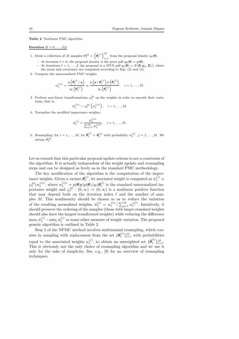
Table 2 Nonlinear PMC algorithm

Iteration (ℓ = 0, . . . , L):

1. Draw a collection of M samples ΘMℓ

={

θ(i)ℓ

}M

i=1from the proposal density qℓ(θ).

– At iteration ℓ = 0, the proposal density is the prior pdf q0(θ) = p(θ).– At iterations ℓ = 1, . . . , L the proposal is a MVN pdf qℓ(θ) = N (θ;µℓ,Σℓ), where

the mean and covariance are computed according to Eqs. (2) and (3).

2. Compute the unnormalized PMC weights

w(i)∗ℓ

=p(

θ(i)ℓ

| y)

qℓ

(

θ(i)ℓ

) ∝p(

y | θ(i)ℓ

)

p(

θ(i)ℓ

)

qℓ

(

θ(i)ℓ

) , i = 1, . . . ,M.

3. Perform non-linear transformations ϕMℓ

on the weights in order to smooth their varia-tions, that is,

w(i)∗ℓ

= ϕMℓ

(

w(i)∗ℓ

)

, i = 1, . . . ,M.

4. Normalize the modified importance weights,

w(i)ℓ

=w

(i)∗ℓ

∑Mj=1 w

(j)∗ℓ

, i = 1, . . . ,M.

5. Resampling: for i = 1, . . . ,M , let θ(i)ℓ = θ

(j)ℓ

with probability w(j)ℓ

, j = 1, . . . ,M . We

obtain ΘMℓ

.

Let us remark that this particular proposal update scheme is not a constraint ofthe algorithm. It is actually independent of the weight update and resamplingsteps and can be designed as freely as in the standard PMC methodology.

The key modification of the algorithm is the computation of the impor-

tance weights. Given a variate θ(i)ℓ , its asociated weight is computed as w

(i)ℓ ∝

ϕMℓ (w

(i)∗ℓ , where w

(i)∗ℓ = p(θ|y)p(θ)/qℓ(θ

(i)ℓ is the standard unnormalized im-

portance weight and ϕMℓ : (0,∞) → (0,∞) is a nonlinear positive function

that may depend both on the iteration index ℓ and the number of sam-ples M . This nonlinearity should be chosen so as to reduce the variation

of the resulting normalized weights, w(i)ℓ = w

(i)∗ℓ /

∑Mj=1 w

(j)∗ℓ . Intuitively, it

should preserve the ordering of the samples (those with larger standard weightsshould also have the largest transformed weights) while reducing the difference

maxi w(i)ℓ −mini w

(i)ℓ or some other measure of weight variation. The proposed

generic algorithm is outlined in Table 2.

Step 5 of the NPMC method involves multinomial resampling, which con-

sists in sampling with replacement from the set {θ(i)ℓ }Mi=1 with probabilities

equal to the associated weights w(i)ℓ , to obtain an unweighted set {θ

(i)

ℓ }Mi=1.This is obviously not the only choice of resampling algorithm and we use itonly for the sake of simplicity. See, e.g., [9] for an overview of resamplingtechniques.


At each iteration ℓ = 0, . . . , L, we obtain random discrete approximationsof the posterior distribution with density π(θ). Indeed, the discrete measures

πMℓ (dθ) =

M∑

i=1

w(i)ℓ δ

θ(i)ℓ

(dθ), and

πMℓ (dθ) =

1

M

M∑

i=1

δθ(i)ℓ

(dθ) (4)

are, both of them, approximations of π(θ)dθ. In particular, if f : RK → R isan arbitrary integrable function of θ, then the integral (f, π) =

∫

f(θ)π(θ)dθcan be approximated as either

(f, π) ≈ (f, πMℓ ) =

M∑

i=1

f(θ(i)ℓ )w

(i)ℓ or

(f, π) ≈ (f, πMℓ ) =

1

M

M∑

i=1

f(θ(i)ℓ ).

Note that the estimator (f, πMℓ ) involves one extra Monte Carlo step (be-

cause of resampling) and, hence, it can be shown to have more variance than(f, πM

ℓ ) [9]. Therefore, we assume in the sequel that estimates are computedby way of the measure πM

ℓ unless explicitly stated otherwise.Note as well that, since π(θ) ∝ p(θ|y)p(θ), any expectation with respect to

the posterior distribution is actually an integral with respect to the measureπ(θ)dθ, i.e., Ep(θ|y[f(θ)] = (f, π), and, therefore, it can be approximated usingπMℓ , namely, Ep(θ|y[f(θ)] = (f, πM

ℓ ).

5.2 Modified NPMC

The nonlinear transformation ϕMℓ is mainly useful at the first iterations of

the PMC scheme, when the proposal density does not fit the target densityand the standard importance weights may display high variability. However, insome applications it may be possible to remove the nonlinear transformationafter a few iterations, when the proposal is closer to the target.

Table 3 displays a modification of the NPMC algorithm which consistsin applying the nonlinear transformation only if the ESS is below a specifiedthreshold. The modified algorithm only differs in steps 3 and 4 from the genericNPMC procedure, and they are outlined in the table.

5.3 Selecting the transformation of the importance weights

Several possibilities exist for the choice of the nonlinearity ϕMℓ . In this section

we describe and intuitively justify two specific functions based on the “tem-pering” and the “clipping”, respectively, of the standard importance weights.


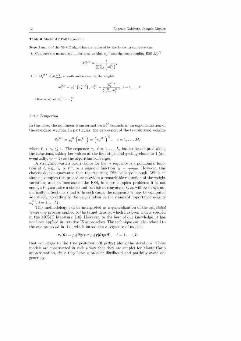
Table 3 Modified NPMC algorithm

Steps 3 and 4 of the NPMC algorithm are replaced by the following computations:

3. Compute the normalized importance weights w(i)ℓ

and the corresponding ESS Meffℓ

Meff

ℓ=

1∑M

i=1

(

w(i)ℓ

)2.

4. If Meff

ℓ< Meff

min, smooth and normalize the weights

w(i)∗ℓ

= ϕMℓ

(

w(i)∗ℓ

)

, w(i)ℓ

=w

(i)∗ℓ

∑Mj=1 w

(j)∗ℓ

, i = 1, . . . ,M.

Otherwise, set w(i)ℓ

= w(i)ℓ

.

5.3.1 Tempering

In this case, the nonlinear transformation ϕMℓ consists in an exponentiation of

the standard weights. In particular, the expression of the transformed weights

w(i)∗ℓ = ϕM

ℓ

(

w(i)∗ℓ

)

=(

w(i)∗ℓ

)γℓ

, i = 1, . . . ,M,

where 0 < γℓ ≤ 1. The sequence γℓ, ℓ = 1, . . . , L, has to be adapted alongthe iterations, taking low values at the first steps and getting closer to 1 (an,eventually, γℓ = 1) as the algorithm converges.

A straightforward a priori choice for the γℓ sequence is a polinomial func-tion of ℓ, e.g., γℓ ∝ ℓm, or a sigmoid function γℓ = 1

1−e−ℓ . However, thischoices do not guarantee that the resulting ESS be large enough. While insimple examples this procedure provides a remarkable reduction of the weightvariations and an increase of the ESS, in more complex problems it is notenough to guarantee a stable and consistent convergence, as will be shown nu-merically in Sections 7 and 8. In such cases, the sequence γℓ may be computedadaptively, according to the values taken by the standard importance weights

w(i)ℓ , i = 1, ...,M .This methodology can be interpreted as a generalization of the simulated

tempering process applied to the target density, which has been widely studiedin the MCMC literature, [18]. However, to the best of our knowledge, it hasnot been applied in iterative IS approaches. The technique can also related tothe one proposed in [14], which introduces a sequence of models

πℓ(θ) = pℓ(θ|y) ∝ pℓ(y|θ)p(θ), ℓ = 1, . . . , L

that converges to the true posterior pdf p(θ|y) along the iterations. Thesemodels are constructed in such a way that they are simpler for Monte Carloapproximation, since they have a broader likelihood and partially avoid de-generacy.


5.3.2 Clipping

In problems where the degeneracy of the weights is severe it is often difficult toapply a tempering procedure to soften the weights and to obtain a reasonableESS. The softening factor must take extremely low values at the first iterationsand a prior selection of the sequence γℓ is not straightforward.

In this work we propose a simple technique that consists in clipping thestandard weights that are above a certain threshold. As a consequence, asufficient number of “flat” (modified) weights is guaranteed in the regions ofthe space of theta where the standard weights were larger. The ESS becomescorrespondingly larger as well.

Specifically, the modified weights at iteration ℓ are computed from theoriginal importance weights as

w(i)∗ℓ = min

(

w(i)∗ℓ , T M

ℓ

)

, i = 1, . . . ,M,

where the threshold T Mℓ is selected to guarantee that the number of samples

θ(i)ℓ that satisfy w

(i)∗ℓ ≥ T M

ℓ is equal to MT < M . The parameter MT mustbe selected to represent adequately the multidimensional target posterior pdfπ(θ) = p (θ|y).

An alternative approach to the hard clipping technique described above, isto apply a sigmoid transformation to the standard weights, resulting in a softclipping, namely

w(i)∗

ℓ =2βℓ

1 + exp

(

−2w

(i)∗ℓ

βℓ

) − βℓ, i = 1, . . . ,M,

where βℓ > 0 should increase along the iterations in order to progressivelyreduce the nonlinear distortion of the standard weights.

6 Convergence of nonlinear importance sampling

The convergence of the original PMC scheme is easily justified by the conver-gence of the standard IS method. Indeed, it can be proved that the discrete

measure πMℓ (dθ) =

∑Mi=1 w

(i)ℓ δ

θ(i)ℓ

(dθ) converges to π(θ)dθ under mild as-

sumptions, meaning that

limM→∞

|(f, πMℓ )− (f, π)| = 0 (5)

almost surely (a.s.) for every ℓ ∈ {1, ..., L} and any f ∈ B(RK).In this section we provide a result similar to Eq. (5) for the discrete measure

πMℓ generated by the NPMC algorithm using a class of clipping transforma-

tions. The analysis, therefore, is concerned with the asymptotic performanceof the approximation as the number of amples M grows, and not with theiteration of the algorithm, i.e., not with the convergence as ℓ increases. Hence,we shall drop the latter subscript for convenience in the sequel.


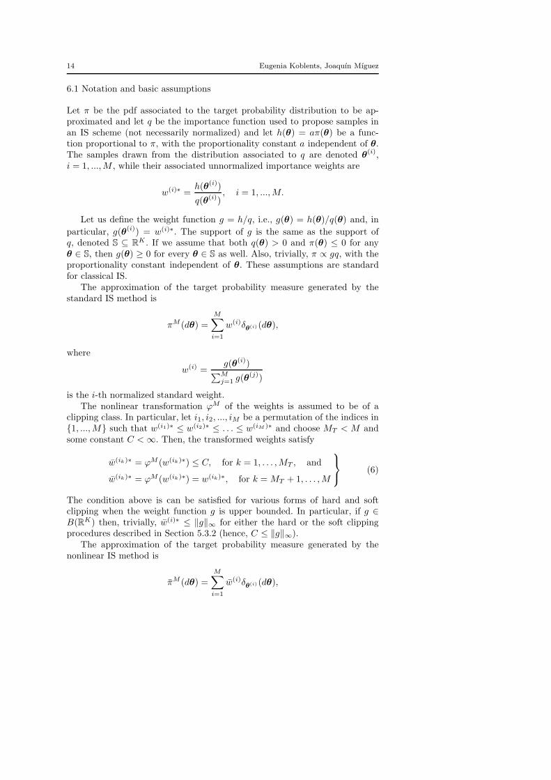
6.1 Notation and basic assumptions

Let π be the pdf associated to the target probability distribution to be ap-proximated and let q be the importance function used to propose samples inan IS scheme (not necessarily normalized) and let h(θ) = aπ(θ) be a func-tion proportional to π, with the proportionality constant a independent of θ.The samples drawn from the distribution associated to q are denoted θ(i),i = 1, ...,M , while their associated unnormalized importance weights are

w(i)∗ =h(θ(i))

q(θ(i)), i = 1, ...,M.

Let us define the weight function g = h/q, i.e., g(θ) = h(θ)/q(θ) and, in

particular, g(θ(i)) = w(i)∗. The support of g is the same as the support ofq, denoted S ⊆ R

K . If we assume that both q(θ) > 0 and π(θ) ≤ 0 for anyθ ∈ S, then g(θ) ≥ 0 for every θ ∈ S as well. Also, trivially, π ∝ gq, with theproportionality constant independent of θ. These assumptions are standardfor classical IS.

The approximation of the target probability measure generated by thestandard IS method is

πM (dθ) =

M∑

i=1

w(i)δθ(i)(dθ),

where

w(i) =g(θ(i))

∑Mj=1 g(θ

(j))

is the i-th normalized standard weight.The nonlinear transformation ϕM of the weights is assumed to be of a

clipping class. In particular, let i1, i2, ..., iM be a permutation of the indices in{1, ...,M} such that w(i1)∗ ≤ w(i2)∗ ≤ . . . ≤ w(iM )∗ and choose MT < M andsome constant C < ∞. Then, the transformed weights satisfy

w(ik)∗ = ϕM (w(ik)∗) ≤ C, for k = 1, . . . ,MT , and

w(ik)∗ = ϕM (w(ik)∗) = w(ik)∗, for k = MT + 1, . . . ,M

(6)

The condition above is can be satisfied for various forms of hard and softclipping when the weight function g is upper bounded. In particular, if g ∈B(RK) then, trivially, w(i)∗ ≤ ‖g‖∞ for either the hard or the soft clippingprocedures described in Section 5.3.2 (hence, C ≤ ‖g‖∞).

The approximation of the target probability measure generated by thenonlinear IS method is

πM (dθ) =M∑

i=1

w(i)δθ(i)(dθ),


where

w(i) =ϕM (g(θ(i)))

∑M

j=1 ϕ(g(θ(j)))

is the i-th normalized transformed weight. Additionally, we introduce a nonnormalized approximation of π(θ)dθ of the form

πM (dθ) =

M∑

i=1

w(i)δθ(i)(dθ), (7)

where

w(i) =ϕM (g(θ(i)))∑M

j=1 g(θ(j))

, i = 1, ...,M,

are non normalized transformed weights that will be referred to as “bridgeweights” in the sequel.

6.2 Asymptotic convergence

We aim at proving that limM→∞ |(f, πM )−(f, π)| = 0 a.s. for any f ∈ B(RK).To obtain such a result, we split the problem into simpler questions by applyingthe triangle inequality

|(f, πM )− (f, π)| ≤ |(f, πM )− (f, πM )|+ |(f, πM )− (f, π)|. (8)

The second term on the right hand side of (8) is handled easily using standardIS theory. For the first term, we have to prove that the discrete measuregenerated by the nonlinear IS method (πM ) converges to the discrete measuregenerated by the standard IS method (πM ). This can be done by resorting toanother triangle inequality,

|(f, πM )− (f, πM )| ≤ |(f, πM )− (f, πM )|+ |(f, πM )− (f, πM )|, (9)

that reveals the role of the bridge measure defined in (7).The following lemma establishes the asymptotic convergence of the term

|(f, πM )− (f, πM )| in inequality (9).

Lemma 1 Assume that limM→∞MT

M= 0, g ∈ B(RK), g > 0 and the trans-

formation function ϕM satisfies (6). Then, for every f ∈ B(RK) and suffi-ciently large M , there exist positive constants c1, c

′1 independent of M and MT

such that

P

{

∣

∣(f, πM )− (f, πM )∣

∣ ≤ c1MT

M

}

≥ 1− exp (−c′1M).

Proof: See Appendix A.Next, we establish the convergence of the bridge measure πM toward πM .


Lemma 2 Assume that g ∈ B(RK), g > 0 and the transformation functionϕM satisfies (6). Then, for every f ∈ B(RK) there exist positive constantsc2, c

′2 independent of M and MT such that

P

{

∣

∣(f, πM )− (f, πM )∣

∣ ≤ c2MT

M

}

≥ 1− exp (−c′2M).

Proof: See Appendix B.

The combination of Lemmas 1 and 2, together with the triangle inequality(9), yields the convergence of the error |(f, πM )− (f, πM )|.

Lemma 3 Assume that limM→∞MT

M= 0, g ∈ B(RK), g > 0 and the trans-

formation function ϕM satisfies (6). Then, for every f ∈ B(RK), and suffi-ciently large M , there exist positive constants c, c′ independent of M and MT

such that

P

{

∣

∣(f, πM )− (f, πM )∣

∣ ≤ cMT

M

}

≥ 1− 2 exp (−c′M).

In particular,

limM→∞

|(f, πM )− (f, πM )| = 0 a.s.

Proof: See Appendix C.

Finally, Lemma 3 can be combined with inequality (8) to yield the desiredresult, stated below.

Theorem 1 Assume that g ∈ B(RK) and the transformation function ϕM

satisfies (6) with C ≤ ‖g‖∞ independent of M . If limM→∞MT

M= 0 then, for

every f ∈ B(RK),

limM→∞

|(f, πM )− (f, π)| = 0 a.s.

Proof: It is classical result that

limM→∞

|(f, πM )− (f, π)| = 0 a.s. (10)

Combining (10) with the second part of Lemma 3 and the triangle inequalityin (8) yields the desired result. ⊓⊔

7 Example 1: a Gaussian mixture model

In this section we provide numerical results that illustrate the degeneracyproblem and the performance of the proposed NPMC scheme applied to theGaussian mixture model example of [7].


7.1 Problem setup

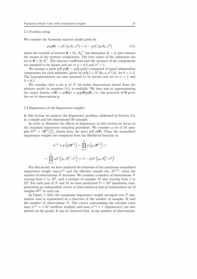
We consider the Gaussian mixture model given by

p(y|θ) = ρN(

y; θ1, σ2)

+ (1− ρ)N(

y; θ2, σ2)

(11)

where the variable of interest θ = [θ1, θ2]⊤ has dimension K = 2, and contains

the means of the mixture components. The true values of the unknowns areset to θ = [0, 2]⊤. The mixture coefficient and the variance of the componentsare assumed to be known and set to ρ = 0.2 and σ2 = 1.

We assume a prior pdf p(θ) = p(θ1)p(θ2) composed of equal independentcomponents for each unknown, given by p(θk) = N

(

θk; ν, σ2/λ)

, for k = 1, 2.The hyperparameters are also assumed to be known and set to ν = 1 andλ = 0.1.

We consider that a set y of N iid scalar observations drawn from themixture model in equation (11) is available. We thus aim at approximatingthe target density π(θ) = p(θ|y) ∝ p(y|θ)p(θ), i.e., the posterior of θ giventhe set of observations y.

7.2 Degeneracy of the Importance weights

In this section we analyze the degeneracy problem, addressed in Section 4.3,in a simple and low dimensional IS example.

In order to illustrate the effects of degeneracy, in this section we focus onthe standard importance sampling procedure. We consider a set of M sam-ples ΘM = {θ(i)}Mi=1 drawn form the prior pdf p(θ). Thus, the normalizedimportance weights are computed from the likelihood function as

w(i) ∝ p(

y|θ(i))

=

N∏

n=1

p(

yn|θ(i))

=

=

N∏

n=1

ρN(

yn; θ(i)1 , σ2

)

+ (1 − ρ)N(

yn; θ(i)2 , σ2

)

For this model, we have analyzed the behavior of the maximum normalizedimportance weight maxw(i) and the effective sample size M eff , when thenumber of observations N increases. We consider a number of observations Nvarying from 1 to 103, and a number of samples M also varying from 1 to103. For each pair of N and M we have performed P = 103 simulation runs,generating an independent vector of observations y and an independent set ofsamples ΘM in each run.

In Figure 1 (left) the maximum importance weight averaged over P sim-ulation runs is represented as a function of the number of samples M andthe number of observations N . The curves representing the extreme casesmaxiw

(i) = 1/M (uniform weights) and maxiw(i) = 1 (degeneracy) are also

plotted on the graph. It can be observed that, as the number of observations,


100

101

102

103

0

0.1

0.2

0.3

0.4

0.5

0.6

0.7

0.8

0.9

1

M

max

(wi )

11/MN=1N=10

N=102

N=103

100

101

102

103

100

101

102

103

M

mea

n E

SS

1MN=1N=10

N=102

N=103

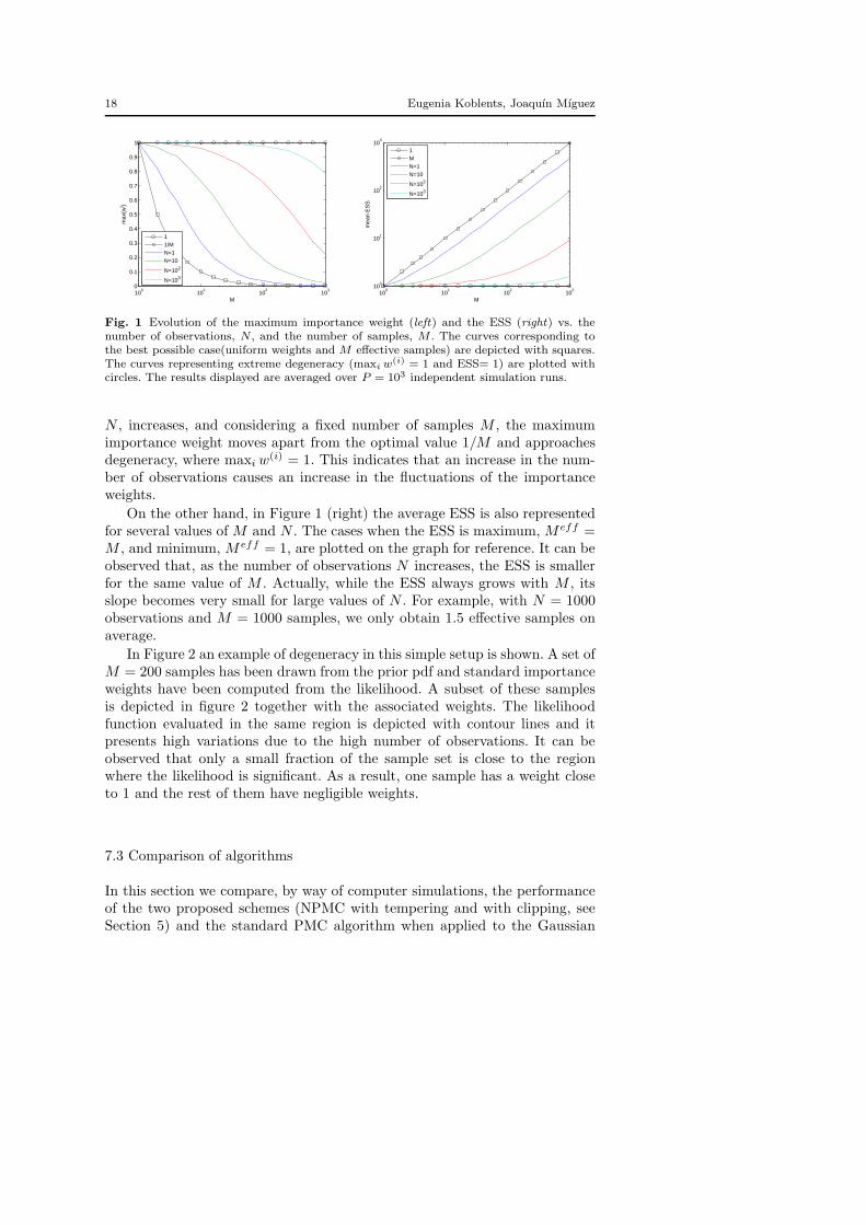
Fig. 1 Evolution of the maximum importance weight (left) and the ESS (right) vs. thenumber of observations, N , and the number of samples, M . The curves corresponding tothe best possible case(uniform weights and M effective samples) are depicted with squares.The curves representing extreme degeneracy (maxi w

(i) = 1 and ESS= 1) are plotted withcircles. The results displayed are averaged over P = 103 independent simulation runs.

N , increases, and considering a fixed number of samples M , the maximumimportance weight moves apart from the optimal value 1/M and approachesdegeneracy, where maxi w

(i) = 1. This indicates that an increase in the num-ber of observations causes an increase in the fluctuations of the importanceweights.

On the other hand, in Figure 1 (right) the average ESS is also representedfor several values of M and N . The cases when the ESS is maximum, M eff =M , and minimum, M eff = 1, are plotted on the graph for reference. It can beobserved that, as the number of observations N increases, the ESS is smallerfor the same value of M . Actually, while the ESS always grows with M , itsslope becomes very small for large values of N . For example, with N = 1000observations and M = 1000 samples, we only obtain 1.5 effective samples onaverage.

In Figure 2 an example of degeneracy in this simple setup is shown. A set ofM = 200 samples has been drawn from the prior pdf and standard importanceweights have been computed from the likelihood. A subset of these samplesis depicted in figure 2 together with the associated weights. The likelihoodfunction evaluated in the same region is depicted with contour lines and itpresents high variations due to the high number of observations. It can beobserved that only a small fraction of the sample set is close to the regionwhere the likelihood is significant. As a result, one sample has a weight closeto 1 and the rest of them have negligible weights.

7.3 Comparison of algorithms

In this section we compare, by way of computer simulations, the performanceof the two proposed schemes (NPMC with tempering and with clipping, seeSection 5) and the standard PMC algorithm when applied to the Gaussian


−2 −1 0 1 20

1

2

3

4

θ1

θ 2

5

10

15

20

25

30

35Samples θ(i)

θ(i), w(i)

p( y|θ1,θ

2)

Fig. 2 Subset of M = 200 samples θ(i) drawn form the prior p(θ) (blue circles) and theassociated standard importance weights (red circles with size proportional to the weightw(i)). The likelihood function p(y|θ) is depicted with contour lines.

Table 4 Standard PMC algorithm of [7].

Initialization (ℓ = 0):

1. Consider a set of p scales (variances) vj and an initial number rj = m of samples perscale, j = 1, . . . , p.

2. For i = 1, . . . ,M = pm, draw{

θ(i)0

}

from q0(θ) = p(θ).

Iteration (ℓ = 1, . . . , L):

1. For j = 1, . . . , p

– generate a sample{

θ(i)ℓ

}

of size rj from

qℓ (θ) = N(

θ(i)ℓ

;θ(i)ℓ−1, vjIK

)

, i = 1, . . . ,M,

– compute the normalized weights

w(i)ℓ

∝p(

y|θ(i)ℓ

)

p(

θ(i)ℓ

)

qℓ

(

θ(i)ℓ

) .

2. Resample with replacement the set{

θ(i)ℓ

}M

i=1according to the weights w

(i)ℓ

to obtain{

θ(i)ℓ

}M

i=1.

3. For j = 1, . . . , p update rj as the number of elements generated with variance vj whichhave been resampled.

mixture model. For convenience, we reproduce in Table 4 the original PMCscheme proposed in [7].

In order to asses the merit of an unweighted sample set {θ(i)k }Mi=1 for the

estimation of a scalar variable of interest θk, we evaluate the mean square error(MSE)

MSEk =1

M

M∑

i=1

(

θ(i)k − θk

)2

,


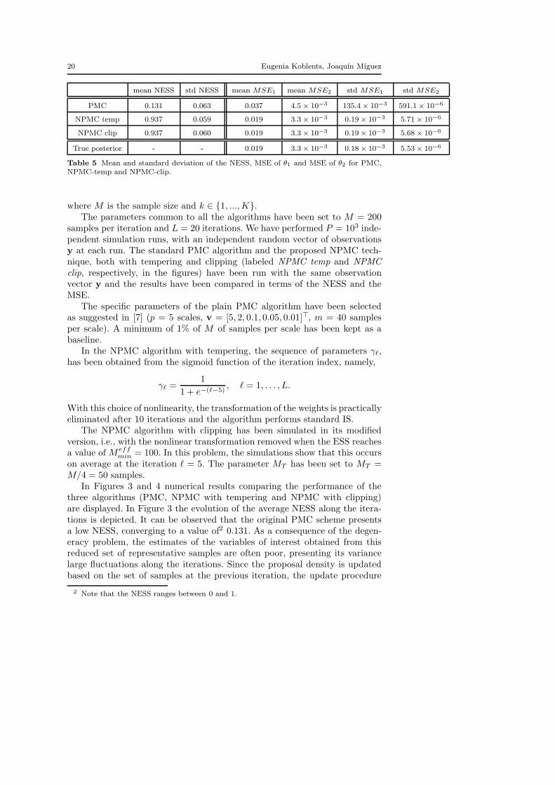
mean NESS std NESS mean MSE1 mean MSE2 std MSE1 std MSE2

PMC 0.131 0.063 0.037 4.5× 10−3 135.4× 10−3 591.1× 10−6

NPMC temp 0.937 0.059 0.019 3.3× 10−3 0.19× 10−3 5.71× 10−6

NPMC clip 0.937 0.060 0.019 3.3× 10−3 0.19× 10−3 5.68× 10−6

True posterior - - 0.019 3.3× 10−3 0.18× 10−3 5.53× 10−6

Table 5 Mean and standard deviation of the NESS, MSE of θ1 and MSE of θ2 for PMC,NPMC-temp and NPMC-clip.

where M is the sample size and k ∈ {1, ...,K}.The parameters common to all the algorithms have been set to M = 200

samples per iteration and L = 20 iterations. We have performed P = 103 inde-pendent simulation runs, with an independent random vector of observationsy at each run. The standard PMC algorithm and the proposed NPMC tech-nique, both with tempering and clipping (labeled NPMC temp and NPMCclip, respectively, in the figures) have been run with the same observationvector y and the results have been compared in terms of the NESS and theMSE.

The specific parameters of the plain PMC algorithm have been selectedas suggested in [7] (p = 5 scales, v = [5, 2, 0.1, 0.05, 0.01]⊤, m = 40 samplesper scale). A minimum of 1% of M of samples per scale has been kept as abaseline.

In the NPMC algorithm with tempering, the sequence of parameters γℓ,has been obtained from the sigmoid function of the iteration index, namely,

γℓ =1

1 + e−(ℓ−5), ℓ = 1, . . . , L.

With this choice of nonlinearity, the transformation of the weights is practicallyeliminated after 10 iterations and the algorithm performs standard IS.

The NPMC algorithm with clipping has been simulated in its modifiedversion, i.e., with the nonlinear transformation removed when the ESS reachesa value of M eff

min = 100. In this problem, the simulations show that this occurson average at the iteration ℓ = 5. The parameter MT has been set to MT =M/4 = 50 samples.

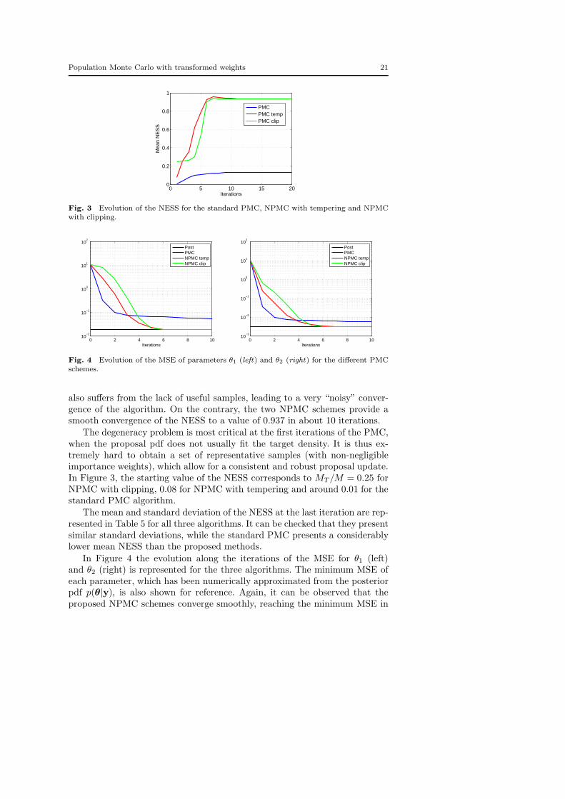
In Figures 3 and 4 numerical results comparing the performance of thethree algorithms (PMC, NPMC with tempering and NPMC with clipping)are displayed. In Figure 3 the evolution of the average NESS along the itera-tions is depicted. It can be observed that the original PMC scheme presentsa low NESS, converging to a value of2 0.131. As a consequence of the degen-eracy problem, the estimates of the variables of interest obtained from thisreduced set of representative samples are often poor, presenting its variancelarge fluctuations along the iterations. Since the proposal density is updatedbased on the set of samples at the previous iteration, the update procedure

2 Note that the NESS ranges between 0 and 1.


0 5 10 15 200

0.2

0.4

0.6

0.8

1

Iterations

Mea

n N

ES

S

PMCPMC tempPMC clip

Fig. 3 Evolution of the NESS for the standard PMC, NPMC with tempering and NPMCwith clipping.

0 2 4 6 8 1010

−2

10−1

100

101

102

Iterations

PostPMCNPMC tempNPMC clip

0 2 4 6 8 1010

−3

10−2

10−1

100

101

102

Iterations

PostPMCNPMC tempNPMC clip

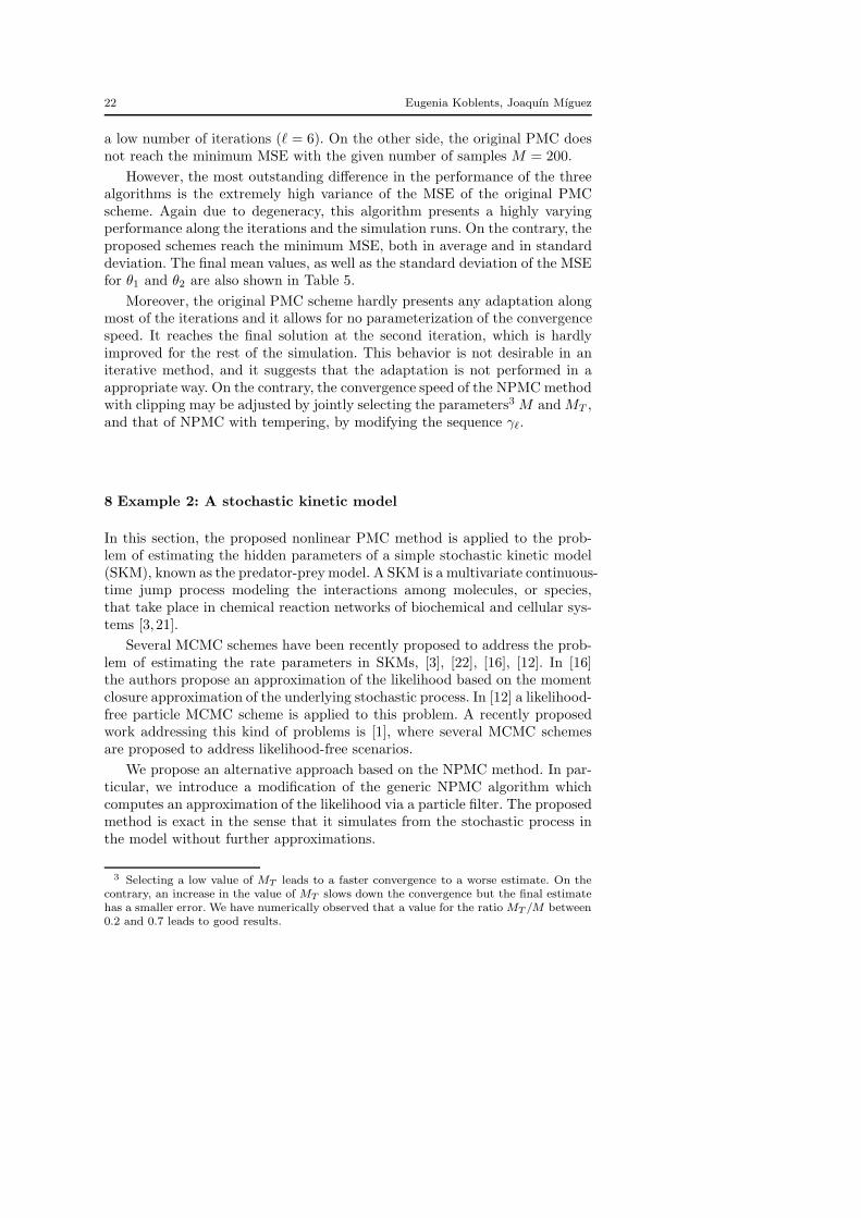
Fig. 4 Evolution of the MSE of parameters θ1 (left) and θ2 (right) for the different PMCschemes.

also suffers from the lack of useful samples, leading to a very “noisy” conver-gence of the algorithm. On the contrary, the two NPMC schemes provide asmooth convergence of the NESS to a value of 0.937 in about 10 iterations.

The degeneracy problem is most critical at the first iterations of the PMC,when the proposal pdf does not usually fit the target density. It is thus ex-tremely hard to obtain a set of representative samples (with non-negligibleimportance weights), which allow for a consistent and robust proposal update.In Figure 3, the starting value of the NESS corresponds to MT/M = 0.25 forNPMC with clipping, 0.08 for NPMC with tempering and around 0.01 for thestandard PMC algorithm.

The mean and standard deviation of the NESS at the last iteration are rep-resented in Table 5 for all three algorithms. It can be checked that they presentsimilar standard deviations, while the standard PMC presents a considerablylower mean NESS than the proposed methods.

In Figure 4 the evolution along the iterations of the MSE for θ1 (left)and θ2 (right) is represented for the three algorithms. The minimum MSE ofeach parameter, which has been numerically approximated from the posteriorpdf p(θ|y), is also shown for reference. Again, it can be observed that theproposed NPMC schemes converge smoothly, reaching the minimum MSE in


a low number of iterations (ℓ = 6). On the other side, the original PMC doesnot reach the minimum MSE with the given number of samples M = 200.

However, the most outstanding difference in the performance of the threealgorithms is the extremely high variance of the MSE of the original PMCscheme. Again due to degeneracy, this algorithm presents a highly varyingperformance along the iterations and the simulation runs. On the contrary, theproposed schemes reach the minimum MSE, both in average and in standarddeviation. The final mean values, as well as the standard deviation of the MSEfor θ1 and θ2 are also shown in Table 5.

Moreover, the original PMC scheme hardly presents any adaptation alongmost of the iterations and it allows for no parameterization of the convergencespeed. It reaches the final solution at the second iteration, which is hardlyimproved for the rest of the simulation. This behavior is not desirable in aniterative method, and it suggests that the adaptation is not performed in aappropriate way. On the contrary, the convergence speed of the NPMC methodwith clipping may be adjusted by jointly selecting the parameters3 M andMT ,and that of NPMC with tempering, by modifying the sequence γℓ.

8 Example 2: A stochastic kinetic model

In this section, the proposed nonlinear PMC method is applied to the prob-lem of estimating the hidden parameters of a simple stochastic kinetic model(SKM), known as the predator-preymodel. A SKM is a multivariate continuous-time jump process modeling the interactions among molecules, or species,that take place in chemical reaction networks of biochemical and cellular sys-tems [3, 21].

Several MCMC schemes have been recently proposed to address the prob-lem of estimating the rate parameters in SKMs, [3], [22], [16], [12]. In [16]the authors propose an approximation of the likelihood based on the momentclosure approximation of the underlying stochastic process. In [12] a likelihood-free particle MCMC scheme is applied to this problem. A recently proposedwork addressing this kind of problems is [1], where several MCMC schemesare proposed to address likelihood-free scenarios.

We propose an alternative approach based on the NPMC method. In par-ticular, we introduce a modification of the generic NPMC algorithm whichcomputes an approximation of the likelihood via a particle filter. The proposedmethod is exact in the sense that it simulates from the stochastic process inthe model without further approximations.

3 Selecting a low value of MT leads to a faster convergence to a worse estimate. On thecontrary, an increase in the value of MT slows down the convergence but the final estimatehas a smaller error. We have numerically observed that a value for the ratio MT /M between0.2 and 0.7 leads to good results.


8.1 Predator-prey model

The Lotka-Volterra, or predator-prey, model is a simple SKM that describesthe time evolution of two species x1 (prey) and x2 (predator), by means ofK = 3 reaction equations: [3, 20]

x1θ1−→ 2x1 prey reproduction

x1 + x2θ2−→ 2x2 predator reproduction

x2θ3−→ ∅ predator death

The k-th reaction takes place stochastically according to its instantaneousrate ak(t) = θkgk (x(t)), where θk > 0 is the constant (yet random) rateparameter and gk(·) is a continuous function of the current state of the sys-tem x(t) = [x1(t), x2(t)]

⊤. We denote by x1(t), x2(t) the nonnegative, integerpopulation of each species at continuous time t. In this simple example, theinstantaneous rates are of the form

a1(t) = θ1x1(t), a2(t) = θ2x1(t)x2(t), a3(t) = θ3x2(t).

The waiting time to the next reaction is exponentially distributed withparameter a0(t) =

∑Kk=1 ak(t), and the probability of each reaction type is

given by ak(t)/a0(t). We denote by x the vector containing the population ofeach species at the occurrence time of each reaction in a time interval t ∈ [0, T ],i.e.,

x = [x⊤(t1),x⊤(t2), . . . ,x

⊤(tR)]⊤,

where R is the total number of reactions and ti ∈ [0, T ], i = 1, ..., R, arethe time instants at which the reactions occur. Assuming that the entirevector x is observed, the likelihood function for the rate parameter vectorθ = [θ1, . . . , θK ]⊤ can be computed analytically [21],

p(x|θ) =K∏

k=1

p(x|θk) =K∏

k=1

θrkk exp

{

−θk

∫ T

0

gk (x(t)) dt

}

, (12)

where rk is the total number of reactions of type k occurred in the time interval[0, T ].

The structure of the likelihood function in (12) allows the selection of aconjugate prior distribution for the rate parameters in the form of independentGamma components, i.e.,

p(θ) =

K∏

k=1

p(θk) =

K∏

k=1

G(θk; ak, bk), (13)

where ak, bk > 0 are the scale and shape parameters of each component,respectively. Thus, the posterior distribution p(θ|x) =

∏Kk=1 p(θk|x) may be

also factorized into a set of independent Gamma components

p(θk|x) = G

(

θk; ak + rk, bk +

∫ T

0

gk (x(t)) dt

)

.


Therefore, in the complete-data scenario (in which x is observed), exact in-ference may be done for each rate constant θk separately. However, makinginference for complex, high-dimensional and discretely observed SKMs (wherex is not fully available) is a challenging problem [3].

Exact stochastic simulation of generic SKMs, and predator-prey models inparticular, can be carried out by the Gillespie algorithm [11]. This procedureallows to draw samples from the prior pdf of the populations, p(x|θ), forarbitrary SKMs.

Although in this work we restrict ourselves to the predator-prey model,which is a simple but representative example of SKM, the proposed algorithmmay be equally applied to the estimation of parameters of SKMs of highercomplexity.

8.2 NPMC algorithm for SKMs

We assume that a set of N noisy observations of the populations of bothspecies are collected at regular time intervals of length ∆, that is, yn = xn +un, n = 1, . . . , N , where xn = [x1(n∆), x2(n∆)]⊤ and un is a Gaussian noisecomponent with zero mean vector and covariance matrix σ2I. We denote thecomplete vector of observations as y = [y⊤

1 , . . . ,y⊤N ]⊤ with dimension 2N × 1.

Thus, the likelihood of the populations x is given by

p (y|x) =N∏

n=1

N(

yn; xn, σ2I)

.

The goal is to approximate the posterior distribution, with density p(θ|y) ∝p(y|θ)p(θ), given the prior pdf p(θ) and the likelihood p(y|θ), using the NPMCmethod.

In this particular problem, the observations y are related to the variablesθ through the random vector x. Indeed, the likelihood of θ has the form

p(y|θ) =

∫

p(y|x)p(x|θ)dx = Ep(x|θ) [p(y|x)] , (14)

where Ep(x|θ)[·] denotes expectation with respect to the pdf in the subscript,and p(y|x, θ) = p(y|x), since the observations are independent of the param-eters θ given the population vector x. As a consequence, the likelihood of theparameters cannot be evaluated exactly. A set of likelihood-free techniqueshave been recently proposed to tackle this kind of problems, which avoid theneed to evaluate the likelihood function [1]. However, in this work we followa different approach which consists in computing an approximation of thelikelihood of p(y|θ).

In principle, it is possible to approximate the integral in (14) as an averageof the likelihoods p(y|x(i)) of a set {x(i)}Ii=1 of exact Monte Carlo samples


from the density p(x|θ), drawn using the Gillespie algorithm, that is,

p(y|θ) ≈1

I

I∑

i=1

p(

y | x(i))

.

This approach, however, is computationally intractable, because it demandsdrawing a huge number of samples I to obtain a useful approximation of thelikelihood p(y|θ), since the probability of generating a trajectory of popula-tions x(i) similar to the observations is extremely low.

To overcome this difficulty, we propose a simple approach based on using astandard particle filter. An approximation for the likelihood of the parametersp(y | θ(i)) may be recursively obtained based on the particle filter approxima-

tion of the posterior of the populations p(x | y, θ(i)). Indeed, the likelihood of

a sample θ(i) can be recursively factorized as

p(

y | θ(i))

=

N∏

n=1

p(

yn | y1:n−1, θ(i))

where each of the terms in the product (with fixed θ = θ(i)) can be approxi-mated via particle filtering (see, e.g., [8] or [5]).

The NPMC method for this application is exact in the sense that it usesexact samples x(i) from the stochastic model generated via the Gillespie al-gorithm, and does not perform any approximation of the stochastic process.Alternative approaches have been proposed which employ a diffusion approxi-mation. However, this approximation has not shown to introduce any improve-ment to our algorithm.

To summarize, the standard importance weights for this application havethe form

w(i)∗ℓ ∝

p(

y | θ(i)ℓ

)

p(

θ(i)ℓ

)

qℓ

(

θ(i)ℓ

) ,

where the likelihood p(y|θ(i)ℓ ) is approximated using a particle filter. The prior

is a product of K independent Gamma components as in Eq. (13) and theproposal is a multivariate normal pdf, as shown in Table 2.

Let us finally remark that, while in this work we have focused on thecomplete-observation scenario, the proposed method is also valid in the par-tially observed case, when only a subset of the species can be observed.

8.3 Computer simulation results

We have applied the NPMC algorithm to the problem of estimating the pos-terior pdf of the constant rate parameters vector θ in a simple predator-preymodel. The true vector of parameter rates which we aim to estimate has beenset to

θ = [0.5, 0.0025, 0.3]⊤.


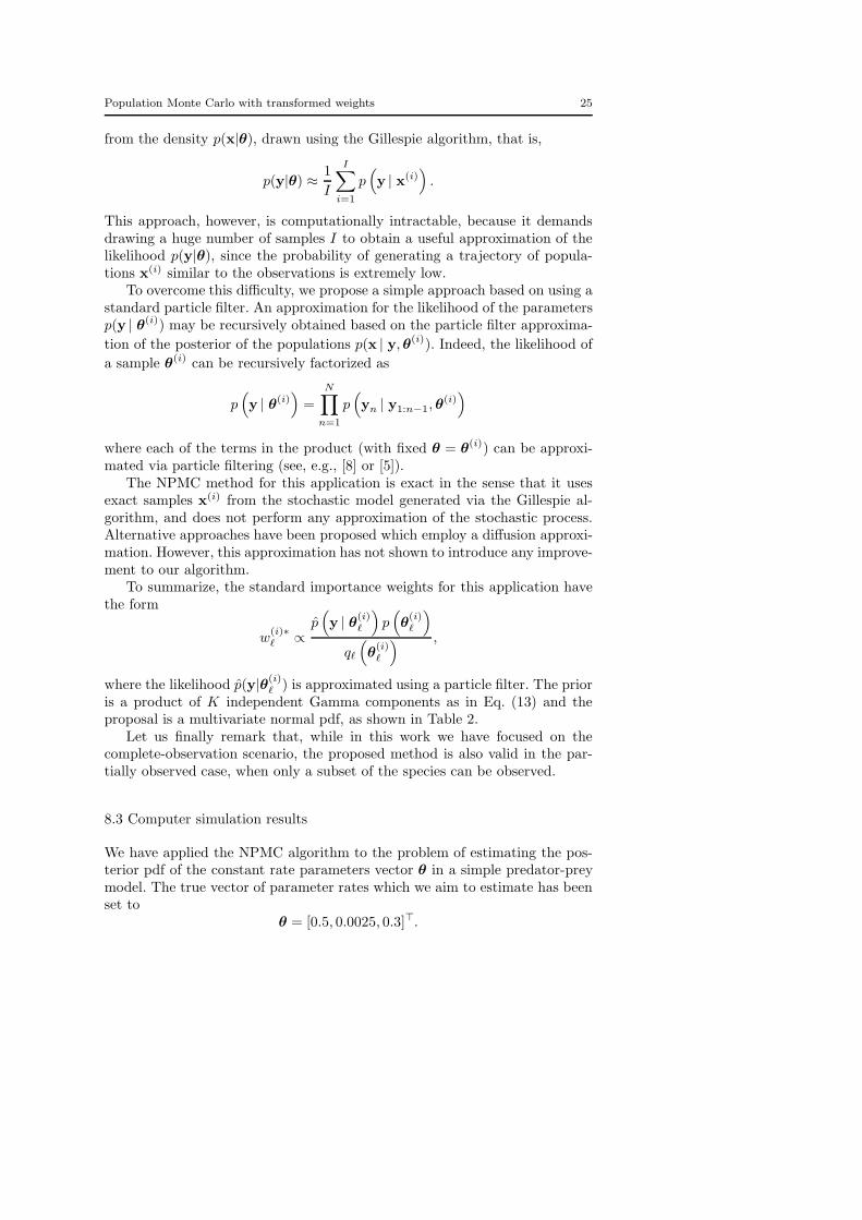
A realization of the populations x has been generated from the prior dis-tribution p(x|θ) with initial populations x(0) = [71, 79]⊤, and a total lengthof T = 40. The observation vector y has been generated with an observationperiod ∆ = 1 and a Gaussian noise variance σ2 = 100.

Figure 5 depicts the time evolution of the true populations of both speciesx, and the corresponding discrete-time noisy observations y. The autoregula-tory behavior of the model can be clearly observed on the graph.

0 10 20 30 40−100

0

100

200

300

400

500

600

Time

Pop

ulat

ions

x1

x2

y1

y2

Fig. 5 Real populations (x) and discrete-time noisy observations (y) in a predator-preymodel.

The parameters of the prior Gamma distribution p(θ) have been chosensuch that the corresponding mean matches the real value of θ and the marginalstandard deviations are [1.25, 0.0065, 0.77]⊤. These priors cover an order ofmagnitude either side of the true value, which represents a vague prior knowl-edge.

The target density for the NPMC algorithm is the posterior pdf, π(θ) =p(θ|y). Despite the low dimension of this problem (K = 3), the importanceweights of the PMC scheme present severe degeneracy, partially due to thelikelihood approximation. In the simulations, we have observed that the im-portance weights present such degeneracy, that, for the NPMC scheme withtempering, the coefficient γℓ must take extremely low values (about 10−4) atthe first iterations in order to balance the weights and obtain a reasonablenumber of effective samples. Besides, the sequence γℓ is hard to design a pri-ori, and it does not guarantee that the resulting sample set leads to accurateestimates. For that reasons, in this example we have restricted our attentionto the hard clipping technique, which does not require the fitting of any pa-rameters and guarantees a baseline ESS. Recall that the NPMC scheme withhard clipping only requires the selection of a unique parameter MT , whichallows to adjust the convergence performance of the algorithm, and does notrequire a precise fitting. In this example, we have chosen MT = M/5, with atotal number of samples M = 500 and L = 10 iterations.

In order to be able to compare the MSE of parameters θk, k = 1, 2, 3, thattake very different values, we additionally define normalized MSEs (NMSE)


0.2 0.4 0.6 0.8−3

−2.5

−2

−1.5

−1

−0.5

NESS

log 10

NM

SE

20

10

0

30 20 10 0 0.2 0.4 0.6 0.8−3

−2.5

−2

−1.5

−1

−0.5

NESS

log 10

NM

SE

20

10

0

40 20 0

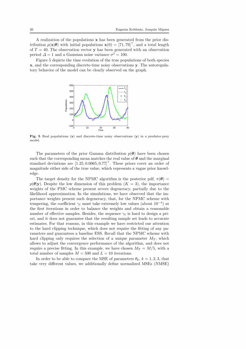
Fig. 6 Left: Average value of log10(NMSE) versus the NESS after the last iteration (L = 10)for each simulation run, with M = 500 samples. The histogram of each variable is alsorepresented. Right: Average value of log10(NMSE) versus the NESS after the last iteration(L = 10) for each simulation run, with M = 500 for 70% of the simulation runs, M = 1000for the 28% of the simulation runs and M = 2000 for 8% of the simulation runs.

as

NMSEk =1

M

M∑

i=1

(

θ(i)k − θkθk

)2

=MSEk

θ2k, k = 1, 2, 3,

and a global error figure as the average NMSE, namely

NMSE =1

K

K∑

k=1

NMSEk.

We have carried out two different experiments. In both experiments wehave performed P = 100 independent simulation runs, with the same trueparameters θ and initial populations x(0), but different (independent) popu-lation and observations vectors x and y in each run.

In the first experiment we considered the same number of samplesM = 500in all the simulation runs of the NPMC algorithm and computed the NESSand the NMSE along the iterations. We observed that a 70% of the simulationruns converged to yield accurate estimates (with low NMSE), while in a 30% ofthe cases, the algorithm produced biased estimates, with considerably higherNMSE and low final NESS (below a 0.3).

In Figure 6 (left) the final values of the logarithm of the NMSE versusthe NESS obtained for each simulation run are depicted, together with thehistograms of both the log10(NMSE) and the NESS. This plot reveals how lowNESS values correspond to high NMSE, and viceversa. This empirical relation-ship is relevant because allows to detect, in practice, whether the algorithmhas converged properly or not.

The second experiment consisted in repeating the simulation of the algo-rithm in those cases which did not yield accurate estimates with M = 500samples, but increasing the number of samples to M = 1000. For this newexperiment, we considered that the algorithm had converged when the final


1 2 3 4 5 6 7 8 9 100

0.1

0.2

0.3

0.4

0.5

Iterations

Mea

n N

ES

S

Ms = 500Ms = 500, 1000, 2000NESS origM

T/M

0 2 4 6 8 1010

−4

10−3

10−2

10−1

100

101

Iterations

Mea

n N

MS

E

M = 500M = 500, 1000, 2000Opt post

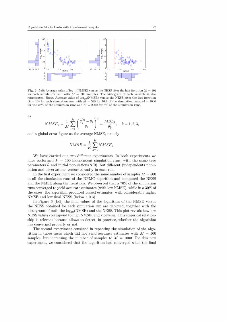
Fig. 7 Left: Evolution of the mean NESS, before and after clipping. The NESS beforeclipping (computed for the standard weights) is labeled NESS orig. Right: Evolution of themean MSE. The lower bound is obtained from the optimal posterior p(θ|x) (labeled Optpost in the figure).

MSE θ1 MSE θ2 MSE θ3 NMSE θ1 NMSE θ2 NMSE θ3 mean NMSE

Prior 1.56 4.42 × 10−5 0.5929 6.25 6.76 6.588 6.533

NPMC clip (1) 9.7× 10−3 53.0 × 10−9 36.8× 10−4 0.03878 0.008484 0.04089 0.02938

NPMC clip (2) 1.4× 10−3 23.46× 10−9 6.38× 10−4 0.005618 0.003754 0.007092 0.005488

Optimal posterior 0.26 × 10−3 5.53 × 10−9 0.881× 10−4 0.00103 0.0008862 0.0009796 0.0009654

Table 6 Final mean MSE and NMSE for the parameters θ1, θ2 and θ3 in experiments 1and 2. The prior and optimal posterior values are included for comparison.

NESS was greater than 0.3. Out of the repeated simulations, 8 cases still didnot converge and the simulations were repeated with M = 2000. Finally, allthe simulation runs obtained a final NESS> 0.3 with a number of particlesM = 500 for the 70% of the cases, M = 1000 for the 22% of the cases andM = 2000 for the 8% of the cases.

In Figure 6 (right) the final values of log10(NMSE) versus the NESS areplotted after repeating the simulations with M = 1000 (22% of the runs) andM = 2000 (8% of the runs). It can be observed that the points with highNMSE are removed and that most points concentrate in the region of highNESS and low NMSE. Also the histograms of NMSE and NESS show howtheir mean values significantly improve.

Figure 7 shows the evolution of the mean NESS and NMSE along theiterations in both experiments. In solid blue lines, the results regarding the firstexperiment are plotted (M = 500 for all simulation runs). In solid red lines,the results of the second experiment are represented (M = 500, M = 1000and M = 2000).

In Figure 7 (left) the evolution of the NESS, Mneffℓ , after the clipping

procedure in both experiments is represented. In both cases it starts froman initial value of MT /M and reaches a final value of about 0.43 in the first


10−1

100

0

5

10

15

20

25

30

35

40

θ1

p(θ1)

p(θ1| x)

p(θ1| y) est

θ1

10−3

10−2

0

1000

2000

3000

4000

5000

6000

7000

8000

θ2

p(θ2)

p(θ2| x)

p(θ2| y) est

θ2

10−1

100

0

10

20

30

40

50

60

70

θ3

p(θ3)

p(θ3| x)

p(θ3| y) est

θ3

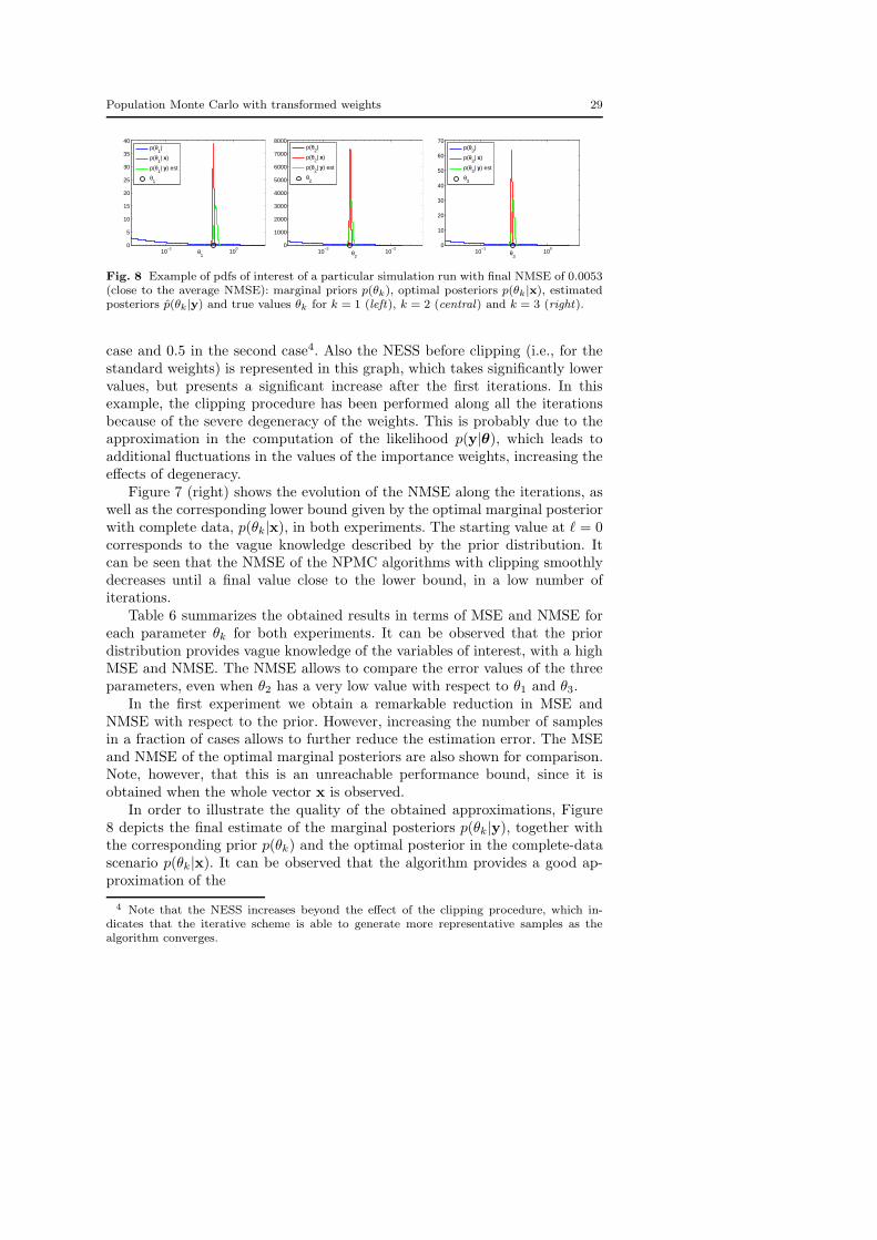
Fig. 8 Example of pdfs of interest of a particular simulation run with final NMSE of 0.0053(close to the average NMSE): marginal priors p(θk), optimal posteriors p(θk|x), estimatedposteriors p(θk|y) and true values θk for k = 1 (left), k = 2 (central) and k = 3 (right).

case and 0.5 in the second case4. Also the NESS before clipping (i.e., for thestandard weights) is represented in this graph, which takes significantly lowervalues, but presents a significant increase after the first iterations. In thisexample, the clipping procedure has been performed along all the iterationsbecause of the severe degeneracy of the weights. This is probably due to theapproximation in the computation of the likelihood p(y|θ), which leads toadditional fluctuations in the values of the importance weights, increasing theeffects of degeneracy.

Figure 7 (right) shows the evolution of the NMSE along the iterations, aswell as the corresponding lower bound given by the optimal marginal posteriorwith complete data, p(θk|x), in both experiments. The starting value at ℓ = 0corresponds to the vague knowledge described by the prior distribution. Itcan be seen that the NMSE of the NPMC algorithms with clipping smoothlydecreases until a final value close to the lower bound, in a low number ofiterations.

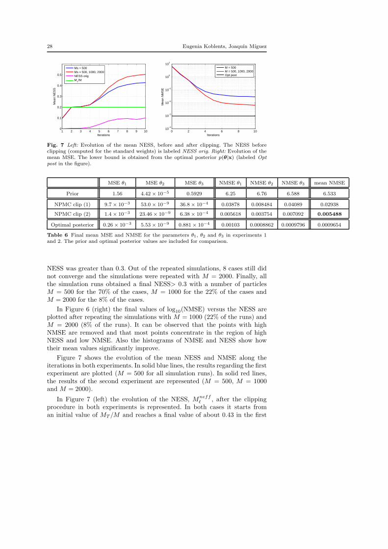
Table 6 summarizes the obtained results in terms of MSE and NMSE foreach parameter θk for both experiments. It can be observed that the priordistribution provides vague knowledge of the variables of interest, with a highMSE and NMSE. The NMSE allows to compare the error values of the threeparameters, even when θ2 has a very low value with respect to θ1 and θ3.

In the first experiment we obtain a remarkable reduction in MSE andNMSE with respect to the prior. However, increasing the number of samplesin a fraction of cases allows to further reduce the estimation error. The MSEand NMSE of the optimal marginal posteriors are also shown for comparison.Note, however, that this is an unreachable performance bound, since it isobtained when the whole vector x is observed.

In order to illustrate the quality of the obtained approximations, Figure8 depicts the final estimate of the marginal posteriors p(θk|y), together withthe corresponding prior p(θk) and the optimal posterior in the complete-datascenario p(θk|x). It can be observed that the algorithm provides a good ap-proximation of the

4 Note that the NESS increases beyond the effect of the clipping procedure, which in-dicates that the iterative scheme is able to generate more representative samples as thealgorithm converges.


9 Conclusion

We have addressed the problem of approximating posterior probability distri-butions by means of random samples. A recently proposed approach to tacklethis problem is the population Monte Carlo method, that consists in iterativelyapproximating a target distribution via an importance sampling scheme. Themain limitation of this algorithm is that is presents severe degeneracy of theimportance weights as the dimension of the model, K, and/or the number ofobservations, N , increase. This leads to a highly varying number of effectivesamples and inaccurate estimates, unless the number of samples is extremelyhigh (which makes the method computationally prohibitive).

We propose to apply a simple procedure in order to guarantee a prescribedESS and a smooth and robust convergence. It consists in applying nonlineartransformations to the standard importance weights in order to reduce theirfluctuations and thus avoid degeneracy. In order to illustrate the applicationof the proposed technique, we have applied it to two examples of differentcomplexity. The first example is a simple GMM, which allows to get insight ofthe performance of the standard PMC scheme, the degeneracy problem andthe behavior of the proposed algorithm.

We have tackled the problem of estimating the set of constant (and ran-dom) rate parameters of a stochastic kinetic model. Even for the relativelysimple predator-prey model that we have studied, this is significantly morecomplex than the GMM example. We have shown extensive simulation resultsthat show how the proposed NPMC scheme can greatly improve the perfor-mance of the standard method.

The convergence of standard PMC algorithms is often justified by theasymptotic convergence of IS (with respect to the number of samples). TheNPMC scheme modifies the importance weights and, hence, the standard the-ory of IS cannot be applied directly. To address this difficulty, we have an-alyzed the convergence of the approximations of integrals computed usingtransformed importance weights and proved that they converge a.s., similarto the results available for standard IS.

Acknowledgements E. K. acknowledges the support of Ministerio de Educacion of Spain(Programa de Formacion de Profesorado Universitario, ref. AP2008-00469). This work hasbeen partially supported by Ministerio de Economıa y Competitividad of Spain (programConsolider-Ingenio 2010 CSD2008-00010 COMONSENS and project DEIPRO TEC2009-14504-C02-01).

A Proof of Lemma 1

As a first step, we seek a tractable upper bound for the difference

∣

∣

∣(f, πM )− (f, πM )

∣

∣

∣=

∣

∣

∣

∣

∣

M∑

i=1

f(θ(i))(

w(i) − w(i))

∣

∣

∣

∣

∣

, (15)


where

w(i) =(ϕM ◦ g)(θ(i))

∑Mj=1(ϕ

M ◦ g)(θ(j))and (16)

w(i) =(ϕM ◦ g)(θ(i))∑M

j=1 g(θ(j))

, (17)

and (ϕM ◦g)(θ) = ϕM (g(θ)) denotes the composition of the functions ϕM and g. Moreover,the constants in the denominators of the weights can be written as integrals with respect tothe random measure

qM (dθ) =1

M

M∑

j=1

δθ(j) (dθ), (18)

namely,M∑

j=1

(ϕM ◦ g)(θ(j)) = M(ϕM ◦ g, qM ) (19)

andM∑

j=1

g(θ(j)) = M(g, qM ). (20)

Substituting (16), (17), (19) and (20), into (15) yields, after straightforward manipulations,

∣

∣

∣(f, πM )− (f, πM )

∣

∣

∣=

∣

∣

∣

∣

∣

1

M

M∑

i=1

f(θ(i))(ϕM ◦ g)(θ(i))(g, qM ) − (ϕM ◦ g, qM )

(ϕM ◦ g, qM )(g, qM )

∣

∣

∣

∣

∣

. (21)

A useful upper bound for the difference of integrals follows quite easily from (21). In partic-

ular, note that |f(θ(i))(ϕM ◦ g)| ≤ ‖f‖∞‖g‖∞, since f, g ∈ B(RK) and ϕM ◦ g ≤ g, whilethe latter inequality also implies that (ϕM ◦ g, qM )(g, qM ) ≥ (ϕM ◦ g, qM )2. Also note that,from the definition of ϕM ,

|(g, qM )− (ϕM ◦ g, qM )| ≤ 1

M

MT∑

k=1

|g(θ(ik))− (ϕM ◦ g)(θ(ik))|

≤ 2MT ‖g‖∞M

. (22)

As a result, we obtain

∣

∣

∣(f, πM )− (f, πM )

∣

∣

∣≤ 2‖f‖∞‖g‖2∞MT

M(ϕM ◦ g, qM )2. (23)

Let c1 > 0 be some arbitrary real constant. From (23),

P

{

∣

∣

∣(f, πM )− (f, πM )

∣

∣

∣≤ MT

Mc1

}

≥ P

{

2‖f‖∞‖g‖2∞MT

M(ϕM ◦ g, qM )2≤ MT

Mc1

}

. (24)

If we choose

c1 =2‖f‖∞‖g‖2∞

(

1a− 1√

2

)2(g, q)2

, (25)

where 1 < a <√2, then substituting (25) into the right hand side of (24) yields

P

{

2‖f‖∞‖g‖2∞MT


Mc1

}

= P

{

(ϕM ◦ g, qM )2 ≥(

1

a− 1√

2

)2

(g, q)2

}

= P

{

(ϕM ◦ g, qM )− 1

a(g, q) ≥ − 1√

2(g, q)

}

,

= P

{

M(ϕM ◦ g, qM )− M

a(g, q) ≥ − M√

2(g, q)

}

, (26)


where the second equality holds because 1a− 1√

2> 0.

Next, consider the expectations Eq [(ϕM ◦g, qM )] and Eq [(g, qM )] = (g, q). Since, |(ϕM ◦g, qM )− (g, qM )| ≤ 2MT ‖g‖∞/M (see Eq. (22)), it follows that

∣

∣

∣Eq

[

(ϕM ◦ g, qM )]

−Eq

[

(g, qM )]∣

∣

∣≤ Eq

[

|(ϕM ◦ g, qM ) − (g, qM )|]

≤ 2MT ‖g‖∞M

.

Therefore, since we have assumed that limM→∞MTM

= 0 and g > 0, there exists Ma suchthat, for all M > Ma,

Eq

[

(ϕM ◦ g, qM )]

>1

aEq

[

(g, qM )]

=1

a(g, q), (27)

and combining Eq. (26) with the inequality (27) we obtain that

P

{

2‖f‖∞‖g‖2∞MT


Mc1

}

≥

P

{

M(ϕM ◦ g, qM )−MEq

[

(ϕM ◦ g, qM )]

≥ − M√2(g, q)

}

. (28)

Since M(ϕM ◦ g, qM ) =∑M

i=1 ϕM (g(θ(i))) is the sum of M independent and bounded

random variables, each of them taking values within the interval (0, ‖g‖∞), it is straightfor-ward to apply Hoeffding’s tail inequality [13] to obtain a lower bound on (28), namely

P

{

M(ϕM ◦ g, qM ) −MEq

[

(ϕM ◦ g, qM )]

≥ − M√2(g, q)

}

≥ 1− exp

{

− (g, q)2

‖g‖2∞M.

}

. (29)

Substituting (29) back into (28), (26) and (24) yields the desired result,

P

{

∣

∣

∣(f, πM )− (f, πM )

∣

∣

∣≤ MT

Mc1

}

≥ 1− exp{

−c′1M}

, (30)

with c′1 =(g,q)2

‖g‖2∞

.

B Proof of Lemma 2

The argument is similar to that of the proof of Lemma 1. Recalling Eqs. (17), (18) and (20)in Appendix A as well as the form of the standard normalized weights,

w(i) =g(θ(i))

M(g, qM ),

it is straightforward to show that

∣

∣

∣(f, πM )− (f, πM )

∣

∣

∣=

1

M(g, qM )

∣

∣

∣

∣

∣

∣

MT∑

k=1

f(θ(ik))(

(ϕM ◦ g)(θ(ik))− g(θ(ik)))

∣

∣

∣

∣

∣

∣

,

which readily yields the upper bound

∣

∣

∣(f, πM )− (f, πM )

∣

∣

∣≤ 2‖f‖∞‖g‖∞MT

M(g, qM ). (31)


Let c2 > 0 be some arbitrary real constant. From (31),

P

{

∣

∣

∣(f, πM )− (f, πM )

∣

∣

∣≤ MT

Mc2

}

≥ P

{

2‖f‖∞‖g‖∞MT

M(g, qM )≤ MT

Mc2

}

(32)

and if we choose

c2 =2‖f‖∞‖g‖∞

(

1− 1√2

)

(g, q),

then

P

{

2‖f‖∞‖g‖∞MT

M(g, qM )≤ MT

Mc2

}

= P

{

(g, qM ) ≥(

1− 1√2

)

(g, q)

}

= P

{

M(g, qM ) −M(g, q) ≥ − M√2(g, q)

}

. (33)

Since (g, q) = Eq[(g, qM )] and (g, qM ) is the sum of M independent, and bounded,random variables taking values within the interval (0, ‖g‖∞] (recall that g > 0), we canreadily apply Hoeffding’s tail inequality [13] on Eq. (33) to obtain

P

{

M(g, qM ) −M(g, q) ≥ − M√2(g, q)

}

≥ 1− exp

{

− (g, q)2

‖g‖2∞M

}

. (34)

Substituting (34) back into (33) and (32) yields the desired result,

P

{

∣

∣

∣(f, πM )− (f, πM )

∣

∣

∣≤ MT

Mc2

}

≥ 1− exp{

−c′2M}

,

where c′2 = (g,q)2

‖g‖2∞

> 0.

C Proof of Lemma 3

The first part of Lemma 3 follows from the combination of Lemmas 1 and 2. We first notethat, from Lemma 1,

P

{

∣

∣

∣(f, πM )− (f, πM )

∣

∣

∣> c1

MT

M

}

< exp{−c′1M} (35)

for sufficiently large M , while Lemma 2 implies

P

{

∣

∣

∣(f, πM ) − (f, πM )

∣

∣

∣> c2

MT

M

}

< exp{−c′2M}, (36)

where c2 = c′2 = (g, q)2/‖g‖2∞. Let c = c1 + c2. Then, since

|(f, πM ) − (f, πM )| ≤ |(f, πM )− (f, πM )|+ |(f, πM )− (f, πM )|,

we trivially obtain that

P

{

∣

∣

∣(f, πM )− (f, πM )

∣

∣

∣> c

MT

M

}

≤ P

{

∣

∣

∣(f, πM ) − (f, πM )

∣

∣

∣+

∣

∣

∣(f, πM )− (f, πM )

∣

∣

∣> c

MT

M

}

.

(37)However, if

∣

∣

∣(f, πM ) − (f, πM )

∣

∣

∣+

∣

∣

∣(f, πM )− (f, πM )

∣

∣

∣> c

MT

M


is true, then

∣

∣

∣(f, πM )− (f, πM )

∣

∣

∣> c1

MT

Mor

∣

∣

∣(f, πM )− (f, πM )

∣

∣

∣> c2

MT

M,

or both jointly, are true. Therefore,

P

{

∣

∣

∣(f, πM )− (f, πM )

∣

∣

∣+

∣

∣

∣(f, πM )− (f, πM )

∣

∣

∣> c

MT

M

}

≤ P

{

∣

∣

∣(f, πM )− (f, πM )

∣

∣

∣> c1

MT

M

}

+P

{

∣

∣

∣(f, πM )− (f, πM )

∣

∣

∣> c2

MT

M

}

≤ exp{

−c′1M}

+ exp{

−c′2M}

= 2 exp

{

− (g, q)2

‖g‖2∞M

}

, (38)

for sufficiently large M , where the second inequality follows from (35) and (36), and theequality is due to the fact that c′1 = c′2.

Combining (37) and (38) yields the first part of Lemma 3, with c′ = (g, q)2/‖g‖2∞.The second part of Lemma 3 follows from a standard Borel-Cantelli argument. Indeed,

let EM be the event in which∣

∣(f, πM )− (f, πM )∣

∣ > cMT

Mholds true. From the first part of

the Lemma,P {EM} < 2 exp

{

−c′M}

,

with c′ > 0, for sufficiently large M (specifically, for all M > Ma, with Ma as in the proofof Lemma 1). Therefore,

∞∑

M=1

P {EM} ≤ Ma +∞∑

M=Ma+1

exp{

−c′M}

< ∞,

because Ma < ∞ and∑∞

M=Ma+1 exp {−c′M} < ∞. As a consequence (see, e.g., [23,

Theorem 2.7]), P {lim sup EM} = 0, which implies that

limM→∞

|(f, πM )− (f, πM )| = 0 a.s.

⊓⊔

References

1. M. Baragatti, A. Grimaud, and D. Pommeret. Likelihood-free parallel tempering. Arxivpreprint arXiv:1108.3423, 2011.

2. T. Bengtsson, P. Bickel, and B. Li. Curse of dimensionaluty revisited: Collapse ofparticle filter in very large scale systems. Probability and statistics: Essay in honour ofDavid A. Freedman, 2:316–334, 2008.

3. R. J. Boys, D. J. Wilkinson, and T. B. L. Kirkwood. Bayesian inference for a discretelyobserved stochastic kinetic model. Statistics and Computing, 18(2):125–135, 2008.

4. M.F. Bugallo, M. Hong, and P.M. Djuric. Marginalized population monte carlo. InAcoustics, Speech and Signal Processing, 2009. ICASSP 2009. IEEE International Con-ference on, pages 2925–2928. IEEE, 2009.

5. J. Mıguez C. S. Maız, E. Molanes-Lopez and P. M. Djuric. A particle filtering scheme forprocessing time series corrupted by outliers. IEEE Transactions on Signal Processing,9(60), September 2012.

6. O. Cappe, R. Douc, A. Guillin, J. M. Marin, and C. P. Robert. Adaptive importancesampling in general mixture classes. Statistics and Computing, 18(4):447–459, 2008.


7. O. Cappe, A. Guillin, J. M. Marin, and C. P. Robert. Population Monte Carlo. Com-putational and Graphical Statistics, 13(4):907–929, 2004.

8. P. M. Djuric and J. Mıguez. Assessment of nonlinear dynamic models by Kolmogorov-Smirnov statistics. IEEE Transactions Signal Processing, 58(10):5069–5079, October2010.

9. R. Douc, A. Guillin, J.M. Marin, and CP Robert. Minimum variance importance sam-pling via population monte carlo. ESAIM: Probability and Statistics, 11(1):427–447,2007 DUDO!!

10. A. Doucet, S. Godsill, and C. Andrieu. On sequential Monte Carlo Sampling methodsfor Bayesian filtering. Statistics and Computing, 10(3):197–208, 2000.

11. D. T. Gillespie. Exact stochastic simulation of coupled chemical reactions. The Journalof Physical Chemistry, 81(25):2340–2361, 1977.

12. A. Golightly and D.J. Wilkinson. Bayesian parameter inference for stochastic biochem-ical network models using particle mcmc. Interface Focus 1. In press, 2011.

13. W. Hoeffding. Probability inequalities of sums of bounded random variables. Journalof the American Statistical Association, 58(301):13–30, March 1963.

14. E. Koblents and J. Mıguez. A population Monte Carlo method for Bayesian inferenceand its application to stochastik kinetic models. In EUSIPCO, 2011.

15. A. Kong, J. S. Liu, and W. H. Wong. Sequential imputations and Bayesian missingdata problems. Journal of the American Statistical Association, 9:278–288, 1994.

16. P. Milner, C.S. Gillespie, and D.J. Wilkinson. Moment closure based parameter inferenceof stochastic kinetic models. Statistics and Computing, pages 1–9, 2006.

17. M. Bugallo P. M. Djuric, B. Shen. Population Monte Carlo methodology a la Gibbssampling. In EUSIPCO, 2011.

18. C. P. Robert and G. Casella. Monte Carlo Statistical Methods. Springer, 2004.19. B. Shen, M.F. Bugallo, and P.M. Djuric. Multiple marginalized population monte carlo.

EUSIPCO, 2010.20. V. Volterra. Fluctuations in the abundance of a species considered mathematically.

Nature, 118:558–560, 1926.21. D. J. Wilkinson. Stochastic Modelling for Systems Biology. Chapman & Hall/CRC,

Mathematical and Computational Biology Series, 2006.22. D.J. Wilkinson. Parameter inference for stochastic kinetic models of bacterial gene

regulation: A bayesian approach to systems biology. (with discussion), in BayesianStatistics, 9, 2011.

23. D. Williams. Probability with Martingales. Cambdridge University Press, Cambridge(UK), 1991.

A population Monte Carlo scheme with transformed weights and its application to stochastic kinetic...

Documents

Transcript of A population Monte Carlo scheme with transformed weights and its application to stochastic kinetic...