a path toward an effective scaling approach for axial

A PATH TOWARD AN EFFECTIVE SCALING APPROACH FOR AXIAL

PISTON MACHINES

A Dissertation

Submitted to the Faculty

of

Purdue University

by

Lizhi Shang

In Partial Fulfillment of the

Requirements for the Degree

of

Doctor of Philosophy

December 2018

Purdue University

West Lafayette, Indiana

ii

THE PURDUE UNIVERSITY GRADUATE SCHOOL

STATEMENT OF DISSERTATION APPROVAL

Dr. Monika Ivantysynova, Chair

Department of Agricultural and Biological Engineering

Dr. Andrea Vacca, Chair


Dr. Farshid Sadeghi

School of Mechanical Engineering

Dr. John Lumkes


Dr. Sadegh Dabiri


Approved by:

Dr. Bernard Engel

Head of the School Graduate Program

iii

To Glorify God.

iv

ACKNOWLEDGMENTS

I would like to first thank my major professor Dr. Monika Ivantysynova, who

gave me the opportunity as being a graduate student at Maha fluid power research

center, who provided me guidance and financial support through the time I pursue

my Ph.D. degree, who encouraged me through her own hardworking and dedication,

who inspired me by demonstrating how the world can be changed through research

and education. I also would like to thank Dr. Andrea Vacca who provided necessary

advice toward my Ph.D. thesis and defense.

I also want to thank my colleges who had work with me. I want to thank Dan

Mizell, and Ashley Busquets, and Shanmukh Sarode, who were working on the pis-

ton/cylinder interface with me. I want to thank Jeremy Beale and Ashkan Darbani

who were working on the slipper/swashplate interface with me. I want to thank Swar-

nava Mukherjee who was working on the cylinder block/valve plate interface with me.

I want to thank Paul Kalbfleisch, Meike Ernst, and Rene Chacon who were working

late with me.

The person who I must thank the most is my wife Fazhi, who trusts and supports

me, loves me and forgives me. Fazhi, thank you for embarking on this exciting

adventure with me.

v

TABLE OF CONTENTS

Page

LIST OF TABLES . . . . . . . . . . . . . . . . . . . . . . . . . . . . . . . . . . viii

LIST OF FIGURES . . . . . . . . . . . . . . . . . . . . . . . . . . . . . . . . . ix

SYMBOLS . . . . . . . . . . . . . . . . . . . . . . . . . . . . . . . . . . . . . xvii

ABBREVIATIONS . . . . . . . . . . . . . . . . . . . . . . . . . . . . . . . . . . xx

ABSTRACT . . . . . . . . . . . . . . . . . . . . . . . . . . . . . . . . . . . . . xxi

1 INTRODUCTION . . . . . . . . . . . . . . . . . . . . . . . . . . . . . . . . 1

1.1 Background . . . . . . . . . . . . . . . . . . . . . . . . . . . . . . . . . 1

1.2 State-of-the-art . . . . . . . . . . . . . . . . . . . . . . . . . . . . . . . 4

1.3 Aims . . . . . . . . . . . . . . . . . . . . . . . . . . . . . . . . . . . . . 9

2 THE SWASHPLATE TYPE AXIAL PISTON MACHINES . . . . . . . . . . 11

2.1 Kinematics . . . . . . . . . . . . . . . . . . . . . . . . . . . . . . . . . 11

2.2 Slipper/swashplate interface . . . . . . . . . . . . . . . . . . . . . . . . 13

2.3 Piston/cylinder interface . . . . . . . . . . . . . . . . . . . . . . . . . . 16

2.4 Cylinder block/valve plate interface . . . . . . . . . . . . . . . . . . . . 18

3 THE PROPOSED PISTON/CYLINDER INTERFACE MODEL . . . . . . . 22

3.1 Introduction to piston/cylinder interface modeling . . . . . . . . . . . . 22

3.2 A backward difference squeeze term in the Reynolds equation . . . . . 24

3.3 Improved FVM fluid domain discretion scheme . . . . . . . . . . . . . . 30

3.4 Physics-based boundaries for fluid film thickness . . . . . . . . . . . . . 36

3.5 Advanced integrated solid body heat transfer model . . . . . . . . . . . 39

3.6 Heat transfer model for compressible fluid . . . . . . . . . . . . . . . . 44

3.7 Experimental validation . . . . . . . . . . . . . . . . . . . . . . . . . . 49

3.8 Conclusion . . . . . . . . . . . . . . . . . . . . . . . . . . . . . . . . . . 58

4 THERMAL BOUNDARIES PREDICTION MODEL . . . . . . . . . . . . . 60

vi

Page

4.1 Introduction to the thermal boundaries . . . . . . . . . . . . . . . . . . 60

4.2 Temperature change via adiabatic compression and expansion . . . . . 65

4.3 Temperature change via heat transfer . . . . . . . . . . . . . . . . . . . 67

4.4 Structure of thermal boundaries prediction model . . . . . . . . . . . . 71

4.5 Multi-physics multi-domain model . . . . . . . . . . . . . . . . . . . . . 72

4.6 Model validation . . . . . . . . . . . . . . . . . . . . . . . . . . . . . . 74

4.7 Sensitivity study . . . . . . . . . . . . . . . . . . . . . . . . . . . . . . 79

4.8 Conclusion . . . . . . . . . . . . . . . . . . . . . . . . . . . . . . . . . . 86

5 THE SCALING OF PHYSICAL PHENOMENA IN AXIAL PISTON MA-CHINES . . . . . . . . . . . . . . . . . . . . . . . . . . . . . . . . . . . . . . 87

5.1 Linear scaling method (conventional approach) . . . . . . . . . . . . . . 87

5.2 Analysis of fundamental physics of lubricating interfaces . . . . . . . . 91

5.2.1 Fluid pressure distribution . . . . . . . . . . . . . . . . . . . . . 91

5.2.2 Solid body elastic deformation . . . . . . . . . . . . . . . . . . . 92

5.2.3 Multi-domain heat transfer . . . . . . . . . . . . . . . . . . . . . 98

5.3 Findings and scaling guides . . . . . . . . . . . . . . . . . . . . . . . 110

5.4 Conclusions . . . . . . . . . . . . . . . . . . . . . . . . . . . . . . . . 113

6 A PATH TOWARD AN EFFECTIVE PISTON/CYLINDER INTERFACESCALING . . . . . . . . . . . . . . . . . . . . . . . . . . . . . . . . . . . . 114

6.1 Piston/cylinder interface fluid film . . . . . . . . . . . . . . . . . . . . 114

6.2 Clearance and piston guide length study . . . . . . . . . . . . . . . . 117

6.3 Piston material study (temperature adaptive piston design) . . . . . . 121

6.4 Clearance-performance relationship at different sizes . . . . . . . . . . 127

6.5 Groove profile for down-scaled piston/cylinder interface . . . . . . . . 130

6.6 Conclusion . . . . . . . . . . . . . . . . . . . . . . . . . . . . . . . . . 135

7 A PATH TOWARD AN EFFECTIVE CYLINDER BLOCK/VALVE PLATEINTERFACE SCALING . . . . . . . . . . . . . . . . . . . . . . . . . . . . 137

7.1 Fluid film in cylinder block/valve plate interface . . . . . . . . . . . . 137

7.2 Cylinder block/valve plate interface design parameters . . . . . . . . 139

vii

Page

7.3 The width of the sealing land for different sizes . . . . . . . . . . . . 145

7.4 A nonlinear scaling approach . . . . . . . . . . . . . . . . . . . . . . . 148

7.5 Conclusion . . . . . . . . . . . . . . . . . . . . . . . . . . . . . . . . . 155

8 A PATH TOWARD AN EFFECTIVE SLIPPER/SWASHPLATE INTER-FACE SCALING . . . . . . . . . . . . . . . . . . . . . . . . . . . . . . . . 156

8.1 slipper/swashplate interface balance factor . . . . . . . . . . . . . . . 156

8.2 The width of the slipper sealing land . . . . . . . . . . . . . . . . . . 157

8.3 The inner diameter of the slipper sealing land . . . . . . . . . . . . . 160

8.4 Conclusion . . . . . . . . . . . . . . . . . . . . . . . . . . . . . . . . . 164

9 CONCLUSION AND OUTLOOK . . . . . . . . . . . . . . . . . . . . . . . 166

REFERENCES . . . . . . . . . . . . . . . . . . . . . . . . . . . . . . . . . . . 170

VITA . . . . . . . . . . . . . . . . . . . . . . . . . . . . . . . . . . . . . . . . 174

viii

LIST OF TABLES

Table Page

3.1 Operating condition for EHD pump temperature distribution measurement. 51

4.1 Operating temperatures of HT , MT , and LT . . . . . . . . . . . . . . . . 62

4.2 Required fluid properties. . . . . . . . . . . . . . . . . . . . . . . . . . . . 72

4.3 Required operating conditions. . . . . . . . . . . . . . . . . . . . . . . . . . 74

4.4 Operating conditions of the comparison study. . . . . . . . . . . . . . . . . 75

4.5 Set #2, outlet and case flow temperature comparison at 100% displacement 79





4.10 Set #4, outlet and case flow temperature comparison at 100% and 10%displacement . . . . . . . . . . . . . . . . . . . . . . . . . . . . . . . . . . 84

5.1 Summary of unit sizes and operating conditions. . . . . . . . . . . . . . . . 88

5.2 Summary of operating conditions with scaled fluid viscosity. . . . . . . . . 96

5.3 Summary of operating conditions with scaled fluid viscosity, scaled fluidconductivity, and scaled solid conductivity. . . . . . . . . . . . . . . . . . 107

6.1 Summary of operating conditions. . . . . . . . . . . . . . . . . . . . . . . 119

6.2 Summary of operating conditions. . . . . . . . . . . . . . . . . . . . . . . 122

7.1 Summary of unit sizes and operating conditions. . . . . . . . . . . . . . . 140

8.1 Summary of unit sizes and operating conditions. . . . . . . . . . . . . . . 157

ix

LIST OF FIGURES

Figure Page

1.1 Three lubricating interfaces in swashplate type axial piston machines. . . . 1

1.2 The two opposing physical phenomena. . . . . . . . . . . . . . . . . . . . . 2

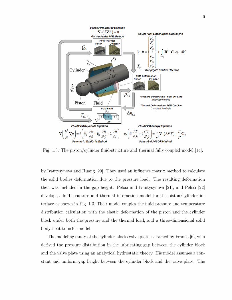
1.3 The piston/cylinder fluid-structure and thermal fully coupled model [14]. . 6

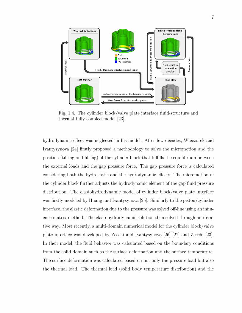
1.4 The cylinder block/valve plate interface fluid-structure and thermal fullycoupled model [23]. . . . . . . . . . . . . . . . . . . . . . . . . . . . . . . . 7

1.5 The slipper/swashplate interface fluid-structure and thermal fully coupledmodel [28]. . . . . . . . . . . . . . . . . . . . . . . . . . . . . . . . . . . . 8

2.1 Kinematic relationship for the swashplate type axial piston machine. . . . 12

2.2 Illustration of piston spinning motion. . . . . . . . . . . . . . . . . . . . . 13

2.3 Components of the total axial force from the piston. . . . . . . . . . . . . . 14

2.4 Slipper free body diagram. . . . . . . . . . . . . . . . . . . . . . . . . . . . 15

2.5 Piston free body diagram. . . . . . . . . . . . . . . . . . . . . . . . . . . . 17

2.6 Cylinder block free body diagram. . . . . . . . . . . . . . . . . . . . . . . . 18

3.1 The structure of the piston/cylinder interface fluid structure and thermalinteraction model. . . . . . . . . . . . . . . . . . . . . . . . . . . . . . . . . 23

3.2 Generalized piston/cylinder lubricating gap . . . . . . . . . . . . . . . . . 24

3.3 Percentage of penetration area. . . . . . . . . . . . . . . . . . . . . . . . . 26

3.4 Measured cylinder bore surface profile. . . . . . . . . . . . . . . . . . . . . 26

3.5 EHD squeeze impacts on bearing function. . . . . . . . . . . . . . . . . . . 28

3.6 Newton-Raphson method to find piston position that fulfills the force balance.28

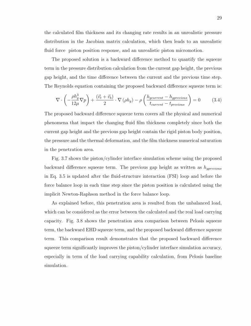
3.7 Piston/cylinder interface simulation scheme using the proposed backwarddifference squeeze term. . . . . . . . . . . . . . . . . . . . . . . . . . . . . 30

3.8 Bearing function simulation comparison. . . . . . . . . . . . . . . . . . . . 31

3.9 Finite volume discretization for pressure distribution calculation. . . . . . . 32

3.10 Fluid density change with pressure. . . . . . . . . . . . . . . . . . . . . . . 32

x

Figure Page

3.11 Fluid viscosity change with pressure. . . . . . . . . . . . . . . . . . . . . . 33

3.12 Gap pressure distribution comparison at 90-degree shaft angle. . . . . . . . 34

3.13 Gap pressure spike comparison at 90-degree shaft angle. . . . . . . . . . . 34

3.14 Single piston/cylinder interface energy dissipation comparison. . . . . . . . 35

3.15 Single piston/cylinder interface energy dissipation comparison of the gapheight estimation method between Pelosis and the proposed. . . . . . . . . 38

3.16 Pressure distribution comparison of the gap height estimation methodbetween Pelosis and the proposed. . . . . . . . . . . . . . . . . . . . . . . . 39

3.17 Instantaneous piston/cylinder interface mesh relative position. . . . . . . . 41

3.18 Node to node heat flux. . . . . . . . . . . . . . . . . . . . . . . . . . . . . 42

3.19 The piston temperature convergence check for the previous model. . . . . . 43

3.20 The piston temperature convergence check for the advanced heat transfermodel. . . . . . . . . . . . . . . . . . . . . . . . . . . . . . . . . . . . . . . 44

3.21 Fluid enthalpy changes over pressure and temperature. . . . . . . . . . . . 45

3.22 Three-dimensional finite volume structure for fluid domain (a), and thefinite volume definition (b) [14] . . . . . . . . . . . . . . . . . . . . . . . . 48

3.23 Three dimensional fluid domain temperature distribution comparison. . . . 49

3.24 The EHD test pump. . . . . . . . . . . . . . . . . . . . . . . . . . . . . . . 50

3.25 The EHD pump sensor positions. . . . . . . . . . . . . . . . . . . . . . . . 51

3.26 EHD measurement vs. simulation at 2.5mm from D.C.. . . . . . . . . . . . 52



3.29 EHD measurement vs. simulation at 14.33mm from D.C.. . . . . . . . . . 53







xi

Figure Page

4.1 Definition of the control volumes in swashplate type axial piston machines 61

4.2 Simulation results for HT , MT , and LT . . . . . . . . . . . . . . . . . . . . 62

4.3 Schematic of the heat and mass transfer in axial piston machines. . . . . . 63

4.4 Simplified schematic of the heat and mass transfer in in axial piston machines.64

4.5 An example compression process in the displacement chamber volume. . . 65

4.6 Simplified three-volume scheme for heat transfer. . . . . . . . . . . . . . . 68

4.7 Pump flow temperatures prediction model solution scheme. . . . . . . . . . 71

4.8 An multi-physics multi-domain model to predict swashplate type axialpiston machine performance. . . . . . . . . . . . . . . . . . . . . . . . . . . 73

4.9 Type I and type II fluid properties. . . . . . . . . . . . . . . . . . . . . . . 75

4.10 Set #1, flow temperatures comparison at 100% displacement. . . . . . . . 76

4.11 Set #1, flow temperatures comparison at 80% displacement. . . . . . . . . 76




4.15 Outlet flow temperature for different normalized leakage the normalizedmechanical losses. . . . . . . . . . . . . . . . . . . . . . . . . . . . . . . . . 85

4.16 Case flow temperature for different normalized leakage the normalizedmechanical losses. . . . . . . . . . . . . . . . . . . . . . . . . . . . . . . . . 85

5.1 Normalized piston/cylinder interface performance for different sizes. . . . . 89

5.2 Normalized cylinder block/valve plate interface performance for differentsizes. . . . . . . . . . . . . . . . . . . . . . . . . . . . . . . . . . . . . . . . 90

5.3 Normalized slipper/swashplate interface performance for different sizes. . . 90

5.4 An arbitrary lubricating gap. . . . . . . . . . . . . . . . . . . . . . . . . . 92

5.5 Normalized piston/cylinder interface performance for different sizes (noheat transfer, scaled viscosity). . . . . . . . . . . . . . . . . . . . . . . . . 97

5.6 Normalized cylinder block/valve plate interface performance for differentsizes (no heat transfer, scaled viscosity). . . . . . . . . . . . . . . . . . . . 97

5.7 Normalized slipper/swashplate interface performance for different sizes (noheat transfer, scaled viscosity). . . . . . . . . . . . . . . . . . . . . . . . . 98

xii

Figure Page

5.8 Normalized piston/cylinder interface performance for different sizes (scaledviscosity). . . . . . . . . . . . . . . . . . . . . . . . . . . . . . . . . . . . . 99

5.9 Normalized cylinder block/valve plate interface performance for differentsizes (scaled viscosity). . . . . . . . . . . . . . . . . . . . . . . . . . . . . 100

5.10 Normalized slipper/swashplate interface performance for different sizes(scaled viscosity). . . . . . . . . . . . . . . . . . . . . . . . . . . . . . . . 100

5.11 Demonstration of solid body temperature comparison for different sizes. . 101

5.12 Piston temperature distribution comparison for different sizes (scaled vis-cosity). . . . . . . . . . . . . . . . . . . . . . . . . . . . . . . . . . . . . . 101

5.13 Cylinder block temperature distribution comparison for different sizes (scaledviscosity). . . . . . . . . . . . . . . . . . . . . . . . . . . . . . . . . . . . 102

5.14 Slipper temperature distribution comparison for different sizes (scaled vis-cosity). . . . . . . . . . . . . . . . . . . . . . . . . . . . . . . . . . . . . . 103

5.15 Piston temperature distribution comparison for different sizes (scaled vis-cosity, scaled fluid and solid conductivity). . . . . . . . . . . . . . . . . . 107

5.16 Cylinder block temperature distribution comparison for different sizes (scaledviscosity, scaled fluid and solid conductivity). . . . . . . . . . . . . . . . 108

5.17 Slipper temperature distribution comparison for different sizes (scaled vis-cosity, scaled fluid and solid conductivity). . . . . . . . . . . . . . . . . . 108

5.18 Normalized piston/cylinder interface performance for different sizes (scaledviscosity, scaled fluid and solid conductivity). . . . . . . . . . . . . . . . 109

5.19 Normalized cylinder block/valve plate interface performance for differentsizes (scaled viscosity, scaled fluid and solid conductivity). . . . . . . . . 109

5.20 Normalized slipper/swashplate interface performance for different sizes(scaled viscosity, scaled fluid and solid conductivity). . . . . . . . . . . . 110

6.1 Inclined piston in cylinder bore forming the fluid film. . . . . . . . . . . . 115

6.2 Film thickness for the unwrapped gap without pressure and thermal de-formations. . . . . . . . . . . . . . . . . . . . . . . . . . . . . . . . . . . 115

6.3 The resulting change of film thickness ∆hg def pdue to pressure deformation.116

6.4 The resulting change of film thickness ∆hg def th due to thermal deformation.117

6.5 Piston guide length. . . . . . . . . . . . . . . . . . . . . . . . . . . . . . 118

6.6 Piston guide length and clearance influence on piston/cylinder interfaceperformance at OC #1. . . . . . . . . . . . . . . . . . . . . . . . . . . . 119

xiii

Figure Page




6.10 Baseline piston design vs Bi-material piston design. . . . . . . . . . . . . 122

6.11 Thermal deformation comparison between the baseline design and the bi-material design. . . . . . . . . . . . . . . . . . . . . . . . . . . . . . . . . 123

6.12 baseline piston vs bi-material design at 100◦C half speed. . . . . . . . . . 124

6.13 baseline piston vs bi-material design at 100◦C full speed. . . . . . . . . . 124

6.14 baseline piston vs bi-material design at 52◦C half speed. . . . . . . . . . 125

6.15 baseline piston vs bi-material design at 52◦C full speed. . . . . . . . . . . 125

6.16 baseline piston vs bi-material design at -20◦C half speed. . . . . . . . . . 125

6.17 baseline piston vs bi-material design at -20◦C full speed. . . . . . . . . . 126

6.18 Clearance influence on piston/cylinder interface performance at differencesizes at OC #1. . . . . . . . . . . . . . . . . . . . . . . . . . . . . . . . . 127




6.22 Mass flow in and out of the groove control volume. . . . . . . . . . . . . 130

6.23 Groove cells and boundary cells in the fluid domain grid. . . . . . . . . . 131

6.24 Pressure distribution calculation scheme with groove profile. . . . . . . . 132

6.25 Two types of groove profiles. . . . . . . . . . . . . . . . . . . . . . . . . . 133

6.26 Grooved piston/cylinder interface performance comparing to the baselinedesign for the small size with different clearance at OC #1. . . . . . . . . 133


xiv

Figure Page



7.1 Fluid film in cylinder block/valve plate interface. . . . . . . . . . . . . . 138

7.2 Cylinder block gap dimensions. . . . . . . . . . . . . . . . . . . . . . . . 138

7.3 Width of the sealing land edges b. . . . . . . . . . . . . . . . . . . . . . . 139

7.4 Small thin fluid film area comparing to the whole fluid domain in cylinderblock/valve plate interface. . . . . . . . . . . . . . . . . . . . . . . . . . . 141

7.5 Width of the sealing land impact on interface performance at OC #1 and#2. . . . . . . . . . . . . . . . . . . . . . . . . . . . . . . . . . . . . . . . 142

7.6 Width of the sealing land impact on interface performance at OC #3 and#4. . . . . . . . . . . . . . . . . . . . . . . . . . . . . . . . . . . . . . . . 142

7.7 Thickness of the valve plate and the end case d. . . . . . . . . . . . . . . 142

7.8 Length of the cylinder block canal channel l. . . . . . . . . . . . . . . . . 143

7.9 Thickness of the valve plate and end case assembly impact on interfaceperformance at OC #1 and #2. . . . . . . . . . . . . . . . . . . . . . . . 144

7.10 Thickness of the valve plate and end case assembly impact on interfaceperformance at OC #3 and #4. . . . . . . . . . . . . . . . . . . . . . . . 144

7.11 Length of the canal channel impact on interface performance at OC #1and #2. . . . . . . . . . . . . . . . . . . . . . . . . . . . . . . . . . . . . 145

7.12 Length of the canal channel impact on interface performance at OC #3and #4. . . . . . . . . . . . . . . . . . . . . . . . . . . . . . . . . . . . . 145

7.13 The normalized power loss, the normalized leakage, and the normalizedunsupported load change with the sealing land edge width for differentsizes at OC #1. . . . . . . . . . . . . . . . . . . . . . . . . . . . . . . . . 146



xv

Figure Page


7.17 An example of a nonlinearly scaled cylinder block running surface. . . . . 149

7.18 Simulated performances of nonlinearly up-scaled cylinder block/valve plateinterface OC #1. . . . . . . . . . . . . . . . . . . . . . . . . . . . . . . . 150




7.22 Simulated performances of nonlinearly down-scaled cylinder block/valveplate interface OC #1. . . . . . . . . . . . . . . . . . . . . . . . . . . . . 153




8.1 Design parameters of the slipper/swashplate interface. . . . . . . . . . . 157

8.2 Normalized power loss and leakage change with the width of the slippersealing land at OC #1. . . . . . . . . . . . . . . . . . . . . . . . . . . . . 158




8.6 Normalized power loss and leakage change with the slipper sealing landinner diameter at OC #1. . . . . . . . . . . . . . . . . . . . . . . . . . . 161


xvi

Figure Page



8.10 Energy efficiency difference of linearly scaled and nonlinearly scaled slip-per/swashplate interface from the baseline. . . . . . . . . . . . . . . . . . 163

xvii

SYMBOLS

A area

b width

C constitutive matrix

cp heat capacity

d diameter

E elastic modulus

F force

FaK axial inertia force

FB external force on block

FDB displacement chamber pressure force on block

FDK displacement chamber pressure force on piston

FG slipper axial load

FHD slipper hold down force

FK piston external force

FKB force from piston to cylinder block

FRK total resultant force from slipper

FSB reaction force on block

FSK reaction force on piston

FTB piston axial friction on block

FTG slipper friction

FTK piston axial friction

FωG slipper centrifugal force

FωK piston-slipper assembly centrifugal force

H enthalpy

xviii

HK piston maximum stroke

h specific enthalpy

hg gap height

l length

lG distance from slipper running surface to ball joint center

lSG distance from slipper COM to ball joint center

MB external moment on block

MDB moment due to displacement chamber pressure force on block

MG slipper external moment

MK piston external moment

MKB moment from piston to cylinder block

MSB reaction moment on block

MTB moment due to piston axial friction on block

MωG moment due to slipper centrifugal force

m mass flow rate

m mass

M heat transfer matrix

n rotational speed

P power

p pressure

Q volumetric flow rate

q heat flux

q rate of heat flux

q vector of heat flux

S entropy

sK piston stroke

s specific entropy

T temperature

t time

xix

T vector of temperature

U strain energy

V volume

u nodal displacement

VNF applied load potential energy

v velocity

V velocity vector

vfluid specific volume

w normal velocity

wt weighting factor

β swashplate angle

Γ diffusion coefficient

ε strain

κ heat transfer coefficient

λ linear scaling factor

µ viscosity

ν Poisson’s ratio

Π potential energy

ρ viscosity

σ stress

ΦD dissipation

φ shaft angle

ω shaft speed

xx

ABBREVIATIONS

avg average

B block

b bottom surface

DC displacement chamber

E east neighbor cell

e east cell wall

EHD elasto-hydrodynamic

FVM finite volume method

G slipper

IDC inner dead center

K piston

N north neighbor cell

n north cell wall

ODC outer dead center

S south neighbor cell

s south cell wall

t top surface

W west neighbor cell

w west cell wall

0 original size

xxi

ABSTRACT

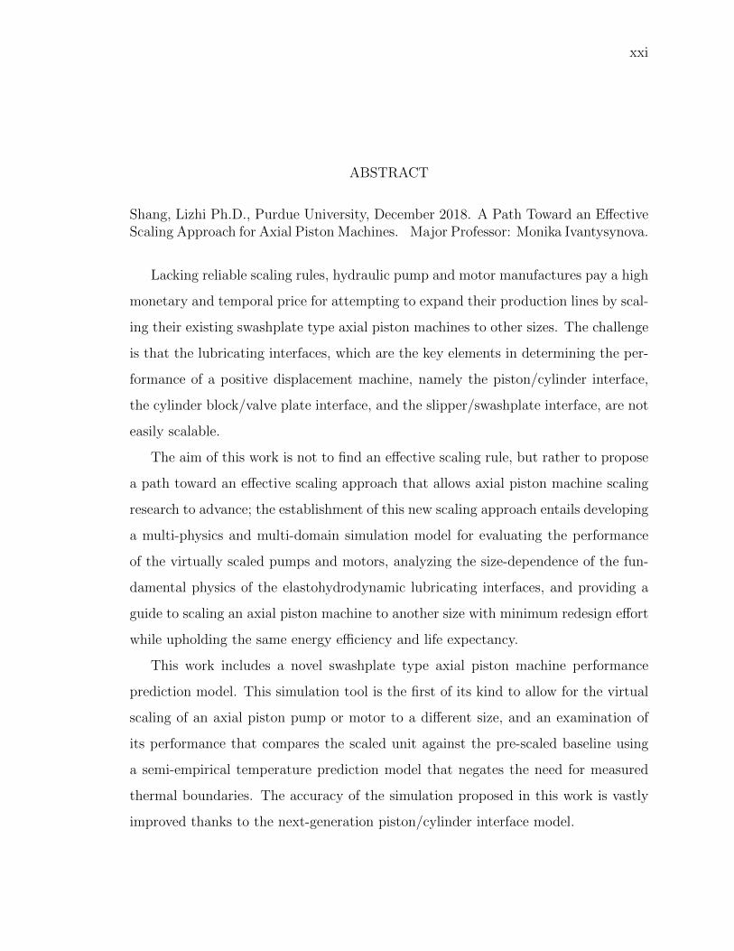
Shang, Lizhi Ph.D., Purdue University, December 2018. A Path Toward an EffectiveScaling Approach for Axial Piston Machines. Major Professor: Monika Ivantysynova.

Lacking reliable scaling rules, hydraulic pump and motor manufactures pay a high

monetary and temporal price for attempting to expand their production lines by scal-

ing their existing swashplate type axial piston machines to other sizes. The challenge

is that the lubricating interfaces, which are the key elements in determining the per-

formance of a positive displacement machine, namely the piston/cylinder interface,

the cylinder block/valve plate interface, and the slipper/swashplate interface, are not

easily scalable.

The aim of this work is not to find an effective scaling rule, but rather to propose

a path toward an effective scaling approach that allows axial piston machine scaling

research to advance; the establishment of this new scaling approach entails developing

a multi-physics and multi-domain simulation model for evaluating the performance

of the virtually scaled pumps and motors, analyzing the size-dependence of the fun-

damental physics of the elastohydrodynamic lubricating interfaces, and providing a

guide to scaling an axial piston machine to another size with minimum redesign effort

while upholding the same energy efficiency and life expectancy.

This work includes a novel swashplate type axial piston machine performance

prediction model. This simulation tool is the first of its kind to allow for the virtual

scaling of an axial piston pump or motor to a different size, and an examination of

its performance that compares the scaled unit against the pre-scaled baseline using

a semi-empirical temperature prediction model that negates the need for measured

thermal boundaries. The accuracy of the simulation proposed in this work is vastly

improved thanks to the next-generation piston/cylinder interface model.

xxii

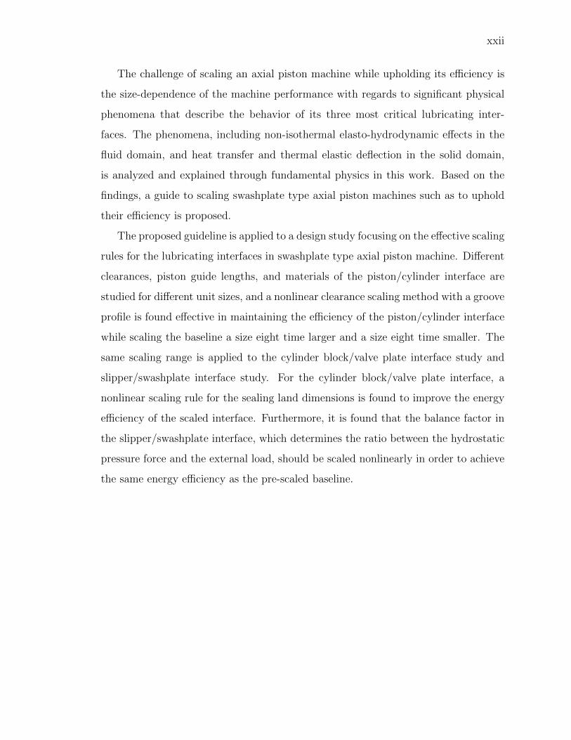
The challenge of scaling an axial piston machine while upholding its efficiency is

the size-dependence of the machine performance with regards to significant physical

phenomena that describe the behavior of its three most critical lubricating inter-

faces. The phenomena, including non-isothermal elasto-hydrodynamic effects in the

fluid domain, and heat transfer and thermal elastic deflection in the solid domain,

is analyzed and explained through fundamental physics in this work. Based on the

findings, a guide to scaling swashplate type axial piston machines such as to uphold

their efficiency is proposed.

The proposed guideline is applied to a design study focusing on the effective scaling

rules for the lubricating interfaces in swashplate type axial piston machine. Different

clearances, piston guide lengths, and materials of the piston/cylinder interface are

studied for different unit sizes, and a nonlinear clearance scaling method with a groove

profile is found effective in maintaining the efficiency of the piston/cylinder interface

while scaling the baseline a size eight time larger and a size eight time smaller. The

same scaling range is applied to the cylinder block/valve plate interface study and

slipper/swashplate interface study. For the cylinder block/valve plate interface, a

nonlinear scaling rule for the sealing land dimensions is found to improve the energy

efficiency of the scaled interface. Furthermore, it is found that the balance factor in

the slipper/swashplate interface, which determines the ratio between the hydrostatic

pressure force and the external load, should be scaled nonlinearly in order to achieve

the same energy efficiency as the pre-scaled baseline.

1

1. INTRODUCTION

1.1 Background

Fluid power actuation and driving systems are widely utilized in industrial appli-

cations. Thanks to their high power density in comparison to other systems, great

compactness of high-performance hydraulic systems is achievable. Among different

types of hydrostatic pumps and motors, swashplate type axial piston machines are

dominating the market of high pressure applications such as agriculture, construction,

forestry, mining, aerospace and manufacturing due to their high operating pressure,

variable displacement operation, great efficiency, superior compactness, and good re-

liability.

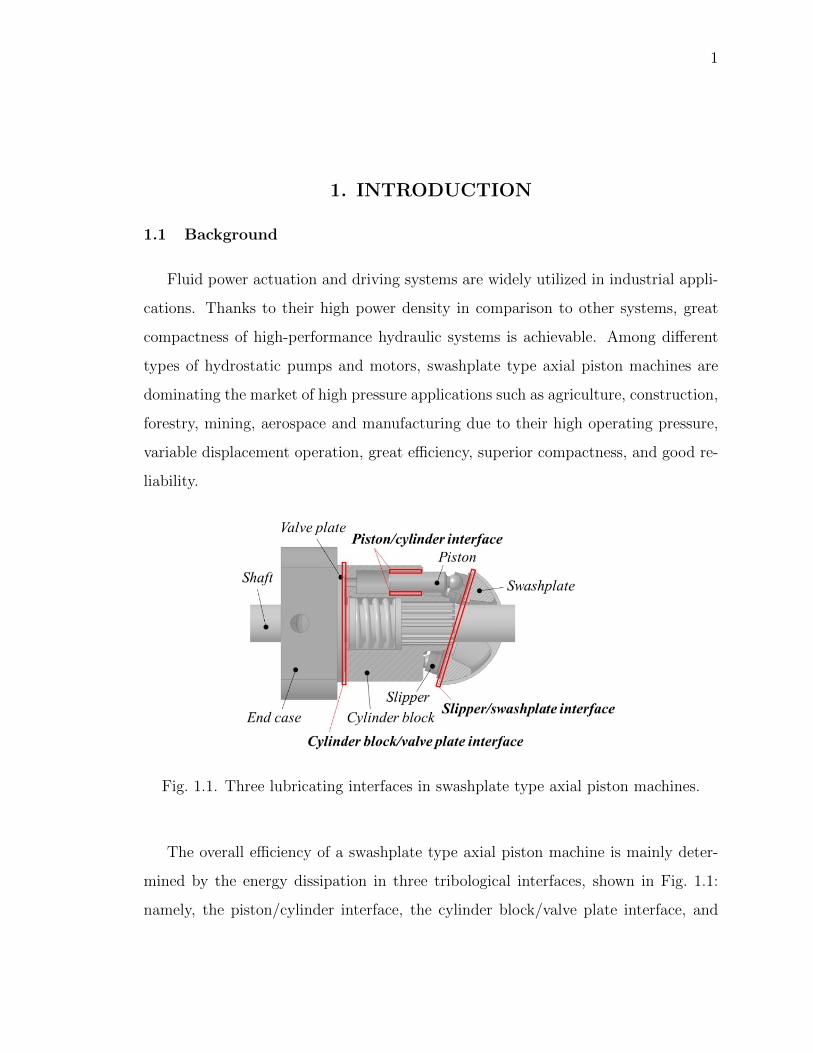
Fig. 1.1. Three lubricating interfaces in swashplate type axial piston machines.

The overall efficiency of a swashplate type axial piston machine is mainly deter-

mined by the energy dissipation in three tribological interfaces, shown in Fig. 1.1:

namely, the piston/cylinder interface, the cylinder block/valve plate interface, and

2

the slipper/swashplate interface. The energy dissipation of these three main lubri-

cating interfaces is due to the viscous shear of the working fluid, which takes on two

forms.

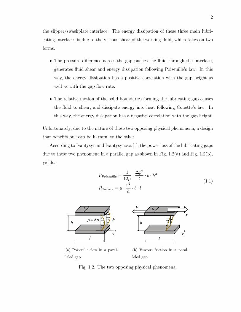
• The pressure difference across the gap pushes the fluid through the interface,

generates fluid shear and energy dissipation following Poiseuille’s law. In this

way, the energy dissipation has a positive correlation with the gap height as

well as with the gap flow rate.

• The relative motion of the solid boundaries forming the lubricating gap causes

the fluid to shear, and dissipate energy into heat following Couette’s law. In

this way, the energy dissipation has a negative correlation with the gap height.

Unfortunately, due to the nature of these two opposing physical phenomena, a design

that benefits one can be harmful to the other.

According to Ivantysyn and Ivantysynova [1], the power loss of the lubricating gaps

due to these two phenomena in a parallel gap as shown in Fig. 1.2(a) and Fig. 1.2(b),

yields:

PPoiseuille =1

12µ· ∆p2

l· b · h3

PCouette = µ · v2

h· b · l

(1.1)

(a) Poiseuille flow in a paral-

leled gap.

(b) Viscous friction in a paral-

leled gap.

Fig. 1.2. The two opposing physical phenomena.

3

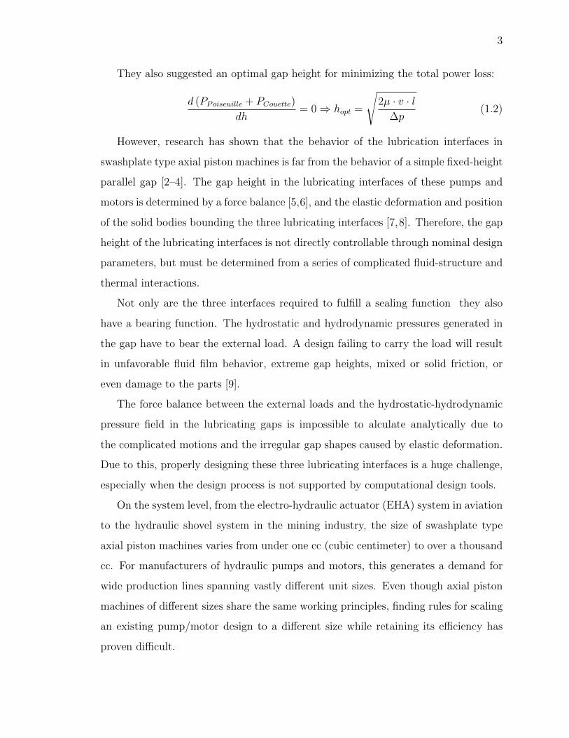
They also suggested an optimal gap height for minimizing the total power loss:

d (PPoiseuille + PCouette)

dh= 0⇒ hopt =

√2µ · v · l

∆p(1.2)

However, research has shown that the behavior of the lubrication interfaces in

swashplate type axial piston machines is far from the behavior of a simple fixed-height

parallel gap [2–4]. The gap height in the lubricating interfaces of these pumps and

motors is determined by a force balance [5,6], and the elastic deformation and position

of the solid bodies bounding the three lubricating interfaces [7,8]. Therefore, the gap

height of the lubricating interfaces is not directly controllable through nominal design

parameters, but must be determined from a series of complicated fluid-structure and

thermal interactions.

Not only are the three interfaces required to fulfill a sealing function they also

have a bearing function. The hydrostatic and hydrodynamic pressures generated in

the gap have to bear the external load. A design failing to carry the load will result

in unfavorable fluid film behavior, extreme gap heights, mixed or solid friction, or

even damage to the parts [9].

The force balance between the external loads and the hydrostatic-hydrodynamic

pressure field in the lubricating gaps is impossible to alculate analytically due to

the complicated motions and the irregular gap shapes caused by elastic deformation.

Due to this, properly designing these three lubricating interfaces is a huge challenge,

especially when the design process is not supported by computational design tools.

On the system level, from the electro-hydraulic actuator (EHA) system in aviation

to the hydraulic shovel system in the mining industry, the size of swashplate type

axial piston machines varies from under one cc (cubic centimeter) to over a thousand

cc. For manufacturers of hydraulic pumps and motors, this generates a demand for

wide production lines spanning vastly different unit sizes. Even though axial piston

machines of different sizes share the same working principles, finding rules for scaling

an existing pump/motor design to a different size while retaining its efficiency has

proven difficult.

4

1.2 State-of-the-art

Series of pumps and motors that differ in size but share the same design do exist

in the axial piston machine categories. Designers and manufacturers found that the

maximum shaft speed of pumps and motors of any size is restricted by the maximum

viscous shear, which is generated by the relative sliding velocity in the tribological

interfaces. Ivantysyn and Ivantysynova [1] suggested the sliding velocity between the

cylinder block and the valve plate should be kept between three to five meter per

second for any size of pumps and motors.

By maintaining the sliding velocity between the moving parts while scaling, the

scaled swashplate type axial piston machine follows the linear scaling rule:

V (λ) = λ3 · Vo

m(λ) = λ3 ·mo

(1.3)

where λ is the linear scaling factor. The rotational speed, as mentioned before, scales

by the reciprocal of the linear scaling factor λ:

n(λ) = λ−1 · no (1.4)

Via this rule of thumb, well-designed units are often scaled to other sizes in order

to extend the market range. However, to achieve the pre-scaled performance in terms

of the energy efficiency and the service lifetime, the required trial-and-error design

process is both financially and temporally expensive.

In order to understand the size-dependent performance of the swashplate type

axial piston machine, a tool that allow for evaluating the efficiency of the pumps and

motors is required.

Merritt [10] parameterized the energy efficiency of hydraulic pumps and motors

through an empirical model, which uses the operating pressure and operating speed

as input variables. However, the coefficients used in his model vary with different unit

designs and unit sizes, and are therefore not scalable. The friction and leakage losses

of the three major lubricating interfaces of such units were calculated analytically

5

under the assumption of rigid body and fixed gap height by Manring, Ivantysyn,

and Ivantysynova [1, 3, 4, 11, 12]. On the basis of these analyses, their work also

suggests an optimal gap height for these interfaces with regards to minimizing losses

[1]. However, the scaling rule that was derived from these loss models is limited by its

failure to account for fundamental physical phenomena, including the non-isothermal

fluid properties, hydrodynamic effects, elastic deformations, heat transfer, and the

interactions between all of the above. In order to find a more effective scaling rule for

swashplate type axial piston machines, a detailed model is required one that allows

for analyzing the performance of the three lubricating interfaces.

The discovery of the thermoelastohydrodynamics of the three lubricating inter-

faces all starts from the Reynolds equation [13], which was derived from the Navier-

Stokes equations and the conservation of mass. Nevertheless, since the kinematics and

dynamics of the three lubricating interfaces are different, the modeling researches of

the three lubricating interfaces were divided into three branches.

Piston/cylinder interface modeling study starts since van der Kolk [15], who con-

ducted the first numerical fluid pressure distribution simulation in the piston/cylinder

gap. The piston/cylinder interface was simplified into a tilt journal bearing in his

model. The piston motion was firstly considered in the pressure distribution calcu-

lation by Yamaguchi [16]. Ivantysynova [17] firstly introduced a non-isothermal fluid

model for the piston/cylinder interface. She coupled the Reynolds equation with the

energy equation, to calculate the temperature field in the piston/cylinder interface

according to energy dissipation from viscous shear. The fluid viscosity in her model

is a function of pressure and temperature. Fang and Shirahashi [18] firstly presented

a methodology to determine the piston position inside of the cylinder bore by looking

for a position that fulfills the equilibrium between the fluid pressure force and the

external load. Olem [19] proposed an iterative method to solve the piston micro mo-

tion, which allows the external load to be balanced by the fluid film considering the

additional hydrodynamic pressure force from the piston micro motion. The first elas-

tohydrodynamic gap flow simulation for the piston/cylinder interface was proposed

6

Fig. 1.3. The piston/cylinder fluid-structure and thermal fully coupled model [14].

by Ivantysynova and Huang [20]. They used an influence matrix method to calculate

the solid bodies deformation due to the pressure load. The resulting deformation

then was included in the gap height. Pelosi and Ivantysynova [21], and Pelosi [22]

develop a fluid-structure and thermal interaction model for the piston/cylinder in-

terface as shown in Fig. 1.3, Their model couples the fluid pressure and temperature

distribution calculation with the elastic deformation of the piston and the cylinder

block under both the pressure and the thermal load, and a three-dimensional solid

body heat transfer model.

The modeling study of the cylinder block/valve plate is started by Franco [6], who

derived the pressure distribution in the lubricating gap between the cylinder block

and the valve plate using an analytical hydrostatic theory. His model assumes a con-

stant and uniform gap height between the cylinder block and the valve plate. The

7

Fig. 1.4. The cylinder block/valve plate interface fluid-structure andthermal fully coupled model [23].

hydrodynamic effect was neglected in his model. After few decades, Wieczorek and

Ivantysynova [24] firstly proposed a methodology to solve the micromotion and the

position (tilting and lifting) of the cylinder block that fulfills the equilibrium between

the external loads and the gap pressure force. The gap pressure force is calculated

considering both the hydrostatic and the hydrodynamic effects. The micromotion of

the cylinder block further adjusts the hydrodynamic element of the gap fluid pressure

distribution. The elastohydrodynamic model of cylinder block/valve plate interface

was firstly modeled by Huang and Ivantysynova [25]. Similarly to the piston/cylinder

interface, the elastic deformation due to the pressure was solved off-line using an influ-

ence matrix method. The elastohydrodynamic solution then solved through an itera-

tive way. Most recently, a multi-domain numerical model for the cylinder block/valve

plate interface was developed by Zecchi and Ivantysynova [26] [27] and Zecchi [23].

In their model, the fluid behavior was calculated based on the boundary conditions

from the solid domain such as the surface deformation and the surface temperature.

The surface deformation was calculated based on not only the pressure load but also

the thermal load. The thermal load (solid body temperature distribution) and the

8

surface temperature were solved through a three-dimensional heat transfer model.

As shown in Fig. 1.4, their model solves the fluid-structure and thermal interaction

problem in iterative scheme.

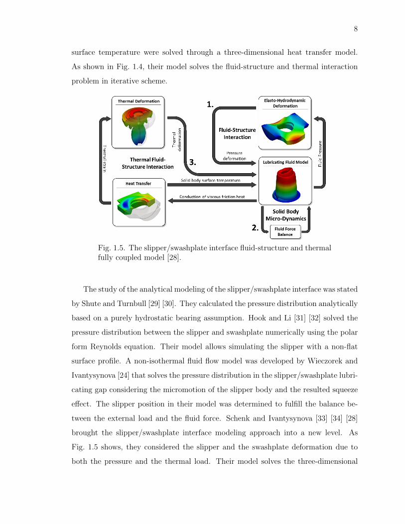
Fig. 1.5. The slipper/swashplate interface fluid-structure and thermalfully coupled model [28].

The study of the analytical modeling of the slipper/swashplate interface was stated

by Shute and Turnbull [29] [30]. They calculated the pressure distribution analytically

based on a purely hydrostatic bearing assumption. Hook and Li [31] [32] solved the

pressure distribution between the slipper and swashplate numerically using the polar

form Reynolds equation. Their model allows simulating the slipper with a non-flat

surface profile. A non-isothermal fluid flow model was developed by Wieczorek and

Ivantysynova [24] that solves the pressure distribution in the slipper/swashplate lubri-

cating gap considering the micromotion of the slipper body and the resulted squeeze

effect. The slipper position in their model was determined to fulfill the balance be-

tween the external load and the fluid force. Schenk and Ivantysynova [33] [34] [28]

brought the slipper/swashplate interface modeling approach into a new level. As

Fig. 1.5 shows, they considered the slipper and the swashplate deformation due to

both the pressure and the thermal load. Their model solves the three-dimensional

9

solid body temperature distribution of the slipper and the swashplate in a heat trans-

fer model.

1.3 Aims

Motivated by the inefficiencies of the current scaling methods, the great compu-

tational and experimental cost of the current scaling process, as well as the huge po-

tential of a more effective scaling procedure, the aim of this work is to propose a path

toward a novel scaling approach that allows axial piston machine scaling research to

advance through the development of a multi-physics multi-domain simulation model

for evaluating the performance of the virtually scaled pumps and motors, through

analysis of the size-dependent performance of the elastohydrodynamic lubricating in-

terfaces via fundamental physics, and through providing a guide axial piston machine

scaling with minimum redesign effort while upholding the energy efficiency and life

expectancy of the unit.

This global aim leads to the formulation of the following research objectives:

• Creation of an accurate multi-physics multi-domain swashplate type axial piston

machine performance prediction tool which can be used without the need for

steady state measurement data.

• Analysis of the size-dependence of non-isothermal elasto-hydrodynamic effects

in the lubricating interface fluid domain, and of heat transfer and elastic defor-

mation in the solid domain.

• Guide on how to scale a swashplate type axial piston machine such as to uphold

its efficiency.

These objectives are met by:

• Developing a next-generation piston/cylinder interface simulation model via

high-fidelity implementation of physical effects using a robust numerical algo-

rithm (Chapter 3). The simulation results of the proposed model are compared

10

to the previous model, and to measurement. The comparison proves the sig-

nificant improvement on model accuracy the proposed simulation tool has to

offer.

• Proposing a semi-empirical thermal boundaries prediction model which calcu-

lates the temperature in the outlet flow and case flow from the pump and motor

design, and from the simulated efficiency of the lubricating gap model. Unlike

the previous model, the proposed model calculates the temperature change due

to compression/expansion separately from the heat generation/transfer (Chap-

ter 4). This proposed model is validated against over three hundred steady-state

measurements.

• Analyzing fundamental physical effects as they pertain to scaling. Each phys-

ical phenomenon, such as the hydrostatic/hydrodynamic effects in lubricating

interfaces, the elastic deformation under both pressure and thermal loads, and

the heat transfer/generation in both fluid and solid domain, is found to be

either scalable (follows the linear scaling rule, i.e. does not contribute to ef-

ficiency changes of the unit when scaling), or non-scalable (does not follow

the linear scaling rule, and modifies the unit’s efficiency). The findings are

also demonstrated using the proposed multi-physics, multi-domain axial piston

pump model (Chapter 5).

• Proposing a general guide for scaling a swashplate type axial piston machine in

order to compensate for the non-scalable physical effects. (Chapter 5).

• Conducting case studies of all three lubricating interfaces for three different

unit sizes at multiple operating conditions to demonstrate the potential of the

proposed scaling guide, and to propose a preliminary nonlinear scaling rule

that is proven to be more effective than the conventional approach. (Chapter 6,

Chapter 7, and Chapter 8)

11

2. THE SWASHPLATE TYPE AXIAL PISTON

MACHINES

The kinematics and the dynamics of swashplate type axial piston machines must be

defined precisely in order to study the behavior of the three lubricating interfaces in

term of the piston/cylinder interface, the cylinder block/valve plate interface, and the

slipper/swashplate interface.

In this chapter, the kinematics of swashplate type axial piston machines is derived

from the geometrical dimensions. Furthermore, the dynamic loading conditions for

each lubricating interface are also explained in detail.

2.1 Kinematics

As the core component of the fluid power system, the swashplate type axial piston

machine converts the mechanic power and the fluid power in both directions depends

on its working mode. In pumping mode, the shaft torque rotates the cylinder block

against the opposing torque due to the pressure force in the displacement chambers

applying on the inclined swashplate through the piston/slipper assembly. The fluid,

therefore, is displaced from the low-pressure input port to the high-pressure output

port. In motoring mode, the pressure force in the displacement chambers applies on

the inclined swashplate as a driving torque, drive the cylinder block together with

the shaft rotating against the torque load on the shaft.

The kinematic relationship for the swashplate type axial piston machine is shown

in Fig. 2.1. A global Cartesian coordinate system is used in Fig. 2.1. The origin

of the coordinate system locates at where the shaft axis crosses the virtual plane

which all the ball joint centers lay on. The positive z pointing along the shaft axis

toward the swashplate, the positive y pointing toward the outer dead center (ODC),

12

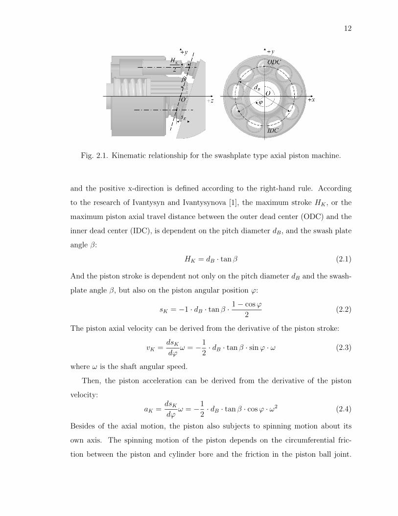
Fig. 2.1. Kinematic relationship for the swashplate type axial piston machine.

and the positive x-direction is defined according to the right-hand rule. According

to the research of Ivantysyn and Ivantysynova [1], the maximum stroke HK , or the

maximum piston axial travel distance between the outer dead center (ODC) and the

inner dead center (IDC), is dependent on the pitch diameter dB, and the swash plate

angle β:

HK = dB · tan β (2.1)

And the piston stroke is dependent not only on the pitch diameter dB and the swash-

plate angle β, but also on the piston angular position ϕ:

sK = −1 · dB · tan β · 1− cosϕ

2(2.2)

The piston axial velocity can be derived from the derivative of the piston stroke:

vK =dsKdϕ

ω = −1

2· dB · tan β · sinϕ · ω (2.3)

where ω is the shaft angular speed.

Then, the piston acceleration can be derived from the derivative of the piston

velocity:

aK =dsKdϕ

ω = −1

2· dB · tan β · cosϕ · ω2 (2.4)

Besides of the axial motion, the piston also subjects to spinning motion about its

own axis. The spinning motion of the piston depends on the circumferential fric-

tion between the piston and cylinder bore and the friction in the piston ball joint.

13

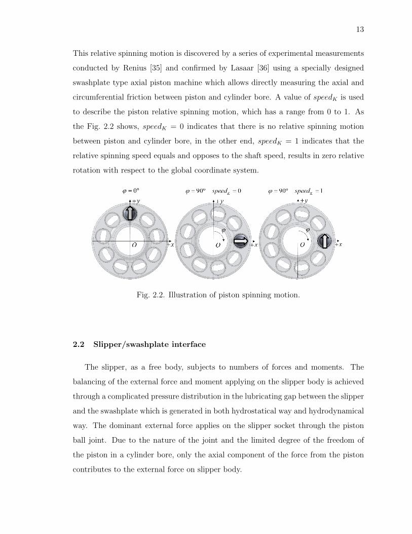
This relative spinning motion is discovered by a series of experimental measurements

conducted by Renius [35] and confirmed by Lasaar [36] using a specially designed

swashplate type axial piston machine which allows directly measuring the axial and

circumferential friction between piston and cylinder bore. A value of speedK is used

to describe the piston relative spinning motion, which has a range from 0 to 1. As

the Fig. 2.2 shows, speedK = 0 indicates that there is no relative spinning motion

between piston and cylinder bore, in the other end, speedK = 1 indicates that the

relative spinning speed equals and opposes to the shaft speed, results in zero relative

rotation with respect to the global coordinate system.

Fig. 2.2. Illustration of piston spinning motion.

2.2 Slipper/swashplate interface

The slipper, as a free body, subjects to numbers of forces and moments. The

balancing of the external force and moment applying on the slipper body is achieved

through a complicated pressure distribution in the lubricating gap between the slipper

and the swashplate which is generated in both hydrostatical way and hydrodynamical

way. The dominant external force applies on the slipper socket through the piston

ball joint. Due to the nature of the joint and the limited degree of the freedom of

the piston in a cylinder bore, only the axial component of the force from the piston

contributes to the external force on slipper body.

14

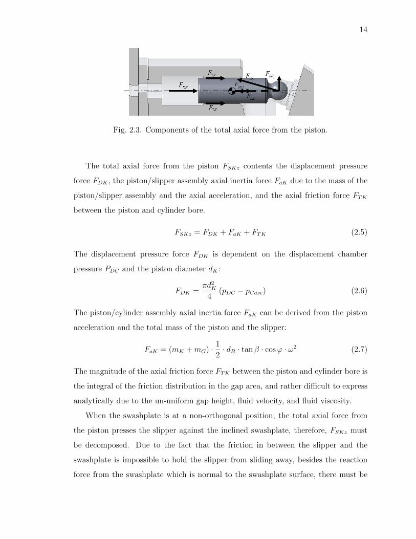
Fig. 2.3. Components of the total axial force from the piston.

The total axial force from the piston FSKz contents the displacement pressure

force FDK , the piston/slipper assembly axial inertia force FaK due to the mass of the

piston/slipper assembly and the axial acceleration, and the axial friction force FTK

between the piston and cylinder bore.

FSKz = FDK + FaK + FTK (2.5)

The displacement pressure force FDK is dependent on the displacement chamber

pressure PDC and the piston diameter dK :

FDK =πd2K

4(pDC − pCase) (2.6)

The piston/cylinder assembly axial inertia force FaK can be derived from the piston

acceleration and the total mass of the piston and the slipper:

FaK = (mK +mG) · 1

2· dB · tan β · cosϕ · ω2 (2.7)

The magnitude of the axial friction force FTK between the piston and cylinder bore is

the integral of the friction distribution in the gap area, and rather difficult to express

analytically due to the un-uniform gap height, fluid velocity, and fluid viscosity.

When the swashplate is at a non-orthogonal position, the total axial force from

the piston presses the slipper against the inclined swashplate, therefore, FSKz must

be decomposed. Due to the fact that the friction in between the slipper and the

swashplate is impossible to hold the slipper from sliding away, besides the reaction

force from the swashplate which is normal to the swashplate surface, there must be

15

an additional force holding the slipper at the position, which is the fluid pressure

distribution in the piston/cylinder lubricating gap. Therefore, the total axial force

from piston FSKz can be decomposed into two components, FSK , which is normal to

the swashplate surface, and FSKy, which is perpendicular to the piston axis. Since

the direction of both components of FSKz are fixed, the magnitude of both forces can

be derived from the swashplate angle.

FSK =FSKzcos β

FSKy = FSKz · tan β

(2.8)

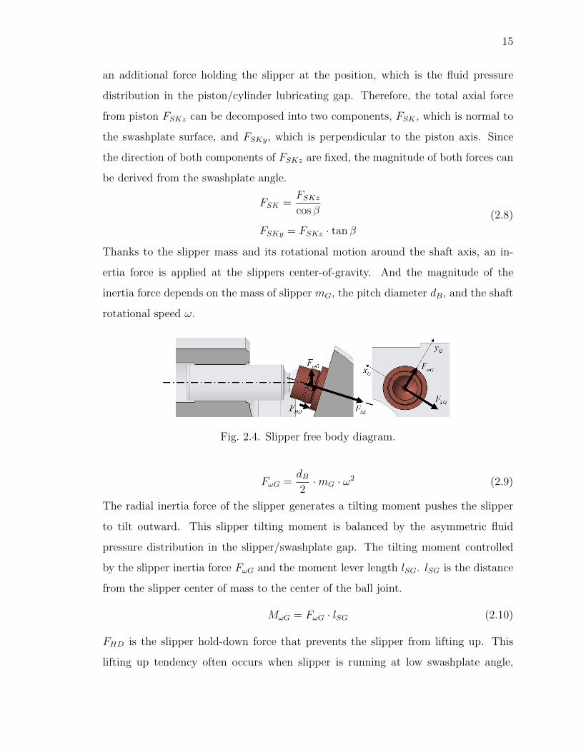
Thanks to the slipper mass and its rotational motion around the shaft axis, an in-

ertia force is applied at the slippers center-of-gravity. And the magnitude of the

inertia force depends on the mass of slipper mG, the pitch diameter dB, and the shaft

rotational speed ω.

Fig. 2.4. Slipper free body diagram.

FωG =dB2·mG · ω2 (2.9)

The radial inertia force of the slipper generates a tilting moment pushes the slipper

to tilt outward. This slipper tilting moment is balanced by the asymmetric fluid

pressure distribution in the slipper/swashplate gap. The tilting moment controlled

by the slipper inertia force FωG and the moment lever length lSG. lSG is the distance

from the slipper center of mass to the center of the ball joint.

MωG = FωG · lSG (2.10)

FHD is the slipper hold-down force that prevents the slipper from lifting up. This

lifting up tendency often occurs when slipper is running at low swashplate angle,

16

low pressure, and high speed. At this situation, the hydrodynamic pressure in the

gap together with the slipper inertia tilting moment overbalances the low pressure

force in the displacement chamber. An additional assistance is necessary to limit the

slipper gap height to prevent large leakage. The slipper hold-down force FHD can

be provided by a spring that located between the slipper retainer and the cylinder

block, or a fixed slipper hold down mechanism, which provided the hold-down force

only when the slipper and swashplate exceeds the nominal design clearance.

The viscous friction between the slipper and swashplate FTG also acts as an exter-

nal load on the slipper body. The magnitude of the friction, however, is the integral

of the local viscous shear over the slipper running surface area, and is rather difficult

to express analytically due to the un-uniform gap height, fluid velocity, and fluid vis-

cosity. The slipper/swashplate friction is always parallel to the slipper surface. The

friction induces another tilting moment that can be calculated from the friction FTG,

and the distance between the piston/slipper ball joint center to the slipper running

surface lG.

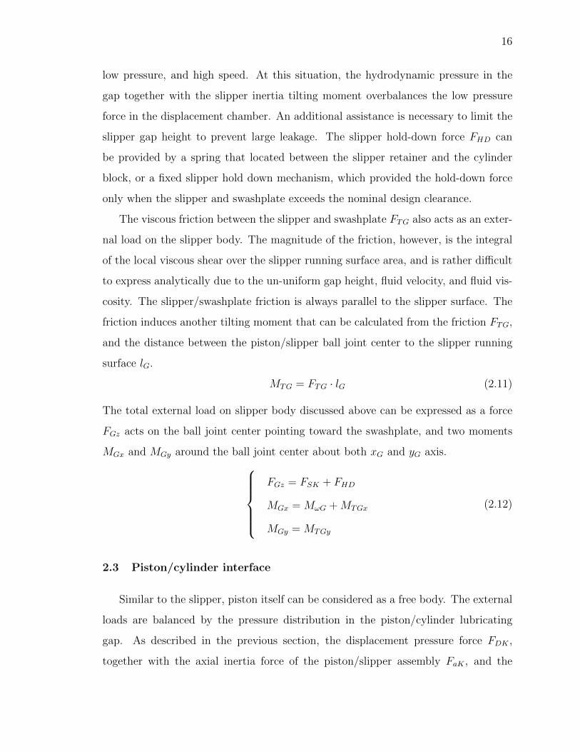
MTG = FTG · lG (2.11)

The total external load on slipper body discussed above can be expressed as a force

FGz acts on the ball joint center pointing toward the swashplate, and two moments

MGx and MGy around the ball joint center about both xG and yG axis.FGz = FSK + FHD

MGx = MωG +MTGx

MGy = MTGy

(2.12)

2.3 Piston/cylinder interface

Similar to the slipper, piston itself can be considered as a free body. The external

loads are balanced by the pressure distribution in the piston/cylinder lubricating

gap. As described in the previous section, the displacement pressure force FDK ,

together with the axial inertia force of the piston/slipper assembly FaK , and the

17

axial friction FTK between piston and cylinder bore, push the piston/slipper assembly

axially against the inclined swashplate. This total axial force FSKx = FDK+FaK+FTK

is decomposed into two components FSKand FSKy. FSK is balanced by the pressure

distribution in slipper/swashplate interface through the piston slipper ball joint. Since

FSKy cannot be balanced from the slipper side, it is considered as an external force

applies at the piston slipper ball joint center, pointing to the positive y-direction in

the global Cartesian coordinate system.

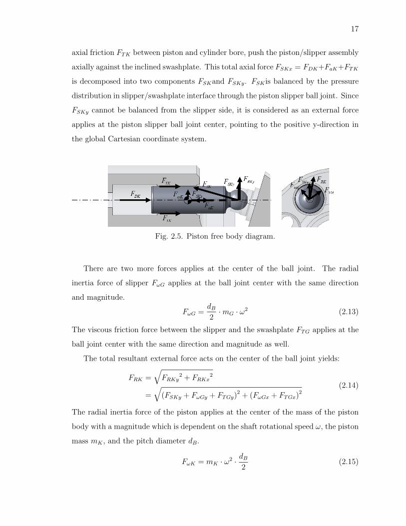
Fig. 2.5. Piston free body diagram.

There are two more forces applies at the center of the ball joint. The radial

inertia force of slipper FωG applies at the ball joint center with the same direction

and magnitude.

FωG =dB2·mG · ω2 (2.13)

The viscous friction force between the slipper and the swashplate FTG applies at the

ball joint center with the same direction and magnitude as well.

The total resultant external force acts on the center of the ball joint yields:

FRK =√FRKy

2 + FRKx2

=

√(FSKy + FωGy + FTGy)

2 + (FωGx + FTGx)2

(2.14)

The radial inertia force of the piston applies at the center of the mass of the piston

body with a magnitude which is dependent on the shaft rotational speed ω, the piston

mass mK , and the pitch diameter dB.

FωK = mK · ω2 · dB2

(2.15)

18

Then, the total external load on the piston body can be expressed by two forces acts

on the center of the ball joint on x and y direction (FKx and FKy), and two moments

around the center of the ball joint about x and y axis (MKx and MKy):

FKx = FRKx + FωKx

FKy = FRKy + FωKy

MKx = lSK · FωKy

MKy = −lSK · FωKx

(2.16)

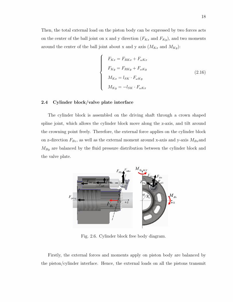
2.4 Cylinder block/valve plate interface

The cylinder block is assembled on the driving shaft through a crown shaped

spline joint, which allows the cylinder block move along the z-axis, and tilt around

the crowning point freely. Therefore, the external force applies on the cylinder block

on z-direction FBz, as well as the external moment around x-axis and y-axis MBxand

MBy are balanced by the fluid pressure distribution between the cylinder block and

the valve plate.

Fig. 2.6. Cylinder block free body diagram.

Firstly, the external forces and moments apply on piston body are balanced by

the piston/cylinder interface. Hence, the external loads on all the pistons transmit

19

through the piston/cylinder interfaces to the cylinder block body. The total forces

and moments from all pistons can be expressed using the global coordinate system:

FKBx =z∑i=1

(FRKxi + FωKxi)

FKBy =z∑i=1

(FRKyi + FωKyi)

MKBx =z∑i=1

((lSK −

HK

2+ sKi

)· FωKyi +

(sK −

HK

2

)FRKyi

)MKBy = −

z∑i=1

((lSK −

HK

2+ sKi

)· FωKxi +

(sK −

HK

2

)FRKxi

)(2.17)

Besides of the forces and moments from all pistons, cylinder block itself also subjects

to the displacement pressure force from all the displacement chambers.

For a single displacement chamber, the pressure force can be calculated from the

displacement pressure pDCi, piston diameter dK , and the kidney opening area Akidney.

FDBi = pDCi

(π · dK2

4− Akidney

)(2.18)

The pressure force induced moment then yields:MDBxi = pDCi ·

(ypiston i ·

π · dK2

4− ykidney i · Akidney

)MDByi = −pDCi ·

(xpiston i ·

π · dK2

4− xkidney i · Akidney

) (2.19)

Above equations to calculate the displacement chamber pressure force and moment

are correct only for the common axial piston machine design which fulfills two limi-

tations:

• The cylinder block running surface must be flat

• The pistons must be arranged parallelly to the shaft

Any axial piston machine design which does not fulfill these two limitations is out of

the scope of this dissertation.

20

The total force and moments due to the displacement chamber pressure yields:

FDB =z∑i=1

(pDCi ·

(π · dK2

4− Akidney

))MDBx =

z∑i=1

(pDCi ·

(ypiston i ·

π · dK2

4− ykidney i · Akidney

))MDBy =

z∑i=1

(−pDCi ·

(xpiston i ·

π · dK2

4− xkidney i · Akidney

)) (2.20)

At most of the operating conditions, the displacement pressure force dominates the

external force on z-direction. However, there are two more forces are necessary to be

considered when the unit runs under very low pressure.

The shaft spring that locates between the shaft and the cylinder block to pushes

the cylinder block toward the valve plate to keep the cylinder block at the desired

position when runs under very low pressure. This spring force Fspring acts as an

external force on the negative z-direction.

The force and moments from the viscous friction from all piston/cylinder interfaces

yields:

FTB =z∑i=1

(FTBi)

MTBx =z∑i=1

(ypiston i · FTBi)

MTBy =z∑i=1

(−xpiston i · FTBi)

(2.21)

The external forces applies on the cylinder block in x and y direction is balanced by

the reaction force from the shaft through the crown shape spline joint. Therefore,

moments about the global origin are generated when the tipping point of the spline

joint is not located exactly at the global origin.

The reaction force from the shaft follows the following equation:FSBx = −

z∑i=1

(FRKxi + FωKxi)

FSBy = −z∑i=1

(FRKyi + FωKyi)

(2.22)

21

The moment then can be derived using the location of the tipping point relative to

the global origin ztipping:MSBx = ztipping ·

z∑i=1

(FRKxi + FωKxi)

MSBy = −ztipping ·z∑i=1

(FRKyi + FωKyi)

(2.23)

The total external load that is balanced by the pressure distribution between the

cylinder block and the valve plate then can be expressed as:FB = FDB + Fspring + FTB

MBx = MKBx +MDBx +MTBx +MSBx

MBy = MKBy +MDBy +MTBy +MSBy

(2.24)

22

3. THE PROPOSED PISTON/CYLINDER INTERFACE

MODEL

The state-of-the-art piston/cylinder lubricating interface model is developed by Pelosi

[14] (cited as Pelosi’s model in this chapter). In this chapter, A multi-physics and

multi-domain piston/cylinder lubricating interface model is proposed which based on

Pelosi’s model with greatly improved accuracy and robustness. Comparing to Pelosi’s

base model, the proposed model advances at the following points:

• A backward difference squeeze term in the Reynolds equation.

• Improved FVM fluid domain discretion scheme.

• Physics-based boundaries for fluid film thickness.

• Advanced integrated solid body heat transfer model.

• Heat transfer model for compressible fluid.

3.1 Introduction to piston/cylinder interface modeling

Pelosi’s piston/cylinder interface structure and thermal interaction model solves

the fluid behavior in a discretized finite volume fluid domain. The two-dimensional

pressure distribution is solved using the Reynolds equation considering the gap sur-

face deformation, fluid properties, and piston kinematics and micromotion, and the

three-dimensional temperature distribution is solved using the energy equation con-

sidering the conduction, convection, and the viscous energy dissipation. A pressure

deformation model uses an off-line influence matrix method to solve the piston and

the cylinder block solid body deformation due to the fluid pressure. The fluid be-

havior, the pressure deformation, and the fluid properties influence each other in-

23

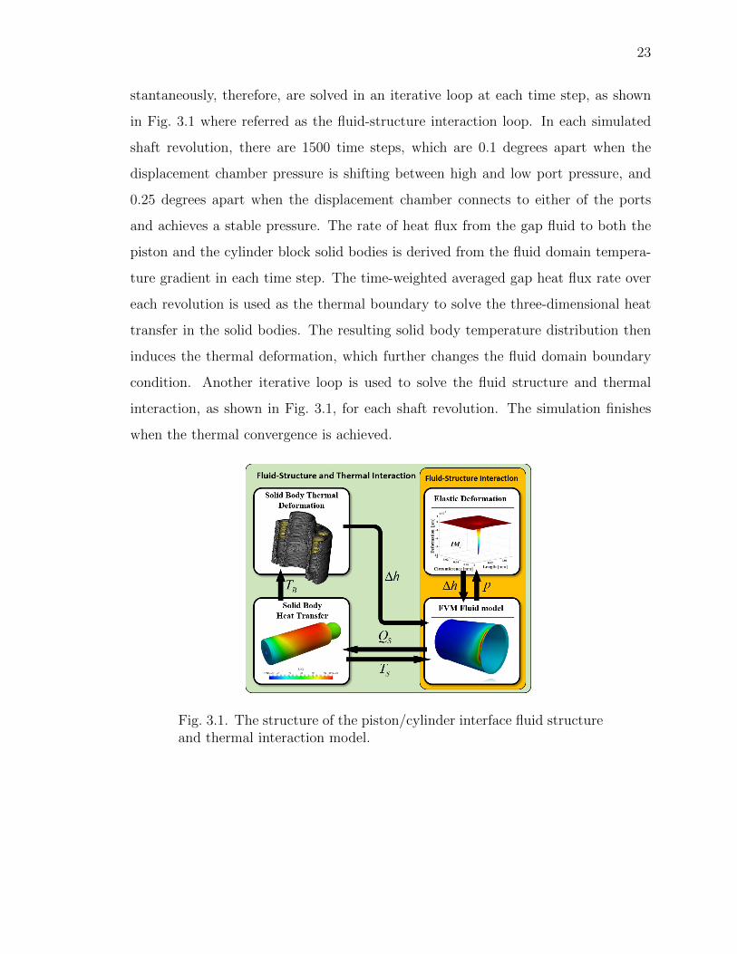
stantaneously, therefore, are solved in an iterative loop at each time step, as shown

in Fig. 3.1 where referred as the fluid-structure interaction loop. In each simulated

shaft revolution, there are 1500 time steps, which are 0.1 degrees apart when the

displacement chamber pressure is shifting between high and low port pressure, and

0.25 degrees apart when the displacement chamber connects to either of the ports

and achieves a stable pressure. The rate of heat flux from the gap fluid to both the

piston and the cylinder block solid bodies is derived from the fluid domain tempera-

ture gradient in each time step. The time-weighted averaged gap heat flux rate over

each revolution is used as the thermal boundary to solve the three-dimensional heat

transfer in the solid bodies. The resulting solid body temperature distribution then

induces the thermal deformation, which further changes the fluid domain boundary

condition. Another iterative loop is used to solve the fluid structure and thermal

interaction, as shown in Fig. 3.1, for each shaft revolution. The simulation finishes

when the thermal convergence is achieved.

Fig. 3.1. The structure of the piston/cylinder interface fluid structureand thermal interaction model.

24

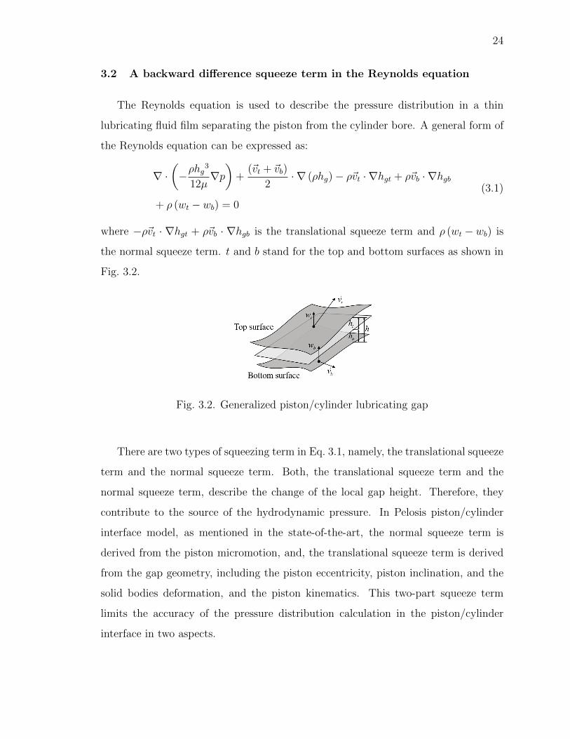
3.2 A backward difference squeeze term in the Reynolds equation

The Reynolds equation is used to describe the pressure distribution in a thin

lubricating fluid film separating the piston from the cylinder bore. A general form of

the Reynolds equation can be expressed as:

∇ ·(−ρhg

3

12µ∇p)

+(~vt + ~vb)

2· ∇ (ρhg)− ρ~vt · ∇hgt + ρ~vb · ∇hgb

+ ρ (wt − wb) = 0

(3.1)

where −ρ~vt · ∇hgt + ρ~vb · ∇hgb is the translational squeeze term and ρ (wt − wb) is

the normal squeeze term. t and b stand for the top and bottom surfaces as shown in

Fig. 3.2.

Fig. 3.2. Generalized piston/cylinder lubricating gap

There are two types of squeezing term in Eq. 3.1, namely, the translational squeeze

term and the normal squeeze term. Both, the translational squeeze term and the

normal squeeze term, describe the change of the local gap height. Therefore, they

contribute to the source of the hydrodynamic pressure. In Pelosis piston/cylinder

interface model, as mentioned in the state-of-the-art, the normal squeeze term is

derived from the piston micromotion, and, the translational squeeze term is derived

from the gap geometry, including the piston eccentricity, piston inclination, and the

solid bodies deformation, and the piston kinematics. This two-part squeeze term

limits the accuracy of the pressure distribution calculation in the piston/cylinder

interface in two aspects.

25

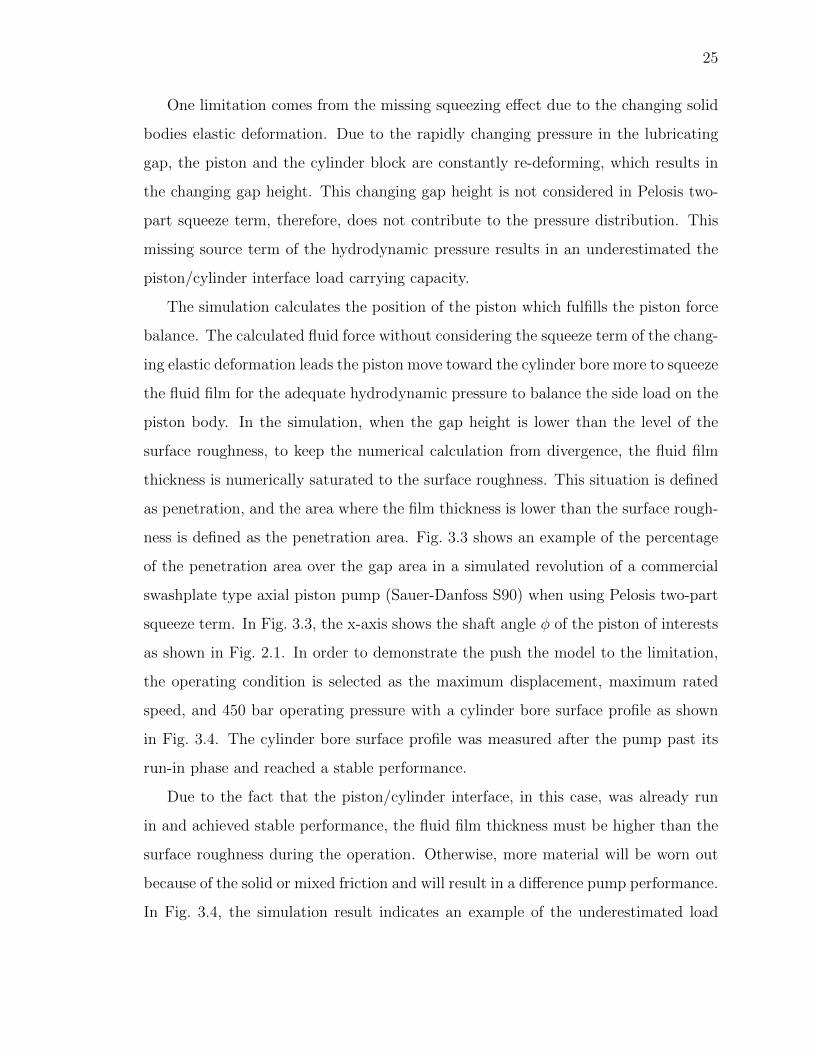
One limitation comes from the missing squeezing effect due to the changing solid

bodies elastic deformation. Due to the rapidly changing pressure in the lubricating

gap, the piston and the cylinder block are constantly re-deforming, which results in

the changing gap height. This changing gap height is not considered in Pelosis two-

part squeeze term, therefore, does not contribute to the pressure distribution. This

missing source term of the hydrodynamic pressure results in an underestimated the

piston/cylinder interface load carrying capacity.

The simulation calculates the position of the piston which fulfills the piston force

balance. The calculated fluid force without considering the squeeze term of the chang-

ing elastic deformation leads the piston move toward the cylinder bore more to squeeze

the fluid film for the adequate hydrodynamic pressure to balance the side load on the

piston body. In the simulation, when the gap height is lower than the level of the

surface roughness, to keep the numerical calculation from divergence, the fluid film

thickness is numerically saturated to the surface roughness. This situation is defined

as penetration, and the area where the film thickness is lower than the surface rough-

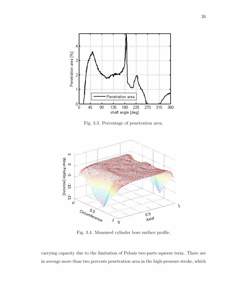
ness is defined as the penetration area. Fig. 3.3 shows an example of the percentage

of the penetration area over the gap area in a simulated revolution of a commercial

swashplate type axial piston pump (Sauer-Danfoss S90) when using Pelosis two-part

squeeze term. In Fig. 3.3, the x-axis shows the shaft angle φ of the piston of interests

as shown in Fig. 2.1. In order to demonstrate the push the model to the limitation,

the operating condition is selected as the maximum displacement, maximum rated

speed, and 450 bar operating pressure with a cylinder bore surface profile as shown

in Fig. 3.4. The cylinder bore surface profile was measured after the pump past its

run-in phase and reached a stable performance.

Due to the fact that the piston/cylinder interface, in this case, was already run

in and achieved stable performance, the fluid film thickness must be higher than the

surface roughness during the operation. Otherwise, more material will be worn out

because of the solid or mixed friction and will result in a difference pump performance.

In Fig. 3.4, the simulation result indicates an example of the underestimated load

26

Fig. 3.3. Percentage of penetration area.

Fig. 3.4. Measured cylinder bore surface profile.

carrying capacity due to the limitation of Pelosis two-parts squeeze term. There are

in average more than two percents penetration area in the high-pressure stroke, which

27

in this case is from 0 to 180 degrees shaft angle. In the low-pressure stroke, which

is from 180 to 360 degrees, there is around one percent of penetration. The surface

roughness, in this case, is measured at 0.1 microns.

One proposed solution is using a backward difference elasto-hydrodynamic (EHD)

squeeze term including the squeeze effect due to the changing elastic deformation to

the pressure distribution calculation. The Reynolds equation utilizing this backward

EHD squeeze term can be constructed as:

∇ ·(−ρhg

3

12µ∇p)

+(~vt + ~vb)

2· ∇ (ρhg)− ρ~vt · ∇hgt + ρ~vb · ∇hgb

+ρ (wt − wb) + ρ

(dhEHDdt

)= 0

(3.2)

where the backward difference EHD squeeze term is derived from:

dhgEHDdt

=hgEHD current − hgEHD previous

tcurrent − tprevious(3.3)

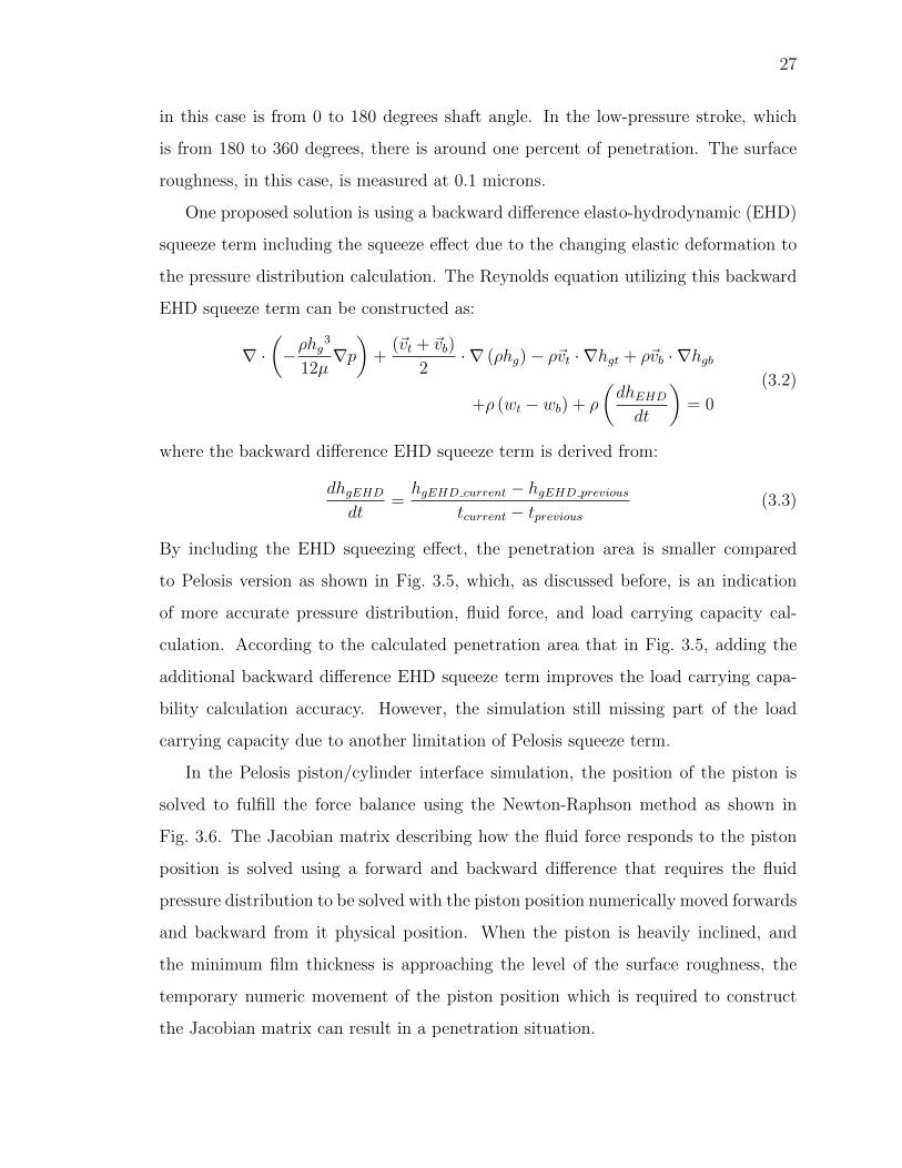
By including the EHD squeezing effect, the penetration area is smaller compared

to Pelosis version as shown in Fig. 3.5, which, as discussed before, is an indication

of more accurate pressure distribution, fluid force, and load carrying capacity cal-

culation. According to the calculated penetration area that in Fig. 3.5, adding the

additional backward difference EHD squeeze term improves the load carrying capa-

bility calculation accuracy. However, the simulation still missing part of the load

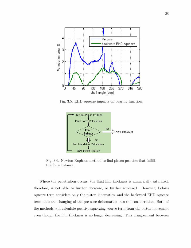
carrying capacity due to another limitation of Pelosis squeeze term.

In the Pelosis piston/cylinder interface simulation, the position of the piston is

solved to fulfill the force balance using the Newton-Raphson method as shown in

Fig. 3.6. The Jacobian matrix describing how the fluid force responds to the piston

position is solved using a forward and backward difference that requires the fluid

pressure distribution to be solved with the piston position numerically moved forwards

and backward from it physical position. When the piston is heavily inclined, and

the minimum film thickness is approaching the level of the surface roughness, the

temporary numeric movement of the piston position which is required to construct

the Jacobian matrix can result in a penetration situation.

28

Fig. 3.5. EHD squeeze impacts on bearing function.

Fig. 3.6. Newton-Raphson method to find piston position that fulfillsthe force balance.

Where the penetration occurs, the fluid film thickness is numerically saturated,

therefore, is not able to further decrease, or further squeezed. However, Pelosis

squeeze term considers only the piston kinematics, and the backward EHD squeeze

term adds the changing of the pressure deformation into the consideration. Both of

the methods still calculate positive squeezing source term from the piston movement

even though the film thickness is no longer decreasing. This disagreement between

29

the calculated film thickness and its changing rate results in an unrealistic pressure

distribution in the Jacobian matrix calculation, which then leads to an unrealistic

fluid force piston position response, and an unrealistic piston micromotion.

The proposed solution is a backward difference method to quantify the squeeze

term in the pressure distribution calculation from the current gap height, the previous

gap height, and the time difference between the current and the previous time step.

The Reynolds equation containing the proposed backward difference squeeze term is:

∇ ·(−ρh3g12µ∇p)

+(~vt + ~vb)

2· ∇ (ρhg)− ρ

(hgcurrent − hgprevioustcurrent − tprevious

)= 0 (3.4)

The proposed backward difference squeeze term covers all the physical and numerical

phenomena that impact the changing fluid film thickness completely since both the

current gap height and the previous gap height contain the rigid piston body position,

the pressure and the thermal deformation, and the film thickness numerical saturation

in the penetration area.

Fig. 3.7 shows the piston/cylinder interface simulation scheme using the proposed

backward difference squeeze term. The previous gap height as written as hgprevious

in Eq. 3.5 is updated after the fluid-structure interaction (FSI) loop and before the

force balance loop in each time step since the piston position is calculated using the

implicit Newton-Raphson method in the force balance loop.

As explained before, this penetration area is resulted from the unbalanced load,

which can be considered as the error between the calculated and the real load carrying

capacity. Fig. 3.8 shows the penetration area comparison between Pelosis squeeze

term, the backward EHD squeeze term, and the proposed backward difference squeeze

term. This comparison result demonstrates that the proposed backward difference

squeeze term significantly improves the piston/cylinder interface simulation accuracy,

especially in term of the load carrying capability calculation, from Pelosis baseline

simulation.

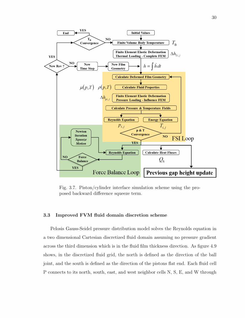
30

Fig. 3.7. Piston/cylinder interface simulation scheme using the pro-posed backward difference squeeze term.

3.3 Improved FVM fluid domain discretion scheme

Pelosis Gauss-Seidel pressure distribution model solves the Reynolds equation in

a two dimensional Cartesian discretized fluid domain assuming no pressure gradient

across the third dimension which is in the fluid film thickness direction. As figure 4.9

shows, in the discretized fluid grid, the north is defined as the direction of the ball

joint, and the south is defined as the direction of the pistons flat end. Each fluid cell

P connects to its north, south, east, and west neighbor cells N, S, E, and W through

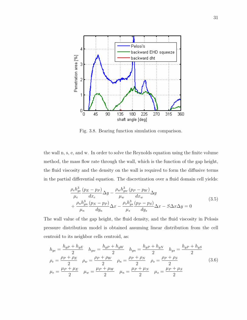
31

Fig. 3.8. Bearing function simulation comparison.

the wall n, s, e, and w. In order to solve the Reynolds equation using the finite volume

method, the mass flow rate through the wall, which is the function of the gap height,

the fluid viscosity and the density on the wall is required to form the diffusive terms

in the partial differential equation. The discretization over a fluid domain cell yields:

ρeh3ge

µe

(pE − pP )

dxe∆y −

ρwh3gw

µw

(pP − pW )

dxw∆y

+ρnh

3gn

µn

(pN − pP )

dyn∆x−

ρsh3gs

µs

(pP − pS)

dys∆x− S∆x∆y = 0

(3.5)

The wall value of the gap height, the fluid density, and the fluid viscosity in Pelosis

pressure distribution model is obtained assuming linear distribution from the cell

centroid to its neighbor cells centroid, as:

hge =hgP + hgE

2hgw =

hgP + hgW2

hgn =hgP + hgN

2hgs =

hgP + hgS2

ρe =ρP + ρE

2ρw =

ρP + ρW2

ρn =ρP + ρN

2ρs =

ρP + ρS2

µe =µP + µE

2µw =

µP + µW2

µn =µP + µN

2µs =

µP + µS2

(3.6)

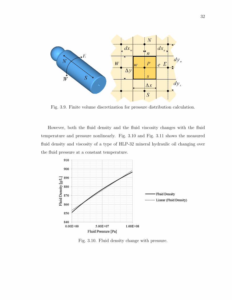
32

Fig. 3.9. Finite volume discretization for pressure distribution calculation.

However, both the fluid density and the fluid viscosity changes with the fluid

temperature and pressure nonlinearly. Fig. 3.10 and Fig. 3.11 shows the measured

fluid density and viscosity of a type of HLP-32 mineral hydraulic oil changing over

the fluid pressure at a constant temperature.

Fig. 3.10. Fluid density change with pressure.

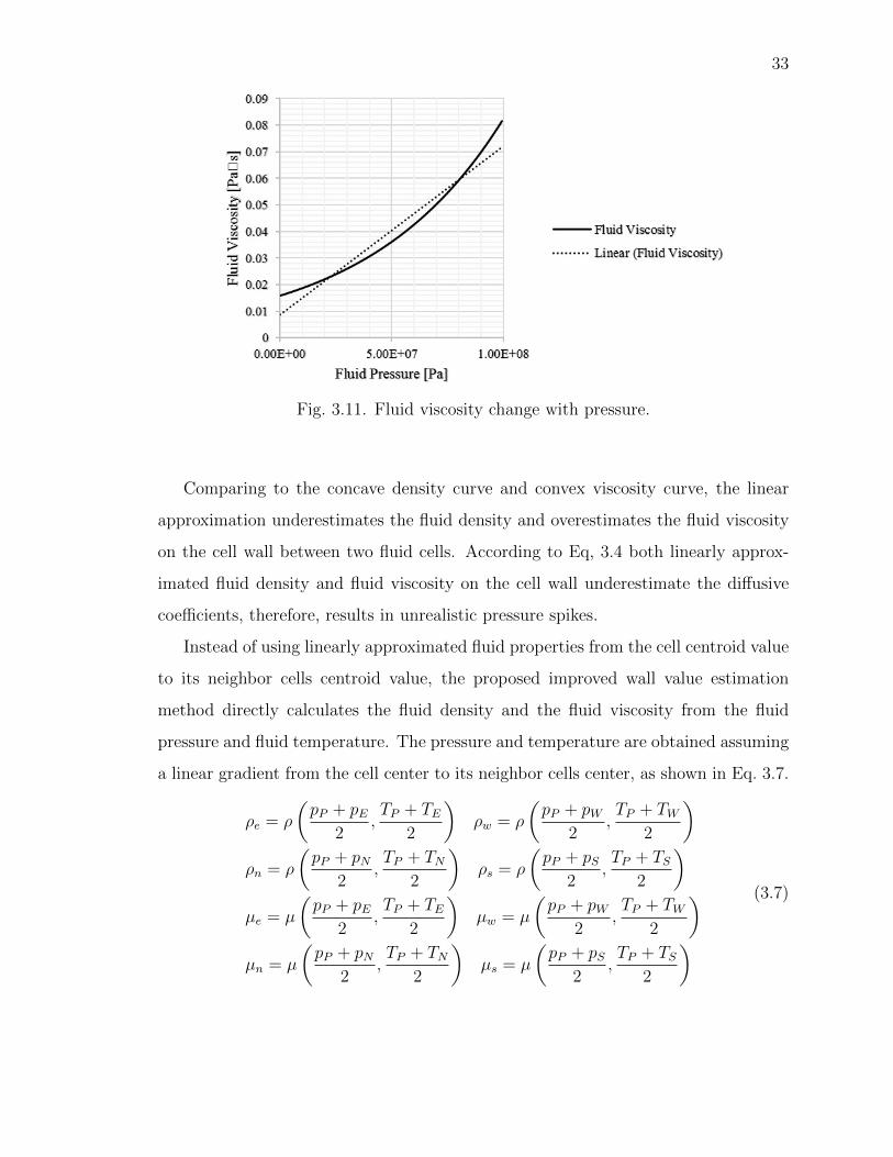
33

Fig. 3.11. Fluid viscosity change with pressure.

Comparing to the concave density curve and convex viscosity curve, the linear

approximation underestimates the fluid density and overestimates the fluid viscosity

on the cell wall between two fluid cells. According to Eq, 3.4 both linearly approx-

imated fluid density and fluid viscosity on the cell wall underestimate the diffusive

coefficients, therefore, results in unrealistic pressure spikes.

Instead of using linearly approximated fluid properties from the cell centroid value

to its neighbor cells centroid value, the proposed improved wall value estimation

method directly calculates the fluid density and the fluid viscosity from the fluid

pressure and fluid temperature. The pressure and temperature are obtained assuming

a linear gradient from the cell center to its neighbor cells center, as shown in Eq. 3.7.

ρe = ρ

(pP + pE

2,TP + TE

2

)ρw = ρ

(pP + pW

2,TP + TW

2

)ρn = ρ

(pP + pN

2,TP + TN

2

)ρs = ρ

(pP + pS

2,TP + TS

2

)µe = µ

(pP + pE

2,TP + TE

2

)µw = µ

(pP + pW

2,TP + TW

2

)µn = µ

(pP + pN

2,TP + TN

2

)µs = µ

(pP + pS

2,TP + TS

2

)(3.7)

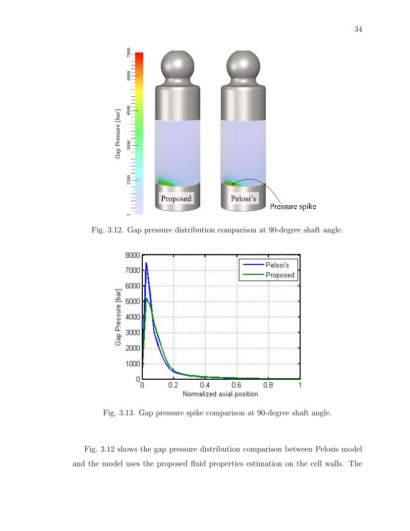
34

Fig. 3.12. Gap pressure distribution comparison at 90-degree shaft angle.

Fig. 3.13. Gap pressure spike comparison at 90-degree shaft angle.

Fig. 3.12 shows the gap pressure distribution comparison between Pelosis model

and the model uses the proposed fluid properties estimation on the cell walls. The

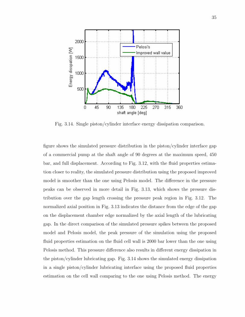
35

Fig. 3.14. Single piston/cylinder interface energy dissipation comparison.

figure shows the simulated pressure distribution in the piston/cylinder interface gap

of a commercial pump at the shaft angle of 90 degrees at the maximum speed, 450

bar, and full displacement. According to Fig. 3.12, with the fluid properties estima-

tion closer to reality, the simulated pressure distribution using the proposed improved

model is smoother than the one using Pelosis model. The difference in the pressure

peaks can be observed in more detail in Fig. 3.13, which shows the pressure dis-

tribution over the gap length crossing the pressure peak region in Fig. 3.12. The

normalized axial position in Fig. 3.13 indicates the distance from the edge of the gap

on the displacement chamber edge normalized by the axial length of the lubricating

gap. In the direct comparison of the simulated pressure spikes between the proposed

model and Pelosis model, the peak pressure of the simulation using the proposed

fluid properties estimation on the fluid cell wall is 2000 bar lower than the one using

Pelosis method. This pressure difference also results in different energy dissipation in

the piston/cylinder lubricating gap. Fig. 3.14 shows the simulated energy dissipation

in a single piston/cylinder lubricating interface using the proposed fluid properties

estimation on the cell wall comparing to the one using Pelosis method. The energy

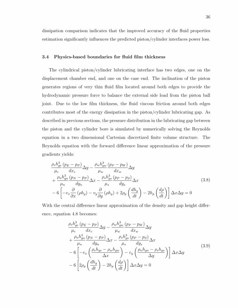
36

dissipation comparison indicates that the improved accuracy of the fluid properties

estimation significantly influences the predicted piston/cylinder interfaces power loss.

3.4 Physics-based boundaries for fluid film thickness

The cylindrical piston/cylinder lubricating interface has two edges, one on the

displacement chamber end, and one on the case end. The inclination of the piston

generates regions of very thin fluid film located around both edges to provide the

hydrodynamic pressure force to balance the external side load from the piston ball

joint. Due to the low film thickness, the fluid viscous friction around both edges

contributes most of the energy dissipation in the piston/cylinder lubricating gap. As

described in previous sections, the pressure distribution in the lubricating gap between

the piston and the cylinder bore is simulated by numerically solving the Reynolds

equation in a two dimensional Cartesian discretized finite volume structure. The

Reynolds equation with the forward difference linear approximation of the pressure

gradients yields:

ρeh3ge

µe

(pE − pP )

dxe∆y −

ρwh3gw

µw

(pP − pW )

dxw∆y

+ρnh

3gn

µn

(pN − pP )

dyn∆x−

ρsh3gs

µs

(pP − pS)

dys∆x

− 6

[−vx

∂

∂x(ρhg)− vy

∂

∂y(ρhg) + 2ρp

(dhgdt

)− 2hp

(dρ

dt

)]∆x∆y = 0

(3.8)

With the central difference linear approximation of the density and gap height differ-

ence, equation 4.8 becomes:

ρeh3ge

µe

(pE − pP )

dxe∆y −

ρwh3gw

µw

(pP − pW )

dxw∆y

+ρnh

3gn

µn

(pN − pP )

dyn∆x−

ρsh3gs

µs

(pP − pS)

dys∆x

− 6

[−vx

(ρehge − ρwhgw

∆x

)− vy

(ρnhgn − ρshgs

∆y

)]∆x∆y

− 6

[2ρp

(dhgdt

)− 2hp

(dρ

dt

)]∆x∆y = 0

(3.9)

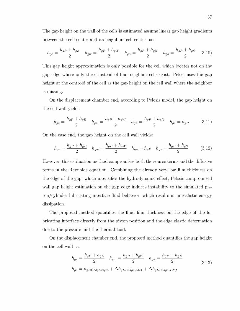
37

The gap height on the wall of the cells is estimated assume linear gap height gradients

between the cell center and its neighbors cell center, as:

hge =hgP + hgE

2hgw =

hgP + hgW2

hgn =hgP + hgN

2hgs =

hgP + hgS2

(3.10)

This gap height approximation is only possible for the cell which locates not on the

gap edge where only three instead of four neighbor cells exist. Pelosi uses the gap

height at the centroid of the cell as the gap height on the cell wall where the neighbor

is missing.

On the displacement chamber end, according to Pelosis model, the gap height on

the cell wall yields:

hge =hgP + hgE

2hgw =

hgP + hgW2

hgn =hgP + hgN

2hgs = hgP (3.11)

On the case end, the gap height on the cell wall yields:

hge =hgP + hgE

2hgw =

hgP + hgW2

hgn = hgP hgs =hgP + hgS

2(3.12)

However, this estimation method compromises both the source terms and the diffusive

terms in the Reynolds equation. Combining the already very low film thickness on

the edge of the gap, which intensifies the hydrodynamic effect, Pelosis compromised

wall gap height estimation on the gap edge induces instability to the simulated pis-

ton/cylinder lubricating interface fluid behavior, which results in unrealistic energy

dissipation.

The proposed method quantifies the fluid film thickness on the edge of the lu-

bricating interface directly from the piston position and the edge elastic deformation

due to the pressure and the thermal load.

On the displacement chamber end, the proposed method quantifies the gap height

on the cell wall as:

hge =hgP + hgE

2hgw =

hgP + hgW2

hgn =hgP + hgN

2

hgs = hgDCedge rigid + ∆hgDCedge pdef + ∆hgDCedge Tdef

(3.13)

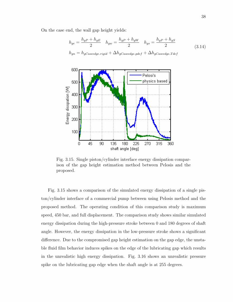
38

On the case end, the wall gap height yields:

hge =hgP + hgE

2hgw =

hgP + hgW2

hgs =hgP + hgS

2

hgn = hgCaseedge rigid + ∆hgCaseedge pdef + ∆hgCaseedge Tdef

(3.14)

Fig. 3.15. Single piston/cylinder interface energy dissipation compar-ison of the gap height estimation method between Pelosis and theproposed.

Fig. 3.15 shows a comparison of the simulated energy dissipation of a single pis-

ton/cylinder interface of a commercial pump between using Pelosis method and the

proposed method. The operating condition of this comparison study is maximum

speed, 450 bar, and full displacement. The comparison study shows similar simulated

energy dissipation during the high-pressure stroke between 0 and 180 degrees of shaft

angle. However, the energy dissipation in the low-pressure stroke shows a significant

difference. Due to the compromised gap height estimation on the gap edge, the unsta-

ble fluid film behavior induces spikes on the edge of the lubricating gap which results

in the unrealistic high energy dissipation. Fig. 3.16 shows an unrealistic pressure

spike on the lubricating gap edge when the shaft angle is at 255 degrees.

39

Note that there is no cylinder bore profile has been used in this comparison study

since the measured profile as Fig. 3.4 increase the film thickness around the gap edge.

The gap height on the edge is no longer critical when cylinder bore profile is applied,

therefore no significant difference between this two edge gap height methods.

Fig. 3.16. Pressure distribution comparison of the gap height estima-tion method between Pelosis and the proposed.

3.5 Advanced integrated solid body heat transfer model

The three-dimensional solid body heat transfer model for the piston/cylinder in-

terface mentioned in the previous chapter is based on the finite element discretization

of the solid bodies. The steady-state diffusive form of energy equation as shown in

Eq. 3.15 is used to determine the temperature distribution.

∇ · (κsolid∇T ) = 0 (3.15)

40

The temperature at each nodal position then solved in a linear system:

MPTP = qP

MBTB = qB

(3.16)

where TP and TB are the vectors of the temperature field of piston and cylinder block,

qP and qB are the vectors of the thermal boundaries on the piston and the cylinder

block solid bodies, and MP and MB are the matrices contain the conductivity between

each node. The conductivity matrices are constructed from the material properties

of the piston and the cylinder block solid bodies and the position of each node.

Unlike the simulation scheme of Pelosis model, which solves the temperature dis-

tribution in the piston and the cylinder block solid bodies separately, the proposed

advanced heat transfer model solves the dual-body temperature distribution in an

integrated linear system.

In this integrated linear system as shown in Eq. 3.17, there are two extra matrices

Mb2p and Mp2b contain the conductivity of the fluid film between the piston and the

cylinder block. MP 0

0 MB

+

Mb2p

Mp2b

TP

TB

=

qP

qB

(3.17)

In order to construct the matrix Mb2p, the relationship of the temperature at face

i of the piston running surface, the temperature at the face j on the cylinder bore

running surface, and the average heat flux between face i and face j in one shaft

revolution must be found first. The instantaneous piston/cylinder interface mesh

relative position is shown in Fig. 3.17.

For each single time step, the heat flux on piston face i can be determined by:

qi =κfluidhg(i,t)

(Tref − Ti) (3.18)

where hg(i,t) is the gap height and Tref is the cylinder bore surface temperature at

the reference location. As shown in figure 4.17, the reference location is defined as

the projection of face i on cylinder bore. Due to the relative motion of the piston,

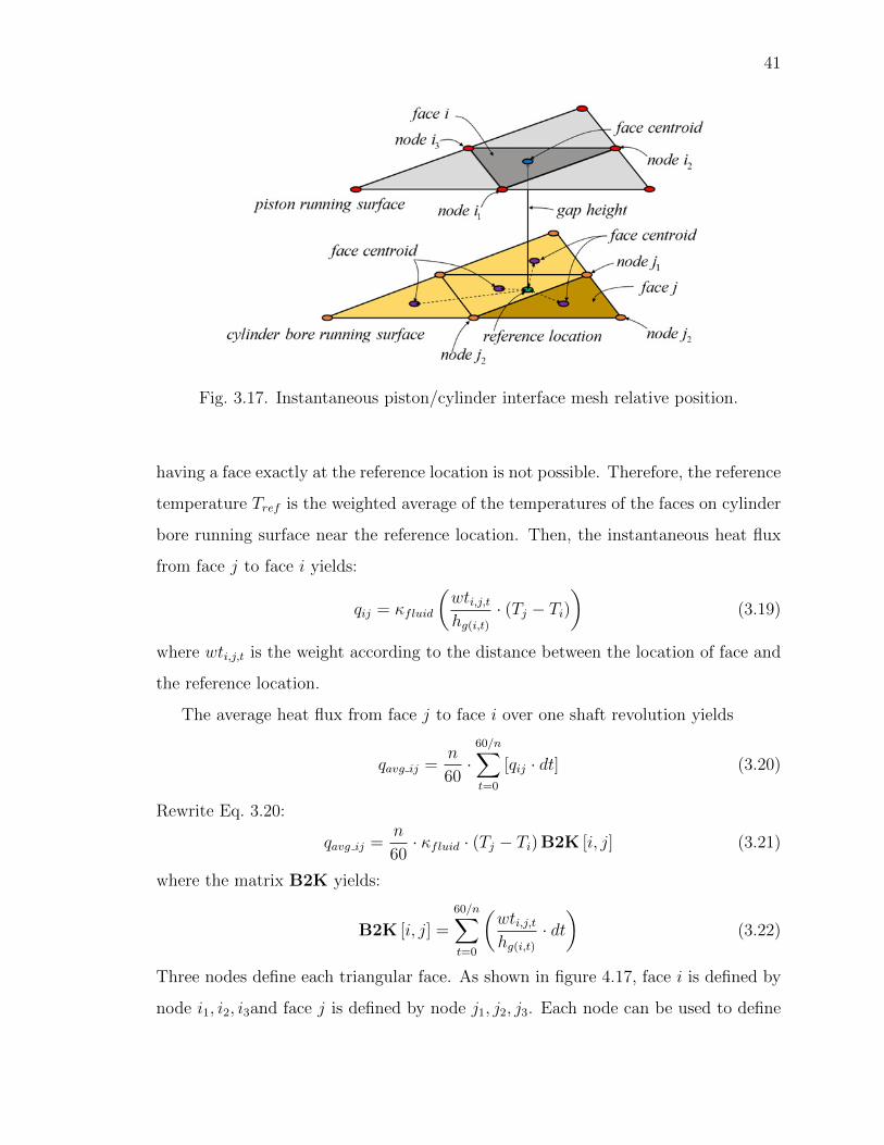
41

Fig. 3.17. Instantaneous piston/cylinder interface mesh relative position.

having a face exactly at the reference location is not possible. Therefore, the reference

temperature Tref is the weighted average of the temperatures of the faces on cylinder

bore running surface near the reference location. Then, the instantaneous heat flux

from face j to face i yields:

qij = κfluid

(wti,j,thg(i,t)

· (Tj − Ti))

(3.19)

where wti,j,t is the weight according to the distance between the location of face and

the reference location.

The average heat flux from face j to face i over one shaft revolution yields

qavg ij =n

60·60/n∑t=0

[qij · dt] (3.20)

Rewrite Eq. 3.20:

qavg ij =n

60· κfluid · (Tj − Ti) B2K [i, j] (3.21)

where the matrix B2K yields:

B2K [i, j] =

60/n∑t=0

(wti,j,thg(i,t)

· dt)

(3.22)

Three nodes define each triangular face. As shown in figure 4.17, face i is defined by

node i1, i2, i3and face j is defined by node j1, j2, j3. Each node can be used to define

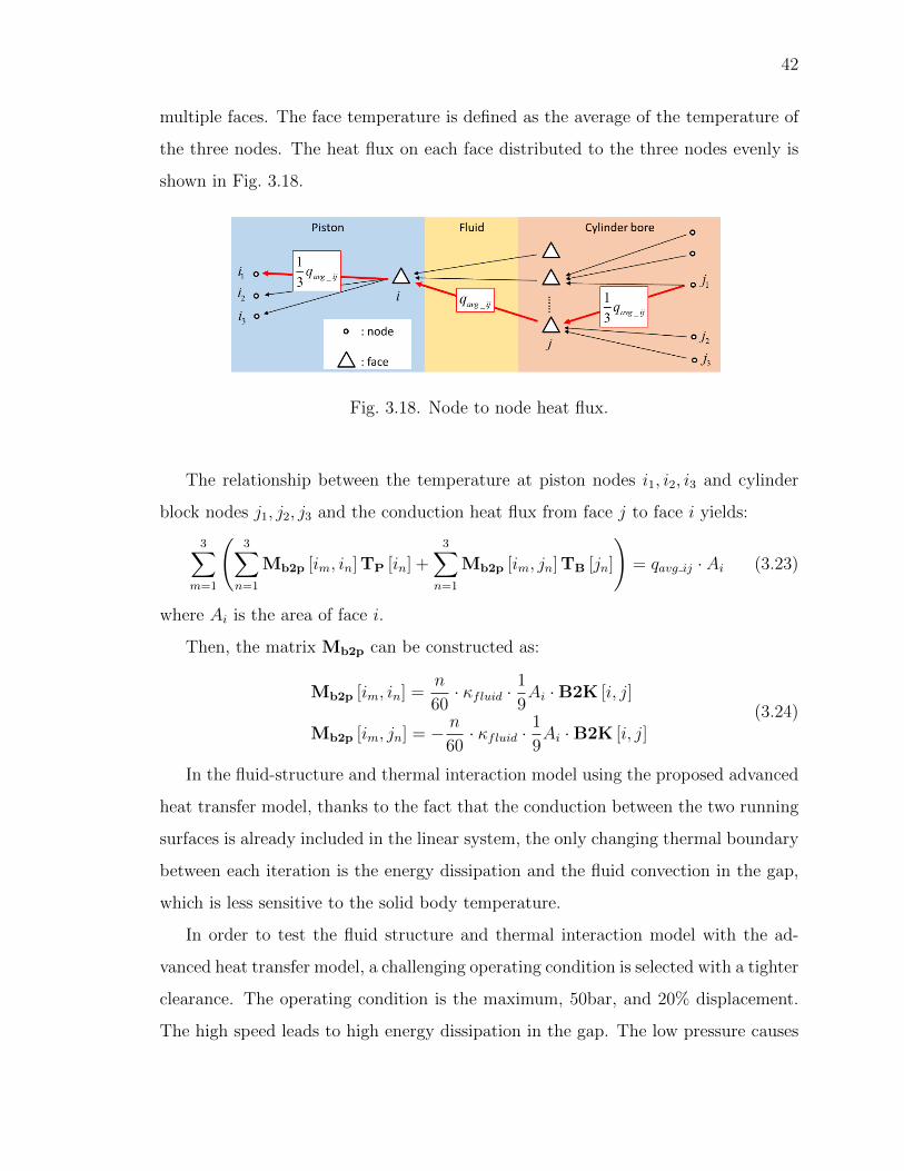
42

multiple faces. The face temperature is defined as the average of the temperature of

the three nodes. The heat flux on each face distributed to the three nodes evenly is

shown in Fig. 3.18.

Fig. 3.18. Node to node heat flux.

The relationship between the temperature at piston nodes i1, i2, i3 and cylinder

block nodes j1, j2, j3 and the conduction heat flux from face j to face i yields:

3∑m=1

(3∑

n=1

Mb2p [im, in] TP [in] +3∑

n=1

Mb2p [im, jn] TB [jn]

)= qavg ij · Ai (3.23)

where Ai is the area of face i.

Then, the matrix Mb2p can be constructed as:

Mb2p [im, in] =n

60· κfluid ·

1

9Ai ·B2K [i, j]

Mb2p [im, jn] = − n

60· κfluid ·

1

9Ai ·B2K [i, j]

(3.24)

In the fluid-structure and thermal interaction model using the proposed advanced

heat transfer model, thanks to the fact that the conduction between the two running

surfaces is already included in the linear system, the only changing thermal boundary

between each iteration is the energy dissipation and the fluid convection in the gap,

which is less sensitive to the solid body temperature.

In order to test the fluid structure and thermal interaction model with the ad-

vanced heat transfer model, a challenging operating condition is selected with a tighter

clearance. The operating condition is the maximum, 50bar, and 20% displacement.

The high speed leads to high energy dissipation in the gap. The low pressure causes

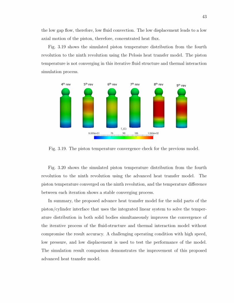
43

the low gap flow, therefore, low fluid convection. The low displacement leads to a low

axial motion of the piston, therefore, concentrated heat flux.

Fig. 3.19 shows the simulated piston temperature distribution from the fourth

revolution to the ninth revolution using the Pelosis heat transfer model. The piston

temperature is not converging in this iterative fluid structure and thermal interaction

simulation process.

Fig. 3.19. The piston temperature convergence check for the previous model.

Fig. 3.20 shows the simulated piston temperature distribution from the fourth

revolution to the ninth revolution using the advanced heat transfer model. The

piston temperature converged on the ninth revolution, and the temperature difference

between each iteration shows a stable converging process.

In summary, the proposed advance heat transfer model for the solid parts of the

piston/cylinder interface that uses the integrated linear system to solve the temper-

ature distribution in both solid bodies simultaneously improves the convergence of

the iterative process of the fluid-structure and thermal interaction model without

compromise the result accuracy. A challenging operating condition with high speed,

low pressure, and low displacement is used to test the performance of the model.

The simulation result comparison demonstrates the improvement of this proposed

advanced heat transfer model.

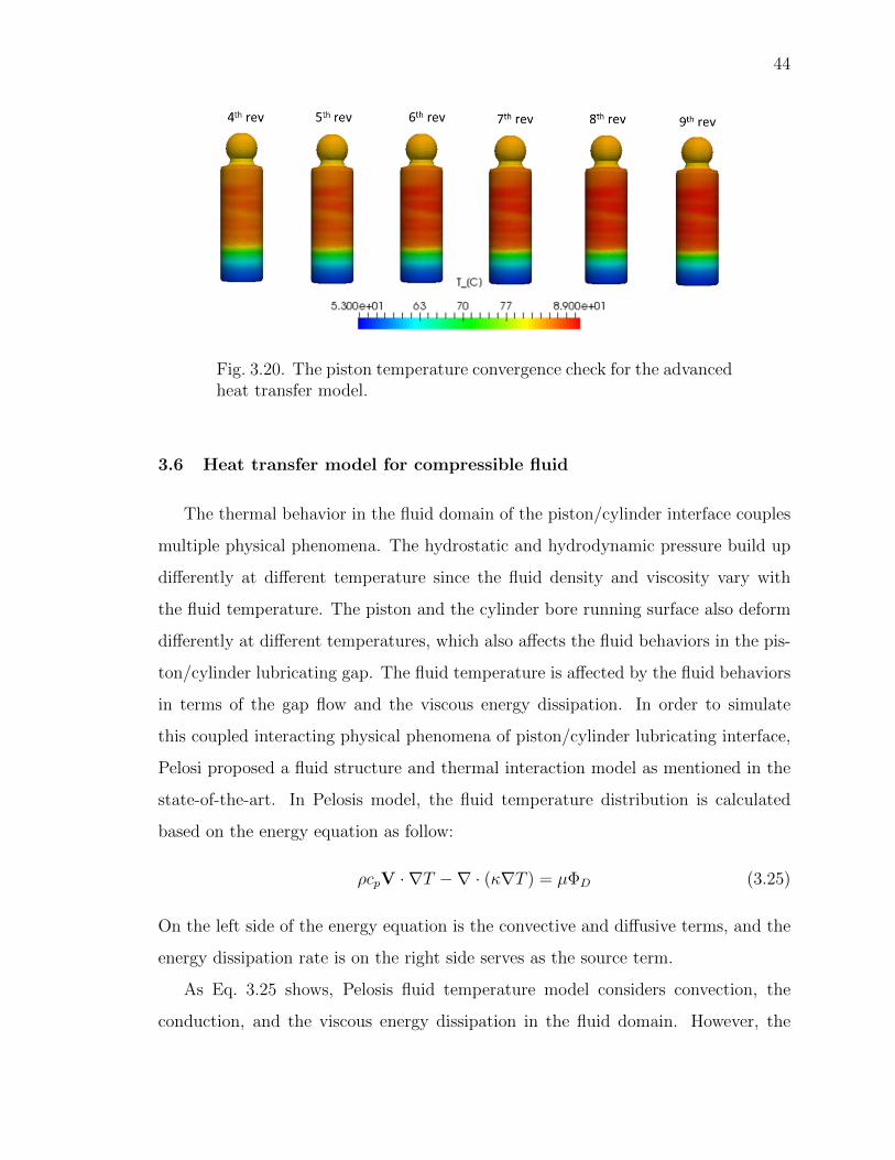
44

Fig. 3.20. The piston temperature convergence check for the advancedheat transfer model.

3.6 Heat transfer model for compressible fluid

The thermal behavior in the fluid domain of the piston/cylinder interface couples

multiple physical phenomena. The hydrostatic and hydrodynamic pressure build up

differently at different temperature since the fluid density and viscosity vary with

the fluid temperature. The piston and the cylinder bore running surface also deform

differently at different temperatures, which also affects the fluid behaviors in the pis-

ton/cylinder lubricating gap. The fluid temperature is affected by the fluid behaviors

in terms of the gap flow and the viscous energy dissipation. In order to simulate

this coupled interacting physical phenomena of piston/cylinder lubricating interface,

Pelosi proposed a fluid structure and thermal interaction model as mentioned in the

state-of-the-art. In Pelosis model, the fluid temperature distribution is calculated

based on the energy equation as follow:

ρcpV · ∇T −∇ · (κ∇T ) = µΦD (3.25)

On the left side of the energy equation is the convective and diffusive terms, and the

energy dissipation rate is on the right side serves as the source term.

As Eq. 3.25 shows, Pelosis fluid temperature model considers convection, the

conduction, and the viscous energy dissipation in the fluid domain. However, the

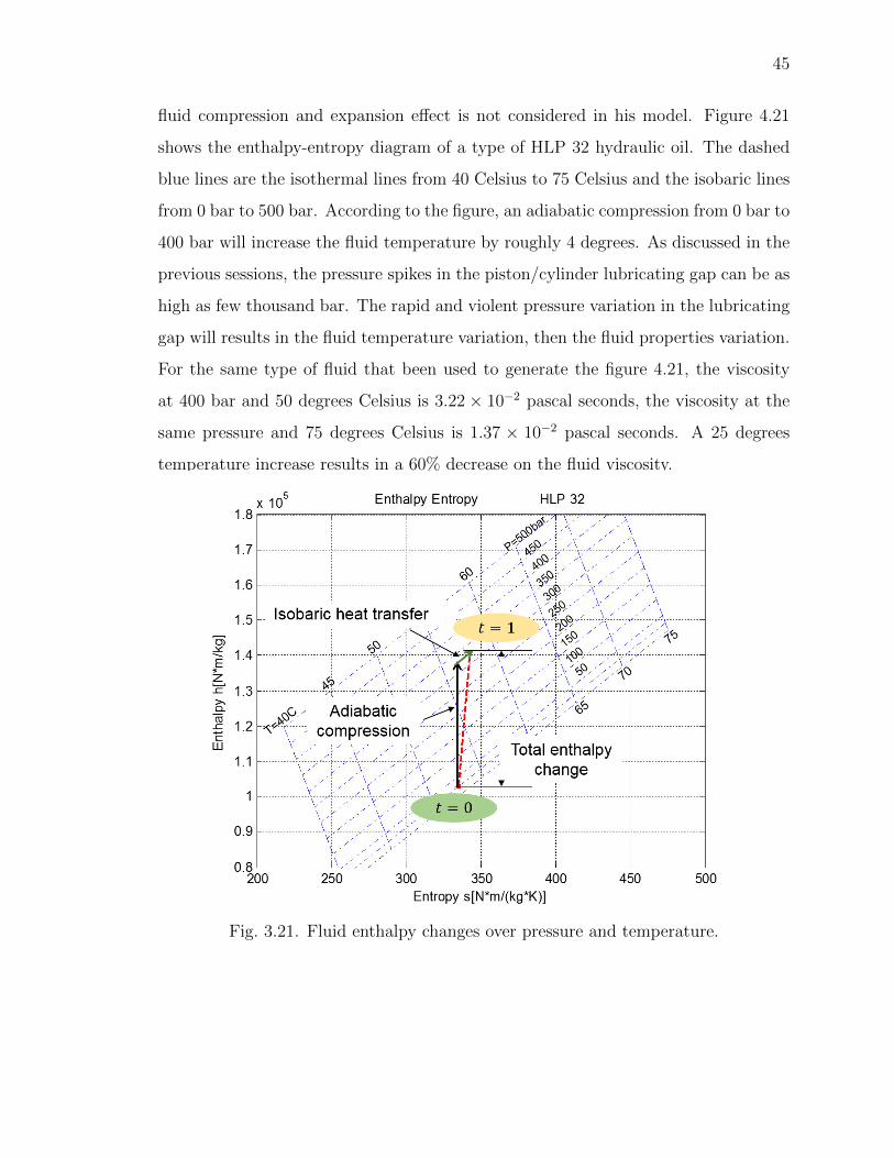
45

fluid compression and expansion effect is not considered in his model. Figure 4.21

shows the enthalpy-entropy diagram of a type of HLP 32 hydraulic oil. The dashed

blue lines are the isothermal lines from 40 Celsius to 75 Celsius and the isobaric lines

from 0 bar to 500 bar. According to the figure, an adiabatic compression from 0 bar to

400 bar will increase the fluid temperature by roughly 4 degrees. As discussed in the

previous sessions, the pressure spikes in the piston/cylinder lubricating gap can be as

high as few thousand bar. The rapid and violent pressure variation in the lubricating

gap will results in the fluid temperature variation, then the fluid properties variation.

For the same type of fluid that been used to generate the figure 4.21, the viscosity

at 400 bar and 50 degrees Celsius is 3.22 × 10−2 pascal seconds, the viscosity at the

same pressure and 75 degrees Celsius is 1.37 × 10−2 pascal seconds. A 25 degrees

temperature increase results in a 60% decrease on the fluid viscosity.

Fig. 3.21. Fluid enthalpy changes over pressure and temperature.

46

In order to capture the fluid temperature variation due to the compression and

expansion in the fluid domain temperature distribution model, enthalpy must be con-

sidered as the thermal property of the thermodynamic system. Burton [37] analyzed

the thermodynamics of a visco-elastic film under shear and compression. His study

combined the first and the second law of thermodynamics. Xu and Sadeghi [38]

reported their thermal EHL (elasto-hydrodynamic lubrication) analysis of circular

contacts with measured surface roughness. A three-dimensional time dependent non-

dimensional energy equation for the lubricating fluid was proposed which includes the

local temperature change with respect to time.

In the viscous fluid film of the piston/cylinder interface of the swashplate type

axial piston machine, the energy insert into the thermodynamic system not only as

work (pressure multiplied by the volume variation in common thermodynamic system)

but also as viscous energy dissipation. Also, the energy that pushes the viscous fluid

through the lubricating gap is partially from the volumetric variation as described in

the Reynolds equation and partially from the pressure differential across the gap. Due

to these facts, instead directly implement the enthalpy changing as in the common

thermodynamic system between time-steps in the simulation, the enthalpy of the

fluid in the control volume is calculated in a two-step process. As Fig. 3.21 shows,

the enthalpy changes from time step t = 0 to time step t = 1 is divided into an

adiabatic compression and an isobaric mass and heat transfer process. The governing

equation of the proposed thermal model then becomes:

H = H0 + ∆H|S + ∆H|p (3.26)

According to the differential of entropy:

ds =1

Tdh− 1

ρ · Tdp (3.27)

The isentropic enthalpy differential of pressure yields:

dh

dp

∣∣∣∣s

=1

ρ(3.28)

47

Then, the adiabatic enthalpy difference can be written as:

∆H|S = m0 ·p− p0ρ

(3.29)

The isobaric enthalpy difference in the control volume controlled by the convection,

conduction, and the energy dissipation:

∆H|p =

∫V

µΦDdV +

∫V

(ρV

dh

dp· ∇p

)dV

· dt+

∫A

(κ∇T − ρcpV · T − ρcTV · p) · dA

· dt(3.30)

The first term of the right side of Eq. 3.30 is the energy dissipation rate due to

the viscous shear in the fluid, the second term is the enthalpy difference due to the

pressure change of the flow, and the third term is the convection and the conduction.

In the third term:

cp =dh

dT

∣∣∣∣p

cT =dh

dp

∣∣∣∣T

(3.31)

As Fig. 3.21 shows, the isothermal line and the isobaric line are very linear. Therefore,

the two coefficients in Eq. 3.31 are assumed constant in the fluid domain temperature

distribution model.

In order to solve the heat transfer problem in the numerical simulation, the

fluid domain between the piston and the cylinder bore is discretized to a three-

dimensional finite volume grid as shown in Fig. 3.22(a) in Pelosis model. For each

three-dimensional finite volume as shown in Fig. 3.22(b), there are six faces labeled

t, b, w, e, n, and s separate the volume from its neighbors located at T, B, W, E, N,

and S. The mass in the control volume is changing due to the mass flow rate through

the faces w, e, n, and s. The fluid velocity on the gap height direction is assumed to

be zero. The temperature and the pressure in the control volume are token from the

centroid.

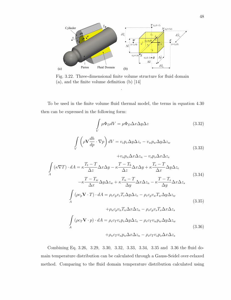
48

Fig. 3.22. Three-dimensional finite volume structure for fluid domain(a), and the finite volume definition (b) [14]

.

To be used in the finite volume fluid thermal model, the terms in equation 4.30

then can be expressed in the following form:∫V

µΦDdV = µΦD∆x∆y∆z (3.32)

∫V

(ρV

dh

dp· ∇p

)dV = vepe∆y∆ze − vwpw∆y∆zw

+vnpn∆x∆zn − vsps∆x∆zs

(3.33)

∫A

(κ∇T ) · dA = κTt − T

∆z∆x∆y − κT − Tb

∆z∆x∆y + κ

Te − T∆x

∆y∆ze

−κT − Tw∆x

∆y∆zw + κTn − T

∆y∆x∆zn − κ

T − Ts∆y

∆x∆zs

(3.34)

∫A

(ρcpV · T ) · dA = ρecpveTe∆y∆ze − ρecpvwTw∆y∆zw

+ρncpvnTn∆x∆zn − ρscpvsTs∆x∆zs

(3.35)

∫A

(ρcTV · p) · dA = ρecTvepe∆y∆ze − ρecTvwpw∆y∆zw

+ρncTvnpn∆x∆zn − ρscTvsps∆x∆zs

(3.36)

Combining Eq. 3.26, 3.29, 3.30, 3.32, 3.33, 3.34, 3.35 and 3.36 the fluid do-

main temperature distribution can be calculated through a Gauss-Seidel over-relaxed

method. Comparing to the fluid domain temperature distribution calculated using

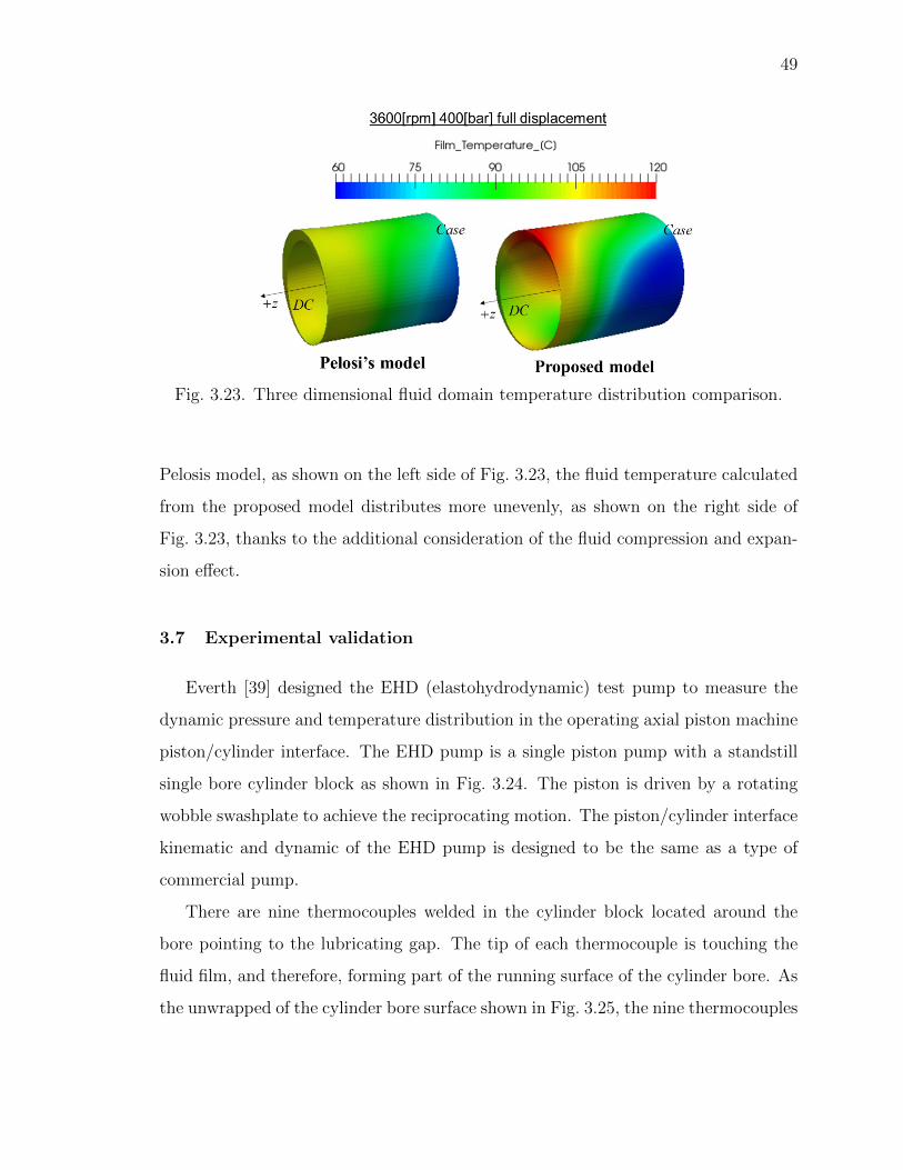
49

Fig. 3.23. Three dimensional fluid domain temperature distribution comparison.

Pelosis model, as shown on the left side of Fig. 3.23, the fluid temperature calculated

from the proposed model distributes more unevenly, as shown on the right side of

Fig. 3.23, thanks to the additional consideration of the fluid compression and expan-

sion effect.

3.7 Experimental validation

Everth [39] designed the EHD (elastohydrodynamic) test pump to measure the

dynamic pressure and temperature distribution in the operating axial piston machine

piston/cylinder interface. The EHD pump is a single piston pump with a standstill

single bore cylinder block as shown in Fig. 3.24. The piston is driven by a rotating

wobble swashplate to achieve the reciprocating motion. The piston/cylinder interface

kinematic and dynamic of the EHD pump is designed to be the same as a type of

commercial pump.

There are nine thermocouples welded in the cylinder block located around the

bore pointing to the lubricating gap. The tip of each thermocouple is touching the

fluid film, and therefore, forming part of the running surface of the cylinder bore. As

the unwrapped of the cylinder bore surface shown in Fig. 3.25, the nine thermocouples

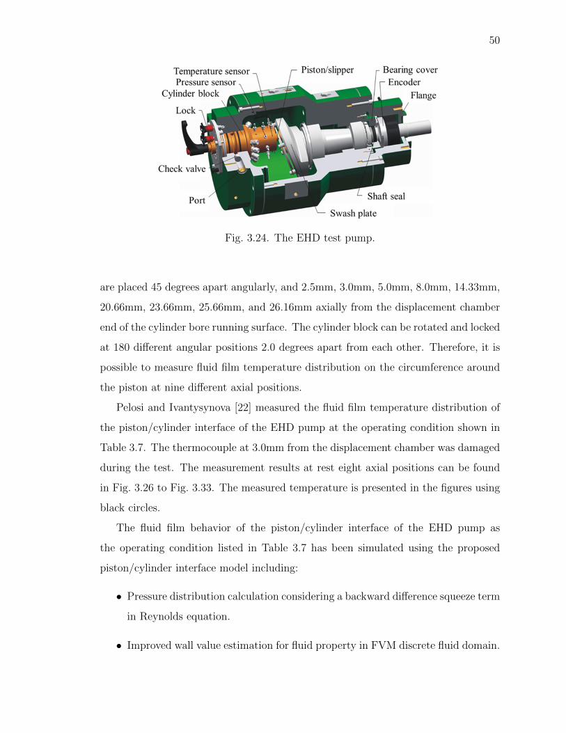
50

Fig. 3.24. The EHD test pump.

are placed 45 degrees apart angularly, and 2.5mm, 3.0mm, 5.0mm, 8.0mm, 14.33mm,

20.66mm, 23.66mm, 25.66mm, and 26.16mm axially from the displacement chamber

end of the cylinder bore running surface. The cylinder block can be rotated and locked

at 180 different angular positions 2.0 degrees apart from each other. Therefore, it is

possible to measure fluid film temperature distribution on the circumference around

the piston at nine different axial positions.

Pelosi and Ivantysynova [22] measured the fluid film temperature distribution of

the piston/cylinder interface of the EHD pump at the operating condition shown in

Table 3.7. The thermocouple at 3.0mm from the displacement chamber was damaged

during the test. The measurement results at rest eight axial positions can be found

in Fig. 3.26 to Fig. 3.33. The measured temperature is presented in the figures using

black circles.

The fluid film behavior of the piston/cylinder interface of the EHD pump as

the operating condition listed in Table 3.7 has been simulated using the proposed

piston/cylinder interface model including:

• Pressure distribution calculation considering a backward difference squeeze term

in Reynolds equation.

• Improved wall value estimation for fluid property in FVM discrete fluid domain.

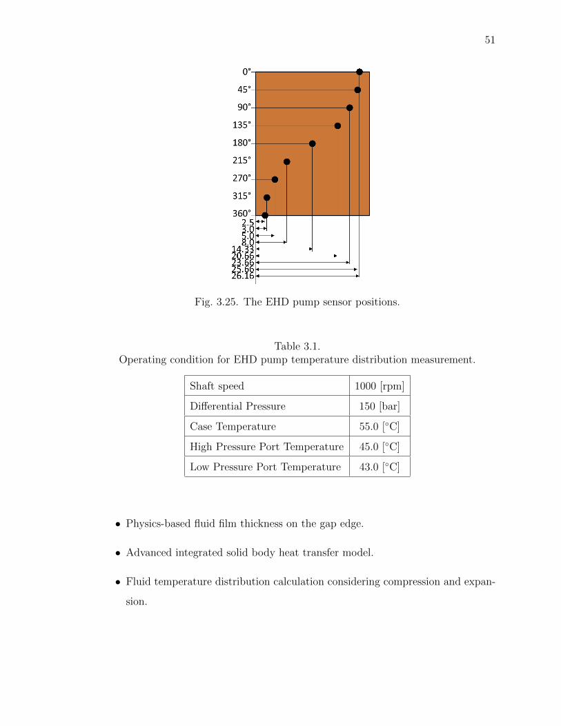
51

Fig. 3.25. The EHD pump sensor positions.

Table 3.1.Operating condition for EHD pump temperature distribution measurement.

Shaft speed 1000 [rpm]

Differential Pressure 150 [bar]

Case Temperature 55.0 [◦C]

High Pressure Port Temperature 45.0 [◦C]

Low Pressure Port Temperature 43.0 [◦C]

• Physics-based fluid film thickness on the gap edge.

• Advanced integrated solid body heat transfer model.

• Fluid temperature distribution calculation considering compression and expan-

sion.

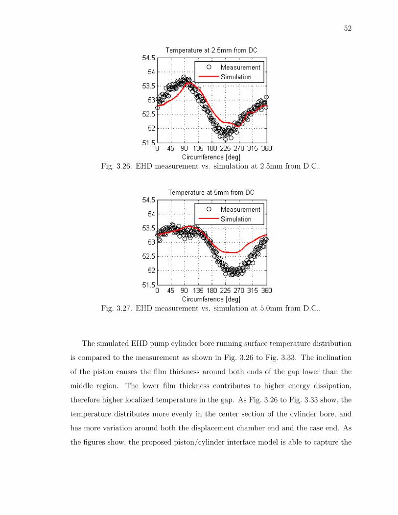
52

Fig. 3.26. EHD measurement vs. simulation at 2.5mm from D.C..


The simulated EHD pump cylinder bore running surface temperature distribution

is compared to the measurement as shown in Fig. 3.26 to Fig. 3.33. The inclination

of the piston causes the film thickness around both ends of the gap lower than the

middle region. The lower film thickness contributes to higher energy dissipation,

therefore higher localized temperature in the gap. As Fig. 3.26 to Fig. 3.33 show, the

temperature distributes more evenly in the center section of the cylinder bore, and

has more variation around both the displacement chamber end and the case end. As

the figures show, the proposed piston/cylinder interface model is able to capture the

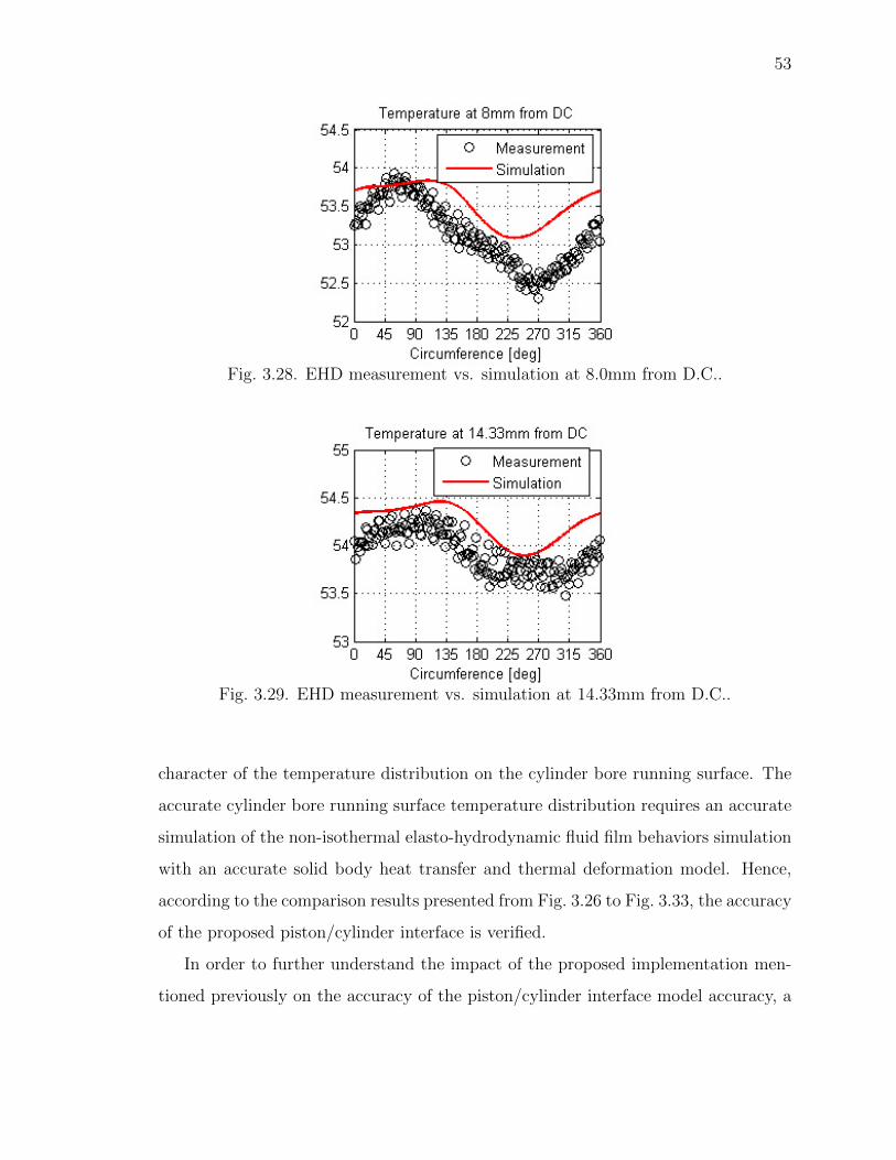
53



character of the temperature distribution on the cylinder bore running surface. The

accurate cylinder bore running surface temperature distribution requires an accurate

simulation of the non-isothermal elasto-hydrodynamic fluid film behaviors simulation

with an accurate solid body heat transfer and thermal deformation model. Hence,

according to the comparison results presented from Fig. 3.26 to Fig. 3.33, the accuracy

of the proposed piston/cylinder interface is verified.

In order to further understand the impact of the proposed implementation men-

tioned previously on the accuracy of the piston/cylinder interface model accuracy, a

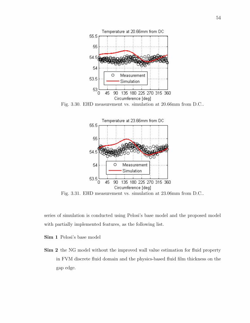
54



series of simulation is conducted using Pelosi’s base model and the proposed model

with partially implemented features, as the following list.

Sim 1 Pelosi’s base model

Sim 2 the NG model without the improved wall value estimation for fluid property

in FVM discrete fluid domain and the physics-based fluid film thickness on the

gap edge.

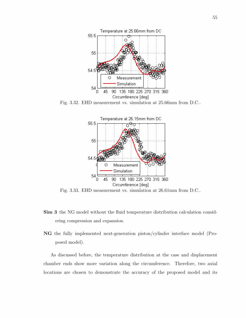
55



Sim 3 the NG model without the fluid temperature distribution calculation consid-

ering compression and expansion.

NG the fully implemented next-generation piston/cylinder interface model (Pro-

posed model).

As discussed before, the temperature distribution at the case and displacement

chamber ends show more variation along the circumference. Therefore, two axial

locations are chosen to demonstrate the accuracy of the proposed model and its

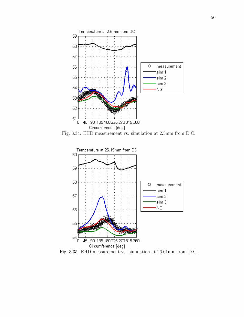
56



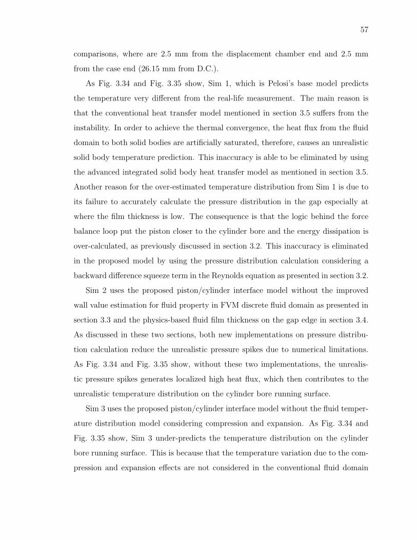
57

comparisons, where are 2.5 mm from the displacement chamber end and 2.5 mm

from the case end (26.15 mm from D.C.).

As Fig. 3.34 and Fig. 3.35 show, Sim 1, which is Pelosi’s base model predicts

the temperature very different from the real-life measurement. The main reason is

that the conventional heat transfer model mentioned in section 3.5 suffers from the

instability. In order to achieve the thermal convergence, the heat flux from the fluid

domain to both solid bodies are artificially saturated, therefore, causes an unrealistic

solid body temperature prediction. This inaccuracy is able to be eliminated by using

the advanced integrated solid body heat transfer model as mentioned in section 3.5.

Another reason for the over-estimated temperature distribution from Sim 1 is due to

its failure to accurately calculate the pressure distribution in the gap especially at

where the film thickness is low. The consequence is that the logic behind the force

balance loop put the piston closer to the cylinder bore and the energy dissipation is

over-calculated, as previously discussed in section 3.2. This inaccuracy is eliminated

in the proposed model by using the pressure distribution calculation considering a

backward difference squeeze term in the Reynolds equation as presented in section 3.2.

Sim 2 uses the proposed piston/cylinder interface model without the improved

wall value estimation for fluid property in FVM discrete fluid domain as presented in

section 3.3 and the physics-based fluid film thickness on the gap edge in section 3.4.

As discussed in these two sections, both new implementations on pressure distribu-

tion calculation reduce the unrealistic pressure spikes due to numerical limitations.

As Fig. 3.34 and Fig. 3.35 show, without these two implementations, the unrealis-

tic pressure spikes generates localized high heat flux, which then contributes to the

unrealistic temperature distribution on the cylinder bore running surface.

Sim 3 uses the proposed piston/cylinder interface model without the fluid temper-

ature distribution model considering compression and expansion. As Fig. 3.34 and

Fig. 3.35 show, Sim 3 under-predicts the temperature distribution on the cylinder

bore running surface. This is because that the temperature variation due to the com-

pression and expansion effects are not considered in the conventional fluid domain

58

heat transfer model. The proposed piston/cylinder interface model decomposes the

temperature variation in the fluid into two steps, an adiabatic pressure change process

and an isobaric heat generation and heat transfer process. As the comparison shows,

the proposed fluid temperature distribution model considering compression and ex-

pansion is able to improve the accuracy of the piston/cylinder interface simulation.

In summary, Fig. 3.26 to Fig. 3.33 present a comprehensive simulation verse mea-

surement comparison study. The proposed next-generation piston/cylinder interface

model is validated against the measurement for the temperature at 2880 different

locations on the cylinder bore running surface. Fig. 3.34 and Fig. 3.35 then demon-

strate how significant the influence of the implementations proposed in this chapter

on model accuracy.

3.8 Conclusion

In this chapter, a proposed next-generation piston/cylinder interface simulation

model is proposed, which advances over the previous generation model at the following

points:

• A backward difference squeeze term in the Reynolds equation.

• Improved FVM fluid domain discretion scheme.

• Physics-based boundaries for fluid film thickness.

• Advanced integrated solid body heat transfer model. [40]

• Heat transfer model for compressible fluid.. [41]

The physics behind each point and its implementation in the simulation is de-

scribed in detail in separate sections. The accuracy of the proposed model is verified

with the measurement by comparing the temperature distribution on the cylinder

bore running surface against the measured data obtained from a specially designed

elasto-hydrodynamic (EHD) pump. The significance of the implementation proposed

59

in this chapter is also demonstrated by comparing multiple partially implemented

model to the measurement.

60

4. THERMAL BOUNDARIES PREDICTION MODEL

For the simulations of existing pumps or motors, the essential port and case tem-

peratures are set based on the pump flow temperatures obtained from steady-state

measurements. However, in order to achieve the goal of understanding the perfor-

mance of a scaled swash plate type axial piston machine, the ability to conduct the

simulation studies without the support of the measurement is required. Therefore, a

tool that predicts the port and drain flow temperatures solely from the unit design is

demanded. A case flow temperature prediction model was proposed by Gronberg [42].

This model was further developed by Zecchi et al. [43]. A drawback of this model

is its sensitivity to user’s inputs, especially to the heat transfer area and the heat

transfer coefficients. The goal of this chapter is to develop a robust and accurate port

and case temperatures prediction model that can provide reliable thermal boundaries

to the three-dimensional multi-domain heat transfer model for the three lubricating

interfaces.

In this chapter, the scheme of the proposed thermal boundaries prediction model

as well as the governing physics are explained. The model is validated through a

comparison study between the simulated temperature and the measurement over

three hundred combinations of different units and different operation conditions.

4.1 Introduction to the thermal boundaries

The most recent simulation methodology for all three lubricating interfaces of

swash plate type axial piston machine (piston/cylinder, cylinder block/valve plate,

and slipper/swashplate) described in the previous chapters requires the temperatures

in the port volume and the case volume as the essential thermal boundaries. These

temperatures are not only used to calculate the three-dimensional temperature distri-

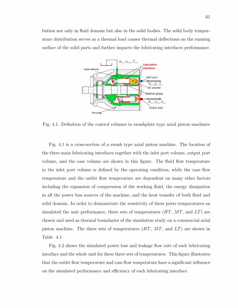
61

bution not only in fluid domain but also in the solid bodies. The solid body temper-

ature distribution serves as a thermal load causes thermal deflections on the running

surface of the solid parts and further impacts the lubricating interfaces performance.

Fig. 4.1. Definition of the control volumes in swashplate type axial piston machines

Fig. 4.1 is a cross-section of a swash type axial piston machine. The location of

the three main lubricating interfaces together with the inlet port volume, output port

volume, and the case volume are shown in this figure. The fluid flow temperature

in the inlet port volume is defined by the operating condition, while the case flow

temperature and the outlet flow temperature are dependent on many other factors

including the expansion of compression of the working fluid, the energy dissipation

in all the power loss sources of the machine, and the heat transfer of both fluid and

solid domain. In order to demonstrate the sensitivity of these ports temperatures on

simulated the unit performance, three sets of temperatures (HT , MT , and LT ) are

chosen and used as thermal boundaries of the simulation study on a commercial axial

piston machine. The three sets of temperatures (HT , MT , and LT ) are shown in

Table. 4.1.

Fig. 4.2 shows the simulated power loss and leakage flow rate of each lubricating

interface and the whole unit for these three sets of temperatures. This figure illustrates

that the outlet flow temperature and case flow temperature have a significant influence

on the simulated performance and efficiency of each lubricating interface.

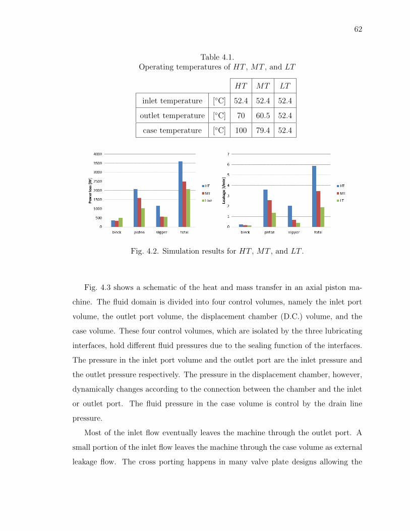
62

Table 4.1.Operating temperatures of HT , MT , and LT

HT MT LT

inlet temperature [◦C] 52.4 52.4 52.4

outlet temperature [◦C] 70 60.5 52.4

case temperature [◦C] 100 79.4 52.4

Fig. 4.2. Simulation results for HT , MT , and LT .

Fig. 4.3 shows a schematic of the heat and mass transfer in an axial piston ma-

chine. The fluid domain is divided into four control volumes, namely the inlet port

volume, the outlet port volume, the displacement chamber (D.C.) volume, and the

case volume. These four control volumes, which are isolated by the three lubricating

interfaces, hold different fluid pressures due to the sealing function of the interfaces.

The pressure in the inlet port volume and the outlet port are the inlet pressure and

the outlet pressure respectively. The pressure in the displacement chamber, however,

dynamically changes according to the connection between the chamber and the inlet

or outlet port. The fluid pressure in the case volume is control by the drain line

pressure.

Most of the inlet flow eventually leaves the machine through the outlet port. A

small portion of the inlet flow leaves the machine through the case volume as external

leakage flow. The cross porting happens in many valve plate designs allowing the

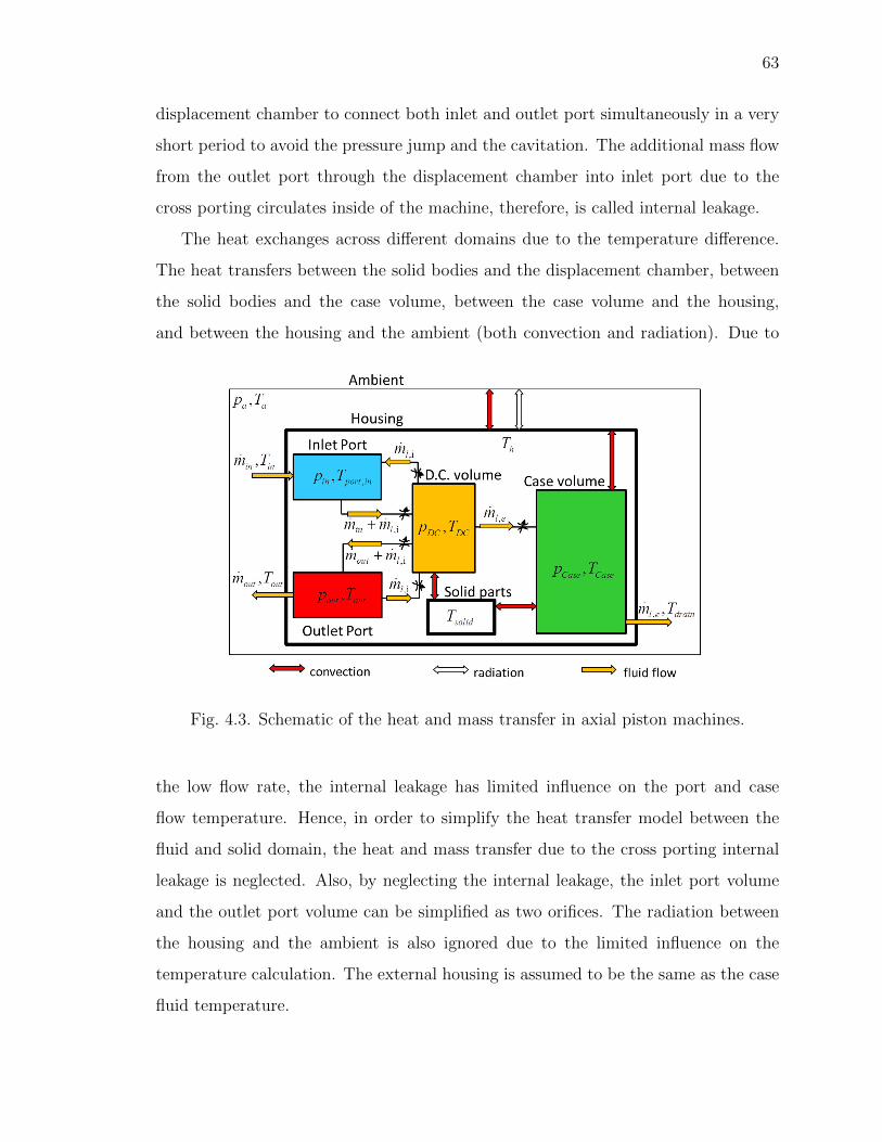
63

displacement chamber to connect both inlet and outlet port simultaneously in a very

short period to avoid the pressure jump and the cavitation. The additional mass flow

from the outlet port through the displacement chamber into inlet port due to the

cross porting circulates inside of the machine, therefore, is called internal leakage.

The heat exchanges across different domains due to the temperature difference.

The heat transfers between the solid bodies and the displacement chamber, between

the solid bodies and the case volume, between the case volume and the housing,

and between the housing and the ambient (both convection and radiation). Due to

Fig. 4.3. Schematic of the heat and mass transfer in axial piston machines.

the low flow rate, the internal leakage has limited influence on the port and case

flow temperature. Hence, in order to simplify the heat transfer model between the

fluid and solid domain, the heat and mass transfer due to the cross porting internal

leakage is neglected. Also, by neglecting the internal leakage, the inlet port volume

and the outlet port volume can be simplified as two orifices. The radiation between

the housing and the ambient is also ignored due to the limited influence on the

temperature calculation. The external housing is assumed to be the same as the case

fluid temperature.

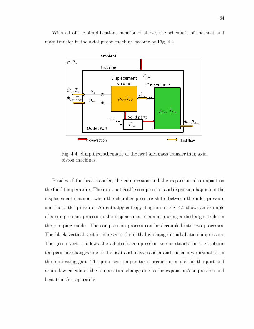
64

With all of the simplifications mentioned above, the schematic of the heat and

mass transfer in the axial piston machine become as Fig. 4.4.

Fig. 4.4. Simplified schematic of the heat and mass transfer in in axialpiston machines.

Besides of the heat transfer, the compression and the expansion also impact on

the fluid temperature. The most noticeable compression and expansion happen in the

displacement chamber when the chamber pressure shifts between the inlet pressure

and the outlet pressure. An enthalpy-entropy diagram in Fig. 4.5 shows an example

of a compression process in the displacement chamber during a discharge stroke in

the pumping mode. The compression process can be decoupled into two processes.

The black vertical vector represents the enthalpy change in adiabatic compression.

The green vector follows the adiabatic compression vector stands for the isobaric

temperature changes due to the heat and mass transfer and the energy dissipation in

the lubricating gap. The proposed temperatures prediction model for the port and

drain flow calculates the temperature change due to the expansion/compression and

heat transfer separately.

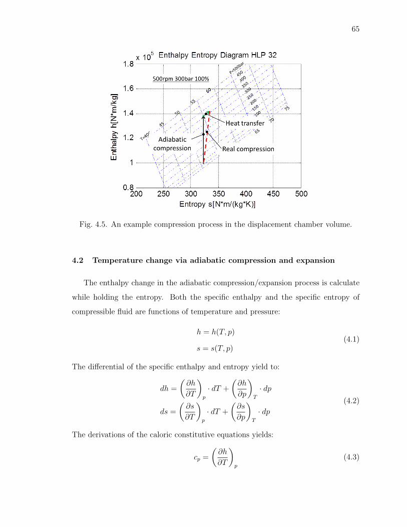
65

Fig. 4.5. An example compression process in the displacement chamber volume.

4.2 Temperature change via adiabatic compression and expansion

The enthalpy change in the adiabatic compression/expansion process is calculate

while holding the entropy. Both the specific enthalpy and the specific entropy of

compressible fluid are functions of temperature and pressure:

h = h(T, p)

s = s(T, p)(4.1)

The differential of the specific enthalpy and entropy yield to:

dh =

(∂h

∂T

)p

· dT +

(∂h

∂p

)T

· dp

ds =

(∂s

∂T

)p

· dT +

(∂s

∂p

)T

· dp(4.2)

The derivations of the caloric constitutive equations yields:

cp =

(∂h

∂T

)p

(4.3)

66

Using the Maxwell relation:

ds =

(∂s

∂T

)p

· dT −(∂vfluid∂T

)p

· dp (4.4)

where vfluid is the specific volume of the fluid. Substituting dh and ds into ds =

T · ds+ vfluid · dp[(∂h

∂p

)T

+ T

(∂vfluid∂T

)p

− vfluid

]dp =

[T

(∂s

∂T

)p

−(∂h

∂T

)p

]dT (4.5)

At constant temperature:[(∂h

∂p

)T

+ T

(∂v

∂T

)p

− vfluid

]dp = 0(

∂h

∂p

)T

= vfluid − T(∂vfluid∂T

)p

(4.6)

At constant pressure:

0 =

[T

(∂s

∂T

)p

−(∂h

∂T

)p

]dT(

∂s

∂T

)p

=1

T

(∂h

∂T

)p

=1

Tcp

(4.7)

Applied Eq. 4.3 and Eq. 4.6 to Eq. 4.2:

dh = cp · dT +

(vfluid − T ·

(∂vfluid∂T

)p

)· dp (4.8)

Applied Eq. 4.7 to Eq. 4.4:

ds = cp ·dT

T−(∂vfluid∂T

)p

· dp (4.9)

Integrating Eq. 4.8 and Eq. 4.9 at Toandpo:

h = ho (To) +

T∫To

cp · dT +

p∫p0

v · dp−p∫

p0

T ·(∂vfluid∂T

)p

· dp

s = so (To) +

T∫To

cpT· dT −

p∫p0

(∂vfluid∂T

)p

· dp

(4.10)

67

Based on the adiabatic compression assumption, the entropy of the fluid before and

after the compression or the expansion is the same:

s1 = s2

T1∫To

cpT· dT −

p1∫p0

(∂vfluid∂T

)p

· dp =

T2∫To

cpT· dT −

p2∫p0

(∂vfluid∂T

)p

· dp(4.11)

The temperature of the fluid after the adiabatic compression or expansion in both

displacement and case volume Tadia DC and Tadia Case can be solved by using Eq. 4.11.

4.3 Temperature change via heat transfer

The heat transfer process in the axial piston machine presented in Fig. 4.4 is fur-

ther simplified into a symbolized three-volume model which includes a displacement

chamber volume, a solid parts volume, and a case volume as shown in Fig. 4.6. The

energy dissipation rate due to the viscous friction is retro-proportional to the gap

height. The majority of the viscous friction power dissipates into heat in the gap area

where the minimum film thickness occurs. Because of the low film thickness, this

dissipated heat transfers into the solid bodies directly as conduction instead of into

case volume through convection. Therefore, the total power loss of the axial piston

machine is considered as a heat source which provides a rate of heat flux directly

into the solid parts volume. The power leaves the unit through two paths: either

transfers into the displacement chamber, then leaves the unit with the outlet flow;

or transfers in the case volume then leaves the machine with the drain flow or the

natural convection of the external housing surface.

The energy dissipation in the lubricating interfaces leaves solid parts in two ways:

qloss = qs DC + qs Case (4.12)

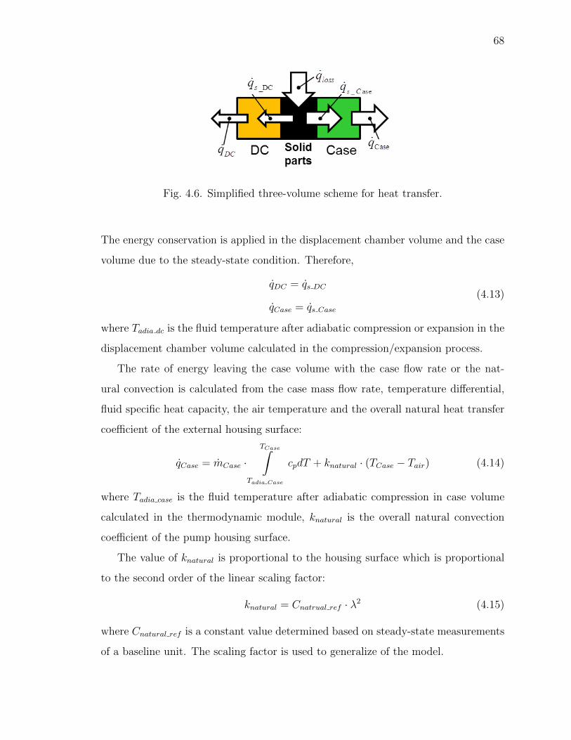
68

Fig. 4.6. Simplified three-volume scheme for heat transfer.

The energy conservation is applied in the displacement chamber volume and the case

volume due to the steady-state condition. Therefore,

qDC = qs DC

qCase = qs Case

(4.13)

where Tadia dc is the fluid temperature after adiabatic compression or expansion in the

displacement chamber volume calculated in the compression/expansion process.

The rate of energy leaving the case volume with the case flow rate or the nat-

ural convection is calculated from the case mass flow rate, temperature differential,

fluid specific heat capacity, the air temperature and the overall natural heat transfer

coefficient of the external housing surface:

qCase = mCase ·TCase∫

Tadia Case

cpdT + knatural · (TCase − Tair) (4.14)

where Tadia case is the fluid temperature after adiabatic compression in case volume

calculated in the thermodynamic module, knatural is the overall natural convection

coefficient of the pump housing surface.

The value of knatural is proportional to the housing surface which is proportional

to the second order of the linear scaling factor:

knatural = Cnatrual ref · λ2 (4.15)

where Cnatural ref is a constant value determined based on steady-state measurements

of a baseline unit. The scaling factor is used to generalize of the model.

69

The linear scaling factor can be obtained as:

λ = 3

√Vi

Vi baseline(4.16)

where Vi is the displacement volume of the pump or motor under investigation.

The rate of energy from solid parts to both the displacement chamber volume and

the case volume can be calculated as:

qs DC = kDC · (Tsolid − TDC)

qs Case = kCase · (Tsolid − TCase)(4.17)

where kDC and kCase are the overall heat transfer coefficients of the displacement

chamber surface and the case volume surface, TDC is the temperature in the displace-

ment chamber which approximately equals to the average of the inlet flow temperature

and the outlet flow temperature.

The value of kDC is a function of outlet flow rate and the linear scaling factor:

kDC =

(Qout

λ

)0.4

· λ2 · CDC ref (4.18)

where CDC ref is a constant value determined based on the steady state measurement,

the scaling reference, and fluid properties. The term Qout

λscales the overall heat

transfer coefficient with Reynolds number; the order value 0.4 is found that match

the measurements the best, and the term λ2 scales the overall heat transfer coefficient

with the heat transfer surface area.

The value of kcase is a function of the pump speed, the leakage flow rate correction

factor (lcf) and the linear scaling factor:

kCase =(n · λ2 · lcf

)0.4 · λ2 · CCase ref (4.19)

where CCase ref is a constant value determined based on the steady state measurement,

the scaling reference, and fluid property. The term n · λ2 · lcf scales the overall heat

transfer coefficient with Reynolds number; the order value 0.4 is found that match

the measurements the best, and the term λ2 scales the overall heat transfer coefficient

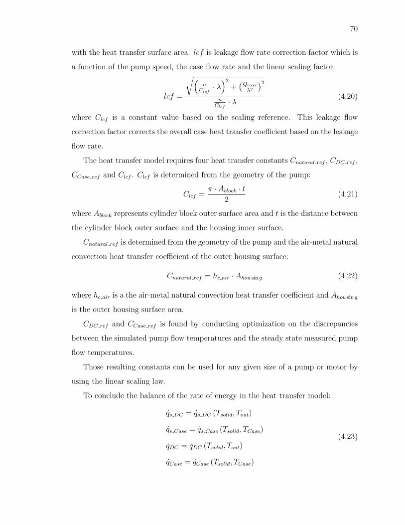
70

with the heat transfer surface area. lcf is leakage flow rate correction factor which is

a function of the pump speed, the case flow rate and the linear scaling factor:

lcf =

√(n

Clcf· λ)2

+(Qcase

λ2

)2n

Clcf· λ

(4.20)

where Clcf is a constant value based on the scaling reference. This leakage flow

correction factor corrects the overall case heat transfer coefficient based on the leakage

flow rate.

The heat transfer model requires four heat transfer constants Cnatural ref , CDC ref ,

CCase ref and Clcf . Clcf is determined from the geometry of the pump:

Clcf =π · Ablock · t

2(4.21)

where Ablock represents cylinder block outer surface area and t is the distance between

the cylinder block outer surface and the housing inner surface.

Cnatural ref is determined from the geometry of the pump and the air-metal natural

convection heat transfer coefficient of the outer housing surface:

Cnatural ref = hc air · Ahou sin g (4.22)

where hc air is a the air-metal natural convection heat transfer coefficient and Ahou sin g

is the outer housing surface area.

CDC ref and CCase ref is found by conducting optimization on the discrepancies

between the simulated pump flow temperatures and the steady state measured pump

flow temperatures.

Those resulting constants can be used for any given size of a pump or motor by

using the linear scaling law.

To conclude the balance of the rate of energy in the heat transfer model:

qs DC = qs DC (Tsolid, Tout)

qs Case = qs Case (Tsolid, TCase)

qDC = qDC (Tsolid, Tout)

qCase = qCase (Tsolid, TCase)

(4.23)

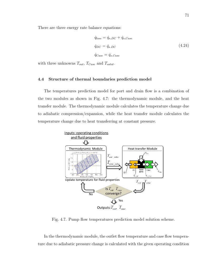
71

There are three energy rate balance equations:

qloss = qs DC + qs Case

qDC = qs DC

qCase = qs Case

(4.24)

with three unknowns Tout, TCase and Tsolid.

4.4 Structure of thermal boundaries prediction model

The temperatures prediction model for port and drain flow is a combination of

the two modules as shown in Fig. 4.7: the thermodynamic module, and the heat

transfer module. The thermodynamic module calculates the temperature change due

to adiabatic compression/expansion, while the heat transfer module calculates the

temperature change due to heat transferring at constant pressure.

Fig. 4.7. Pump flow temperatures prediction model solution scheme.

In the thermodynamic module, the outlet flow temperature and case flow tempera-

ture due to adiabatic pressure change is calculated with the given operating condition

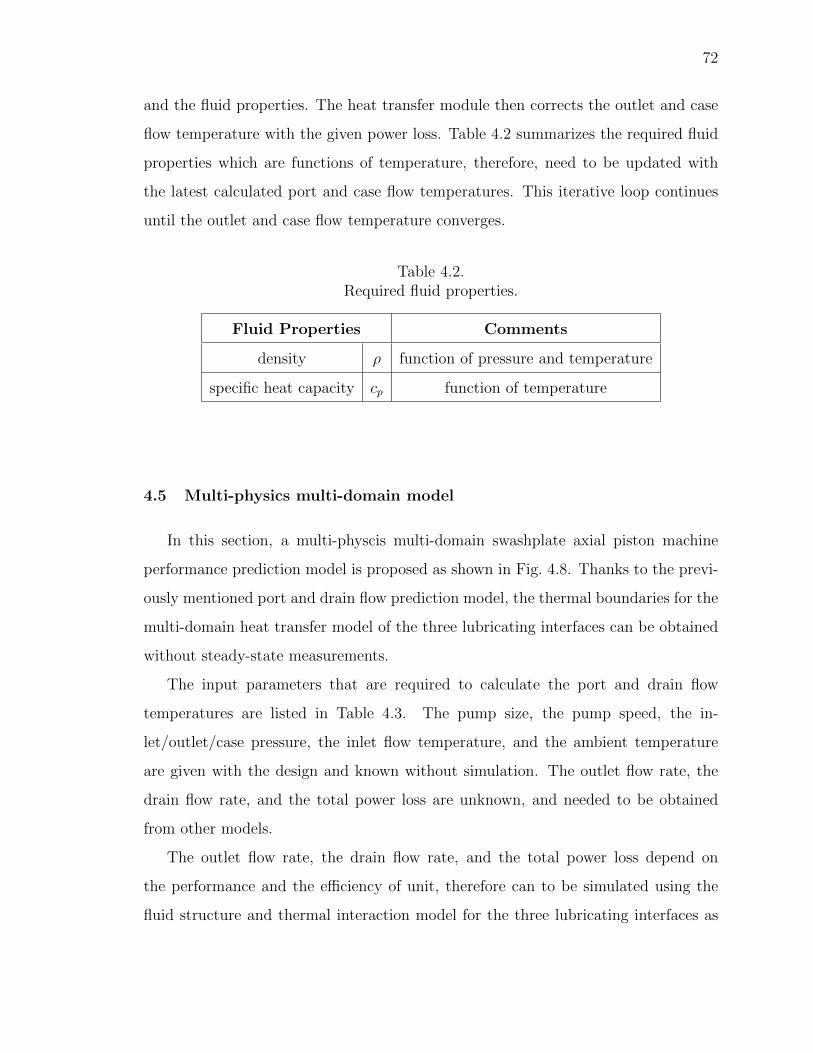
72

and the fluid properties. The heat transfer module then corrects the outlet and case

flow temperature with the given power loss. Table 4.2 summarizes the required fluid

properties which are functions of temperature, therefore, need to be updated with

the latest calculated port and case flow temperatures. This iterative loop continues

until the outlet and case flow temperature converges.

Table 4.2.Required fluid properties.

Fluid Properties Comments

density ρ function of pressure and temperature

specific heat capacity cp function of temperature

4.5 Multi-physics multi-domain model

In this section, a multi-physcis multi-domain swashplate axial piston machine

performance prediction model is proposed as shown in Fig. 4.8. Thanks to the previ-

ously mentioned port and drain flow prediction model, the thermal boundaries for the

multi-domain heat transfer model of the three lubricating interfaces can be obtained

without steady-state measurements.

The input parameters that are required to calculate the port and drain flow

temperatures are listed in Table 4.3. The pump size, the pump speed, the in-

let/outlet/case pressure, the inlet flow temperature, and the ambient temperature

are given with the design and known without simulation. The outlet flow rate, the

drain flow rate, and the total power loss are unknown, and needed to be obtained

from other models.

The outlet flow rate, the drain flow rate, and the total power loss depend on

the performance and the efficiency of unit, therefore can to be simulated using the

fluid structure and thermal interaction model for the three lubricating interfaces as

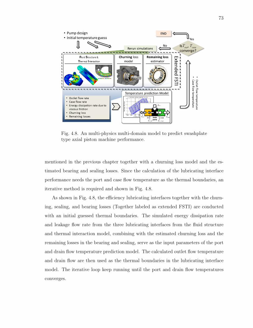
73

Fig. 4.8. An multi-physics multi-domain model to predict swashplatetype axial piston machine performance.

mentioned in the previous chapter together with a churning loss model and the es-

timated bearing and sealing losses. Since the calculation of the lubricating interface

performance needs the port and case flow temperature as the thermal boundaries, an

iterative method is required and shown in Fig. 4.8.

As shown in Fig. 4.8, the efficiency lubricating interfaces together with the churn-

ing, sealing, and bearing losses (Together labeled as extended FSTI) are conducted

with an initial guessed thermal boundaries. The simulated energy dissipation rate

and leakage flow rate from the three lubricating interfaces from the fluid structure

and thermal interaction model, combining with the estimated churning loss and the

remaining losses in the bearing and sealing, serve as the input parameters of the port

and drain flow temperature prediction model. The calculated outlet flow temperature

and drain flow are then used as the thermal boundaries in the lubricating interface

model. The iterative loop keep running until the port and drain flow temperatures

converges.

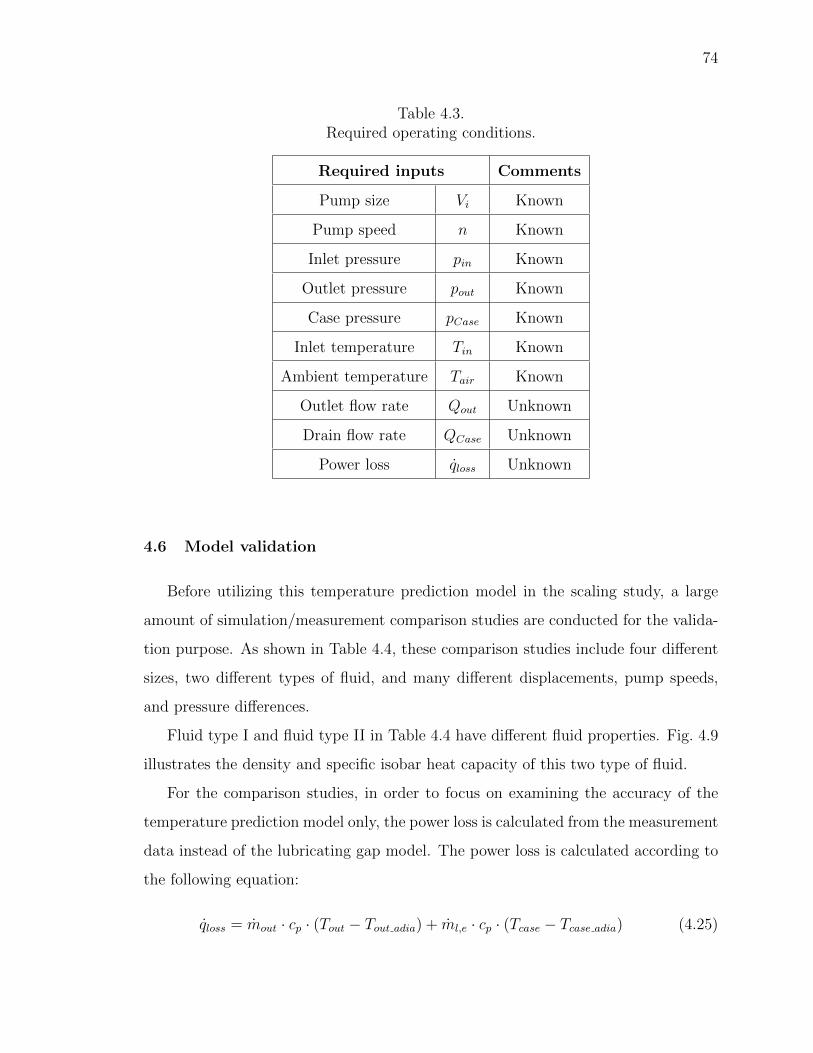
74

Table 4.3.Required operating conditions.

Required inputs Comments

Pump size Vi Known

Pump speed n Known

Inlet pressure pin Known

Outlet pressure pout Known

Case pressure pCase Known

Inlet temperature Tin Known

Ambient temperature Tair Known

Outlet flow rate Qout Unknown

Drain flow rate QCase Unknown

Power loss qloss Unknown

4.6 Model validation

Before utilizing this temperature prediction model in the scaling study, a large

amount of simulation/measurement comparison studies are conducted for the valida-

tion purpose. As shown in Table 4.4, these comparison studies include four different

sizes, two different types of fluid, and many different displacements, pump speeds,

and pressure differences.

Fluid type I and fluid type II in Table 4.4 have different fluid properties. Fig. 4.9

illustrates the density and specific isobar heat capacity of this two type of fluid.

For the comparison studies, in order to focus on examining the accuracy of the

temperature prediction model only, the power loss is calculated from the measurement

data instead of the lubricating gap model. The power loss is calculated according to

the following equation:

qloss = mout · cp · (Tout − Tout adia) + ml,e · cp · (Tcase − Tcase adia) (4.25)

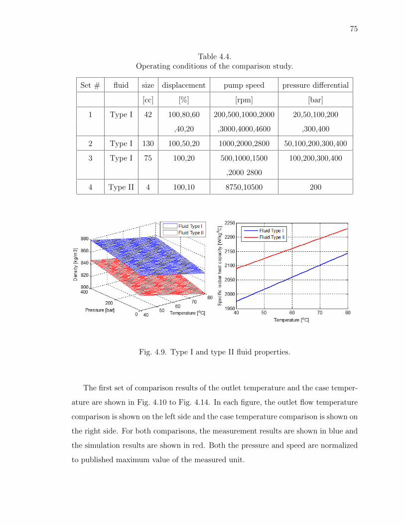
75

Table 4.4.Operating conditions of the comparison study.

Set # fluid size displacement pump speed pressure differential

[cc] [%] [rpm] [bar]

1 Type I 42 100,80,60 200,500,1000,2000 20,50,100,200

,40,20 ,3000,4000,4600 ,300,400

2 Type I 130 100,50,20 1000,2000,2800 50,100,200,300,400

3 Type I 75 100,20 500,1000,1500 100,200,300,400

,2000 2800

4 Type II 4 100,10 8750,10500 200

Fig. 4.9. Type I and type II fluid properties.

The first set of comparison results of the outlet temperature and the case temper-

ature are shown in Fig. 4.10 to Fig. 4.14. In each figure, the outlet flow temperature

comparison is shown on the left side and the case temperature comparison is shown on

the right side. For both comparisons, the measurement results are shown in blue and

the simulation results are shown in red. Both the pressure and speed are normalized

to published maximum value of the measured unit.

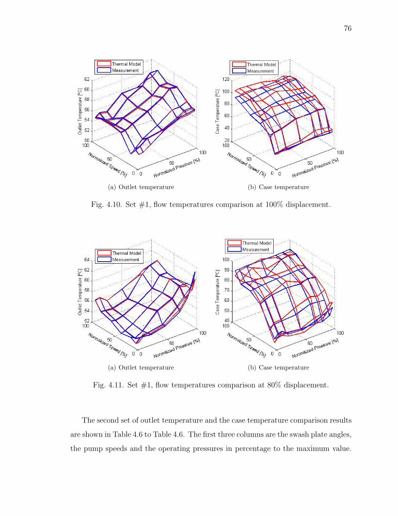
76

(a) Outlet temperature (b) Case temperature

Fig. 4.10. Set #1, flow temperatures comparison at 100% displacement.



The second set of outlet temperature and the case temperature comparison results

are shown in Table 4.6 to Table 4.6. The first three columns are the swash plate angles,

the pump speeds and the operating pressures in percentage to the maximum value.

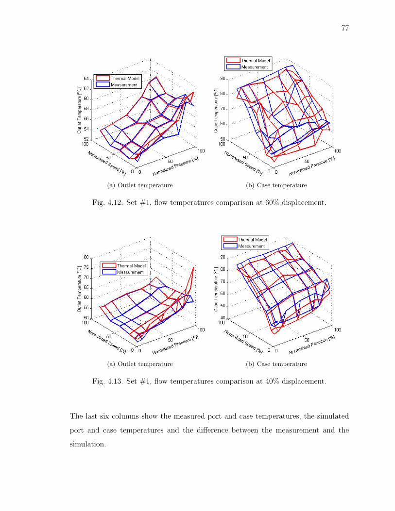
77





The last six columns show the measured port and case temperatures, the simulated

port and case temperatures and the difference between the measurement and the

simulation.

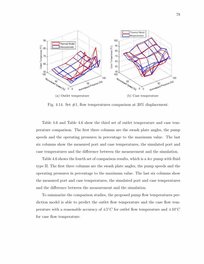
78



Table 4.6 and Table 4.6 show the third set of outlet temperature and case tem-

perature comparison. The first three columns are the swash plate angles, the pump

speeds and the operating pressures in percentage to the maximum value. The last

six columns show the measured port and case temperatures, the simulated port and

case temperatures and the difference between the measurement and the simulation.

Table 4.6 shows the fourth set of comparison results, which is a 4cc pump with fluid

type II. The first three columns are the swash plate angles, the pump speeds and the

operating pressures in percentage to the maximum value. The last six columns show

the measured port and case temperatures, the simulated port and case temperatures

and the difference between the measurement and the simulation.

To summarize the comparison studies, the proposed pump flow temperatures pre-

diction model is able to predict the outlet flow temperature and the case flow tem-

perature with a reasonable accuracy of ±5◦C for outlet flow temperature and ±10◦C

for case flow temperature.

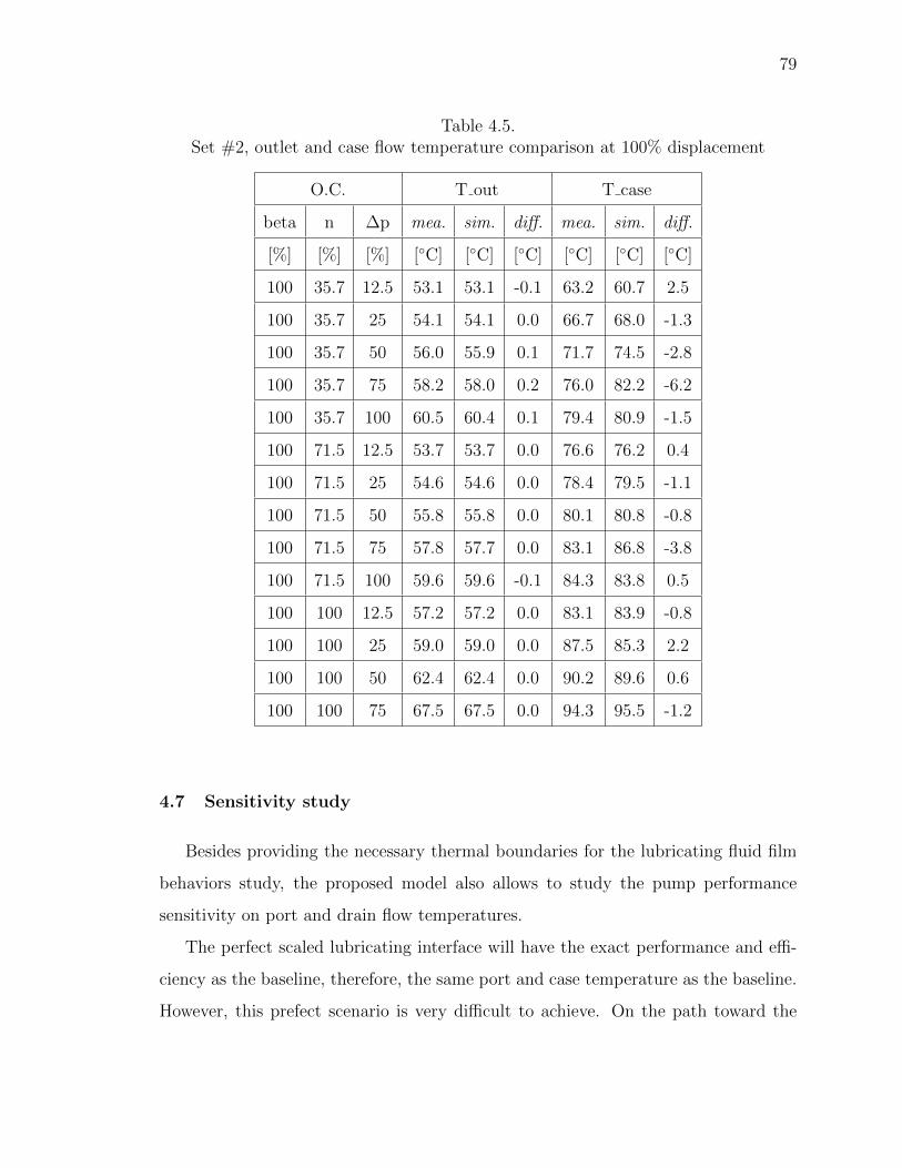
79

Table 4.5.Set #2, outlet and case flow temperature comparison at 100% displacement

O.C. T out T case

beta n ∆p mea. sim. diff. mea. sim. diff.

[%] [%] [%] [◦C] [◦C] [◦C] [◦C] [◦C] [◦C]

100 35.7 12.5 53.1 53.1 -0.1 63.2 60.7 2.5

100 35.7 25 54.1 54.1 0.0 66.7 68.0 -1.3

100 35.7 50 56.0 55.9 0.1 71.7 74.5 -2.8

100 35.7 75 58.2 58.0 0.2 76.0 82.2 -6.2

100 35.7 100 60.5 60.4 0.1 79.4 80.9 -1.5

100 71.5 12.5 53.7 53.7 0.0 76.6 76.2 0.4

100 71.5 25 54.6 54.6 0.0 78.4 79.5 -1.1

100 71.5 50 55.8 55.8 0.0 80.1 80.8 -0.8

100 71.5 75 57.8 57.7 0.0 83.1 86.8 -3.8

100 71.5 100 59.6 59.6 -0.1 84.3 83.8 0.5

100 100 12.5 57.2 57.2 0.0 83.1 83.9 -0.8

100 100 25 59.0 59.0 0.0 87.5 85.3 2.2

100 100 50 62.4 62.4 0.0 90.2 89.6 0.6

100 100 75 67.5 67.5 0.0 94.3 95.5 -1.2

4.7 Sensitivity study

Besides providing the necessary thermal boundaries for the lubricating fluid film

behaviors study, the proposed model also allows to study the pump performance

sensitivity on port and drain flow temperatures.

The perfect scaled lubricating interface will have the exact performance and effi-

ciency as the baseline, therefore, the same port and case temperature as the baseline.

However, this prefect scenario is very difficult to achieve. On the path toward the

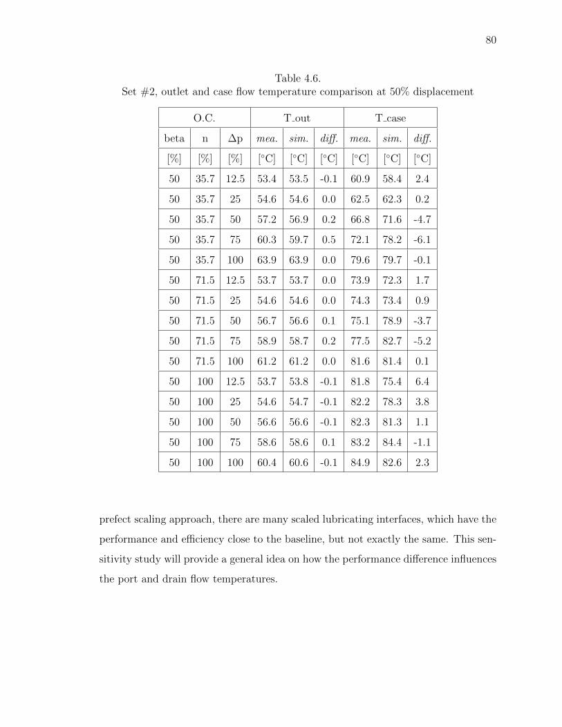
80


O.C. T out T case


[%] [%] [%] [◦C] [◦C] [◦C] [◦C] [◦C] [◦C]

50 35.7 12.5 53.4 53.5 -0.1 60.9 58.4 2.4

50 35.7 25 54.6 54.6 0.0 62.5 62.3 0.2

50 35.7 50 57.2 56.9 0.2 66.8 71.6 -4.7

50 35.7 75 60.3 59.7 0.5 72.1 78.2 -6.1

50 35.7 100 63.9 63.9 0.0 79.6 79.7 -0.1

50 71.5 12.5 53.7 53.7 0.0 73.9 72.3 1.7

50 71.5 25 54.6 54.6 0.0 74.3 73.4 0.9

50 71.5 50 56.7 56.6 0.1 75.1 78.9 -3.7

50 71.5 75 58.9 58.7 0.2 77.5 82.7 -5.2

50 71.5 100 61.2 61.2 0.0 81.6 81.4 0.1

50 100 12.5 53.7 53.8 -0.1 81.8 75.4 6.4

50 100 25 54.6 54.7 -0.1 82.2 78.3 3.8

50 100 50 56.6 56.6 -0.1 82.3 81.3 1.1

50 100 75 58.6 58.6 0.1 83.2 84.4 -1.1

50 100 100 60.4 60.6 -0.1 84.9 82.6 2.3

prefect scaling approach, there are many scaled lubricating interfaces, which have the

performance and efficiency close to the baseline, but not exactly the same. This sen-

sitivity study will provide a general idea on how the performance difference influences

the port and drain flow temperatures.

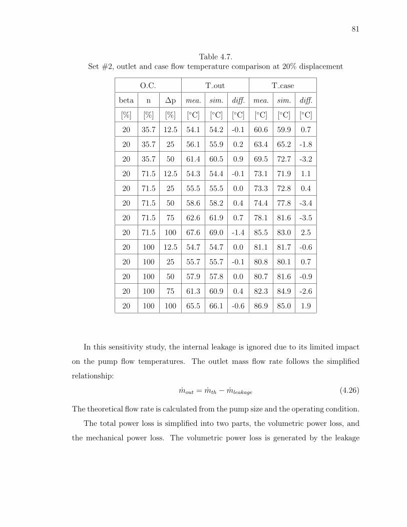
81


O.C. T out T case


[%] [%] [%] [◦C] [◦C] [◦C] [◦C] [◦C] [◦C]

20 35.7 12.5 54.1 54.2 -0.1 60.6 59.9 0.7

20 35.7 25 56.1 55.9 0.2 63.4 65.2 -1.8

20 35.7 50 61.4 60.5 0.9 69.5 72.7 -3.2

20 71.5 12.5 54.3 54.4 -0.1 73.1 71.9 1.1

20 71.5 25 55.5 55.5 0.0 73.3 72.8 0.4

20 71.5 50 58.6 58.2 0.4 74.4 77.8 -3.4

20 71.5 75 62.6 61.9 0.7 78.1 81.6 -3.5

20 71.5 100 67.6 69.0 -1.4 85.5 83.0 2.5

20 100 12.5 54.7 54.7 0.0 81.1 81.7 -0.6

20 100 25 55.7 55.7 -0.1 80.8 80.1 0.7

20 100 50 57.9 57.8 0.0 80.7 81.6 -0.9

20 100 75 61.3 60.9 0.4 82.3 84.9 -2.6

20 100 100 65.5 66.1 -0.6 86.9 85.0 1.9

In this sensitivity study, the internal leakage is ignored due to its limited impact

on the pump flow temperatures. The outlet mass flow rate follows the simplified

relationship:

mout = mth − mleakage (4.26)

The theoretical flow rate is calculated from the pump size and the operating condition.

The total power loss is simplified into two parts, the volumetric power loss, and

the mechanical power loss. The volumetric power loss is generated by the leakage

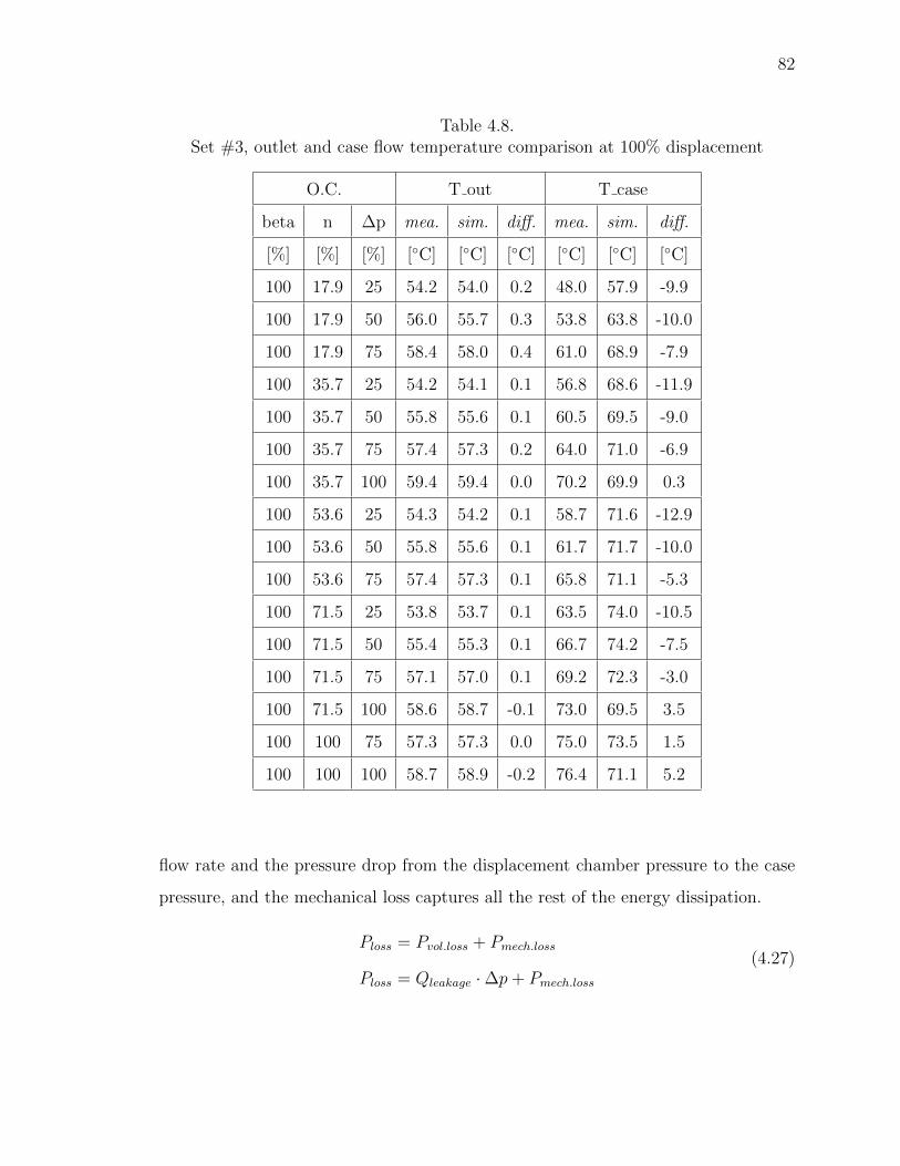
82


O.C. T out T case


[%] [%] [%] [◦C] [◦C] [◦C] [◦C] [◦C] [◦C]

100 17.9 25 54.2 54.0 0.2 48.0 57.9 -9.9

100 17.9 50 56.0 55.7 0.3 53.8 63.8 -10.0

100 17.9 75 58.4 58.0 0.4 61.0 68.9 -7.9

100 35.7 25 54.2 54.1 0.1 56.8 68.6 -11.9

100 35.7 50 55.8 55.6 0.1 60.5 69.5 -9.0

100 35.7 75 57.4 57.3 0.2 64.0 71.0 -6.9

100 35.7 100 59.4 59.4 0.0 70.2 69.9 0.3

100 53.6 25 54.3 54.2 0.1 58.7 71.6 -12.9

100 53.6 50 55.8 55.6 0.1 61.7 71.7 -10.0

100 53.6 75 57.4 57.3 0.1 65.8 71.1 -5.3

100 71.5 25 53.8 53.7 0.1 63.5 74.0 -10.5

100 71.5 50 55.4 55.3 0.1 66.7 74.2 -7.5

100 71.5 75 57.1 57.0 0.1 69.2 72.3 -3.0

100 71.5 100 58.6 58.7 -0.1 73.0 69.5 3.5

100 100 75 57.3 57.3 0.0 75.0 73.5 1.5

100 100 100 58.7 58.9 -0.2 76.4 71.1 5.2

flow rate and the pressure drop from the displacement chamber pressure to the case

pressure, and the mechanical loss captures all the rest of the energy dissipation.

Ploss = Pvol.loss + Pmech.loss

Ploss = Qleakage ·∆p+ Pmech.loss

(4.27)

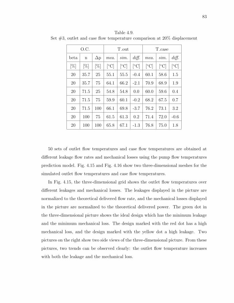
83


O.C. T out T case


[%] [%] [%] [◦C] [◦C] [◦C] [◦C] [◦C] [◦C]

20 35.7 25 55.1 55.5 -0.4 60.1 58.6 1.5

20 35.7 75 64.1 66.2 -2.1 70.9 68.9 1.9

20 71.5 25 54.8 54.8 0.0 60.0 59.6 0.4

20 71.5 75 59.9 60.1 -0.2 68.2 67.5 0.7

20 71.5 100 66.1 69.8 -3.7 76.2 73.1 3.2

20 100 75 61.5 61.3 0.2 71.4 72.0 -0.6

20 100 100 65.8 67.1 -1.3 76.8 75.0 1.8

50 sets of outlet flow temperatures and case flow temperatures are obtained at

different leakage flow rates and mechanical losses using the pump flow temperatures

prediction model. Fig. 4.15 and Fig. 4.16 show two three-dimensional meshes for the

simulated outlet flow temperatures and case flow temperatures.

In Fig. 4.15, the three-dimensional grid shows the outlet flow temperatures over

different leakages and mechanical losses. The leakages displayed in the picture are

normalized to the theoretical delivered flow rate, and the mechanical losses displayed

in the picture are normalized to the theoretical delivered power. The green dot in

the three-dimensional picture shows the ideal design which has the minimum leakage

and the minimum mechanical loss. The design marked with the red dot has a high

mechanical loss, and the design marked with the yellow dot a high leakage. Two

pictures on the right show two side views of the three-dimensional picture. From these

pictures, two trends can be observed clearly: the outlet flow temperature increases

with both the leakage and the mechanical loss.

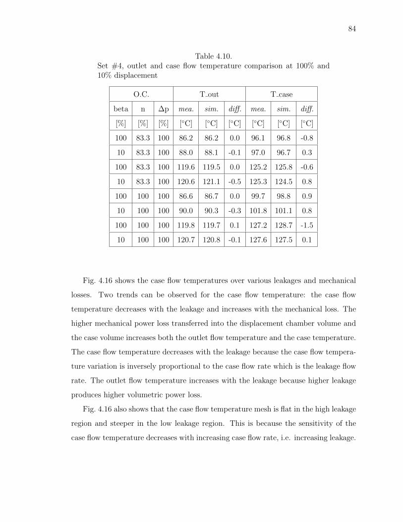
84

Table 4.10.Set #4, outlet and case flow temperature comparison at 100% and10% displacement

O.C. T out T case


[%] [%] [%] [◦C] [◦C] [◦C] [◦C] [◦C] [◦C]

100 83.3 100 86.2 86.2 0.0 96.1 96.8 -0.8

10 83.3 100 88.0 88.1 -0.1 97.0 96.7 0.3

100 83.3 100 119.6 119.5 0.0 125.2 125.8 -0.6

10 83.3 100 120.6 121.1 -0.5 125.3 124.5 0.8

100 100 100 86.6 86.7 0.0 99.7 98.8 0.9

10 100 100 90.0 90.3 -0.3 101.8 101.1 0.8

100 100 100 119.8 119.7 0.1 127.2 128.7 -1.5

10 100 100 120.7 120.8 -0.1 127.6 127.5 0.1

Fig. 4.16 shows the case flow temperatures over various leakages and mechanical

losses. Two trends can be observed for the case flow temperature: the case flow

temperature decreases with the leakage and increases with the mechanical loss. The

higher mechanical power loss transferred into the displacement chamber volume and

the case volume increases both the outlet flow temperature and the case temperature.

The case flow temperature decreases with the leakage because the case flow tempera-

ture variation is inversely proportional to the case flow rate which is the leakage flow

rate. The outlet flow temperature increases with the leakage because higher leakage

produces higher volumetric power loss.

Fig. 4.16 also shows that the case flow temperature mesh is flat in the high leakage

region and steeper in the low leakage region. This is because the sensitivity of the

case flow temperature decreases with increasing case flow rate, i.e. increasing leakage.

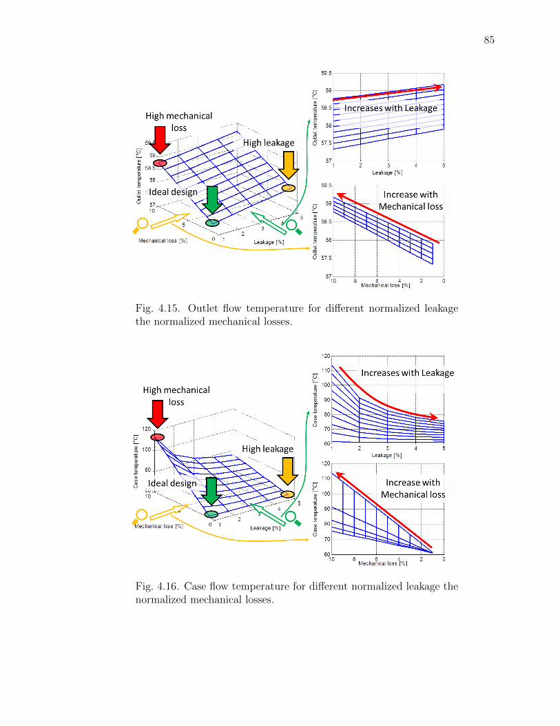
85

Fig. 4.15. Outlet flow temperature for different normalized leakagethe normalized mechanical losses.

Fig. 4.16. Case flow temperature for different normalized leakage thenormalized mechanical losses.

86

To conclude this sensitivity study, the machine performance will have a small

impact on the port and case flow temperature when the normalized leakage is high.

However, when normalized leakage is low, the case temperature increases dramatically

with the mechanical loss. The high leakage flow temperature will then cause low fluid

viscosity, therefore unfavorable load support in the lubricating gap, and more thermal

deformation, which can be dangerous in some designs.

4.8 Conclusion

In this chapter, a novel outlet and case flow temperatures prediction model for

axial piston machine is proposed. The model calculates the port temperatures con-

sidering the compression-expansion effect and the heat generation and heat transfer

in and between the solid and the fluid domain. The model is designed to apply on

pumps and motors at any size by scaling the coefficients with the respective linear

scaling factor. Over three hundred measured outlet and case flow temperatures have

been used to compare to the simulated results. The operating conditions include four

different unit size from 4 cc to 130 cc, two different types of fluid, from 10% to 100%

displacement, from 200 rpm to 10500 rpm, from 20 bar to 400 bar. The comparison

results prove that the proposed model is capable to predict the outlet and case flow

temperatures for unit with any size at any operating condition.

This proposed port temperatures prediction model allows the previously men-

tioned fluid structure and thermal interaction model to be used for virtual prototyping

and virtual optimization without any measurement data.

A sensitivity study is conducted using the proposed temperature prediction model.

The sensitivity study results can be used to reduce the required computational time

for the iterative pump and motor performance calculation. More sensitivity studies

were conducted within this research, and are detailed in [44].

87

5. THE SCALING OF PHYSICAL PHENOMENA IN

AXIAL PISTON MACHINES

The energy efficiency of axial piston machines do not remind the same after scaling

due to the size-dependent physics of the three tribological lubricating interfaces. In

this chapter, the size-dependence of physics that determines the behavior of the three

lubricating interfaces, including the hydrostatic/hydrodynamic pressure distribution

in fluid domain, the elastic deformation due to pressure and thermal load in solid

domain, and the heat transfer in the fluid and solid domains, are investigated using

scalable dimensions. The findings are used to provide a guide to scale the lubricating

interface while compensating the non-scalable physical phenomena.

The scalable or non-scalable physical phenomenon is defined as either it follows the

linear scaling law, such as pressure, temperature, and translational velocity remind

the same, distance and displacement follows the first order of the linear scaling factor,

area, power, and flow rate follow the second order of the linear scaling factor, and

mass and volume follow the third order of the linear scaling factor.

5.1 Linear scaling method (conventional approach)

Before explaining size-dependent physics, an example is given to demonstrate the

performance difference of the three interfaces before and after scaling according to

the linear scaling law. The scaling law is defined as scaling the axial piston machine

proportionally, such that the ratio of one design parameter to another is maintained.

The operating speed is scaled to keep the relative sliding speed between the parts that

form the tribological interfaces constant. For this example, a Sauer-Danfoss S90 75cc

unit is selected as the baseline unit. This baseline is linearly scaled to two different

sizes. The smaller one is scaled based on the linear factorλ of 0.5, and the bigger one

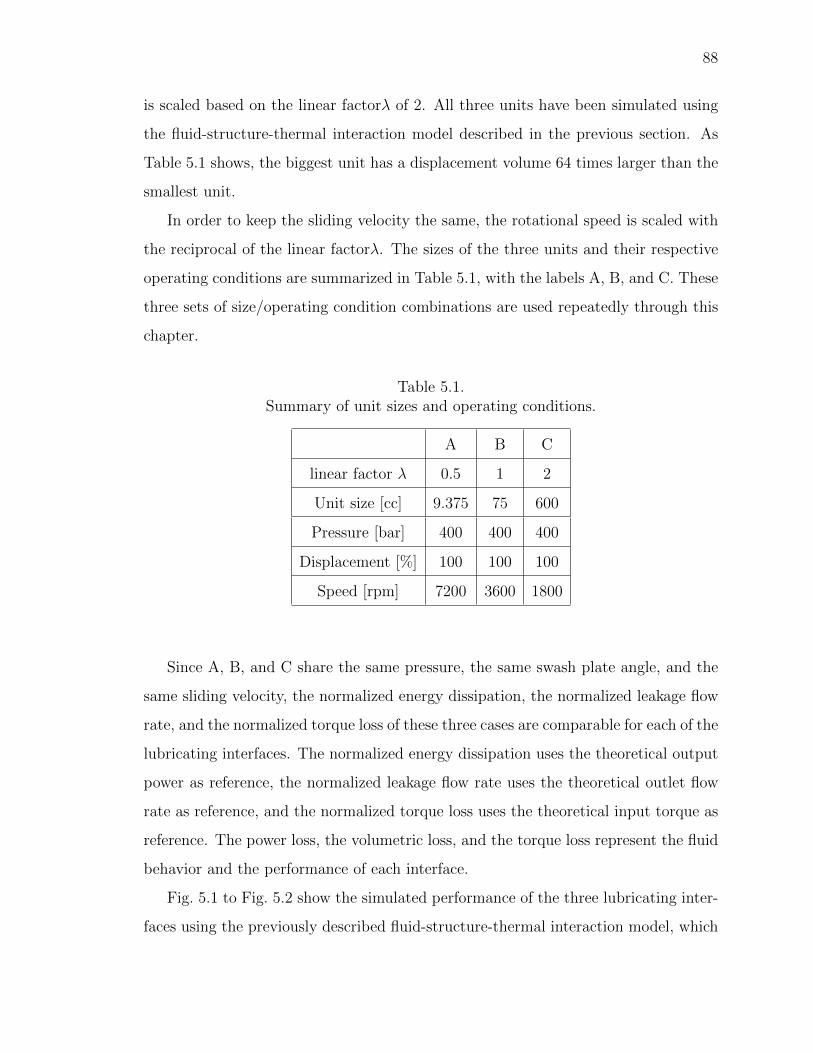
88

is scaled based on the linear factorλ of 2. All three units have been simulated using

the fluid-structure-thermal interaction model described in the previous section. As

Table 5.1 shows, the biggest unit has a displacement volume 64 times larger than the

smallest unit.

In order to keep the sliding velocity the same, the rotational speed is scaled with

the reciprocal of the linear factorλ. The sizes of the three units and their respective

operating conditions are summarized in Table 5.1, with the labels A, B, and C. These

three sets of size/operating condition combinations are used repeatedly through this

chapter.

Table 5.1.Summary of unit sizes and operating conditions.

A B C

linear factor λ 0.5 1 2

Unit size [cc] 9.375 75 600

Pressure [bar] 400 400 400

Displacement [%] 100 100 100

Speed [rpm] 7200 3600 1800

Since A, B, and C share the same pressure, the same swash plate angle, and the

same sliding velocity, the normalized energy dissipation, the normalized leakage flow

rate, and the normalized torque loss of these three cases are comparable for each of the

lubricating interfaces. The normalized energy dissipation uses the theoretical output

power as reference, the normalized leakage flow rate uses the theoretical outlet flow

rate as reference, and the normalized torque loss uses the theoretical input torque as

reference. The power loss, the volumetric loss, and the torque loss represent the fluid

behavior and the performance of each interface.

Fig. 5.1 to Fig. 5.2 show the simulated performance of the three lubricating inter-

faces using the previously described fluid-structure-thermal interaction model, which

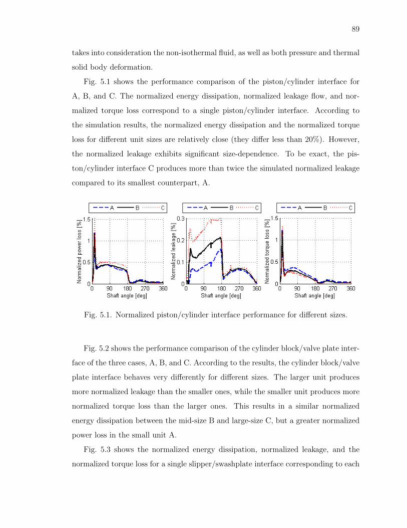
89

takes into consideration the non-isothermal fluid, as well as both pressure and thermal

solid body deformation.

Fig. 5.1 shows the performance comparison of the piston/cylinder interface for

A, B, and C. The normalized energy dissipation, normalized leakage flow, and nor-

malized torque loss correspond to a single piston/cylinder interface. According to

the simulation results, the normalized energy dissipation and the normalized torque

loss for different unit sizes are relatively close (they differ less than 20%). However,

the normalized leakage exhibits significant size-dependence. To be exact, the pis-

ton/cylinder interface C produces more than twice the simulated normalized leakage

compared to its smallest counterpart, A.

Fig. 5.1. Normalized piston/cylinder interface performance for different sizes.

Fig. 5.2 shows the performance comparison of the cylinder block/valve plate inter-

face of the three cases, A, B, and C. According to the results, the cylinder block/valve

plate interface behaves very differently for different sizes. The larger unit produces

more normalized leakage than the smaller ones, while the smaller unit produces more

normalized torque loss than the larger ones. This results in a similar normalized

energy dissipation between the mid-size B and large-size C, but a greater normalized

power loss in the small unit A.

Fig. 5.3 shows the normalized energy dissipation, normalized leakage, and the

normalized torque loss for a single slipper/swashplate interface corresponding to each

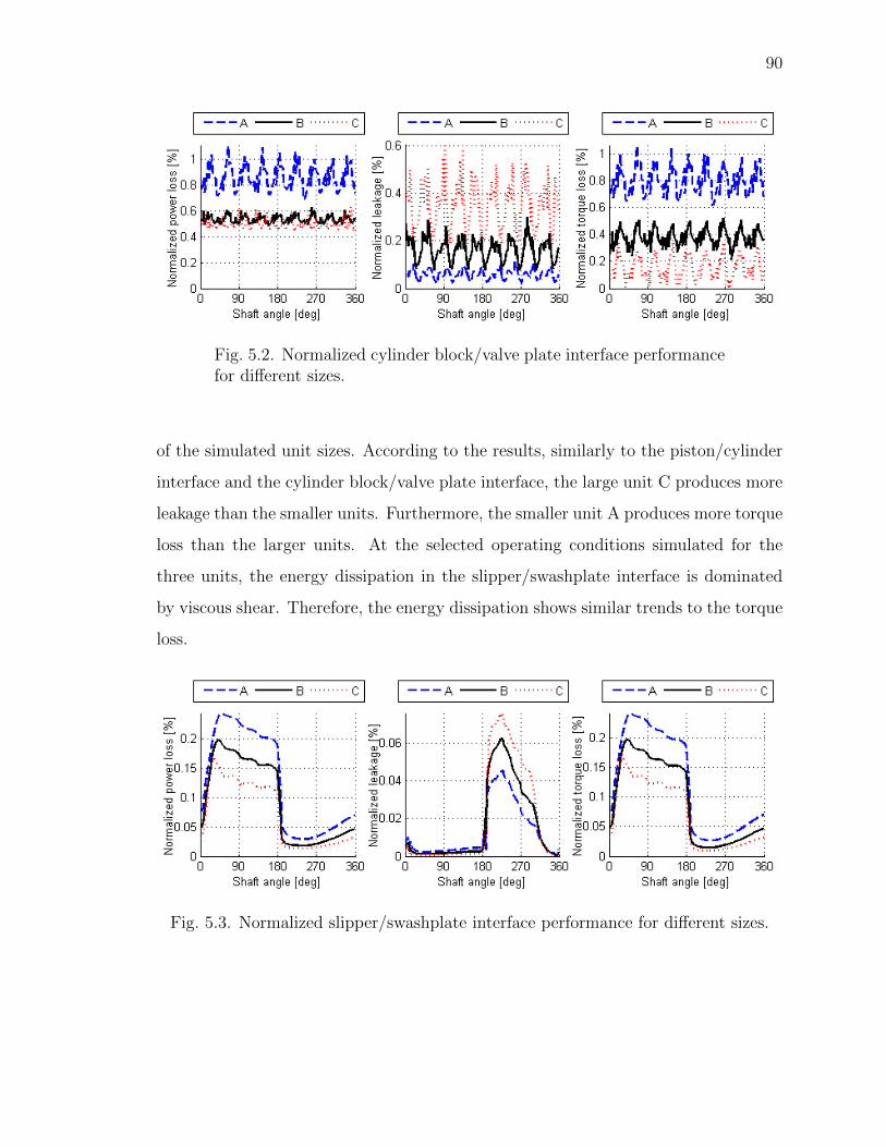
90

Fig. 5.2. Normalized cylinder block/valve plate interface performancefor different sizes.

of the simulated unit sizes. According to the results, similarly to the piston/cylinder

interface and the cylinder block/valve plate interface, the large unit C produces more

leakage than the smaller units. Furthermore, the smaller unit A produces more torque

loss than the larger units. At the selected operating conditions simulated for the

three units, the energy dissipation in the slipper/swashplate interface is dominated

by viscous shear. Therefore, the energy dissipation shows similar trends to the torque

loss.

Fig. 5.3. Normalized slipper/swashplate interface performance for different sizes.

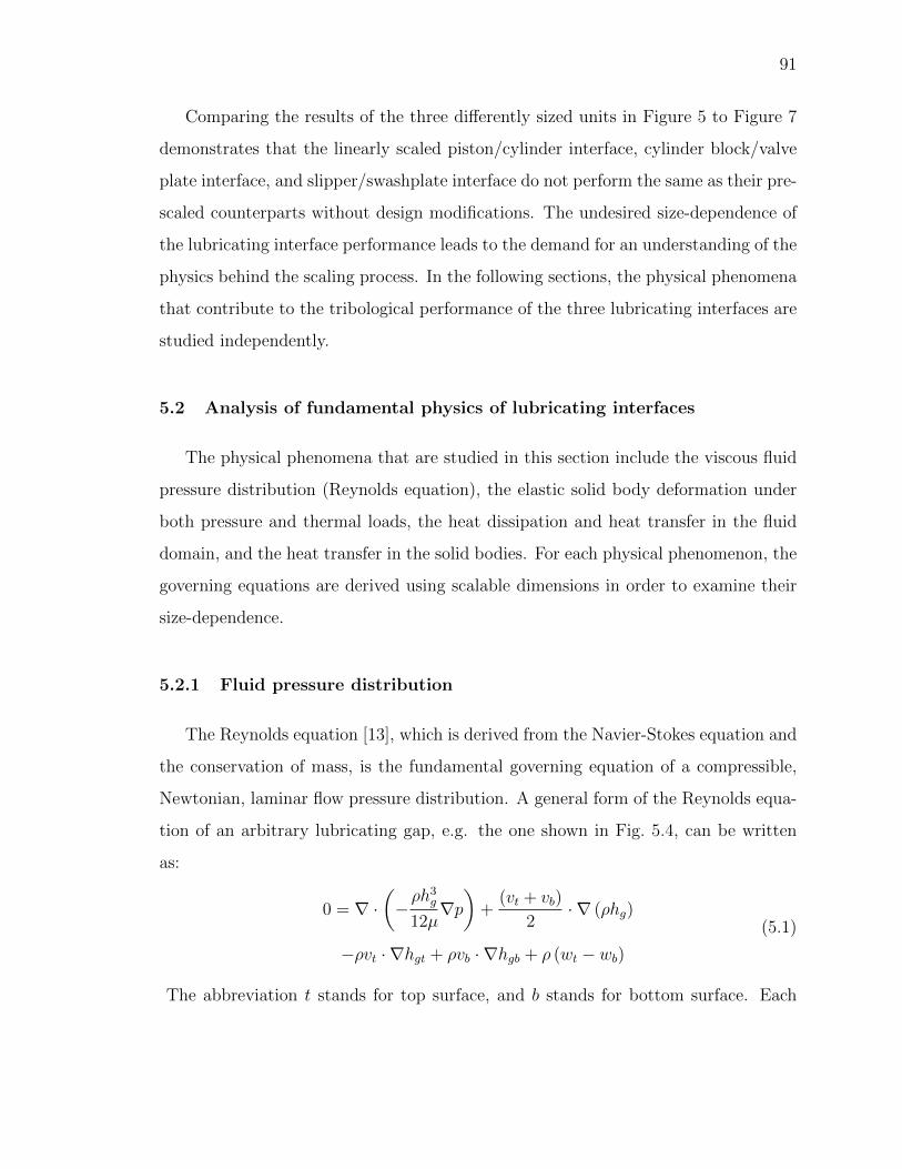
91

Comparing the results of the three differently sized units in Figure 5 to Figure 7

demonstrates that the linearly scaled piston/cylinder interface, cylinder block/valve

plate interface, and slipper/swashplate interface do not perform the same as their pre-

scaled counterparts without design modifications. The undesired size-dependence of

the lubricating interface performance leads to the demand for an understanding of the

physics behind the scaling process. In the following sections, the physical phenomena

that contribute to the tribological performance of the three lubricating interfaces are

studied independently.

5.2 Analysis of fundamental physics of lubricating interfaces

The physical phenomena that are studied in this section include the viscous fluid

pressure distribution (Reynolds equation), the elastic solid body deformation under

both pressure and thermal loads, the heat dissipation and heat transfer in the fluid

domain, and the heat transfer in the solid bodies. For each physical phenomenon, the

governing equations are derived using scalable dimensions in order to examine their

size-dependence.

5.2.1 Fluid pressure distribution

The Reynolds equation [13], which is derived from the Navier-Stokes equation and

the conservation of mass, is the fundamental governing equation of a compressible,

Newtonian, laminar flow pressure distribution. A general form of the Reynolds equa-

tion of an arbitrary lubricating gap, e.g. the one shown in Fig. 5.4, can be written

as:

0 = ∇ ·(−ρh3g12µ∇p)

+(vt + vb)

2· ∇ (ρhg)

−ρvt · ∇hgt + ρvb · ∇hgb + ρ (wt − wb)(5.1)

The abbreviation t stands for top surface, and b stands for bottom surface. Each

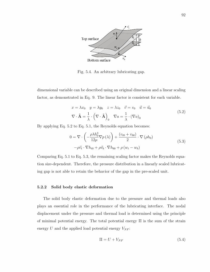
92

Fig. 5.4. An arbitrary lubricating gap.

dimensional variable can be described using an original dimension and a linear scaling

factor, as demonstrated in Eq. 9. The linear factor is consistent for each variable.

x = λx0 y = λy0 z = λz0 ~v = v0 ~u = ~u0

∇ · A =1

λ·(∇ · A

)0∇a =

1

λ· (∇a)0

(5.2)

By applying Eq. 5.2 to Eq. 5.1, the Reynolds equation becomes:

0 = ∇ ·(−ρλh

30

12µ∇p (λ)

)+

(vt0 + vb0)

2· ∇ (ρh0)

−ρ~vt · ∇ht0 + ρ~vb · ∇hb0 + ρ (wt − wb)(5.3)

Comparing Eq. 5.1 to Eq. 5.3, the remaining scaling factor makes the Reynolds equa-

tion size-dependent. Therefore, the pressure distribution in a linearly scaled lubricat-

ing gap is not able to retain the behavior of the gap in the pre-scaled unit.

5.2.2 Solid body elastic deformation

The solid body elastic deformation due to the pressure and thermal loads also

plays an essential role in the performance of the lubricating interface. The nodal

displacement under the pressure and thermal load is determined using the principle

of minimal potential energy. The total potential energy Π is the sum of the strain

energy U and the applied load potential energy VNF :

Π = U + VNF (5.4)

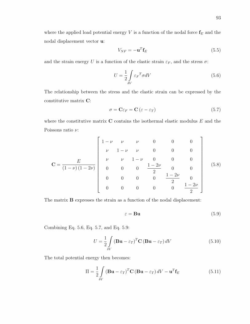
93

where the applied load potential energy V is a function of the nodal force fE and the

nodal displacement vector u:

VNF = −uT fE (5.5)

and the strain energy U is a function of the elastic strain εF , and the stress σ:

U =1

2

∫δV

εFTσdV (5.6)

The relationship between the stress and the elastic strain can be expressed by the

constitutive matrix C:

σ = CεF = C (ε− εT ) (5.7)

where the constitutive matrix C contains the isothermal elastic modulus E and the

Poissons ratio ν:

C =E

(1− ν) (1− 2ν)

1− ν ν ν 0 0 0

ν 1− ν ν 0 0 0

ν ν 1− ν 0 0 0

0 0 01− 2ν

20 0

0 0 0 01− 2ν

20

0 0 0 0 01− 2ν

2

(5.8)

The matrix B expresses the strain as a function of the nodal displacement:

ε = Bu (5.9)

Combining Eq. 5.6, Eq. 5.7, and Eq. 5.9:

U =1

2

∫δV

(Bu− εT )TC (Bu− εT ) dV (5.10)

The total potential energy then becomes:

Π =1

2

∫δV

(Bu− εT )TC (Bu− εT ) dV − uT fE (5.11)

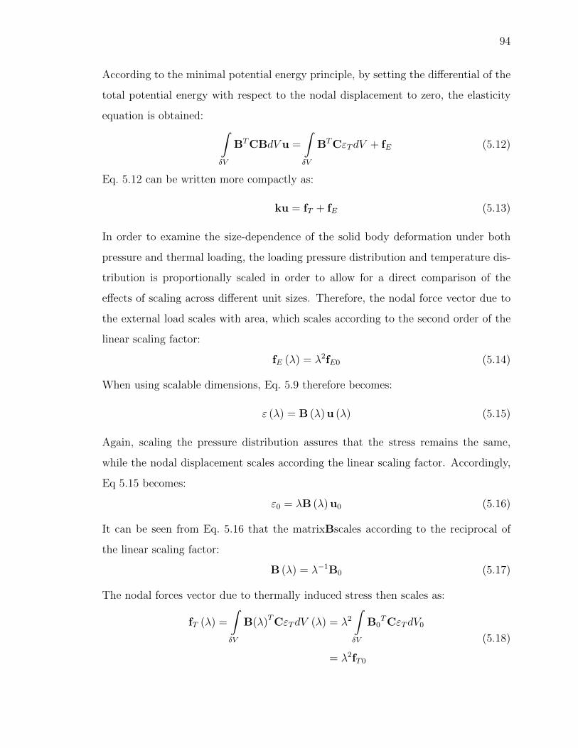
94

According to the minimal potential energy principle, by setting the differential of the

total potential energy with respect to the nodal displacement to zero, the elasticity

equation is obtained: ∫δV

BTCBdV u =

∫δV

BTCεTdV + fE (5.12)

Eq. 5.12 can be written more compactly as:

ku = fT + fE (5.13)

In order to examine the size-dependence of the solid body deformation under both

pressure and thermal loading, the loading pressure distribution and temperature dis-

tribution is proportionally scaled in order to allow for a direct comparison of the

effects of scaling across different unit sizes. Therefore, the nodal force vector due to

the external load scales with area, which scales according to the second order of the

linear scaling factor:

fE (λ) = λ2fE0 (5.14)

When using scalable dimensions, Eq. 5.9 therefore becomes:

ε (λ) = B (λ) u (λ) (5.15)

Again, scaling the pressure distribution assures that the stress remains the same,

while the nodal displacement scales according the linear scaling factor. Accordingly,

Eq 5.15 becomes:

ε0 = λB (λ) u0 (5.16)

It can be seen from Eq. 5.16 that the matrixBscales according to the reciprocal of

the linear scaling factor:

B (λ) = λ−1B0 (5.17)

The nodal forces vector due to thermally induced stress then scales as:

fT (λ) =

∫δV

B(λ)TCεTdV (λ) = λ2∫δV

B0TCεTdV0

= λ2fT0

(5.18)

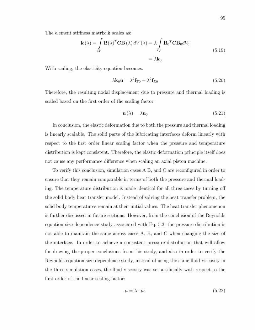
95

The element stiffness matrix k scales as:

k (λ) =

∫δV

B(λ)TCB (λ) dV (λ) = λ

∫δV

B0TCB0dV0

= λk0

(5.19)

With scaling, the elasticity equation becomes:

λk0u = λ2fT0 + λ2fE0 (5.20)

Therefore, the resulting nodal displacement due to pressure and thermal loading is

scaled based on the first order of the scaling factor:

u (λ) = λu0 (5.21)

In conclusion, the elastic deformation due to both the pressure and thermal loading

is linearly scalable. The solid parts of the lubricating interfaces deform linearly with

respect to the first order linear scaling factor when the pressure and temperature

distribution is kept consistent. Therefore, the elastic deformation principle itself does

not cause any performance difference when scaling an axial piston machine.

To verify this conclusion, simulation cases A B, and C are reconfigured in order to

ensure that they remain comparable in terms of both the pressure and thermal load-

ing. The temperature distribution is made identical for all three cases by turning off

the solid body heat transfer model. Instead of solving the heat transfer problem, the

solid body temperatures remain at their initial values. The heat transfer phenomenon

is further discussed in future sections. However, from the conclusion of the Reynolds

equation size dependence study associated with Eq. 5.3, the pressure distribution is

not able to maintain the same across cases A, B, and C when changing the size of

the interface. In order to achieve a consistent pressure distribution that will allow

for drawing the proper conclusions from this study, and also in order to verify the

Reynolds equation size-dependence study, instead of using the same fluid viscosity in

the three simulation cases, the fluid viscosity was set artificially with respect to the

first order of the linear scaling factor:

µ = λ · µ0 (5.22)

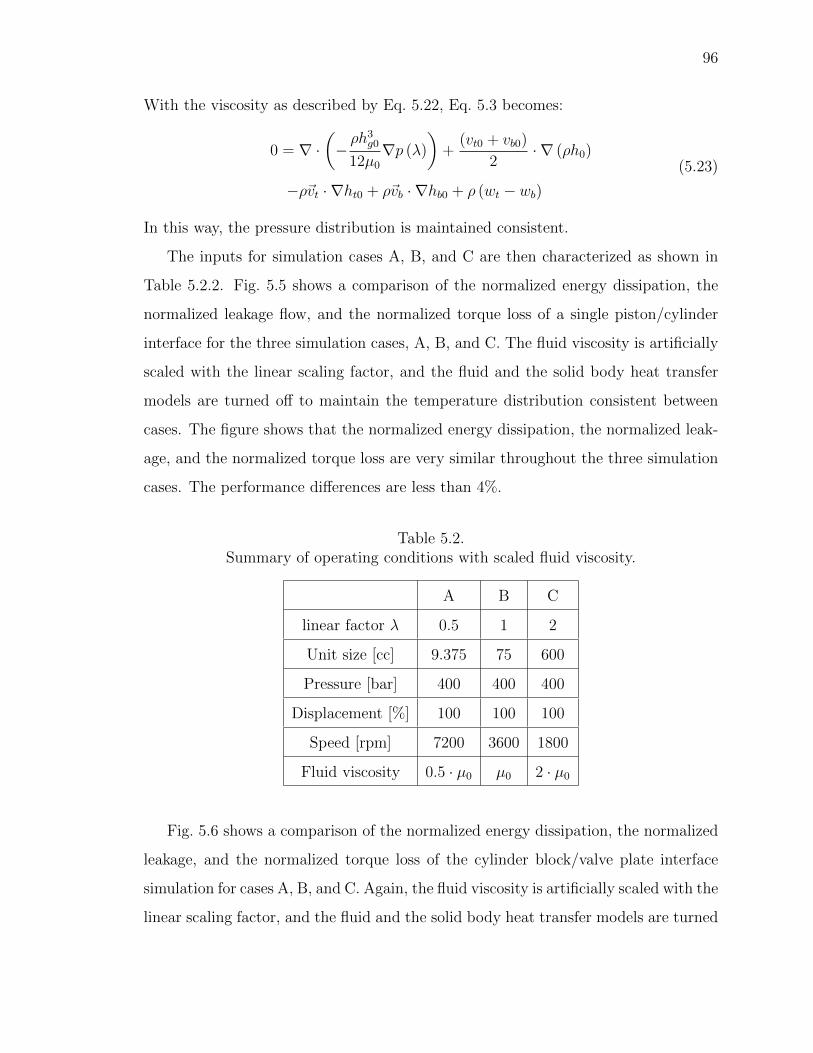
96

With the viscosity as described by Eq. 5.22, Eq. 5.3 becomes:

0 = ∇ ·(−ρh3g012µ0

∇p (λ)

)+

(vt0 + vb0)

2· ∇ (ρh0)

−ρ~vt · ∇ht0 + ρ~vb · ∇hb0 + ρ (wt − wb)(5.23)

In this way, the pressure distribution is maintained consistent.

The inputs for simulation cases A, B, and C are then characterized as shown in

Table 5.2.2. Fig. 5.5 shows a comparison of the normalized energy dissipation, the

normalized leakage flow, and the normalized torque loss of a single piston/cylinder

interface for the three simulation cases, A, B, and C. The fluid viscosity is artificially

scaled with the linear scaling factor, and the fluid and the solid body heat transfer

models are turned off to maintain the temperature distribution consistent between

cases. The figure shows that the normalized energy dissipation, the normalized leak-

age, and the normalized torque loss are very similar throughout the three simulation

cases. The performance differences are less than 4%.

Table 5.2.Summary of operating conditions with scaled fluid viscosity.

A B C


Unit size [cc] 9.375 75 600



Speed [rpm] 7200 3600 1800

Fluid viscosity 0.5 · µ0 µ0 2 · µ0

Fig. 5.6 shows a comparison of the normalized energy dissipation, the normalized

leakage, and the normalized torque loss of the cylinder block/valve plate interface

simulation for cases A, B, and C. Again, the fluid viscosity is artificially scaled with the

linear scaling factor, and the fluid and the solid body heat transfer models are turned

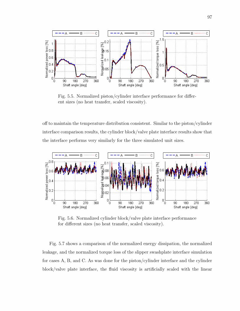
97

Fig. 5.5. Normalized piston/cylinder interface performance for differ-ent sizes (no heat transfer, scaled viscosity).

off to maintain the temperature distribution consistent. Similar to the piston/cylinder

interface comparison results, the cylinder block/valve plate interface results show that

the interface performs very similarly for the three simulated unit sizes.

Fig. 5.6. Normalized cylinder block/valve plate interface performancefor different sizes (no heat transfer, scaled viscosity).


leakage, and the normalized torque loss of the slipper swashplate interface simulation

for cases A, B, and C. As was done for the piston/cylinder interface and the cylinder

block/valve plate interface, the fluid viscosity is artificially scaled with the linear

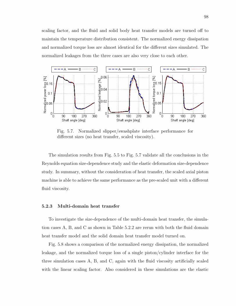
98

scaling factor, and the fluid and solid body heat transfer models are turned off to

maintain the temperature distribution consistent. The normalized energy dissipation

and normalized torque loss are almost identical for the different sizes simulated. The

normalized leakages from the three cases are also very close to each other.

Fig. 5.7. Normalized slipper/swashplate interface performance fordifferent sizes (no heat transfer, scaled viscosity).

The simulation results from Fig. 5.5 to Fig. 5.7 validate all the conclusions in the

Reynolds equation size-dependence study and the elastic deformation size-dependence

study. In summary, without the consideration of heat transfer, the scaled axial piston

machine is able to achieve the same performance as the pre-scaled unit with a different

fluid viscosity.

5.2.3 Multi-domain heat transfer

To investigate the size-dependence of the multi-domain heat transfer, the simula-

tion cases A, B, and C as shown in Table 5.2.2 are rerun with both the fluid domain

heat transfer model and the solid domain heat transfer model turned on.


leakage, and the normalized torque loss of a single piston/cylinder interface for the

three simulation cases A, B, and C, again with the fluid viscosity artificially scaled

with the linear scaling factor. Also considered in these simulations are the elastic

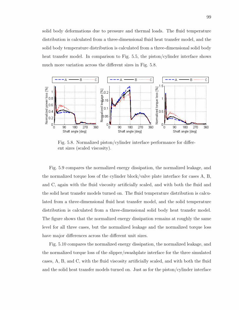
99

solid body deformations due to pressure and thermal loads. The fluid temperature

distribution is calculated from a three-dimensional fluid heat transfer model, and the

solid body temperature distribution is calculated from a three-dimensional solid body

heat transfer model. In comparison to Fig. 5.5, the piston/cylinder interface shows

much more variation across the different sizes in Fig. 5.8.

Fig. 5.8. Normalized piston/cylinder interface performance for differ-ent sizes (scaled viscosity).

Fig. 5.9 compares the normalized energy dissipation, the normalized leakage, and

the normalized torque loss of the cylinder block/valve plate interface for cases A, B,

and C, again with the fluid viscosity artificially scaled, and with both the fluid and

the solid heat transfer models turned on. The fluid temperature distribution is calcu-

lated from a three-dimensional fluid heat transfer model, and the solid temperature

distribution is calculated from a three-dimensional solid body heat transfer model.

The figure shows that the normalized energy dissipation remains at roughly the same

level for all three cases, but the normalized leakage and the normalized torque loss

have major differences across the different unit sizes.

Fig. 5.10 compares the normalized energy dissipation, the normalized leakage, and

the normalized torque loss of the slipper/swashplate interface for the three simulated

cases, A, B, and C, with the fluid viscosity artificially scaled, and with both the fluid

and the solid heat transfer models turned on. Just as for the piston/cylinder interface

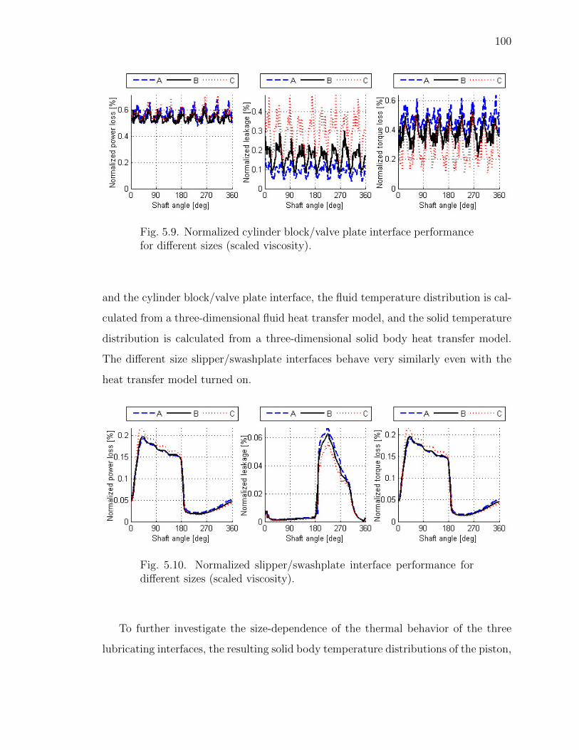
100

Fig. 5.9. Normalized cylinder block/valve plate interface performancefor different sizes (scaled viscosity).

and the cylinder block/valve plate interface, the fluid temperature distribution is cal-

culated from a three-dimensional fluid heat transfer model, and the solid temperature

distribution is calculated from a three-dimensional solid body heat transfer model.

The different size slipper/swashplate interfaces behave very similarly even with the

heat transfer model turned on.

Fig. 5.10. Normalized slipper/swashplate interface performance fordifferent sizes (scaled viscosity).

To further investigate the size-dependence of the thermal behavior of the three

lubricating interfaces, the resulting solid body temperature distributions of the piston,

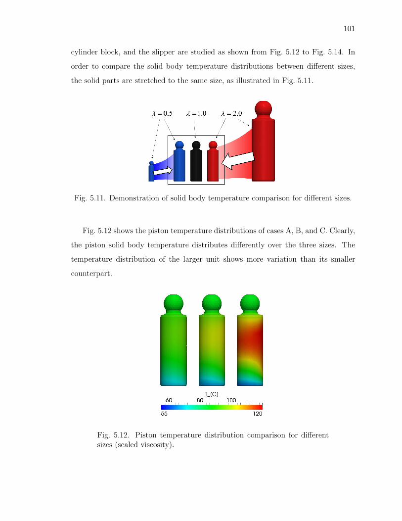
101

cylinder block, and the slipper are studied as shown from Fig. 5.12 to Fig. 5.14. In

order to compare the solid body temperature distributions between different sizes,

the solid parts are stretched to the same size, as illustrated in Fig. 5.11.

Fig. 5.11. Demonstration of solid body temperature comparison for different sizes.

Fig. 5.12 shows the piston temperature distributions of cases A, B, and C. Clearly,

the piston solid body temperature distributes differently over the three sizes. The

temperature distribution of the larger unit shows more variation than its smaller

counterpart.

Fig. 5.12. Piston temperature distribution comparison for differentsizes (scaled viscosity).

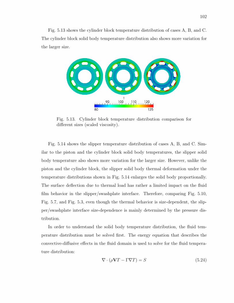
102

Fig. 5.13 shows the cylinder block temperature distribution of cases A, B, and C.

The cylinder block solid body temperature distribution also shows more variation for

the larger size.

Fig. 5.13. Cylinder block temperature distribution comparison fordifferent sizes (scaled viscosity).

Fig. 5.14 shows the slipper temperature distribution of cases A, B, and C. Sim-

ilar to the piston and the cylinder block solid body temperatures, the slipper solid

body temperature also shows more variation for the larger size. However, unlike the

piston and the cylinder block, the slipper solid body thermal deformation under the

temperature distributions shown in Fig. 5.14 enlarges the solid body proportionally.

The surface deflection due to thermal load has rather a limited impact on the fluid

film behavior in the slipper/swashplate interface. Therefore, comparing Fig. 5.10,

Fig. 5.7, and Fig. 5.3, even though the thermal behavior is size-dependent, the slip-

per/swashplate interface size-dependence is mainly determined by the pressure dis-

tribution.

In order to understand the solid body temperature distribution, the fluid tem-

perature distribution must be solved first. The energy equation that describes the

convective-diffusive effects in the fluid domain is used to solve for the fluid tempera-

ture distribution:

∇ · (ρVT − Γ∇T ) = S (5.24)

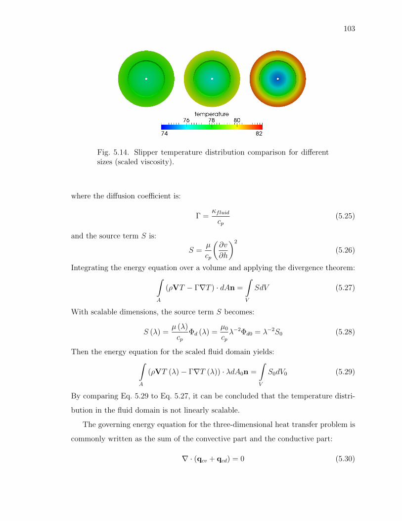
103

Fig. 5.14. Slipper temperature distribution comparison for differentsizes (scaled viscosity).

where the diffusion coefficient is:

Γ =κfluidcp

(5.25)

and the source term S is:

S =µ

cp

(∂v

∂h

)2

(5.26)

Integrating the energy equation over a volume and applying the divergence theorem:∫A

(ρVT − Γ∇T ) · dAn =

∫V

SdV (5.27)

With scalable dimensions, the source term S becomes:

S (λ) =µ (λ)

cpΦd (λ) =

µ0

cpλ−2Φd0 = λ−2S0 (5.28)

Then the energy equation for the scaled fluid domain yields:∫A

(ρVT (λ)− Γ∇T (λ)) · λdA0n =

∫V

S0dV0 (5.29)

By comparing Eq. 5.29 to Eq. 5.27, it can be concluded that the temperature distri-

bution in the fluid domain is not linearly scalable.

The governing energy equation for the three-dimensional heat transfer problem is

commonly written as the sum of the convective part and the conductive part:

∇ · (qcv + qcd) = 0 (5.30)

104

For a control volume, the energy equation yields:∫A

qcv · ndA+

∫V

∇ · qcddV = 0 (5.31)

There are two types of convection boundaries commonly applied to the solid body

surfaces:

Neumann boundary condition: The Neumann condition is applied to the run-

ning surfaces of the lubricating interface, where the heat flux into each of the

solid parts adjacent to the fluid can be calculated as the energy dissipation,

minus the energy taken away with the passing flow.

qcv · ndA =1

2

∫V

µΦddV −∫S

cpρVT · ndS

(5.32)

Mixed boundary condition: The mixed condition is applied on the surfaces where

the temperature of the surrounding environment is constant. The heat flux of

the mixed condition can be calculated using the solid body surface temperature,

the temperature of the surrounding environment, and a heat transfer coefficient.

qcv · ndA = h (TS − T∞) dA (5.33)

The conductive part of the energy equation yields:∫V

∇ · qcddV =

∫V

∇ · (−κsolid∇T ) dV (5.34)

When use scalable dimensions, the Neumann type convection boundary becomes:

qcv (λ) · ndA (λ) =1

2

∫V

µ (λ)λ−2Φd0λ3dV0 −

∫S

cpρVT · nλ2dS0

(5.35)

The mixed type convection boundary becomes:

qcv (λ) · ndA (λ) = h (TS − T∞)λ2dA0 = λ2qcv0 · ndA0 (5.36)

105

The conductive term of the energy equation scales as:∫V

∇ · (−κsolid∇T (λ)) dV (λ) = λ2∫V

∇ · (−κsolid∇T (λ)) dV0 (5.37)

Eq. 5.35, Eq. 5.36, and Eq. 5.37 show that the scaled solid body parts will result in

a different dimensional heat transfer performance than when using linear scaling.

So far, the analytical investigation of the temperature distribution in both the fluid

domain and the solid domain proved that the thermal characteristic of the lubricating

interface is not scalable. For the purposes of scientific research, the artificial size-

dependent viscosity in Eq. 5.22 was used in Eq. 5.28.

S (λ) = λ−1S0 (5.38)

Then the energy equation for the scaled fluid domain yields:∫A

(ρVT (λ)− Γ∇T (λ)) · dA0n =

∫V

S0dV0 (5.39)

To keep the temperature distribution consistent in the scaled fluid domain, the tem-

perature and the temperature gradient scale as:

T (λ) = T0

∇T (λ) = λ−1∇T0(5.40)

Eq. 5.39 then becomes:∫A

(ρVT0 − Γλ−1∇T0

)· dA0n =

∫V

S0dV0 (5.41)

Eq. 5.41 shows that consistency in the temperature distribution can be achieved if the

fluid is not only given the viscosity of Eq. 5.22, but also the following fluid diffusion

coefficient:

Γ (λ) = λΓ0 (5.42)

A similar approach can be used for the three-dimensional solid body heat transfer

analysis. Applying Eq. 5.22 to Eq. 5.35:

qcv (λ) · ndA (λ) =1

2

∫V

λµ0λ−2Φd0λ

3dV0 −∫S

cpρVT · nλ2dS0

= λ2qcv0 · ndA0

(5.43)

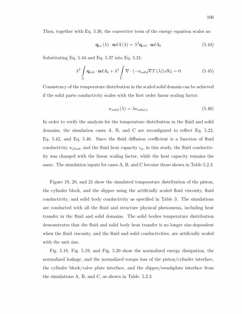
106

Then, together with Eq. 5.36, the convective term of the energy equation scales as:

qcv (λ) · ndA (λ) = λ2qcv0 · ndA0 (5.44)

Substituting Eq. 5.44 and Eq. 5.37 into Eq. 5.31:

λ2∫A

qcv0 · ndA0 + λ2∫V

∇ · (−κsolid∇T (λ)) dV0 = 0 (5.45)

Consistency of the temperature distribution in the scaled solid domain can be achieved

if the solid parts conductivity scales with the first order linear scaling factor:

κsolid (λ) = λκsolid o (5.46)

In order to verify the analysis for the temperature distribution in the fluid and solid

domains, the simulation cases A, B, and C are reconfigured to reflect Eq. 5.22,

Eq. 5.42, and Eq. 5.46. Since the fluid diffusion coefficient is a function of fluid

conductivity κfluid, and the fluid heat capacity cp, in this study, the fluid conductiv-

ity was changed with the linear scaling factor, while the heat capacity remains the

same. The simulation inputs for cases A, B, and C become those shown in Table 5.2.3.

Figure 19, 20, and 21 show the simulated temperature distribution of the piston,

the cylinder block, and the slipper using the artificially scaled fluid viscosity, fluid

conductivity, and solid body conductivity as specified in Table 3. The simulations

are conducted with all the fluid and structure physical phenomena, including heat

transfer in the fluid and solid domains. The solid bodies temperature distribution

demonstrates that the fluid and solid body heat transfer is no longer size-dependent

when the fluid viscosity, and the fluid and solid conductivities, are artificially scaled

with the unit size.

Fig. 5.18, Fig. 5.19, and Fig. 5.20 show the normalized energy dissipation, the

normalized leakage, and the normalized torque loss of the piston/cylinder interface,

the cylinder block/valve plate interface, and the slipper/swashplate interface from

the simulations A, B, and C, as shown in Table. 5.2.3.

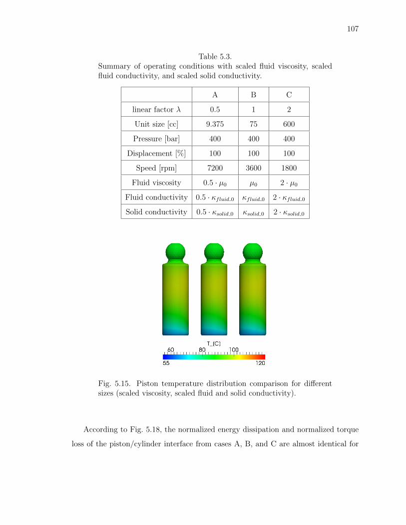
107

Table 5.3.Summary of operating conditions with scaled fluid viscosity, scaledfluid conductivity, and scaled solid conductivity.

A B C


Unit size [cc] 9.375 75 600



Speed [rpm] 7200 3600 1800

Fluid viscosity 0.5 · µ0 µ0 2 · µ0

Fluid conductivity 0.5 · κfluid 0 κfluid 0 2 · κfluid 0

Solid conductivity 0.5 · κsolid 0 κsolid 0 2 · κsolid 0

Fig. 5.15. Piston temperature distribution comparison for differentsizes (scaled viscosity, scaled fluid and solid conductivity).

According to Fig. 5.18, the normalized energy dissipation and normalized torque

loss of the piston/cylinder interface from cases A, B, and C are almost identical for

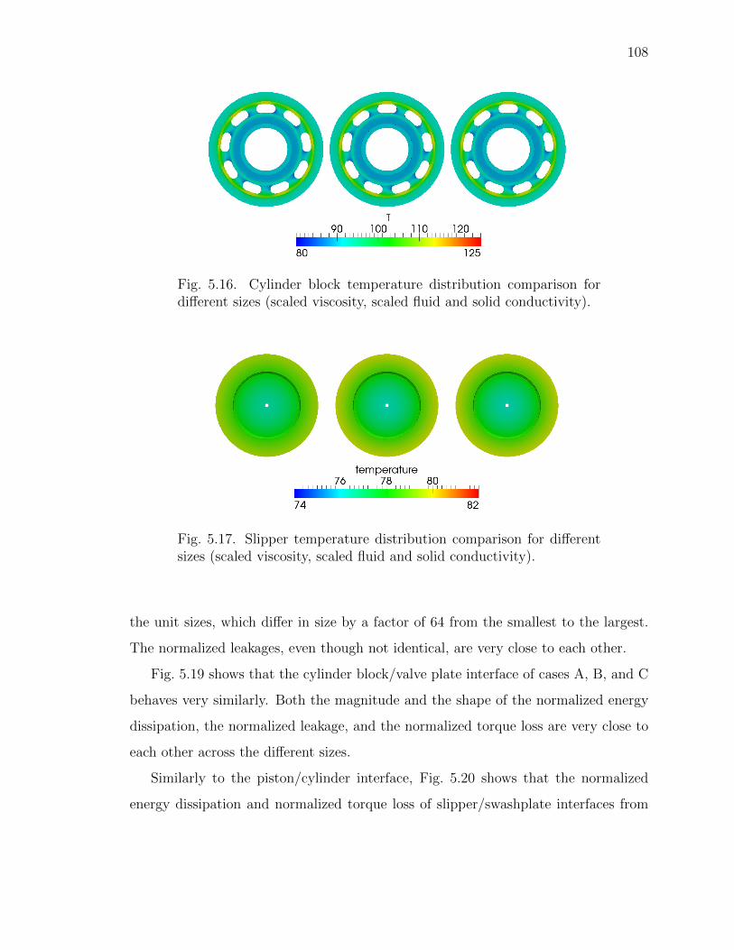
108

Fig. 5.16. Cylinder block temperature distribution comparison fordifferent sizes (scaled viscosity, scaled fluid and solid conductivity).

Fig. 5.17. Slipper temperature distribution comparison for differentsizes (scaled viscosity, scaled fluid and solid conductivity).

the unit sizes, which differ in size by a factor of 64 from the smallest to the largest.

The normalized leakages, even though not identical, are very close to each other.

Fig. 5.19 shows that the cylinder block/valve plate interface of cases A, B, and C

behaves very similarly. Both the magnitude and the shape of the normalized energy

dissipation, the normalized leakage, and the normalized torque loss are very close to

each other across the different sizes.

Similarly to the piston/cylinder interface, Fig. 5.20 shows that the normalized

energy dissipation and normalized torque loss of slipper/swashplate interfaces from

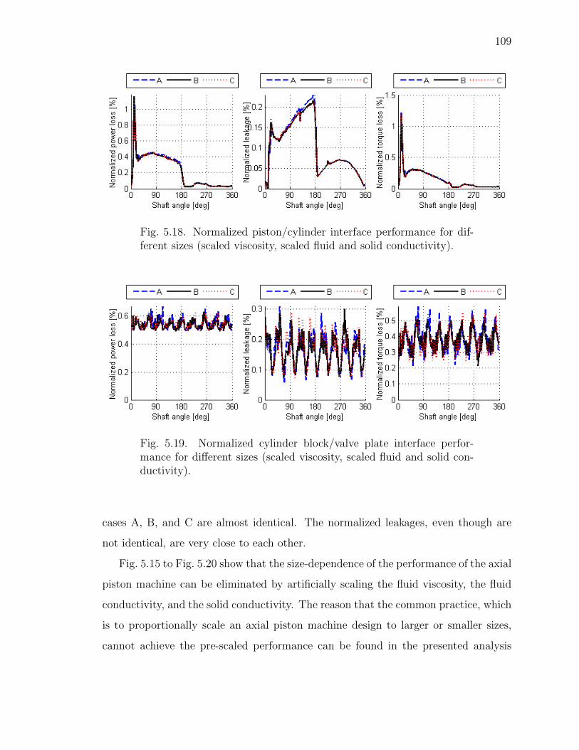
109

Fig. 5.18. Normalized piston/cylinder interface performance for dif-ferent sizes (scaled viscosity, scaled fluid and solid conductivity).

Fig. 5.19. Normalized cylinder block/valve plate interface perfor-mance for different sizes (scaled viscosity, scaled fluid and solid con-ductivity).

cases A, B, and C are almost identical. The normalized leakages, even though are

not identical, are very close to each other.

Fig. 5.15 to Fig. 5.20 show that the size-dependence of the performance of the axial

piston machine can be eliminated by artificially scaling the fluid viscosity, the fluid

conductivity, and the solid conductivity. The reason that the common practice, which

is to proportionally scale an axial piston machine design to larger or smaller sizes,

cannot achieve the pre-scaled performance can be found in the presented analysis

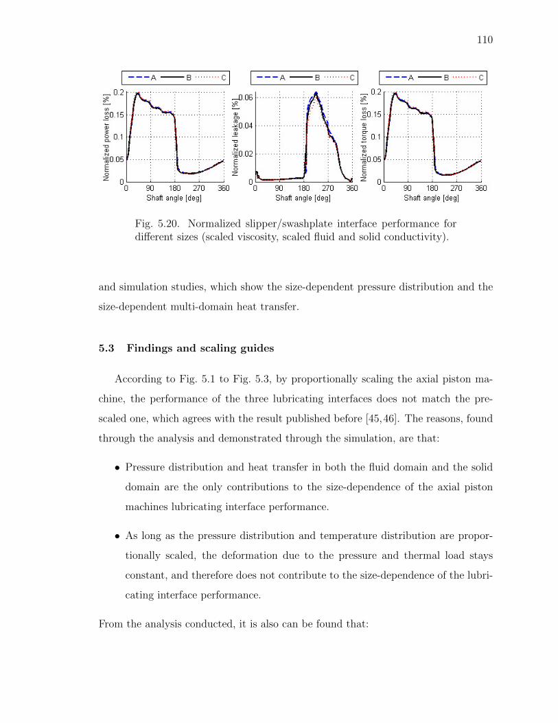
110

Fig. 5.20. Normalized slipper/swashplate interface performance fordifferent sizes (scaled viscosity, scaled fluid and solid conductivity).

and simulation studies, which show the size-dependent pressure distribution and the

size-dependent multi-domain heat transfer.

5.3 Findings and scaling guides

According to Fig. 5.1 to Fig. 5.3, by proportionally scaling the axial piston ma-

chine, the performance of the three lubricating interfaces does not match the pre-

scaled one, which agrees with the result published before [45,46]. The reasons, found

through the analysis and demonstrated through the simulation, are that:

• Pressure distribution and heat transfer in both the fluid domain and the solid

domain are the only contributions to the size-dependence of the axial piston

machines lubricating interface performance.

• As long as the pressure distribution and temperature distribution are propor-

tionally scaled, the deformation due to the pressure and thermal load stays

constant, and therefore does not contribute to the size-dependence of the lubri-

cating interface performance.

From the analysis conducted, it is also can be found that:

111

• A size-independent fluid pressure distribution can be achieved by scaling the

viscosity with the linear scaling factor. The simulation results in Fig. 5.5 to

Fig. 5.7 demonstrated this by showing an identical normalized performance for

all three lubricating interfaces when using a scaled viscosity and no heat transfer.

Since the viscosity can not be scaled artificially according to the linear scaling

factor in the real life, non-scalable viscosity contributes to the size-dependence

of the performance of lubricating interfaces.

• The size-independent temperature distribution in both the fluid and solid do-

mains can be achieved by scaling the fluid and solid conductivity with the linear

scaling factor. The simulation results in Fig. 5.15 to Fig. 5.20 demonstrated this

by showing an identical normalized performance for all three lubricating inter-

faces with a scaled viscosity and conductivity. Since the thermal conductivity

can not be scaled artificially according to the linear scaling factor in the real

life, non-scalable thermal behavior contributes to the size-dependence of the

performance of lubricating interfaces.

From the findings of the analysis and simulation studies, the following scaling guide

for all three lubricating interfaces emerges:

• When scaling an swashplate type axial piston machines to a different size, the

size-dependent pressure distribution-induced performance bias can be elimi-

nated by using hydraulic fluid at a different viscosity grade.

– Use higher viscosity for up-scaling.

– Use lower viscosity for down-scaling.

– Choose the viscosity based on the linear scaling factor as in Eq. 5.22.

• The viscosity of the fluid can also be controlled by:

– Increasing operating temperature for down-scaling

– Decreasing operating temperature for up-scaling.

112

• When using a fluid of different viscosity is not feasible, design modifications

should compensate for the size-dependent sealing function of the scaled lubri-

cating interfaces:

– For the piston/cylinder interface, use a lower normalized clearance for up-

scaling, and use a higher normalized clearance for down-scaling [46].

– For the cylinder block/valve plate interface, increase the sealing land area

for up-scaling, and decrease the sealing land area for down-scaling [45].

– For the slipper/swashplate interface, increase the sealing land area for up-

scaling, and decrease the sealing land area for down-scaling.

• To compensate for the size-dependent heat transfer, the design of the lubricating

interfaces needs to be modified:

– When up-scaling, the lubricating interface design should be modified to

increase the cooling performance of the lubricating gap, e.g. adding a flow

channel beneath the valve plate to smooth the temperature distribution.

– When down-scaling, the lubricating interface design should be modified to

create more thermal deformation, e.g. by using a bi-material solid body

[47].

Even though the simulation studies shown pertain to the fluid-structure and ther-

mal interaction model for all the three lubricating interfaces in a swashplate type

axial piston machine, the analytical study is not limited to a single type of hydraulic

pump. The findings will hold true for not only the tribological interfaces in axial pis-

ton machines, radial piston machines, internal and external gear pumps and motors,

gerotors, and vane pumps, but also for all the thermoelastohydrodynamic tribological

interfaces in bearings and seals.

113

5.4 Conclusions

This chapter presented an analytical study of the size-dependence of thermoelas-

tohydrodynamic tribological interfaces. The physical phenomena that were studied

include the hydrostatic and hydrodynamic pressure distributions, the heat transfer

and heat generation in the fluid film, the heat transfer in the solid domain, and the

solid body deformation due to both the pressure loading and the thermal loading.

The analysis indicates that the pressure distribution in the lubricating gap, and the

heat transfer in the fluid and in the solid bodies are the only size-dependent physical

phenomena; therefore, they are the only contributors to the performance change of

the thermoelastohydrodynamic tribological interfaces in response to scaling.

A state-of-the-art fluid-structure-thermal interaction model for the three lubricat-

ing interfaces in axial piston machines was used to demonstrate the consequences of

the analytical study. Three different pump sizes were modeled in a series of simulation

studies, the largest of which is 64 times bigger than the smallest. These simulation

studies verified the findings of the analysis, and allowed for the creation of a general

guide to scaling aimed at maintaining the efficiency of the original unit. This scaling

guide enables pump manufacturers to apply the developed scaling laws, and efficiently

generate scaled pump designs of much higher efficiency than the traditional approach

of linear scaling allows for.

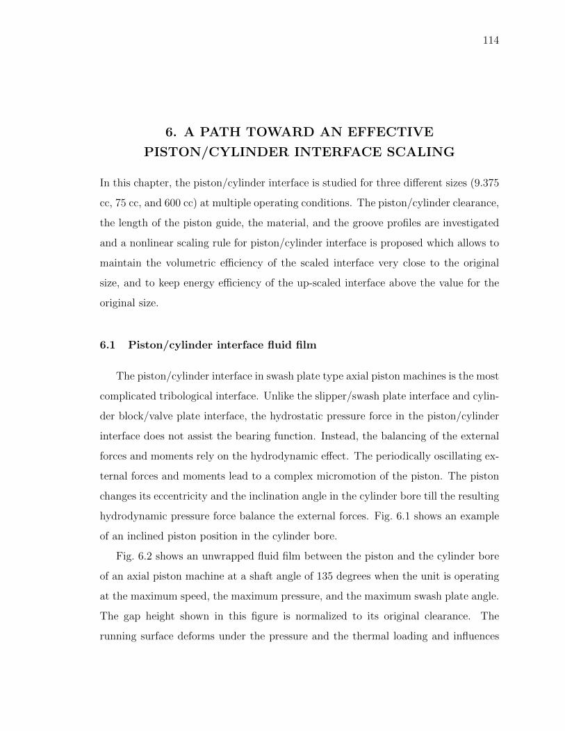
114

6. A PATH TOWARD AN EFFECTIVE

PISTON/CYLINDER INTERFACE SCALING

In this chapter, the piston/cylinder interface is studied for three different sizes (9.375

cc, 75 cc, and 600 cc) at multiple operating conditions. The piston/cylinder clearance,

the length of the piston guide, the material, and the groove profiles are investigated

and a nonlinear scaling rule for piston/cylinder interface is proposed which allows to

maintain the volumetric efficiency of the scaled interface very close to the original

size, and to keep energy efficiency of the up-scaled interface above the value for the

original size.

6.1 Piston/cylinder interface fluid film

The piston/cylinder interface in swash plate type axial piston machines is the most

complicated tribological interface. Unlike the slipper/swash plate interface and cylin-

der block/valve plate interface, the hydrostatic pressure force in the piston/cylinder

interface does not assist the bearing function. Instead, the balancing of the external

forces and moments rely on the hydrodynamic effect. The periodically oscillating ex-

ternal forces and moments lead to a complex micromotion of the piston. The piston

changes its eccentricity and the inclination angle in the cylinder bore till the resulting

hydrodynamic pressure force balance the external forces. Fig. 6.1 shows an example

of an inclined piston position in the cylinder bore.

Fig. 6.2 shows an unwrapped fluid film between the piston and the cylinder bore

of an axial piston machine at a shaft angle of 135 degrees when the unit is operating

at the maximum speed, the maximum pressure, and the maximum swash plate angle.

The gap height shown in this figure is normalized to its original clearance. The

running surface deforms under the pressure and the thermal loading and influences

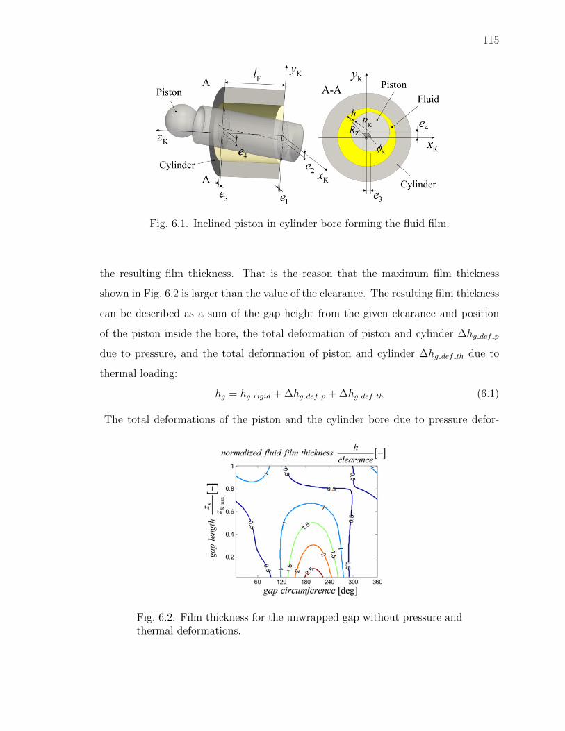
115

Fig. 6.1. Inclined piston in cylinder bore forming the fluid film.

the resulting film thickness. That is the reason that the maximum film thickness

shown in Fig. 6.2 is larger than the value of the clearance. The resulting film thickness

can be described as a sum of the gap height from the given clearance and position

of the piston inside the bore, the total deformation of piston and cylinder ∆hg def p

due to pressure, and the total deformation of piston and cylinder ∆hg def th due to

thermal loading:

hg = hg rigid + ∆hg def p + ∆hg def th (6.1)

The total deformations of the piston and the cylinder bore due to pressure defor-

Fig. 6.2. Film thickness for the unwrapped gap without pressure andthermal deformations.

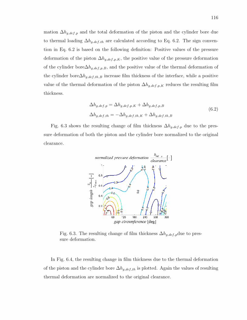
116

mation ∆hg def p and the total deformation of the piston and the cylinder bore due

to thermal loading ∆hg def th are calculated according to Eq. 6.2. The sign conven-

tion in Eq. 6.2 is based on the following definition: Positive values of the pressure

deformation of the piston ∆hg def p K , the positive value of the pressure deformation

of the cylinder bore∆hg def p B, and the positive value of the thermal deformation of

the cylinder bore∆hg def th B increase film thickness of the interface, while a positive

value of the thermal deformation of the piston ∆hg def p K reduces the resulting film

thickness.

∆hg def p = ∆hg def p K + ∆hg def p B

∆hg def th = −∆hg def th K + ∆hg def th B

(6.2)

Fig. 6.3 shows the resulting change of film thickness ∆hg def p due to the pres-

sure deformation of both the piston and the cylinder bore normalized to the original

clearance.

Fig. 6.3. The resulting change of film thickness ∆hg def pdue to pres-sure deformation.

In Fig. 6.4, the resulting change in film thickness due to the thermal deformation

of the piston and the cylinder bore ∆hg def th is plotted. Again the values of resulting

thermal deformation are normalized to the original clearance.

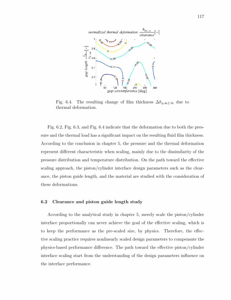
117

Fig. 6.4. The resulting change of film thickness ∆hg def th due tothermal deformation.

Fig. 6.2, Fig. 6.3, and Fig. 6.4 indicate that the deformation due to both the pres-

sure and the thermal load has a significant impact on the resulting fluid film thickness.

According to the conclusion in chapter 5, the pressure and the thermal deformation

represent different characteristic when scaling, mainly due to the dissimilarity of the

pressure distribution and temperature distribution. On the path toward the effective

scaling approach, the piston/cylinder interface design parameters such as the clear-

ance, the piston guide length, and the material are studied with the consideration of

these deformations.

6.2 Clearance and piston guide length study

According to the analytical study in chapter 5, merely scale the piston/cylinder

interface proportionally can never achieve the goal of the effective scaling, which is

to keep the performance as the pre-scaled size, by physics. Therefore, the effec-

tive scaling practice requires nonlinearly scaled design parameters to compensate the

physics-based performance difference. The path toward the effective piston/cylinder

interface scaling start from the understanding of the design parameters influence on

the interface performance.

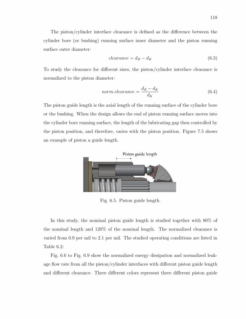
118

The piston/cylinder interface clearance is defined as the difference between the

cylinder bore (or bushing) running surface inner diameter and the piston running

surface outer diameter:

clearance = dB − dK (6.3)

To study the clearance for different sizes, the piston/cylinder interface clearance is

normalized to the piston diameter:

norm.clearance =dB − dKdK

(6.4)

The piston guide length is the axial length of the running surface of the cylinder bore

or the bushing. When the design allows the end of piston running surface moves into

the cylinder bore running surface, the length of the lubricating gap then controlled by

the piston position, and therefore, varies with the piston position. Figure 7.5 shows

an example of piston a guide length.

Fig. 6.5. Piston guide length.

In this study, the nominal piston guide length is studied together with 80% of

the nominal length and 120% of the nominal length. The normalized clearance is

varied from 0.9 per mil to 2.1 per mil. The studied operating conditions are listed in

Table 6.2:

Fig. 6.6 to Fig. 6.9 show the normalized energy dissipation and normalized leak-

age flow rate from all the piston/cylinder interfaces with different piston guide length

and different clearance. Three different colors represent three different piston guide

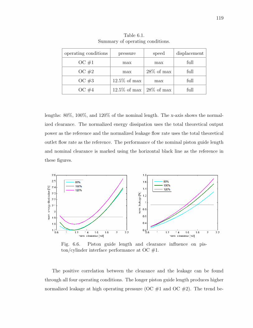
119

Table 6.1.Summary of operating conditions.

operating conditions pressure speed displacement

OC #1 max max full

OC #2 max 28% of max full

OC #3 12.5% of max max full

OC #4 12.5% of max 28% of max full

lengths: 80%, 100%, and 120% of the nominal length. The x-axis shows the normal-

ized clearance. The normalized energy dissipation uses the total theoretical output

power as the reference and the normalized leakage flow rate uses the total theoretical

outlet flow rate as the reference. The performance of the nominal piston guide length

and nominal clearance is marked using the horizontal black line as the reference in

these figures.

Fig. 6.6. Piston guide length and clearance influence on pis-ton/cylinder interface performance at OC #1.

The positive correlation between the clearance and the leakage can be found

through all four operating conditions. The longer piston guide length produces higher

normalized leakage at high operating pressure (OC #1 and OC #2). The trend be-

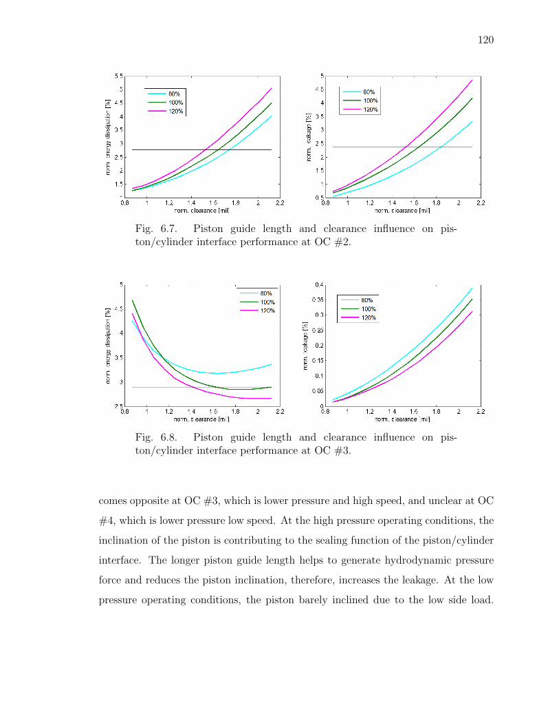
120



comes opposite at OC #3, which is lower pressure and high speed, and unclear at OC

#4, which is lower pressure low speed. At the high pressure operating conditions, the

inclination of the piston is contributing to the sealing function of the piston/cylinder

interface. The longer piston guide length helps to generate hydrodynamic pressure

force and reduces the piston inclination, therefore, increases the leakage. At the low

pressure operating conditions, the piston barely inclined due to the low side load.

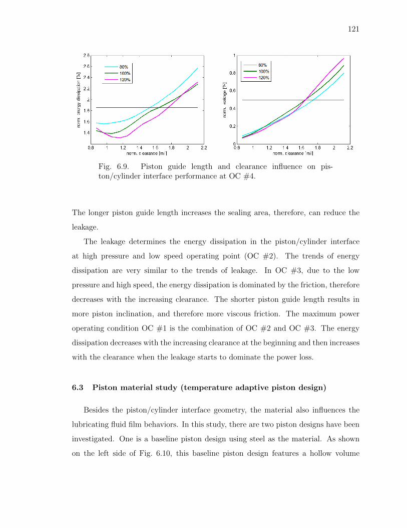
121


The longer piston guide length increases the sealing area, therefore, can reduce the

leakage.

The leakage determines the energy dissipation in the piston/cylinder interface

at high pressure and low speed operating point (OC #2). The trends of energy

dissipation are very similar to the trends of leakage. In OC #3, due to the low

pressure and high speed, the energy dissipation is dominated by the friction, therefore

decreases with the increasing clearance. The shorter piston guide length results in

more piston inclination, and therefore more viscous friction. The maximum power

operating condition OC #1 is the combination of OC #2 and OC #3. The energy

dissipation decreases with the increasing clearance at the beginning and then increases

with the clearance when the leakage starts to dominate the power loss.

6.3 Piston material study (temperature adaptive piston design)

Besides the piston/cylinder interface geometry, the material also influences the

lubricating fluid film behaviors. In this study, there are two piston designs have been

investigated. One is a baseline piston design using steel as the material. As shown

on the left side of Fig. 6.10, this baseline piston design features a hollow volume

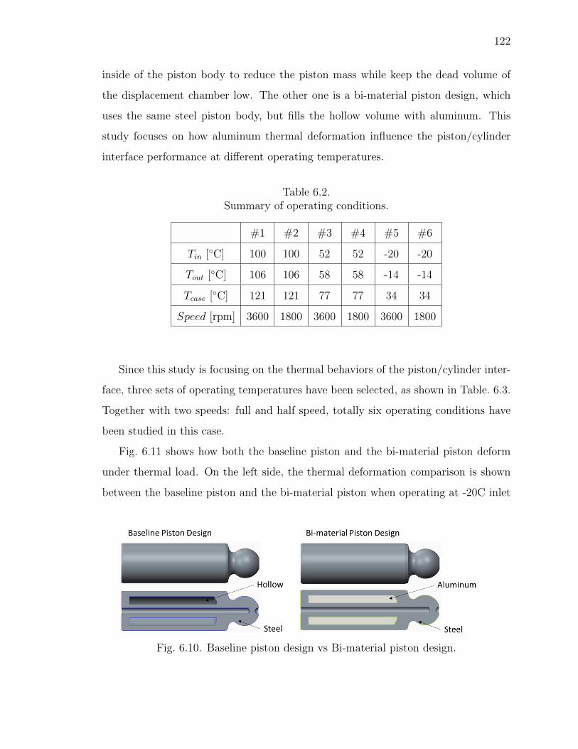
122

inside of the piston body to reduce the piston mass while keep the dead volume of

the displacement chamber low. The other one is a bi-material piston design, which

uses the same steel piston body, but fills the hollow volume with aluminum. This

study focuses on how aluminum thermal deformation influence the piston/cylinder

interface performance at different operating temperatures.

Table 6.2.Summary of operating conditions.

#1 #2 #3 #4 #5 #6

Tin [◦C] 100 100 52 52 -20 -20

Tout [◦C] 106 106 58 58 -14 -14

Tcase [◦C] 121 121 77 77 34 34

Speed [rpm] 3600 1800 3600 1800 3600 1800

Since this study is focusing on the thermal behaviors of the piston/cylinder inter-

face, three sets of operating temperatures have been selected, as shown in Table. 6.3.

Together with two speeds: full and half speed, totally six operating conditions have

been studied in this case.

Fig. 6.11 shows how both the baseline piston and the bi-material piston deform

under thermal load. On the left side, the thermal deformation comparison is shown

between the baseline piston and the bi-material piston when operating at -20C inlet

Fig. 6.10. Baseline piston design vs Bi-material piston design.

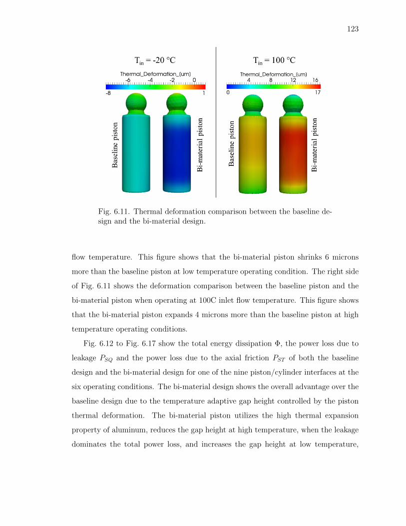
123

Fig. 6.11. Thermal deformation comparison between the baseline de-sign and the bi-material design.

flow temperature. This figure shows that the bi-material piston shrinks 6 microns

more than the baseline piston at low temperature operating condition. The right side

of Fig. 6.11 shows the deformation comparison between the baseline piston and the

bi-material piston when operating at 100C inlet flow temperature. This figure shows

that the bi-material piston expands 4 microns more than the baseline piston at high

temperature operating conditions.

Fig. 6.12 to Fig. 6.17 show the total energy dissipation Φ, the power loss due to

leakage PSQ and the power loss due to the axial friction PST of both the baseline

design and the bi-material design for one of the nine piston/cylinder interfaces at the

six operating conditions. The bi-material design shows the overall advantage over the

baseline design due to the temperature adaptive gap height controlled by the piston

thermal deformation. The bi-material piston utilizes the high thermal expansion

property of aluminum, reduces the gap height at high temperature, when the leakage

dominates the total power loss, and increases the gap height at low temperature,

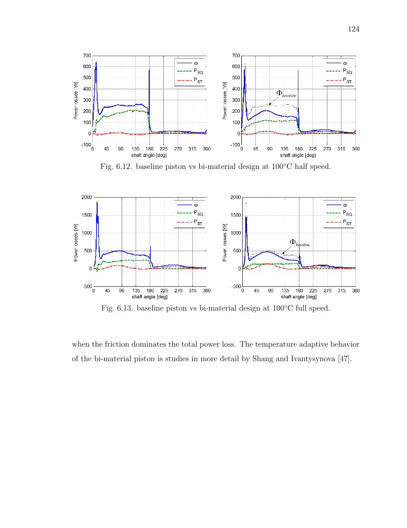
124

Fig. 6.12. baseline piston vs bi-material design at 100◦C half speed.

Fig. 6.13. baseline piston vs bi-material design at 100◦C full speed.

when the friction dominates the total power loss. The temperature adaptive behavior

of the bi-material piston is studies in more detail by Shang and Ivantysynova [47].

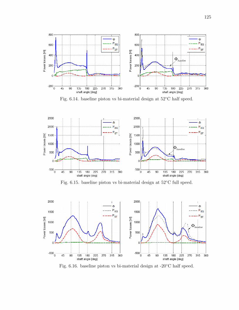
125

Fig. 6.14. baseline piston vs bi-material design at 52◦C half speed.

Fig. 6.15. baseline piston vs bi-material design at 52◦C full speed.

Fig. 6.16. baseline piston vs bi-material design at -20◦C half speed.

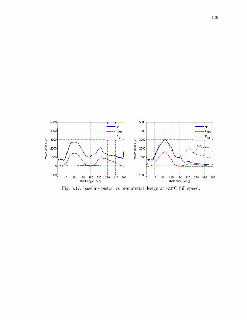
126

Fig. 6.17. baseline piston vs bi-material design at -20◦C full speed.

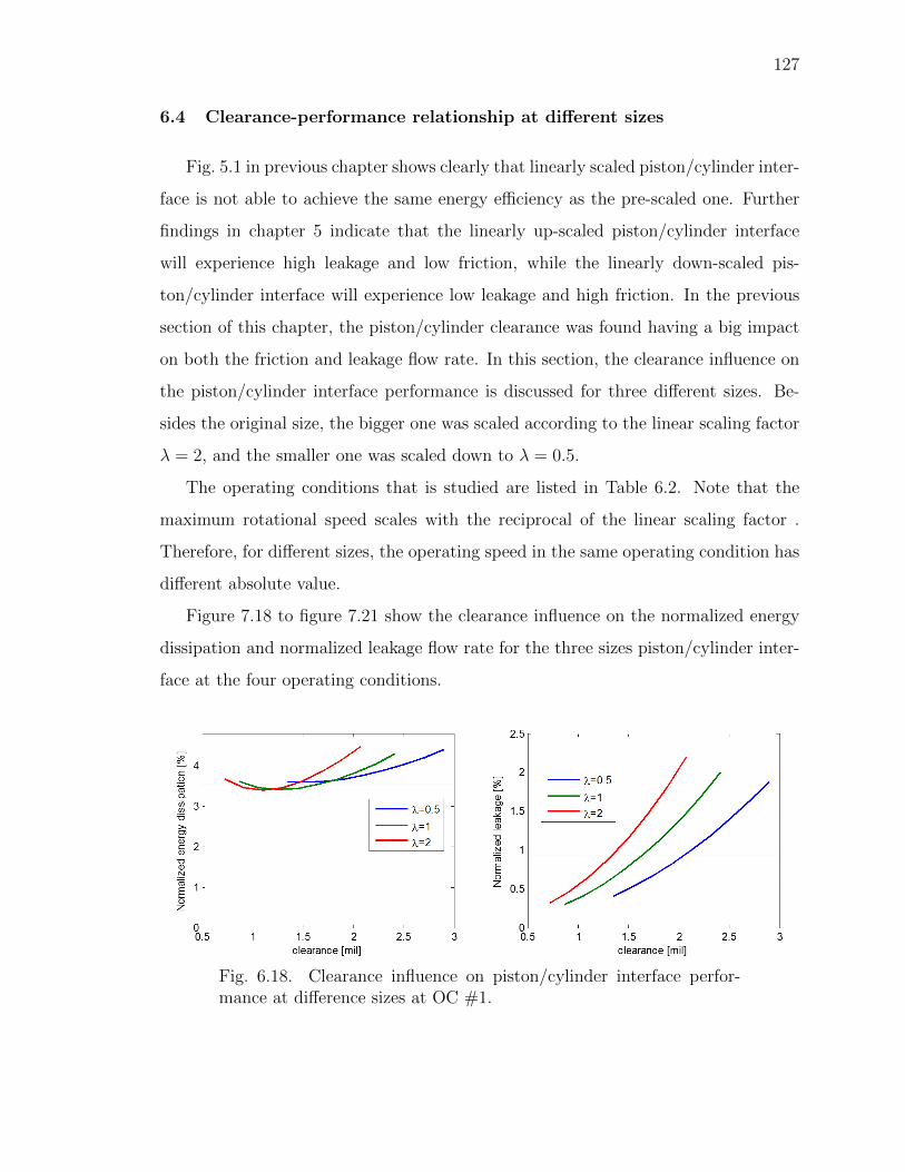
127

6.4 Clearance-performance relationship at different sizes

Fig. 5.1 in previous chapter shows clearly that linearly scaled piston/cylinder inter-

face is not able to achieve the same energy efficiency as the pre-scaled one. Further

findings in chapter 5 indicate that the linearly up-scaled piston/cylinder interface

will experience high leakage and low friction, while the linearly down-scaled pis-

ton/cylinder interface will experience low leakage and high friction. In the previous

section of this chapter, the piston/cylinder clearance was found having a big impact

on both the friction and leakage flow rate. In this section, the clearance influence on

the piston/cylinder interface performance is discussed for three different sizes. Be-

sides the original size, the bigger one was scaled according to the linear scaling factor

λ = 2, and the smaller one was scaled down to λ = 0.5.

The operating conditions that is studied are listed in Table 6.2. Note that the

maximum rotational speed scales with the reciprocal of the linear scaling factor .

Therefore, for different sizes, the operating speed in the same operating condition has

different absolute value.

Figure 7.18 to figure 7.21 show the clearance influence on the normalized energy

dissipation and normalized leakage flow rate for the three sizes piston/cylinder inter-

face at the four operating conditions.

Fig. 6.18. Clearance influence on piston/cylinder interface perfor-mance at difference sizes at OC #1.

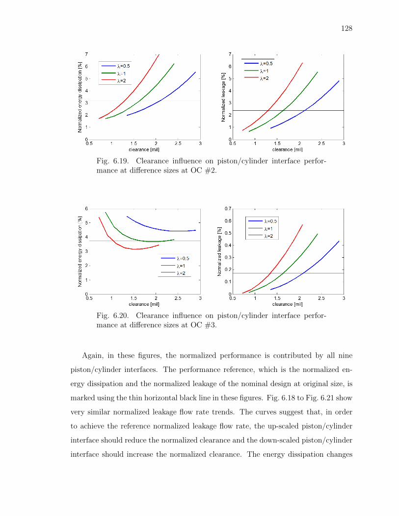
128



Again, in these figures, the normalized performance is contributed by all nine

piston/cylinder interfaces. The performance reference, which is the normalized en-

ergy dissipation and the normalized leakage of the nominal design at original size, is

marked using the thin horizontal black line in these figures. Fig. 6.18 to Fig. 6.21 show

very similar normalized leakage flow rate trends. The curves suggest that, in order

to achieve the reference normalized leakage flow rate, the up-scaled piston/cylinder

interface should reduce the normalized clearance and the down-scaled piston/cylinder

interface should increase the normalized clearance. The energy dissipation changes

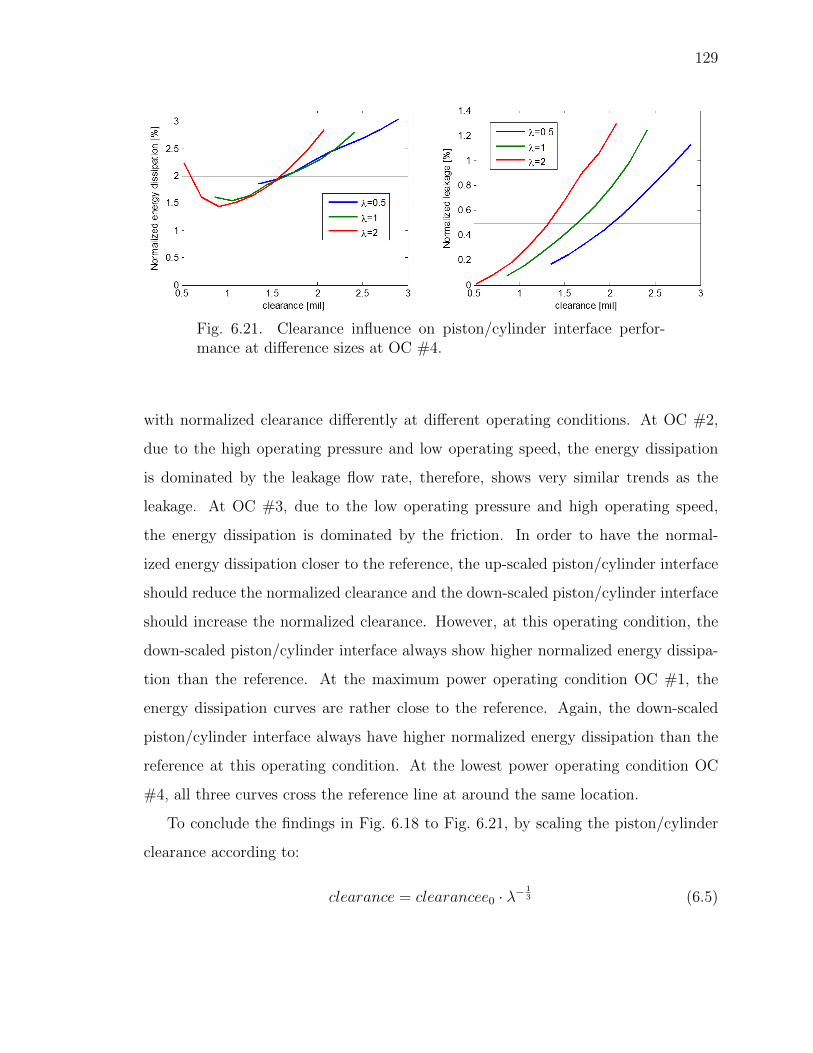
129


with normalized clearance differently at different operating conditions. At OC #2,

due to the high operating pressure and low operating speed, the energy dissipation

is dominated by the leakage flow rate, therefore, shows very similar trends as the

leakage. At OC #3, due to the low operating pressure and high operating speed,

the energy dissipation is dominated by the friction. In order to have the normal-

ized energy dissipation closer to the reference, the up-scaled piston/cylinder interface

should reduce the normalized clearance and the down-scaled piston/cylinder interface

should increase the normalized clearance. However, at this operating condition, the

down-scaled piston/cylinder interface always show higher normalized energy dissipa-

tion than the reference. At the maximum power operating condition OC #1, the

energy dissipation curves are rather close to the reference. Again, the down-scaled

piston/cylinder interface always have higher normalized energy dissipation than the

reference at this operating condition. At the lowest power operating condition OC

#4, all three curves cross the reference line at around the same location.

To conclude the findings in Fig. 6.18 to Fig. 6.21, by scaling the piston/cylinder

clearance according to:

clearance = clearancee0 · λ−13 (6.5)

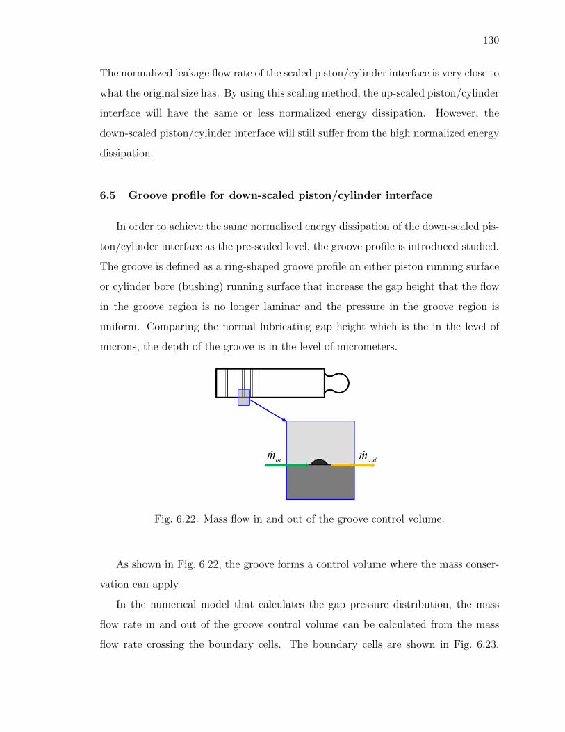
130

The normalized leakage flow rate of the scaled piston/cylinder interface is very close to

what the original size has. By using this scaling method, the up-scaled piston/cylinder

interface will have the same or less normalized energy dissipation. However, the

down-scaled piston/cylinder interface will still suffer from the high normalized energy

dissipation.

6.5 Groove profile for down-scaled piston/cylinder interface

In order to achieve the same normalized energy dissipation of the down-scaled pis-

ton/cylinder interface as the pre-scaled level, the groove profile is introduced studied.

The groove is defined as a ring-shaped groove profile on either piston running surface

or cylinder bore (bushing) running surface that increase the gap height that the flow

in the groove region is no longer laminar and the pressure in the groove region is

uniform. Comparing the normal lubricating gap height which is the in the level of

microns, the depth of the groove is in the level of micrometers.

Fig. 6.22. Mass flow in and out of the groove control volume.

As shown in Fig. 6.22, the groove forms a control volume where the mass conser-

vation can apply.

In the numerical model that calculates the gap pressure distribution, the mass

flow rate in and out of the groove control volume can be calculated from the mass

flow rate crossing the boundary cells. The boundary cells are shown in Fig. 6.23.

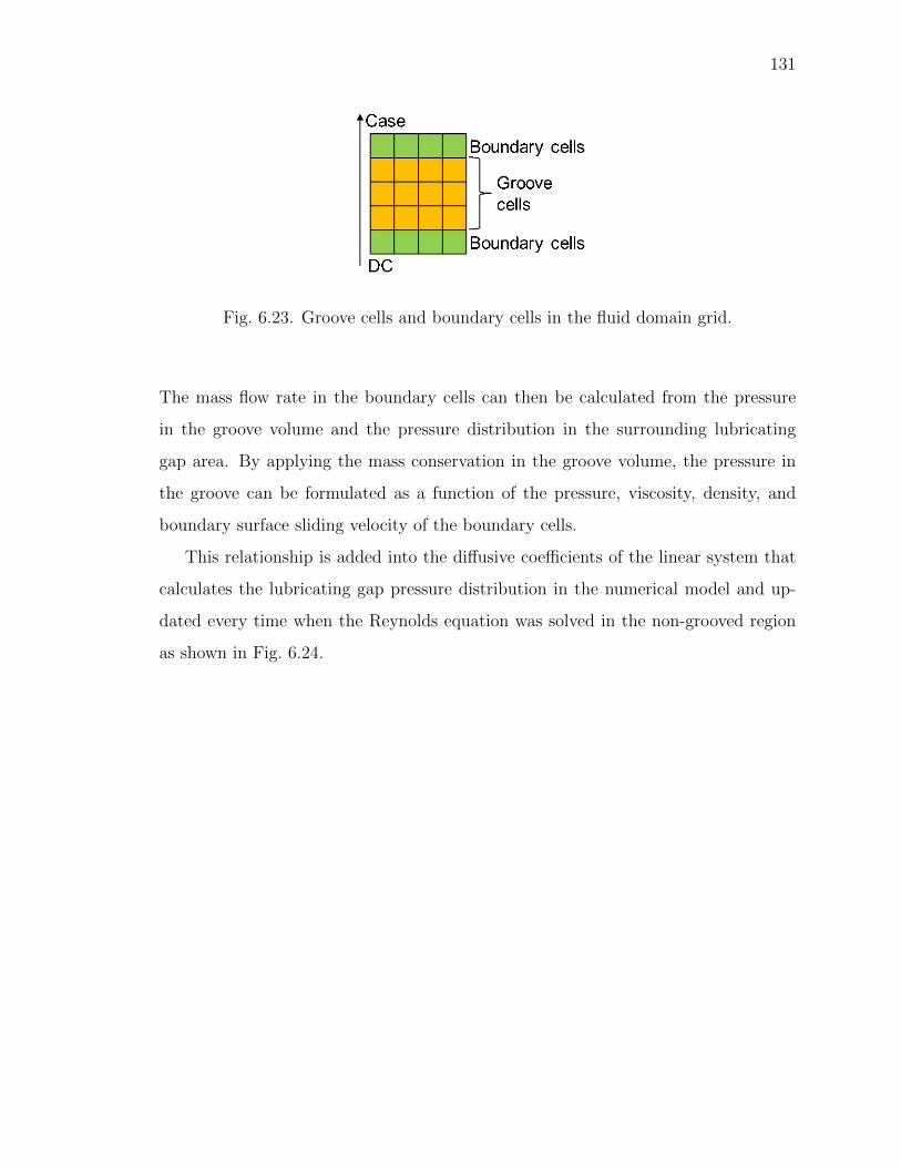
131

Fig. 6.23. Groove cells and boundary cells in the fluid domain grid.

The mass flow rate in the boundary cells can then be calculated from the pressure

in the groove volume and the pressure distribution in the surrounding lubricating

gap area. By applying the mass conservation in the groove volume, the pressure in

the groove can be formulated as a function of the pressure, viscosity, density, and

boundary surface sliding velocity of the boundary cells.

This relationship is added into the diffusive coefficients of the linear system that

calculates the lubricating gap pressure distribution in the numerical model and up-

dated every time when the Reynolds equation was solved in the non-grooved region

as shown in Fig. 6.24.

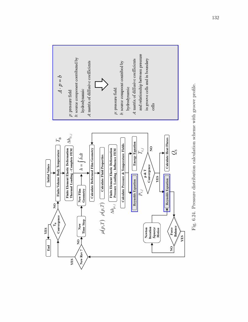
132

Fig

.6.

24.

Pre

ssure

dis

trib

uti

onca

lcula

tion

schem

ew

ith

groov

epro

file

.

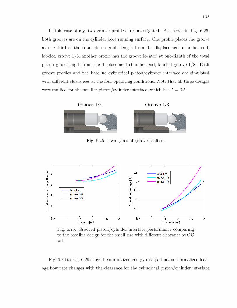
133

In this case study, two groove profiles are investigated. As shown in Fig. 6.25,

both grooves are on the cylinder bore running surface. One profile places the groove

at one-third of the total piston guide length from the displacement chamber end,

labeled groove 1/3, another profile has the groove located at one-eighth of the total

piston guide length from the displacement chamber end, labeled groove 1/8. Both

groove profiles and the baseline cylindrical piston/cylinder interface are simulated

with different clearances at the four operating conditions. Note that all three designs

were studied for the smaller piston/cylinder interface, which has λ = 0.5.

Fig. 6.25. Two types of groove profiles.

Fig. 6.26. Grooved piston/cylinder interface performance comparingto the baseline design for the small size with different clearance at OC#1.

Fig. 6.26 to Fig. 6.29 show the normalized energy dissipation and normalized leak-

age flow rate changes with the clearance for the cylindrical piston/cylinder interface

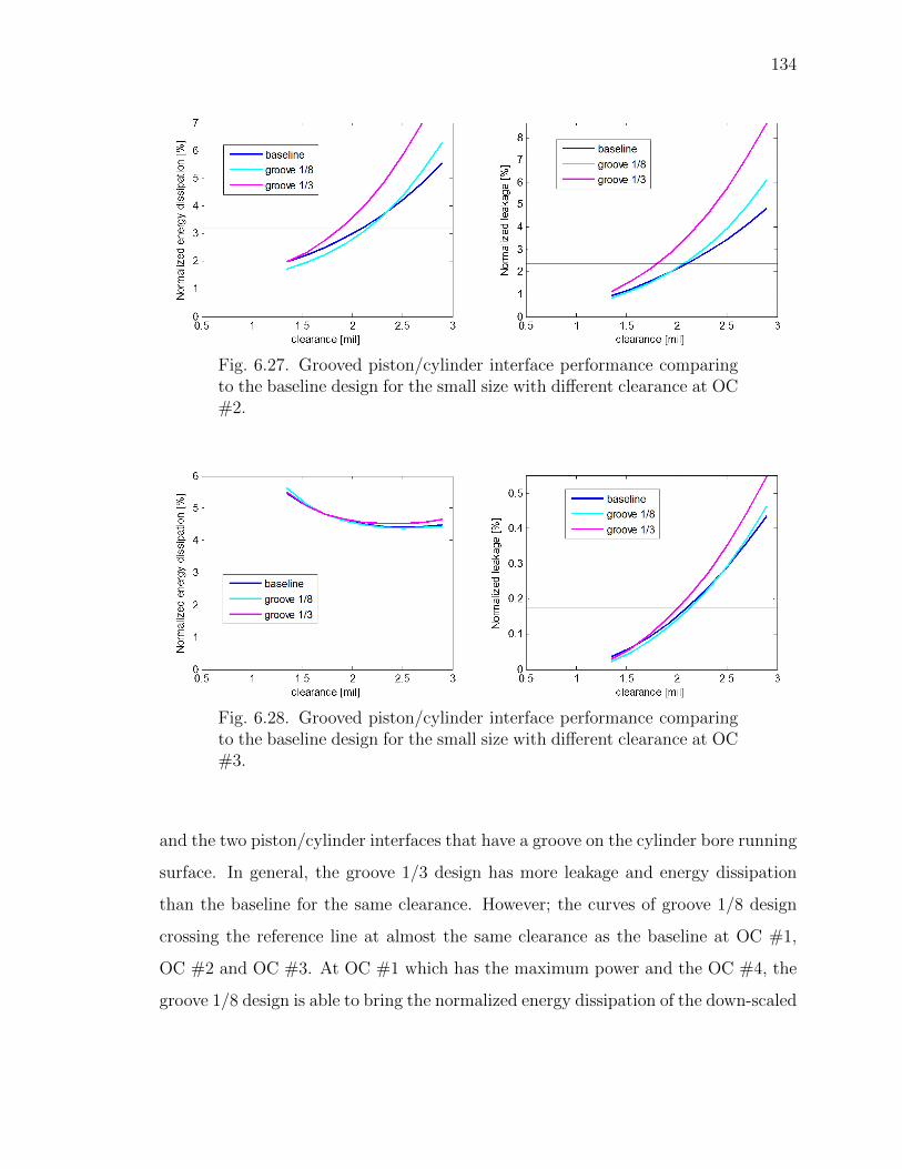
134



and the two piston/cylinder interfaces that have a groove on the cylinder bore running

surface. In general, the groove 1/3 design has more leakage and energy dissipation

than the baseline for the same clearance. However; the curves of groove 1/8 design

crossing the reference line at almost the same clearance as the baseline at OC #1,

OC #2 and OC #3. At OC #1 which has the maximum power and the OC #4, the

groove 1/8 design is able to bring the normalized energy dissipation of the down-scaled

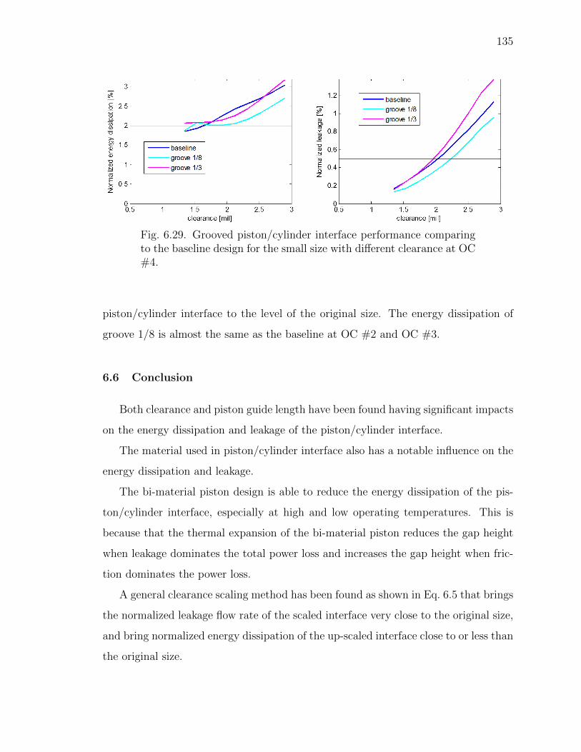
135


piston/cylinder interface to the level of the original size. The energy dissipation of

groove 1/8 is almost the same as the baseline at OC #2 and OC #3.

6.6 Conclusion

Both clearance and piston guide length have been found having significant impacts

on the energy dissipation and leakage of the piston/cylinder interface.

The material used in piston/cylinder interface also has a notable influence on the

energy dissipation and leakage.

The bi-material piston design is able to reduce the energy dissipation of the pis-

ton/cylinder interface, especially at high and low operating temperatures. This is

because that the thermal expansion of the bi-material piston reduces the gap height

when leakage dominates the total power loss and increases the gap height when fric-

tion dominates the power loss.

A general clearance scaling method has been found as shown in Eq. 6.5 that brings

the normalized leakage flow rate of the scaled interface very close to the original size,

and bring normalized energy dissipation of the up-scaled interface close to or less than

the original size.

136

The groove profile on the cylinder bore surface located one-eighth of the piston

guide length from the displacement chamber end is able to bring the normalized

energy dissipation of the down-scaled piston/cylinder interface to the value of the

original size at maximum and minimum power operating conditions.

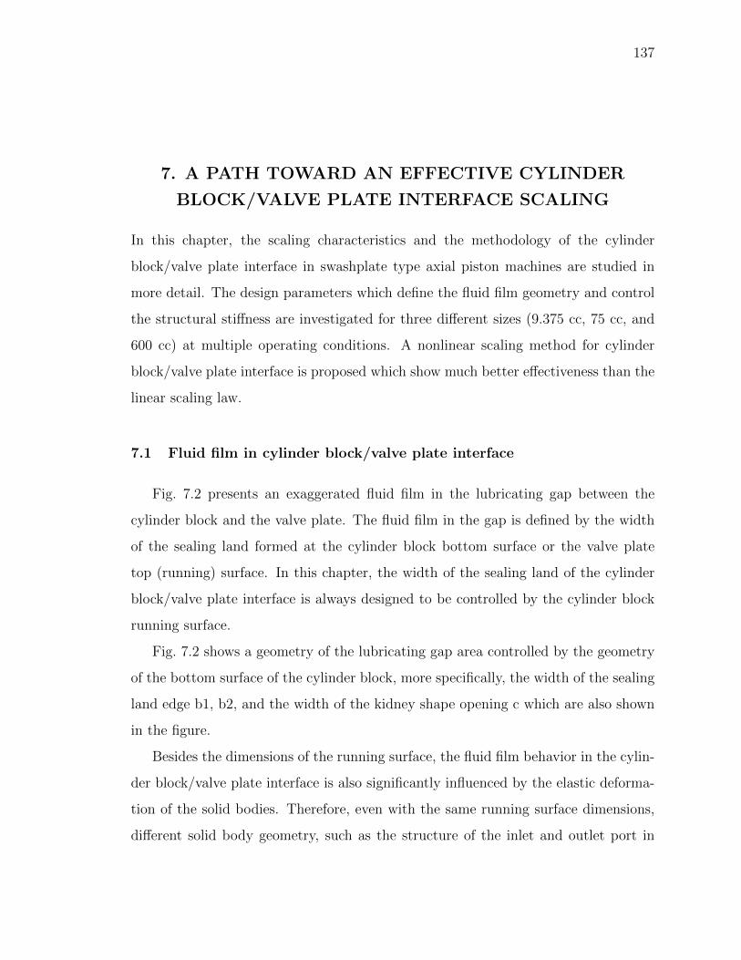
137

7. A PATH TOWARD AN EFFECTIVE CYLINDER

BLOCK/VALVE PLATE INTERFACE SCALING

In this chapter, the scaling characteristics and the methodology of the cylinder

block/valve plate interface in swashplate type axial piston machines are studied in

more detail. The design parameters which define the fluid film geometry and control

the structural stiffness are investigated for three different sizes (9.375 cc, 75 cc, and

600 cc) at multiple operating conditions. A nonlinear scaling method for cylinder

block/valve plate interface is proposed which show much better effectiveness than the

linear scaling law.

7.1 Fluid film in cylinder block/valve plate interface

Fig. 7.2 presents an exaggerated fluid film in the lubricating gap between the

cylinder block and the valve plate. The fluid film in the gap is defined by the width

of the sealing land formed at the cylinder block bottom surface or the valve plate

top (running) surface. In this chapter, the width of the sealing land of the cylinder

block/valve plate interface is always designed to be controlled by the cylinder block

running surface.

Fig. 7.2 shows a geometry of the lubricating gap area controlled by the geometry

of the bottom surface of the cylinder block, more specifically, the width of the sealing

land edge b1, b2, and the width of the kidney shape opening c which are also shown

in the figure.

Besides the dimensions of the running surface, the fluid film behavior in the cylin-

der block/valve plate interface is also significantly influenced by the elastic deforma-

tion of the solid bodies. Therefore, even with the same running surface dimensions,

different solid body geometry, such as the structure of the inlet and outlet port in

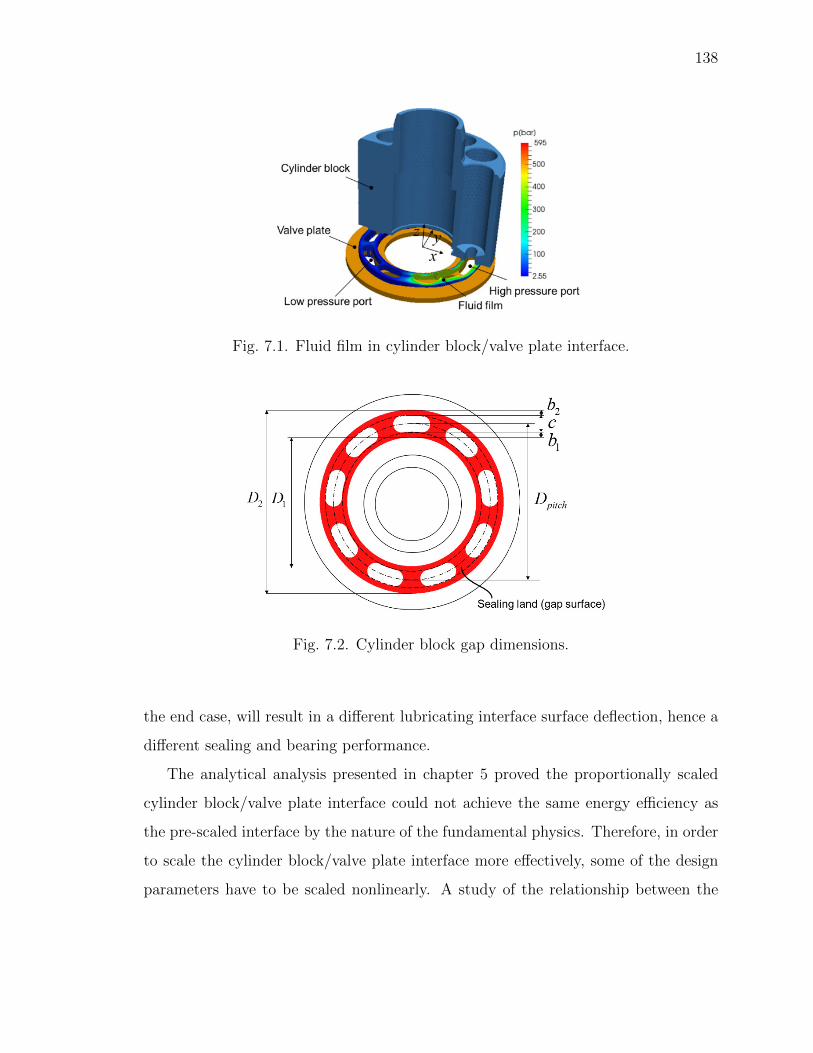
138

Fig. 7.1. Fluid film in cylinder block/valve plate interface.

Fig. 7.2. Cylinder block gap dimensions.

the end case, will result in a different lubricating interface surface deflection, hence a

different sealing and bearing performance.

The analytical analysis presented in chapter 5 proved the proportionally scaled

cylinder block/valve plate interface could not achieve the same energy efficiency as

the pre-scaled interface by the nature of the fundamental physics. Therefore, in order

to scale the cylinder block/valve plate interface more effectively, some of the design

parameters have to be scaled nonlinearly. A study of the relationship between the

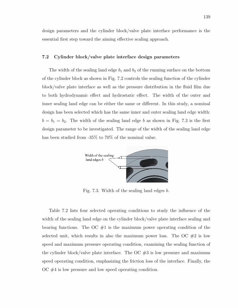
139

design parameters and the cylinder block/valve plate interface performance is the

essential first step toward the aiming effective scaling approach.

7.2 Cylinder block/valve plate interface design parameters

The width of the sealing land edge b1 and b2 of the running surface on the bottom

of the cylinder block as shown in Fig. 7.2 controls the sealing function of the cylinder

block/valve plate interface as well as the pressure distribution in the fluid film due

to both hydrodynamic effect and hydrostatic effect. The width of the outer and

inner sealing land edge can be either the same or different. In this study, a nominal

design has been selected which has the same inner and outer sealing land edge width:

b = b1 = b2. The width of the sealing land edge b as shown in Fig. 7.3 is the first

design parameter to be investigated. The range of the width of the sealing land edge

has been studied from -35% to 70% of the nominal value.

Fig. 7.3. Width of the sealing land edges b.

Table 7.2 lists four selected operating conditions to study the influence of the

width of the sealing land edge on the cylinder block/valve plate interface sealing and

bearing functions. The OC #1 is the maximum power operating condition of the

selected unit, which results in also the maximum power loss. The OC #2 is low

speed and maximum pressure operating condition, examining the sealing function of

the cylinder block/valve plate interface. The OC #3 is low pressure and maximum

speed operating condition, emphasizing the friction loss of the interface. Finally, the

OC #4 is low pressure and low speed operating condition.

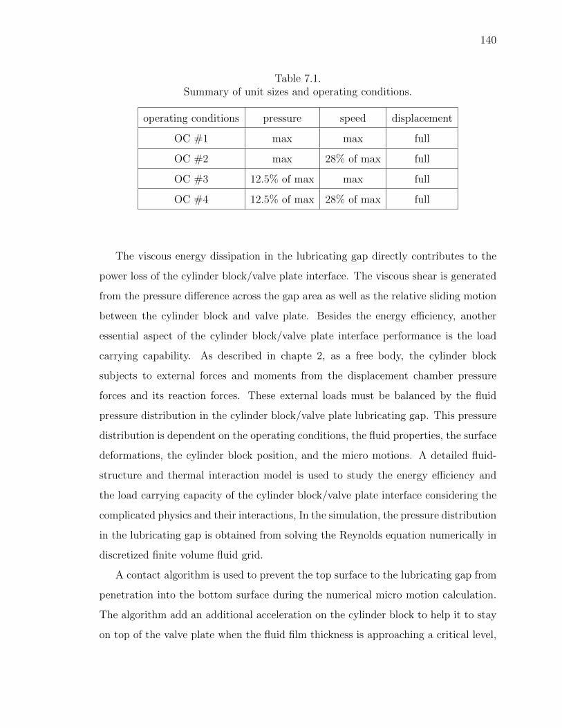
140



OC #1 max max full




The viscous energy dissipation in the lubricating gap directly contributes to the

power loss of the cylinder block/valve plate interface. The viscous shear is generated

from the pressure difference across the gap area as well as the relative sliding motion

between the cylinder block and valve plate. Besides the energy efficiency, another

essential aspect of the cylinder block/valve plate interface performance is the load

carrying capability. As described in chapte 2, as a free body, the cylinder block

subjects to external forces and moments from the displacement chamber pressure

forces and its reaction forces. These external loads must be balanced by the fluid

pressure distribution in the cylinder block/valve plate lubricating gap. This pressure

distribution is dependent on the operating conditions, the fluid properties, the surface

deformations, the cylinder block position, and the micro motions. A detailed fluid-

structure and thermal interaction model is used to study the energy efficiency and

the load carrying capacity of the cylinder block/valve plate interface considering the

complicated physics and their interactions, In the simulation, the pressure distribution

in the lubricating gap is obtained from solving the Reynolds equation numerically in

discretized finite volume fluid grid.

A contact algorithm is used to prevent the top surface to the lubricating gap from

penetration into the bottom surface during the numerical micro motion calculation.

The algorithm add an additional acceleration on the cylinder block to help it to stay

on top of the valve plate when the fluid film thickness is approaching a critical level,

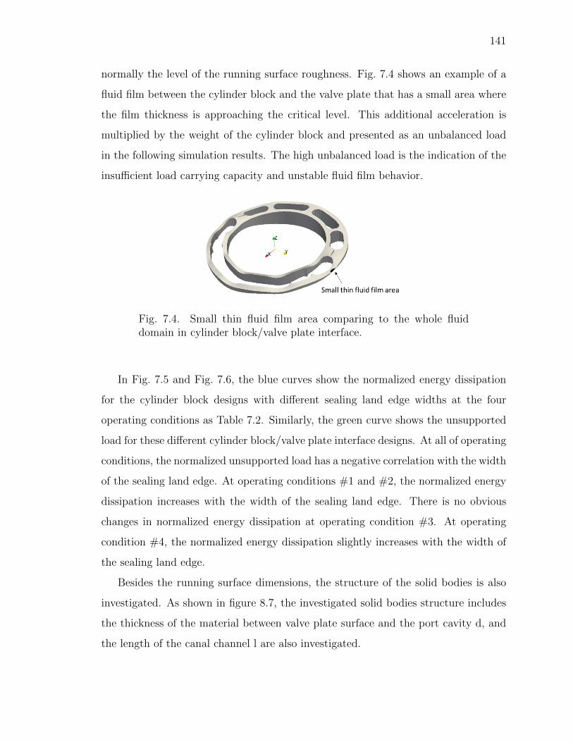
141

normally the level of the running surface roughness. Fig. 7.4 shows an example of a

fluid film between the cylinder block and the valve plate that has a small area where

the film thickness is approaching the critical level. This additional acceleration is

multiplied by the weight of the cylinder block and presented as an unbalanced load

in the following simulation results. The high unbalanced load is the indication of the

insufficient load carrying capacity and unstable fluid film behavior.

Fig. 7.4. Small thin fluid film area comparing to the whole fluiddomain in cylinder block/valve plate interface.

In Fig. 7.5 and Fig. 7.6, the blue curves show the normalized energy dissipation

for the cylinder block designs with different sealing land edge widths at the four

operating conditions as Table 7.2. Similarly, the green curve shows the unsupported

load for these different cylinder block/valve plate interface designs. At all of operating

conditions, the normalized unsupported load has a negative correlation with the width

of the sealing land edge. At operating conditions #1 and #2, the normalized energy

dissipation increases with the width of the sealing land edge. There is no obvious

changes in normalized energy dissipation at operating condition #3. At operating

condition #4, the normalized energy dissipation slightly increases with the width of

the sealing land edge.

Besides the running surface dimensions, the structure of the solid bodies is also

investigated. As shown in figure 8.7, the investigated solid bodies structure includes

the thickness of the material between valve plate surface and the port cavity d, and

the length of the canal channel l are also investigated.

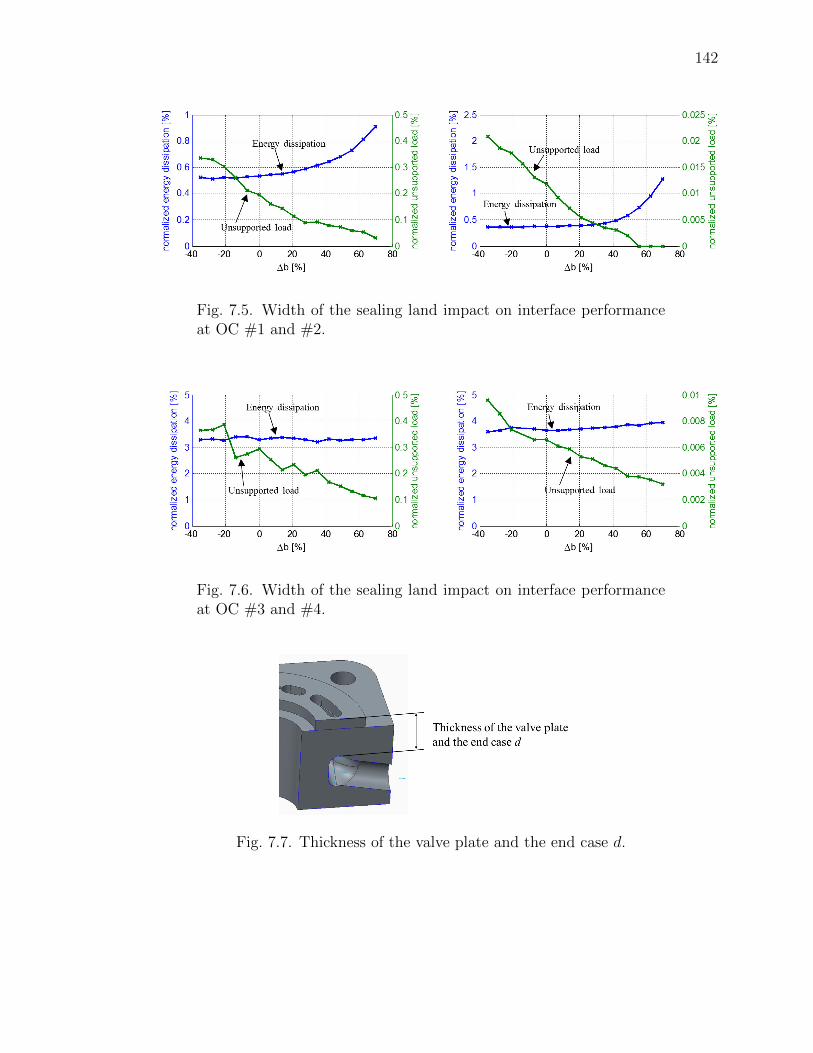
142

Fig. 7.5. Width of the sealing land impact on interface performanceat OC #1 and #2.

Fig. 7.6. Width of the sealing land impact on interface performanceat OC #3 and #4.

Fig. 7.7. Thickness of the valve plate and the end case d.

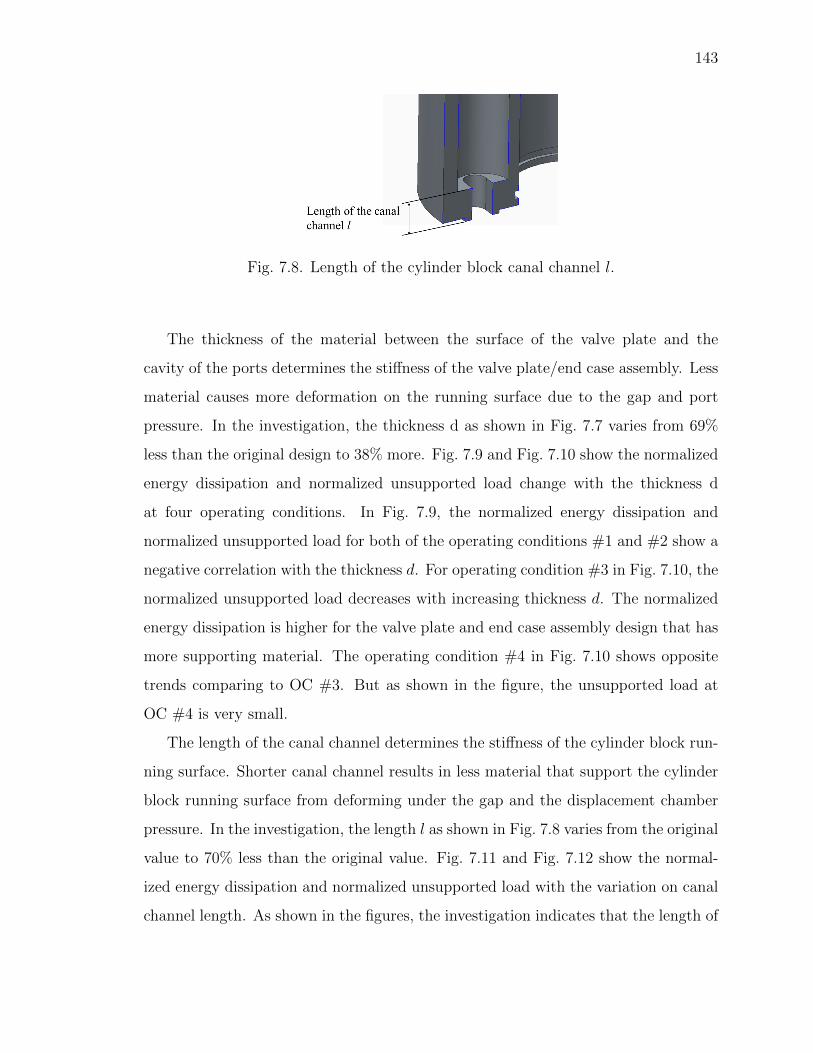
143

Fig. 7.8. Length of the cylinder block canal channel l.

The thickness of the material between the surface of the valve plate and the

cavity of the ports determines the stiffness of the valve plate/end case assembly. Less

material causes more deformation on the running surface due to the gap and port

pressure. In the investigation, the thickness d as shown in Fig. 7.7 varies from 69%

less than the original design to 38% more. Fig. 7.9 and Fig. 7.10 show the normalized

energy dissipation and normalized unsupported load change with the thickness d

at four operating conditions. In Fig. 7.9, the normalized energy dissipation and

normalized unsupported load for both of the operating conditions #1 and #2 show a

negative correlation with the thickness d. For operating condition #3 in Fig. 7.10, the

normalized unsupported load decreases with increasing thickness d. The normalized

energy dissipation is higher for the valve plate and end case assembly design that has

more supporting material. The operating condition #4 in Fig. 7.10 shows opposite

trends comparing to OC #3. But as shown in the figure, the unsupported load at

OC #4 is very small.

The length of the canal channel determines the stiffness of the cylinder block run-

ning surface. Shorter canal channel results in less material that support the cylinder

block running surface from deforming under the gap and the displacement chamber

pressure. In the investigation, the length l as shown in Fig. 7.8 varies from the original

value to 70% less than the original value. Fig. 7.11 and Fig. 7.12 show the normal-

ized energy dissipation and normalized unsupported load with the variation on canal

channel length. As shown in the figures, the investigation indicates that the length of

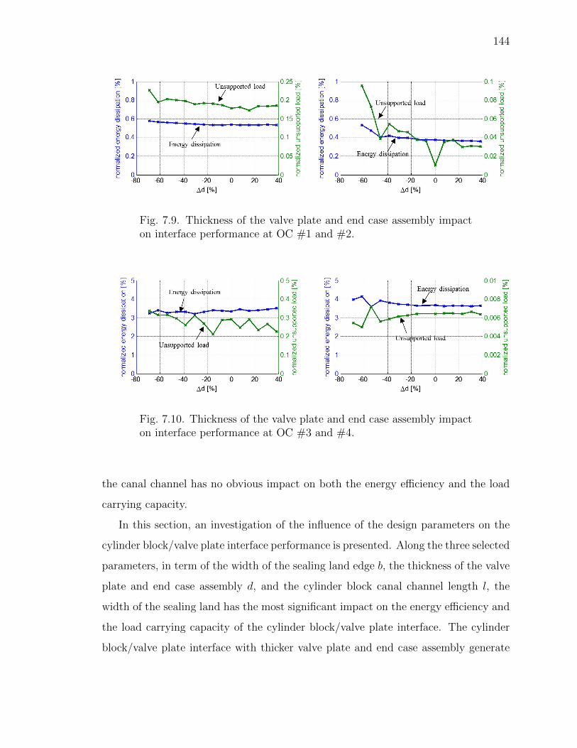
144

Fig. 7.9. Thickness of the valve plate and end case assembly impacton interface performance at OC #1 and #2.

Fig. 7.10. Thickness of the valve plate and end case assembly impacton interface performance at OC #3 and #4.

the canal channel has no obvious impact on both the energy efficiency and the load

carrying capacity.

In this section, an investigation of the influence of the design parameters on the

cylinder block/valve plate interface performance is presented. Along the three selected

parameters, in term of the width of the sealing land edge b, the thickness of the valve

plate and end case assembly d, and the cylinder block canal channel length l, the

width of the sealing land has the most significant impact on the energy efficiency and

the load carrying capacity of the cylinder block/valve plate interface. The cylinder

block/valve plate interface with thicker valve plate and end case assembly generate

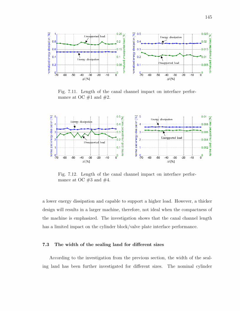
145

Fig. 7.11. Length of the canal channel impact on interface perfor-mance at OC #1 and #2.

Fig. 7.12. Length of the canal channel impact on interface perfor-mance at OC #3 and #4.

a lower energy dissipation and capable to support a higher load. However, a thicker

design will results in a larger machine, therefore, not ideal when the compactness of

the machine is emphasized. The investigation shows that the canal channel length

has a limited impact on the cylinder block/valve plate interface performance.

7.3 The width of the sealing land for different sizes

According to the investigation from the previous section, the width of the seal-

ing land has been further investigated for different sizes. The nominal cylinder

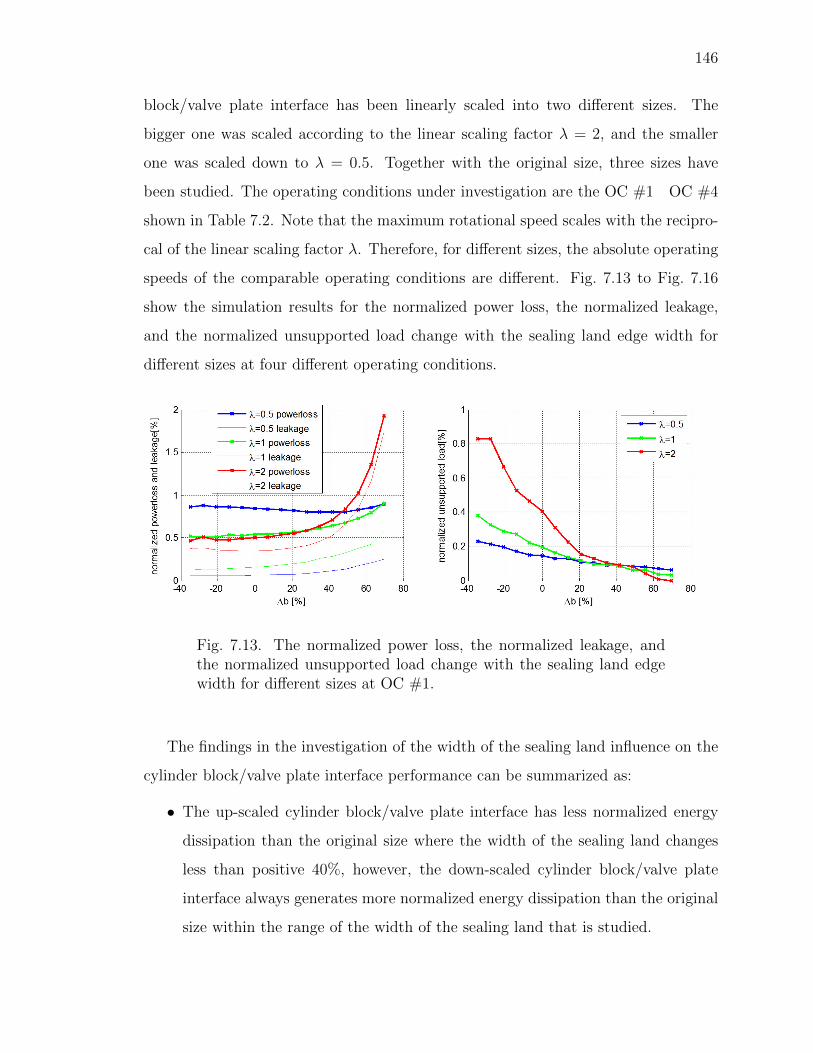
146

block/valve plate interface has been linearly scaled into two different sizes. The

bigger one was scaled according to the linear scaling factor λ = 2, and the smaller

one was scaled down to λ = 0.5. Together with the original size, three sizes have

been studied. The operating conditions under investigation are the OC #1 OC #4

shown in Table 7.2. Note that the maximum rotational speed scales with the recipro-

cal of the linear scaling factor λ. Therefore, for different sizes, the absolute operating

speeds of the comparable operating conditions are different. Fig. 7.13 to Fig. 7.16

show the simulation results for the normalized power loss, the normalized leakage,

and the normalized unsupported load change with the sealing land edge width for

different sizes at four different operating conditions.

Fig. 7.13. The normalized power loss, the normalized leakage, andthe normalized unsupported load change with the sealing land edgewidth for different sizes at OC #1.

The findings in the investigation of the width of the sealing land influence on the

cylinder block/valve plate interface performance can be summarized as:

• The up-scaled cylinder block/valve plate interface has less normalized energy

dissipation than the original size where the width of the sealing land changes

less than positive 40%, however, the down-scaled cylinder block/valve plate

interface always generates more normalized energy dissipation than the original

size within the range of the width of the sealing land that is studied.

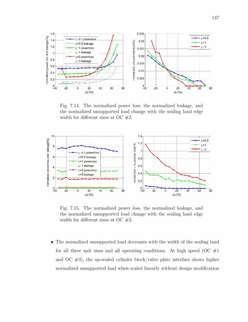
147



• The normalized unsupported load decreases with the width of the sealing land

for all three unit sizes and all operating conditions. At high speed (OC #1

and OC #3), the up-scaled cylinder block/valve plate interface shows higher

normalized unsupported load when scaled linearly without design modification

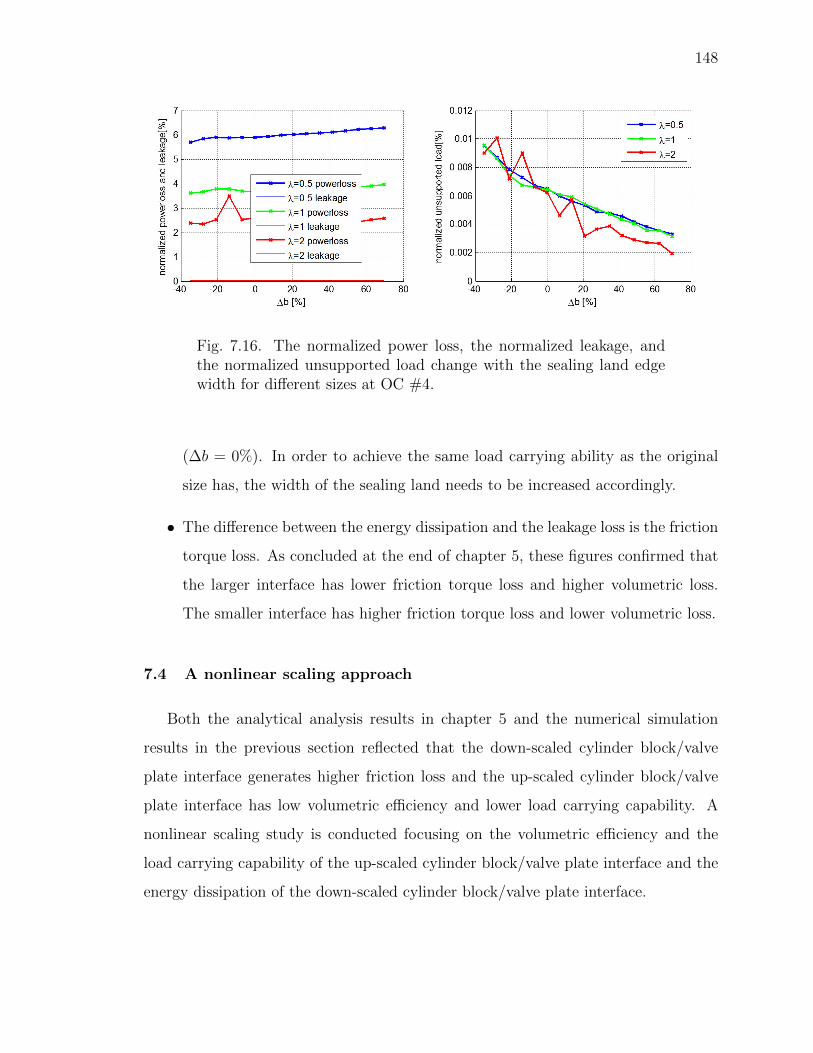
148


(∆b = 0%). In order to achieve the same load carrying ability as the original

size has, the width of the sealing land needs to be increased accordingly.

• The difference between the energy dissipation and the leakage loss is the friction

torque loss. As concluded at the end of chapter 5, these figures confirmed that

the larger interface has lower friction torque loss and higher volumetric loss.

The smaller interface has higher friction torque loss and lower volumetric loss.

7.4 A nonlinear scaling approach

Both the analytical analysis results in chapter 5 and the numerical simulation

results in the previous section reflected that the down-scaled cylinder block/valve

plate interface generates higher friction loss and the up-scaled cylinder block/valve

plate interface has low volumetric efficiency and lower load carrying capability. A

nonlinear scaling study is conducted focusing on the volumetric efficiency and the

load carrying capability of the up-scaled cylinder block/valve plate interface and the

energy dissipation of the down-scaled cylinder block/valve plate interface.

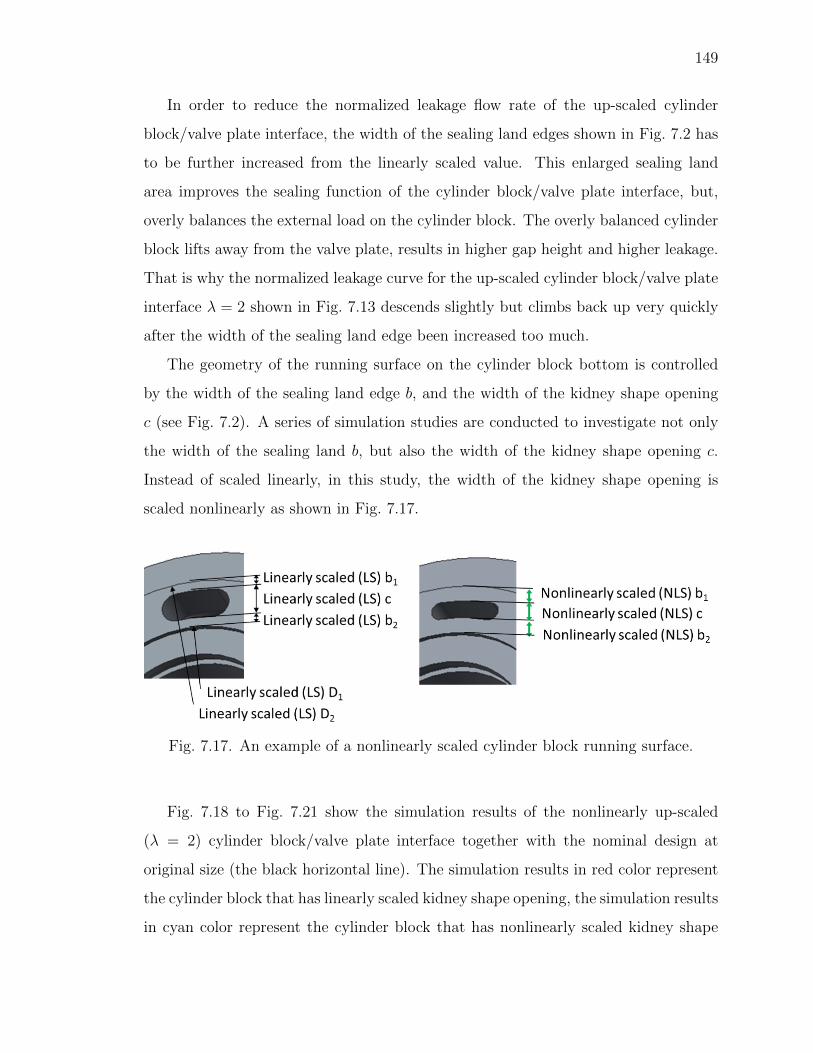
149

In order to reduce the normalized leakage flow rate of the up-scaled cylinder

block/valve plate interface, the width of the sealing land edges shown in Fig. 7.2 has

to be further increased from the linearly scaled value. This enlarged sealing land

area improves the sealing function of the cylinder block/valve plate interface, but,

overly balances the external load on the cylinder block. The overly balanced cylinder

block lifts away from the valve plate, results in higher gap height and higher leakage.

That is why the normalized leakage curve for the up-scaled cylinder block/valve plate

interface λ = 2 shown in Fig. 7.13 descends slightly but climbs back up very quickly

after the width of the sealing land edge been increased too much.

The geometry of the running surface on the cylinder block bottom is controlled

by the width of the sealing land edge b, and the width of the kidney shape opening

c (see Fig. 7.2). A series of simulation studies are conducted to investigate not only

the width of the sealing land b, but also the width of the kidney shape opening c.

Instead of scaled linearly, in this study, the width of the kidney shape opening is

scaled nonlinearly as shown in Fig. 7.17.

Fig. 7.17. An example of a nonlinearly scaled cylinder block running surface.

Fig. 7.18 to Fig. 7.21 show the simulation results of the nonlinearly up-scaled

(λ = 2) cylinder block/valve plate interface together with the nominal design at

original size (the black horizontal line). The simulation results in red color represent

the cylinder block that has linearly scaled kidney shape opening, the simulation results

in cyan color represent the cylinder block that has nonlinearly scaled kidney shape

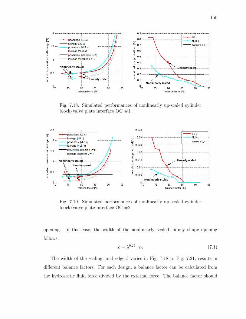
150

Fig. 7.18. Simulated performances of nonlinearly up-scaled cylinderblock/valve plate interface OC #1.


opening. In this case, the width of the nonlinearly scaled kidney shape opening

follows:

c = λ0.25 · c0 (7.1)

The width of the sealing land edge b varies in Fig. 7.18 to Fig. 7.21, results in

different balance factors. For each design, a balance factor can be calculated from

the hydrostatic fluid force divided by the external force. The balance factor should

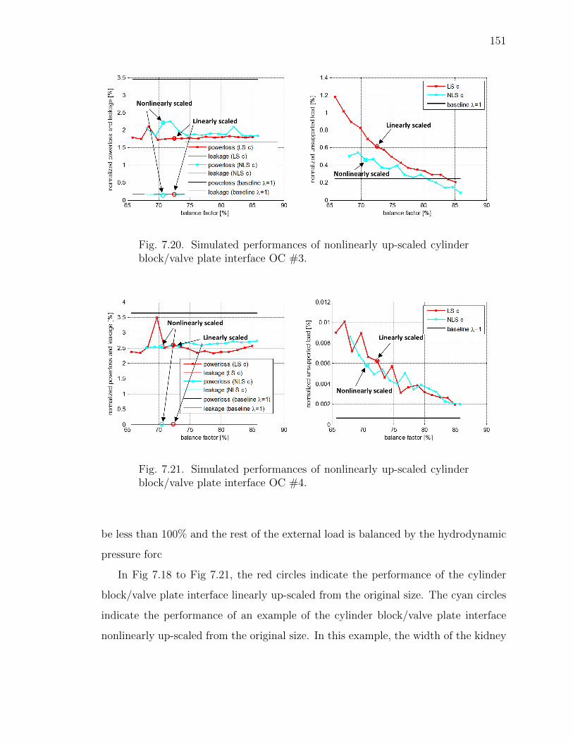
151



be less than 100% and the rest of the external load is balanced by the hydrodynamic

pressure forc

In Fig 7.18 to Fig 7.21, the red circles indicate the performance of the cylinder

block/valve plate interface linearly up-scaled from the original size. The cyan circles

indicate the performance of an example of the cylinder block/valve plate interface

nonlinearly up-scaled from the original size. In this example, the width of the kidney

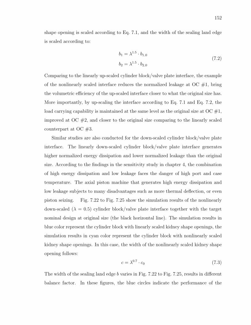
152

shape opening is scaled according to Eq. 7.1, and the width of the sealing land edge

is scaled according to:

b1 = λ1.5 · b1 0

b2 = λ1.5 · b2 0

(7.2)

Comparing to the linearly up-scaled cylinder block/valve plate interface, the example

of the nonlinearly scaled interface reduces the normalized leakage at OC #1, bring

the volumetric efficiency of the up-scaled interface closer to what the original size has.

More importantly, by up-scaling the interface according to Eq. 7.1 and Eq. 7.2, the

load carrying capability is maintained at the same level as the original size at OC #1,

improved at OC #2, and closer to the original size comparing to the linearly scaled

counterpart at OC #3.

Similar studies are also conducted for the down-scaled cylinder block/valve plate

interface. The linearly down-scaled cylinder block/valve plate interface generates

higher normalized energy dissipation and lower normalized leakage than the original

size. According to the findings in the sensitivity study in chapter 4, the combination

of high energy dissipation and low leakage faces the danger of high port and case

temperature. The axial piston machine that generates high energy dissipation and

low leakage subjects to many disadvantages such as more thermal deflection, or even

piston seizing. Fig. 7.22 to Fig. 7.25 show the simulation results of the nonlinearly

down-scaled (λ = 0.5) cylinder block/valve plate interface together with the target

nominal design at original size (the black horizontal line). The simulation results in

blue color represent the cylinder block with linearly scaled kidney shape openings, the

simulation results in cyan color represent the cylinder block with nonlinearly scaled

kidney shape openings. In this case, the width of the nonlinearly scaled kidney shape

opening follows:

c = λ0.7 · c0 (7.3)

The width of the sealing land edge b varies in Fig. 7.22 to Fig. 7.25, results in different

balance factor. In these figures, the blue circles indicate the performance of the

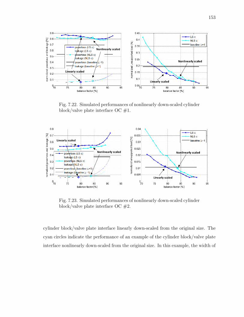
153

Fig. 7.22. Simulated performances of nonlinearly down-scaled cylinderblock/valve plate interface OC #1.


cylinder block/valve plate interface linearly down-scaled from the original size. The

cyan circles indicate the performance of an example of the cylinder block/valve plate

interface nonlinearly down-scaled from the original size. In this example, the width of

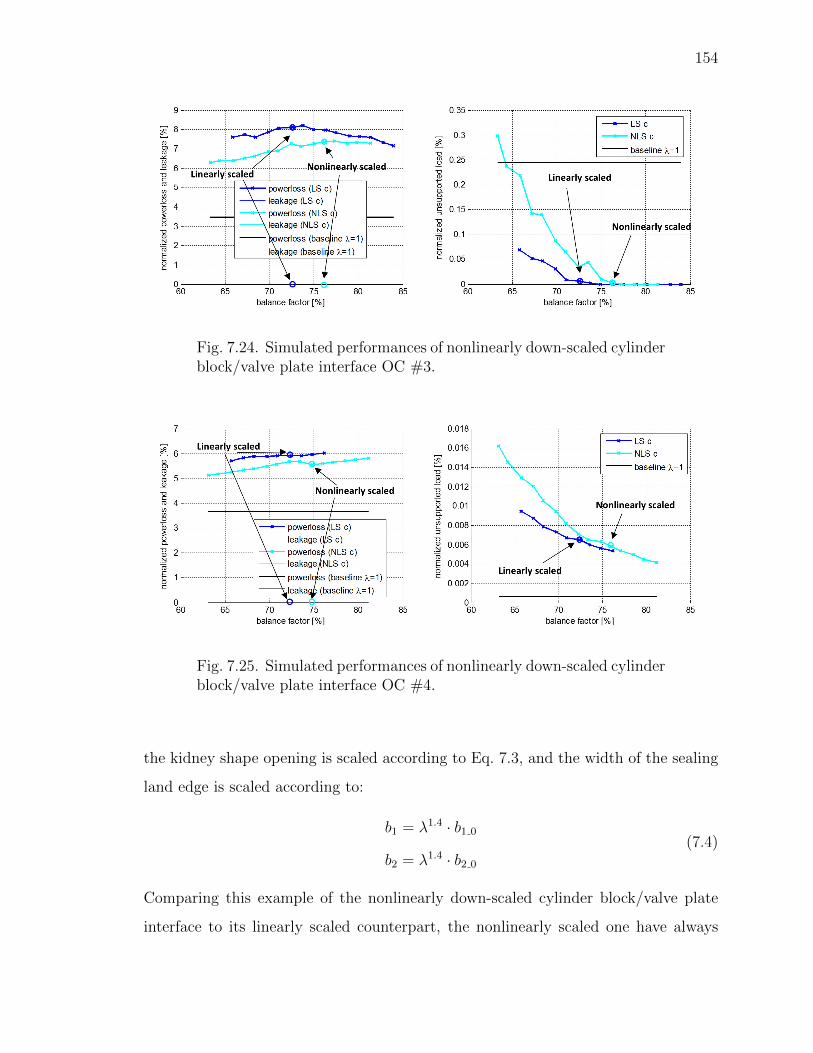
154



the kidney shape opening is scaled according to Eq. 7.3, and the width of the sealing

land edge is scaled according to:

b1 = λ1.4 · b1 0

b2 = λ1.4 · b2 0

(7.4)

Comparing this example of the nonlinearly down-scaled cylinder block/valve plate

interface to its linearly scaled counterpart, the nonlinearly scaled one have always

155

better load carrying capability. At all the operating conditions, the normalized energy

dissipation of the nonlinearly scaled cylinder block/valve plate interface is lower than

the linearly scaled one. At operating conditions #1 and #2, the nonlinearly scaled

interface also has the normalized leakage flow rate closer to the value of the reference.

7.5 Conclusion

The findings in this chapter can be summarized as:

• Both the width of the sealing land b and the thickness of the valve plate and

end case assembly d have significant impact on the performance of the cylinder

block/valve plate interface.

• Linearly scaled cylinder block/valve plate interface is not able to achieve the

energy efficiency and load carrying capacity as the pre-scaled interface.

• The proposed nonlinear scaling method is able to bring the performance and

the efficiency of the scaled interface closer to the original size.

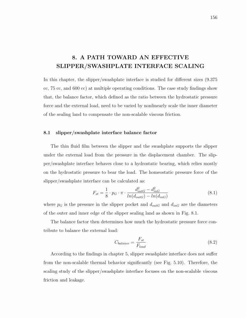
156

8. A PATH TOWARD AN EFFECTIVE

SLIPPER/SWASHPLATE INTERFACE SCALING

In this chapter, the slipper/swashplate interface is studied for different sizes (9.375

cc, 75 cc, and 600 cc) at multiple operating conditions. The case study findings show

that, the balance factor, which defined as the ratio between the hydrostatic pressure

force and the external load, need to be varied by nonlinearly scale the inner diameter

of the sealing land to compensate the non-scalable viscous friction.

8.1 slipper/swashplate interface balance factor

The thin fluid film between the slipper and the swashplate supports the slipper

under the external load from the pressure in the displacement chamber. The slip-

per/swashplate interface behaves close to a hydrostatic bearing, which relies mostly

on the hydrostatic pressure to bear the load. The homeostatic pressure force of the

slipper/swashplate interface can be calculated as:

Fst =1

8· pG · π ·

d2outG − d2inGln(doutG)− ln(dinG)

(8.1)

where pG is the pressure in the slipper pocket and doutG and dinG are the diameters

of the outer and inner edge of the slipper sealing land as shown in Fig. 8.1.

The balance factor then determines how much the hydrostatic pressure force con-

tribute to balance the external load:

Cbalance =FstFload

(8.2)

According to the findings in chapter 5, slipper swashplate interface does not suffer

from the non-scalable thermal behavior significantly (see Fig. 5.10). Therefore, the

scaling study of the slipper/swashplate interface focuses on the non-scalable viscous

friction and leakage.

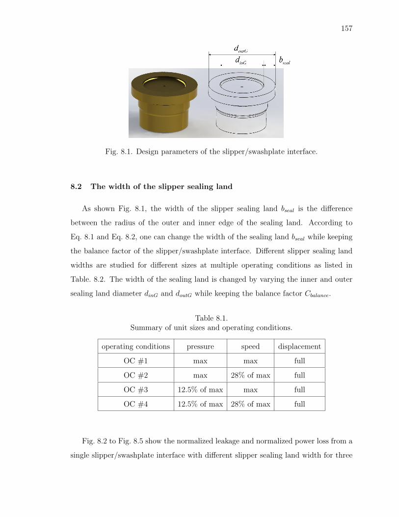
157

Fig. 8.1. Design parameters of the slipper/swashplate interface.

8.2 The width of the slipper sealing land

As shown Fig. 8.1, the width of the slipper sealing land bseal is the difference

between the radius of the outer and inner edge of the sealing land. According to

Eq. 8.1 and Eq. 8.2, one can change the width of the sealing land bseal while keeping

the balance factor of the slipper/swashplate interface. Different slipper sealing land

widths are studied for different sizes at multiple operating conditions as listed in

Table. 8.2. The width of the sealing land is changed by varying the inner and outer

sealing land diameter dinG and doutG while keeping the balance factor Cbalance.



OC #1 max max full




Fig. 8.2 to Fig. 8.5 show the normalized leakage and normalized power loss from a

single slipper/swashplate interface with different slipper sealing land width for three

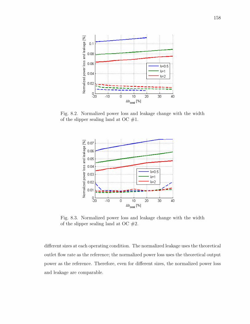
158

Fig. 8.2. Normalized power loss and leakage change with the widthof the slipper sealing land at OC #1.


different sizes at each operating condition. The normalized leakage uses the theoretical

outlet flow rate as the reference; the normalized power loss uses the theoretical output

power as the reference. Therefore, even for different sizes, the normalized power loss

and leakage are comparable.

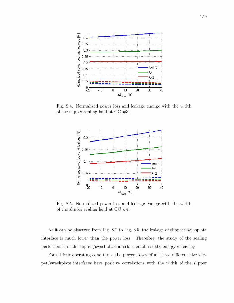
159



As it can be observed from Fig. 8.2 to Fig. 8.5, the leakage of slipper/swashplate

interface is much lower than the power loss. Therefore, the study of the scaling

performance of the slipper/swashplate interface emphasis the energy efficiency.

For all four operating conditions, the power losses of all three different size slip-

per/swashplate interfaces have positive correlations with the width of the slipper

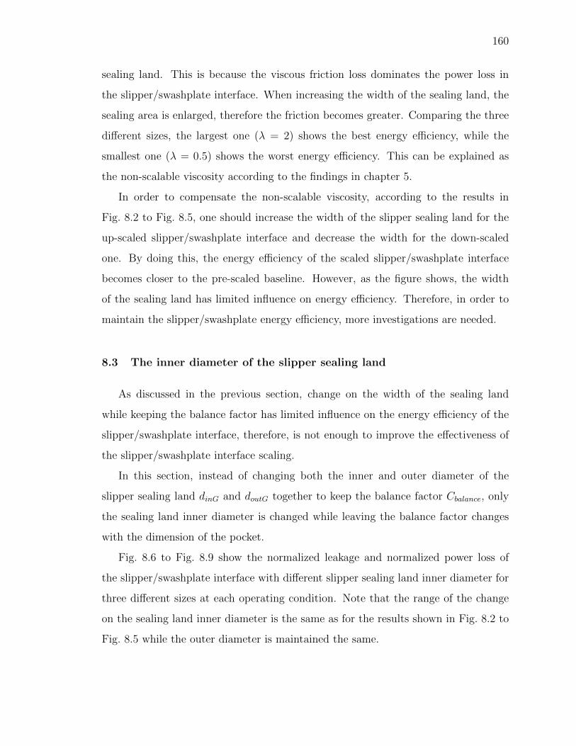
160

sealing land. This is because the viscous friction loss dominates the power loss in

the slipper/swashplate interface. When increasing the width of the sealing land, the

sealing area is enlarged, therefore the friction becomes greater. Comparing the three

different sizes, the largest one (λ = 2) shows the best energy efficiency, while the

smallest one (λ = 0.5) shows the worst energy efficiency. This can be explained as

the non-scalable viscosity according to the findings in chapter 5.

In order to compensate the non-scalable viscosity, according to the results in

Fig. 8.2 to Fig. 8.5, one should increase the width of the slipper sealing land for the

up-scaled slipper/swashplate interface and decrease the width for the down-scaled

one. By doing this, the energy efficiency of the scaled slipper/swashplate interface

becomes closer to the pre-scaled baseline. However, as the figure shows, the width

of the sealing land has limited influence on energy efficiency. Therefore, in order to

maintain the slipper/swashplate energy efficiency, more investigations are needed.

8.3 The inner diameter of the slipper sealing land

As discussed in the previous section, change on the width of the sealing land

while keeping the balance factor has limited influence on the energy efficiency of the

slipper/swashplate interface, therefore, is not enough to improve the effectiveness of

the slipper/swashplate interface scaling.

In this section, instead of changing both the inner and outer diameter of the

slipper sealing land dinG and doutG together to keep the balance factor Cbalance, only

the sealing land inner diameter is changed while leaving the balance factor changes

with the dimension of the pocket.

Fig. 8.6 to Fig. 8.9 show the normalized leakage and normalized power loss of

the slipper/swashplate interface with different slipper sealing land inner diameter for

three different sizes at each operating condition. Note that the range of the change

on the sealing land inner diameter is the same as for the results shown in Fig. 8.2 to

Fig. 8.5 while the outer diameter is maintained the same.

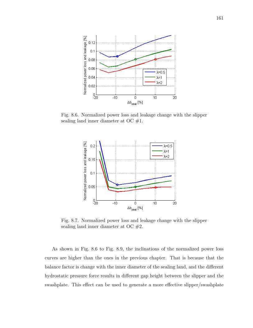
161

Fig. 8.6. Normalized power loss and leakage change with the slippersealing land inner diameter at OC #1.


As shown in Fig. 8.6 to Fig. 8.9, the inclinations of the normalized power loss

curves are higher than the ones in the previous chapter. That is because that the

balance factor is change with the inner diameter of the sealing land, and the different

hydrostatic pressure force results in different gap height between the slipper and the

swashplate. This effect can be used to generate a more effective slipper/swashplate

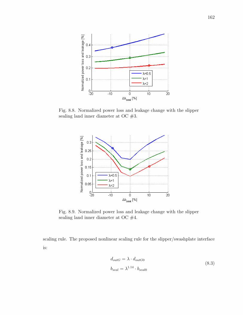
162



scaling rule. The proposed nonlinear scaling rule for the slipper/swashplate interface

is:

doutG = λ · doutG0

bseal = λ1.14 · bseal0(8.3)

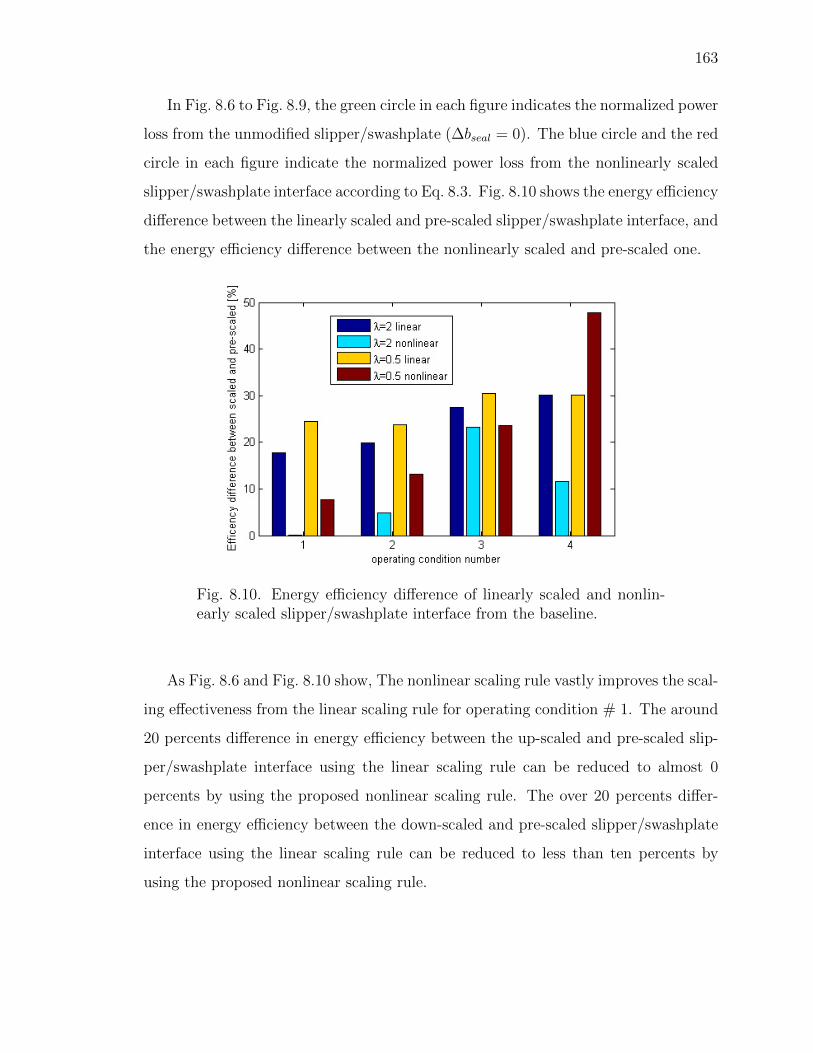
163

In Fig. 8.6 to Fig. 8.9, the green circle in each figure indicates the normalized power

loss from the unmodified slipper/swashplate (∆bseal = 0). The blue circle and the red

circle in each figure indicate the normalized power loss from the nonlinearly scaled

slipper/swashplate interface according to Eq. 8.3. Fig. 8.10 shows the energy efficiency

difference between the linearly scaled and pre-scaled slipper/swashplate interface, and

the energy efficiency difference between the nonlinearly scaled and pre-scaled one.

Fig. 8.10. Energy efficiency difference of linearly scaled and nonlin-early scaled slipper/swashplate interface from the baseline.

As Fig. 8.6 and Fig. 8.10 show, The nonlinear scaling rule vastly improves the scal-

ing effectiveness from the linear scaling rule for operating condition # 1. The around

20 percents difference in energy efficiency between the up-scaled and pre-scaled slip-

per/swashplate interface using the linear scaling rule can be reduced to almost 0

percents by using the proposed nonlinear scaling rule. The over 20 percents differ-

ence in energy efficiency between the down-scaled and pre-scaled slipper/swashplate

interface using the linear scaling rule can be reduced to less than ten percents by

using the proposed nonlinear scaling rule.

164

The similar improvement can be found for operating condition #2, as shown in

Fig. 8.7 and Fig. 8.10. The nonlinear scaling rule can reduce the scaled/pre-scaled

efficiency difference from over 20 percents to 5 percents for up-scaling and 12 percents

for down-scaling.

For operating condition #3, as shown in Fig. 8.8 and Fig. 8.10, the nonlinear

scaling rule is able to improve the scaling effectiveness but not as significant as the

previous two operating conditions. This is because, as shown in Fig. 8.8, the change

on the inner diameter of the slipper sealing land has limited influence on the slip-

per/swashplate interface efficiency at operating condition #3.

The nonlinear scaling rule improves the scaling effectiveness for up-scaling at op-

erating condition #4, however, worsen the scaling effectiveness for down-scaling. As

Fig. 8.9 show, unlike the OC #1 and OC #3, the energy dissipation increase when

reducing the width of the sealing land and increase the balance factor. The posi-

tive correlation between the energy dissipation and the balance factor indicates that

the slipper is overbalanced and lift away from the swashplate. The greatly increase

leakage start to determine the energy dissipation of the slipper/swashplate interface.

8.4 Conclusion

In this chapter, the scaling characteristic of the slipper/swashplate interface is

investigated. Three different sizes of slipper/swashplate interface are studied at four

different operating conditions as shown in Table. 8.2.

The width of the slipper sealing land bseal is first studied while the balance factor

Cbalance reminds the same. The simulation results show that the width of the sealing

land has limited impact on the performance of the slipper/swashplate, therefore, is

not enough for an effective slipper/swashplate interface scaling rule. The reason is

that the slipper/swashplate interface performance is determined by the friction loss,

which controlled by the gap height. The change on the width of the sealing land

affects the sealing function of the slipper, but not the friction loss.

165

In order to compensate the non-scalable viscosity, as found in chapter 5, the gap

height of the slipper/swashplate interface has to be controlled according to the size.

For this reason, the balance factor must not be kept the same. The second study varies

the inner diameter of slipper sealing land only, leave the balance factor changing with

the size of the slipper pocket. The simulation results show that a more effective

scaling rule for the slipper/swashplate interface can be found by nonlinearly scale the

inner diameter of the slipper sealing land as described in Eq. 8.3.

The proposed nonlinear scaling rule for the slipper/swashplate interface is able

to improve the scaling effectiveness significantly according to the simulation study as

shown in Fig. 8.10.

166

9. CONCLUSION AND OUTLOOK

For the first time, a path toward an effective scaling approach for swashplate type

axial piston machines is proposed. In this work, the scaling characteristics of the

three lubricating interfaces of swashplate type axial piston machines are investigated

and explained through the fundamental physics including the non-isothermal elasto-

hydrodynamic effects in the fluid domain and heat transfer and thermal elastic de-

flection in the solid domain. Base on the obtained knowledge, a guide for effectively

scale the critical lubricating interfaces is explored using a multi-domain multi-physics

axial piston machine performance prediction model proposed in this work.

The major contributions along the path toward an effective scaling approach for

axial piston machine can be summarized as:

• Pump and motor modeling.

• Approach for scaling analysis.

• Scaling Guidelines.

Pump and motor modeling A multi-physics multi-domain swashplate type axial

piston machine performance prediction model as shown in Fig. 4.8 is proposed

in this work. Thanks to its thermal boundaries prediction model described in

Chapter 4, this multi-physics multi-domain model can be used to study the

performance of the scaled lubricating interface without the steady-state mea-

surements. The proposed thermal boundaries prediction model calculates the

flow temperature in the outlet port volume and case volume based on the inlet

flow temperature and the temperature variation due to compression, expan-

sion, heat transfer and heat generation in the fluid domain and solid domain.

The accuracy of this temperature prediction model is validated comparing to

167

over three hundred measured outlet and case temperature for two different fluid

types, four different units, at many different speeds, operating pressures, and

swashplate angles. The proposed multi-physics multi-domain model includes

also a next-generation piston/cylinder lubricating interface model with vastly

improved accuracy and robustness as described in Chapter 3. The pressure

distribution in the fluid domain and the temperature distribution in the fluid

domain and the solid domain are calculated considering more completed physics

such as the squeezing effect of the elastic deformation and the compressibility

of the fluid. The physics are implemented in the model using more robust and

accurate numerical schemes. A elasto-hydrodynammic (EHD) pump was used

to measure the temperature distribution of the cylinder bore running surface by

using temperature sensors at 1620 different locations on the lubricating inter-

face. The simulation-measurement comparison demonstrated that the proposed

piston/cylinder interface model is able to predict the fluid film behavior with

much high accuracy as shown in Fig. 3.26 to Fig. 3.35.

Approach for scaling analysis In order to analyze the problem of the axial piston

machine scaling, an analytical study of the size-dependence of thermoelasto-

hydrodynamic tribological interfaces is conducted in this work. The physical

phenomena that were studied include the hydrostatic and hydrodynamic pres-

sure distributions, the heat transfer and the heat generation in the fluid film,

the heat transfer in the solid domain, and the solid body deformation due to

both the pressure loading and the thermal load. The analysis indicates that

the pressure distribution in the lubricating gap and the heat transfer in the

fluid and in the solid bodies are the only size-dependent physical phenomena;

therefore, they are the only contributors to the performance change of the lu-

bricating interface in response to scaling. These findings allow for the creation

of a general guide to scale aiming at maintaining the efficiency of the original

unit. The guide suggests that different fluid, different working conditions, and

different designs can be used to compensates the non-scalable pressure distri-

168

bution and heat transfer. The scaling guide enables pump manufacturers to

apply the developed scaling laws, and efficiently generate scaled pump designs

of much higher efficiency than the traditional approach of linear scaling allows

for.

Scaling Guidelines With the proposed scaling guide, all three lubricating interfaces

of swashplate type axial piston machine are studied for different sizes (9.375 cc,

75 cc, and 600 cc) at multiple operating conditions, and a more effective scaling

rule is proposed for each interface:

• Nonlinearly scaled piston/cylinder clearance with proposed groove profile

allows to maintain the volumetric efficiency of the scaled interface very

close to the original size, and to keep energy efficiency of the up-scaled

interface above the value for the original size.

• Nonlinearly scaled cylinder block/valve plate interface sealing land and

kidney shape opening show much better effectiveness than the linear scal-

ing law.

• Nonlinearly scaled slipper balance factor, which defined as the ratio be-

tween the hydrostatic pressure force and the external load, by nonlinearly

scale the inner diameter of the sealing land, is able to compensate the

non-scalable viscous friction and achieve more effective slipper/swashplate

interface scaling.

This work describes a path toward the effective scaling approach for the swashplate

type axial piston machine. With continued effort, the scaling process can be less

monetary and temporal expensive. A highly efficient unit design can be used as a

baseline to create a series of high quality pumps and motors across a wide range of

unit size with minimum effort.

Beyond the scope of this work, future works on this topic include improving the

fidelity of the lubricating interface fluid film behavior simulation tool by using a

169

finer fluid grid with possibly adaptive grid refining algorithm to further improve the

accuracy of the model. The more advanced tribological effect can be considered

in the lubricating interfaces model in the future, such as mixed friction and the

slip boundary. More advanced technologies can be implemented in the simulation

to accelerate the converging process, such as multi-core, multi-thread, and general

purpose graphic processing unit (GPU) computing.

Other future works can be done on the scaling study includes more productive case

study practice. A more effective scaling rule can be found using advanced optimization

algorithm and the artificial intelligent technology such as neural network and machine

learning.

Since as mentioned in Chapter 5, the findings of the analysis of the size-dependence

of the lubricating interfaces is not limited to swashplate type axial piston machines,

the scaling study for other types of lubricating interfaces in axial piston machines,

radial piston machines, internal and external gear pumps and motors, gerotors, vane

pumps, bearings and seals can be conducted based on this work.

Back to the swashplate type axial piston machine, the tolerance and surface rough-

ness should also be considered in the future scaling study. The performance of the

swashplate type axial piston machine other than the energy efficiency should also be

investigated in the future such as noise and vibration.

REFERENCES

170

REFERENCES

[1] J. Ivantysyn and M. Ivantysynova, Hydrostatic pumps and motors: principles,design, performance, modelling, analysis, control and testing. Tech Books In-ternational, 2003.

[2] N. D. Manring, C. L. Wray, and Z. Dong, “Experimental studies on the perfor-mance of slipper bearings within axial-piston pumps,” Journal of tribology, vol.126, no. 3, pp. 511–518, 2004.

[3] N. D. Manring, “Tipping the cylinder block of an axial-piston swash-plate typehydrostatic machine,” Journal of dynamic systems, measurement, and control,vol. 122, no. 1, pp. 216–221, 2000.

[4] ——, “Friction forces within the cylinder bores of swash-plate type axial-pistonpumps and motors,” Journal of dynamic systems, measurement, and control, vol.121, no. 3, pp. 531–537, 1999.

[5] J. S. Sartchenko, “Force balance condition of the valve plate and rotor of an axialpiston pump,” British Hydromechanics Research Association, Tech. Rep. T750,1950.

[6] N. Franco, “Pump design by force balance,” Hydraulics & Pneumatics, vol. 14,no. 11, pp. 101–107, 1961.

[7] A. Yamaguchi, “Formation of a fluid film between a valve plate and a cylinderblock of piston pumps and motors: 2nd report, a valve plate with hydrostaticpads: heat transfer, combustion, power, thermophysical properties,” JSME in-ternational journal, vol. 30, no. 259, pp. 87–92, 1987.

[8] ——, “Formation of a fluid film between a valve plate and a cylinder block ofpiston pumps and motors: 1st report, a valve plate with hydrodynamic pads,”Bulletin of JSME, vol. 29, no. 251, pp. 1494–1498, 1986.

[9] A. Yamaguchi, H. Sekine, S. Shimizu, and S. Ishida, “Bearing/seal characteristicsof the film between a valve plate and a cylinder block of axial piston pumps. Ef-fects of fluid types and theoretical discussion,” Journal of Fluid Control, vol. 20,no. 4, pp. 7–29, May 1990.

[10] H. Merritt, Hydraulic control systems. John Wiley & Sons, 1967.

[11] N. D. Manring, R. E. Johnson, and H. P. Cherukuri, “The impact of lineardeformations on stationary hydrostatic thrust bearings,” Journal of Tribology,vol. 124, no. 4, pp. 874–877, 2002.

[12] N. D. Manring, “Valve-plate design for an axial piston pump operating at lowdisplacements,” Journal of mechanical design, vol. 125, no. 1, pp. 200–205, 2003.

171

[13] O. Reynolds, “Iv. on the Theory of Lubrication and Its Application to Mr.Beauchamp Towers Experiments, Including an Experimental Determination ofthe Viscosity of Olive Oil,” Philosophical Transactions of the Royal Society ofLondon, vol. 177, pp. 157–234, 1886.

[14] M. Pelosi, “An investigation of the fluid-structure interaction of piston/cylinderinterface,” Ph.D. dissertation, Purdue University, 2012.

[15] H.-J. van der Kolk, “Beitrag zur Bestimmung der Tragfhigkeit des stark verkan-teten Gleitlagers Kolben/Zylinder an Axialkolbenpumpen der Schrgscheiben-bauart,” Ph.D. dissertation, Verlag nicht ermittelbar, 1972.

[16] A. Yamaguchi and Y. Tanioka, “Motion of pistons in piston-type hydraulic ma-chines: 1st. report: theoretical analysis,” Bulletin of JSME, vol. 19, no. 130, pp.402–407, 1976.

[17] M. Ivantysynova, “An investigation of viscous flow in lubricating gaps,” Ph.D.dissertation, SVST Bratislava, Czechoslovakia, 1983.

[18] Y. Fang and M. Shirakashi, “Mixed lubrication characteristics between the pistonand cylinder in hydraulic piston pump-motor,” Journal of tribology, vol. 117,no. 1, pp. 80–85, 1995.

[19] L. Olems, “Investigations of the temperature behaviour of the piston cylinderassembly in axial piston pumps,” International Journal of Fluid Power, vol. 1,no. 1, pp. 27–39, 2000.

[20] M. Ivantysynova and C. Huang, “Investigation of the gap flow in displacementmachines considering elastohydrodynamic effect,” in Proceedings of the JFPSInternational Symposium on Fluid Power, vol. 2002. The Japan Fluid PowerSystem Society, 2002, pp. 219–229.

[21] M. Pelosi and M. Ivantysynova, “A novel thermal model for the piston/cylinderinterface of piston machines,” in ASME 2009 Dynamic Systems and ControlConference. American Society of Mechanical Engineers, 2009, pp. 37–44.

[22] ——, “Heat transfer and thermal elastic deformation analysis on the pis-ton/cylinder interface of axial piston machines,” Journal of tribology, vol. 134,no. 4, p. 041101, 2012.

[23] M. Zecchi, “A novel fluid structure interaction and thermal model to predict thecylinder block/valve plate interface performance in swash plate type axial pistonmachines,” Ph.D. dissertation, Purdue University, 2013.

[24] U. Wieczorek and M. Ivantysynova, “Computer aided optimization of bearingand sealing gaps in hydrostatic machinesthe simulation tool CASPAR,” Inter-national Journal of Fluid Power, vol. 3, no. 1, pp. 7–20, 2002.

[25] C. Huang, “A new approach to predict the load carrying ability of the gap be-tween valve plate and cylinder block,” in Bath Workshop of Power Transmissionand Motion Control PTMC 2003, Bath, UK, 2003, pp. 225–239.

[26] M. Zecchi and M. Ivantysynova, “A novel fluid structure interaction model forthe cylinder block/valve plate interface of axial piston machines,” Proceedings ofthe IFPE, 2011.

172

[27] ——, “A novel approach to predict the cylinder block/valve plate interface per-formance in swash plate type axial piston machines,” in ASME/Bath Symposiumon Fluid Power and Motion Control, 2012, pp. 13–28.

[28] A. T. Schenk, “Predicting lubrication performance between the slipper andswashplate in axial piston hydraulic machines,” Ph.D. dissertation, Purdue Uni-versity, 2014.

[29] N. A. Shute and D. E. Turnbull, “The losses of hydrostatic slipper bearings un-der various operating conditions,” British Hydromechanics Research Association,Tech. Rep. RR743, Oct. 1962.

[30] ——, “The minimum power loss of hydrostatic slipper berrings,” BHRA, Tech.Rep. SP721, 1962.

[31] C. J. Hooke and K. Y. Li, “The lubrication of overclamped slippers in axial pistonpumpscentrally loaded behaviour,” Proceedings of the institution of mechanicalengineers, part c: journal of mechanical engineering science, vol. 202, no. 4, pp.287–293, 1988.

[32] ——, “The lubrication of slippers in axial piston pumps and motorsthe effect oftilting couples,” Proceedings of the institution of mechanical engineers, part c:journal of mechanical engineering science, vol. 203, no. 5, pp. 343–350, 1989.

[33] A. Schenk, M. Zecchi, and M. Ivantysynova, “Accurate prediction of axial pis-ton machines performance through a thermo-elasto-hydrodynamic simulationmodel,” in ASME/BATH 2013 Symposium on Fluid Power and Motion Con-trol. American Society of Mechanical Engineers, 2013, pp. V001T01A034–V001T01A034.

[34] A. Schenk and M. Ivantysynova, “A transient thermoelastohydrodynamic lubri-cation model for the slipper/swashplate in axial piston machines,” Journal ofTribology, vol. 137, no. 3, p. 031701, 2015.

[35] K. T. Renius, Untersuchungen zur Reibung zwischen Kolben und Zylinder beiSchrgscheiben-Axialkolbenmaschinen. VDI-Verlag, 1974.

[36] R. Lasaar, Eine Untersuchung zur mikro-und makrogeometrischen Gestaltung derKolben-, Zylinderbaugruppe von Schrgscheibenmaschinen. VDI-Verlag, 2003.

[37] R. A. Burton, “Paper 5: The Thermodynamics of a Viscoelastic Film underShear and Compression,” in Proceedings of the Institution of Mechanical Engi-neers, Conference Proceedings, vol. 180. SAGE Publications Sage UK: London,England, 1965, pp. 72–84.

[38] G. Xu and F. Sadeghi, “Thermal EHL analysis of circular contacts with measuredsurface roughness,” Journal of tribology, vol. 118, no. 3, pp. 473–482, 1996.

[39] H. Everth, “Konstruktion einer Modellpumpe zur Messung des Druck-und Tem-peraturfeldes im Spalt zwischen Kolben und Zylinder einer Schragscheiben-Axialkolbenmaschine,” Ph.D. dissertation, TUHH, 2003.

[40] L. Shang and M. Ivantysynova, “Advanced heat transfer model for pis-ton/cylinder interface,” in Proceedings of the 11th IFK International Fluid PowerConference, vol. 1, Aachen, Germany, Mar. 2018, pp. 587–595.

173

[41] ——, “Thermodynamic analysis on compressible viscous flow and numericalmodeling study on piston/cylinder interface in axial piston machine,” in Pro-ceedings of the 10th JFPS International Symposium on Fluid Power, Fukuoka,Japan, 2017, pp. 475–581.

[42] D. Grnberg, “Prediction of case temperature of axial piston pumps,” Master’sthesis, Chalmers University of Technology, Sweden, 2011.

[43] M. Zecchi, A. Mehdizadeh, and M. Ivantysynova, “A novel approach to predictthe steady state temperature in ports and case of swash plate type axial pistonmachines,” in 13th Scandinavian International Conference on Fluid Power; June3-5; 2013; Linkping; Sweden. Linkping University Electronic Press, 2013, pp.177–187.

[44] L. Shang and M. Ivantysynova, “Port and case flow temperature prediction foraxial piston machines,” International Journal of Fluid Power, vol. 16, no. 1, pp.35–51, 2015.

[45] ——, “An investigation of design parameters influencing the fluid film behav-ior in scaled cylinder block/valve plate interface,” in 9th FPNI Ph. D. Sympo-sium on Fluid Power. American Society of Mechanical Engineers, 2016, pp.V001T01A027–V001T01A027.

[46] ——, “A path toward effective piston/cylinder interface scaling approach,” inASME/BATH 2017 Symposium on Fluid Power and Motion Control. AmericanSociety of Mechanical Engineers, 2017, pp. V001T01A072–V001T01A072.

[47] ——, “A temperature adaptive piston design for swash plate type axial pistonmachines,” International Journal of Fluid Power, vol. 18, no. 1, pp. 38–48, 2017.

APPENDICES

174

VITA

Lizhi Shang was born on March 25th, 1989 in Tianjin, China. He received this B.S.

from Huazhong University of science and technology in June 2011. In fall of 2011, he

began as a master student in New Jersey Institute of technology. In Summer of 2012,

he joined Maha fluid power research center for two months as a visiting student. He

officially became a graduate student at Maha fluid power research center at Purdue

University since January 2013 under the supervision of Dr. Monika Ivantysynova.

His research focus was studying the scaling of axial piston pumps and motors. He

successfully defended his Ph.D. in November 2018.

a path toward an effective scaling approach for axial

Documents

Transcript of a path toward an effective scaling approach for axial