A parallel implementation of nec for the analysis of large structures

1

Submitted to IEEE Trans. EMC

A Parallel Implementation of NEC for the

Analysis of Large Structures

A. Rubinstein, F. Rachidi Swiss Federal Institute of

Technology Lausanne

Switzerland

M. Rubinstein School of Applied

Sciences of Western Switzerland,

Yverdon, Switzerland

B. Reusser Defense Procurement Agency

NEMP-Labor Spiez, Switzerland

Abstract - We present a new, parallel version of the Numerical Electromagnetics Code (NEC). The

parallelization is based on a bi-dimensional block-cyclic distribution of matrices on a rectangular processor grid,

assuring a theoretically-optimal load balance among the processors. The code is portable to any platform

supporting message passing parallel environments such as MPI and PVM where it could even be executed on

heterogeneous clusters of computers running on different operating systems. The developed parallel NEC was

successfully implemented on two parallel supercomputers featuring different architectures to test portability.

Large structures containing up to 24’000 segments, which exceeds currently available computer resources were

successfully executed and timing and memory results are presented. The code is applied to analyze the

penetration of electromagnetic fields inside a vehicle. The computed results are validated using other numerical

methods and experimental data obtained using a simplified model of a vehicle (consisting essentially of the body

shell) illuminated by an EMP simulator.

I. INTRODUCTION

The Numerical Electromagnetics Code (NEC) is a user-oriented computer code based on the method of

moments and written in FORTRAN for the analysis of the electromagnetic response of antennas and other metal

structures [1,2,3]. It has been widely used with great success for radio communications testing as well as antenna

design and EMC. With its ability to represent models by means of wires, the code should also allow the

simulation of very complex 3D structures [1].

2

NEC produces an interaction matrix representing the system of integral equations needed to obtain the currents

and fields. The number of elements in this matrix depends on the number of segments and patches that conform

the model to be evaluated. This matrix is then reduced using LU factorization and, together with the excitation

vector, the final solution to the integral equations is obtained [1].

For a model consisting of N segments, a good approximation to the amount of memory in bytes required by

NEC is given by this expression:

162 ⋅= NMem (1)

Notice the quadratic dependence of the growth of the memory requirements with the number of segments. The

required amount of memory becomes important on many current computers at around 2000 segments since, for

that particular case, approximately 64 MB of RAM are necessary to complete program execution. With 128 MB

of RAM, the number of segments that fit in memory won’t even reach 3000. In order to run even larger models,

virtual memory can be used but at a very high price in terms of time. The use of the hard disk, by means of a

swap file, will slow down the execution of NEC to unpredictable values (see Section III). An ‘out of core’

routine is embedded into NEC to optimize performance in these cases. The matrix is cut in pieces that are stored

on the hard disk, following a special pattern. The operating system can then use all available RAM and NEC will

take care of disk swapping. The out of core routine requires about four times the normal RAM and, as a

consequence, enormous swap files are created [1].

One might think that having as much memory as needed is the best way to assure optimal execution. However,

operating systems are not capable of managing all the memory one would be prepared to buy. A version of NEC

compiled for a very large number of segments will fail to start because operating systems are unable to allocate it

in memory.

In this paper, we present a parallel version of the Numerical Electromagnetics Code (NEC). Excell et al. [4]

presented a modified version of NEC to optimize performance on a four-processor Cray X-MP computer. This is

a shared memory machine with a low degree of parallelism. Nitch and Fourié [5, 6] re-implemented NEC using

C++ and produced a modified version capable of running in parallel. The parallel version of NEC we present

works on distributed memory parallel supercomputers and is portable to any platform supporting typical message

passing parallel environments such as MPI (Message Passing Interface) and PVM (Parallel Virtual Machine). It

is entirely based on the original NEC core written in FORTRAN, and it does not require any modifications to be

made to classic NEC input files. The output files have also an identical format to those produced by the original

NEC, so any existing NEC post-processing tool may be used. Some small models have been tested in both, the

3

original NEC and the proposed parallel version and we have found the numerical results to be identical. The

proposed parallel version of NEC is available for free to the academic community and the source is open, so that

the code may be changed, adapted or improved.

The parallel implementation is thoroughly described in Sect. II. The code is implemented on two

supercomputers belonging to the Swiss Federal Institute of Technology, and its performance in terms of memory

and solution time is presented in Section III. Section IV contains an application of the developed code to the

analysis of the penetration of electromagnetic fields inside a vehicle. The computed results were validated using

(1) other numerical methods and (2) experimental data obtained using the VERIFY EMP simulator belonging to

the Swiss Defense Procurement Agency. The VERIFY simulator generates a vertically-polarized electric field

with a rise time of 0.9 ns and a FWHM of 24 ns. Measurements of electromagnetic fields inside a simplified

model of a car (consisting essentially of the body shell) were performed considering two types of illumination,

front and side. The results of the validation are also included in Section IV. A short summary and conclusions

are given in Section V.

II. PARALLEL IMPLEMENTATION OF NEC

Computer resources at the time NEC was written were very different from those available today. With almost

10’000 lines, this code has been conceived for linear operation.

Figure 1 shows a modified version of the original flow diagram of the main section of NEC reflecting the

changes imposed by the parallelization process. NEC is globally composed of two parts: (1) the input section (on

the left hand side of Figure 1), which reads in geometrical information about the model and stores the cards that

dictate additional model information, program commands and directives of execution; and (2) the calculation

section (on the right hand side of the figure), which computes the coefficients to produce [G] for the matrix

equation [G] [I]=[E] where [G] is the so-called interaction matrix, holding geometrical and electromagnetic

information about the structure, [I] is a vector holding the current on each element and [E] represents the

excitation vector. This section of the code also solves this equation by means of the Gauss-Doolittle matrix-

triangulation method. The method has been divided into two routines; the first carries out an LU decomposition

of the interaction matrix [G] [1], which is then passed to a second routine together with the excitation vector [E]

to determine the solution of the system. The better part of the computational effort goes into factoring [G] into

[L] and [U]. In fact, computation of the elements of the interaction matrix [G] and the solution of the matrix

equation are the two most time-consuming steps in calculating the response of a structure, often accounting for

4

over 90% of the computation time [1]. For that reason, we decided to concentrate the parallelization effort on

that part of the code.

A parallel implementation of the LU decomposition and the parallel solution of the system of equations require

the distribution of the information stored in the matrices among the available processors. This means that

matrices [G] and [E] need to be cut into smaller sub-matrices that will be local to each processor. In order to

evenly distribute the calculation effort among all available processors, this distribution must follow a special

pattern known as the two-dimensional block-cyclic distribution or decomposition [7].

5

Start of new case Read and print comments

Call DATAGN to read structure data

Read data card

STOP

Branch to section for particular card

Calculation Request?

EN Card?

NX Card?

Go to B

A

yes

yes

yes

No

No

No

B

Element (i,j) belongs to

local matrix?

Compute interaction matrix element (i,j)

Compute local (i,j) according to block cyclic

distribution pattern

No

yes

Parallel LU Decomposition with all

available processors

Set excitation array

Distribute excitation array block cyclically

Parallel solve for current with all available

processors Collect local results

Compute input power, efficiency, etc.

Compute near field, radiated field if requested

Go to A

Startup parallel environment

Matrix Generation Routine

Calculation Section

Input Section

Fig. 1 – Flow diagram of the developed Parallel NEC. Shaded: modified or newly created parallel code.

Consider a parallel computer with 4 processors labelled from 0 to 3 and a matrix to be distributed. At first, one

would be tempted to think that the most logical way to distribute the information among the 4 processors would

follow the layout shown in Figure 2a. Figure 2b shows the result of applying the two-dimensional block cyclic

6

distribution with the same number of processors to the same matrix. Processor 0 holds the shaded parts of the

matrix. As it can be seen, the block cyclic decomposition is a “far from intuitive” form of distribution for the

matrices.

(a) One-dimensional column distribution (b) Two-dimensional block cyclic distribution

Fig. 2 – Distribution of matrix among 4 processors.

The implementation of the Gaussian Elimination algorithm, a key component of the Gauss-Doolittle numerical

method, iterates on the matrix by rows and columns, from left to right, and from top to bottom. If we use the

one-dimensional column distribution (Fig. 2a), after a certain number of iterations, all the elements in the

leftmost group, labelled 0, would have been calculated, thus, leaving processor 0 idle during a significant part of

the calculation time. Once all the elements that correspond to processor 1 have been calculated, this processor,

too, will become idle, for the remainder of the calculation time. The same type or reasoning may be applied in

turn to the other two processors. On the other hand, the use of the two-dimensional block cyclic decomposition

in Figure 2b assures that, on average, all of the processors contribute to the final solution from the beginning to

the end of the algorithm. Better performance may be obtained if the processor grid is square since, this way, it is

easier to do a more equitable distribution of the calculation load. Since the number of processors may vary from

one machine to another, a square processor grid remains a desirable condition rather than a requisite and, in

practice, the grid is made as square as possible. This is achieved by way of an automatic calculation of the

squarest possible processor grid on the running platform performed at the beginning of the developed parallel

NEC and used to declare and start the parallel environment. The block cyclic decomposition used in the

developed parallel NEC is based on the SCALAPACK library [8], a very powerful, parallel implementation of a

subset of routines contained in the Linear Algebra Package (LAPACK).

0 1 0 1 0 1 0 1 2 3 2 3 2 3 2 3 0 1 0 1 0 1 0 1 2 3 2 3 2 3 2 3 0 1 0 1 0 1 0 1 2 3 2 3 2 3 2 3 0 1 0 1 0 1 0 1

3 2 3 2 3 3 2 2

1

0

2

3

7

Clearly the construction of the interaction matrix on a single computer to be distributed later among the

computers in the grid, would not solve the memory problem. A new implementation of the matrix filling routine

had to be written in order to produce an already distributed matrix as it is being calculated. After execution of the

input section in Figure 1, every processor on the grid holds the information needed to calculate the elements of

[G]. One newly created function indicates to each processor of the cluster if the element (i, j) being calculated

corresponds to its local sub-matrix. If this is the case, a subroutine will calculate the local values of (i, j) for the

same element so that it can be assigned to the corresponding local matrix. At the end of the modified matrix

generation routine indicated in Figure 1, each processor will hold its local version of the interaction matrix

without the need for explicit communication operations among the processors. The dimensions of the interaction

matrix array are assigned at runtime based on the calculated dimensions of the local sub-matrices, which depend

on the number of processors in use. The code adapts automatically to the environment and to the number of

processors. The dimensions of the rest of the arrays need to be indicated at compilation time1.

The LU decomposition in NEC is carried out in the matrix factorization routine (called FACTR). After this

routine is executed, the interaction matrix [G] can be expressed as:

[ ] [ ][ ]ULG = (2)

and the matrix equation becomes:

[ ][ ][ ] [ ]EIUL = (3)

The solution is then computed in the solving routine (called SOLVE), solving for F by forward substitution in

[ ] [ ][ ]EFL = (4)

and solving for I by backward substitution in

[ ] [ ][ ]FIU = (5)

Both the FACTR and SOLVE routines have been rewritten to produce parallel equivalents. 1 NEC reads all the geometrical and electromagnetic information from the input file before calculating the interaction matrix. This information is stored in arrays which, in the proposed parallel version of NEC, remain identical to the original version. Since these arrays are passed to subroutines using common blocks, their dimensions need to be explicitly declared at compilation time.

8

Vector [E] needs to be block-cyclically distributed as well. This task is carried out by a routine that

automatically assigns values and indices. After the solution [I] is found, data are put back together by means of a

block-cyclic composition routine and all of the processors become aware of the solution. Normal program

execution can continue and solutions can be printed to the output file.

As a consequence of the matrix distribution among the processors, in the parallel version of NEC, the memory

requirements for each one of the local sub-matrices are inversely proportional to the number of processors. For

example, a model consisting of 11500 segments requires approximately 2 GB of RAM running on only 1

processor. If 16 processors with 128 MB of RAM each are used to solve the same problem, the memory gets

shared and the model might be successfully executed without swapping matrix information between memory and

disk. As a general rule, an estimate of the memory requirements in bytes at a local node for the parallel version

of NEC can be calculated using this expression:

P

NMem 162 ⋅= (6)

where P is the number of processors being used at runtime.

III. TEST AND PERFORMANCE Our testing was carried out using one PC with a PIII processor running at 750 MHz with Windows NT 4.0 and

256 MB of RAM and 2 distributed memory machines, the Swiss-T1 [9] and Eridan [10]. The Swiss-T1, one of

the fastest supercomputers in Switzerland, features 35 Compaq DS20E dual Alpha processor boxes at 500 MHz

each. They all have 1 GB of RAM and two 9.1 GB SCSI-U2 hard disks. Two of those boxes are used as an

interactive front-end, another one for upgrades, development and maintenance, and the other 32 are used as

calculation nodes. This 64-processor calculation part is connected by a Tnet network, which is a reliable, high

performance, low latency network to build commodity-supercomputing clusters. The Eridan supercomputer has

128 MIPS R14000 RISC super-scalar CPU’s running at 500 MHz each and distributed among 32 nodes. Each

processor has 512 Mbytes of RAM for a total of 64 Gbytes. The total capacity of the hard disks goes up to 1.5

TB for system and users.

The first NEC input file used for testing, a rectangular wiregrid representation of a car, consisted of 6753

segments. Figure 3 shows a 3D plot of this simple model. In this case, the Eridan computer was only used to test

portability of the code. On the Swiss-T1, the same input file was executed with 4, 8, 16, 24, 32 and 36

processors. We have found the numerical results from both computers to be the same within working precision.

9

For Eridan, no timing or memory results are presented here. Table 1 shows the relation of the number of

processors on the Swiss-T1 with matrix filling, matrix factorization and run times, local memory and total

memory.

On the PC, we specified that the maximum core storage should be limited to 2000 segments since the total

model requires about 700 MB. This would leave enough space for the operating system and services and should

allow flawless calculation using the out of core routine included in NEC.

Fig. 3 – NEC mesh of the simplified car consisting of 6753segments used for performance comparisons.

Examining Table 1, it can be seen that the use of only 4 processors reduces run time to a small fraction of the

original, only 1.9%. This is mainly due to the fact that the PC is forced to use disk swapping. Per processor

memory behaves as expected. It is important to notice that the memory used by each single processor depends on

the particular dimensions of its local matrix, and that the values given in the table are the largest. The total

memory for each parallel configuration is higher than the PC's theoretical requirements because the rest of the

arrays that are used in the parallel version need to be declared with the total size of the model.

Table 1 – Timing and memory as a function of the number of processors for a 6753 segments test case.

Number of Processors

Matrix Filling Time

Matrix Facto-rization time

Run Time (2 freq. Steps)

Mem/processor (MB)

Total Memory (MB)

1 – PC 10 min 6 h 47 min 14 h 6 min 62* 2790

4 – T1 2 min 56 sec 5 min 24 sec 16 min 7 sec 193.9 769.34





36 – T1 3 min 1 min 3 sec 8 min 34 sec 28.45 988.57

*Approximation based on a core storage of 2000 segments.

10

In figures 4 and 5, we present the matrix factorization time and the total run time as a function of the number

of processors. From these figures, we observe that the use of too large a number of processors can compromise

the total run time. We noticed that, for our particular experiment, the matrix filling time did not respond linearly

to the number of processors as the factorization and solution routines did. This may be due to the fact that the

matrix filling does not use any parallel-optimized functions or routines but depends on the particular

configuration of the parallel cluster and the number of elements in the matrix, making it hard to predict the

execution time as a function of the number of processors. The appropriate selection of the number of processors

related to the dimensions of the model is the subject of further study.

Matrix Factorization Time6753 segments

050

100150200250300350

0 10 20 30 40


Tim

e (s

)

Fig. 4 – Matrix factorization time as a function of number of processors.

Parallel NEC Run Time6753 segments

0200400600800

10001200

0 10 20 30 40


Tim

e (s

)

Fig. 5 – Total run time as a function of number of processors.

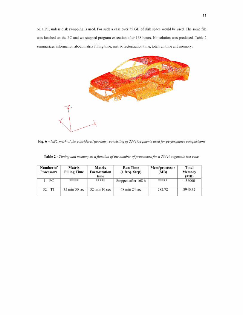
A larger structure consisting of 23449 segments, a more complex representation of a car using a triangular grid

was also tested (see figure 6). With this number of segments, approximately 8.4 GB of RAM are required. The

total execution time on the Swiss-T1 with 32 processors was about 68 minutes. This example cannot be executed

11

on a PC, unless disk swapping is used. For such a case over 35 GB of disk space would be used. The same file

was lunched on the PC and we stopped program execution after 168 hours. No solution was produced. Table 2

summarizes information about matrix filling time, matrix factorization time, total run time and memory.

Fig. 6 – NEC mesh of the considered geoemtry consisting of 23449segments used for performance comparisons

Table 2 - Timing and memory as a function of the number of processors for a 23449 segments test case.


Matrix Filling Time

Matrix Factorization

time

Run Time (1 freq. Step)

Mem/processor (MB)

Total Memory

(MB) 1 – PC ***** ***** Stopped after 168 h ***** ~36000


12

IV. VALIDATION OF THE PARALLEL NEC: STUDY OF THE FIELD PENETRATION INSIDE A

VEHICLE ILLUMINATED BY AN EMP SIMULATOR

A. Description of the Configuration and Experimental Results

The automobile industry has been increasing the amount of on-board technology. Modern cars exhibit

navigation systems, high-tech entertainment devices, and computer-controlled optimization of fuel injection,

brakes, etc. As a consequence, the study of the EMC phenomena in automobiles becomes indispensable (e.g.

[11,12]). In order to test the developed parallel NEC code, we have used experimental data obtained in the

framework of the European GEMCAR (Guidelines for Electromagnetic Compatibility Modelling for

Automotive Requirements) project.

The experiments were carried out using VERIFY (Vertical EMP Radiating Indoor FacilitY), an EMP simulator

belonging to the Swiss Defense Procurement Agency (Spiez) (Fig. 7). VERIFY generates a vertically polarized

electric field with a rise time of 0.9 ns and a FWHM of 24 ns. The working volume is 4x4x2.5 m3 and the

maximum E-field amplitude is 100 kV/m. A cartography of the E-field produced by the simulator was created by

taking several measurements at 1 m above the ground and at square intervals of 1 m. This grid was used for

checking the homogeneity of the produced field. Figure 8 shows the incident electric field measured inside the

working volume of the VERIFY in the absence of any structure.

Fig. 7 – VERIFY EMP Simulator.

For the electric and magnetic field measurements we used Thomson MELOPEE-E1602 and H1602 sensors,

designed for measuring free space electric and magnetic fields, sinusoidal or pulsed, up to 1.2 GHz.

13

The data acquisition system featured a fiber optics link between the sensors and a digitizer with a sampling rate

of 2 GSamples/s.

A simple test case was defined using a Volvo S80 body shell without doors or glazing. The car was placed

inside the working volume of the simulator (Fig. 9) and four points, P3, P4, P5 and P6 (see Figure 10) were

selected in the passengers’ compartment for E and H measurements.

-10

0

10

20

30

40

50

60

0 200 400 600 800 1000

Inci

dent

Ele

ctric

Fie

ld E

z (k

V/m

)

Time (ns)

Fig. 8 – Vertical electric inside the working volume of the simulator.

Fig. 9 – Test car inside the simulator.

14

Fig. 10 – Illustration of the two measurements points inside the vehicle.

Figure 11 presents the waveforms of the vertical component of the electric field measured at points P3 to P6

for front and side illuminations. A thorough analysis of the experimental data may be found in [13].

-10

0

10

20

30

40

0 0.2 0.4 0.6 0.8 1

P3 - Electric Field z-Component - Front

Ez (k

V/m

)

time (µs)

-10

-5

0

5

10

15

20

25

0 0.2 0.4 0.6 0.8 1

P3 - Electric Field z-Component - Side

Ez (k

V/m

)

time (µs)

15

-15

-10

-5

0

5

10

15

20

0 0.2 0.4 0.6 0.8 1


Ez (k

V/m

)

time (µs)

-10

-5

0

5

10

15

20

0 0.2 0.4 0.6 0.8 1


Ez (k

V/m

)

time (µs)

-20

0

20

40

60

80

0 0.2 0.4 0.6 0.8 1


Ez (k

V/m

)

time (µs)

-10

0

10

20

30

40

0 0.2 0.4 0.6 0.8 1


Ez (k

V/m

)

time (µs)

-15

-10

-5

0

5

10

0 0.2 0.4 0.6 0.8 1


Ez (k

V/m

)

time (µs)

-20

-15

-10

-5

0

5

10

15

0 0.2 0.4 0.6 0.8 1


Ez (k

V/m

)

time (µs)

Fig. 11 – Vertical electric field component measured at Points P3, P4, P5 and P6. Left column: front

illumination, right column: side illumination.

16

B. Comparison with Other Numerical Methods

As a first step in validating the code, numerical results obtained using the parallel NEC have been compared to

those obtained using other, well known numerical techniques (TLM [14,15]), hybrid FV/FDTD [16] and BEM

[17]). The point used for comparison was P4, located at the centre of the vehicle. The geometrical information

about the model was obtained from the same original CAD data and it was adapted to fit particular requirements

of each individual method. Figure 12 shows the adapted meshing of the model for each numerical method

applied and Figure 13 shows a comparison of the simulation results. An excellent agreement was found.

(a) – Mesh FDTD of the car

(b) – Mesh BEM of the car

(c) – Mesh TLM of the car

(d) – Mesh NEC of the car

Fig. 12 – Meshing of the different numerical methods used for validation (Adapted from [18])

17

0

5 10-5

0.0001

0.00015

0.0002

0.00025

0.0003

107 108 109

BEMParallel NECFDTD HybridTLM

Verti

cal E

lect

rif F

ield

(V/m

/Hz)

Frequency (Hz)

Fig. 13 – Comparison of the numerical results from different methods.

C. Comparison with Experimental Data

The geometrical data for the simulated car were obtained from a CAD file. This file was manipulated to

represent the stripped-down version of the test car (i.e. only the body shell). We have already shown the 3D

representation of the NEC input file in Figure 12. This model was converted and adapted from the TLM version

of the CAD data. The excitation was provided by a simulated unitary vertically polarized plane wave produced

by NEC. Since NEC is a frequency domain tool, the measured data were converted to the frequency domain

using the FFT and incident field measurements performed in the absence of any object inside the simulator were

used to properly adapt the simulations to the excitation. The NEC model consisting of almost 8000 segments was

run on 16 processors. Average run time for one frequency step was 7 minutes.

Figures 14 and 15 show comparisons of measurements and simulations for the vertical component of the

electric field at the four observation points defined inside the car for both, front and side illumination. The fields

are normalized with respect to the incident field located at the centre of the EMP simulator. We can see that the

simulations are in very good agreement with the measurements for the considered frequency range. The

differences can be explained, at least in part, by the fact that the geometry of the model is a simplified

approximation of the real geometry of the vehicle. There exists also an uncertainty associated with the definition

18

and placement of the observation points and with the fact that the applied field used in the experiment is not a

perfectly uniform plane wave. Additionally, it is worth noting that some of the resonances which have not been

reproduced by the simulations may be due to the limited number simulation of points.

D. Discussion on Meshing Issues

Two different approaches for the meshing of the vehicle have been adopted. At first, we ran simulations using

a very well defined structure consisting of over 17000 segments, featuring a body fitted triangular wiregrid (very

similar to the one presented in figure 6). We found reasonable agreement in a narrow band of frequencies for

these simulations. However, it was observed that the use of a less dense staircase approximation of the model

(figure 12d), gave considerably better results over a wider frequency band. Some additional testing carried out

using simpler structures with different type of grids (square, rectangular, equilateral-triangular, non-equilateral-

triangular) revealed that the application of the so-called ‘equal area rule’ and the general guidelines

recommended for successful NEC simulation [1, 119-23] do not satisfactorily apply for non-rectangular grids.

The ‘equal area rule’ [19], has shown to give the best results when it comes to perfectly square and

homogeneous meshes. In fact, the application of the rule in those cases is also a guarantee that most of the other

guidelines in the use of NEC are well respected. A perfectly square and homogeneous mesh will assure that all

segments have the same length and radius, a desirable condition for successfully modeling complex 3D surfaces

with NEC. On the other hand, the extension of the application of the rule to more complex (and best body fitted)

meshing techniques (i.e. a triangular mesh) does not exhibit the same degree of accuracy, possibly due to the fact

that large variations of segment length and radius are inevitable. Further work is needed in this respect.

19

-2

0

2

4

6

8

10

10 100

P3 - Front

MeasurementNEC

Nor

mal

ized

Ez

freq (MHz) 300

-2

0

2

4

6

8

10

10 100

P4 - Front

MeasurementNEC

Nor

mal

ized

Ez

freq (MHz)300

-2

0

2

4

6

8

10

10 100

P5 - Front

MeasurementNEC

Nor

mal

ized

Ez

freq (MHz)300

-2

0

2

4

6

8

10

10 100

P6 - Front

MeasurementNEC

Nor

mal

ized

Ez

freq (MHz)300

Fig. 14 – Normalized vertical electric field Ez at points P3, P4, P5, and P6. Comparison between measurements

and simulations (using parallel NEC) for front illumination. The fields are normalized with respect to the

incident field located at the centre of the EMP simulator

20

-2

0

2

4

6

8

10

10 100

P3 - Side

MeasurementNEC

Nor

mal

ized

Ez

freq (MHz)300

-2

0

2

4

6

8

10

10 100

P4 - Side

MeasurementNEC

Nor

mal

ized

Ez

freq (MHz)300

-2

0

2

4

6

8

10

10 100

P5 - Side

MeasurementNEC

Nor

mal

ized

Ez

freq (MHz)300

-2

0

2

4

6

8

10

10 100

P6 - Side

MeasurementNEC

Nor

mal

ized

Ez

freq (MHz)300

Fig. 15 – Normalized vertical electric field Ez at points P3, P4, P5, and P6. Comparison between measurements

and simulations (using parallel NEC) for side illumination. The fields are normalized with respect to the incident

field located at the centre of the EMP simulator

V. CONCLUSIONS

In this paper, we proposed a parallel version of the Numerical Electromagnetics Code (NEC) which makes it

possible to simulate large structures. The parallelization is based on a bi-dimensional block-cyclic distribution of

matrices on a rectangular processor grid, assuring a theoretically-optimal load balance among the processors.

The code is portable to any platform supporting typical message passing parallel environments such as MPI and

PVM where it could be executed on heterogeneous clusters of computers running on different operating systems.

21

The developed parallel NEC was successfully implemented in two parallel supercomputers featuring different

architectures to test portability. The possibility to run very complex models without the use of disk swapping

produces appreciable speed improvements. Memory sharing also allows the execution of models that are

impossible to run on current single processor machines.

The code was applied to analyze the penetration of electromagnetic fields inside a vehicle body shell. The

computed results were compared with other numerical methods, as well as with experimental data obtained using

a simplified model of a vehicle (consisting essentially of the body shell) illuminated by an EMP simulator and a

very good was found.

Further work is in progress to take into account a more complex geometry of the car and the coupling of the

electromagnetic field with the car cabling.

Acknowledgments - This work was carried out as part of the GEMCAR project, a collaborative research project

supported by the European Commission under the competitive and Sustainable Growth Programme of Framework V (EC

contract G3RD-CT-1999-00024) and by the Swiss Federal Office for Education and Science (Grant No. 99.0377). The

authors would like to thank D. Pavanello, J.L. Bermudez, and E. Petrache for their assistance in the experiment and for their

contribution. The consortium acknowledges the assistance of Volvo Car Corporation (Sweden) for permission to use vehicle

CAD data in the project.

22

REFERENCES

[1] G. Burke and A. Poggio, ‘Numerical electromagnetics code - method of moments’, Livermore CA:

Lawrence Livermore National Laboratory, Report No. UCID-18834, 1981.

[2] A. J. Poggio and E. K. Miller, ‘Computer Techniques for Electromagnetics’, Chap. 4, Edited by R. Mittra,

Summa, 1987.

[3] T. R. Ferguson, T. H. Lehman and R. J. Balestri, ‘Efficient Solution of Large Moments Problems: Theory

and Small Problem Results’, IEEE Transactions on Antenna Propagation, Vol AP-24, No 2, pp 230-235,

March 1976.

[4] P. S. Excell, G. J. Porter, Y. K. Tang and K. W. Yip, ‘Re-working of two standard moment-method codes

for the execution on parallel processors’. International Journal of Numerical Modelling: Electronic

Networks, Devices and fields. Vol 8, 1995.

[5] D.C. Nitch, A.P.C. Fourié, ‘Parallel imple-mentation of NEC’ Applied Computational Electromagnetics

Society (ACES) Journal, Vol 9, No 1, p51-57, March 1994.

[6] D. C. Nitch, A. P. C. Fourie, and J. S. Reeve, ‘Running SuperNEC on the 22 Procesor IBM-SP2 at

Southampton University’, ACES Journal, Vol. 13, No. 2, Page(s): 99-106, 1998.

[7] J. Dongarra, R. van de Geijn, D. Walker, ‘A look at scalable dense linear algebra libraries’, Scalable High

Performance Computing Conference, SHPCC-92. Proceedings, Page(s): 372 -379, 1992.

[8] L. S. Blackford, J. Choi, A. Cleary, E. D'Azevedo, J. Demmel, I. Dhillon, J. Dongarra, S. Hammarling, G.

Henry, A. Petitet, K. Stanley, D. Walker, R. C. Whaley, ‘ScaLAPACK Users’ Guide’, Society for

Industrial and Applied Mathematics, 1997.

[9] ‘The Swiss-T1 parallel supercomputer’, http://tone.epfl.ch.

[10] ‘The Parallel calculation server Eridan’, http://sewww.epfl.ch/SIC/SE/servcentraux/origin.html.

[11] F. Canavero, J-. C. Kedzia, P. Ravier and B. Scholl, “Automotive EMC: Numerical simulation for early

EMC design of cars”, in 4th European Conference on Electromagnetic Compatibility, (Brugge, Belgium),

Tutorials pp. 32–39, 11–15 September 2000.

[12] A. Ruddle, D. Ward, A. Williams and A. Duffy, “Objective validation of automotive EMC models”, in

1998 IEEE International Symposium on Electromagnetic Compatibility, Volume 1, pp. 475-479, 1998.

23

[13] A. Rubinstein, F. Rachidi, D. Pavanello, B. Reusser, ‘Electromagnetic Field Interaction with Vehicle

Cable Harness: An Experimental Analysis’, presented at the International Conference on Electromagnetic

Compatibility, EMC Europe, Sorrento, Sept. 2002

[14] W.J.R. Hoefer, “The transmission-line matrix method: theory and applications”, IEEE Trans. On

Microwave Theory and Techniques, Vol. 330, No. 10, 1985, pp. 882-892.

[15] A.R. Ruddle, “Computed impact of optional vehicle features (sunroof and windscreen heater) on

automotive MEC characteristics”, Proc. of the 15th International Symposium on Electromagnetic

Compatibility, Zurich, Feb 18-20, 2003.

[16] X. Ferrières, J.P. Parmantier, S. Bertuol, A.R. Ruddle, “ Modeling EM coupling onto vehicle wiring

based on the combination of a hybrid FV/FDTD method and a cable network method”, Proc. of the 15th

International Symposium on Electromagnetic Compatibility, Zurich, Feb 18-20, 2003.

[17] S. Alestra, P.N. Gineste, P. Gondot, R. Perraud, I. Terrasse, “Modeling the electromagnetic field coupling

into a car using a finite boundary element code”, Proceedings of the International Symposium on

Electromagnetic Compatibility, EMC Europe 2002, Sorrento, Sept. 9-13, 2002, pp. 737-740.

[18] N. Whyman, C. Thomas, S. Alestra, X. Ferrières, J.P. Parmantier, R. Perraud, F. Rachidi, A. Rubinstein,

A.R. Ruddle, “The EU Framework V Project GEMCAR: Model validation”, Proceedings Supplement of

the 15th International Symposium on Electromagnetic Compatibility, Zurich, Feb 18-20, 2003.

[19] Edmund K. Miller, ‘PCs and AP and Other EM Reflections’, IEEE Antennas and Propagation Magazine,

Vol. 39, No. 1, Feb 1997.

[120] Joseph T. Mayhan, ‘Characteristic Modes and Wire Grid Modeling’, IEEE Transactions on Antennas and

Propagation, Vol. 38, No. 4, Apr 1990.

[21] B. A. Austin, R. K. Najm, ‘Wire-grid Modeling of Vehicles with flush-mounted Antennas’, Seventh

International Conference on Antennas and Propagation, Vol. 2, 1991.

[22] N. Z. Kolev, ‘An Application of the Method of Moments for Computation of RCS of PEC Wire-grid

Models of Complicated Objects’, International Conference on Mathematical Methods in Electromagnetic

Theory, Vol. 2, Page(s): 499 -501 , 1998.

[23] A. P. C. Fourie, D. C. Nitch, O. Givati, ‘A Complex Structure Interpolation and Gridding Program (SIG)

for NEC’, Antennas and Propagation Society International Symposium, AP-S. Digest, Vol. 2, Page(s):

1154 –1157, 1994.

A parallel implementation of nec for the analysis of large structures

Documents

Transcript of A parallel implementation of nec for the analysis of large structures