A note on degree conditions for hamiltonicity in 2-connected claw-free graphs
16
Discrete Mathematics 244 (2002) 253–268 www.elsevier.com/locate/disc A note on degree conditions for hamiltonicity in 2-connected claw-free graphs Ond rej Kov a r k, Milo s Mula c, Zden ek Ryj a cek ∗;1 Department of Mathematics, University of West Bohemia, Univerzitn 22, 306 14 Plze n , Czech Republic Received 1 July 1999; revised 22 June 2000; accepted 21 December 2000 Abstract Let G be a claw-free graph and let cl(G) be the closure of G. We present a method for characterizing classes Gi , i =3;:::; 7, of 2-connected closed claw-free graphs with the following properties. (i) Theorem: Let G be a 2-connected claw-free graph of order n ¿ 153 such that (G) ¿ 20 and 8(G) ¿n + 39. Then either G is hamiltonian or cl (G) ∈ 7 i=3 Gi . (ii) Corollary: Let G be a 2-connected claw-free graph of order n ¿ 153 with (G) ¿ (n + 39)= 8. Then either G is hamiltonian or cl (G) ∈ 7 i=3 Gi . The family of exceptions contains 318 innite classes. The majority of these exception classes were found with the help of a computer. c 2002 Elsevier Science B.V. All rights reserved. MSC: 05C45; 05C70 Keywords: Hamiltonicity; Claw; Degree condition; 2-connected; Closure 1. Introduction We consider nite undirected graphs G =(V (G);E(G)) without loops and multiple edges. We follow the most common terminology and notation and for concepts not dened here we refer e.g. to [1]. For any set A ⊂ V (G) we denote by A G the subgraph of G induced on A and G − A stands for V (G)\A. A graph G is H -free (where H is a graph), if G does not contain an induced subgraph isomorphic to H . In the special case H = K 1; 3 we say that G is claw-free. The independence number of G is denoted by (G) and the clique covering number of G (i.e. the minimum number of cliques necessary for covering V (G)) by (G). For a set Y ⊂ V (G), G| Y is the graph obtained ∗ Corresponding author. E-mail address: [email protected] (Z. Ryj a cek). 1 Research supported by Grant M SMT CR Infra II No. LB 98246. 0012-365X/02/$ - see front matter c 2002 Elsevier Science B.V. All rights reserved. PII: S0012-365X(01)00088-7
Transcript of A note on degree conditions for hamiltonicity in 2-connected claw-free graphs
Discrete Mathematics 244 (2002) 253–268www.elsevier.com/locate/disc
A note on degree conditions for hamiltonicity in2-connected claw-free graphs
Ond%rej Kov(a%r()k, Milo%s Mula%c, Zden%ek Ryj(a%cek ∗;1
Department of Mathematics, University of West Bohemia, Univerzitn�� 22,306 14 Plze!n , Czech Republic
Received 1 July 1999; revised 22 June 2000; accepted 21 December 2000
Abstract
Let G be a claw-free graph and let cl(G) be the closure of G. We present a method forcharacterizing classes Gi, i= 3; : : : ; 7, of 2-connected closed claw-free graphs with the followingproperties.
(i) Theorem: Let G be a 2-connected claw-free graph of order n¿ 153 such that �(G)¿ 20and �8(G)¿n+ 39. Then either G is hamiltonian or cl (G)∈⋃7
i=3 Gi.(ii) Corollary: Let G be a 2-connected claw-free graph of order n¿ 153 with
�(G)¿ (n+ 39)=8. Then either G is hamiltonian or cl (G)∈⋃7i=3 Gi.
The family of exceptions contains 318 in<nite classes. The majority of these exception classeswere found with the help of a computer. c© 2002 Elsevier Science B.V. All rights reserved.
MSC: 05C45; 05C70
Keywords: Hamiltonicity; Claw; Degree condition; 2-connected; Closure
1. Introduction
We consider <nite undirected graphs G= (V (G); E(G)) without loops and multipleedges. We follow the most common terminology and notation and for concepts notde<ned here we refer e.g. to [1]. For any set A ⊂ V (G) we denote by 〈A〉G the subgraphof G induced on A and G−A stands for 〈V (G)\A〉. A graph G is H -free (where H isa graph), if G does not contain an induced subgraph isomorphic to H . In the specialcase H =K1;3 we say that G is claw-free. The independence number of G is denotedby �(G) and the clique covering number of G (i.e. the minimum number of cliquesnecessary for covering V (G)) by �(G). For a set Y ⊂ V (G), G|Y is the graph obtained
∗ Corresponding author.E-mail address: [email protected] (Z. Ryj(a%cek).1 Research supported by Grant M%SMT %CR Infra II No. LB 98246.
0012-365X/02/$ - see front matter c© 2002 Elsevier Science B.V. All rights reserved.PII: S0012 -365X(01)00088 -7
254 O. Kov�a!r��k et al. / Discrete Mathematics 244 (2002) 253–268
by contracting 〈Y 〉G to a vertex, i.e. the graph with vertex set V (G|Y ) = (V (G)\Y )∪{x}(where x ∈ V (G)) and edge set E(G|Y ) =E(G−Y )∪{wx |w∈V (G)\Y and wz ∈E(G)for some z ∈Y}. We denote by �(G) the minimum degree of G and by �k(G) (k¿ 1)the minimum degree sum over all independent sets of k vertices in G (for k ¿�(G)we set �k(G) =∞).
The line graph of a graph H is denoted by L(H). If G=L(H), then we also denoteH =L−1(G) and say that H is the line graph preimage of G (recall that for any linegraph G nonisomorphic to K3, its line graph preimage is uniquely determined).
A vertex x∈V (G) is said to be locally connected if its neighborhood N (x) inducesa connected graph. The closure of a claw-free graph G (introduced in [11] by the thirdauthor) is de<ned as follows: the closure cl(G) of G is the (unique) graph obtained byrecursively completing the neighborhood of any locally connected vertex of G, as longas this is possible. The closure cl(G) remains a claw-free graph and its connectivity isat least equal to the connectivity of G. The following basic properties of the closurecl(G) were proved in [11].
Theorem A (Ryj(a%cek [11]). Let G be a claw-free graph and cl(G) its closure. Then
(i) there is a triangle-free graph HG such that cl(G) =L(HG),(ii) the length of a longest cycle in G and in cl(G) is the same.
Consequently, G is hamiltonian if and only if cl(G) is hamiltonian. If G is aclaw-free graph such that G= cl(G), then we say that G is closed. It is apparentthat a claw-free graph G is closed if and only if every vertex x∈V (G) is either sim-plicial (i.e. 〈N (x)〉G is a clique), or is locally disconnected (i.e. 〈N (x)〉G consists oftwo vertex disjoint cliques).
A closed trail T in a graph H is said to be dominating if every edge of H has at leastone vertex on T . Harary and Nash-Williams [5] proved the following result, showingthat hamiltonicity of a line graph is equivalent to the existence of a dominating closedtrail in its preimage.
Theorem B (Harary and Nash-Williams [5]). Let H be a graph without isolated ver-tices. Then L(H) is hamiltonian if and only if either H is isomorphic to K1; r (forsome r¿ 3) or H contains a dominating closed trail.
2. Main result
We begin with a brief overview of the history of consecutive improvements ofminimum degree conditions for hamiltonicity in claw-free graphs. The <rst result inthis direction was given by Dirac [2].
Theorem C (Dirac [2]). Let G be a graph of order n¿ 3 with minimum degree�(G)¿ n=2. Then G is hamiltonian.
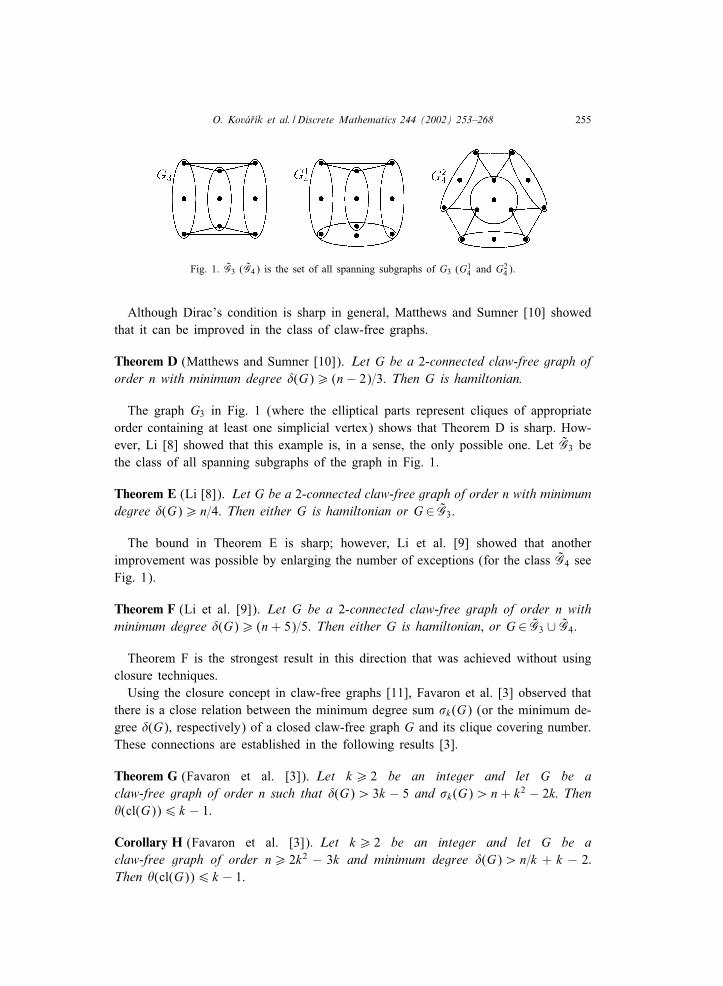
O. Kov�a!r��k et al. / Discrete Mathematics 244 (2002) 253–268 255
Fig. 1. G̃3 (G̃4) is the set of all spanning subgraphs of G3 (G14 and G2
4).
Although Dirac’s condition is sharp in general, Matthews and Sumner [10] showedthat it can be improved in the class of claw-free graphs.
Theorem D (Matthews and Sumner [10]). Let G be a 2-connected claw-free graph oforder n with minimum degree �(G)¿ (n− 2)=3. Then G is hamiltonian.
The graph G3 in Fig. 1 (where the elliptical parts represent cliques of appropriateorder containing at least one simplicial vertex) shows that Theorem D is sharp. How-ever, Li [8] showed that this example is, in a sense, the only possible one. Let G̃3 bethe class of all spanning subgraphs of the graph in Fig. 1.
Theorem E (Li [8]). Let G be a 2-connected claw-free graph of order n with minimumdegree �(G)¿ n=4. Then either G is hamiltonian or G ∈ G̃3.
The bound in Theorem E is sharp; however, Li et al. [9] showed that anotherimprovement was possible by enlarging the number of exceptions (for the class G̃4 seeFig. 1).
Theorem F (Li et al. [9]). Let G be a 2-connected claw-free graph of order n withminimum degree �(G)¿ (n+ 5)=5. Then either G is hamiltonian; or G ∈ G̃3 ∪ G̃4.
Theorem F is the strongest result in this direction that was achieved without usingclosure techniques.
Using the closure concept in claw-free graphs [11], Favaron et al. [3] observed thatthere is a close relation between the minimum degree sum �k(G) (or the minimum de-gree �(G), respectively) of a closed claw-free graph G and its clique covering number.These connections are established in the following results [3].
Theorem G (Favaron et al. [3]). Let k¿ 2 be an integer and let G be aclaw-free graph of order n such that �(G)¿ 3k − 5 and �k(G)¿n+ k2 − 2k: Then�(cl(G))6 k − 1.
Corollary H (Favaron et al. [3]). Let k¿ 2 be an integer and let G be aclaw-free graph of order n¿ 2k2 − 3k and minimum degree �(G)¿n=k + k − 2:Then �(cl(G))6 k − 1.
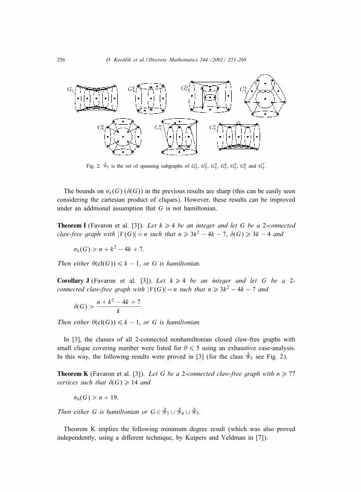
256 O. Kov�a!r��k et al. / Discrete Mathematics 244 (2002) 253–268
Fig. 2. G̃5 is the set of spanning subgraphs of G15 , G
25 , G
35 , G
45 , G
55 , G
65 and G7
5 .
The bounds on �k(G) (�(G)) in the previous results are sharp (this can be easily seenconsidering the cartesian product of cliques). However, these results can be improvedunder an additional assumption that G is not hamiltonian.
Theorem I (Favaron et al. [3]). Let k¿ 4 be an integer and let G be a 2-connectedclaw-free graph with |V (G)|= n such that n¿ 3k2 − 4k − 7, �(G)¿ 3k − 4 and
�k(G)¿n+ k2 − 4k + 7:
Then either �(cl(G))6 k − 1, or G is hamiltonian.
Corollary J (Favaron et al. [3]). Let k¿ 4 be an integer and let G be a 2-connected claw-free graph with |V (G)|= n such that n¿ 3k2 − 4k − 7 and
�(G)¿n+ k2 − 4k + 7
k:
Then either �(cl(G))6 k − 1, or G is hamiltonian.
In [3], the classes of all 2-connected nonhamiltonian closed claw-free graphs withsmall clique covering number were listed for �6 5 using an exhaustive case-analysis.In this way, the following results were proved in [3] (for the class G̃5 see Fig. 2).
Theorem K (Favaron et al. [3]). Let G be a 2-connected claw-free graph with n¿ 77vertices such that �(G)¿ 14 and
�6(G)¿n+ 19:
Then either G is hamiltonian or G ∈ G̃3 ∪ G̃4 ∪ G̃5.
Theorem K implies the following minimum degree result (which was also provedindependently, using a diRerent technique, by Kuipers and Veldman in [7]).
O. Kov�a!r��k et al. / Discrete Mathematics 244 (2002) 253–268 257
Corollary L (Favaron et al. [3], Kuipers and Veldman [7]). Let G be a 2-connectedclaw-free graph of order n¿ 78 with
�(G)¿n+ 16
6:
Then either G is hamiltonian or G ∈G3 ∪ G4 ∪ G5.
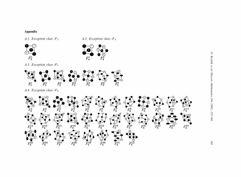
Let Fi (i= 3; : : : ; 7) be the classes of graphs listed in the appendix. For any Fji ∈Fi,let G
ji be the set of all spanning subgraphs of all graphs obtained from the line
graph L(Fji ) of Fji by adding an appropriate number of simplicial vertices to thosecliques of L(Fji ) that correspond to the black vertices of Fji , and set Gi =
⋃|Fi|−1j=0 G
ji ,
i= 3; : : : ; 7. Then it is easy to see that for i= 3; 4; 5, Gi = {cl(G) |G ∈ G̃i is 2-connectedand claw-free}, where G̃i (i= 3; 4; 5) are the classes of graphs from Figs. 1 and 2.
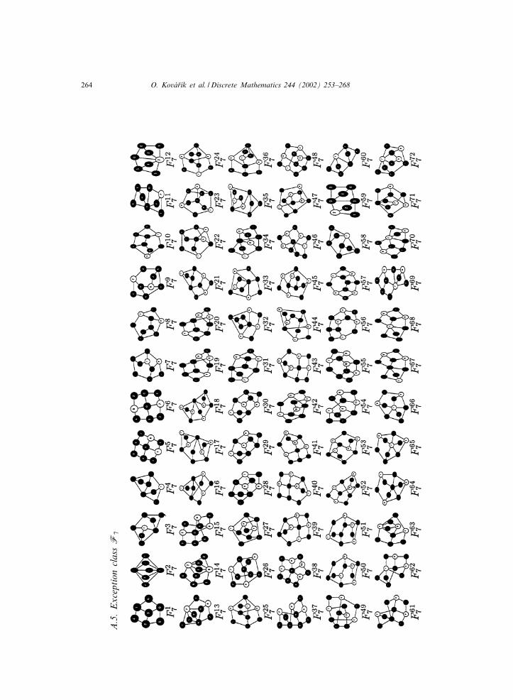
In Sections 3 and 4, we present a method that was used for <nding the classesF6 and F7 and establishing the fact that a 2-connected closed claw-free graph Gwith �(G)6 7 is nonhamiltonian if and only if G ∈⋃7
i=3 Gi. This result together withTheorem I and Corollary J yields the following theorem (which is the main result ofthis paper).
Theorem 1. Let G be a 2-connected claw-free graph of order n¿ 153 such that�(G)¿ 20 and
�8(G)¿n+ 39:
Then either G is hamiltonian or G ∈⋃7i=3 Gi.
Theorem 1 immediately implies the following minimum degree result.
Corollary 2. Let G be a 2-connected claw-free graph of order n¿ 153 with minimumdegree
�(G)¿n+ 39
8:
Then either G is hamiltonian or G ∈⋃7i=3 Gi.
The proof of Theorem 1 and Corollary 2 follows immediately from Theorem I andCorollary J, respectively, and from the above mentioned properties of the classes Fi.In the following sections, we present the method which was used for the computersearch for the classes of exceptions with �= 6; 7.
3. Preliminary observations
In this section, we present basic de<nitions, notation and some auxiliary statementsthat will ensure the correctness and <niteness of the algorithm presented in Section 4.

258 O. Kov�a!r��k et al. / Discrete Mathematics 244 (2002) 253–268
We basically follow the terminology and notation introduced in [3]. Let G� be theclass of all 2-connected nonhamiltonian closed claw-free graphs with clique coveringnumber �. By Theorem A, every G ∈G� is the line graph of some (unique) triangle-free graph H . Let D1(H) be the set of all degree 1 vertices of H and put H ′ =H − D1(H). Set H�= {L−1(G) |G ∈G�} and H′
�= {H − D1(H) |H ∈H�}. Sinceevery G ∈G� is 2-connected, every H ∈H� or H ′ ∈H′
� is essentially 2-edge-con-nected or 2-edge-connected, respectively.
In every G ∈G� choose a <xed minimum clique covering PG = {B1; : : : ; B�} ofG such that each clique Bi is maximal. Since PG is minimum, every Bi containsat least one proper vertex, i.e. a vertex belonging to no other clique of PG. Thecenters B1; : : : ; B� of the stars of H =L−1(G) that correspond to the cliques of Gwill be called the black vertices of H . The other vertices of H are called white.The set of black (white) vertices of H is denoted by B(H) (W (H)), respectively.Two vertices b1; b2 ∈B(H) are said to be related if they are either adjacent or theyhave a white common neighbor. Since B(H) is a vertex covering of H (i.e., ev-ery edge of H has at least one vertex in B(H)), the set W (H) isindependent.
It is easy to see that for any G ∈G�, any graph obtained from G by adding=removingsimplicial vertices to=from cliques of PG also belongs to G� as long as (in the case ofremoval) at least one simplicial vertex in the clique remains (while the removal of thelast simplicial vertex of a clique can turn G into a hamiltonian graph). Hence, we canwithout loss of generality denote for any H ′ ∈H′
� by L(H) the line graph of H ′ inwhich one simplicial vertex is added to every clique corresponding to a black vertexof H ′.
Let G1; G2 ∈G�. We say that G1 is an ss-subgraph of G2, if G1 is isomorphicto a spanning subgraph of a graph, which is obtained from G2 by adding an ap-propriate number of simplicial vertices to some cliques of PG2 , and that G1 is aproper ss-subgraph of G2 if G1 is an ss-subgraph of G2 and G1, G2 are noniso-morphic. In the following, we present a method for <nding a subset F� ⊂ H′
�such that
(i) every G ∈G� is an ss-subgraph of L(F) for some F ∈F�,(ii) for any F1; F2 ∈F�, L(F1) is not an ss-subgraph of L(F2).
By the previous observations, the class G� is fully characterized by F�.If, for some H ∈H�, the corresponding H ′ ∈H′
� has a black closed trail (BCT),i.e. a closed trail containing all black vertices of H ′, then clearly H has a DCT. Since,by Theorem B, no H ∈H� has a DCT, no H ′ ∈H′
� has a BCT.We say that a graph H ′ ∈H′
� is reducible if there is a graph H ′1 ∈H′
t for somet6 � such that either
(i) H ′1 is obtained from H ′ by adding a relation (i.e., an edge or a white common
neighbor) between two black vertices, or(ii) H ′
1 =H ′|Y for some Y ⊂ V (H ′) with |Y |¿ 2.

O. Kov�a!r��k et al. / Discrete Mathematics 244 (2002) 253–268 259
In the <rst case, we say that H ′ is r-reducible. In the second case, H ′ is said tobe ww-reducible if |Y ∩ B(H ′)|= 0, bw-reducible if |Y ∩ B(H ′)|= 1, bb-reducible if|Y ∩ B(H ′)|¿ 2.
The following statement shows that reducibility in H′� is closely linked with
ss-subgraphs in G�.
Theorem 3. Let G ∈G�, H =L−1(G)∈H� and H ′ =H − D1(H)∈H′�. Then H ′ is
reducible if and only if there is a graph G1 ∈Gt (for some t6 �) such that G is aproper ss-subgraph of G1.
Proof. 1. Suppose <rst that H ′ is reducible. If H ′1 is obtained by adding a relation
between bi; bj ∈B(H ′), then L(H ′1) is obtained from L(H ′) either by adding a new
vertex and joining it with all vertices of Bi and Bj (where Bi and Bj are the cliquescorresponding to bi and bj) if an edge is added, or by adding a simplicial vertex toeach of Bi, Bj and joining these vertices with an edge, if a relation with a new whitevertex was added. In both cases, L(H) is a proper ss-subgraph of L(H ′
1).Let H ′
1 =H ′|Y for a set Y ⊂ V (H ′) with |Y |¿ 2. Denote by YE the set of edges of H ′
that have at least one vertex in Y and by Y ′E the corresponding set of vertices of L(H ′).
Then L(H ′1) can be equivalently obtained from L(H ′) by adding all missing edges with
both vertices in Y ′E (i.e., by making 〈Y ′
E〉 a clique) and then removing an appropriatenumber of simplicial vertices. Thus, L(H) is again a proper ss-subgraph of L(H ′
1).2. Let now G be a proper ss-subgraph of some G1 ∈Gt , t6 �. Then G is a spanning
subgraph of a graph GS1 ∈Gt , where GS1 was obtained from G1 by adding simplicialvertices to cliques of PG. Clearly also GS1 ∈Gt ; hence we can suppose GS1 =G1.
Let uv∈E(G1)\E(G). Since PG is a clique covering of G, there are cliquesBu; Bv ∈PG such that u∈Bu\Bv and v∈Bv\Bu. Let bu; bv be the corresponding blackvertices in H ′.
First suppose that there is a vertex z ∈Bu∩Bv. Then, since {u; v; z} induces a triangleand G1 is closed, 〈Bu∪Bv〉G1 is a clique. Hence H is bb-reducible (with Y = {bu; bv}).Thus, in the sequel we can suppose that Bu ∩ Bv= ∅. We distinguish several cases.
Case 1: Both u and v are simplicial in G. Then adding uv corresponds in H toadding a relation b1wb2, where w is a (new) white vertex. Hence H is r- reducible.
Case 2: One of u, v is not simplicial in G. By symmetry, suppose v is simplicialand u is not. Then u∈Ku for some clique Ku ⊂ V (G), Bu =Ku =Bv. Let zu ∈V (H ′) bethe vertex corresponding to Ku. If Ku ∩Bv = ∅, then, since G1 is closed, 〈Ku ∪Bv〉G1 isa clique, implying H ′ is bw- or bb-reducible with Y = {zu; bv} (depending on whetherzu is white or black in H ′). If Ku ∩ Bv= ∅, then, since u cannot be a center of a clawin G1, we have the following three possibilities.
• 〈Bu ∪ {v}〉G1 is a clique. Then H ′ is r-reducible with adding the edge bubv.• 〈Ku ∪{v}〉G1 is a clique. Then similarly H ′ is r-reducible with adding the edge zubv
(and hence, if zu is white, the relation buzubv).• 〈Ku ∪ Bu}〉G1 is a clique. Then even the graph, obtained from G just by making〈Ku ∪ Bu}〉G1 a clique (i.e. without adding uv) also belongs to Gt , implying that
260 O. Kov�a!r��k et al. / Discrete Mathematics 244 (2002) 253–268
H ′ is bb- or bw-reducible with Y = {bu; zu} (depending on whether zu is black orwhite). The possibility of adding the edge uv then yields r-reducibility by Case 1.
Case 3: Neither u nor v is simplicial in G. Then v∈Kv for some clique Kv diRerentfrom Ku; Bu; Bv. It is straightforward to check that, since neither u nor v can be a centerof a claw, some two of the cliques Ku; Kv; Bu; Bv induce one clique, implying that H ′
is reducible.
4. Algorithm
In this section, we present the general idea of the algorithm used for generatingall graphs from the classes F6 and F7. We do not give all technical details ofthe implementation. The interested reader can <nd this information in the Thesis [6]which is (with the complete version of the source code of the program) availableon www.
By Theorem 3, we have F�= {F ∈H′� |F is ireducible}. For any closed trail T in
a graph F ∈F�, denote by bla(T ) the number of black vertices of T and by blo(T )the number of blocks of T . In every F ∈F� choose a closed trail TF such that, amongall closed trails in F ,
(i) bla(TF) is maximum,(ii) subject to (i), blo(TF) is minimum,(iii) subject to (i) and (ii), TF has minimum number of edges.
Such a TF clearly exists and, since F has no BCT, bla(TF)¡�. Hence every F ∈F�
consists of the trail TF with properties (i)–(iii), some black vertices outside TF andsome additional relations. This gives the following general idea of an algorithm for<nding all graphs from the class F�.
Step 1. Generate all minimal closed trails T with bla(T )¡�.Step 2. For each closed trail T from Step 1, generate all minimal 2-edge-connected
graphs T 1, consisting of the trail T , additional � − bla(T ) black vertices andconnecting relations.
Step 3. Check each of the graphs T 1 from Step 2 for bb-reducibility. If T 1 is notbb-reducible, keep it (as T 2) for Step 4; otherwise generate all graphs T 2
obtained from T1 by adding a minimal set of relations such that T 2 is notbb-reducible.
Step 4. (a) For each of the graphs T 2 from Step 3, generate all graphs T 2a , obtained
from T 2 by adding all possible sets of relations that do not imply the exis-tence of a closed trail T ′ with bla(T ′)¿ bla(T ) or with bla(T ′) = bla(T ) andblo(T ′)¡ blo(T ).(b) For each of the graphs T 2
a from Step 4a, create all possible graphs T 2b by
replacing by an edge all relations containing a white vertex of degree 2 forwhich the replacement does not yield a triangle.
O. Kov�a!r��k et al. / Discrete Mathematics 244 (2002) 253–268 261
Step 5. Check each of the graphs T 2b from Step 4b for reducibility. F� is the set of
all ireducible graphs T 2b .
In Step 1, for the considerations that follow, suppose without loss of generality thatthe generated minimal trails T are ordered in the order suggested by the preferences ofthe choice of TF , i.e. in nonincreasing order of bla(T ) and, for each value of bla(T ),in nondecreasing order of blo(T ).
In Step 2, the graphs T 1 are generated, for any <xed closed trail T from Step 1, bychecking all possible relations between T and the vertices outside T . In order to reducethe number of cases to be considered, each of these graphs is checked for minimality(this can be supposed without loss of generality since the possibly missed relations areadded later on in Step 4 anyway).
In Step 3, bb-reducibility of T 1 means that L(T 1) is an ss-subgraph of a graph fromFt for some t ¡�, i.e. it is already known. However, this bb-reducibility can be dueto some missing relations, and not considering this possibility could result in missingsome cases.
In all steps from Step 1 to Step 4a, all relations are supposed to contain a whitevertex (this can be supposed without loss of generality since the white vertices whichdo not yield any new case are removed in Step 4b anyway).
In Step 4c, all further relations are added.In all steps, the constructed graphs are checked for isomorphism with the previously
generated (and stored) graphs.In Steps 2–4, all constructed graphs are checked for nonexistence of a closed trail
T ′ such that bla(T ′)¿ bla(T ) or bla(T ′) = bla(T ) and blo(T ′)¡ blo(T ) (where T isthe closed trail that the graph under consideration was obtained from) since otherwisethe subcase can be transformed to some of the previous ones. All constructed graphsare of course checked for being triangle-free.
It is clear that the algorithm, if it stops, yields all ireducible 2-edge-connectedtriangle-free graphs covered by a set of � black vertices and with no BCT, i.e., byProposition 3, the class F�.
Kuipers and Veldman [7] proved that, for each �¿ 0, the set F� is <nite (using adiRerent, nonalgorithmic approach). Thus, to establish the <niteness of the algorithm, itsuSces to show that the method used for generating closed trails in Step 1 always halts.
Let t be an integer and let T be a closed trail containing a covering set of bla(T ) = tblack vertices. Suppose that T is minimal (i.e., no proper subtrail of T contains allits black vertices). Let CT be a cycle such that T is obtained from CT by a se-ries of identi<catons of some of its vertices of the same color. For any i¿ 1 de-note by mi(T ) the number of black vertices of T that the trail T passes throughi-times (i.e., the number of black vertices of degree 2i). Then we have the followingstatement.
Theorem 4. Let t be an integer and let T be a minimal closed trail with bla(T ) = t. Then
(i) m1(T ) + m2(T ) + · · ·= bla(T ),
262 O. Kov�a!r��k et al. / Discrete Mathematics 244 (2002) 253–268
(ii) if mj(T ) = 0 for some j¿ 2, then m1(T )¿ j,(iii) mj(T ) = 0 for j¿ t,(iv) CT has at most 1
4 (t + 1)2 black vertices.
Remark. Part (iv) of Theorem 4 establishes <niteness of Step 1 of the algorithm.
Proof. (i) Part (i) is straightforward.(ii) Let mj(T ) = 0, let y be a vertex of T with degree 2j and suppose that y is
obtained by identifying vertices x1; : : : ; xj (j¿ 2) of CT . If m1(T )¡j, then, in someof the segments of CT between two consecutive xi’s (say, in x1CTx2), all interior blackvertices are identi<ed in T with some other vertices. But then the cycle (x1 = x2)CTx1(obtained from CT by identifying x1 with x2 and removing all interior vertices ofthe segment x1CTx2) yields a shorter trail T ′ with bla(T ′) = bla(T ), contradicting theminimality of T .
(iii) If mj(T ) = 0 for some j¿ t, then, by (ii), m1(T )¿ j, implying t¿m1 +m2 +· · · + mj¿m1 + mj¿ j + 1¿ t + 1, a contradiction.
(iv) Let m= max{j¿ 1 |mj(T ) = 0}. By (iii), m6 t − 1, and by (ii), m1(T )¿m.Hence at least m black vertices of T have degree 2, and the remaining at most t − mblack vertices of T have degree at most 2m. This implies bla(CT ) ≤ 1m+m(t−m) =−m2 + (t + 1)m= (t + 1)2=4 − (m− t + 1=2)26 (t + 1)2=4.
Concluding remarks: 1. The algorithm was implemented in parallel on a cluster of6 parallel workstations (6× Pentium Xeon 450 MHz, 6× 256 MB RAM, interconnec-tion 1; 6 Gb=s), running MPI (Message passing interface). A nonparallel version of thealgorithm was also developed and implemented. The computing time of the parallelversion was approx. 1 min for �= 6 and 107 min for �= 7.
2. Generally speaking, it could be possible to obtain the exception classes even forlarger values of �. Nevertheless, the authors are convinced that a result presenting a de-gree condition for hamiltonicity in 2-connected claw-free graphs of type �9(G)¿n+52(or, as a corollary, �(G)¿ (n+ 52)=9) with a book of exceptions probably would notbe very useful (although some of the exceptional graphs could be of interest on theirown right). Thus, the authors believe that in the chase of improvements of degree con-ditions for hamiltonicity in 2-connected claw-free graphs there not much remains tobe done.
Acknowledgements
The cluster used for the computation was built under a project M%SMT No. LB98246“Lyra”.
O.
Kov �a !r ��k
etal./D
iscreteM
athematics
244(2002)
253–268263
Appendix
A.1. Exception class F3 A.2. Exception class F4
A.3. Exception class F5
A.4. Exception class F6
264 O. Kov�a!r��k et al. / Discrete Mathematics 244 (2002) 253–268
A.5
.E
xcep
tion
clas
sF
7
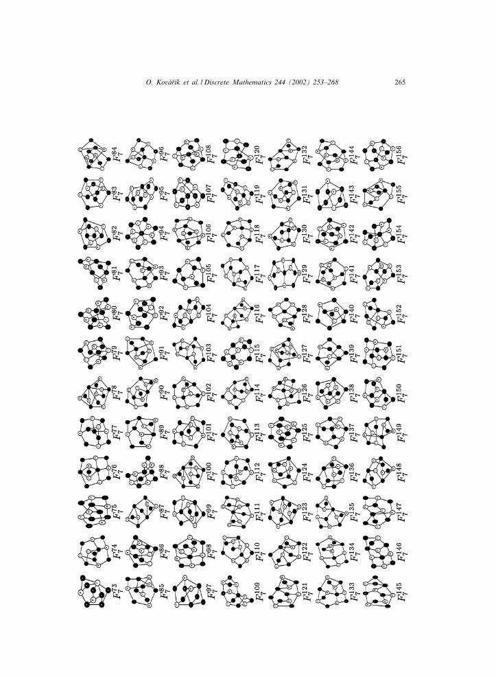
O. Kov�a!r��k et al. / Discrete Mathematics 244 (2002) 253–268 265
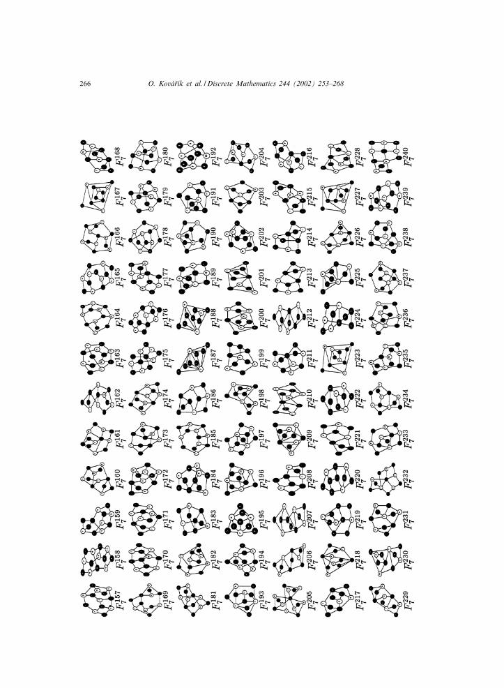
266 O. Kov�a!r��k et al. / Discrete Mathematics 244 (2002) 253–268

O. Kov�a!r��k et al. / Discrete Mathematics 244 (2002) 253–268 267
268 O. Kov�a!r��k et al. / Discrete Mathematics 244 (2002) 253–268
References
[1] J.A. Bondy, U.S.R. Murty, Graph Theory with Applications, Macmillan, London and Elsevier, NewYork, 1976.
[2] G.A. Dirac, Some theorems on abstract graphs, Proc. London Math. Soc. 2 (1952) 69–81.[3] O. Favaron, E. Flandrin, H. Li, Z. Ryj(a%cek, Clique covering and degree conditions for hamiltonicity in
claw-free graphs, Discrete Math. 236 (2001) 65–80.[4] R. Faudree, E. Flandrin, Z. Ryj(a%cek, Claw-free graphs—a survey, Discrete Math. 164 (1997) 87–147.[5] F. Harary, C. St.J.A. Nash-Williams, On eulerian and hamiltonian graphs and line graphs, Canad. Math.
Bull. 8 (1965) 701–709.[6] O. Kov(a%r()k, M. Mula%c, Nonhamiltonian closed claw-free graphs with small clique covering number.
M.Sc. Thesis, University of West Bohemia, Pilsen, 1999; http:==lyra.zcu.cz=papers=.[7] E.J. Kuipers, H.J. Veldman, Recognizing claw-free hamiltonian graphs with large minimum degree,
Preprint 1998, submitted for publication.[8] H. Li, Hamiltonian cycles in 2-connected claw-free graphs, J. Graph Theory 20 (1995) 447–457.[9] H. Li, M. Lu, F. Tian, B. Wei, Hamiltonian cycles in claw-free graphs with at most 5�-5 vertices,
Congr. Numer. 122 (1996) 184–202.[10] M.M. Matthews, D.P. Sumner, Longest paths and cycles in K1;3-free graphs, J. Graph Theory 9 (1985)
169–177.[11] Z. Ryj(a%cek, On a closure concept in claw-free graphs, J. Combin. Theory Ser. B 70 (1997) 217–224.