A nonlinear position and attitude observer on SE(3) using landmark measurements

This article appeared in a journal published by Elsevier. The attachedcopy is furnished to the author for internal non-commercial researchand education use, including for instruction at the authors institution

and sharing with colleagues.

Other uses, including reproduction and distribution, or selling orlicensing copies, or posting to personal, institutional or third party

websites are prohibited.

In most cases authors are permitted to post their version of thearticle (e.g. in Word or Tex form) to their personal website orinstitutional repository. Authors requiring further information

regarding Elsevier’s archiving and manuscript policies areencouraged to visit:

http://www.elsevier.com/copyright

http://www.elsevier.com/copyright

Author's personal copy

Systems & Control Letters 59 (2010) 155–166

Contents lists available at ScienceDirect

Systems & Control Letters

journal homepage: www.elsevier.com/locate/sysconle

A nonlinear position and attitude observer on SE(3) usinglandmark measurementsJ.F. Vasconcelos, R. Cunha ∗, C. Silvestre, P. OliveiraInstitute for Systems and Robotics, Instituto Superior Técnico, 1046-001 Lisbon, Portugal

a r t i c l e i n f o

Article history:Received 23 June 2009Received in revised form13 November 2009Accepted 13 November 2009Available online 1 February 2010

Keywords:Nonlinear observerLyapunov stabilityBias filteringExponential convergenceLinear time-varying systems

a b s t r a c t

This paper addresses the problem of position and attitude estimation, based on landmark readings andvelocity measurements. A derivation of a nonlinear observer on SE(3) is presented, using a Lyapunovfunction conveniently expressed as a function of the difference between the estimated and the measuredlandmark coordinates. The resulting feedback laws are explicit functions of the landmark measurementsand velocity readings, exploiting the sensor information directly in the observer. The proposed observeryields almost global asymptotic stabilization of the position and attitude errors and exponentialconvergence in any closed ball inside the region of attraction. Also, it is shown that the asymptoticconvergence of the estimation error trajectories is shaped by the landmark geometry and observer designparameters. The problem of non-ideal velocity readings is also considered, and the observer is augmentedto compensate for bias in the angular and linear velocity measurements. The resulting position, attitude,and bias estimation errors are shown to converge exponentially fast to the desired equilibrium points,for bounded initial estimation errors. Simulation results are presented to illustrate the stability andconvergence properties of the observer.

© 2009 Elsevier B.V. All rights reserved.

1. Introduction

Landmark-based navigation is recognized as a promising strat-egy for providing autonomous vehicles with accurate position andattitude information during critical operation stages such as take-off, landing, or docking. Among a wide diversity of suitable esti-mation techniques, nonlinear observers stand out as an excitingapproach often endowed with stability results [1], and formulatedrigorously in non-Euclidean spaces. Research on the problemof de-riving a stabilizing law for systems evolving on manifolds, suchas SO(3) and SE(3), can be found in [2–8], where the topologicallimitations for achieving global stabilization on SO(3) provide im-portant guidelines for the design of observers. In particular, theselimitations call for the relaxation from global to almost global sta-bility, as adopted in [9,10], meaning that the region of attraction ofthe origin comprises all the state space except a nowhere dense setof measure zero [11].Nonlinear attitude and position observers, with application to

aerospace, terrestrial and oceanic vehicles, have been proposed in

∗ Corresponding address: Institute for Systems and Robotics (ISR), InstitutoSuperior Técnico (IST), Avenue Rovisco Pais, 1, Torre Norte, 8 Andar, 1049-001,Lisbon, Portugal. Tel.: +351 21 8418090; fax: +351 21 8418291.E-mail addresses: [email protected] (J.F. Vasconcelos),

[email protected] (R. Cunha), [email protected] (C. Silvestre), [email protected](P. Oliveira).

recent literature. A seminal work on nonlinear attitude observerscan be found in [12], where the author proposes a solution toestimate the attitude in the Euler quaternion representation, usingattitude and torque measurements. Subsequent work has beendevoted to nonlinear observers based on the attitude and positionkinematics [13–17], which can be implemented on any roboticplatform, irrespective of its dynamics. Somemethodologies for thedesign of kinematic observers evolving on manifolds have beenput forth in [7,11,18,19]. Another line of work has been directedat the design of nonlinear observers that exploit informationsources adopted in classical navigation problems [15–17,20], andcompensate for non-ideal sensor readings that have long beenconsidered in filtering estimation techniques.This work explores the circle of ideas found in [19,21], which

were proposed to address the problem of rigid-body stabilizationbased on landmark measurements and ideal velocity readings. Inthis paper, the problem of attitude and position estimation onSE(3) is addressed and a nonlinear observer based on landmarkmeasurements and possibly biased velocity readings is proposed.The observer is derived constructively using a convenientlydefined Lyapunov function, defined by the landmark estimationerror. For ideal velocity readings, the obtained feedback law yieldsalmost global asymptotic stability of the desired equilibrium pointon SE(3), and exponential convergence of the attitude and positionestimates in any closed ball inside the region of attraction.The adopted derivation technique yields feedback laws that are

an explicit function of the sensor measurements. The direct use

0167-6911/$ – see front matter© 2009 Elsevier B.V. All rights reserved.doi:10.1016/j.sysconle.2009.11.008


156 J.F. Vasconcelos et al. / Systems & Control Letters 59 (2010) 155–166

of sensor readings in the feedback law provides for a geometricinsight on the observer properties. Namely, it shows that theasymptotic behavior of the estimation errors can be shaped byjudicious landmark placement and design parameter tuning. Also,it highlights the necessary landmark configuration for attitude andposition estimation.The problem of bias in the velocity readings is addressed by

extending the proposed observer to dynamically compensate forthese sensor non-idealities. Exponential stabilization of the po-sition and attitude estimation errors is obtained, for worst-caseinitial estimation errors. Recent results for parameterized lineartime-varying systems [22] are adopted in the stability analysis ofthe system. Simulation results validate the proposed observer, andillustrate the derived properties. A preliminary version of thisworkhas been presented in [23].The paper is organized as follows. In Section 2, the position

and attitude estimation problem is introduced and the availablesensor information is detailed. The attitude and position observeris derived in Section 3. A convenient landmark-based Lyapunovfunction is defined, and the necessary and sufficient landmarkconfiguration for attitude estimation is discussed. Almost globalstabilizing feedback laws are obtained for attitude and positionestimation. The resulting observer dynamics are expressed as afunction of the sensor readings, and it is shown that the asymptoticconvergence of the system trajectories is determined by thelandmark geometry, and by the design parameters. The problem ofunknown velocity sensor bias is studied in Section 4. The observerdynamics are extended to dynamically compensate for the biasin the linear and angular velocity measurements, and stabilityresults are derived. In Section 5, simulation results illustrate theobserver properties for time-varying linear and angular velocities.Concluding remarks are presented in Section 6.

Nomenclature

The notation adopted is fairly standard. Column vectors andmatrices are denoted respectively by lowercase and uppercaseboldface type, e.g. s and S. The transpose of a vector or matrix willbe indicated by a prime, e.g. s′ and S′. The set of n × m matriceswith real entries is denoted by M(n,m) and M(n) := M(n, n).The sets of orthogonal, special orthogonal, symmetric, and skew-symmetricmatrices are denoted byO(n) := U ∈ M(n) : U′U = I,SO(n) := R ∈ O(n) : det(R) = 1, L(n) := S ∈ M(n) : S = S′,and so(n) := S ∈ M(n) : S = −S′, respectively. The specialEuclidean group is given by the product space of SO(n) with Rn,SE(n) := SO(n)× Rn [24]. The n-dimensional unit sphere and ballare described by S(n) := x ∈ Rn+1 : x′x = 1 and B(n) := x ∈Rn : x′x ≤ 1, respectively. The operator (a)× : R3 → so(3)yields the skew-symmetric matrix defined by the vector a ∈ R3such that (a)× b = a× b, b ∈ R3. The inverse of (·)× is denoted by(·)⊗, i.e.

((a)×

)⊗= a.

2. Problem formulation

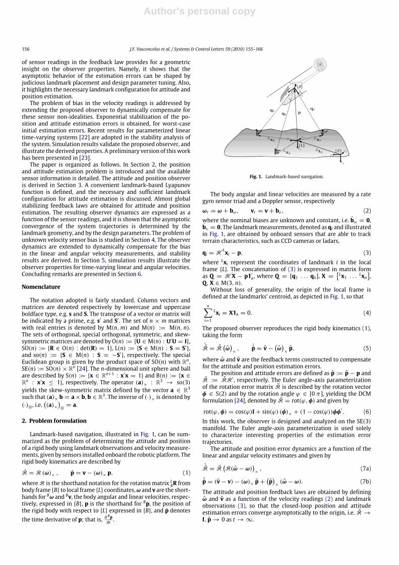
Landmark-based navigation, illustrated in Fig. 1, can be sum-marized as the problem of determining the attitude and positionof a rigid body using landmark observations and velocity measure-ments, given by sensors installed onboard the robotic platform. Therigid body kinematics are described by

R = R (ω)× , p = v− (ω)× p, (1)

whereR is the shorthand notation for the rotation matrix LBR frombody frame B to local frame L coordinates,ω and v are the short-hands for Bω and Bv, the body angular and linear velocities, respec-tively, expressed in B, p is the shorthand for Bp, the position ofthe rigid body with respect to L expressed in B, and p denotesthe time derivative of p; that is, d

Bpdt .

Fig. 1. Landmark-based navigation.

The body angular and linear velocities are measured by a rategyro sensor triad and a Doppler sensor, respectively

ωr = ω + bω, vr = v+ bv, (2)

where the nominal biases are unknown and constant, i.e. bω = 0,bv = 0. The landmarkmeasurements, denoted as qi and illustratedin Fig. 1, are obtained by onboard sensors that are able to trackterrain characteristics, such as CCD cameras or ladars,

qi = R′Lxi − p, (3)

where Lxi represent the coordinates of landmark i in the localframe L. The concatenation of (3) is expressed in matrix formas Q = R′X − p1′n, where Q = [q1 . . . qn], X =

[Lx1 . . . Lxn

],

Q,X ∈ M(3, n).Without loss of generality, the origin of the local frame is

defined at the landmarks’ centroid, as depicted in Fig. 1, so thatn∑i=1

Lxi = X1n = 0. (4)

The proposed observer reproduces the rigid body kinematics (1),taking the form

˙R = R(ω)×, ˙p = v−

(ω)×p, (5)

where ω and v are the feedback terms constructed to compensatefor the attitude and position estimation errors.The position and attitude errors are defined as p := p − p and

R := RR′, respectively. The Euler angle-axis parameterizationof the rotation error matrix R is described by the rotation vectorφ ∈ S(2) and by the rotation angle ϕ ∈ [0 π ], yielding the DCMformulation [24], denoted by R = rot(ϕ,φ) and given by

rot(ϕ,φ) = cos(ϕ)I+ sin(ϕ) (φ)× + (1− cos(ϕ))φφ′. (6)

In this work, the observer is designed and analyzed on the SE(3)manifold. The Euler angle-axis parameterization is used solelyto characterize interesting properties of the estimation errortrajectories.The attitude and position error dynamics are a function of the

linear and angular velocity estimates and given by

˙R = R(R(ω − ω)

)×, (7a)

˙p = (v− v)− (ω)× p+(p)×(ω − ω). (7b)

The attitude and position feedback laws are obtained by definingω and v as a function of the velocity readings (2) and landmarkobservations (3), so that the closed-loop position and attitudeestimation errors converge asymptotically to the origin, i.e. R →I, p→ 0 as t →∞.


J.F. Vasconcelos et al. / Systems & Control Letters 59 (2010) 155–166 157

The attitude and position feedback laws are derived first for thecase of unbiased velocity measurements (bω = bv = 0), and thecase of biased linear and angular velocity measurements (bω, bvunknown) is subsequently considered.

3. Observer synthesis with ideal velocity measurements

In this section, the attitude and position feedback laws arederived for the case of ideal angular and linear velocity measure-ments, where bω = bv = 0. The closed-loop system is demon-strated to have an almost GAS equilibrium point at (R, p) = (I, 0),which is exponentially stable in any closed ball inside the region ofattraction.Some relevant characteristics of the observer are pointed out.

It is shown that the position and attitude feedback laws can beexpressed as an explicit function of the sensor readings, allowingfor the observer implementation in practice. Also, the asymptoticbehavior of the attitude observer trajectories is studied in the Eulerangle-axis representation, characterizing the directionality of theobserver estimates given the design feedback law.

3.1. Landmark-based Lyapunov function

The observer is derived resorting to Lyapunov’s stability theory.To exploit the landmark readings information, vector and positionmeasurements are constructed from a linear combination of (3),producing respectively

Buj =n−1∑i=1

aij(qi+1 − qi), Bun = −1n

n∑i=1

qi, (8)

where j = 1, . . . , n − 1. The transformation (8) can be expressedin matrix form asBU = QDA, Bun = Qdp, (9)

where BU =[Bu1 . . . Bun−1

]∈ M(3, n − 1), D =

[01×n−1In−1

]−[

In−101×n−1

], D ∈ M(n, n − 1), dp = −

1n1n, and the linear

transformation A = [aij] ∈ M(n − 1) is considered invertible byconstruction.Using the fact that 1′nD = 0, and that (4) implies Xdp = 0, (9)

can be rewritten asBU = R′U, Bun = p,where U = XDA. Consequently, BU and Bun can be reconstructedusing the observer estimates as follows:BU = R′U, Bun = p, (10)

which can be partitioned in columns BU =[Bu1 . . . Bun−1

], and

U =[Lu1 . . . Lun−1

].

The candidate Lyapunov function is defined by the estimationerror of the transformed vectors

V =12

n∑i=1

‖Bui − Bui‖2, (11)

which can be described as a sum of distinct position and attitudecomponents.

Proposition 1. The Lyapunov function (11) can be written as V =VR + Vp, where the distinct attitude and position components arerespectively given by

VR = tr[(I− R)UU′

]=14‖I− R‖2φ′Pφ, (12a)

Vp =12p′p (12b)

and P = tr(UU′)I− UU′.

Proof. The decoupling is obtained by defining the attitude andposition components as

VR =12

n−1∑i=1

‖Bui − Bui‖2, Vp =

12‖Bun − Bun‖2 (13)

producing V = VR + Vp immediately from (11).The attitude component is expressed as a function of the atti-

tude error by rewriting VR as

VR =12‖BU− BU‖2 =

12‖(R′ −R′)U‖2

=12‖(I− R)U‖2 =

12tr[(I− R)′UU′(I− R)

].

Using the trace properties presented in Appendix A and the DCMexpansion (6) yields

VR = tr[(I− R)UU′

]= tr

[(1− cos(ϕ))(I− φφ′)UU′

]= (1− cos(ϕ))φ′(tr(UU′)I− UU′)φ.

Using‖I−R‖2 = 4(1−cos(ϕ)) and thedefinition ofPproduces thedesired result. The formulation of Vp is obtained directly by notingthat Bun − Bun = p− p = p.

The time derivative of the Lyapunov function along the systemtrajectories is presented in the following statement.

Lemma 2. The time derivatives of proposed Lyapunov functions(12a) and (12b) are respectively given by

VR =(UU′R − R′UU′

)′⊗

R(ω − ω) (14a)

Vp = p′((

p)×(ω − ω)+ (v− v)

). (14b)

Proof. Differentiating the Lyapunov function (12b) with respectto time and using (7b) and p′ (ω)× p = 0 yields (14b) directly.Differentiating the Lyapunov function (12a) with respect to timeand using (7a) yields

VR = − tr( ˙RUU′) = − tr((R(ω − ω)

)×UU′R).

Using the properties of the trace, presented in Appendix A,produces

VR = −12tr((R(ω − ω)

)×(UU′R − R′UU′))

=(UU′R − R′UU′

)′⊗

R(ω − ω).

The decoupling property of the Lyapunov function allows forthe attitude and position estimation problems to be addressedseparately. The feedback law for the attitude kinematics (7a) isderived using the Lyapunov function VR , while the feedback lawfor the position kinematics (7b) relies on Vp.

3.2. Attitude feedback law

The attitude feedback law, derived in this section, exploits an-gular velocity sensors and landmarkmeasurements.While velocitysensors allow for the propagation of attitude in time, attitude withrespect to a reference frame is observed only bymeans of the land-markmeasurements. The geometric placement of the landmarks isrequired to satisfy the following assumption.

Assumption 1 (Landmark Configuration). The landmarks are not allcollinear; that is, rank(X) ≥ 2.Assumption 1 specifies the necessary and sufficient landmark

configuration under which zero observation error is equivalent tocorrect attitude estimation, i.e. ∀i=1..n−1‖Bui − Bui‖ = 0 ⇔ R= I. This is shown in the following proposition, using the fact that



the Lyapunov function VR expresses the estimation error of thetransformed landmarks.

Lemma 3. The Lyapunov function VR , expressed in (12a), has aunique global minimum (at R = I) if and only if Assumption 1 isverified.

Proof. From (13), it is straightforward that VR ≥ 0. From (12a),the zeros of VR are ϕ = 0 or φ ∈ N (P). To show that P > 0 ifand only if rank(X) ≥ 2, denote the singular value decompositionof U as U = UUSUV′U , where UU ∈ O(3), VU ∈ O(n), the off-diagonal elements of SU ∈ M(3, n) are zero (∀i6=jsij = 0) and thediagonal elements are the singular values of U, i.e. sii = σi(U),i ∈ 1, 2, 3. Then P = tr(UUU′U)I− UUU′U = tr(S

2U)I− UUS2UU

′

U =

UU

[s222 + s

233 0 0

0 s211 + s233 0

0 0 s211 + s222

]U′U and hence P > 0 if and only

if s22, s33 6= 0, i.e. rank(U) ≥ 2. Given that A and[D 1n

]are non-singular, the equality rank(U) = rank

([U 03

])=

rank(X[D 1n

] [ A 0n−10′n−1 1

])= rank(X), completes the proof.

Remark 1. It is instructive to analyze why a landmark configura-tion given by rank(X) = 1 is not sufficient to determine the atti-tude of the rigid body. If all Lxi are collinear, then all Lui are collinearand any R = rot(ϕ, Lui/‖Lui‖) satisfies Bui = Bui, i.e. the esti-mated and observed landmarks are identical for some R 6= R.This is related to the well known fact that a single vector observa-tion (such as the Earth’smagnetic field) yields attitude informationexcept for the rotation about the vector itself [25,26].

Given the Lyapunov function derivatives along the systemtrajectories (12a), consider the following feedback law:

ω = ωr − kωsω, (15)

where the feedback term is given by

sω = R′(UU′R − R′UU′

)⊗, (16)

and kω is a positive scalar. The attitude feedback yields theautonomous attitude error dynamics

˙R = −kωR(UU′R − R′UU′), (17)

and a negative semi-definite derivative for VR given by VR =

−kωs′ωsω ≤ 0. The set where VR = 0 is characterized in thefollowing lemma.

Lemma 4. Under Assumption 1, the set of points where VR = 0 isgiven by

CVR = R ∈ SO(3) : R = I ∨ R = rot(π,φ ∈ eigvec(P)).

Proof. The points where VR = 0 are given by sω = 0. UsingLemma 14 presented in Appendix A, sω can be rewritten as sω =Q′(ϕ,φ)Pφ. The points where sω = 0 satisfy Pφ ∈ N (Q′(ϕ,φ)),which is equivalent to

sin(ϕ)Pφ − (1− cos(ϕ)) (φ)× Pφ = 0.

For any x ∈ R3, x and (φ)× x are non-collinear, and henceQ′(ϕ,φ)Pφ = 0 if and only if ϕ = 0 or ϕ = π . For the ϕ = π case,the equality (φ)× Pφ = 0 is verified if and only if ∃αPφ = αφ.Consequently, VR = 0 if and only if ϕ = 0 ∨ (ϕ = π ∧ φ ∈eigvec(P)).

The open-loop dynamics of the Euler angle-axis representa-tion [27] are given by

ϕ = φ′R(ω − ω), φ =12

(I−

sin(ϕ)1− cos(ϕ)

(φ)×

)(φ)×R(ω − ω).

Using (15), the closed-loop dynamics can be written as

ϕ = −kω sin(ϕ)φ′Pφ, (18a)

φ = kω (φ)× (φ)× Pφ, (18b)

where the dynamics of φ are autonomous.Evaluating the closed-loop dynamics (18) for the points con-

tained in CVR shows that this set is invariant, which implies thatthe origin cannot be GAS. The existence of equilibrium points atϕ = π illustrates the topological obstacles to global stabiliza-tion when using continuous state feedback for systems defined onmanifolds. As discussed in [2,5,6], the region of attraction of a sta-ble equilibrium point is homeomorphic to some Euclidean vectorspace, which precludes global stabilization of the origin on SO(3).However, the notion of global asymptotic stability can be

relaxed by adopting the definition of almost global asymptotic sta-bility (aGAS) [9], in the sense that any trajectory emanating fromoutside a nowhere dense set of measure zero is attracted to theorigin. In the present case, the convergence to the origin R = Ifor all initial conditions outside the set ϕ = π can be estab-lished. Using the distance on SO(3) inherited by the Euclideannorm, d(R1,R2) = ‖R1−R2‖, the following theorem shows thatthe origin is aGAS and that the trajectories converge exponentiallyfast to the desired equilibrium point.

Theorem 5. The attitude error R = I of the closed-loop system (17)is aGAS and exponentially stable in any closed ball inside the region ofattraction, which is given by

RA = R ∈ SO(3) : ‖I− R‖2 < 8= (ϕ,φ) ∈ Dφ : ϕ < π

where Dφ = [0 π ] × S(2). For any R(t0) ∈ RA, the solution of thesystem (17) satisfies

‖R(t)− I‖ ≤ ‖R(t0)− I‖e−12 γR(t−t0), (19)

where γR =kω4 (8−‖R(t0)−I‖2)σ3(P) = kω(1+cos(ϕ(t0)))σ3(P).

Proof. Define the Lyapunov function

WR =‖I− R‖2

8=1− cos(ϕ)

2. (20)

The time derivative ofWR along the trajectories of the system (17)is described by

WR = −kω‖I− R‖2

8(8− ‖I− R‖2)

4φ′Pφ.

Using P > 0, the set of points where WR = 0 is given by CW =R ∈ SO(3) : R = I ∨ ‖I − R‖2 = 8. Since WR ≤ 0, the setcontained in a Lyapunov function surface Ωρ = R ∈ SO(3) :WR ≤ ρ is positively invariant [28]. Given that WR < 1 ⇔‖I − R‖2 < 8, the Lyapunov function is strictly decreasing in Ωρ

for any ρ < 1, which implies that

‖I− R(t)‖2 < ‖I− R(t0)‖2 (21)

for all t > t0 and ‖I − R(t0)‖2 < 8. Rewriting the Lyapunovfunction time derivative and using (21) yields

W (R(t)) = −kω(8− ‖I− R(t)‖2)

4φ′PφW (R(t))⇒

W (R(t)) ≤ −kω(8− ‖I− R(t0)‖2)

4σ3(P)W (R(t)).

Applying the comparison lemma [28] and using (20) produces(19), which characterizes the trajectories for the initial conditions‖I− R(t0)‖2 < 8, i.e. ϕ(t0) < π .



The closed-loop dynamics (18) yield that ‖I− R(t0)‖2 = 8⇔ϕ(t0) = π ⇒ ϕ = 0, so the set CW \ I, which is nowhere denseand has measure zero, defines the positively invariant boundary ofthe region of attraction of R = I.

3.3. Position feedback law

The position feedback law is obtained using the methodologyadopted for the attitude feedback law derivation. It is immediatethat Vp, expressed in (12b), is positive definite, and that Vp = 0if and only if p = 0. Given the time derivative of the Lyapunovfunction (14b), the position feedback law for the system (7b) isdefined asv = v+ ((ω)× − kvI)sv + kω

(p)×sω, (22)

where the feedback term issv = p, (23)and kv is a positive scalar. The position feedback law produces aclosed-loop linear time-invariant system˙p = −kvp,whose origin is clearly globally exponentially stable.For the sake of simplicity, the position was estimated with

respect to the landmarks’ centroid. Interestingly enough, Ap-pendix B.1 describes how the observer can be formulated to es-timate directly the position with respect to the origin of a specificcoordinate frame E, translated with respect to L as illustratedin Fig. 1.

3.4. Sensor-based feedback law

In this section, it is shown that the position and attitudefeedback laws, (15) and (22) respectively, can be expressed asan explicit function of the velocity measurements (2), landmarkreadings (3), and observer estimates.

Theorem 6. The attitude and position feedback laws are explicitfunctions of the sensor readings and state estimates, and are given by

ω = ωr − kωsω, (24a)

v = vr + ((ωr)× − kvI)sv + kω(p)×sω, (24b)

sω =n∑i=1

(R′XDAei)× (QDAei), (24c)

sv = p+1n

n∑i=1

qi. (24d)

Proof. The formulation of the feedback terms ω and v is obtaineddirectly from (2), (15), and (22). Using the landmark measurementformulation (3) produces

sv = p+1n

n∑i=1

qi = p+1n

n∑i=1

(Lxi − p) = p− p−1n

n∑i=1

Lxi.

Applying the property (4) yields sv = p, as desired.Using the properties of the skew and unskew operators, pre-

sented in Appendix A, yields

sω = R′(UU′R − R′UU′

)⊗=(R′UU′R − R′UU′R

)⊗

=

(BUBU′ − BUBU′

)⊗

=

(n∑i=1

(BuiBu′i − BuiBu′i))⊗

=

(n∑i=1

(Bui × Bui)×)⊗

=

n∑i=1

(Bui × Bui) .

Expanding Bui and Bui using (9) and (10), respectively, producesBui = BUei = QDAei, and Bui = BUei = R′XDAei, which con-cludes the proof.

3.5. Directionality of the observer estimates

This section shows that the solutions of the system (17)are influenced by the adopted landmark transformation and theassociated matrix P. The trajectories of the observer estimates arecharacterized using the Euler angle-axis parameterization.

Theorem 7. Consider the system (18), and let the singular values of Psatisfy σ1(P) > σ2(P) > σ3(P). The attitude error angle ϕ decreasesmonotonically in RA, and the asymptotic convergence of the Euler axisis described bylimt→∞

φ(t) = sign(n′3φ(t0))n3, if n′3φ(t0) 6= 0limt→∞

φ(t) ∈ n1,n2, if n′3φ(t0) = 0,

where ni is the unit eigenvector of P associated with σi(P).

Proof. The Lyapunov function (20) is strictly decreasing, whichimplies that the attitude error is monotonically decreasing in theregion of attraction RA. To analyze the convergence of the rotationvector dynamics (18b), define the Lyapunov functions

Vs = 1+ sn′3φ, Vs = sn′3φ(φ′Pφ − σ3(P)

), (25)

in the domain S(2), where s ∈ −1, 1. From the Schwartzinequality, the Lyapunov function is positive definite and Vs =0 ⇔ φ = −sn3. Assuming that the eigenvalue has multiplicity1, the set of points where Vs = 0 is given by CVs = φ ∈ S(2) :φ = ±n3 ∨ n′3φ = 0. The Lyapunov time derivatives Vs=−1 andVs=1 are indefinite in the domain S(2). For each initial conditionφ(t0), choose s and 0 < β < 1 such that sn′3φ(t0) ≤ β − 1 < 0,i.e. Vs(φ(t0)) ≤ β . The level setsΩ sβ = φ ∈ S(2) : Vs(φ) ≤ β, arepositively invariant. The unique points where Vs = 0 inΩ sβ , givenby φ = −sn3, are asymptotically stable.To analyze the case n′3φ(t0) = 0, the property n′3φ = 0 ⇒

n′3φ = 0 shows that the set defined by n′3φ = 0 is positivelyinvariant, and hence φ(t) ∈ span(n1,n2) for all t . Using Lemma 4implies that φ(t)→ n1,n2 as t →∞.

The asymptotic convergence for the specific case ∃i6=jσi(P) =σj(P) can be obtained by following the same steps of the proof ofTheorem 7. In particular, if ∃σP = σ I, then every point φ(t) ∈ S(2)is stable.

Proposition 8. Let ∃i6=jσi(P) = σj(P). The asymptotic convergenceof the attitude error dynamics is characterized as follows.

• If σ1(P) = σ2(P) > σ3(P), thenlimt→∞

φ(t) = sign(n′3φ(t0))n3, if n′3φ(t0) 6= 0φ(t) = φ(t0) if n′3φ(t0) = 0

, (26)

• If σ1(P) > σ2(P) = σ3(P), thenlimt→∞

φ(t) = span(n2,n3), if φ(t0) 6= ±n1φ(t) = φ(t0), if φ(t0) = ±n1

(27)

• If σ1(P) = σ2(P) = σ3(P), then φ(t) = φ(t0).

Proof. The asymptotic convergence (26) results directly fromTheorem 7 and from n′3φ(t) = 0 ⇒ φ(t) = 0. The asymptoticconvergence (27) is obtained using the Lyapunov functions (25).The set of points where Vs = 0 is given by CVs = φ ∈ S(2) : φ ∈span(n2,n3) ∨ n′3φ = 0, and hence, by LaSalle’s principle, φ →span(n2,n3) as t →∞ if sn′3φ(t0) < 0, i.e. n

′

3φ(t0) 6= 0. Using the



Lyapunov functions Vs(φ) = 1 + sn′2φ, and LaSalle’s principle, itfollows thatφ→ span(n2,n3) as t →∞ ifn′2φ(t0) 6= 0. Using thekinematics (18b), it is immediate that span(n2,n3) and −n1,n1are positively invariant sets.

The results of Theorem7andProposition 8 show that, for almostall initial conditions, φ converges to the direction of the smallestsingular value of P. This characterization of the attitude error is ofinterest in navigation system design, allowing the system designerto shape the fastest and slowest directions of estimation using thelandmark coordinate transformation (8).

4. Observer synthesis with biased velocity readings

In this section, the observer architecture is extended tocompensate for the bias in the linear and angular velocityreadings (2), where bω and bv are unknown. The derived attitudeand position feedback laws produce coupled, non-autonomousposition and attitude error kinematics, and hence the stability ofthe resulting observer is analyzedusing a single Lyapunov function.The proposed Lyapunov function (11) is augmented to account

for the effect of the angular and linear velocity bias

Vb =1γϕVR +

1γpVp +

γbω

2‖bω‖2 +

γbv

2‖bv‖2

=γϕ

4‖I− R‖2φ′Pφ +

γp

2‖p‖2 +

γbω

2‖bω‖2 +

γbv

2‖bv‖2, (28)

where bω = bω − bω , bv = bv − bv are the bias compensationerrors, bω , bv are the estimated biases, and γϕ , γp, γbω and γbv arepositive scalars.Under Assumption 1, and given the result of Lemma 3,

the Lyapunov function Vb has an unique global minimum at(p, R, bω, bv) = (0, I, 0, 0). The feedback law for biased velocityreadings is designed by shaping P with uniform directionality,using the transformation A.

Proposition 9. Let H := XD be full rank; there is a non-singularA ∈ M(n) such that UU′ = I.

Proof. Take the singular value decomposition of H = UHSHV′H ,where UH ∈ O(3), VH ∈ O(n), SH =

[diag(s1, s2, s3) 03×(n−3)

]∈

M(3, n), and s1 ≥ s2 ≥ s3 > 0 are the singular values ofH. Any A given by A = VH

[diag(s−11 , s−12 , s−13 ) 03×(n−3)

0(n−3)×3 B

]V′A, where

B ∈ M(n − 3) is non-singular and VA ∈ O(n), produces UU′ =HAA′H = UHV′AVAU

′

H = I.

Remark 2. Given that rank(H) = rank(X), the condition rank(X)= 2 of Assumption 1 does not satisfy directly the conditions ofProposition 9. In that case, the observer equations can be rewritten,by taking two linearly independent columns of H, Lhi and Lhj,and constructing a full rank matrix, Ha =

[H Lhi × Lhj

]. This

procedure is discussed in detail in Appendix B.2.

Using the transformation A defined in Proposition 9, theLyapunov function expressed in (28) is given by

Vb =γϕ

2‖I− R‖2 +

γp

2‖p‖2 +

γbω

2‖bω‖2 +

γbv

2‖bv‖2. (29)

The time derivative of the Lyapunov function results in

Vb = γps′((

p)×(ω − ω)+ (v− v)− (ω)× p

)+ γϕs′(ω − ω)

+ γbω b′ ˙bω + γbv b

′ ˙bv, (30)

where sω and sv are given by (16) and (23), and by considering thetransformation A formulated in Proposition 9; that is,

sω = R′(R − R′

)⊗, sv = p. (31)

The feedback laws for the angular and linear velocities are ob-tained by rewriting (24a) and (24b) respectively, with compensa-tion of the velocity sensors bias, producing

ω = (ωr − bω)− kωsω = (ω − bω)− kωsω, (32a)

v = vr − bv +((ωr − bω

)×

− kvI)sv −

(p)×(ω − (ωr − bω))

= v− bv +((ω − bω

)×

− kvI)sv + kω

(p)×sω. (32b)

Using the feedback terms ω and v in (30) yieldsVb = −γpkv‖sv‖2 − γϕkω‖sω‖2

+ (γp(p)×p− γϕsω + γbω

˙bω)′bω + (γbv˙bv − γpsv)′bv.

The bias estimates satisfy ˙bω = ˙bω ,˙bv = ˙bv , and the bias feedback

laws are defined as˙bω =

1γbω

(γϕsω − γp

(p)×sv),

˙bv =γp

γbvsv,

producing the Lyapunov function time derivative Vb = −γpkvs′vsv− γϕkωs′ωsω , which is negative semi-definite.The dynamics of the closed-loop estimation errors are described

by

˙p = − (p)× bω − kvp− bv,˙R = −kωR(R − R′)− R

(Rbω

)×

,(33a)

˙bω =γϕ

γbωR(R − R′

)⊗−γp

γbω(p)× p, ˙bv =

γp

γbvp. (33b)

The system (33) is non-autonomous, and the compensation ofrate gyro bias couples the attitude and position dynamics.To analyze the stability of (33), define the state xb = (p, R,

bω, bp) and the domain Db = R3 × SO(3) × R3 × R3, the set ofpoints where Vb = 0 is given by

CVb = xb ∈ Db : (p, bω, bp) = (0, 0, 0), R ∈ CR,

CR = R ∈ SO(3) : R = I ∨ R = rot(π,φ ∈ S(2)).

In the next proposition, the boundedness of the estimation errorsis shown and used to provide sufficient conditions for excludingconvergence to the equilibrium points R = rot(π,φ).

Lemma 10. The estimation errors (p, R, bω, bp) are bounded. Forany initial condition such that

γbv‖bv(t0)‖2 + γp‖p(t0)‖2 + γbω‖bω(t0)‖2

γϕ(8− ‖I− R(t0)‖2)< 1, (34)

the attitude error is bounded by ‖I − R(t)‖2 ≤ cmax < 8 for allt ≥ t0.

Proof. Define the set Ωρ = xb ∈ Db : Vb ≤ ρ. The Lyapunovfunction (29) is the weighted distance of the state to the origin,so ∃α‖xb‖2 ≤ αVb and the set Ωρ is compact. The Lyapunovfunction decreases along the system trajectories, Vb ≤ 0, so anytrajectory starting inΩρ will remain inΩρ and satisfy Vb(xb(t)) ≤Vb(xb(t0)). Consequently,∀t≥t0‖xb(t)‖

2≤ αVb(x(t0)) and the state

is bounded.The gain condition (34) is equivalent to Vb(xb(t0)) ≤ γϕ(4− ε)

for some ε sufficiently small. Using Vb(xb(t)) ≤ Vb(xb(t0)) impliesthat γϕ‖I − R(t)‖2 ≤ 2Vb(xb(t0)) for all t ≥ t0; hence choosingcmax = 8− 2ε concludes the proof.



Remark 3. The formulation of Lemma 10 can be expressed as afunction of the rotation error ϕ, which is a scalar quantity andhence provides for a more intuitive representation of the bounds.The inequality (34) can be rewritten as

γbv‖bv(t0)‖2 + γp‖p(t0)‖2 + γbω‖bω(t0)‖2

4γϕ(1+ cos(ϕ(t0)))< 1,

and the bound ‖I − R(t)‖2 ≤ cmax < 8 is equivalent to ϕ(t) ≤ϕmax < π , where ϕmax = arccos(1− cmax

4 ).

Adopting the analysis tools for parameterized LTV systems [22],the system (33), in the form xb = f (t, xb)xb, is rewritten asx? = A(λ, t)x?. In this formulation, the parameter λ ∈ Db × Ris associated with the initial conditions of the nonlinear systemand the solutions of both systems are identical whenever the initialconditions of both systems coincide, x?(t0) = x(t0), and theparameter satisfies λ = (t0, x(t0)).The results derived in [22] establish sufficient conditions for

exponential stability of the parameterized LTV system, uniformlyin the parameter λ (λ-UGES). As discussed in [22], λ-UGES of theparameterized LTV system implies that the origin of the associatednonlinear system is exponentially stable; see Appendix C for moredetails. These results are used to show that the estimation errorsin the bounded set (34) converge exponentially fast to the origin inthe presence of biased velocity measurements.

Theorem 11. Let γbv = γbω and assume that p, v, and ω arebounded. For any initial condition that satisfies (34), the position,attitude and bias estimation errors converge exponentially fast to thestable equilibrium point (p, R, bω, bv) = (0, I, 0, 0).Proof. The stability of (33) is obtained by a change of coordinatesto the quaternion form. Let the attitude error vector be given by

qq =(R−R′)⊗‖(R−R′)⊗‖

‖I−R‖

2√2; the closed-loop kinematics are described

by

˙p = − (p)× bω − kvp− bv,

˙qq =12Q(q)(−Rbω − 4kωqqqs),

(35a)

˙bω = 4γϕ

γbωR′Q′(q)qq −

γp

γbω(p)× p, ˙bv =

γp

γbvp, (35b)

where Q(q) := qsI +(qq)×, q =

[q′q qs

]′, qs = 12

√1+ tr(R)

and ˙qs = 2kωq′qqqqs −12q′qbω . The vector q is the well known

Euler quaternion representation [24]. Using ‖qq‖2 = 18‖R − I‖2,

the Lyapunov function in quaternion coordinates is described byVb = 4γϕ‖qq‖2 +

γp2 ‖p‖

2+

γbω2 ‖bω‖

2+

γbv2 ‖bv‖

2.Let xq := (p, qq, bω, bv), xq ∈ Dq, andDq := R3×B(3)×R3×R3;

define the system (35) in the domain Dq = x ∈ Dq : Vb ≤γϕ(4− εq), 0 < εq < 4. The setDq corresponds to the interior ofthe Lyapunov surface, so it is positively invariant and well defined.The condition (34) implies that the initial condition is contained inthe setDq for εq small enough and, by Lemma 10, the componentsof the attitude error quaternion are bounded by ‖qq‖2 ≤ cmax

8 and‖qs‖2 ≥ 1− cmax

8 , with cmax = 8− 2εq.Let x? := (p?, qq?, bω?, bv?), Dq := R3 × R3 × R3 × R3,

γb := γbω = γbv , and define the parameterized LTV system

x? =[

A(t, λ) B ′(t, λ)−C(t, λ) 03×3

]x?, (36)

where λ ∈ R≥0 ×Dq, the submatrices are described by

A(t, λ) =[−kvI 03×303×3 −2kωqs(t, λ)Q(q(t, λ))

],

B(t, λ) =

[(p)× −

R′Q′(q(t, λ))2

−I 03×3

],

C(t, λ) =B(t, λ)γb

[γpI 00 8γϕI

],

and the quaternion q(t, λ) represents the solution of (35) withinitial condition λ = (t0, p(t0), qq(t0), bω(t0), bv(t0)). By theboundedness of p, the matrices A(t, λ), B(t, λ) and C(t, λ) arebounded, and the system is well defined [28]. If the parameterizedLTV (36) is λ-UGES, then the nonlinear system (35) is uniformlyexponentially stable in the domainDq; see Appendix C for details.The parameterized LTV system verifies the assumptions of [22,Theorem 1]:(1) Given the boundedness of p, v and ω, p is bounded, and the

elements ofB(t, λ) and

∂B(t, λ)∂t

=

[(Bp)×−12

R′Q′(q(t, λ))+R′Q′( ˙q(t, λ))03×3 03×3

],

aswell as the corresponding induced Euclidean norm, are boundedfor all λ ∈ R≥0 ×Dq, t ≥ t0.

(2) The positive definite matrices P(t, λ) =

[ γpγb

I 0

0 8γϕ

γbI

]and

Q(t, λ) =

[2kv

γp

γbI 0

0 32q2s (t, λ)kωγϕ

γbI

], satisfy P(t, λ)B ′(t, λ) =

C ′(t, λ), −Q(t, λ) = A′(t, λ)P(t, λ) + P(t, λ)A(t, λ) + P(t, λ),min(CP)I ≤ P(t, λ) ≤ max(CP)I, min(CQ )I ≤ Q(t, λ) ≤ max(CQ )I,with CP = 1

γbγp, 8γϕ and CQ = 1

γb32kωγϕ, 32kωγϕ(1 −

cmax8 ), 2kvγp.The system (36) is λ-UGES if and only if B(t, λ) is λ-

uniformly persistently exciting [22]. Algebraic manipulation pro-

duces B(τ , λ)B ′(τ , λ) =

[14

R′Q′(q)Q(q)R − (p)2× − (p)×(p)× I

]. For

any y ∈ R3,

14y′R′Q′(q)Q(q)Ry =

14

(‖y‖2 − (y′R′qq)2

)≥‖y‖2

4

(1− ‖qq‖2

)≥ ‖y‖2cB,

where cB = 14

(1− cmax

8

). Therefore B(τ , λ)B ′(τ , λ) ≥ B(τ ),

where B(τ ) :=[cB I− (p)2× − (p)×(p)× I

]. Simple but long algebraic

manipulations show that the eigenvalues of B(τ ) are given byα(B(τ )) ∈ 12 (1+ cB + ‖p‖ ±

√(1+ cB + ‖p‖)2 − 4cB), 1, cB,

which are positive and lower bounded by a positive constantcB, independent of τ , if p is bounded, i.e. ∀ταmin(B(τ )) ≥ cB,where αmin(B(τ )) denotes the smallest eigenvalue of B(τ ). Usingthe property B(τ ) ≥ αmin(B(τ ))I produces B(τ , λ)B ′(τ , λ) ≥αmin(B(τ ))I ≥ cBI and the persistency of excitation condition issatisfied. Consequently, the parameterized LTV (36) is λ-UGES, andthe nonlinear system (35) is exponentially stable in the domainDq.

The exponential convergence derived in Theorem 11 is localin the sense that it is verified in the bounded region given by(34), i.e., given γp, γϕ , γbω , and γbv , any initial estimation errorxb(t0) satisfying (34) converges exponentially fast to the origin.Since the convergence region is known, the observer designparameters can be used to guarantee exponential convergencefor worst-case initial estimation errors. The following corollaryestablishes sufficient conditions such that the origin is uniformly



exponentially stable for bounded initial estimation errors, whichis a reasonable assumption for most applications.

Corollary 12. Assume that the initial estimation errors are bounded

‖p(t0)‖ ≤ p0, ‖I− R(t0)‖2 ≤ c0 < 8, (37a)

‖bω(t0)‖ ≤ bω0, ‖bv(t0)‖ ≤ bv0, (37b)

for some p0, c0, bω0, bv0, and let (γp, γϕ, γbω , γbv ) be such thatγbv b

2v0 + γp

Bp20 + γbω b2ω0 < γϕ(8 − c0), and γbω = γbv are

satisfied. Then the equilibrium point xb = (0, I, 0, 0) is uniformlyexponentially stable in the set defined by (37).

Remark 4. The attitude inequality and the gain condition inCorollary 12 can be rewritten as ϕ(t0) ≤ ϕ0 < π and γbv b

2v0 +

γpBp20+ γbω b

2ω0 < 4γϕ(1+ cos(ϕ0)), respectively. The formulation

in ϕ evidences that the stability property derived in Corollary 12 isindependent of the rotation error axis φ. This enables the observerto operate on conditions where an upper bound ϕ0 < π for theinitial estimation error is known, irrespective of the directionalityof the attitude error.

Uniform stability guarantees upper bounds for the convergencerate in the set (37). Numerical convergence rate bounds can becomputed by applying [29, Theorem 1 and Remark 2]; however,the values obtained are conservative. The conservativeness can bejustified by the sufficiency of the adopted stability analysis toolsbased on parameterized LTVs, and by the fact that the computationof bounds for the matrix exponential is non-trivial in general [30].The feedback laws can be expressed in terms of the landmark

and velocity readings, (3) and (2) respectively.

Theorem 13. The attitude and position feedback laws are explicitfunctions of the sensor readings and states estimates, and are givenby

ω = ωr − bω − kωsω, (38a)

v = vr − bv +((ωr − bω

)×

− kvI)sv + kω

(p)×sω, (38b)

sω =n∑i=1

(R′XDAei)× (QDAei), (38c)

sv = p+1n

n∑i=1

qi. (38d)

Proof. The expressions (38a) and (38b) are directly obtainedfrom (32). The feedback term sω expressed in (31) is producedby taking (16) with the transformation A defined in Proposi-tion 9. Consequently, sω can be written in the form sω =

R′(UU′R − R′UU′

)⊗, and following the proof of Theorem 6 pro-

duces sω =∑ni=1(R

′XDAei) × (QDAei), where A is defined suchthat UU′ = I. The feedback term sv is obtained from Theorem 6.

5. Simulations

In this section, the proposed attitude and position observerproperties are illustrated in simulation. A rigid body oscillatingtrajectory is considered, to analyze the stabilization of theposition and attitude errors, the exponential convergence of theestimates, and the directionality brought about by the landmarkconfiguration. Simulation results are presented for the cases ofideal and of biased velocity readings, studied in Sections 3 and 4,respectively.

Time [s]

Posi

tion

erro

r [m

]

Fig. 2. Error of the position estimatewith respect to local and to Earth frames (idealvelocity readings, ϕ(t0) = 1

3π rad, φ(t0) =1√313).

5.1. Ideal velocity readings

The landmarks are placed on the xy plane

Lx1 =15

[−4−30

]m, Lx2 =

15

[ 2−30

]m, Lx3 =

15

[260

]m,

(39)

which satisfies the non-collinearity condition expressed inAssumption 1. The landmark coordinate transformation (9) is de-fined by A = I, and the matrix P defined in Proposition 1 and itssingular values and eigenvectors are given by

P =

[3.24 0 00 1.44 00 0 4.68

],

σ1(P) = 4.68, n1 =[0 0 1

],

σ2(P) = 3.24, n2 =[1 0 0

],

σ3(P) = 1.44, n3 =[0 1 0

].

The feedback gains are given by kv = kω = 1, and the rigid bodytrajectory is computed using oscillatory angular and linear rates of1 Hz, and ideal velocity measurements.The position estimation error p decreases exponentially fast to

the origin, as illustrated in Fig. 2. The attitude error, shown in Fig. 3for two different initial conditions, converges exponentially fastto the equilibrium point R = I, and is below the exponentialbound (19). The convergence rate of the exponential bound isdefined by the smallest singular value of P, and provides for aworst-case convergence bound that is more conservative whenσ1(P) σ3(P), and tighter when the directionality of P is moreuniform. This is evidenced in Fig. 3(b), where the convergence ofthe attitude error for a landmark transformation such that P = Iis shown. The actual convergence rate to the origin is slower forlarger initial estimation error ϕ(t0), due to the stickiness effect [9]in the proximity of the anti-stable manifold defined by ϕ = π .A convincing discussion and illustration of the influence of anti-stable manifolds in the trajectories of nonlinear systems can befound in [8,31].The Euler axis trajectories in the hemisphere n′3φ ≥ 0, depicted

in Fig. 4, illustrate the directionality of the attitude error discussedin Section 3.5. As derived in Theorem 7, the trajectories of the Euleraxis converge to the direction associatedwith the smallest singularvalue of P; that is, φ(t) → n3 as t → ∞ for n′3φ > 0. Fig. 4 alsoshows that the boundary n′3φ = 0 is an invariant set of measurezero, and that the trajectories near n′3φ = 0 converge slower to n3,due to the stickiness effect of the set defined by n′3φ = 0.

5.2. Biased velocity readings

The attitude andposition observerwith biased velocity readingsis analyzed using the planar landmark configuration (39). The



Time [s] Time [s]

(a) Non-uniform P, σi(P) ∈ 4.68, 3.24, 1.44. (b) Uniform P, P = I.

Fig. 3. Attitude estimation error and exponential convergence bounds for diverse landmark coordinate transformations (ideal velocity readings, φ(t0) = 1√31′).

Fig. 4. Euler axis trajectories on S(2).

landmark coordinate transformation A is designed so that UU′ =I, using the constructive method presented in the proof ofProposition 9 and in Appendix B.2.The values of γp, γϕ and γb are computed to satisfy the condition

of Corollary 12 for large bounds on the initial estimation errors,given by

p0 = 2√3m, ϕ0 =

π

2rad,

bω0 = 5

√3π180

rad/s, bv0 =√3× 10−1m/s. (40)

The adopted values are given by γϕ = 1, γp = 14 , and mul-

tiple values of γb are used to study the convergence of the ob-server, namely γb ∈ 0.19, 1.89 that yield (

γϕ

γb,γpγb) ∈ (0.53,

0.13), (5.29, 1.32).The initial attitude and position of the rigid body are R = I,

p =[1 1 1

]′ m, and the initial estimation errors are given byp(t0) =

[−222

]m, ϕ(t0) =

72π180

rad, φ(t0) =1√3

[111

],

bω(t0) =5π180

[ 1−11

]rad/s, bv(t0) = 10−1

[ 11−1

]m/s,

which are within the bounds (40). The rigid body trajectory iscomputed using oscillatory angular and linear velocities of 1 Hz.

The results for the case where both angular and linear velocityreadings are biased are presented in Figs. 5 and 6 The convergenceof the estimation error to the origin is faster for larger feedbackgains. As expected, the compensation of bias is obtained at the costof slower convergence of the attitude and position estimates, asevidenced by comparing Figs. 2 and 3 with Fig. 5(a) and (b).Larger gains introduce faster convergence, yet higher peaks in

the bias estimates are also obtained. These can be justified byanalyzing the level sets of the Lyapunov function Vb ≤ c , whichare positively invariant and contain points with small attitude andposition error ‖I − R‖ ≈ 0, ‖p‖ ≈ 0, but with large bias error‖bω‖2 + ‖bv‖2 ≈ 2c

γb.

The Lyapunov function convergence is shown in Fig. 7, wherethe logarithmic scale is adopted to demonstrate exponentially fastconvergence to the origin. Given that Vb provides for an upperbound for the estimation error (p, R, bω, bv), Fig. 7 shows that,in spite of the peak values attained for (bω, bv), the norm of theestimation error converges exponentially fast to (0, I, 0, 0).

6. Conclusions

A nonlinear observer for position and attitude estimation onSE(3) was proposed, using landmark measurements and non-ideal velocity readings. A Lyapunov function, conveniently definedby the landmark measurement error, was adopted to derive theposition and attitude feedback laws. This approach provided for aninsight on the necessary and sufficient landmark configuration forposition and attitude estimation, and produced an output feedbackarchitecture, expressed as a function of the sensor readings andstate estimates.The case of ideal velocity readings allowed for the decoupling

of the position and attitude systems, and almost global asymptoticstability of the origin together with exponential convergence ofthe trajectories in any closed ball inside the region of attractionwere obtained. The asymptotic behavior of the trajectories wasalso characterized, showing that the attitude error converges to theaxis of the smallest eigenvalue of amatrix defined by the landmarkgeometry. The stability resultswere extended for the case of biasedlinear velocity readings, where the position and attitude systemswere coupled by the presence of rate gyro bias. Using recent resultsfor parameterized LTVs, exponential stabilization of the origin forbounded initial estimation errors was shown.Simulation results illustrated the convergence properties of the

observer for diverse feedback gains and initial conditions. Thetheoretical exponential convergence bounds were shown to beclose to the real estimation error. Trajectories emanating frominitial conditions near the anti-stable manifolds showed smallerconvergence rate, as expected from the continuity of the solutionsof dynamical systems. In the case of biased linear and angularvelocity readings, exponential convergence to the origin, for initialconditions in a bounded region, was shown. The effects of time-varying velocities in the solutions of the non-autonomous error



Time [s]

γb =5.29–1

γb =0.53–1

Time [s]

γb =5.29–1

γb =0.53–1

(a) Position. (b) Attitude.

Fig. 5. Attitude and position estimation errors (biased velocity readings).

Time [s]

γb =5.29–1

γb =0.53–1

Time [s]

γb =5.29–1

γb =0.53–1

(a) Angular velocity bias. (b) Linear velocity bias.

Fig. 6. Bias estimation error.

Time [s]

log(

Vb)

γb =5.29–1

γb =0.26–1

Fig. 7. Exponential convergence of Vb (biased velocity readings).

dynamics was negligible. The trade-off between convergence rateand the peak values of the estimates was justified using the levelsets of the Lyapunov function. Futureworkwill focus on improvingthe convergence rate bounds in the presence of biased velocitymeasurements, and on the exact discrete time implementation ofthe algorithm.

Acknowledgements

This work was partially supported by Fundação para a Ciên-cia e a Tecnologia (ISR/IST pluriannual funding) through thePOS_Conhecimento Program that includes FEDER funds andby the project PTDC/EEA-ACR/72853/2006 HELICIM. The workof J.F. Vasconcelos was supported by a Ph.D. Student Schol-arship, SFRH/BD/18954/2004, from the Portuguese FCT POCTIprogramme.

Appendix A. Auxiliary results

This section contains elementary results from linear algebrathat are adopted in this work.Let A, B ∈ M(n,m) and denote the matrix columns by ai, bi ∈

Rn, respectively. Let R ∈ SO(n), K ∈ so(n), K3 ∈ so(3), S ∈ L(n)and u, v ∈ R3; thenn∑i=1

a′ibi = tr(AB′),

n∑i=1

aib′i = AB′, tr(AB′) = tr(B′A),

tr(KS) = 0, tr(KA) = tr(KA− A′

2

),

R (K3)⊗ =(RK3R′

)⊗,

u′v = −12tr((u)× (v)×), (u)× (v)× = vu′ − v′uI.

Lemma 14. Let S ∈ L(3),R = rot(ϕ,φ) ∈ SO(3); then(SR −R′S

)⊗= Q′(ϕ,φ)(tr(S)I− S)φ,

where Q(ϕ,φ) = sin(ϕ)I+ (1− cos(ϕ)) (φ)×.

Proof. Using R = I + Q(ϕ,φ) (φ)×, φ′Q(ϕ,φ) = φ′ sin(ϕ), and

the properties of the trace, it follows that, for any a ∈ R3,(SR −R′S′

)′⊗a = − tr((a)× SR)

= − tr((a)× SQ(ϕ,φ) (φ)×) = − tr((aφ′− φ′aI)SQ(ϕ,φ))

= −φ′SQ(ϕ,φ)a+ tr(S)φ′ sin(ϕ)a = −φ′SQ(ϕ,φ)a+ tr(S)φ′Q(ϕ,φ)a = φ′(tr(S)I− S)Q(ϕ,φ)a

which concludes the proof.

Appendix B. Extensions of the landmark-based nonlinearobserver

This section discusses some specific configurations of thelandmark-based nonlinear observer. The problem of estimatingdirectly the position of the rigid body with respect to Earth frameis discussed, and the formulation of the landmark transformationfor three landmark measurements is described.

B.1. Position estimation in Earth coordinate frame

This section discusses how the observer formulation can bemodified to estimate positionwith respect to the origin of a desiredcoordinate frame E. As illustrated in Fig. 1, the position withrespect to E is described by pE = p+R′EtL,where EtL representsthe coordinates of the origin of Lwith respect to E, expressed in



E, and frames L and E have the same orientation by definition,R = E

BR =LBR. Note that an estimate pE can be constructed using

p and R, yielding exponentially fast convergence of the error pE .However, pE = 0 does not verify the exponential stability propertyas defined in the literature [28].The kinematics of pE and pE are given by

˙pE = v−(ω)×pE, (41a)

˙pE = (v− v)− (ω)× pE +(pE)×(ω − ω), (41b)

and the landmark coordinates measured in body frame can bewritten as a function of pE , producing

qi = R′ExE i − pE, (42)

where ExE i = Lxi + EtL are the coordinates of landmark i inframe E. The structure of the position kinematics (41) and of thelandmark readings (42) is identical to the structure of the positionkinematics (5), (7) and landmark readings (3) considered in theobserver derivation. Using this similarity, an exponential stableposition observer for pE is obtained. The observer is derived for anyframe E that satisfies the following condition.

Assumption 2. The landmark coordinates ExE i are linearlydependent, i.e. there exist scalars αi, not all zero, such that∑ni=1 αi

ExE i = 0.

Note that frame L verifies Assumption 2 by construction. Theadopted feedback law is obtained by rewriting (24b) as

v = vr + ((ωr)× − kvI)svE + kω(p)×sω, svE = pE − Qrdα, (43)

where dα =[α1 . . . αn

]′ is defined in Assumption 2 and can beseen as the generalization of dp = − 1n1n. Analytical manipulationyields that pE = Qrdα , producing the closed-loop position errorkinematics ˙pE = −kvpE . The origin pE = 0 is exponentially stable,as desired.

B.2. Landmark coordinate transformation with minimal set oflandmarks

Assumption 1 establishes that rank(X) ≥ 2; however, rank(H) = rank(X), and the coordinate transformation described inProposition 9 requires H = XD to be full rank. This section showsthat, in the case rank(X) = 2, it is possible to augment matrixH to produce Ha such that rank(Ha) = 3. Taking two linearlyindependent columns of H, Lhi and Lhj, the augmented matrixis given by Ha =

[H Lhi × Lhj

], which is full rank. Defining

UXa := HaAXa, by the steps of the proof of Proposition 9 there isAXa ∈ M(n+ 1) non-singular such that UXaU′Xa = I, as desired.The cross product is commutable with rotation transforma-

tions, (R′Lhi) × (R′Lhj) = R′(Lhi × Lhj), so the representationof the augmented matrices in body coordinates is simply givenby BUXa = R′UXa, BUXa = R′UXa, UXa = HaAXa. Therefore, themodified observer is obtained by replacing U and H by UXa and Ha,respectively, and the derived observer properties are obtained bysimple change of variables.

Appendix C. Uniform exponential stability of parameterizedtime-varying systems

The following result from [22] establishes that, if the param-eterized nonlinear system is exponentially stable uniformly in λ,then uniform exponential stability (independent of the initial con-ditions) of the associated nonlinear system can be inferred. Thisresult is presented here for the sake of clarity.

Lemma 15 (λ-UGES and UES [22]). Consider(i) the non-autonomous system y = f (t, y), where f : R≥0×Dy →

Rn is piecewise continuous in t and locally Lipschitz in y uniformlyin t, andDy ⊂ Rn is a domain that contains the origin,

(ii) the parameterized non-autonomous system x = fλ(t, λ, x),where fλ : R≥0 ×Dp × Rn → Rn is continuous, locally Lipschitzuniformly in t and λ,Dp = R≥0 ×Dλ andDλ ⊂ Rn is a closednot necessarily compact set.

Let Dy ⊂ Dλ and assume that x(t) = 0 is λ-UGES, i.e. there existke and γe > 0 such that, for all t ≥ t0, λ ∈ Dp and x0 ∈ Rn, thesolution of the system verifies ‖x(t, λ, t0, x0)‖ ≤ ke‖x0‖e−γe(t−t0). Ifthe solutions of both systems coincide, y(t, y0, t0) = x(t, λ, x0, t0),for λ = (t0, y0) and x0 = y0, then y(t) = 0 is exponentially stableinDy.

Proof. Let x0 = y0 and λ = (t0, y0); then x(t, λ, t0, x0) =y(t, t0, y0), and by change of variables, the solution satisfies‖y(t, t0, y0)‖ ≤ ke‖y0‖e−γe(t−t0), and uniform exponentialstability of y(t) = 0 inDy is immediate.

References

[1] J.L. Crassidis, F.L. Markley, Y. Cheng, Survey of nonlinear attitude estimationmethods, Journal of Guidance, Control, and Dynamics 30 (1) (2007) 12–28.

[2] S.P. Bhat, D.S. Bernstein, A topological obstruction to continuous globalstabilization of rotational motion and the unwinding phenomenon, Systemsand Control Letters 39 (1) (2000) 63–70.

[3] F. Bullo, A.D. Lewis, Geometric Control of Mechanical Systems, in: Texts inApplied Mathematics, vol. 49, Springer, New York, 2004.

[4] D. Fragopoulos, M. Innocenti, Stability considerations in quaternion attitudecontrol using discontinuous Lyapunov functions, IEE Proceedings on ControlTheory and Applications 151 (3) (2004) 253–258.

[5] D.E. Koditschek, The application of total energy as a Lyapunov function formechanical control systems, Control Theory andMultibody Systems 97 (1989)131–151.

[6] M.Malisoff,M. Krichman, E.D. Sontag, Global stabilization for systems evolvingon manifolds, Journal of Dynamical and Control Systems 12 (2) (2006)161–184.

[7] C. Lageman, R. Mahony, J. Trumpf, State observers for invariant dynamics ona Lie group, in: 18th International Symposium on Mathematical Theory ofNetworks and Systems, 2008.

[8] N.A. Chaturvedi, N.H. McClamroch, D.S. Bernstein, Asymptotic smoothstabilization of the inverted 3D pendulum, IEEE Transactions on AutomaticControl 54 (6) (2009) 1204–1215.

[9] D. Angeli, An almost global notion of input-to-state stability, IEEE Transactionson Automatic Control 49 (6) (2004) 866–874.

[10] A. Rantzer, A dual to Lyapunov’s stability theorem, Systems and Control Letters42 (3) (2000) 161–168.

[11] N.A. Chaturvedi, A. Bloch, N.H. McClamroch, Global stabilization of a fullyactuated mechanical system on a Riemannian manifold: Controller structure,in: Proceedings of the 2006 American Control Conference, Minnesota, USA,2006, pp. 3612–3617.

[12] S. Salcudean, A globally convergent angular velocity observer for rigid bodymotion, IEEE Transactions on Automatic Control 36 (12) (1991) 1493–1497.

[13] J. Thienel, R.M. Sanner, A coupled nonlinear spacecraft attitude controllerand observer with an unknown constant gyro bias and gyro noise, IEEETransactions on Automatic Control 48 (11) (2003) 2011–2015.

[14] R. Mahony, T. Hamel, J.-M. Pflimlin, Nonlinear complementary filters on thespecial orthogonal group, IEEE Transactions on Automatic Control 53 (5)(2008) 1203–1218.

[15] J.C. Kinsey, L.L. Whitcomb, Adaptive identification on the group of rigid-body rotations and its application to underwater vehicle navigation, IEEETransactions on Robotics 23 (1) (2007) 124–136.

[16] H. Rehbinder, B.K. Ghosh, Pose estimation using line-based dynamic visionand inertial sensors, IEEE Transactions on Automatic Control 48 (2) (2003)186–199.

[17] J.F. Vasconcelos, C. Silvestre, P. Oliveira, A nonlinear GPS/IMU based observerfor rigid body attitude and position estimation, in: 47th IEEE Conference onDecision and Control, Cancun, Mexico, 2008, pp. 1255–1260.

[18] S. Bonnabel, P. Martin, P. Rouchon, Symmetry-preserving observers, IEEETransactions on Automatic Control 53 (11) (2008) 2514–2526.

[19] R. Cunha, C. Silvestre, J.P. Hespanha, Output-feedback control for stabilizationon SE(3), Systems and Control Letters 52 (12) (2008) 1013–1022.

[20] H. Rehbinder, X. Hu, Drift-free attitude estimation for accelerated rigid bodies,Automatica 40 (4) (2004) 653–659.

[21] D. Cabecinhas, R. Cunha, C. Silvestre, Almost global stabilization of fully-actuated rigid bodies, Systems and Control Letters 58 (9) (2009) 639–645.

[22] A. Loría, E. Panteley, Uniform exponential stability of linear time-varyingsystems: Revisited, Systems and Control Letters 47 (1) (2002) 13–24.



[23] J.F. Vasconcelos, C. Silvestre, P. Oliveira, A landmark based nonlinear observerfor attitude and position estimation with bias compensation, in: 17th IFACWorld Congress, Seoul, Korea, 2008.

[24] R.M. Murray, Z. Li, S.S. Sastry, A Mathematical Introduction to RoboticManipulation, CRC, 1994, p. 480.

[25] T. Lee, M. Leok, N.H. McClamroch, A. Sanyal, Global attitude estimation usingsingle direction measurements, in: Proceedings of the 2007 American ControlConference, New York, USA, 2007, pp. 3659–3664.

[26] J. Wertz (Ed.), Spacecraft Attitude Determination and Control, KluwerAcademic, 1978, p. 858.

[27] J.E. Bortz, A newmathematical formulation for strapdown inertial navigation,IEEE Transactions on Aerospace and Electronic Systems 7 (1) (1971) 61–66.

[28] H.K. Khalil, Nonlinear Systems, 3rd, Prentice Hall, 2001, p. 750.[29] A. Loría, Explicit convergence rates for MRAC-type systems, Automatica 40 (8)

(2004) 1465–1468.[30] B. Kågström, Bounds and perturbation bounds for the matrix exponential, BIT

Numerical Mathematics 17 (1) (1977) 39–57.[31] T. Lee, N.A. Chaturvedi, A. Sanyal, M. Leok, N.H. McClamroch, Propagation of

uncertainty in rigid body attitude flows, in: Decision and Control, 2007 46thIEEE Conference on, 2007, pp.2689–2694.

A nonlinear position and attitude observer on SE(3) using landmark measurements

Documents

Transcript of A nonlinear position and attitude observer on SE(3) using landmark measurements