Locally Adaptive DCT Filtering for Signal-Dependent Noise Removal
Upload
khangminh22Category
view
1download
0
2014 IEEE International Conference on Advanced Communication Control and Computing Technologies (ICACCCT)
ISBN No. 978-1-4799-3914-5/14/$31.00 ©2014 IEEE 1403
A Noble Approach for Noise Removal from Brain Image using Region Filling
Daizy Deb1 ,Bahnishikha Dutta2, Sudipta Roy3 1,2,3Department of Information Technology,Assam University, Silchar,Assam, India
[email protected],[email protected]
Abstract — In today’s world, one of the reason in rise of mortality
among the people is brain cancer. Brain tumour is the main cause
of brain cancer. A tumour can be defined as any mass caused by
abnormal or uncontrolled growth of cells. This mass of tumour
grows within the skull, due to which normal brain activity is
hampered. Which is if not detected in earlier stage, can take
away the person’s life. Hence, it is very important to detect the
brain tumour as early as possible. For detection of brain tumour,
first we have to read the MRI image of brain and then we can
apply segmentation on the image. But in the MRI brain image,
some confidential information of patient’s is always there. To
apply segmentation, this unnecessary information has to be
removed, as it can be considered as noise. Here we present an
efficient method for removing noise from the MRI image of brain
using Region Filling method.
Keywords — Brain tumour; Noise; Filtering; Region of Interest;
Region Filling.
I. INTRODUCTION
Brain cancer is one of the leading causes of death in the
world now days. An uncontrolled growth of cancer cells in the
brain leads to brain cancer, which is a very serious type of
malignancy. A malignant brain tumour is the main cause of
brain cancer. All brain tumours are not malignant, some are
benign also. Brain cancer is also called glioma and
meningioma [1].
According to the National Brain Tumour Society, US, over
600,000 people are living with the primary brain tumour.
Among these 600,000 people, 28,000 are children under the
age of 20. Metastatic brain tumours (cancer that spreads from
other parts of the body to the brain) are the most common type
of brain tumour, which is the reason of cancer for 20% to 40%
of persons. Over 7% of all the primary brain tumours reported
in the United States are diagnosed among children under the
age of 20. 210,000 people in the United States are diagnosed
with a primary or metastatic brain tumour every year i.e. over
575 people a day.
In general, the risk of developing a malignant CNS or brain
tumour over the course of one’s lifetime is less than 1%. But
the risk increases with the age. 4.5 per 100,000 persons under
the age of 20 will be diagnosed with a malignant brain tumour.
After the age of 75, this rate rises to 57 per 100,000 persons.
Among the people over the age of85, the risk stops increasing.
The risk for developing brain cancer is very high among the
people with a family history of brain cancer and those who had
radiation therapy of the head.
II. RELATED WORKS IN NOISE REMOVAL
T. Logeswari and M. Karnan [1] applied weighted median filter for removing the noise presented in the MRI image of the brain. Weighted median filter is a type of nonlinear filters. It retains the robustness and edge preserving capacity of the image. Dr. Samir Kumar Bandyopadhyay [3] removed noise based on Maximum Difference Threshold value, which is constant threshold value determined by observation. Pratibha Sharma and co-authors [4] applied spatial noise filter for removing noise from the MRI image of a brain. Sudipta Roy, Samir K. Bandyopadhyay [5] first used high pass filter and then finally used median filter for removing noise. Here a high pass filter is used in matlab, by which each pixel of the image is replaced by weighted average of the surrounding pixels. Then merging of gray scale image and filtered image is done for enhancing the image quality. Median filter is applied to the enhanced image. High pass filter is used by Rajesh C. Patil, Dr. A. S. Bhalchandra [6] for removing noise and then they applied median filter to enhance the quality of the image.
Noise removal has to be done in such a way that it should not affect the portion of the brain in the image as each portion is the most important part to detect the tumour. Hence noise removal should not blur the image.
III. NOISE AND MEDICAL IMAGE
“Noise” originally means “unwanted signal” i.e. noise represents unwanted information which deteriorates image quality. The process which affects the acquired image and is not part of the scene can be defined as noise. A random variation of brightness or color information in images can also be termed as noise [10].
Noise can be produced by the sensor and circuitry of a scanner or digital camera. The acquisition process for digital images converts optical signals into electrical signals and then into digital signals and is one of the processes by which the noise is introduced in digital images. Each step in the conversion process experiences fluctuations, caused by natural phenomena, and each of these steps adds a random value to the resulting intensity of a given pixel.
MRI scan image of a brain usually contains the patient’s information. This image also contains the information about the institute where this test was done and the machine used. All these information are required to identify the patient and institute, but this information are not helpful to detect the
2014 IEEE International Conference on Advanced Communication Control and Computing Technologies (ICACCCT)
1404
presence of tumour in the brain. So these are unwanted information which can be termed as noise. For further processing of detecting the tumour, this noise needs to be removed.
IV. NOISE REMOVAL USING FILTERING
To modify an image in some way which includes blurring, deblurring, locating certain features within an image etc. filtering is used. A filter is basically an algorithm for modifying a pixel value, over original value of the pixel and the values of the pixels surrounding it. There are literally hundreds of types of filters that are used in image processing. Among all the filtering techniques, common ones are:
• Gaussian Filter or Gaussian smoothing
• Mean Filter
• Median Filter Blurring an image using Gaussian function can be known as Gaussian Filter or Gaussian Smoothing. It is a widely used effect to reduce image noise and reduce details.[11]. A Mean Filter is a filter that takes the average of the current pixel and its neighbors. The average of intensity values in a m x n region of each pixel (usually m = n) is taken. In mean filter average (mean) of all the pixel values in the window replace the center values in the window. Median Filters are some nonlinear neighborhood operations that can be performed for the purpose of noise reduction that can do a better job of preserving edges than simple smoothing filters. A median filter is almost similar to an averaging filter. The averaging filter examines the pixel of the required area and its neighbor’s pixel values and returns the mean of these pixel values and the median filter looks at this same neighborhood of pixels, but returns the median value. Thus noise can be removed, without blurring the edges much.[5]
V. REGION FILLING METHOD
Sometimes it is required to process a single sub region of an image, leaving other regions unchanged. This is commonly referred to as region-of-interest (ROI) processing. Many operations that support an ROI can execute considerably faster when the ROI is used to define a region that is much smaller than the full image. ROI is completely random i.e. it may be defined by any set of image pixels. In particular, the ROI does not have to be rectangular or connected. It may consist of one or more separate regions. A process that fills a region of interest (ROI) by interposing the pixel values from the boundaries of the region is known as Region Filling. This process can be used to make objects in an image seem to evaporate as they are replaced with values that blend in with the background area. Filling of a region is useful for removal of superfluous facts or substances of a binary image. Region filling can be performed using an interpolation method based on Laplace's equation which results in the smoothest possible fill specified the values on the boundary of the region.
VI. PROPOSED METHOD
These are the following steps involve for the region filling process:
Fig 6.2: Flow of the proposed method
The action of retrieving an image from some source, usually a hardware based source is known as image acquisition [2]. In image acquisition the image can be passed through whatever processes need to modify it or to collect the extract information from it. Here images are obtained from MRI Scan of brain. Different formats like jpg, png etc. are used for storing the digital images obtained from MRI of a brain. These images are stored in matrix form in matlab. MRI Scan images may be in RGB form. In that case, we have to convert this RGB images into grayscale (a grayscale or a grayscale digital image is an image in which the value of each pixel is a single sample, that is, it carries only intensity information) images.After converting RGB image to grayscale image, region filling will be applied on the grayscale image. Here we have to select the area for applying region filling.
After selecting the desired area, the region filling technique is applied for eliminating the noise or for removal of the entire artifact from the image.
Fig 6.1 (a): Grayscale image of MRI of a brain
Noisy Image
Convert RGB to Grayscale image
Apply Region Filling
Select region to fill
Fill the area
Noise free Image
Image Acquisition

2014 IEEE International Conference on Advanced Communication Control and Computing Technologies (ICACCCT)
1405
Fig 6.1 (b): Image after applying region filling
This can be passed through any other required process. The output of region filling is shown in fig 7.2. Here with this method noise is removing completely without affecting other portion of image.
VII. RESULT ANALYSIS
Different filtering viz Gaussian filter, Averaging filter, Median filter can be applied to a gray scale image of MRI. Results of different filtering are as follows:
Fig 7.1 (a): Gaussian filter
We can see that Gaussian filter and averaging filter cannot remove the noise from the image whereas median filter removes the noise partially but not completely. Median filter also blurrs the image.
Fig 7.1 (b): Averaging filter
Fig 7.1 (c): Median filter
Median filtering can almost remove noise from the MRI image. With the removing of noise, this technique blurs the main brain image. Due to this, after removing noise, brain image becomes blurs, for which further processing may hamper.
Fig 7.2: Region filling
We need a method which can remove the noise without effecting the main portion of the brain image. Now we will apply region filling method. The above figure 7.2 shown after applying the region filing technique. Histogram of the images can be used to show the improvement between the original image, median filtered image and image after applying region filling. From the above analysis it can be seen that, region filling method is more precise for removing noise from an MRI image of a brain. Modification of the image after applying region filling can be shown by the histogram of the image before and after filling. Histograms of the different images are given below:
a. Histogram of the original image
Fig 7.3(a): Histogram of the original image

2014 IEEE International Conference on Advanced Communication Control and Computing Technologies (ICACCCT)
1406
b. Histogram of the image after applying region filling
Fig 7.3(b): Histogram of the image after applying region filling
The improvement of the image after applying region filling can be seen in Fig 7.3(a) and Fig 7.3(b). The horizontal axis of both the graphs represents the tonal variation, while the number of pixels in that particular tone is represented by the vertical axis of the graph. The left side of the horizontal axis represents the black and dark areas, the middle represents medium grey and the right hand side represents light and pure white areas. The vertical axis represents the size of the area that is captured in each one of these zones.
VIII. CONCLUSION
Noise removal is one of the very important step for detecting brain tumour. For this reason, noise removal should be precise. Filtering may remove the noise from the image, but it also blurs the portion of the brain in the image. Region filling can do the work pleasantly without affecting the portion of the brain in the image. When the noise is removed from the MRI image, we can proceed further for the detection of the tumor in the brain. For applying this method, the selection of region of interest should be accurate. So selection of region should be done carefully. The only flaw of this method is that, it requires user interaction, which consists of determining the Region of Interest. The time required for applying this method is little more than that required for the filtering. In future, the time constraint should be improved for this method.
REFERENCES
[1] T. Logeswari and M. Karnan, “An improved implementation of brain tumour detection using segmentation based on soft computing”, Journal of Cancer Research and Experimental Oncology Vol. 2(1), March, 2010.
[2] Nagalkar V.J., Asole S.S., “Brain tumour detection using digital image processing based on soft computing”, Journal of Signal and Image Processing, Volume 3, Issue 3, 2012.
[3] Dr. Samir Kumar Bandyopadhyay,”Detection of Brain Tumour – A Proposed Method”, Journal of Global Research in Computer Science, Vol. 2, No. 1, January 2011.
[4] Pratibha Sharma, Manoj Diwakar, Sangam Choudhary, “Application of Edge Detection for Brain Tumour Detection”, International Journal of Computer Application, Vol. 58 – No. 16, November 2012.
[5] Sudipta Roy, Samir K. Bandyopadhyay, “Detection and Quantification of Brain Tumour from MRI of Brain and it’s Symmetric Analysis”, International Journal of Information and Communication Technology Research, Volume 2 No. 6, June 2012.
[6] Rajesh C. Patil, Dr. A. S. Bhalchandra, “Brain Tumour Extraction from MRI Images Using MATLAB”, International Journal of Electronics, Communication & Soft Computing Science and Engineering ISSN: 2277-9477, Volume 2, Issue 1.
[7] McAndrew, Alasdair. "An introduction to digital image processing with matlab notes for SCM2511 image processing." School of Computer Science and Mathematics, Victoria University of Technology (2004).
[8] Tarun Kumar and Karun Verma, “A Theory Based on Conversion of RGB image to Gray image”, International Journal of Computer Applications (0975 – 8887), Volume 7– No.2, September 2010.
[9] Rafael C. Gonzalez and Richard E. Woods, “Digital Image Processing”, Second Edition.
[10] Zakia, Richard Donald, and Leslie D. Stroebel, eds, “The Focal Encyclopedia of Photography”, Focal Press, 1995.
[11] Shapiro, L. G., and G. C. Stockman. "Computer Vision. chap. 12." New Jersey: P rentice Hall (2001).
[12] Priyanka, Balwinder Singh. "A Review on Brain Tumor Detection using Segmentation." (2013).
[13] Patil, Dinesh D., and Sonal G. Deore. "Medical Image Segmentation: A Review." International Journal Computer Science and Mobile Computing 2, no. 1 (2013): 22-27.
[14] Yasmin, Mussarat, et al. "Brain image enhancement-A survey." World Applied Sciences Journal 17.9 (2012): 1192-1204.
[15] Gerig, Guido, et al. "Nonlinear anisotropic filtering of MRI data." Medical Imaging, IEEE Transactions on 11.2 (1992): 221-232.
[16] Gonzalez, Rafael C., Richard Eugene Woods, and Steven L. Eddins. “Digital image processing using MATLAB”. Pearson Education India, 2004.
[17] SELE�CHI, Emilia Dana. "Medical Image Processing using MATLAB." Journal of Information Systems & Operations Management 2.1 (2008): 194-210.

A New Approach to Overcome the Weakness in DVR Protocol Based on Component Neigbhourin MANET
Mrinal Kanti Deb Barma Department of Computer Science & Engineering
National Institute of Technology Agartala Tripura 799055, India
e-mail: [email protected]
S. K. Sen Department of Computer Science & Engineering,
Guru Nanak Institute of Technology, Kolkata 700114 India
e-mail: [email protected]
Jhunu Debbarma Department of Computer Science & Engineering
Tripura Institute of Technology Agartala Tripura 799055, India
e-mail: [email protected]
Sudipta Roy Department of Information Technology
Assam University Silchar 788011, India
e-mail: [email protected]
Abstract— By using the distance vector routing (DVR) protocols, each router over internetwork send the neighbouring routers, the information about destination that it knows how to reach and maintains a list of all destinations that only contains the cost of getting to that destination, and the next node to send the messages to. Thus, the source node only knows to which node to hand the packet, which in turn knows the next node (Next hop). This approach has an advantage of massively reduced storage costs compared to link-state algorithms. DVR algorithms are easier to implement and required less amount of required storage space and the actual determination of the route is based on the Bellman-Ford algorithm. Our objective was primarily intended to remove the weaknesses inherent in the widely used DVR algorithm, based on the well-known Bellman-Ford shortest path algorithm. In this paper, we introduce a new technique to solve the weakness in DVR named as component based neighbour routing that uses to create the distance vector routing table that would be truly dynamic, robust and free from the various limitations that have been discussed.
Keywords: Distance Vector Routing, Special Neighbours, Single-Connected Neighbour (SCN) Multi-Connected Neighbour (MCN).
I. INTRODUCTION
A Mobile Ad-hoc network is a collection of mobile devices denoted as nodes, which can communicate between themselves using wireless links without the need or intervention of any infrastructure like base stations, access points etc [1][2][3]. A node in a MANET, which is equipped with a wireless transmitter and receiver (transceiver) and is powered by a battery, plays the dual role of a host and a router as well. Two nodes willing to communicate with each other need to be either in the direct common range of each other or should be assisted by other nodes acting as routers to carry forward the packets from a defined source to a destination in the best possible routing path [3][4].
Internet Engineering Task Force (IETF) activity has standardized several routing protocols for MANET. Routing
protocols are the backbone to provide efficient services in MANET, in terms of performance and reliability. Designing routing protocol in MANET is quite difficult and tricky compared to that of any classic or non-ad hoc (formal) network due to some inherent limitations of the MANET like dynamic nature of network topology, limited bandwidth, asymmetric links, scalability, mobility of nodes limited battery power and alike. Moreover, the intrinsic nature of the nodes to move freely and independently in any arbitrary direction by potentially changing ones link to other’s on a regular basis, is really an exigent concern while designing the desired routing algorithm. MANET is IP based and the nodes have to be configured with a free IP address not only to send and receive messages, but also to act as router to forward traffic to some destination unrelated to its own use.
The main challenge to setup a MANET is that each node has to maintain the information required to route traffic properly and thus designing a routing protocol for MANET have several difficulties. Firstly, MANET has a dynamically changing topology as the nodes are mobile. However, this behavior favors routing protocols that dynamically discover routes e.g. Dynamic Source Routing [5], TORA [6], Associativity Based Routing (ABR) [7] etc.) over conventional distance vector routing protocols [5][6][8]. Secondly, the fact that MANET lacks any structure and thus makes IP subnetting inefficient. Thirdly, limitation of battery power and power depletion of nodes due to large number of messages passed during cluster formation. Links in mobile networks could be asymmetric at times. If a routing protocol relies only on bi-directional links, the size and connectivity of the network may be severely limited; in other words, a protocol that makes use of unidirectional links can significantly reduce network partitions and improve routing performance.
Distance Vector Routing Protocol (DVRP)[10,13] is one of two major routing protocols for communications approach that use packets which are sent over IP [14]. DVRP required routing how to report the distance of various nodes within a network or IP topology in order to determine the best and most efficient route for packets. DVRP is a dynamic,
2014 Intl. Conference on Soft Computing and Machine Intelligence
978-0-7695-5075-6/14 $26.00 © 2014 IEEE 146

distributed, asynchronous and iterative routing protocol where the routing tables are continuously updated with the information received from the neighbouring routers [13, 14] and operates by having each node j maintains a routing table, which contains a set of distance or cost {Dji(x)}, where i is the neighbour of j. Where neighbour j treats the neighbour k as the next hop for data packet destined for node x, if Djk=mid i{(D ji)}
The routing table gives the shortest path to each destination and which route to get update and to keep the distance set in the table updated, each router exchanges routing table (RT) with all its neighbours periodically.
There are few drawbacks in distance vector routing as follows:
A. Slow convergence: When there is an increase in the
cost of any link or there is a link failure between two neighbouring nodes in a network or internetwork, the algorithm, in the worst case, may require an excessive number of iterations to converge or to terminate. In a network with quickly changing topology, this can lead to situations where the link states have changed before an optimum route has been setup.
B. Count to infinity: The DVR does not work well if there are topological changes in the network. This is primarily due to the fact that the distance vector sent to the neighbours does not contain sufficient information about the topology of the internetwork. As stated earlier, though considerably simple and elegant in concept, the DVR suffers not only from the problem of slow convergence but also from the more serious problem of CTI which sometimes occurs following a link or router failure, due to unending routing loops involving two or more routers. The essence of the problem is that if a node B tells the node A that it has a route to the destination, node A does not know if that route contains node A (which would make it a loop).
There are various proposed methods to overcome this drawback of DVR protocol. However, all of the proposed methods are designed based on the topology of the network. This statistic results is not absolutely solving of the problem for any arbitrary network topology and most of the proposed methods increase the complexity/computation of the routing algorithms.
II. PROPOSED METHOD
In order to find the single connected neighbour (SCN) in a node in the network graph it has to be a degree 1, i.e., a router which is connected only to a single router, is called a Single-Connected Neighbour (SCN) of the sole router to which it is connected. The sole router recognizes its SCN as a Pendant Node (PN) in the network, Multi-Connected Neighbour is a neighbour which is not a SCN, is a Multi-Connected Neighbour (MCN) of each of its neighbouring routers. Multi-connected component Neighbour by Co-neighbour (MCNbCN) is a special kind of MCCN. MCNbCN detection subroutine is used by a router Rj for
identifying its neighbour Rk as belonging to out of the following three other special neighbour categories.
(i) For detecting whether the neighbour Rk is SCN of Rj. (ii) For detecting whether the neighbour Rk is a MCN of
Rj (iii) For detecting whether the neighbour Rk is a
MCNbCN for Rj. The characteristics for a neighbour Rk of Rj to become an
SCN, MCN, or a MCNbCN of Rj, The composite subroutine SCN_MCN_MCNbCN detection has been developed in such a way that it is totally by itself, capable of identifying a neighbour Rk as belonging to one of the three SCN_MCN_MCNbCN detection algorithm is given in Figure 1.
Figure
1: Flowchart of SCN_MCN_MCNbCN_Detection for Router j
III. SCN_MCN_MCNBCN_DETECTION ALGORITHM
In a N-node network, a router Rj having a set of neighbours Snj containing Nj neighbours, may, at view the entire network around itself (excluding itself) as being composed of at most Nj “components”, based on its current routing strategy via the Nj neighbours (Nj is total number of neighbour of j). All nodes contained within the particular component Cjk are reached by Rj via its all neighbouring router Rk Cjk, Rk Snj. In other words, the set of nodes contained within the component Cjk may be viewed as a subset SN(j,k) SN of nodes (destinations) that Rj reaches
147

via its neighbour Rk, (Rk Snj, Rk SN(j,k)), (SN is set of all nodes in the network and Snj is set of all neighbour of j) including Rk itself. The component Cjk must contain at least 2 nodes including Rk itself which will be called a component neighbour of Rj. Obviously; this implies that a component neighbour of Rj must act as the forwarding neighbour (FN) of at least one remote node of Rj. For example, the routers Rk
(neighbouring router of j or Rj) and Rn are the component neighbours of the router Rj in Figure 2. The 12-node network shows that, based upon shortest path routing with hop count used as the metric, for simplicity, D creates for its three neighbours, B, G and J, their respective components, namely, CDB,CDG and CDJ or that is, the neighbours are given, for each destination, instead of just the estimated distance, the “route” which, besides the distance, provides the next-hop information for reaching that destination.
The next-hop information is vital to the neighbours in selecting alternative routes in case of loss of an existing route, and, especially, to avoid routing loops. The most important among them is the key concept of categorization, by each router, of its neighbouring routers as belonging to one or more categories of special neighbours [16]. With the help of the special neighbours, a router dynamically monitors its neighbours and maintains its current knowledge about neighbourhood. The router utilizes this current knowledge to get advantage in dealing with link or router failures and increases or decreases of link delays, (i) Single-Connected Neighbour or SCN (the router is its sole neighbour), (ii) Multi-Connected Neighbour or MCN (it has other neighbours besides the router), (iii) MCN-by-CN or MCNbCN (a special type of MCN which is connected only to the router and one more of its CNs). (iv) Single Connected Component Neighbour or SCCN (all routers in the component called the Single Connected Component SCC, are connected to the router by a single path that passes via the sole link connecting the SCCN with the router) (v) Multi-Connected Component Neighbour or MCCN (all routers in the entire component, called the MCC, are connected to the router by multiple paths including the one which passes via the link (vi) MCCN-by-CN or MCCNbCN (it is a special type of MCCN ) where all routers in the component are connected to the router by multiple paths which all pass via the MCCNbCN of the router but, additionally, the MCCNbCN is directly connected to only the router and to one or more of its CNs, besides the neighbouring routers inside the component.
The concept of the component, namely, Single Connected Component (SCC) and Multi-connected Cop (MCC), along with the concept of the corresponding component neighbours, namely, the SCC Neighbour (SCCN), the MCC Neighbour (MCC) and the MCC Neighbour-by-Co-Neighbour (MCCNbCN) and the method of their detection or identification and utilization by any router were presented. It was shown that a router Rj creates a component against each neighbour Rk that acts as the FN of the router Rj for at least one remote (non-neighbour) destination.
COMPONENT CDB
COMPONENT CDG COMPONENT CDJ
Figure 2 View of the router D of the 12-node network as a set of 3 components, namely, CDB={A, B, C}, CDG={E, F, G, H} and CDJ = { I, J, K, L }, respectively based around its three neighbours B, G and J.
TABLE I. NTj showing three Component Neighbours based on its three neighbours B, G and J.
Components Neighbours SCC MCC MCCN CDB {A, B, C} 0 D D CDG {E, F, G, H} 0 D D CDJ { I, J, K, L } D 0 0
In figure 2, we have three components namely CDB, CDG and CDJ from which CDJ is a SCC of D and, accordingly, J is a SCCN of D. CDB and CDG are MCCs of D so that B and G are MCCNs of D.
TABLE II. DVRTs of router B, G, J and D (a) DVRTB (b) DVRTG (c) DVRTJ (d) DVRTD
Dest NH Dest NH Dest NH Dest NH
A A A D A D A B B - B D B D B B C C C D C D C B D D D D D D D -
E C E E E E E G F C F E F E F G G D G - G - G G H D H H H H H G I D I D I D I J J D J D J D J J K D K D K D K J L D L D L D L J
Knowledge about SCC and concerned SCCN is utilized by a router Rj in a similar but much more powerful manner than the utilization of the knowledge about an SCN or PN. If Rj ever observes that its (direct) communication with an SCCN has failed (because either the sole connecting link to the SCCN or the SCCN itself has failed), Rj recognizes that
148

the entire set of routers in the SCC (including the SCCN) has become unreachable and hence has become a Lost Destination Group (LDG). Accordingly, it sets in DVRTj the distance to all these routers, including the SCCN, as permanent infinity (PMI) and thus advertises the entire set of these routers as LDs, i.e., permanently unreachable. Thereafter, it ignores all subsequent advertisements from all its other neighbours about any possible shorter length (i.e., a finite length) path to reach any of these routers, until it itself discovers that its own direct communication with the SCCN (and hence, hopefully with all the routers in the SCC) has been restored. In order to find MCCN Rk helps a router Rj in the following three important ways, unless the MCCN Rk is an MCCNbCN.
1) If a link failure occurs between Rj and Rk, Rj is sure that it must have at least one alternative path to reach all the routers in the MCC, unlike as the case of SCC.
2) If the node Rk itself fails, Rj can still reach all the other nodes belonging to the MCC Cjk through alternative routes.
3) Even if the MCCN Rk itself fails but Rj has at least one CN for Rk then Rj itself can detect the failure of Rk and use Djk=PMI, so that the network will converge fast.
TABLE III. NTj showing Component Neighbours
In table III, where Nbr represents as neighbour, SCC is single connected component, SCCN is single connected component neighbour, MCN is multi connected component, MCCN is multi connected component neighbour, MCNbCN is Multi-Connected Component Neighbour by co-neighbour.
IV. CONCLUSION
In this paper, we introduced a new method to solve weakness in DVR protocol. This model concludes the existence of link failure thus, it is evident from the above arguments and algorithm that in all of the above possible cases, a router j will always be able to detect whether any of its neighbours is an SCCN or an MCCN or a MCNbCN. Simulation experiment can be done for the above method. Thus our future work is to simulate the proposed
methodology and will try to find more efficient, robust, dynamic algorithm as a solution to the scenarios of the component based component neighbours around its neighbours. Our present work is only on DVR based component neighbouring approach in MANET.
REFERENCES [1] Albeto Leon-Garcia and Indra Widjaja, Communication Networks,
Tata McGraw Hill, 2000
[2] M. Abolhasan et al. “ A review of routing protocols for mobile ad hoc networks” Elsevier Ad Hoc networks 2 1-22 (2004)
[3] M. Gerla, C.C Chiang, and l. Zhang, “Tree Maulticast Strategies in Mobile, Multihop Wireless Networks,” ACM/Baltzer Mobile Networks and Apps. J,. 1988
[4] S. Singh, M. Woo, and C. S. Raghavendra, “Power-Aware Routing in Mobile Ad Hoc Networks,” Proc. ACM/IEEE MOBICOM ’98, Oct. 1998.
[5] Y. B. Ko and N. H. Vaidya, “Location-Aided Routing (LAR) in Mobile Ad Hoc Networks,” Proc. ACM/IEEE MOBICOM ’98, Oct. 1998.
[6] S. Das, C. Perkins, E. Royer, “Ad hoc on demand distance vector (AODV) routing, Internet Draft”, draft-ietf-manetaodv-11.txt, work in progress, 2002.
[7] G. Finn. “Routing and addressing problems in large metropolitan-scale internetworks”, ISI Research Report ISU/RR-87-180, March, 1987.
[8] H. Takagi and L. Kleinrock “Optimal Transmission Ranges for Randomly Distributed Packet Radio Terminals” IEEE Transactions on Communications, Vol.Com-32, No.3, March
[9] M. Abolhasan et al. “A Review of Routing Protocols for Mobile Ad Hoc Networks” Elsevier Ad Hoc Networks 2 (2004) 1-22
[10] A. S. Tanenbaum, “Computer Networks”, 3rd Ed., PHI, 2000
[11] M. Golestanian, R. Ghazizzadeh “A New approch to overcome thecount to infinity problem in DVR protocol based on HMM Modelling” Journal of Information System and Telecommunication,Vol 1, No. 4 December 2013.
[12] S. Basagni, I. Chlamtac, V. Syrotiuk, and B. Woodward. “A Distance Routing Effect Algorithm for Mobility (DREAM)” Proceedings of the Fourth Annual ACM/IEEE International Conference on Mobile Computing and Networking (MobiCom’98), Dallas, Texas, USA, August 1998.
[13] M. K. Debbarma, S. K. Sen, Sudipta Roy. “A Review of DVR-based Routing Protocols for Mobile Ad Hoc Networks” International Journal of Computer Applications (0975 – 8887) Volume 58– No.3, November 2012.
[14] S. K. Ray, J. Kumar, S. K. Sen and J. Nath, “Modified Distance Vector Routing Scheme for a MANET”, Proc. of the 13th National Conference on Communications (NCC) held at IIT, Kanpur during Jan 26-28, 2007, pp. 197-201.
[15] M. K. Debbarma, S. K. Sen, Sudipta Roy “DVR-based MANET Routing Protocols Taxonomy” International Journal of Computer Science & Engineering Survey (IJCSES) Vol.3, No.5, October 2012.
[16] M. K. Debbarma, Jhunu Debbarma, S. K. Sen, Sudipta Roy “A DVR- based Routing Protocol with Special Neighbours for Mobile Ad-Hoc Networks”, IEEE International Symposium on Computational and Business Intelligence (ISCBI 2013), August 24-25, New Delhi, PP- 235-238 .
Nbr SCC MCN
MCNbCN SCCN MCCN CDB,CDG, CDJ
B 0
D 0 0 0
(A, B, C}
{E, F, G,
H}
{ I, J, K, L }
G
0 D 0 0 0
J D
D D 0 0
D J
0 0 J B,G
L 0
0 0 0 0
149

A New Approach for Gateway Level Load Balancing of WMNs
through k-means Clustering
Banani Das1, Amit Kumar Roy
2, Ajoy Kumar Khan
3 & Sudipta Roy
4
Department of Information Technology
Assam University, Silchar
India
E-mail: {1banani.das.bd,
2amitkroy12,
3ajoyiitg,
4sudipta.it} @gmail.com
Abstract— Wireless mesh network (WMN) has
emerged as a key technology because of their
advantages over other wireless networks. Due to
the dynamic infrastructure, the traffic volume of
the WMN goes in an increasing order, thus
balancing the load of the network becomes very
crucial. Hence the problem of load balancing is
addressed in this paper and for which the cluster
based architecture of WMN is considered. In this
architecture, a network is subdivided into clusters
and each cluster contains a cluster head. Now the
problem is also subdivided into the load balancing
within each cluster, which is the responsibility of
the cluster head. An appropriate selection of a
cluster head is very important as it performs a
vital role in increasing the network performance.
The paper proposes a clustering method based on
k-means approach to divide the network into k
clusters to manage the load in small scale and
hence to reduce the overall load of WMNs. The
proposed approach works at the gateway level.
The simulation results show that the performance
of the WMNs is improved with the proposed
clustering method.
Keywords- Wireless Mesh Networks (WMNs); Load
Balancing; Internet Gateways (IGWs); Clustering; k-
means.
I. INTRODUCTION
In today’s era, Wireless Mesh Networking
(WMN) has been found to be the most advantageous
one. WMNs are dynamically self-organized and self-
configured, maintaining the mesh connectivity
throughout the network by automatic configuration of
an ad hoc network. WMN [1] is a communication
network made up of radio nodes organized in a mesh
topology and is a packet-switched network with a
static wireless backbone. The topology of wireless
backbone is fixed and modifications to infrastructure
can only result from addition or removal or failure of
access points. WMN consists of wireless access and
wireless backbone network, in contrast to any other
wireless networks. It is dynamically also self-healing,
easily maintainable, highly scalable and reliable. It is
also anticipated to resolve the limitations and to
significantly improve the performance of other
wireless networks.
The architecture of WMN [2] is composed of
three different network elements: (i) Network
Gateways (NG) (ii) Access Points (AP) or Mesh
Routers (MR) and (iii) Mobile Nodes (MN). A
typical WMN can have a hierarchical structure of
three levels of these network elements. At the top
level, there are the internet gateway (IGW) nodes that
are directly connected to the wired network. The
second level of hierarchy consists of nodes called
APs or MRs that forward each other’s traffic in multi-
hop fashion towards the IGW. These MRs form the
backbone of a WMN and are relatively static. The
lowest level of hierarchy is the Mobile Clients or
Nodes or the end users connected to the MRs for
accessing the wired network services.
Usually, most of the traffic in WMNs is
oriented towards the Internet [3], which increases the
traffic load on certain paths leading towards the IGW.
As the IGWs are responsible for forwarding all the
network traffic, they are likely to become potential
bottlenecks in WMNs. The high concentration of
traffic at a gateway leads to saturation which in turn
can result in packet drops due to potential buffer
overflows. The packet dropping at the IGWs is not
desirable and it makes WMN inefficient because
already it had consumed a lot of network resources en
route from source to the IGW. Thus, to overcome
congestion, the traffic load has to be balanced over
different IGWs [4].
The term load balancing refers to optimization
of usage of network resources by transferring traffic
from congested links to less loaded parts of the
network based on knowledge of network state. In a
WMN, load balancing is the best approach to increase
network throughput and to reduce congestion [5].
Though the load balancing in WMN is critical
issue but it is an important concern to utilize the
network capacity efficiently [6]. The effects of
unbalanced load include gateway loading, center
loading, and the formation of bottleneck node. As the
gateway nodes connect the WMN to the external
Internet, the traffic aggregation at the gateway nodes
creates load imbalance at certain gateways which in
turn results in congestion and packet loss. Also the
backhaul connection to the external network may
2014 Sixth International Conference on Computational Intelligence and Communication Networks
978-1-4799-6929-6/14 $31.00 © 2014 IEEE
DOI 10.1109/.118
516
2014 Sixth International Conference on Computational Intelligence and Communication Networks
978-1-4799-6929-6/14 $31.00 © 2014 IEEE
DOI 10.1109/CICN.2014.118
515

become bandwidth constrained. Hence, load
balancing across gateways in a WMN is important to
improve the bandwidth utilization and network
scalability.
The remaining sections of the paper are
organized as follows: in section II, a brief description
about gateway level load balancing for WMN is
discussed along with its requirement. The clustering
technique for load balancing of WMNs is discussed
thoroughly in section III. Section IV shows the
proposed work based on k-means clustering for load
balancing in WMN, Section V shows the results of
the proposed work and section VI concludes the
discussion.
II. GATEWAY LEVEL LOAD BALANCING IN WMNS
Gateway nodes are the heart of the WMN as
they connect the WMNs to wired networks [3].
Therefore, all the traffics are aggregated at gateway
nodes. Due to bandwidth constraint of the gateway,
the capacity of the WMNs is limited. In addition to
this, the gateway node consumes high energy as it
forwards large number of packets which leads to
quicker failure of the gateway. Therefore, gateway
load balancing assumes significance in order to
achieve the following goals [3]:
� Efficient traffic allocation
� Efficient use of backhaul links
� Maximal use of network capacity
� Minimizing the resource consumption at the
gateway nodes
� To counter the effects of traffic imbalance due
to node mobility
In a WMN, wireless backbone is formed by
IGWs which allows the mesh clients to access the
Internet. As all the traffic is forwarded towards this
gateway, traffic congestion may easily occur at the
gateway which leads to performance degradation of
WMN. Load balancing helps to reduce the traffic
congestion between IGWs and improve the network
performance and provide a better quality of service
(QoS). Gateways route internal traffic to external
networks. Gateways have some limited capacity as a
result when number of requests to gateway increases
then it can’t service all requests punctually. Thus,
load balancing is needed to decrease workload of
gateways. Balancing of load between gateways is
important to avoid over-utilized and under-utilized
regions. There are many factors that can easily cause
load imbalance, such as heterogeneous traffic
demands, time-varying traffic and uneven number of
nodes served by gateways. This can lead to inefficient
use of network capacity, throughput degradation and
unfairness between flows in different domains. On
the other hand, arbitrary load-balancing can hurt
performance.
III. CLUSTERING
In cluster based system, [7], [8] WMNs are
partitioned into number of clusters by grouping the
nodes in the network. After clustering, the cluster
head is selected based on G_value known as gateway
value within each cluster which acts as the Gateway
connected to the wired networks while the rest of the
nodes become ordinary node. Clustering reduces the
workload of the gateway nodes by reducing the
number of nodes connected to cluster head or
gateway. The cluster head coordinates the
transmissions of packets or traffic within the cluster
and may also exchange data to the neighboring nodes.
Till now several techniques have been employed for
clustering the WMNs like Greedy algorithm [9],
position-based approaches, Load-balanced
approaches and Interference-based approaches [10],
[11].
IV. LOAD BALANCING BASED ON K-MEANS
ALGORITHM
The k-means approach divides the mesh network
into k clusters, where k is the number of clusters
decided by the user and thus performs the load
balancing at IGWs to gain better network
performance and providing a better quality of service
(QoS) by reducing the traffic congestion at the
gateways [12]. After clustering, the cluster head is
chosen on the basis of G_value, which is calculated
by the Eqn. (1). The G_value has been chosen to
select the most appropriate gateway as the cluster
head based on some important parameters, which
reflects the status of the network with respect to that
gateway.
The parameters have been discussed in detail
in the following section. This research work considers
the limit of gateway head as queue length of the
gateway.
Proposed K-Means Clustering Algorithm:
Step 1: Consider a WMN consisting of few
gateways, which are labeled as G1, G2, etc.
and the rest are simple routers or nodes as in
Figure 1.
Step 2: Arbitrarily choose k (the mean) gateways
from the network as the initial cluster centers
or mean. Initially the value of k is selected
based on the average queue length of the
gateways.
Say if k=2, then partition the network into
two clusters based on the mean.
Step 3: Assign or reassign each nodes to the newly
formed clusters based on the mean value of
the nodes in the cluster as shown in Figure 2.
Step 4: Calculate the G-value of all the available
gateways within each cluster. And then
select the cluster head based on the highest
G-value.
517516

� − ����� = ��� ����� ∗ ������ ∗ �����_������ ∗ � ∗ �_!"
# + |!$�$�"�%&'ℎ)*, − !$�$�"�%&'ℎ*-���| … (1)
� Powersupply: It refers to the energy that is
accommodated to the nodes. Therefore, node with
highest energy is suitable to be chosen as GW as it
consumes more energy during traffic consumption
and have longer lifetime as compared to other
nodes.
� Velocity(V): Nodes with lower velocity has less
mobility. Hence, it will have lesser chance to
move away from the cluster and being suitable to
be chosen as a GW.
� Constancy (C): Node constancy includes the time
that a node exists in the cluster. Therefore, node
that has longer lifetime is of more constancy and
more suitable for being GW.
� DistanceFrom_centre (D): To select the shortest path
for optimal routing, mostly all the nodes forward
the traffic through the central of the node which
results in early congestion and packet drops.
Therefore, it is suitable to select the GW that is
suited at the boundary of the cluster.
� PowerCPU: A node with high processing power has
the capability to do quick computation. Therefore,
it is more suitable to choose a node as a GW with
high processing power.
� T_QL (Total_QueueLength): Total queue capacity
of the gateway.
� QueueLengthAvg: Average queue length of the
gateway.
� QueueLengthvalue: Preset service requests that are
available in the gateway’s queue.
Step 5: When the cluster heads G4 and G5 exceed
their limit for accepting the further service
requests, then update the cluster mean and
continue the process from step 1. And this
process will continue till the gateway heads
of clusters are not exceeding their limits.
Step 6: Continue the process whenever the gateway,
cluster head exceeds its limit.
Advantages of the proposed k-Means Clustering
Algorithm:
� High intra-cluster similarity.
� All nodes are aware of each other within the
cluster.
� Make the resulting k clusters as compact and
separate as possible.
� All the nodes are close to each other within a
cluster leads to power efficiency and simple
routing.
� Minimize the path cost.
� Saves a time against selecting a new cluster
head for new cluster.
� Minimize the number of nodes connected to a
cluster head within a cluster.
� Minimize the traffic forwarded towards the
cluster head (a gateway).
Figure 1. A Simple WMN before clustering
Figure 2. WMN after k-means clustering
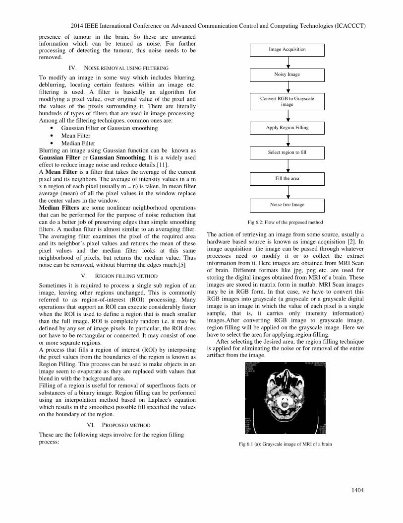
V. EXPERIMENTAL RESULTS
A. Experimental Model Setup
This section describes the implementation of
the proposed k-means clustering algorithm and also
analyzes the results of the experiments. The proposed
algorithm is simulated with NS2 with the parameters
listed in Table 1. The simulation results have been
analyzed with four different performance metrics.
The experiment has been designed by varying the
total number of nodes and holding all other
parameters constant to compare with respect to the
different performance metrics. The results of the
proposed method, i.e. WMN with k-means clustering
approach, have been compared with the simple WMN
scenario, i.e. WMN without cluster.
G5
G3 G4
G2
G1
G5
G3 G4
G2
G1
Cluster 1 Cluster 2
518517
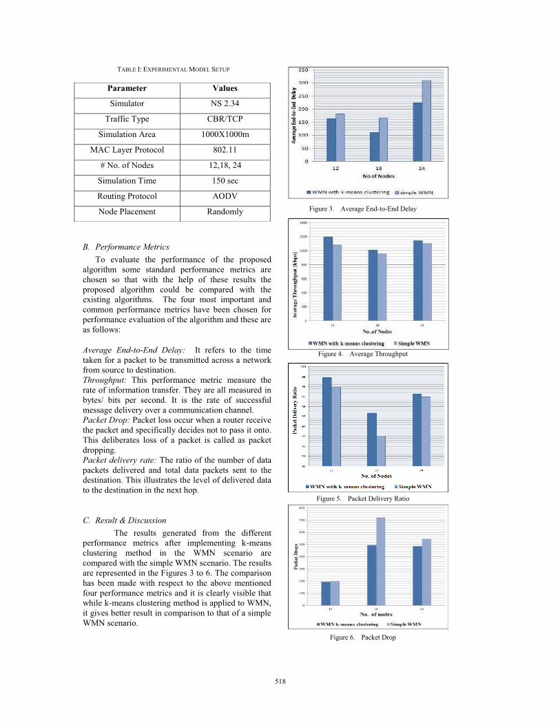
TABLE I: EXPERIMENTAL MODEL SETUP
B. Performance Metrics
To evaluate the performance of the proposed
algorithm some standard performance metrics are
chosen so that with the help of these results the
proposed algorithm could be compared with the
existing algorithms. The four most important and
common performance metrics have been chosen for
performance evaluation of the algorithm and these are
as follows:
Average End-to-End Delay: It refers to the time
taken for a packet to be transmitted across a network
from source to destination.
Throughput: This performance metric measure the
rate of information transfer. They are all measured in
bytes/ bits per second. It is the rate of successful
message delivery over a communication channel.
Packet Drop: Packet loss occur when a router receive
the packet and specifically decides not to pass it onto.
This deliberates loss of a packet is called as packet
dropping.
Packet delivery rate: The ratio of the number of data
packets delivered and total data packets sent to the
destination. This illustrates the level of delivered data
to the destination in the next hop.
C. Result & Discussion
The results generated from the different
performance metrics after implementing k-means
clustering method in the WMN scenario are
compared with the simple WMN scenario. The results
are represented in the Figures 3 to 6. The comparison
has been made with respect to the above mentioned
four performance metrics and it is clearly visible that
while k-means clustering method is applied to WMN,
it gives better result in comparison to that of a simple
WMN scenario.
Figure 3. Average End-to-End Delay
Figure 4. Average Throughput
Figure 5. Packet Delivery Ratio
Figure 6. Packet Drop
Parameter Values
Simulator NS 2.34
Traffic Type CBR/TCP
Simulation Area 1000X1000m
MAC Layer Protocol 802.11
# No. of Nodes 12,18, 24
Simulation Time 150 sec
Routing Protocol AODV
Node Placement Randomly
519518

VI. CONCLUSION
The internet gateways play an important role
in WMNs. And the limited capacity of the gateway
forbids it from handling a large amount of traffic and
making load balancing a crucial factor to improve the
network performance. A new approach to reduce the
overall workload of the gateways by distributing the
overall workload into a number of clusters throughout
the whole network is proposed based on the k-means
clustering approach to do the job of load balancing.
The simulation results confirm that by introducing the
k-means clustering approach the performance of
WMNs has increased in different aspects.
REFERENCES
[1] I. F. Akyildiz, X. Wang, “A survey on wireless mesh
networks,” IEEE Radio Communications, pp. S23-
S30, September 2005.
[2] I. F. Akyildiz, X. Wang, W. Wang, “Wireless mesh
networks: a survey,” Computer Networks, Science
Direct, Elsevier, pp. 445-487, June 2005.
[3] Abhishek Majumder, Sudipta Roy, Kishore Kumar
Dhar, “Design and Analysis of an Adaptive Mobility
Management Scheme for Handling Internet Traffic in
Wireless Mesh Network”, International Conference on
Microelectronics, Communication and Renewable
Energy (ICMiCR 2013), pp. 1-6, June, 2013.
[4] Yan Zhang, Jijun Luo, Honglin Hu, "Wireless mesh
network. architecture, protocols and standards,”
Auerbach Publications, 2007.
[5] Banani Das, Sudipta Roy, “Load balancing techniques
for wireless mesh networks: a survey,” IEEE
International Symposium on Computational and
Business Intelligence (ISCBI 2013), pp. 247-253,
August 24-26, 2013, New Delhi, India.
[6] Sudip Misra, Subhas Chandra Misra, Isaac Woungang,
“Guide to wireless mesh networks,” Springer-Verlag
London Limited, 2009.
[7] Yan Zhang, Jijun Luo, Honglin Hu, "Wireless Mesh
Network. Architecture, Protocols and Standards”,
Auerbach Publications, 2007.
[8] Tomas Johansson and Lenka Carr-Motyˇckov´, "On
Clustering in Ad Hoc Networks," Division of
Computer Science and Networking Lulea University
of Technology, August 17, 2003.
[9] Feng Zeng and Zhigang Chen, “Load Balancing
placements of gateways in Wireless mesh networks
with QoS constraints”, Young Computer Scientists.
2002. ICYCS 2008. The 9th International Conference
for IEEE, 2008.
[10] Waharte, Sonia, Raouf Boutaba, and Pascal Anelli,
“Impact of Gateways Placement on Clustering
Algorithms in Wireless Mesh Networks”, ICC.2001.
[11] Mohammad Shahverdy, Misagh Behnami, Mohmood
Fathy, “A new paradigm for load balancing in
WMNs,” in International Journal of Computer
Networks (IJCN), 3(4), pp.239-224, 2011.
[12] D. Chakraborty, M. K. Debbarma and Sudipta Roy,
“QoS Provisioning in WMNs: Challenges and a
Comparative Study of Efficient Methodologies”,
International Journal of Computer Application (IJCA),
65(3), pp.24-27, March 2013.
520519
A Tree Based Mobility Management Scheme for
Wireless Mesh Network
Abhishek Majumder1, Sudipta Roy2
1Department of Computer Science & Engineering Tripura University, Suryamaninagar
2Department of Information Technology Assam University, Silchar
Abstract- The importance of wireless mesh network is increasing
day by day with the popularity of hand held devices. But like other
wireless networks, one major problem of wireless mesh network is
maintenance of network connectivity to the mobile nodes in-spite-
of their random movement. For solving this problem, several
mobility management schemes such as Infrastructure-mode
Wireless Mesh Network (iMesh), MEsh networks with MObility
management (MEMO), Wireless mesh Mobility Management
(WMM) and Mesh Mobility Management (M3) have been
proposed. But the difficulty with these existing schemes is their
high communication cost. In this paper a tree based proactive
mobility management scheme has been proposed for handling both
internet and intranet traffic. A numerical analysis of the proposed
scheme has been carried out. Finally, the scheme has been
compared with iMesh, MEMO and WMM.
Keywords: Wireless Mesh Network, Mobility Management,
Handoff, Mesh Client, Mesh Router.
I. INTRODUCTION
Wireless Mesh Network (WMN) [1], [2] has a huge potential
to be the future technology for providing internet connections to
hand held devices. WMN has three types of nodes: mesh router
(MR), mesh client (MC) and gateway (GW). MCs are the users
of the WMN. Routing of packets from source MC to destination
MC is performed by the MR. The GW receives and transmits
the internet packets to and from the WMN.
WMN offer the advantages of self organizing and self healing
but it has the problem of providing seamless mobility. Many
mobility management schemes have been proposed. These
schemes are categorized into two types: tunnel based approach
and non-tunnel based approach. In tunnel based approach,
packets from the GW to MC will be sent through a tunnel but in
case of non-tunnel based approach no tunnel is used for sending
of packets. Mesh mobility management (M3) [3] is an example
of tunnel based approach. On the other hand, MEsh networks
with MObility management (MEMO) [4], infrastructure-mode
Wireless Mesh Network (iMesh) [5] and Wireless mesh
Mobility Management (WMM) [6] are the examples of non-
tunnel based approach. The advantage of non-tunnel based
scheme over tunnel based scheme is that it does not have any
tunnelling cost. But, it has the problem of heavy routing
overhead. In this paper, a non-tunnel based mobility
management scheme FPBR [7] has been enhanced to handle
both internet and intranet traffic.
The rest of the paper is organised as follows. Section II
presents a discussion on some of the mobility management
schemes. The proposed scheme has been discussed in section
III. System model and assumptions are presented in section IV.
The proposed scheme has been analyzed and compared in
section V and section VI respectively. Finally, the paper has
been concluded in section VII.
II. RELATED WORK
For solving the problem of mobility management, many non
tunnel based mobility management schemes have been
proposed. In this section some of those such as iMesh, MEMO
and WMM has been discussed.
In iMesh [4], when the MC moves out of the vicinity of a MC
and enters into the other, it broadcasts route update message in
the entire network using OLSR routing protocol.
In MEMO [5], as the MC move from old MR to new MR, the
old MR broadcasts a route error message in the entire network.
On receiving the route error message, all the MRs delete the
entry of the MC from its routing table. The MC then sends a
route reply message to the GW preemptively. If any
corresponding MC wants further communication with the MC,
it broadcasts route request message in the entire network. In
response, the corresponding MC sends back route reply
message. The same operation will be performed if the MC
needs to communicate with other MCs.
In WMM [6], each MR maintains a proxy table along with
the routing table. The proxy table will be used to store the mesh
router information of the MC. No separate route update
message is used in this scheme. Instead of that each data packet
carries the information of host MR of source MC. Intermediate
MR uses this information to update the host MR of the source
MC in the proxy table.
The problem of using MEMO and iMesh is that they have
high routing overhead. On the other hand, though WMM does
not have high routing overhead but it suffers from high packet
delivery cost due to the use of forward chain.
978-1-4799-6986-9/14/$31.00©2014 IEEE

III. PROPOSED SCHEME
In this section, the enhanced FPBR scheme has been presented.
The scheme uses a tree based approach and gateway (GW)
initiates the process to form the tree. This tree structure of the
MCs is used for mobility management of MCs. The scheme has
three parts:
A. Tree formation
The GW periodically broadcasts GW advertisement in the
entire network. The advertisement contains the level
information. Initially, the level is set to 0 by the GW. On
receiving the GW advertisement, each MR increments the value
of the level by 1, stores the level information and rebroadcasts
this message to its neighbour only once. This rebroadcasting
process continues till minimum distanced path is formed from
every MR to the GW. Thus, the GW acts as root of the tree and
each MR has three types of relationship with its neighbours:
child, parent and sibling. This information is maintained in
neighbour table of the MRs. There are mainly two objectives to
form the tree: minimization of hop count between GW and MRs
of the network and setting up of relationship between the MRs.
The relationships between the MRs are set up to categorize the
handoff of the MCs. Since, most of the traffic to and from the
MC belongs to the internet; the tree is formed to reduce the
packet delivery cost of internet packets thus reducing the
communication cost of the MCs.
B. Mobility Management
After the completion of link layer handoff, network layer
handoff will start. When the MC moves from one MR to
another, the MC sends route update message to the new MR. On
receiving the route update message, the new MR checks its
relationship with old MR. Based on the relationship, it performs
one of the following actions:
• If the new MR is the child of old MR, the new MR
forwards the route update message to the old MR. The old
MR sets the new MR as the next hop corresponding to the
MC in its routing table. The old MR will not forward the
route update message.
• If the new MR is the sibling of old MR, the new MR
broadcasts the route update message in the entire network
using OLSR [8] routing protocol. The GW and all the MRs
of WMN will update the routing table entry corresponding
to the MCs. Thus the forward pointer towards the MC is
reset.
• If the new MR is the parent of old MR, the new MR
first forwards route update message to its siblings. If the
sibling has entry of the MC in its routing table it will send
back an ACK message to the new MC and a forward
pointer is added from old MR to new MR. Otherwise, a
NACK message will be sent to the new MR. On receiving
the NACK message from all its siblings the MR broadcasts
the route update message to all the MRs of WMN using
OLSR and the forward pointer towards the MC gets reset.
C. Routing
There are mainly two types of traffic: internet and intranet.
Unlike FPBR [7] which is capable of handling only internet
traffic, the enhanced FPBR scheme can handle both internet and
intranet traffic.
Since the enhanced FPBR scheme uses a proactive routing
scheme, the GW and all the MRs of the WMN maintain a route
to every MC. When the GW receives an internet packet destined
to the MC it forwards the packet to the next hop towards the
destination. The intermediate MRs will also follow the process.
On receiving the packet the serving MR of the MC checks the
entry corresponding to the destination MC in its routing table. If
the MC is present in its vicinity the packet will be forwarded to
the MC. Otherwise, the packet will be forwarded to the current
MR of the MC through the forward chain.
Because of periodic gateway advertisement, each MC has a
route to the GW. Therefore, the uplink internet packets of the
MC will be directly sent from the current MC to the GW.
The MC sends upstream intranet packets to its current MR.
MR then routes the packets to the serving MR of the destination
MC. In case downlink intranet traffic, packets are received by
the serving MR of the MC. The serving MR forwards those
packets directly to the destination MC if the MC is within the
vicinity of the MR. Otherwise, the packets are forwarded to the
current MR of the MC and subsequently the current MR
forwards those packets to the MC.
IV. SYSTEM MODEL AND ASSUMPTIONS
In this section, the system model assumptions have been
presented. Without loss of generality, it can be assumed that
MC residence time in a MR follows exponential distribution
with rate λs [9] and session arrival rate and session departure
rate follows poission distribution with rate λa and λd
respectively [10]. Therefore, mobility of the MC follows
poission distribution with rate λs [11]. Let, average number of
neighbours, parents and children of a MR in the topology tree
be n, p and c respectively. The parameters used for analysis of
the proposed scheme and comparison with other existing
schemes are shown in table I.
TABLE I PARAMETERS AND THEIR INTERPRETATIONS
Parameter Interpretation
M Number of MRs in the WMN
α Average hop count between an arbitrary MR and the GW
く Average hop count between two arbitrary MRs
け Per hop communication latency
h Number of levels in the WMN
Ml Average number of MRs in each level
pr Average probability that the MR rebroadcasts the route request message in its neighbourhood
λp Average number of packets in a session per time unit
Ia Probability that the arriving session to MC be an internet session
Id Probability that the departing session from MC be an internet session
pNACK Probability that MR receives only NACK from its
siblings
Nactive Average number of corresponding MCs in the WMN per MC
rinter Percentage of downstream packets per internet session
rintra Percentage of downstream packets per intranet session
pg In WMM probability that current MR of MC does not know the location information of destination MC
Pq Probability that location query procedure is executed in WMM scheme
cmove Average displacement of the MC per MR association with respect to serving MR[12 ]
V. NUMERICAL ANALYSIS AND COMPARISON
In this section, the proposed scheme has been analysed and
compared with iMesh, MEMO and WMM. The comparison has
been carried out considering handoff cost/time unit, packet
delivery cost/time unit, query cost/time unit and total
communication cost/time unit.
A. Handoff Cost
As described in the previous section, handoff of a MC is
classified into three categories: sibling to sibling, parent to child
and child to parent. When the new MR is the sibling of the old
MR, the new MR broadcasts the route update message in the
entire network using OLSR protocol. Therefore, in this case the
handoff cost is ChstosFPBR = pr × M (1)
When the new MR is the child of the old MR route update
message will be forwarded to the old MR only. So, in this case
handoff cost is
ChstosFPBR = け (2)
When the new MR is the parent of old MR, new MR sends
route update message to sibling MRs. In response, if the new
MR receives only negative acknowledge (NACK) from all
neighbouring MRs, the new MR will send a location update
message in the entire network. Here handoff cost is the
summation of the cost incurred by message transfer between old
and new MR and broadcasting of route update message.
Therefore, the cost is, (2×け + pr×M). On the other hand, if the
new MR receives an acknowledge (ACK) from any neighbour
MR the cost for handoff will be 2×け.Therefore, in case of parent
to child movement the handoff cost is,
ChctopFPBR = 2×け + pNACK×pr×M (3)
Since the handoff takes place when MC moves into the
vicinity of new MR, handoff cost per time unit of the proposed
scheme is,
ChFPBR = {ChstosFPBR × (n-c-p)/n + ChctopFPBR × c/n+ChctopFPBR ×
p/n}×λs×cmove (4)
In [11] the handoff cost of WMM has been calculated as,
ChWMM = 2× け ×λs (5)
As presented in [11] the handoff cost per time unit of MEMO
is,
ChMEMO = {M+α×け+Nactive×(M+く×け)}×λs (6)
In case of iMesh, every handoff triggers broadcast of route
update messages in the entire network using OLSR. Therefore,
handoff cost per time unit is,
Chimesh = λs× pr × m (7)
B. Packet Delivery Cost
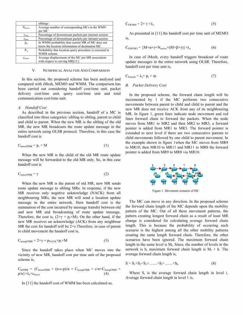
In the proposed scheme, the forward chain length will be
incremented by 1 if the MC performs two consecutive
movements between parent to child and child to parent and the
new MR does not receive ACK from any of its neighbouring
MR. In figure 1, green lines indicate node movement and red
lines forward chain to forward the packets. When the node
moves from MR1 to MR2 and then MR2 to MR3, a forward
pointer is added from MR1 to MR3. The forward pointer is
extended to next level if there are two consecutive parents to
child movements followed by one child to parent movement. In
the example shown in figure 1when the MC moves from MR9
to MR10, then MR10 to MR11 and MR11 to MR8 the forward
pointer is added from MR9 to MR8 via MR10.
The MC can move in any direction. In the proposed scheme
the forward chain length of the MC depends upon the mobility
pattern of the MC. Out of all these movement patterns, the
pattern creating longest forward chain as a result of least MR
change is considered for calculating average forward chain
length. This is because the probability of occurring such
scenario is the highest among all the other mobility patterns
creating the same length forward chain. Therefore, the other
scenarios have been ignored. The maximum forward chain
length in the same level is Ml. Since, the number of levels in the
network is h, maximum forward chain length is Ml × h. The
average forward chain length is,
S = S1+S2+S3+……+Si+……+Sh (8)
Where Si is the average forward chain length in level i.
Average forward chain length in level 1 is,
Figure 1. Movement scenario of MC
S1 = 1×((p-1)/n) ×(c/n) ×(1-pNACK)+2×((p-1)/n)2 ×(c/n) ×((c-1)/n) × (1-pNACK)2+3×((p-1)/n)3 ×(c/n) ×((c-1)/n)2 × (1-pNACK)3+…….+ Ml×((p-1)/n)Ml ×(c/n)×((c-1)/n)(Ml-1)×(1-pNACK)Ml
( )( )( )
( ) ( ) ( )
( )( )( )
( ) ( ) ( )
( )( )( ) ⎥⎥⎥⎥⎥
⎦
⎤
⎢⎢⎢⎢⎢
⎣
⎡
−−−
−
−−−
−
−−−
−
−−−
−
−−
=
NACKp
n
p
n
c
lM
NACKp
lM
n
plM
n
cl
M
NACKp
n
p
n
c
lM
NACKp
lM
n
plM
n
c
NACKp
n
c
n
p
111
1
111
21
111
111
1
11 (9)
If the forward chain is extended to level 2, the forward chain
length in level 2 is,
S2 = (Ml+1)×((p-1)/n)(Ml+1) ×(c/n)2×((c-1)/n) Ml ×(1-pNACK)Ml+1+(Ml+2)×((p-1)/n)(Ml+2) ×(c/n)2×((c-1)/n) Ml+1×(1-pNACK)Ml+1+…..+2×Ml×((p-1)/n)2Ml×((c-1)/n) 2Ml-1×(c/n)2×(1-
pNACK)2Ml
( ) ( ) ( ) ( )
( )( )( )
( ) ( ) ( ){ }( ) ( ) ( )
( ) ( ) ( )
( )( )( ) ⎥⎥⎥⎥⎥⎥
⎦
⎤
⎢⎢⎢⎢⎢⎢
⎣
⎡
−−−
−
−−−
−+
−−−
×−
−−−
−×
×−
−−−
×
+−×
−××
+−=
NACKp
n
c
n
p
lM
NACKp
lM
n
clM
n
p
lM
NACKp
lM
n
clM
n
pl
M
lM
NACKp
lM
n
clM
n
pl
M
NACKp
n
c
n
p
Ml
NACKp
Ml
n
c
n
cMl
n
p
111
1
111
1
111
111
1
111
1
1
11
1211
(10)
For 2 ≤ i ≤ h if the forward chain is extended to level i, the
forward chain length in level i is,
( )( ) ( ) ( )( )
( )( )
( )( )( )
( ) ( ) ( ) ( ){ }( ) ( ) ( )
( ) ( ) ( )
( )( )( ) ⎥⎥⎥⎥⎥⎥
⎦
⎤
⎢⎢⎢⎢⎢⎢
⎣
⎡
−−−
−
−−−
−+
−−−
×−
−−−
−××−
×
−−−
−×
+−−×
−+−−××
−+−−=
NACKp
n
c
n
p
lM
NACKp
lM
n
clM
n
p
lM
NACKp
lM
n
plM
n
cl
M
lM
NACKp
lM
n
clM
n
pl
Mi
NACKp
n
c
n
pl
Mi
NACKp
il
Mi
n
ci
n
cil
Mi
n
piS
111
1
111
1
111
111
11
111
1
1111
211111
(11)
The serving MR of the MC receives the downstream internet
packets from the GW and forwards those to the current MR. Per
packet delivery cost of downstream internet packet is,
CpinterdFPBR = け×(α+S) (12)
The upstream internet packets are directly sent by the current
MR of the GW. Therefore, per packet delivery cost of upstream
internet packet is,
CpinteruFPBR = け×α (13)
The upstream intranet packets are directly sent from the
current MR to the serving MR of corresponding MC. The
serving MR then forwards those packets to the current MR of
the MC. Therefore, per packet delivery cost of upstream intranet
packet is,
CpintrauFPBR = け×(く+S) (14)
Like upstream intranet packets the downstream intranet
packets will also incur the same packet delivery cost because
the routing process of both of them is similar. So,
CpintradFPBR = け×(く+S) (15)
For calculating packet delivery cost per time unit both
internet and intranet packets are considered. In case of intranet
packets, upstream intranet packets from a MC are also
downstream intranet packets for other MCs. Therefore, to
calculate intranet packet delivery cost per time unit only
downstream intranet packets have been considered. Packet
delivery cost per time unit is,
CpFPBR = {CpinterdFPBR×100
int err
+ CpinteruFPBR× ( )100
int1 err
− } ×(λa×Ia+
λd×Id) ×λp+ CpintradFPBR×{ λa×(1-Ia) ×int
100
rra + λd×(1-Id) ×
int
100
rra }×
λp (16)
In case of WMM average forward chain length for
downstream internet packets is [11],
FCgmWMM
=( ) ( ) ( ){ }( ) ( ) ( ){ }
1
100
int11100
int1
100
int11100
int1
−
⎥⎥⎦⎤
⎢⎢⎣⎡
−××−+−××+
−××−+−××
××ra
r
gp
dIer
r
dI
pd
rar
gp
aIer
r
aI
pa
movecsλλ
λλλ (17)
Per packet delivery cost of downstream internet packet is
[11],
CpinterdWMM = (α+ FCgmWMM)×け (18)
Per upstream internet packet delivery cost is [11],
CpinteruWMM = α× け (19)
Delivery cost of a downstream intranet packet routed through
the GW to the MC is [11],
CpintragdWMM = (2×α+ FCgmWMM)×け (20)

Average forward chain length for the downstream intranet
packets that are directly routed from the corresponding MC to
the receiving MC is [11],
FCintraWMM =( ) ( )( ) ( )
1
100
int11
100
int11
−
−×−××+
−×−××
×× ⎪⎭⎪⎬⎫⎪⎩
⎪⎨⎧ra
r
dI
pd
rar
aI
pa
activeNmovecsλλ
λλλ
(21)
Per packet delivery cost of downstream intranet packets from
corresponding MC is [11],
CpintradWMM = (く+FCintraWMM) ×け (22)
Considering only downstream intranet packets, packet
delivery cost per time unit is,
CpWMM = {CpinterdWMM×rinter+ CpinteruWMM×(1-rinter)}
×λp×{λd×Id+λa×Ia}+{( CpintragdWMM×pg+ CpintradWMM×(1-pg)}×λp×rintra×{λa×(1-Ia)+ λd×(1-Id)} (23)
In case of MEMO per packet delivery cost of downstream
and upstream internet packets is [11],
CpinterdMEMO = CpinteruMEMO = α×け (24)
The intranet packet delivery cost is calculated as,
CpintraMEMO = く×け (25)
Therefore, considering only the downstream packets in case
of intranet traffic, packet delivery cost per time unit can be
calculated as,
CpMEMO = CpinterdMEMO× λp× λa×Ia×100
int err
+ CpinteruMEMO× λp×
λa×Ia× ( )100
int1
err
− + CpinterdMEMO× λp× λd×Id×100
int err
+ CpinteruMEMO×
λp× λd×Id× ( )100
int1
err
− + CpintraMEMO× λp × int
100
rra × {λa×(1-Ia)+
λd×(1-Id)} (26)
In iMesh downstream internet packets are directly sent from
the GW to the host MR. The host MR then forwards the packets
to the MC. So, downstream intranet packet delivery cost is,
Cpinterdimesh = α×け (27)
The upstream internet packets will also be directly sent from
the host MR to the GW. Therefore upstream internet packet
delivery cost is,
Cpinteruimesh = α×け (28)
The host MR of the MC directly sends the upstream intranet
packets to the MR of corresponding MC. The same process will
be followed when the corresponding MC sends intranet packets
to the MC. Therefore, packet delivery cost of upstream and
downstream intranet packet is,
Cpintradimesh = Cpintrauimesh = く×け (29)
Internet as well as intranet packets are considered for
calculating packet delivery cost per time unit. In case of intranet
packets only downstream packets have been taken under
consideration. Therefore, packet delivery cost per time unit is,
CpiMesh = Cpinterdimesh× λp× λa×Ia×100
int err
+ Cpinteruimesh× λp×
λa×Ia× ( )100
int1
err
− + Cpinterdimesh× λp× λd×Id×100
int err
+ Cpinteruimesh× λp×
λd×Id× ( )100
int1
err
− + Cpintradimesh× λp ×int
100
rra × {λa×(1-Ia)+ λd×(1-Id)}
(30)
C. Query Cost
The enhanced FPBR scheme uses proactive strategy for
routing of packets. Each MR maintains a route to the serving
MR of the MC. Therefore, no query message will be sent in this
scheme.
In WMM the GW broadcasts route request message in the
entire network only when the MC wakes up from sleep mode or
the GW initiates the first internet session to the MC. Therefore,
query cost per time unit is [11],
CqWMM = (pr×M+く×け) × Pq× ( )sw
sw
ωω
ωω
+
× (31)
Where ωw and ωs are switching rates from sleep mode to
active and from active mode to sleep mode respectively.
In MEMO before initializing an intranet session if the host
MR of the source MC does not have route to destination MC, it
broadcasts a route request message in the entire network. Cost
for broadcasting the message is, M. The host MR of destination
MC sends back route reply message and cost for that is く×け. Therefore, query cost per time unit,
CqMEMO = (M+ く×け) ×(1-Id) ×λd×pg (32)
In iMesh each MR maintains a route to all the MCs of the
network. So, this scheme will not have any query cost.
D. Total Communication Cost
Total communication cost per time of the enhanced FPBR
scheme, WMM, MEMO and iMesh is,
TCFPBR= ChFPBR+ CpFPBR (33)
TCWMM= ChWMM+ CpWMM+ CqWMM (34)
TCMEMO= ChMEMO+ CpMEMO+ CqMEMO (35)

TCiMesh= Chimesh+ CpiMesh (36)
VI. PERFORMANCE ANALYSIS
This section presents a performance comparison of the
enhanced FPBR scheme with WMM, MEMO and iMesh. The
parameters used for comparison are: handoff, packet delivery
cost and total communication cost per time unit. For
comparison with respect to any parameter the following metric
is used [11],
F% = 100×− ⎟⎠
⎞⎜⎝⎛
FPBRC
FPBRC
otherC
(37)
If CFPBR > Cother, the cost of FPBR is F% higher than that of
the other scheme. Otherwise, the cost of FPBR is F% less than
other scheme. Typical values of parameters are shown in table
II. TABLE II
TYPICAL VALUES OF PARAMETERS
Parameter Value
M 1000
] 50
〈 30
Γ 0.1
N 6
P 2
Ml 20
h 50
pr 0.4
λp 1000
rinter 0.8
rintra 0.5
Ia 0.8
Id 0.7
pNACK 0.1
Nactive 30
Fig. 2 shows a comparison of handoff cost/sec of FPBR,
WMM, iMesh and MEMO. In this case, the value of λs and λd is
set to 0.5. The handoff cost of MEMO is the highest because in
this scheme after every handoff the old MR broadcasts route
error message, the new MC sends a proactive route reply
message to the GW and the corresponding MCs initiates a route
discovery process to the MC. Handoff cost of iMesh is higher
than that of FPBR and WMM. This is because after every
handoff the host MC broadcasts a route update message using
OLSR routing protocol. On the other hand, in FPBR route
update message is broadcasted using OLSR only when the
conditions discussed in section III are satisfied. Therefore,
FPBR incurs handoff cost less than that of MEMO and iMesh.
WMM has the lowest handoff cost since no separate route
update message is used in this scheme and only forward pointer
is added from old MR to the new MR.
Fig. 3 shows the variation of packet delivery cost/sec with the
increase in λa. WMM has the highest packet delivery cost
because the scheme uses forward pointer to forward packets
from old MR to new MR till the sender MR or GW has updated
route information. Packet delivery cost of FPBR is much less
than that of WMM because forward pointer is added only when
the conditions discussed in subsection B of section V are
satisfied. MEMO and M3 has the lowest packet delivery cost
because the schemes do not use any forward pointer. With the
increase in λa number of downstream packets increases.
Therefore, packet delivery cost of all the schemes also
increases.
Figure 4 shows the change in total communication cost/sec of
MEMO, WMM, iMesh and FPBR. MEMO has the highest total
communication cost because of its high handoff cost and query
cost. The total communication cost of WMM is higher than that
of iMesh and FPBR. This is because of its high packet delivery
cost and query cost. iMesh has higher total communication cost
than FPBR because of its high handoff cost. FPBR incurs low
handoff cost and packet delivery cost. Therefore, it has the
lowest packet delivery cost. FPBR incurs 379.71%, 2.07% and
7.59% less total communication cost/sec compared to MEMO,
iMesh and WMM respectively.
Figure 3. Effect of λa on Packet delivery cost
Figure 2. Effect of λa on Handoff cost

Handoff cost/sec, packet delivery cost/sec and total
communication cost/sec of MEMO, iMesh, FPBR and WMM
are shown in figure 5, figure 6 and figure 7 respectively. The
value of both λa and λs is set to 0.5. As λd increases handoff
cost/sec, packet delivery cost/sec and total communication
cost/sec of all the four schemes also follow the same behaviour
as shown in figure 2, figure 3 and figure 4 respectively. The
reasons for this are also similar. The total communication cost
of FPBR is 373.94%, 2.58% and 8.01% less than that of
MEMO, iMesh and WMM respectively.
Figure 8 shows the variation of handoff cost/sec as λs
increases. Here λa = 0.5 and λd = 0.5. With the increase in λs
handoff cost of MEMO increases at a higher rate compared to
the rest three schemes. This is because increase in λs increases
number of handoff/sec of a MC. Moreover, per handoff cost in
case of MEMO is also high. The handoff cost of iMesh
increases at a much lower rate compared to MEMO. But the
rate is higher than that of FPBR and WMM. This is because
after every handoff the MC broadcasts a route update message
using OLSR. The increase rate of handoff cost of FPBR is less
than that of iMesh since in this scheme the MC broadcasts route
update message only in limited occasion. WMM does not use
any route update message. Therefore, its handoff cost does not
change with increase in λs.
Figure 9 shows effect of λs on packet delivery cost/sec. As λs
increases the packet delivery cost of MEMO and iMesh remains
unchanged because the packets are directly sent from the source
MR to the host MC. In case of WMM forward chain length
increases as the value of λs increases. Therefore, packet delivery
cost of WMM also increases. The packet delivery cost FPBR
remains unaffected with increase in λs because the forward
chain length is only dependent upon mobility pattern. It does
not depend on mobility rate of the MC.
Figure 8. Effect of λs on Handoff cost
Figure 7. Effect of λd on Total communication cost
Figure 6. Effect of λd on Packet delivery cost
Figure 5. Effect of λd on Handoff cost
Figure 4. Effect of λa on Total communication cost

Variation in total communication cost/sec of MEMO, iMesh,
WMM and FPBR are shown in figure 10. The total
communication cost of MEMO increases at the highest rate
compared to rest of the schemes. The reason behind this is its
high handoff cost. WMM has higher total communication cost
compared to iMesh and FPBR because of its high packet
delivery cost and query cost. But the increase rate is less than
that of iMesh. The handoff cost of iMesh is high and it increases
at a higher rate compared to WMM. Therefore, the total
communication cost of iMesh is higher than that of FPBR but it
increases at a rate higher than both FPBR and iMesh. FPBR has
the lowest total communication cost compared to all the three
schemes. This is because of its low handoff cost and packet
delivery cost. Total communication cost of FPBR is 403.5%,
2.86% and 8.03% less than that of MEMO, iMesh and WMM
respectively.
VII. CONCLUSION
This paper proposes a mobility management protocol named
FPBR for handling both intranet and internet traffic. The
scheme has been analysed and compared with MEMO, iMesh
and WMM. Numerical analysis shows that FPBR performs
better than MEMO, iMesh and WMM with respect to handoff
cost, packet delivery cost and total communication cost.
REFERENCES
[1] I.F.Akyildiz and X. Wang, “A Survey on Wireless Mesh Networks”, IEEE Communications Magazine, vol. 43, no. 9, pp.S23 - S30.
[2] I. F. Akyildiz, X. Wang, and W. Wang, “Wireless mesh networks: a survey,” Computer Networks, vol. 47, no. 4, pp. 445–487, 2005.
[3] R. Huang, C. Zhang and Y. Fang, “A Mobility Management Scheme for Wireless Mesh Networks”, IEEE GLOBECOM, pp. 5092-5096, 2007.
[4] Ren M. et al., “MEMO: An Applied Wireless Mesh Network with Client Support and Mobility Management”, IEEE GLOBECOM, pp. 164-170, 2007.
[5] V.Navda, A.Kashyap and R.S.Das, “Design and Evaluation of iMesh: an Infrastructure-mode Wireless Mesh Network”, Sixth IEEE International Symposium on a World of Wireless Mobile and Multimedia Networks, pp. 164-170, 2005.
[6] D. Hwang, P. Lin and C. Gan, “Design and performance study for a mobility management mechanism (WMM) using location cache for wireless mesh networks,” IEEE Transaction on Mobile Computing, vol. 7, no. 5, pp. 546-556, 2008.
[7] A. Majumder, S. Roy, “A Forward Pointer Based Mobility Management Scheme for Multi-Hop Multi-Path Wireless Mesh Network”, ICDSE, pp. 194-197, 2012.
[8] T. Clausen and P. Jacquet. Optimized link state routing protocol (OLSR). RFC 3626, October 2003.
[9] S. Pack, H. Jung, T. Kwon and Y. Choia, “SNC: a selective neighbor catching scheme for fast handoff in 802.11 wireless networks,” ACM SIGMOBILE Mobile Computing and Communication Reviews, vol. 9, no. 4, pp. 39-49, 2005.
[10] S. Kwon, S. Y. Nam, H. Y. Hwang, and D. K. Sung, “Analysis of a mobility management scheme considering battery power Conservation in IP-based mobile networks, ” IEEE Transactions on Vehicular Technology, vol. 53, no. 6, pp. 1882-1890, 2004.
[11] A. Majumder and S. Roy, “Design and Analysis of a Dynamic Mobility Management Scheme for Wireless Mesh Network,” The Scientific World Journal, vol. 2013, Article ID 656259, 16 pages, 2013. doi:10.1155/2013/656259.
[12] A. Majumder, S. Roy, and K. K. Dhar, “Design and analysis of an adaptive mobility management scheme for handling traffic in wireless mesh network,” International Conference on Microelectronics, Communications and Renewable Energy, pp. 1–6, 2013.
Figure 10. Effect of λs on Total communication cost
Figure 9. Effect of λs on Packet delivery cost

2015 Intenational Symposium on Advanced Computing and Communication (ISACC)
Automatic Brain Tumor Segmentation in MRI: Hybridized Multilevel Thresholding and Level Set
Malsawm Dawngliana Department of IT, Assam University,
Silchar, India [email protected]
Daizy Deb Department of IT, Assam University,
Silchar, India [email protected]
Abstract- Segmentation of tumor from magnetic resonance
image (MRI) brain images is an emergent research area in the
ield of medical image segmentation. As segmentation of brain
tumor plays an important role for necessary treatment and
planning of tumor surgery. However, segmentation of the brain
tumor is still a great challenge in clinics, specially automatic
segmentation. In this paper we proposed hybridized multilevel
thresholding and level set method for automatic segmentation of
brain tumor. The innovation for this paper is to interface the
initial segmentation from multilevel thresholding and extract a
ine portrait using level set method with morphological
operations. The results are compared with the existing method
and also with radiologist manual segmentation which conirm the
effectiveness of this hybridized paradigm for brain tumor
segmentation.
Kywords- Magnetic Resonance Imaging(MRI), Brain tumor,
nmltilevel thresholding, level set method, medical image processing.
I. INTRODUCTION
Brain is built up of numerous types of cells. These cells typically grow and divide in a self-restrained and formal manner to produce new cells. Worthlessly, new cells continue to produce which lead to a mass of extra tissue called brain tumor. Brain tumor can be benign (not cancerous) or malignant (cancerous), the cells of malignant tumors are abnormal and divide numerously, nearby cells will be attack and damage the healthy adjacent tissues.
Modem technology does not provide information about tumor observation and patten, judgment of lesion is still carried out manually. The main disadvantages of manual segmentation are: it is time consuming and fully rely on human decision. According to the population and the number of patients, manual judgment is bulky in everyday clinic and led to human errors. Therefore development of tools for automatic judgment of lesion is a demand in today's senario.
To overcome these problems, automatic brain tumor segmentation was proposed by Singh,P [ I] for initial segmentation, FCM algorithm is employed which cluster the MRI brain image, rom these clusters the desired cluster must be selected manually for automatic initialization. Hence one
978-1-4673-6708-0/15/$31.00 ©20 15 IEEE
Mousum Handique Department of IT, Assam University,
Silchar, India [email protected]
Sudipta Roy Department of IT, Assam University,
Silchar, India [email protected]
can say that it is not fully automatic as human intervention is involved. The selected cluster is taken as input for levelset method, which segment the tumor part without the need of reinitialization. If the initial segmentation is automated, it will give fully automatic segmentation method.
In medical image segmentation, classical thresholding plays an important role as it separate the object rom the background using simple intensity value variation, it separate the image into two groups according to threshold value [2]. Natarajan,P [3] employs classical thresholding operation with morphological operation for automatic brain tumor detection, in this approach, the threshold value must be adjusted manually depending upon the input image intensity. Classical thresholding is not effective for initial medical image segmentation due to the presence of uneven intensity variation in an image.
Multilevel thresholding using type-II uzzy sets was proposed by Ritambhar Burman [4]. This multilevel thresholding can segment an image into number of groups, which will make thresholding more robust for initial segmentation in medical images. Hence, a hybridized technique for fully automatic brain tumor segmentation is proposed in this paper which make use of multilevel thresholding based on image intensity for initial segmentation and level set method for refmement of tumor based on image boundary variation.
This paper is organized as follows. The background work is discussed in section II. The proposed method is discussed in section III which starts with a lowchart of the proposed technique. Experimental results and performance evaluation of our proposed method and existing method is illustrated In section IV, followed by the conclusions in section V.
II. BACKGROUND WORK
By using just a powerul magnetic ield and radio frequency pulses MI operates, which gives input to a computer which produce detailed image of organs, sot tissues and bones. Detailed MR images allow physicians to evaluate

various treatment and surgery can be plan by the use of brain MRI. Initially MRI images are stored in DICOM format, which can be urther pre-processed for higher image analysis.
The sample images are acquired rom BraTS database which is in DICOM format [5]. As the dataset contain skull, which is included in the image volume, it is prefer to remove this skull before the system process. Skull stripping is performed using Brain Extraction Tool (BET) [6] using this tool, the skull part is removed and only the brain is extracted. The output MRI slice is fed to the system which give advantages in speed and accuracy for higher image analysis.
III. PROPOSED METHOD
The lowchart shown in Fig. 1 ully illustrates the overall procedure of the system. Firstly, the system starts with an MRI brain image as an input. Here, pre-processing of the input image with the help of median ilter algorithm and histogram equalization. The produced image undergo Multilevel Thresholding method which partition the image into meaningul parts and morphological operation is to ilter out noises but preserve the important information. Finally, enhanced level set method for fme delineation of brain tumor takes place. The segmented tumor image is produced as an output.
A. Pre-processing In this phase, the input image is treated with initial
processing before it passes through any special purpose processing. Here the image improves the quality and noises are removed. As the brain tumor is going to be segmented rom the MRI brain image, it must have minimum noise with high image quality. It consists of two sub-steps:
1) Median Filtering: Median ilter is oten choose to perform noise reduction in
an image. Window slide entry by entry which is the main idea of median ilter, it slide over the whole image, the pixel at the centre is the central pixel. The neighboring pixels are ranked according to intensity and the median value replace the central pixel value Advantage of median ilters algorithm is that it can perform an excellent operation of rejecting certain types of noise, in particular impulse noise in which some individual pixels have extreme values [7]. Since the output pixel value is one of the neighboring values, new alien values are not created. Edges are preserves while removing noise; it is possible to apply repeatedly if necessary. This iltering algorithm enhances the quality of the MRI brain images.
2) Histogram Equalization: Histogram equalization makes use of image histogram for
contrast adjustment, so that the intensities can be distributed better. The input image may be composed of uneven distribution of intensity, which makes the image having weak contrast and low quality. The solution is to perform histogram equalization. It is applied for enhancing the appearance of an image.
Pre-processing
Median Filtering
Histogram Equalization
Segmentation
Multilevel Thresholding
Feature Extraction
Extracted Tumor
Fig. I Block diagram of proposed method
B. Multilevel Thresholding Ater the MRI brain images undergo pre-processing stage,
images are fed to Multilevel Thresholding stage. This Multilevel Thresholding method threshold an image by using uzzy membership values which partition the histogram of an image. Using Type-II uzzy sets, it obtain optimal image threshold by employing ultra fuziness [4]. The obtained results are hereby more justiiable for medical images.
A Type-II fuzzy set A in a uzzy inite set X={XI + X2 + ...... + Xn } may be represented as [8]:
Where, lu(x) and lL (X) are the upper and lower membership unction respectively which range rom ° to 1.
Let the input image 0 be of size M*N, with f(m,n) as the grey value. L is the number of grey values in which image I can be represented, the set of all grey levels {O, I,2 ... L- I} IS
represented as G.
f(m, n)EGf(m, n)EI Dk = {(m,n):f(m,n) = k,kE{O,1,2 ... ,L -I}} (2)

Let H={ho,hJ, ... hL_dbe the normalized histogram of the image where hk=nk/(M*N), nk is the number of pixels in Dk.
The ultra-uzziness for an image for the klh level is given by:
Where O<k<=N+ I, N is the number of threshold level. Here we consider N=3. I represent the grey levels.
1 Here we have used (luh = ((lU)k)a and (lLh
((ldk)U, considering a= l.5.
The thresholds for the image is that point, where the membership value of a level of segmentation falls to 0.5, DE is used to reduce the search time to ind the optimal thresholds.
Algorithm for Multilevel image thresholding based on type II uzzy sets:
1.
11.
Calculate the image histogram. Give the number of threshold level N.
III. Apply Differential Evolution to optimize the search space.
IV. Calculate the upper and lower membership unctions. v. Calculate the ultra uziness for each position.
vi. Obtain the membership values. vii. Get the optimal threshold image.
. Feature Extraction: Ater multilevel thresholding, the segmented image
undergo feature extraction stage where removal of noise is done without destroying the original properties and extract the feature. In this stage two methods are used: Morphological operation and Level Set method.
1) Morphological Operation: The term morphology discuss about image processing
technique which takes into consideration of the structure and shape of an objects. Binary images may contain numerous noise, hence it is used here as object reinement. It reines the noise present but still preserve the original properties of the object. It works on the principle of pre-deined rules in short time. It simply means to identiy the shape and structure of object within the image. It operates on the basis of pixel comparision with the neighbouring pixels. Morphological operation usually performed on binary images, the binary image have a pixel value of 0 or 1.
The advantage of morphological operations here is to ilter the object in multilevel thresholding due to noise but preserve the original image components. We observe that the noises are discrete and diverse. So at irst morphological operations should shrink and eliminate small pieces of objects in
Multilevel Thresholding segmentation, and then expand to recover the meaningful objects.
2) Levelset method: In this paper, we have used a level set evolution method
without re-initialization introduced by Li Chunming et aI., [9], which is based on energy penalty term to extract the brain tumor. Level set segment an image on the basis of pixels intensity and variational boundaries.
In the level set method, the evolution equation of the level set function 0 is given by:
d0 t + FIV01 = ° 0(O,x,y) = 0L(x,y) (4)
Where F is the extenal force which dependents on image information like image gradient and image intensity, this force F attracts the curves toward the edges. IV01 is the normal direction, 01 (x, y) is the initial contour.
The moving force F has to be stopped at the edge by an edge indication function g
1 (5)
Where G" is a Gaussian unction with the standard deviation ", * represents convolution, I is a given 2D image, V is the gradient operator, 1.1 is the modulus of smoothed image gradients.
Extenal energy function 01 (x, y) is deined as
(6)
Where v are constants and t > O.
The terms Lg(0) and ig (0) can be deined as
Lg(0) = In g"(0)IV0Idxdy (7)
ig (0) = In gH (-0)dxdy (8)
Where " is the univariate Dirac function, and H is the Heaviside unction.
The total energy unction is deined as
c (0) = tLgP(0) + cg,A.v(0) (9)
Here the total energy consist of internal energy term and extenal energy term. The intenal energy term P(0)penalizes the deviation of the level set unction rom signed distance unction and the extenal energy term cg•A,v(0) drives to

motion of the zero level set to the required image features like object boundaries.
The evolution equation of the level set unction is deined as: d0
= l [J - div (�)] + AS(0)div (g�) + vgS(0) (10) dt 1701 1101
The modiication of level set algorithm lead to fast image segmentation without the need of re-initialization.
IV. ESULT AND EVALUATION
We evaluate the performance of our proposed method and existing method by taking MRI brain dataset rom BraTS database [5] which was segmented by experts having different location, shape, size and contrast of tumor. The dataset is provided with ground truth, from which we can evaluate the segmentation accuracy. The same images are segmented with FCM-Levelset method [ I] and proposed MLT-Levelset method performance have been recorded and performance assessment table is shown in Table 1 and Figure 2.
Fig. 2 (a) Input MRI brain image. (b) Segmented tumor with FCM-Levelset algorithm. (c) Segmented tumor with ML TLevelset algorithm. (d) Ground truth segmented manually by the radiologist.
Table 1: Evaluation of the segmentation results for FCMLevelset method and MLT-Levelset method.
Volume metric functions for Volume metric functions for FCM-Levelset MLT-Levelset
S Ji S Ji 1 1.29 0.65 1.76 0.88 2 1.42 0.71 1.70 0.85 3 0.24 0.12 0.75 0.37 4 0.72 0.36 1.55 0.77 5 1.60 0.80 1.65 0.83
Average 1.05 0.53 1.48 0.74
The performance of these segmentation are validated by Dice similarity coeicient(S) [10] and Jaccard index [11]. Let a given image have pixels Ax and Bx belonging to class x in manual and in automatic segmentation respectively. IAxl imply the number of pixels in Ax. IBxl imply the number of pixels in Bx.
Dice similarity coeicient S is deined as:
s =
C121AxnBxll) IAxUBxl (11)
Dice value ranges rom [0,1], 0 for no similarity and 1 for ull similarity.
Jaccard index between two volumes is deined as,
Ji = IAxnBxl XIOO IAxUBxl (12)
Higher the value of S and Ji, and lower the value of FPVF, FNVF gives better segmentation result.
The performance assessment of our proposed method with the existing method [1] is shown in table 1 and igure 2. It shows that, the existing method gives l.05 out of 2 and 53% in similarity coeicient and Jaccard index while our proposed method gives 1.48 out of 2 and 74% respectively, which implies that our proposed method gives higher accuracy. This also implies that our proposed method have lower segmentation error and loss of expected tumor pixels are also greatly reduced.
v. CONCLUSION
Our proposed method deals with the hybridization of Multilevel Thresholding method and Levelset method. The Thresholding method segment the tumor region rom the brain image in a multiple level and Levelset without re-initialization technique is use to extract a ine portrait of the tumor area.

2
1.5
1
0.5
o FCM-Levelset
(Existing method)
• Dice Similarity (S)
MLT-Levelset (Proposed method)
• Jaccard index (Ji)
Fig. 3 Graphical representation of Dice similarity and Jaccard index for FCM-Level Set and proposed ML T-Level Set.
(Higher the value of S and Ji, gives better segmentation result. )
To summarize, we proposed a new hybridized technique for the segmentation of tumor rom MRI brain images. By comparing with the existing method and the ground truth provided, our proposed method demonstrate an impressive performance. However, in the uture work the shape deformation feature must be improve so as to get higher segmentation accuracy.
REFERENCES
[1] Singh, P.; Bhadauria, H.S.; Singh, A., "Automatic brain MRI image segmentation using FCM and LSM" Reliability, Infocom Technologies and Optimization (ICRITO) (Trends and Future Directions), 2014 3rd Intenational Conference, pp. l,6, 8-10 Oct. 2014.
[2] Gonzalez and R.C. Richard, Digital Image Processing, 2nd ed. India: Pearson Education, 2004.
[3] Natarajan, P.; Krishnan, N.; Kenkre, N.S.; Nancy, S.; Singh, B.P., "Tumor detection using threshold operation in MRI brain images," Computational Intelligence & Computing Research (ICCIC), 2012 IEEE Intenational Conference, pp. l ,4, 18-20 Dec. 2012.
[4] Burman,Ritambhar; Paul,Sujoy; Das,Swagatam,"A Differential Evolution Approach to Multi-level Image Thresholding Using Type II Fuzzy Sets," Swarm, Evolutionary, and Memetic Computing, 2013, 8297, 274-285, Springer International Publishing.
[5] www2.imm.dtu.dk/projectsIBRATS2012/ [6] S.M. Smith. Fast robust automated brain extraction.
Human Brain Mapping, 17(3):143-155, November 2002. [7] Jasdeep Kaur and Preetinder Kaur, "Fuzzy Logic based
Adaptive Noise Filter for Real Time Image Processing Applications", Intenational Jounal of Computer Applications 58(9): 1-5, November 2012.
[8] Jianhua Wu; Zhaoyu Pian; Li Guo; Kun Wang; Liqun Gao, "Medical Image Thresholding Algorithm Based on Fuzzy sets Theory," Industrial Electronics and Applications, 2007. ICIEA 2007. 2nd IEEE Conference, pp.919,924, 23-25 May 2007.
[9] Chunming Li; Chenyang Xu; Changfeng Gui; Fox, M.D., "Level set evolution without re-initialization: a new variational formulation," Computer Vision and Patten Recognition, 2005. CVPR 2005. IEEE Computer Society Conference, voLl, pp.430,436 vol. 1, 20-25 June 2005.
[10] D Shattuck, R Leahy, BrainSuite: an automated cortical surface identiication tool. Med. Imag. Anal. 6(2), 129-142 (2002).
[11] Jaccard, P., 1912. The distribution of lora in the alpine zone. New Phytologist 11, 37-50.

Identification of WBC based on Dynamic Clustering using Modified FCM Algorithm with an Approach to Optimal
Result Nur Alom Talukdar
Department of Computer Science and Engineering
Assam University Silchar, India
+91 3842 270988 [email protected]
Sudipta Roy Department of Computer Science and
Engineering Assam University
Silchar, India +91 3842 270990
ABSTRACT In medical diagnosis, analysis of the blood components is the most vital process. Among all the blood components, analysis of the White Blood Cell (WBC) is very crucial and important. Almost all types of deadly diseases including cancer are due to the abnormal presence of WBC. Proper identification of WBC is the only way for proper treatment. For the identification of WBC, in this paper, modified Fuzzy C-Means (FCM) clustering is used. In FCM, selection of the cluster is predefined and fixed based on assumption that degrades the quality of the result. It is unable to give the optimal result if the chosen cluster is wrong. In this paper, a dynamic clustering algorithm with a novel approach to produce the optimal result is proposed which can overcome these problems of classical FCM.
Keywords White Blood Cell; Dynamic Clustering; Optimal Result; Modified FCM; Cancer.
1. INTRODUCTION WBC has a great importance in medical diagnosis for proper treatment. WBC can be categorized into five different classes; namely neutrophils, basophils, eosinophils, lymphocytes and monocytes shown in Figure 1. Classes with “Phil” called granulocytes and indicate presence of granules. Classes with “cyte” called agranulocytes, indicates absence of granules [1].
From the study of related work and literature, it is observed that different researchers used different approach to implement FCM like, modified FCM [2], efficient FCM [3], penalized FCM [4] etc.
A method to segment image is proposed in [4] using a penalty term in FCM. The penalty term employed as a regulizer to penalize the object function of FCM. To implement this, the authors used neighborhood exception maximization approach and tried to reduce the sensitivity of FCM to noise.
Hung and Yang in [3] proposed a clustering approach to implement the FCM efficiently to reduce the computation time. For that they first recognized the centroid of the cluster from the original simplified set that accelerates the convergence time by refines the initial value of FCM.
Chinwarabhatet. al. address in [2] a work to segment WBC using modified FCM where they tried to minimize the iteration for clustering process. They used neighboring color pixel of its scattering as a reference. They considered the scattering size greater than a threshold value and then applied a thickening morphology.
In this paper, dynamic clustering approach is proposed for modified FCM algorithm for the optimal result.
(a) (b) (c)
(d) (e)
(f)
Figure 1. (a) Basophil; (b) neutrophil; (c) eosinophil (d) lymphocyte; (e) monocyte; (f) original blood image;
The rest of the paper is organized as below: Section 2 discusses about Clustering; Fuzzy C-Means is discussed in section 3; section 4 discusses the proposed Modified
Permission to make digital or hard copies of all or part of this work for personal or classroom use is granted without fee provided that copies are not made or distributed for profit or commercial advantage and that copies bear this notice and the full citation on the first page. Copyrights for components of this work owned by others than ACM must be honored. Abstracting with credit is permitted. To copy otherwise, or republish, to post on servers or to redistribute to lists, requires prior specific permission and/or a fee. Request permissions from [email protected]. ICCCT '15, September 25-27, 2015, Allahabad, India © 2015 ACM. ISBN 978-1-4503-3552-2/15/09 $15.00 DOI: http://dx.doi.org/10.1145/2818567.2824992

FCM. Section 5 discusses the proposed Dynamic Clustering approach using the Modified FCM. Experimental result is presented in section 6 and the work is concluded in section 7.
2. CLUSTERING Clustering is the process of sub-dividing a data set into
many parts with the homogeneity of the characteristics of data. It’s a state of art approach for segmentation. Clustering of data can be done by one of the two approaches namely Hard partition (crisp) and soft partition (fuzzy). In hard partition one point of data can belong to only one cluster i.e. membership of belongingness of the data is either 0 or 1 [5][6]. Whereas in fuzzy partition one data point can belong to more than one cluster i.e. membership of belongingness of the data is between 0 and 1.
3. FUZZY C-MEANS (FCM) FCM clustering is an approach of clustering data where
each datum may belong to more than one cluster. FCM works by assigning membership to each data point corresponding to each cluster center on the basis of distance between the cluster and the data point [7][8]. It is an iteration process, the partition matrix U is updated by Equation (1). ∪ij =
1
D ij D ik 2m−1
Ck =1
(1)
Which is followed by the update of the cluster centers Vjby Equation (2). 撃倹 =
戟件倹兼 .�件�件=1 戟件倹兼 �件=1
(2)
The algorithm is processed by minimizing Equation (3). 蛍兼 戟,撃 = .�件=1 戟件倹兼 経件倹2 系倹=1 (3)
Where,
X = {x1, x2, x3… xn} = the data,
C= cluster numbers in X,
m = fuzziness index, 1 ≤ m < ∞, U = fuzzy c-partition of X,
V = (v1, v2, v3… vc ) = vectors of centers,
Uij= the membership value of the ith datum for the jth cluster, Vj= (vj1, vj2, vj3… vjn)= center of cluster j,
Dij= Euclidean distance betweenith data andjth cluster center using proposed metrics [9].
The FCM algorithm is stated as below:
A. Algorithm FCM
1. Set cluster number (C), Fuzziness index (m), Maximum iteration (Imax).
2. Initialize matrix U(0) as U= [uij ] 3. For I =1,2,…, Imax , do:
a. Update the cluster centers using Equation (2) b. Update the membership matrices U(I) using Equation(1) c. Check U(I) with U(I+1) , if ||U(I+1)- U(I)|| < termination criteria, then stop;
Else Update U(I) =U(I+1).
4. MODIFIED FCM The FCM algorithm works by assigning membership to
each data point corresponding to each cluster center on the basis of distance between the cluster and the data point. It is an iterative process and in each iteration the cluster centers change their positions based on the distance between the data point and cluster center; distance calculation plays an important role in FCM. In modification of FCM, a new distance metric is proposed which outperforms the Euclidean metric. Experimental results are shown in the Figs. 4(a) and 4(b).
Considering the proposed metric; Equations (1), (2) and (3) can be rewritten as: ∪件倹=
1
�経 件倹 �経 件倦 2兼−1系倦=1
(4)
撃倹 = 戟件倹兼 .�件�件=1 戟件倹兼 �件=1
(5) 蛍兼 戟,撃 = .�件=1 戟件倹兼 ||�経件倹 ||2系倹=1 (6)
Where, PD is the proposed metrics and can be expressed as:
PD(x,v)= PD(v,x)= �件 − �件 2券件=1 , v and x are two points in the feature space.
5. DYNAMIC CLUSTERING APPROACH WITH MODIFIED FCM
In FCM, the selection of the cluster number is predefined, fixed and is based on assumption. It is very crucial to select the best cluster by only assumption. If the chosen cluster is wrong it degrades the quality of final result. This is a time consuming process also to select a cluster based on assumption and test the result and repeat the process for better result. In this paper a dynamic clustering approach is proposed. Instead of selecting the fixed cluster number a priory, here it is needed to select the minimum cluster to execute the clustering process. For the result optimization process, image quality measurement metric are used. The DCAMFCM algorithm is as below:
A. DCAMFCM Algorithm
1. Set minimum and maximum cluster number (Cmin and Cmax), Fuzziness index (m), Maximum iteration (Imax).
2. Initialize matrix U(0) as U= [uij ] 3. For C= 2,3,…,Cmax, do; 4. For I =1,2,…, Imax , do:
a. Update the cluster centers �件荊 using Equation (5) b. Update the membership matrices U(I) using
Equation(4) c. Check U(I)with U(I+1) ,
if || U(I+1)- U(I) || < termination criteria, then stop;
Else
Update U (I) =U (I+1).
5. Check for optimal result; if optimal, then stop;
Else
Increment C.
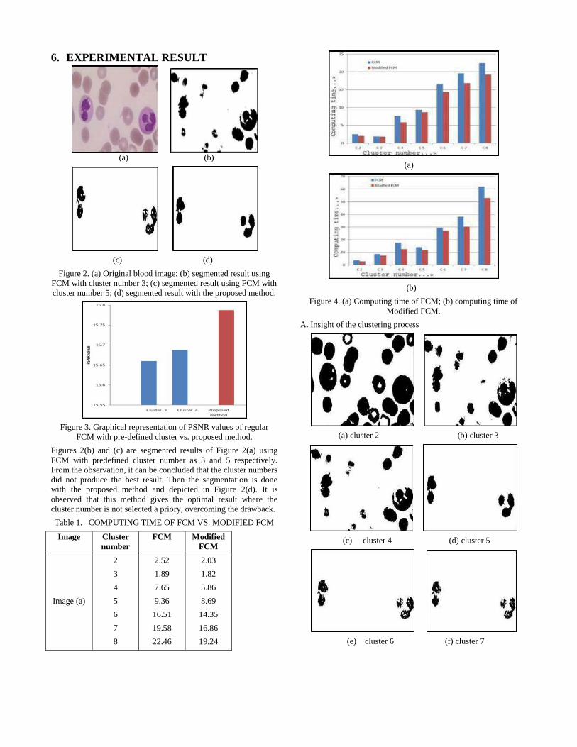
6. EXPERIMENTAL RESULT
(a) (b)
(c) (d)
Figure 2. (a) Original blood image; (b) segmented result using FCM with cluster number 3; (c) segmented result using FCM with cluster number 5; (d) segmented result with the proposed method.
Figure 3. Graphical representation of PSNR values of regular
FCM with pre-defined cluster vs. proposed method.
Figures 2(b) and (c) are segmented results of Figure 2(a) using FCM with predefined cluster number as 3 and 5 respectively. From the observation, it can be concluded that the cluster numbers did not produce the best result. Then the segmentation is done with the proposed method and depicted in Figure 2(d). It is observed that this method gives the optimal result where the cluster number is not selected a priory, overcoming the drawback.
Table 1. COMPUTING TIME OF FCM VS. MODIFIED FCM
Image Cluster number
FCM Modified FCM
Image (a)
2
3
4
5
6
7
8
2.52
1.89
7.65
9.36
16.51
19.58
22.46
2.03
1.82
5.86
8.69
14.35
16.86
19.24
(a)
(b)
Figure 4. (a) Computing time of FCM; (b) computing time of Modified FCM.
A. Insight of the clustering process
(a) cluster 2 (b) cluster 3
(c) cluster 4 (d) cluster 5
(e) cluster 6 (f) cluster 7
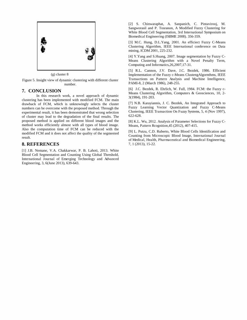
(g) cluster 8
Figure 5. Insight view of dynamic clustering with different cluster number.
7. CONCLUSION In this research work, a novel approach of dynamic
clustering has been implemented with modified FCM. The main drawback of FCM, which is unknowingly selects the cluster numbers can be overcome with the proposed method. Through the experimental result, it has been demonstrated that wrong selection of cluster may lead to the degradation of the final results. The proposed method is applied on different blood images and the method works efficiently almost with all types of blood image. Also the computation time of FCM can be reduced with the modified FCM and it does not affect the quality of the segmented result.
8. REFERENCES [1] J.B. Nemane, V.A. Chakkarwar, P. B. Lahoti, 2013. White Blood Cell Segmentation and Counting Using Global Threshold, International Journal of Emerging Technology and Advanced Engineering, 3, 6(June 2013), 639-643.
[2] S. Chinwaraphat, A. Sanpanich, C. Pintavirooj, M. Sangworasil and P. Tosranon, A Modified Fuzzy Clustering for White Blood Cell Segmentation, 3rd International Symposium on Biomedical Engineering (ISBME 2008). 356-359.
[3] M.C. Hung, D.L.Yang, 2001. An efficiect Fuzzy C-Means Clustering Algorithm, IEEE International conference on Data mining, ICDM 2001, 225-232.
[4] Y.Yang and S.Huang, 2007. Image segmentation by Fuzzy C-Means Clustering Algorithm with a Novel Penalty Term, Computing and Informatics,26,2007,17-31.
[5] R.L. Cannon, J.V. Dave, J.C. Bezdek, 1986. Efficient Implementation of the Fuzzy c-Means ClustengAlgornthms, IEEE Transactions on Pattern Analysis and Machine Intelligence, PAMI-8, 2 (March 1986), 248-255.
[6] J.C. Bezdek, R. Ehrlich, W. Full, 1984. FCM: the Fuzzy c-Means Clustering Algorithm, Computers & Geosciences, 10, 2-3(1984), 191-203.
[7] N.B. Karayiannis, J. C. Bezdek, An Integrated Approach to Fuzzy Learning Vector Quantization and Fuzzy C-Means Clustering, IEEE Transaction On Fuzzy Systems, 5, 4 (Nov 1997), 622-628.
[8] K.L. Wu, 2012. Analysis of Parameter Selections for Fuzzy C-Means, Pattern Rcognition,45 (2012), 407-415.
[9] L. Putzu, C.D. Ruberto, White Blood Cells Identification and Counting from Microscopic Blood Image, International Journal of Medical, Health, Pharmaceutical and Biomedical Engineering, 7, 1 (2013), 15-22.

Video Shot Boundary Detection: A Review
Ananya SenGupta Department of Computer Science & Engineering
National Institute of Technology Silchar Assam, India
h. Manglem Singh Department of Computer Science and Engineering
National Institute of Technology Manipur Manipur, India
Absract- Due to huge growth in multimedia and technology, it is very important to go through the point of interest rather than accessing the entire video. For eicient indexing and retrieving the interest points, content based video retrieval is used. The irst step toward CBVR is shot boundary detection. It is necessary to partition the video into shots for easy indexing and retrieval of video. Therefore, segmentation plays an important role in digital media processing, pattern recognition, and computer vision. In this paper, we present diferent approaches to shot boundary detection problem.
Keywords: Shot bounday detecion, cut, dissolve,jades, wipes.
I. INTRODUCTION
Now a days, in many areas of digital libraries, hospitals, distance leaning, video-on-demand, digital video broadcast, interactive TV, multimedia information large collections of digital videos are being created. Searching of videos can be text based or content based. In text based video rerieval, videos are annotated with text and a textual keyword is used for searching. Text based approach is more time consuming as well as it populates the database with a lot of data. Therefore eficient rerieval process is content based rerieval which gives more appropriate result than raditional text based approach.
Indexing, searching and rerieval of videos rom large databases like YouTube, daily-motion etc. can be more eficient if we divide the entire video sequence into segments (shots). A shot is unbroken sequence of rames taken rom a camera [1]. To segment the video into shots we need to locate the shot boundaries in a video. Transition of shots within a video can be of two types: abrupt and gradual ransitions. Abrupt ransition also nown as hard cuts or cuts occur within a single rame when stopping and restarting of camera. Gradual ransitions are also nown as edit efects or cinematic effects, oten used efects are fades, dissolve, wipes. A fade-in is a gradual increase in intensity starting rom a black rame to a bright rame where as a fade-out is a gradual decrease in intensity starting rom a bright rame and results to a black rame. When one rame gets superimposed on other rame i.e.
978-1-4799-608S-9/1S/$31.00©201S
Dalton Meitei Thounaojam Department of Computer Science & Engineering
National Institute of Technology Silchar Assam, India
Sudipta Roy Department of Information Technology
Assam University Silchar Assam India
rames of previous shot gets dimmer while those of second shot gets brihter, are called dissolve. A wipe is a type of ransition where one shot replaces another by travelling rom one side of the rame to another or with a special shape like clock, rectangle, oval etc [2]. Early work focused on cut detection, while more recent techniques deal with gradual ransition detection. Abrupt ransitions are easier to detect than gradual ransition. Despite countless proposed approaches and techniques so far, robust algorithms for detecting various types of shot boundaries i.e. constant quality of detection for abrupt as well as gradual, have not been found yet. [3]
II. SHOT BOUNDARY DETECTION
The diferent approaches for shot boundary detection are:
A. Pixel comparison:
Pair wise pixel comparison between two consecutive rames evaluates the diference in intensity value of the corresponding pixel.
x y
LL(I/(x,y) -//+1 (x,y))
D(J,J+l)=-X=-I ---y= -1 ------ (1) Y
Wherefandf+l are two adjacent rames of size XxV, If is
the intensity value of pixel at coordinate (x, y) of rame f. Pixel wise comparison is limited to object and camera motion. Due to a small change in camera or object motion can result in large pixel diference [4].
B. Block based comparison: Each rame is divided into n blocks and each block is
compared with corresponding block of next rame. A ransition is declared if the number of changed blocks between two consecutive rames is greater than a given threshold.
Each rame is divided into blocks mean of each block is taken which results in statistical image (reduced image). [5][6]

Mean Square Error of corresponding pixels is calculated for adjacent statistical rames to ind the exact wipe ransition region. They used Hough ransform to determine the thicness of the srips in statistical image (single line or two lines). Value of average gradient and number of lines determines the wiping patten [5]. In [7] technique based on pixel wise diference between consecutive rame is calculated for wipe ransition detection and some methodologies based on horizontal, vertical and box- shaped wiping patten is considered. The X and Y rajectory estimation of boundary line (horizontal, vertical, diagonal, clock) between two adjacent rame is calculated in [S].
Sugano M. et al [9] used techniques to locate abrupt, dissolve and wipes in compressed domain. A rame is considered as abrupt shot boundary if sum of forward prediction macro blocks and inra macro blocks is greater than a predeined threshold Tl and num ber of backward macro blocks are smaller than Tz where Tl>Tz .(P and I rames). In case of B rames, number of forward macro blocks is less than T3 , and sum of backward prediction and inra macro blocks is greater than T4where T4>T3.
C. Histogram comparison:
For digital images, a color histogram represents the number of pixels that have ixed colors in color range. A color histogram can be build for color space like RGB, HSV, CMYK, YCbCr [10] etc. [4]
i. Global histogram comparison: Histogram of two successive rames is computed and compared. If the histogram diference is greater than some predeined threshold then a ransition happens.
n
D(j,j +1) = LIHf(i)-Hf+I(i)1 (2) i=1
Where Hf(i) is the histogram value for gray level of
rame f and n is the total number of gray levels.
ii. Local histogram comparison: Each rame is divided into n blocks and histogram of each block is compared with histogram of corresponding block of next rame.
x n
D(j,j +1) = LL(Hf(i,k)-Hf+I(i,k)) (3) k=1 1=1
Where Hf(i, k) is the histogram value for gray level i for
block k of rame f and x is the total num ber of blocks.
Xue L. et al [11] proposed an algorithm that improves performance by eliminating smooth intervals rom video. Features such as pixel wise diference, HSV color histogram and edge histogram are of the new video sequence are extracted and given as input vectors to support vector machine. The outputs of SVM are classiied into three categories as abrupt, gradual and etc.
Using HSV color histogram diference and adaptive threshold hard cuts are detected in [12] [9]. hey also calculated the local histogram diference and local adaptive threshold for gradual shot ransition detection.
Histogram is exracted rom each video rames and a marix is created rom the histogram values as the column of the marix and Singular Value Decomposition is applied to the marix thereby reducing the feature vector and provides fast computation [13][14][15]. Similarity measures like Euclidian [13] and cos distance [14] [15] distance are used to ind the abrupt and gradual ransitions. In [15], an inverted riangle patten matching is used to ind the gradual ransitions.
[16] Deals with the false shot boundary detection due to lash light. If the histogram diference is greater that a predeined threshold then lash light detector is invoked. In lashlight model two models are inroduced namely cut model (for cut detection) and lash model (lash light detection). The model for lash light is average intensity changes rom one level to another on occurrence of lashlight and comes back to the original level ater one rame.
A modiication to simple histogram comparison technique is presented in [17]. Initially I rames are exracted rom the MPEG video sream. Intensity, row/horizontal, column/vertical histograms are computed for all the I rames and compared by chi-square test [IS]. Both algorithms operate in the compressed domain, requiring only partial decoding of the compressed video stream.
The irst step towards video scene segmentation and indexing is shot detection as described in [19] [20]. They used twin threshold approach which means a high threshold Th and a low threshold l is selected and if gray level histogram diference, D of two adjacent rames is larger than Th, a cut is declared. If D is larger than l and less than Th, they are accumulated. Now if accumulated diference is greater than Th, a gradual ransition exists.
Joyce and Liu [21] presented two algorithms for detecting dissolve and wipes. The irst is a dissolve detection algorithm which is implemented both as a simple threshold-based detector and as a parameric detector by modelling the error properties of the exracted statistics. The second is an algorithm to detect wipes based on image histogram characteristics during ransitions.
Pardo A. [22] proposed an algorithm for hard cut detection that gives better results than feature based, pixel based or simple histogram based approaches. Initially inter rame histogram diference between rames are calculated for a set of bins. Probability for inter rame diference to be greater than a predeined threshold is set and tested. If a shot change occurs, historam diference is expected to be more whereas for no shot change, histogram diference is expected to be less and in agreement with previous histogram diference.
D. Feature based video segmentation:
a. Local features based segmentation: SIFT [23], SURF [24] and MSER [25] [26] are local feature descriptor. Local features of successive rames are computed

and compared. If the numbers of matched features are less than some predeined threshold, a ransition is declared.
To reduce computational cost and improve performance, non shot boundary rames are removed rom the original video. SIFT features [23] are exracted rom the rames belonging to only shot boundaries to identiy the abrupt and gradual ransition [27].
Deepak, C. R., et al [28] proposed an algorithm for shot boundary detection using color correlogram and Gauge Speeded-up robust features [29]. Initially linear rame comparison of color correlogram and G-SURF features are extracted for ransition detection. To improve performance same method is applied by extracting key rames of the video sequence.
In [30], feature vector of each rame is computed by applying local feature ransform (LFT) on each rame. Ater applying LFT on each rame of the video sequence, features are exracted and irst and second moments are computed for channels of colour space to compute the feature vector.
A rame is considered as abrupt boundary if it has less/ no matched SURF features [24] with its successive rame. For fade detection, enropy of all the rames are computed and compared with adjacent rames. [31] Uses both local features (SURF) and global features (enropy) for video segmentation.
b. Global feature based segmentation: Colour, texture, shape, edge, text, audio [32] and motion
features of a rame are computed and compared with the next rame.
Counting the entering and exiting edge pixels between two consecutive rames shot boundary can be detected. A part rom counting the number of entering and exiting edge pixels, cuts, fades, wipes and dissolve is located in presence of camera and image motion by computing global motion between rames [33] using image regisration technique described in [34].
Hauptman et al [3S] used text features to segment video which was implemented in Informedia Digital Video Library Project at Canegie Mellon University.
Shot boundary detection in the presence of illumination change, fast object motion, and fast camera motion Mishra, R., Singhai, S. K., & Sharma M. [36] proposed an algorithm that extracts sructure feature of each rame and similarity is computed between adjacent rames. Sructure feature is extracted by using dual ree complex wavelet transform (CWT) [37].
In [38] mutual information and joint enropy is calculated between all pairs of rames. Object motion and shot ransition is detected with canny edge detector.
Un compressed sports video consists of huge camera movement, similar background and motion of dissimilar objects. [39] Describes an algorithm based on feature correlation, histogram diference and running average diference for hard cut detection in this type of videos. Also a motion based algorithm to identiy shots cut is proposed in
[40]. By calculating the normalized correlation between blocks of rames and locating the maximum correlation coeficient, an inter rame diference meric is generated.
n object based shot boundary detection is described in [41] and [42] for abrupt and gradual ransition detection. A time stamp is attached with each object to locate the number of rames in which that particular object appears. Change is object appearance is considered as shot ransition. Object racking using some modiication to Canny's egde detection algorithm is shown in [41]. The limitations of object based detection [41] [42] are large object movements, if objects suddenly disappear in the rames, lashlight light scenes [41].
Mutual information and joint enropy are calculated for all the rames of video. The amount of information ransported to the next rame is mutual information which is suicient for detecting cuts where intensity changes abruptly. For fade in/out, joint entropy between two consecutive rames are calculated for each components of RGB. [43] [44]
Cuts and wipes are detected using Markov energy model based on color and texture discontinuities in shot boundaries. Texture and color features and are computed by Gabor decomposition [4S] and RGB histogram respectively. All computations are performed on spatio-temporal slices (collection of ID image in sequence). For dissolve detection, within a speciic time interval, mean intensity and variance of a slice is calculated. The periods having constant mean values and concave upward parabola curves are considered as dissolve. [46]
X. Gao, J. Li, and Y. Shi [47] proposed an algorithm that extracts a set of corner-points (features) rom the irst rame of a shot. Using Kalman Filtering [48] these features are matched with the features of the subsequent rames, accordingly with the changing patten of pixel intensity shot boundary is detected.
n algorithm for video segmentation in un compressed domain is proposed in [28]. For abrupt ransition detection only I rames are uncompressed to DC images and characters of these DC images are exracted and compared with the adjacent DC image. For gradual ransition, the range of shot boundary is detected by CDDC algorithm and located by the change in amount of inra coding macro blocks in P rames.
DC images are exracted rom MPEG video and features are exracted and selected through Ada Boost [49] for cut detection [SO]. A fade out followed by fade in is detected by considering the change in luminance, where the intensity values shows a V-shaped graph, detection of dissolve is identiication of downward parabola / U- shaped patten [SO].
E. Clustering based approach:
In this approach, n rames are selected at random as initial cluster cenres. The distance between each rame and cluster cenres are calculated and the rames with small distance are clustered together. The common clustering algorithms are uzzy clustering [SI], mean sit clustering [S2], K means clustering [S3] etc.
B.Han, X.Gao, and H.Ji [S4] used techniques Fuzzy cmeans clustering (abrupt detection), Gaussian Weighted

Housdorf Distance and edge count ratio (fade ransition), method based on similarity of color disribution (dissolve ransition) and motion vector based on the three-dimension wavelet ransformation (wipe ransition).
A pre-processing technique [15][55] or rame skipping technique [56] is used to reduce the computing time thereby inding cluster/group of rames where a possible abrupt or gradual ransitions may present by using thresholding technique.
Table I: List of survey
Year Reference Author
2001 [57] Koprinska I. et al. 2001 [58] Lienhart, R 2002 [3] Hanjalic A 2006 [59] Cotsaces, C 2007 [60] Jinhui Yuan et al 2008 [61] Geetha P. et al. 2014 [62] Sao Nikita et al. 2014 rJ2] Thounaoiam D. M et al
Table 2: Results of some existing algorithm
Year Reference Abrupt Fade Dissolve Wipes
1995 Zahib R et al[33]
/ / / /
1997 Patel N. V. et / x x x
al [17]
1998 Sugano M. / / x / et al [9]
1999 C. W. Ngo et al [34]
/ x / /
2000 Gong Y. et / / / / al [13]
2001 D. Zhang et / x x x
al [16]
2001 W.J. Heng et al [41]
/ / / /
2003 Porter et al / x x x
[40]
2006 Joyce et al
x x / / [21 ]
2006 Zuzana C. et / / x x
al[43]
2006 Pardo A
/ x x x
[22]
2008 Huan et al / / / x
[38]
2009 AHameed / x x x
rJ9]
2009 Ren J. eta al
/ / / x
[45]
2010 Chen H. et / / / / al [20]
2011 Hua Z. et al / / / x
[12]
Year Reference Abrupt Fade Dissolve Wipes
2011 B.H. Shekar et al[30]
/ x x x
2013 Baber J. et al / / x x
[31 ]
III. COMPAlSON OF SOME EISTING TECNIQUES
Table 3 shows some of the simple video shot boundary detection techniques. n this, a threshold is selected experimentally and no speciic thresholding technique is applied. Only abrupt ransitions are considered for the comparison.
Table 3: Results for abrupt transition
Video anniOO3.mpg hcil2001 01.mpg indiOO2.mpg
Frame no. 4297 4202 845 No. of Cut 24 20 6 Color Histogram
21 20 6 Diference [12]
Pixel Diference 18 18 4
[4] Mean and Standard 22 19 5 Deviation
MSER 22 20 6 [26]
The videos are downloaded rom OPEN VIDEO PROJECT. The threshold is selected through experiments and the result can be met more eicient if we apply some veriication system [31].
IV. CONCLUSION
Video shot segmentation is the irst step towards automatic annotation and indexing of digital video for eficient browsing and rerieval. n this paper we presented diferent approaches for shot boundary detection and comparison of results among some algorithm. The system can be improved, if the output is veriied urther whether it is actual abrupt or gradual ransitions. n almost all the algorithms, abrupt ransitions are effectively detected than gradual ransitions. Lighting effect (lash), large object motion in ront of camera, fast camera motion, etc., are some of the challenges in detecting gradual ransitions as it produces false detection.
ACKNOWLEDGEMENT
We are thankul to the OPEN VIDEO PROJECT for providing the video data ree and for the use of it in the research purpose.

[I]
[2]
[3]
[4]
[5]
[6]
[7]
[8]
[9]
[10]
[11]
[12]
[13]
[14]
[15]
[16]
[17]
[18] [19]
[20]
[21]
[22]
REFERENCES
Chung-Lin Huang; Bing-Yao Liao, "A robust scene-change detection method for video segmentation," Circuits and Systems for Video Technoloy, IEEE Transactions on, vol.1l, no.12, pp.1281,1288, Dec 2001 Koprinska, 1., &Carrato, S. (2001). Temporal video segmentation: A survey. Signal processing: Image communication, 16(5), 477-500 Hanjalic, A, "Shot-boundary detection: unraveled and resolved?," Circuits and Systems for Video Technoloy, IEEE Transactions on , vo1.12, no.2, pp.90, I 05, Feb 2002 Jadon, R. S., Santanu Chaudhury, and K. K. Biswas. "A uzzy theoretic approach for video segmentation using syntactic features." Pattern Recognition Letters 22.13 (2001): 1359-1369. Fernando, W.AC.; Canagarajah, C.N.; Bull, D.R., "Wipe scene change detection in video sequences," Image Processing, 1999. ICIP 99.
Proceedings. 1999 International Conference on, vol.3, no., pp.294,298 vol.3, 1999 Chavan, S., Fanan, S., &Akojwar, S. (2014). An Eicient Method for Detection of Wipes in Presence of Object and Camera Motion Min Wu; Wolf, W.; Liu, B., "An algorithm for wipe detection," image
Processing, 1998. iCiP 98. Proceedings. 1998 international Conference on, voU, no., pp.893,897 voU, 4-7 Oct 1998 Campisi, P.; Neri, A.; Sorgi, L., "Wipe efect detection for video sequences," Multimedia Signal Processing, 2002 iEEE Workshop on, vol., no., pp.161,164, 9-11 Dec. 2002 Sugano, M.; Nakajima, Y.; Yanagihara, H.; Yoneyama, A, "A fast scene change detection on MPEG coding parameter domain," image
Processing, 1998. iCiP 98. Proceedings. 1998 international
Conference on, voU, no., pp.888,892 vol. I, 4-7 Oct 1998. Tka1cic, M., & Tasic, J. F. (2003, September). Colour spaces: perceptual, historical and applicational background. In Eurocon.
Xue Ling; Li Chao; Li Huan; Xiong Zhang, "A General Method for Shot Boundary Detection," Multimedia and Ubiquitous Engineering, 2008. E 2008. intenational Conference on, vol., no., pp.394,397, 24-26 April 2008 Hua Zhang; Ruimin Hu; Lin Song, "A shot boundary detection method based on color feature," Computer Science and Network Technoloy
(ICCSNT), 2011 International Conference on, vol.4, no., pp.2541,2544, 24-26 Dec. 2011 Gong, Yihong, and Xin Liu. "Video shot segmentation and classiication." InPattern Recognition, 2000. Proceedings. 15th international Conference on, vol. 1, pp. 860-863. IEEE, 2000. Cernekova, Zuzana, Constantine Kotropoulos, and Ioannis Pitas. "Video shot segmentation using singular value decomposition." In Acoustics, Speech, and Signal Processing, 2003.
Proceedings.(ICASSP'03). 2003 iEEE international Conference on, vol. 3, pp. 111-181. IEEE, 2003. . Zhe-Ming Lu; Yong Shi, "Fast Video Shot Boundary DetectIOn Based on SVD and Pattern Matching," image Processing, IEEE Transactions
on, vol.22, no.12, pp.5136,5145, Dec. 2013. Zhang, Dong, Wei Qi, and Hong Jiang Zhang. "A new shot boundary detection algorithm." [n Advances in Multimedia information
Processing-PCM 2001, pp. 63-70. Springer Berlin Heidelberg, 2001. Patel, N. V., &Sethi, 1. K. (1997). Video shot detection and characterization for video databases. Pattern Recognition, 30(4), 583-592. Chi-square tests. Defense Technical Information Center, 1976 . Zhang, Hong Jiang, Atreyi Kankanhalli, and Stephen W. Smohar. "Automatic partitioning of ull-motion video." Multimedia systems 1.1 (1993): 10-28 Hui Chen; Cuihua Li, "A practical method for video scene segmentation," Computer Science and Information Technoloy
(ICCSIT), 2010 3rd IEEE International Coference on, vol.9, no., pp.153,156, 9-11 Ju[y 2010 Joyce, R.A.; Liu, 8., "Tempora[ segmentation of video using rame and histogram space," Multimedia, IEEE Transactions on, vol.8, no. I , pp.130, 140, Feb. 2006 Pardo, A[varo. "Probabi[istic shot boundary detection using interrame histogram diferences." Progress in Pattern Recognition, Image Analysis and Applications. Springer Ber[in Heide[berg, 2006. 726-732
[23]
[24]
[25]
[26]
[27]
[28]
[29]
[30]
[31]
[32]
[33]
[34]
[35]
[36]
[37]
[38]
[39]
[40]
[41]
[42]
[43]
Lindeberg, T. (2012). Scale invariant feature transform. Scho[arpedia, 7(5), [0491. Bay, Herbert, TinneTuyte[aars, and Luc Van Gool. "Surf: Speeded up robust features." Computer Vision-ECCV 2006. Springer Ber[in Heide[berg, 2006. 404-4 [7. Donoser, M.; Bischo, H., "Eicient Maximally Stable Extrema[ Region (MSER) Tracking," Computer Vision and Pattern Recognition,
2006 IEEE Computer Sociey Conference on, vol.1, no., pp.553,560, [7-22 June 2006. Anju[an, A; Canagarajah, N., "Video Scene Retrieva[ Based on Loca[ Region Features," Image Processing, 2006 IEEE International Coiference on, vol., no., pp.3 [77,3180, 8-[ [ Oct. 2006. Jun Li; Youdong Ding; Yunyu Shi; Wei Li, "Eicient Shot Boundary Detection Based on Scale Invariant Features," Image and Graphics, 2009. ICIG '09. Filh International Conference on, vol., no., pp.952,957, 20-23 Sept. 2009 Deepak, C.R.; Babu, R.U.; Kumar, K.8.; Krishnan, C.M.R., "Shot boundary detection using color correlogram and Gauge-SURF descriptors," Computing, Communications and Networking
Technologies (ICCCNT),20J3 Fourth International Conference on, vol., no., pp. [,5, 4-6 July 20 [3 Alcantarilla, Pablo F., Luis M. Bergasa, and Andrew 1. Davison. "Gauge-SURF descriptors." image and Vision Computing 31.1 (20[3): [03-116. B. H. Shekar, M. SharmilaKumari, and RaghuramHolla. "Shot boundary detection algorithm based on color texture moments." Computer Networks and Information Technologies. Springer Berlin Heidelberg, 2011. 591-594. Baber, 1., Afzulpurkar, N., & Satoh, S. 1. (2013). A ramework for video segmentation using global and local features. International Journal of Patten Recognition and Artificial Intelligence, 27(05). Thounaojam, D. M., Trivedi, A., Singh, K. M., & Roy, S. (2014). A Survey on Video Segmentation. [n intelligent Computing, Networking,
and informatics (pp. 903-912). Springer India. Zabih, R., Miller, J., & Mai, K. (1999). A feature-based algorithm for detecting and classiying production efects. Multimedia systems, 7(2), 119-128. Ngo, C. W.; Pong, T.C.; Chin, R.T., "Detection of gradual transitions through temporal slice analysis," Computer Vision and Pattern
Recognition, 1999. IEEE Computer Sociey Conference on. , voU, no., pp.,41 Vol. I, 1999 Hauptmann, A., and M. Smith. "Text, Speech, and Vision for Video Segmentation: The Informedia TM Project." AAAi fall sympOSium,
computational models for integrating language and vision. 1995. Mishra, R., Singhai, S. K., & Sharma, M. (2013, February). Video shot boundary detection using dual-tree complex wavelet transform. In Advance Computing Conference (IACC), 2013 IEEE 3rd international (pp. [20 [-1206). IEEE. Selesnick, 1. W.; Baraniuk, R.G.; Kingsbury, N.C., "The dual-tree complex wavelet transform," Signal Processing Magazine, IEEE, vo1.22, no.6, pp.123,151, Nov. 2005. Zhao Huan; Li Xiuhuan; Yu Lilei, "Shot Boundary Detection Based on Mutual Information and Canny Edge Detector," Computer Science and Software Engineering, 2008 Intenational Conference on , vol.2, no., pp.l124,1128, 12-[4 Dec. 2008 Hameed, A, "A novel ramework of shot boundary detection for uncompressed videos," Emerging Technologies, 2009. ICET 2009. international Conference on, vol., no., pp.274,279, 19-20 Oct. 2009 Porter, S., Mirmehdi, M., Thosmas, B.: Temporal video segmentation and classiication of edit efects. Image Vis. Comput. 21(13), 1097-[ 106 (2003). Heng, W. 1., &Ngan, K. N. (2001). n object-based shot boundary detection using edge tracing and tracking. Journal of Visual Communication and Image Representation, 12(3), 217-239. Wei Jyh Heng; Ngan, K.N., "Integrated shot boundary detection using object-based technique," Image Processing, 1999. ICIP 99.
Proceedings. 1999 International Coiference on, vol.3, no., pp.289,293 vol.3, 1999 Cernekova, Z.; Pitas, 1.; Nikou, C., "Information theory-based shot cut/fade detection and video summarization," Circuits and Systems for Video Technoloy, IEEE Transactions on , vo1.l6, no. I , pp.82,91, Jan. 2006

[44] Cernekova, Z., Nikou, C., & Pitas, I. (2002, June). Shot detection in video sequences using entropy based metrics. In Image Processing. 2002. Proceedings. 2002 International Coiference on (Vol. 3, pp. III-421). IEEE.
[45] Jain, A.K.; Farrokhnia, F., "Unsupervised texture segmentation using Gabor ilters," Systems, Man and Cybenetics, 1990. Conference
Proceedings. , IEEE International Coiference on, vol., no., pp.14,19, 4-7 Nov 1990
[46] Ngo, C.W.; Pong, T.C.; Chin, R.T., "Detection of gradual transitions through temporal slice analysis," Computer Vision and Pattern
Recognition, 1999. IEEE Computer Sociey Conference on. , vol.I, no., pp.,4 I Vol. I, 1999
[47] Gao, Xinbo, Jie Li, and Yang Shi. "A video shot boundary detection algorithm based on feature tracking." Rough Sets and Knowledge
Technoloy. Springer Berlin Heidelberg, 2006. 65 I -658. [48] Haykin, S. S. (Ed.). (2001). Kalman filtering and neural networks (pp.
123-174). New York: Wiley. [49] Freund, Yoav, and Robert E. Schapire. "A desicion-theoretic
generalization of on-line learning and an application to boosting." Computational learning theoy. Springer Berlin Heidelberg, 1995
[50] Jinchang Ren; Jianmin Jiang; Juan Chen, "Shot Boundary Detection in MPEG Videos Using Local and Global Indicators," Circuits and Systems for Video Technoloy, IEEE Transactions on, voI.l9, no.8, pp.1234,1238, Aug. 2009
[51] Chi-Chun Lo; Shuenn-Jyi Wang, "Video segmentation using a histogram-based uzzy c-means clustering algorithm," Fuzy Systems,
2001. The 10th lEEE international Conference on, vol.2, no., pp.920,923 vol.3, 2-5 Dec. 2001
[52] Lu Bei, Li Qiuhong. Video key-rame-extraction based on block localfeatures and mean shit clustering. Wireless Communications Networking and Mobile Computing,2010, 1-4
[53] B Gunsel, AFerman,A M Tekalp. Temporal video segmentation usingunsupervised clustering and semantic object tracking[J].Journal of Electronic Imaging, 1998;7(3):592-604.
[54] Han, Bing, XinboGao, and HongbingJi. "A uniied ramework for shot boundary detection." Computational Intelligence and Securiy.
Springer Berlin Heidelberg, 2005. 997-1002. [55] Y. N. Li, Z. M. Lu, and X. M. Niu, "Fast video shot boundary detection
ramework employing pre-processing techniques," lET image Process.,
voI. 3, no. 3, pp. 121-134, Jun. 2009. [56] Gao, Yue, Jun-Hai Yong, and Fuhua Frank Cheng. "Video shot
boundary detection using rame-skipping technique." 20JJ-02-i8.
http://www. cs. uy. edl-chenglPUBIPaper BD 1. pdf
[57] Koprinska, I., &Carrato, S. (2001). Temporal video segmentation: A survey. Signal processing: Image communication, 16(5), 477-500
[58] Lienhart, R. (2001). Reliable transition detection in videos: A survey and practitioner's guide. International Journal of Image and Graphics, 1(03), 469-486.
[59] Cotsaces, C.; Nikolaidis, N.; Pitas, I., "Video shot detection and condensed representation. a review," Signal Processing Magazine, IEEE, vo1.23, no.2, pp.28,37, March 2006
[60] Jinhui Yuan; Huiyi Wang; Lan Xiao; Wujie Zheng; Jianmin Li; Fuzong Lin; Bo Zhang, "A Formal Study of Shot Boundary Detection," Circuits and Systems for Video Technology, IEEE Transactions on , voU7, no.2, pp.168,186, Feb. 2007.
[61] Geetha, P., and Vasumathi Narayanan. "A survey of content-based video retrieval." Journal of Computer Science 4.6 (2008): 474.
[62] Sao, Nikita, and Ravi Mishra. "A survey based on Video Shot Boundary Detection techniques."

An Impressive Approach for Incorporating Parallelism in Designing DMFB with Cross Contamination Avoidance
Debasis Dhal
1, Piyali Datta
2, Arpan Chakrabarty
2, Sudipta Roy
1, and Rajat Kumar Pal
2
1 Department of Information Technology, Triguna Sen School of Technology
Assam University, Silchar, Cachar – 788 011, Assam, India [email protected], [email protected]
2 Department of Computer Science and Engineering, University of Calcutta
92, A. P. C. Road, Kolkata – 700 009, West Bengal, India
[email protected], [email protected], [email protected]
Abstract― These days, in emergency, multiple assay operations
are required to be performed at parallel. Area of a given chip as
a constraint, how efficiently we can use the chip and how much
parallelism can be built-in are the objectives of this paper. A
typical application of an assay may characterize a sample where,
say only one type of reagent and multiple samples have been
considered, or vice versa, and identify some factor(s) of the
sample(s) under requirement in parallel. A generalized
application may also consider more samples and more reagents
for respective findings at parallel. In our experimentation, we
effectively do this task in parallel for five such sets of sub regions
of a given restricted sized chip in Digital microfluidics using an
array based partitioning pin assignment technique, where cross
contamination problem has also been considered, and efficiency
of proper taxonomy of a given sample has also been improved.
I. INTRODUCTION
In recent years, biochips have been evolved as an enormous rebellion in terms of performance and efficiency to discover the status of samples. At the present time, it is the most advanced device in the micro-level for diagnosing, more specifically for analyzing, testing, and detecting some specimen like blood, stool, urine, cough, saliva, DNA, and many others that we like to examine in our everyday life for many reasons. Now even if the biochips have already been deployed, there are some challenging
scopes for making its performance better. This device is usually known as DMFB (Digital Microfluidic Biochip) [1,2,5,6,9] (or DMFS (Digital Microfluidic System)). The tasks that a biochip can perform are droplet creation (or dispense of droplet), transportation (or routing of droplet), mixing (or amalgamation of sample and reagent droplets), and sensing (or detection of ingredients present in a sample); such tests are much more cost-intensive and time-consuming if the same is performed in a pathological laboratory than that we do (or suggest) using a microarray biochip.
This technology of digital microfluidics has the capability to handle fluids and their movement on a chip. As the tasks could be programmed, the movement of droplets follows a laboratory procedure which is entirely automated, and that is why such a chip based laboratory experimentation is also called ‘Lab-on-a-Chip’ (LOC). The application of such a microfluidic biochip is mostly observed in Biochemistry and in Biomedical sciences; it is realized at the level of microelectronic arrays of electrodes (or
cells) that can be viewed as an advancement of technology over VLSI. These devices operate on microlitre or nanolitre volume of
biological samples and chemical reagents, which are routed right through the chip using electrowetting in a ‘digital’ manner under clock control on a 2D array of electrodes [23]. These electrodes in a DMFB combine Electronics with Biology (and/or Chemistry) and integrate various bioassay operations from sample preparation to detection. The primary objective of such experimentation is to minimize the time required to get the result(s) of the assay using micro- and nano-level samples and reagents, where the perfectness of results is the key requirement to be augmented.
A. The Digital Microfluidic Biochip (DMFB)
The name of the device DMFB is commonly known as Electro-Wetting-on-Dielectric (EWOD) toolkit [9]. This EWOD is usually made with the help of a sufficient number of unit cells. It makes a two-dimensional (2D) array. Fig. 1(a) shows a typical m×n 2D array of microfluidic biochip showing two droplets and one detection site. Fig. 1(b) shows a cross sectional side view of the biochip. Also it represents a typical detection site, where a mixed droplet can be detected optically and generate some desired results. This site (or the electrode) should be transparent such that light of a preferred strength can go through it. One LED is placed, say at the bottom side and a photoelectric diode is placed on the other side of the electrode (as shown in Fig. 1(b)).
Note that a droplet, either single or mixed, is sandwiched by the two plates placed in a cell of an array that are known as top plate and bottom plate. Each top plate contains ground electrode and each bottom plate contains control electrode. In the past, many small devices were invented that are capable to perform a particular job, such as detector which can detect particular signals, flow sensors which can determine the intensity of flow of mixed droplets only, etc. But EWOD is a combination of many such devices that can execute many tasks like transportation of liquid, division of one droplet into two droplets, merging of two droplets into one droplet, detecting and discarding, and so on. Some of the characteristics of such a device are higher
throughput, minimal human intervention, higher sensitivity, smaller sample / reagent consumption, and increased productivity [6,9,14].
The concept of DMFB took place only in two decades back. The key sense of DMFB is that a unit volume of some fluid under

test is constant. It depends on the geometry of the system, an array that consisting of cells of electrodes of a matching size (to the droplet). This system is based on volume flow rate and again the volume flow rate is based on the number of droplets transported for performing some assay. This is how a droplet constitutes the fluid volume. The volume of these droplets may be several microlitres. This very small amount of liquid acts on the principle of modulating the interfacial tension between a liquid and an electrode coated with a dielectric layer of insulation [9].
Fig. 1. (a) Top view of a microfluidic array with two droplets and a detection site. (b) A cross sectional side view of digital microfluidic platform (of a cell) with a conductive glass plate present in a detection site referring to Fig. 1(a).
An electric field established in the dielectric layer creates an inequality of interfacial tension if the electric field is applied to only one end of the droplet on an array that forces the droplet to move. Typically, 20–80 V is applied to each electrode [6,9].
B. Problem under Consideration and Its Importance
To achieve high throughput, numerous bioassay operations are supposed to be executed at the same time. Besides, we have to stay away from droplet interference as well as contamination problems at the cost of minimum number of pins, i.e., the stipulation for availability of a minimum number of distinctive input voltages. In biomedical fields we may have to perform the operations as mentioned in the following cases:
Case I: Same diagnosis may have to be performed on multiple samples. So, there can be one reagent which is to be mixed with different samples separately and then individual optical detection is made.
Case II: Different diagnosis may have to be performed on a particular sample with the help of several reagents that are to be mixed with one sample in isolation and then it is sent for detection optically.
Case III: In order to achieve good approximation, sometimes it is required to perform the same diagnosis on a given sample several times, and then the average of the results is considered for further processing.
The abovementioned cases are very much time consuming even using an LOC. To reduce the total time and to get accurate results in a reasonable amount of time, often the task(s) is (are) required to be performed in parallel. Hence, multiple operations often can be performed at the same time, if all the constraints and requirements are maintained up to a desired level of satisfaction. Mixing between proper reagent and sample is the main operation, which takes maximum time [9] with respect to transportation and detection of droplets. So, we need to adopt parallel distribution of reagent and/or sample to proper region on a chip such that mixing can be performed in parallel. In our design procedure we like to formulate a technique that ensures performance as well as efficiency of the detection process in a reasonable amount of time in parallel. Here we focus to take a kind of design procedure
which can be used in the above three cases that needs massive parallelism. Böhringer [4] talked about parallel tasks, but it is not in the true sense of mixing in parallel or detection in parallel; this parallelism is true for simultaneous movement of droplets only.
II. SOME FUNDAMENTAL TASKS AND INHERENT CONSTRAINTS
A. Fundamental Tasks
In this section, we define some terms coupled to the problem of DMFB in a few words. We know that in such a chip droplets are dispensed from the outside of an array. So, there are several sources of droplets; these are either sample droplet that we like to test or reagent droplet that is mixed with sample for detection, or wash droplet for washing the cells used for droplet movement.
Droplet creation is a process of making a desired sized droplet from a source of the material we like to dispense into the array perpendicularly by activation and deactivation of adjacent electrodes. It is an additional task of creating a droplet that happens outside the array for a minimum of three clock pulses. A routing path is the passageway that a droplet uses for its movement following adjacent cells of an array through a synchronized activation and deactivation of the electrodes. Length of such a path is usually measured by the number of cells belonging to the path from one module to another module.
Mixing is the most important operation that is occurred in a module called mixer. Here different sample(s) and reagent(s) come from their respective sources and mix for detection. The mixing operation takes a maximum amount of time needed for an assay. There are varieties of mixing procedures. During mixing of two droplets, a mixed droplet may be routed in a different pattern
of movement like circular or zigzag way of rotation, etc.
Accordingly, mixer size also vary like 1×2, 1×3, 2×2, 2×3, 2×4
[12,13,15], etc. A mixer can also be used for splitting of a droplet or dilute a sample droplet. A typical mixer takes 1000–2000 clock cycles. Mixing completion time depends on the size of a mixer and the number of droplets to be mixed along with their viscosity.
The detection site is a small module usually formed by a single cell in the array that helps to detect the parameters present in a sample from its mixed droplet. As optical detection is done in such a site, the electrodes used in that cell are transparent and light of an LED can pass through it, and a photodiode placed on the top (see Fig. 1(b)) can measure the intensity of light [17] that can detect anomalies, if any in the sample. Usually, as it is a costly module, the number of detection sites is not many and their locations are also tentatively fixed.
An assay is a whole operation that includes creation of droplets, their routing and mixing, and detection of a sample’s status. We usually deploy an array of electrodes that are activated and deactivated in a preferred synchronized fashion, and all subsequent steps of an assay are tracked to meet the objective(s) affirmed by the assay.
B. Constraints involving Bioassay Operations
As there are several tasks like routing, mixing, detection, and many others involving a bioassay operation, of course, some inherent constraints are there that we are supposed to abide by in designing any algorithm for the successful execution of an assay. Some of these constraints are briefly discussed as follows.
1. Fluidic constraint: During droplet routing, in static condition, at least one cell is supposed to be kept in between two electrodes
(a) (b)
Top plate
Bottom plate
Fluid layer Droplet
Glass substrate
Glass substrate
Insulation
Control electrodes LED
Photodiode
Ground electrode
Droplets
Electrowetting electrode
Electrical pad
Detection site

containing two droplets to prevent accidental mixing; in case of scheduled mixing, two droplets may come closer to adjacent electrodes and mixed. During movement of droplets following a particular direction, we may observe that at least a gap to two electrodes is required to avoid unwanted mixing. These are known as static and dynamic fluidic constraints [3,16,19].
2. Electrode constraint: In case of pin constrained design [5], more than one electrodes are controlled by a single pin. This may introduce unnecessary effect of voltage on some electrode, and as a result this electrode may activate a droplet staying in an adjacent electrode unintentionally. Hence the droplets may fail to follow a given schedule defined by an assay. This is known as electrode constraint [19].
3. Timing constraint: Timing constraint in droplet routing is given by an upper bound on droplet transportation time [6,19]. It is defined to have the proper synchronization among all the bioassay operations held in different modules. All the operations are pre-scheduled and the result should be out within some specified time limit. The droplet routing time is very short [9]. But to start a mixing or detection, the droplets must reach the module in time to ensure that the result acquired is valid. So, there is an upper bound on time for each individual operation, which is referred to as the timing constraint.
4. Area constraint: We want to perform all the bioassays in a minimum chip area allowing for all the aforesaid constraints. All kinds of assignments include droplet transportation from the source of droplet to the mixing region and also to the detection region. A mixer is supposed to be located in a correct position for utilization of total array area. So, a design must support how efficiently a chip of some fixed area can be used.
In any DMFB related design, in isolation, we are supposed to satisfy all the aforesaid constraints, but often a bioassay may come across the cross contamination problem. This problem tells that an overlapping region may occur for two routing paths of two different droplets that are not supposed to be mixed. The problem of contamination may also occur when a common path is shared by two distinct droplets while maintaining their time constraint.
It is apparent that cross contamination between different bio-molecules may lead to generate erroneous results. The avoidance of contamination is a challenge in designing and scheduling a biochip. In this paper too, we desire to assign pins to electrodes and to design an algorithm for performing multiple parallel assay operations with the most effective utilization of a given restricted sized biochip by satisfying all the abovementioned constraints along with cross contamination avoidance.
III. A VERY BRIEF REVIEW ON DMFB
At the beginning of this century, the digital microfluidics is being tried to have parallelism in the form of pipelining in bioassay analysis [4,18]. This parallelism consequently requires concurrent bioassay operations, i.e., concurrent movement of multiple droplets throughout a path and/or mixing of two or more reagents and samples in different regions of a bioassay in parallel. Droplets are moved by proper sequence of activation and deactivation of electrodes which are controlled by some external control pins. So the pins must be so chosen that we can achieve pipelining in droplet routing [7]. Simultaneous movement of droplets can easily be done by using different pins for different droplets, which has been used in direct addressing pin configuration [5,6].
However, this kind of pin configuration requires a large number of control pins for a large chip, as the number of pins required for
an n×n array is n2, and hence the circuit is more complex even
from its operation point of view. In array based partitioning, only a restricted number of
distinct voltages are provided as input [5,6,18,21,22]. The whole chip is divided into some partitions depending on the activities performed and an optimum number of pins is used to assign the electrodes of a partition. These partitions can be repeated anywhere on a chip to reduce the total number of control pins in the chip. Though only a few pins are sufficient to assign all the electrodes on an array of any size, only a single droplet can safely be allowed to move in such a huge area. This problem is resolved by adopting cross reference based method.
Another pin constrained design technique is cross referencing [5,6,18,19], where only m+n number of control pins are required to assign to all the electrodes in an m×n array. In this case, the
electrode to be actuated is defined by the row and column number whose intersection contains a next-active (droplet holding) electrode. A next-active electrode is certainly such an adjacent electrode of an electrode that currently holds a droplet. A method named after ‘cross referencing’ [6,18] has been introduced to directly decide the voltage to be applied (‘1’ or ‘0’) at the row and column combination for proper movement of a droplet. When we activate a row and a column for moving a droplet using ‘1-0’ or ‘0-1’ combination, then some unwanted cells might also be activated that may allow unwanted movement of droplet. To authorize only wanted movements, electrode constraints have been introduced accordingly.
In broadcasting, control pins are assigned to electrodes considering the movement of the droplets which is predefined in terms of scheduling of a complete assay, i.e., the activation-deactivation sequence of electrodes [11,20]. It is stored in a microcontroller in digital term and the electrodes used to route a droplet are assigned to control pins maintaining a said activation-deactivation sequence. Thus for a given bioassay it reduces the number of pins significantly and hence no electrode interference occurs. In case of pin constrained design, more than one electrodes are controlled by a single pin. It is voltage efficient, but there is a deficiency that if more than one droplets are to move we have to maintain electrode constraints as well.
By the way, in the broadcasting method, activation as well as deactivation is very important for the movement of droplets through the electrodes of an array. Here the problem of a bioassay is converted to the problem of pin distribution to control the desired activation of electrodes for movement of droplets. By the
way, this problem is analogous to clique partitioning problem in graph theory, which is known to be NP-hard [10].
IV. A 15×15 ARRAY FOR SEQUENTIAL PROCESSING
A. The Existing Assay Operation
A DMFB is shown in Fig. 2(a) that contains a restricted sized array of capacity 15×15 cells for performing a multiplexed biochemical assay consisting of a glucose assay and a lactate assay based on colorimetric enzymatic reaction [6,18]. In other words, in such an array two operations can be performed on two samples and two reagents one after another [5,6,15]. Here, only one shared mixer is used, where a first sample (say S1) and a first reagent (say R1) are routed from their respective sources to the mixer and after a desired level of mixing, the mixed droplet is

then routed to detection site 1 (D1) for necessary finding(s). After completion of this phase, a second sample (say S2) and a second reagent (say R2), in a similar manner from their respective origins, route to the mixer for their mixing and then the mixed droplet goes to detection site 2 (D2) for necessary outcome(s).
So, there must be a delay between the said two operations as the array contains a common mixer, some path below the mixer is common to different reagents, and some path above the mixer is common to different mixed droplets to respective detection sites. Hence washing is necessary in between every alternative assay; otherwise, unwanted contamination of residual samples, reagents, and mixed droplets might cause for erroneous results.
The aforementioned operations may be achieved by applying the Connect-5 structure [5,6] of pin assignment as shown in Fig. 2(b). Thus, for a pair of samples and for a pair of reagents, six
different combinations of mixing are S1-R1, S1-R2, S2-R1, S2-R2, S1-R1-R2, and S2-R1-R2 for their subsequent detections in different instances of time [8], where washing is necessary in between two assay operations to avoid cross contamination [15].
Fig. 2. (a) A 15×15 array layout of droplet routing containing two sources of
samples and two sources of reagents with one 2×3 mixer and two detection sites. Direction of arrows shows the movement of droplet(s) (either sample, or reagent, or mixed droplet) along the paths. (b) Pin assignment of the array using Connect-5 algorithm that covers all the distinct cells and uses not more than 25 pins. Here for the movement of a droplet, the adjacent cells are used as guard band; hence for a mixer of size 2×3, an array of size 4×5 is deployed for its realization.
B. Formulation of a Framework for Minimum Area Arrangement
There are several assumptions and concerns to achieve the goals in performing bioassay operations; some of which are as follows: (1) A sequencing graph that tells about the flow of execution of an assay; accordingly we are supposed to frame a minimum array area required. (2) The assay response time that includes routing of droplets, mixing, detecting, and washing for making the array ready for a next assay operation, is the next important factor that we like to minimize. (3) The voltage distribution in terms of the number of distinct control pins assigned to electrodes for a set of assays is also to be minimized. The use of less number of pins makes a design less complex for synchronized activation and deactivation of electrodes.
In our design, we introduce a mixer of size 1×3 for splitting
and merging of two droplets. So, a minimum array size is 3×3
wherein detection is performed at cell (3,3), as shown in Fig. 3(a). Besides, the guard band is a row of cells that usually does not
help to route droplets but used for secured movement of droplets [5,6,9] irrespective of whether the paths for movement of droplets
are predefined. Hence, we cover the array size 3×3 using guard
bands by making it an array size 5×5 as shown in Fig. 3(b), which
is also necessary as we like to perform several assay operations simultaneously on a given restricted sized biochip of array
capacity 15×15, where tasks are to be executed in parallel. We
call such a minimum area arrangement a unit array.
Fig. 3. (a) A probable minimum array of size 3×3 for mixing of two droplets in a
mixer of size 1×3, and then subsequent detection of the mixed droplet. (b) A unit
array of size 5×5 for performing the preceding assay operation by introducing
necessary guard band over the earlier 3×3 array structure.
V. THE 15×15 ARRAY FOR MULTIPLE PARALLEL PROCESSING
In this section, our objective is to generalize a framework that can execute all the tasks that are usual in performing an assay operation using a minimum area arrangement of rectangular array structure satisfying all the constraints that are supposed to obey. Needless to mention that, accordingly a different pin assignment might require satisfying our objectives. Besides, our target is to make more parallelism, if attainable, so that several such tasks
can be performed in parallel using a 15×15 array. This is how a
maximum throughput of some assay operation(s) can be accomplished using a minimum feasible array area retaining all necessary constraints along with cross contamination avoidance in a minimum probable time to detect sample(s).
A. Feasibility of Achieving Multiple Assay Operations
Now we may observe that there are nine 5×5 arrays in a given
chip of size 15×15 as shown in Fig. 4(a). Then the question arises,
whether we can assure all nine assay operations in parallel by introducing nine unit arrays as have been achieved in Fig. 3(b)? Certainly the answer is ‘no’, as sample and reagent droplets are provided from two other sides of the array. Hence from such a generalization, we may observe that at most four corner unit arrays can someway be used for four distinct assay operations
only, whereas the remaining five 5×5 arrays (comprising 125
cells) stay behind unutilized (see Fig. 4(b)). Then, why should we employ those arrays of cells that are not consumed in any assay operation? Rather, we may exclude all those cells in unused
arrays and obtain a much smaller 10×10 array in Fig. 4(c), for the
same output of only four separate assay operations in parallel.
B. Multiple Assay Operations Attained in the 15×15 Array
So, up to this point in time, the brilliancy of parallelism is not
realized for a given restricted sized chip of capacity 15×15.
Rather, we may observe that if the top-left unit array is used for
(a)
Detection site 1 Detection site 2
Sample 1
Test droplet
source
Reagent 1
Sample 2
Droplet
sink
Reagent 2
2×3 array mixer
S1
R1
S2
R2
(b)
14 1115 12 1413 15 1211
13 1514 11 1312
103 4 6 71 2 9
25 2221
5 1 8 9
23 2524
8 9 10 6 6 7 8 9 9 10 6 7
8 9 6 7 8 9 10 6
10
7 8 9 10 10 6 7 8
7
4 5 1 22 3 4 55 1 2 33 4 5 1 2 3
3 4 5 11 2 3 44 5 1 2
191720
16 1820 17
18 20 19 1616 18 17 19 19 16 20 17 18
4 5 1 2 2 3 4 5 5 1 2 3
3 1 4
3 1 4
8 9 10 66 7 8 99 10 6 7
108
7108
7
Detection site
1×3 mixer
Reagent Sample
Sink
(b)
Detection site
1×3 mixer
Reagent Sample
Sink
(a)
?
?
?
?
?
?
?
?
?
?
?
?
S
Si
R
S
Si
R
S
Si
R
S
R
Si
(a)
(b)
(c)
Fig. 4. (a) Nine 5×5 unit arrays are tried to integrate
in a 3×3 fashion for their parallel operations in a
given restricted sized biochip of capacity 15×15. (b) A feasibility study is made to check whether all nine unit arrays could perform their desired tasks in parallel. (c) In isolation, only the four corner unit
arrays can perform their assigned tasks in parallel.
S
Si
R
Si
R
S
Si
R
S
Si
R
R
S
Si
R
Si
Si R
Si R
?
? ?
?
?

dispensing droplets of a sample (reagent) and the three central unit arrays are used for its routing, then eventually the remaining five unit arrays could be used (with an essential shift of the mixer) for their relevant tasks in parallel, where reagent (sample) droplets are dispensed from their own sources to the unit arrays and also mixed droplets are disposed after compulsory detections, all in parallel, as shown in Fig. 5(a). Due to space restraint, we depart almost all allied aspects; a configured pin assignment in such a chip is directly shown in Fig. 5(b). Here the five mixers of
size 1×3 each belong to the unit arrays 1, 2, and 4 (Ua1, Ua2, and
Ua4) on the right part and the unit arrays 3 and 5 (Ua3 and Ua5) on the left part of the given array, as shown in the figure.
Fig. 5. (a) Layout of a modified droplet routing that uses five 1×3 mixers in a
15×15 array. (b) Pin configuration in the 15×15 array that assigns same set of pins
33, 34, and 35 for each 1×3 mixing region and pin 39 for each detection site.
In very brief, according to Fig. 5(b), exactly eight pins (1 through 8; though only six pins are required in Ua1) help to route the reagent R up to the middlemost column of the given array, then it follows rectilinear routes for distributing successive droplets of R to the five mixing regions belonging to five unit arrays. Particularly, one after the other two droplets of R move up to pin 27 (in the middlemost column) for their own routes in Ua4 and Ua5, and in a similar way, in succession two more droplets of R move up to pin 19 (in the same column) for their own routes in Ua2 and Ua3, and a last droplet of R goes straight for mixing in Ua1. In addition, for synchronous multiple operations, the pin configuration in a unit array on the left is obtained by making a mirror image of that in a unit array on the right (using exactly nine pins 31 through 39). The pins in the central unit arrays are configured for propagation of R as we desire them to move (using 24 pins, 7 through 30). Five distinct pins are used for holding reagents ready to enter into the mixers (pins 40 through 44).
Accordingly, a total of 44 pins are used to do all desired tasks of multiple bioassay operations in synchronism, and a very few unused spare cells are obtained that are not assigned any pin; anyway, the blank rows of spare cells in Ua1 may be used as an alternative path for routing of R, if utmost necessary for any reason. This completes the pin arrangement that we design for a set of five multiple bioassay operations to be executed in parallel.
C. An Example Run for Multiple Bioassay Operations
An assay that performs two or more assignments for their execution in parallel may enhance the efficiency of an array of
size 15×15, where the same array in Fig. 2 is truly underutilized.
Let us consider Case I in Section I.B, where a reagent R is mixed in isolation with five different samples S1 through S5; the related sequencing graph is shown in Fig. 6(a).
Now till we do not know whether there is any overlapping of routing paths or risk of cross contamination among the droplets used herein. The routes of different droplets along with associated tasks are overtly shown in Fig. 6(b), which we call the placement
graph. In this design our objective is to realize an isomorphic representation of the placement graph that contains no crossing of edges or less crossing as much as we can. Here such a crossing indicates that the related droplets share at least a common cell (in different time instance) that is to be washed in between to avoid cross contamination; otherwise, intra-assay washing is redundant.
Fig. 6. (a) The sequencing graph of a representative bioassay, where reagent R mixes disjointedly with each of the samples S1 through S5 in respective mixers M, and then the mixed droplets are sent for individual detection (D), all in parallel. (b) The placement graph of the assay, where the top row of circles indicates the operations (M and D) performed inside the array, and the bottom row of circles shows the sources (S and R) and sinks (Si) available outside the array. (c) The resultant placement graph after assigning the modules of the assay, which is crossing-free.
Here R represents the reagent, Si is the ith sample, Mi is the ith
mixer, Di is the ith detection site, and Sii is the ith sink, 1 ≤ i ≤ 5.
Naturally, there are one source of reagent and five sources of sample(s), either same or different. So, there are six ports as
sources of regular droplets and five sinks to dispose the mixed droplets after detection. Now to avoid cross contamination, i.e., to avoid crossing between the paths the devices can first be ordered in the following way. As there is only one source of reagent and reagent droplet is to be routed to all the unit arrays, it should be placed first and making this placement as a constraint, all the remaining ports and devices are then placed that results a placement graph as shown in Fig. 6(c), which is isomorphic to the placement graph shown in Fig. 6(b).
Fig. 7. The scheduling map for the sequencing graph in Fig. 6(a), where reagent R mixes separately with five samples S1 through S5. Here m is the number of clock
pulses required for mixing and k = 25+m−17 after which wash droplets are dispensed. Here at the (k+23)rd clock pulse, the mixed droplets are disposed from the array after detections are made at the (k+21)st clock pulse in parallel. Next 14 clock pulses are needed for washing the whole array before starting a new assay.
Here we have assumed a case where the same reagent droplet reaches to all the respective mixers where mixing is performed
Reagent
(a)
S1 R S2 S4 S3 S5
D1 D2 D3 D4 D5
M2 M1 M3 M4 M5
(b)
S1 R S2 S4 S3 S5 Si1 Si2 Si3 Si4 Si5
M4 D1 D2 D3 D4 D5 M2 M1 M3 M5
(c)
R
S1 S2 S4 S3 S5 Si1 Si2 Si3 Si4 Si5
D1 D2 D3 D4 D5 M2 M1 M3 M4 M5
1
2 3
4
5
1
2 3
4
5
k+1
13
1
4
7
10
k+3
k+17
k+9
23
26
k+6
k+12
k+21
k+37
M1
M2
M3
M4
M5
Clock pulses
for D1 WdS1 S2 R For mixers D2S3 S4 S5 D3 D4 D5
(b)
S1 R
Sink
S2
Sink
S4
Sink
S5
Sink
S3
Sink
4 5 6 1
2 3 4 5
3
1
2
6
4 5 6 1 3 2
10 11 7
7 8 9
9 10 12
27 28 25
28 29 26
29 30 27
38 36
42
36
33 37 35 38
33 32 34 31 35
38 33 36 36 38
34 39 37 37 31
36 33 38 38 35
38 36
41
36
33 37 35 38
33 32 34 31 35
38 33 36 36 38
34 39 37 37 31
36 33 38 38 35
38 36
40
36
33 37 35 38
33 32 34 31 35
38 33 36 36 38
34 39 37 37 31
36 33 38 38 35
38 36
43
36
33 37 35 38
33 32 34 31 35
38 33 36 36 38
34 39 37 37 31
36 33 38 38 35
38 36
44
36
33 37 35 38
33 32 34 31 35
38 33 36 36 38
34 39 37 37 31
36 33 38 38 35
21 22 19
23 24 21
22 23 20
17 18 16
16 14 15
14 17 13
(a)
M1
M2 M3
M5
D1
M4
D2
D4
D3
D5
Sample 1
Sink
Sample 2
Sink
Sample 4
Sink
Sample 5
Sink
Sample 3
Sink

with different samples, the droplets must move mostly in parallel in the true sense, to complete the whole assay. Here as there is no crossing of edges in the placement graph, there is no need of scheduling of intra-washing during the assay is performed; rather, inter-washing is necessary to execute two parallel assays of ten assignments using the restricted sized biochip of capacity 15×15 with cross contamination avoidance. Now, as per the scheduling of the said assay, the scheduling map obtained is shown in Fig. 7.
D. Experimental Results
In this section, we compare the three biochips, one in existing article [2,5,15,18], one in the form of manuscript [8], and the one introduced in this paper, from their structural and functional characteristics. The primary differences are whether the bioassay operations are performed sequentially or in parallel, what are the sizes of mixers used, utilization of cells in the array, number of tasks carried out, number of assignments executed, etc. These are included in Table I and thus explained in brief as follows.
Table I. A table of comparison that assesses two existing arrays and the array introduced in this paper of size 15×15 each from their pattern and practical viewpoint. Here m, d, w, and (w) are the number of clock pulses applied for mixing, detection, inter-assay washing, and intra-assay washing, respectively.
Array size Features
15×15 (Fig. 2)
[5,6,15,18]
15×15
[8]
15×15
(Fig. 5)
Mode of operation Sequential Parallel Parallel
# of tasks Six Eight Nine
# of mixers One Two Five
Mixer size 2×3 2×4 1×3
Pin count 25 21 44
# of active cells 58 83 78
# of guard cells 91 96 116
# of unused cells 76 46 31
Wash droplets No Yes Yes
# of clock pulses (for two assays)
2 × (12 + 19 + m + d + w)
2 × (7 + 8 + m + d + (w))
2 × (25+ 4 + m + d + w)
# of assignments Two Four Ten
We may note that the foremost biochip is very much under-utilized as herein 33.78% cells are unused and [8] claims that it fails to use 20.44% cells, whereas this value is only 13.78% in our design. In our biochip we accomplish 400% more assignments by sacrificing only 76% more pins, where the mixer we introduce may operate in splitting-merging mode of operation and also in to-and-fro routing of mixed droplet. Here as the unit arrays are quite smaller in size, and mixer and detection sites are much closer, the average routing time is greatly smaller in comparison to both the earlier two cases. Hence the number of clock pulses we require in performing two assays of ten assignments is
2×(25+4+m+d+w), which is comparable in contrast to its two
earlier designs. In this design we use pin 36, below each mixer, as the decision
point, which is activated only when the mixing is ensured, and pin 39 as detection site. Here, we may introduce intra-array wash droplets to wash the mixers and detection sites only, when in a second assay operation the same reagent is used. Of course, in the next assay, if a different reagent is dispensed, inter-assay washing
is carried out as a mandatory task in between.
VI. CONCLUSION
In this paper we have considered a restricted sized biochip with
capacity 15×15 cells. In existing literature, such an array is used
only for one bioassay operation at a time as there is only one
mixer of size 2×3. This chip is underutilized and subsequently a
15×15 array is introduced with two mixers of size 2×4 each,
where the assay operation is executed in parallel in the true sense.
In all these respects we have configured a pin assignment where
five mixers of size 1×3 each have been introduced and hence the
pin count is enhanced by 76% though a multiple assay operation with five times gain in comparison to the primary assay is assured using almost the same number of clock pulses as this assay operation is achieved in parallel. Here in certain cases, only intra-assay washing is sufficient while doing successive multiple parallel assay operations and in these cases we may reduce the inter-assay washing time too before starting a new assay. Mixers we introduce are used for to-and-fro mixing of mixed droplets or splitting-merging mode of operation. Here the pin configuration is so brilliant that the crossing of two different droplets does not occur, and hence the problem of cross contamination is eventually avoided to achieve a novel design; additional cost and time for routing wash droplets are abandoned. Even then our next target is to design a more productive restricted sized array that requires even fewer pins, if possible, in realizing an utmost useful biochip.
REFERENCES
[1] http://www.tutorgig.com/encyclopedia [2] Advanced Liquid Logic, http://www.liquid-logic.com [3] K. F. Böhringer, “Towards optimal strategies for moving droplets in digital
microfluidic systems,” ICRA, pp. 1468-1474, 2004. [4] K. F. Böhringer, “Modelling and controlling parallel tasks in droplet based
microfluidic systems,” TCAD, vol. 25, no. 2, pp. 329-238, 2006. [5] K. Chakrabarty and F. Su, “Digital Microfluidic Biochips: Synthesis, Testing,
and Reconfiguration Techniques,” CRC Press, 2007. [6] K. Chakrabarty and T. Xu, “Digital Microfluidic Biochips Design
Automation and Optimization,” CRC Press, 2010. [7] K. Chakrabarty, “Digital microfluidic biochips: A vision for functional
diversity and more than Moore,” VLSI Design, pp. 452-457, 2010. [8] D. Dhal, P. Datta, A. Chakrabarty, G. Saha, and R. K. Pal, “An algorithm for
parallel assay operations in a restricted sized chip in digital microfluidics,” IEEE ISVLSI Conference, pp. 142-147, 2014.
[9] R. B. Fair, “Digital microfluidics: Is a true lab-on-a-chip possible?” Microfluid Nanofluid, Springer, vol. 3, pp. 245-281, 2007.
[10] M. R. Garey and D. S. Johnson, “A Guide to the Theory of NP-Completeness,” San Francisco, 1979.
[11] W. L. Hwang, F. Su, and K. Chakrabarty, “Automated design of pin-constrained digital microfluidic arrays for lab-on-a-chip applications,” DAC, pp. 925-930, 2006.
[12] P. Paik, V. K. Pamula, and R. B. Fair, “Rapid droplet mixers for digital microfluidic systems,” Lab on a Chip, vol. 3, pp. 253-259, 2003.
[13] P. Paik, V. K. Pamula, M. G. Pollack, and R. B. Fair, “Electrowetting based droplet mixers for microfluidic systems,” Lab on a Chip, vol. 3, pp. 28-33, 2003.
[14] F. Su and K. Chakrabarty, “Architectural-level synthesis of digital microfluidics based biochips,” ICCAD, pp. 223-228, 2004.
[15] F. Su and K. Chakrabarty, “High-level synthesis of digital microfluidic biochips,” ICCAD, vol. 3, no. 4, Article 16, 2008.
[16] F. Su, W. Hwang, and K. Chakrabarty, “Droplet routing in the synthesis of digital microfluidic biochips,” DATE, pp. 323-328, 2006.
[17] V. Srinivasan, V. K. Pamula, M. G. Pollack, and R. B. Fair, “A digital microfluidic biosensor for multianalyte detection,” IEEE MEMS Conference, pp. 327-330, 2003.
[18] T. Xu and K. Chakrabarty, “Droplet-trace-based array partitioning and a pin assignment algorithm for the automated design of digital microfluidic biochips,” IEEE/ACM ICH/SCSS, pp. 112-117, 2006.
[19] T. Xu and K. Chakrabarty, “A cross-referencing based droplet manipulation method for high-throughput and pin-constrained digital microfluidic arrays,” DATE, pp. 552-557, 2007.
[20] T. Xu and K. Chakrabarty, “Broadcast electrode-addressing for pin-constrained multifunctional digital microfluidic biochips,” DAC, pp. 173-178, 2008.
[21] T. Xu and K. Chakrabarty, “A droplet-manipulation method for archiving high throughput in cross-referencing based digital microfluidic biochips,” TCAD, vol. 27, pp. 1905-1917, 2008.
[22] T. Xu, W. L. Hwang, F. Su, and K. Chakrabarty, “Automated design of pin-constrained digital microfluidic biochips under droplet-interference constraints,” ACMJ ETCS, 2007, vol. 3, no. 3, Article 14, 2007.
[23] J. Zeng and T. Korsmeyer, “Principles of droplet electro-hydrodynamics for lab-on-a-chip,” Lab on a Chip, vol. 4, pp. 265-277, 2004.

2016 International Conference on Computer Communication and Informatics (ICCCI -2016), Jan. 07 – 09, 2016, Coimbatore, INDIA
An Improved Hierarchical Cluster Based Routing
Approach for Wireless Mesh Network
Abstract—Applications of Wireless Mesh Network(WMN) are
now visible everywhere in the world ranging from battle field to
community networking and satellite constellation to university
networking . Routing on WMN is one of the most sought research
topic these days. Many routing protocols have been proposed by
the researchers and works are being done in different
dimensions. For better scalability Hierarchical Cluster based
routing methods have been studied. These protocols group the
nodes into clusters which consist of a cluster head(CH) and
cluster members. Gateway nodes connect one cluster to another
cluster. Nodes are assigned different functionalities in
hierarchical order. The performance will not be impacted if the
network is large. In the existing hierarchical cluster based
routing protocols the CH is heavily loaded, so it increases end to
end delay. In this paper, we propose an improved hierarchical
cluster based approach in WMN which reduces the load on CH
by using Assistant CH and a node clustering algorithm is
proposed which works with varying cluster heads. The results
are compared with two other important routing protocols for
WMNs.
Keywords—Wireless Mesh Network; Scalability;
Hierarchical Cluster based routing ; Cluster Head ; Assistant
Cluster Head; Node Clustering Algorithm
I. INTRODUCTION
Wireless mesh networks are dynamically self-organized and self-configured, with the nodes in the network automatically establishing an ad hoc network and maintaining the mesh connectivity [1]. It is said to be a promising wireless technology that can overcome the limitations of WLAN[2].WMNs have received widespread use and attention over the last years. The number of installations of WMN is growing rapidly. Mesh networks can be used for providing “last mile” IP connectivity to a number of users without the need of any infrastructure. The wireless nodes can be added as and when required. The mesh network acts as a common backhaul network which provides a link between different types of networks and eventually access to the Internet. WMNs architecture has been classified into three categories namely, Infrastructure WMNs, client/Infrastructure-less WMNs and Hybrid WMNs. In infrastructure WMNs, mesh routers create an infrastructure for mesh clients, whereas in client WMNs nodes make peer-to-peer network among them and perform mesh functions, such as routing and self-configuration. Hybrid WMNs are a combination of the
previous two methods where the Mesh clients can connect to the network through mesh routers and can also directly mesh with other mesh clients [3]. Scalability is an important issue for Wireless Mesh Network. Cluster base and Hierarchical routing protocols are quite helpful in this case. End to end delay, bandwidth consumption, energy consumption, throughput, and scalability all these performance metrics may be improved with efficient clustering techniques [4]. In this paper we are proposing one clustering algorithm and introduce an Assistant Cluster Head(ACH) to reduce the load on the CH among some other modifications to hierarchical cluster based routing. Ultimately, we analyze the scalability performance of our proposed method and compare the results with BATMAN and HWMP protocols by simulations in ns-3 considering packet delivery ratio (PDR), throughput and delay.
The remaining sections of the paper are structured as follows: In section II, Cluster based routing protocols are discussed. Section III discusses the proposed method. In section IV, Simulation results are presented and analysed. Finally, a conclusion is drawn in section V.
II. CLUSTER BASED ROUTING PROTOCOLS
There are a number of cluster based routing protocols proposed in the literature. The Cluster-head Gateway Switch Routing(CGSR) [5], The Hierarchical State Routing (HSR) [6], Hierarchical Cluster-Based Link State Routing(L-HCLSR)Protocol [7] etc. Some are used for MANETs and some may be implemented in WMNs also. But, we mainly focus here on the following two routing protocols as these are particularly focused on WMN.
A. Cluster Based Routing Protocol (CBRP)[8][9]
CBRP is based on cluster formation of mesh points and the communication between Mesh Portal Points(MPPs) and Cluster heads(CHs).MPP assigns one node as a CH of each cluster group and stores the CH and CH’s neighbors information in its own table. The cluster formation algorithm is initialized by the new node which sends a CH query to its one hop neighbor. At the same time, the new node also initializes its topology data table and inserts a table entry at level 0 which indicates that it is a member of a cluster which
Tapodhir Acharjee Dept of CSE
Assam University
Sukanya Rajkonwar Dept of CSE
Assam University [email protected]
Sudipta Roy Dept of CSE
Assam University
978-1-4673-6680-9/16/$31.00 ©2016 IEEE

2016 International Conference on Computer Communication and Informatics (ICCCI -2016), Jan. 07 – 09, 2016, Coimbatore, INDIA
does not have any CH until now. If no reply comes within a specified time interval, the node promotes itself as cluster leader. Many criteria may be used to select a CH or refuse the inclusion of a member in a cluster. Polling is performed from the CH periodically, to inform the members that the CH is active and also to know that all the members are active or not. When a CH is promoted, it initializes a list of all cluster members’ addresses. In CBRP , the path establishment process is completed in 4 steps: setup of the cluster head, path creation, path reply, and path setup. CHs maintain two tables, one for neighboring CHs and another for MPs under it. Every cluster member stores the information on its CH. The Path creation process is started when a normal cluster member wants to communicate with a destination node. The source MP sends a path request (PREQ) message to its CH which checks its own member list first. If the information is available with CH, it sends a path reply, otherwise it forwards the PREQ to the MPP. The MPP multicasts a PREQ message to all of the cluster heads and the CH under which the destination node belongs, will respond with a path reply (PREP)which is forwarded to the source CH and ultimately to the source node. In this way, the path between the source and destination nodes is established. So, in CBRP two kinds of routing, viz, Intra-cluster routing and inter-cluster routing are performed. In CBRP, when the CH fails, then broadcasting is required. The drawbacks of CBRP are that the load on MPP is quite high here and also, even when destination MP is in the same cluster, the Mesh Points (MPs) must communicate with the CH for communicating with the other MP.
B. Hierarchical Cluster Based Routing For Wireless
Mesh Networks Using Group Head[10]
This approach is an extension of the cluster based routing scheme for wireless mesh networks . Here, WMNs are divided into different domains of Mesh Points(MPs) which are further subdivided into different clusters. One MP is regarded as a Group Head (GH) in each domain and one MP as a Cluster Head (CH) in each cluster. Almost all mesh points are distributed into clusters. MPP maintains the information about all the GHs. As shown in figure 1, MPP, GHs and CHs are all staying in fixed positions and only MPs may be mobile. An MP cannot be CH and GH at the same time. Here, MP9 and MP10 are group heads and maintain two clusters each. Big circle is denoting one cluster and every cluster is having one cluster head(CH) .Here MP1, MP3, MP5 and MP7 are cluster heads. The functioning of MP,CH, GH and MPP are shown in the flowcharts. The Hierarchical cluster based routing approach works following the hierarchy i.e., MP-> CH -> GH -> MPP with mesh points on the bottom of the hierarchy and mesh point portal on the top. So, if an MP needs to communicate with an MP which is its neighbor in the same cluster, the RREQ need not be forwarded to the CH. The MP itself will find the entry for the neighbors in its routing table. But, if the destination MP is not a neighbor the RREQ will be forwarded to CH and CH finds out the route if its entry is there
in its routing table. The REEP will be forwarded to source MP. If the destination MP’s entry is not there in the CH’s table, the CH forwards the RREQ to its GH which in turn forwards the RREQ to all CHs(except the source CH) under it.
Fig 1:Wireless Mesh Network divided in Domains
If any CH is having that entry in its routing table, it will respond, otherwise will do nothing .If any RREP is received from any CH, it will be forwarded to the CH and ultimately to the source MP. If the GH is unable to find the route, it will forward the RREQ to the MPP, which forwards the RREQ to all its GHs(except the source GH) under it. Accordingly, the GHs will forward the RREQ to all their CHs and if the route is found by any GH, the RREP response will come to the MPP. The MPP forwards the RREP to the source GH which forwards it to source CH and lastly from GH to source MP. If the MPP is not able to find the route within a timeout interval, it will send a RERR message back to the source. Thus, CH, GH and MPP are sharing the loads hierarchically.
III. PROPOSED ROUTING PROTOCOL
In the hierarchical cluster based routing for wireless mesh networks using group head we have noted following drawbacks: i) If the destination is two-hops neighbor node but is in another cluster, there can’t be a direct communication between these two neighbor nodes. The routing path has to pass through their two CHs if the CHs are in the same group or else path should pass through their GHs. So it increases path length. ii) Addition of GH reduces the load on MPP but there is still load on cluster head. Due to this reason end to end delay is increased. To improve the performance of the previous protocol discussed we add some new features and propose a cluster based approach which may be used to reduce load on the CH. In the previous algorithm the CH, GH and MPP are fixed. In our algorithm we take changing CH so that if CH fails the algorithm can work with new CH. For these reasons we have made the following changes in the proposed method - 1) An Assistant Cluster head (ACH) is introduced which share the load of CH.

2016 International Conference on Computer Communication and Informatics (ICCCI -2016), Jan. 07 – 09, 2016, Coimbatore, INDIA
2) A Cluster formation algorithm is proposed. 3) Each node in the network contains neighbor table which contains information about neighboring nodes and cluster adjacency table contains information about CH and ACH. 4) CH and ACH node contain cluster adjacency table.It contains information about cluster member nodes and gateway nodes. 5) GH stores information about CH/ACH of all clusters under it. 6) MPP stores information about all GHs under it. 7) GH, MPP are fixed but CH and ACH shall not be fixed.
A. Proposed cluster formation algorithm
Step 1: Initially each node is in undecided (Un) state. node → Un Step 2: Each node broadcasts hello message to 1 hop away nodes which contains hello={ id, state, Sn, no. of neighbors} //id=node id state=node’s state Sn=Signal strength Step 3: The receiving node send reply_hello message if sender(Sn)>receiver(Sn) Step 4: The node will elect itself as CH if connectivity is highest and in case of tie of highest connectivity the node will elect itself as a CH(Cluster head) if Sn is higher than other node. Step 5: CH will elect a node as ACH if connectivity of CH > connectivity of that node but higher than others or in case of tie elect the one with Sn or in case of tie of Sn elect the one with lower id . Step 6: CH broadcast announcement message to the neighbor nodes along with ACH which contains Announcement ={CH id, ACH id ,cluster id} Step 7: The receiver node -> CM if it received one announcement message else receiver node ->GW //CM=Cluster member GW=gateway Step 8: The CM and GW reply with register message which contains Register = {id, state, list_of_neighbors} Step 9: CH forward register message to ACH. Step 10: CH/ACH include CM and GW in its cluster adjacency table and form the cluster. Step 11: End Initially each node is in undecided state. For cluster formation each node sends hello message which contains node id, node’s signal strength (Sn), state (Un/CH/CM/GW) and no. of neighbors. The receiving node checks its Signal strength with sender’s Signal strength, if it is less than sender’s Signal strength then send reply for hello message it received otherwise do nothing. The node with highest connectivity will elect itself as a CH. CH selects the node with next highest connectivity as an assistant cluster head (ACH) or in case of tie select the one with more signal strength or in case of tie of
signal strength select the one with lower id as an ACH and broadcast announcement message which contains CH id, ACH id and cluster id to the neighbor nodes along with ACH. The receiving node sends one announcement message to set its state as cluster member (CM) and the node with more announcement message will set itself as gateway node (GW).The CM and GW nodes reply with register message which contains its id, state and its neighbor nodes. CH forwards the register message to ACH. CH and ACH then include these nodes in its cluster adjacency table and form the cluster. There is a need of re-election of CH/ACH if connectivity of CH is beyond the maximum threshold value or is below the minimum threshold value.
B. Routing in proposed approach
1. Source node (S) checks destination (D) in neighbor table (N) . 2. If (D in N) Begin S sends packet to D; End 3. S unicasts RREQ to CH. 4. If (CH is not overloaded) Begin 5. CH check D in cluster adjacency table (C ) 6. If (D in C) Begin CH unicast the RREQ to D D Send RREP to S through the path where RREQ was sent End 7. Else if (D not in C) Begin 8. CH multicasts RREQ to gateway nodes End End if 9. Else Begin CH forward RREQ to ACH End End if 10. ACH check D in C table If (D in C) Begin ACH unicasts RREQ to D D sends RREP to S using the path where RREQ was sent End 11. Else Begin ACH multicasts RREQ to gateway nodes. End End if End if 12. The receiving gateway nodes forward RREQ to CH. 13. Repeat step 4.

2016 International Conference on Computer Communication and Informatics (ICCCI -2016), Jan. 07 – 09, 2016, Coimbatore, INDIA
14. Repeat step 5. 15. Repeat step 6. 16. Repeat step 7. 17. If after certain timeout source CH doesn’t get any reply forward RREQ to GH. 18. GH multicasts RREQ to all CH of clusters under it. 19. For all clusters Begin Repeat step 5; Repeat step 6; Repeat step 7; CH discards RREQ; Repeat step 9; Repeat 10; ACH discard RREQ End 20. If after certain timeout GH doesn’t get any reply Begin Forward RREQ to MPP End End if 21. MPP multicasts RREQ to all GH under it 22. For all receiving GH Begin Repeat step 18; Repeat step 19; End 23. End
Fig 2: Routing in Proposed method
If a node needs to send packet to other node then the sender node checks if the destination node is in its neighbor table, if it is there, source MP sends the packet directly to that node. If it is not in the neighbor table then it sends Rreq message to CH.CH will check if the destination node is in its cluster adjacency table, if it is there, the CH forwards the Rreq to that node otherwise multicast it to 48 gateway nodes. If the CH is overloaded i.e. number of Rreq received exceeds the threshold value (THload) then it forwards the Rreq to ACH.ACH does the same thing as CH did. Gateway (GW) node will forward the Rreq message to CH of the clusters to which it is
associated except the sending CH. Same procedure will be repeated by these CHs like source CH .If the destination node gets the Rreq message, it sends Rrep using the reverse direction of the same path it got Rreq message. If after certain time period if CH/ACH does not get any reply then it forwards the packet to GH.GH will forward Rreq to MPP.MPP will multicast to all the GHs under it.GH will multicast Rreq message to all the CHs of the clusters under it. If CH is not overloaded, it will check its cluster adjacency table, if it contains the address, it forwards the Rreq message to the destination, otherwise forwards Rreq message to ACH.ACH does the same thing as CH did. When the destination node gets the Rreq message , it replies with Rrep message using same path in reverse direction through which Rreq came. Thus a bidirectional path will be established between source and destination. Using that path both the MPs can communicate with each other.
IV. SIMULATION RESULTS AND DISCUSSION
This section presents the results obtained from different simulation scenarios described in previous section. In Figure 3, 4 & 5 , we compare the performance of our proposed modified Hierarchical Cluster Based Routing Protocol with BATMAN((Better Approach to Mobile Ad-hoc Networking)[11] and HWMP(Hybrid Wireless Mesh Protocol) [12] routing protocol. The comparison between these two protocols from the scalability point of view is already discussed in our previous work[13].Here, we performed the simulation in ns-3[14].
Figure 3: Variations of Throughput and Number of Nodes
Figure 3 shows that the performance of proposed modified hierarchical cluster based routing protocol in terms of throughput is better than HWMP and BATMAN. Up to 30 nodes, throughput (in kbps) of the proposed approach decreases but when the number of nodes is higher than 30 throughput increases .After 40 nodes throughput of the proposed approach again decreases, but the overall performance is better than HWMP and BATMAN. Throughput of HWMP is higher than that of BATMAN if number of node is small, i.e., less than 40. However, if the number of node is large, i.e., more than 40, throughput of the
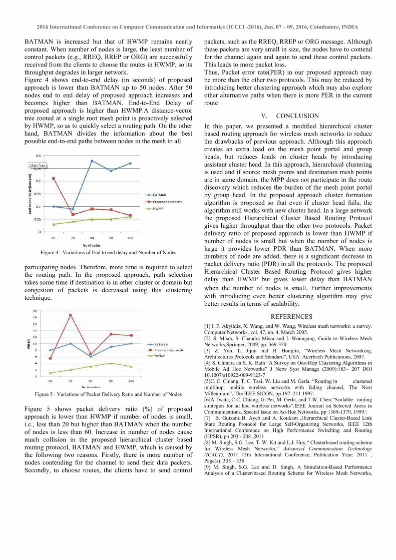
2016 International Conference on Computer Communication and Informatics (ICCCI -2016), Jan. 07 – 09, 2016, Coimbatore, INDIA
BATMAN is increased but that of HWMP remains nearly constant. When number of nodes is large, the least number of control packets (e.g., RREQ, RREP or ORG) are successfully received from the clients to choose the routes in HWMP, so its throughput degrades in larger network. Figure 4 shows end-to-end delay (in seconds) of proposed approach is lower than BATMAN up to 50 nodes. After 50 nodes end to end delay of proposed approach increases and becomes higher than BATMAN. End-to-End Delay of proposed approach is higher than HWMP.A distance-vector tree rooted at a single root mesh point is proactively selected by HWMP, so as to quickly select a routing path. On the other hand, BATMAN divides the information about the best possible end-to-end paths between nodes in the mesh to all
Figure 4 : Variations of End to end delay and Number of Nodes
participating nodes. Therefore, more time is required to select the routing path. In the proposed approach, path selection takes some time if destination is in other cluster or domain but congestion of packets is decreased using this clustering technique.
Figure 5 : Variations of Packet Delivery Ratio and Number of Nodes
Figure 5 shows packet delivery ratio (%) of proposed approach is lower than HWMP if number of nodes is small, i.e., less than 20 but higher than BATMAN when the number of nodes is less than 60. Increase in number of nodes cause much collision in the proposed hierarchical cluster based routing protocol, BATMAN and HWMP, which is caused by the following two reasons. Firstly, there is more number of nodes contending for the channel to send their data packets. Secondly, to choose routes, the clients have to send control
packets, such as the RREQ, RREP or ORG message. Although these packets are very small in size, the nodes have to contend for the channel again and again to send these control packets. This leads to more packet loss. Thus, Packet error rate(PER) in our proposed approach may be more than the other two protocols. This may be reduced by introducing better clustering approach which may also explore other alternative paths when there is more PER in the current route
V. CONCLUSION
In this paper, we presented a modified hierarchical cluster based routing approach for wireless mesh networks to reduce the drawbacks of previous approach. Although this approach creates an extra load on the mesh point portal and group heads, but reduces loads on cluster heads by introducing assistant cluster head. In this approach, hierarchical clustering is used and if source mesh points and destination mesh points are in same domain, the MPP does not participate in the route discovery which reduces the burden of the mesh point portal by group head. In the proposed approach cluster formation algorithm is proposed so that even if cluster head fails, the algorithm still works with new cluster head. In a large network the proposed Hierarchical Cluster Based Routing Protocol gives higher throughput than the other two protocols. Packet delivery ratio of proposed approach is lower than HWMP if number of nodes is small but when the number of nodes is large it provides lower PDR than BATMAN. When more numbers of node are added, there is a significant decrease in packet delivery ratio (PDR) in all the protocols. The proposed Hierarchical Cluster Based Routing Protocol gives higher delay than HWMP but gives lower delay than BATMAN
when the number of nodes is small. Further improvements
with introducing even better clustering algorithm may give better results in terms of scalability.
REFERENCES
[1] I. F. Akyildiz, X. Wang, and W. Wang, Wireless mesh networks: a survey. Computer Networks, vol. 47, no. 4, March 2005. [2] S. Misra, S. Chandra Misra and I. Woungang, Guide to Wireless Mesh Networks,Springer, 2009, pp. 369-370. [3] Z. Yan, L. Jijun and H. Honglin, “Wireless Mesh Networking, Architectures Protocols and Standard”, USA: Auerbach Publications, 2007. [4] S. Chinara an S. K. Rath “A Survey on One-Hop Clustering Algorithms in Mobile Ad Hoc Networks” J Netw Syst Manage (2009):183– 207 DOI 10.1007/s10922-009-9123-7 [5]C. C. Chiang, T. C. Tsai, W. Liu and M. Gerla. “Routing in clustered multihop, mobile wireless networks with fading channel, The Next Millennium”, The IEEE SICON, pp.197–211 1997. [6]A. Iwata, C.C. Chiang, G. Pei, M. Gerla, and T.W. Chen.“Scalable routing strategies for ad hoc wireless networks”.IEEE Journal on Selected Areas in Communications, Special Issue on Ad-Hoc Networks, pp 1369-1379, 1999.\ [7] B. Guizani,.B. Ayeb and A. Koukam ,Hierarchical Cluster-Based Link State Routing Protocol for Large Self-Organizing Networks, IEEE 12th International Conference on High Performance Switching and Routing (HPSR), pp 203 - 208 ,2011 [8] M. Singh, S.G. Lee, T. W. Kit and L.J. Huy,“ Clusterbased routing scheme for Wireless Mesh Networks,” Advanced Communication Technology (ICACT), 2011 13th International Conference, Publication Year: 2011 , Page(s): 335 – 338. [9] M. Singh, S.G. Lee and D. Singh, A Simulation-Based Performance Analysis of a Cluster-based Routing Scheme for Wireless Mesh Networks,

2016 International Conference on Computer Communication and Informatics (ICCCI -2016), Jan. 07 – 09, 2016, Coimbatore, INDIA
International Journal of Multimedia and Ubiquitous Engineering, Vol.8, No.5 ,2013, pp.283-296. [10] D. Kaushal, G. Niteshkumar, B. Prasann K. and V. Agarwal. Hierarchical cluster based routing for wireless mesh networks using group head, International Conference on Computing Sciences (ICCS), Phagwara, pp. 163-167, 2012. [11]Neumann, C. Aichele, M. Lindner, and S. Wunderlich, Better Approach To Mobile Ad-hoc Networking (B.A.T.M.A.N.), Internet-Draft, pages 1-24, 2008. Network Working Group [12] S. M. S. Bari, F. Anwar, M. H. Masud, Performance Study of Hybrid Wireless Mesh Protocol (HWMP) for IEEE 802.11s WLAN Mesh Networks, International Conference on Computer and Communication Engineering ,July 2012, pp. 712-716. [13] A H Mozumder, T Acharjee, S Roy, Scalability performance analysis of batman and HWMP protocols in wireless mesh networks using ns-3, International Conference On Green Computing Communication and Electrical Engineering (ICGCCEE), 2014 , pp. 1–5. [14] NS-3, The ns3 network simulator, *Online+. Available: http://www.nsnam.org/, 2014.

An Ontology Based Context Aware
Protocol in Healthcare Services
Anirban Chakrabarty and Sudipta Roy
Abstract Interpretation of medical document requires descriptors to define
semantically meaningful relations but due to the ever changing demands in
healthcare environment such information sources can be highly dynamic. In these
situations the most challenging problem is frequent ontology search keeping with
user’s interest. To manage this problem efficiently the paper suggests an ontology
model using context aware properties of the system to facilitate the search process
and allow dynamic ontology modification. The proposed method has been evalu-
ated on Cancer datasets collected from publicly accessible sites and the results
confirm its superiority over well known semantic similarity measures.
Keywords Ontology mapping ⋅ Context awareness ⋅ Search personalization ⋅Healthcare
1 Introduction
Most Healthcare systems contain a large collection of related documents which
necessitates a semantic search system to swiftly and accurately identify documents
which satisfy user’s needs. It has been found that keyword based search engines
most often fail to give the expected results relevant to the query context. One of the
key factors for personalized information access is the user context [1]. Context can
be defined as the user’s objective for seeking information [2]. In this paper, context
is defined through the notion of ontological profiles which are updated over time to
reflect changes in user interests. Ontology consists of a formal conceptualization in
a particular field of interest that can be easily visualized or can be considered as a
Anirban Chakrabarty (✉) ⋅ Sudipta Roy
Assam Central University, Silchar, India
e-mail: [email protected]
Sudipta Roy
e-mail: [email protected]
© Springer Science+Business Media Singapore 2017
J.K. Mandal et al. (eds.), Proceedings of the First International Conference
on Intelligent Computing and Communication, Advances in Intelligent Systems
and Computing 458, DOI 10.1007/978-981-10-2035-3_15
137

description of the elements it contains and when aligned with other ontologies it can
help in forming a community of such elements or concepts [3, 4].
The major contributions suggested in this paper is mentioned as follows: (1) It
provides an ontology for cancer patients containing both medical and socio eco-
nomic conditions (2) to search for an optimal treatment plan suited to the patient
(3) The ontology can be extended by healthcare experts based on changing treat-
ment options, different disease symptoms and missing information with minimum
involvement from external sources. (4) An ontology mapping strategy has been
suggested that exploits contextual information of source ontology and supplements
it in linguistic and structural similarity to enhance the strength of match with the
target ontology.
2 Related Work
Most retrieval systems suffer from keyword barrier phenomenon which refers to the
inability of information retrieval systems to convey semantic context of documents
[5]. Related work developed a framework for Formal Concept Analysis which
extended the Tf-Idf weighting model by introducing ontology dependent concepts
[6]. Most search engines do not include user preferences and search context but
provide users with a generalized search facility [7]. A related study shows that little
work has been done on contextual retrieval to combine search technologies and
ontology alignment using context in a single framework to provide the most
accurate response for a user’s information requirement [8].
A popular method to facilitate information access is through the use of ontology.
Researchers have attempted to utilize ontology for improving navigation effec-
tiveness as well as personalized Web search and browsing for generating user
profiles [9]. An innovative approach for Ontology based on Concept merging was
suggested were first the horizontal technique checks all relationships between
concepts at the same level of two ontologies and merges them as defined by
WordNet, then the vertical approach completes the merging of concepts at different
levels but placed on same branch of the tree [10].
The notion of concept similarity calculation using ontology is that two concepts
have a semantic correlation, and there exists a path in class hierarchy diagram. In a
pioneering work, Resnik measures the semantic similarity of two words according
to the maximum amount of information of their common ancestor node [11].
Leacock and Chodorow proposed a semantic similarity model based on distance
which is an easy and natural approach but is heavily dependent on the ontology
hierarchy already established [12]. Study of related work shows the use of RIMOM:
a dynamic multi strategy ontology alignment framework which uses both linguistic
and structural similarity to map source and target ontologies but it is suitable for
only for 1:1 mapping [13]. The ontologies can be expressed in various ways. The
most common language used to model ontologies is the Web Ontology Language
(OWL), which is a form of RDF and is written using a subset of XML [14].
138 Anirban Chakrabarty and Sudipta Roy

Unfortunately, most of these systems can provide little support in support for
knowledge sharing and context reasoning because of their lack of ontology. Recent
study focus on the use ontology based personalization system for assisting
healthcare industry in patient diagnosis and intervention plans [15].
3 Methodology
In this work ontology has been developed to organize the terms of cancer disease,
its symptoms, diagnosis, treatment options, intervention plans, patient condition
and other social issues related to disease. On top of this a search algorithm based on
context information stored in Ontology has been suggested which extracts all
correlated words of the search string and can map from one ontology to another
(Figs. 1 and 2).
Fig. 1 Flowchart of context matching using an ontology framework
An Ontology Based Context Aware Protocol in Healthcare Services 139

4 Ontology Used
There are many existing ontology, but since critically ill patients need accurate and
urgent medical intervention we have developed Cancer related Ontology containing
medical and social concepts to assist in searching information and decision making.
5 Explanation of Proposed Algorithms
5.1 Context Search Technique
Step 1 Perform linguistic match between search string and the one present in
target ontology based on Word Net. If direct match is found then display
output and exit.
If no direct match found then based on the similarity results the pairs are
sorted into three buckets: (a) above the upper threshold—provisionally
similar (b) between the upper and lower threshold—uncertain bucket and
(c) below the lower threshold—no match. Add all composite matches to
the “uncertain bucket” along with the concepts between the upper and
lower threshold (selected based on experimentation).
Step 2 Structural matching: For concepts whose similarity values are in uncertain
bucket, perform the following:
Fig. 2 Ontology hierarchy for cancer patients
140 Anirban Chakrabarty and Sudipta Roy

(a) for each pair of concept, compare their parent nodes (when matching is
between two ontology) to determine the total parental similarity for
updating the original pairs similarity value. If match is found incre-
ment the score by 0.1.
(b) for each pair of concepts, compare their grandparent nodes to deter-
mine the total similarity for updating the original pairs similarity value.
If match is found increment the score by 0.05.
Step 3 Use Word Sense disambiguation on the set of terms in ‘Uncertain’ and
‘Provisionally similar’ buckets to select the words actually representing the
given context. The WSD method used here takes average of similarity
values for each concept searched to show its relatedness to the ontology.
5.2 Ontology Modification
This procedure is called when the context is not found in the ontology tree but the
searched context has a comparable relation then the context is dynamically added as
a node in the ontology tree in appropriate location. Each ontology node is asso-
ciated with an Id for comparison.
Pseudo code:
Modify (Root,Id,mi,N,M,Left,Right,Par)
Set Ptr = Root, Id= TRUE.
Apply Algorithm-2 to find the similarity or relevance of searched area.
[If Node found] Set Ptr=Node.
Else if [node was not found but has to be added based on relevance threshold of the
domain set then check immediate ancestor. ]
{ Id[NodeO1]->Par=Id [NodeO2]->Par
Add new node.
If{ Id [NodeO1]<Id [NodeO1]->Par
Set Left[Par]=New
Else Set Right[Par]=New.
Set Id of new node.}
Print Updation Successful.
}}
[Else Updation Not Possible. ]
}
An Ontology Based Context Aware Protocol in Healthcare Services 141

6 Experiment
6.1 Data Set
The experimental data used in this work has been collected from different cancer
related websites which allows open access and made publicly available for research
and study purposes [16–21]. The training data set comprising of 2721 documents
was used for the representation of the cancer ontology indexing 204 concepts in the
hierarchy.
6.2 Experimental Metrics
To perform a comparison of the improvement of proposed method with other
established semantic search algorithms used in contemporary literature like k-NN,
Resnik similarity, Rocchio based methods [22, 23].
The similarity measure suggested by Resnik, gives the information content
(IC) of the Least Common Subsequence (LCS) for two concepts:
SimRes = IC(LCS) ð6Þ
where IC is defined as:
IC(c) = − log p(c) ð7Þ
here p(c) is the probability of encountering a context c in a corpus.
F-M
easu
re
Fig. 3 Comparison of F-measure with other similarity measures for five users
142 Anirban Chakrabarty and Sudipta Roy

The effectiveness of search was measured in terms of Top-n Recall and Top-n
Precision [24]. The F-measure defined as F = 2 * P * R/(P + R) is a balanced
mean between precision and recall metrics and was used for comparing searches
made by five different users.
6.3 Results
See Figs. 3, 4, 5 and 6.
F-M
easu
re
Threshold
Fig. 4 Comparison of F-measure with varying threshold
Documents
Top-n
Recall
Fig. 5 Variation of average top-n recall in top-n documents using overlap queries
An Ontology Based Context Aware Protocol in Healthcare Services 143
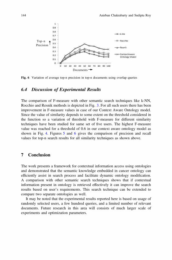
6.4 Discussion of Experimental Results
The comparison of F-measure with other semantic search techniques like k-NN,
Rocchio and Resnik methods is depicted in Fig. 3. For all such users there has been
improvement in F-measure values in case of our Context Aware Ontology model.
Since the value of similarity depends to some extent on the threshold considered in
the function so a variation of threshold with F-measure for different similarity
techniques have been studied for same set of five users. The highest F-measure
value was reached for a threshold of 0.6 in our context aware ontology model as
shown in Fig. 4. Figures 5 and 6 gives the comparison of precision and recall
values for top-n search results for all similarity techniques as shown above.
7 Conclusion
The work presents a framework for contextual information access using ontologies
and demonstrated that the semantic knowledge embedded in cancer ontology can
efficiently assist in search process and facilitate dynamic ontology modification.
A comparison with other semantic search techniques shows that if contextual
information present in ontology is retrieved effectively it can improve the search
results based on user’s requirements. This search technique can be extended to
compare two separate ontologies as well.
It may be noted that the experimental results reported here is based on usage of
randomly selected users, a few hundred queries, and a limited number of relevant
documents. Future research in this area will consists of much larger scale of
experiments and optimization parameters.
Documents
Top-n
Precision
Fig. 6 Variation of average top-n precision in top-n documents using overlap queries
144 Anirban Chakrabarty and Sudipta Roy

References
1. Pei-Min Chen, Fong-Chou Kuo , An information retrieval system based on a user profile, The
Journal of Systems and Software, vol. 54, pp. 3–8, 2000.
2. Dey, A.K., Salber, D. Abowd, G.D., “A Conceptual Framework and a Toolkit for Supporting
the Rapid Prototyping of Context-Aware Applications”, Human-Computer Interaction
Journal, Vol. 16(2–4), pp. 97–166, 2001.
3. Cimiano, P., Ontology Learning and Population from Text: Algorithms, Evaluation and
Applications. Springer-Verlag New York, Inc., Secaucus, NJ, USA, 2006.
4. Gargouri, Y., Lefebvre, B., Meunier, J. Ontology Maintenance using Textual Analysis.
Proceedings of the Seventh World Multi-Conference on Systemics, Cybernetics and
Informatics (SCI). Orlando, USA (2003).
5. M-Y. Chen, H-C. Chu, Y-M. Chen, Developing a semantic enable information retrieval
mechanism. Expert Systems with Applications, 37:322–340, 2010.
6. Rohana K. Rajapakse, Michael. Denham, Text retrieval with more realistic concept matching
and reinforcement learning. Information Processing and Management. 42(5), 1260–127,
September 2006.
7. Ashraf, J., Khadeer Hussain, O., Khadeer Hussain, F.: A Framework for Measuring Ontology
Usage on the Web. In: The Computer Journal. Oxford University Press, 2012.
8. J. Allan, et al. Challenges in information retrieval and language modeling. ACM SIGIR
Forum, 37(1):31–47, 2003.
9. Fang Liu, Clement Yu, Personalized Web Search for Improving Retrieval Effectiveness, IEEE
Transactions on Knowledge and Data Engineering, Vol. 16, No. 1, January 2004.
10. Miyoung Cho, Hanil Kim, and Pankoo Kim. A new method for ontology merging based on
concept using wordnet. In Advanced Communication Technology, 2006. ICACT 2006. The
8th International Conference, volume 3, pages 1573/1576, February 2006.
11. Philip Resnik, “Using Information Content to Evaluate Semantic Similarity in a taxonomy”, In
Proceedings of the 14th International Joint Conference on Artificial Intelligence. Monte real,
Canada, pp. 448–453, 1995.
12. C. Leacock, M. Chodorow. “Combining Local Context and WordNet Similarity for Word
Sense Identification”, Computational Linguistics, vol. 24, no. 1, pp. 147–165, 1998.
13. Juanzi Li, Jie Tang, Yi Li, and Qiong LuoRiMOM: A Dynamic Multistrategy Ontology
Alignment Framework, IEEE Transactions on Knowledge and Data Engineering, Vol. 21,
No. 8, August 2009.
14. Ashraf, J., Khadeer Hussain, O., Khadeer Hussain, F.: A Framework for Measuring Ontology
Usage on the Web. In: The Computer Journal. Oxford University Press, 2012.
15. David Riano; Francis Real; Joan Albert Lopez; Fabio Campana; Sara Ercolani; Patrizia
Mecocci; Roberta Annicchiarico & Carlo Caltagirone. An Ontology based personalization of
Healthcare knowledge to support clinical decisions for chronically ill patients, Journal of
Biomedical Informatics, Elsevier, 429–446, 45 (2012).
16. http://www.cancer.org/research/index [Last accessed on 12th October, 2015].
17. http://www.cancercare.org/accessengagementreport [Last accessed on 12th October 2015].
18. http://www.oncolink.org/resources [Last accessed on 7th October, 2015].
19. http://med.stanford.edu/cancer.html [Last accessed on 25th September, 2015].
20. http://www.ncbi.nlm.nih.gov/pubmed [Last accessed on 21st September, 2015].
21. http://www.cdc.gov/cancer/ [Last accessed on 16th September, 2015].
22. Oh-Woog Kwon, Jong Hyeok Lee. Text categorization based on k-nearest neighbor approach
for Web site classification, Information Processing and Management Volume 39, Issue 1,
Pages 25–44, January 2003.
An Ontology Based Context Aware Protocol in Healthcare Services 145

23. Guanyu Gao, Shengxiao Guan. Text categorization based on improved Rocchio algorithm. In
Proc. of Systems and Informatics (ICSAI) IEEE International Conference, pp. 2247–2250,
2012.
24. Paulo Cremonesi, Yehuda Koren, Roberto Turrin. Performance of recommender algorithms on
top-n recommendation tasks. In Proc. of the fourth ACM conference on Recommender
Systems, pp. 39–46, ACM New York, USA, 2010.
146 Anirban Chakrabarty and Sudipta Roy

Classification and Performance Analysis of Intra-domainMobility Management Schemes for Wireless Mesh Network
Abhishek MajumderTripura University
Suryamaninagar, Agartala
Subhrajyoti DebTripura University
Suryamaninagar, Agartala
Sudipta RoyAssam UniversitySilchar, Assam
ABSTRACT
Nowadays Wireless Mesh Networks (WMNs) has come upwith a promising solution for modern wireless communica-tions. But, one of the major problems with WMN is the mo-bility of the Mesh Clients (MCs). To offer seamless connec-tivity to the MCs, their mobility management is necessary.During mobility management one of the major concerns isthe communication overhead incurred during handoff of theMCs. For addressing this concern, many schemes have beenproposed by the researchers. In this paper, a classificationof the existing intra domain mobility management schemeshas been presented. The schemes have been numerically an-alyzed. Finally, their performance has been analyzed andcompared with respect to handoff cost considering differentmobility rates of the MCs.
Categories and Subject Descriptors
C.2.1 [Network Architecture and Design]: Wireless com-munication
General Terms
Numerical Analysis
Keywords
Wireless Mesh Networks, Mobility Management, Intra-domain,Mesh Client, Handoff, Classification
1. INTRODUCTIONRecently Wireless Mesh Networks (WMNs) has become
a prominent solution for modern wireless communications.In WMN nodes can be classified as mesh client (MC), meshrouter (MR) and gateway (GW). The mobile users are MCs.MRs are the wireless routers to route the Internet as wellas intranet packets. An MR having a wired interface tothe Internet is called GW. Because of the random mobilitybehavior of the MC maintenance of seamless network con-nectivity becomes a challenging issue. In last few years some
Permission to make digital or hard copies of all or part of this work forpersonal or classroom use is granted without fee provided that copies arenot made or distributed for profit or commercial advantage and that copiesbear this notice and the full citation on the first page. To copy otherwise, torepublish, to post on servers or to redistribute to lists, requires prior specificpermission and/or a fee. Request permissions from [email protected]’16 March 4-5, 2016, Udaipur, Rajasthan, India.c© 2016 ACM. ISBN 978-1-4503-3962-9/16/03 ...$15
http://dx.doi.org/10.1145/2905055.2905173.
broad surveys on mobility management in cellular networkshave been carried out and various models have already beenestablished for analysis of performance. But due to architec-tural difference the proposed schemes are generally not rele-vant for WMNs [1]. In [1] I.F. Akyildiz et al explained thatbecause of distributed nature of the WMN the mobility man-agement designed for centralized cellular network cannot beused in WMN. The mobility management schemes designedfor ad-hoc network does not work well in WMN because inWMN the MRs are generally static and the MCs are mobile.In case of ad-hoc network all the nodes are mobile. This gapcreates the opportunity of development of mobility manage-ment schemes for WMN considering its unique feature ofalmost static MRs. For providing seamless connectivity tothe MCs in WMN many mobility management schemes havebeen developed. Some of the intra-domain mobility manage-ment schemes discussed in this paper are: MEsh networkswith MObility management (MEMO) [2], Mesh MobilityManagement (M3) [3], and Wireless mesh Mobility Man-agement (WMM) [4], ANT [5], Infrastructure Mesh (iMesh)[4], SMesh[7], Static Anchor Scheme [8] and Dynamic An-chor Scheme [8] have been discussed. The schemes havebeen classified considering the approach they use to routethe packets. Finally, the schemes are numerically analyzedto observe the effect of mobility rate of MCs on handoff cost.
Organization of the paper is as follows. Section 2 dis-cusses the classification of intra-domain mobility manage-ment. In section 3 System model and assumptions havebeen discussed. The mobility management schemes havebeen numerically analyzed in section 4. Section 5 comparesthe performance of the schemes. Finally, conclusion has beenpresented in section 6.
2. INTRA-DOMAIN MOBILITY MANAGE-
MENTIn mobility management there are two parts: location
management and handoff management [1]. Location man-agement manages the location registration and this issue hasbeen comprehensively researched for cellular networks. Mo-bile terminals periodically send the information to the sys-tem that update new location details in location database[9]. On the other hand, handoff management is a mech-anism where terminals carry all its connections active oralive while shifting to another access pint (AP) from its cur-rent AP. A comprehensive literature study of mobility man-agement in wireless mesh networks has discussed in [1, 10,11]. There are two types of mobility management schemesin WMN: intra-domain mobility management scheme and
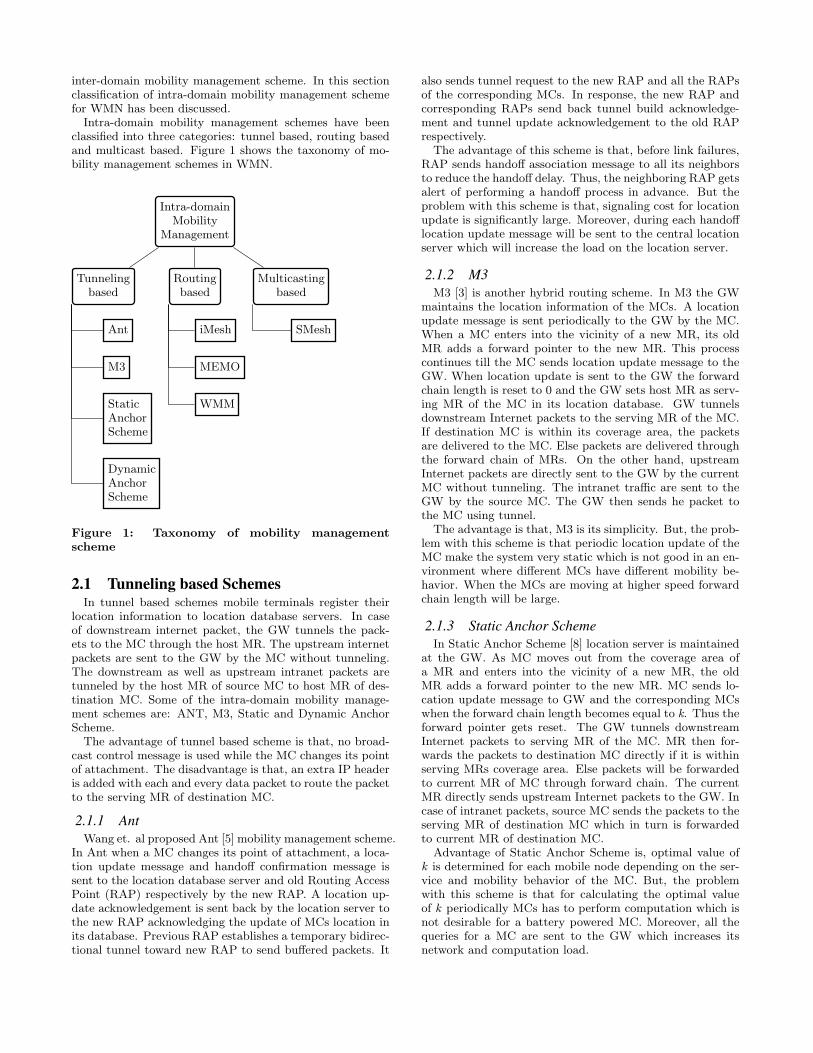
inter-domain mobility management scheme. In this sectionclassification of intra-domain mobility management schemefor WMN has been discussed.
Intra-domain mobility management schemes have beenclassified into three categories: tunnel based, routing basedand multicast based. Figure 1 shows the taxonomy of mo-bility management schemes in WMN.
Intra-domainMobility
Management
Tunnelingbased
Ant
M3
StaticAnchorScheme
DynamicAnchorScheme
Routingbased
iMesh
MEMO
WMM
Multicastingbased
SMesh
Figure 1: Taxonomy of mobility managementscheme
2.1 Tunneling based SchemesIn tunnel based schemes mobile terminals register their
location information to location database servers. In caseof downstream internet packet, the GW tunnels the pack-ets to the MC through the host MR. The upstream internetpackets are sent to the GW by the MC without tunneling.The downstream as well as upstream intranet packets aretunneled by the host MR of source MC to host MR of des-tination MC. Some of the intra-domain mobility manage-ment schemes are: ANT, M3, Static and Dynamic AnchorScheme.
The advantage of tunnel based scheme is that, no broad-cast control message is used while the MC changes its pointof attachment. The disadvantage is that, an extra IP headeris added with each and every data packet to route the packetto the serving MR of destination MC.
2.1.1 Ant
Wang et. al proposed Ant [5] mobility management scheme.In Ant when a MC changes its point of attachment, a loca-tion update message and handoff confirmation message issent to the location database server and old Routing AccessPoint (RAP) respectively by the new RAP. A location up-date acknowledgement is sent back by the location server tothe new RAP acknowledging the update of MCs location inits database. Previous RAP establishes a temporary bidirec-tional tunnel toward new RAP to send buffered packets. It
also sends tunnel request to the new RAP and all the RAPsof the corresponding MCs. In response, the new RAP andcorresponding RAPs send back tunnel build acknowledge-ment and tunnel update acknowledgement to the old RAPrespectively.
The advantage of this scheme is that, before link failures,RAP sends handoff association message to all its neighborsto reduce the handoff delay. Thus, the neighboring RAP getsalert of performing a handoff process in advance. But theproblem with this scheme is that, signaling cost for locationupdate is significantly large. Moreover, during each handofflocation update message will be sent to the central locationserver which will increase the load on the location server.
2.1.2 M3
M3 [3] is another hybrid routing scheme. In M3 the GWmaintains the location information of the MCs. A locationupdate message is sent periodically to the GW by the MC.When a MC enters into the vicinity of a new MR, its oldMR adds a forward pointer to the new MR. This processcontinues till the MC sends location update message to theGW. When location update is sent to the GW the forwardchain length is reset to 0 and the GW sets host MR as serv-ing MR of the MC in its location database. GW tunnelsdownstream Internet packets to the serving MR of the MC.If destination MC is within its coverage area, the packetsare delivered to the MC. Else packets are delivered throughthe forward chain of MRs. On the other hand, upstreamInternet packets are directly sent to the GW by the currentMC without tunneling. The intranet traffic are sent to theGW by the source MC. The GW then sends he packet tothe MC using tunnel.
The advantage is that, M3 is its simplicity. But, the prob-lem with this scheme is that periodic location update of theMC make the system very static which is not good in an en-vironment where different MCs have different mobility be-havior. When the MCs are moving at higher speed forwardchain length will be large.
2.1.3 Static Anchor Scheme
In Static Anchor Scheme [8] location server is maintainedat the GW. As MC moves out from the coverage area ofa MR and enters into the vicinity of a new MR, the oldMR adds a forward pointer to the new MR. MC sends lo-cation update message to GW and the corresponding MCswhen the forward chain length becomes equal to k. Thus theforward pointer gets reset. The GW tunnels downstreamInternet packets to serving MR of the MC. MR then for-wards the packets to destination MC directly if it is withinserving MRs coverage area. Else packets will be forwardedto current MR of MC through forward chain. The currentMR directly sends upstream Internet packets to the GW. Incase of intranet packets, source MC sends the packets to theserving MR of destination MC which in turn is forwardedto current MR of destination MC.
Advantage of Static Anchor Scheme is, optimal value ofk is determined for each mobile node depending on the ser-vice and mobility behavior of the MC. But, the problemwith this scheme is that for calculating the optimal valueof k periodically MCs has to perform computation which isnot desirable for a battery powered MC. Moreover, all thequeries for a MC are sent to the GW which increases itsnetwork and computation load.

2.1.4 Dynamic Anchor Scheme
This scheme is similar to the Static Anchor Scheme buthere only difference is that in addition to the previous con-dition the forward pointer will be reset due to arrival of newintranet or Internet session. When the new Internet sessionarrives, the GW sends location query message to the MCthrough the serving MR of the MC. The current MR of theMC sends back response to the GW and the forward chaingets reset. In case of arriving intranet session, the sourceMC ends location query message for the destination MC tothe GW. The GW performs the same location query processas it has done in case of Internet session arrival. After the lo-cation of the MC is updated in the GW, the GW sends backthe response to the source MC. The source MC the thensend packet directly to the serving MR of the destinationMC.
The advantage of this scheme is that, the schemes is be-haves more dynamically in different network conditions. Theproblem with this scheme is that the load on the GW in-creases heavily.
2.2 Routing based SchemeRouting based schemes combine routing protocol with mo-
bility management. MCs location information is propagatedall through the WMN using routing scheme. Some of therouting based intra-domain mobility management schemesare: iMesh, MEMO and WMM.
In general the advantage routing based scheme is that noextra IP header is necessary for routing of data packets todestination MCs. Problem with this type of scheme is routeupdate message is broadcasted in entire WMN.
2.2.1 iMesh
In iMesh [6] when MC enters into the vicinity of new MR,its route information is broadcasted in entire WMN throughHost and Network Association (HNA) message. OLSR rout-ing protocol is used for this broadcast. On receiving HNAall the MRs update MCs routing information.
Advantage of this scheme is that use of OLSR for broad-casting HNA message reduces the propagation of controlmessages. The problem with this scheme is that, HNA mes-sage is broadcasted after every handoff.
2.2.2 MEMO
In MEMO [2] scheme, as MC changes its point of attach-ment route error message is broadcasted in entire WMN byold MR. New MR proactively sends route reply message toGW for Internet communication. To maintain ongoing in-tranet connectivity the new MR broadcasts route requestmessage to find a path to the corresponding MCs. In re-sponse, MRs of corresponding MCs send back route reply.This scheme uses routing table entries for routing of Internetand intranet packets.
The advantage of this scheme is that for maintaining con-tinuous Internet connectivity a route reply message is proac-tively sent to the GW by the MC. Moreover, routing processis straight forward in this scheme. But the problem with thisscheme is that excessive propagation of control message forremoval of old route and setting up of new route.
2.2.3 WMM
Huang et al. introduced WMM scheme [4]. In WMM,MR maintains two types of table: routing table and proxy
table. In this scheme no location update message is used.The options field of IP header of the data packet is dividedinto four parts: IRS (IP address of receivers host MR), RST(timestamp of senders host MR), ISS (IP address of sendershost MR) and SST (timestamp of senders host MR). The ISSstores the IP address of MCs current MR. While forward-ing data packets the intermediate MRs store the address ofsource MCs current MR in its proxy table. When a MCenters into the vicinity of a new MR, the old MR adds aforward pointer towards new MR.
The advantage of this scheme is that unlike other routingbased scheme it does not suffer from excessive propagationof control message for route management. The problem ofthis scheme is that, each data packet has to carry extra bytesfor storing IRS, RST, ISS and SST in its IP header.
2.3 Multicasting based SchemesIn Multicast based scheme a MC may be associated with
a multiple MRs at a time. Data packets destined to MCs arecopied and multi-casted to all the MRs in MCs data group.
The advantage of this type of scheme is that, this schemereduces the handoff latency by associating MC with multipleMRs. On the other hand it suffers from routing overheadbecause of multicasting of the packets.
2.3.1 SMesh
In SMesh [10] there are two groups of MRs associated witha MC: data group and control group. A MR which believesthat it can serve a MC the best, it joins the data group ofthat MC. The MRs of the control group will keep track ofthe MCs current location. When there is some packet to bedelivered to the MC, it is multicasted to all the MRs whichare in the data group of the MC. On receiving those packets,the MRs forward the packets to the MC.
The advantage of this scheme is that, because of multicas-ting possibility of packet is low. But, before the MC movesto the neighboring MR, the current MR establishes tunnelto all the neighboring MRs. This requires significant num-ber of control packet transfer. Moreover, for maintenance ofmulticast group huge routing overhead is involved.
3. SYSTEM MODELThis section presents system model and assumptions for
carrying out the numerical analysis. Let, residence time ofthe MC in a MRs coverage area follows exponential distri-bution with rate (ts) [12]. Therefore, the number of asso-ciations of an MC with MRs in a time unit follows Pois-son distribution with rate λs [12]. In addition to the abovementioned assumptions some more parameters are used fornumerical analysis of the schemes. Table 1 shows the pa-rameters used for mathematical modeling and their inter-pretations.
4. NUMERICAL ANALYSISIn this section handoff cost of intra-domain mobility man-
agement schemes discussed in section 2 will be discussed. InAnt scheme, when the MC moves from one RAP (Rout-ing Access Point) to another, new RAP sends location up-date message towards location server. When location serverreceives location update message, it updates its locationdatabase and sends back location update acknowledgement.Old RAP sends tunnel setup request to the new RAP and

Symbol Interpretation
M Total number of MRs in the WMN.
αAverage distance between an arbitraryMR and the GW.
βAverage distance from an arbitrary MR toanother arbitrary MR in WMN.
γ Communication latency per hop.
tM3
Time interval between two consecutivelocation updates in M3.
NactiveAverage number of corresponding MCs ofany arbitrary MC.
kThreshold forward chain length for reset of forwardchain in Static and Dynamic Anchor Scheme.
cmove Average displacement of MC per MR association.
PrProbability that the MR broadcasts networkcontrol message to its neighborhood.
Table 1: Parameters and their interpretations.
the RAPs of corresponding nodes. The new RAP and corre-sponding RAPs sends tunnel build ACK and tunnel updateACK to the old RAP. So handoff cost per time unit of thescheme is,
ChANT = {(2× α+ 2× β ×Nactive + 2)× γ}×λs (1)
In SMesh as client moves from old mesh node to a newmesh node, it joins the data group of the client and thelocal spines deamon informs all the other nodes of the meshnetwork through flooding. The old mesh node sends leaverequest to the control group of the client. The mesh nodebelieving that it has the best connection with client sendsback an acknowledgement. The local spines deamon informsother mesh node about its leave information from the datagroup of client. Therefore, the handoff cost per time unit is,
ChsMesh = (2×M × Pr + 2× γ)×λs (2)
In case of static anchor scheme [8] and dynamic anchorpoint scheme [8] location update message of the mesh clientis sent to the Location server when the forward chain lengthis k. The cost of the procedure is (α+Nactive × β)× γ.Else,old Anchor Mesh Router adds a forward pointer to new An-chor Mesh Router costing 2× γ. Therefore, handoff cost pertime unit is,
Chstatic = Chdynamic = {2 × γ ×
(
λs −λs×Cmove
k
)
+ (α +
Nactive × β)× λs×Cmove
k× γ} (3)
In iMesh as MC moves from one MR to another, HNAmessage is broadcasted using OLSR. So, handoff cost pertime unit is,
ChiMesh = {Pr +M}×λs(4)
In MEMO scheme when MC changes its point of attach-ment from one MR to different MR, route error message isbroadcasted in entire network by the old MR. A proactiveroute reply is sent towards GW by the MC. If MC wishes toextend the communication with corresponding MC, the newMR broadcasts route requests in WMN for finding corre-sponding MC. The host MR of corresponding MC respondsby sending back route reply. Therefore, the schemes handoffcost per time unit is [12],
ChMEMO = {M + α× γ +Nactive × (M + β × γ)}×λs (5)
In M3 scheme location update message is sent by the MCto GW every tM3 time unit. Else, old MR adds a forwardpointer to new MR. So the per time unit handoff cost is [12],
ChM3 = {2× γ × tM3−1
tM3
+ α× γ × 1
tM3
}×λs(6)
In WMM scheme there is no separate location update mes-sage. As MC changes its point of attachment, old MR addsa forward pointer to new MR. So, per time unit handoff costis computed as [12],
ChWMM = {2× γ}×λs(7)
5. PERFORMANCE COMPARISONIn this section, the handoff cost of all the schemes which
are numerically analyzed in section 4 has been compared.Table 2 shows the typical values of parameters used for com-parison.
Parameter ValueM 1000α 50β 30γ 0.1k 10tm3 1200cmove[12] 0.4Pr 0.4
Table 2: Value assign for handoff cost calculation
Figure 2 shows the effect of increase in mobility rate onhandoff cost. Here, the value of Nactive is considered as 30and the value of λs is varied between 0.05 and 0.5. Fromfigure 2 it can be observed that handoff cost per time unit

Figure 2: Impact of mobility rate on handoff costper time unit
of MEMO is the highest among all the schemes. This is be-cause in MEMO during every handoff route error and routerequest messages are broadcasted. Figure 3 shows a sub-graph of figure 2 to highlight the effect of mobility rate onhandoff cost per time unit of Ant, Static Anchor Scheme,iMesh, M3 and WMM. SMesh has significantly high handoffcost. The reason behind this is, broadcast of join and leaveinformation in the entire network by the new and old MRrespectively. In iMesh since message is broadcasted in theentire network only by the newMR during every handoff, thehandoff cost is less than SMesh. In case of ANT, only unicastmessage are sent by the old and new MR to the GW and cor-responding MR during every handoff. Therefore, its handoffcost per time unit is less than that of iMesh. In Static andDynamic Anchor Scheme, when the forward chain lengthbecomes equal to k location update message is sent to theGW as well as corresponding MRs. Since here k = 10 thefrequency of sending the location update message is very lesswhich results in a handoff cost very less than that of ANT.In M3 location update message is sent every tM3 time unit.Since, tM3 is set to 1200, MC sends route update messagetowards GW less frequently. Therefore, location update costis less than that of M3. In WMM there is no location updatemessage. Only old MR adds a forward pointer to new MR.Therefore, handoff cost per time unit of WMM is the lowest.With the increases in mobility rate, handoff cost per timeunit of all schemes increases because frequency of sendinglocation update message increases. Increase rate of MEMOis very high because, the scheme uses AODV for flooding ofroute request and the number of route request and route er-ror broadcasts increases with increase in node mobility rate.SMesh increases at lower rate than MEMO, because herelink state routing protocol is used for broadcasting leave andjoin information of MRs in the entire WMN. Rate of increasein handoff cost of iMesh is less than SMesh because here onlyHNA message is broadcasted in WMN using OLSR. Hand-off cost per time unit of Ant increases at lower rate thaniMesh because it uses unicasting of location update messageinstead of broadcasting. The increase rate of Static AnchorScheme, Dynamic Anchor Scheme, M3 and WMM is verylow because the frequency of sending unicast location up-date message is very less.
Figure 3: Impact of mobility rate on handoff costper time unit (Subplot of figure 2)
Figure 4: Impact of number of corresponding nodeson handoff cost per time unit
Figure 5: Impact of number of corresponding nodeson handoff cost per time unit (Subplot of figure 3)
Figure 4 shows the impact of increase in number of corre-sponding nodes (Nactive) on handoff cost per time unit. Fig-ure 5 shows the subplot of figure 4 highlighting the handoffcost for Ant, SMesh, Static Anchor Scheme, Dynamic An-chor Scheme, iMesh, M3 and WMM. Here, the value of λs
is set to 0.25 and the number of corresponding MCs are var-ied between 10 to 100. With the increase in Nactive handoffcost per time unit increases because route request message isbroadcasted in the entire network for more number of cor-responding MCs. The handoff cost of Ant increases withthe increase in Nactive because tunneling request is sent tomore number of MRs. In case of Static and Dynamic An-chor Scheme since location update message sent to the cor-responding MRs is infrequent, handoff cost per time unitincreases at very low rate. Handoff cost of iMesh, M3 andWMM is independent of increase in Nactive because locationupdate message is not sent individually to correspondingMCs.
6. CONCLUSION AND FUTURE WORKThis paper presents classification of mobility management
schemes. Different mobility management schemes have beendiscussed in brief. Handoff cost per time unit of the mobilitymanagement schemes have been calculated. A comparativestudy of the mobility management schemes with respect tohandoff cost has been performed. From the comparison itwas found that MEMO and WMM has the highest and low-est handoff cost per time unit respectively. Study of querycost and packet delivery cost of these schemes remains asfuture work. Moreover, simulation of the mobility manage-ment schemes for comparison will also be done in future.
7. ACKNOWLEDGEMENTThe work is funded by Department of Electronics and In-
formation Technology (DeitY), Ministry of Communicationsand Information Technology, Electronics niketan, 6 CGOComplex, Lodhi Road, New Delhi-110003, Government ofIndia, Vide no. 14(8)/2014-CC&BT, Dated: 03.09.2015.
8. REFERENCES
[1] I. F. Akyildiz, X. Wang, and W. Wang, “Wirelessmesh networks: A survey,” Computer Networks, vol.47, no. 4, pp. 445-487, Mar. 2005.
[2] M. Ren, C. Liu, H. Zhao, T. Zhao, and W. Yan,“MEMO: An applied wireless mesh network withclient support and mobility management,” IEEEGLOBECOM 2007-2007 IEEE GlobalTelecommunications Conference, Nov. 2007.
[3] R. Huang, C. Zhang, and Y. Fang, “A mobilitymanagement scheme for wireless mesh networks,”IEEE GLOBECOM 2007-2007 IEEE GlobalTelecommunications Conference, Nov. 2007.
[4] D.-W. Huang, P. Lin, and C.-H. Gan, “Design andperformance study for a mobility managementmechanism (WMM) using location cache for wirelessmesh networks,” IEEE Transactions on MobileComputing, vol. 7, no. 5, pp. 546-556, May 2008.
[5] H. Wang, Q. Huang, Y. Xia, Y. Wu, and Y. Yuan, “Anetwork-based local mobility management scheme forwireless mesh networks,” 2007 IEEE WirelessCommunications and Networking Conference, 2007.
[6] V. Navda, A. Kashyap, and S. R. Das, “Design andevaluation of iMesh: An infrastructure-mode wirelessmesh network,” Sixth IEEE International Symposiumon a World of Wireless Mobile and MultimediaNetworks.
[7] Y. Amir, C. Danilov, M. Hilsdale, R.Musaloiu-Elefteri, and N. Rivera, “Fast handoff forseamless wireless mesh networks,” Proceedings of the4th international conference on Mobile systems,applications and services - MobiSys 2006, 2006.
[8] Y. Li and I.-R. Chen, “Design and performanceanalysis of mobility management schemes based onpointer forwarding for wireless mesh networks,” IEEETransactions on Mobile Computing, vol. 10, no. 3, pp.349-361, Mar. 2011.
[9] I. F. Akyildiz, J. Xie, and S. Mohanty, “A survey ofmobility management in next-generation all-iP-basedwireless systems,” IEEE Wireless Communications,vol. 11, no. 4, pp. 16-28, Aug. 2004.
[10] Z. Zhang, R. W. Pazzi, and A. Boukerche, “A mobilitymanagement scheme for wireless mesh networks basedon a hybrid routing protocol,” Computer Networks,vol. 54, no. 4, pp. 558-572, Mar. 2010.
[11] J. Xie and X. Wang, “A survey of mobilitymanagement in hybrid wireless mesh networks,” IEEENetwork, vol. 22, no. 6, pp. 34-40, Nov. 2008.
[12] A. Majumder and S. Roy, “Design and analysis of adynamic mobility management scheme for wirelessmesh network,” The Scientific World Journal, vol.2013, pp. 1-16, 2013.
Personalizing Healthcare Services to support Decision making in treatment of Cancer
patients using Ontology Alignment
Anirban Chakrabarty, Dr.Sudipta Roy
Computer Science and Engineering DepartmentAssam Central University
Silchar, India [email protected], [email protected]
Abstract— The foremost medium of information exchange
has been text since ages but with the swift increase in volume of
documents it has become a tedious task to organize and retrieve
relevant information without the use of text-mining applications.
Ontologies are a formal way of representing conceptual
knowledge and can be related to text data to assist in this task.
There is always a need for accurate interpretation of medical
records of cancer patients in deciding intervention plans for
proper treatment. However due to the ever changing demand in
healthcare services such information sources can be highly
variable and may not be suitable for all patients. In this situation
the most challenging problem is personalizing healthcare
treatment adapted to the patient’s medical, social and economic
conditions. To manage this problem efficiently the work suggests
an ontology alignment model using context aware properties of
the system and the patient to facilitate decision making. A patient
ontology is mapped to the disease ontology to dynamically
transform general treatment options into individual intervention
plans most suitable for the patient. The proposed method can be
used by medical professionals in recognizing incorrect diagnosis,
preventive actions or in identifying co- occurring diseases in the patient.
Keywords— Ontology alignment; Context awareness; Personalization; Cancer treatment
I. INTRODUCTION
With the widely increasing critical diseases Healthcare Industry have to provide lifesaving services within budget of consumers avoiding over treatment and comorbidities. Personalized healthcare service based on patient’s actual requirement is need of hour and can be referred as patient context. Context can be defined as the set of concepts pertaining to a particular domain of information [1]. Ontology provides a formalized way of conceptualizing knowledge in a particular field of interest that can be easily comprehensible or can be considered as a description of the elements it contains and when aligned with other ontologies it can help in forming a community of such elements or concepts [2]. Ontology can be applied easily in medical support system because they not only capture healthcare knowledge in an incremental way but also can be integrated with the analyzing process performed by such system. In critical healthcare systems, particularly where there is variable set of patients with different disease syndromes and
with different comorbidities and economic status, there is a high necessity to personalize the knowledge involving both patient conditions and intervention plan. In such situations an ontology mapping framework for aligning both the patient and disease can prove to be beneficial [3].
With this context, the work developed an ontology to organize the terms related to cancer disease and possible treatment options. This is called the disease ontology and it is mapped to the patient profile ontology which considers patient past and present medical history his social and economic conditions as well. An ontology alignment model is suggested which can map these ontologies to generate intervention plans suited for personalized treatment considering different context rather than providing over or wrong treatment.
The major contributions suggested in this paper is mentioned as follows: (1) It provides an ontology for cancer patients containing both medical and socio economic conditions (2) provides medical practitioners option to search for an optimal treatment plan suited for the patient (3) Healthcare experts can apply this system for identifying comorbid diseases, incorrect diagnosis and in taking decisions most customized for patient (4) An ontology mapping strategy has been suggested that exploits contextual information of source ontology to enhance the strength of match with target ontology.
II. REVIEW OF RELATED WORK
Medical ontologies can provide a feasible solution for representation of knowledge embedded in healthcare industry to provide improved services to its customers but no single ontology is sufficient for this purpose [4]. Rather, multiple ontologies must be integrated before they can support meaningful data analysis. Interoperability is necessary in healthcare for effective communication and prompt access to medical records for generating intervention plans to ensure patient care [5]. However most healthcare access engines do not include user preferences and search context but provide users with a generalized search facility [6].
A related study shows that little work has been done on contextual retrieval to combine search technologies and ontology alignment using context for efficient information retrieval as per users interest [7]. Study of related work reveals
978-1-4673-6984-8/16/$31.00 ©
2016 IEEE

that effort has been made to utilize ontology for improving navigation effectiveness and web search to generate user interest area [8]. An innovative Ontology based concept merging was suggested using both horizontal and vertical approach for identifying relations between concepts of two different ontologies [9]. A class hierarchy model using the notion of concept similarity correlation was proposed [10]. Adynamic multi strategy ontology alignment framework RIMOM was used for exploiting both semantic and structural similarity to map source and target ontologies but it was onlysuitable for 1:1 mapping [11].
The ontologies can be expressed in various ways. The most common language used to model ontologies is the Ontology Web Language (OWL), which is a form of RDF and is written using a subset of XML [12]. Several ontology alignment algorithms have been developed over the past years were attempts have been made to develop matchers that perform large scale ontology alignments in minimum amount of time. Still, a great deal of work remains in creating a universally capable alignment tool that can map multiple ontologies [13]. A review shows the use of MaasMatch which was used to compute the similarity between the concepts in ontologies and an algorithm was used for extraction and elimination of faulty alignments from the result [14]. Another technique for ontology matching was developed that simulates the behaviorof manually matching terms without having any expertise inthe field [15]. Ontologies have been previously applied in bio medicines and ontology editors like Protégé has contributed to the development of biomedical ontologies[16][17].
III. METHODOLOGY
In this work a disease Ontology has been developed to map the concepts associated with cancer disease- its syndromes, lab tests and diagnosis, intervention plans,comorbidities. The patient case Ontology considers the patient condition including his medical history both past and recent economic conditions, which governs the choice for package of treatment in hospitals and also social issues related to disease. A search algorithm based on context information stored in Ontology has been suggested which extracts all correlated words from both aligned ontology and generates a personalized intervention plan for treating the patient. Smart recommendations are suggested by user based on this ontology alignment. Fig.1 shows the alignment of two ontologies using a mapping relation that identifies exact, broader, and narrower or no match. Such ontology hierarchy consists of concepts with properties and instances. The mapping function extracts the matching concepts from two ontologies and generates the target ontology which in this case is a personalized treatment plan for a patient.
IV. ONTOLOGY ALIGNMENT
There are many existing ontology, but since critically ill
Fig.1. Ontology Alignment for personalized patient profile generation
patients need accurate and urgent medical intervention we havedeveloped Cancer related Ontology containing medical and economic concepts to assist in searching information and decision making. In this work ontology is defined as a 5-tuple: O={C,P,Rc,Rp,I} where C and P are the set of concepts and properties respectively. Rc defines the hierarchical relationships (ci,cj) were ci is the sub concept of cj. Similarly, Rp defines the hierarchical relationships between each property and its sub properties, I denotes the instances of concepts.
We define Ontology Alignment with respect to to a patient to provide personalized services by matching concepts between patient and cancer ontology as defined below:
Align(O1,O2) = {patientid, ci1, ci2, relationi, simscorei}here patientid is a unique system generated id for each patient, ci1 € O1, ci2 € O2 ; relation i €{exactmatch, broad, narrow, conflict}; simscorei €[0..1] here simscore provides the alignment score of two concepts in the ontology and is explained in Equation-1 in next section. Each tuple in Align(O1,O2) represents that concept ci1 in O1 is mapped to concept ci2 in O2 with scorei and the alignment type relation i. A Concept(c) in this ontology is represented as 4-tuple {Meta(c), Hier(c), Co-related(c), ,Inst(c),} were meta(c) gives the set of words describing metadata of concept like labels, comments ; Hier(c) is a vector that provides the sub and super concepts of c; Co-related(c) is a vector storing words that indicate synonym, hyponym of concept c; Similarly property of a concept is defined as a 4-tuple {Meta(p),Hier(p),Domain(p),Inst(p),} were Domain(p) is the set of concepts that have property p and Inst(p)gives the set of instances for this property. A personalized intervention plan is dynamically generated after ontology alignment and integrating with patient profile shown in Table-1 below.
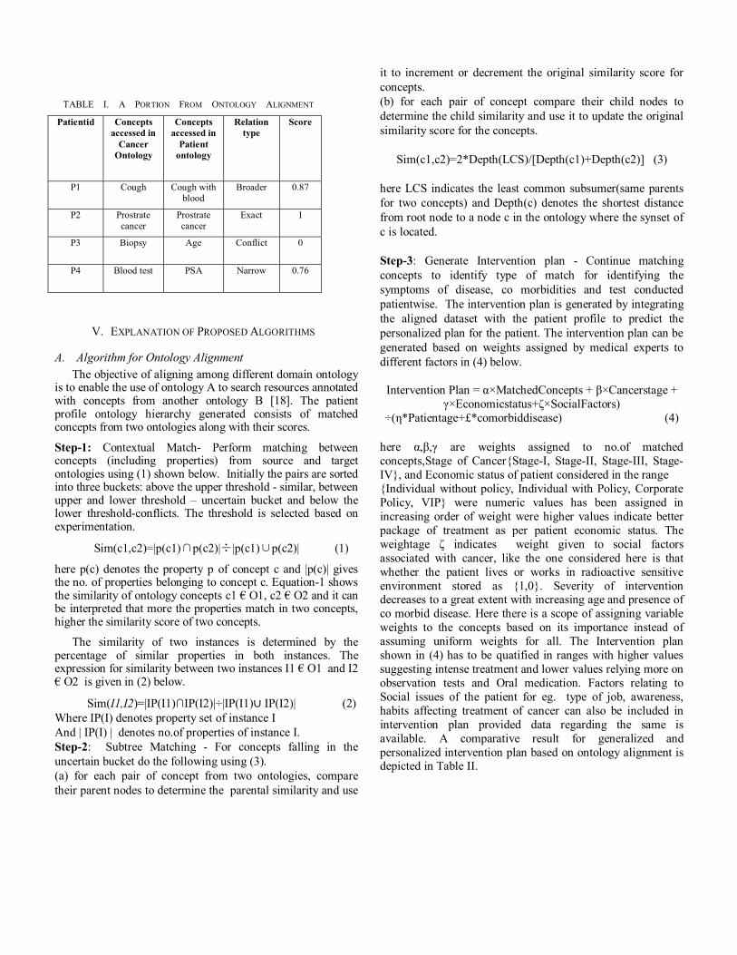
"
"
"
"
"
V. EXPLANATION OF PROPOSED ALGORITHMS
A. Algorithm for Ontology Alignment
The objective of aligning among different domain ontology is to enable the use of ontology A to search resources annotated with concepts from another ontology B [18]. The patient profile ontology hierarchy generated consists of matched concepts from two ontologies along with their scores.
Step-1: Contextual Match- Perform matching between concepts (including properties) from source and target ontologies using (1) shown below. Initially the pairs are sorted into three buckets: above the upper threshold - similar, between upper and lower threshold – uncertain bucket and below the lower threshold-conflicts. The threshold is selected based on experimentation.
Sim(c1,c2)=|p(c1) p(c2)| |p(c1) p(c2)| (1)
here p(c) denotes the property p of concept c and |p(c)| gives the no. of properties belonging to concept c. Equation-1 shows the similarity of ontology concepts c1 € O1, c2 € O2 and it can be interpreted that more the properties match in two concepts, higher the similarity score of two concepts.
The similarity of two instances is determined by the percentage of similar properties in both instances. The expression for similarity between two instances I1 € O1 and I2 € O2 is given in (2) below.
Sim(I1,I2+?KR*K3+yKR*K4+ÔKR*K3+姦 IP(I2)| (2)
Where IP(I) denotes property set of instance I
And | IP(I) | denotes no.of properties of instance I.
Step-2: Subtree Matching - For concepts falling in the
uncertain bucket do the following using (3).
(a) for each pair of concept from two ontologies, compare
their parent nodes to determine the parental similarity and use
it to increment or decrement the original similarity score for
concepts.
(b) for each pair of concept compare their child nodes to
determine the child similarity and use it to update the original
similarity score for the concepts.
Sim(c1,c2)=2*Depth(LCS)/[Depth(c1)+Depth(c2)] (3)
here LCS indicates the least common subsumer(same parents
for two concepts) and Depth(c) denotes the shortest distance
from root node to a node c in the ontology where the synset of
c is located.
Step-3: Generate Intervention plan - Continue matching
concepts to identify type of match for identifying the
symptoms of disease, co morbidities and test conducted
patientwise. The intervention plan is generated by integrating
the aligned dataset with the patient profile to predict the
personalized plan for the patient. The intervention plan can be
generated based on weights assigned by medical experts to
different factors in (4) below.
Kpvgtxgpvkqp"Rncp"?"g'OcvejgfEqpegrvu"-"く'Ecpegtuvcig"-"け'Geqpqokeuvcvwu-こ'UqekcnHcevqtu)
÷*さ,Rcvkgpvcig-,eqoqtdkffkugcug+ (4)
hgtg" g.く.け" ctg" ygkijvu" cuukipgf" vq" pq0qh" ocvejgf"concepts,Stage of Cancer{Stage-I, Stage-II, Stage-III, Stage-IV}, and Economic status of patient considered in the range{Individual without policy, Individual with Policy, Corporate Policy, VIP} were numeric values has been assigned in increasing order of weight were higher values indicate better package of treatment as per patient economic status. The ygkijvcig" こ" kpfkecvgu" " ygkijv" ikxgp" vq" uqekcn" hcevqtu"associated with cancer, like the one considered here is that whether the patient lives or works in radioactive sensitive environment stored as {1,0}. Severity of intervention decreases to a great extent with increasing age and presence of co morbid disease. Here there is a scope of assigning variable weights to the concepts based on its importance instead of assuming uniform weights for all. The Intervention plan shown in (4) has to be quatified in ranges with higher values suggesting intense treatment and lower values relying more on observation tests and Oral medication. Factors relating to Social issues of the patient for eg. type of job, awareness, habits affecting treatment of cancer can also be included in intervention plan provided data regarding the same is available. A comparative result for generalized and personalized intervention plan based on ontology alignment is depicted in Table II.
Patientid Concepts
accessed in
Cancer
Ontology
Concepts
accessed in
Patient
ontology
Relation
type
Score
P1 Cough Cough with blood
Broader 0.87
P2 Prostrate cancer
Prostrate cancer
Exact 1
P3 Biopsy Age Conflict 0
P4 Blood test PSA Narrow 0.76
TABLE I. A PORTION FROM ONTOLOGY ALIGNMENT

B.Pseudo code for Personal Recommendation based on
Ontology alignment
The patient and cancer ontologies are aligned to compute the matches in identifying the primary, co-occurring diseases, tests to be conducted. Based on these, medical professionals are provided smart recommendations while accepting any character for search. The pseudo code is provided below:
Step-1: Initializationalphabet1=array(alphabets);number1=array(prime numbers);datanum1=array(random numbers); data=array("PSA","bonescan","turp biopsy","CT scan, “Radiation","Uroflowmetry"); // concepts associated with lab test for prostrate cancer. String1 array stores the search made by usersearchitem=1;arrlength = count(alphabet1);
Step-2: Matching -If any character entered matches with stored alphabets then search multiplied with corresponding prime number.
for(i=0;i<strlen(string1);i++){ for(j=0;j<arrlength;j++)
{
if(string1[i]==alphabet1[j])
{
searchitem = searchitem * number1[j];
}
}
Step-3: Search Recommendation for user c=0;
for(i=0,j=0;i<count(datanum1);i++) {
if(datanum1[i]%searchitem==0)
{
possibleval[j]=data[i]; j++;c++;
} }
for(t=0;t<c;t++) {
Display possibleval[t]; }
}
VI. EXPERIMENT AND RESULTS
A. Data Set
The experimental data used in this work has been collected
from different cancer related websites which allows open
access and has been made publicly available for research
and study purposes [19-24]. The training data set
comprising of 2721 documents was used for the
representation of the cancer ontology indexing 204
concepts in the hierarchy. The testing was done selecting
fifty patients randomly who have different types and stages
of cancer. The software used for this work is jdk1.7, Html,
CSS, and Protégé
4.1.Results
Fig. 2. Comparison of F-measure for selected users
Patientid Primary disease
identified
Stage of cancer General
Intervention
plan for cancer
disease
Co occurent
disease based
on alignment
Age of patient
in yrs
Economic
status
Intervention
Plan
customized for
patient
1 Locally advanced
Prostate cancer
Stage-IIIChemotherapy
followed by observatory test
Fatty liver 57 Corporate policy Chemotherapy
followed by Radical
prostatectomy
2 Local Prostate cancer Stage-IIradiation therapy
followed by hormone therapy
Myocardial
ischemia
72 Individual policy Hormonal
therapy and observation
3 Non small cell Lung cancer
Stage-IIIChemotherapy
cycles with intermediate
medication and radiation.
Frequent Vomiting and
chest pain
21 Individual without policy
Chemotheray cycles with and
thoracentesis
4 Squamous
cell lung cancer
Stage-IIRadiation
Shortness of
breath and cough, fatigue
46 Corporate policy Lobectomy
followed by radiation
TABLE II. A COMPARISON OF GENERALIZED AND PERSONALIZED INTERVENTION PLAN GENERATED FROM ONTOLOGY ALIGNMENT
F-Measure

Fig. 3. Comparison of F-measure with varying threshold
B. Analysis of Experimental Results
The experimental evaluation was designed to retrieve the precision, recall and F-measure values and to study its variation with change in threshold [25]. A comparison of our ontology alignment based search has been evaluated using one, two and three keywords for top-n documents [26].The comparison of F-measure for intervention plans of five patients suffering from cancer is provided in Fig.2. The results confirmthat there is a sharp improvement in F-measure values in case of our Ontology Alignment model. The variation in F-measure values with changing threshold has been plotted in Fig.3. It has been observed that peak value for F-measure has been obtained at a threshold of 0.63. Fig.4 and Fig.5 provides the percentage in improvement in top Precision and Recall values for ontology alignment search results using one, two and three keywords. Both results show that there is a significant rise in precision and recall values using single keyword in our ontology alignment approach when compared with individual ontology search results. The improvement however decreases with the increase in keywords.
VII. SUMMARY AND FUTURE SCOPE
The work demonstrates use of Ontology alignment to generate intervention plans suitable for patients, integrating
the medical, personal and economic factors. The work uses contextual matching, and sub tree matching to accurately identify matches thus eliminating the ones not required for the patient. Smart recommendations are suggested to user based on searched domain which can be provided when the user inputs any search character for eg. tests required for lung cancer. The experimental results provided here are based on usage of randomly selected users, a few hundred queries, and a limited number of relevant documents. Future research in this area will consists of much larger scale of experiments and optimization parameters.
This heterogeneous ontology alignment can be applied to search among Digital libraries for plagiarism check of research papers submitted by authors. Another application of this work can be used by Software Development companies to archive the source code and components in an ontology framework which can be reused later for searching suitable codes and components applicable for specific projects.
REFERENCES
[1] Shady Shehata, Fakhri Karray, and Mohamed S. Kamel, An Efficient Concept-Based Mining Model for Enhancing Text Clustering, IEEE Transaction on Knowl. and Data Engineering, Vol. 22, No. 10, October 2010
[2] Lorena Otero-Cerdeira , Francisco J. Rodríguez-Martínez,,Alma Gómez- Rodríguez, Ontology matching: A literature review, Elsevier J. of Expert Systems with Applications, 42, 949–971, 2015.
[3] David Riano, Francis Real , Joan Albert Lopez-Vallverdu, Fabio ampana , Sara Ercolani, Patrizia Mecocci , Roberta Annicchiarico, Carlo Caltagirone, An ontology-based personalization of health-care knowledge to support clinical decisions for chronically ill patients, Elsevier J. of Biomedical Informatics, 45, 429–446, 2012.
[4] Scheuermann RH, Ceusters W, Smith B. Toward an ontological treatment of disease and diagnosis. In: Proceedings of the 2009 AMIA summit on translational bioinformatics, San Francisco (CA), p. 116–20, 2009.
[5] Healthcare Information exchange and interoperability www.citl.org/research/hiei.htm, Center for Information
Technology leadership, 2004. Last accessed on December 2015.
F-Measure
Top-nPrecision
%
Improvement
Documents
Fig. 4. Percentage of Improvement in Precision with Ontology Alignment Search using single and multiple words
Top-nRecall
%Improvement
Documents
Fig. 5. Percentage of Improvement in Recall with Ontology Alignment Search using single and multiple words
[6] Fang Liu, Clement Yu, Personalized Web Search for Improving Retrieval Effectiveness, IEEE Transactions on Knowl. and Data Engineering, Vol. 16, No. 1, January 2004.
[7] Rohana K.Rajapakse, Michael.Denham, Text retrieval with more realistic concept matching and reinforcement larning. Information Processing and Management.42(5),1260-127, September 2006.
[8] Ashraf, J., Khadeer Hussain, O., Khadeer Hussain, F.: AFramework for Measuring Ontology Usage on the Web.In: The Computer Journal. Oxford University Press, 2012.
[9] Miyoung Cho, Hanil Kim, and Pankoo Kim. A new method for ontology merging based on concept using Wordnet. In Advanced Communication Technology, 2006. ICACT 2006. The 8th International Conference, volume 3, pages 1573/1576, February 2006.
[10] M-Y.Chen, H-C.Chu, Y-M.Chen, Developing a semantic enable information retrieval mechanism. Expert Systems with Applications, 37:322-340, 2010.
[11] Juanzi Li, Jie Tang, Yi Li, and Qiong LuoRiMOM: A Dynamic Multistrategy Ontology Alignment Framework, IEEE Transactions on Knowledge and Data Engineering, Vol. 21, No. 8, August 2009
[12] Ontology Web Language, http://www.w3.org/TR/owl-features/ 2008. [Accessed on 20th December 2015]
[13] P. Lambrix and H. Tan, A Tool for Evaluating Ontology Alignment Strategies, J. of Data Semantics, Vol. 8, pp. 182-202, 2007.
[14] Schadd, F. C., & Roos, N. (2012). MaasMatch results for OAEI 2012. In P. Shvaiko, J. Euzenat, A. Kementsietsidis, M. Mao, N.
F. Noy, & H. Stuckenschmidt (Eds.), OM, CEUR-WS.org. (pp. 160–167).
[15] Paulheim, H., Hertling, S., & Ritze, D. (2013). Towards evaluating interactive ontology matching tools. Lecture notes in computer science LNCS, Vol. 7882, pp. 31–45.
[16] Brochhausen M, Spear AD, Cocos C, Weiler G, Martn L, Anguita A, et al. The ACGT master ontology and its applications – towards an ontology driven cancer research and management system. J Biomed Inform 2011;44(1): 8–25.
[17] http://protegewiki.stanford.edu[18] P. Shvaiko, J. Euzenat: Ontology matching: state of the art and
future challenges, IEEE Transactions on Knowledge and Data Engineering, 2013.
[19] http://www.cancer.org/research/index[20] http://www.cancercare.org/accessengagementreport [21] http://www.oncolink.org/resources[22] http://med.stanford.edu/cancer.html[23] http://www.ncbi.nlm.nih.gov/pubmed[24] http://www.cdc.gov/cancer/ [25] Yuan-chao Liu , Chong Wu, Ming Liu, Research of fast SOM
clustering for text information, Elsevier J. of Expert Systems with Applications 38 (2011) 9325– 9333.
[26] Paulo Cremonesi, Yehuda Koren, Roberto Turrin. Rerformance of recommender algorithms on top-n recommendation tasks. In Proc. of the fourth ACM conference on Recommender Systems, pp.39-46, New York, USA, 2010.

Comparison of Performance Metrics
of ModAODV with DSDV and AODV
Mrinal Kanti Deb Barma, Rajib Chowdhuri, Sudipta Roy
and Santanu Kumar Sen
Abstract In this paper, an adaptive routing in Mobile Adhoc Network (MANET)
is presented using special neighbors on different routes. The routing table of each
node is computed and stored in a metric. The path with the minimum cost is
selected as the primary routing path among all feasible paths. The Adhoc On—
Demand Distance Vector (AODV) Routing protocol is modified in such a way that
only the destination node will respond to a route request which greatly reduces the
transmission of control data packets in a network. The performance of modified
AODV is evaluated based on metrics such as throughput, packet delivery ratio, and
normalized routing overhead.
Keywords MANET � Throughput � Packet delivery ratio � Normalized routing
overhead
1 Introduction
The primary motivation toward the design and development of a Distance Vector
Routing (DVR)-based hybrid protocol for Mobile Adhoc Network (MANET) and
WSN kind of networks is mainly because of the simplicity and elegance of the
DVR algorithm, which is a traditional routing protocol based on Bellman Ford’s
M.K.D. Barma (&) � Rajib Chowdhuri
Department of Computer Science and Engineering, NIT Agartala, Jirania, Tripura, India
e-mail: [email protected]
Rajib Chowdhuri
e-mail: [email protected]
Sudipta Roy
Department of Computer Science and Engineering, Assam University, Silchar, India
e-mail: [email protected]
S.K. Sen
Department of Computer Science and Engineering, GNIT Kolkata, Kolkata, India
e-mail: [email protected]
© Springer Science+Business Media Singapore 2017
R. Singh and S. Choudhury (eds.), Proceeding of International Conference
on Intelligent Communication, Control and Devices, Advances in Intelligent
Systems and Computing 479, DOI 10.1007/978-981-10-1708-7_11
105

algorithm that later on got rejected mainly because of the Count-To Infinity
(CTI) problem of the DVRA. The second motivation forwards the development of
DVR-based routing algorithm for MANETs because of its neighbor exchange-
based routing technique, through which a route can view its whole world only
through a neighbor, and hence, need not to keep track of the whole network,
thereby reducing the burden of bandwidth and battery supply. Routing is the heart
of a network and optimality and reliability are the keen requirements for the success
of such routing protocol.
The goal of this paper is to modify the routing table of original Adhoc On—
Demand Distance Vector (AODV) protocol based on special neighbors of each
route to obtain a modified version of AODV protocol termed as ModAODV whose
performance is compared with that of AODV and DSDV in terms of throughput,
packet delivery ratio, and normalized routing overhead.
2 Comparison of ModAODV Protocol with DVR Protocol
The important disadvantages of DVR protocol is as follows:
Slow Convergence Problem: When there is an increase in the cost of any link or
there is a link failure between two neighboring nodes in a network or internetwork,
the algorithm, in the worst case, may require an excessive number of iterations to
converge or to terminate. The slow convergence phenomenon actually results from
the propagation of a bad news which implies a loss or increased distance of a route.
In the DVRA, the bad news travels slowly unlike the good news [1, 2].
Count to Infinity problem: DVR Algorithm suffers from the serious problem of CTI
[1, 3–5] which sometimes occurs following a link or router failure, due to unending
routing loops involving two or more routers. IP packets going round in loops are
ultimately dropped after expiry of the Time-to-Live (TTL), but they generate
considerable amount of unproductive traffic before being dropped.
Oscillation Problem: Because of the need to always use the shortest path, there may
be frequent switching of routes caused by even small increase or decrease in the
link costs. This frequent route switching gives rise to instability in routing and this
problem is known as the route oscillation problem [2].
3 Identification and Utilization of Special Neighbors
Distance Vector Routing Table (DVRT) is primarily used for identifying special
neighbors which are used in making ModAODV efficient and practical with fast
convergence and no CTI problem. The procedure of identification of special
neighbor and its method of utilization in case of both topological and traffic change
is based on the example network shown in Fig. 1.
106 M.K.D. Barma et al.
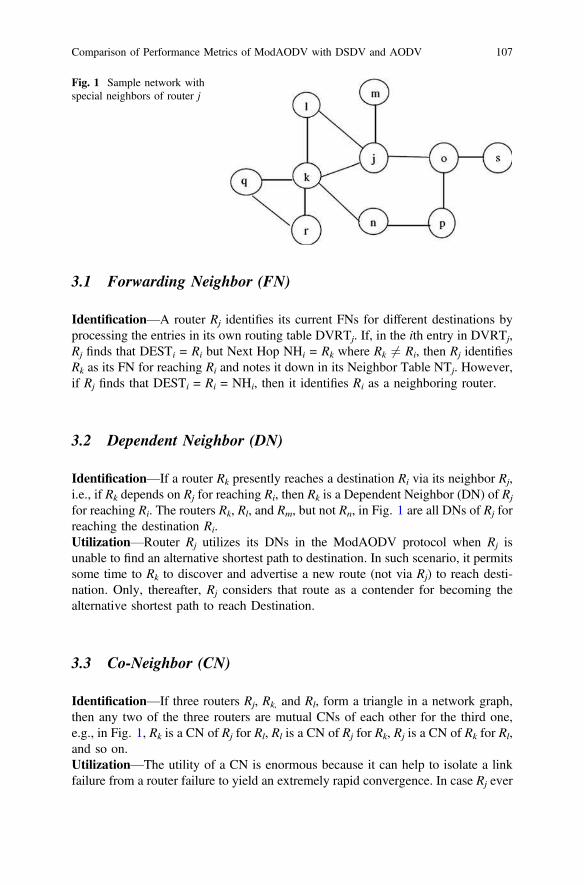
3.1 Forwarding Neighbor (FN)
Identification—A router Rj identifies its current FNs for different destinations by
processing the entries in its own routing table DVRTj. If, in the ith entry in DVRTj,
Rj finds that DESTi = Ri but Next Hop NHi = Rk where Rk 6¼ Ri, then Rj identifies
Rk as its FN for reaching Ri and notes it down in its Neighbor Table NTj. However,
if Rj finds that DESTi = Ri = NHi, then it identifies Ri as a neighboring router.
3.2 Dependent Neighbor (DN)
Identification—If a router Rk presently reaches a destination Ri via its neighbor Rj,
i.e., if Rk depends on Rj for reaching Ri, then Rk is a Dependent Neighbor (DN) of Rj
for reaching Ri. The routers Rk, Rl, and Rm, but not Rn, in Fig. 1 are all DNs of Rj for
reaching the destination Ri.
Utilization—Router Rj utilizes its DNs in the ModAODV protocol when Rj is
unable to find an alternative shortest path to destination. In such scenario, it permits
some time to Rk to discover and advertise a new route (not via Rj) to reach desti-
nation. Only, thereafter, Rj considers that route as a contender for becoming the
alternative shortest path to reach Destination.
3.3 Co-Neighbor (CN)
Identification—If three routers Rj, Rk, and Rl, form a triangle in a network graph,
then any two of the three routers are mutual CNs of each other for the third one,
e.g., in Fig. 1, Rk is a CN of Rj for Rl, Rl is a CN of Rj for Rk, Rj is a CN of Rk for Rl,
and so on.
Utilization—The utility of a CN is enormous because it can help to isolate a link
failure from a router failure to yield an extremely rapid convergence. In case Rj ever
Fig. 1 Sample network with
special neighbors of router j
Comparison of Performance Metrics of ModAODV with DSDV and AODV 107
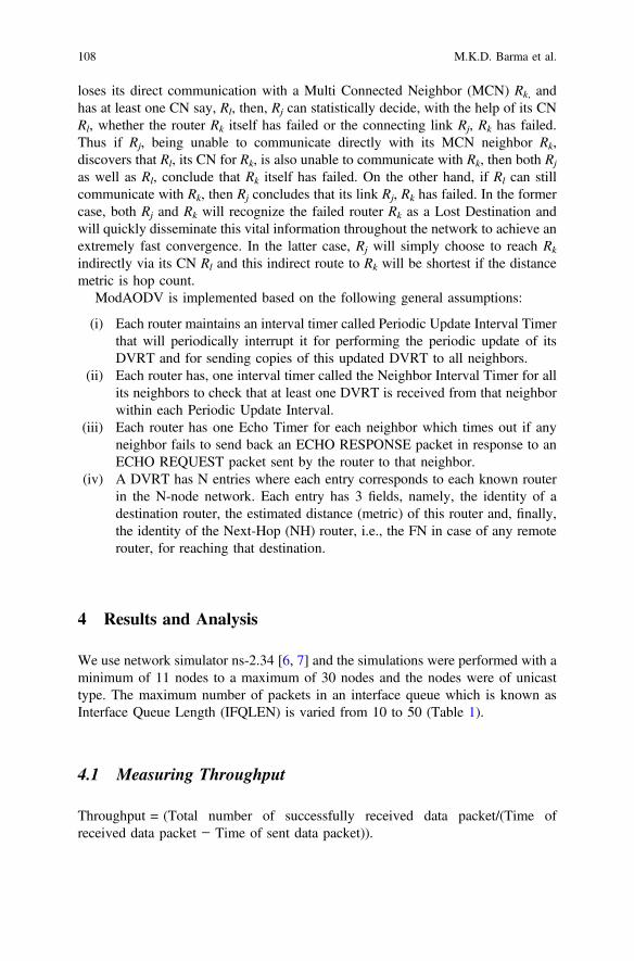
loses its direct communication with a Multi Connected Neighbor (MCN) Rk, and
has at least one CN say, Rl, then, Rj can statistically decide, with the help of its CN
Rl, whether the router Rk itself has failed or the connecting link Rj, Rk has failed.
Thus if Rj, being unable to communicate directly with its MCN neighbor Rk,
discovers that Rl, its CN for Rk, is also unable to communicate with Rk, then both Rj
as well as Rl, conclude that Rk itself has failed. On the other hand, if Rl can still
communicate with Rk, then Rj concludes that its link Rj, Rk has failed. In the former
case, both Rj and Rk will recognize the failed router Rk as a Lost Destination and
will quickly disseminate this vital information throughout the network to achieve an
extremely fast convergence. In the latter case, Rj will simply choose to reach Rk
indirectly via its CN Rl and this indirect route to Rk will be shortest if the distance
metric is hop count.
ModAODV is implemented based on the following general assumptions:
(i) Each router maintains an interval timer called Periodic Update Interval Timer
that will periodically interrupt it for performing the periodic update of its
DVRT and for sending copies of this updated DVRT to all neighbors.
(ii) Each router has, one interval timer called the Neighbor Interval Timer for all
its neighbors to check that at least one DVRT is received from that neighbor
within each Periodic Update Interval.
(iii) Each router has one Echo Timer for each neighbor which times out if any
neighbor fails to send back an ECHO RESPONSE packet in response to an
ECHO REQUEST packet sent by the router to that neighbor.
(iv) A DVRT has N entries where each entry corresponds to each known router
in the N-node network. Each entry has 3 fields, namely, the identity of a
destination router, the estimated distance (metric) of this router and, finally,
the identity of the Next-Hop (NH) router, i.e., the FN in case of any remote
router, for reaching that destination.
4 Results and Analysis
We use network simulator ns-2.34 [6, 7] and the simulations were performed with a
minimum of 11 nodes to a maximum of 30 nodes and the nodes were of unicast
type. The maximum number of packets in an interface queue which is known as
Interface Queue Length (IFQLEN) is varied from 10 to 50 (Table 1).
4.1 Measuring Throughput
Throughput = (Total number of successfully received data packet/(Time of
received data packet − Time of sent data packet)).
108 M.K.D. Barma et al.

In the first experiment, 5 (five) simulations were performed for each routing
protocol to obtain the values of throughput by varying the size of IFQLEN from 10
to 50.
Figure 2 shows the impact of increasing IFQLEN on throughput. The number of
nodes used in this experiment was 11. The maximum speed was Vm = 20.0 m/s and
pause time was 2.0 s and it is observed that throughput of modified AODV doubles
the throughput of original AODV and DSDV with increase in the number of
packets in the interface queue.
Table 1 Parameters used in
simulationParameter Value
Area of the network 500 m � 400 m
Simulation time 150 s
Packet size 512 Bytes
MAC type IEEE 802.11
Interface queue type Queue/DropTail/Priqueue
Mobility model Random waypoint
Traffic type CBR
Fig. 2 Measurement of
throughput with increase in
interface queue length
Comparison of Performance Metrics of ModAODV with DSDV and AODV 109
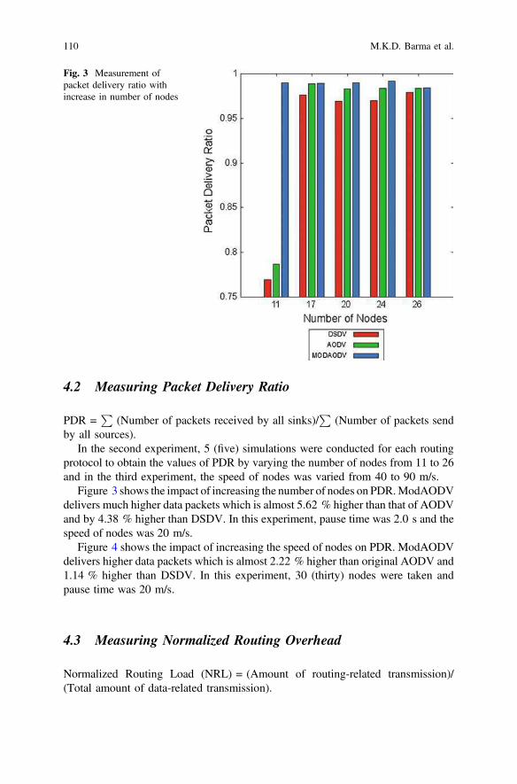
4.2 Measuring Packet Delivery Ratio
PDR =P
(Number of packets received by all sinks)/P
(Number of packets send
by all sources).
In the second experiment, 5 (five) simulations were conducted for each routing
protocol to obtain the values of PDR by varying the number of nodes from 11 to 26
and in the third experiment, the speed of nodes was varied from 40 to 90 m/s.
Figure 3 shows the impact of increasing the number of nodes on PDR.ModAODV
delivers much higher data packets which is almost 5.62 % higher than that of AODV
and by 4.38 % higher than DSDV. In this experiment, pause time was 2.0 s and the
speed of nodes was 20 m/s.
Figure 4 shows the impact of increasing the speed of nodes on PDR. ModAODV
delivers higher data packets which is almost 2.22 % higher than original AODV and
1.14 % higher than DSDV. In this experiment, 30 (thirty) nodes were taken and
pause time was 20 m/s.
4.3 Measuring Normalized Routing Overhead
Normalized Routing Load (NRL) = (Amount of routing-related transmission)/
(Total amount of data-related transmission).
Fig. 3 Measurement of
packet delivery ratio with
increase in number of nodes
110 M.K.D. Barma et al.

Fig. 4 Measurement of
packet delivery ratio with
increase in speed of nodes
Fig. 5 Measurement of
routing overhead with
increase in pause time
Comparison of Performance Metrics of ModAODV with DSDV and AODV 111

In this experiment, 5(five) simulations were performed for each routing protocol
to obtain the values of NRL by varying the pause time of nodes from 30 to 100 s.
Figure 5 shows the impact of increasing pause time of nodes on NRL which
clearly depicts that the routing overhead of ModAODV is much lower than that of
original AODV and DSDV except when pause time were 30 s and 40 s, overhead
of ModAODV is a bit higher compared to DSDV. In this experiment, 30 (thirty)
nodes were taken, speed of nodes was 20 m/s, and the size of IFQLEN was 50.
5 Conclusion
This paper compares the performance of a new routing protocol called ModAODV
with two foremost routing protocols DSDV and AODV using ns-2 simulations. The
results show that throughput of ModAODV doubles the throughput of original
AODV and DSDV with increase in IFQLEN. The impact of increasing the number
of nodes and speed of nodes depicts that ModAODV delivers much higher data
packets compared to AODV and DSDV. The impact of increasing the pause time of
nodes depicts that original AODV and DSDV has highest routing overhead com-
pared to ModAODV. Throughput decreases in case of DSDV since it needs to
advertise both periodic and event-driven updates but throughput of AODV remains
stable. Thus DSDV consumes more bandwidth compared to DSDV.
As our future work, we will try to include one more additional feature to this
ModAODV protocol like acknowledgement of data by the destination to the source.
References
1. A.S. Tenenbaum, “Computer Networks”, 5th Ed., Pearson Education Asea, 2010.
2. D.E. Comer, “Internetworking with TCP/IP”, 4th Ed., Pearson Education, Singapore, 2005.
3. S. K. Ray, S. K. Paira and S. K. Sen, “Modified Distance Vector Routing Avoids Counting -
To-Infinity Problem”, Proc. Intl. Conf. CODIS 2004, Kolkata, pp. 31–34, 2004.
4. S. K. Ray, J. Kumar, S. K. Sen and J. Nath, “Modified Distance Vector Routing Scheme for a
MANET”, Proc. Of the 13th National Conference on Communications (NCC), IIT Kanpur,
pp. 197–201, 2007.
5. A. Leon-Garcia and Indra Widjaja, “Communication Networks”, 2nd Ed., Tata McGraw-Hill,
2004.
6. K. Fall and K. Varadhan, “The NS Manual, (formerly ns Notes and Documentation)”,
The VINT Project: A Collaboration between Researchers at UC Berkeley, LBL, USC/ISI and
Xerox PARC, 2011.
7. Yan Li, “Mobile Ad Hoc Network Simulation: Analysis and Enhancements”, PhD thesis,
Heriot-Watt University, Edinburgh, UK, 2008.
112 M.K.D. Barma et al.

Mammogram Classification using Gray-Level Co-
occurrence Matrix for Diagnosis of Breast Cancer
Ranjit Biswas
Department of CSE
Assam University
Silchar, India
Abhijit Nath
Department of CSE
Assam University
Silchar, India
Sudipta Roy
Department of CSE
Assam University
Silchar, India
Abstract— Breast cancer is one of the most common forms of
cancer in women worldwide. Most cases of breast cancer can be
prevented through screening programs aimed at detecting
abnormal tissue. So, early detection and diagnosis is the best way
to cure breast cancer to decrease the mortality rate. Computer
Aided Diagnosis (CAD) system provides an alternative tool to the
radiologist for the screening and diagnosis of breast cancer. In
this paper, an automated CAD system is proposed to classify the
breast tissues as normal or abnormal. Artifacts are removed
using ROI extraction process and noise has been removed by the
2D median filter. Contrast-Limited Adaptive Histogram
Equalization (CLAHE) algorithm is used to improve the
appearance of the image. The texture features are extracted
using Gray Level Co-occurrence Matrix (GLCM) of the region of
interest (ROI) of a mammogram. The standard Mammographic
Image Analysis Society (MIAS) database images are considered
for the evaluation. K-Nearest Neighbor (KNN), Support Vector
Machine (SVM) and Artificial Neural Network (ANN) are used
as classifiers. For each classifier, the performance factor such as
sensitivity, specificity and accuracy are computed. It is observed
that the proposed scheme with 3NN classifier outperforms SVM
and ANN by giving 95% accuracy, 100% sensitivity and 90%
specificity to classify mammogram images as normal or
abnormal.
Keywords—Mammogram; ROI; GLCM; Confusion Matrix;
3NN classifier.
I. INTRODUCTION
Breast cancer grows in the breast cells usually in the lobules (glands which produce milk) and in the milk ducts (that carry milk to the nipple). In 2015, 40290 women death reported due to breast cancer [1]. The best way to identify the presence of breast cancer at an early stage is by interpreting mammogram images. Though mammography is an effective screening tool used by the radiologist for breast cancer detection at an early stage [2], however by visual interpretation it’s very difficult for the radiologist to classify the affected tissue whether it is cancerous or not. Sometimes, the mammography test can give negative results in the presence of tumor by not detecting the exact ROI where tumor is present. In such cases, further tests are required which can be expensive and time-consuming. Also, abnormal tissue region may also be missed in visual (manual) interpretation of a mammogram image. In recent years Computer Aided Detection (CAD) system are being used to solve the problem of interpretation of the mammogram image. (The mass or calcifications in the
breast tissue which may get unnoticed in visual interpretation by radiologists are easily and effectively being detected using CAD systems. The development and fine tuning of the CAD system has become more crucial for early and effective detection of abnormal tissues in the given digital mammogram image [3]. Thus, the main objective of CAD system is to increase diagnosis accuracy and enhancing the mammogram interpretation. Thus, CAD system can reduce the variability in judgments among radiologists by providing an accurate diagnosis of digital mammograms.
Rest of the paper is organized as follows: section 2 discusses about computer aided breast cancer detection systems; a new automated system is proposed and discussed in section 3; section 4 depicts the experimental results; conclusion and future work is discussed in section 5.
II. RELATED WORK
A CAD system was proposed in [4] for automatic detection and classification of breast cancer where noise and pectoral region removed from the breast using morphological operations and histogram based methods respectively. Using intuitionistic FCM based clustering, ROI is extracted and that ROI is transformed into four sub bands with the help of discrete wavelet transform (DWT). Wavelet energy features and 13 gray level co-occurrence features are computed form these sub bands. Then the self-adaptive resource allocation network (SRAN) classifier is used for classification. In 2013, tumor cut algorithm was proposed by Maanasa et al. for segmentation of mammogram image for detection of breast cancer [5]. Noise and artifact is removed using Gabor filter. Then from segmented image, geometrical and textural features are extracted. The optimal features are calculated using anova test calculator. With the help of optimal features, the mammogram image is classified into normal, benign and malignant using support vector machine (SVM) classifier.
S. Deepa et al. in [6] proposed a method for classification of mammogram image. According to abnormality given in the MIAS database, the ROI of size 256x256 is extracted. From the decomposed image, contourlet co-efficient is computed using contourlet transform and from that, co-efficient, co-occurrence matrix is generated. With the help of co-occurrence matrix, optimal features are selected using sequential floating forward selection (SFFS) algorithm. Probabilistic neural network is used for classification.
2016 International Conference on Micro-Electronics and Telecommunication Engineering
978-1-5090-3411-6/16 $31.00 © 2016 IEEE
DOI 10.1109/ICMETE.2016.85
163
2016 International Conference on Micro-Electronics and Telecommunication Engineering
978-1-5090-3411-6/16 $31.00 © 2016 IEEE
DOI 10.1109/ICMETE.2016.85
161

In 2014, Puneeth et al. [7] proposed a method for classification of mammogram image based on textural features, which is calculated using gray level co-occurrence matrix. K-Nearest Neighbors (KNN) classifier is used for classification.
In 2015, K. Vaidehi et al. [8] developed an intelligent system for retrieval of content-based mammogram image. In their proposed method, the features are calculated from the ROI. Using support vector machine image is classified and top 10 image is retrieved using KNN algorithm.
In 2015, Subashini et al. [9] developed a method where ROI is extracted from each mammogram image and from the ROI textural features are calculated using gray level co-occurrence matrix. Hybrid genetic algorithm-particle swarm optimization is used to select best features from the set of extracted features. With the help of optimal features, the image is classified using KNN algorithm.
In 2016, F Shirazi et al. in [10], presented a breast cancer detection system by combining mixed gravitational search algorithm (MGSA) and support vector machine (SVM). The authors used MIAS database and the features are extracted using gray level co-occurrence matrix (GLCM). In the experimental setup, the authors have use 70% of the dataset (out of 100 ROIs) as training dataset which includes normal and abnormal tissues. The rest of the 30% of the dataset is used as test objects and the results are computed upon that. By using only SVM with 24 features the performance was reported to be 86% whereas by the combination of MGSA – SVM with 12 features the performance was reported to be 93.1%.
III. PROPOSED SYSTEM
In this section, mammogram image classification system is proposed. The proposed system for classification of mammogram images is built based on GLCM by applying different classifiers. The system is divided into five stages to classify mammogram images. First step is the data set collection, second is ROI extraction process, third is the pre-processing steps which is again divided into two steps filtering and enhancement, fourth is the feature extraction from GLCM and last stage is classification. The architecture of the proposed system is shown in Fig. 1.
A. Dataset collection
In this experiment, the mammogram images were obtained from the MIAS [11] data set. MIAS is an organization of UK research groups interested in the understanding of mammograms and has generated the digital mammograms dataset for their research. It consists of 322 images of left and right breast from 161 patients, which contains normal and abnormal images, and abnormal images are again classified into benign and malignant. The dataset provides the details, about the location and radius of the abnormalities marked by expert radiologists. In the MIAS dataset, the mammogram originally was of the size of 1024×1024 pixels.
B. Region of Interest (ROI) Extraction process
Original mammogram images have different types of noises, artifacts in their background, pectoral muscles etc which are unwanted for feature extraction and classification. Hence a cropping operation has been applied on mammogram
Fig. 1: Architecture of Proposed Method
image to extract the ROIs which contains the abnormalities, apart from the unwanted portions of the image. MIAS database gives all the details about each mammogram image, viz., size in pixels, character of background tissue, class of abnormality, Xc and Yc coordinate value of centre of abnormality, ‘r’ radius of circle enclosing the abnormality by the radiologists. ROIs extraction performed by manual cropping operation considering the centre of the abnormal area as the centre of ROI and taking the approximate radius (in pixels) of a circle enclosing the abnormal area as shown in Fig. 2. For the extraction of normal ROI, the same cropping procedure has been performed on normal mammographic images with random selection of location. In this work, all the ROIs are resized in to 128 x 128 for uniformity. In this phase, the rectangular ROIs are extracted and the ROIs are free from the background information and artifacts, which is defined by equation (1) [12].
���� � ����� ���� �� �� ��� ��� (1)
C. Pre-Processing
A mammogram is an X-ray image of the breast. It may
contain noise and image quality may be poor. So
preprocessing step is mostly needed to make the image
suitable for classification. Thus, filtering technique is used to
Fig. 2: Cropping of ROI
MIAS Database
Region of Interest (ROI) Extraction
Noise Removal and Contrast
Enhancement
Features Extraction using GLCM
Mammogram ROIs Classification
Performance Evaluation
164162

remove noise and the enhancement technique is used to improve the image quality [13].
In this work, median filter is used as it preserves the information while removing noise. PSNR and MSE [14] values of the median filter are calculated and compared with two other filter techniques. Median filter performs better by giving highest PSNR value and lowest MSE value shown in table 1. Contrast of each pixel relative to its local neighborhood is adaptively enhanced during this process which is known as Contrast Limited Adaptive Histogram Equalization and to improve the appearance of the image contrast-limited adaptive histogram equalization (CLAHE) [15] is used here. Fig. 3 shows the result of contrast enhancement process.
D. Feature Extraction
In image processing, processing of large data is time consuming and less efficient for classification. For reducing time, the input data is transformed into reduced set of feature vector. This transformation process is called feature extraction process. This feature vector contains relevant information and is used as input vector for classification.
Features can be classified based on color, texture and shape. In this work, we are mainly concerned about texture features and for extraction of features; Gray Level Co-occurrence Matrix (GLCM) is used since it has been proven as a powerful tool for feature extraction [16]-[17]. In this work four textural features namely contrast, correlation, Energy, homogeneity are extracted with � � � and �= 00, 450, 950, 1350 and then take the average of these four direction.
(a) (b)
(c) (d)
Fig. 3: (a) De-noised image; (b) Histogram of (a); (c) Contrast enhanced image (d) Histogram of (c)
TABLE 1: PSNR AND MSE VALUE OF MAMMOGRAM SAMPLES
Image Averaging filter Wiener filter Median filter
PSNR MSE PSNR MSE PSNR MSE
Mdb01
5 3.52
28929.
74 26.63 141.23 37.28 12.17
Mdb14
5 3.28
30543.
91 26.64 140.84 38.86 8.46
E. Gray Level Co-occurrence Matrix (GLCM)
Grey level co-occurrence matrices (GLCM) are introduced in [18]-[19]. It explains the occurrence of certain grey levels in relation to other grey levels using statistical sampling. The process statement is reproduced as it is from [18]-[19] in the following paragraph.
Assume that an image to be analyzed is rectangular and has �� rows and �� columns. The gray level appearing at each
pixel is quantized to �� levels. Let, �� = {1,2,....,��} be the
rows, ��={1,2,....,��} be the columns and G={0,1,2,....��-1}
is the total number of gray levels quantized up to ��levels. The
set ��x�� is the set of pixels of the image ordered by their row-
column designations. Then, the image I can be represented as a function of co-occurrence matrix that assigns some gray level in ��x�� as I: ��x�� � �.
The texture-context information is specified by the matrix of relative frequencies � !�" with two neighbouring pixels
separated by distance�, one with gray level # and the other with gray level $ . Such matrices of gray-level co-occurrence frequencies are a function of the angular relationship � and distance d between the neighbouring pixels. By using a distance of one pixel and angles quantized to �%&intervals, four matrices of horizontal, first diagonal, vertical, and second diagonal (0, 45, 90 and 135 degrees) are used. Then, the un-normalized frequency in those four directions is defined by equation (2).
#� $� �� �� � '
()*)+
,� -�� .� /�01 ���2�����2� ��2���1 , . � �� 3- /3 � ���4�� , . � �� - / � ��4�� , . � �� - / � ���4�� 3, .3 � �� - / � ���4�� , . � �� - / � ���4�� , . � �� - / � ���� ,� -� � #�������� .� /� � $�
�� ��
Where # is the number of elements in the set, (k, l) the
coordinates with gray level i, (m, n) the coordinates with gray level j.
Consider #� $� be the #� $�th entry in a normalized GLCM. G is the number of gray levels range from 0 to ��-1. μ is the
mean value of p. 5�� 5�� 6�� 6� are the means and standard
deviations of � and � and presented in Equations (3), (4), (5)
and (6) respectively.
5� � 7 7 #8 #� $�9:;<"=&9:;<!=& (3)
5� � 7 7 $8 #� $�9:;<"=&9:;<!=& (4)
6� � 7 7 # 5��>9:;<"=&9:;<!=& 8 #� $� (5)
6� � 7 7 ?$ 5�@>9:;<"=&9:;<!=& 8 #� $� (6)
In this paper, four textural features namely contrast, correlation, Energy, homogeneity are extracted from mammogram ROIs using GLCM as formulated in [18]-[19]
Contrast:
A� � 7 />9:;<B=& C7 7 #� $�D� 39:"=<9:!=< # $3 � /� (7)
165163

Contrast is a relative measure of the intensity between a pixel and its neighbours over the whole image and is presented in equation (7). It is the quantity of local variation present in an image.
Correlation:
A� � 7 7 !"�E !�"�;FGFHIGIH
9:;<"=&9:;<!=& (8)
How a pixel is correlated to its neighbor over the whole image is known as correlation and is presented in equation (8). Feature values range from -1 to 1, these extremes indicating perfect negative and positive correlation respectively.
Energy:
AJ � 7 7 C #� $�D>9:;<"=&9:;<!=& (9)
Energy also known as uniformity or angular second
moment (ASM). Energy measure the sum of squared elements in the GLCM as presented in equation (9). Basically the property of energy is provide how uniform the texture image. The range of energy is [0 1], where Energy is 1 for a constant image.
Homogeneity:
A� � 7 7 E !�"�<K !;"�L
9:;<"=&9:;<!=& (10)
It measures the closeness of the distribution of the elements
in the GLCM to the GLCM diagonal and is defined in equation (10). The range of homogeneity is [0 1], where homogeneity is 1 for a diagonal GLCM. It is high when local gray level is uniform and inverse GLCM is high.
F. Classification
Last step of the proposed method is the classification of the mammogram image into normal or abnormal. Here, the classification is done mainly with the help KNN algorithm and compared with SVM and ANN classifiers.
KNN is a supervised learning that has been used in many applications in the field of data mining and pattern recognition. This classifier computes the distance from the unlabeled data to every training data point and selects the best k-neighbor with the shortest distance. This classifier implementation is very simple since there is no need of explicit training step. The input to the classifier is the k-closest training samples and the output is the class name or a class membership. The output is decided by majority vote of its neighbours, where the input is being assigned to the class most frequent among its k-nearest neighbours. When k is considered as 1, then the input is just allocated to that class.
In this present study 1NN and 3NN are considered and Euclidean distance is used for calculating the distance between the new samples and training samples. Different k values give different results.
IV. EXPERIMENTAL RESULT AND DISCUSSION
To carry out the research, 208 mammogram images are considered out of which 188 images are used as a training set
TABLE 2: GLCM FEATURES VALUE FOR TEST DATASET
Image Contrast Correlation Energy Homogeneity
mdb190 0.1606 0.9073 0.2173 0.9225
mdb193 0.1313 0.8719 0.3492 0.9366
mdb199 0.1493 0.8560 0.2947 0.9282
mdb204 0.1768 0.9293 0.1929 0.9134
mdb208 0.1354 0.9616 0.2595 0.9347
mdb209 0.1510 0.9518 0.1814 0.9267
mdb212 0.1527 0.9180 0.2150 0.9255
mdb214 0.1868 0.9414 0.1504 0.9083
mdb219 0.1919 0.9470 0.1537 0.9060
mdb226 0.1868 0.9507 0.1382 0.9101
mdb234 0.2052 0.9331 0.1580 0.9000
mdb245 0.1767 0.8382 0.2810 0.9150
mdb246 0.0784 0.8818 0.5188 0.9639
mdb252 0.1616 0.9620 0.1402 0.9206
mdb257 0.1307 0.8268 0.3763 0.9362
mdb264 0.1496 0.9113 0.2591 0.9281
mdb272 0.1812 0.8195 0.2968 0.9122
mdb282 0.1501 0.7991 0.3470 0.9270
mdb302 0.1571 0.8367 0.3081 0.9236
mdb304 0.1476 0.9099 0.3128 0.9288
and 20 (10 normal and 10 abnormal) images are taken as testing set. From the de-noised and contrast enhanced ROI based mammogram images, the four texture features are calculated with the help of gray level co-occurrence matrix. These features are used as an input to the KNN classifier for training and testing.
To evaluate the performance of the proposed system the following parameters are used which is defined by the equations (11),(12) and (13)[20].
Accuracy =MNKMO
P x 100% (11)
Specificity =MO
MOKQN x 100% (12)
Sensitivity = MN
MNKQO x 100% (13)
Where, True positive (TP) = the mammogram image predicted with abnormal when actually the mammogram image is abnormal.
True negative (TN) = the mammogram image predicted with normal when the mammogram image actually normal.
False positive (FP) = the mammogram image predicted with abnormal when the mammogram image is normal.
166164

False negative (FN) = the mammogram image predicted with normal when the mammogram image is abnormal.
Accuracy defines the overall correctness of the classifier, specificity defines true negative rate and sensitivity defines true positive rate. The higher values of both sensitivity and specificity show better performance of the system. Tables 3, 4, 5 and 6 show the classification result using 1NN, 3NN, SVM and ANN respectively with the help of confusion matrix. The overall performance of the proposed method is shown in table 7. The performance of the four classifiers are compared and represented graphically in fig. 4.
From the graphical representation of fig. 4, it is revealed that 3NN classifier outperforms other three in terms of accuracy and specificity whereas in terms of sensitivity 3NN outperforms SVM and ANN clearly and equals with 1NN. Thus, 3NN can be considered as a more efficient classifier for the classification of the mammogram ROIs images than 1NN, SVM and ANN.
TABLE 3: CONFUSION MATRIX FOR 1NN
Target class Predicted class
Normal Abnormal
Normal 7(TN) 3(FP)
Abnormal 0(FN) 10(TP)
TABLE 4: CONFUSION MATRIX FOR 3NN
Target class Predicted class
Normal Abnormal
Normal 10(TN) 0(FP)
Abnormal 1(FN) 9(TP)
TABLE 5: CONFUSION MATRIX FOR SVM
Target class Predicted class
Normal Abnormal
Normal 6(TN) 4(FP)
Abnormal 3(FN) 7(TP)
TABLE 6: CONFUSION MATRIX FOR ANN
Target class Predicted class
Normal Abnormal
Normal 7(TN) 3(FP)
Abnormal 2 (FN) 8(TP)
TABLE 7: CLASSIFICATION RESULS
Methods Accuracy % Sensitivity % Specificity %
1NN 85 100 70
3NN 95 100 90
SVM 65 70 60
ANN 75 80 70
Fig. 4: Performance comparison of 1NN, 3NN, SVM, ANN classifiers
V. CONCLUSION AND FUTURE WORK
The CAD system is developed and presented here for the classification of mammogram into normal and abnormal breast tissues with the aim to support the radiologists in visual diagnosis. The experimental results show that 3NN gives the maximum accuracy rate for normal and abnormal classification (96%) compared to other classifiers.
The present work can be extended to the whole MIAS database with 322 mammogram images or other mammogram databases too. In future, more number of other statistical movement features may be considered with proper feature selection technique and accuracy may be improved further. A new mammogram database can be created by collecting mammogram images from different clinics and hospitals and this proposed method may be tested on that database.
REFERENCES
[1] American Cancer Society, “Breast cancer facts & figures 2015-2016,” Atlanta, American Cancer Society, Inc. 2015.
[2] L. Tabar, P.Dean, “Mammography and breast cancer: the new era,” International Journal of Gynecology and Obstetrics, vol. 82, Issue 3, September 2003, pp. 319-326.
[3] H. Cheng, X. Shi, R. Min, L. Hu, X. Cai, H. Du, “Approaches for automated detection and classification of masses in mammograms,” Pattern recognition, vol. 39, 2006, pp. 646-668.
[4] S. Shanthi, and V. Murali Bhaskaran,“Computer aided system for detection and classification of breast cancer,” International Journal of Information Technology, Control and Automation,vol. 2, no. 4, October 2012, pp. 87-98.
[5] Maanasa N A S, V Gowri, “Segmentation of mammogram using tumor-cut algorithm,” International Journal of Engineering and Innovative Technology, vol. 2, Issue 10, April 2013, pp. 172-175.
[6] S. Deepa, V. Subbiah Bharathi, “Textural feature extraction and classification of mammogram images using CCCM and PNN,” IOSR Journal of Computer Engineering, vol. 10, Issue 6, 2013, pp. 07-13.
[7] Puneeth L., Krishna A.N. “Classification of mammograms using texture features,” International Journal of Innovative Research & Development, vol. 3, Issue 7, July 2014, pp. 373-377.
[8] K. Vaidehi, T. S. Subashini, “An intelligent content based image retrieval system for mammogram image analysis,” Journal of Engineering Science and Technology, vol. 10, 2015, pp.1453 – 1464.
[9] Subashini Sundaravinayagam, Bhavani Sankari. S, “Detection and classification of masses in mammograms using a hybrid GA-PSO-KNN approach,” International Journal of Advanced Research Trends in Engineering and Technology, vol. 2, May 2015.
[10] F. Shirazi, E. Rashedi, “Detection of cancer tumors in mammography images using support vector machine and mixed gravitational search algorithm,” In proceedings of IEEE 1st Conference on Swarm
0
20
40
60
80
100
120
1NN 3NN SVM ANN
Va
lue
()%
Classification methods
Accuracy
Sensitivity
Specificity
167165
Intelligence and Evolutionary Computation, Bam, March 2016, pp. 98-101, doi:10.1109/CSIEC.2016.7482133.
[11] S. A. J Suckling, D Betal, N Cerneaz, D R Dance, S-L Kok, J Parker, I Ricketts, J Savage, E Stamatakis and P Taylor, “The mammographic image analysis society digital mammogram databaseeExerpta medica,” International Congress Series 1069, 1994, pp. 375-378.
[12] R. N. Panda, M. A. Baig, B. K. Panigrahi, M. R. Patro “Efficient CAD system based on GLCM & derived feature for diagnosing breast cancer,” International Journal of Computer Science and Information Technologies, vol. 6, 2015, pp. 3323-3327.
[13] Mister Khan, Sumit Kataria and Smriti, “Mammography based breast cancer detection using different classifiers,” National Conference on Emerging Trends in Electronics & Communication, vol. 1, No. 2, July 2015.
[14] K. Malathi, R. Nedunchelian, “Comparision of various noises and filters for fundus Images using pre-processing techniques,” International Journal of Pharma and Bio Sciences, vol. 5, july 2014, pp. 499-508.
[15] K. Zuiderveld, “Contrast Limited Adaptive Histogram Equalization,” Academic Press Inc, 1994.
[16] Pradeep N, Girish H, Karibasappa K, “Segmentation and feature extraction of tumors from digital mammograms,” Computer Engineering and Intelligent Systems, vol 3, No.4, 2012.
[17] Biswajit Pathak, Debajyoti Barooah, “Texture analysis based on the graylevel co-occurence matrix considering possible orientations,” International Journal of Advanced Research in Electrical, Electronics and Instrumentation Engineering, Vol. 2, September 2013.
[18] Robert M. Haralick, K. Shanmugam, and ITS’HAK Dinstein, “Textural features for image classification,” IEEE Transaction on system, man and cybernetics, vol.SMC-3, No.6, November 1973, pp. 610-621.
[19] L.K. Soh, and C. Tsatsoulis, “Texture analysis of sar sea ice imagery using grey level co-occurrence matrices,” IEEE Transactions on Geoscience and Remote Sensing, vol.37, no. 2, March 1999, pp. 780-795.
[20] R. Nithya B. Santhi, “Classification of normal and abnormal patterns in digital mammograms for diagnosis of breast cancer,” International Journal of Computer Applications, vol. 28, August 2011, pp. 21-25.
168166
Web Service Discovery based on IR Models:
A Review
Arnab PaulDepartment of Comp. Sc. & Engg.
Assam University, SilcharAssam, India
Sudipta RoyDepartment of Comp. Sc. & Engg.
Assam University, SilcharAssam, India
Monowar HussainDepartment of Comp. Sc. & Engg.
Assam University, SilcharAssam, India
Abstract—Web service discovery is one of the major research thrust areas in the field of computing environment. From last decade, a good number of researchers are contributing their thoughts in finding the best available service from a pool of services that can satisfy the user’s requirement. Different researchers have adopted different methodologies and ideas to visualize their noble thoughts in the field of web service discovery. Information retrieval methods are one of them. Utilization of IR methods in service discovery approaches makes the discovery process efficient. In this paper, we focus on those service discovery approaches which employ information retrieval methods for the purpose of automatic discovery. This paper provides a survey of how these approaches differ from each other while discovering a service.
Keywords: Web Service Discovery; Information Retrieval etc.
I. INTRODUCTION
Web services are loosely coupled, distributed and independent application components that can be published, found and used on the web[1]. W3C defines web service as: “A Web service is a software system designed to support interoperable machine-to-machine interaction over a network. It has an interface described in a machine-processable format (specifically WSDL). Other systems interact with the Web service in a manner prescribed by its description using SOAP messages, typically conveyed using HTTP with an XML serialization in conjunction with other Web-related standards”[2].
Web services runs on the technologies called WSDL (Web Service Description Language), UDDI (Universal Description, Discovery and Integration) and SOAP (Simple Object Access Protocol). WSDL[3] describes services a set of network endpoints. WSDL document provides the functionalities of a service in XML format. UDDI[4] is the universally accepted XML based standard service repository in which the services in WSDL format can be published. Services in Service Oriented Architecture (SOA) can communicate with each other through SOAP[5]. SOAP is a lightweight XML based
protocol for exchange of information in a decentralized, distributed environment.
Web service discovery is one of the most popular domains in SOA. The fundamental concept is that web service providers publish their services in the service repository and web service consumers use those services; web service discovery is the process of finding the most appropriate service from the repository that satisfies the consumers’ need.
Automatic discovery of web services without human intervene is a popular research area for many researchers. Researchers have suggested many methods for the automatic discovery of web services. Our paper focuses on those discovery processes which utilize information retrieval methods for the purpose of automatic discovery. The paper is organized as follows: section II provides overview of web service discovery mechanism; section III discusses some of the information retrieval methods; section IV deals with various approaches taken by many authors for web service discovery; section V concludes the study.
II. WEB SERVICE DISCOVERY
If a web service consumer wishes to avail a service but is unaware of the providers of the service, then the consumer must initiate the ‘discovery’ process. Discovery is "the act of locating a machine-processable description of a Web service that may have been previously unknown and that meets certain functional criteria"[1].
The web service providers publish their web service descriptions along with the associated functional descriptions of the services in the form WSLD in the service repository. In order to use some services available in the service repository, the service consumers need to provide the service requirements based on the associated functional descriptions. Based on the consumer’s service criteria, the discovery unit finds the appropriate service from the service repository that fulfills the specified criteria and returns the associated service

Figure 1.Web Service Discovery process
description to the consumer. If the discovery unit returns more than one services for single query, then the consumer has to select one of them based on some additional criteria. Both service provider and consumer must agree on the service description and the semantics of the interaction. And then, the provider and consumer communicates by exchanging the SOAP messages[1].
III. INFORMATION RETRIEVAL MODELS
Information retrieval is the study of finding unstructured documents from a large collection of documents with respect to a given query. IR can be broadly classified in two categories: semantic and statistical. Semantic technique extends retrieval capability by adding both syntactical and semantic analysis. Semantic analysis utilizes the contextual meaning of the user query to produce more relevant result. In statistical IR techniques, the documents which match the user query most closely are retrieved based on some statistical measures[6].
Boolean, vector space and probabilistic methods are the widely used statistical approaches in IR. The documents and the queries are often broken into words, generally referred to as terms. These terms need to undergo a number of preprocessing techniques before using them in any statistical measures [6].
Boolean IR is the oldest and simplest Information Retrieval model. In Boolean information retrieval system, any query can be expressed in terms of Boolean expression. The terms in the query are combined with the operators and, or, and not [7]. The result of a Boolean query is either true or false. A document is either relevant or irrelevant w.r.t. a query depending on whether the document satisfies the query or not[6]. For a query, this model retrieves that document for which it finds the exact match. Partial matches are not retrieved and also there is no ranking mechanism[10].
In Vector Space Model[8], each document is represented as vector of terms.
dj = {w1j , w2j , . . . , wtj}
where, t represents the total number of terms in the document collection. If a term is present in the document, then the weight for the term in the document vector is non zero. The query is also represented as a vector of terms in Vector Space Model. There are two different techniques for computing the term weights of the terms present in the document vector and query vector: term-frequency (tf) and inverse document frequency (idf). The next step is to measure the similarity between the query vector and each of the document vectors. The similarity is generally measured using the cosine similarity[9]. The documents whose similarity values are greater than the threshold value are retrieved as a set of relevant documents. In vector Space Model, the term weights are not binary; partial matching and ranking of documents are possible. The order of appearance of the terms in the document does not coincide when represented as vector space which is one of the limitations of this model. Another limitation is that this model does not capture the semantics of the query and document[10].
Probabilistic IR model retrieves documents based on the probability of the document relevant to the query. The Probabilistic Ranking Principle[11] (PRP) is as follows:
“If a reference retrieval system's response to each request is a
ranking of the documents in the collection in order of
decreasing probability of relevance to the user who submitted
the request, where the probabilities are estimated as
accurately as possible on the basis of whatever data have
been made available to the system for this purpose, the overall
effectiveness of the system to its user will be the best that is
obtainable on the basis of that data”.
For a document vector d and query vector q, the documents are ranked according to their probability of relevance w.r.t. the query: P(R = 1|d, q), where R is the indicator random variable which is either 1 or 0 based on whether d is relevant or nor relevant with respect to the query respectively.
The Binary Independence Model[7] is a probabilistic IR model which employs some basic assumptions to make feasible estimate of the probability similarity between the document and the query. One assumption is that both documents and query are represented as binary term incidence vectors. Another assumption ‘independence’ means that the terms in documents are independent of each other having no association between them. The probability P(R|d, q) that a document is relevant is modeled based on the probability of
Service Repository
Find
BindService
ProviderService
Provider
Publish

relevance of the term incidence vectors P(R|捲, 圏). Then, using Bayes rule, we get 鶏岫迎 = な|捲, 圏岻 = 牒岫掴|眺 退 怠,槌屎 岻牒岫眺 退 怠|槌屎 岻牒岫掴,槌屎 岻鶏岫迎 = ど|捲, 圏岻 = 牒岫掴|眺 退 待,槌屎 岻牒岫眺 退 待|槌屎 岻牒岫掴,槌屎 岻where 鶏岫捲|迎 = な, 圏岻 and 鶏岫捲|迎 = ど, 圏岻 represent the probability of retrieving relevant or irrelevant documents
respectively with document representation as 捲. For a particular query, a document will be either relevant or irrelevant, which implies: 鶏岫迎 = な|捲, 圏岻 + 鶏岫迎 = ど|捲, 圏岻 = な
IV. LITERATURE SURVEY
In this paper[12], they propose an algorithm based on the concept of singular value decomposition (SVD) of linear algebra to locate the similar services for a service request. For the purpose of retrieving similar services, they first collect keywords from the service descriptions of web services available in UDDI registry. These words are passed through a preprocessing stage which involves the elimination of stop words and then obtaining stemmed words. In this way, they build a collection of unique words for all the services present in the UDDI. All the words in the collection are assigned weight which is the value of inverse document frequency of the corresponding word. In the next step, vectors for all services are created where the value of each vector element for a particular service is calculated based on the weight of each word multiplied by its binary occurrence in that service. A service matrix is constructed considering all these vectors and then the singular value decomposition method of linear algebra is applied on this service matrix to find the relationship between services, define threshold for retrieving similar services and filter out the irrelevant services. To find similar services for a given service, they apply the concept of cosine similarity measurement. They present a comparison table between keyword matching technique and their SVD based proposed model which shows better result for their model.
In this paper[13], they propose a method for the analysis and discovery of Web services. They combine one of the information retrieval methods and the existing standards that describe the web services for the purpose of web service discovery. For a service request, their search engine finds the similar service/s from a collection of web services based on the information like functionalities, descriptions etc. of the
services. The distributed search engine employs the concept of vector space model of information retrieval system to discover the analogous service for a specific service request. The first step in their model deals with the extraction of keywords like endpoint URLs, types and their attribute names, message names, service names and XML comments from web services that are available in the WSDL file repository. Using these extracted keywords, a vector space is created where each dimension is represented by a term. Each document (WSDL file) is represented by a vector within this vector space. Vector elements of each vector are assigned normalized term weights calculated based on the term frequency and inverse document frequency of the term. They also extend their model to work with distributed vector space. The query processor extracts keywords from the given query string and also creates the query vector. The cosine similarity value is calculated between the query vector and each document vector present in the term space. Documents are then sorted based on their similarity rating. Their model works fine in distributed environment.
In this paper[14], they propose a flexible service discovery method to discover useful services. Textual elements of the service request are compared against textual elements of all available services in the repository to discover similar services and to rank them according to their similarity. To carry out this task, they use vector space model of information retrieval system. Next, a structure matching algorithm is projected on this ranked list of services to refine and evaluate the quality of the service set. For this purpose, they develop a heuristic, domain-specific tree-edit distance algorithm. WSDL specifications describing the web services based on XML syntax are hierarchical in nature. Therefore, the tree-edit distance algorithm can calculate the similarity between two tree structures as because minimum node modifications required to match them. Comparing two web services is based on comparison of service operations which, in turn, is based on comparison of service messages which again is based on comparing the data-types of the WSDL specifications. The algorithm matches the data-types, messages and operations of the WSDL specifications respectively. Each of these three steps results in individual matrix that evaluates the similarity score of all pair-wise combinations of source and target data-
types/ messages/ operations. The final similarity score is the maximum score calculated as the sum of matching scores of all individual operation pairs. Their report includes experiments on service discovery with IR methods only, with structure matching only and with IR and structure matching combined. For service discovery with IR methods only, they report a precision of 51% at 95% recall on average; with

structure matching only, they report a precision of 20% at 72% recall on average. The retrieval system with IR and structure matching combined achieves a precision of 61.5% at 90% recall with an increase in precision by 10.5% and drop in recall by 5% as compared to retrieval technique with IR method only.
In this paper[15], they propose a web-service search method to discover similar service operations given a natural language description of the desired service. Their work is almost similar to that of Wang & Stroulia[14], but they focus on semantic similarity rather than structural similarity. For a given service description, they first obtain a candidate set of service operations by using TF and IDF techniques of Information retrieval System. Web service data-types can be primitive or complex. Primitive data-types do not contain semantic information. Primitive data-types are converted to complex data-types by replacing them with their corresponding parameters to contain semantic meaning. XML schema is modeled as a tree of labeled nodes. The labeling is done as tag node and constraint node. Constraint node is further subdivided as sequence node, union node and multiplicity node. They apply bottom-up-transformation algorithm of time complexity O(n) in which they propose three transformation rules to transform all three constraint nodes to tag nodes. The service operation matching is done with the help of schema tree matching. On the candidate operations set, they use tree edit distance approach of schema matching algorithm to calculate the similarity among the operations. To measure tree edit distance between two schema trees, they introduce a new cost model to compute the cost of each edit operation which is based on weights and semantic connection of nodes. After identifying similarity of web service operations, the candidate set of service operations is clustered using agglomeration algorithm. For each cluster, operation with minimum cost will be output as search result. Since operations are associated with scores, they rank the search result based on scores of operations.
Aabhas V. Paliwal et al.[16] present an approach for web service discovery combining the concepts of ontology linking and Latent Semantic Indexing (LSI) in combination. Ontology linking is achieved by mapping domain ontology against upper merged and mid-level ontologies. LSI determines the relationship between query terms and the available documents to capture the domain semantics. After preparing the service request vector using domain ontology linking concept and service description vector from the selected WSDL documents using the LSI classifier, both the vectors are put together
utilizing the cosine similarity technique to determine the similarity and to discover the relevant web services. After preprocessing of the service request, it is enhanced by associating the related upper concepts utilizing the upper ontology which helps in web service categorization. From these categorized service collections, the service descriptions are extracted and parsed to form the term-document matrix. The SVD transformation applied on term-document matrix produces reduced dimension vector for each term and each document which helps to determine the appropriate web service. Because of the categorization of services, their experimental results produce a better result.
To avoid huge number of retrieved services w.r.t. a keyword and the inability of the keywords to express semantic concepts, Jiangang Ma et al[17] propose a clustering semantic algorithm to semantically discover the web services. First they prepare a working dataset by using a clustering semantic algorithm. For a particular query, the dataset is prepared based on the relevant web services whose contents are compatible with the query. They employ K-means clustering algorithm to eliminate the irrelevant services w.r.t. a query. They use the Vector Space Model to prepare the service transaction matrix for the services in the working dataset. The working dataset is then grouped into a number of semantically related clusters by employing the concept of Probabilistic Latent Semantic Analysis approach (PLSA). This PLSA technique is used to capture the semantic concepts of the terms of the query and also the descriptions of the services which helps to determine the semantic similarity between the service and the query within the related cluster. The PLSA utilizes the Bayesian network model and an intermediate layer called hidden factor variable to associate the keywords to its corresponding documents. For each and every service of the service dataset, the PLSA computes the probability w.r.t. each latent hidden variable. Then it determines the maximum probability for each service and puts the service in the semantically related cluster. By comparing the similarity between the query and related clusters, a set of relevant services are retrieved for the query.
Ricardo Sotolongo et al.[18] propose an approach that employs the Vector Space Model of IR in combination with Vector Space Model enhanced with lexical database WordNet to efficiently discover the web services. WordNet is utilized to capture the semantics of the WSDL elements that assist in deriving the accurate similarity. They also use Linear Discriminant Function of pattern classification technique to devise the relative similarity between the term and term’s synonyms and calculate the optimized weights of the terms

TABLE I. COMPARISON TABLE
Authors Method(s) Used
Similarity
Measur-
ement
Advantage Disadvantage
Distributed
or
Centralized
Semantic
Capability
Atul Sajjanhar, Jingyu Hou, and Yanchun Zhang[12]
Singular Value Decomposition
Cosine value
Is not restricted by the tModel used by a web service during publishing
1. Poor term weighting scheme
2. No semantic issue
Centralized No
Christian Platzer and Schahram Dustdar[13]
Vector Space Model
Cosine similarity value
Works fine in distributed environment
Does not deal with semantic search
Both No
Yiqiao Wang and Eleni Stroulia[14]
Vector Space Model and Structure Matching Algorithm (Tree-Edit Distance Algorithm)
Inspired bysignature-matching methods for componentretrieval
Structural matchingmay be invalid when two web-service operations havemany similar substructures on data types
Centralized No
Yanan Hao and Yanchun Zhang[15]
Tree-Edit Distance Algorithm, Bottom-up-transformationalgorithm
Results in better precision and recall value than keyword searchingmethod, structure matching methodand Woogle
Deals in very less semantic information
Centralized Partial
Aabhas V. Paliwal, Nabil R. Adam andChristof Bornhövd[16]
Ontology Linking and Latent Semantic Indexing
Cosine similarity
Better result because of categorization of services
Cost of computing LSI in SVD transformation is high
Centralized Yes
Jiangang Ma, Yanchun Zhang and Jing He[17]
ClusteringProbabilistic Semantic Approach (CPLSA)
Cosine similarity and PLSA
Produces good result for using cluster based probabilistic approach over traditional keyword based search
Will function poorly for high dimensional data
Centralized Yes
Ricardo Sotolongo, Carlos Kobashikawa, Fangyan Dong, and Kaoru Hirota[18]
Vector Space Model enhanced with WordNet
Inner product between weights of terms of WSDL and query vectors
Calculation of an optimal weight using batchperceptron algorithm of linear discriminant functions
Cost of computation is high because of calculation of relative frequency, global and relative importance, local and global similarity for both original and enhanced vectors
Decentraliz-ed
Yes

using batch perceptron algorithm. For both original vector and vector enhanced with WordNet, they calculated (i) the relative frequency of each word in each WSDL document, (ii) global importance of each word in all WSDL collection, (iii) relative importance of each word in each WSDL document. The same procedures are used for the query vector also. The local similarities between the WSDL and the query for both original and the enhanced vectors are calculated as the inner product of the relative importance of words in WSDL and relative importance of words in query. Finally, the global similarly between the WSDL and the query is calculated based on the local similarities in case of both original and enhanced vectors. They compared their algorithm with four other IR based WS discover algorithms and found that their algorithm is showing an improvement of 0.6% to 1.9% in precision and 0.7% to 3.1% in recall for the top 15 web services.
V. CONCLUSION
Finding the efficient service that satisfies the user’s need is a most challenging task in the field of web service discovery mechanisms under SOA. Various techniques have been developed to answer this issue. We concentrated on the information retrieval techniques related service discovery approaches in this paper. We discussed some of the basic information retrieval methods in this paper. We also discussed the advantages and disadvantages of the approaches used for service discovery. Most of the authors have used cosine similarity to address the issue of similarity measurement. Some approaches are centralized in their nature while some others are distributed. Also some approaches focus on semantic capability to make the discovery process an efficient one. We also agree that discovery units should address the semantic capability precisely in order to find the most appropriate service.
REFERENCES
[1] Papazoglou, M. P., Georgakopoulos, D., “Service-oriented computing”, Communications of the ACM, Vol. 46, No. 10, 2003, pp. 25–28.
[2] (2004, February) Web Services Architecture [Online]. https://www.w3.org/TR/2004/NOTE-ws-arch-20040211/
[3] (2001, March) Web Services Description Language (WSDL) 1.1 [Online]. https://www.w3.org/TR/wsdl
[4] (2004, October) UDDI Spec Technical Committee Draft [Online]. http://www.uddi.org/pubs/uddi_v3.htm
[5] (2000, May) Simple Object Access Protocol (SOAP) 1.1 [Online]. https://www.w3.org/TR/soap/
[6] Ed Greengrass, “Information Retrieval: A Survey”, Available online at: www.csee.umbc.edu/csee/research/cadip/.../IR.report.120600.book.pdf
[7] Christopher D. Manning, Hinrich Schütze, and Prabhakar Raghavan, “Introduction to Information Retrieval”, © Cambridge University Press 2008,ISBN-13 978-0-511-41405-3
[8] G. Salton, A. Wong and C. S. Yang, “A vector space model for automatic indexing”, Communications of the ACM, v.18 n.11, p.613-620, Nov. 1975
[9] Sidorov, Grigori; Gelbukh, Alexander; Gómez-Adorno, Helena; Pinto, David. "Soft Similarity and Soft Cosine Measure: Similarity of Features in Vector Space Model". Computación y Sistemas 18 (3): 491–504. doi:10.13053/CyS-18-3-2043
[10] Joydip Datta, “Ranking in Information Retrieval”, M. Tech Dissertation, Dept. of CSE, IITB, India, 2010.
[11] S.E. Robertson. The Probability Ranking Principle in IR. Journal of Documentation, 33(4):294-304, 1977. doi: 10.1108/eb026647. http://www.emeraldinsight.com/10.1108/eb026647.
[12] Atul Sajjanhar, Jingyu Hou, and Yanchun Zhang, “Algorithm for Web Services Matching”, Lecture Notes in Computer Science, vol. 3007, pp. 665-670, © 2004, Springer-Verlag.
[13] Christian Platzer and Schahram Dustdar, “A Vector Space Search Engine for Web Services”, in Proceedings of the Third European Conference on Web
Services (ECOWS’05), Washington, DC, USA, 2005, pp. 62 – 70, © IEEE Computer Society, doi: 10.1109/ECOWS.2005.5
[14] Yiqiao Wang and Eleni Stroulia, “Flexible Interface Matching for Web-Service Discovery”, In Proceedings of the Fourth International Conference on Web Information Systems Engineering (WISE’03), 2003 © IEEE Computer Society, pp. 147 – 156, doi: 10.1109/WISE.2003.1254478
[15] Yanan Hao and Yanchun Zhang, “Web Services Discovery Based on Schema Matching”, In Proceedings Thirtieth Australasian Computer Science Conference (ACSC2007), Ballarat, Australia, Conferences in Research and Practice in Information Technology (CRPIT), Vol. 62. Gillian Dobbie, Ed., pp. 107 – 113, ©2007, Australian Computer Society, Inc.
[16] Aabhas V. Paliwal, Nabil R. Adam, Christof Bornhovd, “Web Service Discovery: Adding Semantics through Service Request Expansion and Latent Semantic Indexing”, In International Conference on Services Computing (SCC 2007), IEEEXplore, 2007.
[17] Jiangang Ma , Yanchun Zhang and Jing He, “Efficiently finding web services using a clustering semantic approach”, In Proceedings of the 2008
International Workshop on Context Enabled Source and Service Selection, Integration and Adaptation: organized with the 17th International World Wide Web Conference (WWW 2008), p.1-8, April 22-22, 2008, Beijing, China, doi:10.1145/1361482.1361487
[18] Ricardo Sotolongo, Carlos Kobashikawa, Fangyan Dong, and Kaoru Hirota, “Algorithm forWeb Service Discovery Based on Information Retrieval UsingWordNet and Linear Discriminant Functions”, Journal of Advanced Computational Intelligence and Intelligent Informatics, Vol.12 No.2, pp: 182-189, 2008.
978-1-5090-0612-0/16/$31.00 ©2016 IEEE
Image Segmentation Using Spatial Fuzzy C Means Clustering and Grey Wolf Optimizer
1Th. Ibungomacha Singh, 2Romesh Laishram
Manipur Institute of Technology Takyelpat, Manipur, India
[email protected], [email protected]
Sudipta Roy
Assam University Silchar, Assam, India [email protected]
Abstract— Image segmentation is one research area of image
processing which has many applications in practice. In this paper
we have undertaken image segmentation problem using spatial
fuzzy c means (SFCM) clustering which is an unsupervised
classification scheme. A good segmentation result is desirable for
classification problem especially in medical image classification.
Therefore SFCM clustering result is further optimized using a
new colony based optimization algorithm called the grey wolf
optimizer (GWO). Experiments were conducted for segmentation
of magnetic resonance imaging (MRI) images. Comparative
results are presented to show the effectiveness of incorporating
GWO in to SFCM for image segmentation problem. Performance
parameters are given in terms of clustering validity functions.
Keywords—image segmentation; SFCM; GWO; MRI
I. INTRODUCTION
Image segmentation has been one of the thrust areas in the field of digital image processing for many years. Image segmentation [1] can be defined as the grouping of pixels into regions satisfying some criteria such that the region of interest (ROI) is well separated for detail analysis. Research in this area has revisited again particularly in medical image segmentation problem. Recently Computer aided diagnosis (CAD) is one of the main focus area of medical image processing.
Image segmentation problem can be thought of as a classification problem thereby making it suitable for the use of many machine learning based classification algorithms. Any classification algorithm can be broadly categorized into two types viz. supervised learning and unsupervised learning. One important algorithm in unsupervised learning is the fuzzy c- means (FCM) [2] clustering algorithm. In this paper we have considered the segmentation problem as a clustering in which different regions in the image are taken as clusters. The classical FCM algorithm has been used in image segmentation problem for many years and many versions of FCM were proposed and studied. In this work we have used one such variants of FCM which is called spatial-FCM (SFCM) proposed in [3]. It has proved to perform better than FCM by considering the spatial constraints in the design of FCM.
The clustering algorithm is further optimized by incorporating swarm based optimization algorithm. A swarm algorithm works on the principle of cooperation in solving a
problem. There are numerous swarm algorithm which were mostly natured inspired. We have consider one recently proposed swarm algorithm called grey wolf optimizer (GWO) [4] which is a model of the hunting mechanism of grey wolves.
By combing SFCM and GWO we proposed a new image segmentation method which we called SFCMGWO. The purpose of the optimization algorithm is to further optimize the cluster centers obtained from SFCM. In medical image segmentation problem accuracy is the main criteria determining the usefulness of the algorithm rather the complexity of the algorithm. The proposed combined algorithm is tested in MRI medical image segmentation problem.
The remainder of the paper is organized as follows. Section II highlights the related works done earlier in the field of MRI image segmentation. In Section III, a brief analysis of GWO and the algorithm is presented. SFCM and SFCMGWO are explained in Section IV. Experimental analysis of the proposed algorithm on MRI image segmentation is detailed in section V and finally conclusion is drawn in Section VI.
II. RELATED WORKS
In this section some of the recent works in the field of MRI image segmentation are highlighted. A comprehensive review of the human brain MRI segmentation is given in the article [5]. MRI segmentation based on pattern recognition algorithms are presented by the authors in [6] and FCM for brain MRI segmentation is studied in [7]. A new variant of FCM i.e. SFCM is introduced by Keh-Shih Chaung et el. [3]. The spatial information is incorporated in SFCM has shown certain advantages over FCM in obtaining more homogenous regions in the segmented image. The algorithm is also less sensitive to noise. SFCM is further integrated with level set methods for automated medical segmentation as proposed in the research work [8]. A hybrid of different variants of FCM is proposed in [9], where the combination of different FCM variants is studied for brain tumor segmentation. The scheme obtained improvements by achieving computationally fast and good accuracy in segmentation results.
The optimization of FCM by incorporating nature inspired optimization algorithm is proposed [10] by using the popular genetic algorithm (GA). Since then this fusion algorithm is quite popular and extensively studied for segmentation

2016 IEEE International Conference on Computational Intelligence and Computing Research
problems in the works carried out by the authors in [11]-[13].The combination of other swam intelligence like particle swarm optimization (PSO) and artificial bee colony (ABC) with FCM for medical image segmentation can be found in the literatures [14-16].
In this paper a combination of SFCM and GWO i.e. (SFCMGWO) is proposed for undertaking the problem of image segmentation in medical images and especially MRI images.
III. SPATIAL FCM (SFCM)
A brief description of clustering based on the most popular FCM algorithm and its variant SFCM are presented.
The FCM algorithm assigns pixels to different cluster based on the fuzzy membership function of the pixels to belong in a particular cluster. It is an optimization algorithm that minimizes an objective function iteratively.
Let us consider an image arranged in a one dimensional matrix as X=[x1,x2,.........xN], where xi represents pixel intensity value or feature value and N is the total pixels in the image. The aim of FCM is to partition the pixels in to c
clusters. In the standard FCM the cost function is defined in (1).
2
1 1
. ij
N
j
c
i
mij vxuJ −=
= =
(1)
The membership value of pixel xj to belong in ith cluster is denoted as uij, vi is the cluster center and m is a parameter that controls the partition result. The membership values and the updation of cluster centers are done according to equation (2) and (3) respectively.
( )=
−
−
−
=
c
k
m
kj
ij
ij
vx
vx
u
1
1
2
1 (2)
=
==
N
j
mij
N
j
jmij
i
u
xu
v
1
1 (3)
The information of neighborhood pixels is exploited in SFCM. It is highly possible that the neighborhood pixels possesses same feature value and belong to the same cluster. This concept is not considered in the standard FCM. The spatial information is exploited in SFCM by defining a spatial function [3] as in (4).
=)( jxNBk
ikij uh
ε
(4)
Where NB(xj) is a window define on the image centered on the pixel xj. The size of the window can 3x3 or 5x5 but in this we have considered only 5x5 window. The spatial hij is defined as the probability that a pixel xj belongs to the ith cluster. A higher value indicates that the most of the neighborhood pixels of a center pixel under consideration belongs to that cluster. The standard FCM is modified by incorporating the spatial function in the membership function. The modified membership function is defined in (5) which is reproduced from [3].
=
=c
k
qkj
pkj
qij
pij
ij
hu
huu
1
(5)
where p and q are parameters that decides the impact of the original membership function and the spatial function respectively in the calculation of new membership functions. The notation used for spatial FCM with parameters p and q is SFCMp,q. When p=1 and q=0 SFCM degenerates to conventional FCM.
The spatial FCM operates in two phase iteration. In the first phase the membership values are determined using the conventional FCM. This membership values are utilized in the calculation of the spatial function. In the second phase new membership function is calculated using (2). After the condition for convergence is achieved the iteration is over. The threshold for the convergence can be set when there is no change between two cluster centers in last two successive iterations. After the iteration is completed defuzzification process is initiated in which a pixel whose membership function is maximal is assigned to that cluster.
IV. GREY WOLF OPTIMIZER (GWO)
The Meta-heuristic based optimization algorithm has been successfully applied in many engineering and other related problems. Over the last many years research effort in this direction saw developing many popular algorithms like Genetic algorithm (GA), particle swarm optimization (PSO), artificial bee colony (ABC) etc. In this paper we focus on a newly proposed meta-heuristic algorithm called Grey Wolf Optimizer (GWO) proposed in [4]. It is inspired by the behaviour of grey wolves (Canis lupus) which maintains a hierarchy among them and follows unique steps in hunting. To mathematically model the hierarchical structure, four types of grey wolves are defined such as alpha (α), beta (β), delta (δ) and omega (ω). The leader is the alpha and most of the decisions are taken by alpha.The alpha is also called dominant wolf. Beta grey wolves are the second group in the hierarchy.They support alpha in decision making and act as subordinates of alpha. The lowest in the hierarchy is the omega. They always have to submit to all other dominant woves. If a wolf is not alpha, beta and omega they are called
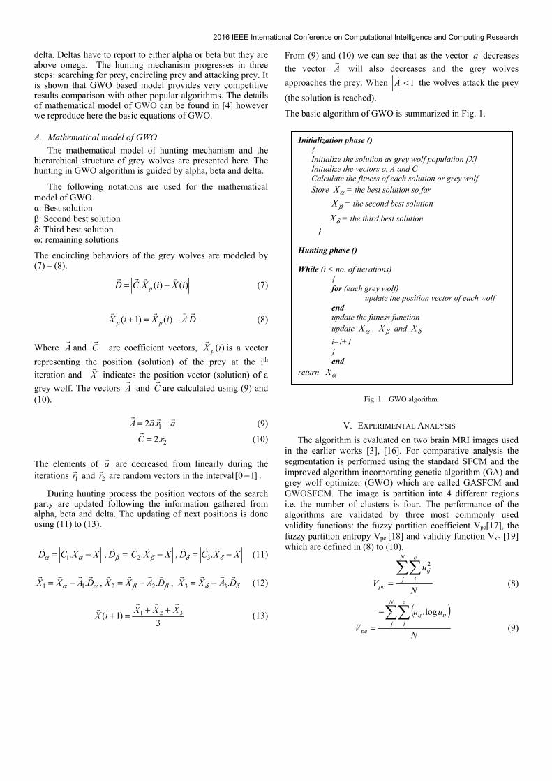
2016 IEEE International Conference on Computational Intelligence and Computing Research
delta. Deltas have to report to either alpha or beta but they are above omega. The hunting mechanism progresses in three steps: searching for prey, encircling prey and attacking prey. It is shown that GWO based model provides very competitive results comparison with other popular algorithms. The details of mathematical model of GWO can be found in [4] however we reproduce here the basic equations of GWO.
A. Mathematical model of GWO
The mathematical model of hunting mechanism and the hierarchical structure of grey wolves are presented here. The hunting in GWO algorithm is guided by alpha, beta and delta.
The following notations are used for the mathematical model of GWO. α: Best solution β: Second best solution δ: Third best solution ω: remaining solutions
The encircling behaviors of the grey wolves are modeled by (7) – (8).
)()(. iXiXCD p
−= (7)
DAiXiX pp
.)()1( −=+ (8)
Where A
and C
are coefficient vectors, )(iX p
is a vector
representing the position (solution) of the prey at the ith
iteration and X
indicates the position vector (solution) of a
grey wolf. The vectors A
and C
are calculated using (9) and
(10).
araA
−= 1.2 (9)
2.2 rC
= (10)
The elements of a
are decreased from linearly during the
iterations 1r
and 2r
are random vectors in the interval ]10[ − .
During hunting process the position vectors of the search party are updated following the information gathered from alpha, beta and delta. The updating of next positions is done using (11) to (13).
XXCD
−= αα .1 , XXCD
−= ββ .2 , XXCD
−= δδ .3 (11)
αα DAXX
.11 −= , ββ DAXX
.22 −= , δδ DAXX
.33 −= (12)
3
)1( 321 XXXiX
++=+ (13)
From (9) and (10) we can see that as the vector a
decreases
the vector A
will also decreases and the grey wolves
approaches the prey. When 1<A
the wolves attack the prey
(the solution is reached).
The basic algorithm of GWO is summarized in Fig. 1.
Fig. 1. GWO algorithm.
V. EXPERIMENTAL ANALYSIS
The algorithm is evaluated on two brain MRI images used in the earlier works [3], [16]. For comparative analysis the segmentation is performed using the standard SFCM and the improved algorithm incorporating genetic algorithm (GA) and grey wolf optimizer (GWO) which are called GASFCM and GWOSFCM. The image is partition into 4 different regions i.e. the number of clusters is four. The performance of the algorithms are validated by three most commonly used validity functions: the fuzzy partition coefficient Vpc[17], the fuzzy partition entropy Vpe [18] and validity function Vxb [19] which are defined in (8) to (10).
N
u
V
N
j
c
i
ij
pc
=
2
(8)
( )
N
uu
V
N
j
c
i
ijij
pe
−
=
log.
(9)
Initialization phase ()
{
Initialize the solution as grey wolf population [X]
Initialize the vectors a, A and C
Calculate the fitness of each solution or grey wolf
Store αX = the best solution so far
βX = the second best solution
δX = the third best solution
}
Hunting phase ()
While (i < no. of iterations)
{
for (each grey wolf)
update the position vector of each wolf
end
update the fitness function
update αX , βX and δX
i=i+1
}
end
return αX

2016 IEEE International Conference on Computational Intelligence and Computing Research
}){.(min
2
2
ikki
N
j
c
i
ijij
xbvvN
vxu
V−
−−
=
≠
(10)
The fuzzy partition validity functions Vpc and Vpe indicate
the level of fuzziness for better performance. The clustering result is good when Vpc is maximal or Vpe is minimal. The validity function Vxb gives the connection between fuzzy partition and feature property of the image. The inclusion feature makes Vxb more important than Vpc and Vpe. The clustering result achieved is best when Vxb is minimum.
The segmentation results are shown in Fig.2 and Fig.3 for two different sample images respectively. The result showed that the performance of GWO based SFCM is better than the standard SFCM and GASFCM. The results are further validated the validity functions as given tin table 1. GWOSFCM has the least value of Vxb and this value has more significance than the other two validity functions. GWOSFCM has also less utilization compared to GASFCM. This indicates that the GWO based algorithms are computationally fast yet very effective. The convergence of the fitness function of GASFCM and GWOSFCM are shown in Fig 4. The GWO has faster convergence than GA has attains minimum value of the cost function.
Fig. 2. (a) Original MRI image 1(b) SFCM segmentted image (c) GASFCM segmented image (d) GWOSFCM segmented image.
Fig. 3. (a) Original MRI image 1(b) SFCM segmentted image (c) GASFCM segmented image (d) GWOSFCM segmented image.
TABLE I. CLUSTER VALIDITY FUNCTIONS AND TIME COST FOR
DEIFFRENT ALGORITHMS
Test
images
Algorithm Validity functions CPU
Time
(sec)Vpc Vpe Vxb (x10-3)
Image1
SFCM 0.90 0.074 1.3 4
GASFCM 0.82 0.057 0.97 31
GWOSFCM 0.88 0.046 0.72 29
Image 2
SFCM 0.92 0.063 1.7 5
GASFCM 0.85 0.044 1.2 54
GWOSFCM 0.85 0.042 0.91 52
(a) (b) (c) (d)
(a) (b) (c) (d)

2016 IEEE International Conference on Computational Intelligence and Computing Research
Fig. 4. Convergence of fitness function of GASFCM and GWOSFCM.
VI. CONCLUSION
The challenging problem of image segmentation is undertaken in this paper by considering segmentation as clustering problem. A recently proposed optimization algorithm i.e. grey wolf optimizer (GWO) is incorporated in the standard spatial FCM (SFCM). Experimental results on brain MRI images clearly show that GWO based SFCM has better segmentation results compared to SFCM and GASFCM. It can be concluded from this study that GWO is computationally fast and a very effective algorithm. Further the algorithm can be tested on other images and the performance in a corrupted image can also be considered for robustness.
REFERENCES
[1] Rafael C. Gonzalez, Richard E. Woods, “Digital Image Processing, Pearson Education”, Second Edition, ISBN 81-7758-168-6, 2005.
[2] Bezdek, J. C., “Pattern Recognition with Fuzzy Objective Function Algorithms”, Plenum, NY, 1981.
[3] Keh-Shih Chuang, Hong-Long Tzeng, Sharon Chen, Jay Wu, Tzong-Jer Chen, “Fuzzy c-means clustering with spatial information for image segmentation”, Computerized Medical Imaging and Graphics, Volume 30, Issue 1, January 2006, pp. 9-15.
[4] Seyedali Mirjalili, Seyed Mohammad Mirjalili, Andrew Lewis, “Grey Wolf Optimizer”, Advances in Engineering Software, Volume 69, March 2014, pp. 46-61
[5] C. Bezdek, L.O. Hall, L. P. Clarke, “Review of MR image segmentation techniques using pattern recognition”, Med. Phys., vol. 20, No. 4, pp.1033-1048, 1993.
[6] Ivana Despotović, Bart Goossens, and Wilfried Philips, “MRI Segmentation of the Human Brain: Challenges, Methods, and Applications”, Computational and Mathematical Methods in Medicine, 2015.
[7] Balafar M. A., “Fuzzy c -means based brain MRI segmentation algorithms”, Artificial intelligence review, Springer Netherlands,2012.
[8] Bing Nan Li, Chee Kong Chui, Stephen Chang, S.H. Ong, “Integrating spatial fuzzy clustering with level set methods for automated medical image segmentation”, Computers in Biology and Medicine, Volume 41, Issue 1, January 2011, pp. 1-10.
[9] Eman Abdel-Maksoud, Mohammed Elmogy, Rashid Al-Awadi, “Brain tumor segmentation based on a hybrid clustering technique”, Egyptian Informatics Journal, Volume 16, Issue 1, March 2015, pp.71-81.
[10] Yingjie Wang, “Fuzzy Clustering Analysis Using Genetic Algorithm”, and ICIC International @ 2008 ISSN 1881-803 X, pp: 331—337.
[11] Y. Gao, S. Wang and S. Liu. Automatic Clustering Based on GA-FCM for Pattern Recognition, “Computational Intelligence and Design”, ISCID '09. Second International Symposium on, Changsha, 2009, pp. 146-149.
[12] A.Halder, S.Pramanik, A.Kar, “Dynamic Image Segmentation using Fuzzy C-Means based Genetic Algorithm”, International Journal of Computer Applications (0975 – 88 87) Volume 28– No.6, August 2011, pp.: 15 – 20.
[13] Romesh Laishram, W.Kanan Kumar Singh, N.Ajit Kumar, Robindro.K, S.Jimriff, “MRI Brain Edge Detection Using GAFCM Segmentation and Canny Algorithm”, International Journal of Advances in Electronics Engineering, Volume 2: Issue 3 ISSN 2278 - 215X, 2012.
[14] Laishram, R.; Kumar, W.K.; Gupta, A.; Prakash, K.V., “A Novel MRI Brain Edge Detection Using PSOFCM Segmentation and Canny Algorithm”, IEEE International Conference on Electronic Systems, Signal Processing and Computing Technologies (ICESC), 2014, vol., no., pp.398-401.
[15] Kamalam Balasubramani, Dr. Karnan Marcus, “Artificial Bee Colony Algorithm to improve brain MR image segmentation”, International Journal on Computer Science and Engineering (IJCSE), 2013.
[16] Thiyam Ibungomacha Singh, Romesh Laishram, Sudipta Roy, “Medical Image Segmentation Using Fuzzy C Means Clustering with Optimization using Artificial Bee Colony Algorithm”, Advanced Research in Electrical and Electronic Engineering, p-ISSN: 2349-5804; e-ISSN: 2349-5812 Volume 2, Issue 12 July-September (2015) pp. 35-40.
[17] Bezdek JC., “Cluster validity with fuzzy sets”, J. Cybern. 1974; 3:58-73.
[18] Bezdek JC., “Mathematical models for systematic and taxonomy”, proceedings of 8th international conference on numerical taxonomy, San Francisco; 1975, pp. 143-66.
[19] Xie Xl, Beni GA., “Validity measure for fuzzy clustering”, IEEE Trans on Pattern Anal. Mach. Intell. 1991;3:841-6.

Denoising of MRI Images Using Curvelet
Transform
Ranjit Biswas, Debraj Purkayastha and Sudipta Roy
Abstract Most of the medical images are usually affected by different types of
noises during acquisition, storage, and transmission. These images need to be free
from noise for better diagnosis, decision, and results. Thus, denoising technique
plays an important role in medical image analysis. This paper presents a method of
noise removal for brain magnetic resonance imaging (MRI) image using curvelet
transform thresholding technique combined with the Wiener filter and compares the
result with the curvelet and wavelet-based denoising techniques. To assess the
quality of denoised image, the values of peak signal-to-noise ratio (PSNR), mean
square error (MSE), and structural similarity index measure (SSIM) are considered.
The experimental results show that curvelet denoising method depicts better result
than wavelet denoising method, but the combined method of curvelet with Wiener
filtering technique is more effective than the wavelet- and curvelet-based denoising
method in terms of PSNR, MSE, and SSIM.
Keywords Wiener filter � Wavelet transform � Curvelet transform � Denoising
1 Introduction
Medical images are having an important role for diagnosis of diseases. These
images are obtained from various methods such as MRI, CT, and X-ray imaging.
Nowadays, these images are captured using digitized systems. During the
R. Biswas (&)
Department of Information Technology, Ramkrishna Mahavidyalaya, Kailashahar,
Tripura 799277, India
e-mail: [email protected]
D. Purkayastha � S. RoyDepartment of Computer Science & Engineering, Assam University, Silchar 788011, India
e-mail: [email protected]
S. Roy
e-mail: [email protected]
© Springer Nature Singapore Pte Ltd. 2018
A. Konkani et al. (eds.), Advances in Systems, Control and Automation,
Lecture Notes in Electrical Engineering 442, https://doi.org/10.1007/978-981-10-4762-6_55
575

acquisition process, the images may be corrupted by different types of noise and it
is very important to remove the noise to get better interpretation. Removal of noise
from digital images is a big challenge for the researchers. Huang et al. [1] proposed
a type of median filtering technique which is much faster and was implemented in
2D. Later, Ney [2] implemented a technique of dynamic programming for imple-
menting nonlinear smoothing filters, which gives a good result in removing noise
but keeps much more information around the curves by penalizing when there is
large difference in two consecutive samples and rewarding when these are close.
Saluja et al. [3] proposed an adaptive Wiener filter based on wavelet transform to
calculate coefficients of weighted high-pass filtering. Boulfelfel et al. [4] investi-
gated the usage of Wiener filter and PSE filter in CT images and developed a 3D
filter that performs better than 2D filters.
The transform domain filtering contains wavelet transform, ridgelet transform,
and curvelet transform. Lang et al. [5] used wavelet analysis of undecimated
wavelet transform on unidimensional signals to remove noise which was one of the
earlier implementations of wavelet in noise removal. To remove noise and to
compress image, Chang et al. [6] used adaptive wavelet soft threshold using
data-driven method called as Bayes Shrink method for threshold estimation.
Mojsilovic et al. [7] classified the stages of liver disease using wavelet transform.
One of the important thresholding techniques—Visu Shrink developed by Donoho
et al. [8, 9] using wavelet shrinkage. Another technique called SURE (Stein’s
Unbiased Risk Estimator) shrink also developed by Donoho et al. [10], which is
based on SURE estimator developed by Steinin [11]. Stein name it as Unbiased
Risk Estimator. SURE estimator estimates mean of random normal variable which
is independent. Zhang [12] proposed and implemented diffusion in image domain
and also in wavelet domain.
Candes and Donoho [13] showed ridgelet transform of images. Based on rid-
gelets, curvelet transform came into existence. The disadvantage of wavelet
denoising is that it does not perform well while denoising in the curves in an image
and results in loss of details. Starck and Candes in [14] proposed a curvelet
transform based on Candes’s ridgelet technique. This technique can efficiently
represent a curve because it has ability to select and identify curves along with time
and frequency relations. This technique also uses wavelet shrinkage for thresh-
olding. Ulfarsson et al. [15] removed speckle noise efficiently from SAR images
using curvelet domain transform. Liu et al. [16] studied and analysed the curvelet
based on ridgelet. Ali et al. [17] developed a method to fuse CT image and MR
image, and the fusion is done in curvelet domain.
2 Denoising Techniques
There are two fundamental approaches to image denoising, viz. spatial domain
filtering and transform domain filtering methods.
576 R. Biswas et al.

2.1 Wavelet Transform
Wavelet is very useful for nonlinear representation of signals. Wavelet basically
decomposes the image into its time and frequency relation components. Thus, the
image is transformed into frequencies rather than pixel. In the wavelet domain, the
noisy image is decomposed into four subsamples according to their low (L) and
high (H) frequency bands called LL, LH, HL, and HH. The LL subsample is again
decomposed into four subsamples at level two [3] and so on as per the requirement
of the computation.
2.2 Curvelet Transform
Stark and Candes [14] solved the problem of wavelet transform by proposing
curvelet transform based on ridgelet transform. Ridgelet implementation was done
by converting it into radon transform. In the ridgelet transform, support interval or
the scaling is done by anisotropy scaling relationship, denoted by Eq. (1).
width = length2 ð1Þ
This was done in the first generation of curvelet transform using multiscaling
ridgelet where the curve is divided into blocks and the subblocks are approximated
into a straight line and ridgelet analysis is done upon it. The basic curvelet
decomposition steps are given as follows.
The subband decomposition is done by Eq. (2).
f 7! ðP0f ;D1f ;D2f ; . . .Þ ð2Þ
where P0 are subband filters, and Ds; s� 0, and subbands Dsf contain details about
2�2s wide. The smooth windows are wQðx1; x2Þ which are localized in diadic
squares and which is defined by Eq. (3).
Q ¼ k1=2s; ðk1 þ 1Þ=2s½ � � ½k2=2
s; ðk2 þ 1Þ=2s� ð3Þ
Then, the resulting square is renormalized to unit scale, which is represented by
Eq. (4).
gQ ¼ T�1Q wQDSfð Þ; Q 2 QS ð4Þ
where TQfð Þ x1; x2ð Þ ¼ 2sf ð2sx1 � k1; 2sx2 � k2Þ is a renormalization operator.
Denoising of MRI Images Using Curvelet Transform 577

After the renormalization, the ridgelet transform is done by Eq. (5).
al ¼ gQ; pk� �
ð5Þ
3 Thresholding Technique
Thresholding in transform domain is achieved by hard thresholding and soft
thresholding to remove unwanted noise signals. Hard thresholding removes all the
value after a certain limit, and soft thresholding lowers the intensity of noise
towards zero values, which is defined by Eqs. (6) and (7).
yðtÞHard ¼x tð Þ x tð Þj j � T
0 x tð Þj j\T
�
ð6Þ
yðtÞSoft ¼sign x tð Þð Þ � x tð Þj j � Tð Þ x tð Þj j � T
0 xðtÞj j\T
�
ð7Þ
where T is threshold value, and x and y are input and output coefficients in the
respective transform domain.
The threshold value in wavelet domain is calculated by Donoho et al. [10], using
Visu Shrink method. Visu Shrink is based on universal thresholding as explained in
the following Eq. (8).
Tw ¼ rffiffiffiffiffiffiffiffiffiffiffiffiffiffi
logðNÞp
ð8Þ
where T is the threshold value, N is the size of image, and @ is the noise variance.
The threshold value in curvelet transform is calculated by value of 3*sigma and
4*sigma [18] used for the coarse-scale and fine-scale elements (9).
Tc ¼ 3 � sigmaþ sigma � ðs ¼¼ lengthðCÞÞ ð9Þ
where C is the size of decomposed images, and s = 2 to length of C.
4 Proposed Technique
A new technique is proposed here using curvelet transform thresholding technique
combined with the Wiener filter. The curvelet transform helps to overcome the
problem of wavelet transform, and noise is removed using it first, and then, the
Wiener filter is used to remove the residual noise.
578 R. Biswas et al.

5 Parameter Estimations
To evaluate the performance of the techniques, we have considered the values of
peak signal-to-noise ratio (PSNR), mean square error (MSE), and structural simi-
larity index measure (SSIM), which are defined by Eqs. (10), (11), and (12).
PSNR ¼ 10 � log10MAX2
I
MSE
� �
ð10Þ
MSE ¼1
mn
X
m�1
i¼0
X
n�1
j¼0
½f ði; jÞ � gði; jÞ�2 ð11Þ
where mn is size of image, MAXI is maximum probable pixel value of the image, f
(i, j) is the noisy image, and g(i, j) is denoised image.
SSIM x; yð Þ ¼ð2lxly þC1Þð2rxy þC2Þ
ðl2x þ l2y þC1Þðr2x þ r2y þC2Þð12Þ
where lx; ly are local means, rx; ry are standard deviations, and rxy is
cross-covariance for images x, y.
6 Experimentation
In this work, the proposed technique along with other existing techniques is
experimented on MRI images of brain. The experiments are performed using
MATLAB on MRI images of size 256 � 256 following the wrapping technique on
curvelet software package. White Gaussian noise is added in MRI images with
different sigma, i.e., r = 10, 20, 30, 40, 50, 60, 70. Then, the various types of
denoising techniques were implemented, viz. Wiener filter, wavelet thresholding,
curvelet thresholding, and curvelet thresholding, with Wiener filter.
7 Results and Discussion
After applying different denoising methods to noisy MRI brain image, results were
compared visually and using quality metrics values of PSNR, MSE, and SSIM. The
experimental results show that the proposed combined method of curvelet with
Wiener filter-based image denoising is performed more effectively compared to
other methods. Tables 1, 2 and 3 show the PSNR, MSE, and SSIM values obtained
by each method for MRI brain image with different sigma, i.e., r = 10, 20, 30, 40,
Denoising of MRI Images Using Curvelet Transform 579

Table 1 Comparison of PSNR values for brain MRI image
Sigma r Wiener Wavelet hard Wavelet soft Curvelet hard Curvelet soft Combined
10 31.452 29.198 28.154 30.351 28.153 42.179
20 26.611 23.952 23.529 24.336 23.011 43.364
30 23.708 20.875 20.686 20.932 20.050 44.630
40 23.708 18.743 18.660 18.608 17.978 45.943
50 19.849 17.064 17.037 16.829 16.400 47.543
60 18.456 15.729 15.718 15.462 15.133 48.500
70 17.297 14.590 14.583 14.318 14.057 50.421
Table 2 Comparison of MSE values for brain MRI image
Sigma r Wiener Wavelet hard Wavelet soft Curvelet hard Curvelet
soft
Combined
10 46.550 78.219 99.460 59.973 99.496 3.937
20 141.890 261.756 288.531 239.570 325.069 2.997
30 276.860 531.575 555.183 524.607 642.812 2.239
40 276.860 868.621 885.359 895.977 1035.770 1.655
50 673.310 1278.371 1286.375 1349.516 1489.665 1.145
60 927.760 1738.323 1742.991 1848.875 1994.280 0.918
70 1211.600 2260.087 2263.393 2405.855 2554.956 0.590
Table 3 Comparison of SSIM values for brain MRI image
Sigma r Wiener Wavelet hard Wavelet soft Curvelet hard Curvelet soft Combined
10 0.729 0.672 0.657 0.688 0.634 0.988
20 0.556 0.409 0.400 0.401 0.345 0.989
30 0.503 0.281 0.276 0.253 0.204 0.990
40 0.503 0.216 0.213 0.170 0.131 0.991
50 0.471 0.177 0.176 0.119 0.088 0.994
60 0.471 0.149 0.148 0.087 0.062 0.995
70 0.470 0.131 0.131 0.064 0.045 0.996
Fig. 1 PSNR values of MRI brain image
580 R. Biswas et al.

Fig. 2 MSE values of MRI brain image
Fig. 3 SSIM values of MRI brain image
Fig. 4 Experimental results of MRI brain image denoising (where r = 40)
Denoising of MRI Images Using Curvelet Transform 581

50, 60, 70. The noise level of the image gradually comes down for the high PSNR
value and the low MSE value. We have analysed that the combined method of
curvelet with Weiner filter gives the higher PSNR and SSIM value and lower MSE
value compared to other techniques. These are represented graphically in Figs. 1, 2,
and 3, whereas in Fig. 4, the noisy image and resulting images of different methods
corrupted by Gaussian noise with r = 40 are shown. The visual quality of the
image also becomes better in this combined curvelet with Wiener filter technique.
8 Conclusion
In this paper,we have studiedwavelet, curvelet, and proposedfilteringmethod and their
effect in terms of the considered assessment parameters. The experimental results show
that curvelet based approach performs better than the wavelet-based method. It also
clearly indicates that curvelet with Wiener filter method outperforms compared to the
other denoising methods, i.e., Wiener, wavelet, and curvelet. Also, the combined
method does a very good job even when the noise is high as revealed from the exper-
imental results. The curvelet denoising method removes the noise mostly lying in low
frequency subbands, but some of the white Gaussian noise is spread in high frequency
subbands also. So Weiner filter combined with curvelet transform is used here to
remove that residual noise to some extent and the results were satisfactory.
References
1. Huang, T., Yang, G., Tang, G.: A fast two-dimensional median filtering algorithm. IEEE
Trans. Acoust. Speech Signal Process. 27(1), 13–18 (1979)
2. Ney, H.: A dynamic programming technique for nonlinear smoothing. In: IEEE International
Conference on ICASSP, pp. 62–65 (1981)
3. Saluja, R., Boyat, A.: Wavelet based image denoising using weighted highpass filtering
coefficients and adaptive wiener filter. In IEEE International Conference on Computer,
Communication and Control (IC4-2015) (2015)
4. Boulfelfel, D., Rangayyan, R.M., Hahn, L.J., Kloiber, R.: Three dimensional restoration
of single photon emission computed tomography images. IEEE Trans. Nucl. Sci. 41(5),
1746–1754 (1994)
5. Lang, M., Guo, H., Odegard, J.E.: Noise reduction using an undecimated discrete wavelet
transform. IEEE Signal Process. Lett. 3, 10–12 (1995)
6. Chang, S.G., Yu, B., Vetterli, M.: Adaptive wavelet thresholding for image denoising and
compression. IEEE Trans. Image Process 9, 1532–1546 (2000)
7. Mojsilovic, A., Popovic, M., Sevic, D.: Classification of the ultrasound liver images with the
2nx1-d wavelet transform. In: Proceedings of IEEE International Conference Image
Proceedings, vol. 1, pp. 367–370 (1996)
8. Donoho, D.L., Johnstone, I.M.: Ideal spatial adaptation via wavelet shrinkage. Biomefrika 81,
425–455 (1994)
9. Donoho, D.L.: De-noising by soft thresholding. IEEE Trans. Inf. Theory 41(3), 613–627
(1995)
582 R. Biswas et al.

10. Donoho, D.L., Johnstone, I.M.: Adapting to unknown smoothness via wavelet shrinkage.
J. Am. Stat. Assoc. 90, 1200–1224 (1995)
11. Stein, C.M.: Estimation of mean of a multivariate normal distribution. Ann. Stat. 9,
1135–1151 (1981)
12. Zhang, X.: A denoising approach via wavelet domain diffusion and image domain diffusion.
Multimedia Tools Appl. 1–17 (2016)
13. Candes, E.J., Donoho, D.L.: Ridgelets: a key to higher-dimensional intermittency? Phil.
Trans. R. Soc. Lond. A 357, 2495–2509 (1999)
14. Starck, J.L., Candes, E.J., Donoho, D.L.: The curvelet transform for image denoising. IEEE
Trans. Image Process. 11, 670–684 (2002)
15. Ulfarsson, M.O., Sveinsson, J.R., Benediktsson, J.A.: Speckle reduction of SAR images in the
curvelet domain. In: Proceeding of the International Geoscience and Remote Sensing
(IGARSS), vol. 1, pp. 315–317 (2002)
16. Liu, Y., Liu, Y.: Study on the basic principle and image denoising realization method of
curvelet transform. In: International Conference on Multimedia Technology, pp. 1–4 (2010)
17. Ali, F.E., El-Dokany, I.M., Saad, A.A., El-Samie, F.E.A.: Fusion of MR and CT images using
the curvelet transform. In: National Radio Science Conference, pp. 1–8 (2008). doi:10.1109/
NRSC.2008.4542354
18. Candes, E.J., Demanet L., Donoho D.L., Ying, L. http://www.curvelet.org/
Denoising of MRI Images Using Curvelet Transform 583
Copyright © 2022 FDOKUMEN