A new numerical model for the simulation of ELF wave propagation and the computation of eigenmodes...
12
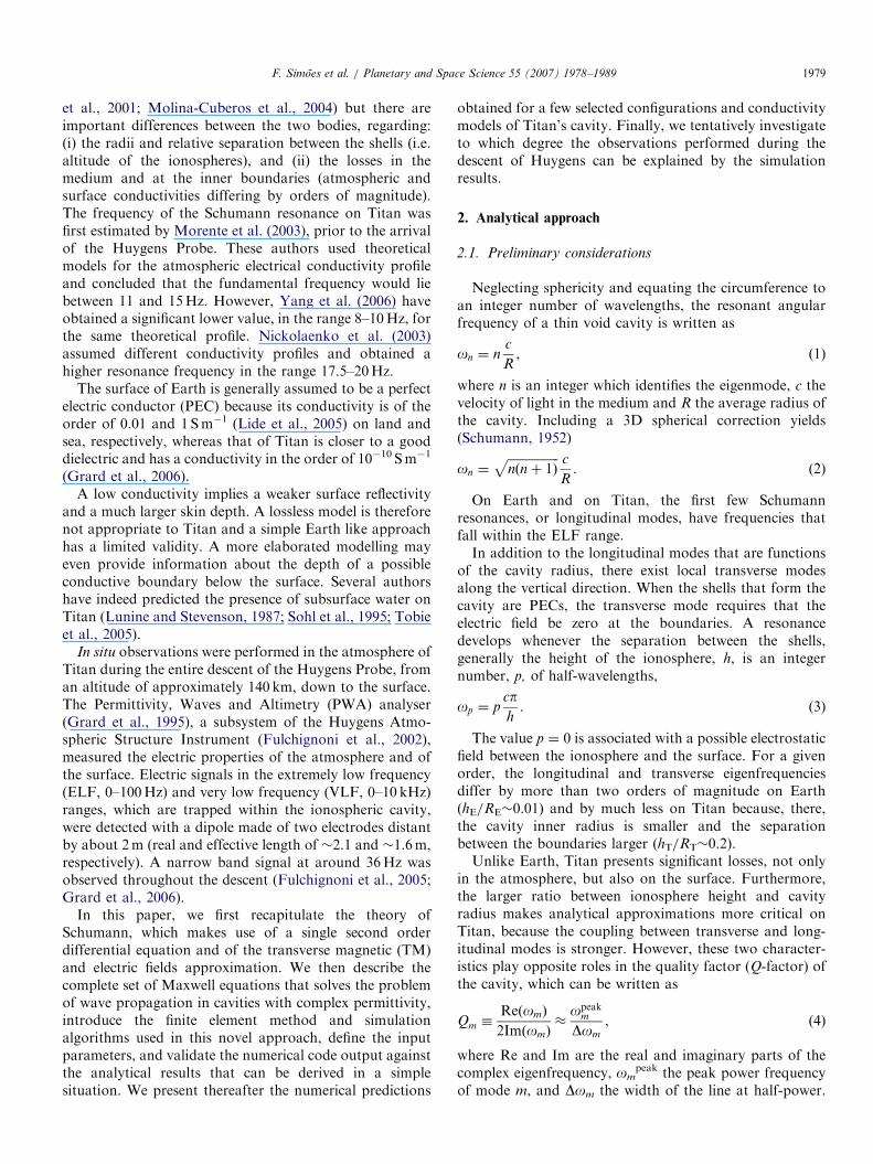
Planetary and Space Science 55 (2007) 1978–1989 A new numerical model for the simulation of ELF wave propagation and the computation of eigenmodes in the atmosphere of Titan: Did Huygens observe any Schumann resonance? F. Simo˜ es a, , R. Grard b , M. Hamelin a , J.J. Lo´pez-Moreno c , K. Schwingenschuh d , C. Be´ghin e , J.-J. Berthelier a , B. Besser d , V.J.G. Brown c , M. Chabassie`re e , P. Falkner b , F. Ferri f , M. Fulchignoni g , R. Hofe d , I. Jernej d , J.M. Jeronimo c , G.J. Molina-Cuberos h , R. Rodrigo c , H. Svedhem b , T. Tokano i , R. Trautner b a CETP/IPSL-CNRS 4, Avenue de Neptune, 94107 Saint Maur, France b RSSD, ESA-ESTEC, European Space Agency, Keplerlaan 1, 2200 AG Noordwijk, The Netherlands c Instituto de Astrofı´sica de Andalucı´a IAA-CSIC, Camino Bajo de Hue´tor 50, 18008 Granada, Spain d Space Research Institute, Austrian Academy of Sciences (IWF), Schmiedlstrasse 6, 8042 Graz, Austria e LPCE-CNRS 3A, Avenue de la Recherche Scientifique, 45071 Orle´ans cedex 2, France f CISAS ‘‘G. Colombo’’, Universita` di Padova, Via Venezia 15, 35131 Padova, Italy g LESIA, Observatoire de Paris, 5 Place Janssen, 92195 Meudon, France h Applied Electromagnetic Group, Department of Physics, University of Murcia, Murcia 30100, Spain i Institut fu ¨ r Geophysik und Meteorologie, Universita ¨t zu Ko¨ln, Albertus-Magnus-Platz, 50923 Ko¨ln, Germany Accepted 13 April 2007 Available online 27 April 2007 Abstract The propagation of extremely low frequency (ELF) electromagnetic waves in the Earth’s ionospheric cavity and the associated resonance phenomena have been extensively studied, in relation with lightning activity. We perform a similar investigation for Titan, the largest moon of Saturn. There are important differences between Earth and Titan, as far as the cavity geometry, the atmospheric electron density profile, and the surface conductivity are concerned. We present an improved 3D finite element model that provides an estimate of the lowest eigenfrequencies, associated quality factors (Q-factors), and ELF electric field spectra. The data collected by the electric antenna of the Permittivity, Waves, and Altimetry (PWA) instrument reveals the existence of a narrow-band signal at about 36 Hz during the entire descent of Huygens upon Titan. We assess the significance of these measurements against the model predictions, with due consideration to the experimental uncertainties. r 2007 Elsevier Ltd. All rights reserved. Keywords: Titan; Huygens probe; Atmospheric electricity; ELF electric field; Schumann resonance 1. Introduction The propagation of low frequency electromagnetic waves within the cavity formed by two, highly conductive, concentric, spherical shells, such as those formed by the surface and the ionosphere of Earth, was first studied by Schumann (1952) and was subsequently observed by Balser and Wagner (1960). When a cavity is excited with broadband electromagnetic sources, a resonant state can develop provided the average equatorial circumference is approximately equal to an integral number of wavelengths of the electromagnetic waves. This phenomenon is known as the Schumann resonance; it provides information about thunderstorm and lightning activity at Earth and acts, for example, as a ‘‘global tropical thermometer’’ (Williams, 1992). We shall apply the same approach to Saturn’s satellite. Titan and Earth are both wrapped up in thick atmo- spheres and conductive ionospheres (Schwingenschuh ARTICLE IN PRESS bwww.elsevier.com/locate/pss 0032-0633/$ - see front matter r 2007 Elsevier Ltd. All rights reserved. doi:10.1016/j.pss.2007.04.016 Corresponding author. Tel.: +33 1 4511 4273; fax: +33 1 48 89 44 33. E-mail address: [email protected] (F. Simo˜es).
Transcript of A new numerical model for the simulation of ELF wave propagation and the computation of eigenmodes...
ARTICLE IN PRESS
0032-0633/$ - se
doi:10.1016/j.ps
�CorrespondE-mail addr
Planetary and Space Science 55 (2007) 1978–1989
bwww.elsevier.com/locate/pss
A new numerical model for the simulation of ELF wave propagationand the computation of eigenmodes in the atmosphere of Titan:
Did Huygens observe any Schumann resonance?
F. Simoesa,�, R. Grardb, M. Hamelina, J.J. Lopez-Morenoc, K. Schwingenschuhd, C. Beghine,J.-J. Bertheliera, B. Besserd, V.J.G. Brownc, M. Chabassieree, P. Falknerb, F. Ferrif,
M. Fulchignonig, R. Hofed, I. Jernejd, J.M. Jeronimoc, G.J. Molina-Cuberosh, R. Rodrigoc,H. Svedhemb, T. Tokanoi, R. Trautnerb
aCETP/IPSL-CNRS 4, Avenue de Neptune, 94107 Saint Maur, FrancebRSSD, ESA-ESTEC, European Space Agency, Keplerlaan 1, 2200 AG Noordwijk, The NetherlandscInstituto de Astrofısica de Andalucıa IAA-CSIC, Camino Bajo de Huetor 50, 18008 Granada, Spain
dSpace Research Institute, Austrian Academy of Sciences (IWF), Schmiedlstrasse 6, 8042 Graz, AustriaeLPCE-CNRS 3A, Avenue de la Recherche Scientifique, 45071 Orleans cedex 2, France
fCISAS ‘‘G. Colombo’’, Universita di Padova, Via Venezia 15, 35131 Padova, ItalygLESIA, Observatoire de Paris, 5 Place Janssen, 92195 Meudon, France
hApplied Electromagnetic Group, Department of Physics, University of Murcia, Murcia 30100, SpainiInstitut fur Geophysik und Meteorologie, Universitat zu Koln, Albertus-Magnus-Platz, 50923 Koln, Germany
Accepted 13 April 2007
Available online 27 April 2007
Abstract
The propagation of extremely low frequency (ELF) electromagnetic waves in the Earth’s ionospheric cavity and the associated resonance
phenomena have been extensively studied, in relation with lightning activity. We perform a similar investigation for Titan, the largest moon of
Saturn. There are important differences between Earth and Titan, as far as the cavity geometry, the atmospheric electron density profile, and the
surface conductivity are concerned. We present an improved 3D finite element model that provides an estimate of the lowest eigenfrequencies,
associated quality factors (Q-factors), and ELF electric field spectra. The data collected by the electric antenna of the Permittivity, Waves, and
Altimetry (PWA) instrument reveals the existence of a narrow-band signal at about 36Hz during the entire descent of Huygens upon Titan. We
assess the significance of these measurements against the model predictions, with due consideration to the experimental uncertainties.
r 2007 Elsevier Ltd. All rights reserved.
Keywords: Titan; Huygens probe; Atmospheric electricity; ELF electric field; Schumann resonance
1. Introduction
The propagation of low frequency electromagneticwaves within the cavity formed by two, highly conductive,concentric, spherical shells, such as those formed by thesurface and the ionosphere of Earth, was first studied bySchumann (1952) and was subsequently observed by Balserand Wagner (1960). When a cavity is excited with
e front matter r 2007 Elsevier Ltd. All rights reserved.
s.2007.04.016
ing author. Tel.: +331 4511 4273; fax: +33 1 48 89 44 33.
ess: [email protected] (F. Simoes).
broadband electromagnetic sources, a resonant state candevelop provided the average equatorial circumference isapproximately equal to an integral number of wavelengthsof the electromagnetic waves. This phenomenon is knownas the Schumann resonance; it provides information aboutthunderstorm and lightning activity at Earth and acts, forexample, as a ‘‘global tropical thermometer’’ (Williams,1992). We shall apply the same approach to Saturn’ssatellite.Titan and Earth are both wrapped up in thick atmo-
spheres and conductive ionospheres (Schwingenschuh
ARTICLE IN PRESSF. Simoes et al. / Planetary and Space Science 55 (2007) 1978–1989 1979
et al., 2001; Molina-Cuberos et al., 2004) but there areimportant differences between the two bodies, regarding:(i) the radii and relative separation between the shells (i.e.altitude of the ionospheres), and (ii) the losses in themedium and at the inner boundaries (atmospheric andsurface conductivities differing by orders of magnitude).The frequency of the Schumann resonance on Titan wasfirst estimated by Morente et al. (2003), prior to the arrivalof the Huygens Probe. These authors used theoreticalmodels for the atmospheric electrical conductivity profileand concluded that the fundamental frequency would liebetween 11 and 15Hz. However, Yang et al. (2006) haveobtained a significant lower value, in the range 8–10Hz, forthe same theoretical profile. Nickolaenko et al. (2003)assumed different conductivity profiles and obtained ahigher resonance frequency in the range 17.5–20Hz.
The surface of Earth is generally assumed to be a perfectelectric conductor (PEC) because its conductivity is of theorder of 0.01 and 1 Sm�1 (Lide et al., 2005) on land andsea, respectively, whereas that of Titan is closer to a gooddielectric and has a conductivity in the order of 10�10 Sm�1
(Grard et al., 2006).A low conductivity implies a weaker surface reflectivity
and a much larger skin depth. A lossless model is thereforenot appropriate to Titan and a simple Earth like approachhas a limited validity. A more elaborated modelling mayeven provide information about the depth of a possibleconductive boundary below the surface. Several authorshave indeed predicted the presence of subsurface water onTitan (Lunine and Stevenson, 1987; Sohl et al., 1995; Tobieet al., 2005).
In situ observations were performed in the atmosphere ofTitan during the entire descent of the Huygens Probe, froman altitude of approximately 140 km, down to the surface.The Permittivity, Waves and Altimetry (PWA) analyser(Grard et al., 1995), a subsystem of the Huygens Atmo-spheric Structure Instrument (Fulchignoni et al., 2002),measured the electric properties of the atmosphere and ofthe surface. Electric signals in the extremely low frequency(ELF, 0–100Hz) and very low frequency (VLF, 0–10 kHz)ranges, which are trapped within the ionospheric cavity,were detected with a dipole made of two electrodes distantby about 2m (real and effective length of �2.1 and �1.6m,respectively). A narrow band signal at around 36Hz wasobserved throughout the descent (Fulchignoni et al., 2005;Grard et al., 2006).
In this paper, we first recapitulate the theory ofSchumann, which makes use of a single second orderdifferential equation and of the transverse magnetic (TM)and electric fields approximation. We then describe thecomplete set of Maxwell equations that solves the problemof wave propagation in cavities with complex permittivity,introduce the finite element method and simulationalgorithms used in this novel approach, define the inputparameters, and validate the numerical code output againstthe analytical results that can be derived in a simplesituation. We present thereafter the numerical predictions
obtained for a few selected configurations and conductivitymodels of Titan’s cavity. Finally, we tentatively investigateto which degree the observations performed during thedescent of Huygens can be explained by the simulationresults.
2. Analytical approach
2.1. Preliminary considerations
Neglecting sphericity and equating the circumference toan integer number of wavelengths, the resonant angularfrequency of a thin void cavity is written as
on ¼ nc
R, (1)
where n is an integer which identifies the eigenmode, c thevelocity of light in the medium and R the average radius ofthe cavity. Including a 3D spherical correction yields(Schumann, 1952)
on ¼ffiffiffiffiffiffiffiffiffiffiffiffiffiffiffiffiffinðnþ 1Þ
p c
R. (2)
On Earth and on Titan, the first few Schumannresonances, or longitudinal modes, have frequencies thatfall within the ELF range.In addition to the longitudinal modes that are functions
of the cavity radius, there exist local transverse modesalong the vertical direction. When the shells that form thecavity are PECs, the transverse mode requires that theelectric field be zero at the boundaries. A resonancedevelops whenever the separation between the shells,generally the height of the ionosphere, h, is an integernumber, p, of half-wavelengths,
op ¼ pcph. (3)
The value p ¼ 0 is associated with a possible electrostaticfield between the ionosphere and the surface. For a givenorder, the longitudinal and transverse eigenfrequenciesdiffer by more than two orders of magnitude on Earth(hE/RE�0.01) and by much less on Titan because, there,the cavity inner radius is smaller and the separationbetween the boundaries larger (hT/RT�0.2).Unlike Earth, Titan presents significant losses, not only
in the atmosphere, but also on the surface. Furthermore,the larger ratio between ionosphere height and cavityradius makes analytical approximations more critical onTitan, because the coupling between transverse and long-itudinal modes is stronger. However, these two character-istics play opposite roles in the quality factor (Q-factor) ofthe cavity, which can be written as
Qm �ReðomÞ
2ImðomÞ�
opeakm
Dom
, (4)
where Re and Im are the real and imaginary parts of thecomplex eigenfrequency, om
peak the peak power frequencyof mode m, and Dom the width of the line at half-power.
ARTICLE IN PRESSF. Simoes et al. / Planetary and Space Science 55 (2007) 1978–19891980
Although the cavity of Titan is more intricate than that ofEarth, an expedient way of estimating the Q-factor con-sists in using the ratio between the resonator thickness andthe skin depth of the electric field (Nickolaenko andHayakawa, 2002). The latter is given by Balanis (1989) as
dh ¼
ffiffiffiffiffiffiffiffiffi2
mo�o
s ffiffiffiffiffiffiffiffiffiffiffiffiffiffiffiffiffiffiffiffiffiffiffiffiffiffi1þ ðs=o�oÞ
2q
� 1
� ��1=2o
, (5)
where eo and mo are the permittivity and magneticpermeability of vacuum, o the angular frequency of thepropagating wave, and s the medium conductivity.
Thus Qph/dh, in first approximation. Increasing theionosphere height augments the Q-factor, whereas lossesare more important when the boundary is poorly conduct-ing and the skin depth large.
Geometric optics is not a good approximation for thecalculation of cavity losses and is not strictly applicable inthe ELF–VLF range, but the ray tracing technique stillprovides qualitative information about the variation of theQ-factor with boundary separation. The minimum numberof reflections required for circling a void cavity of inner andouter radii, Rint and Rext,
nR ¼p
cos�1ðRint=RextÞ, (6)
is approximately 5 for Titan and 22 for Earth. Other thingsbeing equal, a lower number of reflections are required in athicker cavity, which confirms that increasing the distancebetween the boundaries reduces the losses in the system.A more accurate model should include the losses due to theatmosphere, in addition to those due to the boundaries,which also lowers the theoretical value of the Schumannresonance on Titan (Morente et al., 2003; Molina-Cuberoset al., 2004).
2.2. Formulation of the resonant cavity
A full treatment of the Schumann resonance in the cavityof Titan requires the solution of Maxwell equations,
r � E ¼ �qB
qt, (7)
r �H ¼ sE þqD
qt, (8)
D ¼ ��oE; B ¼ moH , (9)
where E and D are the electric and displacement fields, Hand B the magnetic field strength and flux density, and e therelative permittivity.
Taking into account the cavity characteristics anddecoupling the electric and magnetic fields, Eqs. (7)–(9)can be solved in spherical coordinates, using the harmonicpropagation approximation. One mode is characterized byHr ¼ 0 and is called the TM wave, the other one by Er ¼ 0and is known as the transverse electric (TE) wave.
Neglecting the day–night asymmetry of the ionosphere,the standard method of separation of variables yields(Bliokh et al., 1980)
d2
dr2�
nðnþ 1Þ
r2þ
o2
c2�ðrÞ �
ffiffiffiffiffiffiffi�ðrÞ
p d2
dr21ffiffiffiffiffiffiffi�ðrÞ
p !( )
rRðrÞð Þ ¼ 0,
(10)
where R(r) is a radial function related to the electric andmagnetic fields by the Debye potentials (Wait, 1962). Thisequation gives the eigenvalues of the longitudinal andtransverse modes, assuming either dR(r)/dr ¼ 0 or R(r) ¼ 0at both boundaries, respectively. For a thin void cavity theeigenvalues are those given by Eqs. (2) and (3). However,the previous approximation is no longer valid and Eq. (10)is not sufficiently accurate for thick cavities, such as that ofTitan, because the coupling between longitudinal andtransverse modes is strong. A numerical computation,based on a finite element model and including not onlylosses in the atmosphere but also on the surface, istherefore required.
3. The numerical approach
3.1. Model inputs
The numerical algorithms that solve the resonant cavityproblem from Eqs. (7)–(9) are implemented with the finiteelement method (Zimmerman, 2006). The meshes arecomposed of 5� 104 and 106 elements in the 2D and 3Dapproximations, respectively. Comparing the results ob-tained in 2D and 3D, when axial symmetry applies, assessesthe accuracy. Continuity conditions are imposed at thesurface of Titan unless the latter coincides with the innerboundary of the cavity (Fig. 1).The numerical algorithms require the following model
inputs:
(a)
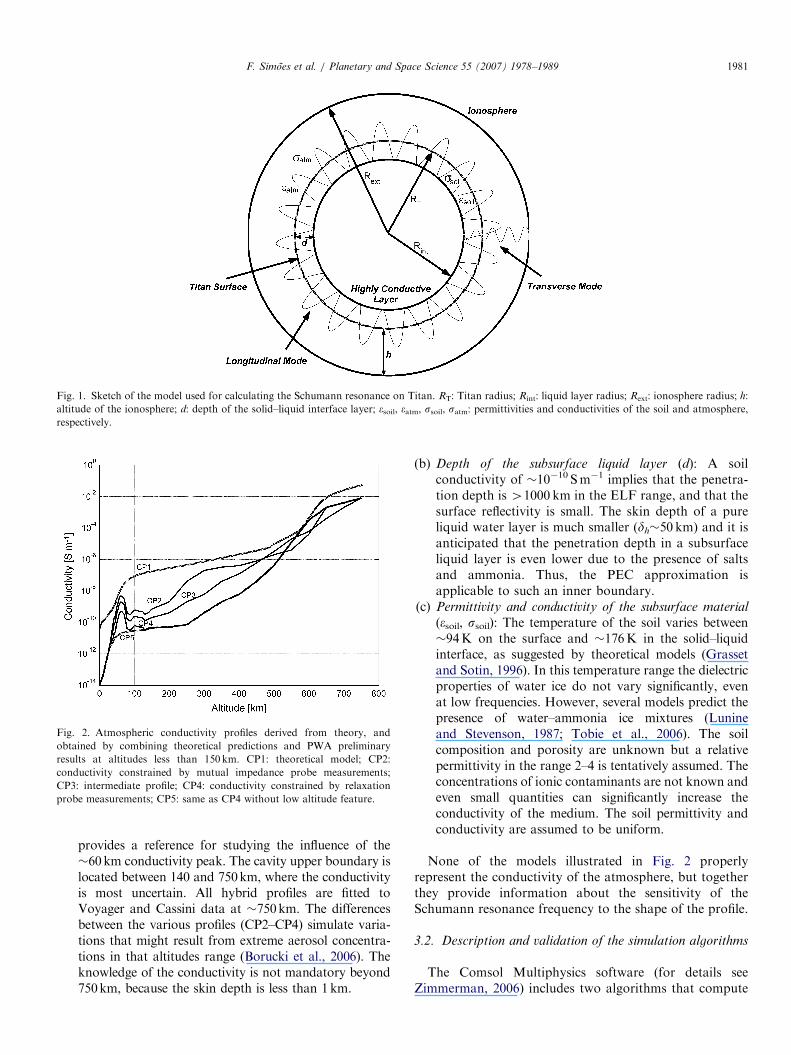
Conductivity of the atmosphere and lower ionosphere(satm): Several atmospheric conductivity profiles areshown in Fig. 2. The conductivity CP1 is derived fromtheoretical predictions (Borucki et al., 1987; Molina-Cuberos et al., 2004). This profile can be adjusted inmany ways to yield a number of hybrid profiles,CP2–CP5, which combine both theoretical and experi-mental inputs. Although the analysis of the PWA data isnot finalized yet, preliminary conductivity profiles ataltitudes less than 140km have been obtained with themutual impedance (Hamelin et al., 2007) and relaxationprobes. The hybrid conductivity profiles are constrainedby the measurements obtained with these two sensors.A peak in conductivity, at around 60km, has beenobserved with PWA during the descent (Grard et al.,2006), which introduces a new feature in the profile; italso appears that the theoretical models tend to over-estimate the electron conductivity by as much as twoorders of magnitude at �100km. The CP5 profile
ARTICLE IN PRESS
Fig. 2. Atmospheric conductivity profiles derived from theory, and
obtained by combining theoretical predictions and PWA preliminary
results at altitudes less than 150 km. CP1: theoretical model; CP2:
conductivity constrained by mutual impedance probe measurements;
CP3: intermediate profile; CP4: conductivity constrained by relaxation
probe measurements; CP5: same as CP4 without low altitude feature.
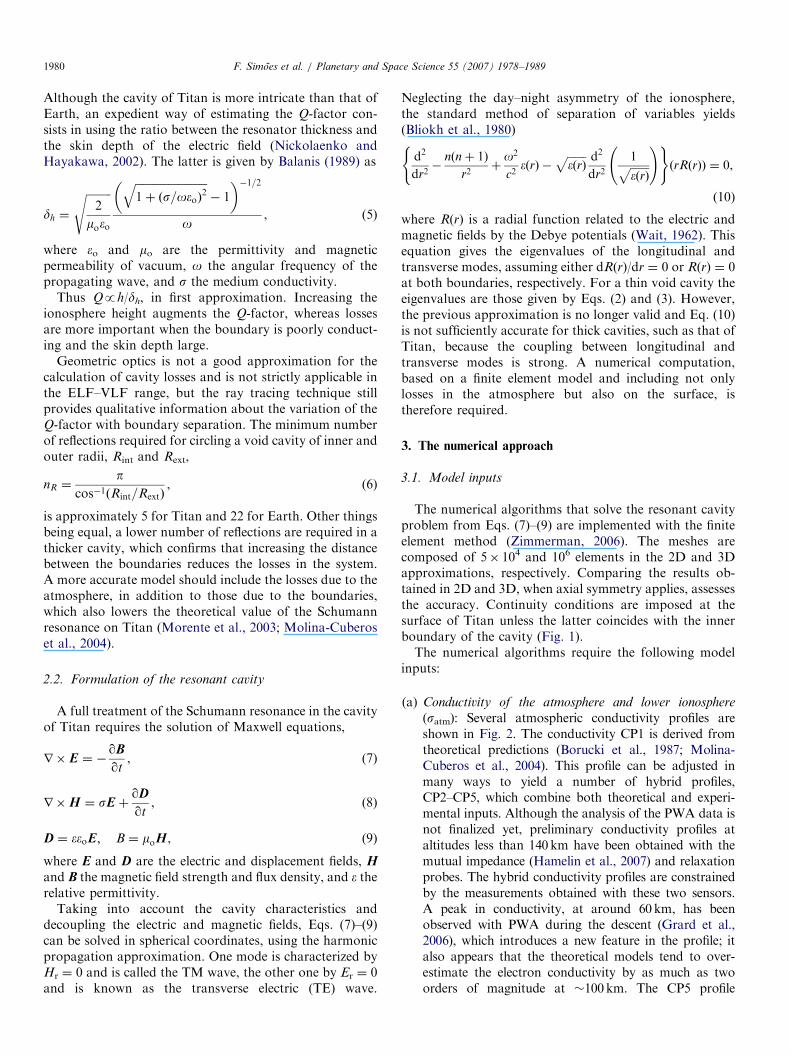
Fig. 1. Sketch of the model used for calculating the Schumann resonance on Titan. RT: Titan radius; Rint: liquid layer radius; Rext: ionosphere radius; h:
altitude of the ionosphere; d: depth of the solid–liquid interface layer; esoil, eatm, ssoil, satm: permittivities and conductivities of the soil and atmosphere,
respectively.
F. Simoes et al. / Planetary and Space Science 55 (2007) 1978–1989 1981
provides a reference for studying the influence of the�60km conductivity peak. The cavity upper boundary islocated between 140 and 750km, where the conductivityis most uncertain. All hybrid profiles are fitted toVoyager and Cassini data at �750km. The differencesbetween the various profiles (CP2–CP4) simulate varia-tions that might result from extreme aerosol concentra-tions in that altitudes range (Borucki et al., 2006). Theknowledge of the conductivity is not mandatory beyond750km, because the skin depth is less than 1km.
(b)
Depth of the subsurface liquid layer (d): A soilconductivity of �10�10 Sm�1 implies that the penetra-tion depth is 41000 km in the ELF range, and that thesurface reflectivity is small. The skin depth of a pureliquid water layer is much smaller (dh�50 km) and it isanticipated that the penetration depth in a subsurfaceliquid layer is even lower due to the presence of saltsand ammonia. Thus, the PEC approximation isapplicable to such an inner boundary.(c)
Permittivity and conductivity of the subsurface material(esoil, ssoil): The temperature of the soil varies between�94K on the surface and �176K in the solid–liquidinterface, as suggested by theoretical models (Grassetand Sotin, 1996). In this temperature range the dielectricproperties of water ice do not vary significantly, evenat low frequencies. However, several models predict thepresence of water–ammonia ice mixtures (Lunineand Stevenson, 1987; Tobie et al., 2006). The soilcomposition and porosity are unknown but a relativepermittivity in the range 2–4 is tentatively assumed. Theconcentrations of ionic contaminants are not known andeven small quantities can significantly increase theconductivity of the medium. The soil permittivity andconductivity are assumed to be uniform.
None of the models illustrated in Fig. 2 properlyrepresent the conductivity of the atmosphere, but togetherthey provide information about the sensitivity of theSchumann resonance frequency to the shape of the profile.
3.2. Description and validation of the simulation algorithms
The Comsol Multiphysics software (for details seeZimmerman, 2006) includes two algorithms that compute
ARTICLE IN PRESS
Table 1
Comparison between the eigenfrequencies derived from the analytical and
numerical models. Inner shell radii RT ¼ 2575 km and RE ¼ 6370 km
Cavity Test Spherical approximation
(Eq. (10))
Finite element model
Longitudinal
(Hz)
Transverse
(Hz)
Longitudinal
(Hz)
Transverse
(Hz)
Earth A 10.6 – 10.6 –
B 10.5 1998 10.6 2008
C 10.3 1670 8.86 1635
Titan A 26.2 – 26.2 –
B 22.9 201.2 23.1 201.2
C 14.3 168.1 19.1 163.5
(A): h-0, satm ¼ 0, and eatm ¼ 1; (B): Height of ionospheric boundaries
hT ¼ 750km and hE ¼ 75 km, satm ¼ 0, and eatm ¼ 1; (C): Same as in (B),
but the permittivity profile is represented by a sigmoid-type function, in
the range 1–2. Perfect electric conductor boundaries are considered in all
cases. The dimensions of Titan and Earth are identified by the subscripts T
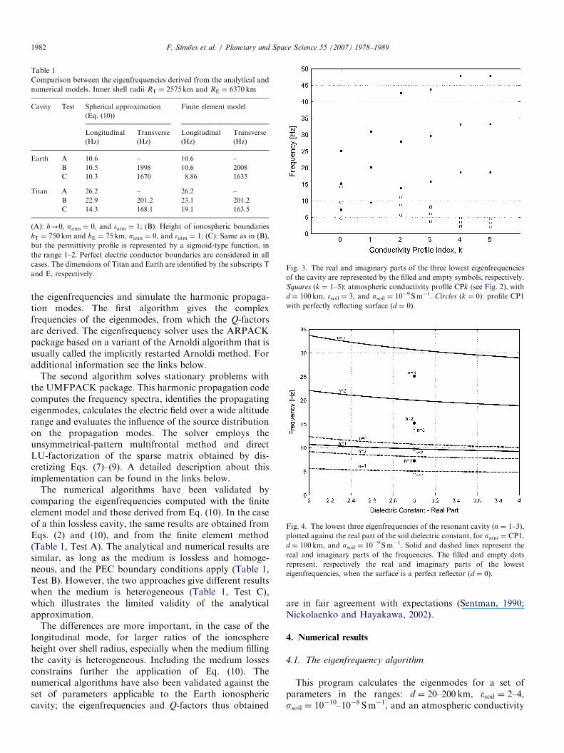
and E, respectively.Fig. 3. The real and imaginary parts of the three lowest eigenfrequencies
of the cavity are represented by the filled and empty symbols, respectively.
Squares (k ¼ 1–5): atmospheric conductivity profile CPk (see Fig. 2), with
d ¼ 100 km, esoil ¼ 3, and ssoil ¼ 10�9 Sm�1. Circles (k ¼ 0): profile CP1
with perfectly reflecting surface (d ¼ 0).
Fig. 4. The lowest three eigenfrequencies of the resonant cavity (n ¼ 1–3),
plotted against the real part of the soil dielectric constant, for satm ¼ CP1,
d ¼ 100 km, and ssoil ¼ 10�9 Sm�1. Solid and dashed lines represent the
real and imaginary parts of the frequencies. The filled and empty dots
represent, respectively the real and imaginary parts of the lowest
eigenfrequencies, when the surface is a perfect reflector (d ¼ 0).
F. Simoes et al. / Planetary and Space Science 55 (2007) 1978–19891982
the eigenfrequencies and simulate the harmonic propaga-tion modes. The first algorithm gives the complexfrequencies of the eigenmodes, from which the Q-factorsare derived. The eigenfrequency solver uses the ARPACKpackage based on a variant of the Arnoldi algorithm that isusually called the implicitly restarted Arnoldi method. Foradditional information see the links below.
The second algorithm solves stationary problems withthe UMFPACK package. This harmonic propagation codecomputes the frequency spectra, identifies the propagatingeigenmodes, calculates the electric field over a wide altituderange and evaluates the influence of the source distributionon the propagation modes. The solver employs theunsymmetrical-pattern multifrontal method and directLU-factorization of the sparse matrix obtained by dis-cretizing Eqs. (7)–(9). A detailed description about thisimplementation can be found in the links below.
The numerical algorithms have been validated bycomparing the eigenfrequencies computed with the finiteelement model and those derived from Eq. (10). In the caseof a thin lossless cavity, the same results are obtained fromEqs. (2) and (10), and from the finite element method(Table 1, Test A). The analytical and numerical results aresimilar, as long as the medium is lossless and homoge-neous, and the PEC boundary conditions apply (Table 1,Test B). However, the two approaches give different resultswhen the medium is heterogeneous (Table 1, Test C),which illustrates the limited validity of the analyticalapproximation.
The differences are more important, in the case of thelongitudinal mode, for larger ratios of the ionosphereheight over shell radius, especially when the medium fillingthe cavity is heterogeneous. Including the medium lossesconstrains further the application of Eq. (10). Thenumerical algorithms have also been validated against theset of parameters applicable to the Earth ionosphericcavity; the eigenfrequencies and Q-factors thus obtained
are in fair agreement with expectations (Sentman, 1990;Nickolaenko and Hayakawa, 2002).
4. Numerical results
4.1. The eigenfrequency algorithm
This program calculates the eigenmodes for a set ofparameters in the ranges: d ¼ 20–200 km, esoil ¼ 2–4,ssoil ¼ 10�10–10�8 Sm�1, and an atmospheric conductivity
ARTICLE IN PRESSF. Simoes et al. / Planetary and Space Science 55 (2007) 1978–1989 1983
profile satm represented by one of the CP1–CP5 modelsdisplayed in Fig. 2. Figs. 3–6 show the variations of the realand imaginary parts of the three lowest eigenfrequencies asfunctions of those parameters. The atmospheric conduc-tivity, the presence of aerosols and the depth of theconductive boundary have a profound influence upon the
Table 2
Comparison between the lowest eigenfrequency modes (Hz) on Titan for diffe
boundaries are located at Rint ¼ RT and Rext ¼ RT+hT
Profile mode CP1 CP2 CP3
First 7.27+4.77i 13.43+6.25i 16.0
Second 15.25+9.71i 28.13+10.57i 30.2
Third 25.31+14.80i 43.93+13.64i 44.9
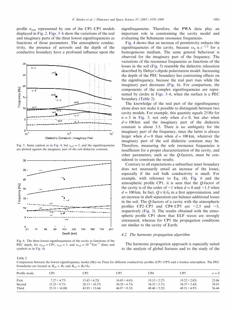
Fig. 5. Same caption as in Fig. 4, but esoil ¼ 3, and the eigenfrequencies
are plotted against the imaginary part of the soil dielectric constant.
Fig. 6. The three lowest eigenfrequencies of the cavity as functions of the
PEC depth, for satm ¼ CP1, esoil ¼ 3, and ssoil ¼ 10�9 Sm�1 (lines and
symbols as in Fig. 4).
eigenfrequencies. Therefore, the PWA data play animportant role in constraining the cavity model andevaluating the Schumann resonance frequencies.Fig. 4 shows that an increase of permittivity reduces the
eigenfrequencies of the cavity, because on / ��1=2 for ahomogeneous medium. The same general behaviour isobserved for the imaginary part of the frequency. Thevariations of the resonance frequencies as functions of thelosses in the soil (Fig. 5) resemble the dielectric relaxationdescribed by Debye’s dipole polarization model. Increasingthe depth of the PEC boundary has contrasting effects onthe eigenfrequency, because the real part rises while theimaginary part decreases (Fig. 6). For comparison, thecomponents of the complex eigenfrequencies are repre-sented by circles in Figs. 3–6, when the surface is a PECboundary (Table 2).The knowledge of the real part of the eigenfrequency
alone does not make it possible to distinguish between twocavity models. For example, this quantity equals 25Hz forn ¼ 3 in Fig. 5, not only when d ¼ 0, but also whend ¼ 100 km and the imaginary part of the dielectricconstant is about 3.5. There is no ambiguity for theimaginary part of the frequency, since the latter is alwayslarger when d ¼ 0 than when d ¼ 100 km, whatever theimaginary part of the soil dielectric constant may be.Therefore, measuring the sole resonance frequencies isinsufficient for a proper characterization of the cavity, andother parameters, such as the Q-factors, must be con-sidered to constrain the results.Contrary to all expectations a subsurface inner boundary
does not necessarily entail an increase of the losses,especially if the soil bulk conductivity is small. Forexample, with reference to Eq. (4), Fig. 6 and theatmospheric profile CP1, it is seen that the Q-factor ofthe cavity is of the order of �1 when d ¼ 0 and �1.5 whend ¼ 100 km. In fact, Qph/dh in a first approximation, andan increase in shell separation can balance additional lossesin the soil. The Q-factors of a cavity with the atmosphericprofiles CP2–CP3 and CP4–CP5 are �2.5 and �5,respectively (Fig. 3). The results obtained with the atmo-spheric profile CP1 show that ELF waves are stronglyattenuated, whereas for CP5 the propagation conditionsare similar to the cavity of Earth.
4.2. The harmonic propagation algorithm
The harmonic propagation approach is especially suitedto the analysis of global features and to the study of the
rent conductivity profiles (CP1–CP5) and a lossless atmosphere. The PEC
CP4 CP5 s ¼ 0
5+4.01i 19.15+2.27i 19.22+2.02i 23.06
9+6.73i 34.32+3.71i 34.37+3.45i 39.93
7+9.32i 49.48+5.22i 49.51+4.97i 56.44
ARTICLE IN PRESS
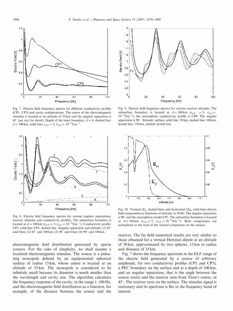
Fig. 7. Electric field frequency spectra for different conductivity profiles
(CP1, CP3) and cavity configurations. The centre of the electromagnetic
stimulus is located at an altitude of 35 km and the angular separation is
451 (see text for detail). Depth of the inner boundary: d ¼ 0, dashed line;
d ¼ 100km, solid line; esoil ¼ 3; ssoil ¼ 10�9 Sm�1.
Fig. 8. Electric field frequency spectra for various angular separations,
receiver altitudes and conductivity profiles. The subsurface boundary is
located at d ¼ 100 km (esoil ¼ 3; ssoil ¼ 10�9 Sm�1). Conductivity profile:
CP3, solid line; CP1, dashed line. Angular separation and altitude: (1) 451
and 0 km; (2) 451 and 100km; (3) 901 and 0 km; (4) 901 and 100 km.
Fig. 9. Electric field frequency spectra for various receiver altitudes. The
subsurface boundary is located at d ¼ 100km (esoil ¼ 3; ssoil ¼10�9 Sm�1); the atmospheric conductivity profile is CP4. The angular
separation is 901. Altitude: surface, solid line; 50 km, dashed line; 100 km,
dotted line; 150 km, dashed–dotted line.
Fig. 10. Vertical (EV, dashed line) and horizontal (EH, solid line) electric
field components as functions of altitude, at 36Hz. The angular separation
is 901 and the atmospheric model CP2. The subsurface boundary is located
at d ¼ 100 km (esoil ¼ 3; ssoil ¼ 10�9 Sm�1). Both components are
normalized to the level of the vertical component on the surface.
F. Simoes et al. / Planetary and Space Science 55 (2007) 1978–19891984
electromagnetic field distribution generated by sparsesources. For the sake of simplicity, we shall assume alocalized electromagnetic stimulus. The source is a pulsa-ting monopole defined by an equipotential sphericalsurface of radius 15 km, whose centre is located at analtitude of 35 km. The monopole is considered to beinfinitely small because its diameter is much smaller thanthe wavelength and cavity size. The algorithm calculatesthe frequency response of the cavity, in the range 1–100Hz,and the electromagnetic field distribution as a function, forexample, of the distance between the source and the
receiver. The far field numerical results are very similar tothose obtained for a vertical Hertzian dipole at an altitudeof 50 km, approximated by two spheres, 15 km in radiusand distance of 35 km.Fig. 7 shows the frequency spectrum in the ELF range of
the electric field generated by a source of arbitraryamplitude, for two conductivity profiles (CP1 and CP3),a PEC boundary on the surface and at a depth of 100 km,and an angular separation, that is the angle between thesource centre and the receiver seen from Titan’s centre, of451. The receiver rests on the surface. The stimulus signal isstationary and its spectrum is flat in the frequency band ofinterest.
ARTICLE IN PRESS
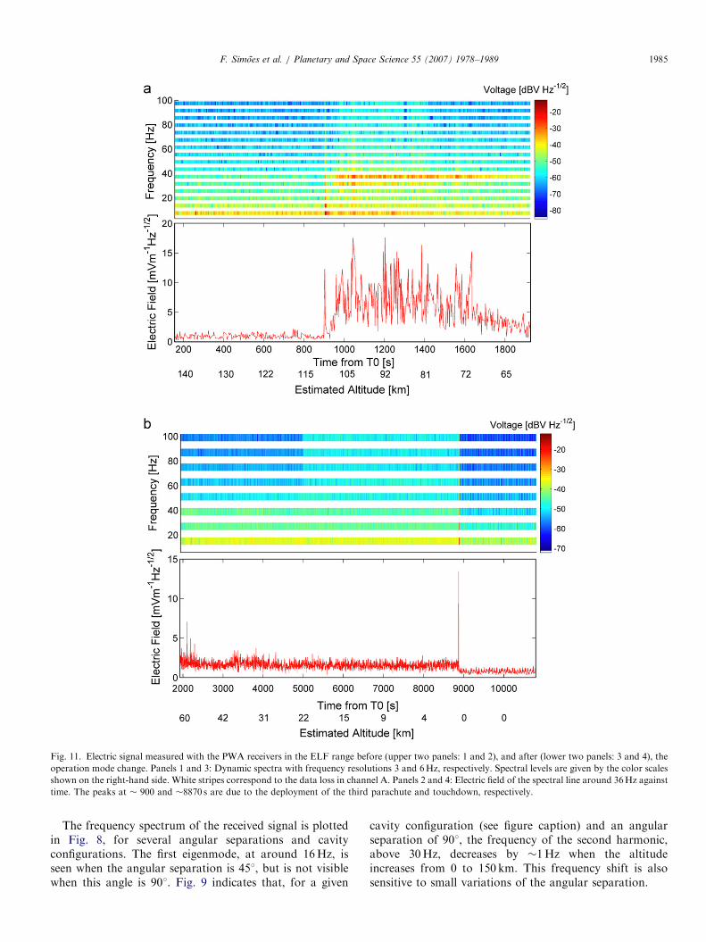
Fig. 11. Electric signal measured with the PWA receivers in the ELF range before (upper two panels: 1 and 2), and after (lower two panels: 3 and 4), the
operation mode change. Panels 1 and 3: Dynamic spectra with frequency resolutions 3 and 6Hz, respectively. Spectral levels are given by the color scales
shown on the right-hand side. White stripes correspond to the data loss in channel A. Panels 2 and 4: Electric field of the spectral line around 36Hz against
time. The peaks at � 900 and �8870 s are due to the deployment of the third parachute and touchdown, respectively.
F. Simoes et al. / Planetary and Space Science 55 (2007) 1978–1989 1985
The frequency spectrum of the received signal is plottedin Fig. 8, for several angular separations and cavityconfigurations. The first eigenmode, at around 16Hz, isseen when the angular separation is 451, but is not visiblewhen this angle is 901. Fig. 9 indicates that, for a given
cavity configuration (see figure caption) and an angularseparation of 901, the frequency of the second harmonic,above 30Hz, decreases by �1Hz when the altitudeincreases from 0 to 150 km. This frequency shift is alsosensitive to small variations of the angular separation.
ARTICLE IN PRESS
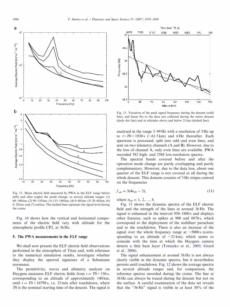
Fig. 12. Mean electric field measured by PWA in the ELF range before
(left) and after (right) the mode change, in several altitude ranges: (1)
60–140 km; (2) 80–110 km; (3) 115–140km; (4) 0–60 km; (5) 20–60 km; (6)
0–20 km; and (7) surface. The dashed lines represent the signal level during
the cruise.
Fig. 13. Variation of the peak signal frequency during the descent (solid
line), and linear fits to the data sets collected during the entire descent
(dash–dot line) and at altitudes above and below 21 km (dashed line).
F. Simoes et al. / Planetary and Space Science 55 (2007) 1978–19891986
Fig. 10 shows how the vertical and horizontal compo-nents of the electric field vary with altitude for theatmospheric profile CP2, at 36Hz.
5. The PWA measurements in the ELF range
We shall now present the ELF electric field observationsperformed in the atmosphere of Titan and, with referenceto the numerical simulation results, investigate whetherthey display the spectral signature of a Schumannresonance.
The permittivity, waves and altimetry analyser onHuygens measures ELF electric fields from t ¼ T0+156 s,corresponding to an altitude of approximately 140 km,until t ¼ T0+10798 s, i.e. 32min after touchdown, whereT0 is the nominal starting time of the descent. The signal is
analysed in the range 3–99Hz with a resolution of 3Hz upto t�T0+1930 s (�61.5 km) and 6Hz thereafter. Eachspectrum is processed, split into odd and even lines, andsent on two telemetry channels (A and B). However, due tothe loss of channel A, only even lines are available. PWArecorded 582 high- and 2588 low-resolution spectra.The spectral bands covered before and after the
operation mode change are partly overlapping and partlycomplementary. However, due to the data loss, about onequarter of the ELF range is not covered at all during thewhole descent. This domain consists of 3Hz stripes centredon the frequencies
f ab ¼ 3ð4nab � 3Þ, (11)
where nab ¼ 1, 2,y, 8.Fig. 11 shows the dynamic spectra of the ELF electric
field and the strength of the lines at around 36Hz. Thesignal is enhanced in the interval 950–1800 s and displaysother features, such as spikes at 900 and 8870 s, whichcorrespond to the deployment of the stabilizer parachuteand to the touchdown. There is also an increase of thesignal over the whole frequency range at �5000 s (corre-sponding to an altitude of �21 km), which seems tocoincide with the time at which the Huygens cameradetects a thin haze layer (Tomasko et al., 2005; Grardet al., 2006).The signal enhancement at around 36Hz is not always
clearly visible in the dynamic spectra, but it neverthelesspersists until touchdown. Fig. 12 shows the average spectrain several altitude ranges and, for comparison, thereference spectra recorded during the cruise. The line at36Hz can always be traced during the descent but not onthe surface. A careful examination of the data set revealsthat the ‘‘36Hz’’ signal is visible in at least 50% of the
ARTICLE IN PRESSF. Simoes et al. / Planetary and Space Science 55 (2007) 1978–1989 1987
spectra in the terminal phase of the descent and during upto 95% of the times when its amplitude is enhanced.
The data sets recorded before and after the operationmode change are split in bins of 50 and 100 spectra,respectively, and the weighted arithmetic mean frequencyof the emission, i.e. the average value of the 36Hz andadjacent lines, is evaluated within each bin. The output ofthis crude analysis is reported in Fig. 13 and indicates thatthe peak frequency increases by about 1.5Hz throughoutthe descent. The frequency is also sensitive to smallvariations of the angular separation.
6. Discussion and conclusion
Titan offers peculiarities different from those of Earth.The geometry of Titan’s cavity is such that the eigenfre-quencies of the longitudinal and transverse modes arecoupled, which precludes the use of analytical approxima-tions. The low conductivity (�10�10 Sm�1) and lowreflectivity of the soil also call for a more elaboratedapproach, but make it possible to study the subsurface andto search for the ocean predicted by theoretical models,provided the electric properties of the soil vary little withdepth (Figs. 1 and 3). The conductivity peak at 60 km splitsthe cavity in two sectors, influences the propagation ofwaves and enhances the electric field strength in the upperatmosphere (Fig. 10).
The novelty of this numerical approach is threefold:
(1)
Maxwell equations are solved with the finite elementmethod, whereas most previous efforts were based onsemi-analytical approximations or TLM (transmissionline model) and FDTD (finite difference time domain)numerical models.(2)
The conductivity profiles of the cavity are morerealistic, since they are partly constrained by themeasurements of the PWA–Huygens instrument, atlow altitudes, and the Voyager and Cassini results, athigh altitudes.(3)
The wave propagation simulation takes into accountthe effect of subsurface losses.The simulation results provides an overview of the ELFwave distribution in the resonant cavity; the eigenfrequen-cies and Q-factors obtained with CP1 lie in the same rangeas those presented by Yang et al. (2006) with the FDTDapproach. A significant aerosol concentration at highaltitude increases the Q-factor (Eq. (4), Table 2), whichcan be higher than on Earth.
The ELF electric field measurements performed duringthe descent of the Huygens Probe through the atmosphereof Titan reveals the existence of a narrow-band emission ataround 36Hz (Fig. 11). The maximum and averageamplitudes recorded during the descent are 17.5 and2mVm�1Hz�1/2, respectively; the mean frequency in-creases steadily during the descent, from 35Hz at 140 kmto 37Hz before touchdown (Fig. 13). The transition at an
altitude of about 21 km (Fig. 11) seems to match theoccurrence of a thin haze layer imaged by the cameraonboard the Probe. If one discards the frequency pointsmeasured at altitudes less than �21 km, then the meanvariation observed in Fig. 13 is close to 1Hz.For most cavity models, a spectral peak at 36Hz can
match the second eigenfrequency (Fig. 3). Furthermore, thelowest eigenmode is either matching an absent line or thecorresponding amplitude is small. The latter phenomenoncan be understood if the angular separation between thesource and the receiver is close to 901; the amplitude of thefirst eigenmode is negligible and only the second one ismeasurable (Fig. 8). Another possible, though less likely,reason for the absence of the fundamental mode is that itsfrequency coincides with the second missing spectral line(nab ¼ 2 in Eq. (11)).The peak spectral frequencies associated with a source at
high latitude (angular separation �901) vary with thealtitude of the receiver (Fig. 9). The frequency of thesecond eigenmode (�32Hz) increases, for example, byapproximately 1Hz between an altitude of 150 km and thesurface, in good agreement with the experimental resultsreported in Fig. 13; the variation can be larger if a smalldeviation of the angular separation is also taken intoaccount (see the Huygens Probe descent trajectory;Lebreton et al., 2005).The model polarization profile of the electric field is
illustrated in Fig. 10. The horizontal component is roughlyone order of magnitude smaller than the vertical one; itshows a trough that matches the conductivity peak, inaccordance with Ampere law, and a peak close to 170 km.The PWA dipole is approximately horizontal and thevariation of the ‘‘36Hz’’ level with altitude (see Figs. 11and 12) should be compared, in first approximation, withthat of the model horizontal component (Fig. 10). Themeasurements indicate that the peak electric field is seen at�90–100km with a mean level of �7mVm�1 (Fig. 11). OnEarth, the vertical component of the electric field related tothe Schumann resonance is only �0.1mVm�1. We con-jecture that the amplitude of the measured signal is stronglyaffected by atmospheric turbulence and the variation of theangle made by the antenna and the field orientation.Therefore, the data will be revisited when accurate HuygensProbe attitude and atmospheric parameters are available.Methane clouds have been observed at high latitudes
(Brown et al., 2002; Griffith et al., 2005) but no relatedlightning activity has been reported. In fact, the narrow-band electric field recorded by Huygens is difficult tointerpret in terms of an electromagnetic resonance asso-ciated with lightning activity. Its amplitude exceeds by oneorder of magnitude the level predicted by a simple scalingof the Earth model to Titan, which calls the source of thesignal in question and leads us to wonder whether thisobservation can be explained by a natural phenomenon oran artefact.An alternative source of energy is clearly required:
corona discharges within clouds, an interaction between
ARTICLE IN PRESSF. Simoes et al. / Planetary and Space Science 55 (2007) 1978–19891988
the Huygens Probe and its ionised environment, amechanism driven by the magnetosphere of Saturn, etc.Several options are scrutinized in a companion paper(Beghin et al., 2007). In short, if a global circuit exists onTitan, it might considerably differ from that of Earth.
No signal at 36Hz has ever been detected during theinterplanetary cruise checkouts, or during the ascendingand descending phases of earlier balloon flights. The signalis not visible either after landing, possibly because thebackground noise level is significantly larger on Titan’ssurface than during the interplanetary cruise (Fig. 12);electrical interference generated by other instruments orsubsystems can therefore be excluded.
The list of other possible artefacts includes micro phoniceffects induced by vibrations of the parachutes, theplatform that carries the instruments or the booms thathold the sensors. Effects of temperature and haze depositshave also been assessed, because the booms are exposed tothe environment. Some of these artefacts have beenthoroughly analysed (Beghin et al., 2007), others are stillunder active investigation, but none offers at present amore convincing and definite explanation than thatdeveloped in this paper.
Was the Schumann resonance really observed during thedescent of the Huygens Probe upon Titan? Possibly, butthe question is not entirely closed.
Acknowledgements
The Cassini–Huygens mission is a cooperative project ofNASA, the European Space Agency (ESA) and the ItalianSpace Agency (ASI). The Huygens Atmospheric StructureInstrument (HASI) onboard the Huygens Probe is amultisensor package designed to measure the physicalquantities characterizing Titan’s atmosphere. The HASIProject Office is at CISAS ‘‘G. Colombo’’ of the Universityof Padova (UPD), Italy, and is coordinated by ASI’sObservation of the Universe Directorate. The PWAsubsystem has been designed, developed and tested by:the Research and Science Support Department (RSSD),ESTEC, ESA; the Institut fur Weltraumforschung/OAW(IWF), Graz, Austria; the Laboratoire de Physiqueet Chimie de l’Environnement, (LPCE), CNRS—CNES,Orleans, France; the Instituto de Astrofısica de Andalucıa(IAA -CSIC), Granada, Spain.
The authors thank the International Space ScienceInstitute (Bern, Switzerland) for hosting and supportingtheir team meetings. The first author is indebted to AlainPean for fruitful discussions about software and hardwareoptimisation.
References
Balanis, C.A., 1989. Advanced Engineering Electromagnetics. Wiley,
New York.
Balser, M., Wagner, C.A., 1960. Observations of Earth-ionosphere cavity
resonances. Nature 188, 638–641.
Beghin, C., Simoes, F., Karnoselskhikh, V. Schwingenschuh, K.,
Berthelier, J.-J., Besser, B. Bettanini, C., Grard, R., Hamelin, M.,
Lopez-Moreno, J.J., Molina-Cuberos, G.J., Tokano, T., 2007.
A Schumann-like resonance on Titan driven by Saturn’s magneto-
sphere possibly revealed by the Huygens Probe. Icarus, http://dx.
doi.org/10.1016/j.icarus.2007.04.005.
Bliokh, P.V., Nickolaenko, A.P., Filippov, Yu.F., 1980. Schumann
resonances in the Earth-ionosphere cavity. In: Jones, D.L1. (Ed.).
Peter Peregrinus, Oxford, England.
Borucki, W.J., Levin, Z., Whitten, R.C., Keesee, R.G., Capone, L.A.,
Summers, A.L., Toon, O.B., Dubach, J., 1987. Predictions of the
electrical conductivity and charging of the aerosols in Titan’s atmo-
sphere. Icarus 72, 604–622.
Borucki, W.J., Whitten, R.C., Bakes, E.L.O., Barth, E., Tripathi, S., 2006.
Predictions of the electrical conductivity and charging of the aerosols
in Titan’s atmosphere. Icarus 181, 527–544.
Brown, M.E., Bouchez, A.H., Griffith, C.A., 2002. Direct detection of
variable tropospheric clouds near Titan’s south pole. Nature 420,
795–797.
Fulchignoni, M., Ferri, F., Angrilli, F., Bar-Nun, A., Barucci, M.A.,
Bianchini, G., Borucki, W., Coradini, M., Coustenis, A., Falkner, P.,
Flamini, E., Grard, R., Hamelin, M., Harri, A.M., Leppelmeier, G.W.,
Lopez-Moreno, J.J., McDonnell, J.A.M., McKay, C.P., Neubauer,
F.H., Pedersen, A., Picardi, G., Pirronello, V., Rodrigo, R.,
Schwingenschuh, K., Seiff, A., Svedhem, H., Vanzani, V., Zarnecki,
J., 2002. The characterization of Titan’s atmosphere physical para-
meters by the Huygens Atmospheric Structure Instrument (HASI).
Space Sci. Rev. 104, 395–431.
Fulchignoni, M., Ferri, F., Angrilli, F., Ball, A.J., Bar-Nun, A., Barucci,
M.A., Bettanini, C., Bianchini, G., Borucki, W., Colombatti, G.,
Coradini, M., Coustenis, A., Debei, S., Falkner, P., Fanti, G., Flamini,
E., Gaborit, V., Grard, R., Hamelin, M., Harri, A.M., Hathi, B.,
Jernej, I., Leese, M.R., Lehto, A., Lion Stoppato, P.F., Lopez-
Moreno, J.J., Makinen, T., McDonnell, J.A.M., McKay, C.P.,
Molina-Cuberos, G., Neubauer, F.M., Pirronello, V., Rodrigo, R.,
Saggin, B., Schwingenschuh, K., Seiff, A., Simoes, F., Svedhem, H.,
Tokano, T., Towner, M.C., Trautner, R., Withers, P., Zarnecki, J.C.,
2005. In situ measurements of the physical characteristics of Titan’s
environment. Nature 438, 785–791.
Grard, R., Svedhem, H., Brown, V., Falkner, P., Hamelin, M., 1995. An
experimental investigation of atmospheric electricity and lightning
activity to be performed during the descent of the Huygens Probe on
Titan. J. Atmos. Terr. Phys. 57, 575–585.
Grard, R., Hamelin, M., Lopez-Moreno, J.J., Schwingenschuh, K., Jernej,
I., Molina-Cuberos, G.J., Simoes, F., Trautner, R., Falkner, P., Ferri, F.,
Fulchignoni, M., Rodrigo, R., Svedhem, H., Beghin, C., Berthelier, J.-J.,
Brown, V.J.G., Chabassiere, M., Jeronimo, J.M., Lara, L.M., Tokano,
T., 2006. Electric properties and related physical characteristics of the
atmosphere and surface of Titan. Planet. Space Sci. 54, 1124–1136.
Grasset, O., Sotin, C., 1996. The cooling rate of a liquid shell in Titan’s
interior. Icarus 123, 101–112.
Griffith, C.A., Penteado, P., Baines, K., Drossart, P., Barnes, J., Bellucci,
G., Bibring, J., Brown, R., Buratti, B., Capaccioni, F., Cerroni, P.,
Clark, R., Combes, M., Coradini, A., Cruikshank, D., Formisano, V.,
Jaumann, R., Langevin, Y., Matson, D., McCord, T., Mennella, V.,
Nelson, R., Nicholson, P., Sicardy, B., Sotin, C., Soderblom, L.A.,
Kursinski, R., 2005. The evolution of Titan’s mid-latitude clouds.
Science 310, 474–477.
Hamelin, M., Beghin, C., Grard, R., Lopez-Moreno, J.J., Schwin-
genschuh, K., Simoes, F., Trautner, R., Berthelier, J.J., Brown,
V.J.G., Chabassiere, M., Falkner, P., Ferri, F., Fulchignoni, M.,
Jernej, I., Jeronimo, J.M., Molina-Cuberos, G.J., Rodrigo, R.,
Tokano, T., 2007. Electron conductivity and density profiles derived
from the Mutual Impedance Probe measurements performed during
the descent of Huygens through the atmosphere of Titan. Planet. Space
Sci., in press, doi:10.1016/j.pss.2007.04.008.
Lebreton, J.-P., Witasse, O., Sollazzo, C., Blancquaert, T., Couzin, P.,
Schipper, A.-M., Jones, J.B., Matson, D.L., Gurvits, L.I., Atkinson,
ARTICLE IN PRESSF. Simoes et al. / Planetary and Space Science 55 (2007) 1978–1989 1989
D.H., Kazeminejad, B., Perez-Ayucar, M., 2005. An overview of the
descent and landing of the Huygens probe on Titan. Nature 438,
759–764.
Lide, D.R., et al., 2005. CRC Handbook of Chemistry and Physics, 86th
ed. Taylor Francis, Boca Raton, FL.
Lunine, J.I., Stevenson, D.J., 1987. Clathrate and ammonia hydrates at
high pressure-application to the origin of methane on Titan. Icarus 70,
61–77.
Molina-Cuberos, G.J., Porti, J., Besser, B.P., Morente, J.A., Margineda,
J., Lichtenegger, H.I.M., Salinas, A., Schwingenschuh, K., Eichelber-
ger, H.U., 2004. Schumann resonances and electromagnetic transpar-
ence in the atmosphere of Titan. Adv. Space Res. 33, 2309–2313.
Morente, J.A., Molina-Cuberos, G.J., Portı, J.A., Schwingenschuh, K.,
Besser, B.P., 2003. A study of the propagation of electromagnetic
waves in Titan’s atmosphere with the TLM numerical method. Icarus
162, 374–384.
Nickolaenko, A.P., Hayakawa, M., 2002. Resonances in the Earth-
ionosphere Cavity. Kluwer Academic Publishers, Dordrecht, The
Netherlands.
Nickolaenko, A.P., Besser, B.P., Schwingenschuh, K., 2003. Model
computations of Schumann resonance on Titan. Planet. Space Sci.
51 (13), 853–862.
Schumann, W.O., 1952. On the free oscillations of a conducting sphere
which is surrounded by an air layer and an ionosphere shell, Uber die
strahlungslosen Eigenschwingungen einer leitenden Kugel, die von
einer Lutschicht und einer Ionospharenhulle umgeben ist. Z. Nat-
urforschung A 7, 149–154 (in German).
Schwingenschuh, K., Molina-Cuberos, G.J., Eichelberger, H.U., Torkar,
K., Friedrich, M., Grard, R., Falkner, P., Lopez-Moreno, J.J.,
Rodrigo, R., 2001. Propagation of electromagnetic waves in the lower
ionosphere of Titan. Adv. Space Res. 28 (10), 1505–1510.
Sentman, D.D., 1990. Approximate Schumann resonance parameters for a
two-scale height ionosphere. J. Atmos. Terr. Phys. 52, 35–46.
Sohl, F., Sears, W.D., Lorenz, R.D., 1995. Tidal dissipation on Titan.
Icarus 115, 278–294.
Tobie, G., Grasset, O., Lunine, J.I., Mocquet, A., Sotin, C., 2005. Titan’s
internal structure inferred from a coupled thermal–orbital model.
Icarus 175, 496–502.
Tobie, G., Lunine, J.I., Sotin, C., 2006. Episodic outgassing as the origin
of atmospheric methane on Titan. Nature 440, 61–64.
Tomasko, M.G., Archinal, B., Becker, T., Bezard, B., Bushroe, M.,
Combes, M., Cook, D., Coustenis, A., de Bergh, C., Dafoe, L.E.,
Doose, L., Doute, S., Eibl, A., Engel, S., Gliem, F., Grieger, B., Holso,
K., Howington-Kraus, E., Karkoschka, E., Keller, H.U., Kirk, R.,
Kramm, R., Kuppers, M., Lanagan, P., Lellouch, E., Lemmon, M.,
Lunine, J., McFarlane, E., Moores, J., Prout, G.M., Rizk, B., Rosiek,
M., Rueffer, P., Schroder, S.E., Schmitt, B., See, C., Smith, P.,
Soderblom, L., Thomas, N., West, R., 2005. Rain, winds and haze on
Titan. Nature.
Wait, J., 1962. Electromagnetic Waves in Stratified Media. Pergamon
Press, Oxford, New York, Paris.
Williams, E., 1992. The Schumann resonance: a global tropical thermo-
meter. Science 256, 1184–1187.
Yang, H., Pasko, V.P., Yair, Y., 2006. Three-dimensional finite difference
time domain modeling of the Schumann resonance parameters on
Titan, Venus, and Mars. Radio Sci. 41, RS2S03.
Zimmerman, W.B.J., 2006. Multiphysics Modelling with Finite Element
Methods. World Scientific, Abingdon, Oxon, UK.
Links
/http://www.cise.ufl.edu/research/sparse/UMFPACKS (accessed
January 2007).
/http://www.caam.rice.edu/software/ARPACKS (accessed
January 2007).