A New Method for the Analysis of Images: The Square Wave Method

Revista de Matematica: Teorıa y Aplicaciones 2013 20(2) : 133–153

cimpa – ucr issn: 1409-2433

a new method for the analysis of

images: the square wave method

un nuevo metodo para el analisis de

imagenes: el metodo de las ondas

cuadradas

Osvaldo Skliar∗ Guillermo Oviedo†

Ricardo E. Monge‡ Vıctor Medina§

Sherry Gapper¶

Received: 21/Feb/2012; Revised: 25/May/2013;Accepted: 27/May/2013

∗Escuela de Informatica, Universidad Nacional, Heredia, Costa Rica. E-mail:[email protected]

†Universidad Latina, San Pedro, Costa Rica. E-mail: [email protected]‡Escuela de Ingenierıa en Computacion, Instituto Tecnologico de Costa Rica,

Cartago, Costa Rica. E-mail: [email protected]§Escuela de Matematica, Universidad Nacional, Heredia, Costa Rica. E-mail:

[email protected]¶Escuela de Literatura y Ciencias del Lenguaje, Universidad Nacional, Heredia,

Costa Rica. E-mail: [email protected]

133

134 o. skliar – g. oviedo – r. monge – v. medina – s. gapper

Abstract

The Square Wave Method (SWM) – previously applied to theanalysis of signals – has been generalized here, quite naturally anddirectly, for the analysis of images. Each image to be analyzed issubjected to a process of digitization so that it can be considered tobe made up of pixels. A numeric value or “level” ranging from 0 to255 (on a gray scale going from black to white) corresponds to eachpixel. The analysis process described causes each image analyzed tobe “decomposed” into a set of “components”. Each component con-sists of a certain train of square waves. The SWM makes it possibleto determine these trains of square waves unambiguously. Each rowand each column of the image analyzed can be obtained once againby adding all the trains of square waves corresponding to a particularrow or to a particular column. In this article the entities analyzedwere actually sub-images of a certain digitized image. Given thatany sub-image of any image is also an image, it was feasible to applythe SWM for the analysis of all the sub-images.

Keywords: analysis of images, square wave method

Resumen

El metodo de las ondas cuadradas —previamente aplicado alanalisis de senales— es generalizado, de manera directa y natu-ral, para el analisis de imagenes. Cada imagen a ser analizada essometida, en primer lugar, a un proceso de digitalizacion que posi-bilita considerarla constituida por pixels. A cada uno de estos pixelsle corresponde un valor numerico o “nivel”—desde 0 hasta 255—en una escala de grises que se extiende desde el negro al blanco.El proceso de analisis presentado conduce a la “descomposicion” decada imagen analizada en un conjunto de “componentes”. Cadacomponente consiste en cierto tren de ondas cuadradas. El metodode las ondas cuadradas permite determinar, sin ambiguedad, cualesson dichos trenes de ondas cuadradas. Cada fila, ası como cadacolumna, de la imagen analizada puede ser reobtenida sumando to-dos los trenes de ondas cuadradas correspondientes a dicha fila o adicha columna. En este trabajo, los entes sometidos a analisis fueron,en realidad, subimagenes de una cierta imagen digitalizada. Dadoque cualquier subimagen de cualquier imagen es, tambien, una ima-gen, resulto factible aplicar el metodo de las ondas cuadradas parael analisis de todas las subimagenes.

Palabras clave: analisis de imagenes, metodo de las ondas cuadradas

Mathematics Subject Classification: 68U10, 94A12.

Rev.Mate.Teor.Aplic. (ISSN 1409-2433) Vol. 20(2): 133–153, July 2013

a new method for the analysis of images 135

1 Introduction

Previously, consideration was given to the analysis of functions of onevariable with the Square Wave Method (SWM) [5]. This method, which

will be reviewed briefly in the following section, can be generalized forfunctions of two variables. This generalization makes it possible to apply

the SWM to the analysis of images.

The objective of this article is to specify how the SWM can be appliedto the analysis of images.

2 Brief review of the application of the SWM to

the analysis of functions of one variable

Let f(x) be a function of one variable, which in a given interval ∆x,satisfies the conditions of Dirichlet [3]. Then, that function can be ap-

proximated in that interval by means of a certain sum of trains of squarewaves. The use of the SWM makes it possible to specify these trains of

square waves unambiguously.

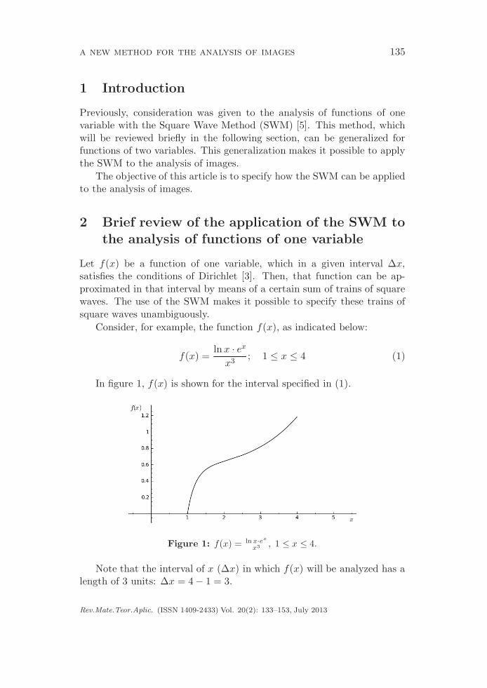
Consider, for example, the function f(x), as indicated below:

f(x) =ln x · ex

x3; 1 ≤ x ≤ 4 (1)

In figure 1, f(x) is shown for the interval specified in (1).

Figure 1: f(x) = ln x·ex

x3 , 1 ≤ x ≤ 4.

Note that the interval of x (∆x) in which f(x) will be analyzed has alength of 3 units: ∆x = 4− 1 = 3.



First, an explanation will be given about how to proceed if one wantsto obtain an approximation to f(x), in the interval ∆x specified in (1),

made up of the sum of 6 trains of square waves. The interval ∆x is thendivided into a number of sub-intervals – of equal length – which is the

same as the number of the trains of square waves. In this case, therewill be 6 sub-intervals. The approximation to f(x) to be obtained in the

interval ∆x will be the sum of 6 trains of square waves: S1, S2, S3, S4,S5, and S6. The first of the trains of square waves is denominated S1, thesecond S2, and so on.

Each of these trains of waves Si, for i = 1, 2, 3, 4, 5 and 6, will be

characterized by a certain “spatial frequency” fi; that is, the number ofwaves in the train of square waves considered which is contained in the

unit of length, and a certain amplitude.

For the case considered here, a description will be provided below of

how the amplitudes corresponding to the different trains of square wavesare determined (see figure 2).

Figure 2: How to apply the SWM to the analysis of the function represented infigure 1 (see indications in text).

The vertical arrow pointing down at the right of figure 2 indicates how

to add the terms corresponding to each one of the 6 sub-intervals of ∆x.Thus, to obtain the values of the amplitudes corresponding to S1, S2, S3,

S4, S5 and S6, the following system of linear algebraic equations must besolved:



A1 + A2 + A3 + A4 + A5 + A6 = V1

A1 + A2 + A3 + A4 + A5 − A6 = V2

A1 + A2 + A3 + A4 − A5 + A6 = V3

A1 + A2 + A3 − A4 − A5 − A6 = V4

A1 + A2 − A3 − A4 + A5 + A6 = V5

A1 − A2 − A3 − A4 + A5 − A6 = V6.

(2)

In the preceding system of linear algebraic equations (2), V1, V2, V3,V4, V5, and V6 are the values for f(x) as specified in (1) at the mid-

points of the first, second, third, fourth, fifth, and sixth sub-intervals,respectively, of the interval ∆x in which f(x) is analyzed. It follows thatthe values Vi, for i = 1, 2, 3, 4, 5 and 6, can be computed given that f(x)

has been specified in (1). These values are: V1 = 0.398769931690279, V2 =0.600884713383228, V3 = 0.675458253887002, V4 = 0.760888387081983,

V5 = 0.885510437891641, and V6 = 1.06576570701653.The six unknowns of the system of equations specified in (2) are A1,

A2, A3, A4, A5, and A6. |Ai| refers to the “amplitude” of the train ofsquare waves Si for i = 1, 2, . . . , 6. The (constant) value of each positive

square semi-wave of the train of square waves Si is |Ai|, and the (constant)value of each negative square semi-wave of that Si is −|Ai|. For the case

discussed here, in which ∆x was divided into 6 equal sub-intervals, thespatial frequencies corresponding to the different trains of waves are thefollowing:

f1 =1

2∆x

(

6

6 − 1 + 1

)

=1

2∆x

(

6

6

)

=1

6

f2 =1

2∆x

(

6

6 − 2 + 1

)

=1

2∆x

(

6

5

)

=1

5

f3 =1

2∆x

(

6

6 − 3 + 1

)

=1

2∆x

(

6

4

)

=1

4

f4 =1

2∆x

(

6

6 − 4 + 1

)

=1

2∆x

(

6

3

)

=1

3

f5 =1

2∆x

(

6

6 − 5 + 1

)

=1

2∆x

(

6

2

)

=1

2

f6 =1

2∆x

(

6

6 − 6 + 1

)

=1

2∆x

(

6

1

)

=1

1= 1.

In general, if the spatial interval ∆x – whose length, of course, maybe different from 3 – is divided into n equal sub-intervals, the spatial



frequencies corresponding to the different n trains of square waves are asfollows:

fi =1

2∆x

(

n

n − i + 1

)

; i = 1, 2, . . . , n. (3)

It can be useful to take interval ∆x as a unit of length. Therefore, thevalues obtained for the spatial frequencies of the diverse trains of square

waves are:

f1 =1

2

(

6

6

)

=1

2f2 =

1

2

(

6

5

)

=3

5

f3 =1

2

(

6

4

)

=3

4f4 =

1

2

(

6

3

)

= 1

f5 =1

2

(

6

2

)

=3

2f6 =

1

2

(

6

1

)

= 3.

The accuracy of the preceding equations may be checked by consultingfigure 2. Thus, half of the square wave S1, for example, occupies the new

unit of length ∆x, for f1 = 12 ; one square wave of S4 occupies ∆x, for

f4 = 1; three square waves of S6 occupy ∆x, for f6 = 3; etc.

If ∆x is taken as the unit of length, and if it is admitted that ∆x isdivided into n sub-intervals, the general expression for the frequencies of

trains of square waves S1, S2, . . . , Sn is as follows:

fi =1

2

(

n

n − i + 1

)

; i = 1, 2, . . . , n. (4)

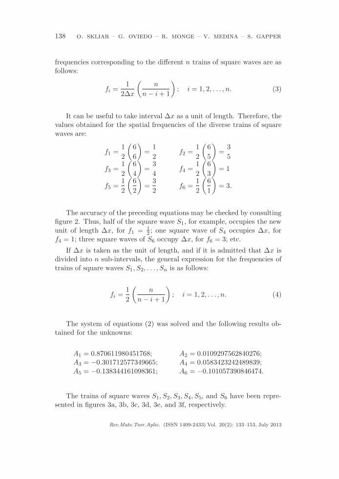
The system of equations (2) was solved and the following results ob-tained for the unknowns:

A1 = 0.870611980451768; A2 = 0.0109297562840276;A3 = −0.301712577349665; A4 = 0.0583423242489839;

A5 = −0.138344161098361; A6 = −0.101057390846474.

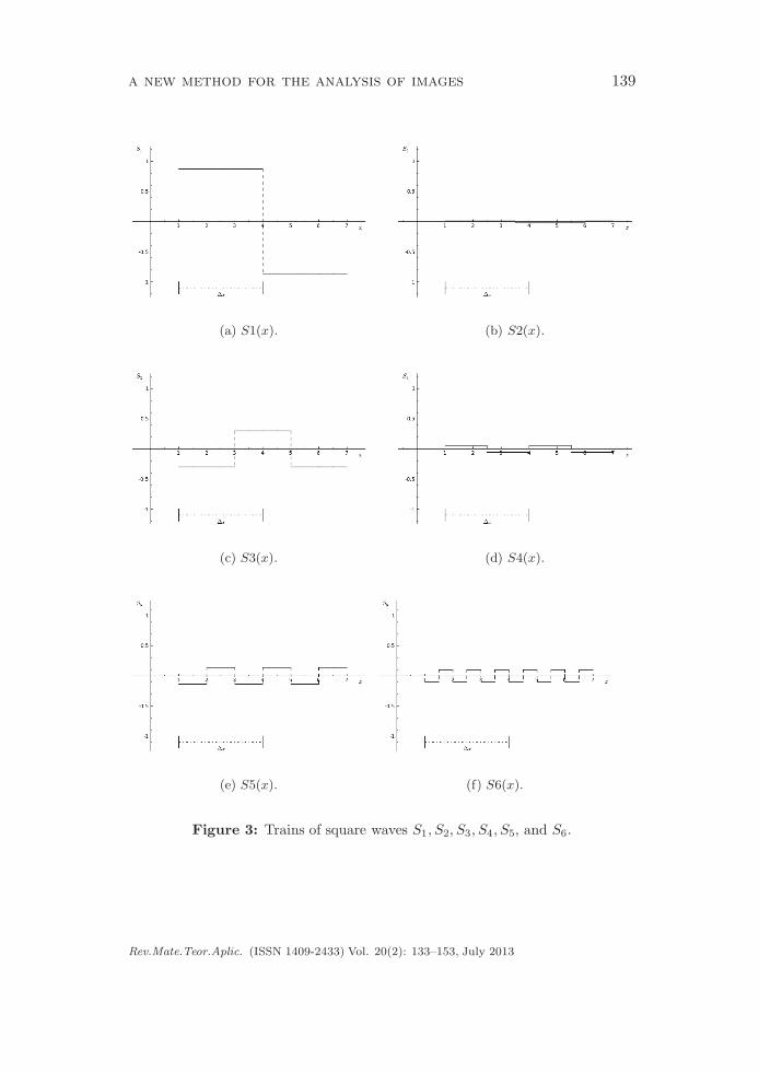
The trains of square waves S1, S2, S3, S4, S5, and S6 have been repre-sented in figures 3a, 3b, 3c, 3d, 3e, and 3f, respectively.



(a) S1(x). (b) S2(x).

(c) S3(x). (d) S4(x).

(e) S5(x). (f) S6(x).

Figure 3: Trains of square waves S1, S2, S3, S4, S5, and S6.



The approximation obtained for f(x) (as specified in (1), in interval∆x, by adding the six trains of square waves) has been displayed in fig-

ure 4.

Figure 4: Approximation to f(x), specified in (1) by

6∑

i=1

Si; f(x) is indicated

by a solid line.

If one wants to achieve, in interval ∆x, by adding the trains of square

waves, a better approximation to f(x), then ∆x should be divided into alarger number of equal sub-intervals. The larger the number of these sub-intervals, the better the approximation. Thus, for example, the approxi-

mation to f(x) that can be achieved if ∆x is divided into 18 sub-intervalsof equal length, is shown in figure 5. In this case, it is clear that 18 trains

of square waves were added up.The SWM cannot be considered a branch of Fourier Analysis; that is,

the trains of square waves Si, for i = 1, 2, . . . , n, do not make up a systemof orthogonal functions.

3 Characterization of the application of the SWM

to the analysis of images

First of all, the images to be analyzed must be digitized. It will be sup-

posed that the digitized images are made up of a set of pixels, and thatfor each pixel a certain level of gray may be established on the gray scale,



Figure 5: Approximation to f(x) specified in (1) by18∑

i=1

Si; f(x) is indicated by

a solid line.

ranging from black (0) to white (255). The possible numerical values in the

gray scale are as follows: 0, 1, 2, . . . , 255. In other words, these numericalvalues range from 0 (black) up to 255 (white), one unit at a time.

It may be admitted that the image to be analyzed occupies a rectan-

gular region, as usually occurs with pictures or photographs. (If the sidesof that rectangle are the same, as is acceptable, the rectangle is a square.)

To specify how the SWM is applied to the analysis of images, it will

be supposed initially that the region to be analyzed is made up of a smallnumber of pixels. (Later, this restriction will be eliminated.) Let there be

a rectangle such as that shown in figure 6.

Figure 6: An image made up of 6 pixels.



This rectangle is composed of two rows, each made up of 3 pixels.Likewise, it may be considered to be composed of three columns, each of

2 pixels. Of course, the total number of pixels in the rectangle is 6.Let it be admitted that the image to be analyzed is located in the area

∆x ·∆y. The interval ∆x has been divided into 3 equal sub-intervals. Theinterval ∆y has been divided into 2 equal sub-intervals.

In figure 7, a set of symbols has been added to the rectangle in figure6, both for the x-axis and for the y-axis. These symbols are of the typeshown in figure 2 (where the y-axis was not considered; therefore, symbols

such as B1, B2, and −B2 were unnecessary).

Figure 7: How to apply the SWM to the analysis of the image correspondingto figure 6.

In figures 6 and 7, the pixels have been named conventionally as mightbe expected, given the system of orthogonal Cartesian coordinates used

for reference.For each of the pixels in the rectangle considered, there is a linear

algebraic equation.A description will be provided below of how to find the linear algebraic

equation corresponding to pixel (3, 2). The same approach is used toobtain the equations corresponding to each of the other 5 pixels.

Note that the third sub-interval of ∆x and the second sub-intervalof ∆y correspond to pixel (3, 2). The symbols associated with the third

sub-interval of ∆x are: A1,−A2, and A3). The symbols associated withthe second sub-interval of ∆y are: B1, and −B2). Consideration will begiven first to the Cartesian product of the following sets: (A1,−A2, A3)

and (B1,−B2):

(A1,−A2, A3)× (B1,−B2) =

= ((A1, B1), (A1,−B2), (−A2, B1), (−A2,−B2), (A3, B1), (A3,−B2)) .



An operator O is introduced, which operates on each of the elementsbelonging to that Cartesian product. (Each one of these elements is an

ordered pair.) When that operator acts on an ordered pair, a term of acertain algebraic sum (to be specified) is obtained, to which a positive

sign must be attributed if the elements of the ordered pair have the samesigns, and a negative sign if the elements of the ordered pair have different

signs. The term obtained has two subscripts such that the first of them isthe same as the subscript of the first symbol of the ordered pair and thesecond subscript is the same as the subscript of the second symbol of the

ordered pair.

According to the explanation provided in the above paragraph, thefollowing results are obtained:

O(A1, B1) = C1,1

O(A1,−B2) = −C1,2

O(−A2, B1) = −C2,1

O(−A2,−B2) = C2,2

O(A3, B1) = C3,1

O(A3,−B2) = −C3,2.

(5)

The right-hand members of the above equalities are the terms men-tioned. If the algebraic sum of those terms is made equal to the numerical

value corresponding to the level of gray of pixel (3, 2), V3,2, the followinglinear algebraic equation is obtained for that pixel:

C1,1 − C1,2 − C2,1 + C2,2 + C3,1 − C3,2 = V3,2.

If the same procedure is applied for each of the other 5 pixels of therectangle, 5 more linear algebraic equations are obtained. Together with

the first one, they make up the following system of linear algebraic equa-tions:

C1,1 + C1,2 + C2,1 + C2,2 + C3,1 + C3,2 = V1,1

C1,1 − C1,2 + C2,1 − C2,2 + C3,1 − C3,2 = V1,2

C1,1 + C1,2 + C2,1 + C2,2 − C3,1 − C3,2 = V2,1

C1,1 − C1,2 + C2,1 − C2,2 − C3,1 + C3,2 = V2,2

C1,1 + C1,2 − C2,1 − C2,2 + C3,1 + C3,2 = V3,1

C1,1 − C1,2 − C2,1 + C2,2 + C3,1 − C3,2 = V3,2.

(6)

It is admitted that the values Vi,j (for i = 1, 2, 3; and j = 1, 2) areknown.



Figure 8: How to apply the SWM to the analysis of the image represented here,made up of 9 pixels.

Another example similar to that of figure 7 has been provided in figure

8 to show the system of linear algebraic equations obtained.

The system of linear algebraic equations obtained by applying theSWM to the image in figure 8 is as follows:

C1,1 + C1,2 + C1,3 + C2,1 + C2,2 + C2,3 + C3,1 + C3,2 + C3,3 = V1,1

C1,1 + C1,2 − C1,3 + C2,1 + C2,2 − C2,3 + C3,1 + C3,2 − C3,3 = V1,2

C1,1 − C1,2 + C1,3 + C2,1 − C2,2 + C2,3 + C3,1 − C3,2 + C3,3 = V1,3

C1,1 + C1,2 + C1,3 + C2,1 + C2,2 + C2,3 − C3,1 − C3,2 − C3,3 = V2,1

C1,1 + C1,2 − C1,3 + C2,1 + C2,2 − C2,3 − C3,1 − C3,2 + C3,3 = V2,2

C1,1 − C1,2 + C1,3 + C2,1 − C2,2 + C2,3 − C3,1 + C3,2 − C3,3 = V2,3

C1,1 + C1,2 + C1,3 − C2,1 − C2,2 − C2,3 + C3,1 + C3,2 + C3,3 = V3,1

C1,1 + C1,2 − C1,3 − C2,1 − C2,2 + C2,3 + C3,1 + C3,2 − C3,3 = V3,2

C1,1 − C1,2 + C1,3 − C2,1 + C2,2 − C2,3 + C3,1 − C3,2 + C3,3 = V3,3.

(7)



4 Application of the SWM to an image – a digi-

tized photograph of the Taj Mahal – composed

of 786,432 Pixels

The digitized image to be analyzed is displayed in figure 9.

Figure 9: Image of the Taj Mahal.

The image in figure 9 is made up of 786,432 pixels. Each row of the

image contains 1,024 pixels and each column 768 pixels.

If the SWM were applied directly to the analysis of the image in thefigure, a system of 786,432 linear algebraic equations with that same num-

ber of unknowns would have to be solved. That task would exceed theoperational capacity of the computer used for this purpose. Therefore, itwas necessary to divide the image into 768 sections. Each of these parts is

a square made up of 1,024 pixels. In other words, each square sub-imageobtained by dividing the image in figure 9, may be considered to be made

up of 32 rows, each with 32 pixels (or 32 columns, each with 32 pixelsalso). To conduct the analysis using the SWM for every sub-image means

solving a system of 1,024 linear algebraic equations, and that was feasibleusing the technical resources available.

Using the SWM, the analysis was carried out for all of the sub-imagesmentioned above. Thus, for each sub-image, it was possible to obtain



1,024 terms: Ci,j ; i = 1, 2, 3, . . . , 32; j = 1, 2, 3, . . . , 32. Once those termsare computed, it is feasible to obtain, for each pixel of each sub-image,

the corresponding algebraic sum whose value is made equal to the level ofgray of that pixel.

Given the characteristics provided for the image (in figure 9) to be an-

alyzed and the sub-images into which it was divided, it may be consideredthat this image is made up of 24 rows of sub-images, or 32 columns of

sub-images. Each sub-image belongs to only one of the 24 rows and toonly one of the 32 columns.

What is referred to here as “approximation (m, n) – Im,n” (1 ≤ m ≤

32 and 1 ≤ n ≤ 32), to the digitized image analyzed will be specifiedbelow. Suppose, for example, that one wants to obtain I7,24 for the image

analyzed. For this purpose, the sum is obtained algebraically for eachpixel of all of the sub-images, only for those terms Ci,j such that 1 ≤ i ≤ 7and 1 ≤ j ≤ 24. Therefore, the terms, C5,11, C3,24, and C4,2, for instance,

would be terms of the algebraic sum corresponding to each pixel. However,terms such as C5,28 (note that 28 > 24), C27,32 (note that 27 > 7 and

32 > 24), and C9,24 (note that 9 > 7) are not included in the algebraicsum corresponding to each pixel.

It will be admitted that when both subscripts are the same for an

approximation of the type discussed (such as I17,17), one subscript suf-fices; in this case, I17. With this convention, it is evident that I32 is the

same as the image analyzed. (Hence, that image is one of the sub-imagesmentioned above.)

From that image, I12, I16, I120, I24, I28, I29, I30, I31, and I32 are

displayed in figures 10a, 10b, 10c, 10d, 10e, 10f, 10g, 10h, and 10i, respec-tively. Note that I32 coincides with that image, as shown in figure 9. (Of

course, when stating that any Ii, for i = 1, 2, . . . , 32, is obtained for theimage in figure 9, what is meant is that Ii is obtained for each of the 768

sub-images into which the image was divided.)

Reference may be made to each sub-image in the following way: Sup-pose that the rows of the sub-images are numbered from bottom up, from

1 to 24, and that the columns of the sub-images are numbered from leftto right, from 1 to 32. Given that each sub-image belongs to only one rowof sub-images and to only one column of sub-images, each sub-image can

be unambiguously specified by indicating the row and column to which itbelongs. Thus, for example, sub-image (8, 27) is that belonging to column

8 and row 27, according to the convention that the first element of theordered pair (8, 27) refers to the column and the second to the row.



(a) Approximation 12 (I12). (b) Approximation 16 (I16).

(c) Approximation 20 (I20). (d) Approximation 24 (I24).

(e) Approximation 28 (I28). (f) Approximation 29 (I29).

Figure 10: Different approximations to the image in figure 9.



(g) Approximation 30 (I30). (h) Approximation 31 (I31).

(i) Approximation 32 (I32).

Figure 10: Different approximations to the image in figure 9 (Cont.).

The contribution of each term Ci,j, for i = 1, 2, . . . , 32; andj = 1, 2, . . . , 32, to the value of the level of gray of each pixel in each

row and in each column of each sub-image can be positive, negative, orzero. If for any sub-image of those considered, the contribution of any

term to the value of the level of gray of each pixel in any row or columnis graphed, what is obtained is the representation of part of a train ofsquare waves. To specify each train of square waves, a notation will be

introduced and it will be illustrated by two examples.Suppose that one wants to graph the contribution of C7,24 to each pixel

in row 18 of sub-image (15, 23). Reference will be made to the train ofsquare waves to which the graph belongs, in the following way:

S ((15, 23), C7,24, ( , 18)) .



It was shown that the train of square waves considered is a functionof an ordered set of three elements. The first element is the ordered

pair, (15,23), which specifies the sub-image to which that particular rowbelongs. The second element indicates the term considered: C7,24. The

third element ( , 18) is a “pseudo-ordered-pair”, whose first element ismissing, and whose second element refers to row 18.

Here is another example: S((7, 10), C15,30, (12, )) is the train of squa-re waves representing the contribution of element C15,30 to each pixel incolumn 12 of the sub-image (7, 10). In figures 11a and 11b, this has been

graphed in trains of square waves.To determine the spatial frequency of any train of square waves of the

type represented in figure 11a and 11b, how each term Ci,j was obtainedshould be kept in mind (see (5)). If the contribution of that term to a

row is taken into account, the first subscript of Ci,j must be consideredand formula (3) applied (or (4), according to which length is chosen as

the unit of length: the length of a side of a pixel or the length of ∆x,respectively).

Suppose that one wishes to determine the spatial frequency ofS((15, 23), C7,24, ( , 18)) using first the length of one side of a pixel (whichmay be any side, since it is accepted that pixels are square) as the unit

of length. Given that the train of square waves considered corresponds tothe contribution of the term C7,24 to a row (row 18), the first subscript

(7) of that term must be taken into account. Given that in this casethe image analyzed is one of the sub-images used (one square such that

∆x = ∆y = 32), upon applying (3), the spatial frequency for that trainof square waves is obtained:

f7 =1

2∆x

(

32

32− 7 + 1

)

=1

2

(

1

26

)

=1

52.

If, on the other hand, ∆x is the unit of length used to calculate the

corresponding frequency, by applying (4), the following result is obtained:

f7 =1

2

(

32

26

)

=16

26=

8

13.



(a) [S((15, 23), C7,24, ( , 18)).

(b) S((7, 10), C15,30 , (12, )).

Figure 11: Trains of square waves specified in (a) and (b).



Suppose that one wishes to determine the spatial frequency ofS((7, 10), C15,30, (12, )) using, first of all, the length of one side of a

pixel as a unit of length. Given that the train of square waves consideredcorresponds to the contribution of term C15,30 to a column (column 12),

the second subscript (30) of that term should be taken into account. By(3), the following result is obtained:

f30 =1

2∆x

(

32

32 − 30 + 1

)

=1

2

(

1

3

)

=1

6.

If, however, ∆y is chosen as the unit of length, and it is recalled thatfor the case considered, ∆x = ∆y = 32, by applying (4), the following

result is obtained:

f30 =1

2

(

32

32− 30 + 1

)

=16

3.

5 Discussion and perspectives

5.1 Discussion

Analyzing any entity implies determining its components, according tocertain criteria which must be defined. Analyzing a function of one vari-

able (f(x)) within a specific interval (∆x) using the SWM, one can de-termine the trains of square waves once the function in that interval is

digitized; i.e., the components of the entity considered, according to thecriterion established by the method.

In this article the generalization of the SWM was presented for the

analysis of images.

In a given region when the SWM is applied to the analysis of an image,a digitized “version” of that image must first exist. Actually, the entity

analyzed is the digitized image.

According to the notion of digitized image used here, that image couldbe considered to be a function of two variables, which is digitized, or made

discrete, in a certain region.

The components that make up the digitized entity —the digitizedimage— are also, according to the criterion established by the SWM,

trains of square waves. Each row and each column of the digitized imagecan be reconstructed by adding up all of the trains of square waves cor-

responding to that particular row or column. The entities analyzed herewere actually sub-images of a given image. Each sub-image considered was



a square which could be thought to be made up of 32 rows of 32 pixelseach, or of 32 columns of 32 pixels each. Every row and every column of

that digitized sub-image con be reconstructed by adding up 1,024 trainsof square waves. Each one of these trains of square waves can be unam-

biguously determined by the SWM procedures specified. Reconstructingall the rows or all the columns of a digitized sub-image is equivalent to

obtaining once again the value of the level of gray of each pixel in thegiven sub-image.

The SWM is a systematic method for analyzing any digitized imageof the type considered, such as that of any digital photograph displayedusing a gray scale.

Regarding the approach described, one limitation (pragmatically irrel-evant but theoretically important) is the following: No proof was presented

here of the existence and uniqueness of the solution of systems of linearalgebraic equations such as (5).

From the computational viewpoint, applying the SWM to the analysisof images is simple and direct: Adequate software for the solution of

algebraic linear equations already exists.

5.2 Perspectives

The generalization of the approach presented for digitized color images isimmediate. The color corresponding to each pixel of the color image is

achieved by the composition of three levels of color: those correspondingto three primary colors. Hence, any color image can be “decomposed”

into three images: the first is done with one of the primary colors, thesecond with another of them and the third with the remaining primary

color. Therefore, each of these three images may be analyzed using themethod described here.

The level of gray for each of the pixels mentioned is achieved by com-posing the same levels of color for each of the three primary colors. Thus,for example, if one of the three primary colors is (PC)1, another is (PC)2,

and the other (PC)3, gray level 57 is obtained by composing level 57 of(PC)1, (PC)2, and (PC)3. For this reason, for images made up of dif-

ferent levels of gray, it is not necessary to carry out three processes ofanalysis, one for each of the three color images mentioned. Those three

analyses would lead to the same numerical results.

The use of the SWM for the analysis of color images will be discussed

in further detail elsewhere.

Three other issues will also be addressed:



a. applying the SWM to the analysis of functions of n variables –f(x1, x2, . . . , xn); this generalization would be useful for providing

a geometric interpretation of the SWM applied to functions of anynumber (n = 1, 2, . . . , n) of variables;

b. the role that the SWM can have in the numeric solution of differ-ential equations of interest in mathematical physics (e.g.: Laplace’sequation) with quite varied boundary conditions; and

c. certain applications of the SWM to the analysis of signals and imageswhich are of interest in the field of biomedicine.

To the authors’ best knowledge, the method presented here for image

analysis has not been used previously. No references were found on thetopic in the literature reviewed regarding image analysis and processing.

In the vast amount of references, very diverse issues are addressed, suchas image segmentation, image dilation, image erosion, image thresholding,image enhancement and image compression. A preliminary introduction

to these topics may be found, for example, in [1], [6], [2] and [4]. As theSWM and its applications continue to be developed, it will be possible to

determine whether it will be a significant contribution, complementary tothe diverse methods existing for the analysis of signals and images.

References

[1] O’Gorman, L.; Sammon, M. J.; Seul, M. (2008) Practical Algorithms

for Image Analysis. Cambridge University Press, Cambridge.

[2] Petrou, M.; Petrou, C. (2010) Image Processing: The Fundamentals.

2nd ed. John Wiley and Sons, West Sussex, U.K.

[3] Riley, K.F.; Hobson, M.P.; Bence, S.J. (2006) Mathematical Methods

for Physics and Engineering. Cambridge University Press, Cambridge.

[4] Russ, J.C. (2011) The Image Processing Handbook, 6th ed. CRC Press,Boca Raton, FL.

[5] Skliar, O.; Medina, V.; Monge, R. E. (2008) “A new method for the

analysis of signals: the square wave method”, Revista de Matematica.

Teorıa y Aplicaciones 15(2): 109–129.

[6] Sonka, M.; Hlavac, V.; Boyle, R. (2007) Image Processing, Analysis

and Machine Vision, 3rd ed. CL-Engineering, Milwaukee, WI.


A New Method for the Analysis of Images: The Square Wave Method

Documents

Transcript of A New Method for the Analysis of Images: The Square Wave Method