INSTITUTE OF PHYSICS PUBLISHING JOURNAL OF PHYSICS B: ATOMIC, MOLECULAR AND OPTICAL PHYSICS

J. Phys. B: At. Mol. Opt. Phys. 39 (2006) 4379–4392 doi:10.1088/0953-4075/39/21/004

A wave packet method for treating nuclear dynamicson complex potentials

S Taioli and J Tennyson

Department of Physics and Astronomy, University College London, Gower St, London WC1E6BT, UK

Received 27 April 2006, in final form 25 August 2006Published 17 October 2006Online at stacks.iop.org/JPhysB/39/4379

AbstractA general time-dependent description of the dissociative attachment of atriatomic molecule is presented. The approach presented works within theFeshbach projection operator formalism and gives an algorithm for solving thenuclear motion problem which reduces the computational effort required.The method uses a complex potential energy surface to characterize theformation and decay of resonances as modified by the coupling to the nuclearmotion which are treated using multidimensional complex wave packets.A basis-independent wave packet method is developed and used to treatthe propagation of a wave packet on a complex three-dimensional potentialappropriate for resonance states of the water anion. A complete derivationof the system of linear equations used in the time iteration is presented. Themethod can be applied to resonant vibrational excitation, for which the electronimpact vibrational excitation of water is considered.

1. Introduction

Calculations on scattering processes have been traditionally performed in the frameworkof energy domain quantum mechanics and for molecules with just one degree of freedom(Bardsley 1966, Morgan et al 1990). In the last few years advances in computer memoryand development in computation techniques have made it possible to numerically solve thetime-dependent Schrodinger equation (Balakrishnan et al 1997, Gertitschke and Domcke1993, Schneider et al 2006) for a variety of processes including photodissociation (Kulanderet al 1990), atom–molecule reactive collisions (Zhang and Zhang 1994), Bose–Einsteincondensation (BEC) (Inguscio et al 1999), resonant dissociative collisions (dissociativerecombination (Orel and Kulander 1993) and electron attachment (Haxton et al 2004b))and vibrational excitation via resonance (Schulz 1973). The evolution in time is the mostintuitive and appealing frame for dynamics for at least two different reasons. First, the useof the laws of quantum mechanics in time-dependent approach is analogous to the classical

0953-4075/06/214379+14$30.00 © 2006 IOP Publishing Ltd Printed in the UK 4379

4380 S Taioli and J Tennyson

mechanics description. It gives an intuitive insight into the dynamics, often hidden in time-independent calculations, because one can view snapshots of the wave packets by simplyplotting probability densities at various stages of the time evolution and hence obtain a feel forthe dynamics. Indeed, by studying wave packets one touches the border between classical andquantum behaviour as it is well known that a wave packet must be associated with a bunch ofdeterministic classical trajectories. Second, the Schrodinger equation is first order in time andthus the scattering problem can be solved for a variety of energies with just one wave packetrun by performing a simple Fourier transform. These results can then be directly compared tothe experiment, where time resolution of the interacting systems can be difficult to achieve.

Time-dependent methods can be used to compute both the dynamics of atoms boundin a molecule and the dynamics of dissociation following an excitation by an impingingparticle. Whereas our understanding of non-dissociative collisions has advanced greatlyrecently, largely due to the development of theories capable of treating correctly the strongforward peak of most such cross sections, less is known about collisions which dissociate themolecule. Impact dissociation is important for astrophysics, radiation damage of living tissueand in the ionosphere. Dissociative electron–molecule collisions such as dissociative electronattachment (DEA), which competes with vibrational excitation (VE), cause strand breaks inDNA and, as a result of fragmentation or recombination of the molecules, produce chemicallyreactive radicals (Boudaiffa et al 2000, Pimblott and LaVerne 2002). It is now widely acceptedthat such collisions often proceed via a resonant state in which the impinging particle loses itskinetic energy for a period of time of the same order as the vibrational motion and can decayby a variety of different paths.

While the dynamics of resonant collisions in the simple case of a one-dimensionalpotential, such as electron collision with diatomic molecules (Morgan 1986, Hazi et al 1981,Robicheaux 1991, Brems et al 2002) seems to be well established, the best general methodfor treating fully multidimensional nuclear motion is still the subject of discussion. In generalmultidimensional problems have different reaction paths which yield different products, eachwith different probability amplitudes. This means that quantal effects due to sharing energybetween electronic and nuclear motion have to be treated in all the nuclear degrees of freedomto correctly model the vibrations and dissociation of the molecule. Alternative computationalprocedures are represented by the path-integral approach of Feynman (1981) and Feynmanand Hibbs (1965), the multiconfigurational time-dependent Hartree representation of thewavefunctions (MCTDH), developed by Beck et al (2000), and the spectral method dueto Feit and Fleck (1982).

All have been used to develop approximation methods for treating both local and non-localdynamics (Winterstetter and Domcke 1993). The path-integral approach, which is motivatedby the linear scaling with the number of degrees of freedom if one uses the harmonic oscillatorapproximation for the vibrational modes, suffers problems with choosing suitable weights forthe electronic paths and from the need to introduce a discrete basis at every intermediate time.The MCTDH approach makes use of the time-dependent representation of the nuclear wavepacket as a linear combination of single-particle functions: the greater the number of terms, themore precise is the calculation. It has been used to treat the dissociative attachment of water inall three vibrational degrees of freedom using a method tailored ad hoc to this system (Haxtonet al 2004b). The spectral method has been used (Kazansky and Sergeeva 1994, Kazansky1995) for calculating both inelastic and DEA cross sections of slow electrons with carbondioxide. In such a case the solution of the time-dependent Schrodinger equation was obtainedusing the split time propagation method where the propagation of the wave packet is splitinto a free-particle propagation over a half-time, a whole time propagation for the potentialpart and a third free particle action step to end the propagation. This method, as the authors

A wave packet method for treating nuclear dynamics on complex potentials 4381

acknowledge, relies on the existence of the fast Fourier transform algorithm (FFT) and on theexplicit independence of the kinetic energy from the spatial coordinates. Furthermore thismethod appears unsuitable for joining with a Chebyshev propagation scheme. Our methodhas a different prospective: it actively uses Chebyshev propagation and can be used with orwithout an FFT algorithm.

The purpose of this paper is to present a new method, both theoretical and computational,for calculating the dynamics subsequent to excitation of a polyatomic molecule. This methodstill retains the time-dependent view but, in contrast to standard methods for solving theSchrodinger equation which are basis dependent, uses a grid Hamiltonian. The method usesa complex potential to represent the resonance state, can take into account all nuclear degreesof freedom and can treat both DEA and resonant VE. The algorithm we present transformsthe decaying partial differential equation to a set of coupled linear equations for the real andimaginary parts of the wave packet. It gives a rigorous treatment of the non-separability intime between the real and imaginary parts due to the decay.

This distinguishes the method and the computation procedures from some employedpreviously (Kulander et al 1990). The coupled linear equations, as explained below, aresolved iteratively, using large time steps due to an efficient Chebyshev expansion scheme.This enables us to handle the exponential growth in the computational effort with thenumber of degrees of freedom by a combination of minor improvements in the theory andmajor changes to the computational procedure. In particular we choose different suitablecoordinate systems, and consequently grids, as well as representations of the Hamiltonianoperator.

We limit ourselves to the discussion of nuclear excitation and dissociation processesin a sample triatomic molecule, water. However we believe that the methods we presentare sufficiently general to be applied to the analysis and interpretation of different physicalproblems, such as resonances in tetratomic molecules or processes involving the interactionbetween matter and light.

2. Method

The calculation of electron–molecule impacts resulting in dissociative electron attachment(DEA) or resonant vibrational excitation (VE) splits naturally into two parts: the firstcomprising electron dynamics and the second nuclear motion dynamics. Our goal is tocombine accurate first principles electronic motion calculations with a wave packet treatmentof the nuclear dynamics with multiple nuclear degrees of freedom. The computationof the complex potential surfaces of the combined electron–molecule complex is not thesubject of this paper: the electronic motion can be studied using standard methods such asab initio complex Kohn variational calculations (McCurdy and Rescigno 1989) or themolecular R-matrix method (Burke and Berrington 1993). Fixed-nuclei calculations areused to obtain complex potential energy surfaces. As result of the collision the molecule canbe excited to one or more short-lived resonant states embedded in the continuum which decaywith time. Excitation of such quasi-bound resonances results mainly in two different physicalprocesses: vibrational excitation and dissociative attachment. In the former the molecule isleft in its electronic ground state but vibrationally excited; in the latter there must be sufficientenergy for a bond to be broken and the molecule follows a dissociative path. For the followinggeneral analysis it is not necessary to specify if we are dealing with a shape or a Feshbachresonance: we just assume a single complex electronic state which is discrete, as opposedto the continuum of states with which it interacts. Generalization to more than one distinctdiscrete state is straightforward.

4382 S Taioli and J Tennyson

AB

C

r R

G

γ

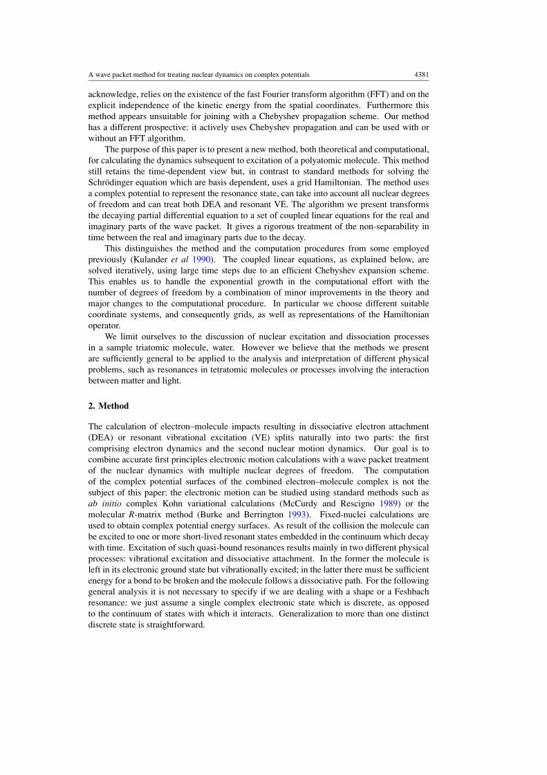
Figure 1. Body-fixed Jacobi coordinate system: A, B, C represent atoms. The coordinates aregiven by r = B − C, R = G − A and the angle γ = ˆAGC. G is the centre of mass of BC.

2.1. The nuclear motion: the model Hamiltonian

The time-dependent projection operator formulation has been described in detail elsewhere(Gertitschke and Domcke 1993), so here we just give a brief outline. For an isolated resonancewe assume that the Hilbert space of the electronic configurations is spanned by a simple L2

function |φd〉. This assumption is clearly based on the Born–Oppenheimer approximation.Partitioning the total wavefunction into resonant and non-resonant components defines twoprojectors (Feshbach 1962)

Q = |φd〉〈φd |, P = 1 − Q. (1)

One can reduce the treatment of nuclear dynamics in a complex energy-dependent and non-local potential to a local complex potential, which is known as the Markov approximation forthe decay dynamics (Cederbaum and Domcke 1981). Projecting out the electronic motion,we are left with the equation of motion of the nuclei

i∂�d(R, r, γ, t)

∂t=

[TN(r, R, γ ) + Vd(r, R, γ ) − i

2�L(r, R, γ )

]�d(R, r, γ, t) (2)

where TN is the nuclear kinetic energy operator, Vd is the potential energy of the discreteelectronic state and

�L(r, R, γ,Eres) = �L(r, R, γ ) = 2π

∫d�k|Vdkf

(r, R, γ )|2 (3)

in which �L(r, R, γ ) is the width taken at the resonance energy and the discrete–continuumcoupling enters via the ‘exit amplitude’ Vdkf

.

2.2. Jacobi coordinate system

To treat the dissociative and vibrational problem, we use Jacobi coordinates. A sketch of thiscoordinate system is presented in figure 1. In scattering coordinates r represents the diatomdistance between atom B and atom C, and R the separation of atom A from the diatom centreof mass. The angle between r and R is γ .

A formal definition of the rotational–vibrational wave packet in body-fixed Jacobicoordinates is

�JM(R, r, γ, α, β, ζ ) =J∑

K=−J

DJMK(α, β, ζ )

�JMK (R, r, γ )

Rr(4)

where DJMK(α, β, ζ ) is the set of normalized Wigner rotation matrices (Wigner 1939), J is

the total angular momentum, and M is the z component of the total angular momentum in thelaboratory frame. In equation (4), K is the projection of the total angular momentum on the

A wave packet method for treating nuclear dynamics on complex potentials 4383

body-fixed z axis which we take as R ≡ z, and (α, β, ζ ) are the three Euler angles whichorient the body frame to the laboratory frame. The left-hand side of equation (4) is thus in thelaboratory frame and the right-hand side is in the body frame.

3. Solution of the equation of motion

A single nuclear dynamics problem, defined by equation (2), is considered for DEA and VE.It is solved in three different steps: wave packet creation, wave packet evolution and extractionof the observables of interest.

3.1. The initial condition

To begin the propagation of the wave packet, we need to introduce an initial condition thatsets the total energy as a sum of the collision energy of the impinging particle Etrans and theinitial vibrational energy of the triatomic molecule εν :

E = Etrans + εν = k2

2+ εν. (5)

The best choice for the initial condition for DEA and VE calculations is (Domcke 1991)

|�d(0)〉 = Vdki |v〉 (6)

where ki denotes the momentum of the incoming particle, |v〉 the initial vibrational state ofthe molecule and

Vdki = 〈ki(t)|V |ψd〉 =√

�/(2π) (7)

is the ‘entry amplitude’. This is known as ‘vertical transition’ approximation and definesthe initial wave packet which sets the clock at t = 0 for the dynamical evolution of thesystem.

3.2. Evolution in time

Equation (2) can be formally solved by introducing the operator

U = exp

(− i

h

∫ˆH(t) dt

), (8)

which gives the state of a system at a later time. In our case the total Hamiltonian,equation (2), is not Hermitian because the wave packet can bifurcate and decay to the groundstate:

HT = HR + iHc = TN + Vd − i�

2. (9)

The real part of the body frame Hamiltonian in Jacobi coordinates is written (Tennyson andSutcliffe 1982), in atomic units:

HR = − 1

2µR

∂2

∂R2− 1

2µr

∂2

∂r2−

[1

2µRR2+

1

2µrr2

]j 2

− 1

2µRR2

[J (J + 1) − 2K2 + CJ

K,K−1

(− ∂

∂γ+ K cot(γ )

)

+ CJK,K+1

(∂

∂γ+ K cot(γ )

)]+ Vd(R, r, γ ) (10)

where K is the projection of the total angular momentum on the R axis and

4384 S Taioli and J Tennyson

j 2 = 1

sin γ

∂

∂γsin γ

∂

∂γ− K2 cosec2 γ (11)

CJK,K±1 = [J (J + 1) − K(K ± 1)]1/2 (12)

and the appropriate reduced masses are

µR = mA(mB + mC)

mA + mB + mC

, µr = mBmC

mB + mC

(13)

and the atoms are defined by figure 1. Putting J = 0 means K is a good quantum number andthe wave packets are not coupled by the Coriolis terms. Previous calculations (Schulz 1973,Haxton et al 2004b) suggest that the rotational state of the triatomic has negligible effect onthe cross section for DEA and VE. The same is not true for different initial vibrational modesof the target.

The 3D Hamiltonian (equation (10)) is solved by successive time iteration (Balint-Kurtiet al 1998); the time evolution of the wave packet is governed by equation (2) for a givenpotential. A similar approach has been used in reactive scattering by Gray (1992) and Gray andBalint-Kurti (1998) for the propagation of real wave packets on real potential surfaces. Theseworkers were able to predict the evolution of an initial complex wave packet on a real surfaceby only propagating the real part. We cannot follow this approach, which halves the computertime and the memory, due to the complex potential. The presence of an electromagnetic fieldor consideration of spin would have the same effect on the Hamiltonian.

By dividing the time coordinate into two, one can split the problem into forward

�( �R, t + τ) = U(t + τ, t)�( �R, t) = exp−iHT τ

h�( �R, t)

= + exp−�τ

2h

[cos

(HRτ

h

)− i sin

(HRτ

h

)]�( �R, t) (14)

and backward propagation

�( �R, t − τ) = U(t − τ, t)�( �R, t) = exp+iHT τ

h�( �R, t)

= + exp+�τ

2h

[cos

(HRτ

h

)+ i sin

(HRτ

h

)]�( �R, t). (15)

Adding the right-hand side of the two previous equations one obtains

�( �R, t + τ) = −�( �R, t − τ) + 2

[cos

(HRτ

h

)cosh

(�τ

2h

)

+ i sin

(HRτ

h

)sinh

(�τ

2h

)]�( �R, t) (16)

�( �R, t + τ) = +�( �R, t − τ) − 2

[cos

(HRτ

h

)sinh

(�τ

2h

)

+ i sin

(HRτ

h

)cosh

(�τ

2h

)]�( �R, t) (17)

where the �R represents (R, r, γ ). This enables us to relate the wave packet at time t + τ to thatat time t and t − τ . Even if the iteration starts from a real initial wave packet, the imaginarypart in the above equations implies that the wave packet can become complex during thepropagation and our equations are coupled. To obtain an efficient computational method wemerged the benefits of a simple Chebyshev recursion relation (Tal-Ezer and Kosloff 1984),

A wave packet method for treating nuclear dynamics on complex potentials 4385

which is easy to implement but gives ‘time-step’ dependent results and is useful only for short-time propagators, with our ‘complex wave packet propagation’. for the real and imaginary partof the wave packet. Starting from the idea that the time coordinate does not enter in any of theobservables, we solve a mapped Schrodinger equation. To do this, we apply a transformationfrom real time to ‘mathematical time’, u and from the physical decay to the ‘mapped decay’,�s . The modified equation is

i∂|�(u)〉

∂u= [f (H) + ig(�)]|�(u)〉. (18)

The particular functions chosen for the transformation are those which simplify the iterativeform,

f (H) = −h

δcos−1(Hs) g(�) = −2h

δsinh−1

(�s

2

)(19)

where δ is the time step in mathematical time and we have introduced the normalizedHamiltonian Hs and width �s . The former is defined below as that whose eigenvaluesare within the interval [−1, 1], which is the domain of arccos; the latter is taken to be in thedomain of the sinh−1

�s = � − �av

��/2= cs� + ds (20)

where �� = �max − �min, �max and �min are the maximum and minimum values of the widthon the grid, respectively. �av is the average value of � and the scaling quantities cs and ds aredefined by the equation.

In the range of complex energies of interest the mapping is monotonic and thereforeinvertible. This is simple to see in the case of bound states but can usually be extended tocontinuum problems.

Taking the real part of equation (16) and the imaginary part of equation (17), we introducethe two real functions:

Q( �R, t) = RE[�], P ( �R, t) = IM[�]. (21)

In terms of these the recursion relations the wave packet become

Q(u + δ) = −Q(u − δ) + 2

√1 +

�2s

2HsQ(u) − 2

(�s

2

)√1 − Hs

2P(u) (22)

P(u + δ) = P(u − δ) + 2

(�s

2

)HsP (u) + 2

√1 +

(�s

2

)2√1 − Hs

2Q(u) (23)

where u = kδ is the mathematical time and k is the number of iterations requested forpropagating the wave packet.

As the initial wave packet is real for DEA and VE calculations, the first iteration isdifferent from subsequent iterations and the initial conditions are given by

Q(δ) = exp

(−�δ

2h

)HsQ(0) (24)

P(δ) = exp

(−�δ

2h

)√1 − Hs

2Q(0). (25)

The solution of the complete system as it is written in equations (22) and (23) iscomputationally slow (it scales as N3) but the complete Hamiltonian, which has to be read

4386 S Taioli and J Tennyson

‘on the fly’, can usually be stored in the memory. (Mandelshtam and Taylor 1995a, 1995b)proposed a new computational approach based on the iterative solution of simultaneous linearequations through a modified Chebyshev polynomial expansion of the root operator acting onthe wave packet. They introduced a scaled Hamiltonian

Hs = H − I(

�E2 + Vmin

)�E/2

= asH + bs (26)

where I is the identity operator, �E = Emax − Emin, Emax and Emin are the maximum andminimum eigenvalues of the Hamiltonian on the grid respectively, and the scaling quantitiesas and bs are defined by the equation. A rough estimate of the eigenvalues (one can alwaysthink that the spectral range is finite due to some L2 basis) can be obtained from

Emax = h2π2/2m(�x)2 + Vmin (27)

Emin = Vmin (28)

where Vmin is the minimum value of the potential; this gives for the scaled eigenvalues

Es = asE + bs. (29)

For dealing with a mapped decay, a transformation between the physical and mathematicaltime is necessary

t = has√1.0 − E2

s

u. (30)

This equation is obtained by linearizing and truncating the Taylor expansion of the firstequation of the mapping system, equation (19), at first order (Balint-Kurti et al 1998).

To evaluate the effect of the square root of the Hamiltonian on the wave packet we use aChebyshev series:

√1 − x2 = 2

π

[1 − 2

N∑k=1

T2k

4k2 − 1

](31)

where T2k(x) are the N Chebyshev polynomials of 2k-order (Abramowitz and Stegun 1972),calculated by the recursion formula

Tk+1(z) = 2zTk(z) − Tk−1(z) (32)

T0(z) = 1 (33)

T1(z) = z. (34)

3.3. Computational procedures

To minimize the computational time we need an efficient scheme of propagation which exploitsthe optimal representations for describing the action of each term of H on the wave packet.The choice of these different bases takes into account that the bottleneck of the calculationis the product between the representation of H itself and the wave packet. We chose threedifferent propagation schemes: fast Fourier transform (FFT) to treat the kinetic term, discretevariable representation (DVR) for the angular part and finite basis representation (FBR) forthe radial part of the potential. In FFT methods the grid is evenly spaced in the momentumspace and the quadrature scheme is comparable in accuracy to the DVR quadrature. The FFT

A wave packet method for treating nuclear dynamics on complex potentials 4387

scales as N log N , while a DVR scheme scales as N2, where N is the number of points in thegrid. The Fourier algorithm is an efficient technique which transforms a periodic sequencefrom the physical to spectral space defined as follows:

ψ(kj ) =√

L

N

[√2

N

∑i

ψ(xi) sinijπ

N

]= FFT[ψ(x)]. (35)

When applying this technique one pays the computational cost of dealing with non-localoperators, but it is possible to employ a less dense grid for a given accuracy. The angular partof the kinetic energy is treated using Legendre polynomials P K

j (x) (x = cos γ ) (Abramowitzand Stegun 1972). In treating the potential term we retain the radial FBR basis set, but for theangular part we use a DVR method.

It should be clear that, in the case of DEA, we are trying to represent the wave packetwhich is physically unbound on a finite grid and to calculate continuum quantities through adiscrete approximation. This could result in reflection of the wave packet back at the boundaryof the numerical grid, causing interference which destroys the real dynamics (Manolopoulos2002). Instead of enlarging the grid we solved the problem by employing a complex absorbingpotential (Migdley and Wang 2000, Muga et al 2004). As a consequence of using a formalismthat is easy to implement we pay the price of having a non-Hermitian Hamiltonian operatorand of losing some parts of the wave packet.

The complex absorbing potential causes the wave packet to be shaped by a Gaussianfunction (Gray 1992):

A(x) ={

1 z � zabs

exp[−Aabs(z − zabs)2] z > zabs

(36)

where zabs is the value of the radial coordinate where the wave packet begins to be absorbedand Aabs is an empirical coefficient which gives the strength of the absorption. This procedureswitches on the absorbing potential adiabatically, which does not greatly alter the wave packetshape in one single time step and gives stability to the numerical procedure. To estimatevibrational excitation we avoided the absorption in order to retain the entire wavefunction afterreaching the boundaries. We therefore perform an additional calculation which propagatesusing � = 0 which means the wave packet lives indefinitely on the resonance surface. Thedifference between the two calculated amplitudes is the total amount of wave packet whichdecays by autoionization of the resonance into the ground electronic state. As an example weconsider below the case of water excited to its stretching and bending vibrational fundamentalstates after an electron collision.

3.4. Observables

After propagating the wave packet one can extract the physical observables, such as the crosssections for DEA, VE, etc, using two approaches: asymptotic analysis and flux analysis. Thestarting point of the analysis in both methods is the value of the wave packet at a grid point(R = R∞) where dissociation has occurred. In a typical triatomic calculation, this meansthat the final diatom–atom products are formed. Results are comparable for each method;differences are simply due to the final quantities one wants to achieve: the scattering matrixin the first case, the T-matrix in the second one. We have chosen asymptotic analysis whichgives the scattering states directly without any need for transformation as the point where theanalysis is conducted is chosen to lie in the direction of the scattering products. A projectiononto the final diatomic states is needed to get wave packet coefficients as a function of time.

4388 S Taioli and J Tennyson

Energy-resolved observables can be obtained through a Fourier transform from the time to theenergy domain.

The analysis thus starts from the asymptotic value �(R∞, r, γ, u). Projection of such awave packet onto the final states of the diatom φjν(r) gives a set of time-dependent coefficientsAjν(u)

Ajν(u) =∫ ∞

0dr φjν(r)

∫dγP 0

j (γ )ψ(R∞, r, γ, u) (37)

where j and ν are the quantum numbers of the final rovibrational state of the diatom. Returningto the time-independent formal theory of scattering, where the dissociative wave packet hasan asymptotic behaviour analogous to an outgoing wave in the laboratory frame, we find

�JM(R, r, γ, α, β, ζ ) =J∑

K=−J

DJMK(α, β, ζ )

�JMK (R, r, γ )

Rr

R → ∞∑jν

Cjν(E)DJMK(α, β, ζ )

eikR−ijπ/2

Rrφν (38)

where φν are the vibrational wavefunctions of the diatom product, E is the total energy. Cjν(E)

are the partial wave amplitudes for the dissociative process. After projecting the asymptoticwavefunction onto φν the coefficients Cjν(E), Fjν(E) are the Fourier transform coefficientsfrom u of the real and imaginary parts of the Ajν(u) previously defined in equation (37).Mathematically:

Cjν(f (E)) = 1

2π

∫ ∞

0du exp(if (E)/h) Re[Ajν(u)] (39)

Fjν(g(E)) = 1

2π

∫ ∞

0du exp(ig(E)/h) Im[Ajν(u)]. (40)

The dissociative cross section resolved by quantum numbers of the final fragments can now beobtained from the asymptotic form of the solution of the time-dependent Schrodinger equation(Gertitschke and Domcke 1993) as

σ jν(E) =(∣∣∣∣df (E)

dE

∣∣∣∣2)

σ jν(f (E)) +

(∣∣∣∣dg(E)

dE

∣∣∣∣2)

σ jν(g(E))

= 2π2

E

κ

µR

(h2a2

s

δ(1 − E2

s

) ∣∣Cjν

(f

(Eνi

+ k2/2))∣∣2

+h2c2

s

δ(1 − �2

s

) ∣∣Fjν

(g(Eνi

+ k2/2))∣∣2

)

(41)

where κ is the relative nuclear momentum of the fragments and µR the reduced mass of thefragments.

That part of the vibrationally inelastic excitation which proceeds via the resonant processdiffers from the treatment of DEA only in the way the cross sections are obtained. Theasymptotic states of water in the adiabatic approximation are in this case the electronic groundstate and the vibrationally excited states; it is onto these states we have to consider theprojection of the evolved wave packet. In a similar fashion to equations (37) and (39), wedefine the quantities:

Aν(u) =∫ ∞

0dR dr

∫ 1

−1dγ φν(R, r, γ )P 0

j (γ )ψ(R, r, γ, u) (42)

A wave packet method for treating nuclear dynamics on complex potentials 4389

where, this time, φν(R, r, γ ) are the final vibrationally excited states of water, and

Cν(f (E)) = 1

2π

∫ ∞

0du exp(if (E)/h) Re[Aν(u)] (43)

Fν(g(E)) = 1

2π

∫ ∞

0du exp(ig(E)/h) Im[Aν(u)]. (44)

Following Domcke and Cederbaum (1977) and Narevicius and Moiseyev (1998), one canobtain for the cross section the expression:

σ ν(E) ∝ |E − Eν ||E|

1/2

(|Cν(f (Eν + k2/2))|2 + |Fν(g(Eν + k2/2))|2). (45)

We derive an expression for the normalized cross section within the framework of thelocal complex potential approximation which describes an impinging electron with energyE = Etrans which leaves the molecule in the vibrationally excited state ν and departs withenergy Etrans − Eν :

σ ν(E) =(∣∣∣∣df (E)

dE

∣∣∣∣2)

σ ν(f (E)) +

(∣∣∣∣dg(E)

dE

∣∣∣∣2)

σ ν(g(E))

= 2π3

E

(h2a2

s

δ(1 − E2

s

) |Cν(f (Eν + k2/2))|2 +h2c2

s

δ(1 − �2

s

) |Fν(g(Eν + k2/2))|2)

(46)

which gives the resonant contribution to the absolute vibrational excitation cross section.

4. Test calculations

To demonstrate our method we applied the theory to the study of both electron dissociativeattachment (DEA) and vibrational excitation (VE) of water. The X 2B1 resonance state ofthe water anion is known to be dissociative (Haxton et al 2004a) for a kinetic energy of theimpinging electron equal to 6.4 eV. There are two higher resonances at 8.4 eV and 11.2 eVwhich are also believed to be important for the dissociative electron attachment of water. Theprocesses under consideration are then

e− + H2O(vi) −→ H2O∗− −→ HO(v, j) + H− (47)

e− + H2O(vi) −→ H2O∗− −→ H2O(vf ) + e′− (48)

for the DEA and VE, respectively. In both cases we take the initial vibrational state, vi , to bethe vibrational ground state. In the case of DEA HO + H− are thought to be the most likelydirect products although energetically less favourable (Melton 1972).

Both calculations used the centrifugal sudden approximation, which means putting J = 0in the Hamiltonian. The total size of the grid chosen is (106×198×39) in r, R, γ , respectively,running in the range 0.6 to 6.9 for r and in the interval 0.1 to 11.98 for R; the angular grid ismade of 39 Gauss–Legendre quadrature points. Initial excitation Vdki was taken as the squareroot of �, the probability of excitation into the X 2B1 resonance state, at the equilibriumgeometry of water. The resonance width value we used is 0.004 eV. The DVR3D program(Tennyson et al 2004) was used to calculate wavefunctions for initial, vi , and final, vf , statesof water involved in the analysis. A separate program was written for projecting onto thedifferent vibrational states of OH.

4390 S Taioli and J Tennyson

0

0.05

0.1

0.15

0.2

0.25

3 4 5 6 7 8 9 10

Cro

ss S

ectio

n [s

quar

e bo

hr]

Electron kinetic energy [eV]

v=1v=2v=3v=4total

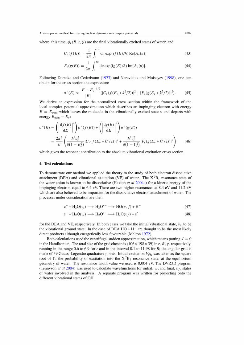
Figure 2. DEA cross section for H2O with increasing OH vibrational quantum number v, from leftto right. The top curve is the total cross section calculated as the sum of the underlying vibrationalspectra.

0

1

2

3

4

5

6

7

3 4 5 6 7 8 9 10

Tot

al C

ross

Sec

tion

[10-1

7 cm

2 ]

Electron kinetic energy [eV]

bend, calcstretch, calcstretch, expt

bend, expt

Figure 3. Resonant vibrational excitation cross sections for electron collisions with H2O in its(0, 0, 0) vibrational ground state. Experimental points (cross and square) by Shyn et al (1988).

Our test calculations use the complex potential energy surfaces of Haxton et al (2004b)in Jacobi products coordinates (OH + H−). In the DEA process the time grid used consists of852 points separated uniformly in time by 0.024 582 32 fs; at the end we obtain a dissociationtime of about 21 fs. To obtain the VE cross section we used a grid of 736 time steps separatedby the same evenly spaced amount without any absorption. We performed calculations usingtwo different values of �, one with the actual � as for the DEA calculation, and the other with� = 0. We consider the case of water excited to its stretching, (0, 0, 1) and (1, 0, 0), andbending, (0, 1, 0), excited vibrational states since these are the cases for which experimentaldata are available.

Sample results for the DEA and VE cross sections are given in figures 2 and 3, respectively.They were obtained using about 136 min of CPU time on a Intel Pentium M processor 1.5 GHz

A wave packet method for treating nuclear dynamics on complex potentials 4391

with 1 GB of available memory. The DEA results given in figure 2 can be compared directlywith those given by Haxton et al (2004b) from which they are nearly indistinguishable. Theseresults are in agreement with the experimental results for the total cross section obtained byMelton (1972), Compton and Christophorou (1967) and Trajmar and Hall (1974) which peakat about 7×10−18 cm2, and show similar behaviour for the partial cross sections for excitationof the increasing vibrational states of OH (Belic et al 1981). See Haxton et al (2004b) for athorough analysis of this process.

Our method of studying VE is only appropriate at energies where VE is predominantly viaa resonance. There is a broad resonance contribution to the VE cross section around 6 eV (Jainand Thompson 1983, Seng and Linder 1976). Experiments by Shyn et al (1988) and Sengand Linder (1976) have studied excitation of the bending and the two stretching fundamentalvibrations of water. The two stretching states are not resolved at the energy resolution ofthe experiment. Figure 3 presents our results for these excitations in the 6 eV region. Ourcalculations give a ratio of about 3.5 at 6 eV for the two VE processes considered, in goodagreement with the measurements of Shyn et al (1988). The other energies considered byShyn et al (1988) lie outside the main resonance region.

5. Conclusions

We present a general method and its implementation for calculating the nuclear motionwavefunctions on a complex potential energy surface. This method is particularly appropriatefor the calculation of dissociative electron attachment and resonant electron impact vibrationalexcitation cross sections. It allows, within the Born–Oppenheimer approximation, a fulldimensional treatment of vibrational and dissociative problems. The dynamics of the collisionare studied by using the evolution of wave packets in the time domain. A sample application ofthe method to dissociative electron attachment and vibrational excitation of water is presented.The code used in this work has been made generally available (Taioli and Tennyson 2006).

Acknowledgments

We thank Dr G Worth, Professor W Domcke and Professor C Petrongolo for helpful discussionsand the many members of the TAMPA group at UCL who also contributed to this project.This work has been supported by the EPIC EU-TMR network.

References

Abramowitz A and Stegun I A 1972 Handbook of Mathematical Functions (Washington, DC: National Bureau ofStandards)

Balakrishnan N, Kalyanaram C and Sathyamurthy N 1997 Phys. Rep. 280 79–144Balint-Kurti G G, Gonzalez A I, Goldfield E M and Gray S K 1998 Faraday Discuss. 110 169Bardsley J N 1966 J. Phys. B: At. Mol. Phys. 1 349Beck H, Jackle A, Worth G A and Meyer H D 2000 Phys. Rep. 324 1Belic D S, Landau M and Hall R I 1981 J. Phys. B: At. Mol. Phys. 14 175Boudaiffa B, Cloutier P, Hunting D, Huels M A and Sanche L 2000 Science 287 1658Brems V, Beyer T, Nestmann B, Meyer H D and Cederbaum L 2002 J. Chem. Phys. 117 10635Burke P G and Berrington K A 1993 Atomic and Molecular Processes—An R-matrix Approach (Bristol: Institute of

Physics Publishing)Cederbaum L S and Domcke W 1981 J. Phys. B: At. Mol. Phys. 14 4665Compton R N and Christophorou L G 1967 Phys. Rev. 154 110Domcke W 1991 Phys. Rep. A 208 97Domcke W and Cederbaum L S 1977 Phys. Rev. A 16 1465

4392 S Taioli and J Tennyson

Feit M D and Fleck J A Jr 1982 J. Chem. Phys. 78 301Feshbach H 1962 Ann. Phys. 19 287Feynman R P 1981 Rev. Mod. Phys. 20 367Feynman R P and Hibbs A R 1965 Quantum Mechanics and Path Integrals (New York: McGraw-Hill)Gertitschke P L and Domcke W 1993 Phys. Rev. A 47 1031Gray S K 1992 J. Chem. Phys. 96 6543Gray S K and Balint-Kurti G G 1998 J. Chem. Phys. 108 950Haxton D J, Zhang Z, McCurdy C W and Rescigno T N 2004a Phys. Rev. A 69 062713Haxton D J, Zhang Z, Meyer H D, Rescigno T N and McCurdy C W 2004b Phys. Rev. A 69 062714Hazi A U, Orel A E and Rescigno T N 1981 Phys. Rev. Lett. 46 918Inguscio M, Stringari S and Wieman C 1999 Bose–Einstein Condensation in Atomic Gases (Amsterdam: IOS Press)Jain A and Thompson D G 1983 J. Phys. B: At. Mol. Phys. 16 L347Kazansky A K and Sergeeva L Y 1994 J. Phys. B: At. Mol. Opt. Phys. 27 3217Kazansky A K 1995 J. Phys. B: At. Mol. Opt. Phys. 28 3987Kulander K C, Cerjan C and Orel A E 1990 J. Chem. Phys. 94 2571Mandelshtam V A and Taylor H S 1995a J. Chem. Phys 102 7390Mandelshtam V A and Taylor H S 1995b J. Chem. Phys 103 2903Manolopoulos D E 2002 J. Chem. Phys. 117 9552McCurdy C W and Rescigno T N 1989 Phys. Rev. A 39 4487Melton C E 1972 J. Chem. Phys. 57 4218Migdley S and Wang J B 2000 Phys. Rev. E 61 920Morgan L A 1986 J. Phys. B: At. Mol. Phys. 19 L439Morgan L A, Burke P G and Gillan C J 1990 J. Phys. B: At. Mol. Opt. Phys. 23 99Muga J G, Palao J P, Navarro B and Egusquiza I L 2004 Phys. Rep. 395 357Narevicius E and Moiseyev N 1998 Phys. Rev. Lett 81 2221Orel A E and Kulander K C 1993 Phys. Rev. Lett. 71 4315Pimblott S M and LaVerne J A 2002 J. Phys. Chem. A 106 9420Robicheaux F 1991 Phys. Rev. A 43 5946Schneider B I, Collins L A and Hu S X 2006 Phys. Rev. E 73 036708Seng G and Linder F 1976 J. Phys. B: At. Mol. Phys. 9 2539Schulz G J 1973 Rev. Mod. Phys. 45 423Shyn T W, Cho S Y and Cravens T E 1988 Phys. Rev. A 38 678Taioli S and Tennyson J 2006 Comput. Phys. Commun. 175 41Tal-Ezer H and Kosloff R 1984 J. Comput. Phys. 81 3967Tennyson J and Sutcliffe B T 1982 J. Chem. Phys. 77 4061–72Tennyson J, Kostin M A, Barletta P, Harris G J, Polyansky O L, Ramanlal J and Zobov N F 2004 Comput. Phys.

Commun. 163 85Trajmar S and Hall R I 1974 J. Phys. B: At. Mol. Phys. 7 L458Wigner E 1939 Ann. Math. 40 149Winterstetter M and Domcke W 1993 Phys. Rev. A 2838 47Zhang D H and Zhang J Z H 1994 J. Chem. Phys. 101 3671