A new information theoretical measure of global and local spatial association

A new information theoretical measure of

global and local spatial assocation�

Vania Ceccato

Anders Karlstrom

E-mail: [email protected]; [email protected]

Fax +46 (0)8 790 6761

Department of Infrastructure and Planning, Royal Institute of Technology, SE–100 44 Stockholm, Sweden

Abstract

In this paper a new measure of spatial association, the S statistics, is de-

veloped. The proposed measure is based on information theory by defining

a spatially weighted information measure (entropy measure) that takes the

spatial configuration into account. The proposed S-statistics has an intuitive

interpretation, and furthermore fulfils properties that are expected from an

entropy measure. Moreover, the S statistics is a global measure of spatial

association that can be decomposed into Local Indicators of Spatial Asso-

ciation (LISA). This new measure is tested using a dataset of employment

in the culture sector that was attached to the wards over Stockholm County

and later compared with the results from current global and local measures

of spatial association. It is shown that the proposed S statistics share many

properties with Moran’s I and Getis-Ord Gi statistics. The local Si statis-

tics showed significant spatial association similar to the Gi statistic, but has

�Submitted to the European Regonal Science Association meeting in Barcelona, August 2000.

This paper is a preliminary draft. The research of Vania Ceccato was funded by the Bank of

Sweden Tercentenary Foundation.

S – An information theoretic based LISA 2

the advantage of being possible to aggregate to a global measure of spatial

association. The statistics can also be extended to bivariate distributions.

It is shown that the commonly used Bayesian empirical approach can be

interpreted as a Kullback-Leibler divergence measure. An advantage of S-

statistics is that this measure select only the most robust clusters, eliminating

the contribution of smaller ones composed by few observations and that may

inflate the global measure.

Key words: Global and local measure of spatial association, LISA, S-statistics,

Gistatistics, Moran’s I, Kullback-Leibler divergence, culture sector, Stockholm

city


1 Introduction

The advent of computerised mapping systems has led to the creation of operational

systems for visualising the growing amounts of data. Geographic information

systems (GIS) have also contributed to spread spatial statistics measures, once

confined to narrow fields of research, opening up the possibility for fine-gained

spatial analysis, making geographical analyses much more powerful than in the

past. This development has also created a demand for new techniques for spatial

data analysis, especially those related to local spatial patterns of spatial association.

Among the current measures of global and local association1, there is a class of

Local Indicators of Spatial Association, LISA described by Anselin (1995). LISA

is any statistic that satisfies two basic conditions. The first is that “the LISA for each

observation gives an indication of the extent of spatial clustering of similar values

around the observation and, second, that the sum of LISA’s for all observations

is proportional to a global indicator of spatial association” (p. 94). This paper

proposes a new measure of global and local association for analysing spatial data

based on informational theoretic concepts.

Suppose we have a map with zone data, for instance, the income distribution

in an urban area. If we take a pair of scissors and rearranged the zones randomly,

what is the amount of information lost? The fundamental question concerning what

information is entailed in the spatial configuration itself is assessed. Curiously,

this fundamental question rarely seems to have been addressed in spatial sciences.

On the other hand, theoretical concepts such as entropy have been applied to many

different branches of science. The maximum entropy principle has even been put

forward as a fundamental principle, especially in the area of Bayesian inference,

see Jaynes (1957). Let us here briefly consider in turn a few areas that are important

to the approach taken in this paper.

Image analysis and image restoration share many methods and concepts with

spatial data analysis. It is therefore not surprising that methods based on the

maximum entropy principle are important in the area of image analysis. In image

1Bivand (1998) provides an extensive review of spatial statistical techniques.


analysis, it is important to take correlation of nearby pixels into account, and vari-

ous concepts of spatial entropy measures have been defined. Different approaches

have been put forward, for instance using a blurred prior, see Skilling (1991).

The approach taken in this paper is somewhat similar to the one in Leung and

Lam (1996). They embody the spatial configuration in a spatial weight matrix

and define an entropy measure based on conditional probabilities of neighbouring

pixels.

Geostatistics is another area that shares many problems with spatial data analy-

sis of lattice data, but the two branches have been developed rather independently.

In geostatistics, spatial entropy has been defined as a measure of spatial disorder,

see Journel and Deutsch (1993). The approach taken is a variogram-like approach

which is very different from the approach taken in this paper.

A more related area of research is biostatistics and mathematical ecology,

where entropy has been used to examine spatial diversity and segregation. What

does it mean that a plant is rare? Does it mean that there are very few plants

over all, but geographically spread, or that there are very few habitats where

the plant on the other hand may be abundant? This research topic has a long

history in mathematical ecology. Spatial segregation index was developed early

in the mathematical ecology literature, see e.g. Clark and Evans (1954) and Pielou

(1961). In Pielou (1969), many measures of ecological diversity are defined2, one

of them being the Shannon information measure3.

Spatial interpolation is another example where the entropy measure has been

applied and where spatial considerations are important. Entropy based methods

have not been used extensively in this area, but its use has recently been suggested.

Lee (1998) use the maximum entropy principle to find the most probable values

2For a more recent exposition of the use of entropy in mathematical ecology, see e.g. Legendre

and Legendre (1998).3Pielou (!969) is very careful to describe the proposed diversity measure as a measure of

uncertainty. “If an individual is picked at random from a many-species population, we are

uncertain which species it will belong to, and the greater the population’s diversity (in an intuitive

sense), the greater our uncertainty. (...) It is reasonable to equate diversity to uncertainty and use

the same measure for both” (p. 230 Pielou (1969).


of rain fall in a number of points, given observations in other locations4. Since

Shannon’s information is used as the estimator, the spatial configuration of the

observations is not taken into account. From a priori, we would like a spatial

interpolation method to take space into account5.

The examples from geostatistics, numerical ecology, image analysis, and spa-

tial interpolation shows that information theoretical concepts have been useful in

different spatial disciplines. In this paper we will discuss the basic question of

what information there is in a map, and what spatial information is entailed in

the spatial configuration itself. We will do so by defining a spatial information

(entropy) measure that measures the degree of information in the spatial config-

uration, compared to the map itself. This measure is a global statistic of spatial

association. It will be shown that it can be decomposed into local measures of spa-

tial association, allowing us to examine each location’s contribution to the global

measure.

When thinking about information and entropy, it is important to clearly keep

in mind what is being referred to. The literature is full of confusing concepts.

Shannon originally used the terms information and uncertainty. Information, in

this sense, refers to reduction of uncertainty. Shannon was in fact persuaded by

von Neumann to use the term entropy. ”It is already in use under that name, and

besides it will give you a great edge in debates because nobody really knows what

entropy is anyway“ (cited in Denbigh and Denbigh (1985)).

This is exactly the problem with the term entropy. It needs to be stressed that

the information measures as used in this paper do not rest on any analogy from

physics, but are a purely statistical constructs, with a clear interpretation of being a

measure of uncertainty. Information is thought of as decreasing uncertainty, so the

measures defined in this paper should be interpreted as measures of uncertainty.

In this paper spatial information measures are developed. Some may be

surprised to learn that such a theory not already exists. After all, we have seen

4See also Christakos (1990).5Lee (1998) does not seem to comment on the aspatial feature of the proposed interpolation

measure. However, he argues that the estimation errors seem spatially independent. See also Lee

and Ellis (1997).


entropy models been developed and applied to spatial problems at least during the

last three decades. In particular in the area of regional science, entropy models

have a long tradition, see e.g. Batty (1974) and Snickars and Weibull (1977). In

this paper we will use the term spatial information and spatial entropy measures in

the same way as econometricians use the term “spatial econometrics”. An entropy

function can be applied to spatial data, but the entropy measure as such may be

completely aspatial, just like a regression model may be applied to spatial data

without taking the spatial configuration into account. If the spatial configuration of

data is not taken into account, information is lost. A spatial information measure

or spatial entropy measure as defined in this paper is not invariant of the spatial

configuration of data6.

This paper is organized as follows. In section two we give a brief review of two

different measures of global and local spatial association, the Getis-Ord statistic,

and Moran’s I. In section three we define our spatial information measure of global

and local spatial association. In section four we compare our S statistics with the

G and I statistics on a data set of employment in the Stockholm region. Final

considerations and conclusions is given in section five.

2 Global and local measures of spatial association

Global measures of spatial association provide a tool for testing for spatial pat-

terning over a whole study area while local measures test for local patterns of

spatial association. Local measures can be understood as a complementary source

of information on a certain spatial pattern. As Anselin (1995) pointed out, local

measures of spatial association are not always in line with a global measure, since

they might indicate an aberration that the global indicator don’t pick up or it may

be that a few local patterns run in the opposite direction of the global spatial trend.

Two types of techniques are presented below. The first are the so-called

measures of spatial autocorrelation that can also be interpreted as a measure of

6In fact, Batty (1974) paper is titled ”Spatial Entropy”. It is easy to see that entropy as

commonly used in regional science is an aspatial entropy measure in the sense defined here.


spatial association, such as local Moran’s I. The second group of techniques

is constituted of a slightly different approach to measuring spatial association,

namely the Gi-statistics. Although they are useful tools to identify local spatial

association patterns, Gi-statistics do not constitute a true LISA. They are known

to be useful to identify “hot and/or cold spots" and check for heterogeneity in the

dataset.

2.1 Spatial autocorrelation

“Spatial autocorrelation is concerned with the degree to which objects or activities

at some place on the earth’s surface are similar to objects or activities located

nearby" (Goodchild, 1986, p.3). This measure can be interpreted as a descriptive

index, measuring aspects of the way things are distributed in space, but at the

same time the measure can be a causal process, measuring the degree of influence

exerted by something over its neighbours. Spatial autocorrelation compares two

sets of similarities, similarities among attributes and similarities of location. If

features, which are similar in location, also tend to be similar in attributes, then

the pattern as a whole is said to show positive spatial correlation. Conversely,

negative spatial autocorrelation exists when features, which are close together in

space, tend to be more dissimilar in attributes than features that are further apart.

When attributes are independent of location, the spatial autocorrelation is zero.

Moran’s Index is a global “measure of the correlation among neighbouring

observations in a pattern" (Boots and Getis, 1988). Moran’s I is measured using

the following equation (Cliff and Ord, 1973, p.12):

I = nX

i

X

j

wij(xi � xj)(xi � xj)

s2si(xi � xj)2(1)

where n is the number of polygons, x is the attribute of each polygon, w is the code

of spatial contiguity and represent the spatial proximity of i and j; and s2 denotes

the sample variance. The standard normal deviate (Z-value) was used to indicate

significant differences in Moran’s I values.


Anselin (1995), p. 98, presented a local Moran statistic for an observation i as

Ii = xiX

j

wijxj (2)

where, analogous to the global Moran’s I, the observations xi and xj are in

deviations from the mean, and the summation over j is such that only neighbouring

values j 2 Ji are included.

2.2 Measures of local spatial association using Gi-statistics

TheGi statistic have a number of attributes that make them attractive for measuring

association in a spatially distributed variable. In the literature, it is often pointed

out that Gistatistics, when used in conjunction with a statistic such as Moran’s

I, deepen the knowledge of the processes that give rise to spatial association.

According to Getis and Ord (1992), Gistatistics are useful to detect local pockets

of dependence that may not show up using global statistics.

The local Getis-Ord statistic provides a criterion for identifying clusters of high

or low values, indicating the presence of significant local spatial clusters. Getis-

Ord statistic or simply Gican be described as the ratio of the sum of values in a

neighbourhood of an area to the sum of all values in the sample. The significance

of the z-value of each local indicator can be computed under the assumption that

attribute values are distributed at random across the area. The formula is as follows,

Gi =

Pj wij(d)xjP

j xj(3)

Where the wij(d) are the elements of the contiguity matrix for distance d, in this

case, was a binary spatial matrix. A simple 0/1 matrix where 1 indicates that the

wards have a common border and 0, otherwise. When the model provides a mea-

sure of spatial clustering that includes the observation (j = i) under consideration,

the model is called G�

i .


3 The S-statistics

Suppose that we have a map of high (A) and low (B) income zones in an urban area.

What is the information content in this map? The science of information theory has

been devoted to these fundamental questions since it was founded in 1948 when

Shannon showed that the answer to this question was given by an entropy measure.

To adhere to the framework of information theory, consider communicating this

map over a communication channel zone by zone by transmitting the symbols

A and B in a spatial order according to the map. Suppose the probabilies are

pA = 0:4 and pB = 0:6. We define �logpi as the “surprise". If pi is close to zero

we would get very surprised to receive such a symbol, but if pi is close to one we

will not be surprised at all to receive the symbol i. On average, we will therefore

be surprised by

H = �X

i

pilogpi (4)

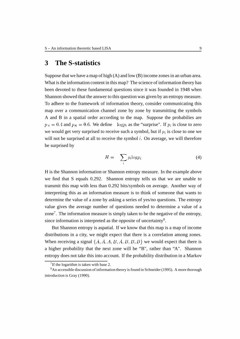
H is the Shannon information or Shannon entropy measure. In the example above

we find that S equals 0.292. Shannon entropy tells us that we are unable to

transmit this map with less than 0.292 bits/symbols on average. Another way of

interpreting this as an information measure is to think of someone that wants to

determine the value of a zone by asking a series of yes/no questions. The entropy

value gives the average number of questions needed to determine a value of a

zone7. The information measure is simply taken to be the negative of the entropy,

since information is interpreted as the opposite of uncertainty8.

But Shannon entropy is aspatial. If we know that this map is a map of income

distributions in a city, we might expect that there is a correlation among zones.

When receiving a signal fA;A;A;B;A;B;B;Bg we would expect that there is

a higher probability that the next zone will be “B", rather than “A". Shannon

entropy does not take this into account. If the probability distribution in a Markov

7If the logarithm is taken with base 2.8An accessible discussion of information theory is found in Schneider (1995). A more thorough

introduction is Gray (1990).


process with given p(B j B); p(B j A) etc. we are able to construct a code that in

fact transmits this map with less than 0.292 bits/symbol.

The terminology from communication theory of signals and bits should not

obscure the generality of the concept of information. The question of what is

the information content in a map is of more general interest, of course. Another

interpretation is the following. If we are to determine the value of a zone, we

are able to ask fewer questions, on average, if we know that there is a spatial

correlation among zones. Since we are using the information entailed in the

spatial configuration, we want to find a measure that takes space into account. In

this case, we expect the measure to be less than 0.292, and but not as small as zero

which would be the result if the symbol B was always followed by a B. On the

other hand, if there is no information in the spatial configuration, we would not be

able to use the spatial information to make the transmission more efficient.

In this paper we will use the spatial weighted information measure as hinted

above to derive a measure of spatial association. Like all similar measures of

spatial association, it is constructed by moving a spatial filter (a window) over the

spatial data (the map) and observing how the information is changed as we apply

the window at each location. If the information does not change very much, there

is a high degree of spatial association around that point. The measure derived in

this paper takes an information theoretic approach when explicitly defining the

concept of information.

3.1 Definition of the S statistics

Suppose we have a map with given probabilities to each zone. This is our original

information. If we wanted to see how much spatial information there is on the

map, we should first find out how much each zone is similar to its neighbouring

zones. In order to do that, we move a spatial filter over the map and observe how

the information changes as the window moves. After moving the filter over the

whole map, we get at the end a new map, possibly not so sharp as the original one,

a "blurred image". This new map is composed of new probabilities, which are

product of the geographical averages of original values taking into consideration


the values of the neighbouring zones. Its sharpness will depend on how much the

values of the original map are similar to the values of the their neighbours.

We could wonder how much information was lost by blurring the map, that

is, by losing information of the original spatial arrangement. Taking as a basis

the concepts of the Information theory we know that the average of uncertainty

or surprise is given by the negative of the sum of original probability times the

probability from the blurred map. Thus, if we have the average uncertainty we can

also find out the information we are looking for, S, since we assume Information

as the negative of average surprise.

S(p) = �(�X

i

pi log pi) (5)

where pi =P

j wijpj , and wij are the elements of a row-standardized spatial

weight matrix. If we have a prior distribution q, we include this to get

S(p; q;W ) = Eplogpi =X

i

pilogX

j

wij

pj

qj(6)

There is an intuitive interpretation of this measure. Suppose that we have two

types of individuals in an urban population, type A and type B and we pick an

individual of type A randomly. With probability pi we pick an individual in zone i.

Now we pick an individual of any type (A or B) in a neighbourhood of i according

to the probabilities wij . That is, with probability wij we pick an individual in cell

j. Given that the individual is from cell j, the probability that this individual will

also be of type A is pj=qj. The probability that we will pick an individual of type

A is hence equal toP

j wij pj=qj. The overall probability of picking an individual

of type A follows by taking the expected values over all zones. As argued earlier,

H is a measure of uncertainty. The more mixed the populations are, the more

uncertain we are whether we will pick an individual of type A or type B (high

entropy). The more segregated they are, the lower the uncertainty is (low entropy).

Thus, there is a nice intuitive interpretation of this measure, which is in fact

a spatial weighted Kullback-Leibler divergence measure9 (Kullback, 1959). The

9A probabilistic derivation of the Kullback-Leibler divergence measures is developed in


Kullback-Leibler divergence measures the distance between two distributions p

and q. From an information theoretic perspective, the measure S(p; q;W ) mea-

sures the information in p, given a priori information q and spatial configuration

entailed by the spatial weight matrix W . The information that is provided by the

spatial configuration can be measured by the difference

�(p; q;W ) = S(p; q; I)� S(p; q;W ) (7)

where I is the identity matrix, i.e. we do not take the spatial configuration into

account. S(p; q; I) is the Shannon information measure. For simplicity, let us

now surpress the q distribution and assume an uninformative uniform a priori

distribution. Then S(p; I) is a measure of the information of the data in the

map. Suppose now that we blur the data by applying a spatial averaging filter

to the data set. Then some information will be lost. The amount of information

that is lost by the spatial filter is the difference S(p; q; I) � S(p; q;W ). If the

neighbourhoods of each location are very similar to the location itself, blurring the

data loses little information, and the difference becomes small. On the other hand,

if data are spatially heterogeneous, then blurring the data loses a lot of information

and the difference becomes large. If the difference is small, then we have much

information if we just have the spatial average data. In such a case, there is a high

degree of spatial association. If the difference is large, there is little information

in the spatial configuration itself, and there is less spatial association.

In the application below we will use the conditional permutation approach to

establish significance bounds on the local statistics. By randomly permuting the

data, we can establish an empirical distribution of the S statistics. Let us denote

the expected value of S under the randomisation hypothesis by Sr. Then we may

define the index

� =S � Sr

S0 � Sr(8)

Note that � <= 1, with equality if the neighbourhood of each location is identical

to the location itself, i.e. maximum spatial association. If each neighbourhood

Snickars and Weibull (1977).


is just a random subset of all observations, we have � = 0. If we have spatial

segregation (or negative spatial association), we have � < 0.

The global S statistics is similar to the Moran’s I in the sense that a positive

index � indicates positive spatial association, i.e. similar values are clustered with

similar values. A negative � indicates negative spatial association, i.e. dissimilar

values are clustered with each other.

The difference S � Sr is a measure of the information contained in the spatial

averaged data, compared to a random permutation of the data set. Information

should be interpreted as a decrease of uncertainty. Suppose that we do not have

the final data set, but we are given a spatial averaged data. � is a measure of

how much the uncertainty is decreased as we move from a completely random

permutation of the data set, to spatial filtered data. If there is a high degree of

spatial association, with similar values clustered, we will decrease the uncertainty

of the final data considerably, and � is close to one. On the other hand, if there is

no positive spatial association, the uncertainty will not be decreased and � is close

to zero.

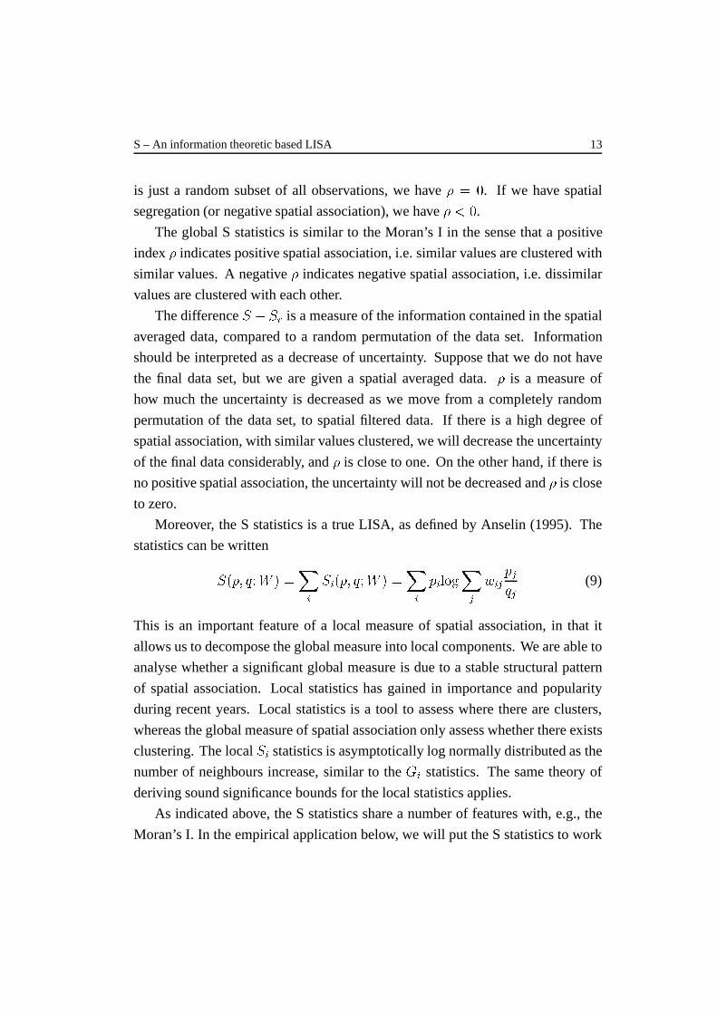
Moreover, the S statistics is a true LISA, as defined by Anselin (1995). The

statistics can be written

S(p; q;W ) =X

i

Si(p; q;W ) =X

i

pilogX

j

wij

pj

qj(9)

This is an important feature of a local measure of spatial association, in that it

allows us to decompose the global measure into local components. We are able to

analyse whether a significant global measure is due to a stable structural pattern

of spatial association. Local statistics has gained in importance and popularity

during recent years. Local statistics is a tool to assess where there are clusters,

whereas the global measure of spatial association only assess whether there exists

clustering. The local Si statistics is asymptotically log normally distributed as the

number of neighbours increase, similar to the Gi statistics. The same theory of

deriving sound significance bounds for the local statistics applies.

As indicated above, the S statistics share a number of features with, e.g., the

Moran’s I. In the empirical application below, we will put the S statistics to work


and compare the global S and I, as well as the local Si and Ii. It will be shown

that the S and I statistics are different in that the local statistics differ for zones

with small values. Zones with small values are not picked up as contributing

to the global association. In this sense, the S statistics behaves more like the

Gi statistics, indicating zones with high degree of spatial association where high

values are associated with high values. However, the S statistics can be summed to

give a global measure of spatial association, as opposed to the Gi statistics which

is not a true LISA.

The local statistics Si can be given different interpretations along the lines

put forward above. Seen as a segregation measure, the local Si statistics give

the probability that we will pick an individual of type A (following the spatial

distribution p) in zone i, and that the next individual in a neighbourhood of i also

will be of the same type. Note that if there are very few individuals of type A in

zone i, the local measure Si will be low.

In an information theoretic interpretation�measures the degree of information

that is entailed in the spatial configuration itself. If there the spatial configuration

was only arbitrary, and there is no spatial association, then much information

would be lost by taking a geographical average. If there is a high degree of spatial

association, much less information is lost by taking a geographical average, and

S is close to S0 Expressed in another way, we do have much information if we

are given the spatial averaged data. The difference can be decomposed, such that

the information lost by blurring around each location can be examined. If there

is a high degree of spatial association around a location, and the neighbourhood

look very similar to the location itself, this location would not contribute much to

the information loss by blurring (taking the geographical average). That is, we

have almost all information already in the geographically averaged data around

that location.

Si is similar to Gi in that zones with high values with positive association will

give a high value of the local statistic. Local Moran’s I, on the other hand, may

have a high value even if the attribute values are close to zero. Such differences

between the different measures are important to understand, since it shows that


the measures S, G and I do different things. As will be shown in the application,

the local Si and Gi are very similar, but Si can be aggregated to give a measure of

global association.

To summarise, we have defined an S statistics that is a measure of global and

local spatial association. This measure has a few advantages:

(i) S has simple intuitive interpretation in the context of spatial segregation

(ii) S can be decomposed into local measures of spatial association, indicating

each location’s contribution to the global measure

(iii) S has a natural extension to bivariate distributions. The bivariate measure

gives an interpretation of the commonly used empirical Bayesian method as a

Kullback-Leibler divergence measure

(iv) The measure scales the local contributions according to their values, such

that locations with positive association and high values contribute more to the

global measure than locations with small values. In this respect, S behaves more

like the Gi statistics, but it has the advantage of being possible to aggregate to give

a global measure of spatial association (it is a true LISA).

(v) S is asymptotically normal distributed. Si is asymptotically log-normal

distributed as the number of neighbours grows.

4 Methodological procedures and results

4.1 The case-study area

Stockholm is the capital of Sweden and its biggest city. Almost half of Greater

Stockholm’s inhabitants live in Stockholm. The city of Stockholm had over 720

000 inhabitants in 1998, while the Greater Stockholm area had over 1,6 million

inhabitants. The case-study area is composed of Greater Stockholm, that is, the

city of Stockholm as well as its 24 municipalities.

Stockholm City has, compared to other Swedish cities, a high population den-

sity of 1300 inhabitants/km2, while Stockholm County has 266 inhabitants/km2.

Only a few areas of the inner city are densely populated. During 1950 to 1985,


the inner city area lost nearly 200 000 inhabitants. The decrease in population

within the city of Stockholm is partly explained by the conversion of building

space into offices. However, the demand for apartments within Stockholm City

has during the last few years created a need for building companies to make avail-

able as many apartments as possible by renewing old areas, especially industrial

ones. The real estate market has changed and signals of a gentrification process

are already evident in certain areas of the inner city.

The Stockholm CBD is located in the southern area of the inner city and is

characterised by many office buildings and a number of large department stores.

Not only the governmental and ministerial buildings are located in this area but

also the major shopping area of the city, as well as theatres, museums, restaurants,

bars and cinemas. The main public transport junction is located in the CBD area.

All underground lines pass through the Central Station, which is the main railway

station of the capital, making this area a place where many travellers pass everyday.

The real estate market is characterised by having high valued housing in

the inner city and surroundings. In Stockholm City, about 90 per cent of the

dwellings are composed of multi-family houses, the rest are single-family houses.

Rented accommodation is common both in Greater Stockholm and the city itself.

Two out three dwellings are rented; almost all the rest is tenant owned housing.

In Stockholm, as in other large European cities, geographic, ethnic and socio-

economic segregation has increased during the last decade as a result of, amongst

other things, a decrease in income and income mobility (SOU 1998:25, Sandstrom,

1997).

4.2 Culture sector in Stockholm County

Culture in Stockholm County, as in other parts of Sweden, has traditionally re-

ceived a large financial support from the State. The Swedish model with arts

and culture as a publicly financed good has always been a part of the established

welfare state. However, structural socio and economic changes during the nineties

has opened up culture for other partners beyond the public sector, creating new

areas of activity within the culture industries never thought of before and also new


ways to stimulate culture through co-operation between public and private actors.

For a more extensive discussion of these issues, see Gnad (1999).

In Stockholm County, the selected culture sectors employ approximately 6 per

cent of the total employed population. An increasing number of workplaces have

been verified in these seven branches since the beginning of the 1990’s, mostly in

“artistic and literary activities, film and video production and theatres and concert

houses". Besides, significant changes in enterprise size (number of employees)

have also occurred during the same period of time. Data from 1993 to 1998 shows

that the most significant changes are concentrated to three branches: artistic and

literature activities, theatres and concert houses, museums and culture heritage.

All these branches have had a marked decreasing in the number of employees.

New forms of contracts (subcontract) may explain the decrease of number of

employees in, at least, the last two named branches.

The question that remains is: What does the spatial pattern of employment of

the culture sector look like in Stockholm County?

Regarding their spatial distribution, it can be expected that these seven sectors

basically follow two types of patterns: a group of more stable culture activities

in terms of localisation over time, such as museums and culture heritage and,

to a certain extent, theatres and concert houses, film and video presentation.

This group is part of a more institutionalised type of culture, mostly publicly

financed and characterised by having several employees or subcontractors. Since

Stockholm County is still very polarised by the Stockholm’s inner city, where the

CBD and other related activities are concentrated, one could expected that clusters

of these more stable culture activities would also be concentrated there. Using

principles of locational advantages, one could say that these activities would be

better off if they would be located in the proximity to enterprises in the cultural

sector (attraction points of urban visitors), proximity to related-cultural enterprises

(hotels, restaurants, shops, other entertainment) and have a good infrastructure

regarding accessibility to other places.

The second group is composed of activities that are more vulnerable to the

fluctuations of the regional economy, their spatial location is more flexible and


they might change their location over time or even disappear. They are mostly

constituted by small enterprises, often the artist her/himself (en-mansforetag).

Examples of this kind are found in the branch Artistic and Literary Activities, film

and video production and film and video distribuition. The initial hypothesis is that

clusters for these cultural activities will appear outside of the core of Stockholm’s

City for the following reasons: (1) these cultural activities are not dependent on

proximity to consumers or other related-cultural enterprises (2) pressures from the

real estate market make it difficult or even impossible for more vulnerable culture

activities to start up and remain as enterprises in the Stockholm inner city, and (3)

the branch of park of entertainment (amusement parks) requires a large amount of

land that are often available outside of the region main centre.

4.3 The culture sector data set

The statistical data set of the culture sector (total number of work places by co-

ordinate) used in this study of Stockholm County has been extracted from the

database of Statistics Sweden. Seven branches were selected constituting 5065

work places composing about 51 600 jobs in 1998. Data on total employment

for each branch was later attached to the basic unit of analysis - the 1248 wards

over Stockholm County. The total number of employed by each of the seven

culture branches was then associated to each ward as well as the total number

of daily working population (dagbefolkningen), the closest indicator for the total

employment in each ward. For the statistical analysis the proportion of employees

in the selected seven sectors by each ward was estimated.

In order to have a robust data set a few adjustments were carried out. Regarding

the data of total employment by ward, it is worth noting that empty wards, such

as areas with no population and work places, were eliminated from the analysis.

Thus, approximately 7 per cent of the statistics of total employment could not be

mapped since there was no spatial information attached to the wards. Regarding

the culture data by branch almost 2% of the wards had inconsistent data. In these

cases the total number of employees in a certain culture branch and area was

greater than the total number of employees in each branch. Most of the cases,


these areas had an overrepresentation of number of employees of specific branch.

In order to minimise this source of error, we decided to assume the total number of

unemployed people in each ward as a basis for calculation. Thus, the total number

of employees for each ward was distributed to each branch proportionally using

as basis the original distribution for each branch and ward.

4.4 Measuring global and local spatial association in the culture

sector

SpaceStat (see Anselin, 1992) was used to calculate the global and local Moran’s

I. The chosen method of inference about the significance of I was permutation (99

random permutations) and the used weight matrix was row standardised (a simple

0/1 matrix where 1 indicates that the zones have a common border). The results

of the global Moran’s I are presented in Table 2.

Gi-statistics were also calculated using SpaceStat. An adjacency weight matrix

was used to calculate Gi*. A positive and significant z-value indicates spatial

clustering of high values, whereas a negative z-value indicates spatial clustering of

low values. A Bonferroni bound procedure was used to assess significance in order

to take account of the effect of multiple testing. So, using an overall significance

level of 0.01, the significance level for each individual test score is set to 0.01/1248,

or 0.000008. Since the Bonferroni bound procedure is likely to be conservative

(increased risk of a type II error), we assumed the original significance level of

0.01. Finally, maps were created using a Desktop Mapping System (MapInfo)

showing areas with concentrations of offences, which are statistically significant

(p =< 0.05) for the study area. The resulting clusters are discussed in section 4.6.

The S statistics was calculated with the OX package, Doornik (1998). Ox

is a statistics and mathematics package, similar to GAUSS and MATLAB. It

is fast (at least in the same magnitude as GAUSS), and it allows for object-

oriented programming. The spatial weight matrix was constructed with utilities

of SpaceStat package.


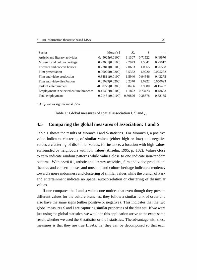
Sector Moran’s I S0 S �a

Artistic and literary activities 0.45025(0.0100) 1.1307 0.71522 0.49970

Museum and culture heritage 0.22681(0.0100) 2.7973 1.5841 0.25017

Theatres and concert houses 0.23811(0.0100) 2.0663 1.0365 0.26558

Film presentation 0.06025(0.0200) 3.5352 1.9220 0.075252

Film and video production 0.34811(0.0100) 1.5940 0.94546 0.43275

Film and video distribution 0.05029(0.0200) 3.2370 1.6222 0.050693

Park of entertainment -0.00775(0.0300) 5.0406 2.9380 -0.15487

Employment in selected culture branches 0.45497(0.0100) 1.1822 0.73473 0.48603

Total employment 0.21481(0.0100) 0.80896 0.38878 0.32155

a All � values significant at 95%.

Table 1: Global measures of spatial association I, S and �.

4.5 Comparing the global measures of association: I and S

Table 1 shows the results of Moran’s I and S-statistics. For Moran’s I, a positive

value indicates clustering of similar values (either high or low) and negative

values a clustering of dissimilar values, for instance, a location with high values

surrounded by neighbours with low values (Anselin, 1995, p. 102). Values close

to zero indicate random patterns while values close to one indicate non-random

patterns. With p<=0.01, artistic and literary activities, film and video production,

theatres and concert houses and museum and culture heritage indicate a tendency

toward a non-randomness and clustering of similar values while the branch of Park

and entertainment indicate no spatial autocorrelation or clustering of dissimilar

values.

If one compares the I and � values one notices that even though they present

different values for the culture branches, they follow a similar rank of order and

also have the same signs (either positive or negative). This indicates that the two

global measures S and I are capturing similar properties of the data set. If we were

just using the global statistics, we would in this application arrive at the exact same

result whether we used the S statistics or the I statistics. The advantage with these

measures is that they are true LISAs, i.e. they can be decomposed so that each


location’s contribution to the global measure can be examined. In the next section

we will show that the local Sistatistics behaves similar to the local Iistatistics, but

that there are important differences. Although the global statistics are similar, the

measures capture different aspects of the spatial pattern of association. In fact,

when examining the spatial pattern of local Si, Ii, andGistatistics, it will be shown

that the SiandGiare more similar than the Siand Iistatistics. This will demonstrate

one important contribution of the Sistatistics.

4.6 Comparing the local measures of association: Ii , Gi* and

Si-statistics

Local measures of spatial association define how much each observation con-

tributes to the global measure of spatial association. In this study, three measures

of local spatial association have been carried out, namely Local Moran’s I , Giand

Si-statistics. The objective here was to see to what extent these measures differ

from each other and try to find out if S-statistics could contribute to better under-

stand the global pattern of spatial association and if it did, to identify which was

the main contribution to the proposed measure.

As was pointed out in section 4.5, the global measures of spatial association I

and � were quite similar for the selected culture branches. Thus, the question that

remains to be answered is: to what extent does a single observation contribute to

the global measure of spatial association?

The distribution of local statistics of Si, Giand Iiis depicted in Figure 1. The

distribution of Siand Iilooks similar. The distribution of locations yielding the

highest contribution to the global I and S measures are thus similar. To examine

each locations contribution to the global measures, Figure 2 show the Iistatistics

plotted against the Sistatistics. Figure 2 (a) illustrates how Iiand Siare correlated.

However, looking at the results more carefully, one realises that Iiand Sibehave

differently for attribute values close to zero, that is, polygons with small pi:s. While

Iishows indications of autocorrelation for small attribute values,Sieliminates these

small values resulting in a more robust measure of local association (Figure 2b).


Figure 1: Distribution of local Ii, Si, and Gistatistics.


Figure 2: a) Ii and Sifor variable Film production (b) Detailed picture of values

around zero of Sivs. Ii.

Figure 3: a) Gi* and Sifor variable Film production (b) Detailed picture of values

around zero of Sivs. Gi*


A similar pattern can be found when comparing Gi* and Siresults. They are

correlated and again Gi* appears to be more sensitive to attribute values close to

zero, while Sicuts down values that does not contribute very much to the global

measure (Figures 3(a) and (b)).

The Sistatistics behaves differently for small values than both the Iistatistics

and Gistatistics. However, when studying the significant clustering under the

randomization hypothesis, theSistatistics behaves much more like theGistatistics.

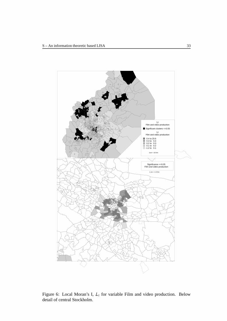
Figures 4,5 and 6 illustrate on maps the three local measures of spatial association

for variable Film production over the whole Stockholm County and in detail,

showing only those clusters that are significant at 0.05 level. As it could be

expected, the spatial distribution of Gi* values is very similar to Si. The highest

values of Gi* and Sifor film and video production, for instance, are concentrated

in Stockholm City and surrounding areas while the significant clusters are limited

only to the inner city areas, but not in a homogenous way, the pattern excludes

the northern parts of the city residential core. It is worth noting that the spatial

pattern of significant values of local Moran’s I is more spread than those of

Gi* and Si, showing also high values of autocorrelation in the outer areas of the

Stockholm County. In these peripheral areas, the branch film and video production

is virtually non-existent, thus, a group of zero-attribute polygons had appeared to

have significant values of I, and possibly inflating the global I measure.

A common feature of these measures is that they provide information on how

each region’s attribute on space contribute to the global measure and once mapped

they can also help to identify pockets of spatial association as well as indicate the

characteristics of stability in the data set (Appendix 1 illustrate the characteristics

of the data set regarding the distribution of the local spatial measures over the whole

study area). However, each measure may give its highest degree of contribution

dependent upon the questions to be answered and on area of application. S statistic,

as local measure of spatial association, gives its highest contribution to areas of

analysis that look for an indicator that works asGibut at the same time still function

as a LISA - Local Indicator of Spatial Association.


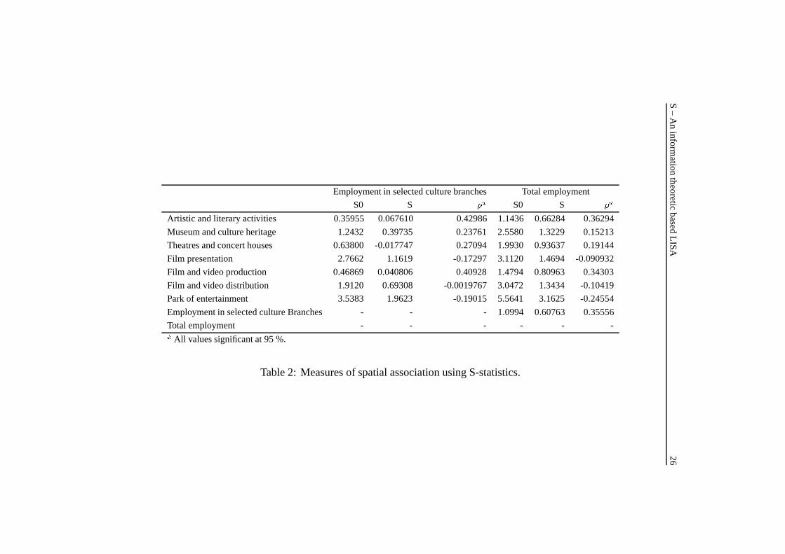
4.7 Measuring spatial association using S-statistic by a priori

distribution variable q

Table 2 summarises the results of S when p is standardised by a priori distribution

variable. In this case, p was employment by each culture sector divided by q, that

was either total employment in the selected culture branches or total employment

in each region (polygon). S is, in this case, an indicator of how similar the spatial

distribution of each culture branch is in relation to the a priori distribution variable.

Note that the pure Shannon information measure, S0, decrease at the same time

as the number of observations decrease. Few culture branches such as, film and

video presentation, park of entertainment and film and video distribution had a

negative �, which might indicate that this measure is sensible to small number of

observations. A partial solution to this limitation would be to create larger and

more robust geographical units that constitute a satisfactory basis for statistical

analysis, as suggested by Wise et al. (1997); Haining et al. (1998).

As expected, the S statistics with an uninformative uniform prior for each

culture sector is higher than the corresponding statistics with an informative prior

distribution q.

4.8 Analysing the spatial pattern of employment in the culture

branches: Implications of S-measures

A special feature of S statistic is that it provides a measure of concentration

of employment within each culture branch taking into consideration its spatial

distribution. What does the spatial pattern of employment of the culture sector

look like in Stockholm County?

Two distinct patterns of spatial pattern of employment in the culture sector were

expected. The first pattern would be determined by more "stable" culture activities

in terms of localisation over time, such as theatres and concert houses, museums

and to a certain extent culture heritage, film and video presentation (cinemas)

would be concentrated in the inner city of Stockholm. It was expected that the

second pattern would have a more suburbanised character, constituted mostly

S–

An

information

theoreticbased

LISA

26

Employment in selected culture branches Total employment

S0 S �a S0 S �a

Artistic and literary activities 0.35955 0.067610 0.42986 1.1436 0.66284 0.36294

Museum and culture heritage 1.2432 0.39735 0.23761 2.5580 1.3229 0.15213

Theatres and concert houses 0.63800 -0.017747 0.27094 1.9930 0.93637 0.19144

Film presentation 2.7662 1.1619 -0.17297 3.1120 1.4694 -0.090932

Film and video production 0.46869 0.040806 0.40928 1.4794 0.80963 0.34303

Film and video distribution 1.9120 0.69308 -0.0019767 3.0472 1.3434 -0.10419

Park of entertainment 3.5383 1.9623 -0.19015 5.5641 3.1625 -0.24554

Employment in selected culture Branches - - - 1.0994 0.60763 0.35556

Total employment - - - - - -

a All values significant at 95 %.

Table 2: Measures of spatial association using S-statistics.


of clusters of small enterprises, having a more spread spatial pattern, composed

of a series of small clusters around the whole County. This pattern would be

particularly true for the following branches: artistic and literary activities, park of

entertainment and film and video production and film and video production.

Findings from Si (calculated using a priori distribution variable q, in this case,

total employment) suggest that the expected spatial pattern is pretty much in line

with the hypothesis proposed to the first group of branches. A brief analysis

of maps of the significant clusters for these four branches show a strong spatial

concentration in Stockholm’s inner city, where the CBD and other related activities

are located. However, different sectors determine the pattern and the exact location

of these clusters. Employment in the museum and culture heritage’s branch shows

a concentration of in the centre-Northeast areas of the city core. Contrary to what

was expected, clusters of employment in the branch of film and video production

were also located in parts of the inner city, with a very similar spatial pattern to

the branch film and video distribution, composed mostly of four or five set of

zones. Employment in cinema or the so-called film presentation show several

small clusters in the inner city but also two significant clusters located outside

of Stockholm city, mostly concentrated in large suburban areas. Following a

similar pattern, employment in the branch of theatres and concert houses is heavily

concentrated in southern and northwest but also exhibit several clusters in other

municipalities of the Stockholm County.

As was expected, employment in the branch of park of entertainment (amuse-

ment parks) exhibits a more spread pattern even outside of Stockholm City. Sur-

prisingly, no significant cluster for the branch artistic and literary activities was

found outside Stockholm inner city. Even though it was already known that this

branch was composed mostly of small enterprises (thus, low concentration of

jobs), at least few clusters spread all over the county were expected. These find-

ings corroborate to the argument that S-statistic mostly pick up the most robust

clusters of the distribution, eliminating the smaller ones, in this case, those located

in the outer city.

The map showing the significant clusters S-statistics for employment in the


seven selected culture branches together illustrates the concentrated spatial pattern

to the inner areas of Stockholm City.

5 Final considerations

We have addressed the question of what information is contained by the spatial

configuration of spatial data. We developed a spatial weighted information mea-

sure that enable us to determine the amount of information that is lost if the spatial

configuration is lost. By moving a spatial filter over the data set, we may use

this information measure to assess the information content of space around each

location, giving rise to a local statistics of spatial association. If the neighbourhood

of a location is very similar to the location itself, there is not much information

lost by blurring the data with a spatial filter, indicating a high degree of spatial

association. Furthermore, the sum of the local statistics is an information mea-

sure. Hence, we also have introduced a global measure of spatial association. By

decomposing the global measure into the local counterparts, we have been able to

assess the structure stability of the global measure.

The proposed S statistics was applied to a data set of employment in the cultural

sector of the Stockholm area. The global S statistics was shown to give the same

results as the global Moran’s I statistic, both in the case of positive and negative

autocorrelation. The local statistics of Si, Iiand Giare quite correlated, but a

distinct feature of the Sistatistics is the treatment of locations with values close

to zero. The significant local statistics of Siand Giwere very similar, in contrast

with significant Iistatistics. If we study the significant local statistics with Sior

Gi, similar results emerge. However, the Sistatistics can be aggregated to a global

statistics to assess global spatial association, in contrast with the Gistatistics that

not is a true LISA.

Furthermore, theSistatistics has a natural extension to bivariate variables,using

the Kullback-Leibler divergence measure. This formulation gives a statistical and

information theoretic interpretation to the commonly used empirical Bayesian

approach.


For future studies, more attention should be paid to the relationships between S,

I and Gi as well as to the process of building more robust geographical units that cer-

tainly contribute to a more satisfactory basis for statistical analysis.Measurements

of negative spatial association of S statistic should also be further exploited. The

use of unrelated variables when running S-statistic by a priori distribution should

also be taken into consideration in order to have more reliable results. Time di-

mension is also an important aspect when studying spatial patterns and therefore

could be incorporated into S statistics, increasing its analytical capacity.

ReferencesAnselin, L. 1992. SpaceStat tutatorial - a workbook for using SpaceState in the analysis of

Spatial Data. Regional Research Institute, West Virginia University, Morgantown.Anselin, L. 1995. Local indicators of spatial association - LISA. Geographical analysis.

2:94-115.Batty, M., 1974, Spatial entropy, Geographical Analysis, 6, pp. 1–31.Batty, M. , 1976, Entropy in spatial aggregation, Geographical Analysis, 8, pp. 1–21.Bivand, R. 1998, A review of spatial statistical techniques for location studies.CEPR

symposium on new issuesin trade and location, Lund, 1-21.Boots, B.N. and Getis, A. 1988, Point pattern analysis.Scientiphic Geography series.8,

SAGE publications.Cliff, A.D. and Ord, J.K. 1973, Spatial autocorrelation, (London: Pion).Christakos, G. 1990, A Bayesian/Maximum-Entropy View to the Spatial Estimation

Problem, Mathematical Geology, 22(7), 763-777.Clark. P.J., and Evans, F.C., 1954, Distance to nearest neighbour as a measure of spatial

relationshhips in populations, Ecology, 35, pp. 445–453.Denbigh, K.G. and Denbigh, J.S., 1985, Entropy in relation to incomplete knowledge,

Cambridge University Press.Doornik, J.A. 1998, Object-Oriented Matrix Programming using Ox 2.0, London: Tim-

berlake Consultants Ltd and Oxford.Getis, A. and Ord, J.K. 1992, The analysis of spatial association by use of distance

statistics. Geographical analysis. 4:189-206.Goodchild, M.F. 1986, Spatial autocorrelation - concepts and techniques in modern

Geography, ISSN 0306-6142; 47.Gnad, F. 1999, The contribution of culture industries to urban and regional development.

In: City and culture, (Workshop 7: Culture, Economic change and sustainabledevelopment), Stockholm Sweden, 1-15.

Gray, Robert M., 1990, Entropy and Information Theory, New York: Springer Verlag.


Haining, R Wise, Ma, J. 1998, Exploratory spatial data analysis in a geographic infor-mation system environment, The Statistician, 47:457-469.

Jaynes, E.T., 1957, Information theory and statistical mechanics. Physical Review,106(4):620-630, 1957.

Journel, AndrZ G., and Deutsch, Clayton V., 1993, Entropy and Spatial Disorder, Math-ematical Geology, 25, pp. 329–?.

Kullback, S., 1959, Information and statistics, New York: Wiley.Lee, Y.-M, 1998, A methodological study of the application of the maximum entropy

estimator to spatial interpolation, Journal of Geographic Information and DecisionAnalysis, 2(2), pp. 265-276.

Lee, Yuh-Ming and J. Hugh Ellis, 1997, On the Equivalence of Kriging and MaximumEntropy Estimators, Journal of Mathematical Geology, Vol.29, No.1, pp.131-152.

Legendre, P., and Legendre, L., 1998, Numerical Ecology, Second edition, Amsterdam:Elsevier.

Leung, C.K., and Lam, F.K., 1996, Maximum segmented-scene spatial entropy thresh-olding, IEEE something, pp. 963–966.

Pielou, E.C., 1961, Segregation and symmetry in two-species populations as studied bynearest neighbour relationships, Journal of Ecology, 49, 255–269

Pielou, E.C., 1969, An Introduction to Mathematical Ecology, Wiley & Sons.Sandstrom, C. 1997. Bostadsformedling och segregation, USK-aktuellt, 2:35-39.Schneider, Tomas D., 1995, Information Theory: a Primer, working paper.Skilling, J, 1991, Fundamentals of MaxEnt in data analysis, in Buck, Brian, and

Macaulay, Vincent A. (eds) Maximum entropy in action: Oxford Science Pub-lications, pp. 19–40.

Snickars, F., and Weibull, J.W., 1977,A minimum information principle: Theory andpractice, Regional Science and Urban Economics, 7, pp. 137–168.

Socialdepartementet, 1998, Tre stader: en storstadspolitik for hela landet, Stockholm:SOU:1998:25.

Wise, S.M Haining, R.P, Ma, J, 1997, Regionalisation tools for the exploratory spatialanalysis of the health data. In: Recent Developments in Spatial Analysis: SpatialStatistics, Behavioural Modelling and Neuro-computing, M. Fisher and A. Getis(eds), 83-100. Berlim:Springer.

Appendix


SiFilm and video production

Significant clusters <=0.05

SiFilm and video production

0.0004 to 0.07630.0003 to 0.00040.0002 to 0.00030.0001 to 0.0002

-0.002 to 0.0001

1cm = 10 Km

1 cm = 1.5 Km

Significance <=0.05Film and video production

Figure 4: Si for variable Film and video production. Below detail of centralStockholm.


Gi*Film and video production


Gi*Film and video production

-0.1 to 10.9-0.3 to -0.1-0.6 to -0.3-0.8 to -0.6-1.5 to -0.8

1cm = 10 Km

1 cm = 1.5 Km

Significant clusters <=0.05Film and video production

Figure 5: G�

i for variable Film and video production. Below detail of centralStockholm.


LiFilm and video production


LiFilm and video production

0.4 to 20.60.3 to 0.40.2 to 0.30.1 to 0.2

-1.2 to 0.1

1cm = 10 Km

1 cm = 1.5 Km

Significance <=0.05Film and video production

Figure 6: Local Moran’s I, Li for variable Film and video production. Belowdetail of central Stockholm.

A new information theoretical measure of global and local spatial association

Documents

Transcript of A new information theoretical measure of global and local spatial association