A New Fuzzy Connectivity Measure for Fuzzy Sets

J Math Imaging Vis (2009) 34: 107–136DOI 10.1007/s10851-009-0136-3

A New Fuzzy Connectivity Measure for Fuzzy Sets

And Associated Fuzzy Attribute Openings

Olivier Nempont · Jamal Atif · Elsa Angelini ·Isabelle Bloch

Published online: 14 February 2009© Springer Science+Business Media, LLC 2009

Abstract Fuzzy set theory constitutes a powerful represen-tation framework that can lead to more robustness in prob-lems such as image segmentation and recognition. This ro-bustness results to some extent from the partial recovery ofthe continuity that is lost during digitization. In this paperwe deal with connectivity measures on fuzzy sets. We showthat usual fuzzy connectivity definitions have some draw-backs, and we propose a new definition that exhibits betterproperties, in particular in terms of continuity. This defin-ition leads to a nested family of hyperconnections associ-ated with a tolerance parameter. We show that correspond-ing connected components can be efficiently extracted usingsimple operations on a max-tree representation. Then we de-fine attribute openings based on crisp or fuzzy criteria. Weillustrate a potential use of these filters in a brain segmenta-tion and recognition process.

This work has been partly supported by a grant from the NationalCancer Institute (INCA).

O. Nempont (�) · E. Angelini · I. BlochTELECOM ParisTech, CNRS LTCI, UMR 5141, 46 rue Barrault,75013 Paris, Francee-mail: [email protected]

E. Angelinie-mail: [email protected]

I. Bloche-mail: [email protected]

J. AtifUS ESPACE, IRD-Cayenne, route de Montabo, BP 165,97323 Cayenne, French Guianae-mail: [email protected]

Keywords Connectivity · Fuzzy sets · Connected filters ·Mathematical morphology · Hyperconnection · Max-tree ·Fuzzy attribute opening

1 Introduction

Connectivity is a key concept in image segmentation, filter-ing and pattern recognition, where objects of interest are of-ten constrained to be connected according to some definitionof connectivity. This definition depends on the selected ob-ject representation. Binary representation on a discrete gridremains the most widespread, and the connectivity is thengenerally derived from an elementary connectivity, such as4- or 8-connectivity in 2D (for a square grid).

In [38], Serra introduced the notion of connection as anaxiomatization of the classical definitions of connectivity.A connection (also referred to as connectivity class) on aspace E is a family of subsets of E that are said connected.Among others the connected subsets of a binary image, thearc-connected subsets of R

n or the connected subsets of agraph can be represented by a connection. Another equiva-lent axiomatization was proposed by Ronse in [29]. Basedon connections derived from usual notions of connectivity,more complex connections can be obtained. For instancewe can assume that a subset is connected if its dilationis [14, 29], consider connections in attribute spaces [48] ormake use of nested connections to represent multiscale con-nectivity [5].

Connections are closely related to connected operators(i.e. operators that manipulate only connected componentsaccording to a definition of connectivity). For example, con-sidering a usual connection on the digital space, connectedfilters for binary images [12, 18, 37] modify only connected

mailto:[email protected]




108 J Math Imaging Vis (2009) 34: 107–136

components of the object or of the background, without cre-ating new boundaries nor moving existing ones.

In [40] the framework of connections was extended togeneral complete lattices and to the notion of hypercon-nectivity (i.e. based on a more general definition of over-lap), in particular to represent connectivity on grey scale im-ages [7, 41]. Further properties of connections on completelattices were given in [4, 31]. Connected filters for grey-levelimages [36, 46] were proposed independently, generally re-lying on the notion of flat-zones (i.e. the largest connectedregions with constant grey level). Those filters were recentlygeneralized to connective segmentation [30, 32, 42].

From a computational point of view, connected filteringis generally efficiently performed using a tree representa-tion of the image. The well known max-tree representation(also referred to as the component tree [16, 25] or openingtree [47]) was introduced in [35] to compute attribute open-ings [8] and can be built using efficient algorithms [1, 19, 23,25, 49]. The max-tree representation has also been extendedto handle second-generation connectivity [28]. The tree ofshapes proposed in [24] introduces a contrast-invariant treerepresentation of the image that allows the computation ofmore complex filters.

In this paper we deal with connectivity of fuzzy sets de-fined on the digital space and with associated connected at-tribute openings. Object representation using fuzzy sets [51]enables to model various types of imperfections, in partic-ular related to image imprecision. Considering fuzzy repre-sentations of objects (for instance in an image segmentationand recognition process) can lead to more robustness thatresults, to some extent, from the partial recovery of the con-tinuity that is lost during the digitization process. Howeverthe use of fuzzy representations leads also to more com-plexity in the definition of filters and their numerical im-plementation. Extending filters for binary sets to filters forfuzzy sets is sometimes possible, for instance using the ex-tension principle [50]. The result of that extension is gener-ally quite different from extensions to grey-level images. Forinstance when dealing with connected filters, the binary def-inition can be extended to the grey-level case stating that theconnected components of a grey-level image are the largestregions that present a constant grey-level. Such filters areknown as flat-zones connected filters [36, 46]. Obviouslythis extension does not make sense for fuzzy sets, since thesemantics of pixels values is quite different. The values of afuzzy set refer to a membership degree to a set while there isin general no obvious relation between grey-levels and theirvariations and membership degrees. Since in the binary casethe connected components of a set are sets, the connectedcomponents of a fuzzy set should in the same manner bedefined as fuzzy sets. Connectivity for fuzzy sets and con-nected operators thus need a specific definition that reallytakes into account the semantics of the membership values.

Table 1 Main notations

Notation Definition

X Spatial domain, i.e. a bounded subset of Zn

μ A fuzzy set on X, i.e. a mapping from X to [0,1](μ)α α-cut of μ

F Set of all fuzzy sets on X

H1 Set of connected fuzzy sets according to (1)

H1τ Set of connected fuzzy sets according to (2)

H2τ Set of connected fuzzy sets according to (4)

c1μ(x, y) Point to point connectivity degree with respect to

a fuzzy set μ (cf. Definition 1)

c1(μ) Connectivity degree of μ as defined by (3)

c2(μ) Connectivity degree of μ according to Definition 6

δtx(y) Impulse function: δt

x(y) = t if y = x and 0 otherwise

⊥1, ⊥1τ , ⊥2

τ Overlap mappings associated to H1, H1τ and H2

τ

In [33, 34], Rosenfeld proposed a first definition of fuzzyconnectivity between points in the digital space accordingto a fuzzy set. Based on this definition, he derived a charac-terization of the connectivity of a fuzzy set, known as topo-graphic connectivity. According to this characterization, afuzzy set is connected if it presents a unique regional maxi-mum or equivalently if all its α-cuts are connected. A similardefinition for fuzzy sets on continuous spaces was proposedin [20].

Its later extension [6] leads to a characterization of theconnectivity as a degree, defined as the membership degreeof the lowest saddle point. This degree is however not con-tinuous with respect to the membership function.

Therefore we propose a new definition that exhibits bet-ter properties, in particular in terms of continuity. We willshow that this definition can be appropriately represented bya hyperconnection.

We first recall in Sect. 2 some preliminary definitionson fuzzy sets, connections and fuzzy connectivity. We il-lustrate in particular some of their drawbacks. In Sect. 3,we introduce a new connectivity measure, and we show thatit leads to a nested family of hyperconnections indexed bya tolerance parameter, with nice continuity properties. Hy-perconnected components are then defined, and an extrac-tion scheme based on a max-tree representation is proposed.These notions lead to the definition of filters over hypercon-nected components and in particular to attribute openingsthat may be used in a combined segmentation and recogni-tion process. A generic formulation of such filters is given inSect. 4, and in Sect. 5 two practical examples are presented.The first one illustrates the use of a fuzzy marker, while thesecond one makes use of a fuzzy volume prior. Both filtersare illustrated in a recognition process on a brain magneticresonance image (MRI). Proofs of all propositions are pro-vided in Appendix. Table 1 brings together the main nota-tions.

J Math Imaging Vis (2009) 34: 107–136 109

2 Background

2.1 Fuzzy Sets

Let X be a bounded subset of the digital space Zn endowed

with a discrete connectivity cd . A fuzzy set on X will bedenoted by its membership function μ : X → [0,1] whichquantifies the membership degree of x ∈ X to the fuzzyset. We only consider fuzzy sets having a bounded support(which is always the case if X is bounded). A fuzzy set μ

is entirely characterized by the set of its α-cuts, denoted by(μ)α : (μ)α = {x ∈ X | μ(x) ≥ α}. We denote by F the setof fuzzy sets defined on X. The binary relation ≤ on F , de-fined by μ1 ≤ μ2 ⇔ ∀x ∈ X,μ1(x) ≤ μ2(x), is a partial or-der, and (F ,≤) is a complete lattice. The supremum

∨and

infimum∧

over any family I of fuzzy sets are defined re-spectively as ∀x ∈ X, (

∨μi∈I μi)(x) = supμi∈I (μi(x)) and

∀x ∈ X, (∧

μi∈I μi)(x) = infμi∈I (μi(x)). The smallest ele-ment is denoted by 0F and the largest element by 1F . Theyare fuzzy sets with constant membership functions, equal to0 and 1, respectively.

A family � of fuzzy sets on X is said to be sup-generating if ∀μ ∈ F ,μ = ∨{δ ∈ � | δ ≤ μ}. We will con-sider in particular the family {δt

x} defined as δtx(y) = t if

y = x and δtx(y) = 0 otherwise, which is sup-generating in

the lattice (F ,≤).As a metric on F , inducing a definition of continuity,

we use: d∞(μ1,μ2) = supx∈X |μ1(x) − μ2(x)|, for which(F , d∞) is a metric space.

2.2 Fuzzy Connectivity

The first definition of fuzzy connectivity was proposed byRosenfeld [33]. More precisely, a degree of connectivity be-tween two points in a fuzzy set was defined, from which theconnectivity of a fuzzy set was derived.

Definition 1 [33] The degree of connectivity between twopoints x and y of X in a fuzzy set μ (μ ∈ F ) is defined as:

c1μ(x, y) = max

l∈Lx,y

l={x0=x,x1,...,xn=y}min

0≤i≤nμ(xi)

where Lx,y denotes the set of digital paths from x to y, ac-cording to the underlying digital connectivity defined on X.

This degree of connectivity is symmetrical in x and y (i.e.∀(x, y) ∈ X2, c1

μ(x, y) = c1μ(y, x)), weakly reflexive (i.e.

∀(x, y) ∈ X2, c1μ(x, x) ≥ c1

μ(x, y)), and max-min transitive(i.e. ∀(x, y, z) ∈ X3, c1

μ(x, z) ≥ min(c1μ(x, y), c1

μ(y, z))).It is thus a similitude relation over X. We also have∀x ∈ X, c1

μ(x, x) = μ(x) and ∀(x, y) ∈ X2, c1μ(x, y) ≤

Fig. 1 (a) A non-connected fuzzy set according to Definition 2, andmembership values on the path defining the degree of connectivity be-tween two points x and y. (b) A connected fuzzy set

min(μ(x),μ(y)). Moreover, the following monotony prop-erty holds: ∀(μ1,μ2) ∈ F 2,μ1 ≤ μ2 ⇒ ∀(x, y) ∈ X2,c1μ1

(x, y) ≤ c1μ2

(x, y).This definition was incorporated in segmentation proces-

ses, based on markers [9, 15, 43]. The idea was to extendthis definition by defining an affinity measure between im-age points based on adjacency and grey level similarity.

Definition 2 [33] A fuzzy set μ is said connected if

∀(x, y) ∈ X2, c1μ(x, y) = min(μ(x),μ(y)).

Proposition 1 [33, 34] A fuzzy set is connected iff all its α-cuts are connected (in the sense of the digital connectivitycd on X).

Proposition 2 [33, 34] A fuzzy set μ is connected iff it hasa unique regional maximum.1

These definitions are illustrated in Fig. 1. One of the opti-mal paths between x and y (achieving the max-min criterionof the definition) is displayed in (a), and the minimal valueon this path is 0.5, which provides the degree of connectiv-ity between x and y. The fuzzy set in (a) is non-connectedsince c1

μ(x, y) = 0.5, which is strictly less than the member-ship degrees of x and y (μ(x) = 1 and μ(y) = 0.9). On thecontrary, the fuzzy set in Fig. 1(b) is connected.

2.3 Connections and Hyperconnections

Definition 2 provides a crisp definition of the connectivityof a fuzzy set. However, if a set is fuzzy, it may be intu-itively more satisfactory to consider that its connectivity isalso a matter of degree. The notions of connection and hy-perconnection [21, 22, 29, 38, 40] provide an appropriate

1A regional maximum R ⊆ X of a fuzzy set μ is a connected compo-nent (according to the discrete connectivity cd ) of an α-cut μα , suchthat ∀x ∈ R,μ(x) = α.


framework to this aim. We consider here the axiomatizationof connectivity classes with canonical markers proposed inSect. 2.3 of [40], which was also considered in [4, 31].

Definition 3 [40] Let (L,≤) be a complete lattice with sup-generating family S and 0L its smallest element. A con-nected class, or connection, C is a family of elements of L

such that:

1. 0L ∈ C ,2. S ⊆ C ,3. for any family {Ci} of elements of C such that

∧i Ci �=

0L, then∨

i Ci ∈ C .

This definition provides an abstract framework for ma-nipulating connectivity notions. Generic properties can bederived, without referring explicitly to the considered spaceand the underlying connectivity. As will be seen in Sect. 3.3,connected components of a set A can be simply defined asthe greatest elements of C which are smaller than A accord-ing to the spatial ordering of the lattice.

Let us first consider the lattice (P (X),⊆). On this lattice,we use the usual connection Cd [39] induced by a digitalconnectivity cd on X (in the sense of the graph of digitalpoints). An element of Cd is then simply a subset A of X

that is connected in the sense of cd (i.e. ∀(x, y) ∈ A2,∃x0 =x, x1, . . . , xn = y,∀i < n,xi ∈ A, and cd(xi, xi+1) = 1). Itis easy to check that the class Cd satisfies all conditions ofDefinition 3:

1. ∅ ∈ Cd ,2. points constitute a sup-generating family for P (X) and

belong to Cd ,3. if a family {Ai} of elements of Cd satisfies

⋂i Ai �= ∅, we

get⋃

i Ai ∈ Cd since ∀(x, y) ∈ ⋃i Ai it is possible to find

a path from x to y in⋃

i Ai that meets the intersection⋂

i Ai .

Other examples of connections defined on continuousspaces or on graphs can be found e.g. in [6].

A connection C defined on a complete lattice L and a sup-generating family S for L can be characterized by a familyof openings {γx, x ∈ S \{0L}}, which are called connectivityopenings, satisfying the following conditions [40]:

1. ∀x ∈ S \ {0L}, γx(x) = x,2. ∀A ∈ L,∀(x, y) ∈ (S \ {0L})2, (γx(A) = γy(A)) or

(γx(A) ∧ γy(A) = 0L),3. ∀A ∈ L,∀x ∈ S \ {0L}, x ≤ A or γx(A) = 0L.

These openings are defined as:

γx(A) =∨

{C ∈ C | x ≤ C ≤ A}.Conversely, if C is a sup-generating family of L which

corresponds to the invariant elements of a family {γx, x ∈ S}

Fig. 2 Examples of 1D fuzzy sets. (a) The union is connected in thesense of Definition 2. (b) The union is not connected

satisfying the previous conditions, then C is a connection.The element γx(A) is then the connected component of A

(according to the connection C ) which contains x.Let us again consider the lattice (P (X),⊆). For point x ∈

X and a set A ⊆ X, γ{x}(A) is the connected component ofA containing x in the usual sense. This is illustrated in Fig. 8in Sect. 3.3.

An equivalent axiomatization, based on the notion of sep-aration, has been proposed in [29].

Now, on the lattice (F ,≤), let us consider the crisp defi-nition of connectivity in Definition 2, and the 1D examplesin Fig. 2. In (a), each fuzzy set is connected, and so is theirunion (defined as the point-wise maximum of membershipfunctions). However, in (b), the union is not connected, al-though each fuzzy set is connected and their intersection isnot equal to 0F . Therefore Definition 3 cannot account forthis type of situation on the lattice of fuzzy sets. Dealingwith such cases require to replace the infimum (

∧) in con-

dition 3 by another overlap mapping ⊥ [40], leading to thenotion of hyperconnection.

Definition 4 [6, 40] Let (L,≤) be a complete lattice. A hy-perconnection H is a family of elements of L such that:

1. 0L ∈ H,2. H contains a sup-generating family S of L,3. for any family {Hi} of elements of H such that ⊥iHi �=

0L, then∨

i Hi ∈ H.

As for connections, hyperconnectivity openings associ-ated with H can be defined:

ηx(A) =∨

{h ∈ H | x ≤ h ≤ A},with x ∈ S and A ∈ L. However, some properties may nothold anymore in the case of hyperconnections. In particular,the property ηx(A) ∈ H may not hold, and it does not forhyperconnections associated with fuzzy sets.

On the lattice (F ,≤), let us consider the following hy-perconnection:

H1 = {μ ∈ F | ∀(x, y) ∈ X2, c1μ(x, y)

= min(μ(x),μ(y))}, (1)


Fig. 3 A 1D fuzzy set μ (plain). x and y two points that belong toits regional maxima. Corresponding connected openings: (a) η1

δμ(x)x

(μ)

(dashed) and (b) η1δμ(y)y

(μ) (dashed)

which contains the connected fuzzy sets according to Defi-nition 2. It is obtained for the overlap mapping ⊥1 definedas [6]:

⊥1({μi}) ={

1 if ∀α ∈ [0,1], ⋂i{(μi)α | (μi)α �= ∅} �= ∅,

0 otherwise.

For the sake of simplicity, we denote the values taken by ⊥1

as 1 and 0 (instead of 1F and 0F ). It is easy to check thatthe union of connected fuzzy sets such that their non emptyα-cuts intersect is connected in the sense of Definition 2.For instance in Fig. 2, the two fuzzy sets in (a) belong to H1

since they are connected according to Definition 2. All theirnon empty α-cuts intersect, we thus have ⊥1(μ1,μ2) = 1and their union belongs to H1. The two fuzzy sets in (b) arealso connected but some of their non empty α-cuts do notintersect and their union do not belong to H1.

For ν ∈ F , let η1ν(μ) denote the connected opening with

origin ν associated with this hyperconnection:

η1ν(μ) =

∨{h ∈ H1 | ν ≤ h ≤ μ}.

Proposition 3 Let y be a point of a regional maximum of μ.Then η1

δμ(y)y

(μ) belongs to H1 and ∀x ∈ X, η1δμ(y)y

(μ)(x) =c1μ(x, y).

For instance in Fig. 3, the 1D fuzzy set μ presents tworegional maxima and x and y are two points that belongto those maxima. η1

δμ(x)x

(μ) (a) and η1δμ(y)y

(μ) (b) belong to

H1 since all their α-cuts are connected. Moreover the max-min criterion of the connectivity degree c1

μ(x, y) betweenx and y is reached for the saddle point (whose member-ship degree is 0.1) between the regional maxima. We checkthat η1

δμ(x)x

(μ)(y) = 0.1 = c1μ(x, y) and η1

δμ(y)y

(μ)(x) = 0.1 =c1μ(y, x).

The overlap mapping ⊥1 was extended in [6] to the fol-lowing family indexed by a parameter τ :

⊥1τ ({μi}) =

{1 if ∀α ≤ τ,

⋂i{(μi)α | (μi)α �= ∅} �= ∅,

0 otherwise.

Fig. 4 (a) The degree of connectivity of the 1D fuzzy set according toc1 is equal to 0.25. (b) The degree of connectivity according to c1 isequal to 0.05, although this fuzzy set seems to be more connected thanthe one in (a). According to c2 (see Sect. 3.1), we obtain a connectivitydegree of 0.25 (a) and 0.95 (b)

If the set of subsets over which the intersection is takenis empty, we use the classical lattice rule

∧∅ = 1L (and∨∅ = 0L).

Let us define:

H1τ = {μ ∈ F | ∀α ≤ τ, (μ)α ∈ Cd}. (2)

Proposition 4 [6] Each H1τ is a hyperconnection, i.e. veri-

fies all items of Definition 4, for the overlap mapping ⊥1τ .

It contains in particular the sup-generating family � ={δt

x, x ∈ X, t ∈ [0,1]}. The family {H1τ , τ ∈ [0,1]} is de-

creasing with respect to τ : τ1 ≤ τ2 ⇒ H1τ2

⊆ H1τ1

.

For τ = 1, we have ⊥1τ = ⊥1 and H1

τ = H1. The family{H1

τ , τ ∈ [0,1]} is then an extension of the hyperconnectionH1 (which is associated with Rosenfeld’s notion of fuzzyconnectivity).

Now the connectivity of a fuzzy set can be defined as adegree, instead of a crisp notion, as follows:

c1(μ) = sup{τ ∈ [0,1] | μ ∈ H1τ }

= sup{τ ∈ [0,1] | ∀α ≤ τ, (μ)α ∈ Cd}. (3)

As an illustration, the fuzzy sets in Fig. 4(a) and (b) havea degree of connectivity of 0.25 and 0.05, respectively. How-ever, intuitively we would rather say that the example in (b)is more connected than the one in (a), which seems to havetwo distinct parts. The degree of connectivity depends onthe height of the lowest minimum or saddle point, and noton its depth. A small modification in (b) would make thefuzzy set fully connected, illustrating that this definition isnot continuous.

The contribution of this paper aims at overcoming thisdrawback.


3 A New Class of Connectivity

3.1 Connectivity Measure

In this section, we introduce a new extension of the fuzzyconnectivity introduced by Rosenfeld [33]. In the sense ofDefinition 2, a fuzzy set μ is connected iff ∀(x, y) ∈ X2,

c1μ(x, y) = min(μ(x),μ(y)). We propose to define the de-

gree of connectivity of a fuzzy set μ as a degree of satisfac-tion of this equality.

Let us consider two fixed points x and y, then the degreeof satisfaction of the equality c1

μ(x, y) = min(μ(x),μ(y))

can be characterized from the Lukasiewicz equality opera-tor [10] defined as: ∀(a, b) ∈ [0,1]2, μ=(a, b) = 1−|a −b|.Rewriting this expression for a = min(μ(x),μ(y)) and b =c1μ(x, y) leads to the following definition.

Definition 5 The connectivity degree between two points x

and y in a fuzzy set μ is defined as:

c2μ(x, y) = 1 − |min(μ(x),μ(y)) − c1

μ(x, y)|= 1 − min(μ(x),μ(y)) + c1

μ(x, y),

since by definition c1μ(x, y) ≤ min(μ(x),μ(y)).

The degree c2μ(x, y) is obtained as 1 minus the difference

between the membership degrees of x and y on the one handand the reached minimum through the optimal path on theother hand.

This measure takes its values in [0,1], is symmetrical andreflexive (c2

μ(x, x) = 1). It is not transitive, but satisfies thefollowing weaker property:

Proposition 5 Let xm such that ∀x ∈ X,μ(xm) ≥ μ(x) (theglobal maximum of μ is always reached since μ is assumedto have a bounded support and X is discrete). The followinginequality is satisfied:

∀(x, y) ∈ X2, c2μ(x, y) ≥ min(c2

μ(x, xm), c2μ(xm,y)).

The following property can then be derived.

Proposition 6 c2μ(x, y) reaches its minimum for x being a

point for which a global maximum of μ is reached and y

belonging to a regional maximum of μ.

Note that this minimum can also be reached for other val-ues for x and y.

Figure 5 illustrates this property. The connectivity de-gree c2

μ(x, y) between two points x and y belonging to thetwo regional maxima of the fuzzy set μ (a) is equal to 0.6(1 − min(1, 0.9) + c1

μ(x, y) = 1 − 0.9 + 0.5 = 0.6). One

Fig. 5 (Color online) (a) The connectivity degree c2μ(x, y) is equal to

0.6. One of the paths achieving this connectivity degree is depicted inblue. (b) The connectivity degree c2

μ(x, y) is equal to 0.9

of the optimal paths between x and y (achieving the max-min criterion in the definition of c1

μ) is depicted in blue. Theminimal value through this path is equal to 0.5. In (b) x doesno longer belong to a regional maximum. The connectivitydegree c2

μ(x, y) is now equal to 0.9 (1 − min(1, 0.6) + 0.5),which is indeed higher than the connectivity degree obtainedfor x and y belonging to the two regional maxima of μ.

From this degree of connectivity between two points wederive the following definition of the connectivity degree ofa fuzzy set.

Definition 6 The connectivity degree of a fuzzy set μ isdefined as : c2(μ) = min(x,y)∈X2 c2

μ(x, y).

For any two given points x and y, c1μ(x, y) and c2

μ(x, y)

are achieved for the same point on the same path from x

to y, but c1(μ) and c2(μ) are not achieved for the samepoints. Roughly speaking, the connectivity degree of a fuzzyset depends now on the depth of the deepest saddle pointin the fuzzy set.2 On the examples illustrated in Fig. 4, itcan be observed that the fuzzy set in (a) is 0.25-connected(1 − 1 + 0.25), while the fuzzy set in (b) is 0.95-connected.In both cases, the minimum (c2(μ) = min(x,y)∈X2 c2

μ(x, y))

2Note that there exists some links between c2(μ) and the notionof grey-level dynamics defined in [2, 11]. Indeed we can rewritethe dynamic of a point xi that belongs to a regional maximum as:�μ(xi) = μ(xi) − max{c1

μ(xi , xj ) | μ(xi) < μ(xj ) and xj ∈ M(μ)}(where M(μ) is the set of points that belong to a regional max-imum) and �μ(xi) = +∞ if xi belongs to a global maximum. Ifwe compute the maximal dynamic over all regional maxima xi (ex-cept the global maxima), we obtain the expression maxxi

(μ(xi) −max{c1

μ(xi , xj ) | μ(xi) < μ(xj ) and xj ∈ M(μ)}). On the other hand

as the minimum of c2μ(x, y) is reached for x and y belonging

to regional maxima (cf. Proposition 6), we can rewrite c2(μ) =1 − maxxi∈M(μ)(μ(xi) − min{c1

μ(xi , xj ) | μ(xi) ≤ μ(xj ) and xj ∈M(μ)}). For some examples the connectivity degree c2 is thus linkedto the maximal dynamic, but this is generally not the case, especiallywhen the minimum for c2 is reached for two points belonging to globalmaxima.


Fig. 6 A fuzzy set μ with aconnectivity degree c2(μ) equalto 0.4

is reached for x and y corresponding to the two local max-ima. On these examples, if one mode progressively shrinksto 0, the connectivity degree c2 will evolve smoothly to-wards 1. This property is expressed formally by the follow-ing result, using as a distance between fuzzy sets μ1 and μ2:d∞(μ1,μ2) = sup(x,y)∈X2 |μ1(x, y) − μ2(x, y)|.

Proposition 7 For fixed x and y, the mapping associatingμ and c1

μ(x, y) is Lipschitz and therefore continuous, and

the mapping associating μ and c2μ(x, y) is 2-Lipschitz with

respect to the d∞ metric on F .

Proposition 8 The mapping associating μ and c2(μ) is 2-Lipschitz.

Figure 6 illustrates these definitions on a 2D example.The fuzzy set presents three regional maxima whose heightare respectively 1, 0.7 and 0.6, and containing the points A,B et C (A is a global maximum). One of the optimal pathsbetween A and B (achieving the max−min criterion in thedefinition of c2

μ(A,B)) is provided. It has a minimum valueof 0.4. We obtain c2

μ(A,B) = 1 − min(1, 0.7) + 0.4 = 0.7.All paths between A and C present a minimum value of 0.The connectivity degree according to c1 between A and C

is hence equal to 0. The connectivity degree according to c2

corresponds to c2μ(A,C) = 1−min(1, 0.6)+0 = 0.4.3 Sim-

ilarly, we obtain c2μ(B,C) = 1 − min(0.7, 0.6) + 0 = 0.4.

Since according to Proposition 6, the connectivity degreec2(μ) can be computed from the regional maxima of μ, wethus obtain c2(μ) = 0.4.

3.2 Link with a hyperconnection

We define the family H2τ indexed by the connectivity degree

τ as follows:

H2τ = {μ ∈ F | c2(μ) ≥ τ }. (4)

3The value of c2μ(A,C) is not equal to zero even if there does not exist

any path between A a C with a minimum different from 0. In factthe degree c2

μ(A,C) is obtained as 1 minus the membership degreesdifference between A and C on the one hand and the reached minimumthrough the optimal path on the other hand. It would therefore be zeroif the membership degrees of A and C would be equal to 1 and if theminimum of all paths between A and C would be equal 0.

Each set H2τ contains all the fuzzy sets with a connectiv-

ity degree higher than or equal to τ , in the sense of c2. Wewill show in the sequel that this family is a family of hyper-connections and specify its associated overlap measure.

If we consider the example in Fig. 7, the connectivity de-gree, according to c2, of the fuzzy set μA depicted in (a)is equal to 0.6 (the minimum is in fact achieved for x andy corresponding to the two regional maxima; in this casec1μA

(x, y) = 0.1 and thus c2(μA) = 1 − min(1, 0.5)+ 0.1 =0.6). Let us consider now a second fuzzy set μB depictedin red dashed line in (b) with a connectivity degree in thesense of c2 equal to 1. We are interested in the family H2

0.6.Our aim is to derive an overlap measure that will be satis-fied for at least 0.6-connected fuzzy sets if it is satisfied fortheir union as well. In Fig. 7(b) one can easily check that theunion of μA and μB is 0.4-connected (μA ∨ μB /∈ H2

0.6)and that the α-cuts of the two fuzzy sets intersect for α

lower than or equal to 0.5. However, for the configurationin Fig. 7(c) the union is 0.7-connected (μA ∨ μB ∈ H2

0.6)whereas the two sets also intersect only for the levels lowerthan or equal to 0.5.

Conversely to the case in Fig. 7(c), in the case exhib-ited in (b), the fuzzy set μB intersects a “secondary mode”(i.e. corresponding to a regional maximum that is not a glo-bal maximum) of μA and does not intersect its “principalmode” (i.e. corresponding to a global maximum). The over-lap measure associated with the hyperconnection H2

τ reliestherefore on the overlap of the “principal modes” of the con-sidered fuzzy sets. In the following definition these modescan be defined as the connected openings with origin δ

hixi

:η1

δhixi

(μi), where μi is the fuzzy set, xi a point where the

global maximum of μi is reached and hi = μi(xi).We therefore propose a new overlap measure, consider-

ing that two fuzzy sets do not overlap if they “do not signif-icantly overlap”, as follows:

⊥2τ ({μi}) =

⎧⎪⎨

⎪⎩

1 if ∀α ∈ [0,1],⋂

i{(η1δhixi

(μi))α | α ≤ hi − 1 + τ } �= ∅,

0 otherwise,

where xi is any point for which the global maximum of μi

is reached.A family of fuzzy sets {μi} overlaps according to this

measure if the α-cuts with α ≤ hi − 1 + τ of their principalmodes overlap. The value hi − 1 + τ guarantees that saddlepoints in

∨{μi} (if ∀i, c2μi

≥ τ ) have a maximal “depth” of1−τ . If the fuzzy set

∨{μi} does not reveal any saddle pointwith a “depth” higher than 1 − τ , its connectivity degreeaccording to c2 will then be higher than τ .

Let us again consider the examples in Fig. 7 with τ = 0.6.The “principal modes” η1

δhixi

(μi) of the two fuzzy sets in (c)

are depicted in (d). The height hA of μA (in blue) is equal


to 1. The α-cuts of η1δhAxA

(μA) used in the calculus of the

overlap measure verify α ≤ hA − 1 + 0.6 = 0.6. Likewisethe height hB of μB (in red dashed line) is equal to 0.8 andthe α-cuts to consider verify α ≤ hB − 1 + 0.6 = 0.4. Forα comprised between 0 and 0.4, the α-cuts (η1

δhixi

(μi))α as-

sociated with the two fuzzy sets intersect. For α comprisedbetween 0.4 and 0.6, the condition α ≤ hi − 1 + τ is notsatisfied by μB and therefore we consider only the α-cutsassociated with μA. The intersection is thus not zero. Forα higher than 0.6, the condition α ≤ hi − 1 + τ is neversatisfied. The intersection of an empty family being non-zero, the overlap condition is satisfied. Therefore we havec2(μA) ≥ 0.6, c2(μB) ≥ 0.6 and ⊥2

0.6({μA,μB}) = 1 andwe can verify that c2(μA ∨ μB) ≥ 0.6.

Let us consider now τ = 0.8 and μA and μB the fuzzysets depicted respectively in blue and in red in Fig. 7(d). Theα-cuts of μB used in the calculus of the overlap measure ver-ify α ≤ 0.6. However the α-cuts of η1

δhAxA

(μA) and η1δhBxB

(μB)

do not intersect between the levels 0.5 and 0.6; the overlapmeasure is therefore zero. We can also verify that the con-nectivity degree of the union of the two fuzzy sets is equalto 0.7. We thus have in (d): c2(μA) ≥ 0.8, c2(μB) ≥ 0.8,⊥2

0.8({μA,μB}) = 0 and c2(μA ∨ μB) < 0.8.

Proposition 9 H2τ defines a hyperconnection for the over-

lap measure ⊥2τ .

For τ = 1, the hyperconnection H2τ contains the fuzzy

sets that are connected according to Definition 2. We thenhave H2

1 = H11 = H1. The family {H2

τ , τ ∈ [0,1]} is de-creasing with respect to τ : τ1 ≤ τ2 ⇒ H2

τ2⊆ H2

τ1. These de-

finitions lead us to a connected component definition that ismore interesting than the one associated with H1

τ , as shownnext.

3.3 Connected Components

In the general framework of connections, connected com-ponents of an element A of a lattice (L,≤), relatively toa connection C on L, are the elements Ci of C such that:Ci ≤ A and �C ∈ C,Ci < C ≤ A (i.e. Ci are the largest el-ements of C that are smaller than A) [40]. The connectedcomponents can be extracted using the following connectedopenings: γx(A) corresponds to the connected componentof A including the element x ∈ C (see Sect. 2.3).

If we consider for instance the lattice (P (X),⊆), the setA presented in Fig. 8 contains five connected components.The connected component γ{x}(A) extracted using the con-nected opening associated with the point x is depicted inred.

This definition extends naturally to hyperconnections.Let H be a hyperconnection on a lattice (L,≤). The hy-perconnected components of A ∈ L are the elements Hi of

Fig. 7 (Color online) (a) The fuzzy set μA contains one principalmode and one secondary mode. (b) The fuzzy set μB (in red dashedline) does not overlap with μA according to ⊥2

0.6. (c) Fuzzy sets over-lap with respect to ⊥2

0.6 due to the fact that the α-cuts of their “principalmodes” (d) overlap at least for all levels lower than 0.4

Fig. 8 Connected componentsof the object A ⊆ X

Fig. 9 (Color online) (a) Two 1D fuzzy sets, μ in blue and ν in reddashed line. The opening result η1

ν(μ) does not belong to H1: thefuzzy sets μ1 (b) and μ2 (c) verify ν ≤ μi ≤ μ and μi ∈ H1, henceη1

ν(μ) = μ but μ /∈ H1

H such that: Hi ≤ A and �H ∈ H,Hi < H ≤ A. Howeverηx(A) (where x ∈ L) does not necessarily correspond tothe hyperconnected component of A containing x (in con-trary to the case of connections). In fact, nothing ensuresthat ηx(A) would belong to H. Figure 9 presents an ex-ample where the opening result η1

ν(μ) (associated with thehyperconnection H1) does not belong to H1. By definitionη1

ν(μ) = ∨{h ∈ H1 | ν ≤ h ≤ μ}. Since ν ≤ μ1 ≤ μ andμ1 ∈ H1, we then deduce that μ1 ≤ η1

ν(μ). Similarly, wederive μ2 ≤ η1

ν(μ). Moreover, μ = μ1 ∨ μ2 and thereforeη1

ν(μ) = μ. But μ /∈ H1.


Proposition 10 [6] Let x ∈ H and A ∈ L. If ηx(A) ∈ Hthen ηx(A) is a hyperconnected component of A in the senseof H.

If ⊥ is an overlap measure associated with a hypercon-nection, then two hyperconnected components Hi and Hj

of A verify either Hi = Hj , or Hi⊥Hj = 0. Furthermore∨

i Hi = A, where the supremum is computed over all thehyperconnected components of A. For the hyperconnectionH2

τ , we will speak of τ -hyperconnected component and willdenote by H2

τ (μ) the set of τ -hyperconnected componentsof μ. Similarly, we will denote by H1(μ) (= H2

1(μ) =H1

1(μ)) the set of hyperconnected components of μ accord-ing to H1.

Proposition 11 If xi belongs to a regional maximum of μ

and hi = μ(xi), then η1δhixi

(μ) is a hyperconnected compo-

nent of μ according to H1. If {Ri} denotes the set of regionalmaxima of μ, then H1(μ) is isomorphic to {Ri}.

The 1-hyperconnected components are therefore exactlythe geodesic reconstructions in μ of its regional maxima.

Proposition 12 Let H1(μ) = {μi} be the set of hypercon-nected components of μ according to H1 and {xi} the setof points that belong to the associated regional maxima. Itfollows that c1

μ(xi, xj ) = maxx∈X min(μi(x),μj (x)).

These notions are illustrated in Fig. 10, for the hyper-connection H2

τ . Let μ be the fuzzy set in (a). It has four1-hyperconnected components, corresponding to each re-gional maximum of μ (b–e), two 0.5-hyperconnected com-ponents (f–g), and one 0.1-hyperconnected component (a),equal to μ. The computation of the hyperconnected com-ponents will be explained in Sect. 3.4. The degree of con-nectivity of μ is c2(μ) = 0.2, hence μ is a connected com-ponent in the sense of H2

τ for τ ≤ 0.2. If we denote by μ1

and μ2 the two 0.5-hyperconnected components in (f) and(g), it is easy to check that c2(μ1) = c2(μ2) = 0.5. They arehence elements of H2

0.5 (τ = 0.5). Let x1 and x2 be points atwhich the global maxima of μ1 and μ2 are reached. We haveh1 = μ1(x1) = h2 = μ2(x2) = 1. The hyperconnected open-ings η1

δh1x1

(μ1) and η1δh2x2

(μ2) (h) overlap only for levels lower

than or equal to α = 0.2, which is less than hi −1+ τ = 0.5.This shows that actually μ1 and μ2 do not overlap in thesense of ⊥2

τ .

3.4 Tree-Based Representation

From an algorithmical point of view, computing the τ -hyperconnected components and further processing themcan benefit from an appropriate representation. Since the

manipulation of α-cuts plays a critical role in the proposedconcepts and definitions, we can rely on a classical max-tree [35] representation. From now on, we assume that mem-bership degrees are uniformly quantified. For each level α ofthis quantification, vertices of the tree representation are as-sociated with the connected components (in the sense of Cd )of the α-cut of the considered fuzzy set. Edges are inducedby the inclusion relation between connected components forsuccessive values of α. A fuzzy set μ can therefore be ex-actly represented by a tree T (μ), with:

– V the set of vertices of the tree,– h(v) (with v ∈ V ) the height of v, i.e. the value of α asso-

ciated with this vertex,– R the root of the tree,– L the set of leaves,– P t(v) the set of points associated with the vertex v (i.e.

the set of points of the connected component of the α-cutassociated with v),

– E the set of edges of the tree (E ⊆ V × V ), derived fromthe inclusion relation between associated sets of points,

– P v(h), for v ∈ V , the set of vertices of T (μ) linking theroot to the vertex v and having a height smaller than orequal to h.

A subtree of T (μ) is represented by a subset G ⊆ V andwe write h(G) the maximal height of its vertices. Edges ofthis subtree are induced by the inclusion relation for the setof points associated with the vertices, for successive heights.

Several algorithms have been proposed to compute thetree [1, 17, 19, 23, 35, 46, 49], a recent one [25] with a quasi-linear time complexity.

Those notations are illustrated in Fig. 11 for a 1D fuzzyset. In this example, the membership degrees are quantifiedwith a step of 0.1. Each connected component of an α-cutis associated with a vertex of the tree. For instance, the redvertex v1 and the blue vertex v2 are associated with the bi-nary regions drawn in red P t(v1) and blue P t(v2) whichare connected components of α-cuts at levels 0.6 and 0.3,respectively. The root R is associated with the whole space.Leaves L = {l1, l2} are associated with regional maxima ofthe fuzzy set. The set P l1(0.3) of vertices linking the root tothe leaf l1 and whose height is lower than or equal to 0.3 iscircled in red. The initial fuzzy set can be recovered from itstree representation as: μ(x) = maxv∈V |x∈P t(v) h(v), assum-ing that the quantification steps for membership degrees inthe fuzzy set and in the tree are the same. This assumptionis made in the rest of this paper.

As described below, we make use of this representationto extract efficiently the τ -hyperconnected components of afuzzy set μ and to compute the filters proposed in Sect. 4(since this extraction is the core component for the compu-tation of these filters).


Fig. 10 (Color online)(a) Fuzzy set μ with itsτ -hyperconnected componentfor τ ≤ 0.2. (b–e) Four1-hyperconnected components.(f, g) The two0.5-hyperconnected componentsμ1 and μ2. (h) η1

δh1x1

(μ1) in blue

and η1δh2x2

(μ2) in red

Fig. 11 1D fuzzy set and associated max-tree representation

Let us first consider τ = 1. Proposition 2 ensures thata fuzzy set is connected if it has a unique regional maxi-mum. As the regional maxima of an image are isomorphicto the set of leaves of its tree representation, a fuzzy set is 1-hyperconnected if its associated tree has only one leaf. Wecan also show that the 1-hyperconnected components of afuzzy set are exactly the branches of its tree representation.

Proposition 13 The set H1(μ) = {μi} of 1-hyperconnectedcomponents of μ is isomorphic to the set of leaves L, andT (μi) = P li (h(li)), where li is the leaf associated with μi .

The 1-hyperconnected components of a fuzzy set cantherefore be efficiently obtained via simple operations on itsassociated tree representation.

Extraction of τ -hyperconnected components for τ < 1requires the extraction of more complex subtrees. Thesesubtrees are “complete” in the sense that when a vertex be-longs to a subtree, all its parents also belong to that subtree.Let us consider the set ST (μ) of subtrees of T (μ) so that ifS ∈ ST (μ), then ∀v ∈ S,P v(h(v)) ⊆ S. The set of subtrees

ST (μ) is endowed with the following partial order relation:

∀ (S1, S2) ∈ ST2, S1 ≤ S2

⇔ ∀v ∈ V , v ∈ S1 ⇒ v ∈ S2.

(ST (μ),≤) is a complete lattice. The associated infimum∧

and supremum∨

are respectively defined as the inter-section and union of subtrees defined as sets of vertices.We have ∀l ∈ L,∀h ∈ [0,1],P l(h) ∈ ST (μ) and the family{P l(h) | l ∈ L, h ∈ [0,1]} is sup-generating in (ST (μ),≤).Any subtree S ∈ ST (μ) can be written as: S = ∨

l∈L P l(hlS),

where hlS corresponds to the maximal height of the subtree

S on the branch corresponding to leaf l. The supremum∨

and infimum∧

can therefore be respectively reformulatedas:∨

i

Si =∨

l∈LP l(max

ihl

Si),

∧

i

Si =∨

l∈LP l(min

ihl

Si).

In addition we denote by il1,l2 = h(P l1(1) ∧ P l2(1)) theheight of the common subtree associated with both leavesl1 and l2.

Figure 12 illustrates these definitions. The tree T (μ) (b)representing the fuzzy set (a) (quantified with a step of 0.2)has four leaves L = {l1, l2, l3, l4} and we have for instanceil1,l2 = 0 and il2,l3 = 0.6. A subtree S1 ∈ ST (μ) is repre-sented by its set of vertices (c) (in red). This subtree canbe expressed as S1 = ∨

l∈L P l(hlS1

). The set of vertices

P l(hlS1

) associated with the leaves l1, l2, l3 and l4 are re-spectively circled in red, yellow, blue and green and wehave h

l1S1

= 0.4, hl2S1

= 0.8, hl3S1

= 0.6 and hl4S1

= 0.4. An-other subtree S2 is displayed in (d). The supremum S1 ∨ S2

(e) is obtained either as the union of S1 and S2 (consid-ered as sets of vertices), or as

∨l∈L P l(max(hl

S1, hl

S2)). Sets

P l(max(hlS1

, hlS2

)) are circled in (e). Similarly the infimum


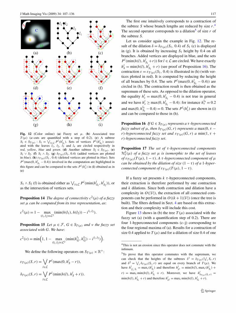
Fig. 12 (Color online) (a) Fuzzy set μ. (b) Associated treeT (μ) (α-cuts are quantified with a step of 0.2). (c) A subtreeS1 ∈ ST (μ) : S1 = ∨

l∈L P l(hlS1

). Sets of vertices P l(hlS1

) associ-ated with the leaves l1, l2, l3 and l4 are circled respectively inred, yellow, blue and green. (d) Another subtree S2 ∈ ST (μ). (e)S1 ∨ S2. (f) S1 ∧ S2. (g) δT (μ)(S1, 0.4) (added vertices are plottedin blue). (h) εT (μ)(S1 , 0.4) (deleted vertices are plotted in blue). SetsP l(max(0, hl

S1− 0.4)) involved in the computation are highlighted in

this figure and can be compared to the sets P l(hlε) in (i) obtained as in

(c)

S1 ∧ S2 (f) is obtained either as∨

l∈L P l(min(hlS1

, hlS2

)), oras the intersection of vertices sets.

Proposition 14 The degree of connectivity c2(μ) of a fuzzyset μ can be computed from its tree representation, as:

c2(μ) = 1 − max(l1,l2)∈L2

(min(h(l1), h(l2)) − il1,l2).

Proposition 15 Let μ ∈ F , G ∈ ST (μ) and ν the fuzzy setassociated with G. We have:

c2(ν) = min(

1,1 − max(l1,l2)∈L2

(min(hl1G,h

l2G) − il1,l2)

).

We define the following operators on ST (μ) × R+:

εT (μ)(S, r) =∨

l∈LP l(max(0, hl

S − r)),

δT (μ)(S, r) =∨

l∈LP l(min(h(l), hl

S + r)).

The first one intuitively corresponds to a contraction ofthe subtree S whose branch lengths are reduced by size r .4

The second operator corresponds to a dilation5 of size r ofthe subtree S.

Let us consider again the example in Fig. 12. The re-sult of the dilation δ = δT (μ)(S1, 0.4) of S1 (c) is displayedin (g). It is obtained by increasing S1 height by 0.4 on allbranches. Added vertices are displayed in blue, and the setsP l(min(h(l), hl

S1+r)) for l ∈ L are circled. We have exactly

hlδ = min(h(l), hl

S1+ r) (see proof of Proposition 16). The

contraction ε = εT (μ)(S1, 0.4) is illustrated in (h) (with ver-tices plotted in red). It is computed by reducing the heightof all branches by 0.4. The sets P l(max(0, hl

S1− 0.4)) are

circled in (h). The contraction result is then obtained as thesupremum of these sets. As opposed to the dilation operator,the equality hl

ε = max(0, hlS1

− 0.4) is not true in general

and we have hlε ≥ max(0, hl

S1− 0.4): for instance h

l4ε = 0.2

and max(0, hl4S1

− 0.4) = 0. The sets P l(hlε) are shown in (i)

and can be compared to those in (h).

Proposition 16 If G ∈ ST (μ) represents a τ -hyperconnectedfuzzy subset of μ, then δT (μ)(G, r) represents a max(0, τ −r)-hyperconnected fuzzy set and εT (μ)(G, r) a min(1, τ +r)-hyperconnected fuzzy set.

Proposition 17 The set of τ -hyperconnected componentsH2

τ (μ) of a fuzzy set μ is isomorphic to the set of leavesof εT (μ)(T (μ),1 − τ). A τ -hyperconnected component of μ

can be obtained by the dilation of size (1 − τ) of a 1-hyper-connected component of εT (μ)(T (μ),1 − τ).

If a fuzzy set presents k τ -hyperconnected components,their extraction is therefore performed by one contractionand k dilations. Since both contraction and dilation have acomplexity in O(|V |), the extraction of all connected com-ponents can be performed in O((k + 1)|V |) (once the tree isbuilt). The filters defined in Sect. 4 are based on this extrac-tion and their complexity will include this cost.

Figure 13 shows in (b) the tree T (μ) associated with thefuzzy set (a) (with a quantification step of 0.2). There arefour 1-hyperconnected components (c–j) corresponding tothe four regional maxima of (a). Results for a contraction ofsize 0.4 applied to T (μ) and for a dilation of size 0.4 of one

4This is not an erosion since this operator does not commute with theinfimum.5To prove that this operator commutes with the supremum, wecan check that the heights of the subtrees δ1 = δT (μ)(

∨i Si , r)

and δ2 = ∨i δT (μ)(Si , r) are equal on every branch of T (μ). We

have hl∨i Si

= maxi (hlSi

) and therefore hlδ1 = min(h(l),maxi (h

lSi

) +r) = maxi min(h(l), hl

Si+ r). Moreover, we have hl

δT (μ)(Si ,r)=

min(h(l), hlSi

+ r) and therefore hlδ2 = maxi min(h(l), hl

Si+ r).


Fig. 13 (Color online) (a) Fuzzy set. (b) Associated tree (the α-cutsare quantified with a 0.2 step). The four 1-hyperconnected compo-nents (d), (f), (h) and (j) and associated subtrees (c), (e), (g) and(i). (k) Subtree corresponding to the contraction of size 0.4 (in ma-genta). (l) A 0.6-hyperconnected component (circled in red) ob-tained as the dilation of a 1-hyperconnected component of the con-traction (in magenta) and the corresponding fuzzy set (m). Another0.6-hyperconnected component (n) and the associated fuzzy set (o).(p) Number of τ -hyperconnected components of the fuzzy set (a) cor-rupted with white Gaussian noise (of variance 0.005) as function of τ

of the 1-hyperconnected components are illustrated respec-tively in (k) et (l). The resulting subtree corresponds exactlyto a 0.6-hyperconnected component (m) of μ. The second0.6-hyperconnected component is illustrated in (o) and itsassociated subtree in (n). If the fuzzy set (a) is corruptedwith white Gaussian noise of variance 0.05, we obtain about20,000 1-hyperconnected components. The evolution of thenumber of τ -hyperconnected components as a function of τ

is plotted in (p), illustrating the grouping effect.

4 Attribute Openings Applied to Fuzzy Sets

4.1 Motivation

We focus here on segmentation and recognition tasks. Inthis context we want to extract a connected object A rep-resented by its membership function μA. For this purpose,we rely on prior structural knowledge expressed as spatialrelations between structures [3], and on grey-level informa-tion. The segmentation and recognition process can thus beformalized as an iterative reduction of an over-estimationA of μA [27]. Considering a current over-estimation A anda prior on A represented as a characteristic function f onF , we can obtain a new upper-bound A

′as the supremum

of the fuzzy sets that fulfill the prior and that are smallerthan A: A

′ = ∨{ν ∈ F | ν ≤ A and f (ν) = 1}. As illus-trated in the sequel, such reductions can be performed basedon grey-level prior or on an approximate spatial location. Inthis framework, we can also take advantage of connectiv-ity priors about objects of interest. Considering the connec-tivity constraint and some available prior information aboutthe object, we want to obtain a reduction A

′of an over-

estimation A such that μA ≤ A′ ≤ A.

Figure 14 provides an example on a brain MRI segmen-tation and recognition task. Suppose for instance that wehave already extracted the brain surface and that we wantto extract the right lateral ventricle LV r delineated in red(a) on one axial slice of a 3D T1 weighted brain MRI. Fromgrey-level prior we can obtain a first over-estimation LV rGl ,since the lateral ventricles have darker intensities than otherbrain tissues, including white matter and grey matter, on thistype of images. Lateral ventricles are also always quite cen-tral in the brain. This prior can be translated into a fuzzy setLV rSp (c), so as to guarantee μLV r ≤ LV rSp . The conjunc-tive fusion LV r = LV rGl ∧LV rSp is shown in (d), and sat-isfies μLV r ≤ LV r . Although the over-estimation has beenstrongly reduced, LV r still exhibits several connected com-ponents. The circled ones, for instance, correspond to brainsulci and present a volume smaller than the typical rangeof volume for the lateral ventricle in normal cases. We canthus remove the connected components of LV r that do notfulfill a minimal volume criterion (based on a prior volumeinformation for the lateral ventricle).


Fig. 14 (a) One axial slice of a 3D brain MRI. (b) Grey level infor-mation: LV rGl . (c) Central location inside the brain: LV rSp . (d) Con-junctive fusion

4.2 Attribute Openings Based on a Crisp Criterion

We first suppose that some prior knowledge about the con-nected object A is expressed as a crisp criterion function:fC : F → {0,1} such that fC(μA) = 1. Based on fC , wedefine the following operator on F :

ξ(A) =∨

{ν ∈ H2τ |ν ≤ A and fC(ν) = 1}. (5)

This operator satisfies the property μA ≤ ξ(A) ≤ A, sinceμA is supposed to be connected, to be smaller than A andto fulfill the criterion. The resulting fuzzy set is thus a betterapproximation of μA than A. It is important to note that thisoperator is increasing, idempotent and anti-extensive and isthus a morphological opening.

However without any condition on fC , the computationof this operator requires to evaluate the criterion over all el-ements of H2

τ smaller than A and has an exponential com-plexity. To overcome this, we take advantage of the fol-lowing property: ∀ν ∈ H2

τ , ν ≤ A ⇒ ∃μi ∈ H2τ (A), ν ≤ μi .

Therefore if the criterion fC is increasing, the computationof ξ(A) can be performed over the τ -hyperconnected com-ponents of A:

ξ(A) =∨

{μi ∈ H2τ (A)|fC(μi) = 1}. (6)

This filter only processes connected components of A andcorresponds intuitively to an extension of attribute openingsas defined for binary images [8, 13]. Note that the increas-ingness of the criterion is required to obtain a tractable com-putation of (5), which prevents using non increasing criteriasuch as shape criteria as recently proposed in [44].

This filter can be easily computed using the tree repre-sentation. Proposition 17 ensures an isomorphism between

Fig. 15 Algorithm used to compute ξ(A)

the leaves of εT (A)(T (A),1 − τ) and the τ -hyperconnected

components of A. The process can thus be efficiently per-formed with the algorithm described in Fig. 15, where themost time consuming operation is the tree computation [25].

More precisely, the complexity of this filter is in O((k +1)|V | + kCfC

+ CT ), where CT is the cost of the tree com-putation, CfC

is the cost of the criterion computation andk is the cardinality of H2

τ (A). Computing the criterion canbe computationally expensive since it has to be performed k

times and it generally involves a computation over all ver-tices of the τ -hyperconnected components (a vertex can be-long to more than one τ -hyperconnected component anda pixel to more than one vertex). However, a preliminarypartial computation of the criterion can sometimes be per-formed during the tree computation. For instance if we con-sider an area criterion (the area of a fuzzy set μ is definedas S(μ) = ∑

x∈X μ(x)), it can be advantageous to compute,during the tree initialization, the area associated with everyvertex of the tree. The area of the τ -hyperconnected compo-nents is then obtained as the sum of vertices area, that werepreviously computed.

Figure 16 presents an example, where the criterion isdefined as a minimal area of 10,000 pixels and the cho-sen hyperconnection is H2

0.6. During the computation ofthe tree (b) associated with the fuzzy set (a), we com-pute for each vertex its associated area. We then computeεT (μ)(T (μ),0.4) to obtain the 0.6-hyperconnected compo-nents (c) and (d). Their areas are respectively 8612 and11,520 pixels and can be easily obtained from the verticesarea. The first one does not satisfy the criterion. The secondone does and is the resulting subtree in this case (d) whichrepresents the fuzzy set (e).

4.3 Extension to a Fuzzy Criterion

The filter proposed in the previous section only handles crispcriteria. It follows that it is not continuous since a smallmodification of the input set may result in the modificationof a complete connected component. To overcome this andachieve more robustness in the filtering process, we extendin this section the previous definition to fuzzy criteria. For


Fig. 16 Fuzzy set (a) and its representation as a tree (b) (the verticesare labeled with their area). Two 0.6-hyperconnected components (c)and (d). The area of the component (c) is smaller than the minimalthreshold. This component does not belong to the result, whereas thecomponent (d) does. (e) Resulting fuzzy set

instance, a minimal area criterion can be represented by amembership function (corresponding for instance to a lin-guistic value such as “large”). The satisfaction of the crite-rion by a fuzzy set ν is thus defined as a degree μC(ν).

We propose to preserve connected fuzzy subsets whosemaximum membership degree is less than or equal to thesatisfaction degree of the criterion via the following operator(which guarantees the idempotence of the associated filter):

ξμC(A) =

∨{ν ∈ H2

τ | ν ≤ A and maxx∈X

ν(x) ≤ μC(ν)}.

(7)

This operator is also a morphological opening and re-duces to (5) if μC is crisp. If it is not crisp but Lipschitz, itpresents nice regularity properties expressed by the follow-ing proposition (regularity properties given in the followingmake the assumption that the membership degrees are notquantified).

Proposition 18 If μC is Lipschitz, then the mapping asso-ciating A with ξμC

(A) is Lipschitz.

For computational purposes, we also assume that μC isincreasing which leads to a simplification of (7).6

Proposition 19 If μC is increasing, ξμC(A) rewrites as:

6Note that if μC(ν) is increasing for fixed maxx∈X ν(x), Proposition 19still holds.

Fig. 17 (Color online) (a) Fuzzy set. Two 0.6-hyperconnected com-ponents (b) and (c). (d) μS in red plain, in dashed blue the values(S(min(μi,m)),m). Resulting subtree (e) and associated fuzzy set (f).See Table 2 for detailed values involved in this filtering process

ξμC(A) =

∨

μi∈H2

τ (A)

∨

m∈[0,1]{min(μi,m) | m ≤ μC(min(μi,m))}.

This leads to a fast computation of ξμC(A) since we only

have to handle the τ -hyperconnected components “leveled”at m (i.e. min(μi,m)). Therefore this filter has a complexity

in O((k + 1)|V | + kCfC

s+ CT ), where CT is the cost of the

tree computation, CfCis the cost of the criterion computa-

tion, k is the cardinal of H2τ (A) and s is the quantification

step of the membership degrees.We illustrate this definition in Fig. 17. The criterion is

here defined as a membership function μS : R+ → [0,1]

(d) representing a fuzzy minimal threshold on the area(computed as the cardinality of the fuzzy set: S(μ) =∑

x∈X μ(x)). First we extract from the tree (b) (which repre-sents the fuzzy set μ (a)) the two 0.6-hyperconnected com-ponents μ1 (b) and μ2 (c). These components are then pro-gressively leveled from 1 to 0: ν = min(μi,m). The satisfac-tion degree of the criterion μS(S(ν)) is evaluated for eachleveled subtree. If the level is less than or equal to this de-gree we add the leveled subtree to the resulting subtree (e).The associated fuzzy set is shown in (f). Table 2 shows forthe two 0.6-hyperconnected components and all levels m,the area of leveled subtree, the satisfaction degree of the cri-terion μS and finally whether the leveled subtree has to beadded to the result or not.

5 Filtering

We propose in this section two connected filters, based onthe definitions introduced in Sect. 4, that can be used ina segmentation and recognition process, implementing theidea of deriving a finer estimation of μA from a first roughover-estimation A and a criterion.


Table 2 For each connected component presented in Fig. 17 and foreach level m, the area of the thresholded component: min(μi,m), thesatisfaction degree μS(S(ν)) and the satisfaction of the criterion C:maxx∈X ν(x) ≤ μS(S(ν)) are provided

Connected component (b) Connected component (c)

Level S(ν) μS(S(ν)) C S(ν) μS(S(ν)) C

1 8612 0.7687 no 11520 1 yes

0.8 8411 0.7352 no 11267 1 yes

0.6 8163 0.6938 yes 10056 1 yes

0.4 7880 0.6467 yes 7880 0.6467 yes

0.2 4554 0.0923 no 4554 0.0923 no

0 0 0 yes 0 0 yes

5.1 Marker Inclusion

We define a criterion from another estimation A of μA, suchthat A ≤ μA (A can be seen as a marker7 of the target ob-ject):

ξ1A(A) =

∨{ν ∈ H2

τ |ν ≤ A and A ≤ ν}. (8)

Figure 18 illustrates this filter on a 1D example and forτ = 1. The fuzzy set A (a) in blue is filtered by various mark-ers A (b–f) in dashed red. In (b) only one hyperconnectedcomponent fulfills the inclusion constraint and is preserved.In (c) and (d), two hyperconnected components satisfy theinclusion constraint. A small modification of the markerleads in (e) to the satisfaction of the constraint with thefour connected components. As the height of the marker de-creases, the connectivity degree of the result also decreases.This property will be formally expressed by Proposition 20.In addition, discontinuities appear as A changes (considerfor instance (d) and (e)), which illustrates that ξ1

A is not con-tinuous with respect to A. In (f) the marker A cannot beincluded in any hyperconnected component of A (since thechosen connectivity degree τ = 1 is too strict) and the filterthus returns an empty set.

Proposition 20 Let α = maxx∈X A(x). The result of the fil-ter defined in (8) is max(0, (α − (1 − τ)))-hyperconnected.

Instead of considering a strict inclusion, we can rely on afuzzy one, based on Lukasiewicz operator [10]:

μ≤(μA,μB) = minx∈X

min(1,1 − μA(x) + μB(x)).

The filter defined by (7) then writes:

ξ2A(A) =

∨{ν ∈ H2

τ | ν ≤ A and maxx∈X

ν(x) ≤ μ≤(A, ν)}.

(9)

7Note that this filter does not behave as a reconstruction filter.

Fig. 18 (Color online) Filtering of a fuzzy set A (a) according to (8)using markers A (in red) of decreasing height (b–e) or a marker A thatpresents two distinct modes (f). The result is displayed in blue. In (f),the result is 0F (meaning that there is actually no solution satisfyingthe constraints)

Fig. 19 (Color online) Filtering of a fuzzy set A (a) according to (9)(for τ = 1) using markers A (in red) of decreasing height (b–e) or amarker A that presents two distinct modes (f). The result is displayedin blue

The results of this filter are presented in Fig. 19 (forτ = 1) and can be compared to the results in Fig. 18. Wecan notice that the input fuzzy set is now progressively fil-tered when the marker gets larger and larger. Intuitively, hy-perconnected components verifying the inclusion constraintare kept, while the other ones are reduced to a level corre-sponding to the degree of satisfaction of the constraint.

Proposition 21 The mapping associating A with ξ2A(A) is

Lipschitz, as well as the mapping that associates A to ξ2A(A).

Proposition 22 Let α = maxx∈X A(x). The result of theconnected filter defined in (9) is max(0, (α − (1 − τ)))-hyperconnected.

We illustrate now this filter on a brain recognition task inFig. 20. As in Sect. 4.1, we want to extract the right lateralventricle from a brain MRI (a). We will refine the overes-timation LV r (b) obtained in Fig. 14(d) based on a marker


Fig. 20 (a) One axial slice of a 3D brain MRI. (b) LV r . (c–f) Resultsof the connected filter specified by (9) using a marker centered in theright ventricle, with maximal value 1, 0.75, 0.5 and 0, respectively

LV r defined as a fuzzy set having a support reduced to onepoint centered in the right lateral ventricle, with a member-ship value taking values 1 (which mostly selects the rightventricle), 0.75, 0.5 and 0 (which does not filter), respec-tively (c–f). In (c) the right lateral ventricle is clearly dis-tinguished from the other parts of the fuzzy set in (b). Thisdistinction decreases with the maximal value of the markerand the other parts of the fuzzy set have higher and highermembership degrees in the filtering result. A potential ap-plication of this approach is to perform a filter, preservingconnectivity properties, and being more or less selective de-pending on the confidence we may have in the marker.

5.2 Fuzzy Area Opening

Area opening is a well known connected operators [45]. Itfilters connected components based on a minimal area crite-rion, and can be formulated as:

ξSmin(A) =∨

{c ∈ C | c ≤ A and S(c) ≥ Smin},where C is a connection over X and S a function computingthe area. In the examples developed in Sect. 4, we used acriterion based on the area defined as the cardinality of thefuzzy objects. We denote by ξ1

Sminthe filter derived from (5)

using a crisp minimal area criterion, and by ξ2μSmin

the filterderived from (7) using a fuzzy minimal area criterion.

However modeling the area of the fuzzy set by its car-dinality is quite simplistic (think for instance of a fuzzy setthat has a large support and a small kernel) and it may bemore appropriate to consider a criterion on the area of eachα-cut. To this aim we make use of the following fuzzy mea-sure of the area [10]: μS(μ)(s) = supS(μα)≥s α, which rep-resents the highest level such that all α-cuts of μ until thislevel have an area larger than s. The membership functionμS(μ) is decreasing. If we consider a minimal area Smin,

the inequality maxx∈X ν(x) ≤ μS(ν)(Smin) is therefore ful-filled if all non empty α-cuts of ν satisfy the area criterion.Deriving the filter of (7), we obtain:

ξ2Smin

(A) =∨{

ν ∈ H2τ | ν ≤ A and

maxx∈X

ν(x) ≤ μS(ν)(Smin)}.

For more flexibility in recognition tasks, it is more appro-priate to represent the criterion by a membership functionμSmin : R

+ → [0,1] (for instance a ramp function replac-ing the crisp threshold). We will now keep fuzzy sets whoseheight is smaller than the satisfaction degree μSmin(sm),where sm is the area of its highest non empty α-cut. Thisproperty can be expressed as the satisfaction of the inequal-ity

maxx∈X

ν(x) ≤ maxs∈R+ min(μS(ν)(s),μSmin(s)).

The filter defined by (7) then rewrites:

ξ2μSmin

(A) =∨{

ν ∈ H2τ | ν ≤ A and

maxx∈X

ν(x) ≤ maxs∈R+ min(μS(ν)(s),

μSmin(s))}.

Figure 21 illustrates these filters for τ = 1. The fuzzy set(a) contains 7 objects of increasing area. Their fuzzy areaμS(μ) is represented in (b) and their area (defined as thecardinality of the fuzzy set) is respectively 60.77, 281.57,669.44, 1202.12, 1896.76, 2696.83 and 3702.12. We firstapply the filter ξ1

Smin(based on a minimal value of the car-

dinality) with Smin = 1202 (c) and Smin = 1203 (d). In (c)three objects are filtered whereas in (d) there are four. Thisillustrates that this filter is not continuous according to theparameter Smin. In (e) we apply ξ2

Sminwith Smin = 1202. All

α-cuts of the 1-hyperconnected components that satisfy thecriterion are selected and the third object is now partially fil-tered. The use of a membership function μSmin (b) (in dashedred) as criterion leads to more robustness of the filter. Theresult ξ2

μSminis presented in (f).

Proposition 23 The mapping that associates A to ξ2μSmin

(A)

is Lipschitz, as well as the mapping that associates μSmin toξ2μSmin

(A).

Figure 22 illustrates this filter on a brain MRI example.We filter an over-estimation LV r of the lateral ventricles (b)according to a minimal volume prior represented by a mem-bership function μSmin . The result ξ2

μSmin(LV r) is shown

in (c). Some components corresponding in particular to thesulci are efficiently removed and we thus obtain a better ap-proximation of the lateral ventricles.


Fig. 21 (Color online) (a) Fuzzy set that contains 7 objects of increas-ing size. (b) For each object, fuzzy area μS(μ)(s) in blue and a mini-mal fuzzy threshold μSmin in dashed red. Filtering of (a) by ξ1

1202 (c),ξ1

1203 (d), ξ21202 (e) and ξ2

μSmin(f)

Fig. 22 (a) One axial slice of a 3D MRI. (b) LV r . (c) ξ2μSmin

(LV r)

6 Conclusion

In this paper, we focused on the notion of connectivity offuzzy sets. The contributions are three-fold. From a theo-retical point of view, we proposed a new definition of ameasure of connectivity, represented as a family of hyper-connections and adapted to the semantics of fuzzy sets. Wederived a number of properties showing that some draw-backs of previously proposed measures are overcome. Froman algorithmical point of view, an efficient computationalframework was developed, based on a max-tree represen-tation of the considered fuzzy set. In this framework thehyperconnected-components can be easily identified and ex-tracted in linear time with respect to the number of vertices,once the tree is built. This leads to derived attribute open-ings, based on crisp or fuzzy criteria that presents also niceregularity properties. Finally, from an application point ofview, some hints on the potential of the proposed approachare illustrated on a brain imaging segmentation and recogni-tion task. The proposed connected openings based on mark-ers or on volume criteria lead to interesting gradual filteringand are used to refine a first approximation of specific brainstructures.

Future work aims at further developing such filters, andintegrating them in a segmentation framework in both nor-mal and pathological cases, as suggested in [26]. From a

more conceptual and theoretical point of view, another per-spective of this work concerns the combination of differ-ent structural criteria, including connectivity ones, in a con-straint network in order to drive a segmentation and recog-nition process [27].

Appendix: Proofs of the Main Results

Proof of Proposition 3 We will first prove that if xi belongsto a regional maximum Rμ of μ, then η1

δμ(xi )xi

(μ) ∈ H1. By

definition η1

δμ(xi )xi

(μ) = ∨{ν ∈ H1 | δμ(xi )xi

≤ ν ≤ μ}. Let us

show that all elements ν ∈ H1 satisfying δμ(xi)xi

≤ ν ≤ μ

overlap according to ⊥1.First let us show that maxx∈X ν(x) = μ(xi). According to

Proposition 2, if ν ∈ H1, ν has a unique regional maximum.Let xm be a point belonging to this regional maximum. Sincethis maximum is unique and X is bounded and discrete, forall points x ∈ X, there exists an increasing discrete path inν from x to xm. Thus there exists an increasing path lxi ,xm

in ν from xi to xm. Since ν(xi) = μ(xi) and ν ≤ μ, weobtain ∀xk ∈ lxi ,xm, μ(xk) ≥ ν(xk) ≥ μ(xi). Since lxi ,xm isincreasing, ∀xk ∈ lxi ,xm, xk ∈ Rμ (otherwise the first pointxk not belonging to Rμ would satisfy μ(xk) < μ(xi)). Thepoint xm thus belongs to Rμ and μ(xi) = μ(xm). There-fore ν reaches its global maximum at xi and all elementsν of H1 such that δ

μ(xi)xi

≤ ν ≤ μ satisfy ν(xi) = μ(xi) andmaxx∈X ν(x) = μxi

. They overlap according to ⊥1 (sincewhatever the level α, their α-cuts are either empty or con-tain xi and so intersect in xi ) and we obtain η1

δμ(xi )xi

(μ) ∈ H1.

Let us now prove that ∀x ∈ X, η1

δμ(xi )xi

(μ)(x) = c1μ(x, xi).

Let c be a fuzzy set such that ∀x ∈ X, c(x) = c1μ(x, xi).

Then c belongs to H1. Indeed, by definition, ∀α ∈ [0,1],(c)α = {x ∈ X | c1

μ(x, xi) ≥ α}. Let x be a point in (c)α andlx,xi

be a discrete path that maximizes the criterion:

maxl∈Lx,xi


0≤k≤nμ(xk).

We have ∀xk ∈ lx,xi, xk ∈ (c)α (since minxk∈lx,xi

μ(xk) ≥ α).For all pairs of points belonging to (c)α , there exists a dis-crete path in (c)α between those points that contains thepoint xi . We thus have ∀α ∈ [0,1], (c)α ∈ Cd and accordingto Proposition 1, c ∈ H1. In addition c(xi) = c1

μ(xi, xi) =μ(xi). Therefore c satisfies c ∈ H1 and δ

μ(xi)xi

≤ c ≤ μ. Wederive η1

δμ(xi )xi

(μ) ≥ c.

Let ν be in H1 such that δμ(xi )xi

≤ ν ≤ μ. Thus we have∀(x, y) ∈ X2, c1

ν(x, y) = min(ν(x), ν(y)). Since c1h(x, y) is


increasing according to h and ν ≤ μ, we obtain c1μ(x, y) ≥

min(ν(x), ν(y)). If we choose y = xi , we obtain c1μ(x, xi) ≥

min(ν(x), ν(xi)) and since ν(x) ≤ ν(xi) (see the first part ofthis proof), the property c ≥ ν is fulfilled for all elements ν

that belong to H1 and such that δμ(xi)xi

≤ ν ≤ μ. Thereforewe have η1

δμ(xi )xi

(μ) ≤ c, which completes the proof. �

Proof of Proposition 5 Let xm be a point for which theglobal maximum of μ is reached. Since X is bounded andfinite, the existence of xm is guaranteed. We want to provethat:

∀(x, y) ∈ X2, c2μ(x, y) ≥ min(c2

μ(x, xm), c2μ(y, xm)).

Let x and y be any two points in X. By definition:

c2μ(x, y) = 1 − min(μ(x),μ(y)) + c1

μ(x, y)

≥ 1 − min(μ(x),μ(y))

+ min(c1μ(x, xm), c1

μ(xm,y))

(since c1μ is max-min transitive)

≥ min(1 − min(μ(x),μ(y)) + c1μ(x, xm),

1 − min(μ(x),μ(y)) + c1μ(xm,y))

≥ min(1 − min(μ(x),μ(xm)) + c1μ(x, xm),

1 − min(μ(xm),μ(y)) + c1μ(xm,y))

(since μ(xm) ≥ max(μ(x),μ(y)))

≥ min(c2μ(x, xm), c2

μ(xm,y)). �

Proof of Proposition 6 Let μ ∈ F . We want to show thatc2μ(x, y) reaches its minimum for x being a point for which

the global maximum of μ is reached and y belonging to aregional maximum of μ. Let xm be a point for which theglobal maximum of μ is reached. Proposition 5 guaranteesthat:

∀(x, y) ∈ X2, c2μ(x, y) ≥ min(c2

μ(x, xm), c2μ(y, xm)).

We thus have:

min(x,y)∈X2

c2μ(x, y) ≥ min

x∈Xc2μ(x, xm),

and since xm ∈ X :min

(x,y)∈X2c2μ(x, y) = min

x∈Xc2μ(x, xm).

This proves that c2μ(x, y) reaches its minimum for x or y

being a point for which the global maximum of μ is reached.Let us now show that if xm is a point for which the global

maximum of μ is reached, then c2μ(xm,x) reaches its mini-

mum for x belonging to a regional maximum of μ. Let x be

any point in X. Let xi be a point that belongs to a regionalmaximum of μ such that there exists an increasing digitalpath from x to xi in μ (we have in particular μ(x) ≤ μ(xi)).The existence of this local maximum is guaranteed since X

is bounded and finite. We have to prove that:

c2μ(x, xm) ≥ c2

μ(xi, xm), or equivalently

c1μ(x, xm) − μ(x) ≥ c1

μ(xi, xm) − μ(xi), or

c1μ(x, xm) + μ(xi) ≥ c1

μ(xi, xm) + μ(x).

Let us prove the last inequality. Since c1μ is max-min tran-

sitive, we have:

c1μ(x, xm) ≥ min(c1

μ(x, xi), c1μ(xi, xm)). (10)

• If c1μ(xi, xm) ≥ c1

μ(x, xi):

10 ⇒ c1μ(x, xm) ≥ c1

μ(x, xi)

⇒ c1μ(x, xm) ≥ μ(x)

(there exists an increasing path

in μ from x to xi)

⇒ c1μ(x, xm) + μ(xi) ≥ c1

μ(xi, xm) + μ(x)

(since μ(xi) ≥ c1μ(xi, xm)).

• If c1μ(x, xi) ≥ c1

μ(xi, xm):

10 ⇒ c1μ(x, xm) ≥ c1

μ(xi, xm).

As c1μ is max-min transitive, we have:

c1μ(xi, xm) ≥ min(c1

μ(xi, x), c1μ(x, xm))

≥ min(μ(x), c1μ(x, xm))

≥ c1μ(x, xm).

Therefore we obtain:

c1μ(x, xm) = c1

μ(xi, xm)

⇒ c1μ(x, xm) + μ(xi) ≥ c1

μ(xi, xm) + μ(x)

since μ(xi) ≥ μ(x).

The property c1μ(x, xm) + μ(xi) ≥ c1

μ(xi, xm) + μ(x) istherefore always fulfilled and thus:

∀x ∈ X, c2μ(x, xm) ≥ c2

μ(xi, xm),

where xi belongs to a regional maximum of μ and xm to aglobal maximum of μ. �

Proof of Proposition 7 We first show that the mapping as-sociating c1

μ(x, y) with μ is Lipschitz for any fixed points


x and y. Let μA and μB be two fuzzy sets and η =dF (μA,μB). We want to prove that dF

X2 (c1μB

, c1μA

) ≤ η

(where dFX2 (f1, f2) = sup(x,y)∈X2 |f1(x, y) − f2(x, y)|).

Let x and y be any two points in X. Let LA andLB be two paths from x to y such that c1

μA(x, y) =

minxi∈LA μA(xi) and c1μB

(x, y) = minxi∈LB μB(xi) (sinceX is bounded and finite, the existence of those paths is guar-anteed). In addition dF (μA,μB) = η ⇒ ∀z ∈ X, |μA(z) −μB(z)| ≤ η. Let xa be a point in LA such thatminxi∈LA μA(xi) = μA(xa) and xb be a point in LA suchthat minxi∈LA μB(xi) = μB(xb). As dF (μA,μB) = η, wehave:{ |μA(xa) − μB(xa)| ≤ η,

|μA(xb) − μB(xb)| ≤ η

⇒{−η + μB(xa) ≤ minxi∈LA μA(xi) ≤ η + μB(xa),

−η + μA(xb) ≤ minxi∈LA μB(xi) ≤ η + μA(xb)

⇒{−η + minxi∈LA μB(xi) ≤ minxi∈LA μA(xi),

−η + minxi∈LA μA(xi) ≤ minxi∈LA μB(xi)

⇒∣∣∣ minxi∈LA

μA(xi) − minxi∈LA

μB(xi)

∣∣∣ ≤ η.

In the same way we derive:∣∣∣ minxi∈LB

μA(xi) − minxi∈LB

μB(xi)

∣∣∣ ≤ η.

So:{ |minxi∈LB μA(xi) − minxi∈LB μB(xi)| ≤ η,

|minxi∈LA μA(xi) − minxi∈LA μB(xi)| ≤ η

⇒{ |minxi∈LB μA(xi) − c1

μB(x, y)| ≤ η,

|c1μA

(x, y) − minxi∈LA μB(xi)| ≤ η

⇒{

c1μB

(x, y) ≤ minxi∈LB μA(xi) + η,

c1μA

(x, y) ≤ minxi∈LA μB(xi) + η.

The definition of c1μ guarantees that:

{minxi∈LB μA(xi) ≤ c1

μA(x, y),

minxi∈LA μB(xi) ≤ c1μB

(x, y),

from which we derive, ∀(x, y) ∈ X2:

{c1μB

(x, y) ≤ c1μA

(x, y) + η,

c1μA

(x, y) ≤ c1μB

(x, y) + η

⇒ |c1μB

(x, y) − c1μA

(x, y)| ≤ η.

Therefore we obtain dFX2 (c

1μB

, c1μA

) ≤ η and the mapping

associating c1μ(x, y) with μ is Lipschitz.

Let us now prove that the mapping associating c2μ(x, y)

with μ is 2-Lipschitz for given x and y. Let μA and μB be

two fuzzy sets, η = dF (μA,μB) and (x, y) ∈ X2. Since c1μ

is Lipschitz:

|c1μB

(x, y) − c1μA

(x, y)| ≤ η

⇒ −η + c1μB

(x, y) ≤ c1μA

(x, y) ≤ η + c1μB

(x, y). (I1)

In addition:

∀z ∈ X, |μA(z) − μB(z)| ≤ η

⇒ ∀z ∈ X,−η + μB(z) ≤ μA(z) ≤ η + μB(z)

⇒{−η + μB(x) ≤ μA(x) ≤ η + μB(x),

−η + μB(y) ≤ μA(y) ≤ η + μB(y)

(for z = x and z = y respectively)

⇒{−η + min(μB(x),μB(y)) ≤ min(μA(x),μA(y)),

min(μA(x),μA(y)) ≤ η + min(μB(x),μB(y))

⇒

⎧⎪⎪⎨

⎪⎪⎩

1 − η − min(μB(x),μB(y))

≤ 1 − min(μA(x),μA(y)),

1 − min(μA(x),μA(y))

≤ 1 + η − min(μB(x),μB(y))

⇒

⎧⎪⎪⎨

⎪⎪⎩

−2η + 1 − min(μB(x),μB(y)) + c1μB

(x, y)

≤ 1 − min(μA(x),μA(y)) + c1μA

(x, y),

1 − min(μA(x),μA(y)) + c1μA

(x, y)

≤ 2η + 1 − min(μB(x),μB(y)) + c1μB

(x, y)

(adding (I1) and (I2))

⇒ |c2μA

(x, y) − c2μB

(x, y)| ≤ 2η. (I2)

Consequently the mapping associating μ with c2μ(x, y) is

2-Lipschitz. �

Proof of Proposition 8 We show that the mapping c2(μ)

is 2-Lipschitz. Let μA and μB be two fuzzy sets andη = dF (μA,μB). Let xA and yA be two points in X suchthat c2(μA) = c2

μA(xA, yA) and (xB, yB) ∈ X2 such that

c2(μB) = c2μB

(xB, yB).As c2

μ is 2-Lipschitz:

{ |c2μA

(xA, yA) − c2μB

(xA, yA)| ≤ 2η,

|c2μA

(xB, yB) − c2μB

(xB, yB)| ≤ 2η

⇒{

c2μB

(xA, yA) ≤ 2η + c2μA

(xA, yA),

c2μA

(xB, yB) ≤ 2η + c2μB

(xB, yB)

⇒{

c2μB

(xA, yA) ≤ 2η + c2(μA),

c2μA

(xB, yB) ≤ 2η + c2(μB)

⇒{

c2(μB) ≤ 2η + c2(μA),

c2(μA) ≤ 2η + c2(μB)


(as c2(μB) ≤ c2μB

(xA, yA) and

c2(μA) ≤ c2μA

(xB, yB))

⇒ −2η + c2(μB) ≤ c2(μA) ≤ 2η + c2(μB)

⇒ |c2(μA) − c2(μB)| ≤ 2η.

The mapping c2 is therefore 2-Lipschitz. �

Proof of Proposition 9 To prove that H2τ is a hyperconnec-

tion on F for the overlap mapping ⊥2τ , we have to show

that:

– 0F ∈ H2τ ,

– H2τ contains a sup-generating family S of F ,

– for any family {μi} of elements of H2τ such that

⊥2τ ({μi}) = 1, then

∨

i

μi ∈ H2τ .

(1) As ∀(x, y) ∈ X2 , c10F

(x, y) = 0, we have ∀(x, y) ∈X2, c2

0F(x, y) = 1 and thus c2(0F ) = 1. This shows that

∀τ ∈ [0,1],0F ∈ H2τ .

(2) ∀x ∈ X, ∀t ∈ [0,1], c2(δtx) = 1 and so ∀x ∈ X, ∀t ∈

[0,1], ∀τ ∈ [0,1], δtx ∈ H2

τ . In addition the family{δt

x | x ∈ X, t ∈ [0,1]} is sup-generating in F .(3) Let {μi} be a family of elements of H2

τ such that⊥2

τ ({μi}) = 1. We denote by μ the supremum of thisfamily: μ = ∨

i μi . We have to show that c2(μ) ≥ τ .

Let xm be a point for which the global maximum of μ

is reached, μm be an element of the family {μi} such thatμ(xm) = μm(xm) and y be a point that belongs to a regionalmaximum of μ such that c2(μ) = 1−μ(y)+ c1

μ(xm,y) (theexistence is guaranteed by Proposition 6). Let k be such thatμk(y) = μ(y), then:

c2(μ) = 1 − μk(y) + c1μ(xm,y).

As c1μ is max-min transitive we have:

c1μ(xm,y) ≥ min(c1

μ(xm,xk), c1μ(xk, y)), (11)

where xk is a point for which the global maximum of μk isreached.

⊥2τ ({μi}) = 1

⇒ ∀α ∈ [0,1],⋂

i

{(η1δhixi

(μi))α | α ≤ hi − 1 + τ } �= ∅

where hi = maxx∈X

μi(x) = μi(xi)

⇒ ∀α ∈ [0,1], α ≤ min(μm(xm),μk(xk)) − 1 + τ,

(η1δhmxm

(μm))α ∩ (η1δhkxk

(μk))α �= ∅

(considering only indices associated

with μk and to μm)

⇒ ∃l ∈ Lxk,xm, l = {x0 = xk, x1, . . . , xn = xm}such that min

0≤i≤n

(η1

δhkxk

(μk) ∨ η1δhmxm

(μm))(xi)

≥ min(μm(xm),μk(xk)) − 1 + τ,

where Lxk,xm is the set of discrete paths from xk to xm, ac-cording to the discrete connectivity cd defined on X. Indeedaccording to Proposition 3, η1

δhkxk

(μk) ∈ H1 and η1δhmxm

(μm) ∈H1 and so according to Proposition 1, all their α-cuts areconnected in the sense of the discrete connectivity cd . If wechoose α0 = min(μm(xm),μk(xk)) − 1 + τ , the α-cuts ofη1

δhkxk

(μk) and of η1δhmxm

(μm)(xi) at level α0 are connected and

intersect. Their union is thus connected. This guarantees theexistence of the path l. Since

c1μ(x, y) = max

l∈Lx,y


0≤i≤nμ(xi),

we obtain:

c1η1

δhkxk

(μk)∨η1

δhmxm

(μm)(xm, xk) ≥ μk(xk) − 1 + τ

⇒ c1μ(xm,xk) ≥ μk(xk) − 1 + τ

(as c1μ is increasing according to μ)

⇒ c1μ(xm,xk) ≥ μk(y) − 1 + τ

(as μk(xk) ≥ μk(y)).

In addition:

μk ∈ H2τ

⇒ c2(μk) ≥ τ

⇒ 1 − min(μk(xk),μk(y)) + c1μk

(xk, y) ≥ τ

(since ∀(x1, x2) ∈ X2 , c2μk

(x1, x2) ≥ c2(μk))

⇒ 1 − μk(y) + c1μk

(xk, y) ≥ τ

⇒ c1μk

(xk, y) ≥ μk(y) − 1 + τ

⇒ c1μ(xk, y) ≥ μk(y) − 1 + τ

(as c1μ is increasing according to μ).


11 ⇒ c1μ(xm,y) ≥ min(c1

μ(xm,xk), c1μ(xk, y))

⇒ c1μ(xm,y) ≥ μk(y) − 1 + τ


Fig. 23 A 1D fuzzy set μ. μR

associated with a regionalmaximum. ν1 belongs to H1

and μR ≤ ν1. ν2 /∈ H1

⇒ 1 − μk(y) + c1μ(xm,y) ≥ τ

⇒ 1 − μ(y) + c1μ(xm,y) ≥ τ

(as μ(y) = μk(y))

⇒ 1 − min(μ(xm),μ(y)) + c1μ(xm,y) ≥ τ

(as μ(y) ≤ μ(xm))

⇒ c2(μ) ≥ τ

⇒ μ ∈ H2τ . �

Proof of Proposition 11 According to Proposition 3, if xi

belongs to a regional maximum of μ, then η1

δμ(xi )xi

∈ H1 and

Proposition 10 guarantees that η1

δμ(xi )xi

∈ H1(μ).

We still have to prove that the set of 1-hyperconnectedcomponents H1(μ) of μ according to H1 is isomorphic tothe regional maxima {Ri} of μ. To this aim let us show thatthe elements of H1(μ) are exactly the connected openingsη1

μRwhose origins are associated with the regional maxima

of μ. Let R ⊆ X be a regional maximum of μ. Let μR(x) =μ(x) = hR if x ∈ R and 0 otherwise, hR being the height ofthis fuzzy set. Let us show that η1

μR(μ) belongs to H1(μ)

and that the mapping η1μR

(μ) : {Ri} → H1(μ) is bijective.The connected opening of origin μR can be expressed as:

η1μR

(μ) = ∨{ν ∈ H1 | μR ≤ ν ≤ μ}. The set of elements ν

that fulfills those conditions intersect (at least) for all lev-els α ∈ [0, hR] since all of them include μR . In addition allthose elements are such that maxx∈X ν(x) = hR (cf. proofof Proposition 3). Indeed otherwise the set ν would haveat least two regional maxima and would not belong to H1

(Fig. 23 illustrates the notations used here. ν2 is a fuzzyset such that maxx∈X ν2(x) > hR but ν2 /∈ H1). We canconclude that ⊥1({ν ∈ H1 | μR ≤ ν ≤ μ}) = 1 and there-fore that η1

μR(μ) ∈ H1. Proposition 10 then guarantees that

η1μR

(μ) ∈ H1(μ).Let us now show that the mapping η1

μR(μ) : {Ri} →

H1(μ) is surjective and thus that each 1-hyperconnectedcomponent of μ is associated with a regional maximumof μ. Let μi ∈ H1(μ) and xi be a point for which the globalmaximum of μi is reached (note that we have μi(xi) =μ(xi)). If xi belongs to a regional maximum Ri of μ, thenμi = η1

μRi(μ) and therefore μi is associated with Ri . Let

us assume that xi does not belong to a regional maximumof μ. Let xm belonging to a regional maximum of μ suchthat there exists an increasing path from xi to xm in μ.We consider the fuzzy set ν such that ν(x) = μ(x) for x

in that path and ν(x) = 0 otherwise. We can show that⊥1(μi, ν) = 1 and thus that μi ∨ ν ∈ H1. In addition theproperty μi < μi ∨ ν ≤ μ derives from definition of ν.This contradicts the property �ν ∈ H1,μi < ν ≤ μ (sinceμi ∈ H1(μ)). Therefore this case cannot occur et xi alwaysbelongs to a regional maximum of μ and μi = η1

μRi(μ).

We still have to prove that η1μR

(μ) : {Ri} → H1(μ) isinjective. Let Ri and Rj be two regional maxima of μ, μi =η1

μRi(μ) and μj = η1

μRj(μ). Let us assume that μi = μj .

This leads to μi ≥ μRi∨ μRj

. As μi ≤ μ and as Ri and Rj

are distinct regional maxima, μi has at least two regionalmaxima, which contradicts μi ∈ H1(μ). μi and μj are thusdistinct.

H1(μ) and the set of regional maxima of μ are thus iso-morphic. �

Proof of Proposition 12 Let μ be a fuzzy set andH1(μ) = {μi}. Proposition 11 guarantees that each μi isassociated with one regional maximum of μ. We denoteby xi a point that belongs to the regional maximum asso-ciated with μi and xj a point that belongs to the regionalmaximum associated with μj . Let us prove that:

c1μ(xi, xj ) = max

x∈Xmin(μi(x),μj (x)).

First we will show that:

c1μ(xi, xj ) ≥ max

x∈Xmin(μi(x),μj (x)).

The measure c1μ is max-min transitive and so:

c1μi∨μj

(xi, xj ) ≥ maxx∈X

min(c1μi∨μj

(xi, x), c1μi∨μj

(x, xj )).

In addition c1μi∨μj

(xi, x) ≥ c1μi

(xi, x), since c1μ is increasing

according to μ. As by definition μi ∈ H1 and as xi is a pointfor which the global maximum of μi is reached, we havethe equality: c1

μi(xi, x) = min(μi(xi),μi(x)) = μi(x). We

thus obtain c1μi∨μj

(xi, x) ≥ μi(x) and in the same manner

c1μi∨μj

(x, xj ) ≥ μj (x).So:

c1μi∨μj


min(c1μi∨μj

(xi, x), c1μi∨μj

(x, xj ))

⇒ c1μi∨μj


min(μi(x),μj (x))

⇒ c1μ(xi, xj ) ≥ max

x∈Xmin(μi(x),μj (x))

(as c1μ is increasing according to μ).


We will now prove by contradiction that: c1μ(xi, xj ) ≤

maxx∈X min(μi(x),μj (x)). Let us assume that c1μ(xi, xj ) >

maxx∈X min(μi(x),μj (x)) and let xa be the point for whichthe max-min criterion in c1

μ(xi, xj ) is reached. We thus haveμ(xa) > maxx∈X min(μi(x),μj (x)) and so μ(xa) > μi(xa)

or μ(xa) > μj (xa). In addition the 1-hyperconnected com-ponents μi (∈ H1) are such that ∀x ∈ X, μi(x) = c1

μ(x, xi)

(cf. Propositions 3 and 11). We obtain μi(xa) = c1μ(xa, xi),

and since c1μ(xa, xi) = μ(xa) (considering the path used to

compute c1μ(xi, xj )), we have μi(xa) = μ(xa). In the same

way we have μj (xa) = c1μ(xa, xj ) = μ(xa), which contra-

dicts μ(xa) > μi(xa) or μ(xa) > μj (xa). �

Proof of Proposition 13 As the set of leaves L of the treeT = T (μ) is isomorphic to the regional maxima {Ri} of μ,Proposition 11 guarantees that L is isomorphic to H1(μ).

Let us now show that each connected component μi is ex-actly represented by the branch P li (h(li)) of the tree. We de-note by E(G)(x) = maxv∈G |x∈P t(v) h(v) the function thatreturns the fuzzy set associated with a sub-tree G of T (μ).We recall that the quantification of membership degreesand tree’s levels are similar and thus ∀μ ∈ F ,μ = E(V ),where V is the set of vertices of the tree T (μ) associatedwith μ. We will first show that E(P li ) ∈ H1. By defin-ition a vertex of the tree T (μ) of height h is associatedwith a connected component of the α-cut of μ of heighth and edges are induced by the inclusion relation betweenconnected components for successive values of h. In addi-tion, since P li is a branch of the tree, all vertices of P li

have at most one child vertex in P li . Therefore if v ∈ P li ,all vertices v′ ∈ P li whose height is higher than h(v) aredescendants of v and P t(v′) ⊆ P t(v). Let α be a fixedlevel and vm be the vertex of P li such that h(vm) = α. Wehave ∀x ∈ (E(P li ))α, ∃v ∈ P li such that x ∈ P t(v) andh(v) ≥ α. Since for any vertex v of P li such that h(v) ≥ α

we have P t(v) ⊆ P t(vm), we obtain ∀x ∈ (E(P li ))α, x ∈P t(vm). In addition ∀x ∈ P t(vm), x ∈ (E(P li ))α . Therefore(E(P li ))α is the connected component P t(vm) representedby vm and all α-cuts of E(P li ) are connected. According toProposition 1, E(P li ) belongs to H1.

We still have to show that there does not exist a fuzzy setν ∈ H1 such that E(P li ) < ν ≤ μ. Suppose that such a fuzzyset ν exists. ν is such that ∃α ≤ h(li), (E(P li ))α ⊂ (ν)α . Bydefinition (E(P li ))α = P t(v), where h(v) = α and P t(v)

is a connected component of (μ)α . Therefore (ν)α presentstwo connected components and ν /∈ H1. This contradicts thehypothesis and we obtain ∀li ∈ L,E(P li ) ∈ H1(μ). In ad-dition since H1(μ) is isomorphic to the leaves of the tree,we obtain that all 1-hyperconnected components of μ arerepresented by a branch of the tree. �

Proof of Proposition 14 Let us show that:

c2(μ) = 1 − max(l1,l2)∈L2

(min(h(l1), h(l2)) − il1,l2).

We recall that il1,l2 = h(P l1(h(l1)) ∧ P l2(h(l2))).Proposition 6 guarantees that the degree of connectivity

c2(μ) = min(x,y)∈X2 c2μ(x, y) of a fuzzy set μ is reached

when x and y belong to regional maxima of μ. If x1

and x2 belong to two regional maxima, they are associ-ated with two 1-hyperconnected components of μ accordingto Proposition 11. We denote by μ1 and μ2 those compo-nents and by l1 and l2 the leaves of the tree associated withx1 and x2. We can reformulate c2

μ(x1, x2) as c2μ(x1, x2) =

1 − min(h(l1), h(l2)) + c1μ(x1, x2).

Let us show that c1μ(x1, x2) = il1,l2 . According to Propo-

sition 12, we have c1μ(x1, x2) = maxx∈X min(μ1(x),μ2(x))

and according to Proposition 13, we have μ1 = E(P l1) andμ2 = E(P l2). Moreover we have:

E(P l1 ∧ P l2)(x) = maxv∈P l1∧P l2 |x∈P t(v)

h(v).

Since x cannot belong to two nodes that are not either linkedby an edge (or a connected series of edges) or equal, wehave:

maxv∈P l1 |x∈P t(v)

h(v) ≤ maxv∈P l1∧P l2 |x∈P t(v)

h(v) or


h(v) ≤ maxv∈P l1∧P l2 |x∈P t(v)

h(v).


E(P l1 ∧ P l2)(x)

= min(


h(v), maxv∈P l2 |x∈P t(v)

h(v))

= (μ1 ∧ μ2)(x)

and thus

il1,l2 = h(P l1(h(l1)) ∧ P l2(h(l2)))

= maxx∈X

min(μ1(x),μ2(x)) = c1μ(x1, x2).

We obtain c2μ(x1, x2) = 1−min(h(l1), h(l2))+ il1,l2 . The

connectivity degree c2(μ) is then obtained considering allleaves of the tree:

c2(μ) = min(l1,l2)∈L2

(1 − min(h(l1), h(l2)) + il1,l2)

= 1 − max(l1,l2)∈L2

(min(h(l1), h(l2)) − il1,l2). �

Proof of Proposition 15 Let μ be a fuzzy set and G a subtreebelonging to ST (μ) (we recall that a subtree is assimilated to


Fig. 24 A tree T (μ) thatpresents four leaves l1, l2, l3and l4. A sub-tree G of T (μ) isshown in red. Its tree leaves aredenoted by lG1 , lG2 and lG3

its set of vertices). We denote by E(G) the fuzzy set associ-ated with G. We will show that:

c2(E(G)) = min(

1, min(l1,l2)∈L2

(1 − min(hl1G,h

l2G) + i

l1,l2T (μ))

),

where hliG is the maximal height of the vertices of G on the

branch associated with the leaf li . In addition we specifyhere the tree in which il1,l2 is computed, and we note i

l1,l2T (μ).

Considering the illustration in Fig. 24, we have for instanceh

l1G = 0.4, for the subtree G in red.

Proposition 14 guarantees that:

c2(E(G)) = min(lG1 ,lG2 )∈LG

2(1 − min(h(lG1 ), h(lG2 )) + i

lG1 ,lG2G )

(we specify in that case that we consider the leaves of G andnot the leaves of T (μ)).

Let lGa and lGb be leaves of G for which this minimum is

reached: c2(E(G)) = 1 − min(h(lGa ), h(lGb )) + ilGa ,lGbG (those

leaves are lG1 and lG2 in Fig. 24). Whatever the leaf lG

of G, there exists at least one leaf l of T (μ) such thatlG ∈ P l(h(l)) and hl

G = h(lG) (the leaf l4 satisfies thoseconditions for lG3 in Fig. 24). l is the leaf of a branch ofT (μ) that contains lG. If we denote by la and lb the twoleaves associated with lGa and lGb , we obtain: c2(E(G)) =1 − min(h

laG,h

lbG) + i

lGa ,lGbG .

If the leaves lGa and lGb are distinct, we have ilGa ,lGbG =

ila,lbT (μ). In fact we have i

lGa ,lGbG = h(P la (h

laG) ∧ P lb (h

lbG)) and

ila,lbT (μ) = h(P la (h(la)) ∧ P lb (h(lb))). Since the leaves lGa

and lGb are distinct, we have h(P la (hlaG) ∧ P lb (h

lbG)) <

min(hlaG,h

lbG) and therefore P la (h

laG) ∧ P lb (h

lbG) =

P la (h(la)) ∧ P lb (h(lb)). For instance in Fig. 24 we have

ilG2 ,lG3G = 0.2 = i

l2,l4T (μ).

If lGa and lGb are actually the same leaf, we have ilGa ,lGbG =

h(lGa ) = h(lGb ) and ila,lbT (μ) ≥ min(h

laG,h

lbG) = h

laG = h

lbG. There-

fore we obtain 1 − min(h(lGa ), h(lGb ))+ ilGa ,lGbG = 1 = min(1,

1 − min(hlaG,h

lbG) + i

la,lbT (μ)).

So in all cases, c2(E(G)) = min(1,1 − min(hlaG,h

lbG) +

ila,lbT (μ)).

Let l1 and l2 be any two leaves of T (μ). We denote byv1 the vertex of G associated with l1 (v1 ∈ P l1(h(l1)) and

h(v1) = hl1G) and by v2 the vertex of G associated with l2 (in

Fig. 24, we show the vertex v3 associated with the leaf l3.The other leaves of the tree are associated with leaves of G:lG1 is associated with l1, lG2 to l2 and lG3 to l4). We denoteby lG1 and lG2 two leaves of G such that v1 and v2 belong toassociated branches (in Fig. 24, v3 is associated with lG2 ).

1 − min(hl1G,h

l2G) + i

l1,l2T (μ)

= 1 − min(h(v1), h(v2)) + il1,l2T (μ)

≥ 1 − min(h(v1), h(v2)) + iv1,v2G (see below ∗1)

≥ 1 − min(h(lG1 ), h(lG2 )) + ilG1 ,lG2G (see below ∗2)

≥ 1 − min(h(lGa ), h(lGb )) + ilGa ,lGbG

(since the minimum of 1 − min(h(lG1 ), h(lG2 )) + ilG1 ,lG2G

is reached for the leaves lGa and lGb )

≥ 1 − min(hlaG,h

lbG) + i

la,lbT (μ).

The minimum is thus reached by the leaves la and lb . There-fore:

c2(E(G)) = min(l1,l2)∈L2

(min(1,1 − min(hl1G,h

l2G) + i

l1,l2T (μ)))

can be rewritten as

c2(E(G)) = min(

1, min(l1,l2)∈L2

(1 − min(hl1G,h

l2G) + i

l1,l2T (μ))

).

∗1:

il1,l2T (μ) = h(P l1(h(l1)) ∧ P l2(h(l2)))

= h(P l1(h(l1)) ∧ P l2(h(l2)))

≥ h(P l1(h(v1)) ∧ P l2(h(v2)))

since h(v1) ≤ h(l1) and h(v2) ≤ h(l2). ThereforeP l1(h(v1)) ∧ P l2(h(v2)) ≤ P l1(h(l1)) ∧ P l2(h(l2)). In addi-

tion P l1(h(v1)) = P lG1 (h(v1)) and P l2(h(v2)) = P lG2 (h(v2)).Thus we derive:

il1,l2T (μ) = h(P lG1 (h(v1)) ∧ P lG2 (h(v2))) = i

v1,v2G .

∗2: Let us show that if v1 and v2 are two vertices thatbelong to the same branch such that h(v1) ≤ h(v2), we have∀v ∈ T (μ):

min(h(v1), h(v)) − iv1,vT (μ)

≤ min(h(v2), h(v)) − iv2,vT (μ)

.

If iv1,vT (μ) < h(v1), we have i

v1,vT (μ) = i

v2,vT (μ) as v1 and v2 be-

long to the same branch of the tree. Since h(v1) ≤ h(v2),the inequality is thus satisfied. If i

v1,vT (μ)

= h(v1), we have


Fig. 25 (Color online) (a) A tree T (μ) and a sub-tree G in red. Inblue and red δT (μ)(G, 0.2). (b) In blue and red, a sub-tree G. In redεT (μ)(G, 0.2)

min(h(v1), h(v)) − iv1,vT (μ) = 0 and since min(h(v2), h(v)) −

iv2,vT (μ) ≥ 0, the inequality is also satisfied in that case. �

Proof of Proposition 16 We denote by E(G) the fuzzy setassociated with a sub-tree G ∈ ST (μ) of T (μ).

Let us prove that for any sub-tree G ∈ ST (μ):

c2(E(G)) ≥ τ ⇒ c2(E(δT (μ)(G, r))) ≥ max(0, τ − r),

c2(E(G)) ≥ τ ⇒ c2(E(εT (μ)(G, r))) ≥ min(1, τ + r).

An example is presented in Fig. 25. The dilation of asubtree G (in red), δT (μ)(G, 0.2) is displayed in blue andred (a). The contraction εT (μ)(G , 0.2) (b) of this sub-tree isdisplayed in red. According to Proposition 15, the connec-tivity degree of G is: c2(E(G)) = 1−min(h

l1G,h

l2G)+ il1,l2 =

1 − 0.4 + 0 = 0.6. The connectivity degree of δT (μ)(G, 0.2)

(presented in blue and red) is c2(E(δT (μ)(G, 0.2))) = 1 −min(h

l1δ , h

l2δ ) + il1,l2 = 1 − 0.6 + 0 = 0.4. Therefore the in-

equality c2(E(δT (μ)(G, 0.2))) ≥ max(0, c2(E(G))−0.2) issatisfied.

Let us first prove the property for the dilation. We denoteby δ the dilation:

δT (μ)(G, r) =∨

l∈LP l(min(h(l), hl

G + r)),

c2(E(G)) ≥ τ

⇒ ∀(l1, l2) ∈ L2, 1 − min(hl1G,h

l2G) + il1,l2 ≥ τ

⇒ ∀(l1, l2) ∈ L2,

1 − min(hl1G + r, h

l2G + r) + il1,l2 ≥ τ − r

⇒ ∀(l1, l2) ∈ L2, 1 − min(min(h(l1), hl1G + r),

min(h(l2), hl2G + r)) + il1,l2 ≥ τ − r

⇒ ∀(l1, l2) ∈ L2,

1 − min(hl1δ , h

l2δ ) + il1,l2 ≥ τ − r

(as hlδ = min(h(l), hl

G + r) (see below ∗1))

⇒ c2(E(δ)) ≥ max(0, τ − r).

Let us now prove the property for the contraction.An example is presented in Fig. 25 (b). The sub-tree G

is displayed is blue and red and its connectivity degreeaccording to c2 is 0.6. The connectivity degree c2 ofεT (μ)(G, 0.2) presented in red is c2(E(εT (μ)(G, 0.2))) =1 − min(h

l1ε , h

l2ε ) + il1,l2 = 1 − 0.2 + 0 = 0.8. We obtain

c2(E(εT (μ)(G, 0.2))) ≥ min(1, c2(E(G)) + 0.2).We denote by ε the contraction:

εT (μ)(G) = ∨l∈LP l(max(0, hlG − r))

c2(E(G)) ≥ τ

⇒ ∀(l1, l2) ∈ L2, 1 − min(hl1G,h

l2G) + il1,l2 ≥ τ

⇒ ∀(l1, l2) ∈ L2,

1 − min(hl1G − r, h

l2G − r) + il1,l2 ≥ τ + r

⇒ ∀(l1, l2) ∈ L2,

min(1,1 − min(hl1G − r, h

l2G − r) + il1,l2)

≥ min(1, τ + r)

⇒ ∀(l1, l2) ∈ L2,

1 + il1,l2 + min(−il1,l2 ,−min(hl1G − r, h

l2G − r))

≥ min(1, τ + r)

⇒ ∀(l1, l2) ∈ L2,

1 + il1,l2 + min(0,−min(hl1G − r, h

l2G − r))

≥ min(1, τ + r)

(as il1,l2 ≥ 0)

⇒ ∀(l1, l2) ∈ L2,

1 + il1,l2 − max(0,min(hl1G − r, h

l2G − r))

≥ min(1, τ + r)

⇒ ∀(l1, l2) ∈ L2,

1 + il1,l2 − min(max(0, hl1G − r),max(0, h

l2G − r))

≥ min(1, τ + r).

In general hlε ≥ max(0, hl

G − r) (in the example of

Fig. 25(b), we have for instance hl3ε = 0.6 and max(0, h

l3G −

0.2) = 0.4). However if hlε > max(0, hl

G − r), the branch ofε associated with the leaf l does not contain a leaf of ε (sincethere exists another leaf l′ such that P l(max(0, hl

G − r)) <

P l′(max(0, hl′G − r))), and this branch is not associated with

a regional maximum of E(ε). The minimum in c2(E(ε)) =min(l1,l2)∈L2(1 − min(h

l1ε , h

l2ε ) + il1,l2) is reached for l1 and

l2 such that hlε = max(0, hl

G − r).


∀(l1, l2) ∈ L2,

1 + il1,l2 − min(max(0, hl1G − r),max(0, h

l2G − r))

≥ min(1, τ + r)

⇒ min(l1,l2)∈L2

(1 + il1,l2 − min(hl1ε , hl2

ε )) ≥ min(1, τ + r)

⇒ c2(E(ε)) ≥ min(1, τ + r).

∗1: Let us show that hlδ = min(h(l), hl

S + r), where S is asubtree of T (μ), l is a leaf of T (μ) and δ = δT (μ)(S, r).Since by definition δ = ∨

l′∈L P l′(min(h(l′), hl′S + r)),

we have hlδ ≥ min(h(l), hl

S + r). Let us show that for

any leaf l′ ∈ L, the height of P l′(min(h(l′), hl′S + r)) on

the branch associated with l is smaller than or equal tomin(h(l), hl

S + r). This height can be written as hl′ =h(P l′(min(h(l′), hl′

S + r)) ∧ P l(h(l))) and we have hl′ ≤h(P l′(h(l′))∧P l(h(l))) = il,l

′and hl′ ≤ min(h(l′), hl′

S + r).

If hl′S + r < il,l

′, then branches of S associated with l and

l′ are equal and hl′S = hl

S . Therefore hl′ ≤ min(h(l′), hl′S +

r) = hl′S + r = min(h(l), hl

S + r) (since hl′S + r < il,l

′ ≤min(h(l′), h(l))).

If hl′S + r ≥ il,l

′, then we have also hl

S + r ≥ il,l′

(sincethe branches of S associated to l and l′ are equal below thelevel il,l

′) and hl′ ≤ il,l

′ ≤ min(h(l), hlS + r).

Therefore we obtain hlδ = min(h(l), hl

S + r). �

Proof of Proposition 17 To simplify the notations, a fuzzyset and its associated tree or sub-tree will be denoted by thesame variable in this proof.

We will prove that the set of τ -hyperconnected compo-nents of μ (H2

τ (μ)) is isomorphic to the set of 1-hyper-connected components of ε1−τ

μ (μ) (H1(ε1−τμ (μ))), where

ε1−τμ (μ) = εT (μ)(T (μ),1 − τ). Let us first prove that the

mappings δ1−τμ and ε1−τ

μ can respectively be defined asmappings from H1(ε1−τ

μ (μ)) to H2τ (μ) and from H2

τ (μ) toH1(ε1−τ

μ (μ)). We will then prove that those mappings arebijective.

Let us first show that the contraction of size 1 − τ of afuzzy set in H2

τ (μ) belongs to H1(ε1−τμ (μ)). Let μi be a

τ -hyperconnected component of μ. According to Proposi-tion 16, ε1−τ

μ (μi) is min(1, τ + (1 − τ))-hyperconnected.Therefore it belongs to H1 and we will prove that it is a1-hyperconnected component of ε1−τ

μ (μ) (thus maximal).ε1−τμ (S) and δ1−τ

μ (S) are increasing with respect to the sub-tree S (since they are expressed as the supremum over in-creasing operators of the height of the branches of S) andtherefore ε1−τ

μ (μi) ≤ ε1−τμ (μ).

Suppose that ν ∈ H1(ε1−τμ (μ)) be such that:

ε1−τμ (μi) ≤ ν ≤ ε1−τ

μ (μ)

⇒ δ1−τμ ε1−τ

μ (μi) ≤ δ1−τμ (ν) ≤ δ1−τ

μ ε1−τμ (μ) = μ

(justification 1)

⇒ μi ≤ δ1−τμ (ν) ≤ μ (justification 2)

⇒ μi = δ1−τμ (ν) (justification 3)

⇒ ε1−τμ (μi) = ν (justification 4).

The contraction of size 1 − τ of a τ -hyperconnected com-ponent of μ is thus a 1-hyperconnected component of thecontraction of μ.

Let us now show that the dilation of size 1 − τ of a 1-hyperconnected component of the contraction of size 1 − τ

of μ is a τ -hyperconnected component of μ. Let εi be a 1-hyperconnected component of ε1−τ

μ (μ). We want to provethat δ1−τ

μ (εi) is a τ -hyperconnected component of μ. Ac-cording to Proposition 16, δ1−τ

μ (εi) is max(0,1 − (1 − τ))-hyperconnected and therefore it belongs to H2

τ . We stillhave to prove that it is a τ -hyperconnected component (i.e.that it is maximal). Suppose that ν ∈ H2

τ (μ) is such thatδ1−τμ (εi) ≤ ν ≤ μ. As the contraction is increasing we have:

ε1−τμ δ1−τ

μ (εi) ≤ ε1−τμ (ν) ≤ ε1−τ

μ (μ)

⇒ εi ≤ ε1−τμ (ν) ≤ ε1−τ

μ (μ) (justification 4)

⇒ εi = ε1−τμ (ν) (as εi is a 1-hyperconnected

component of ε1−τμ (μ))

⇒ δ1−τμ (εi) = δ1−τ

μ ε1−τμ (ν)

⇒ δ1−τμ (εi) = ν (justification 2).

Therefore we obtain δ1−τμ (εi) ∈ H2

τ (μ).We consider now the mappings δ1−τ

μ : H1(ε1−τμ (μ)) →

H2τ (μ) and ε1−τ

μ : H2τ (μ) → H1(ε1−τ

μ (μ)). Those are bijec-tive and inverse of each other. Indeed if μi ∈ H2

τ (μ), we canshow that δ1−τ

μ ε1−τμ (μi) = μi (justification 2). Conversely

if εi ∈ H1(ε1−τμ (μ)), we have ε1−τ

μ δ1−τμ (εi) = εi (justifica-

tion 4).Justification 1: The mapping δτ

μετμ is extensive. In fact if

we rewrite the fuzzy set a, its contraction and the dilation ofit as:

a =∨

l∈LPl(h

la),

ετμ(a) =

∨

l∈LPl(h

lε),

δτμετ

μ(a) =∨

l∈LPl(min(hl, h

lε + τ)),

we have the following inequalities:

hlε ≥ max(0, hl

a − τ),


hlδ = min(hl, h

lε + τ).


hlδ ≥ min(hl,max(0, hl

a − τ) + τ)

⇒ hlδ ≥ min(hl,max(τ, hl

a)) ≥ hla,

since hl ≥ hla . The mapping δτ

μετμ is therefore extensive.

Note that this property is not always satisfied by the map-ping ετ

μδτμ.

Justification 2: According to justification 1, the map-ping δ1−τ

μ ε1−τμ is extensive. We have thus μi ≤ δ1−τ

μ ·ε1−τμ (μi) ≤ μ. Since δ1−τ

μ ε1−τμ (μi) is τ -hyperconnected

and μi is a τ -hyperconnected component of μ, we haveδ1−τμ ε1−τ

μ (μi) = μi .Justification 3: μi is a τ -hyperconnected component of

μ and by definition �υ ∈ H2τ ,μi < υ ≤ μ. Since δ1−τ

μ (ν) ∈H2

τ , we have μi = δ1−τμ (ν).

Justification 4: if a fuzzy set ν is such that ν ≤ ε1−τμ (μ),

we have ε1−τμ δ1−τ

μ (ν) = ν. In fact if we rewrite ν, δ1−τμ (ν)

and ε1−τμ δ1−τ

μ (ν) as:

ν =∨

l∈LP l(hl

ν),

δ1−τμ (ν) =

∨

l∈LP l(hl

δ),

ε1−τμ δτ

μ(ν) =∨

l∈LP l(hl

ε),

we have the following inequalities between the heights ofthe branches:

hlδ = min(hl, h

lν + 1 − τ),

hlε ≥ max(0, hl

δ − 1 + τ).8

We can conclude that:

hlε ≥ min(max(0, hl − 1 + τ), hl

ν).

As ν ≤ ε1−τμ (ν), we have hl

ν ≤ max(0, hl − 1 + τ) and weobtain: hl

ε ≥ hlν. The mapping ε1−τ

μ δ1−τμ is thus in that case

extensive: ν ≤ ε1−τμ δ1−τ

μ (ν). In addition since the mappingδ1−τμ is increasing, we have δ1−τ

μ (ν) ≤ δ1−τμ ε1−τ

μ (μ) ≤ μ

and since ε1−τμ is increasing: ε1−τ

μ δ1−τμ (ν) ≤ ε1−τ

μ (μ).As ν is a 1-hyperconnected component of ε1−τ

μ (μ) andas ε1−τ

μ δ1−τμ (ν) is 1-hyperconnected, we obtain:

ε1−τμ δ1−τ

μ (ν) = ν. �

Proof of Proposition 18 Let μC : F → [0,1] be a Lip-schitz mapping. Let us show that the mapping associat-

ing the fuzzy set μ with ξμC(μ) = ∨{ν ∈ H2

τ | ν ≤μ and maxx∈X ν(x) ≤ μC(ν)} is Lipschitz.

Let μ1 and μ2 be two fuzzy sets and η = supx∈X |μ1(x)−μ2(x)|. ∀x ∈ X,∃ν1 ∈ H2

τ such that: ξμC(μ1)(x) = ν1(x),

ν1 ≤ μ1 and maxx∈X ν1(x) ≤ μC(ν1). Let ν2 be a fuzzy setdefined as ν2 = max(0, ν1 − η). We have ν2 ∈ H2

τ , ν2 ≤ μ2

and supx∈X ν2(x) ≤ max(0 , μC(ν1) − η). Since μC is Lip-schitz, |μC(ν2) − μC(ν1)| ≤ supx∈X |ν2(x) − ν1(x)|. In ad-dition we have supx∈X |ν2(x) − ν1(x)| ≤ η, thus μC(ν1) −η ≤ μC(ν2). We derive supx∈X ν2(x) ≤ μC(ν2) and so:

ξμC(μ2)(x) ≥ ξμC

(μ1)(x) − η.

In the same way we derive:

ξμC(μ1)(x) ≥ ξμC

(μ2)(x) − η.

Therefore we have:

∀x ∈ X, |ξμC(μ2)(x) − ξμC

(μ1)(x)| ≤ η. �

Proof of Proposition 19 We want to prove that the filter de-fined by (7) can be computed over the τ -hyperconnectedcomponents of μ if the criterion μC is increasing. Accord-ing to (7), ξμC

(μ) is defined as:

ξμC(μ) =

∨{ν ∈ H2

τ | ν ≤ μ and maxx∈X

ν(x) ≤ μC(ν)}.

Since ∀ν ∈ H2τ such that ν ≤ μ, the property ν ≤ μi with

μi ∈ H2τ (μ) always holds, we can rewrite ξμC

(μ) as:

ξμC(μ) =

∨

μi∈H2τ (μ)

∨{ν ∈ H2

τ | ν ≤ μi and

maxx∈X

ν(x) ≤ μC(ν)}.

Sorting the fuzzy sets according to their height m, weobtain: ξμC

(μ) = ∨μi∈H2

τ (μ)

∨m∈[0,1]

∨{ν ∈ H2τ | ν ≤

μi and maxx∈X ν(x) = m and m ≤ μC(ν)}.

For m ∈ [0,maxx∈X μi(x)],9 the following equalityholds:∨

{ν ∈ H2τ | ν ≤ μi and max

x∈Xν(x) = m} = min(μi,m).

Indeed min(μi,m) ∈ H2τ (since μi ∈ H2

τ ),10 min(μi,m) ≤μi and maxx∈X min(μi,m)(x) = m.

8In Sect. 3.4, we have shown that this inequality between the heightsof the branches is satisfied by the contraction and dilation. Moreoverwe have an equality of the heights of the branches in the dilation case.9For m > maxx∈X μi(x), there is no ν such that ν ≤ μi andmaxx∈X ν(x) = m.10Let μ ∈ H2

τ , we have ∀(x, y) ∈ X2,1 − min(μ(x),μ(y)) +c1μ(x, y) ≥ τ . Let μ′ = min(μ,m) and (x, y) ∈ X2, we have


As μC is increasing, we obtain:

ξμC(μ) =

∨

μi∈H2

τ (μ)

∨

m∈[0,hi ]{min(μi,m) |

m ≤ μC(min(μi,m))},where hi = maxx∈X μi(x). �

Proof of Proposition 20 Let A be a fuzzy set and α beits height: α = maxx∈X A(x). We will show that ξ1

A(A) =∨{ν ∈ H2

τ (A) | A ≤ ν} is α − 1 + τ -hyperconnected.All elements ν in {ν ∈ H2

τ (A) | A ≤ ν} also belong toH2

α−1+τ (as they belong to H2τ and as α − 1 ≤ 0). We will

show that all those elements overlap according to the overlapmapping ⊥2

α−1+τ .Let ν be a fuzzy set such that ν ∈ H2

τ (A) and A ≤ ν.Let xm be a point for which ν reaches its global maximum,h = ν(xm) and xa be a point for which A reaches its globalmaximum (we have α ≤ h and ν(xa) ≤ ν(xm)).

ν ∈ H2τ

⇒ 1 − min(ν(xm), ν(xa)) + c1ν(xm, xa) ≥ τ

⇒ 1 − τ + c1ν(xm, xa) ≥ ν(xa) ≥ A(xa) = α

⇒ c1ν(xm, xa) ≥ α − 1 + τ ≥ h − 1 + (α − 1 + τ),

as h− 1 ≤ 0. According to Proposition 3, for all ν satisfyingthe conditions we have η1

δhxm

(ν)(xa) ≥ h − 1 + (α − 1 + τ).

The elements of {ν ∈ H2τ (A) | A ≤ ν} overlap according to

⊥2α−1+τ . The supremum over this set is therefore α − 1 + τ -

hyperconnected. �

Proof of Proposition 21 Let us show that the mapping asso-ciating A with ξ2

A(A) = ∨{ν ∈ H2τ | ν ≤ A and maxx∈X ν(x)

≤ μ≤(A, ν)} is Lipschitz, as well as the mapping associating

A with ξ2A(A). For the second one, according to Propo-

sition 18, if the mapping associating ν with μ≤(A, ν) isLipschitz, then the mapping associating A with ξ2

A(A) is

c1μ′ (x, y) = min(m, c1

μ(x, y)) and thus 1 − min(μ′(x),μ′(y)) +c1μ′ (x, y) = 1 − min(m,min(μ(x),μ(y))) + min(m, c1

μ(x, y)).

If c1μ(x, y) ≥ m, we have 1 − min(μ′(x),μ′(y)) +

c1μ′ (x, y) = 1 − m + m ≥ τ (as min(μ(x),μ(y)) ≥ c1

μ(x, y)).

If c1μ(x, y) ≤ m and min(μ(x),μ(y)) ≥ m, we have

1 − min(μ′(x),μ′(y)) + c1μ′ (x, y) = 1 − m + c1

μ′ (x, y) ≥1 − min(μ(x),μ(y)) + c1

μ(x, y) ≥ τ . Finally if c1μ(x, y) ≤ m and

min(μ(x),μ(y)) ≤ m, we obtain 1 − min(μ′(x),μ′(y)) + c1μ′ (x, y) =

1 − min(μ(x),μ(y)) + c1μ(x, y) ≥ τ . Therefore we obtain

∀(x, y) ∈ X2, 1 − min(μ′(x),μ′(y)) + c1μ′ (x, y) ≥ τ and thus

min(μ,m) ∈ H2τ .

Lipschitz. As μ≤(A, ν) = minx∈X min(1,1 − A(x), ν(x))

is Lipschitz, the mapping associating A with ξ2A(A) is Lip-

schitz.Let A1 and A2 be two fuzzy sets and η be such that η =

supx∈X |A1(x)−A2(x)|. Let ν1 ∈ H2τ such that ξ2

A1(A)(x) =

ν1(x), ν1 ≤ A and maxx∈X ν1(x) ≤ μ≤(A1, ν1). We denoteby h1 the height of ν1: maxx∈X ν1(x). Let ν2 be a fuzzy setdefined as ν2 = min(ν1,max(0, h1 − η)). We have ν2 ∈ H2

τ

and ν2 ≤ A. In addition:

maxx∈X

ν1(x) ≤ μ≤(A1, ν1)

⇒ maxx∈X

ν1(x) ≤ minx∈X

min(1,1 − A1(x) + ν1(x))

⇒ max(0,maxx∈X

ν1(x) − η)

≤ max(

0,minx∈X

min(1,1 − A1(x) + ν1(x)) − η)

⇒ maxx∈X

ν2(x)

≤ max(

0,minx∈X

min(1,1 − A1(x) + ν1(x) − η))

⇒ maxx∈X

ν2(x)

≤ max(

0,minx∈X

min(1,1 − A2(x) + ν1(x))).

If x ∈ X is such that ν1(x) > h1 − η, we have ν2(x) = h2.Since the inequality h2 ≤ 1 − A2(x) + h2 is always sat-isfied, we obtain ν2(x) ≤ 1 − A2(x) + h2. Otherwise wehave ν2(x) = ν1(x) and the inequality h2 ≤ min(1,1 −A2(x) + ν2(x)) is fulfilled. We obtain maxx∈X ν2(x) ≤minx∈X min(1, 1 −A2(x)+ ν2(x)) and therefore ξ2

A2(A)(x)

≥ ξ2A1

(A)(x)− η. In the same way we can obtain ξ2A1

(A)(x)

≥ ξ2A2

(A)(x)− η. The mapping associating A with ξ2A(A) is

therefore Lipschitz. �

Proof of Proposition 22 Let A be a fuzzy set. We de-note by α its height: α = maxx∈X A(x). We will prove thatξ2A(A) = ∨{ν ∈ H2

τ | ν ≤ A and maxx∈X ν(x) ≤ μ≤(A, ν)}is max(0, α − 1 + τ)-hyperconnected.

To this aim let us show that all elements ν ∈ H2τ that ful-

fill the criteria ν ≤ A and maxx∈X ν(x) ≤ μ≤(A, ν) overlapaccording to ⊥2

α−1+τ .Let ν be a fuzzy set in H2

τ such that maxx∈X ν(x) ≤μ≤(A, ν) and ν ≤ A. Let xa be a point such that A(xa) = α,xm a point such that ν(xm) = h where h = maxx∈X ν(x). Wehave:

maxx∈X

ν(x) ≤ μ≤(A, ν)

⇒ h ≤ minx∈X

min(1,1 − A(x) + ν(x))

⇒ h ≤ 1 − α + ν(xa).


In addition ν is τ -hyperconnected so:

1 − min(ν(xa), ν(xm)) + c1ν(xa, xm) ≥ τ

⇒ 1 − τ + c1ν(xa, xm) ≥ ν(xa).

We obtain:

h ≤ 1 − α + 1 − τ + c1ν(xa, xm)

⇒ h − 1 + α − 1 + τ ≤ c1ν(xa, xm).

Since according to Proposition 3, c1ν(xa, xm) = η1

δhxm

(ν)(xa),

all the fuzzy sets η1δhxm

(ν) intersect in xa at least for all levels

below h−1+α−1+τ . Therefore the set of elements ν (thatsatisfy the criteria of the filter) overlap according to ⊥2

α−1+τ .Since all those fuzzy sets are (α − 1 + τ)-hyperconnected,ξ2A(A) is max(0, α − 1 + τ)-hyperconnected. �

Proof of Proposition 23 Let us finally prove that the map-ping that associates A to ξ2

μSmin(A) is Lipschitz, as well as

the mapping that associates μSmin to ξ2μSmin

(A).According to Proposition 18, if μC(ν) is Lipschitz, then

the mapping associating A with ξμC(A) is Lipschitz. We

will prove that the criterion μC(ν) = maxs∈R+min(μS(ν)(s), μSmin(s)) (with μS(ν)(s) = supS(να)≥s α)is Lipschitz. Let ν1 and ν2 be two fuzzy sets such thatmaxx∈X |ν1(x) − ν2(x)| = η. Since ∀α ∈ [0,1], ν1(x) ≥α ⇒ ν2(x) ≥ max(0, α − η), we can derive the fol-lowing inclusions: (ν1)α ⊆ (ν2)max(0,α−η) and (ν2)α ⊆(ν1)max(0,α−η). We thus have S(ν1α1(s)) ≥ s and S(ν2α2(s)) ≥s, where α1(s) = μS(ν1)(s) and α2(s) = μS(ν2)(s). Ac-cording to the inclusion property given above, we can de-duce that S(ν2max(0,α1(s)−η)) ≥ s and thatS(ν1max(0,α2(s)−η)) ≥ s. Therefore we obtain α2(s) ≥max(0, α1(s) − η) and α1(s) ≥ max(0, α2(s) − η).

Thus:

∀s ∈ R+, α1(s) − η ≤ α2(s) ≤ α1(s) + η

⇒ ∀s ∈ R+, min(μS(ν1)(s),μSmin(s)) − η

≤ min(μS(ν2)(s),μSmin(s))

≤ min(μS(ν1)(s),μSmin(s)) + η,

⇒ μC(ν1) − η ≤ μC(ν2) ≤ μC(ν1) + η.

We can conclude that the mapping that associates A toξ2μSmin

(A) is Lipschitz.

Let us now prove that the mapping that associatesμSmin to ξ2

μSmin(A) is Lipschitz. Let μS1

minand μS2

minsuch

that sups∈R∗+ |μS1min

(s) − μS2min

(s)| = η. Let x ∈ X and

ν1 such that ξ2μ

S1min

(A)(x) = ν1(x), ν1 ∈ H2τ , ν1 ≤ A and

maxy∈X ν1(y) ≤ maxs∈R+ min(μS(ν1)(s),μS1min

(s)). Let ν2

a fuzzy set such that ∀y ∈ X, ν2(y) = max(0, ν1(y)−η). Wehave ν2 ≤ A and ν2 ∈ H2

τ . Moreover let α1(s) = μS(ν1)(s)

and α2(s) = μS(ν2)(s). Thus we have S(ν1α1(s)) ≥ s andS(ν2α2(s)) ≥ s. Since ∀α ∈ [0,1], ν1α ⊆ ν2max(0,α−η), weobtain S(ν2max(0,α1(s)−η)) ≥ s and therefore:

∀s ∈ R+, μS(ν1)(s) ≤ μS(ν2)(s) + η

⇒ ∀s ∈ R+,

min(μS(ν1)(s),μS1min

(s))

≤ min(μS(ν2)(s) + η,μS2min

(s) + η)

(since μS1min

(s) ≤ μS2min

(s) + η),

⇒ ∀s ∈ R+,

min(μS(ν1)(s),μS1min

(s))

≤ min(μS(ν2)(s),μS2min

(s)) + η,

⇒ maxs∈R+ min(μS(ν1)(s),μS1

min(s))

≤ maxs∈R+ min(μS(ν2)(s),μS2

min(s)) + η,

⇒ maxy∈X

ν1(y) ≤ maxs∈R+ min(μS(ν2)(s),μS2

min(s)) + η,

⇒ max(

0,maxy∈X

ν1(y) − η)

≤ maxs∈R+ min(μS(ν2)(s),μS2

min(s)),

⇒ maxy∈X

ν2(y) ≤ maxs∈R+ min(μS(ν2)(s),μS2

min(s)).

Therefore we obtain ξ2μ

S2min

(A)(x) ≥ ξ2μ

S1min

(A)(x) − η. In

the same way we derive ξ2μ

S2min

(A)(x) ≤ ξ2μ

S1min

(A)(x) + η.

The mapping that associates μSmin to ξ2μSmin

(A) is thus Lip-schitz. �

References

1. Berger, C., Géraud, T., Levillain, R., Widynski, N., Baillard, A.,Bertin, E.: Effective component tree computation with applicationto pattern recognition in astronomical imaging. In: IEEE Interna-tional Conference on Image Processing, ICIP, vol. 4, pp. 41–44.San Antonio, TX, USA (2007)

2. Bertrand, G.: On the dynamics. Image Vis. Comput. 25(4), 447–454 (2007)

3. Bloch, I.: Fuzzy spatial relationships for image processing and in-terpretation: a review. Image Vis. Comput. 23(2), 89–110 (2005)

4. Braga-Neto, U., Goutsias, J.: Connectivity on complete lattices:New results. Comput. Vis. Image Underst. 85(1), 22–53 (2002)

5. Braga-Neto, U., Goutsias, J.: A multiscale approach to connectiv-ity. Comput. Vis. Image Underst. 89(1), 70–107 (2003)

6. Braga-Neto, U., Goutsias, J.: A theoretical tour of connectivity inimage processing and analysis. J. Math. Imaging Vis. 19(1), 5–31(2003)


7. Braga-Neto, U., Goutsias, J.: Grayscale level connectivity: theoryand applications. IEEE Trans. Image Process. 13(12), 1567–1580(2004)

8. Breen, E., Jones, R.: Attribute openings, thinnings, and granu-lometries. Comput. Vis. Image Underst. 64(3), 377–389 (1996)

9. Carvalho, B., Gau, C., Herman, G., Kong, T.: Algorithms for fuzzysegmentation. Pattern Anal. Appl. 2(1), 73–81 (1999)

10. Dubois, D., Prade, H.: Fuzzy Sets and Systems: Theory and Ap-plications. Academic Press, New York (1980)

11. Grimaud, M.: New measure of contrast: the dynamics. In: SPIE,vol. 292, pp. 292–305. SPIE, San Diego (1992)

12. Heijmans, H.: Connected morphological operators and filtersfor binary images. In: IEEE International Conference on ImageProcessing, ICIP, vol. 2, pp. 211–214. Washington, DC, USA(1997)

13. Heijmans, H.: Morphological grain operators for binary images.In: Proceedings of the 7th International Conference on ComputerAnalysis of Images and Patterns, CAIP, pp. 392–399. Springer,Berlin (1997)

14. Heijmans, H.: Connected morphological operators for binary im-ages. Comput. Vis. Image Underst. 73(1), 99–120 (1999)

15. Herman, G., Carvalho, B.: Multiseeded segmentation using fuzzyconnectedness. IEEE Trans. Pattern Anal. Mach. Intell. 23(5),460–474 (2001)

16. Jones, R.: Connected filtering and segmentation using componenttrees. Comput. Vis. Image Underst. 75(3), 215–228 (1999)

17. Jones, R.: Connected filtering and segmentation using componenttrees. Comput. Vis. Image Underst. 75(3), 215–228 (1999)

18. Klein, J.: Conception et réalisation d’une unité logique pourl’analyse quantitative d’images. Ph.D. thesis, Nancy University,France (1976)

19. Lesage, D., Darbon, J., Akgul, C.: An efficient algorithm for con-nected attribute thinnings and thickenings. In: Advances in VisualComputing, Second International Symposium, ISVC, Lake Tahoe,NV, USA. LNCS, vol. 4292, pp. 393–404. Springer, Berlin (2006)

20. Li, S.: Connectedness in L-fuzzy topological spaces. Fuzzy SetsSyst. 116(3), 361–368 (2000)

21. Matheron, G.: Remarques sur les fermetures-partitions. Tech. rep.,Centre de Géostatistique et de Morphologie Mathématique, Ecoledes Mines de Paris (1985)

22. Matheron, G., Serra, J.: Strong filters and connectivity. ImageAnal. Math. Morphol. 2, 141–157 (1988)

23. Meijster, A., Wilkinson, M.: A comparison of algorithms for con-nected set openings and closings. IEEE Trans. Pattern Anal. Mach.Intell. 24(4), 484–494 (2002)

24. Monasse, P., Guichard, F.: Fast computation of a contrast-invariantimage representation. IEEE Trans. Image Process. 9(5), 860–872(2000)

25. Najman, L., Couprie, M.: Building the component tree in quasi-linear time. IEEE Trans. Image Process. 15(11), 3531–3539(2006)

26. Nempont, O., Atif, J., Angelini, E., Bloch, I.: Combining ra-diometric and spatial structural information in a new metric forminimal surface segmentation. In: Inf. Process. Med. Imaging,IPMI, Kerkrade, The Netherlands. LNCS, vol. 4584, pp. 283–295.Springer, Berlin (2007)

27. Nempont, O., Atif, J., Angelini, E., Bloch, I.: Structure segmen-tation and recognition in images guided by structural constraintpropagation. In: European Conference on Artificial IntelligenceECAI. Patras, Greece (2008)

28. Ouzounis, G., Wilkinson, M.: Mask-based second-generation con-nectivity and attribute filters. IEEE Trans. Pattern Anal. Mach. In-tell. 29(6), 990–1004 (2007)

29. Ronse, C.: Set-theoretical algebraic approaches to connectivity incontinuous or digital spaces. J. Math. Imaging Vis. 8(1), 41–58(1998)

30. Ronse, C.: Partial partitions, partial connections and connec-tive segmentation. J. Math. Imaging Vis. 32(2), 97–125 (2008).doi:10.1007/s10851-008-0090-5

31. Ronse, C., Serra, J.: Geodesy and connectivity in lattices. Fundam.Inf. 46(4), 349–395 (2001)

32. Ronse, C., Serra, J.: Fondements algébriques de la morpholo-gie. In: Najman, L., Talbot, H. (eds.) Morphologie Mathéma-tique: Approches Déterministes, pp. 49–96. Hermès/Lavoisier,Paris (2008). Chap. 2

33. Rosenfeld, A.: Fuzzy digital topology. Inf. Control 40, 76–87(1979)

34. Rosenfeld, A.: The fuzzy geometry of image subsets. PatternRecognit. Lett. 2, 311–317 (1984)

35. Salembier, P., Oliveras, A., Garrido, L.: Antiextensive connectedoperators for image and sequence processing. IEEE Trans. ImageProcess. 7(4), 555–570 (1998)

36. Salembier, P., Serra, J.: Flat zones filtering, connected operators,and filters by reconstruction. IEEE Trans. Image Process. 4(8),1153–1160 (1995)

37. Serra, J.: Image Analysis and Mathematical Morphology. Acad-emic Press, London (1982)

38. Serra, J.: Image Analysis and Mathematical Morphology, Vol. II:Theoretical Advances. Academic Press, London (1988)

39. Serra, J.: Mathematical morphology for Boolean lattices. In: Serra,J. (ed.) Image Analysis and Mathematical Morphology, II: The-oretical Advances, pp. 37–58. Academic Press, London (1988).Chap. 2

40. Serra, J.: Connectivity on complete lattices. J. Math. Imaging Vis.9(3), 231–251 (1998)

41. Serra, J.: Connections for sets and functions. Fundam. Inf. 41(1–2), 147–186 (2000)

42. Serra, J.: A lattice approach to image segmentation. J. Math. Imag-ing Vis. 24(1), 83–130 (2006)

43. Udupa, J.K., Samarasekera, S.: Fuzzy connectedness and objectdefinition: theory, algorithms, and applications in image segmen-tation. Graph. Models Image Process. 58(3), 246–261 (1996)

44. Urbach, E.R., Roerdink, J.B., Wilkinson, M.H.: Connected shape-size pattern spectra for rotation and scale-invariant classifica-tion of gray-scale images. IEEE Trans. Pattern Anal. Mach.Intell. 29(2), 272–285 (2007). http://doi.ieeecomputersociety.org/10.1109/TPAMI.2007.28

45. Vincent, L.: Morphological area openings and closings for grey-scale images. In: NATO Shape in Picture Workshop, pp. 7–11.Driebergen, The Netherlands (1992)

46. Vincent, L.: Grayscale area openings and closings, their efficientimplementation and applications. In: First Workshop on Mathe-matical Morphology and its Applications to Signal Processing, pp.22–27. Spain, Barcelona (1993)

47. Vincent, L.: Granulometries and opening trees. Fundam. Inf.41(1–2), 57–90 (2000)

48. Wilkinson, M.: Attribute-space connectivity and connected filters.Image Vis. Comput. 25(4), 426–435 (2007)

49. Wilkinson, M., Gao, H., Hesselink, W., Jonker, J.E., Meijster, A.:Concurrent computation of attribute filters on shared memory par-allel machines. IEEE Trans. Pattern Anal. Mach. Intell. 30(10),1800–1813 (2008). doi:10.1109/TPAMI.2007.70836

50. Zadeh, L.: The concept of a linguistic variable and its applicationto approximate reasoning. Inf. Sci. 8(3), 199–249 (1975)

51. Zadeh, L.A.: Fuzzy sets. Inf. Control 8, 338–353 (1965)

http://dx.doi.org/10.1007/s10851-008-0090-5

http://doi.ieeecomputersociety.org/10.1109/TPAMI.2007.28

http://doi.ieeecomputersociety.org/10.1109/TPAMI.2007.28

http://dx.doi.org/10.1109/TPAMI.2007.70836


Olivier Nempont graduated fromTELECOM ParisTech (ENST) in2004 in applied mathematics andcomputer science. Since 2006, heis pursuing his Ph.D. at TELECOMParisTech—CNRS UMR 5141 LTCI(Signal and Image Processing De-partment). His research interests in-clude medical imaging, structuralpattern recognition and image seg-mentation.

Jamal Atif is an associate profes-sor in computer sciences at Univer-sité des Antilles et de la Guyane andsince october 2008, a research fel-low at IRD (Institut de Recherchepour le Développement), UnitéESPACE S140. He received a mas-ter degree and Ph.D. in computersciences and medical imaging fromthe University of Paris-XI in 2000and 2004. His research interests fo-cus on image processing and under-standing, uncertainty managementand graphbased knowledge repre-sentation and reasoning.

Elsa Angelini received a B.S. de-gree in 1996 from the Ecole Cen-trale de Nantes (Nantes, France)with a major in automation and sig-nal processing. She joined the Bio-medical Engineering Department ofColumbia University in 1997, andreceived a M.S. degree in 1998and a Ph.D. in 2003. She stayedat Columbia University as a postdoctoral fellow until March 2004.She joined the Department of Imageand Signal Processing, at the EcoleNationale Supérieure des Télécom-munications (Institut Telecom, Tele-

com ParisTech) in Paris as an associate professor in image processing.Her research interests focuses on medical imaging and includes clinicalapplications related to multi-dimensional, multi-modal and longitudi-nal imaging for denoising, enhancement and segmentation.

Isabelle Bloch is Professor at TELE-COM ParisTech—CNRS UMR 5141LTCI (Signal and Image Process-ing Department). Her research in-terests include 3D image andobject processing, 3D and fuzzymathematical morphology, decisiontheory, information fusion underuncertainty and imprecision, fuzzyset theory, structural and graph-based pattern recognition, spatialreasoning, medical imaging.

A New Fuzzy Connectivity Measure for Fuzzy Sets

Documents

Transcript of A New Fuzzy Connectivity Measure for Fuzzy Sets