A new expression for spherical aerosol drag in slip flow regime

ARTICLE IN PRESS

Contents lists available at ScienceDirect

Journal of Aerosol Science

Journal of Aerosol Science 41 (2010) 384–400

0021-85

doi:10.1

� Cor

E-m

journal homepage: www.elsevier.com/locate/jaerosci

A new expression for spherical aerosol drag in slip flow regime

Abouzar Moshfegh a, Mehrzad Shams a,�, Goodarz Ahmadi b, Reza Ebrahimi c

a Faculty of Mechanical Engineering, K.N. Toosi University of Technology, Pardis St., Vanak Sq., Tehran 19395-1999, Iranb Department of Mechanical and Aeronautical Engineering, Clarkson University, Potsdam, NY 13699-5725, USAc Faculty of Aerospace Engineering, K.N. Toosi University of Technology, East Vafadar St., Tehranpars Ave., Tehran 16765-3381, Iran

a r t i c l e i n f o

Article history:

Received 8 February 2009

Received in revised form

28 January 2010

Accepted 29 January 2010

Keywords:

Spherical aerosol

CFD

Cunningham correction

Slip correction factor

Drag coefficient

02/$ - see front matter Crown Copyright & 2

016/j.jaerosci.2010.01.010

responding author.

ail address: [email protected] (M. Shams).

a b s t r a c t

A 3D simulation study for an incompressible slip flow around a spherical aerosol

particle was performed. The full Navier–Stokes equations were solved and the velocity

jump at the gas–particle interface was treated numerically by imposition of the slip

boundary condition. Analytical solution to the Stokesian slip flow past a spherical

particle was used as a benchmark for code verification, and excellent agreement was

achieved. The simulation results showed that in addition to the Knudsen number, the

Reynolds number affects the slip correction factor. Thus, the Cunningham-based slip

corrections must be augmented by the inclusion of the effect of Reynolds number for

application to Lagrangian tracking of fine particles. A new expression for the slip

correction factor as a function of both Knudsen number and Reynolds number was

developed. The particle total drag coefficient was also correlated against Re and Kn over

the range of gas–particle relative speeds yielding the incompressible slip flow from the

Stokesian regime up to the threshold of compressibility. Inclusion of gas slip on the

particle surface enhances the accuracy of particle drag force prediction up to 40.9% in

the range of 0.01oKno0.1 and 0.125oReo20 compared to the no-slip continuum

drag values.

Crown Copyright & 2010 Published by Elsevier Ltd. All rights reserved.

1. Introduction

Gas–solid two-phase flows are encountered frequently in many environmental applications and in assessing humanexposure to environmental pollutants. Many industrial applications such as dry powder flows, fluidized bed, settlingchambers, cyclones, electrostatic and electromagnetic precipitators, and inertial dust collectors involve dispersed two-phase flows. Aerosols in the nature typically have the size range from a few nanometers to several micrometers.

When the characteristic size of the particle decreases down to a value comparable to the mean free path of themolecules, the rarefaction effects become important and significantly affect the flow properties, wall shear stress andaerodynamic drag force. In this case, the continuum assumption fails and the Navier–Stokes equations with no-slipboundary conditions cannot be applied. In such situations, intermolecular collisions play a prominent role and the flowproperties will be affected by the Knudsen number, which is a dimensionless measure of the relative magnitudes of the gasmean free path and flow characteristic length. Schaaf and Chambre (1961) have proposed the following ranges todetermine the degree of rarefaction flow regime based on the local Knudsen number, Kn. For Kno0.01, the continuumhypothesis holds and fluid is in local thermodynamic equilibrium. Thus, the Navier–Stokes equation in conjunction withno-slip boundary condition describes the flow behaviors. The rarefaction effects become noticeable when the Knudsen

010 Published by Elsevier Ltd. All rights reserved.

www.elsevier.com/locate/jaerosci

dx.doi.org/10.1016/j.jaerosci.2010.01.010

mailto:[email protected]

ARTICLE IN PRESS

A. Moshfegh et al. / Journal of Aerosol Science 41 (2010) 384–400 385

number is in the range of 0.01–0.1. This range is referred to as the slip flow regime, where the continuum hypothesis is stillvalid, but the local thermodynamic equilibrium of near-wall gas is violated. That is, the conventional no-slip boundarycondition imposed at the gas–solid interface begins to break down but the linear stress-strain relationship is still valid(Gad-el-Hak, 1999). In this range, the Navier–Stokes equations can be utilized, but the slip boundary condition is used toaccount for the non-equilibrium effects at the gas–solid interface. The range of Kn 410 represents the free molecularregime where the collisions among the molecules are negligible and individual molecules colloid with the particle (Crowe,2006). Finally, in the transitional regime (0.1oKno10) the size of particle is comparable to the gas mean free path, andcontinuum assumption breaks down but the flow cannot be regarded as free molecular regime.

The ultra fine (nanometer) aerosols under normal condition typically experience a rarefied flow regime (NB: Within thisarticle, the term ‘‘rarefied flow’’ refers to the flow in that the particle size has been decreased in constant gas properties toyield 0.01oKno0.1), and therefore the drag force acting on the particle reduces compared with what is predicted by theStokes’ law (Kim, Mulholland, Kukuck, & Pui, 2005). It has been customary to account for the drag reduction by introducinga correction factor to consider the rarefaction effects and velocity discontinuity at the gas–particle interface.

2. Literature review

About a century ago, Cunningham (1910) derived a correlation of the form ð1þA � KnÞ to consider the slip effects on thedrag force of acting on a spherical particle in the Stokesian flow regime. An experimental study for Kno0.3 was carried outin the same year by Millikan (1910) who reported the linear dependency of Cunningham correction factor on the gas meanfree path. More rarefied flow regimes were experimentally investigated by Knudsen and Weber (1911) and the parameterA was expressed as a function of Knudsen number. That is,

CðKnÞ ¼ 1þA � Kn

A¼ aþb expð�g=KnÞ

Kn¼ l=‘ ð1Þ

where l is the gas mean free path, and ‘ is the flow reference length-scale which has been taken equal to the sphericalparticle radius in the following results. The constants a, b and g are determined experimentally. Cunningham suggested avalue of A=1.26 (Hinds, 1998) disregarding its dependence on Kn as indicated in Eq. (1). Until recently, researchers havetried to propose slip correction factors based upon Eq. (1). Millikan (1923) tested various particle surfaces using hisconventional oil drop method in air with the mean free path of 0.094mm, and different particle size, which generated arange of 0.5oKno134. In another experiment by Millikan (1963), a first-order correction technique was proposed toaccount for the rarefaction effects on an oil drop. He found that the Stokes law cannot predict accurately the terminalvelocity when the oil drop size is reduced to nanometer ranges. Polystyrene spherical microparticles were used by Allenand Raabe (1985) to measure their appropriate slip correction factors over the range of Knudsen numbers from 0.03 to 7.2.Five years later, Rader (1990) re-analyzed the slip correction factor of the small particles in various gaseous mediums forthe range of 0.2oKno0.95, and provided accurate values for a, b and g. Hutchins, Harper, and Felder (1995), usedmodulated dynamic light scattering to find the slip correction factor of polystyrene and polyvinyl toluene sphericalparticles with the diameters between 1 and 2.12mm. They measured the drag force acting on the spherical particlessuspended in dry air to determine the diffusion coefficient of a single levitated particle from which the slip correctionfactor could be obtained. Recently, Kim et al. (2005) have investigated the slip correction factor at reduced pressure andhigh Knudsen numbers using polystyrene latex (PSL) particles. Nano-differential mobility analyzer (NDMA) was used todetermine the slip correction factor for 0.5oKno83. The data obtained for three particle sizes were fitted well by theexpression given in Eq. (1). Table 1 includes the experimental slip correction factors in the form of Eq. (1), which have been

Table 1Cunningham-based slip correction factors for air with mean free path of 67.3 nm at 101.3 kPa and 23 1C.

No. Slip correction factor Particle material Author

1 1þKn½1:034þ0:536 expð�1:219=KnÞ� Glass Knudsen and Weber (1911)a

2 1þKn½1:209þ0:406 expð�0:893=KnÞ� Oil drops Millikan (1923)b

3 1þKn½1:155þ0:471 expð�0:596=KnÞ� Oil drops Allen and Raabe (1982)

4 1þKn½1:142þ0:558 expð�0:999=KnÞ� PSL Allen and Raabe (1985)

5 1þKn½1:209þ0:441 expð�0:779=KnÞ� Oil drops Rader (1990)

6 1þKn½1:231þ0:469 expð�1:178=KnÞ� PSL Hutchins et al. (1995)

7 1þKn½1:257þ0:400 expð�1:100=KnÞ� – Davies (1945)

8 1þKn½1:170þ0:525 expð�0:780=KnÞ� – Crowe (2006)

9 1þKn½1:165þ0:483 expð�0:997=KnÞ� PSL Kim et al. (2005)

a They originally reported the slip correction factor as 1þKn½0:683þ0:354expð�1:845=KnÞ� using the mean free path of 100.65 nm at 101.3 kPa and

20.2 1C (Kim et al., 2005).b The correlation was originally reported in the standard conditions and mean free path of 94.17 nm (Kim et al., 2005).

ARTICLE IN PRESS

A. Moshfegh et al. / Journal of Aerosol Science 41 (2010) 384–400386

proposed and used by the researchers in the past several decades. All these expressions assume the correction factor to beas a function of Knudsen number based on the particles radius.

For an incompressible fluid, an analytic solution to the Stokesian slip flow past a stationary, impermeable and solidmicrosphere was derived by Barber and Emerson (2001a). Inertia terms of the Navier–Stokes equations were neglected intheir analysis. The existence of an additional drag force originating from the normal stress was confirmed. This additionaldrag is unlike what appears in the continuum flow regime. In a related work, Barber and Emerson (2002a) also simulatedthe slip flow regime past a confined microsphere within a circular pipe using a two-dimensional finite-volume Navier–Stokes solver that accounts for the slip boundary condition. The confined sphere in the circular pipe was also studiednumerically over a wide range of Knudsen numbers by Liu, Beskok, Gatsonis, and Karniadakis (1998). This configuration isused in macro-scale spinning rotor gauges to measure the pressure, viscosity and molecular weights in low pressure gases(Fremerey, 1982; Reich, 1982).

In the research works cited above, all investigators tried to correlate the rarefaction effects on the particle drag forceonly to the Knudsen number, and the effect of Reynolds number on the slip correction factor was not directly reported.That is they were mainly concerned with the creeping flow regime and the limit of Stokes drag. For example, the slip flowsimulation past the sphere carried out by Barber and Emerson (2002a) was limited to low (creeping flow) Reynoldsnumbers. Particles may experience relative Reynolds numbers in the range of 0.1 or greater (in their acceleration time) incascade impactors and some special supersonic gas–solid flows in that the particulates of combustion products arereleased within a supersonic nozzle flow. In many gas–solid two-phase flows, the gas–particle relative Reynolds numbermay exceed from Stokesian regime, for which an accurate expression for the slip correction is not available. In addition, theearlier reported experiments did not cover the Knudsen numbers associated with the slip flow regime (0.01oKno0.1);therefore, the proposed correlations may not be accurately for predicting the rarefaction effects in this range. Thus, the slipflow regime merits more rigorous studies for developing more accurate correlations. Many researchers (Dhaniyala et al.,2004; Li, Ahmadi, Bayer, & Gaynes, 1994; Peters & Leith, 2004; Soltani, Ahmadi, Ounis, & McLaughlin, 1998; Wang,Gidwani, Girshick, & McMurry, 2005; Zhang, Kleinstreuer, Donohue, & Kim, 2005) have used the Cunningham-based slipcorrection factors for their Lagrangian simulations of gas–solid two-phase flows. Therefore, availability of a more accurateexpression would be helpful in the related areas.

In the present work, the incompressible slip flow regime (0.01oKno0.1) past an unconfined, stationary, impermeable,solid and spherical particle is simulated. The simulations are implemented over a range of Reynolds numbers from theStokes’ regime up to the threshold of compressibility (0.01oKno0.1 and 0.125oReo20) where the flow stays roughlysteady (Chomaz, Bonneton, & Hopfinger, 1993; Constantinescu & Squires, 2000; Sakamato & Haniu, 1990; Taneda, 1956)(for the certain gas considered here). The main goal of the study is to provide a better understanding of dynamic effectsoriginating from the slip regime for a typical aerosol particle. In particular, a more accurate slip correction factor as afunction of both Reynolds and Knudsen numbers is proposed. Comparison of the new slip correction with those proposedby other researchers is also performed. Moreover, a two-variable (Re, Kn) curve-fit formula for correlating the total dragcoefficient acting on a spherical particle in the slip flow regime is also proposed. The analytic expression for the dragcoefficient derived in the Stokesian slip flow regime by Barber and Emerson (2001a) is used to ensure the validity of theCFD (computational fluid dynamics) procedure that considers the velocity jump (rarefaction effect) at the gas–particlesurface interface.

3. Flow governing equations

For the steady and incompressible flow of a Newtonian fluid which is in local thermodynamic equilibrium, the Navier–Stokes equations governing in continuum flow regime can be written as

@ðukÞ

@xk¼ 0 ð2Þ

r @ðukuiÞ

@xk¼�

@p

@xiþ@tik

@xkð3Þ

where x is the position in coordinate system, u is the velocity, p is the pressure, r is the fluid density, and s is the stresstensor. For a Newtonian and isotropic fluid the stress tensor is given by

tik ¼ m@ui

@xkþ@uk

@xi

� �þdikx

@uj

@xj

� �ð4Þ

Here, m is the fluid dynamic viscosity, x is the coefficient of bulk viscosity and dik is the Kronecker delta function. Formonatomic gases, the Stokes’ hypothesis relates the coefficients m and x through the following expression

xþ23m¼ 0 ð5Þ

ARTICLE IN PRESS


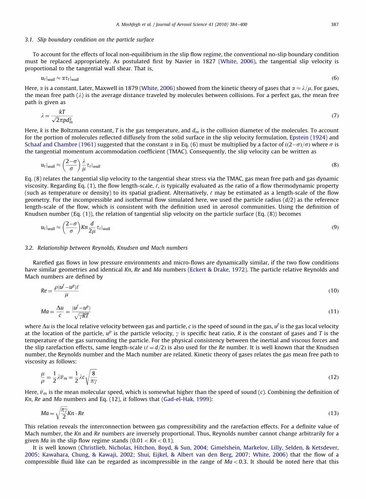
3.1. Slip boundary condition on the particle surface

To account for the effects of local non-equilibrium in the slip flow regime, the conventional no-slip boundary conditionmust be replaced appropriately. As postulated first by Navier in 1827 (White, 2006), the tangential slip velocity isproportional to the tangential wall shear. That is,

ut jwall � attjwall ð6Þ

Here, a is a constant. Later, Maxwell in 1879 (White, 2006) showed from the kinetic theory of gases that a� l=m. For gases,the mean free path (l) is the average distance traveled by molecules between collisions. For a perfect gas, the mean freepath is given as

l¼kTffiffiffi

2p

ppd2m

ð7Þ

Here, k is the Boltzmann constant, T is the gas temperature, and dm is the collision diameter of the molecules. To accountfor the portion of molecules reflected diffusely from the solid surface in the slip velocity formulation, Epstein (1924) andSchaaf and Chambre (1961) suggested that the constant a in Eq. (6) must be multiplied by a factor of ðð2�sÞ=sÞ where s isthe tangential momentum accommodation coefficient (TMAC). Consequently, the slip velocity can be written as

ut jwall �2�ss

� �lm ttjwall ð8Þ

Eq. (8) relates the tangential slip velocity to the tangential shear stress via the TMAC, gas mean free path and gas dynamicviscosity. Regarding Eq. (1), the flow length-scale, ‘, is typically evaluated as the ratio of a flow thermodynamic property(such as temperature or density) to its spatial gradient. Alternatively, ‘ may be estimated as a length-scale of the flowgeometry. For the incompressible and isothermal flow simulated here, we used the particle radius (d/2) as the referencelength-scale of the flow, which is consistent with the definition used in aerosol communities. Using the definition ofKnudsen number (Eq. (1)), the relation of tangential slip velocity on the particle surface (Eq. (8)) becomes

ut jwall �2�ss

� �Kn

d

2mttjwall ð9Þ

3.2. Relationship between Reynolds, Knudsen and Mach numbers

Rarefied gas flows in low pressure environments and micro-flows are dynamically similar, if the two flow conditionshave similar geometries and identical Kn, Re and Ma numbers (Eckert & Drake, 1972). The particle relative Reynolds andMach numbers are defined by

Re¼rjuf�upj‘

mð10Þ

Ma¼Du

c¼juf�upjffiffiffiffiffiffiffiffiffi

gRTp ð11Þ

where Du is the local relative velocity between gas and particle, c is the speed of sound in the gas, uf is the gas local velocityat the location of the particle, up is the particle velocity, g is specific heat ratio, R is the constant of gases and T is thetemperature of the gas surrounding the particle. For the physical consistency between the inertial and viscous forces andthe slip rarefaction effects, same length-scale ð‘¼ d=2Þ is also used for the Re number. It is well known that the Knudsennumber, the Reynolds number and the Mach number are related. Kinetic theory of gases relates the gas mean free path toviscosity as follows:

mr¼

1

2lvm ¼

1

2lc

ffiffiffiffiffiffi8

pg

sð12Þ

Here, vm is the mean molecular speed, which is somewhat higher than the speed of sound (c). Combining the definition ofKn, Re and Ma numbers and Eq. (12), it follows that (Gad-el-Hak, 1999):

Ma¼

ffiffiffiffiffiffipg2

rKn � Re ð13Þ

This relation reveals the interconnection between gas compressibility and the rarefaction effects. For a definite value ofMach number, the Kn and Re numbers are inversely proportional. Thus, Reynolds number cannot change arbitrarily for agiven Ma in the slip flow regime stands (0.01oKno0.1).

It is well known (Christlieb, Nicholas, Hitchon, Boyd, & Sun, 2004; Gimelshein, Markelov, Lilly, Selden, & Ketsdever,2005; Kawahara, Chung, & Kawaji, 2002; Shui, Eijkel, & Albert van den Berg, 2007; White, 2006) that the flow of acompressible fluid like can be regarded as incompressible in the range of Mao0.3. It should be noted here that this

ARTICLE IN PRESS


criterion is necessary but not sufficient. There are flow conditions for which Mach number is smaller than 0.3, but thecompressibility effects may be a prominent feature of the physics of the flow. For example, wall heating or cooling maycause the density to change significantly, and the compressibility may become important even at low Mach numbers.Another example is for flows in micro-devices (especially the confined microflows), where the pressure may changesharply due to viscous effects (Gad-el-Hak, 1999).

Here, we are concerned with an isothermal and unconfined incompressible slip flow past small spheres. The cases withMao0.3 ware studied and the variations of drag force with Kn and Re were analyzed. The low Mach number flows areassumed to be incompressible.

4. Numerical simulation

4.1. Computational domain and imposed boundary conditions

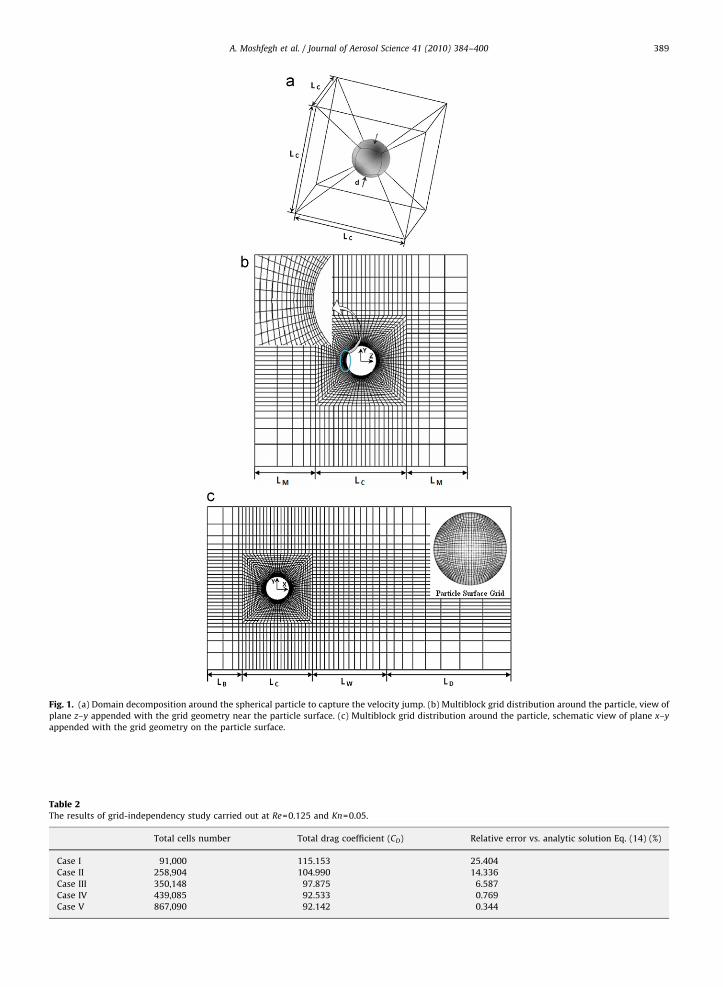
GAMBIT version 2.0.0, the companion package of commercial software FLUENTTM, was used to build the modelgeometry and the computational grids. A multiblock structured and body-fitted grid was considered for analyzing the flowover a single spherical particle with the diameter of d. The layout of multiblock domain decomposition and tri-dimensionalgrid distribution are illustrated in Fig. 1. Such topology of computational domain was used earlier by Jones and Clarke(2003) and Lee (2000), respectively, for the turbulent and laminar unsteady flows over the sphere. Domain decompositionaround the particle to capture the velocity jump at the gas–solid interface is shown in Fig. 1(a). The view of plane z–y andthe grid geometry adjacent to the particle surface are depicted in Fig. 1(b). The view of plane x–y and the grid geometry onthe particle surface are also shown in Fig. 1(c).

The near-wall velocity gradient in the slip flow regime is considerably less than what is appeared in the case where theno-slip boundary condition imposed. Therefore, it was not necessary to consider a spherical domain close to the particlesurface to resolve the boundary layer with a high-resolution grid. Grid elements in the cubic block surrounding the particleare all hexahedral with linear stretching while the other blocks are filled with rectangular elements with exponentialstretching. The geometric lengths of the computational domain depicted in Fig. 1 were selected regarding the flowgeometry at low Reynolds number regimes. In the z–y view, the sides of the cube surrounding the particle (LC) and themarginal lengths (LM) were, respectively, set to 3d and 2d. These values yield a side length of 7d for the square cross-sectionof the computational domain. Along the line of the work presented by Jones and Clarke (2003) on turbulent flow over anunconfined sphere, we found the side length far enough to remove the outer boundary effects on the incompressible andsteady flow simulated here.

To minimize the outflow effects on the flow, the outflow was placed 10d farther from the particle center, 1d more thanwhat was taken for the turbulent flow study by Jones and Clarke (2003). To ensure that the sphere does not affect theuniform inflow, we used the upstream distance from the particle center of 3d following the results of grid-independencystudy reported in the Lee (2000). Therefore, in the x–y view, the beginning length (LB), the wake length (LW) and thedownstream length (LD) are, respectively, equal to 1.5d, 3.5d and 5d. Five different grid resolutions (Cases I, II, III, IV and V)were picked to perform the grid-independency study by measuring the total drag force on the particle at Re=0.125 andKn=0.05. The results are given in the Table 2. From the values given in the relative error column, it could be concluded thatthe Case IV is the best choice among others to achieve a grid-independent solution.

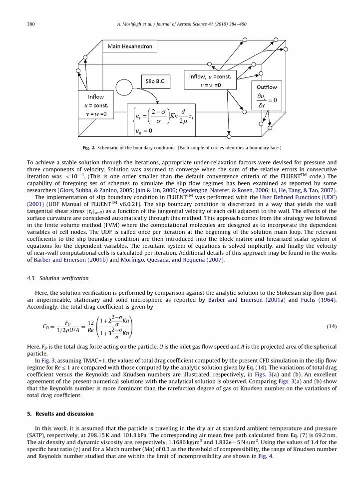
Boundary conditions considered to solve the flow are introduced in Fig. 2. For a fine particle traveling in the gas flow,the gas approaches the particle with a roughly uniform velocity distribution. The left, upper, lower, back and front faces ofthe computational domain were all treated as velocity inlet with a given velocity component along the x-direction. Thedistance from the particle center to the outflow captures successfully the flow steady wake past the particle and alsoensures the assumption of zero gradients of flow variables across the outlet boundary. On the particle surface, the slip(velocity jump) boundary conditions were imposed (in three dimensions).

4.2. Numerical solution

The commercial CFD software FLUENTTM v6.0.12 was adopted to solve the Navier–Stokes equations using the finite-volume method (FVM). The pressure-based segregated algorithm was employed to discretize the 3D, incompressible,steady, laminar and Navier–Stokes equations (Eqs. (2)–(5)). Modified quadratic upstream interpolation for convectivekinematics (QUICK) scheme, which can be implemented on the multidimensional, non-uniform and unstructured grids(Davis, Noye, & Fletcher, 1984; Freitas, Street, Findikakis, & Koseff, 1985; Ji and Wang, 1990; Ji and Wang, 1991; Leonard,1979; Leonard and Mokhtari, 1990), was selected to discretize the convective and diffusive fluxes in the momentumequations. Pressure-velocity coupling was treated by the SIMPLE-consistent (SIMPLEC) algorithm on a colocated grid. Asecond-order pressure interpolation method was also used to calculate the pressure at cell faces from the neighboringnodes. Gradient reconstruction was performed by Green–Gauss node-based formulation (FLUENTTM v6.0.21 User’s Guide).

FLUENTTM solves the linearized scalar system of equations for the dependent variables in each cell using a point implicit(Gauss–Seidel) block matrix linear equation solver in conjunction with an algebraic multi-grid (AMG) method. Flexiblemultigrid cycle was chosen for the three momentum equations, while the V-cycle was considered for continuity equation.

ARTICLE IN PRESS

Fig. 1. (a) Domain decomposition around the spherical particle to capture the velocity jump. (b) Multiblock grid distribution around the particle, view of

plane z–y appended with the grid geometry near the particle surface. (c) Multiblock grid distribution around the particle, schematic view of plane x–y

appended with the grid geometry on the particle surface.

Table 2The results of grid-independency study carried out at Re=0.125 and Kn=0.05.

Total cells number Total drag coefficient (CD) Relative error vs. analytic solution Eq. (14) (%)

Case I 91,000 115.153 25.404

Case II 258,904 104.990 14.336

Case III 350,148 97.875 6.587

Case IV 439,085 92.533 0.769

Case V 867,090 92.142 0.344


ARTICLE IN PRESS

Fig. 2. Schematic of the boundary conditions. (Each couple of circles identifies a boundary face.)


To achieve a stable solution through the iterations, appropriate under-relaxation factors were devised for pressure andthree components of velocity. Solution was assumed to converge when the sum of the relative errors in consecutiveiteration was o10�4. (This is one order smaller than the default convergence criteria of the FLUENTTM code.) Thecapability of foregoing set of schemes to simulate the slip flow regimes has been examined as reported by someresearchers (Giors, Subba, & Zanino, 2005; Jain & Lin, 2006; Ogedengbe, Naterer, & Rosen, 2006; Li, He, Tang, & Tao, 2007).

The implementation of slip boundary condition in FLUENTTM was performed with the User Defined Functions (UDF)(2001) (UDF Manual of FLUENTTM v6.0.21). The slip boundary condition is discretized in a way that yields the walltangential shear stress ðttjwallÞ as a function of the tangential velocity of each cell adjacent to the wall. The effects of thesurface curvature are considered automatically through this method. This approach comes from the strategy we followedin the finite volume method (FVM) where the computational molecules are designed as to incorporate the dependentvariables of cell nodes. The UDF is called once per iteration at the beginning of the solution main loop. The relevantcoefficients to the slip boundary condition are then introduced into the block matrix and linearized scalar system ofequations for the dependent variables. The resultant system of equations is solved implicitly, and finally the velocityof near-wall computational cells is calculated per iteration. Additional details of this approach may be found in the worksof Barber and Emerson (2001b) and Morınigo, Quesada, and Requena (2007).

4.3. Solution verification

Here, the solution verification is performed by comparison against the analytic solution to the Stokesian slip flow pastan impermeable, stationary and solid microsphere as reported by Barber and Emerson (2001a) and Fuchs (1964).Accordingly, the total drag coefficient is given by

CD ¼FD

1=2rU2A¼

12

Re

1þ22�ss Kn

1þ32�ss Kn

0B@

1CA ð14Þ

Here, FD is the total drag force acting on the particle, U is the inlet gas flow speed and A is the projected area of the sphericalparticle.

In Fig. 3, assuming TMAC=1, the values of total drag coefficient computed by the present CFD simulation in the slip flowregime for Rer1 are compared with those computed by the analytic solution given by Eq. (14). The variations of total dragcoefficient versus the Reynolds and Knudsen numbers are illustrated, respectively, in Figs. 3(a) and (b). An excellentagreement of the present numerical solutions with the analytical solution is observed. Comparing Figs. 3(a) and (b) showthat the Reynolds number is more dominant than the rarefaction degree of gas or Knudsen number on the variations oftotal drag coefficient.

5. Results and discussion

In this work, it is assumed that the particle is traveling in the dry air at standard ambient temperature and pressure(SATP), respectively, at 298.15 K and 101.3 kPa. The corresponding air mean free path calculated from Eq. (7) is 69.2 nm.The air density and dynamic viscosity are, respectively, 1.1686 kg/m3 and 1.832e�5 N s/m2. Using the values of 1.4 for thespecific heat ratio (g) and for a Mach number (Ma) of 0.3 as the threshold of compressibility, the range of Knudsen numberand Reynolds number studied that are within the limit of incompressibility are shown in Fig. 4.

ARTICLE IN PRESS

Fig. 3. Comparison of total drag coefficient calculated by analytic solution with that computed by present simulation at s=1: (a) total drag coefficient vs.

the relative Reynolds number and (b) total drag coefficient vs. the Knudsen number.


In theory, TMAC, which accounts for the average tangential momentum exchange across the gas–solid interface, can beassigned by the values ranging from the zero (specular reflection) up to the unity (diffuse reflection). Thomas and Lord(1974) and Arkilic, Schmidt, and Breuer (1997) empirically determined the TMAC values of some materials in the range of0.2–1.0. This parameter depends on both gas and solid materials, and surface finish of the wall (Arkilic et al., 1997).Accordingly, silicon micro-machined components exhibit the TMAC values ranging from the 0.8 to 1.0 (Arkilic et al., 1997).Here, we assumed a value of unity for the TMAC to study the slip correction factor and drag coefficient for most commonmaterials. Computer simulations are performed for five values of Knudsen number distributed uniformly within the slipflow range (0.01oKno0.1), and 83 non-uniform distributed values of Reynolds number selected from the Stokes regimeup to the threshold of compressibility shown in Fig. 4.

5.1. Slip correction factor in Stokesian slip regimes

An important assumption in the Stokes drag force is that the relative velocity of the gas at the surface of the particle iszero. This assumption is not accurate for small particles whose diameters are of the order of or smaller than the mean freepath of the surrounding gas. These particles settle faster than what is predicted by the Stokes law, because of the ‘‘slip’’ atthe surface of the particle (Hinds, 1998). As noted before, Cunningham-based slip corrections were developed for the

ARTICLE IN PRESS

Fig. 4. Incompressible cases (scatter data points) studied in the paper involving 83 data points including eight uniformly distributed points in Stokes’

regime at each Kn number.

Fig. 5. Slip correction factor calculated from Eq. (15) using the numerical results.


Stokes flow regime. Hence in the present work, the new slip correction factor is proposed in the range 0oReo1 or theStokes regime.

In gas–solid two-phase flows, dynamic characteristics of the particle, such as terminal velocity, relaxation time, Stokesnumber and etc., are directly proportional to the Cunningham–Stokes slip correction factor. To account for the slip effectson the particle drag force in the rarefied regimes, Cunningham slip correction factor (Cc) is defined as a function of Knudsennumber in the Stokesian flow regime. That is,

Cc ¼3pmUd

Fslip¼ fcnðKnÞ41:0 for Re51 ð15Þ

where the numerator denotes the analytical drag force experienced by the particle in the continuum Stokes ðRe51Þ flow,and Fslip is the drag force in the slip flow regime. This relation assumes that the particle drag force ðFslipÞ is decreased by therarefaction effects as a function of Knudsen number.

In this section, it will be shown that the slip correction factor evaluated by Stokes’ drag formula is accurate only for Re

numbers very close to zero where the inertial forces are negligible. To better recognize the philosophy of the slip correctionfactor, we separate the slip dynamic effects on the particle to two exactly opposite phenomena. One is the flow dynamiceffect which pertains to the nature of continuum regime that we call it ‘‘continuum effects’’, and the other is all differencesexist between the continuum and slip regimes which can be referred as ‘‘pure rarefaction effects’’. The latter effectincorporates the flow rarefaction effects which deviate the flow behaviors from what is observed in the non-slip

ARTICLE IN PRESS


continuum regime. Since this factor (Eq. (15)) has been defined as a function of Kn number, it should represent the ‘‘purerarefaction effects’’. But it is shown that this conventional definition of slip correction not only represents the ‘‘purerarefaction effects’’ but also contains some inertial effects coming from the ‘‘continuum effects’’. The slip correction factor(Eq. (15)) in comparison to Cunningham-based corrections (Table 1) is illustrated in Fig. 5.

A visual detection in the diagrammed behavior reveals that the slip correction factor calculated using Eq. (15) is lessthan unity in some areas. It is a rudimentary fact that rarefied regimes always reduce the particle drag force. Disability ofStokes’ drag formula to account for all inertia effects of the flow combines with the ‘‘pure rarefaction effects’’ representedby Eq. (15), and then ignores the fluid slip in the non-physical territory identified in Fig. 5. By a simple extrapolation on thisfigure, it is evident that for very low Reynolds numbers (too close to the zero) the computed slip correction shows acompletely physical behavior ðCc Z1:0Þ. The increment of Reynolds number mitigates the accuracy of Stokes’ formula topredict the real drag force (or real ‘‘continuum effects’’). This brings about some artificial (or unreal) ‘‘pure rarefactioneffect’’ posing itself through the term ð3pmUdÞ and Eq. (15), and hence some parts of these graphs become subunit.

To ensure the speculated root of this behavior, we use a more rational definition of slip correction factor, which can befound in the literatures (Rader, 1990), as follows:

Slip correction factor ðSCFÞ ¼Fcont:

FSlipð16Þ

where Fcont: is the particle drag force in the continuum no-slip regime. The experimental data are more realistic andsensible than the numerical ones to evaluate Fcont:. Therefore, we use the drag formula derived by Oseen (1910) (modifiedfor Reynolds number defined based on the particle radius) as given below

Fcont: ¼12

Re1þ

3

8Re

� �1

2rU2A

� �ð17Þ

Fig. 6 shows the numerical slip correction factors evaluated using Eqs. (16) and (17) in the Stokesian regime. As wasnoted before, there is no available experimental data for Fslip in this range. Here, the numerical simulation data for the dragforce in the slip flow regime are used. Fig. 6 shows that the resultant slip correction factor is always greater than unity andincreases roughly linearly with Kn. It is also seen that the slip corrections varies significantly depending on Reynoldsnumber. The observed dependence on Re, suggests that the correlation for slip correction should include variations of Re.As was recognized by some researchers (Kavehpour, Faghri, & Asako, 1997; White, 2006; Zuppardi, Paterna, & Rega, 2007),the fluid inertia or Reynolds number has an important role to mitigate and/or intensify the rarefaction effects in the slipflow regimes. Fig. 6 clearly shows that higher values of Re lead to higher rarefaction effects and consequently higher fluidslip on the particle surface that yields higher values of SCF.

A comparison between the Cunningham-based correlations (Table 1) and the slip correction factor computed throughthe present simulation using Eqs. (16) and (17) is also carried out in Fig. 6. The computed slip correction factor is under-predicted by the Cunningham-based corrections (Table 1). These correlations were proposed for very close Reynoldsnumbers to zero (using the Stokes’ formula), and they neglect the Re prominence on the slip correction, so this brings aboutconsiderable under-prediction by Cunningham-based correlations in the range 05Reo1. As one closes to the Re=0,computed SCF approaches the corrections reported in Table 1 that proves the accuracy of the computed data via Eq. (16) atthe limiting case of creeping (very low Reynolds number) flows. The difference percentage of computed SCF from the ones

Fig. 6. Comparison of Cunningham-based correlations (Table 1) and computed slip correction (Eq. (16)).

ARTICLE IN PRESS

4.6

5.6

6.6

7.6

8.6

Re = 0.25

8.5

9.5

10.5

11.5

12.5

Re = 0.37512.0

13.0

14.0

15.0

16.0

Re = 0.5

15.5

16.5

17.5

18.5

Re = 0.625

Cc

off %

: (Ta

b. 1

) & H

inds

18.5

19.5

20.5

21.5

Re = 0.75

Cc

off %

: (Ta

b. 1

) & H

inds

21.5

22.5

23.5

24.5

Re = 0.875

Cc

off %

: (Ta

b. 1

) & H

inds

24.0

25.0

26.0

27.0

Re = 1.0

Cc

off %

: (Ta

b. 1

) & H

inds

0.5

1.5

2.5

3.5

4.5

0.01Kn

Cc1Cc2Cc3Cc4Cc5Cc6Cc7Cc8Cc9




Cc

off %

: (Ta

b. 1

) & H

inds

Cc

off %

: (Ta

b. 1

) & H

inds

Cc

off %

: (Ta

b. 1

) & H

inds

Cc

off %

: (Ta

b. 1

) & H

inds

Re = 0.125

0.055 0.1

0.01Kn

0.055 0.1

0.01Kn

0.055 0.1

0.01Kn

0.055 0.1 0.01Kn

0.055 0.1



0.01Kn

0.055 0.1


0.01Kn

0.055 0.1


0.01Kn

0.055 0.1

Fig. 7. The error percentage of SCF given by Eq. (16) and the ones reported in Table 1.


listed in Table 1 is also diagrammed in Fig. 7 at each Reynolds number. According to these diagrams, inaccuracy of SCFs

listed in Table 1 increase as the gas rarefaction effect increases, and finally touches its maximum value (27%) at Re=1.Barber and Emerson (2002b) studied the effects of Kn and Re numbers on the hydrodynamic development length in

circular and parallel plate ducts. Similar to Fig. 6, their results showed that both Reynolds and Knudsen numbers affect theslip flow physical parameters in a similar manner (in some flow cases). The increment of both numbers (Kn, Re) intensifiesthe gas slip as recorded in Fig. 6. Zuppardi et al. (2007) quantified the effects of rarefaction in high velocity slip flowregimes, and reported that both slip velocity and temperature jump are increased when the free stream velocity (or theflow Reynolds number) increases.

Regarding such behaviors, the Cunningham-based slip corrections (Table 1) do not seem to be appropriate to describecompletely the rarefaction effects only through the Knudsen number. One main goal in this study is to modify the slipcorrection factor based on the Cunningham’s mathematical definition (Fcont: divided by Fslip). In particular, we plan to

ARTICLE IN PRESS

Table 3Coefficients and statistics of curve-fitted correlation (Eq. (18)).

Coefficient Mean value Uncertainty (SD) RS=0.998

A 0.23994 0.193E�1 ARS=0.998

B 2.0024 0.980E�3 SDF=0.257E�02

C 0.97832 0.397E�2 AAR=0.190E�02

Fig. 8. The 3D fitted curve for new proposed slip correction factor (SCF) at Eq. (18).


incorporate the dependence of slip correction on the Reynolds number in the correlation. Therefore, a correction as afunction of both relative Re and Kn numbers has to be prepared. Curve-fit statistics were analyzed quantitatively and it wasfound that the original form of Cunningham correction (Eq. (1)) is just appropriate to correlate the Kn variations in the slipregime when the Re is considered to be fixed. The original form can be multiplied by an additional term to introduce the Re

into the correction. Several additional functions of Reynolds number were tested and it was recognized that the basicproposed form of Cunningham correction (Eq. (1)) is not the best choice for 3D curve-fitting process involving both Kn andRe numbers. Exponential curve fitting (Eq. (1)) is commonly used when the rate of variations accelerates suddenly, so theCunningham-based correlations are appropriate to correlate the rarefaction effects over a wide range of Knudsen numbers,but this is not the case in the slip flow regime. Moreover, if we could find an appropriate additional expression as a functionof Re, the final slip correction would be too large in terms, and could not be utilized easily by the users during the particletracking procedure. Here, we propose a novel and concise expression (Eq. (18)) which was the best among the 480 tested3D functions.

SCF ¼ AðReÞþBðKnÞþC for 0oReo1 and 0:01oKno0:1 ð18Þ

The calculated coefficients and the curve fit statistics (Refer to the Appendix A.) are given in the Table 3. The meanvalues of computed coefficients, standard deviation (SD) or uncertainty of fitted coefficients, RS, ARS, standard deviation ofthe fitting (SDF) and average absolute residual (AAR) have been also reported.

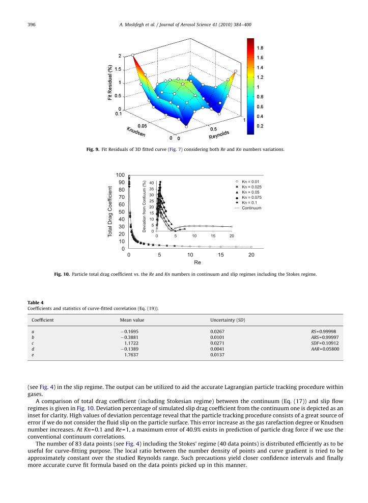
The 3D fitted curve on the computed slip correction factors based on Eq. (16) is illustrated in Fig. 8. Scatter data pointsplaced on the solid lines represent the computed data, and the 3D curve denotes the fitted (predicted) data by Eq. (18). Thefit residual at each data point is also demonstrated vs. the Knudsen and Reynolds numbers in Fig. 9. Maximum errorthrough the curve-fitting process amounts to o1.9% that shows an acceptable fit.

5.2. Moderate Reynolds slip flow

No experiment and numerical studies among the ones which were cited (see Literature Review section) consider theinfluence of Re through their slip flow investigation. Here, similar to what was carried out in the continuum flow regime(Clift, Grace, & Weber, 1978;; Hinds, 1982; Oseen, 1910; White, 2006), and in order to correlate the particle drag coefficientwith flow dimensionless parameters, we intend to propose a two-variable correlation over a moderate range of flow speeds

ARTICLE IN PRESS

1009080706050403020100

Tota

l Dra

g C

oeffi

cien

t

0

0

5

5

10

10

15

15

20

20

Re

4035302520151050D

evia

tion

from

Con

tiuum

(%) Kn = 0.01

Kn = 0.025Kn = 0.05Kn = 0.075Kn = 0.1Continuum

Fig. 10. Particle total drag coefficient vs. the Re and Kn numbers in continuum and slip regimes including the Stokes regime.

Fig. 9. Fit Residuals of 3D fitted curve (Fig. 7) considering both Re and Kn numbers variations.

Table 4Coefficients and statistics of curve-fitted correlation (Eq. (19)).

Coefficient Mean value Uncertainty (SD)

a �0.1695 0.0267 RS=0.99998

b �0.3881 0.0101 ARS=0.99997

c 1.1722 0.0271 SDF=0.10912

d �0.1389 0.0041 AAR=0.05800

e 1.7637 0.0137


(see Fig. 4) in the slip regime. The output can be utilized to aid the accurate Lagrangian particle tracking procedure withingases.

A comparison of total drag coefficient (including Stokesian regime) between the continuum (Eq. (17)) and slip flowregimes is given in Fig. 10. Deviation percentage of simulated slip drag coefficient from the continuum one is depicted as aninset for clarity. High values of deviation percentage reveal that the particle tracking procedure consists of a great source oferror if we do not consider the fluid slip on the particle surface. This error increase as the gas rarefaction degree or Knudsennumber increases. At Kn=0.1 and Re=1, a maximum error of 40.9% exists in prediction of particle drag force if we use theconventional continuum correlations.

The number of 83 data points (see Fig. 4) including the Stokes’ regime (40 data points) is distributed efficiently as to beuseful for curve-fitting purpose. The local ratio between the number density of points and curve gradient is tried to beapproximately constant over the studied Reynolds range. Such precautions yield closer confidence intervals and finallymore accurate curve fit formula based on the data points picked up in this manner.

ARTICLE IN PRESS

Fig. 11. The 3D fitted curve of proposed total drag coefficient for non-Stokesian and incompressible slip flow including the 83 data points.


After searching among a library of 37 860 functions including linear, nonlinear, polynomials, rational and logarithmicequations and some combinations of them, the following correlation was found to be economic in size and order ofaccuracy.

lnðCDÞ ¼ aþb lnðReÞþc=ffiffiffiffiffiffiRepþd=Reþe expð�KnÞ for

Incompressible

Slip : 0:01oKno0:1

( )gas flows ð19Þ

This correlation covers the values of Re and Kn numbers which yield the Stokesian, incompressible and slip gas flows. Thecorresponding curve fit statistics are tabulated in the Table 4.

Computed data points with the 3D fitted curve using Eq. (19) are illustrated in Fig. 11. A reasonable covering of scatterdata points by the proposed formula is discernable.

6. Conclusions

In the present work, the incompressible slip flow regime past an unconfined, stationary, impermeable, solid andspherical aerosol particle was simulated. Gas slip on the particle surface was treated numerically by the imposition of slipboundary condition. The simulations were implemented over a range of Reynolds numbers from the Stokesian regime upto threshold of compressibility where the flow stays roughly steady. Novel formulations were proposed to correlate the slipcorrection factor and particle total drag coefficient against both Knudsen and Reynolds numbers. Based on the presentedresults, the following conclusions are drawn:

(1)
Slip correction factor in conjunction with Stokes drag formula is accurate only for Re numbers very close to zero wherethe inertial forces of the flow approaches zero. But for slightly larger Re numbers ð05Reo1Þ, the simple Stokes’ dragusage in the slip correction factor leads to subunit values of Cc. Disability of Stokes’ drag formula to account for allinertia effects of the flow combines with the ‘‘pure rarefaction effects’’ represented by Eq. (15), and then ignores thefluid slip on the particle surface. The increment of Reynolds number mitigates the accuracy of Stokes’ formula topredict the real drag force (or real ‘‘continuum effects’’). This brings about some artificial (or unreal) ‘‘pure rarefactioneffect’’ which shows itself through the term ð3pmUdÞ and Eq. (15), and hence for the Re numbers far from zero thephysical condition Cc Z1:0 does not meet. A more rational definition of slip correction factor, which replaces theStokes’ drag with experimental drag force in the continuum regime, overcomes the problem completely.
(2)
A prominent difference between the slip corrections at different Reynolds numbers is readily discernable. Thisdifference necessitates the incorporation of Re number into the correlations (such as slip correction factor and dragcoefficient) which parameterize the drag force in the slip regime. The Reynolds number has a profound effect on theslip correction factor similar to the Knudsen number. The computed slip correction factors are all under-predicted bythe Cunningham-based corrections (Table 1) in the range 05Reo 1. These correlations were proposed for very closeReynolds numbers to zero, and they neglect the Re number prominence on the slip correction, so this brings aboutconsiderable under-prediction by Cunningham-based correlations in this range of Re number. Deviation of SCFs listedin Table 1 from the presented data incorporating the inertia effects (Re number) increases as the gas rarefaction effectis intensified, and finally reaches its maximum value (27%) at Re=1. Higher values of Re lead to higher rarefactioneffects and consequently higher gas slip on the particle surface. In the other word, both Re and Kn numbers affect the

ARTICLE IN PRESS


slip flow parameters such as slip correction factor and drag coefficient in a same manner. The increment of thesenumbers (Kn, Re) intensifies the gas slip on the particle.

(3)
Exponential behavior of the flow rarefaction effects that appears in a wide range of Knudsen numbers does not hold inthe slip flow regime. Therefore, the definition of the Cunningham-based correlations is not appropriate to be used forthe slip correction factor (and curve-fitting purposes) in the slip regime especially when the Reynolds number has beenincorporated into the correction. A novel slip correction factor with a maximum error of 1.9% was proposed.
(4)
Proposed correlation for the total drag coefficient of the spherical particle (in the range 0.01oKno0.1 and0.125oReo20) enhances the accuracy of particle drag force prediction in gas–solid two-phase flow simulations up tothe 40.9% at the worst condition which occurs in most rarefied slip regime (at Kn=0.1 and Re=1).
Appendix A. Curve fitting theory

The fitting process requires a model that relates the computed data to the predictor data with one or more coefficients througha special formula. Due to the nonlinear behavior of drag coefficient acting by the slip flow regime on a suspending sphericalparticle, similar to what was recognized in the continuum regime, we use the nonlinear least squares model (Bevington, 1969;Press, Teukolsky, Vetterling, & Flannery, 2002; Press et al., 1988) to propose the correlations herein. A nonlinear model is definedas an equation that is nonlinear in the coefficients. In matrix form, nonlinear models are given by this formula

z¼ f ðX;wÞþe ðA:1Þ

Here, z is a n-by-1 vector including the n numbers of computed data, f is the correlated formula as a function of X and w, where Xis an n-by-m design matrix for the model, w is a m-by-1 vector of coefficients and e is a n-by-1 vector of errors. Nonlinear modelsare more difficult to fit than the linear ones because the coefficients cannot be estimated using simple matrix techniques. In anonlinear equation, the partial derivative with respect to one coefficient will include one or more of other coefficients, making asingle step matrix solution for the individual coefficients impossible. Therefore, an iterative approach is required. To estimate thecoefficients, the nonlinear least squares method minimizes the sum of squared residuals. Assuming that n data points are availableto be fitted, the residual (Rj) of the jth data point is defined as the difference between the computed value (zj) and the estimatedone ðzjÞ as given below

Rj ¼ zj�z j ðA:2Þ

The sum of squared residuals (S) is therefore expressed by

S¼Xn

k ¼ 1

R2j ¼

Xn

k ¼ 1

ðzj�z jÞ2

ðA:3Þ

A residual is thus the vertical z-distance between the fitted surface and a data point in 3D curve-fitting process. Least-squaresminimization assumes that x and y are accurately determined, and that an error exists only in the dependent variable z. In thiscase, however, it is not possible to express the partial derivatives as a function of only the x or y. It is also assumed that each pointhas the same weight or standard deviation, meaning that each ones are weighted equally in computing the sum of squaredresiduals. There are a variety of methods to converge to the minimum least-squares, that the Levenburg–Marquardt algorithm(Bevington, 1969; Press et al., 1988) is adopted here. There were no prominent outliers to be excluded from the original computeddata set, and consequently, the robust fitting process was not enabled. Convergence tolerance is also considered equal to 1E�6.

A.1. Fit goodness criteria

To evaluate the goodness of curve-fitted formula, there are some parameters describing the quality of fitting process(Chambers, Cleveland, Kleiner, & Tukey, 1983; Cleveland, 1979; Cleveland & Devlin, 1988; Goodall, Fox, & Long, 1990;Hutcheson, 1995; Press, Teukolsky, Vetterling, & Flannery, 1993). Rather than the residuals, we define several additionalstatistic parameters as follow

Sum of squares due to error ðSSEÞ ¼Xn

k ¼ 1

wkðzk�zkÞ2

ðA:4Þ

where wk is the local influence weight factor of kth data point on the fitted curve. SSE denotes the total deviation ofestimated values from the computed ones. Closer value to the zero indicates closer estimated data points to the computedones, and consequently yields a better fit.

Sum of squares of regression ðSSRÞ ¼Xn

k ¼ 1

wkðz�zkÞ2

ðA:5Þ

Sum of squares about mean ðSSMÞ ¼Xn

k ¼ 1

wkðzk�zÞ2 ðA:6Þ

ARTICLE IN PRESS


where z is the mean value of computed data points, and

SSR¼ SSM�SSE ðA:7Þ

R-square ðRSÞ ¼SSR

SSM¼ 1�

SSE

SSMðA:8Þ

The statistics RS measures the degree of fit success in explaining the variation of data. R-square can take on any valuebetween 0 and 1 that a value closer to 1 gives a better fit. Sometimes, increasing the number of data points, which resultsin a closer value of R-square to unity, does not yield a better fit. To ensure the goodness of the fitted curve, adjustedR-square is defined as

Adjusted R-square ðARSÞ ¼ 1�SSEðn�1Þ

SSMðvÞðA:9Þ

Adjusted R-square (ARS) adjusts the R-square statistics based upon the residuals degree of freedom (v). The parameter v isequal to the number of data points (n) minus the number of fitted coefficients (m) which appear in the curve-fittedformula. The parameter v indicates the number of independent data points that are required to calculate the sum ofsquares. ARS is generally the best indicator of the fit goodness when additional unknown coefficients are added to theformula. It is clear that a closer value of ARS to the unity denotes a better fit. In this paper, these parameters are employedto examine the quality of our proposed correlations for both slip correction factor and total drag coefficient.

Confidence bound defines the lower and upper limits of a spatial interval involving the fitted curve, and shows how thefitted curve is uncertain about a newcomer data point which does not exist in the original computed data set. The boundsare defined with a level of certainty that is specified here equal to 95%. This level indicates that you have a 95% chance thata newcomer data point, which has not been simulated by the present computation, is actually contained within the lowerand upper limits of confidence bound. The confidence bounds for the fitted coefficients are given by

C¼ b7t0ffiffiffiffiGp

ðA:10Þ

G¼ ðXT XÞ�1S2 ðA:11Þ

where C includes the confidence bounds for each coefficient, b are the coefficients of the curve-fitted formula, t0 is theinverse of Student’s T cumulative distribution function, XT is the transpose of X and G is a vector of the diagonal elementsfrom the covariance matrix of the estimated coefficients. To calculate the confidence bounds of estimated data points, thevector b in Eq. (10) should be replaced by z.

References

Allen, M. D., & Raabe, O. G. (1982). Re-evaluation of Millikan’s oil drop data for the motion of small particles in air. Journal of Aerosol Science, 13, 537.Allen, M. D., & Raabe, O. G. (1985). Slip correction measurements of spherical solid aerosol particles in an improved Millikan apparatus. Journal of Aerosol

Science and Technology, 4, 269.Arkilic, E. B., Schmidt, M. A., & Breuer, K. S. (1997). TMAC measurement in silicon micromachined channels. Rarefied gas dynamics, Vol. 20. Beijing: Beijing

University Press.Barber, R. W., & Emerson, D. R. (2001a). Analytic solution of low Reynolds number slip flow past a sphere. Centre for Microfluidics, Department of

Computational Science and Engineering, CLRC Daresbury Laboratory, Daresbury, Warrington, WA4 4AD.Barber, R. W., & Emerson, D. R. (2001b). Numerical simulation of low Reynolds number slip flow past a confined microsphere. Technical report DL-TR-01-001,

Centre for Microfluidics, Department of Computational Science and Engineering, CLRC Daresbury Laboratory, Daresbury, Warrington.Barber, R. W., & Emerson, D. R. (2002a). Numerical simulation of low Reynolds number slip flow past a confined microsphere. In 23rd international

symposium on rarefied gas dynamics (pp. 20–25). Whistler, Canada.Barber, R. W., & Emerson, D. R. (2002b). A numerical study of low Reynolds number slip flow in the hydrodynamic development region of circular and parallel

plate ducts. Centre for Microfluidics, Department of Computational Science and Engineering, CLRC Daresbury Laboratory, Daresbury, Warrington, WA44AD.

Bevington, P. R. (1969). Data reduction and error analysis for the physical sciences. New York: McGraw-Hill.Chambers, J., Cleveland, W. S., Kleiner, B., & Tukey, P. (1983). Graphical methods for data analysis. Belmont, CA: Wadsworth International Group.Chomaz, J. M., Bonneton, P., & Hopfinger, E. J. (1993). The structure of the near wake of a sphere moving horizontally in a stratified fluid. Journal of Fluid

Mechanics, 254, 1–21.Christlieb, A. J., Nicholas, W., Hitchon, G., Boyd, I. D., & Sun, Q. (2004). Kinetic description of flow past a micro-plate. Journal of Computational Physics, 195,

508–527.Cleveland, W. S. (1979). Robust locally weighted regression and smoothing scatterplots. Journal of the American Statistical Association, 74, 829–836.Cleveland, W. S., & Devlin, S. J. (1988). Locally weighted regression: An approach to regression analysis by local fitting. Journal of the American Statistical

Association, 83, 596–610.Clift, R., Grace, J. R., & Weber, M. W. (1978). Bubbles, drops and particles. New York: Academic Press.Constantinescu, G. S., & Squires, K. D. (2000). LES and DES investigations of turbulent flow over a sphere. American Institute of Aeronautics and Astronautics

(AIAA) paper 2000-0540.Crowe, C. T. (Ed.). (2006). Multiphase flow handbook (1st ed). Florida: Taylor & Francis.Cunningham, E. (1910). On the velocity of steady fall of spherical particles through fluid medium. Proceedings of Royal Society (London) A, 83, 357–365.Davies, C. N. (1945). Definite equations for the fluid resistance of spheres. Proceedings of Physics Society, 57, 18.Davis, R. W., Noye, J., & Fletcher, C., (Eds.) (1984). Finite difference methods for fluid flow. Computational techniques and applications (pp. 51–69). Elsevier:

Amsterdam.Dhaniyala, S., Wennberg, P. O., Flagan, R. C., Fahey, D. W., Northway, M. J. Gao, R. S., et al. (2004). Stratospheric aerosol sampling: effect of a blunt-body

housing on inlet sampling characteristics. Journal of Aerosol Science and Technology, 38, 1080–1090.Eckert, E. R.G., & Drake, R. M., Jr. (1972). Analysis of heat & mass transfer (pp. 467–486). New York: McGraw-Hill Inc.Epstein, P. S. (1924). Physics Review, 23, 710–733.

ARTICLE IN PRESS


Fluent, Inc., 2001. Fluent 6.0.12 User’s Guide. Fluent, Inc., Centerra Resource Park, 10 Cavendish Court, Lebanon, NH 03766, USA.Freitas, C. J., Street, R. L., Findikakis, A. N., & Koseff, J. R. (1985). Numerical simulation of three-dimensional flow in a cavity. International Journal of

Numerical Methods in Fluids, 5, 561–575.Fremerey, J. K. (1982). Spinning rotor vacuum gauges. Vacuum, 32, 685–690.Fuchs, N. A. (1964). The mechanics of aerosols. New York: Pergamon Press.Gad-el-Hak, M. (1999). The fluid mechanics of microdevices—the Freeman scholar lecture. Journal of Fluids Engineering, 121, 5–33.Gimelshein, S. F., Markelov, G. N., Lilly, T. C., Selden, N. P., & Ketsdever, A. D. (2005). Experimental and numerical modeling of rarefied gas flows through

orifices and short tubes. In 24th international symposium on rarefied gas dynamics (pp. 437–443).Giors, S., Subba, F., & Zanino, R. (2005). Navier–Stokes modeling of a Gaede pump stage in the viscous and transitional flow regimes using slip-flow

boundary conditions. Journal of Vacuum Science and Technology A, 23(2), 336–346.Goodall, C., Fox, J., & Long, J. S. (1990). A survey of smoothing techniques, modern methods of data analysis (pp. 126–176). Newbury Park, CA: Sage

Publications.Hinds, W. C. (1982). Aerosol technology, properties behavior, and measurement of airborne particles. New York: John Wiley and Sons.Hinds, W. C. (1998). Aerosol technology, properties behavior, and measurement of airborne particles (2nd ed). New York: John Wiley and Sons.Hutcheson, M. C. (1995). Trimmed resistant weighted scatterplot smooth. Master’s thesis, Cornell University, Ithaca, NY.Hutchins, D. K., Harper, M. H., & Felder, R. L. (1995). Journal of Aerosol Science and Technology, 22, 202.Jain, V., & Lin, C. X. (2006). Numerical modeling of three-dimensional compressible gas flow in microchannels. Journal of Micromechanics and

Microengineering, 16, 292–302.Ji, W., & Wang, P. K. (1990). Numerical simulation of three-dimensional unsteady viscous flow past fixed hexagonal ice crystals in the air—preliminary

results. Atmospheric Research, 25, 539–557.Ji, W., & Wang, P. K. (1991). Numerical simulation of three-dimensional unsteady viscous flow past finite cylinders in an unbounded fluid at low

intermediate Reynolds numbers. Theoretical Computer Fluid Dynamics, 3, 43–59.Jones, D. A., & Clarke, D. B. (2003). An evaluation of the FIDAP computational fluid dynamics code for the calculation of hydrodynamic forces on underwater

platforms. Maritime Platforms Division, Platforms Sciences Laboratory, DSTO-TR-1494.Kavehpour, H. P., Faghri, M., & Asako, Y. (1997). Effects of compressibility and rarefaction on gaseous flows in microchannels. Numerical Heat Transfer, Part

A: Applications, 32, 677–696.Kawahara, A., Chung, P. M.-Y., & Kawaji, M. (2002). Investigation of two-phase flow pattern, void fraction and pressure drop in a microchannel.

International Journal of Multiphase Flow, 28, 1411–1435.Kim, J. H., Mulholland, G. W., Kukuck, S. R., & Pui, D. Y.H. (2005). Slip correction measurements of certified PSL nanoparticles using a nanometer

differential mobility analyzer (Nano-DMA) for Knudsen number from 0.5 to 8. Journal of Research of the National Institute of Standards and Technology,110, 31–54.

Knudsen, M., & Weber, S. (1911). Luftwiderstand gegen die langsame. Bewegung kleiner Kugeln. Annals Physics, 36, 981–994.Lee, S. (2000). A numerical study of the unsteady wake behind a sphere in a uniform flow at moderate Reynolds numbers. Journal of Computers & Fluids,

29, 639–667.Leonard, B. P. (1979). Adjusted quadratic upstream algorithms for transient incompressible convection. A collection of technical papers. AIAA

Computational Fluid Dynamics Conference, AIAA Paper 79-1469.Leonard, B. P., & Mokhtari, S. (1990). ULTRA-SHARP nonoscillatory convection schemes for high-speed steady multidimensional flow. NASA Lewis Research

Center, NASA TM 1-2568 (ICOMP-90-12).Li, A., Ahmadi, G., Bayer, R. G., & Gaynes, M. A. (1994). Aerosol particle deposition in an obstructed turbulent duct flow. Journal of Aerosol Science, 25,

91–112.Li, Z., He, Y-L., Tang, G-H., & Tao, W-Q. (2007). Experimental and numerical studies of liquid flow and heat transfer in microtubes. International Journal of

Heat and Mass Transfer, 50, 3447–3460.Liu, H.-C. F., Beskok, A., Gatsonis, N.,& Karniadakis, G. E. (1998). Flow past a microsphere in a pipe: effects of rarefaction (DSC-Vol. 66, pp. 445–452), Micro-

Electro-Mechanical Systems (MEMS). American Society of Mechanical Engineers (ASME).Millikan, R. A. (1910). The isolation of an ion, a precision measurement of its charge, and the correction of Stokes’s law. Science, 32, 436–448.Millikan, R. A. (1923). The general law of fall of a small spherical body through a gas, and its bearing upon the nature of molecular reflection from surfaces.

Physical Review, 22, 1–23.Millikan, R. A. (1963). The electron: its isolation and measurement and the determination of some of its properties (8th ed). Chicago: University of Chicago

Press.Morınigo, J. A., Quesada, J. H., & Requena, F. C. (2007). Slip-model performance for underexpanded micro-scale rocket nozzle flows. In 8th international

symposium on experimental and computational aerothermodynamics of internal flows Lyon. Paper reference: ISAIF8-0026.Ogedengbe, E. O.B., Naterer, G. F., & Rosen, M. A. (2006). Slip-flow irreversibility of dissipative kinetic and internal energy exchange in microchannels.

Journal of Micromechanics and Microengineering, 16, 2167–2176.Oseen, C. W. (1910). Uber die Stokes’sche formel und uber eine verwandte aufgabe in der hydrodynamic. Arkiv for Matematik, Astronomi och Fysik, 6, 29.Peters, T. M., & Leith, D. (2004). Particle deposition in industrial duct bends. Annals of Occupational Hygiene, 1–8.Press, W. H., Teukolsky, S. A., Vetterling, W. T., & Flannery, B. P. (1993). Numerical recipes in C, the art of scientific computing. Cambridge, England:

Cambridge University Press.Press, W. H., Teukolsky, S. A., Vetterling, W. T., & Flannery, B. P. (2002). Numerical recipes in C++; the art of scientific computing (p. 691). Cambridge, UK:

Cambridge University Press.Press, W. H. William, H., et al. (1988). Numerical recipes in C; The art of scientific computing. Cambridge, UK: Cambridge University Press.Rader, D. J. (1990). Momentum slip correction factor for small particles in nine common gases. Journal of Aerosol Science, 21, 161–168.Reich, G. (1982). Spinning rotor viscosity gauge: A transfer standard for the laboratory or an accurate gauge for vacuum process control. Journal of Vacuum

Science and Technology, 20, 1148–1152.Sakamato, H., & Haniu, H. (1990). A study of vortex shedding from spheres in an uniform flow. Journal of Fluid Engineering, 112, 386–392.Schaaf, S. A., & Chambre, P. L. (1961). Flow of rarefied gases. Princeton: Princeton University Press.Shui, L., Eijkel, J. C.T., & Albert van den Berg, S. (2007). Multiphase flow in micro- and nanochannels. Sensors and Actuators, 121, 263–276.Soltani, M., Ahmadi, G., Ounis, H., & McLaughlin, B. (1998). Direct simulation of charged particle deposition in a turbulent flow. International Journal of

Multiphase flow, 24, 77–92.Taneda, S. (1956). Experimental investigations of the wake behind a sphere at low Reynolds numbers. Journal of Physics, Japan, 11(10), 1104–1108.Thomas, L. B., & Lord, R. G. (1974). Comparative measurements of tangential momentum and thermal accommodations on polished and on roughened

steel spheres. In K. Karamcheti (Ed.), Rarefied gas dynamics (8th ed.) (pp. 405–412). New York: Academic Press.UDF (User Defined Functions) Manual, FLUENT 6.0.12, Fluent Inc., November 2001.Wang, X., Gidwani, A., Girshick, S. L., & McMurry, P. H. (2005). Aerodynamic focusing of nanoparticles: II. Numerical simulation of particle motion through

aerodynamic lenses. Journal of Aerosol Science and Technology, 39, 624–636.White, F. M. (2006). Viscous fluid flow. New York: Mc-Graw Hill.Zhang, Z., Kleinstreuer, C., Donohue, J. F., & Kim, C. S. (2005). Comparison of micro- and nano-size particle depositions in a human upper airway model.

Journal of Aerosol Science, 36, 211–233.Zuppardi, G., Paterna, D., & Rega, A. (2007). Quantifying the effects of rarefaction in high velocity, slip-flow regime (published conference proceedings

style). In Rarefied gas dynamics: 25th international symposium, Russia, Novosibirsk, 2007.

A new expression for spherical aerosol drag in slip flow regime

Documents

Transcript of A new expression for spherical aerosol drag in slip flow regime