A model of financial market dynamics with heterogeneousbeliefs and state-dependent confidence

Carl Chiarella (carl.chiarella@uts.edu.au)School of Finance and Economics, University of Technology Sydney, Australia

Roberto Dieci∗(rdieci@rimini.unibo.it)Department of Mathematics for Economic and Social Sciences

University of Bologna, Italy

Laura Gardini (gardini@econ.uniurb.it)Institute of Economics, University of Urbino, Italy

Lucia Sbragia (l.sbragia@uniurb.it)Institute of Economics, University of Urbino, Italy

Abstract

In a simple model of financial market dynamics, we allow the price of a risky securityto be set by a market maker depending on the excess demand of heterogeneous interact-ing traders, fundamentalists and chartists, who place their orders based upon differentexpectations schemes about future prices: while chartists rely on standard trend-basedrules, fundamentalists are assumed to know the economic environment and to form theirbeliefs accordingly. As price moves away from the long-run fundamental, fundamentalistsbecome less confident in their forecasts, and put increasing weight on a reversion towardsthe fundamental price. The resulting two-dimensional discrete time dynamical systemcan exhibit a rich range of dynamic scenarios, often characterized by coexistence of at-tractors. A simple noisy version of the model reveals a variety of possible patterns forreturn time series.Keywords: heterogeneous beliefs, financial market dynamics, bifurcation analysis,

coexisting attractors

JEL classification: C62, D84, E32, G12

1 Introduction

The literature on the dynamics of financial prices arising from the interaction of heteroge-neous agents has become well-developed over the last two decades, as recently discussed intwo surveys by Hommes (2006) and LeBaron (2006). The common setup of a number ofheterogeneous agent models is represented by a stylized market with one risky asset and oneriskless asset, and the main focus is on the effect of heterogeneous beliefs and trading rules

∗Corresponding author. Mailing address: Università degli Studi di Bologna, Facoltà di Economia del Polodi Rimini, Via D. Angherà 22, I-47900 Rimini, Italy. Phone +39 (0541) 434140

1

on the dynamics of the price and return of the risky security. On the one hand, this liter-ature shows how the interaction of heterogeneous agents can produce sustained deviationsof financial prices away from their fundamentals; on the other hand, such models are ableto reproduce the essential characteristics of empirical return time series and distributions.Both these features appear to be strictly related to the nonlinear laws of motion that oftencharacterize such heterogeneous agent models, and to their interaction with exogenous noiseprocesses (such as noisy fundamental/dividend process, or noisy demand components). Mostmodels however result in high dimensional dynamical systems, that are of necessity not verytractable analytically, or may include too many parameters, which makes it difficult to testthe robustness of simulation results. Within this heterogeneous agents literature, a particularrole is played by models of fundamentalists-chartists interaction, which are able to capture abasic mechanism of price fluctuations, namely the interplay between the destabilizing forcesof trend-chasing strategies and the stabilizing role of fundamental traders, who place theirorders betting on mean reversion towards fundamentals. From a mathematical point of view,what prevents prices from diverging under the pressure of strong trend extrapolation - byreplacing an unstable fundamental equilibrium with other stable attractors - is some non-linear mechanism of adjustment, or interaction. In Day and Huang (1990) nonlinearity isrelated to fundamentalists’ perceived chance for capital gains and losses. In Chiarella (1992),nonlinearity is due to a portfolio adjustment argument, that imposes nonlinear asset demandfunctions. In the model proposed by Brock and Hommes (1998) and further developed byChiarella and He (2001, 2003), Hommes et al. (2005), agents switch between costly rationaland cheaper naive prediction rules according to a nonlinear mechanism based upon realizedprofits. In a sense, these nonlinear factors play a role which is similar to the so-called jumpvariable technique, which avoids divergent paths within rational expectations models. Thetraditional argument justifying this technique is that agents realize that the movement awayfrom equilibrium cannot last forever. Following a similar idea, in this paper we develop asimple model of fundamentalists and chartists, where the agents’ belief that periods of in-creasing deviations from equilibrium must eventually come to an end is the only reason forstabilizing market forces to come into play and to bring prices back to long-run fundamen-tals, without the introduction of any further nonlinear effects. The idea used in this paperis similar (but even simpler) to the one developed in Chiarella and Khomin (2000) within amodel of monetary dynamics with inflationary expectations.

In addition, the proposed model results in only a two-dimensional dynamical system -which allows some analytical tractability - and is based upon a relatively low number ofparameters.

We consider a simple model of financial market dynamics with two groups of heterogeneoustraders, ‘rational’ fundamentalists and chartists, who adopt different expectations schemesin order to predict the price of the risky asset and to form their demand. A market maker isassumed to clear the market at the end of each trading period and to adjust the asset pricein the direction of the excess demand. While chartists only use past price time series to formtheir expectations, fundamental traders are assumed to be informed about their economicenvironment, including other agents’ behaviour, and to use their knowledge in formulatingtheir forecast about next period price. However, their degree of confidence in such a forecastis state-dependent, in that they anticipate that the further the price deviates from its long-run equilibrium (fundamental) value, the more likely is it to revert towards equilibrium;

2

as a consequence they put increasing weight on their belief of mean reversion as the priceincreasingly deviates from the fundamental. Our analysis shows that the simple interactionmechanism of the present model is able to generate a wide range of dynamic scenarios andtime patterns for the price and return of the risky asset.

The plan of the paper is as follows. In section 2 we introduce the asset price dynamicsunder heterogeneous beliefs, discuss the expectations scheme used by fundamentalists andchartists (2.1) and express the dynamic model as a discrete time noisy dynamical system(2.2). Section 3 focuses on the properties of the two-dimensional map which represents thedeterministic ‘skeleton’ of the dynamic model, in particular the fixed point and its stabilityproperties (3.1), and the symmetry of the map (3.2). In section 4 we analyse by numericalsimulations the dynamic behavior of the system when the parameters are chosen “outside”the stability domain, and show that the long-run dynamic scenario is quite often representedby coexistence of attractors, with the phase-space shared amongst different basins of attrac-tion: in particular, sections 4.1 and 4.2 explore the behavior of the system in presence ofcontrarians and trend followers, respectively, while section 4.3 suggests how different deter-ministic scenarios may interact with exogenous noise on demand and dividends to generatetime series with qualitatively different patterns and distributional characteristics. Section 5concludes, while mathematical details are provided in the Appendices.

2 The model

The model setup follows Brock and Hommes (1998), Chiarella and He (2001, 2003) andHommes et al. (2005). We consider a stylized financial market model with one risky assetand one risk free asset. The latter yields a gross return R = 1 + r, where r > 0 is theconstant risk free rate (per trading period). Let pt be the price (ex dividend) per share of therisky asset at time t and yt be the stochastic dividend process. Assuming H heterogeneousgroups of agents, the wealth of investor of type h (h = 1, 2, ...,H) evolves according to

Wh,t+1 = RWh,t + zh,t(pt+1 + yt+1 −Rpt), (1)

where Wh,t is investor’s wealth at time t and zh,t is the number of shares he/she holds fromt to t + 1. Let Eh,t and Vh,t denote the conditional expectation and variance of type-htrader. Dividends are assumed to be i.i.d. in agents’ beliefs, with y = Eh,t(yt+1), h =1, 2, ...,H, denoting the (commonly shared) expectation of the dividend. Denote also byRt+1 := pt+1+yt+1−Rpt the excess return per share in the trading period (t, t+1). Assumethat traders are expected utility maximizers, with exponential utility of wealth functionUh(W ) = − exp(−ahW ), where ah is the risk aversion coefficient of type h-trader. Then,under the standard conditional normality assumption, the demand zh,t of type-h trader forthe risky asset is given by

zh,t =Eh,t (Rt+1)

ahVh,t (Rt+1). (2)

In this paper we assume that there are two types of investors, called fundamental traders(or fundamentalists) and chartists, corresponding to type 1 and type 2, and we denote by n1and n2 = 1 − n1 their fixed market fractions1, respectively. A noisy component of demand

1Of course we could enrich the model (and its resulting price and return dynamics) by assuming time-varying market fractions, according to the evolutionary switching mechanism for expectation rules introduced

3

is also considered, determined for instance by noise traders, captured by the term σ²²t,σ² ≥ 0, where ²t is i.i.d. with zero mean and unit variance. Assuming zero supply ofoutside shares, the population-weighted average excess demand at time t, ze,t, is thus givenby ze,t = n1 z1,t + n2 z2,t + σ²²t, or

ze,t = n1E1,t (Rt+1)

a1V1,t (Rt+1)+ n2

E2,t (Rt+1)

a2V2,t (Rt+1)+ σ²²t . (3)

The market price in each trading period is set by a market maker who takes a long (short)position when ze,t < 0 (ze,t > 0) in order to clear the market, and adjusts the price in thedirection of the excess demand. The market maker price setting rule is thus

pt+1 = pt + µze,t , (4)

where µ > 0 denotes the speed of price adjustment.

2.1 Heterogeneous expectations

In order to close the model, we must specify how fundamentalists and chartists adopt differentschemes in order to form and update their beliefs about next period price. While the chartistsfollow a simple trend-based rule, the fundamentalists are assumed to be informed abouttheir economic environment, including the behavior of other agents; in addition, they believethat the price is subject to mean reverting forces towards the long-run fundamental. Moreprecisely, we model agents’ expectations as follows:

(a) Fundamentalists expectation of next period price is given by

E1,t (pt+1) = αtpestt+1 + (1− αt)p , (5)

where p = y/(R − 1) is the long-run fundamental price2, while pestt+1 (to be specified later)represents the prediction based on their assumed superior information. By rewriting (5) as

E1,t(pt+1 − pt) = αt(pestt+1 − pt) + (1− αt)(p− pt)

one can view the fundamentalists as partially confident in a price movement in the directionof the predicted price pestt+1, and partially confident in a mean reversion towards the long-runfundamental. The weights of these components are state dependent : the further the pricedeviates from the fundamental p, the more likely the fundamentalists believe that the pricewill revert towards p. To capture such behaviour αt is modelled as

αt = exp

·−(p− pt)

2

s

¸, (6)

where the parameter s > 0 determines the sensitivity of fundamentalists with respect to theobserved “mispricing”: the lower s, the more weight fundamentalists put on mean reversionfor any given deviation from the fundamental.

by Brock and Hommes (1997) within a cobweb framework, and further applied to an asset pricing model inthe follow-up paper Brock and Hommes (1998). However, in this paper we want to focus purely on the effectof the mechanism we describe in the subsequent discussion.

2The fundamental price is computed via the usual discounted dividend formula.

4

Put differently, though the fundamentalists hold an estimate based on their knowledgeof the economic environment, their degree of confidence in this estimate (captured by thestate dependent quantity αt) decreases in the presence of large price deviations from thefundamental price, when confidence in mean reversion dominates. A possible justification forthis assumption is the experience of fundamentalists that in the past such long deviationsfrom the fundamental have always finally reversed themselves. The fundamentalists alsorealise that large price deviations cannot last for a long time, due to the existence of limitsto long/short positions of traders, and therefore they may want to reverse their positionsbefore chartists do so. The assumed superior knowledge of the economic environment on thepart of the fundamentalists gives them some edge in “getting out” before the chartists. Thisway of modelling “state-dependent confidence” of informed traders has already been used byChiarella and Khomin (2000) in a different context, namely a model of monetary dynamicswith inflationary expectations formed as a weighted average of heterogeneous beliefs3.

Thus for the fundamentalists, the expected excess return (per share) turns out to be

E1,t (Rt+1) = p(R− αt) + αtpestt+1 −Rpt . (7)

Substitution of eq. (7) into eq. (3), allows to interpret our model in a different fashion:it can be viewed as a naïve way of introducing endogenously varying proportions of twofurther groups of agents, within the goup of ‘fundamental traders’, namely rational and‘forward looking’ agents who have full knowledge of the model structure4, whose proportionis n1αt, and ‘real’ fundamentalists who expect mean reversion, whose fraction is n1(1− αt):the higher the perceived mispricing, the larger is the fraction of traders who decide to beton mean reversion towards the fundamental price. Note that under this interpretation ourheterogeneous agent economy turns out to be made up of three different agent-types, one ofwhich is the rational agent in the traditional sense.

(b) Chartists compute their expected price by extrapolating the most recent price changeaccording to

E2,t (pt+1) = pt + g(pt − pt−1) ,and they are denoted as trend followers if g ≥ 0, contrarians if g < 0. It follows that

E2,t (Rt+1) = (1 + g −R)pt − gpt−1 + p(R− 1) . (8)

For simplicity we assume constant second moment beliefs for both agent-types, withV1,t (pt+1) = σ21, V2,t (pt+1) = σ22, as well as common beliefs about the variance of the i.i.d.dividend process, Vh,t(yt+1) = σ2y, h = 1, 2. Therefore we obtain

Vh,t (Rt+1) = σ2h + σ2y, h = 1, 2 (9)

3A similar mechanism to model endogenously varying weight of mean reverting forces has also been usedby De Grauwe et al. (1993) within a heterogeneous agent model of exchange rate dynamics, though the modelsetup is quite different from ours and this weighting effect has a different economic motivation.

4Of course, one should assume that the estimate pestt+1 of ‘forward looking’ traders has been obtained atsome cost, though we neglect information costs here because we don’t model profits explicitly. These costsshould be explicitly taken into account, however, if the switching among different predictors were based onrealized profits, as in Brock and Hommes (1998).

5

2.2 The dynamical system

Using (7), (8), (9), the fundamentalist and chartist demand functions are rewritten as

z1,t =p(R− αt) + αtp

estt+1 −Rpt

a1(σ21 + σ2y), z2,t =

(1 + g −R)pt − gpt−1 + p(R− 1)a2(σ22 + σ2y)

,

while the price setting equation (4) becomes

pt+1 = pt + µ©A1£p(R− αt) + αtp

estt+1 −Rpt

¤+ (10)

A2 [(1 + g −R)pt − gpt−1 + p(R− 1)] + σ²²t ,

where we have set A1 := n1/£a1(σ

21 + σ2y)

¤, A2 := (1− n1)/

£a2(σ

22 + σ2y)

¤.

Here we specify pestt+1 as an estimate based on full knowledge of the model (10)5, including

the beliefs and the reaction of the chartists and the market maker, i.e. as the rationalexpectations prediction6 such that Et(pt+1 − pestt+1) = 0. Thus, by taking expectations onboth sides of (10) and solving for pestt+1, one obtains

pestt+1 =pt + µ A1 [p(R− αt)−Rpt] +A2 [(1 + g −R)pt − gpt−1 + p(R− 1)]

1− µA1αt . (11)

Substitution of (11) into the price setting equation (10) results in the following two-dimensional(noisy) nonlinear discrete-time dynamical system:

pt+1 =pt + µ A1 [p(R− αt)−Rpt] +A2 [(1 + g −R)pt − gqt + p(R− 1)]

1− µA1αt + µσ²²t ,

qt+1 = pt . (12)

where αt = α(pt) is specified according to (6).The following dynamic analysis is carried out by assuming σ² = 0, thereby focusing on

the so-called deterministic skeleton of the dynamic model.7

3 The map and its properties

The 2−D nonlinear map T : (p, q)→ (p0, q0) that drives the deterministic dynamics can berewritten as

T :

p0 = F (p, q) :=p+ µ A1 [(p− p)R− pα(p)] +A2 [(R− 1)(p− p) + g(p− q)]

1− µA1α(p) ,

q0 = p ,(13)

5Here we assume for simplicity that the fundamentalists know or have learnt the model; subsequent researchwill need to specify pestt+1 in some more general way, which takes into account how they can learn about themodel, including the market maker and the chartist parameters.

6Note that if we interpret the present model as one with three heterogeneous belief-types (see the relateddiscussion in section 2.1), this would be precisely the rational expectations prediction of rational traders.

7Such terminology is adopted e.g. in Tong (1990, p. 140). Some numerical experiments on the noisy model(12) are provided in section 4.3.

6

where α(p) = exp£−(p− p)2/s¤, and the symbol 0 denotes the unit time advancement oper-

ator.In order to better understand the dynamical behavior of the system, we now focus on the

main analytical properties of the map (13), namely the stability properties of the (unique)steady state, and an important symmetry property.

3.1 Steady state and stability analysis

It can be proven that the unique fixed point P ∗ := (p∗, q∗) of the map (13) is the long-runfundamental price, that is P ∗ = (p, p). See Appendix A. Here we study the local stability ofthis fixed point, via the location, in the complex plane, of the eigenvalues of the Jacobianmatrix evaluated at P ∗ (that we denote by J(p, p)). This turns out to be8

J(p, p) =

"1+µ[A2(g−r)−A1(1+r)]

1−µA1 − µA2g1−µA1

1 0

#Let us denote by Tr and Det, respectively, the trace and the determinant of the Jacobianmatrix at the fixed point and by P(z) = z2 − Tr z + Det the associated characteristicpolynomial. A well known necessary and sufficient condition for the eigenvalues of J(p, p)to be smaller than one in modulus (which implies local asymptotic stability) is given by thefollowing system of inequalities:

P(1) = 1− Tr +Det > 0, P(−1) = 1 + Tr +Det > 0, P(0) = 1−Det > 0 (14)

that can easily be rewritten in terms of the parameters of the model. The first condition in(14) simplifies to µr(A1 +A2)/(1− µA1) > 0, which holds for (1− µA1) > 0. Therefore, theanalysis can be restricted to the case 0 < µ < 1/A1, and the second and third condition in(14) become, respectively

µhA1 −A2g + r

2(A1 +A2)

i< 1, (15)

1− µ(A1 +A2g) > 0 . (16)

Condition (15) holds true when g ≥ r2 +

¡1 + r

2

¢A1A2, whereas in the opposite case it is

satisfied only for µ < 1/£A1 −A2g + r

2(A1 +A2)¤, and condition (16) is satisfied for µ <

1/ (A1 +A2g). It follows that the stability region Ω in the plane of the parameters (g, µ) isthe union of the two regions ΩF , ΩN such that

ΩF := (g, µ) : g ≤ g0, 0 < µ < µF (g) ,ΩN := (g, µ) : g > g0, 0 < µ < µN (g) ,

where g0 := r4

³A1A2+ 1´, and

µF (g) =1

A1 −A2g + r2(A1 +A2)

, (17)

8Note that the Jacobian at the steady state (and thus the conditions of local asymptotic stability) does notdepend upon the parameter s, i.e. it is not influenced by fundamentalist ‘sensitivity’ to mispricing. However,as numerical simulations reveal, this parameter determines a kind of ‘stabilizing’ or ‘destabilizing’ effect onthe dynamics in presence of an unstable fundamental equilibrium, by affecting the ‘scale’ of the attractors inthe phase-plane (see also section 4.2).

7

µN (g) =1

A1 +A2g, (18)

In addition, the branches of hyperbola (17) and (18) which bound the stability region Ωrepresent, respectively, a Flip-bifurcation curve (where one of the eigenvalues of J(p, p) isequal to −1, while the other is smaller than one in modulus) and a Neimark-Sacker bifurcationcurve (where the two eigenvalues are complex conjugate of modulus equal to one).

In Fig. 1 we draw the stability region on the plane (g, µ) under the following choice ofparameters: n1 = 0.6, a1 = 0.3, a2 = 0.275, r = 0.001, σ21 = σ22 = 2, σ2y = 0.02.9 Fromthe analytical expressions of the bifurcation curves (17) and (18) we can easily see how thevarious parameters affect the stability region. For instance, the stability region is enlargedif - ceteris paribus - the risk aversion coefficients a1 or a2 are increased (see the dotted anddashed boundaries in Fig. 1 ); a similar effect would result from assuming larger secondmoment beliefs σ21 or σ

22. In other words, stronger risk perceptions and risk aversion raise the

Neimark-Sacker bifurcation threshold for the extrapolation parameter g - denote it by gN (µ)- for any given price reaction level µ. A similar property holds when chartists behave ascontrarians. The stability region is thus enlarged, as visualized by the arrows in Fig. 1. Onthe contrary, increasing the proportion of the chartists n2 = 1−n1, does not simply result ina downward shifting of the bifurcation curves, but the effect depends in general on the valuesassigned to the other parameters, as can be checked.10

3.2 Symmetry property

It is also worth noting that the map T defined by (13) is symmetric with respect to the fixedpoint P ∗ = (p, p), since symmetric points (with respect to P ∗) are mapped into symmetricpoints under iteration of T . As a consequence, a cycle of T is either symmetric with respectto P ∗, or it admits a symmetric cycle, which may give rise to coexistence of attractors.In particular, if a cycle of odd period exists, then the symmetry property implies that asymmetric cycle of the same period must exist too, with the same stability property. If wedenote by S : (p, q)→ (p(S), q(S)) the symmetry with respect to P ∗ = (p, p), that is

S :

½p(S) = 2p− p ,q(S) = 2p− q , (19)

then the symmetry property can be stated as T (S(p, q)) = S(T (p, q)), ∀(p, q), or component-wise ³

p(S)´0

= 2p− F (p, q) (20)³q(S)

´0= 2p− p (21)

where F (p, q) is defined by the first equation in (13). The proof is provided in Appendix B.

9Under this parameter choice the (positive) quantity g0 := r4

³A1A2+ 1

´is very small (g0 = 0.00059375) so

that the regions ΩF and ΩN correspond, roughly speaking, to the regions on the left and on the right of thevertical axis, respectively.10For instance, in the case of the Neimark-Sacker curve, the bifurcation value gN (µ) increases with n1 only

if µ is small enough (µ < a1(σ21 + σ2y)), while in the opposite case gN (µ) is a decreasing function of n1.

8

4 Numerical simulation of the dynamic behavior

This section is devoted to the numerical exploration of the dynamics of the model, in pa-rameter regions such that the fundamental equilibrium is not locally stable. Bifurcationanalysis will be conducted mainly with respect to the chartist parameter g. The phase spacetransitions and the bifurcations that will be described numerically and graphically are globalphenomena, in the sense that they could not be detected by the mere analysis of the lin-earized system around P ∗. Overall, we will focus on situations of coexisting attractors, whichare quite often met both in the case of contrarian and of trend chasing chartist behavior.Coexisting attractors determine the possibility that differences in the initial price behavior(p0, q0) result in qualitatively different asymptotic dynamics of the price. Moreover, theymight be associated with random switching among different price and return patterns underthe noisy version of the model11. We illustrate these phenomena via bifurcation diagrams inthe parameter plane (g, µ), and via phase-plots in the plane (p, q) or representations of theprice in the time domain, under different choices of g and µ. The remaining parameters areset as follows:

p s n1 a1 a2 R σ21 σ22 σ2y100 3 0.6 0.3 0.275 1.001 2 2 0.02

4.1 Dynamics in presence of contrarians

We consider the case g < 0 first, in which chartists behave as contrarians and stability islost via Flip-bifurcation, when |g| becomes large enough (see Fig. 1 ). The two-parameterbifurcation plot in Fig. 2a indicates with different greytones - in the plane of parameters(g, µ), 0 > g > −2, 0 < µ < 1 - different kinds of asymptotic behavior of the system.The arrow represents a possible “bifurcation path”, along which the contrarian parameter g(negative) is increased in magnitude, while the price reaction parameter µ is kept fixed atµ = 0.65. The area on the right of the Flip-bifurcation curve µ = µF (g) is a portion of thestability region, whereas in the grey region just beyond the bifurcation curve two symmetricperiodic orbits of period-2 coexist in the phase-space. As a matter of fact - though it can’tbe seen from the picture - a very narrow strip between the two regions also exists, wherethe system reaches a stable 2-cycle, born via a Flip bifurcation at g ' −0.76035.12. Thisattracting 2-cycle in its turn becomes unstable just after a small increase of the parameter,via a pitchfork bifurcation, which produces the coexistence of two stable periodic orbits ofperiod-2 (grey region of Fig. 2a). The coexisting periodic orbits are represented in Fig. 2btogether with their basins of attraction. Note that the two attractors are associated withqualitatively different dynamic behaviour, namely prices may be fluctuating below or abovethe fundamental in the long-run, on average, depending on the initial condition (Fig. 2c). A“reverse” pitchfork bifurcation occurring at g ' −1.25136 then restores a unique attracting2-cycle (light grey region of Fig. 2a). Finally, in the black region (upper left corner of Fig.2a) the generic trajectory is divergent.11See Gaunersdorfer, Hommes and Wagener (2003) for an interesting example.12A stable 2-cycle can be numerically detected, for instance, just outside the stability region for g =

−0.76140.

9

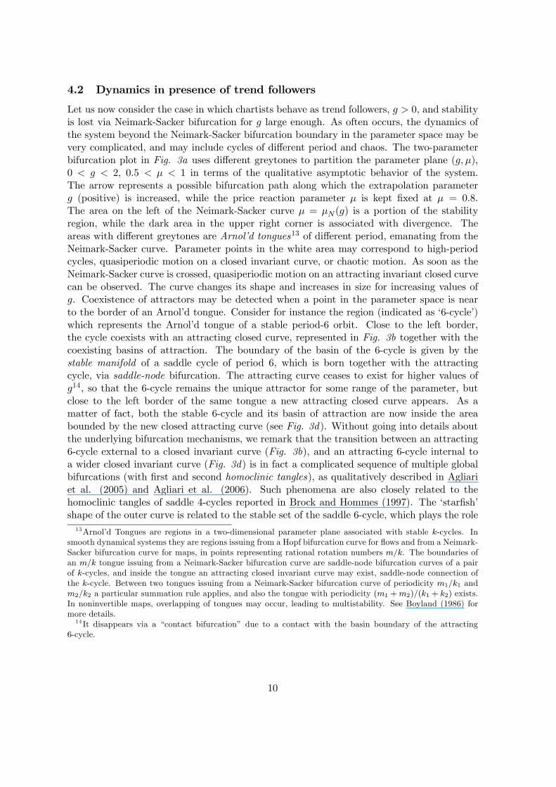
4.2 Dynamics in presence of trend followers

Let us now consider the case in which chartists behave as trend followers, g > 0, and stabilityis lost via Neimark-Sacker bifurcation for g large enough. As often occurs, the dynamics ofthe system beyond the Neimark-Sacker bifurcation boundary in the parameter space may bevery complicated, and may include cycles of different period and chaos. The two-parameterbifurcation plot in Fig. 3a uses different greytones to partition the parameter plane (g, µ),0 < g < 2, 0.5 < µ < 1 in terms of the qualitative asymptotic behavior of the system.The arrow represents a possible bifurcation path along which the extrapolation parameterg (positive) is increased, while the price reaction parameter µ is kept fixed at µ = 0.8.The area on the left of the Neimark-Sacker curve µ = µN (g) is a portion of the stabilityregion, while the dark area in the upper right corner is associated with divergence. Theareas with different greytones are Arnol’d tongues13 of different period, emanating from theNeimark-Sacker curve. Parameter points in the white area may correspond to high-periodcycles, quasiperiodic motion on a closed invariant curve, or chaotic motion. As soon as theNeimark-Sacker curve is crossed, quasiperiodic motion on an attracting invariant closed curvecan be observed. The curve changes its shape and increases in size for increasing values ofg. Coexistence of attractors may be detected when a point in the parameter space is nearto the border of an Arnol’d tongue. Consider for instance the region (indicated as ‘6-cycle’)which represents the Arnol’d tongue of a stable period-6 orbit. Close to the left border,the cycle coexists with an attracting closed curve, represented in Fig. 3b together with thecoexisting basins of attraction. The boundary of the basin of the 6-cycle is given by thestable manifold of a saddle cycle of period 6, which is born together with the attractingcycle, via saddle-node bifurcation. The attracting curve ceases to exist for higher values ofg14, so that the 6-cycle remains the unique attractor for some range of the parameter, butclose to the left border of the same tongue a new attracting closed curve appears. As amatter of fact, both the stable 6-cycle and its basin of attraction are now inside the areabounded by the new closed attracting curve (see Fig. 3d). Without going into details aboutthe underlying bifurcation mechanisms, we remark that the transition between an attracting6-cycle external to a closed invariant curve (Fig. 3b), and an attracting 6-cycle internal toa wider closed invariant curve (Fig. 3d) is in fact a complicated sequence of multiple globalbifurcations (with first and second homoclinic tangles), as qualitatively described in Agliariet al. (2005) and Agliari et al. (2006). Such phenomena are also closely related to thehomoclinic tangles of saddle 4-cycles reported in Brock and Hommes (1997). The ‘starfish’shape of the outer curve is related to the stable set of the saddle 6-cycle, which plays the role13Arnol’d Tongues are regions in a two-dimensional parameter plane associated with stable k-cycles. In

smooth dynamical systems they are regions issuing from a Hopf bifurcation curve for flows and from a Neimark-Sacker bifurcation curve for maps, in points representing rational rotation numbers m/k. The boundaries ofan m/k tongue issuing from a Neimark-Sacker bifurcation curve are saddle-node bifurcation curves of a pairof k-cycles, and inside the tongue an attracting closed invariant curve may exist, saddle-node connection ofthe k-cycle. Between two tongues issuing from a Neimark-Sacker bifurcation curve of periodicity m1/k1 andm2/k2 a particular summation rule applies, and also the tongue with periodicity (m1 +m2)/(k1 + k2) exists.In noninvertible maps, overlapping of tongues may occur, leading to multistability. See Boyland (1986) formore details.14 It disappears via a “contact bifurcation” due to a contact with the basin boundary of the attracting

6-cycle.

10

of basin boundary of the inner attracting periodic orbit.15 The starfish shape of the attractorcauses fluctuations with irregularly varying amplitude (see the black trajectory in Fig. 3e),suggesting clustered volatility at least in a qualitative sense. Moreover, the coexistence ofattractors is itself the source of regimes of fluctuations of different amplitude around theunstable fundamental: this can be seen from the price paths drawn in different greytones inFigs. 3c and 3e (corresponding to the phase plots in Figs. 3b and 3d respectively), generatedby initial conditions taken in different basins of attraction.

By increasing g further, a different phenomenon of coexistence can be observed. Thetongue labelled as ‘13-cycle’ in Fig. 3a, represents in fact a parameter region for which twosymmetric 13-cycles co-exist, as a consequence of the symmetry property (see Section 3.2).These attractors replace the closed invariant curve approximately in the range 1.37488 < g <1.44969. Fig. 3f represents the coexisting cycles, together with their basins of attraction.

The foregoing bifurcation analysis has been carried out by varying two key parameters,under a predefined configuration for the remaining ones. However, we have found (via othersimulations not reported) that the phenomena observed are quite robust with respect toalternative parameter settings. In particular, changes of the parameter s do not affect thequalitative shape of the plots, but only ‘resize’ them to different scales: lower values of s (i.e.higher fundamentalists sensitivity to mispricing) reduce the size of the attractors in Figs. 3band 3d, and the amplitude of fluctuations in Figs. 3c and 3e.

4.3 Stochastic simulations

In this section we present some numerical experiments concerning the noisy dynamical system(12). Fig. 4 represents the time series and the distribution of the returns ρt := (pt − pt−1 +yt)/pt−1 corresponding to different parameter constellations, under i.i.d. dividends and noisetrader demand processes. Both noise trader demand, σ²²t, and dividends, yt, are assumedto be normally distributed, with σ²²t ∼ N (0,σ2²), yt ∼ N (y, s2y), and the same sample pathfor the noise processes is combined with alternative deterministic scenarios.16 Figs. 4a,bcorresponds to the parameter selection of Figs. 3d,e, with strong trend extrapolation bytrend followers and coexistence of attractors in the phase space. The deterministic scenariounderlying Figs. 4c,d is the one depicted in Figs. 2b,c, where chartists behave as contrariansand two different periodic orbits coexist, above and below the unstable fundamental price.Finally, Figs. 4e,f are obtained again for g > 0, but under weaker trend extrapolation andprice reaction than Figs. 4a,b, “inside” the stability domain in the parameter space. Whilein the latter case the return distribution looks approximately normal (Fig. 4f ) and the timeseries resembles a gaussian white noise (Fig. 4e), in the case of strong trend extrapolationthe return distribution is leptokurtic (Fig. 4b), while in the case of contrarian beliefs thedistribution is bimodal (Fig. 4d), and in both cases the time series display volatility clustering(Figs. 4a and 4c). These phenomena may be related to the coexistence of attractors andthe structure of the basins of attraction of the ‘underlying’ deterministic model, though of15The geometric shape of the closed curve follows the unstable set of the saddle cycle, which is characterized

by wide oscillations around the unstable fixed point. This behavior, which is due to the peculiar analyticalform of the map (in particular to the effect of the state-dependent weight α(p) in eq. (13)), can also beobserved from the boundary of the basin of the 6-cycle in Fig.3d. The external closed invariant curve lies nearsuch a basin boundary and therefore assumes the particular starfish shape of Fig.3d.16Note that the average dividend of the simulation is consistent with agents’ expected dividend y := p(R−1).

11

course the connection with the ‘deterministic skeleton’ represents only a naïve way of lookingat the behavior of the noisy model and doesn’t help to provide results about the existence ofa unique limit distribution of prices and returns - which can be thought of as the appropriate‘equilibrium’ notion for such models (see e.g. Böhm and Chiarella (2005), Föllmer, Horst andKirman (2005)).

5 Conclusions

We have developed a two-dimensional discrete-time model of asset price dynamics driven byevolving heterogeneous expectations of two groups of agents, chartists (trend followers orcontrarians) and fundamental traders, under a simple market maker price setting rule. Adistinguishing feature with respect to earlier contributions is one by which the fundamentaltraders possess information about their economic environment (including chartists beliefs)and use this in forming expectations about future prices, nevertheless they put increasingweight on a reversion to fundamental as price deviations from equilibrium become larger.Although this mechanism represents the only nonlinear element within this model, it is ableto keep the model globally stable when the fundamental equilibrium is locally unstable, andso avoids divergent price paths and replaces them by long-run oscillatory behavior alongdifferent, often coexisting attractors, over a wide subset of the parameter space.

Further work on this model needs to be done, in particular the incorporation of time-varying proportions due to switching of traders from chartism to fundamentalism as a conse-quence of the growing belief of a reversion to the fundamental (along the lines of Chiarella-Khomin (2000)), and the explicit introduction of learning schemes which capture the wayfundamental traders can learn about the model structure, including chartists expectations.Furthermore, a more thorough analysis of the noisy model (12) is needed, in particular withregard to the properties of the log-run distributions of prices and returns, under qualitativelydifferent settings for the key behavioural parameters.

AcknowledgementsThis work has been performed with the financial support of MIUR (Italian Ministry of

University and Research) within the scope of the national research project (PRIN 2004)“Nonlinear models in economics and finance: interactions, complexity and forecasting”. Theauthors are grateful to participants at the conferences MDEF 2006 (Urbino, 21-23 September2006), WEHIA 2006 (Bologna, 15-17 June 2006), and Complexity 2006 (Aix en Provence,17-21 May 2006) for remarks and suggestions on earlier drafts of this work, and also wish toacknowledge the helpful comments of two anonymous referees. The usual caveat applies.

Appendix A. Existence and uniqueness of the steady stateIn this Appendix we prove that the fundamental steady state is the unique equilibrium

point of the deterministic map (13).The ‘fundamental’ P ∗ := (p, p), where p = y/(R − 1) is easily recognized as a steady

state, by simply setting (p0, q0) = (p, q) = (p, p), and therefore α(p) = 1, in (13). To see thatno further steady states exist, denote by bP = (bp, bq) = (bp, bp) a generic fixed point of (13),possibly different from P ∗. Then bP must satisfy

bp = bp+ µ A1 [p(R− bα)−Rbp] +A2 [(1 + g −R)bp− gbp+ p(R− 1)]1− µA1bα , (22)

12

where bα := α(bp) = exp £−(p− bp)2/s¤. Condition (22) is easily simplified to:µA1bα(p− bp) = µ(p− bp)[A1R+A2(R− 1)] . (23)

Of course (23) holds for bp = p, while for bp 6= p it is equivalent toα(bp) = R+ A2

A1(R− 1) ,

which admits no solutions because α(bp) ∈ (0, 1], whereas R+ A2A1(R− 1) > R > 1. It follows

that bP = P ∗ is the unique fixed point of (13).Appendix B. Symmetry of the mapIn this Appendix we prove that the symmetry property (20)-(21) holds for any (p, q).

Note first that (21) holds in that it can be rewritten as¡q(S)

¢0= p(S), due to (19). Consider

now (20), and note that from (19) it follows that: (p(S)−p) = (p−p), (p(S)− q(S)) = (q− p),whereas obviously α(p(S)) = α(p). Therefore

F (p(S), q(S)) =

=p(S) + µ

©A1£(p− p(S))R− pα(p(S))¤+A2 £(R− 1)(p− p(S)) + g(p(S) − q(S))¤ª

1− µA1α(p(S))=

=2p− p+ µ A1 [(p− p)R− pα(p)] +A2 [(R− 1)(p− p) + g(q − p)]

1− µA1α(p) =

=2p− 2pα(p)µA11− µA1α(p) − p+ µ A1 [(p− p)R− pα(p)] +A2 [(R− 1)(p− p) + g(p− q)]

1− µA1α(p) =

= 2p− F (p, q) .

13

ReferencesAgliari, A., Bischi, G.I., Dieci, R. & Gardini, L. (2005). Global bifurcations of closed

invariant curves in two-dimensional maps: a computer assisted study. International Journalof Bifurcation and Chaos, 15, 1285-1328.

Agliari, A., Bischi, G.I. & Gardini, L. (2006). Some methods for the global analysis ofclosed invariant curves in two-dimensional maps. (In T. Puu & I. Sushko (Eds.), BusinessCycle Dynamics: Models and Tools (pp. 7-47). Berlin: Springer.)

Boyland, P.L. (1986). Bifurcations of circle maps: Arnold Tongues, bistability and rota-tion intervals. Communications in Mathematical Physics, 106, 353-381.

Böhm, V. & Chiarella, C. (2005). Mean variance preferences, expectations formation andthe dynamics of random asset prices. Mathematical Finance, 15, 61-97.

Brock, W. & Hommes, C.H. (1997). A rational route to randomness. Econometrica, 65,1059-1095.

Brock, W. & Hommes, C.H. (1998). Heterogeneous beliefs and routes to chaos in a simpleasset pricing model. Journal of Economic Dynamics and Control, 22, 1235-1274.

Chiarella, C. (1992). The dynamics of speculative behaviour. Annals of OperationsResearch, 37, 101-123.

Chiarella, C. & He, X.-Z. (2001). Heterogeneous beliefs, risk and learning in a simpleasset pricing model. Computational Economics, 19, 95-132.

Chiarella, C. & He, X.-Z. (2003). Heterogeneous beliefs, risk and learning in a simpleasset pricing model with a market maker. Macroeconomic Dynamics, 7, 503-536.

Chiarella C. & Khomin, A. (2000). The dynamic interaction of rational fundamentalistsand trend chasing chartists in a monetary economy. (In D. Delli Gatti, M. Gallegati & A.Kirman (Eds.), Interaction and Market Structure: Essays on Heterogeneity in Economics(pp. 151-165). Berlin: Springer.)

Day, R.H. & Huang, W. (1990). Bulls, bears and market sheep. Journal of EconomicBehavior and Organization, 14, 299-329.

De Grauwe, P., Dewachter, H. & Embrechts, M. (1993). Exchange rate theories. Chaoticmodels of the foreign exchange market. Oxford: Blackwell.

Föllmer, H., Horst, U. & Kirman, A. (2005). Equilibria in financial markets with het-erogeneous agents: a probabilistic perspective. Journal of Mathematical Economics, 41,123—155.

Gaunersdorfer, A., Hommes, C.H. & Wagener, F. (2003). Bifurcation routes to volatilityclustering under evolutionary learning. Technical Report No. 03-03, CeNDEF, University ofAmsterdam.

Hommes, C.H., Huang, H. & Wang, D. (2005). A robust rational route to randomness ina simple asset pricing model. Journal of Economic Dynamics and Control, 29, 1043-1072.

Hommes, C.H. (2006). Heterogeneous agent models in economics and finance. (In K.L.Judd & L. Tesfatsion (Eds.), Handbook of Computational Economics, Volume 2: Agent-Based Computational Economics (pp. 1109-1186). Amsterdam: North-Holland).

LeBaron, B. (2006). Agent-based Computational Finance. (In K.L. Judd & L. Tesfat-sion (Eds.), Handbook of Computational Economics, Volume 2: Agent-Based ComputationalEconomics (pp. 1187-1234). Amsterdam: North-Holland).

Tong, H. (1990). Nonlinear time-series. A dynamical system approach. Oxford: Claren-don Press.

14

Figure captionsFigure 1. Region of local asymptotic stability of the steady state, in the plane of the

parameters g, µ, and sensitivity of the bifurcation boundaries to the risk-aversion coefficients.Figure 2. Deterministic dynamics with fundamentalists and contrarians. (a) Two-

parameter bifurcation plot for 0 > g > −2, 0 < µ < 1. (b) Coexisting attracting cyclesof period-2 and their basins of attraction. (c) Two time series starting with initial conditionschosen from different basins of attraction.

Figure 3. Deterministic dynamics with fundamentalists and trend followers. (a) Two-parameter bifurcation plot for 0 < g < 2, 0.5 < µ < 1. (b) An attracting closed curve sharingthe phase-plane with an outer attracting orbit of period-6, and (c) two time series startingwith initial conditions chosen from the coexisting basins of attraction. (d) An attracting orbitof period-6 surrounded by a competing “star-fish” attractor, and (e) two time series startingwith initial conditions chosen from different basins. (f) Two symmetric coexisting orbits ofodd period (period-13) with their basins of attraction.

Figure 4. Dynamic outcome of the noisy model, under the same sample paths for thenoise processes, but alternative parameter configurations. (a), (b) Return time series anddistribution under strong trend extrapolation (g = 1.1683, µ = 0.8). (c), (d) Return timeseries and distribution in presence of contrarians (g = −0.85, µ = 0.65). (e), (f) Returntime series and distribution under weaker trend extrapolation (g = 0.5, µ = 0.5). Bothdividends and noise traders’ demand are i.i.d. normal with standard deviations sy = 0.03,σ² = 0.8, respectively. Numerically obtained distributions are based on 6000 observationsafter excluding a transient of 4000 iterations.

15

Figure 1

µ

g

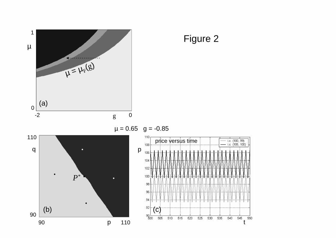
Figure 2

p

q

9090

110

110

g

µ

-2 0

1

0(a)

(b) (c)

µ = 0.65 g = -0.85

µ = µF(g)

P*

price versus time

p

t

Figure 3

g

µ

0 2

1

0.5(a)

(b) (c)

(e)(f)

(d)

µ = 0.8 g = 0.6

µ = 0.8 g = 1.1683µ = 0.8 g = 1.38

p

q

9494

106

106

p

q

8484

116

116

p

q

7878

122

122

13-cy

cle

6-cycle

µ = µN (g)

P*

P*

price versus timep

t

price versus time

p

t

P*

Figure 4

(a) (c) (e)

(b) (d) (f)

return return return

prob

. den

sity

prob

. den

sity

prob

. den

sity

return versus time return versus time return versus time

ρtρt ρt

ttt