A Mixed FSDT Finite-Element Formulation for the Analysis of Composite Laminates Without Shear...
14
A Mixed FSDT Finite-Element Formulation for the Analysis of Composite Laminates Without Shear Correction Factors Ferdinando Auricchio 1 , Elio Sacco 2 , Giuseppe Vairo 3 1 Dipartimento di Meccanica Strutturale Universit`a di Pavia, via Ferrata, 1 27100 Pavia, Italia 2 Dipartimento di Meccanica, Strutture, A&T Universit`a di Cassino, via Di Biasio, 43 03043 Cassino, Italia 3 Dipartimento di Ingegneria Civile Universit`a di Roma “Tor Vergata”, via del Politecnico, 1 00133 Roma, Italia Abstract. A new 4-node finite element for the analysis of laminated plates is developed starting from a partial-mixed FSDT variational formulation, which con- siders out-of-plane shear stresses as primary variables. It does not require either the introduction of shear correction factors or post-processing procedures to ob- tain transverse shear stress profiles. Presented numerical examples show that the element exhibits a quadratic convergence rate and it is locking free. 1 Introduction Laminated composite plates are nowadays widely used in a variety of com- plex structures, especially in space, automotive and civil applications. The main reason for this growing use and development is related to the improve- ment of the ratio between performances and weight for laminated plates with respect to the homogeneous case. However, as a consequence of their anisotropic response, which is characterized by significant shear deformation in the thickness direction and extension-bending coupling, the behaviour of laminated plates is much more complex than homogeneous ones. Actually, several laminate models are available in literature and some of these are also implemented in commercial finite-element codes. Among the various laminate theories the First-order Shear Deformation Theory, de- noted as FSDT, appears to be simple and effective in many structural prob- lems. The main features of this approach, which arises from the classical Reissner–Mindlin assumptions [7,11], are related to the possibility of using C 0 -conforming methods and the ability to capture shear deformations [4]. In this way, it is possible to consider also the case of moderately thick plates [2]. In: Lecture Notes in Applied and Computational Mechanics, vol. 23, p. 345–358, 2005 (Mechanical Modelling and Computational Issues in Civil Engineering), Berlin Heidelberg: Springer-Verlag. doi:10.1007/3-540-32399-6 20. ISBN: 3-540-25567-2, ISSN: 1613-7736
Transcript of A Mixed FSDT Finite-Element Formulation for the Analysis of Composite Laminates Without Shear...
A Mixed FSDT Finite-Element Formulation
for the Analysis of Composite Laminates
Without Shear Correction Factors
Ferdinando Auricchio1, Elio Sacco2, Giuseppe Vairo3
1 Dipartimento di Meccanica StrutturaleUniversita di Pavia, via Ferrata, 127100 Pavia, Italia
2 Dipartimento di Meccanica, Strutture, A&TUniversita di Cassino, via Di Biasio, 4303043 Cassino, Italia
3 Dipartimento di Ingegneria CivileUniversita di Roma “Tor Vergata”, via del Politecnico, 100133 Roma, Italia
Abstract. A new 4-node finite element for the analysis of laminated plates isdeveloped starting from a partial-mixed FSDT variational formulation, which con-siders out-of-plane shear stresses as primary variables. It does not require eitherthe introduction of shear correction factors or post-processing procedures to ob-tain transverse shear stress profiles. Presented numerical examples show that theelement exhibits a quadratic convergence rate and it is locking free.
1 Introduction
Laminated composite plates are nowadays widely used in a variety of com-plex structures, especially in space, automotive and civil applications. Themain reason for this growing use and development is related to the improve-ment of the ratio between performances and weight for laminated plateswith respect to the homogeneous case. However, as a consequence of theiranisotropic response, which is characterized by significant shear deformationin the thickness direction and extension-bending coupling, the behaviour oflaminated plates is much more complex than homogeneous ones.
Actually, several laminate models are available in literature and someof these are also implemented in commercial finite-element codes. Amongthe various laminate theories the First-order Shear Deformation Theory, de-noted as FSDT, appears to be simple and effective in many structural prob-lems. The main features of this approach, which arises from the classicalReissner–Mindlin assumptions [7,11], are related to the possibility of usingC0-conforming methods and the ability to capture shear deformations [4]. Inthis way, it is possible to consider also the case of moderately thick plates [2].
In: Lecture Notes in Applied and Computational Mechanics, vol. 23, p. 345–358, 2005 (Mechanical Modelling and Computational Issues in Civil Engineering), Berlin Heidelberg: Springer-Verlag. doi:10.1007/3-540-32399-6 20. ISBN: 3-540-25567-2, ISSN: 1613-7736
2 F. Auricchio, E. Sacco, G. Vairo
It is worth to observe that the correct use of the FSDT requires the intro-duction of the so-called shear correction factors, which are defined throughthe exact characterization of out-of-plane shear stress profiles. Unfortunately,these latter are known a priori only for homogeneous plates or for simplecases, such as cross-ply laminates under cylindrical bending [6,13,14], whileno closed-form expression is available for more general cases. On the otherhand, shear correction factors have a great influence on the overall structuralresponse. Therefore this aspect represents a clear FSDT’s limitation. As aconsequence, the most FSDT plate and laminate formulations are able torecover satisfactory values of in-plane stresses, while out-of-plane stresses areusually obtained through post-processing of in-plane solution.
In this work, a new 4-node finite element for laminated plates is developedstarting from a partial-mixed FSDT variational formulation, which considersthe out-of-plane shear stresses as primary variables. Through-the-thicknessshear stress profiles, which are introduced to define a suitable functional,are deduced from the three-dimensional local equilibrium equations, i.e. in-tegrating the first two equilibrium equations with respect to the thicknessdirection. Accordingly, shear stresses are expressed as functions of in-planestresses, which can be written as functions either of in-plane strains or ofdisplacement and rotational fields.
The proposed element does not require either the introduction of shearcorrection factors or post-processing procedures in order to obtain out-of-plane stresses. Moreover, a static condensation procedure leads to a finiteelement with only five degrees of freedom per node, as it would be the caseof a classical displacement-based approach. Several numerical examples areperformed for investigating the effectiveness of the proposed formulation andthe main features of the new finite element.
2 FSDT Laminate Model
A laminate plate is a three-dimensional flat body Ω, defined as:
Ω ={(x1, x2, z) ∈ R
3 : z ∈ (−h/2, h/2), (x1, x2) ∈ P ⊂ R2}
. (1)
The laminate is assumed to be formed by � layers perfectly bonded andwhose mechanical properties can be different. The plate thickness h is as-sumed to be constant and the plane z = 0 identifies the mid-plane P ofthe undeformed plate. Top and bottom surfaces of Ω are indicated as P+ =P × {h/2} and P− = P × {−h/2} , respectively. Moreover, the kth layer(index k assumes values in {1, 2, ..., �} ) lies between thickness coordinates zk
and zk+1, such that z1 = −h/2 and z�+1 = h/2.From here onwards the following notation rules are considered, unless
explicitly stated: Greek indices assume values in {1, 2}, whereas Latin indicesassume values in {1, 2, 3} with the exception of index n, which assumes valuesin {1, 2, 3, 4}. Furthermore, partial derivative of f with respect to the in-plane
In: Lecture Notes in Applied and Computational Mechanics, vol. 23, p. 345–358, 2005 (Mechanical Modelling and Computational Issues in Civil Engineering), Berlin Heidelberg: Springer-Verlag. doi:10.1007/3-540-32399-6 20. ISBN: 3-540-25567-2, ISSN: 1613-7736
FSDT FE for Composite Laminates Without Shear Correction Factors 3
coordinate xα is denoted by f,α, whereas partial derivative with respect tothe thickness coordinate z is indicated with an apex, i.e. f ′. Finally, repeatedindices are understood to be summed within their ranges, except for the indexk, which is used to denote any quantity relative to the kth layer.
The FSDT laminate model is based on the following well-known assump-tions on both strain and stress fields [5]: straight lines perpendicular to themid-plane cannot stretch and they remain straight, i.e. ε33 = 0 and ε′α3 = 0;out-of-plane normal stress is zero, i.e. σ33 = 0; out-of-plane shear stresses σα3
are continuous piece-wise quadratic functions of the coordinate z.The previous strain field assumptions lead to the classical representation
form of the displacement field, i.e. as a linear function of the thickness coor-dinate z:
sα(x1, x2, z) = uα(x1, x2) + zϕα(x1, x2) (2)
s3(x1, x2, z) = w(x1, x2). (3)
where uα and w represent the mid-plane displacements and ϕα accounts forthe rotation in the plane xβ = 0 (with β �= α) of perpendicular to mid-planelines.
Hence, the strain tensor can be represented as:
2εαβ = sα,β + sβ,α = 2(eαβ + zκαβ) (4)
2εα3 = s′α + s3,α = ϕα + w,α = γα (5)
ε33 = s′3 = 0 (6)
where γα is the transverse shear strain vector, eαβ = (uα,β + uβ,α)/2 is thein-plane deformation tensor and καβ = (ϕα,β + ϕβ,α)/2 accounts for thecurvature.
The laminated plate is assumed to be formed by linearly elastic monoclinc
layers with symmetry plane parallel to P so that C(k)αβγδ = C
(k)33α3 = 0, where
C(k)ijlm is the fourth-order elasticity tensor for the kth layer. Taking into ac-
count the stress assumptions, the in-plane stress-strain relations for the kthlayer can be written as:
σ(k)αβ = C
(k)
αβγδεγδ = C(k)
αβγδ (eγδ + zκγδ) (7)
where C(k)
is the reduced in-plane elasticity tensor. It can be observed that,since each lamina may present different elastic properties, in-plane stresses
σ(k)αβ are discontinuous piece-wise linear functions of the coordinate z.
As it is well known [5], evaluation of out-of-plane shear stresses τα = σα3
through local constitutive equation is inappropriate, resulting in a stress fieldwhich is not equilibrated at laminae interfaces and which does not generallysatisfy boundary conditions on P+ and P−. On the other hand, an accurateevaluation for τα can be recovered using the three-dimensional equilibrium
4 F. Auricchio, E. Sacco, G. Vairo
equations. No in-plane loads per unit volume as well as tangential surfaceforces on P+ and P− are considered; thus, it results:
τα = σα3 = −
∫ z
−h/2
σαβ,βdζ (8)
where only the boundary condition τα(−h/2) = 0 is automatically enforced,whereas nothing is still said on the condition τα(h/2) = 0.
3 Evaluation of the Shear Stress Profile
Taking into account the representation (7) for the in-plane stress σ(k)αβ and
the equation (8), the shear stress in the kth lamina can be written as:
τ (k)α = τ (k,0)
α −
∫ z
zk
C(k)
αβγδ (eγδ,β + zκγδ,β) dζ (9)
where τ(k,0)α is the shear stress evaluated for z = zk:
τ (k,0)α = −
k−1∑i=1
∫σ
(i)αβ,βdζ = −
(A
(k)αβγδeγδ,β + B
(k)αβγδκγδ,β
)(10)
with
A(k)αβγδ =
k−1∑i=1
(zi+1 − zi)C(i)
αβγδ; B(k)αβγδ =
1
2
k−1∑i=1
(z2i+1 − z2
i )C(i)
αβγδ. (11)
Hence, the expression (9) takes the form:
τ (k)α = −
(A
(k)αβγδeγδ,β + B
(k)αβγδκγδ,β
)(12)
where
A(k)αβγδ(z) = (z − zk)C
(k)
αβγδ + A(k)αβγδ; (13)
B(k)αβγδ(z) =
(z2 − z2k)
2C
(k)
αβγδ + B(k)αβγδ. (14)
In order to enforce the boundary condition τα(h/2) = 0, the expression(12) is enhanced with a linear term in the thickness coordinate z, so that the
shear stress function τ(k)α can be assumed to have the form:
τ (k)α = −
(A
(k)αβγδeγδ,β + B
(k)αβγδκγδ,β
)+ aα(z + h/2) (15)
where the vector aα is solved by the condition τα(h/2) = 0, that is:
aα =1
h(Aαβγδeγδ,β + Bαβγδκγδ,β) (16)
In: Lecture Notes in Applied and Computational Mechanics, vol. 23, p. 345–358, 2005 (Mechanical Modelling and Computational Issues in Civil Engineering), Berlin Heidelberg: Springer-Verlag. doi:10.1007/3-540-32399-6 20. ISBN: 3-540-25567-2, ISSN: 1613-7736
FSDT FE for Composite Laminates Without Shear Correction Factors 5
with
Aαβγδ = A(�)αβγδ
∣∣∣z= h
2
=
�∑k=1
(zk+1 − zk)C(k)
αβγδ; (17)
Bαβγδ = B(�)αβγδ
∣∣∣z= h
2
=1
2
�∑k=1
(z2k+1 − z2
k)C(k)
αβγδ. (18)
It is worth to observe that Aαβγδ and Bαβγδ are the classical laminatemembrane and membrane-bending coupling fourth-order in-plane elasticitytensors. They do not depend either on the thickness coordinate z or on thespecific lamina.
Finally, substituting the expression (16) into the equation (15), shearstresses can be represented putting in evidence the explicit dependency onthe thickness coordinate z:
τ (k)α (z) = −
[(A
(k,0)αβγδ + zA
(k,1)αβγδ
)eγδ,β +
(B
(k,0)αβγδ + zB
(k,1)αβγδ + z2B
(k,2)αβγδ
)κγδ,β
](19)
where the following fourth-order in-plane tensors are introduced:{A(k,0) = A(k) − zkC
(k)− 1
2A
A(k,1) = C(k)
− 1hA
⎧⎪⎨⎪⎩B(k,0) = B(k) − z2
k
2 C(k)
− 12B
B(k,1) = − 1hB
B(k,2) = 12C
(k).
(20)
4 Variational Formulation
The following mixed functional is considered:
Π(εαβ , σαβ , σα3, sα) = Π(mb)(εαβ , σαβ , sα) + Π(s)(σα3, sα) − Πext (21)
where Π(mb) accounts for membrane-bending terms, Π(s) accounts for trans-verse shear terms and Πext accounts for boundary and loading conditions. Indetail, Π(mb) has a Hu–Washizu-like form and it is defined as:
Π(mb) =1
2
∫Ω
Cαβγδεαβεγδdv +
∫Ω
σαβ
[(sα,β + sβ,α
2
)− εαβ
]dv
=1
2
∫Ω
Cαβγδ(eαβ + zκαβ)(eγδ + zκγδ)dv (22)
+
∫Ω
σαβ
2
[(uα + zϕα),β + (uβ + zϕβ),α − 2 (eαβ + zκαβ)
]dv
while Π(s) has an Hellinger–Reissner-like form and it is defined as:
Π(s) =
∫Ω
τα(w,α + ϕα)dv −1
2
∫Ω
Tαβτατβdv (23)
6 F. Auricchio, E. Sacco, G. Vairo
where Tαβ = C−1α3β3 represents the compliance shear elastic tensor.
Performing the integration along the thickness coordinate z, the membra-ne-bending part Π(mb) of the functional (21) can be written as:
Π(mb) =1
2
∫P
(Aαβγδeαβeγδ + 2Bαβγδeαβκγδ + Dαβγδκαβκγδ) dA
+
∫P
Nαβ
[(uα,β + uβ,α
2
)− eαβ
]dA (24)
+
∫P
Mαβ
[(ϕα,β + ϕβ,α
2
)− καβ
]dA
where Dαβγδ =∑�
i=1(z3i+1−z3
i )C(k)
αβγδ/3 is the fourth-order in-plane laminate
bending elasticity tensor, Nαβ =∫ h/2
−h/2σαβdz is the in-plane resultant force
tensor and Mαβ =∫ h/2
−h/2zσαβdz is the bending moment one.
Moreover, noting that the quantity (w,α + ϕα) is constant with referenceto the thickness coordinate z, the first term of Π(s) can be written as:∫
Ω
τα(w,α + ϕα)dv =
∫P
Sα(w,α + ϕα)dA (25)
where the resulting shear force Sα is introduced:
Sα =
∫ h/2
−h/2
ταdz =
�∑k=1
∫ zk+1
zk
τ (k)α dz = −
[Z
(e)αβγδeγδ,β + Z
(κ)αβγδκγδ,β
](26)
with
Z(e)αβγδ =
�∑k=1
2∑i=1
(zik+1 − zi
k)
iA
(k,i−1)αβγδ ; (27)
Z(κ)αβγδ =
�∑k=1
3∑i=1
(zik+1 − zi
k)
iB
(k,i−1)αβγδ . (28)
Similarly, recalling the expression (19), formal integration through thethickness for the second term of Π(s) leads to:
∫Ω
Tαβτατβdv =
∫P
�∑k=1
∫ zk+1
zk
T(k)
αβ τ (k)α τ
(k)β dz dA
=
∫P
(Π(s,ee) + 2Π(s,eκ) + Π(s,κκ)
)dA (29)
In: Lecture Notes in Applied and Computational Mechanics, vol. 23, p. 345–358, 2005 (Mechanical Modelling and Computational Issues in Civil Engineering), Berlin Heidelberg: Springer-Verlag. doi:10.1007/3-540-32399-6 20. ISBN: 3-540-25567-2, ISSN: 1613-7736
FSDT FE for Composite Laminates Without Shear Correction Factors 7
where
Π(s,ee) =
�∑k=1
3∑i=1
(zik+1 − zi
k)
ig(k,i);
Π(s,eκ) =�∑
k=1
4∑i=1
(zik+1 − zi
k)
im(k,i); (30)
Π(s,κκ) =
�∑k=1
5∑i=1
(zik+1 − zi
k)
ip(k,i).
Introduced quantities in (30) are defined as:
g(k,i) =∑q,r
T(k)
αβ
(A
(k,q)αγδζeδζ,γ
) (A
(k,r)βϑλμeλμ,ϑ
)q, r ∈ SA
m(k,i) =∑q,r
T(k)
αβ
(A
(k,q)αγδζeδζ,γ
)(B
(k,r)βϑλμκλμ,ϑ
)q ∈ SA, r ∈ SB (31)
p(k,i) =∑q,r
T(k)
αβ
(B
(k,q)αγδζκδζ,γ
)(B
(k,r)βϑλμκλμ,ϑ
)q, r ∈ SB
where SA = {0, 1}; SB = {0, 1, 2} and symbol∑
q,r denotes summation onevery combination of q and r which satisfies the condition i = (q + r +1), fora fixed value of i.
Therefore, in accordance with the conditions (26) and (29), the functionalΠ(s) can be written as:
Π(s) = −
∫P
[Z
(e)αβγδeγδ,β + Z
(κ)αβγδκγδ,β
](w,α + ϕα) dA
−1
2
∫P
(Π(s,ee) + 2Π(s,eκ) + Π(s,κκ)
)dA (32)
as well as the functional Π introduced in (21) becomes:
Π = Π(mb)(eαβ , καβ , uα, ϕα,Nαβ ,Mαβ)+Π(s)(eαβ , καβ , ϕα, w)−Πext (33)
where both Π(mb) and Π(s) are referred to the two-dimensional plate mid-surface P. The field and boundary laminate governing equations are deducedperforming the stationary conditions of Π with respect to the parameterseαβ , καβ , uα, ϕα, w, Nαβ and Mαβ .
5 The Finite Element
A four-node laminate finite element is obtained performing the discretizationof the functional (33) and considering a standard iso-parametric map [15]:
xα = Ψn(xα)n (34)
8 F. Auricchio, E. Sacco, G. Vairo
where xα is the global in-plane coordinate vector in the physical element,Ψn(ξ1, ξ2) = (1+ ξ1nξ1)(1+ ξ2nξ2) are the standard bi-linear shape functions,ξα is the parent element coordinate vector and (xα)n is the in-plane coordi-nate vector for the node n. Notation ( · )n indicates a nodal quantity for thenode n.
The following interpolation schemes for the displacement fields are intro-duced:
- the in-plane displacement interpolation is bi-linear in the nodal parame-ters uα, i.e. uα = Ψn(uα)n;
- the transverse displacement interpolation is bi-linear in the nodal para-meters wn and it is enriched with linked quadratic functions in terms ofnodal rotations (ϕα)n. In detail, following [1] it results:
w = Ψnwn + Ψ (wϕ)n
Ln
16(ϕo
n − ϕos) (35)
where ϕon and ϕo
s are the components of the n and s node rotations inthe direction normal to the n− s side, whose length is Ln. Furthermore,
the shape functions Ψ(wϕ)n are set as:⎧⎪⎪⎪⎨⎪⎪⎪⎩
Ψ(wϕ)1 = (1 − ξ2
1)(1 − ξ2)
Ψ(wϕ)2 = (1 + ξ1)(1 − ξ2
2)
Ψ(wϕ)3 = (1 − ξ2
1)(1 + ξ2)
Ψ(wϕ)4 = (1 − ξ1)(1 − ξ2
2)
; (36)
- the rotational field is bi-linear in the nodal parameters ϕn with added
internal degrees of freedom ϕ(b)n , i.e. ϕα = Ψn(ϕα)n +Ψ
(b)αn ϕ
(b)n , where Ψ
(b)αn
are bubble functions defined as [1]:[Ψ (b)
αn
]=
(1 − ξ21)(1 − ξ2
2)
det[J]
[Jo
22 −Jo12 Jo
22ξ2 −Jo12ξ1
−Jo21 Jo
11 −Jo21ξ2 Jo
11ξ1
](37)
where Jαβ = ∂xα/∂ξβ is the jacobian of the iso-parametric map andJo
αβ = Jαβ |ξ1=ξ2=0.
Moreover, the following interpolation schemes are adopted for the remain-ing fields:⎧⎪⎪⎪⎨⎪⎪⎪⎩
eαβ = Ψ(e)n (eαβ)n
καβ = Ψ(κ)n (καβ)n
Nαβ = Ψ(N )n (Nαβ)n
Mαβ = Ψ(M)n (Mαβ)n
(38)
where Ψ(e)n , Ψ
(κ)n , Ψ
(N )n , Ψ
(M)n are proper interpolation functions. In this work
they are set equal to piece-wise discontinuous linear functions and such that:
Ψ (e)n = Ψ (κ)
n = Ψ (N )n = Ψ (M)
n . (39)
In: Lecture Notes in Applied and Computational Mechanics, vol. 23, p. 345–358, 2005 (Mechanical Modelling and Computational Issues in Civil Engineering), Berlin Heidelberg: Springer-Verlag. doi:10.1007/3-540-32399-6 20. ISBN: 3-540-25567-2, ISSN: 1613-7736
FSDT FE for Composite Laminates Without Shear Correction Factors 9
It can be observed that the degrees of freedom (ϕ(b))n, (eαβ)n, (καβ)n,
(Mαβ)n and (Nαβ)n are local to each element and consequently they canbe statically condensed element-by-element.
Introducing the proposed interpolation schemes, the functional (33) maybe arranged in a discrete form as a function of the unknown nodal parameters.As an example, the resultant shear force Sα, which has been introduced in(26), may be expressed as:
Sα = −[Z
(e)αβγδΨ
(e)n,β(eγδ)n + Z
(κ)αβγδΨ
(κ)n,β(κγδ)n
]=
(S
(e)αγδ
)n
(eγδ)n +(S
(κ)αγδ
)n
(κγδ)n (40)
where (S(e)αγδ)n = −Z
(e)αβγδΨ
(e)n,β and (S
(κ)αγδ)n − Z
(κ)αβγδΨ
(κ)n,β can be interpreted
as new interpolation functions.
The element balance equation is deduced performing the functional sta-tionary conditions for a single element and statically condensing the internaldegrees of freedom.
In this way, although the use of a mixed formulation is associated to anincrease of fields to be interpolated, a finite element with only five degreesof freedom per node is obtained, as it would be the case of the classicaldisplacement-based approach.
6 Numerical Examples
The proposed laminate element has been implemented in FEAP (Finite Ele-ment Analysis Program) [12] and several numerical examples are investigatedin order to assess its performances.
In the following, the new element is denoted as EML4S and it is comparedwith the laminate finite-element EML4, which has been proposed in [2]. Indetail, the element EML4 is based on an iterative technique for the correctevaluation of the shear correction factors. The EML4’s solution at the begin-ning of the iterative procedure is indicated as EML4(i) and it correspondsto the classical Reissner–Mindlin theory with direct shear factors set equalto 5/6, whereas the EML4’s solution at the end of the iterative procedure isindicated as EML4(f).
Computations are developed considering square cross-ply laminates withside length L and several side-to-thickness ratios η = L/h. The plates aresubjected to a sinusoidal distributed load q = qo sin(φx1) sin(φx2), with φ =π/L, and they are assumed to be simply supported along their boundaries:
s2 = 0, s3 = 0, ϕ2 = 0 at x1 = 0, x1 = L;
s1 = 0, s3 = 0, ϕ1 = 0 at x2 = 0, x2 = L.
10 F. Auricchio, E. Sacco, G. Vairo
Moreover, the laminae are assumed to be orthotropic with properties cor-responding to an high modulus graphite/epoxy composite:
EL
ET= 25, νTT = 0. 25,
GLT
ET= 0. 5,
GTT
ET= 0. 2
where E refers to the elasticity moduli, G to the shear moduli and ν to thePoisson’s ratios. Furthermore, the subscript L refers to the along-the-fiberdirection, whereas the subscript T refers to any orthogonal-to-fiber direction.
The numerical analyses are performed using regular meshes based onsquare elements and the relevant results are compared with:
- the classical FSDT analytical solution [9], with direct shear correctionfactors set equal to 5/6 (denoted as FSDT5/6);
- the classical FSDT analytical solution, with shear correction factors setas suggested by Whitney in [14] (denoted as FSDTW );
- the analytical solution for the proposed refined FSDT model (denoted asFSDTR);
- the exact three-dimensional solution proposed by Pagano [8] (denoted as3D-AS).
Three different cross-ply lamination sequences are considered: the sym-metrical 0/90/0 one, the unsymmetrical 0/90 and 90/0/90/0 ones.
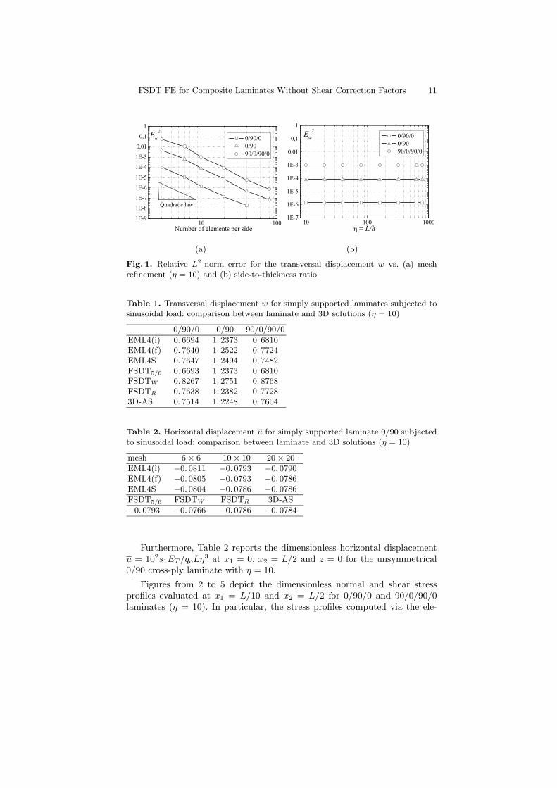
Figure 1 shows the relative error for the transverse displacement field wversus (a) the number of nodes per side (with η = 10) and (b) versus theside-to-thickness ratio η.
In detail, the relative error for the discrete solution is measured as:
E2w =
∑N [w�(x1N , x2N ) − w(x1N , x2N )]
2∑N w(x1N , x2N )2
(41)
where the sum is performed over all the nodal points, w(x1N , x2N ) denotesthe value of w at the coordinate of node N and it is given by the analyticalsolution FSDTR, whereas w�(x1N , x2N ) is the value obtained by numericalcomputation and corresponding to a mesh parameter �. It is worth to ob-serve that the above-mentioned error measure can be intended as a discreteL2−type error.
It turns out that element EML4S is characterized by a quadratic conver-gence rate (in Fig. 1a the theoretical L2-convergence slope is also indicated)and it does not exhibit locking phenomena.
Table 1 reports the dimensionless transverse displacement w at the platecenter for the three analysed cross-ply lamination sequences. It is defined asw = 102wET /qoLη3. Comparison between the EML4S’s numerical solutionsand the reference ones (numerically and analytically obtained) is performed.The numerical solutions are computed employing regular meshes of 10 × 10elements and setting η = 10.
In: Lecture Notes in Applied and Computational Mechanics, vol. 23, p. 345–358, 2005 (Mechanical Modelling and Computational Issues in Civil Engineering), Berlin Heidelberg: Springer-Verlag. doi:10.1007/3-540-32399-6 20. ISBN: 3-540-25567-2, ISSN: 1613-7736
FSDT FE for Composite Laminates Without Shear Correction Factors 11
(a) (b)
Fig. 1. Relative L2-norm error for the transversal displacement w vs. (a) meshrefinement (η = 10) and (b) side-to-thickness ratio
Table 1. Transversal displacement w for simply supported laminates subjected tosinusoidal load: comparison between laminate and 3D solutions (η = 10)
0/90/0 0/90 90/0/90/0
EML4(i) 0. 6694 1. 2373 0. 6810EML4(f) 0. 7640 1. 2522 0. 7724EML4S 0. 7647 1. 2494 0. 7482FSDT5/6 0. 6693 1. 2373 0. 6810FSDTW 0. 8267 1. 2751 0. 8768FSDTR 0. 7638 1. 2382 0. 77283D-AS 0. 7514 1. 2248 0. 7604
Table 2. Horizontal displacement u for simply supported laminate 0/90 subjectedto sinusoidal load: comparison between laminate and 3D solutions (η = 10)
mesh 6 × 6 10 × 10 20 × 20
EML4(i) −0. 0811 −0. 0793 −0. 0790EML4(f) −0. 0805 −0. 0793 −0. 0786EML4S −0. 0804 −0. 0786 −0. 0786
FSDT5/6 FSDTW FSDTR 3D-AS
−0. 0793 −0. 0766 −0. 0786 −0. 0784
Furthermore, Table 2 reports the dimensionless horizontal displacementu = 102s1ET /qoLη3 at x1 = 0, x2 = L/2 and z = 0 for the unsymmetrical0/90 cross-ply laminate with η = 10.
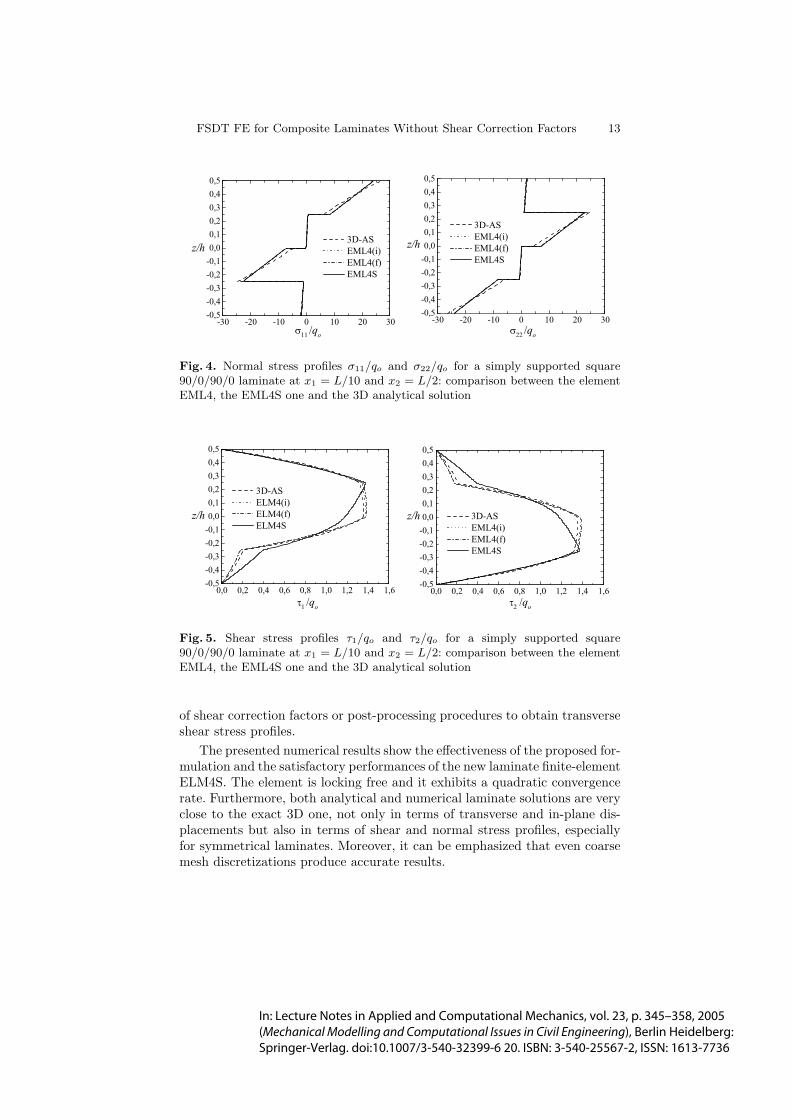
Figures from 2 to 5 depict the dimensionless normal and shear stressprofiles evaluated at x1 = L/10 and x2 = L/2 for 0/90/0 and 90/0/90/0laminates (η = 10). In particular, the stress profiles computed via the ele-
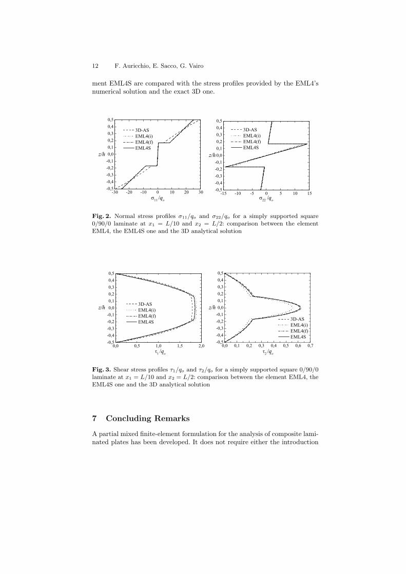
12 F. Auricchio, E. Sacco, G. Vairo
ment EML4S are compared with the stress profiles provided by the EML4’snumerical solution and the exact 3D one.
Fig. 2. Normal stress profiles σ11/qo and σ22/qo for a simply supported square0/90/0 laminate at x1 = L/10 and x2 = L/2: comparison between the elementEML4, the EML4S one and the 3D analytical solution
Fig. 3. Shear stress profiles τ1/qo and τ2/qo for a simply supported square 0/90/0laminate at x1 = L/10 and x2 = L/2: comparison between the element EML4, theEML4S one and the 3D analytical solution
7 Concluding Remarks
A partial mixed finite-element formulation for the analysis of composite lami-nated plates has been developed. It does not require either the introduction
FSDT FE for Composite Laminates Without Shear Correction Factors 13
Fig. 4. Normal stress profiles σ11/qo and σ22/qo for a simply supported square90/0/90/0 laminate at x1 = L/10 and x2 = L/2: comparison between the elementEML4, the EML4S one and the 3D analytical solution
Fig. 5. Shear stress profiles τ1/qo and τ2/qo for a simply supported square90/0/90/0 laminate at x1 = L/10 and x2 = L/2: comparison between the elementEML4, the EML4S one and the 3D analytical solution
of shear correction factors or post-processing procedures to obtain transverseshear stress profiles.
The presented numerical results show the effectiveness of the proposed for-mulation and the satisfactory performances of the new laminate finite-elementELM4S. The element is locking free and it exhibits a quadratic convergencerate. Furthermore, both analytical and numerical laminate solutions are veryclose to the exact 3D one, not only in terms of transverse and in-plane dis-placements but also in terms of shear and normal stress profiles, especiallyfor symmetrical laminates. Moreover, it can be emphasized that even coarsemesh discretizations produce accurate results.
In: Lecture Notes in Applied and Computational Mechanics, vol. 23, p. 345–358, 2005 (Mechanical Modelling and Computational Issues in Civil Engineering), Berlin Heidelberg: Springer-Verlag. doi:10.1007/3-540-32399-6 20. ISBN: 3-540-25567-2, ISSN: 1613-7736
14 F. Auricchio, E. Sacco, G. Vairo
The little disagreement of the ELM4S’s solutions with respect to theELM4’s and analytical ones in the case of unsymmetrical laminates (cf. fi-gure 5) may be attributed to the choices (38) and (39). However, it shouldbe solved through an enhancement of the interpolation schemes which havebeen adopted for the auxiliary fields. Therefore, this aspect represents a futureguide-line for further development of the proposed laminate finite-element.
Acknowledgements
This research was developed within the framework of Lagrange Laboratory,an European research group between CNRS, CNR, University of Rome “TorVergata”, University of Montpellier II, ENPC and LCPC.
References
1. Auricchio F., Taylor R. (1994) A shear-deformable plate element with an exactthin limit, Comp. Meth. App. Mech. Engrg. 118, 393-412.
2. Auricchio F., Sacco E. (1999) A mixed-enhanced finite element for the analysisof laminated composite plates, Int. J. Numer. Methods Engrg. 44, 1481-1504.
3. Auricchio F., Sacco E. (1999) Partial-mixed formulation and refined models forthe analysis of composite laminates within an FSDT, Comp. Struct. 46, 103-113.
4. Auricchio F., Lovadina C., Sacco E. (2001) Analysis of mixed finite elements forlaminated composite plates, Comput. Methods Appl. Mech. Engrg. 190, 4767-4783.
5. Bisegna P., Sacco E. (1996) A rational deduction of plate theories from the three-dimensional linear elasticity, Zeit. fur angew. math. und mech. 77, 349-366.
6. Laitinen M., Lahtinen H., Sjolind S. G. (1995) Transverse shear correction factorsfor laminates in cylindrical bending, Commun. Num. Meth. Eng. 11, 41-47.
7. Mindlin R. D. (1951) Influence of rotatory inertia and shear on flexural motionsof isotropic, elastic plates, J. App. Mech. 38, 31-38.
8. Pagano N. J. (1979) Exact solutions for rectangular bidirectional composites andsandwich plates, J. Comp. Mater. 4, 20-34.
9. Reddy J. N. (1984) Energy and variational methods in applied mechanics, NewYork, Wiley.
10. Reddy J. N. (1997) Mechanics of Laminated Composite Plates - Theory andAnalysis, CRC Press, Boca Raton.
11. Reissner E. (1945) The effect of transverse shear deformation on the bendingof elastic plates, J. App. Mech. 12, 69-77.
12. Taylor R. (2000) A finite-element analysis program. Technical report, Univ. ofCalifornia at Berkeley.
13. Vlachoutsis S. (1992) Shear correction factors for paltes and shell, Int. J. Num.Meth. Eng. 33, 1537-1552.
14. Whitney J. M. (1973) Shear correction factors for orthotropic laminates understatic load, J. Appl. Mech. 40, 302-304.
15. Zienkiewicz O. C., Taylor R. L. (1997) The Finite Element Method, vol. 1, 4thEd., McGraw-Hill.
In: Lecture Notes in Applied and Computational Mechanics, vol. 23, p. 345–358, 2005 (Mechanical Modelling and Computational Issues in Civil Engineering), Berlin Heidelberg: Springer-Verlag. doi:10.1007/3-540-32399-6 20. ISBN: 3-540-25567-2, ISSN: 1613-7736