A Method for Reducing Ill-Conditioning of Polynomial Root ...
15
Portland State University Portland State University PDXScholar PDXScholar University Honors Theses University Honors College 2014 A Method for Reducing Ill-Conditioning of A Method for Reducing Ill-Conditioning of Polynomial Root Finding Using a Change of Basis Polynomial Root Finding Using a Change of Basis Edison Tsai Portland State University Follow this and additional works at: https://pdxscholar.library.pdx.edu/honorstheses Let us know how access to this document benefits you. Recommended Citation Recommended Citation Tsai, Edison, "A Method for Reducing Ill-Conditioning of Polynomial Root Finding Using a Change of Basis" (2014). University Honors Theses. Paper 109. https://doi.org/10.15760/honors.113 This Thesis is brought to you for free and open access. It has been accepted for inclusion in University Honors Theses by an authorized administrator of PDXScholar. Please contact us if we can make this document more accessible: [email protected].
-
Upload
khangminh22 -
Category
Documents
-
view
0 -
download
0
Transcript of A Method for Reducing Ill-Conditioning of Polynomial Root ...
Portland State University Portland State University
PDXScholar PDXScholar
University Honors Theses University Honors College
2014
A Method for Reducing Ill-Conditioning of A Method for Reducing Ill-Conditioning of
Polynomial Root Finding Using a Change of Basis Polynomial Root Finding Using a Change of Basis
Edison Tsai Portland State University
Follow this and additional works at: https://pdxscholar.library.pdx.edu/honorstheses
Let us know how access to this document benefits you.
Recommended Citation Recommended Citation Tsai, Edison, "A Method for Reducing Ill-Conditioning of Polynomial Root Finding Using a Change of Basis" (2014). University Honors Theses. Paper 109. https://doi.org/10.15760/honors.113
This Thesis is brought to you for free and open access. It has been accepted for inclusion in University Honors Theses by an authorized administrator of PDXScholar. Please contact us if we can make this document more accessible: [email protected].
A Method for Reducing Ill-Conditioning of Polynomial
Root Finding Using a Change of Basis
by
Edison Tsai
An undergraduate honors thesis submitted in partial fulfillment of the
requirements for the degree of
Bachelor of Science
in
University Honors
and
Mathematics
Thesis Adviser
Dr. Jeffrey Ovall
Portland State University
2014
1. A Brief History of Polynomial Root Finding The problem of solving polynomial equations is one of the oldest problems in
mathematics. Many ancient civilizations developed systems of algebra which included methods
for solving linear equations. Around 2000 B.C.E. the Babylonians found a method for solving
quadratic equations which is equivalent to the modern quadratic formula. They also discovered a
method for approximating square roots which turned out to be a special case of Newton’s
method (which was not discovered until over 3500 years later). Several Italian Renaissance
mathematicians found general methods for finding roots of cubic and quartic polynomials. But it
is known that there is no general formula for finding the roots of any polynomial of degree 5 or
higher using only arithmetic operations and root extraction. Therefore, when presented with the
problem of solving a fifth degree or higher polynomial equation, it is necessary to resort to
numerical approximations. In fact, even for third and fourth degree polynomials, it is usually
much better in practice to use numerical methods because the exact formulas are extremely prone
to round-off errors.
One of the most well-known numerical methods for solving not only polynomial
equations, but for finding roots of any sufficiently well-behaved function in general, is Newton’s
method. In certain cases, however, such as in the case of repeated roots, Newton’s method, as
well as many other iterative methods, do not work very well because the convergence is much
slower. In addition, iterative methods exhibit sensitive dependence on initial conditions, so that it
is essentially impossible to predict beforehand which root an iterative method will converge to
for a given initial condition.
Even if one had a method for finding all roots of a given polynomial with unlimited
accuracy, there is another fundamental obstacle in the problem of finding roots of polynomials.
The problem is that most polynomials exhibit a phenomenon known as ill-conditioning, so that a
small perturbation to the coefficients of the polynomial can result in large changes in the roots.
In general, when attempting to derive numerical approximations to the solution of any
mathematical problem (not just finding polynomial roots) it is prudent to avoid ill-conditioning
because it can increase sensitivity to round-off errors.
2. The Problem of Ill-Conditioning Ill-conditioning is a phenomenon which appears in many mathematical problems and
algorithms including polynomial root finding. Other examples of ill-conditioned problems
include finding the inverse of a matrix with a large condition number or computing the
eigenvalues of a large matrix. In many cases, whether or not a given problem is ill-conditioned
depends on the algorithm used to solve the problem. For example, computing the QR
factorization of a matrix can be ill-conditioned if one naively applies the Gram-Schmidt
orthogonalization procedure in the most straightforward way, but using Householder reflections
to compute a QR factorization is numerically stable and much less prone to round-off errors.
A classic example of ill-conditioning in the context of finding polynomial roots is the so-
called Wilkinson polynomial. This polynomial is defined by
(1)
Clearly, by definition the roots of this polynomial are the integers from 1 to 20. The expanded
form of the product in equation (1) may be given as
where the coefficients ci are given by
and sj denotes the jth
elementary symmetric polynomial (with the convention that s0 is identically
1). It would be most convenient if a small change to any of the coefficients ci resulted in a
similarly small change to the roots of the polynomial. Unfortunately, this is far from the case.
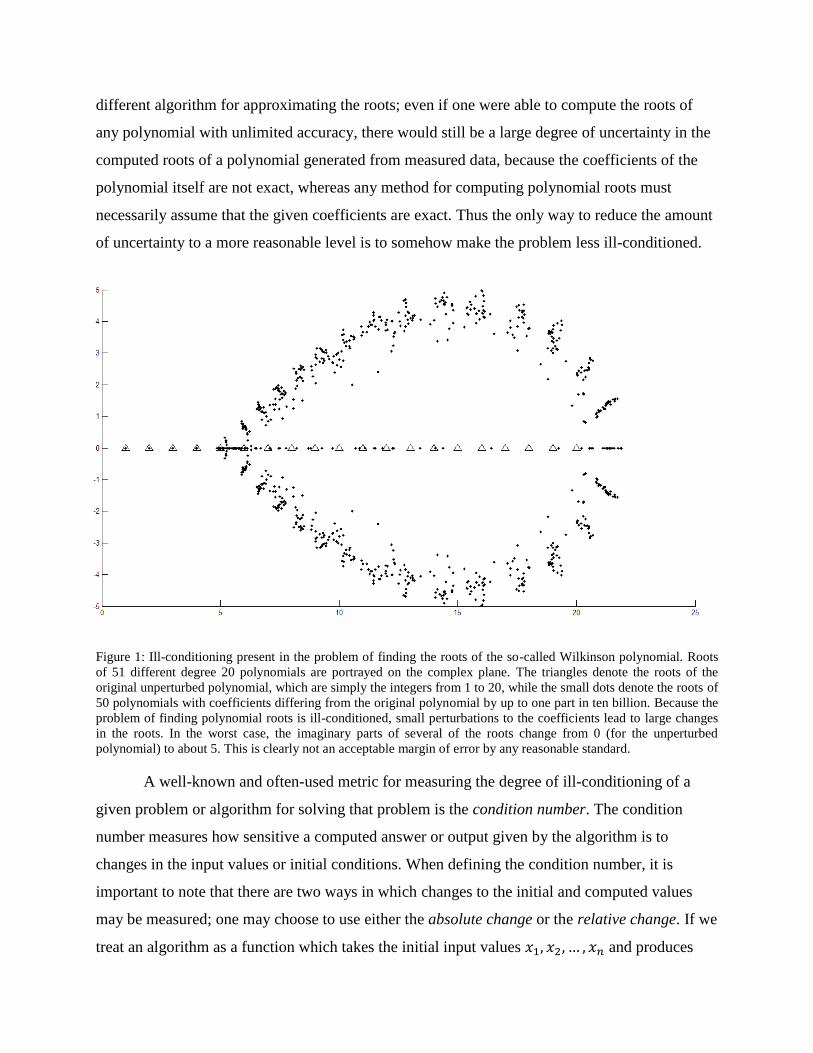
Figure 1 shows the roots of 50 different polynomials which differ from the polynomial
given by equation (2) only in that each of the coefficients ci has been perturbed by a random
amount up to 10-10
of the original value (i.e. by up to one part in ten billion). We see that
although the change in the coefficients is very small by any standard, the effect on the roots is
quite drastic. The problem is made worse by the fact that in most, if not all, real world
applications, where polynomials are used to model or interpolate data, there will be some
uncertainty in the values of the coefficients, arising from uncertainties in whatever measurements
are used to generate the data. When the polynomial is ill-conditioned, as in the preceding
example, very small uncertainties in the coefficients can lead to large uncertainties in the roots,
often many orders of magnitude larger. This issue cannot be resolved simply by choosing a
different algorithm for approximating the roots; even if one were able to compute the roots of
any polynomial with unlimited accuracy, there would still be a large degree of uncertainty in the
computed roots of a polynomial generated from measured data, because the coefficients of the
polynomial itself are not exact, whereas any method for computing polynomial roots must
necessarily assume that the given coefficients are exact. Thus the only way to reduce the amount
of uncertainty to a more reasonable level is to somehow make the problem less ill-conditioned.
Figure 1: Ill-conditioning present in the problem of finding the roots of the so-called Wilkinson polynomial. Roots
of 51 different degree 20 polynomials are portrayed on the complex plane. The triangles denote the roots of the
original unperturbed polynomial, which are simply the integers from 1 to 20, while the small dots denote the roots of
50 polynomials with coefficients differing from the original polynomial by up to one part in ten billion. Because the
problem of finding polynomial roots is ill-conditioned, small perturbations to the coefficients lead to large changes
in the roots. In the worst case, the imaginary parts of several of the roots change from 0 (for the unperturbed
polynomial) to about 5. This is clearly not an acceptable margin of error by any reasonable standard.
A well-known and often-used metric for measuring the degree of ill-conditioning of a
given problem or algorithm for solving that problem is the condition number. The condition
number measures how sensitive a computed answer or output given by the algorithm is to
changes in the input values or initial conditions. When defining the condition number, it is
important to note that there are two ways in which changes to the initial and computed values
may be measured; one may choose to use either the absolute change or the relative change. If we
treat an algorithm as a function which takes the initial input values and produces
outputs , then the condition number of the jth
output yj with respect to the ith
input xi
measures how large of a change in yj can result from a small perturbation of xi. If we denote a
small perturbation of xi by , then the absolute change in xi is simply , whereas the relative
change is defined by . Thus the absolute change only measures the numerical difference
between the perturbed and original values of a variable, whereas the relative change measures
the perturbation as a proportion of the variable’s original value. . Usually, in numerical analysis
the relative change is more important because the floating-point arithmetic system used by
computers has a fixed amount of precision on a relative basis; i.e. in floating-point arithmetic an
error margin of ±10 for a computed value of 1000 is just as precise as an error margin of ±1 for a
computed value of 100.
We think of an algorithm for solving a problem as a function from an arbitrary set X, the
set of parameters or initial conditions, to a set Y, the set of solutions. In order to define the
condition number, we require that the notion of distance between two elements exists in both the
set of initial conditions and the set of solutions; thus we assume that X and Y are normed vector
spaces. In the case of polynomial root-finding, X and Y are both vectors of complex numbers: X
consists of the polynomial coefficients, and Y consists of the roots.
Definition: given a function where X and Y are normed vector spaces, the
absolute condition number of f at any is defined by
and the relative condition number of f at is defined by
We wish to obtain an expression for the condition number of a root of a polynomial with
respect to a given coefficient. Here, we are treating the roots of the polynomial as a function of
the coefficients, and working in the vector space . However, we are only interested in the
sensitivity of any particular root to changes in one particular coefficient at a time. Therefore, we
may think of the jth
root as being a function of the ith
coefficient, holding all other coefficients
fixed. In this case we may then refer to the (relative) condition number of the jth
root with respect
to the ith
coefficient, this being defined as the relative condition number of the function (which
gives the jth
root in terms of the ith
coefficient) at the ith
coefficient.
The following theorem provides an expression for computing the condition number of
any root with respect to any coefficient, provided that the root has multiplicity 1. Note that the
condition number of a multiple root is always infinite because the derivative of a polynomial at a
multiple root is 0, so that small changes to any coefficient can lead to arbitrarily large changes in
the roots.
Theorem 1: Let be a degree n polynomial with coefficients ci for
. If r is a nonzero root of p(x) with multiplicity 1, and , then the relative
condition number of r with respect to cj is
Proof: Let be any perturbation of the jth
coefficient. Define the polynomial as
the result of perturbing the jth
coefficient of by ,so that , and
denote the corresponding root of by . Since the coefficients of any polynomial can be
given as continuously differentiable functions of the roots (using symmetric polynomials), it
follows from the inverse function theorem that the roots are continuous functions of the
coefficients as well. In particular, r may be given as a continuous function of the jth
coefficient , with all other coefficients being held constant. Therefore, as , , and
we have , . By the definition of condition number, we have
. Consider the limit
. We have
Since this limit exists, we
must have
as well.
As an example, consider the coefficient of the Wilkinson polynomial. We see
that for the root , the condition number with respect to is
,
whereas for it is
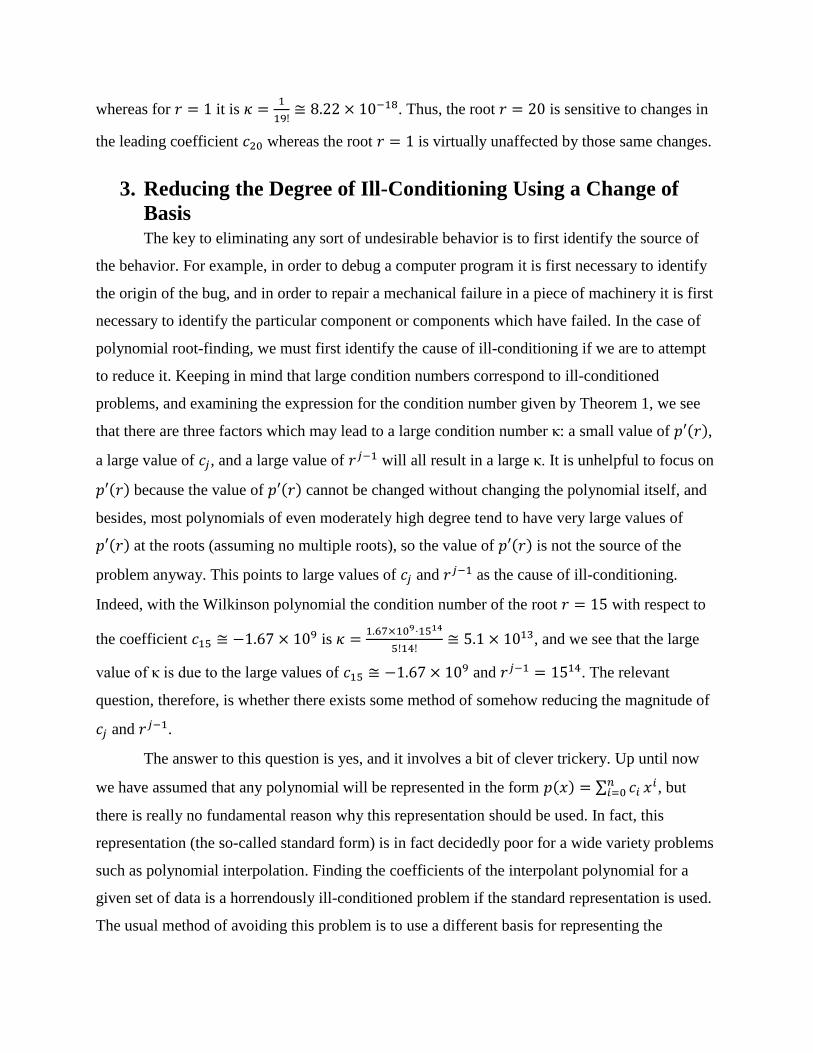
. Thus, the root is sensitive to changes in
the leading coefficient whereas the root is virtually unaffected by those same changes.
3. Reducing the Degree of Ill-Conditioning Using a Change of
Basis The key to eliminating any sort of undesirable behavior is to first identify the source of
the behavior. For example, in order to debug a computer program it is first necessary to identify
the origin of the bug, and in order to repair a mechanical failure in a piece of machinery it is first
necessary to identify the particular component or components which have failed. In the case of
polynomial root-finding, we must first identify the cause of ill-conditioning if we are to attempt
to reduce it. Keeping in mind that large condition numbers correspond to ill-conditioned
problems, and examining the expression for the condition number given by Theorem 1, we see
that there are three factors which may lead to a large condition number κ: a small value of ,
a large value of , and a large value of will all result in a large κ. It is unhelpful to focus on
because the value of cannot be changed without changing the polynomial itself, and
besides, most polynomials of even moderately high degree tend to have very large values of
at the roots (assuming no multiple roots), so the value of is not the source of the
problem anyway. This points to large values of and as the cause of ill-conditioning.
Indeed, with the Wilkinson polynomial the condition number of the root with respect to
the coefficient is
, and we see that the large
value of κ is due to the large values of and . The relevant
question, therefore, is whether there exists some method of somehow reducing the magnitude of
and .
The answer to this question is yes, and it involves a bit of clever trickery. Up until now
we have assumed that any polynomial will be represented in the form , but
there is really no fundamental reason why this representation should be used. In fact, this
representation (the so-called standard form) is in fact decidedly poor for a wide variety problems
such as polynomial interpolation. Finding the coefficients of the interpolant polynomial for a
given set of data is a horrendously ill-conditioned problem if the standard representation is used.
The usual method of avoiding this problem is to use a different basis for representing the
interpolant polynomial; common choices of basis include the Lagrange and Newton bases which
both transform the ill-conditioned problem into a well-conditioned problem. This suggests that it
might be possible to reduce the ill-conditioning of polynomial root-finding using a similar
change of basis. The fundamental idea is that instead of representing a degree n polynomial as
, we may represent it as
, where is a basis
for the vector space of all polynomials of degree n or less. The standard representation is then
a special case of this with . But perhaps a different choice of basis will help alleviate
the problem of sensitivity to small changes in the coefficients. In order to determine exactly what
basis will help with reducing ill-conditioning, we first require an expression for the condition
number of a given root with respect to a given coefficient, using an arbitrary basis. The following
theorem, which is a generalization of Theorem 1 to arbitrary bases, provides such an expression.
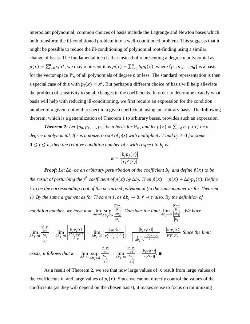
Theorem 2: Let be a basis for , and let be a
degree n polynomial. If r is a nonzero root of p(x) with multiplicity 1 and for some
, then the relative condition number of r with respect to is
Proof: Let be an arbitrary perturbation of the coefficient , and define to be
the result of perturbing the jth
coefficient of by . Then . Define
to be the corresponding root of the perturbed polynomial (in the same manner as for Theorem
1). By the same argument as for Theorem 1, as , also. By the definition of
condition number, we have
. Consider the limit
. We have
Since the limit
exists, it follows that
.
As a result of Theorem 2, we see that now large values of result from large values of
the coefficients and large values of . Since we cannot directly control the values of the
coefficients (as they will depend on the chosen basis), it makes sense to focus on minimizing
; that is, the basis polynomials should have small values near the roots of the original
polynomial. Unfortunately, we do not know the roots because they are precisely what we are
trying to find! Therefore, a possible strategy for attacking the problem might be as follows:
suppose that we have managed to obtain an estimate of the interval in which the roots are
contained; denote this interval by . Then we might choose basis polynomials such that
is small over the entire interval . Assuming that our estimate is sufficiently
accurate, and in particular that all the roots lie inside the interval , the values of the basis
polynomials at the roots of the original polynomial will necessarily be small as well.
It turns out that there exists a particular set of polynomials which work extremely well for
implementing this strategy. These polynomials are the Chebyshev polynomials , and the
special property they have that makes them so useful is that for all n, for .
In addition, the Chebyshev polynomials form an orthogonal set, which makes them relatively
easy to use as a basis for . However, since we must have in order for
to be satisfied, we must make a change of variables to map the original interval onto
. If we let
, then as x ranges over , t ranges over . We may then
express the polynomial as a linear combination of Chebyshev polynomials, find its roots, and
then reverse the change of variables to obtain the roots of the original polynomial. Our procedure
for root-finding is then the following:
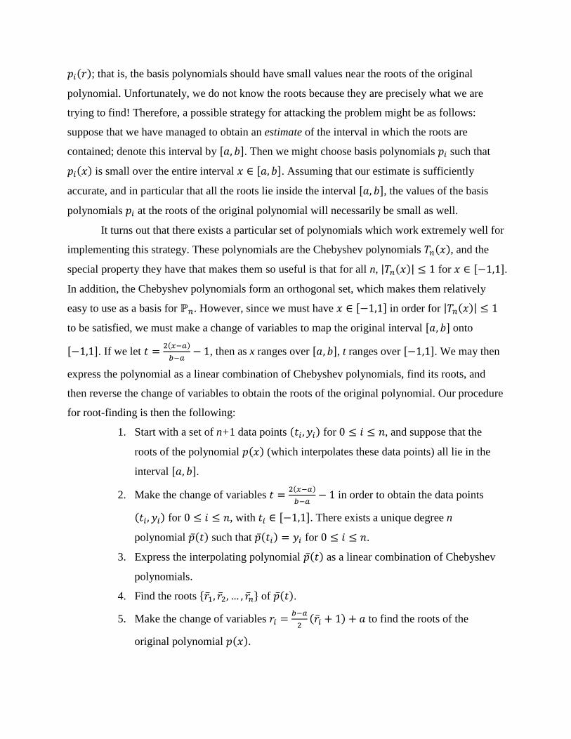
1. Start with a set of n+1 data points for , and suppose that the
roots of the polynomial (which interpolates these data points) all lie in the
interval .
2. Make the change of variables
in order to obtain the data points
for , with . There exists a unique degree n
polynomial such that for .
3. Express the interpolating polynomial as a linear combination of Chebyshev
polynomials.
4. Find the roots of .
5. Make the change of variables
to find the roots of the
original polynomial .
Steps (3) and (4) warrant additional discussion. Several possible procedures can
potentially be used to express a polynomial as a linear combination of Chebyshev polynomials.
One method operates by finding a least-squares approximation to the polynomial , except
that in this case the approximation is exact (at least in theory). Therefore, to find the coefficient
of the ith
Chebyshev polynomial we simply multiply the data points by the Chebyshev
polynomial, divide by , and then integrate over the interval . Unfortunately, since
we only have a set of points on the graph of (enough to uniquely determine it) but do not
have an analytic formula for , a quadrature rule such as the Gauss-Chebyshev quadrature
must be used to evaluate the integral. The disadvantage is that using such a quadrature rule
requires that the data be sampled at certain, specific, pre-determined points, which in many real-
world applications may not always be possible or practical.
Another possible method for expressing the polynomial as a linear combination of
Chebyshev polynomials is by solving the following system of equations: if we have n+1 data
points, so that is degree n, then for , where bj is the coefficient
of the jth
Chebyshev polynomial Tj. In other words, we have where is an
(n+1)-by- (n+1) matrix given by ,
is the vector of coefficients, and
is the vector of measured y-values from the given data. Solving this system then gives
the coefficients bi. However, this approach also has its own issues. If xi and xj are too close
together for some , then the ith
and jth
rows of the matrix will be almost identical, and the
linear system will be ill-conditioned. The result is that there must be a restriction placed on the
minimum distance between x values at which measurements are made. Nevertheless, this
restriction is much looser than the restriction that measurements must be made at certain specific
points (which comes with using Gauss-Chebyshev quadrature to calculate the coefficients).
Therefore, this method is more flexible and would likely be preferred for most real-world
applications. Accordingly, we have decided to use this method in order to obtain experimental
results.
The other noteworthy point is the method for finding the roots of the polynomial .
When finding the roots of a polynomial which is expressed in terms of Chebyshev polynomials,
most advanced methods (such as those based on creating a matrix for which the polynomial is
the characteristic polynomial) are unusable because we are not using the standard form.
Therefore, we can only resort to more elementary methods such as Newton’s method. The
primary issue with Newton’s method is that it can be unpredictable which particular root will be
found, unless the procedure is started sufficiently close to a root. This is problematic if we need
to find one particular root of the polynomial. However, we can still hope that by trying enough
initial conditions, all roots will eventually be found. This issue is beyond the scope of this
research and thus we do not attempt to address it. For the experimental results presented below,
we have taken advantage of the fact that the exact roots are known in order to select a set of
initial conditions which will converge to all the roots of , but it must be kept in mind that
selecting good initial conditions for Newton’s method remains a problem in real-world situations
where at best only a rough estimate of the roots is available.
4. Experimental Results The procedure described in the previous section was used for generating all the results
presented here. In order to obtain a set of data points , the Wilkinson polynomial was
evaluated at 21 equally spaced points in the interval
(and thus the spacing between
successive x values was 1). We used for the interval in which the roots are assumed
to lie.
For the first experiment, after applying the change of variables and expressing the
interpolant polynomial as a linear combination of Chebyshev polynomials, 50
perturbed polynomials were generated by perturbing the coefficients by a random amount up
to 10-10
of the original value (i.e. up to one part in ten billion). This is the same amount which
was previously used to demonstrate the ill-conditioning of the Wilkinson polynomial when
expressed in standard form. The roots of the 50 perturbed polynomials were then found using
Newton’s method. Using Newton’s method for any function requires a means of evaluating the
function and its derivative at any point. This is where another useful property of Chebyshev
polynomials comes into play: they can all be quickly and accurately evaluated at any point using
the formula
(2)
Differentiating both sides gives
(3)
which holds for , with
and
.
Together, equations (2) and (3) provide a means of efficiently evaluating both and
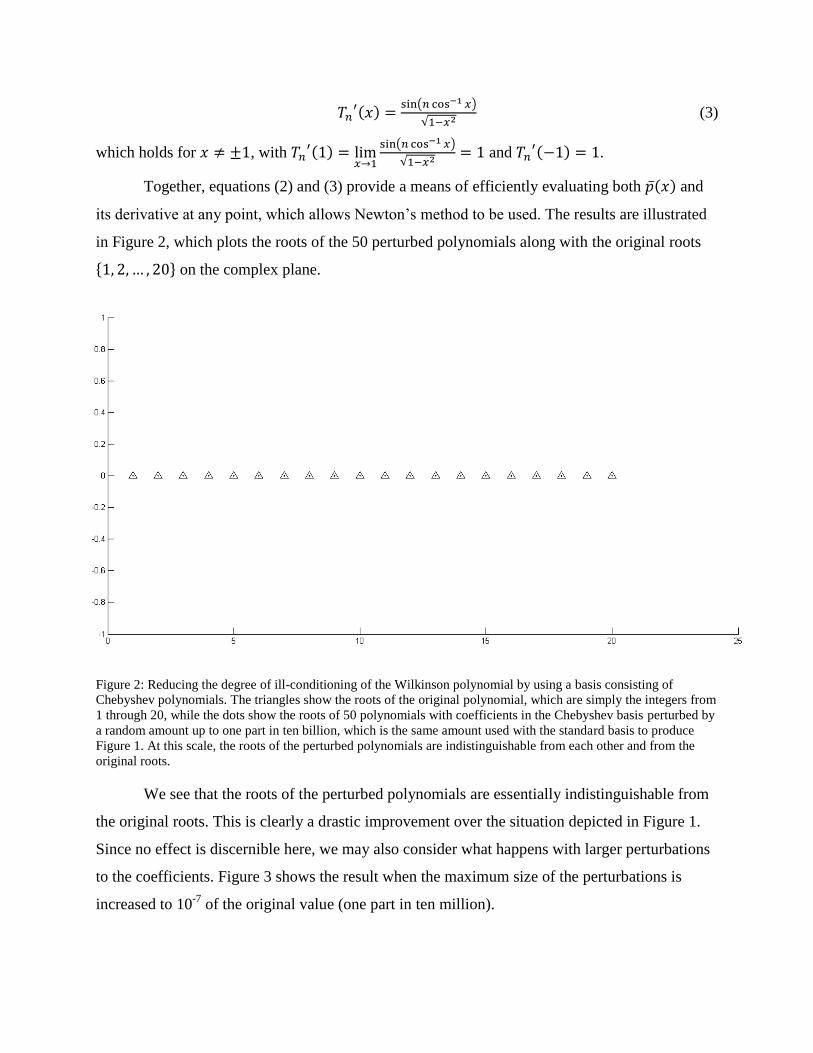
its derivative at any point, which allows Newton’s method to be used. The results are illustrated
in Figure 2, which plots the roots of the 50 perturbed polynomials along with the original roots
on the complex plane.
Figure 2: Reducing the degree of ill-conditioning of the Wilkinson polynomial by using a basis consisting of
Chebyshev polynomials. The triangles show the roots of the original polynomial, which are simply the integers from
1 through 20, while the dots show the roots of 50 polynomials with coefficients in the Chebyshev basis perturbed by
a random amount up to one part in ten billion, which is the same amount used with the standard basis to produce
Figure 1. At this scale, the roots of the perturbed polynomials are indistinguishable from each other and from the
original roots.
We see that the roots of the perturbed polynomials are essentially indistinguishable from
the original roots. This is clearly a drastic improvement over the situation depicted in Figure 1.
Since no effect is discernible here, we may also consider what happens with larger perturbations
to the coefficients. Figure 3 shows the result when the maximum size of the perturbations is
increased to 10-7
of the original value (one part in ten million).
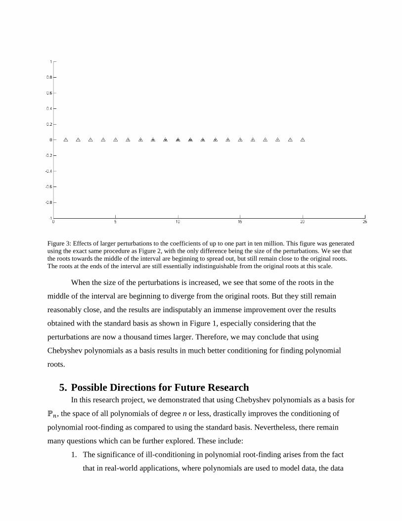
Figure 3: Effects of larger perturbations to the coefficients of up to one part in ten million. This figure was generated
using the exact same procedure as Figure 2, with the only difference being the size of the perturbations. We see that
the roots towards the middle of the interval are beginning to spread out, but still remain close to the original roots.
The roots at the ends of the interval are still essentially indistinguishable from the original roots at this scale.
When the size of the perturbations is increased, we see that some of the roots in the
middle of the interval are beginning to diverge from the original roots. But they still remain
reasonably close, and the results are indisputably an immense improvement over the results
obtained with the standard basis as shown in Figure 1, especially considering that the
perturbations are now a thousand times larger. Therefore, we may conclude that using
Chebyshev polynomials as a basis results in much better conditioning for finding polynomial
roots.
5. Possible Directions for Future Research In this research project, we demonstrated that using Chebyshev polynomials as a basis for
, the space of all polynomials of degree n or less, drastically improves the conditioning of
polynomial root-finding as compared to using the standard basis. Nevertheless, there remain
many questions which can be further explored. These include:
1. The significance of ill-conditioning in polynomial root-finding arises from the fact
that in real-world applications, where polynomials are used to model data, the data
itself will not be exact and so neither will the coefficients. The experimental results
presented here were all obtained by perturbing the coefficients by random amounts
(up to a certain maximum). What would happen if the data itself was perturbed
instead? Note that in real-world situations, the data will have uncertainties in
both the x- and y-values.
2. We used Chebyshev polynomials as an alternative basis because they possessed
certain properties which were likely to reduce the condition number (and thus
improve the conditioning of the problem). However, there is no reason why a
different basis might not work just as well or even better in some situations. It might
even be possible to create up with an adaptive scheme for root-finding where the data
is first analyzed for certain patterns or trends, and then using those patterns a basis is
selected to minimize the ill-conditioning for that particular set of data. This needs to
be further investigated.
3. Using Newton’s method requires that both the function and its derivative can be
accurately evaluated at any point. In this case, the special properties of Chebyshev
polynomials allowed us to do this, but it might not always be possible to find a simple
expression for evaluating other basis polynomials and their derivatives at arbitrary
points. Can the existing linear-algebra based methods for root-finding be generalized
to work for polynomials expressed in terms of an arbitrary basis?
4. In terms of real-world applications, polynomials are often used for more than just
interpolating data. For instance, they can also be used for least-squares
approximations, which in many situations models general trends in the data much
better than a straight interpolation (where the interpolant polynomial passes through
all the data points exactly) does. In these cases, how sensitive are the roots of the
polynomial to changes in the data?
We conclude that while we have demonstrated a method for improving the conditioning
of root-finding in one particular scenario, there are still many questions which need to be
answered in order to use this method for real-world applications. The four points listed above
represent some, but certainly not all, of the directions in which further investigation might be
taken. In general, many of the problems associated with using mathematical theories to model
real-world situations remain wide open.


![On the Schultz polynomial, Modified Schultz polynomial, Hosoya polynomial and Wiener index of circumcoronene series of benzenoid. [7]](https://static.fdokumen.com/doc/165x107/6316d8360f5bd76c2f02aa3c/on-the-schultz-polynomial-modified-schultz-polynomial-hosoya-polynomial-and-wiener.jpg)