A mathematical framework for modelling axon guidance
29
Bulletin of Mathematical Biology (2007) 69: 3–31 DOI 10.1007/s11538-006-9142-4 ORIGINAL ARTICLE A Mathematical Framework for Modeling Axon Guidance Johannes K. Krottje a , Arjen van Ooyen b,∗ a Center for Mathematics and Computer Science, MAS, P.O. Box 94079, 1090 GB Amsterdam, The Netherlands b Department of Experimental Neurophysiology, Center for Neurogenomics and Cognitive Research, Vrije Universiteit Amsterdam, De Boelelaan 1085, 1081 HV Amsterdam, The Netherlands Received: 4 April 2005 / Accepted: 30 June 2005 / Published online: 24 October 2006 C Society for Mathematical Biology 2006 Abstract In this paper, a simulation tool for modeling axon guidance is presented. A mathematical framework in which a wide range of models can been imple- mented has been developed together with efficient numerical algorithms. In our framework, models can be defined that consist of concentration fields of guid- ance molecules in combination with finite-dimensional state vectors. These vec- tors can characterize migrating growth cones, target neurons that release guidance molecules, or other cells that act as sources of membrane-bound or diffusible guid- ance molecules. The underlying mathematical framework is presented as well as the numerical methods to solve them. The potential applications of our simulation tool are illustrated with a number of examples, including a model of topographic mapping. Keywords Axon guidance · Growth cone · Topographic mapping · Simulation · Numerical methods 1. Introduction The proper functioning of the nervous system relies on the formation of cor- rect neuronal connections. During development, neurons project long, thin exten- sions, called axons, which grow out, often over long distances, to form synaptic connections with appropriate target cells. Axons can find their target cells with remarkable precision by using molecular cues in the extracellular space (for re- views, see Tessier-Lavigne and Goodman, 1996; Dickson, 2002; Yamamoto et al., 2003). They steer axons by regulating cytoskeletal dynamics in the growth cone ∗ Corresponding author. E-mail addresses: [email protected] (Johannes K. Krottje), [email protected] (Arjen van Ooyen).
-
Upload
independent -
Category
Documents
-
view
4 -
download
0
Transcript of A mathematical framework for modelling axon guidance
Bulletin of Mathematical Biology (2007) 69: 3–31DOI 10.1007/s11538-006-9142-4
ORIGINAL ARTICLE
A Mathematical Framework for Modeling Axon Guidance
Johannes K. Krottjea, Arjen van Ooyenb,∗
aCenter for Mathematics and Computer Science, MAS, P.O. Box 94079, 1090 GBAmsterdam, The Netherlands
bDepartment of Experimental Neurophysiology, Center for Neurogenomics andCognitive Research, Vrije Universiteit Amsterdam, De Boelelaan 1085, 1081 HVAmsterdam, The Netherlands
Received: 4 April 2005 / Accepted: 30 June 2005 / Published online: 24 October 2006C© Society for Mathematical Biology 2006
Abstract In this paper, a simulation tool for modeling axon guidance is presented.A mathematical framework in which a wide range of models can been imple-mented has been developed together with efficient numerical algorithms. In ourframework, models can be defined that consist of concentration fields of guid-ance molecules in combination with finite-dimensional state vectors. These vec-tors can characterize migrating growth cones, target neurons that release guidancemolecules, or other cells that act as sources of membrane-bound or diffusible guid-ance molecules. The underlying mathematical framework is presented as well asthe numerical methods to solve them. The potential applications of our simulationtool are illustrated with a number of examples, including a model of topographicmapping.
Keywords Axon guidance · Growth cone · Topographic mapping · Simulation ·Numerical methods
1. Introduction
The proper functioning of the nervous system relies on the formation of cor-rect neuronal connections. During development, neurons project long, thin exten-sions, called axons, which grow out, often over long distances, to form synapticconnections with appropriate target cells. Axons can find their target cells withremarkable precision by using molecular cues in the extracellular space (for re-views, see Tessier-Lavigne and Goodman, 1996; Dickson, 2002; Yamamoto et al.,2003). They steer axons by regulating cytoskeletal dynamics in the growth cone
∗Corresponding author.E-mail addresses: [email protected] (Johannes K. Krottje), [email protected](Arjen van Ooyen).

4 Bulletin of Mathematical Biology (2007) 69: 3–31
(Huber et al., 2003), a highly motile and sensitive structure at the tip of a growingaxon. Extracellular cues can either attract or repel growth cones, and can either berelatively fixed or diffuse freely through the extracellular space. Target cells se-crete diffusible attractants and create a gradient of increasing concentration, whichthe growth cone can sense and follow (Goodhill, 1997). Cells that the axons haveto avoid or grow away from produce repellents. By integrating different molecularcues in their environment, growth cones guide axons along the appropriate path-ways and via intermediate targets to their final destination, where they stop grow-ing and form axonal arbors to establish synaptic connections. The responsivenessof growth cones to guidance cues is not static but can change dynamically duringnavigation. Growth cones can undergo consecutive phases of desensitization andresensitization (Ming et al., 2002), and can respond to the same cue in differentways at different points along their journey (Shirasaki et al., 1998; Zou et al., 2000;Shewan et al., 2002). Through modulation of the internal state of the growth cone,attraction can be converted to repulsion and vice versa (Song et al., 1998; Song andPoo, 1999).
Axon guidance is a very active field of research. Several families of moleculeshave been identified and a few general mechanisms can account for many guidancephenomena. The major challenge is now to understand, not only qualitatively butalso quantitatively, how these molecules and mechanisms act in concert to gener-ate the complex patterns of neuronal connections that are found in the nervoussystem.
To address this challenge, experimental work needs to be complemented bymodeling studies. However, unlike for the study of electrical activity in neuronsand neuronal networks (e.g., NEURON; Hines and Carnevale, 1997), there arecurrently no general simulation tools available for axon guidance.
In Hentschel and van Ooyen (1999) a model is presented in which growing ax-ons on a plain are modeled by means of differential equations for the locationsof the growth cones. These equations are coupled to diffusion equations that de-scribe the concentration fields of diffusible chemoattractants and chemorepellents(henceforth referred to as guidance molecules). The system is simplified by us-ing quasi-steady-state approximations for the concentration fields. This approachturns the problem of solving a system consisting of PDEs (partial differential equa-tions) plus ODEs (ordinary differential equations) into a much simpler problemwhere only ODEs have to be solved. This works fine as long as the whole plain isused as a domain for the diffusion equations, but we also want to be able to con-sider more general domains with, for example, areas where diffusion cannot takeplace (“holes”) or with boundaries. Also, Krottje (2003a) showed that in Hentscheland van Ooyen’s approach moving growth cones that secrete diffusible guidancemolecules upon which they respond themselves cause the speed of growth to bestrongly dependent on the diameter of the growth cone (a phenomenon that wascalled self-interaction). The use of a quasi-steady-state approximation will thenresult in heavily distorted dynamics.
Here, we present a general framework for the simulation of axon guidance to-gether with novel numerical methods for carrying out the simulations. The twomajor ingredients of the modeling framework are the concentration fields of the
Bulletin of Mathematical Biology (2007) 69: 3–31 5
guidance molecules and the finite-dimensional state vectors representing thegrowth cones and target neurons. For the latter two, ODEs must be constructedthat describe the interaction with the concentration fields. The dynamics of thefields is described by diffusion equations, where we allow for domains with holesor internal boundaries.
Numerical difficulties arise from small, moving sources for the diffusion equa-tions (see Krottje, 2003a) and from the time integration of a system that is a com-bination of highly nonlinear, non-stiff ODEs and stiff diffusion equations (seeVerwer and Sommeijer, 2001). To circumvent this last difficulty we consider theuse of quasi-steady-state approximations, and we will discuss some criteria on thevalidity of such approximations.
The organization of the paper is as follows. We start with a description of thesimulation framework in Section 2. In Section 3 we will discuss some features ofthe underlying mathematical model and in Section 4 the numerical methods arediscussed. Some simulation examples are given in Section 5. We will finish with adiscussion in Section 6.
2. Simulation framework
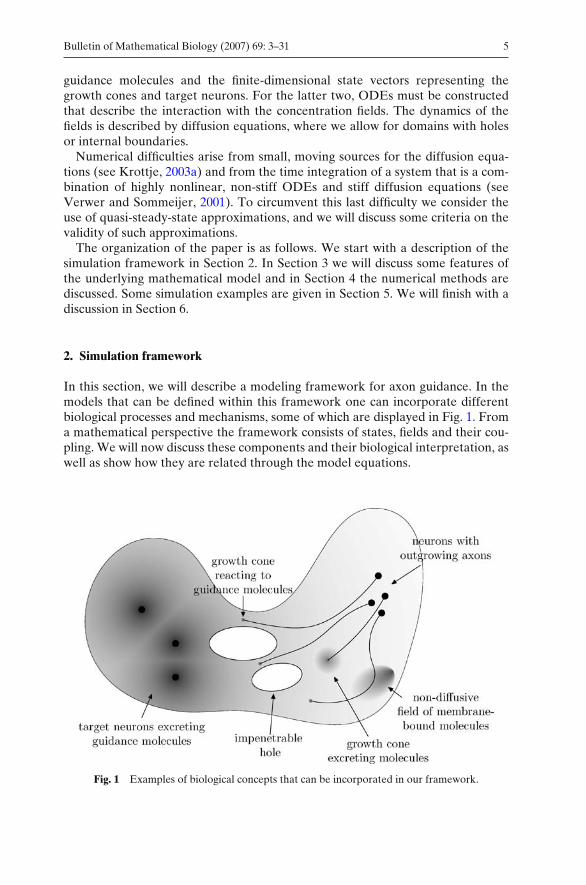
In this section, we will describe a modeling framework for axon guidance. In themodels that can be defined within this framework one can incorporate differentbiological processes and mechanisms, some of which are displayed in Fig. 1. Froma mathematical perspective the framework consists of states, fields and their cou-pling. We will now discuss these components and their biological interpretation, aswell as show how they are related through the model equations.
Fig. 1 Examples of biological concepts that can be incorporated in our framework.
6 Bulletin of Mathematical Biology (2007) 69: 3–31
2.1. States
We define states to be finite-dimensional state vectors that represent objects thatinteract with the concentration fields of guidance molecules. These objects can be,for example, growth cones that move in response to the concentration fields, targetneurons that act as sources of guidance molecules, or locations where artificialinjection of guidance molecules takes place.
We will assume that the first two variables of the state vector will always repre-sent its two-dimensional location, which we will denote by r. Whereas in the modelof Hentschel and van Ooyen a growth cone is completely characterized by its lo-cation r, our description allows for a more general approach in which the state canbe extended with a vector s that further describes the characteristics of the growthcone. Possible characteristics of growth cones and targets that can be modeled withs are as follows:
Sensitivity: Growth cones can respond to different guidance molecules. Their sen-sitivity to a particular molecule may vary over time (Shewan et al., 2002) andcan be influenced by the concentration levels of other guidance molecules aswell as by the level of signaling molecules inside the growth cone (Song andPoo, 1999).
Growth cone geometry: It is known that growth cones can change their size whilemoving through the environment (Rehder and Kater, 1996). The vector scould model how this process depends on the concentration fields, or it couldmodel the way in which changes in growth cone size change the growth cone’ssensitivity or behavior.
Internal state of growth cone: Inside a growth cone biochemical reactions take placethat determine the growth cone’s dynamics (Song et al., 1998; Song and Poo,1999). With s, the concentrations of the different reactants and their effect ongrowth cone dynamics and axon guidance can be modeled.
Production rates: The rate at which target cells produce guidance molecules maydepend on the concentration fields measured at the locations of the targets.The vector s can be used to describe such dependencies. Alternatively, s candescribe production rates that are given explicitly as functions of time.
For the dynamics of the states we allow for two possibilities. In the first one, thestate (r, s) is given explicitly as a function of time t and the different concentrationlevels of guidance molecules ρ j and their gradients ∇ρ j evaluated at position r,
(rs
)=
(Gr(t)
Gs(t, ρ1(r, t),∇ρ1(r, t), . . . , ρM(r, t),∇ρM(r, t))
). (1)
In the second possibility an ODE describes the dynamics of the states,
ddt
(rs
)= G(t, s, ρ1(r, t),∇ρ1(r, t), . . . , ρM(r, t),∇ρM(r, t)). (2)
Bulletin of Mathematical Biology (2007) 69: 3–31 7
The functions Gr , Gs and G are used to model the different biological processesand mechanisms. We will now discuss the fields ρ j ( j = 1, . . . , M).
2.2. Fields
The fields in our framework represent the concentration fields of the guidancemolecules. The dynamics of these fields are determined by diffusion, absorptionand some highly localized sources. With ρ the concentration field, d the diffusioncoefficient, k the absorption coefficient, and Stot a source term, this results in thediffusion equation
∂tρ = d �ρ − kρ + Stot, on � ⊂ R2, n · ∇ρ = 0, on ∂�, (3)
where the domain � may contain several holes (i.e., areas that are impenetrablefor guidance molecules) with piecewise smooth boundaries. Thus, on the boundaryof the domain we will assume that there is no in- or outflow of guidance molecules.A domain is defined by specifying an outer boundary and possibly several internalboundaries. In our framework all boundaries must be given by parameterizationsγi : [0, 1) → �. The parameterizations describe curves. If, for example, an internalboundary is described by a circle, there will be no guidance molecules and there-fore no gradients within the area specified by the circle (see also Example 2 inSection 5).
A number of states is linked to a field. These states determine the total sourcefunction Stot, which is the sum of source functions Si , each of them belonging to asingle state (r, s)i . To further specify the form of the Si , we make use of a transla-tion operator Ty, which can by applied to arbitrary functions η : � → R and whichis defined for y ∈ � by (Tyη)(x) = η(x − y) for all x ∈ �. For the source functionsSi : � → R, we make the assumption that Si = σi (si )Tri S. Here, S is some generalfunction profile and σi (si ) ∈ R denotes the production rate.
We also allow for the possibility of having fields in steady state. A reason toincorporate such fields is that the field dynamics might by significantly faster thanthe dynamics of the growth cones or targets. In this case the fields equation will be
d �ρ − kρ + Stot = 0, on � ⊂ R2, n · ∇ρ = 0, on ∂�, (4)
We will refer to them as quasi-steady-state equations because the source term Stot
may depend on time due to time dependent si and ri .
2.3. Coupling
The coupling between the states and the fields occurs through the arguments ρ j (ri )and ∇ρ j (ri ) in G and the functions σ (si ) in Stot. An example of the coupling isdepicted in Fig. 2, where we have three states and two concentration fields. Herean arrow from one object to another means that the dynamics of the latter objectdepend on the former. For example, the dynamics of state 1 is determined by itselfand the fields A and B, whereas the dynamics of field A depend on states 1 and 2.
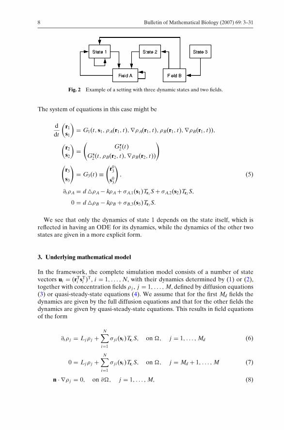
8 Bulletin of Mathematical Biology (2007) 69: 3–31
Fig. 2 Example of a setting with three dynamic states and two fields.
The system of equations in this case might be
ddt
(r1
s1
)= G1(t, s1, ρA(r1, t),∇ρA(r1, t), ρB(r1, t),∇ρB(r1, t)),
(r2
s2
)=
(Gr
2(t)
Gs2(t, ρB(r2, t),∇ρB(r2, t))
)
(r3
s3
)= G3(t) ≡
(r0
3
s03
), (5)
∂tρA = d �ρA − kρA + σA,1(s1)Tr1 S + σA,2(s2)Tr2 S,
0 = d �ρB − kρB + σB,3(s3)Tr3 S.
We see that only the dynamics of state 1 depends on the state itself, which isreflected in having an ODE for its dynamics, while the dynamics of the other twostates are given in a more explicit form.
3. Underlying mathematical model
In the framework, the complete simulation model consists of a number of statevectors ui = (rT
i sTi )T, i = 1, . . . , N, with their dynamics determined by (1) or (2),
together with concentration fields ρ j , j = 1, . . . , M, defined by diffusion equations(3) or quasi-steady-state equations (4). We assume that for the first Md fields thedynamics are given by the full diffusion equations and that for the other fields thedynamics are given by quasi-steady-state equations. This results in field equationsof the form
∂tρ j = Ljρ j +N∑
i=1
σ j i (si )Tri S, on �, j = 1, . . . , Md (6)
0 = Ljρ j +N∑
i=1
σ j i (si )Tri S, on �, j = Md + 1, . . . , M (7)
n · ∇ρ j = 0, on ∂�, j = 1, . . . , M, (8)
Bulletin of Mathematical Biology (2007) 69: 3–31 9
where Lj = dj � − kj . Here, we assume that S : � → R is an L2-function with com-pact support with the property that
∫�
S(x) dx = 1. This means that we can inter-pret the σ j i as the production rate of the source attached to state (r, s)i with respectto field ρ j .
We assume that the dynamics of the first No state vectors are given by ODEs,i.e., equations of the form (2), and that the dynamics of the other vectors are givenexplicitly as a function of time and the fields. When we make use of the notationfor vectors ρ(ri ), ∂xρ(ri ) and ∂yρ(ri ), that are defined by
ρ(ri ) j = ρ j (ri ), ∂xρ(ri ) j = ∂xρ j (ri ), ∂yρ(ri ) j = ∂yρ j (ri ),
this results in
∂t ui = Gi (t, ui , ρ(ri ), ∂xρ(ri ), ∂yρ(ri )), i = 1, . . . , No (9)
(ri
si
)=
(Gr
i (t)
Gsi (t, ρ(ri ), ∂xρ(ri ), ∂yρ(ri ))
), i = No + 1, . . . , N. (10)
In the functions Gi we have to implement the different mechanisms that areinvolved in the behavior of the growth cones and targets when they measure thelevels of particular concentration fields and their gradients. To complete the sys-tem we have to add initial conditions for the states ui and the fields ρ j .
3.1. Moving sources
Our framework also allows for the possibility that guidance molecules are releasedby the growth cones themselves, i.e., we allow for moving sources. Although thebiological evidence for this is not so strong as for the release of guidance moleculesby target cells, it is certainly not implausible. Growth cones secrete various chemi-cals that may operate as chemoattractants and chemorepellents. For example, mi-grating axons are capable of secreting neurotransmitters (Young and Poo, 1983),which have been implicated as chemoattractants (Zheng et al., 1994). The treat-ment of moving sources that respond to guidance molecules they themselves se-crete is mathematically challenging and will be dealt with in the Appendix.
3.2. Quasi-steady-state approximation
When we run a simulation using the whole system (6–10), we should use a timeintegration technique that is suitable for the stiff diffusion equations in combina-tion with the non-stiff ODEs. If the dynamics of all the diffusion equations arefast compared to the state-dynamics, then it is possible to approximate the ρ j ,j = 1, . . . , Md with solutions of the steady-state equations
0 = Ljρ j +N∑
i=1
σ j i (si )Tri S on �, j = 1, . . . , Md. (6′)
10 Bulletin of Mathematical Biology (2007) 69: 3–31
The original dynamical system, which had as its dependent variables the states ui
and the fields ρ j , is now replaced by a dynamical system that has only the ui as itsdependent variables. Although the system at hand is therefore reduced from aninfinite-dimensional to a finite-dimensional system, evaluation of the right-handside still involves solving a infinite-dimensional system. Determination of the val-ues ρ j (ri ) requires solving Eqs. (6′–7). From a numerical perspective the advantageis that we do not need a time integrator that can handle the combination of stiffPDEs and non-stiff ODEs, but we can simply make use of a standard explicit timeintegrator.
To investigate the validity of such an approximation we will consider a diffusionEq. (11) and its steady-state approximation (12)
{∂tρ = d �ρ − kρ + S,
ρ(0, x) = ρ0(x)on R
2 (11)
0 = d �ρ − kρ + S, on R2. (12)
Some implications of using an approximation like (12) for (11) are discussed inKrottje (2003a). There the case of self-interaction is considered, meaning that fora particular field a source is attached to a state and the dynamics of the state isdetermined by the same field. Here, we want to consider some more general crite-ria as to when such a quasi-steady-state approximation might be valid for differentparameter values of the diffusion rate d, the absorption rate k, and the speed asource moves through the domain v.
Hentschel and van Ooyen (1999) used the approximation on the basis of com-paring the time scales of growth and diffusion. Here, however, the absorption pa-rameter plays also a role. To determine criteria that take also k into account wewill follow two approaches. In the first approach we consider the time needed forsetting-up a concentration field. In the second approach we compare the concen-tration profile produced by a point source moving with constant speed with itsquasi-steady-state approximation.
3.3. Field set-up time
To examine how the time for setting up the concentration field depends on d and k,we consider the solution of (11) with S being a point source at the origin, S(x, t) =δ(x), and an initial field ρ = 0 at time t = 0. The solution is rotation symmetric,making it dependent only on the distance to the source r and the time t , ρ(r, t). Inthe Appendix it is shown that it approaches a steady-state solution ρ(r,∞). To seehow fast the field approaches the steady-state field, we consider
c(r, t) = ρ(r,∞) − ρ(r, t)ρ(r,∞)
,
which represents how close the field is to its limit value. For example, a valuec(r, t) = 0.01, means that at time t the field is for 99% set up, at location r . In the
Bulletin of Mathematical Biology (2007) 69: 3–31 11
Appendix we derive
c(r, t) ∼ 1
2K0
(r√
kd
) e−kt
kt, (13)
where K0 is a modified Bessel function of the Second Kind (Abramowitz andStegun, 1964). This can be used to get an indication of the time scale of the fielddynamics. Such an indicator is important if we want to work with fields in whichthe sources do not move through the domain. In case of moving sources, one mightwonder how the speed of a source influences the produced field. To this end weexamine the solution of (11) with a point source that moves with constant speed.
3.4. Field produced by moving source
Consider Eq. (11) with a point source that moves with constant speed v along thex-axis in positive direction, i.e., S(x, t) = δ(x − vt), with v = (v, 0)T. In the Ap-pendix it is shown that we get a stable constant profile solution that moves alsowith constant speed v.
Here, we want to compare how close the quasi steady-state-approximation so-lution ρs is to this moving profile solution ρp. It turns out that in the vicinity of thesource the moving profile is smaller than the steady-state-approximation, and onapproaching the location of the source they tend to become equal. In the Appendixit is derived that the area around the source for which the difference between thequasi-steady-state approximation ρs and the moving profile solution ρp is smallerthan some threshold, is circular in first-order approximation in the distance to thesource
r � 2e−γE
√dk
(1 + v2
4dk
) 12(γ−1)
=⇒ γ �ρp
ρs≤ 1. (14)
If we choose γ = 0.99, we get an indication of the radius r of the region aroundthe source where the difference between the moving profile and the quasi-steady-state solution is less than about 1%, given the values of the diffusion rate d, ab-sorption rate k and moving speed v.
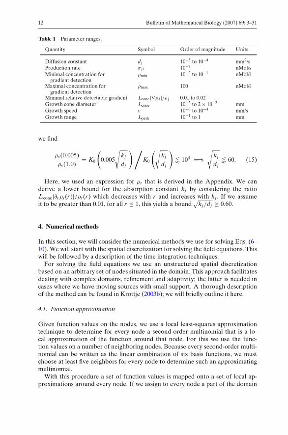
3.5. Typical parameter ranges
Based on in vitro data of chick spinal sensory axons, chick retinal axons and leuko-cyte chemotaxis, Goodhill (1998) gives some estimates for the ranges of some rel-evant parameters. Table 1 shows a list with parameter ranges. The ratio of themaximal and minimal concentration for gradient detection ρmax/ρmin can be usedtogether with the diffusion constant d to find an upper bound on the possible valuesof the absorption parameter kj . Assume that the ratio ρmax/ρmin is 100/10−2 = 104
and that we have a point source located at the origin that produces the steady-state field ρs(r). Then using the assumptions that the maximal distance over whicha cone can be guided Lpath is 1 mm and the growth cone radius equals 0.005 mm,
12 Bulletin of Mathematical Biology (2007) 69: 3–31
Table 1 Parameter ranges.
Quantity Symbol Order of magnitude Units
Diffusion constant dj 10−5 to 10−4 mm2/sProduction rate σ j i 10−7 nMol/sMinimal concentration for ρmin 10−2 to 10−1 nMol/l
gradient detectionMaximal concentration for ρmax 100 nMol/l
gradient detectionMinimal relative detectable gradient Lcone|∇ρ j |/ρ j 0.01 to 0.02Growth cone diameter Lcone 10−2 to 2 × 10⁻² mmGrowth speed v 10−6 to 10−4 mm/sGrowth range Lpath 10−1 to 1 mm
we find
ρs(0.005)ρs(1.0)
= K0
(0.005
√kj
dj
) /K0
(√kj
dj
)� 104 =⇒
√kj
dj� 60. (15)
Here, we used an expression for ρs that is derived in the Appendix. We canderive a lower bound for the absorption constant kj by considering the ratioLcone|∂rρs(r)|/ρs(r) which decreases with r and increases with kj . If we assumeit to be greater than 0.01, for all r ≤ 1, this yields a bound
√kj/dj ≥ 0.60.
4. Numerical methods
In this section, we will consider the numerical methods we use for solving Eqs. (6–10). We will start with the spatial discretization for solving the field equations. Thiswill be followed by a description of the time integration techniques.
For solving the field equations we use an unstructured spatial discretizationbased on an arbitrary set of nodes situated in the domain. This approach facilitatesdealing with complex domains, refinement and adaptivity; the latter is needed incases where we have moving sources with small support. A thorough descriptionof the method can be found in Krottje (2003b); we will briefly outline it here.
4.1. Function approximation
Given function values on the nodes, we use a local least-squares approximationtechnique to determine for every node a second-order multinomial that is a lo-cal approximation of the function around that node. For this we use the func-tion values on a number of neighboring nodes. Because every second-order multi-nomial can be written as the linear combination of six basis functions, we mustchoose at least five neighbors for every node to determine such an approximatingmultinomial.
With this procedure a set of function values is mapped onto a set of local ap-proximations around every node. If we assign to every node a part of the domain
Bulletin of Mathematical Biology (2007) 69: 3–31 13
for which we assume the local approximation to be valid, such that the whole do-main is covered, this results in a global approximation. For a given set of functionvalues in a vector w ∈ R
N, we denote the global approximation by F(w) ∈ L1(�),where L1(�) is the space of integrable real functions defined on � ⊂ R
2.
4.2. Voronoi diagrams
For choosing neighboring nodes of nodes, as well as for assigning parts of the do-main to the nodes, we use the Voronoi diagram (Fortune, 1987). It assigns to everynode a Voronoi cell, which is the set of points closer to the node than to everyother node, hence dividing the domain and at the same time creating neighbors ina natural way.
Because a Voronoi diagram extends to all of R2, we will truncate it by connecting
the nodes on the boundary by straight lines, resulting in a bounded diagram. Fromnow on all our diagrams will be truncated ones, but we will still refer to them asVoronoi diagrams. Determination of such a diagram can be done in O (N log(N))operations, where N is the number of nodes (de Berg et al., 2000). We store thediagram in a totally disconnected edge list (de Berg et al., 2000), so that searchingneighboring nodes for every node becomes a process of O (N) operations.
4.3. Variational problem
Solving equations of the form (7) can be done by solving the variational problemof minimizing A(w,w) − L(S, w) over w ∈ H1 (Atkinson and Han, 2001; Krottje,2003b), where
A(v,w) =∫
�
12 d ∇v · ∇w + 1
2κvw dx, (16)
L(S, w) =∫
�
Sw dx. (17)
A direct discretization of this problem is to minimize A(F(w), F(w)) −L(F(S), F(w)), over all w ∈ R
N, where S ∈ RN is the vector of S-values at the
nodes. It can be shown (Krottje, 2003b) that sparse matrices A and L exist suchthat 1
2 wT Aw = A(F(w), F(w)) and ST Lw = L(F(S), F(w)). If A is non-singularthe discrete problem has a unique solution w = A−1S. With the algorithm for find-ing the Voronoi diagram comes a lexicographical ordering of the nodes that willgive the sparse matrices a band structure, which is advantageous when solving thesystem directly using an LU-decomposition.
Convergence tests show that the solution is second-order convergent in the L2-norm, with respect to the maximum distance between neighboring nodes (Krottje,2003b).
4.4. Choosing nodes
To distribute nodes appropriately over a domain we make use of Lloyd’s algo-rithm (Du et al., 1999). This algorithm is based upon the determination of Voronoi
14 Bulletin of Mathematical Biology (2007) 69: 3–31
diagrams and the process of shifting nodes to centroids of Voronoi cells. An alter-nating sequence of these two operations distributes the nodes equally over thedomain, in the sense that distances between neighbors will tend to become equalthroughout the diagram.
To achieve refinement at certain points, we use a variation of Lloyd’s algorithm.Here, after shifting the nodes to their centroids, an extra shift in the directionof neighboring nodes is added. To determine for a particular node which of itsneighbors are attracting this node, all nodes are given an integer type. Nodes willthen be attracted to the neighbors with higher type than their own type.
To get refinement around a certain point in the domain, a node is fixed at thatpoint and several rings of decreasing node type are defined around it. The ex-tended Lloyd’s algorithm then moves nodes around, which results in a refinementaround the fixed node.
In contrast to methods where refinement is based on local error estimation, hererefinement takes place around the source locations. This is done because we knowin advance that only at those locations, and possibly at the boundary, refinementis required for optimal accuracy. Doing it in this way instead of using an errorestimation process will speed up the refinement process.
Having discussed the spatial discretization method we will now focus on the timeintegration. We will consider three different cases that can be distinguished by thefield dynamics in the model.
4.5. Time integration with static fields
We first consider the case with static fields only. In this case we only have ODEswhich need the solutions of the fields for the evaluation of their right-hand sides.These fields are determined at the start of the simulation by solving the ellipticequations, giving the approximations to the field solutions ρ1, . . . , ρM. After thisthe growth cone dynamics can be solved using a standard explicit ODE solver.
For the fields to be static we need a number of static states that make up thesources of the fields. Let us assume that of all the states only the last Ns are static,i.e., (ri , si ) = constant, and that the rest of the states do not influence the fielddynamics. Thus, we must have
σ j i ≡ 0, for all
{j = 1, . . . , M, (all fields)
i = 1, . . . , N − Ns (all dynamic states).(18)
Then given the Ns static positions ri , i > N − Ns , we have to solve
si = Gsi (ρ(ri ), ∂xρ(ri ), ∂yρ(ri )), i = N − Ns + 1, . . . , N. (19)
Ljρ j +N∑
i=N−Ns+1
σ j i (si )Tri S = 0, on �, (20)
n · ∇ρ j = 0, on ∂�, j = 1, . . . , M.
Bulletin of Mathematical Biology (2007) 69: 3–31 15
This system can be solved by solving first the field Eq. (20). Using the inverseoperators of Lj with respect to the boundary conditions, we get
ρ j = −N∑
i=N−Ns+1
σ j i (si )L−1j Tri S, on �. (21)
When combined with Eq. (19), evaluation of these field solutions and their gradi-ents in the given ri , results in a closed algebraic system with respect to si , ρ j (ri ),∂xρ j (ri ) and ∂yρ j (ri ). We will assume that this nonlinear system can be solved,although the solvability depends on the ri and the functions σ j i .
Therefore, to solve numerically the fields ρ j we first have to solve numericallythe fields L−1
j Tri S, using the spatial discretization above. After evaluation of thesefields (i.e., their numerical approximations) and their derivatives in all locations ri ,the algebraic system can be built by substituting (21) into (19). We can solve thissystem by using, for example, Newton iterations and use the si to determine thesolutions ρ j .
Once the fields and static states (i > N − Ns) are solved we can start solving thenon-static states from the equations
∂t ui = Gi (t, ui , ρ(ri ), ∂xρ(ri ), ∂yρ(ri )), i = 1, . . . , No (22)
(ri
si
)=
(Gr
i (t)
Gsi
(t, ρ(ri ), ∂xρ(ri ), ∂yρ(ri )
))
, i = No + 1, . . . , N − Ns . (23)
where No was defined above Eq. (9). For solving the ODEs we choose an explicitintegration scheme because the ODEs are non-stiff (and nonlinear). We will usethe classical fourth-order RK (see, for example Hundsdorfer and Verwer, 2003)for this. Note that for the function evaluations we have to determine local approx-imations of the fields and their gradients. A slight difficulty arises here because thelocal least-squares approximations are discontinuous from one Voronoi cell to an-other. Therefore, if the integration process crosses the edge of a cell during a timestep, there will be loss of order with respect to the size of the time step. To preventthis we make sure that during a time step we use for every state only one local fieldapproximation for all function evaluations used in the scheme. Because the localfield approximation is a multinomial the order of the scheme will be retained.
4.6. Quasi-steady-state approximation
When using quasi-steady-state approximations for the fields, the system we haveto solve is
∂t ui = Gi (t, ui , ρ(ri ), ∂xρ(ri ), ∂yρ(ri )), i = 1, . . . , No (24)
(ri
si
)=
(Gr
i (t)
Gsi (t, ρ(ri ), ∂xρ(ri ), ∂yρ(ri ))
), i = No + 1, . . . , N, (25)
Ljρ j + ∑Ni=1 σ j i (si )Tri S = 0, on �,
n · ∇ρ j = 0, on ∂�,
}j = 1, . . . , M. (26)
16 Bulletin of Mathematical Biology (2007) 69: 3–31
Here we use, as in the previous case, an explicit time integrator for the ODEs in(24). To evaluate the right-hand side of the equations we need to solve the fields ρ j
for given values of (ri , si )n, i = 1, . . . , No, and tn, where n denotes the time level. Tofind these we have to determine the fields again by solving a non-linear algebraicsystem as is done in the case with static fields. Here, the system will have as itsunknowns the ρ j (ri ), ∂xρ j (ri ) and ∂yρ j (ri ) for all combinations of fields ρ j andstates ri , together with all si , for i > No.
In contrast to the case with static fields, every function evaluation in the right-hand side of (24) requires solving Eq. (26) and evaluation of the resulting solutionfields and their gradients. Also, because the source terms in (26) depend on thestates ui , it may be necessary to redefine the nodes used to solve the field equations.Therefore, solving such a system is computationally much more expensive thansolving a system with static fields only.
4.7. Full system
Solving the full system, i.e., Eqs. (6–10), requires a numerical method that can dealwith both the nonlinear, non-stiff ODEs and the stiff diffusion equations. Verwerand Sommeijer (2001) use for a system similar to the combination of (6) and (9)the RKC method, which is explicit and can deal with moderately stiff systems dueto a long narrow stability region around the negative real axis. Lastdrager (2002)used a Rosenbrock method with approximate Jacobians for the same system sothat effectively the field equations are integrated implicitly and the state equationsexplicitly, as with IMEX (IMplicit-EXplicit) methods (Hundsdorfer and Verwer,2003).
We use an Runge–Kutta IMEX scheme, in particular an IMEX-midpointscheme, which can be seen as a combination of an implicit and an explicit mid-point step. For a system x = f1(t, x) + f2(t, x) it is given by
xs = xn + 12τ f1
(tn + 1
2τ, xs
)+ 1
2τ f2(tn, xn),
(27)
xn+1 = 2xs − xn + τ
(f2
(tn + 1
2τ, xs
)− f2(tn, xn)
),
where the s in xs refers to the intermediate stage. For our system the part f1,which is treated implicitly, contains the linear operators Li from Eq. (6), whilethe explicit part f2 contains the source terms of Eq. (6) and the functions Gi fromEq. (9). This is a second-order time integration method and the implicit part, i.e.,the implicit midpoint method, is A-stable. Also, using this scheme for the systemsat hand never revealed any stability problems.
In the next section, we will show some example models. Although our frame-work can deal with non-static fields (as discussed earlier), in these examples wewill consider only cases in which the fields are static.
Bulletin of Mathematical Biology (2007) 69: 3–31 17
5. Simulation examples
In this section, we will discuss simulations of some example models. We want tostress that the models used here are still simple and only serve to show the differentpossibilities of our framework. To model the growth cones and the sources of theguidance molecules, such as target cells, we have to choose state vectors (ri , si )that characterize these objects and accompanying functions G that describe thedynamics through Eqs. (1) and (2).
5.1. Growth cone model
As a first example of a growth cone model we consider growth cones characterizedby three-dimensional state vectors. To the position ri = (x, y) we add a variablerepresenting the orientation angle si = φ ∈ [0, 2π) of the growth cone. This givesour model growth cone a growth direction, which it has to adjust in order to steer.It gives the opportunity to build in some kind of ‘stiffness’, the inability to undergoinstant changes in growth direction.
In order to describe the dynamics of the growth direction we need to define adifferential equation. We will assume that the growth speed is constant, given asv, and that the cone grows with this speed in the direction given by the orientationangle φ, i.e., ri = (v cos(φ), v sin(φ)). For the dynamics of φ, we assume that it iscontinuously compared with some ideal direction φg , which we will assume to be alinear combination of the sensed gradients of the fields ρ j evaluated at location ri ,
φg = arg
⎛⎝ N∑
j=1
λ j (ρ(ri ))∇ρ j (ri )
⎞⎠ , (28)
with ‘arg’ the function that returns the angle between the argument and the pos-itive x-axis. Here, the real functions λ j determine the sensitivity to each of thefields. A positive λ j will cause the cone to be attracted by the field ρ j , while anegative λ j causes repulsion.
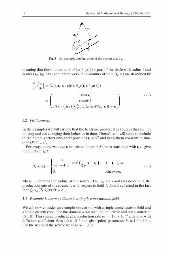
To formulate an ODE for φ that depends on the value of φg , we use the map-ping φ → (sin(φ), cos(φ)) to view the growth directions as two-dimensional unitvectors, z and zg , respectively. The ideal direction zg can be split in a part parallelto the growth direction z and a part that is perpendicular to it, zg = z‖ + z⊥. Anillustration of this is shown in Fig. 3. We assume that z = (v/ )z⊥. Returning toangles φ and φg this results in φ = v/ sin(φg − φ).
Here, the parameter is a measure for the smallest circle the growth conecan make while turning. This latter fact can be understood by realizing that themaximal value of φ is v/ . If we consider a solution where φ is maximal we get,with r = (x, y),
ddt
(xy
)=
(φ cos(φ)
φ sin(φ)
)=⇒
(xy
)=
( sin(φ(t)) + x0
− cos(φ(t)) + y0
),
18 Bulletin of Mathematical Biology (2007) 69: 3–31
Fig. 3 An example configuration of the vectors z and zg .
meaning that the solution path of (x(t), y(t)) is part of the circle with radius andcenter (x0, y0). Using the framework the dynamics of state (ri , si ) are described by
ddt
(ri
si
)= Gi (t, ri , si , ρ(ri ), ∂xρ(ri ), ∂yρ(ri ))
=
⎛⎜⎝
v cos(si )
v sin(si )
v/ sin(
arg( ∑N
j=1 λ j (ρ(ri ))∇ρ j (ri )) − si
)
⎞⎟⎠ .
(29)
5.2. Field sources
In the examples we will assume that the fields are produced by sources that are notmoving and not changing their behavior in time. Therefore, it will serve to includein their state vectors only their positions ri ∈ R
2 and keep them constant in timeri = Gr
i (t) ≡ r0i .
For every source we take a bell shape function S that is translated with ri to givethe function Tri S,
(Tri S)(x) =
⎧⎪⎨⎪⎩
2π
(π2 − 4)w2cos2
( π
2w|x − ri |
), |x − ri | ≤ w,
0, otherwise,(30)
where w denotes the radius of the source. The σ j i are constants describing theproduction rate of the source i , with respect to field j . This is reflected in the factthat
∫�
σ j i (Tri S)(x) dx = σ j i .
5.3. Example 1. Axon guidance in a simple concentration field
We will now consider an example simulation, with a single concentration field anda single growth cone. For the domain � we take the unit circle and put a source at(0.5, 0). This source produces at a production rate σ11 = 1.0 × 10⁻⁴ a field ρ1 withdiffusion coefficient d1 = 1.0 × 10⁻⁴ and absorption parameter k1 = 1.0 × 10⁻⁴.For the width of the source we take w = 0.02.
Bulletin of Mathematical Biology (2007) 69: 3–31 19
The growth cone is modeled by using system (29) with the functions λ1 setto λ1 ≡ 1, which means that φg = arg ∇ρ1. Further we use the parameter valuesv = 1.0 × 10⁻⁵ and = 0.02.
Thus, the total system we have to solve becomes
d1 �ρ1(x) − k1ρ1(x) + σ11Tr1 S(x) = 0, ∀x ∈ �,
n(x) · ∇ρ1(x) = 0, ∀x ∈ ∂�,
r1 = (0.5, 0)
ddt
(r2
s2
)=
⎛⎜⎝
v cos(s2)
v sin(s2)
v/ sin (arg (∇ρ1(r2)) − s2)
⎞⎟⎠
r2(0) = (x0, y0),s2(0) = φ0,
v = 1.0 × 10⁻⁵,
= 0.02
(31)
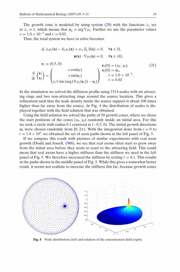
In the simulation we solved the diffusion profile using 1514 nodes with six attract-ing rings and two non-attracting rings around the source location. This gives arefinement such that the node density inside the source support is about 100 timeshigher than far away from the source. In Fig. 4 the distribution of nodes is dis-played together with the field solution that was obtained.
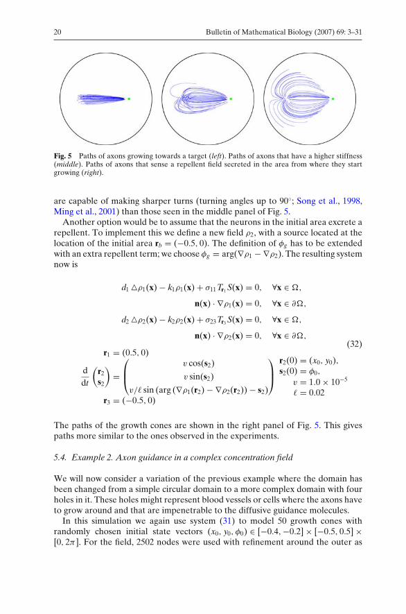
Using the field solution we solved the paths of 50 growth cones, where we chosethe start positions of the cones (x0, y0) randomly inside an initial area. For thiswe took a circle with radius 0.1 centered at (−0.5, 0). The initial growth directionsφ0 were chosen randomly from [0, 2π). With the integration done from t = 0 tot = 1.0 × 10⁵, we obtained the set of axon paths shown in the left panel of Fig. 5.
If we compare this result with pictures of similar experiments with real axongrowth (Dodd and Jessell, 1988), we see that real axons often start to grow awayfrom the initial area before they seem to react to the attracting field. This couldmean that real axons have a higher stiffness than the stiffness we used in the leftpanel of Fig. 5. We therefore increased the stiffness by setting = 0.1. This resultsin the paths shown in the middle panel of Fig. 5. While this gives a somewhat betterresult, it seems not realistic to increase the stiffness this far, because growth cones
Fig. 4 Node distribution (left) and solution of the concentration field (right).
20 Bulletin of Mathematical Biology (2007) 69: 3–31
Fig. 5 Paths of axons growing towards a target (left). Paths of axons that have a higher stiffness(middle). Paths of axons that sense a repellent field secreted in the area from where they startgrowing (right).
are capable of making sharper turns (turning angles up to 90◦; Song et al., 1998,Ming et al., 2001) than those seen in the middle panel of Fig. 5.
Another option would be to assume that the neurons in the initial area excrete arepellent. To implement this we define a new field ρ2, with a source located at thelocation of the initial area rb = (−0.5, 0). The definition of φg has to be extendedwith an extra repellent term; we choose φg = arg(∇ρ1 − ∇ρ2). The resulting systemnow is
d1 �ρ1(x) − k1ρ1(x) + σ11Tr1 S(x) = 0, ∀x ∈ �,
n(x) · ∇ρ1(x) = 0, ∀x ∈ ∂�,
d2 �ρ2(x) − k2ρ2(x) + σ23Tr3 S(x) = 0, ∀x ∈ �,
n(x) · ∇ρ2(x) = 0, ∀x ∈ ∂�,
r1 = (0.5, 0)
ddt
(r2
s2
)=
⎛⎜⎝
v cos(s2)
v sin(s2)
v/ sin (arg (∇ρ1(r2) − ∇ρ2(r2)) − s2)
⎞⎟⎠
r3 = (−0.5, 0)
r2(0) = (x0, y0),s2(0) = φ0,
v = 1.0 × 10−5
= 0.02
(32)
The paths of the growth cones are shown in the right panel of Fig. 5. This givespaths more similar to the ones observed in the experiments.
5.4. Example 2. Axon guidance in a complex concentration field
We will now consider a variation of the previous example where the domain hasbeen changed from a simple circular domain to a more complex domain with fourholes in it. These holes might represent blood vessels or cells where the axons haveto grow around and that are impenetrable to the diffusive guidance molecules.
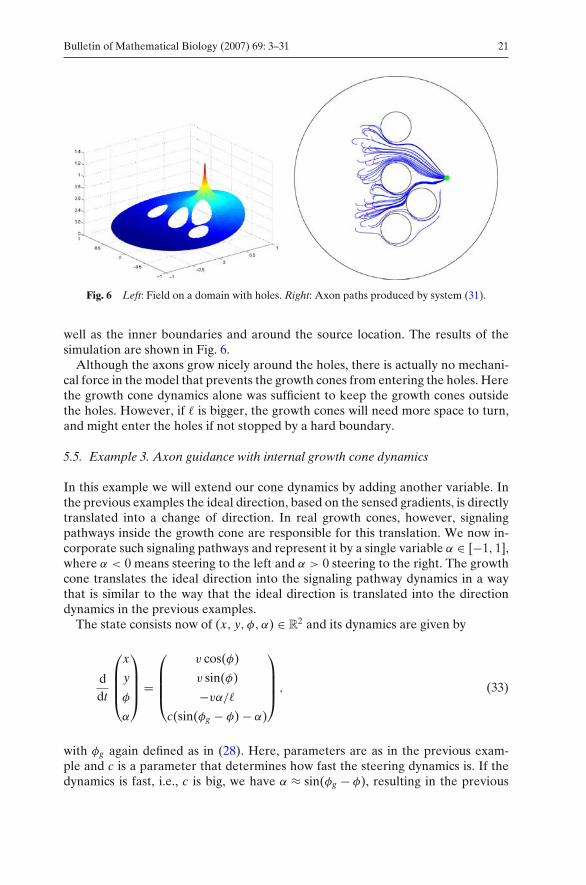
In this simulation we again use system (31) to model 50 growth cones withrandomly chosen initial state vectors (x0, y0, φ0) ∈ [−0.4,−0.2] × [−0.5, 0.5] ×[0, 2π]. For the field, 2502 nodes were used with refinement around the outer as
Bulletin of Mathematical Biology (2007) 69: 3–31 21
Fig. 6 Left: Field on a domain with holes. Right: Axon paths produced by system (31).
well as the inner boundaries and around the source location. The results of thesimulation are shown in Fig. 6.
Although the axons grow nicely around the holes, there is actually no mechani-cal force in the model that prevents the growth cones from entering the holes. Herethe growth cone dynamics alone was sufficient to keep the growth cones outsidethe holes. However, if is bigger, the growth cones will need more space to turn,and might enter the holes if not stopped by a hard boundary.
5.5. Example 3. Axon guidance with internal growth cone dynamics
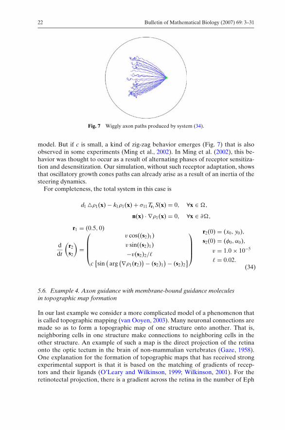
In this example we will extend our cone dynamics by adding another variable. Inthe previous examples the ideal direction, based on the sensed gradients, is directlytranslated into a change of direction. In real growth cones, however, signalingpathways inside the growth cone are responsible for this translation. We now in-corporate such signaling pathways and represent it by a single variable α ∈ [−1, 1],where α < 0 means steering to the left and α > 0 steering to the right. The growthcone translates the ideal direction into the signaling pathway dynamics in a waythat is similar to the way that the ideal direction is translated into the directiondynamics in the previous examples.
The state consists now of (x, y, φ, α) ∈ R2 and its dynamics are given by
ddt
⎛⎜⎜⎜⎝
x
y
φ
α
⎞⎟⎟⎟⎠ =
⎛⎜⎜⎜⎝
v cos(φ)
v sin(φ)
−vα/
c(sin(φg − φ) − α)
⎞⎟⎟⎟⎠ , (33)
with φg again defined as in (28). Here, parameters are as in the previous exam-ple and c is a parameter that determines how fast the steering dynamics is. If thedynamics is fast, i.e., c is big, we have α ≈ sin(φg − φ), resulting in the previous
22 Bulletin of Mathematical Biology (2007) 69: 3–31
Fig. 7 Wiggly axon paths produced by system (34).
model. But if c is small, a kind of zig-zag behavior emerges (Fig. 7) that is alsoobserved in some experiments (Ming et al., 2002). In Ming et al. (2002), this be-havior was thought to occur as a result of alternating phases of receptor sensitiza-tion and desensitization. Our simulation, without such receptor adaptation, showsthat oscillatory growth cones paths can already arise as a result of an inertia of thesteering dynamics.
For completeness, the total system in this case is
d1 �ρ1(x) − k1ρ1(x) + σ11Tr1 S(x) = 0, ∀x ∈ �,
n(x) · ∇ρ1(x) = 0, ∀x ∈ ∂�,
r1 = (0.5, 0)
ddt
(r2
s2
)=
⎛⎜⎜⎜⎝
v cos((s2)1)
v sin((s2)1)
−v(s2)2/
c{sin
(arg
(∇ρ1(r2)) − (s2)1
) − (s2)2}
⎞⎟⎟⎟⎠
r2(0) = (x0, y0),
s2(0) = (φ0, α0),
v = 1.0 × 10−5
= 0.02.
(34)
5.6. Example 4. Axon guidance with membrane-bound guidance moleculesin topographic map formation
In our last example we consider a more complicated model of a phenomenon thatis called topographic mapping (van Ooyen, 2003). Many neuronal connections aremade so as to form a topographic map of one structure onto another. That is,neighboring cells in one structure make connections to neighboring cells in theother structure. An example of such a map is the direct projection of the retinaonto the optic tectum in the brain of non-mammalian vertebrates (Gaze, 1958).One explanation for the formation of topographic maps that has received strongexperimental support is that it is based on the matching of gradients of recep-tors and their ligands (O’Leary and Wilkinson, 1999; Wilkinson, 2001). For theretinotectal projection, there is a gradient across the retina in the number of Eph
Bulletin of Mathematical Biology (2007) 69: 3–31 23
receptors on the growth cones of the retinal neurons. A similar but oppositegradient is found across the tectum in the number of membrane-bound ephrinmolecules (the ligands for Eph receptors) on the tectal neurons. Axons grow outso that growth cones with a low number of receptors come to connect to tectal cellswith a high number of ligand molecules, and vice versa.
A simple model for this phenomenon is the following (see also Honda et al.,1998). We use essentially model (29), but we extend it with two extra variables, βx
and βy, that represent the levels of two kinds of receptors. These βx and βy remainconstant during growth and vary with respect to the initial location r0 = (x0, y0).We take for these
βx = exp(1.39x0 + 1.18) and βy = exp (1.39y0 + 0.35). (35)
We will assume that there are five fields of which three are diffusive fields andtwo are fields of membrane-bound ligands. Fields ρ1, ρ2 and ρ3 are producedby guidance cells located at r1 = (−0.1, 0), r2 = (0.85, 0) and r3 = (0.3, 0.85), re-spectively. We use the same diffusion rate d = 1.0 × 10⁻⁴ and the absorption ratek = 1.0 × 10⁻⁴ as in the previous examples. The two fields of membrane boundligands ρ4 and ρ5 are described by explicit functions that are given by
ρ4(x, y) = exp(−1.39x + 0.21) and ρ5(x, y) = exp(−1.39y + 0.14). (36)
We will assume that the dynamics of the growth cones occurs in two phases. Inthe first phase the growth cones are attracted by field ρ1 and they grow toward theguidance cell located at r0. Once they have reached the guidance cell, which wewill formalize by (Tr1 S)(r) > 0, they switch their behavior and phase two will start.The dynamics of the growth cones during the first phase are given by
ddt
⎛⎜⎜⎜⎜⎝
xyφ
βx
βy
⎞⎟⎟⎟⎟⎠ =
⎛⎜⎜⎜⎜⎜⎜⎝
v cos(φ)
v sin(φ)
v/ sin(φg − φ)
0
0
⎞⎟⎟⎟⎟⎟⎟⎠
, with φg = arg(∇ρ1(r)
). (37)
For the dynamics of the growth cones in phase two we need assumptions onthe influence of the receptors and ligands on the growth. The basic assumptionis the following. For each direction, i.e., x- or y-direction, we have a couple ofreceptor and ligand pairs. For growth in either of these directions it is needed thatthe concentration of the ligand in the neighborhood of the cone is above a certainlevel, which is determined by the receptor density on the growth cone. We willassume that growth in the x-direction is determined by the product cx = βxρ4(r)(and similar cy = βyρ5(r) for the y-direction) A cx � 1 means strong inhibitionof growth in the x-direction and cx � 1 means no inhibition. The dynamics is the
24 Bulletin of Mathematical Biology (2007) 69: 3–31
same as in the first phase, but now with
φg = arg(Sgm20(cx)∇ρ2(r) + Sgm20(cy)∇ρ3(r)). (38)
Here the function Sgmn is defined by Sgmn(x) = xn/(1 + xn). Finally, we will as-sume that the growth is completely inhibited if both cx < 0.8 and cy < 0.8.
To summarize, the total system is given by
dj �ρ j (x) − kjρ j (x) + σ j j Tr j S(x) = 0, ∀x ∈ �, j = 1, . . . , 3
n(x) · ∇ρ j (x) = 0, ∀x ∈ ∂�,
ρ4(x) = exp(−1.39x + 0.21), ∀x ∈ �,
ρ5(x) = exp(−1.39y + 0.14), ∀x ∈ �,
r1 = (−0.1, 0)
r2 = (0.85, 0)
r3 = (0.3, 0.85)
ddt
(r4
s4
)=
⎛⎜⎜⎜⎜⎜⎜⎝
v cos((s4)1)
v sin((s4)1)
v/ sin (arg (φg) − (s4)1)
0
0
⎞⎟⎟⎟⎟⎟⎟⎠
r4(0) = (x0, y0),
s4(0) = (φ0, βx, βy),
βx = exp(1.39x0 + 1.18),
βy = exp(1.39y0 + 0.35),
v = 1.0 × 10⁻⁵,
= 0.02
(39)
phase 1: φg = arg(∇ρ1(r4)
), if (Tr1 S(r) > 0) go to phase 2.
phase 2: φg = arg(
Sgm20
(βxρ4(r4)
)∇ρ2(r4) + Sgm20
(βyρ5(r4)
)∇ρ3(r4))
,
if (βxρ4(r4) < 0.8 or βyρ5(r4) < 0.8) ready.
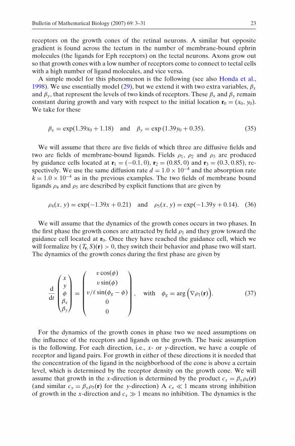
In Fig. 8 we see the fields in a simulation of the model of topographic mapping.The three upper panels show the three diffusive fields ρ1, ρ2 and ρ3.
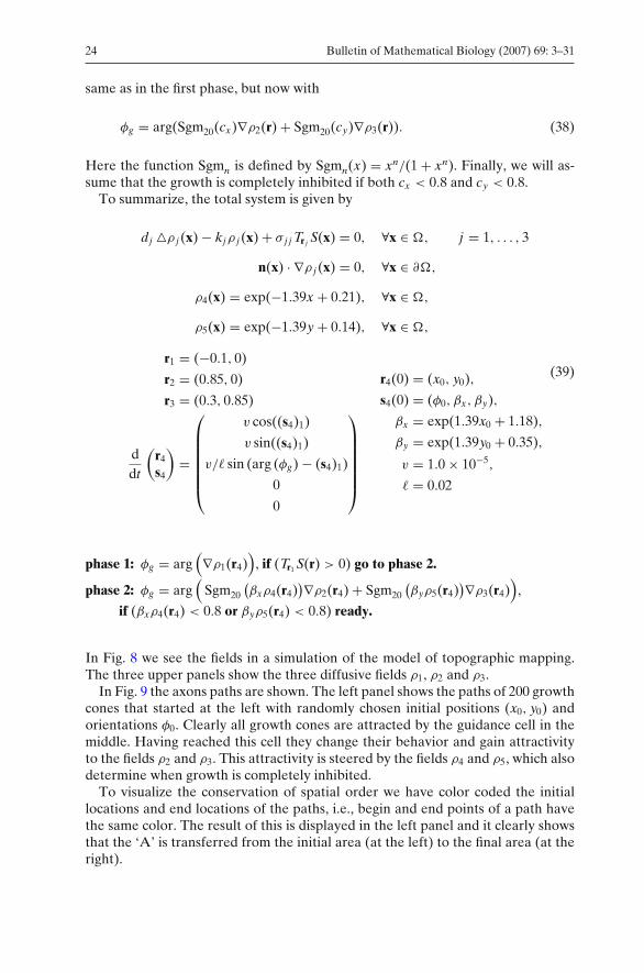
In Fig. 9 the axons paths are shown. The left panel shows the paths of 200 growthcones that started at the left with randomly chosen initial positions (x0, y0) andorientations φ0. Clearly all growth cones are attracted by the guidance cell in themiddle. Having reached this cell they change their behavior and gain attractivityto the fields ρ2 and ρ3. This attractivity is steered by the fields ρ4 and ρ5, which alsodetermine when growth is completely inhibited.
To visualize the conservation of spatial order we have color coded the initiallocations and end locations of the paths, i.e., begin and end points of a path havethe same color. The result of this is displayed in the left panel and it clearly showsthat the ‘A’ is transferred from the initial area (at the left) to the final area (at theright).
Bulletin of Mathematical Biology (2007) 69: 3–31 25
Fig. 8 Fields in the example of topographic mapping. The three fields in the top row are diffusivefields, and the ones in the bottom row are fields of membrane-bound ligands.
The combination of the membrane-bound ligand fields ρ4 and ρ5 with the recep-tor densities βx and βy determines what the topographic mapping will look like.Using a model like this for exploring different possibilities for the concentrationfields can give us more insight into the forms of the fields and mechanisms involvedin topographic map formation.
Fig. 9 Axon paths in the example of topographic mapping. Left: The axons start at the left, andthen grow to the central point, from where they diverge to innervate the target area. Right: Tovisualize that spatial order is conserved when axons innervate their target area, the axons aredivided into two groups (grey and black dots) in such a way that the initial positions of the axonslabeled with the black dots form the pattern ‘A’.
26 Bulletin of Mathematical Biology (2007) 69: 3–31
6. Discussion
In this paper, we have presented a framework for modeling axon guidance. Un-like for the study of electrical activity in neurons and neuronal networks, sucha general framework did not exist. Our framework allows for the relativelystraightforward and fast modeling and simulation of axon guidance and its un-derlying mechanisms. For example, mechanisms that ‘translate’ concentration lev-els of guidance molecules (or gradients thereof), measured at the location of thegrowth cone, into growth speed, growth direction and sensitivity for particular con-centration fields can easily be incorporated. A major challenge in the study of axonguidance is to understand quantitatively how the many molecules and mechanismsinvolved in axon guidance act in concert to generate complex patterns of neuronalconnections. The framework we have developed contributes to this challenge byproviding a general simulation tool in which a wide range of models can be imple-mented and explored.
Our framework has three basic ingredients: the domain, the concentration fieldsand the states. The domain models the physical environment where the neu-rons, axons, and fields live in; the domain can have a complicated geometrywith piecewise smooth boundaries and holes. The fields are defined on the do-main and represent the time varying concentration fields of guidance moleculesthat are subject to diffusion and absorption. The states model the growth conesand targets cells and consist of finite-dimensional vectors for which the dynam-ics are given in the form of ODEs that model the mechanisms involved in axonguidance.
Specific numerical methods have been developed for solving the systems ofequations that typically arise in models of axon guidance. With respect to timeintegration of the full system, a method is needed that can handle the combina-tion of stiff diffusion equations (describing the concentration fields) and non-stiff,nonlinear differential equations (describing the states). For this a second-orderRunge–Kutta IMEX scheme is used. In case of static fields or a quasi-steady-stateapproximation an explicit time integrator will suffice, for which we use the classicalfourth-order Runge–Kutta method.
The spatial discretizations required for solving the elliptic field equations thatarise after discretization in time are based on arbitrary node sets. Voronoi dia-grams are used for the selection of suitable node sets as well as for the discretiza-tion of the equations. To speed up the node selection process, refinement andadaptivity of the discretization are based only upon the location of the highly lo-calized sources.
We have implemented the framework and the numerical algorithms in a setof Matlab programs. In these programs one can simulate a wide range of mod-els by defining appropriate Matlab data-structures and solve them by applyingthe spatial and temporal numerical solvers. At the moment, the code is typ-ical research code without extensive documentation, but we aim to create amore user-friendly version that can be made available to the wider researchcommunity.
Possible extensions of our framework include the incorporation of randomnessin the guidance of the axons and the possibility that boundaries (of impenetrable
Bulletin of Mathematical Biology (2007) 69: 3–31 27
holes, for example) can produce guidance molecules. The latter extension wouldmake it possible to model also tissues, rather than individual cells, that attract orrepel axons.
Appendix
Field set-up time
To examine how the time for setting up the field depends on d and k, we considerthe solution of (3) with a point source at the origin, S(x, t) = δ(x), and an initialfield ρ = 0 at time t = 0. The field will be radially symmetric, and the concentra-tion, which depends only on the radius r and the time t , is
ρ(r, t) =∫ t
0
e−(
ks+ r24ds
)
4πdsds
t→∞−→ 12πd
K0
(r
√kd
), (40)
where the limit of the solution is the steady-state solution, which satisfies (7), andK0 is a modified Bessel function of the Second Kind (Abramowitz and Stegun,1964). To see how fast the field approaches the steady-state field, we will investi-gate
c(r, t) = ρ∞(r) − ρ(r, t)ρ∞(r)
= 1
2K0
(r√
kd
)∫ ∞
2r
√dkt
e− r2
√kd (s+ 1
s )
sds,
which represents how close the field is to its limit value. For example, a valuec(r, t) = 0.01, means that at time t the field is for 99% set up, at location r . Usingan asymptotic expansion for large t for the integral, we find that
c(r, t) ∼ 1
2K0
(r√
kd
) e−kt
kt. (41)
This can be used to get an indication of the time scale of the field dynamics.Such an indicator is important if we want to work with fields of which the sourcesdo not move through the domain. In case of moving sources, one might wonderhow the speed of a source influences the produced field. To this end we examinethe solution of (3) with a point source that moves with constant speed.
Field produced by moving source
Consider Eq. (3) with a point source that moves with constant speed v along the x-axis in positive direction, i.e., S(x, t) = δ(x − vt), with v = (v, 0)T. If we make the‘ansatz’ that the solution ρ(x, t) is the sum of a solution profile ρ that moves with
28 Bulletin of Mathematical Biology (2007) 69: 3–31
constant speed with the source and a ‘residual’ solution η,
ρ(x, t) = ρ(x − vt) + η(x, t),
we can rewrite (11) to
∂
∂tη(x, t) = d �ρ(x − vt) + v · ∇ρ(x − vt) − kρ(x − vt)
+ δ(x − vt) + d �η(x, t) − kη(x, t). (42)
If ρ satisfies the equation
d �ρ(x) + v · ∇ρ(x) − kρ(x) + δ(x) = 0, (43)
we see that Eq. (11) will turn into a equation for η with only diffusion and absorp-tion. Therefore, η will damp out for long times, resulting in ρ(x, t) ≈ ρ(x − vt).The solution of (43) in polar coordinates (r, φ); x = r cos(φ), y = r sin(φ), is givenby
ρ(r, φ) = 12πd
exp
(−
√kd
(v
2√
kd
)r cos(φ)
)
× K0
⎛⎝
√kd
⎛⎝
√(v
2√
kd
)2
+ 1
⎞⎠ r
⎞⎠ . (44)
This solution we will compare to the steady-state solution of (12)
ρs(r) = 12πd
K0
(r
√kd
), (45)
where the subscript s refers to the steady state. So we will consider the quotientfunction q(r, φ) = ρ(r, φ)/ρs(r) and we want to investigate the geometry of theregion where this quotient is close to 1. For example, given a value γ > 1, andslightly bigger than one, we could consider the region {(r, φ) | γ −1 ≤ ρ/ρs ≤ γ }.Using a rescaling of s = r
√k/d and α = v/(2
√dk), we get
q = ρ
ρs= e−αs cos(φ) K0((
√1 + α2)s)
K0(s).
Bulletin of Mathematical Biology (2007) 69: 3–31 29
To analyze q we use the asymptotic expansions of K0 and K1, both modifiedBessel functions of the Second Kind,
K0(x) = ln(2) − ln(x) − γE + O(x2) , K1(x) = 1
x+ O (x) (x ↓ 0), (46)
K0(x) ∼√
π
2xe−x, K1(x) ∼
√π
2xe−x (x → ∞), (47)
where γE is Euler’s constant (Abramowitz and Stegun, 1964).Close to the source, q is close to 1 as follows from lims↓0 q(s, φ) = 1, which can
be seen by using the expansion K0 around 0. To find the behavior around 0, wewill examine the derivative of q with respect to s,
∂sq = q
{K1(s)K0(s)
−√
1 + α2K1(
√1 + α2s)
K0(s)− α cos(φ)
}.
This is equal to q times some factor that is increasing with s and has limit values−∞ at s = 0 and 1 − √
1 + α2 − α cos(φ) at s = ∞. For φ = 0 this limit is negative,while for φ = π this limit is positive. Therefore, there is an interval [−φt , φt ] withφt ∈ [0, π] of possible choices of φ for which q decreases with s while keeping φ
constant.For φ outside this interval, i.e., φ ∈ (−π,−φt ) ∪ (φt , π], there is an sφ > 0, with
∂sq(sφ, φ) = 0, such that q as a function of s decreases for s ∈ (0, sφ) and increasesfor s ∈ (sφ,∞). The function φ → sφ itself is decreasing on (φt , π] with limφ↓φt sφ =∞. To find φt ∈ [0, π ], we solve
1 −√
1 + α2 − α cos(φt ) = 0, =⇒ cos(φt ) = 1 − √1 + α2
α< 0,
where the last inequality follows from the fact that α > 0. Therefore, φt ∈ ( 12π, π),
which is increasing with α and has limits φt = 12π with α ↓ 0 and φt = π for α → ∞.
We can now conclude that close to the origin there is some region where wehave q ≤ 1. To find an estimate for the size of this region we will use the asymptoticexpansion of q for small s,
q = 1 +12 ln(1 + α2)
ln(s) − ln(2) + γE+ O (s) .
Neglecting the higher-order terms and setting this equal to γ gives
s = 2e−γE (1 + α2)1
2(γ−1) =⇒ r = 2e−γE
√dk
(1 + v2
4dk
) 12(γ−1)
. (48)
If we choose γ = 0.99, we get an indication for the region around the sourcewhere the difference between the moving profile and the quasi-steady-state
30 Bulletin of Mathematical Biology (2007) 69: 3–31
solution is smaller than 1%, given the values of the diffusion rate d, absorptionrate k and moving speed v.
References
Abramowitz, M., Stegun, I.A. (Eds.), 1964. Handbook of Mathematical Functions. Dover Publi-cations, New York.
Atkinson, K., Han, W., 2001. Theoretical Numerical Analysis. Number 39 in Texts in AppliedMathematics. Springer-Verlag, New York.
de Berg, M., van Kreveld, M., Overmars, M., Schwarzkopf, O., 2000. Computational Geometry,2nd edition. Springer-Verlag.
Dickson, B.J., 2002. Molecular mechanisms of axon guidance. Science 298, 1959–1964.Dodd, J., Jessell, T.M., 1988. Axon guidance and the patterning of neuronal projections in verte-
brates. Science 242, 692–699.Du, Q., Faber, V., Gunzburger, M., 1999. Centroidal Voronoi tessellations: Applications and al-
gorithms. SIAM Rev. 41(4), 637–676.2002Fortune, S., 1987. A sweepline algorithm for Voronoi diagrams. Algorithmica 2, 153–174.Gaze, R.M., 1958. The representation of the retina on the optic lobe of the frog. Quart. J. Exp.
Physiol. 43, 209–224.Goodhill, G.J., 1997. Diffusion in axon guidance. Eur. J. Neurosci. 9, 1414–1421.Goodhill, G.J., 1998. A mathematical model of axon guidance by diffusible factors. In: Jordan,
M.I., Kearns, M.J., Solla, S.A. (Eds.), Advances in Neural Information Processing Systems,vol. 10. MIT Press, pp. 159–165.
Hentschel, H.G.E., van Ooyen, A., 1999. Models of axon guidance and bundling during develop-ment. Proc. R. Soc. Lond. B. 266, 2231–2238.
Hines, M.L., Carnevale, N.T., 1997. The neuron simulation environment. Neural Comput. 9, 1179–1209.
Honda, H., 1998. Topographic mapping in the retinotectal projection by means of complementaryligand and receptor gradients: A computer simulation study. J. Theor. Biol. 192, 235–246.
Huber, A.B., Kolodkin, A.L., Ginty, D.D., Cloutier, J.-F., 2003. Signaling at the growth cone:Ligand–receptor complexes and the control of axon growth and guidance. Annu. Rev. Neu-rosci. 26, 509–563.
Hundsdorfer, W., Verwer, J.G., 2003. Numerical Solution of Time-Dependent Advection–Diffusion–Reaction Equations. Springer.
Krottje, J.K., 2003a. On the dynamics of a mixed parabolic-gradient system. Commun. Pure Appl.Anal. 2(4), 521–537.
Krottje, J.K., 2003b. A variational meshfree method for solving time-discrete diffusion equations.Technical Report MAS-E0319, Centrum voor Wiskunde en Informatica, P.O. Box 94079,1090 GB Amsterdam, The Netherlands, December 2003.
Lastdrager, B., 2002. Numerical solution of mixed gradient-diffusion equations modeling axongrowth. Technical Report MAS-R0203, Centrum voor Wiskunde en Informatica, P.O. Box94079, 1090 GB Amsterdam, The Netherlands, January 2002.
Ming, G.-L., Henley, J., Tessier-Lavigne, M., Song, H.J., Poo, M.-M., 2001. Electrical activity mod-ulates growth cone guidance by diffusible factors. Neuron 29, 441–452.
Ming, G.-L., Wong, S.T., Henley, J., Yuan, X.-B., Song, H.-J., Spitzer, N.C., Poo, M.-M., 2002.Adaptation in the chemotactic guidance of nerve growth cones. Nature 417, 411–418.
O’Leary, D.D.M., Wilkinson, D.G., 1999. Eph receptors and ephrins in neural development. Curr.Opin. Neurobiol. 9, 55–73.
Rehder, V., Kater, S.B., 1996. Filopodia on neuronal growth cones: Multi-functional structureswith sensory and motor capabilities. Sem. Neurosci. 8, 81–88.
Shewan, D., Dwivedy, A., Anderson, R., Holt, C.E., 2002. Age-related changes underlie switchin netrin-1 responsiveness as growth cones advance along visual pathway. Nat. Neurosci. 5,955–962.
Shirasaki, R., Katsumata, R., Murakami, F., 1998. Change in chemoattractant responsiveness ofdeveloping axons at an ntermediate target. Science 279, 105–107.
Song, H., Ming, G., He, Z., Lehmann, M., Tessier-Lavigne, M., Poo, M.-M., 1998. Conversion ofneuronal growth cone responses from repulsion to attraction by cyclic nucleotides. Science281, 1515–1518.

Bulletin of Mathematical Biology (2007) 69: 3–31 31
Song, H.-J., Poo, M.-M., 1999. Signal transduction underlying growth cone guidance by diffusiblefactors. Curr. Opin. Neurobiol. 9, 355–363.
Tessier-Lavigne, M., Goodman, C.S., 1996. The molecular biology of axon guidance. Science 274,1123–1133.
van Ooyen, A. (Ed.), 2003. Modeling Neural Development. MIT Press.Verwer, J.G., Sommeijer, B.P., 2001. A numerical study of mixed parabolic-gradient systems. J.
Comp. Appl. Math. 132, 191–210.Wilkinson, D.G., 2001. Multiple roles of eph receptors and ephrins in neural development. Nat.
Neurosci. Rev. 2, 155–164.Yamamoto, N., Tamada, A., Murakami, F., 2003. Wiring up the brain by a range of guidance cues.
Progress Neurobiol. 68, 393–407.Young, S., Poo, N.M., 1983. Spontaneous release of transmitter from growth cones of embryonic
neurons. Nature 305, 634–637.Zheng, J.Q., Felder, M., Connor, J.A., Poo, M.M., 1994. Turning of nerve growth cones induced
by neurotransmitters. Nature 368, 140–144.Zou, Y., Stoeckli, E., Chen, H., Tessier-Lavigne, M., 2000. Squeezing axons out of the gray matter:
A role for slit and semaphorin proteins from midline and ventral spinal cord. Cell 102, 363–375.