A low-cost custom knee brace - uO Research

A LOW-COST CUSTOM KNEE BRACE VIA

SMARTPHONE PHOTOGRAMMETRY

Olivier Miguel

A thesis submitted to the Faculty of Graduate and Postdoctoral Studies in partial fulfillment of the requirements for the degree of

MASTER OF APPLIED SCIENCE

in Biomedical Engineering

Ottawa-Carleton Institute for Biomedical Engineering University of Ottawa

Ottawa, Canada

January 2019

© Olivier Miguel, Ottawa, Canada, 2019

ii

Table of Contents 1 ABSTRACT ........................................................................................................................................... VIII 2 INTRODUCTION...................................................................................................................................... 1

2.1 BACKGROUND/MOTIVATION............................................................................................................... 1 2.2 RESEARCH OBJECTIVE AND SIGNIFICANCE ......................................................................................... 4 2.3 DESIGN REQUIREMENTS...................................................................................................................... 5

2.3.1 Functional requirements ............................................................................................................... 5 2.3.2 Non-functional requirements ......................................................................................................... 5

2.4 CONTRIBUTIONS .................................................................................................................................. 6 3 LITERATURE REVIEW ......................................................................................................................... 8

3.1 KNEE BIOMECHANICS ......................................................................................................................... 8 3.2 TYPES OF KNEE BRACES/KNEE BRACE DESIGNS .................................................................................. 8

3.2.1 Prophylactic vs Functional Knee braces ....................................................................................... 9 3.2.2 Types of Joint Designs ................................................................................................................. 10

3.3 CUSTOM VS PREFABRICATED KNEE BRACES .................................................................................... 11 3.4 ORTHOTICS ADDITIVE MANUFACTURING EVOLUTION ..................................................................... 12

3.4.1 Knee Orthotics ............................................................................................................................. 13 3.4.2 Foot Orthotics ............................................................................................................................. 13 3.4.3 Ankle-Foot Orthotics ................................................................................................................... 18 3.4.4 Lower-limb prosthetic sockets ..................................................................................................... 21 3.4.5 Other 3D Printed Assistive Devices ............................................................................................ 23

3.5 ADDITIVE MANUFACTURING ............................................................................................................ 23 3.5.1 Types of 3D Printing ................................................................................................................... 23 3.5.2 FDM Model Parameters .............................................................................................................. 25

3.6 TYPES OF 3D SCANNING ................................................................................................................... 27 3.6.1 High-cost Scanners ...................................................................................................................... 28 3.6.2 Low-cost Scanners ....................................................................................................................... 28 3.6.3 Photogrammetry/Structure from motion ..................................................................................... 29

4 WORKFLOW DEVELOPMENT .......................................................................................................... 32 4.1 OVERVIEW ........................................................................................................................................ 39 4.2 SMARTPHONE PHOTOGRAMMETRY METHOD .................................................................................... 33

4.2.1 Leg scan procedure (Data collection) ......................................................................................... 33 4.2.2 Photogrammetry Software ........................................................................................................... 43 4.2.3 Mesh Processing .......................................................................................................................... 36

4.3 COMPUTER ASSISTED DESIGN METHOD ........................................................................................... 39 4.3.1 Development of Hinge Design ..................................................................................................... 40 4.3.2 Digital Alignment & Brace Cuff Design ..................................................................................... 43

4.4 3D PRINTING METHOD ...................................................................................................................... 53 4.4.1 Orientation .................................................................................................................................. 53 4.4.2 Printing Parameters .................................................................................................................... 54 4.4.3 Material ....................................................................................................................................... 55 4.4.4 Assembly ...................................................................................................................................... 55

4.5 PROTOTYPING ................................................................................................................................... 56 4.5.1 Prototype 1 .................................................................................................................................. 56 4.5.2 Prototype 2 .................................................................................................................................. 58

5 VALIDATION STUDY – SMARTPHONE PHOTOGRAMMETRY ............................................... 61 5.1 EXPERIMENTAL DESIGN AND DATA COLLECTION ............................................................................ 61 5.2 DATA PROCESSING ............................................................................................................................ 62

iii

5.3 STATISTICAL ANALYSIS .................................................................................................................... 64 5.4 RESULTS............................................................................................................................................ 64

5.4.1 Validity ........................................................................................................................................ 65 5.4.2 Reliability .................................................................................................................................... 69

5.5 DISCUSSION....................................................................................................................................... 71 6 CONCLUSION AND FUTURE WORK ............................................................................................... 74

6.1 SUMMARY ......................................................................................................................................... 74 6.2 RECOMMENDATIONS/FUTURE WORK................................................................................................ 74

7 APPENDIX ............................................................................................................................................... 77 7.1 PYTHON SCRIPTS ............................................................................................................................... 77

7.1.1 meshlabserverPyAuto.py ............................................................................................................. 77 7.1.2 importKJCdata.py ....................................................................................................................... 95

7.2 SMARTPHONE CAMERA SCANNING PROCEDURE STEP-BY-STEP ......................................................... 97 7.3 MESH PROCESSING STEP-BY-STEP ..................................................................................................... 98 7.4 FUSION 360 STEP-BY-STEP ................................................................................................................ 99

8 REFERENCES ....................................................................................................................................... 102

iv

List of Abbreviations 3D: Three-Dimensional

3DP: 3-Dimensional Printing

ABS: Acrylonitrile Butadiene Styrene

AFO: Ankle-Foot Orthotic

AM: Additive Manufacturing

Ant-Post: Anterior-Posterior

BBox: Bounding Box

CAD: Computer Assisted Design or Canadian Dollar

CC: Calf Cuff

DoF: Degree of Freedom

FDM: Fused Deposition Modelling

FO: Foot Orthotic

HD: Hausdorff Distance

ICR: Instantaneous Center of Rotation

KJC: Knee Joint Center

Med-Lat: Medial-Lateral

MP: Megapixels

O&P: Orthotics & Prosthetics

PA: Polyamide

PEEK: Polyether Ether Ketone

PEI: Polyetherimide

PETG: Polyethylene Terephthalate

PLA: Polylactic Acid

Prox-Dist: Proximal-Distal

SLS: Selective Laser Sintering

STL: Stereolithography

TC: Thigh Cuff

TPU: Thermoplastic Polyurethane

v

List of Figures Figure 1 - Photogrammetry DSLR tower frame .................................................................................................. 30 Figure 2 – Workflow. A smartphone was used to record multiple views of the leg. The recorded frames were

then uploaded to the Autodesk Recap cloud-based software. The software outputs a textured mesh using

photogrammetry algorithms. The output mesh was cropped, smoothed and then used to design a 3D

printable custom knee brace....................................................................................................................... 32 Figure 3 – a) Lateral, b) anterior, c) medial, and d) posterior views of the left lower extremity captured from the

smartphone video. ...................................................................................................................................... 35 Figure 4 – Left, typical photogrammetry camera tower rig. Right, smartphone camera path chosen to emulate the

camera tower rig as best as possible while ensuring optimal recordings. ................................................. 35 Figure 5 - Five plane cut sequence with end result. The first four are plane cuts around the A4 paper perimeter

and the fifth plane cut is perpendicular to the thigh axis. The end result only contains the lower extremity

of interest. .................................................................................................................................................. 37 Figure 6 - Measuring, scaling and verifying the scale of the A4 paper. The first measurement, taken from the

longest side of the A4 paper is 0.559 cm. It should measure 27.9 cm which is 5000% bigger. After applying

a scaling factor of 5000% the long side of the A4 paper measured 27.94 cm. .......................................... 37 Figure 7 – Mesh1 plane cut removing A4 paper and foot to create Mesh2 ........................................................ 38 Figure 8 - a) Mesh2 before smoothing b) Mesh3 after applying a laplacian smoothing modifier ...................... 39 Figure 9 - a) Exploded view of the bicentric hinge design. b) Full extension side view without the Cap. ......... 42 Figure 10 - Spur gear script parameters............................................................................................................... 43 Figure 11 - Mesh1 position in Fusion 360. Left shows the origin (0,0,0) with the 3D axes (blue, red, and green),

the three planes (top, front, side), the A4 paper sketch and Mesh1. Middle shows the top plane cutting

through Mesh1 at the height between the lateral and medial malleolus. Right shows that Mesh1’s scale

matches the A4 paper dimension sketch (units are in mm). ...................................................................... 44 Figure 12 – a) Creation of T1 by converting mesh3 from quad mesh to T-spline surface. b) Inward thickening

of T1 by 5mm with soft edges. c) Finish form button. d) Resulting body B1. .......................................... 45 Figure 13 – a) Sketch determining the knee joint center. b) Knee brace side sketch template. c) Result of the

extrude include operation. All units are in mm.......................................................................................... 46 Figure 14 - a) Left hinge alignment with sketch1 line segments b) Left hinge distance from mesh1 c) Right hinge

distance from mesh1 .................................................................................................................................. 46 Figure 15 – a) Thigh cuff (top) and calf cuff (bottom) before fillets. b) After fillets ......................................... 47 Figure 16 - Eight faces used to make the four lofts are outlined in magenta and the 3D sketch guide curves are

in blue......................................................................................................................................................... 48 Figure 17 – Brace cuffs combined with the 4 bodies created by the lofts gives the cuffs with complete sidebars

.................................................................................................................................................................... 48 Figure 18 - Side sketch of slot holes. All dimensions are in mm. ....................................................................... 49 Figure 19 - Rectus femoris EMG hole ................................................................................................................ 50

vi

Figure 20 - Gastrocnemius medialis and lateralis EMG holes ............................................................................ 51 Figure 21 - Brace cuffs ready for additive manufacturing .................................................................................. 52 Figure 22 - Top, thigh cuff orientation. Bottom, calf cuff orientation ................................................................ 53 Figure 23 - Right hinge print orientation ............................................................................................................. 54 Figure 24 – Cura hinge print job parameter settings ........................................................................................... 55 Figure 25 - Manual bending method. Thumbs are placed in the center of the hinge and the hands are pulling

down on the ends of the geared segments .................................................................................................. 58 Figure 26 - Computer assisted-design of Prototype 2. The EMG sensor case is merged with the brace cuffs. .. 59 Figure 27 - Bicep brachii muscle EMG signals collected with the electronic prototype. ................................... 60 Figure 28 – Frame extracted from the video recording. Plastic coins on the leg were used to aid in mesh

reconstruction and processing .................................................................................................................... 62 Figure 29 – Cropped leg showing the proximal (thigh) and distal (ankle) clusters used for cropping. .............. 63 Figure 30 - Bland-Altman plot of the volume measurements. Top is the absolute difference between the

smartphone photogrammetry and the iSense sensor. Bottom is the error of the smartphone volume

measurements expressed as a percentage of the volume average. A negative value represents that the

smartphone underestimates the volume with respect to the iSense sensor. The solid lines represent the

mean of the differences and the mean of the errors. The dashed lines represent the upper and lower 95%

limits of agreement. ................................................................................................................................... 66 Figure 31 – Bland-Altman plots for the cross-sectional area (CSA) measurements of the thigh. Top is the absolute

difference between the smartphone photogrammetry and the iSense sensor. Bottom is the error of the

smartphone measurements expressed as a percentage of the average. A negative value represents that the

smartphone underestimates the CSA with respect to the iSense sensor. The solid lines represent the mean

of the differences and the mean of the errors. The dashed lines represent the upper and lower 95% limits

of agreement............................................................................................................................................... 67 Figure 32 - Bland-Altman plots for the cross-sectional area (CSA) measurements of the shank. Top is the absolute

difference between the smartphone photogrammetry and the iSense sensor. Bottom is the error of the

smartphone measurements expressed as a percentage of the average. A negative value represents that the

smartphone underestimates the CSA with respect to the iSense sensor. The solid lines represent the mean

of the differences and the mean of the errors. The dashed lines represent the upper and lower 95% limits

of agreement............................................................................................................................................... 68 Figure 33 - Hausdorff distance color map of the two best scans obtained with the smartphone photogrammetry

method. The left side shows the Hausdorff distance distribution in cm. Red means 0 distance and blue

means the distance is > 5mm. .................................................................................................................... 73

vii

List of Tables Table 1 - Limb overall measurements. HD = Hausdorff Distance ...................................................................... 65 Table 2 - Validity Results. BBox = Bounding Box measurements, Ant-Post = anterior-posterior axis, Med-Lat =

medial-lateral axis, Prox-Dist = proximal-distal axis, KJC = knee joint center coordinates. .................... 69 Table 3 - Intra-rater reliability results. BBox = Bounding Box measurements, Ant-Post = anterior-posterior axis,

Med-Lat = medial-lateral axis, Prox-Dist = proximal-distal axis, KJC = knee joint center coordinates. . 70 Table 4 - Inter-rater reliability results. BBox = Bounding Box measurements, Ant-Post = anterior-posterior axis,

Med-Lat = medial-lateral axis, Prox-Dist = proximal-distal axis, KJC = knee joint center coordinates. . 70

viii

Abstract

This thesis provided the foundational work for a low-cost three-dimensional (3D) printed

custom knee brace. Specifically, the objective was to research, develop and implement a novel

workflow aimed to be easy to use and available to anyone who has access to a smartphone

camera and 3D printing services. The developed workflow was used to manufacture two

prototypes which proved valuable in the design iterations. As a result, an improved hinge was

designed which has increased mechanical strength. Additionally, a smartphone

photogrammetry validation study was included which provided preliminary results on the

accuracy and precision. This novel measurement method has the potential to require little

training and could be disseminated through video instructions posted online. The intention is

to enable the patient to collect their own “3D scan” with the help of a friend or family member,

effectively removing the need to book an appointment simply for collecting custom

measurements. Lastly, it would allow the clinician to focus all their time on clinically relevant

design tasks such as checking alignment, fit and comfort, which could all potentially be

improved by adopting such digital methods. The ultimate vision for this work is to enable

manufacturing of better custom knee braces at a reduce cost which are easily accessible for

low-income populations.

1

1 Introduction

1.1 Background/Motivation

Sports-related knee injuries are increasing and have reached an epidemic level in

children [1], [2]. The knee is one of the more commonly injured joints of the body. In fact it

is reported to be the most commonly injured joint for youth participating in sports [3] and is

often more severe than other joint injuries of the body [4]. They typically require surgery or

extensive rehabilitation before the knee joint can function at pre-injury levels. Interestingly,

many are non-contact in nature, and occur during activities such as rapid decelerations and

side-cuts [5]. Unfortunately, regardless of whether the patient seeks non-operative or

operative rehabilitations, these injuries are associated with long-term health consequences

such as the increased likelihood (up to 71%) of developing knee osteoarthritis (OA) [6]–[9]

and a 12-24% chance of re-injury [10]–[13]. Together these lasting consequences result in

low return to pre-injury activity levels, and ultimately reduce quality of life [6], [14].

In Canada the current protocol for pediatric knee injuries is physiotherapy and

prescribing a functional knee brace. The decision of the latter is left to the physician’s

discretion [15]. A functional knee brace is prescribed to facilitate rehabilitation of the joint.

Despite their use, the benefits associated with knee braces are still unclear [16]–[21]. Knee

braces have been linked to increased hamstring and decreased quadriceps muscle activity [16],

thigh muscle atrophy [17], decreased hamstring activity [22], and premature muscle fatigue

[19]. A hypothesis is that the muscle impairments are a result of the brace straps creating

external compression on the muscles which can decrease blood flow and result in poor

oxygenation [19].

On the positive side, knee braces have been shown to 1) prevent excessive loading [20],

2) increase joint proprioception [20] and 3) improve confidence of the wearer [21]. The first

is currently addressed with joint designs having a hyper-extension lock (see Types of Joint

Designs). Increased proprioception or kinesthesia is helpful in preventing bad joint positions

and injury [23], [24]. This kinesthesia could be enabled via increased activity of the

2

proprioceptive sensors around the knee (e.g. mechanoreceptors on the skin) caused by forces

due to the weight, inertia and restricted motion (flexion/extension) of the brace.

Among this controversy over the effectiveness of bracing, their cost creates even more

unease in their use. A custom knee brace cost approximately 1500 CAD [25]. This cost is

prohibitive for many, unless it is covered partially or completely by third party insurance

policies. In fact, a Canadian survey discovered that 26% of patients who received a functional

knee brace prescription did not end up purchasing one [26]. The reported effects of knee

braces are therefore not convincing enough for the high cost especially in pediatrics cases

where the patient may require multiple braces as he/she grows.

This high cost of custom knee braces primarily comes from the custom manufacturing

process. The current manufacturing models of the large knee brace companies is to mass

produce in a central location [27]. This works well for prefabricated braces but is not as

effective for mass customization. A decentralized manufacturing model is more flexible and

effective for mass production of customized products [28], [29].

Additive manufacturing (AM) commonly known as three-dimensional printing (3DP)

has enabled many businesses to adopt a decentralized manufacturing model for mass

customization. The first invention was patented in 1984 [30] however it is the recent low-cost

desktop 3D printers that brought AM into mainstream knowledge. Desktop 3D printers range

from 200CAD – 8000CAD making this approach more accessible than ever for individuals

and small businesses [31], [32].

A key advantage of AM is that it opens design possibilities. In other words, it enables

design freedom. Design freedom means that any shape can now be manufactured without

additional cost attributed to manufacturing complexity. This is the reason why this technology

has gained attention in medicine. The promise of using 3DP in medicine is that it will enable

a new level of patient-specific healthcare and as a result, it has gained attention in the

prosthetics and orthotics field. What is less known however, is that 3DP of orthotic devices

has been a focus of medical and rehabilitation research for more than 25 years [33]. People

have created prosthetic hands, prosthetic sockets, foot orthotics, ankle-foot-orthotics and more

(see Orthotics Additive Manufacturing). The projects involved the development of new

methods that can manufacture medical devices at a reduce cost. Additionally, by shifting

manufacturing from a manual to a digital process (i.e.: 3D printers), novel devices have the

3

potential for an improved fit and comfort. A leader in this space is Nia technologies which is

working with three clinical partners in different developing countries to increase clinician

productivity by facilitating the adoption of these new digital methods for manufacturing

orthotics and prosthetics (O&P) [34]. Another, “Enabling The Future” successfully

decentralized manufacturing which enabled the provision of medical devices to individuals

who previously did not have access [35]. The common vision: to make medical devices more

accessible and affordable. With the easy deployment of low-cost desktop 3D printers, these

technologies became vastly more accessible.

AM was not the sole reason why the accessibility of these devices increased. A change

in the customization process more specifically the measurement taking method was also

necessary. The traditional measurement method for custom knee braces employs a measuring

tape which is cheap, simple, and accurate; however, the inter- and intra-rater reliability is poor

[36]. Similarly, Enabling The Future’s measurement method is a series of pictures of the limb

of interest with a reference scale [37]. These pictures are used to remotely measure anatomical

dimensions and scale the prosthetic parametric designs, however; it is not optimal since it

cannot be used for all O&P. For example, prosthetic sockets (and ankle-foot-orthotics) require

the full limb geometry to create a high quality and properly functioning device. Traditionally

this is achieved with the plaster and molding technique. This is a tedious and repetitive manual

labour process and is not the most time effective. Fortunately, the full limb geometry can be

acquired digitally with 3D scanning.

Some clinics now use high-end 3D scanners which provide an accurate and reliable way

to digitize the shape of the leg [38], [39]. This approach enables higher customization and

more design possibilities however; their high cost makes them inaccessible to many

practitioners. More recently, there has been the development of low-cost 3D scanners like the

iSense sensor (3D Systems, Rock Hill, South Carolina, United States) which uses a depth

sensor mounted on an iPad (Apple, Cupertino, California, United States). These devices are

more affordable and accessible and have recently been demonstrated to provide good accuracy

and reliability (ICC = 0.99) [38]. However, all of these measurement methodologies are still

performed by the practitioner who needs additional training to use them. The practitioner’s

time is too valuable. Ideally, the practitioner does not need to perform any manufacturing tasks

4

and instead focuses all their efforts on clinically relevant tasks such as checking alignment, fit

and comfort.

There exists a method which has the potential to enable 3D scanning using only a camera

and internet connection: cloud-based photogrammetry. Photogrammetry has been around

since the mid 19th century [40] but with the recent technological advancements in computer

vision, pattern recognition, processing power, and world-wide internet access, every camera

now has the potential to be used as a 3D scanner. Additionally, video instructions could be

followed requiring little training allowing anyone with a camera (i.e.: the patient) to digitize

the shape of the leg. This could enable the patient to collect their own “3D scan” with the help

of a friend or family member and send it wirelessly effectively removing the need to book an

appointment just for collecting anatomical measurements. Ultimately, the brace could be self-

fitting and fit verification could also be done via video training. Consequently, we believe that

smartphone photogrammetry combined with 3DP could be a viable low-cost approach for

manufacturing O&P specifically custom knee braces.

1.2 Purpose, Research Objective and Significance

The purpose of this thesis is to provide the foundational work for a low-cost 3D printed

custom knee brace. Specifically, the research, development and implementation of a novel

workflow aimed to be easy to use and available to anyone who has access to a smartphone

camera and 3D printing services.

The objectives of this thesis are to 1) establish a workflow to manufacture a low-cost

3D printed custom knee brace targeted to pediatric populations and 2) begin the validation

process of this workflow. To the best of our knowledge, there hasn’t been any study

investigating smartphone photogrammetry for digitizing the knee, in particular digitizing with

the goal of providing a useful map for knee brace customization. Therefore, to begin the

validation, the accuracy and precision (validity and reliability) of the smartphone

photogrammetry method will be assessed using an accurate and reliable 3D scanner (iSense

sensor) as the criterion.

This workflow is a bootstrap approach to manufacture and prototype custom knee

braces. It can enable clinicians, engineers, researchers and biomechanists to manufacture

5

prototypes at a low-cost, as well as improve the future of custom knee brace manufacturing.

A 3D printed custom knee brace can have significant impact for the pediatric population since

multiple braces need to be manufactured as the patient grows (cost savings are multiplied).

1.3 Design Requirements

A possible solution to the problem detailed above was discussed with a focus group.

The focus group included Dr. Daniel Benoit, who is an expert in clinical biomechanics and

Dr. Sasha Carsen an orthopaedic surgeon from the Children’s Hospital of Eastern Ontario.

The following functional and non-functional requirements were established for the envisioned

solution. The focus of this thesis was on the functional requirements. The non-functional

requirements were not fully met by the current state of the development however they have

guided the technology choices for the steps in the workflow.

1.3.1 Functional requirements

1. Generate 3D scan of the full leg

2. Generate a digital custom knee brace which

a. Has a knee extension limit to prevent hyper-extension

b. Has bilateral uprights to meet multiple knee brace categories

c. Has a polycentric hinge to follow proper knee joint biomechanics (see Types

of Joint Designs)

d. Has a large skin contact surface to

i. Cover EMG sensor placements for instrumentation

ii. Provide better comfort/fit by distributing the forces over a large surface

3. Determine preliminary 3D printing parameters

1.3.2 Non-functional requirements

1. Usability

6

a. End user may have low expertise level and can follow an online

instructional video to scan the knee and fit the brace. The brace is self-

fitted.

2. Accessibility

a. Scanning of the knee is done by anybody with a smartphone camera

b. Use free and/or open-source software

c. Low-cost production targeting low-income families and countries.

i. Material cost is low by using 3D printed plastics.

ii. The labour cost is low by automating the computer-aided design

(CAD) process

d. Initial target market is for pediatrics.

3. Scalability

a. Global scale through a decentralized manufacturing business model

4. Reliability

a. Output of the workflow is consistent for the same individual. Scanning

method and the orthopaedic alignment are arguably the most important for

assessing the reliability.

i. Multiple 3D scans for the same leg should be consistent with a

maximum Hausdorff Distance ≤ 2cm. Based on sizing charts for

currently available custom knee brace products the smallest

measurement range is 2cm [41]–[44]. Padding can be added to

reduce gaps.

ii. The feature extraction of the anatomical alignment should be

consistent with a maximum error of 5mm to ensure proper hinge

placement [45].

b. The 3D printed brace can be used in high impact scenarios such as during

sports

1.4 Contributions

This thesis focused on establishing the foundation of a novel approach for a low-cost 3D

printed custom knee brace workflow. The functional requirements were identified and a

7

design which fulfills these was researched, designed and implemented. The contributions are

the research, development, and implementation of

1) a smartphone photogrammetry method for digitizing the knee (see Smartphone

Photogrammetry Method)

2) a computer assisted design (CAD) method for a functional knee brace (see Computer

Assisted Design )

3) additive manufacturing preliminary optimal parameters (see 3D Printing Method)

Additionally, two functional prototypes were built and tested which led to the design and

implementation of

4) an improved 3D printed polycentric hinge (see Prototype 1)

a. Designed by Hilal Edrogen and Olivier Miguel.

b. Manufactured by Olivier Miguel.

5) an EMG instrumented knee brace prototype (see Prototype 2)

a. The electronic prototype was created by Ahmed Jaber an undergraduate

student from University of Ottawa

b. The instrumented brace prototype was designed by Olivier Miguel

Finally, to begin validating the workflow a systematic/quantitative contribution is included:

6) validation study of the smartphone photogrammetry method for digitizing the knee

(see Validation Study – Smartphone Photogrammetry)

8

2 Literature Review

2.1 Knee Biomechanics

The knee is a six degree of freedom (DoF) joint with its primary motion being

flexion/extension in the sagittal plane. It is often compared to a hinge with a constantly

changing centre of rotation [46]. The instantaneous centre of rotation follows a spiral-like path

[46], which is called polycentric rotation and occurs due to an anatomical phenomenon called

femoral rollback. Femoral rollback is the rolling and sliding of the femoral condyles on the

tibia plateau (Figure 25.1 in [47]). When the knee begins flexion from full extension, rolling

of the femoral condyles begins with minimal sliding. As the flexion angle deepens the sliding

motion increases and eventually becomes predominant [47].

The knee also undergoes axial rotation termed the screw home mechanism [48] where

in the last few degrees of extension, the tibia externally rotates relative to the femur. This

motion occurs due to the different shapes of the tibial plateau surfaces. The medial surface is

slightly concave anteriorly while the lateral surface is convex also anteriorly. The concavity

on the medial surface stops the rolling medial femoral condyle while the convex slope of the

lateral surface allows the lateral femoral condyle to continue forward. The resulting motion is

a medial rotation of the femoral shaft [49].

There are four ligaments which provide passive mechanical constraints to the six DoF

knee joint: the anterior cruciate ligament (ACL), the posterior cruciate ligament (PCL), the

medial collateral ligament (MCL) and the lateral collateral ligament (LCL). Accordingly, the

ACL and PCL primarily restrain anterior and posterior translation of the tibia relative to the

femur. The MCL and LCL primarily prevent excessive valgus and varus motion respectively

[50]. As a result of these mechanical constraints, the path of the knee instantaneous centre of

rotation (ICR) has been compared to a spiral in the sagittal plane [46].

2.2 Types of knee braces/Knee brace designs

Knee braces are designed to transfer loads while allowing normal knee motion. Longer

knee braces can apply more leverage to the limb [51] and where the leverage is applied

depends on the objective of the knee brace. A rigid brace is designed to act like a 3-point

bending protection/reinforcement for the knee. The energy from a lateral impact is absorbed

9

by the brace into material deformation. As the elastic deformation springs back, it applies

distributed forces onto the limb higher on the thigh and lower on the shank. Material

deformation is largest at the load site and attachments points are the most mechanically

susceptible for deformation (i.e.: hinges are the most susceptible to break) [47].

Currently there is an abundance of knee brace categories on the market; however, three

main categories emerge from the literature: 1) Functional and/or Prophylactic, 2)

Osteoarthritis off-loader and 3) Patellofemoral [47]. Most categories are available in soft or

rigid material and custom or prefabricated designs.

The functional/prophylactic knee brace was the chosen design to demonstrate the

process of a 3D printed custom knee brace. It was chosen since: 1) it is currently prescribed

for pediatric sport injuries, 2) a 3D printed custom knee brace can have significant impact for

the pediatric population since multiple braces need to be manufactured as the patient grows

(cost savings are multiplied) and 3) the available desktop 3D printers for the project have build

platforms which were too small for large thighs (e.g. osteoarthritis patients).

2.2.1 Prophylactic vs Functional Knee braces

Prophylactic knee braces are used to protect the knee from injury. Athletes playing in

sports with high risk of the knee injury (i.e. football, soccer) wear them as a preventative

measure [52]. The designs use polycentric hinges in a unilateral/single-hinge arrangement or

bilateral uprights arrangement [47]. These apply leverage on the thigh and shank keeping the

knee from excessive valgus and the MCL from overstraining [47]. If the brace is impacted on

the hinge or close to the knee, the brace transfers the load away from the knee joint to a larger,

more distal and proximal region on the shank and thigh (Figure 25.3 in [47]).

Functional knee braces are prescribed to stabilize a patient’s knee after suffering a

knee injury such as an ACL rupture. These primarily apply leverage to prevent excessive

forward translation motion of the tibia relative to the femur [53]. Their effectiveness is still

debated; however, past studies have shown that it can provide increased mechanical stiffness

to the knee for low physiological loads [15], [54]–[59]. These braces include polycentric

hinges and bilateral uprights. All functional knee brace designs can be prescribed as a

prophylactic knee brace; however, not all prophylactic knee brace designs can be prescribed

10

as a functional knee brace [47]. Specifically, if a knee brace has bilateral uprights it can be

classified as both types [47]. The commonality between the two is that they are used to assist

the knee joint’s ligaments: the MCL for prophylactic braces and the ACL for functional braces

[47].

2.2.2 Types of Joint Designs

The hinge design is a critical component which determines if the knee brace will

function properly. Excessive motion between the brace and the limb will occur if the hinge

does not recreate the natural knee motion (femoral rollback and screw-home mechanism).

This motion mismatch can cause discomfort and pain to the wearer. Ultimately, the hinge and

knee joint should have aligned ICRs during the whole motion for optimal brace performance

[60].

Simple hinge designs do not recreate the natural knee kinematics since their

instantaneous centre of rotation is stationary. It has been criticized for pre-stressing ligaments

and causing chronic ligamentous laxity [47]. This type of hinge was used in the past when the

complexity of the knee joint’s motion was not fully taken into consideration.

Bicentric hinge designs are the most common type of polycentric hinge used in knee

brace [61], [62]. As the name implies it is made of two hinges instead of one, which are

typically made of two segments (femoral and tibial uprights) with gear teeth at the joining

ends. The ICR is located on the midpoint of the line connecting the two hinge centers which

follows only the general trend of knee kinematics. For this type of hinge, proper placement

mainly depends on their alignment with the femoral condyles [60].

Another type of polycentric hinge is a design that employs grooves and sliders.

Examples include simple sliders and a cam stop lever [63]–[66]. More complex designs can

follow a spiral-like path similar to the knee joint sagittal ICR [67]. Some designs also consider

internal/external rotation of the screw-home mechanism. Examples of these are the

“Asymotion” hinge from Osskin [67] which claims to reproduce “all the natural movements

of the knee”. If the hinge is properly customized it could also prevent excessive

internal/external rotation of the knee. The disadvantage of this type of hinge is the higher cost

11

due to the design and manufacturing complexity as well as a challenging customization.

Disadvantages that can be nullified with AM.

The last type of polycentric hinge design is the four-bar linkage. The mechanical

constraints imposed by the ACL and PCL have been compared to a four-bar linkage

mechanism [68]. With proper link lengths, the ICR of the four-bar linkage can theoretically

perfectly follow the knee joint’s ICR in the sagittal plane (Figure 2 from [69]). As a result,

many knee prosthetics have a four-bar linkage joint design and more recently knee orthotics

have adopted this approach for joint designs [70]–[72] since it mimics the knee kinematics

more closely than the bicentric hinge. The disadvantage of this design is it resists any

internal/external rotation of the tibia and femur therefore cannot follow the screw-home

mechanism. This can ultimately cause more discomfort than the more complex designs which

allow some degree of internal/external rotation.

2.3 Custom vs Prefabricated Knee Braces

Most knee brace manufacturers have a prefabricated and a custom option. Prefabricated

knee braces are designed based on geometrical approximations of the knee, thigh and shank

segments [47]. Typically, it is broken down into thickness, depth and length measurements

where the thigh and shank circumferences are approximated with a semi-circular/oval curve

[41]–[44]. Fabricating these braces involve less labour cost since much of the manufacturing

is central and large scale therefore they are less expensive than custom knee braces [47]. The

patient is required to try on multiple knee braces to see which one fits their limb the best (like

a pair of shoes). The orthotist assesses the function, alignment and fit which is often only

visual and subjective to the practitioner [47].

Custom knee braces are traditionally either cast molded or leg traced from a foam

carving to precisely conform to the thigh, calf and knee geometry. Theoretically they can more

accurately recreate normal knee motion and effectively transfer loads due to better skin

contact. Their labour-intensive process makes their cost significantly higher than their

prefabricated versions [47].

Many practitioners believe that custom knee braces have a better performance than the

prefabricated ones. Typically, they believe it has better fit, better comfort, better joint

alignment and less brace migration, however these beliefs have not been substantiated in the

12

scientific literature. When the geometry of the brace matches the limbs then both prefabricated

and custom braces have been shown to be effective [73]. Studies which evaluated custom vs

prefabricated knee braces demonstrated little to no differences showing no advantages to the

more expensive option [73]–[75]. On the other hand, the level of fitness of O&P have been

reported to be the most important factor for user satisfaction [76], [77]. This could be the

driving reason for the greater use of custom orthotics.

The O&P community is faced with several options regarding the future of knee braces:

1) stop making custom knee braces to avoid the financial burden on patients and healthcare

systems, 2) find a new method for making custom knee braces at a lower-cost or at a cost

comparable to prefabricated knee braces, or 3) continue the research on custom vs

prefabricated knee braces. Perhaps the confusion on custom vs prefabricated knee braces is

caused by the confusion on the effectiveness of all knee braces. Due to market demands, the

rising prevalence of ACL injuries and the long-term health consequences, the first option is

unlikely to happen. The second option has already begun and is motivated by the use of AM

of orthotics in general. AM unlocks freedom of design and could allow previously unimagined

knee braces which shed a light on the effectiveness of custom knee braces. The third option

will continue to exist so long as the confusion on the effectiveness of knee braces remains.

2.4 Orthotics Additive Manufacturing Evolution

This section summarizes research that has inspired the workflow developed in this

thesis. It points out important/notable manufacturing approaches and how they have evolved

towards additive manufacturing techniques for orthopaedic devices of the lower limb.

For lower limbs the different types of orthotic devices are foot orthoses (FO), ankle-foot

orthoses (AFO), knee orthoses (KO), knee-ankle-foot orthoses (KAFO), hip orthoses (HpO)

and hip-knee-ankle-foot orthoses (HKAFO). The majority of research on 3D printed orthotics

was done on FO, AFO and lower limb prosthetic sockets. Since the focus of this thesis is on

the development of a 3D printed custom knee brace which is a lower limb orthotic, the review

will cover FO and AFO and lower limb prosthetic sockets in separate sections and an

additional section will cover other notable types of 3D printed O&P such as wrist splints,

prosthetic hands and prosthetic feet and ear prosthetics.

13

2.4.1 Knee Orthotics

There is little public information on AM of KO [78]. Online images reveal a KAFO

3DP design but not manufactured [79], a downloadable parametrized 3D printed knee brace

design [80] and a case study article [81]. This shows that efforts for custom 3D printed knee

braces have already begun with only one currently on the market. Osskin (Montréal, Québec,

Canada) [82] is currently the only manufacturer of a 3D printed custom knee brace. Their

product is targeted to osteoarthritis patients and is manufactured with a selective-laser-

sintering (SLS) 3D printer. Their solution is not a low-cost approach therefore it does not meet

the objectives of this thesis. However, it is a good example of how additive manufacturing

can be used to improve custom knee braces.

Although there are no technical/scientific publications for AM of custom KO, the

process for AM of other O&P devices is similar and can be generalized to design a KO. The

manufacturing process for different custom orthotic devices has slight differences, however

for any custom fabricated orthotics there are typically three main steps: 1) acquire 3D

geometry of the limb, 2) device design, and 3) device manufacturing. The specifics of the

three main steps for each orthotic device will be explained in each section. Each section will

cover the traditional method, followed by the 3DP method and finish with examples of notable

research that have used a 3DP method.

2.4.2 Foot Orthotics

There are 3 types of foot orthotics (FO) which can be prescribed: rigid, semi-rigid and

soft. They are prescribed to provide additional support to the foot, correct joint alignments

and foot deformities, redistribute bodyweight more evenly and improve functional

characteristic of the foot [33].

2.4.2.1 Traditional Method

Soft FOs are typical made of ethylene-vinyl and manufactured using a CNC carving

machine. To acquire the geometry an impression of the patient’s foot is taken using a pin-

14

based contact digitizer machine which records the plantar surface of the foot. With CAD

software specific to FO, the digitized surface is used to generate the profile of the insole. The

orthotist modifies the insole before sending it to the CNC machine. For this workflow there

are three key tools required: 1) a pin-based contact digitizer machine, 2) FO-specific CAD

software, and 3) a CNC machine [33].

The traditional rigid and semi-rigid FO manufacturing method is to 1) create a negative

mold of the foot, 2) create a positive mold of the foot, and 3) manually shape the device. The

negative mold is created by placing the patient’s foot into a foam box (Figure 4 in [33]). Plaster

is then placed into the negative mold to make the positive mold. This positive mold is sanded

and then placed on a thermoforming vacuum table. This device heats a thermoplastic sheet

and creates a negative pressure difference to draw the thermoplastic on the positive mold. This

creates a part/model which mimics the plantar surface of the foot. A heel block is added, extra

material is removed, and the result is sanded to have a smooth finish. This workflow requires:

1) a foam box, 2) plaster, 3) a thermoforming vacuum table, and 4) tools for cutting and

sanding [33].

2.4.2.2 Additive Manufacturing Method

The 3DP method for manufacturing a FO starts with 3D scanning. A 3D scanner

captures either the foam box impression or the patient’s foot directly. The orthotist uses an

O&P CAD software to crop the region of interest and smooth the 3D scan. The edited scan is

imported into another CAD software which has a “thicken” or “offset” function. This function

is required to generate a solid body which mimics the foot’s plantar surface. To finish the

design, a heel block is created and added to the thickened body. The finished FO model is

exported to a stereolithography (STL) file and imported into the 3D printer software. In this

software the parameters for the print job are chosen, a file containing the printer instructions

is generated and sent to the 3D printer. This workflow requires: 1) a 3D scanner, 2) CAD

software, and 3) a 3D printer. There are a variety of 3D scanners and 3D printers which can

be used, and this will be explained in a later section [33].

15

2.4.2.3 Scientific Publications

Earlier scientific publications on 3DP of FO focused their efforts on simply

demonstrating a new process for making orthotics with potential for better cost-effectiveness.

Their process did not focus on low-cost solutions. One study [83] performed a cost-benefit

analysis for 3DP FO using fused deposition modelling (FDM) and selective laser sintering

SLS 3D printers. It was estimated that the fabrication cost was £69.45/pair and £50.55/pair

using FDM and SLS systems respectively while the custom FO market were selling at £50-

£200/pair. Their cost analysis considered the salary of a designer and a technician as well as

the depreciation cost of the 3DP system; however, it did not consider the cost of the CAD

software and of the 3D scanner. The authors discuss/argue that the cost for 3DP FO can be

decreased by optimizing the design for material consumption (e.g.: topology optimization,

mass optimization, shape optimization). They concluded that manufacturing cost using 3DP

is not expensive relative to the market norms. These cost estimates showed that using AM

does not make the devices more or less expensive; however, these estimates are not for low-

cost desktop 3D printers since they did not exist at the time. The study could not demonstrate

the potential to significantly reduce costs with AM.

Another study [84] investigated the feasibility of a 3DP process for custom FO. Their

mass customization process began with a podiatrist performing a normal clinical assessment

of the patient to obtain the FO specifications (i.e.: which type of FO does the patient require).

Secondly, 3D scans of the patients’ feet were taken for weight and non-weight bearing

conditions using a Cobra 3D scanner (Polhemus, Colchester, VT). Third, they used the Magics

CAD software package (Materialise, Leuven, Belgium) to manipulate the scans and create FO

designs. Then they manufactured the designs in Nylon 12 (Duraform PA, 3D Systems Europe,

Hemel Hempstead, U.K.) using a Vanguard SLS 3D printer (3D Systems, Rock Hill, SC).

Custom 3D printed FO were made for seven rheumatoid arthritis patients who already owned

a custom FO (small sample size). Fit and comfort were measured using a 100mm visual

analogue scale (VAS) as well as gait parameters (velocity, cadence, cycle time) for 3

conditions (barefoot, owned FO, 3DP FO). The results showed no significant difference for

the gait measurements and for the subjective measures of fit and comfort. The study

successfully demonstrated the feasibility of 3DP FO and provides a direction of future work

16

to explore the possibilities of improving FO designs to exploit the design freedom of 3DP (i.e.

topology optimization). The study results are limited to short-term effects. The 3D scanner,

the CAD software, and the 3D printer used were all expensive; therefore, a low-cost approach

still is not demonstrated.

Another study [85] evaluated the discomfort and pressure distribution of 3DP custom

FO. Their manufacturing process involved a 3D laser scanner (eScan 200, 3D Digital Corp,

Newtown, CT, USA) to digitize the plantar surface of the participants in a non-weight bearing

position. Once the 3D scanning was completed, anthropometric measurements of the foot

were taken manually. The researchers failed to capture all of the dimensions using the 3D

scanner because of its bulkiness and difficulty to manipulate. To design the form-fitting FO,

the scans were cropped, smoothed and then thickened by 3mm using the Magics CAD

software (Materialise Group, Leuven, Belgium). Final designs were manufactured in

Duraform PA (3D Systems) using an SLS 3D printer. Custom FOs for six recreational runners

were manufactured to investigate discomfort and pressure distribution versus a control insole.

The results showed no significant differences in the VAS discomfort between the 3D printed

custom FO and control insoles. The pressure mapping data showed lower forefoot and heel

pressure and higher midfoot pressure for the custom FO indicating a more even distribution

of weight over the foot. The authors concluded that an investigation of medium-term use of

the different insoles is necessary to provide more information on discomfort. This study

successfully demonstrated another method for 3DP FO which is similar to other methods.

Unfortunately, this manufacturing process still is not using low-cost solutions for every step.

The same authors of [85] did an extended study [86] to evaluate the short and medium

term use of custom 3D printed insoles. The manufacturing process described in [85] was used

to make custom insoles for 38 runners who were recruited using the convenience sampling

method. Control insoles which were not customized and manufactured using 3DP to ensure

that the two different insoles were made of the same material. Three training sessions were

done over the span of three months (0, 1.5 and 3 months). During the first session, participants

were given either a customized FO or a control FO. They wore the same FO for the following

3-month period and only during running. The training sessions consisted of running 5 times

for 10 meters while wearing shoes with the FO and with an F-Scan Mobile (Tekscan Inc,

South Boston, MA, USA) in-shoe pressure sensor. Once the five runs were completed, the

17

pressure sensors were removed and another five runs of 10 meters was performed while

recording kinematic and kinetic data using a Vicon MX system (Oxford Metrics, Oxford, UK)

and 9281CA force plates (Kistler Instrumente AG, Winterhur, Switzerland). Following the

training sessions, a questionnaire was completed which included the same VAS as in [85].

The results showed lower discomfort ratings for the overall fit (p<0.05) and the heel area

(p<0.05) as well as lower values for ankle dorsiflexion at footstrike (p<0.05), maximum ankle

eversion (p<0.05) and heel peak mean pressure (p<0.01) for the custom insoles indicating a

potential reduction in injury risk. The custom 3DP insoles appeared to provide the sensation

of foot stabilisation and good fit; however, for both insoles the arch discomfort was intrusive

indicating that the material used was too rigid. The study was successful at demonstrating that

custom 3D printed FO have better medium-term performance than standard (non-custom) 3D

printed FO.

So far the studies mentioned [83]–[86] did not employ an AM low-cost approach. One

preliminary study [87] investigated the manufacturing of custom FO using low cost 3D

scanning and 3DP. Their 3DP method used a Microsoft Kinect (Microsoft Corporation,

Redmond, WA) for 3D scanning, the open-source software MeshLab (Istituto di Scienza e

Tecnologie dell’Informazione, Pisa, Italy) for 3D modelling and a Makerbot desktop 3D

printer (Makerbot Industries, Brooklyn, NY). A custom FO was manufactured using both 3DP

and the traditional plaster casting method for one 25-year-old male participant. A Vicon

system (Vicon Motion Systems Ltd, Oxford, UK) with the Nexus Plug-in-Gait and Oxford

Foot Model (OFM) were used to capture the 3D motion of three gait trials (10 gait cycles

each). Three conditions were tested: control (running shoe), 3D printed custom FO and

traditional custom FO. The Arch Height Index (AHI) was measured post data collection using

the OFM and the averages of each condition were compared. The average AHI was 21.2 mm

(SD 0.83 mm), 21.4 mm (SD 0.96 mm) and 22.0 mm (SD 0.84 mm) for the control, 3D printed

custom FO and the traditional custom FO respectively. The study demonstrated a low-cost

technique for manufacturing custom 3D printed FO and provides preliminary evidence that

low-cost methods can produce orthotics with similar characteristics as the traditional method.

Unfortunately, it is not a comprehensive evaluation as the study only considers the AHI while

neglecting other orthotic variables such as manufacturing cost and time.

18

2.4.3 Ankle-Foot Orthotics


According to [33], the traditional method for manufacturing AFOs is commonly

referred to as the plaster molding technique. In the first step, a clinician takes measurements

of the patient’s ankle and foot such as length, consecutive circumferences, and mediolateral

and antero-posterior dimensions. The second step is to create a negative impression made of

plaster. To do this, the patient wears a long sock which covers the leg up to the tibial plateau

to protect it from the plaster. Anatomical landmarks such as bony prominences and other

guiding landmarks are drawn on the sock. Then, Paris bandages or fiberglass tape is wrapped

around the leg to shape the negative impression. The hardening process of this mold usually

takes around 45 minutes to complete during which the ankle and foot must remain in the

desired position. To remove the harden mold it has to be cut or sectioned carefully to preserve

the alignment and shape of the mold. The third step is to create a positive model by pouring

plaster of Paris into the sealed negative impression. The fourth step is to modify the shape of

the positive model by manually adding plaster to relieve known pressure points and increase

comfort. This increases the tolerance at the interface of bony landmarks and areas vulnerable

to pressure ulcers. Next, the positive model is sanded to create a smooth finish. The fifth step

is to wrap the positive mold with a heated thermoplastic sheet to shape the orthosis. When the

thermoplastic has hardened, it is trimmed to create the orthosis and the remaining sharp edges

are smoothed to finish the AFO. The AFO is fitted to the patient and several gait cycles are

completed to ensure that the fit and function are suitable. This manufacturing process typically

takes one week to complete in an orthotics & prosthetics production facility.


The 3DP method for manufacturing an AFO uses a 3D scanner to digitally capture the

geometry of the foot, ankle and leg. Sometimes a second scan is done to capture the plantar

surface of the foot. The scans are imported in a CAD software where they are aligned/merged

into one. Next, the scan is cropped, smoothed and thickened to create a solid body. A sketch

19

is drawn and used to digitally carve out the final AFO design. The design is exported to an

STL file and then imported into a slicer software where the 3D printer path, print parameters

and support structures are prepared before starting the print job. The last step is to remove the

support structures and fit the patient [33].


A study performed in 2014 [88] evaluated the stress and strain distribution of 3D

printed AFOs. They tested three AFOs customized for one 29-year-old male participant. One

of the AFOs was manufactured using the traditional plaster and mold technique with

polypropylene (PP) material. The other two AFOs were manufactured using a 3DP method.

One was made of acrylnitrile-butadiene-styrene (ABS) and the other was made of

polyetherimide (ULTEM). The 3DP method consisted of directly 3D scanning the lower leg

and 3D scanning the plantar surface of the foot from the foam impression box. There is no

mention of the 3D scanner model. The two separate scans were imported in Tracer CAD (Ohio

Willow Wood, Mt. Sterling, OH, USA) where they were aligned, cleaned from background

noise and smoothed. Trim lines were applied to shape the AFO before exporting to an STL

file. The file is imported into another CAD software Magics (Materialise, Leuven, Belgium)

where a thickness of 5mm was applied to generate a solid body. Sharp edges were smoothed

manually before exporting the finished design to an STL file. The file was imported into the

slicer software of the Fortus 900mc (Stratasys, Eden Prairie, MN, USA) FDM 3D printer. The

printing time for each AFO was 23.3 hours for a completely solid build and a 0.013" layer

thickness. To quantify loading on the AFOs the participant performed three consecutive

walking strides three times for each AFO. All three AFOs were instrumented with three strain

gauges placed on the medial malleolus, lower calf and lateral malleolus where the highest

strains were expected. A finite element model (FEM) was developed to calculate the static

and dynamic loading, predict stress and strain distributions and determine the rotational

stiffness to demonstrate the rigidity of the AFOs. The experimentally measured strain and the

FEM predicted strain were in agreement. The maximum stress (8.28MPa) occurred at 50% of

the gait cycle on the inner surface of the AFO at the medial malleolus. The PP AFO had the

highest strain and the ULTEM AFO had the lowest strain for all three strain gauges. This

20

agrees with the Young’s modulus values where PP has the lowest modulus and the ULTEM

has the highest modulus. This was also reflected in the rotational stiffness results where the

PP had the lowest value and the ULTEM had the highest value. The FDM AFOs were shown

to be stiffer and have lower strain than the traditionally manufactured PP AFO. This work

demonstrated that FDM 3DP is capable of manufacturing AFOs with sufficient strength and

stiffness; however, a fatigue analysis is still required. Future work should use the FEM and

the experimentally measured strain for structural optimization of the AFO design to reduce

the material use and fabrication time of 3DP. This would take full advantage of the 3DP design

freedom which would be unmatched by traditional methods.

Another study [89] demonstrated a design and fabrication process for a custom AFO

using CT scan data for optimal joint alignment. The medical imaging software Mimics

(Materialise, NV, USA) was used to segment the external and skeletal anatomy digitally in

3D for one healthy participant. The segmented models were exported to Abaqus (ABAQUS

Inc.) for landmarking. The AFO components (calf band, side bars and foot plate) were

designed in Solidworks 2011 (Dassault Systèmes, Solidworks Corp.). The calf band and side

bars were generated by trimming and thickening the 3D scan similar to previously mentioned

methods. The foot plate was a generic parametrized design which used dimensions obtained

from the CT scan as inputs. An Ultimaker FDM 3D printer was used to fabricate the calf band

in polylactic acid (PLA) material. The foot plate and side bars were CNC machined from

Aluminium alloy 6061-T6 plate and then bent using a bending machine. A gait analysis was

performed where the participant walked on a force-plate instrumented walkway six times for

each condition: 1) with a custom AFO, 2) with a pre-fabricated AFO, and 3) without an AFO.

The results showed better range of motion for the customized AFO vs the pre-fabricated. The

pre-fabricated AFO showed a smaller range of motion and higher power generation which

could be attributed to greater stiffness due to misalignment [90]. Although this custom AFO

was not fully 3D printed this study demonstrated an approach for manufacturing custom AFOs

using skeletal structures for optimal alignment. Optimal alignment was defined as aligning

the centres of rotations of the anatomical joint and the AFO mechanical joint. Joint stiffness

was measured to infer on joint alignment of the different AFOs. This was done using limb

anatomy fixed in a certain position, but misalignment can still occur since joint alignment is

21

dynamic. A methodology improvement would be to use the personalized skeletal model with

motion capture data to design and align the mechanical joint.

The papers mentioned above demonstrate similar workflows for AM of orthotic

devices. However, they do not demonstrate the full capability of AM to reduce cost mainly

because the 3D scanners, the CAD software and the 3D printers used were not low-cost.

Additionally, many of these studies mention that the costs and printing time can be reduced

by applying a shape optimization step. The shape optimization is a computer approach to

reduce the mass of an object optimized for a specific loading condition. To successfully

compute a shape optimization, experimental data on strain and stress of a basic orthotic design

is necessary similar to [88]. Although the process for AM AFO has been demonstrated, a low-

cost approach has not.

2.4.4 Lower-limb prosthetic sockets


Traditionally, prosthetic socket manufacturing also employs the plaster and mold

technique. A prosthetist wraps the residual limb in plaster and glass fiber bandages to create

the cast. At the same time palpation is used to find and mark bony landmarks and potential

pressure sensitive regions. Once the plaster has hardened, it is removed from the limb and

filled with plaster mud. Once the mud has set the cast is broken revealing a solid replica of

the residual limb (positive mold). A faster and more modern technique and expensive uses a

3D scanner to digitize the geometry of the residual limb. The 3D scan is processed and sent

to a CNC foam carving machine to create a foam model. For both method, modification of the

positive model is required by adding material to the previously identified bony landmarks and

sensitive areas and by removing material from the more pressure tolerant regions. This

redistributes the pressure from load bearing to the more tolerant regions for better comfort.

These modifications are based on the subjective evaluation and craftsmanship of the

prosthetist and can change from case to case. Next, the positive model is wrapped in an oven

heated plastic sheet typically polyethylene (PE), polypropylene (PP) or PP-PE copolymer.

Vacuum is applied to pull the sheet tightly around the model generating the end shape of the

22

socket. A more expensive option is to wrap a carbon-fiber sheet around the positive model

and coat it with epoxy resin. The whole is cured creating a stronger and light-weight socket

for more physically active amputees. Akin to FOs and AFOs, the traditional method for socket

fabrication is labour intensive and generates significant material waste as the excess is

destroyed. If inevitable changes happen to the residual limb requiring another socket the whole

process needs to be reiterated.


The AM process for lower-limb prosthetics is the same as FOs and AFOs. A 3D

scanner is used to capture the geometry of the limb. The 3D scan is processed in CAD software

to generate a surface of the region of interest. The 3D surface is thickened to generate a solid

body. Modifications (trimming, variable thickness, and adding attachments for the prosthetic)

to the solid body are also done in the CAD software. The end result is exported to an STL file

and then imported into a slicer software where the 3D printer path, print parameters and

support structures are prepared before starting the print job. The last step is to remove the

support structures and fit the patient.


There are many scientific publications on the AM of prosthetic socket and the earliest

was in 1991 [91]. More recent publications have evaluated the structural integrity of a double-

wall polypropylene socket which showed to have good static loading strength and completed

a fatigue test of 250000 cycles with no sign of failure [92]. Multiple clinical studies have

shown that 3D printed sockets had similar performance as conventional sockets [93]–[95].

Studies have also shown that good comfort can be achieved [96], with similar [97] or better

results [93], [98] when compared to conventional sockets. A study described a theoretical and

experimental framework which incorporated a FEM step to verify the structural integrity of

the socket [99]. The predicted failure strength was within 3% of the experimental results.

Some publications have leveraged the design freedom of 3DP to systematically reduce contact

pressure on sensitive areas by 23-45% [100] and 10-20% [101], [102] of the prosthetic sockets

23

using topology optimization methods. These are good examples that show how 3DP can be

used to improve custom devices in a way that was not previously possible with other methods.

Employing a digital framework also allows manufacturing these devices in a more controlled,

systematic and data driven way which enables to improve the current designs of custom

devices.

2.4.5 Other 3D Printed Assistive Devices

Other examples of 3D printed assistive device are custom wrist brace and splints [103]–

[105], prosthetic hands, prosthetic feet and prosthetic ears [106], [107]. The prosthetic hands

fabricated are said to be light-weight and high-strength while also being complex enough to

replicate hand functions [108], [109]. The “Cyborg Beast” was developed for children with

upper-limb deformities. Using a remote-fitting method this low-cost prosthetic hand was fitted

on 11 children (3 to 16 years old) demonstrating its feasibility for children in LICs [110].

Prosthetic feet and ankles were also fabricated with designs specifically for 3DP. These

showed that similar mechanical properties as carbon fiber feet can be obtained using a

topology optimization technique [111] and that compliant ankles could alleviate the residual

limb’s ground reaction forces and reduce asymmetric loading of both legs [112].

2.5 Additive Manufacturing

2.5.1 Types of 3D Printing

Due to its rise in popularity, there is a lot of information available online to learn about

the various types of AM and thus, only a small summary is included here [113]–[119]. The

different types are 1) Fused Deposition Modeling (FDM), 2) Stereolithography (SLA), 3)

Selective-Laser-Sintering (SLS), 4) Material Jetting, and 5) Binder Jetting. The types of AM

which are available as desktop 3D printers are FDM, SLA and SLS. Material Jetting and

Binder Jetting are currently only available as large industrial machines which are significantly

more expensive. This thesis focuses on low-cost methods therefore only a summary of FDM,

SLA and SLS is included. The prototypes included in this thesis were manufactured using the

24

Ultimaker 2+ Extended FDM 3D printer (Ultimaker, Geldermalsen, Netherlands) therefore

more details are included for the FDM type.

2.5.1.1 FDM

FDM also known as Fused Filament Fabrication (FFF) is the most commonly known

type of 3DP. It works by depositing melted material along a predetermined path in a layer-by-

layer fashion. It falls under the material extrusion category of additive manufacturing (AM)

and has the widest variety of materials. The materials used are thermoplastic polymers and

include commodity thermoplastics (e.g.: PLA, ABS and more), engineering thermoplastics

(e.g.: PA, TPU, PETG and more) and high-performance thermoplastics (e.g.: PEEK and PEI).

High-end industrial and low-cost desktop FDM 3D printers are available on the market. The

industrial machines typically include environment-controlled chambers and calibration

algorithms/procedures to minimize/eliminate any deformities (i.e.: warping). They used to

have higher accuracies (± 0.2mm) than the desktop counterparts; however, now desktop 3D

printers exist which have similar accuracy as the industrial machines [32]. Industrial machines

use to be the only ones with dual extrusion allowing for water-soluble support material;

however, desktop 3D printers now include this feature as well [114]. This feature facilitates

the post-processing support material removal step, which enables more complex geometries

and full assemblies to be printed. For example, a full knee brace could now be printed fully

assembled with water soluble support material in a dual-extruder desktop FDM 3D printer.

The machine cost for industrial and desktop FDM 3D printers are 50000+ USD and 500-8000

USD respectively [116].

2.5.1.2 SLA

SLA falls under the vat polymerization 3DP category and was the first type of 3DP

invented back in 1984 [30]. An ultraviolet laser beam selectively cures a liquid thermoset

polymer resin layer-by-layer to create the model. It creates parts with very high accuracy (±

0.010 – 0.250 mm) [116], smooth surface finish as well as isotropic mechanical properties.

The materials available are currently more brittle than what is available with FDM 3D printers

therefore SLA parts are not typically used for functional purposes. Additionally, leaving the

25

parts exposed to excess UV light (i.e.: the sun) will have detrimental effects and make them

even more brittle. The machine cost for industrial and desktop SLA 3D printers are 15000+

USD and 2000-15000 USD respectively [116].

2.5.1.3 SLS

SLS belongs to the powder bed fusion category of AM. A laser selectively sinters

particles of a thermoplastic polymer or metal powder fusing them together layer-by-layer.

Typically, a SLS machine can either use thermoplastic polymers or metal materials but not

both. The laser required, and the temperatures needed for sintering are too different to

practically combine in one machine. The SLS machine for thermoplastic polymers does not

require support structures to be built since the powder bed already supports the model. The

metal SLS machines require support structures to mitigate warping and distortions caused by

the high melting temperatures and rapid cooling. The dimensional accuracy of metal SLS

machines can reach ± 0.1mm [117] and ± 0.3 mm for the thermoplastic polymer machines.

Both types of SLS are used for functional and end-product parts.

2.5.2 FDM Model Parameters

An important and often overlooked ability of AM is the large variety of model

parameter choices. There exist many options and one can easily get confused on which is most

important to change. For FDM 3DP, three specific parameters have emerged from online

sources [113], [115], [120]–[125] as the most important/effective to alter mechanical

properties of the printed model: 1) infill percentage, 2) shell thickness, and 3) orientation.

2.5.2.1 Infill

FDM 3D printed models are typically printed hollow on the inside to reduce material

consumption and weight. The infill structures can have various shapes (e.g.: squares,

honeycomb, lines, waves and more) which will affect the anisotropic properties of the model.

26

The infill percentage parameter determines how material is inside the model as well as its

strength. Typically, the default setting is at 20% and provides enough strength for most

applications. The highest mechanical strength of a model is achieved with 100% infill

however the increase in strength diminishes as infill increases [120], [124], [125] therefore,

always printing at 100% infill would be wasteful for most applications.

2.5.2.2 Shell thickness

As the name implies the shell (or wall) thickness determines the thickness of the

exterior shell of the model. This can be controlled either by prescribing a thickness in

millimetres or a wall line count. It is good practice to always keep the shell/wall thickness at

a multiple of the nozzle diameter to avoid any gaps. Typically, this is around 1.2mm or 3 walls

thick (0.4mm nozzle diameter).

Increasing the wall thickness also increases the strength of the model. From mechanics

theory, most forces applied on a part can cause axial, shear and bending stress. Failures

typically occurs due to the bending stress. Beam bending theory (which drives the FEM

algorithms) demonstrates that the stress distribution across the beam cross-section is under

tension on one side, under compression on the opposite side and in the middle there is a neutral

axis along the beam where the bending stress is null [121]. Therefore, the material which

contributes most to the strength of the beam is located close to the edges or walls. For 3D

printed models this means that the stress is primarily distributed along the shell and secondly

through the infill structure. An optimal material distribution would have a completely hollow

core (no infill) with a minimal wall thickness calculated based on the stress distribution.

Previous pilot testing has shown that the shell thickness was a better parameter for

increasing the strength of the model. A thicker shell had increased strength with minimal

increase in the model rigidity while a higher infill percentage increased the strength with a

significant increase in the rigidity of the model.

The infill structures create more connections within the model akin to cross-linked

polymer chains. The shell thickness adds material following the contour of the model similarly

to aligning fibers (or polymer chains). More lines of material (fibers) means a more distributed

force across the lines (fibers) therefore a stronger model. This is also analogous to ligament

27

tissue. The stress-strain curve of ligaments has three distinct regions: 1) toe region, 2) linear

region, and 3) failure region. In the toe region a strain-hardening behavior is visible and is

caused by the collagen fibers being pulled and straightened in the direction of the applied

force [126]. This demonstrates that when the fibers are aligned, the modulus of elasticity is

higher. Therefore, depositing material aligned with the contour of the model is theoretically a

better method for increasing the modulus of elasticity.

2.5.2.3 Orientation

FDM parts have anisotropic mechanical properties due to the material deposition

process. When the material is deposited its high temperature slightly melts the surface of the

previous layer which allows the layers to bond. This bond between layers always has lower

mechanical tensile strength than the material itself. In other words, the strength of a part in the

Z-axis is always weaker than its strength in the XY plane (where the XY plane defines the

build plate surface). Acrylonitrile butadiene styrene (ABS) tensile test specimens have been

investigate for a vertical and horizontal print orientation [122]. The vertical (Z-axis)

orientation specimens had a third of the tensile strength and 5-10 times less elongation at break

than the horizontal specimens (XY plane). Therefore, part orientation is an important

parameter to consider and is usually the first one chosen. For a knee brace hinge the

components should be printed horizontally or flat on the print bed to ensure maximal strength.

2.6 Types of 3D Scanning

Three dimensional scanners have been shown to capture highly accurate anthropometric

data with less measurement error and less time when compared to the traditional measuring

tape method [127]. Previous studies showed that 3D scanning is an effective method for

collecting anthropometric measurements of the human body [87], [128] and could be

beneficial to the design and manufacturing process in various fields [129], [130].

High-cost mobile 3D scanners were available before the low-cost 3D scanners. The

prices are for the high-cost category are around 20000USD (max accuracy = 0.1 mm) and less

than 1000USD (max accuracy = 0.5mm) for the low-cost 3D scanners respectively [131].

28

2.6.1 High-cost Scanners

The Artec Eva (Artec Group, Luxembourg, Luxembourg) is a high-end 3D scanner

which has been validated for human applications [38], [39], [132]–[134]. It works with a

transmitter and receiver of structured light. A study [39] evaluated the validity and reliability

of the Artec Eva scanner measuring the volume, shape and size of transfemoral and transtibial

residual limb models. Ten models (5 transfemoral and 5 transtibial) were scanned by three

different observers on separate instances. The Romer scanner (Romer scanner, CMS108,

Hexagon, UK) was used as the criterion for validation. The results showed that the Artec Eva

had a mean percentage error (validity) of 1.4% of the criterion volumes and high intraclass

coefficients (ICC > 0.9).

Dessery and Pallari [38] evaluated the measurement agreement between the Artec Eva

3D scanner and manual measurement with a tape measure for the surface geometry of the

lower limb (knee). They scanned the dominant leg (kicking leg) of 14 healthy participants

(95% CI = age 27.4 – 30.4 years, BMI: 23.0 – 27.4 kgm-2). The Artec Eva showed better

coefficients of repeatability than the measuring tape, and the ICC between methods was near

to 1 (95% confidence interval = 0.99 - 1.0; p<0.001). This demonstrated that the Artec Eva is

a good method to capture the 3D geometry of the lower limbs.

2.6.2 Low-cost Scanners

The same study [38] also evaluated the measurement agreement between the Artec

Eva scanner and the iSense (3D Systems, Rock Hill, SC, USA) low-cost 3D scanner. The ICC

between methods was 0.99 (95%CI = 0.7 – 1.0; p<0.001) and the Artec Eva had better

coefficients of repeatability. The iSense scanner had a consistent mean bias of 13mm (0.88%)

overestimating circumference measurements of the leg. This shows that although the Artec

Eva is a more reliable option, the low-cost 3D scanner can be used to digitize the knee. The

13mm overestimation could be compensated when smoothing the mesh (smoothing has a

shrinking effect), by finding an optimal mesh offset and by adding padding on the inside of

the knee brace.

29

The accuracy and precision of the Xbox Kinect (Microsoft, Redmond, Washington,

United States) has been evaluated for 3D scanning applications. The random error of depth

measurements was shown to be less than 2mm at 0.5m distance, 2mm at 1m distance and

around 4cm at a 5m distance [135]. Also when compared to the FAROLS880 laser 3D scanner,

the discrepancies between the 3D point clouds was very near to zero [135]. This is the most

cited study (1472 citations according to Google scholar) for referencing the accuracy of the

Xbox Kinect [136]–[140]. Another study [137] compared the Xbox Kinect and the Artec 3D

scanner for extracting the shape of the patella and concluded that the Kinect is an adequate

substitute for expensive high resolution 3D scanner. Unfortunately, the authors did not include

any values relating to the accuracy and precision for this application.

2.6.3 Photogrammetry/Structure from motion

Photogrammetry is the science of taking measurements from photos. More specifically

stereophotogrammetry involves estimating 3D coordinates of points on an object using a set

(2 or more) of images taken from different views. With the advancements in computer vision,

we have the ability to create 3D models from 2D images (only RGB image-based 3D

reconstruction).

The fundamental principle for the 3D reconstruction is triangulation. Image features

(points) are extracted and matched using computer vision algorithms. For each image, a line

of sight (ray) going from the camera location to the point identified on the object is

constructed. The intersection of the rays determines the 3D location of the point. The 3D

coordinates are then written into a point cloud (points in 3D space) which is used in surface

reconstruction algorithms to generate a triangle mesh surface.

Room size photogrammetry rigs are currently used in the clothing/fashion and CGI

industries to recreate realistic 3D models of human bodies. The clothing industry uses them

to digitize custom fitting measurements [141], [142] and the CGI uses them to create video

game characters [143], digital doubles [142] and even full 3D environments [144]. This

method has good accuracy for custom clothing when compared to tailor tape circumference

measurements for the arms, legs waist and chest (difference < 1cm, percentage difference =

0.97%) [141]. The cinematic industry also uses them to 3D print custom props for actors

30

[145]–[147]. The rigs consist of a number of high-resolution cameras (DSLR) mounted on a

tower frame (Figure 1) and focused on a capture volume in the center. Each camera takes one

photo simultaneously, controlled by a computer. The images are immediately sent to the

computer where the 3D reconstruction processing occurs.

Figure 1 - Photogrammetry DSLR tower frame

Digital photogrammetry can also be done using only one camera. To do so the

photographer needs to take pictures following a 360-degree path around the object. In other

words, pictures all around the object are taken. The single camera method is significantly more

affordable and could be possible with a smartphone camera, however there are additional

considerations required. The scanned individual (object) is required to be completely

immobile for the duration of the process like all other 3D scanners. Second, when using a

single camera, the image features can have temporal differences. For example, if someone

walks in the background the 3D reconstruction algorithm may be thrown off. Also, if changes

in lighting occur, it will be reflected in the image features and distort the results. Therefore,

the scene and the object both need to be unchanged for the duration of the process. Currently,

the main difference between the photogrammetry rigs and smartphone photogrammetry is the

camera resolution.

Smartphone camera resolution has been improving. One of the highest resolution

cameras on a smartphone is 23 megapixels (MP) (ASUS ZenFone AR, ASUSTek Computer

31

Inc., Taipei, Taiwan). Combining this higher resolution with increasing processing power,

local smartphone photogrammetry is well on its way and has already been done for android

phones [148]. Many new smartphones also have dual cameras which allow for depth

focus/perception and doubles their sampling rate. Photogrammetry algorithms which are

optimized for dual camera could be implemented in a smartphone app and potentially have

better accuracy than single camera smartphones. Also, there has been a lot of advancements

in computer vision for 3D reconstruction using a dual camera set-up and this technology is

now more accessible than ever [149].

There is little research studying the accuracy and precision of smartphone

photogrammetry let alone for human anatomy application. Two studies were found which

evaluated the accuracy of a single camera photogrammetry method for medical applications

[150], [151]. One study evaluated the accuracy of a smartphone photogrammetry process

versus manual tape measurements and concluded that it was a viable method for digitizing the

inside of a prosthetic socket (accuracy = 2 mm) [150]. The study only had one observer

perform the photo shoot, and thus no inter-rater reliability information could be provided.

Inter-rater reliability is crucial information to validate that the method is consistent when used

by different individuals. The other study [151] evaluated a photogrammetry process for

prosthetics and orthotics on a residual limb model using a single DSLR camera (Canon EOS

Rebel 500D 15.1 MP) and estimated the theoretical accuracy to be 0.05 mm. However, no

measurement comparisons with a criterion method (laser scanner, high-end scanner or low-

end scanner) was made, therefore the practical accuracy was not determined. A third study

[136] included a preliminary evaluation of a photogrammetric approach vs a laser scanner.

The photogrammetry approach used an iPhone 6S and the Photoscan software (Agisoft LLC,

St. Petersburg, Russia). The average standard deviation between the two methods was around

2mm. Other publications demonstrated the use of photogrammetry in medicine and

qualitatively assessed that “good 3D meshes” of the face [152]–[157], lower body [152],

[158], upper body [152], [158]–[160] and ear models [152], [161] were constructed. The

applications were for craniofacial surgery archives [153], [155] , dentistry planning [154],

O&P [156], medical rehabilitation measurements [159]–[161] and hobbyist [156].

32

3 Methods - Workflow Development

The workflow developed for producing three-dimensional (3D) printed custom knee

braces (Figure 2) comprises of four steps with specific outputs. First is the smartphone

photogrammetry method, second is the mesh processing (i.e.: mesh/data cleanup) third is the

computer-assisted-design method (CAD) and last is the AM method. Each step uses a free

software available to anyone with a Wi-Fi connection and has the potential for complete

automation: 1) Autodesk Recap (Autodesk, San Rafael, U.S.) which outputs the 3D digital

limb geometry (mesh), 2) Blender (Blender Foundation, Amsterdam, Netherlands) which

outputs the cleaned up mesh, 3) Fusion 360 (Autodesk, San Rafael, U.S.) which outputs the

brace design and 4) Cura (Ultimaker, David Braam) which outputs the 3D printer instructions.

The following subsections describe the development done for each step. The last subsection

describes two prototypes manufactured with the workflow.

Figure 2 – Workflow. A smartphone was used for the data collection. Recap receives the data as input then outputs the

cropped mesh to Blender. Blender further processes the mesh and outputs to Fusion 360. Fusion 360 outputs the custom brace

design to Cura. The 3D printer instructions are generated by Cura.

33

3.1 Smartphone Photogrammetry Method 3.1.1 Data collection

The data collection was performed with an iPhone 6S 12MP camera, however other

smartphones with similar or better camera resolution may also be appropriate. The

photogrammetry process relies on image feature detection algorithms, therefore multiple

influential factors need to be considered to ensure an optimal scanning procedure. The factors

that were considered are number of image features, scanning pose, camera path, and lightning

conditions.

3.1.1.1 Image features

The camera was set to portrait view to ensure that the entire limb of interest was

captured at all times. Camera tilt and position was adjusted to maximize the size of the limb

of interest in the camera view. This maximizes the limb features in the image therefore

provides optimal image features.

Additionally, through the addition of image features, such as a pattern on the object of

interest, the output from the photogrammetry process can be improved [150], [162]–[164].

Therefore, anatomical landmarks were identified on the participant and outlined with a marker

to add more unique image features to the limb of interest (Figure 3). The following anatomical

landmarks were identified and marked: fibula head, knee joint space, patella, tibial plateau,

patellar tendon, and medial/lateral malleoli of the ankle. Following the electromyography

(EMG) SENIAM guidelines [165] seven muscles of the lower extremity were outlined and

marked with “X”s on the belly of the muscle: three quadriceps muscles (rectus femoris, vastus

medialis and vastus lateralis), two hamstring muscles (bicep femoris and semitendinosis) and

two shank muscles (gastrocnemius medialis and lateralis. These muscle locations were also

used in digitally determining the locations of EMG sensor positions on the knee brace. These

muscles were chosen because the control of the knee joint is part of their roles and current

knee braces usually cover them making it harder to quantify the muscle’s activations with the

presence of a knee brace. Through pilot testing, it appeared that the outlined landmarks vastly

34

improved the 3D reconstruction of the 2D images as there were several unique features that

could facilitate the feature detection between overlapping images.

3.1.1.2 Participant’s scanning pose

During the initial pilot testing the standard anatomical position was used however there

were complications with the resulting 3D meshes. The 3D reconstruction algorithms generated

a mesh with the medial thighs merged together making it difficult to design a brace.

Furthermore, the knee was fully extended when in the anatomical position and therefore

insufficient geometry of knee flexion was available. To overcome these challenges,

participants were asked to stand in a forward lunge with their front leg at approximately 50 of

knee flexion. The participant’s front foot was on a sheet of A4 paper (279mm x 216mm) taped

to the floor to provide a scaling reference, and the shank was perpendicular to the ground/foot

with the ankle at 90o flexion. The back leg was straight with the foot planted and externally

rotated at a 45º angle in the transverse plane. Hands were placed above the hips and the hips

were squared forward. The participant being scanned was asked not to move and maintain this

position for the duration of the scanning process. This pose isolated the leg from the rest of

the body, minimizing the merging of the medial thighs. Additionally, it enabled capturing

medial/lateral alignment of the knee joint during weight-bearing conditions which is when a

brace is relied upon by its user. This position is similar to the warrior pose in yoga which has

been used in yoga exercise interventions for treating symptoms of osteoarthritis of the knee

by training proper knee alignment and muscle strength [166], [167].

3.1.1.3 Camera path

The camera path for the video recording was determined following a fundamental

engineering drawing principle: a 3D drawing of an object can be determined using only three

orthogonal two-dimensional (2D) drawings. Typically, these are the front (or back), right (or

left) and top (or bottom) views of the object. Therefore, the camera path captured the following

sequence of views for a left leg: lateral, anterior, medial, posterior and lateral (Figure 3). For

a right leg the camera path was: medial, anterior, lateral, posterior and medial. The scanner

35

moved to each view by slowly walking around the leg with the whole limb taking as much

screen space as possible in the camera view.

Additionally, at each view, the camera’s path traveled up (proximal) and down (distal),

with respect to the participant’s hip, to emulate the various camera positions that are present

in a photogrammetry camera rig (Figure 4). A camera rig can capture a large variety of views

of the real object scene at one moment in time, however it is not always accessible nor practical

for a clinical setting. A single camera was used in this workflow to make it accessible to a

larger population as a result it was required that the participant does not move during the

recording.

Figure 3 – a) Lateral, b) anterior, c) medial, and d) posterior views of the left lower extremity captured from the smartphone

video.

Figure 4 – Left, typical photogrammetry camera tower rig. Right, smartphone camera path chosen to emulate the camera

tower rig as best as possible while ensuring optimal recordings.

36

3.1.1.4 Lighting conditions

Light conditions can greatly affect the quality of the generated 3D mesh. Diffused

lighting, which occurs naturally outside on a cloudy day, is ideal as it creates even lighting

with no contrasts or shadows however it is not always accessible for everyone. Additionally,

shadows are not wanted as they hide image features which can result in distortions in the 3D

mesh. The scanning was performed indoors with ceiling lights surrounding the participant

from above to make the lighting as even as possible. These lighting conditions are not optimal

since the posterior side of the leg contains shadows, however pilot testing revealed visually

successful reconstructions.

3.2 Mesh Processing

Once the video recording was completed, Autodesk Recap was used to generate a

mesh directly from the captured frames. The images were uploaded to the cloud server where

the 3D reconstruction was performed. The free version of Recap was used (respecting the

design requirement to use free software), limiting the number of images to 100, therefore 100

evenly distributed frames were extracted and uploaded. The finished mesh was downloaded

and opened to visually confirm proper reconstruction of the leg’s geometry. To determine if

the overall geometry was captured the orbit and zoom view tools were used to visually inspect

for mesh imperfections i.e: holes, bumps and surface deformations. Once it was determined

that the overall geometry of the leg was captured the next step was to prepare the mesh for

design.

The mesh was cropped to the geometry of interest: the A4 paper, the foot and as much

of the test leg as possible. This was done with five plane cuts: one plane cut for each side of

the A4 paper and one plane cut at the top of the thigh (Figure 5). The exact location of the

thigh’s plane cut was visually perpendicular to the thigh axis and immediately distal to where

the femur inserts on the pelvis. The mesh was then scaled using the A4 paper as reference.

The longest side of the A4 paper was measured first and then the appropriate scaling factor

was applied using the scaling tool. Both sides of the A4 paper were measured to verify that

the scale was correct (Figure 6). Once the mesh was properly scaled an OBJ (quads) mesh

(mesh1) was exported.

37

Figure 5 - Five plane cut sequence with end result. The first four are plane cuts around the A4 paper perimeter and the fifth

plane cut is perpendicular to the thigh axis. The end result only contains the lower extremity of interest.

Figure 6 - Measuring, scaling and verifying the scale of the A4 paper. The first measurement, taken from the longest side of

the A4 paper is 0.559 cm. It should measure 27.9 cm which is 5000% bigger. After applying a scaling factor of 5000% the

long side of the A4 paper measured 27.94 cm.

The working mesh was cropped once more with a plane cut parallel to the ground and

located above the medial malleoli at the smallest circumference of the shank (Figure 7). This

removed the foot and A4 paper from the mesh. This mesh was exported as an OBJ (quads)

38

mesh and labelled mesh2 and then imported into the software Blender where a duplicate was

created and used for the following steps. To reduce noise a laplacian smoothing modifier [168]

was applied with the following parameters (Repeat=20, Factor=1, Border=1) (Figure 8). This

modifier is a filter which reduces the noise on a mesh’s surface and is necessary to use the

mesh for the design of the brace. These parameters were chosen using trial and error until the

mesh had a smooth looking surface (Factor=1) and borders that curved inwards (Border=1)

(Figure 8). The raw mesh contained a lot of artefact which created a non-continuous surface

between vertices, in other words there were “sharp/abrupt” changes in the surface gradient. If

the mesh is not smoothed prior to designing, then computational issues occur in future

operations (i.e.: mesh conversions and the thickening) which cause software crashes.

Figure 7 – Mesh1 plane cut removing A4 paper and foot to create Mesh2

39

Figure 8 - a) Mesh2 before smoothing b) Mesh3 after applying a laplacian smoothing modifier

Once the mesh was smoothed it was exported as an OBJ file and labelled mesh3. It was

important that mesh1, mesh2 and mesh3 are saved as OBJ files since this file type can be

converted into T-Spline bodies in Fusion 360. T-spline body conversion was an important step

in the Digital Alignment & Brace Cuff Design section which allowed the creation of the knee

brace cuffs that follow the natural curvature of the leg. Once these three meshes were saved

the next step was to start the computer assisted design (CAD) of the brace.

3.3 Computer Assisted Design Method

3.3.1 Rational for FDM 3D printed knee brace hinges

A common belief when discussing 3D printed custom knee brace with other

individuals is that the hinge should be off-the-shelf, made of metal and then be assembled

with the other printed components. This belief seems to be rooted by two main assumptions:

1) 3D printed hinges won’t have the mechanical strength required to withstand the cyclical

loading involved in knee braces resulting in early fatigue failure, and 2) off-the-shelf hinges

40

are not an expensive component therefore 3D printing will not provide significant advantages.

This leads many individuals to believe that 3D printing the hinge is “not worth it”. Contrarily

we believe that the hinge should also be 3D printed.

Firstly, materials for FDM desktop 3D printers have seen a recent surge in their

variety. There are countless of materials available and many material manufacturers are

creating stronger/reinforced plastics to keep up with the demand of stronger materials for end

product use [169], [170]. The reality is that a 3D printed plastic polycentric knee brace hinge

has never been investigated before, therefore we see this as an opportunity to contribute to the

body of scientific knowledge. Testing the mechanical strength is not within the scope of this

thesis, however pilot testing and prototyping revealed the potential for strong designs (see

Design 1 - Simple hinge). Consequently, it was concluded that a sufficiently strong plastic

knee brace hinge can be designed and manufactured using 3D printing. Design considerations

for such a hinge are the anisotropic properties of 3D printed parts, layer orientation, material

choice and stress concentrations.

Secondly, although the manufacturing cost may not be high, the accessibility of off-the-shelf

hinges may not be as good as a 3D printed hinge for remote locations. The off-the-shelf hinges

require a centralized manufacturing model which then ships them to the various locations.

Shipping could add significant cost to the off-the-shelf hinge especially since some

communities are very remote (Canadian North) and do not have an easy delivery method. A

decentralized manufacturing business model which involves having 3D printers in multiple

communities would be more appropriate.

Lastly, 3D printing can enable mass customization of not just the brace but also of the

hinge itself. Knee joint biomechanics are complex and manufacturing a hinge which mimics

the motion is challenging. Some knee brace hinges have groove designs (see Types of Joint

Designs) which attempt to recreate this. 3D printing enables complete design freedom

therefore it is perfectly suited to make both static and dynamic personalized hinges. This is

not possible with off-the-shelves designs. Ultimately, a custom knee brace could be 3D printed

pre-assembled with water soluble support material requiring no assembly.

3.3.2 Development of Hinge Design

41

For this project a generic bicentric hinge design was created to enable manufacturing

of a full prototype. The bicentric hinge design was chosen because it is currently being used

on existing custom knee braces. It is also improving on what is currently openly available for

FDM 3D printing (see Design 1 - Simple hinge) of knee brace hinges. A custom hinge design

(see Types of Joint Designs) was beyond the scope of this thesis and the focus of a future

project.

3.3.2.1 Design 1 - Simple hinge

The first 3D printed hinge that was investigated was downloaded from a knee brace

design on Thingiverse.com [80]. The whole brace design was printed with PLA on an

Ultimaker Extended 2+. The design consisted of 10 parts that are assembled through a

combination of plastic cement (or glue) and heated press-fit. The hinges included a female

part and a male part. They were assembled by heating the female part (boiled water) and press-

fitting the male part into it. The rest of the brace was assembled by filling the female

attachments with plastic cement and pressing the male connectors together holding them in

place until the cement had solidified.

The biggest disadvantage of this design is that it is a simple hinge. As mentioned

earlier simple hinges should not be used in knee braces (see Types of Joint Designs). Another

disadvantage was the assembly method. The brace design had a high number of parts to

assemble which all require plastic cement. In general, for any assembly, the region close to

attachments (screws, bolts, cement, glue etc…) are typically the first to fail under stress.

Plastic cement is not a proper end-product assembly method for a knee brace since the bond

failed quickly from fatigue due to the various loads. This would require much maintenance

adding cost and negatively impacting the user experience.

On the other hand, the design was a good example of a strong 3D printed hinge.

Although it was not mechanically tested, once assembled it was impossible to manually

disassemble it. Ultimately, this design guided the choice for the dimensions of the brace cuffs

and the second hinge design described below.

42

3.3.2.2 Design 2: Polycentric 1 – Spur Gears

Figure 9 - a) Exploded view of the bicentric hinge design. b) Full extension side view without the Cap.

This hinge design was inspired from common knee brace bicentric hinges. The design

is bicentric because its motion is described by two centers of rotations. It consists of two

segments with gear teeth constrained by the “stopper” and the “cap” (Figure 9a). The stopper

was designed to stop the segments 10º before reaching full extension. The geared segments

connect with the brace cuffs through the “thigh attachment” and “calf attachment” parts. The

attachments were merged to the brace cuffs during the lofting procedure described in the

Digital Alignment & Brace Cuff Design section.

The Fusion 360 “SpurGear” Python script was used to generate the gears and their

teeth (Figure 10). Once the gears were generated two “extrude” operations were used to design

the segments. The first extrude was used to add the rectangular shape of the segments. The

second extrude was used to cut off unnecessary teeth.

The stopper has two cylinders which hold the geared segments (Figure 9b). A pair of

holes which go through the cap and the stopper cylinders were created for screws which hold

all the parts together. When assembled the gear teeth are interlocking therefore one segment

drives the motion of the other segment. Another four holes which go through the geared

43

segments and the cuff attachments were created for screws used to assemble the hinges with

the brace cuffs. For this design the region close to the screws will likely be the first to fail

under stress due to assembly stress concentrations [121].

Figure 10 - Spur gear script parameters

3.3.3 Digital Alignment & Brace Cuff Design

Fusion 360 from Autodesk is a cloud-based CAD software which can manipulate mesh

data and was used for the CAD procedure. The free educational version was used for the

entirety of the workflow.

Mesh1 (Mesh Processing) was imported first and positioned to have the A4 paper

parallel to the top plane with the top plane cutting through the ankle at a height between the

lateral and medial malleoli. Mesh1’s scale was validated with a 2D sketch on the top plane

containing a rectangle with the A4 paper dimensions (Figure 11).

44

Figure 11 - Mesh1 position in Fusion 360. Left shows the origin (0,0,0) with the 3D axes (blue, red, and green), the three

planes (top, front, side), the A4 paper sketch and Mesh1. Middle shows the top plane cutting through Mesh1 at the height

between the lateral and medial malleolus. Right shows that Mesh1’s scale matches the A4 paper dimension sketch (units are

in mm).

Next, mesh3 was imported, its scale was validated with mesh1, and then was manually

aligned to mesh1. Mesh3 was used to create a T-spline body (T1) by converting mesh3 from

a quad mesh to a T-spline surface with the “convert” tool in the sculpt workspace of Fusion

360 (Figure 12a). The T-spline thicken tool with soft edges was used on T1 with a 3mm inward

direction (Figure 12b-c). T1 was converted to a B-rep body (B1) with the “Finish Form”

button (Figure 12d). Another T-spline body (T2) was generated with mesh3 and a 10mm

outward direction was used for the thickening creating a solid body which was then converted

into a B-rep body as well (B2).

45

Figure 12 – a) Creation of T1 by converting mesh3 from quad mesh to T-spline surface. b) Inward thickening of T1 by 5mm

with soft edges. c) Finish form button. d) Resulting body B1.

Once B1 and B2 were completed a series of 2D sketches on the left plane were created

(Figure 13). The first (sketch1) was to determine the knee joint’s center of rotation (Figure

13a), by drawing a 2-line segment representing the leg. The lines were positioned to visually

approximate the central axis of the shank, the central axis of the thigh and the knee angle.

Before drawing the second sketch the hinges were imported and positioned. To

position them the “move and rotate” tool was used. The left hinge was placed first, aligned

with the point connecting the 2-line segments (i.e. knee joint’s center of rotation from sagittal

view) and aligned with the angle between the 2-line segment from sketch1 (Figure 14a). The

left hinge was then translated as close as possible to mesh1 without touching it (Figure 14b).

The “mirror” tool with the side plane (YZ) was used on the left hinge to create the right hinge.

Due to the mirroring tool, the right hinge was already properly aligned with sketch1. The right

hinge was translated as close as possible to mesh1 without touching mesh1 surfaces (Figure

14c).

The second sketch was used as a 2D template of the knee brace (Figure 13 b) which

was depended on the first sketch and the hinge positions. The side bars in the sketch were

parallel to their corresponding line segment from sketch1. They stopped before the joint center

leaving a gap to properly connect them to the hinges in a subsequent step. The height of the

cuffs was manually positioned to assure that it covered the EMG locations of the rectus

femoris, gastrocnemius medialis and gastrocnemius lateralis. To minimize sharp edges and

stress concentrations four corners on the sketch were rounded, two with 20mm radius and two

46

with 50mm radius. Using this final sketch2, an “extrude-include” was applied on B1 and B2

(Figure 13 c).

Figure 13 – a) Sketch determining the knee joint center. b) Knee brace side sketch template. c) Result of the extrude include

operation. All units are in mm.

Figure 14 - a) Left hinge alignment with sketch1 line segments b) Left hinge distance from mesh1 c) Right hinge distance

from mesh1

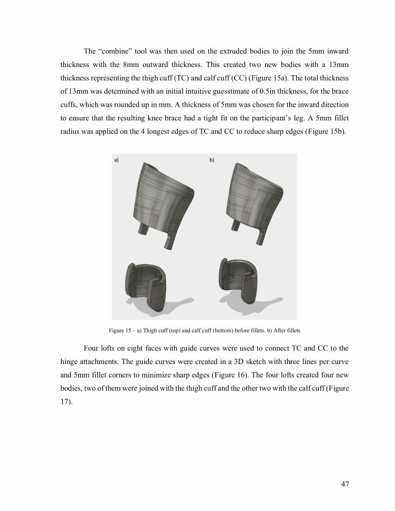
47

The “combine” tool was then used on the extruded bodies to join the 5mm inward

thickness with the 8mm outward thickness. This created two new bodies with a 13mm

thickness representing the thigh cuff (TC) and calf cuff (CC) (Figure 15a). The total thickness

of 13mm was determined with an initial intuitive guesstimate of 0.5in thickness, for the brace

cuffs, which was rounded up in mm. A thickness of 5mm was chosen for the inward direction

to ensure that the resulting knee brace had a tight fit on the participant’s leg. A 5mm fillet

radius was applied on the 4 longest edges of TC and CC to reduce sharp edges (Figure 15b).

Figure 15 – a) Thigh cuff (top) and calf cuff (bottom) before fillets. b) After fillets

Four lofts on eight faces with guide curves were used to connect TC and CC to the

hinge attachments. The guide curves were created in a 3D sketch with three lines per curve

and 5mm fillet corners to minimize sharp edges (Figure 16). The four lofts created four new

bodies, two of them were joined with the thigh cuff and the other two with the calf cuff (Figure

17).

48

Figure 16 - Eight faces used to make the four lofts are outlined in magenta and the 3D sketch guide curves are in blue.

Figure 17 – Brace cuffs combined with the 4 bodies created by the lofts gives the cuffs with complete sidebars

After the cuffs were completed, the slots needed to attach the straps were created. A

side sketch was created, and the outline of the knee brace template was included. The slots

were 5mm wide and 35mm long. They were oriented parallel to the line segments (sketch1)

and positioned 7mm from the edge of the template (Figure 18). The “extrude-cut” tool was

used on the slot sketch creating the slots in the cuffs.

49

Figure 18 - Side sketch of slot holes. All dimensions are in mm.

Next, holes in the cuffs needed to be cut out at the EMG sensor locations in accordance

with the SENIAM guidelines [165]. The rectus femoris EMG was located at 50% on the line

from the anterior spina iliaca superior of the pelvis to the superior aspect of the patella. The

gastrocnemius medialis EMG was placed on the most prominent bulge of the muscle. The

gastrocnemius lateralis EMG was placed at 1/3 of the line between the head of the fibula and

the calcaneus. For the thigh cuff, there was only one hole created for the rectus femoris

quadriceps muscle. A plane was created using the “Plane at Angle” tool on the thigh line

segment (sketch1) with an angle of 0º. A sketch was created on the plane, and a rectangle was

drawn. The rectangle dimensions were based on the size of wireless, bipolar surface EMG

electrodes (16-channel Trigno, Delsys, Boston, USA). Sketch fillets (10mm radius) were

created on the rectangle’s corners to minimize sharp edges. The “extrude-cut” tool was used

on the sketch to create a hole (Figure 19). For the calf cuff one hole for each gastrocnemius

muscle belly was created. To create the gastrocnemius holes, the shank segment line was

projected on the side plane. Then the “Plane at Angle” tool was used on the projected line to

create two planes. An angle of -30º was used for the gastrocnemius medialis plane and an

50

angle of 45º was used for the gastrocnemius lateralis plane. These plane angles guide the

hole’s sketch cutting directions and were determined visually by trial and error. A rectangle

sketch with corner fillets was created on each plane. The “extrude-cut” tool was used on the

sketches to cut through the calf cuff and create the holes (Figure 20).

Figure 19 - Rectus femoris EMG hole

51

Figure 20 - Gastrocnemius medialis and lateralis EMG holes

Once the necessary holes were created the finishing step was to fillet all remaining

sharp corners and edges. For the strap slots, a 2mm edge fillet was used. For the sensor holes

edge fillets of 5mm were used. Once the last fillets were completed the brace cuffs were ready

to be printed (Figure 21).

52

Figure 21 - Brace cuffs ready for additive manufacturing

53

3.4 3D Printing Method

Once the knee brace design was completed the parts were exported as STL files. An

Ultimaker Extended 2+ was used for 3D printing and the Cura software generated the GCODE

file. As the current knee brace design cannot be printed in one print job, there were four

separate print jobs to print the full brace. There was one print job for each hinge (right and

left), one for the TC and one for the CC. For each print job the STL files were imported into

the Cura software.

3.4.1 Orientation

The TC and CC were oriented to have the side bars pointing up and the bottom face

flat on the printer bed (Figure 22). To print the hinges, one STL file for each part was imported

and all the parts were oriented flat on the bed with the smallest bounding box dimension in

the Z direction (Figure 23).

Figure 22 - Top, thigh cuff orientation. Bottom, calf cuff orientation

54

Figure 23 - Right hinge print orientation

These orientations minimized the use of support material. For the hinges, this

orientation also corresponded to the layer orientation which should produce the strongest gear

teeth profile (primary axis of anisotropy). Due to size constraints, the TC and CC print layer

orientation was not optimal for mechanical strength. The layers are close to their weakest

orientation to resist bending stress on the sidebars. To account for this deficit other parameters

were changed.

3.4.2 Printing Parameters

All parts had the following parameter settings: wall thickness of 3.2mm, top/bottom

thickness of 2mm, and a layer height of 0.1mm. The hinges were printed with a 100% infill

parameter. TC and CC were printed with a 90% 5-step gradual infill. The gradual infill is

implemented for high infill density in the side bars and low infill density in the band section.

All other parameters were left at default. The wall and top/bottom thickness were higher than

default settings to increase the strength of the model. The infill parameters were higher to

increase the rigidity of the model. The 2nd smallest layer height was selected because the

smallest one (0.06mm) increased printing times impractically.

55

Figure 24 – Cura hinge print job parameter settings

The printed parts were removed once printing was completed and the printer bed was

cooled. The support structures were broken off with pliers. If small sharp edges remained after

removing the support structures, a file was used to smooth out any remaining sharp edges.

3.4.3 Material

The material used for the functional prototypes was a reinforced polylactic acid (PLA)

plastic named APLA+ [171]. It was chosen because it was advertised as having higher impact

and tensile strength than ABS making it appropriate for functional prototyping.

3.4.4 Assembly

To assemble the brace 12 screws (Phillips Rounded Head Thread-Forming Screws for

Plastic, 18-8 Stainless Steel, Number 0 Size, ¼” Long) were used. Each hinge required two

screws for assembly and another four screws per hinge were required to assemble the hinges

with the cuffs. Small holes in the design marked the location for the screws as described in a

previous section (see Design 2: Polycentric 1 – Spur Gears). Velcro brace straps were then

added to the 3D printed knee brace. The fitting of the knee brace was done by simply placing

the brace on the leg, with the curvature of the cuffs making the fitting intuitive. However, it

is important to check that the hinges do not restrain proper movement of the leg. A few sitting

56

knee flexion/extensions cycles and gait cycles were done with the brace on to confirm that the

fit is proper.

3.5 Prototyping

Custom functional prototypes were manufactured for 2 participants: 1) (age 46, weight

82kg, height 180cm) and 2) a female (age 24, weight 53.5kg, height 163cm). For the male

and female participants total print time and material costs were 142hrs38mins, 37.61 CAD

and 107hrs50mins, 31.00 CAD respectively. The participants were asked to self-fit their

custom brace. Minor fitting adjustments were required based on verbal feedback on comfort

and skin pressure.

3.5.1 Prototype 1

The male participant wore the brace over pants for a full day with no reported

discomfort or skin irritation. Unfortunately, the thigh cuff was not properly staying in place.

During full extensions, the superior region of the thigh cuff was falling anteriorly creating a

gap between the thigh and the brace. The weight of the thigh cuff was not held properly

because the top strap was placed too low on the thigh cuff which allowed it to fall anteriorly.

To correct this design flaw, the top strap hole needed to move superiorly. This change was

implemented in the second prototype (female) and as a result, the second prototype did not

fall anteriorly and stayed in place properly.

Another prototype experiment was performed by designing the first prototype custom

brace with a mechanical handicap; the hinges were positioned at different frontal plane angles.

This misalignment put the mechanism under higher (tension, bending, shear, torsion) loads

resulting in an accelerated failure (fatigue). This eventually (~6 months) revealed mechanical

weaknesses of the printed hinge. The first signs of failure were noted at 1 month. After ~100

cycles (one full day + intermittently/sporadically up to 3 months) of wearing, subsequent

flex/ext cycles were applied by hand on the prototype. The manual cycles consisted of

swinging the thigh cuff to swing the shank cuff in a pendulum motion. The shank cuff swung

until impact with the hinge occurred at the flex/ext brace limit (10 degrees from full

extension). These cycles started with low intensity and increased until complete mechanical

57

failure occurred (>1000 cycles). The hinge design failed before any apparent damage to the

cuffs occurred. The failure happened on the stopper at the base of the cylindrical pin and

appears to be caused by bending stress (fatigue). The misalignment caused frontal plane

bending and the thread forming screws caused assembly pretension. The printed layers were

pulled apart by the pre-tension and bending stress which accelerated the failure.

To fix the design flaws discussed above, another hinge was designed which

incorporated self-locking snap-fit features [172] removing the need for thread forming screws.

An undergraduate student (Hilal Erdogan; Faculty of Engineering, University of Copenhagen)

was tasked to create it and implemented another improvement (idea originating from Dr.

Daniel Benoit) which was to change to a herringbone gear design. It was hypothesized that it

would make the assembled hinge stronger by distributing the frontal and transverse bending

stress to the gear teeth.

The same Ultimaker Extended 2+ desktop 3D printer with the same thermoplastic

material (3D Printing Method) was used to print the parts. Print time and material cost were

8hrs41mins and 2 CAD. Thermoplastic material softens with temperature therefore the hinges

were placed in hot water to facilitate the snap fit assembly (reduce assembly forces). A

possible positive effect of the water heating process is a reheating of the layers which can

create a better bond between the printed layers therefore improving the mechanical

strength/behavior of the parts (i.e.: the plastic is annealed with hot water) [169]. The

assembled hinge was then cooled in room temperature which takes about 2mins. After

assembly these hinges were placed under manual bending load (Figure 25). Several

individuals from inside and outside of the lab were asked to break the hinge using the manual

bending method (Figure 25) and none were successful. Mechanical bending tests with a

material testing machine (i.e.: Instron) are needed to better assess the mechanical strength of

this new and improved design.

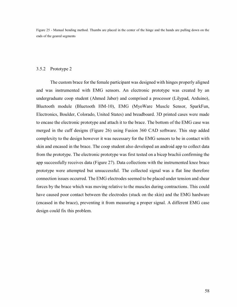
58

Figure 25 - Manual bending method. Thumbs are placed in the center of the hinge and the hands are pulling down on the

ends of the geared segments

3.5.2 Prototype 2

The custom brace for the female participant was designed with hinges properly aligned

and was instrumented with EMG sensors. An electronic prototype was created by an

undergraduate coop student (Ahmed Jaber) and comprised a processor (Lilypad, Arduino),

Bluetooth module (Bluetooth HM-10), EMG (MyoWare Muscle Sensor, SparkFun,

Electronics, Boulder, Colorado, United States) and breadboard. 3D printed cases were made

to encase the electronic prototype and attach it to the brace. The bottom of the EMG case was

merged in the cuff designs (Figure 26) using Fusion 360 CAD software. This step added

complexity to the design however it was necessary for the EMG sensors to be in contact with

skin and encased in the brace. The coop student also developed an android app to collect data

from the prototype. The electronic prototype was first tested on a bicep brachii confirming the

app successfully receives data (Figure 27). Data collections with the instrumented knee brace

prototype were attempted but unsuccessful. The collected signal was a flat line therefore

connection issues occurred. The EMG electrodes seemed to be placed under tension and shear

forces by the brace which was moving relative to the muscles during contractions. This could

have caused poor contact between the electrodes (stuck on the skin) and the EMG hardware

(encased in the brace), preventing it from measuring a proper signal. A different EMG case

design could fix this problem.

59

Figure 26 - Computer assisted-design of Prototype 2. The EMG sensor case is merged with the brace cuffs.

60

Figure 27 - Bicep brachii muscle EMG signals collected with the electronic prototype.

61

4 Validation Study – Smartphone Photogrammetry

4.1 Methods 4.1.1 Experimental Design and Data Collection

Two males (age: [26, 25], weight: [70, 118] kg, height: [175, 208] cm, BMI: [22.9,

27.3]) and two females (age: [21, 24], weight: [50, 53] kg, height: [163, 163] cm, BMI: [18.8,

19.9]) who previously suffered a knee injury were recruited via convenience sampling method

(male 2 and female 2 were ACL injuries). The participants were chosen to represent the

demographic of young adult athletes who suffered from sport-related knee injuries across a

large range of body sizes (BMI: 18.8 – 27.3).

Before scanning, four clusters of three plastic coins were placed on the limb of interest;

one distal cluster and one proximal cluster for both the thigh and the shank (Figure 28). Each

cluster defined a plane used to facilitate precise cropping of the 3D scans. The proximal thigh

cluster consisted of three coins placed on the anterior, medial and lateral proximal regions of

the thigh at 20% of the thigh length (greater trochanter to distal lateral femoral condyle). The

distal thigh cluster consisted of two coins on the femoral epicondyle landmarks and one

marker on the patella. The proximal shank cluster consists of coins on the fibula head and

anterior and medial tibia plateau landmarks. The distal shank cluster consists of two markers

on the lateral and medial malleoli and one above the heel on the Achilles tendon.

Scans of the injured legs were created using two methods. The first method used the

low-cost 3D scanner (iSense; criterion) and the second used the developed smartphone

photogrammetry procedure. An iPhone 6S was used which has a 12 mega-pixel (MP) camera.

Three researchers (observers/raters), were graduate students from the University of Ottawa,

were trained to perform the data collection. The individual training consisted of three practice

scans with instructions and feedback with corrections for each researcher. Each participant

was scanned during separate sessions. Each researcher performed three scans of each

participant with each device. This resulted in 18 scans per session for a total of 72 scans (4

participants x 3 researchers x 3 repetitions x 2 devices). The researcher sequence and the

device sequence were performed in a randomised order with minimal break between each

scan.

62

Figure 28 – Frame extracted from the video recording. Plastic coins on the leg were used to aid in mesh reconstruction and

processing

4.1.2 Data Processing

The 3D scans we’re manually cropped using Autodesk Recap (see Mesh Processing).

The proximal and distal plane used for cropping passed by the edges of the three markers in

their respective cluster (Figure 29). Next, the 3D mesh was transformed into a 3D body by

closing all remaining holes. The resulting body was exported as a PLY file which was then

imported into the open source software MeshLab (Istituto di Scienza e Tecnologie

63

dell’Informazione, Pisa, Italy). All the scans from one participant were imported into one

Meshlab project and were aligned with the rigid point cloud registration filter before extracting

measurements.

Figure 29 – Cropped leg showing the proximal (thigh) and distal (ankle) clusters used for cropping.

The following measurements were extracted for all scans: Hausdorff Distances between

each pair of repeated scans, total limb volume, limb bounding box size (BBox), knee joint

center (KJC) coordinates and 15 cross-sectional areas (CSA) for the thigh and the shank. The

knee joint center was defined as the midpoint of the line connecting the femoral epicondyle

markers [173] and serves as a critical landmark used in the digital orthopedic alignment

process of the custom knee brace design (see Digital Alignment & Brace Cuff Design). The

coordinates of both femoral epicondyle landmarks were extracted manually for all scans by

selecting the surface point closest to the center of the plastic coins (determined visually based

on the color texture of the 3D body) and saving the x,y,z coordinates in Meshlab log files. The

rest of the measurements were extracted using a custom Python script which also computed

the statistical analysis (see Python Scripts). The CSA for the shanks were spaced equidistantly

starting from the anterior tibia plateau over the gastrocnemius muscle belly and stopping

64

before the ankle malleoli landmarks. The thigh CSA were also spaced equidistantly starting

from the femoral epicondyle landmarks and covering the entire thigh. The limb bounding box

was defined as the smallest box that contains the whole limb geometry in the x,y and z axes.

4.1.3 Statistical Analysis

Accuracy and precision (validity and reliability) of the smartphone scanning procedure

were assessed using the statistical approach suggested by Hopkins [174]. This well-

established analysis is used to quantify measurement agreement between two measurement

methods. It consists of calculating the measurement differences between the two methods,

calculating the mean bias and 95% limits of agreement (LoA) of the differences. For the

accuracy assessment, the iSense sensor was considered the criterion and the smartphone was

considered as the practical measurement system. For the precision assessment inter-rater and

intra-rater analyses were performed. The data were organized in three groups (one for each

scan repetition) for the intra-rater analysis. For the inter-rater analysis the data were organized

in another three groups (one for each rater). The following variables were calculated with a

95% Confidence Interval (CI) for all variables: change in the mean (the mean difference

between the repeated scan results), typical error of the measurements (TEMs) and Intra-class

Correlation Coefficients (ICC(3,1)) [175]. The intra and inter-rater variability was calculated

as 1.96√2 𝑇𝐸𝑀𝑠 following the Bland-Altman method [176] and as reported in reliability

studies for residual limb geometry [176]–[178]. ICC values between 0.75 and 0.9 were

considered good reliability and values greater than 0.9 were considered excellent reliability

[179]. HD mean and BBox values for change in the mean, TEMs and intra/inter-rater

variability below 20mm were considered good and above were considered bad (see Design

Requirements). KJC values for change in the mean, TEMs and intra/inter-rater variability

below 5mm were considered good and above were considered bad (see Design Requirements).

4.2 Results The measured limb volumes ranged from 4088 ml to 11378 ml (Table 1). The maximum

Hausdorff Distance ranged from 30.2 mm to 73.9 mm or 4.37 % to 8.79 % of their mesh’

bounding box diagonal. The largest mean Hausdorff Distances ranged from 6.8 mm to 11.2

mm (0.98 % to 1.61 %).

65

Table 1 - Participant overall measurements. HD = Hausdorff Distance

Female 1 Female 2 Male 1 Male 2

BMI [kg/m2] 18.8 19.9 22.9 27.3

Mean Volume [ml] 4762.5±565.6 6713.8±571.0 6394.7±477.4 10005.8±669.7

Max HDMax [mm] 47.3 30.2 41.0 73.9

Max HDMax [%] 6.73 4.37 5.68 8.79

Mean HDMax [mm] 11.2 6.8 7.7 10.9

Mean HDMax[%] 1.61 0.98 1.07 1.29

4.2.1 Validity

Bland-Altman plots show that the smartphone photogrammetry method

underestimated the limb volume by approximately 600 ml compared to the iSense sensor

(Figure 30). This bias corresponded to 11% of the actual volumes. A clear separation of the

data showed that the four chosen participants cover a large range of body sizes (BMI range:

18.8 – 27.3). The cluster on the right side of the graph represents the participant “Male 2” with

a mean volume of 10005.8 ± 669.7 ml. The participants “Female 2” and “Male 1” have similar

volumes (6713.8 ± 571.0 ml and 6394.7 ± 477.4 ml respectively) and are clustered together

in the middle. The “Female 1” participant has a mean volume of 4762.5 ± 565.6 ml and is also

clearly separated from the other participants.

The participant “Male 2” has the largest spread (absolute and percentage) and is the

only one with overestimated values. This outlier ultimately affected the 95% limits of

agreement to be large (around 1.5L). The other three participants have similar absolute spread

however the percentage(relative) spread for “Female 1” is more pronounced due to a smaller

volume average.

66

Figure 30 - Bland-Altman plot of the volume measurements. Top is the absolute difference between the smartphone

photogrammetry and the iSense sensor. Bottom is the error of the smartphone volume measurements expressed as a

percentage of the volume average. A negative value represents that the smartphone underestimates the volume with respect

to the iSense sensor. The solid lines represent the mean of the differences and the mean of the errors. The dashed lines

represent the upper and lower 95% limits of agreement.

67

Figure 31 – Bland-Altman plots for the cross-sectional area (CSA) measurements of the thigh. Top is the absolute difference

between the smartphone photogrammetry and the iSense sensor. Bottom is the error of the smartphone measurements

expressed as a percentage of the average. A negative value represents that the smartphone underestimates the CSA with

respect to the iSense sensor. The solid lines represent the mean of the differences and the mean of the errors. The dashed

lines represent the upper and lower 95% limits of agreement.

The Bland-Altman plots for the cross-sectional areas (CSA) also revealed that the

smartphone method underestimated the limb geometry. For the thigh portion, the magnitude

of the absolute difference was around -9 cm2 or around -8% of the CSA average (Figure 31).

For the shank portion the magnitude of the absolute difference was around -11 cm2 or around

-15% of the CSA average (Figure 32). Additionally, for both the thigh and shank CSA the

difference increased with the average. The larger CSA were mostly overestimated which was

reflective of the “Male 2” volume overestimations.

68

Figure 32 - Bland-Altman plots for the cross-sectional area (CSA) measurements of the shank. Top is the absolute difference

between the smartphone photogrammetry and the iSense sensor. Bottom is the error of the smartphone measurements

expressed as a percentage of the average. A negative value represents that the smartphone underestimates the CSA with

respect to the iSense sensor. The solid lines represent the mean of the differences and the mean of the errors. The dashed

lines represent the upper and lower 95% limits of agreement.

The bounding box size measurements (i.e. anterior-posterior, medial-lateral and

proximal-distal) also confirmed the underestimation of the smartphone method relative to the

iSense sensor with the largest bias of -7.4 mm in the anterior-posterior axis. The KJC

coordinates had bias values < 5mm for the anterior-posterior and medial-lateral axis however

for the proximal-distal the bias was 6.8 mm (Table 2).

69

Table 2 - Validity Results. BBox = Bounding Box measurements, Ant-Post = anterior-posterior axis, Med-Lat = medial-lateral axis, Prox-Dist = proximal-distal axis, KJC = knee joint center coordinates.

Overall Bias Limits of Agreement

Absolute Relative

(%)

Absolute Relative

(%)

Pearson

CC

CV

(%)

BBox

Ant-Post

(x)

-7.4

(-10.9; -3.9) mm

0.97

(0.69; 1.38)

20.3

mm

7.52 0.90 3.59

Med-Lat

(y)

-3.4

(-7.3; 0.5) mm

0.98

(0.68; 1.40)

22.8

mm

7.91 0.86 4.08

Prox-Dist

(z)

-0.5

(-2.8; 1.7) mm

1.00

(0.71; 1.40)

13.2

mm

7.11 1.00 1.00

KJC

Ant-Post

(x)

-3.3

(-5.2; -1.3) mm

- 11.5

mm

- 0.99 -

Med-Lat

(y)

2.0

(0.8; 3.1) mm

- 6.8

mm

- 0.94 -

Prox-Dist

(z)

6.8

(4.2; 9.3) mm

- 14.9

mm

- 1.00 -

Volume -589.0

(-858.5; -319.5)

ml

0.90

(0.62; 1.30)

1561.4

ml

8.78 0.96 5.82

4.2.2 Reliability

The smartphone photogrammetry method showed good levels of intra- and inter-rater

reliability with ICCs greater than 0.90 (Table 3 and Table 4). The TEMs were below 5% for

the bounding box and volume measurements and < 3mm for the KJC coordinates. The KJC

coordinates showed the best inter- and intra-rater reliability coefficients which were < 5mm

for the anterior-posterior and medial-lateral axis however for the proximal-distal axis they

were over 6mm similar to the overall bias from the validity analysis.

70

Table 3 - Intra-rater reliability results. BBox = Bounding Box measurements, Ant-Post = anterior-posterior axis, Med-Lat =

medial-lateral axis, Prox-Dist = proximal-distal axis, KJC = knee joint center coordinates.

Typical Error of Measurement

Change In Mean Absolute Relative (%) Reliability ICC

BBox

Ant-Post (x)

-2.1 (-9.6; 5.3) mm 8.3 (6.2; 12.4) mm

3.07

(2.30; 4.63) 22.9 mm 0.90

Med-Lat (y)

-0.9 (-6.7; 4.9) mm 6.5 (4.9; 9.7) mm

3.39

(2.54; 5.12) 18.0 mm 0.92

Prox-Dist (z)

-1.7 (-5.8; 2.3) mm 4.7 (3.5; 7.0) mm

0.79

(0.59; 1.18) 13.0 mm 1.00

KJC

Ant-Post (x) -0.6 (-2.1; 0.9) mm 1.7 (1.3; 2.6) mm - 4.8 mm 1.00

Med-Lat (y) -0.4 (-1.5; 0.7) mm 1.2 (0.9; 1.8) mm - 3.4 mm 0.96

Prox-Dist (z) -0.2 (-2.3; 1.8) mm 2.2 (1.7; 3.4) mm - 6.2 mm 1.00

Volume -228.9

(-565.3; 107.5) ml

375.3

(281.9; 561.3) ml

4.77

(3.56; 7.21) 1040.2 ml 0.98

Table 4 - Inter-rater reliability results. BBox = Bounding Box measurements, Ant-Post = anterior-posterior axis, Med-Lat =

medial-lateral axis, Prox-Dist = proximal-distal axis, KJC = knee joint center coordinates.

Typical Error of Measurement

Change In Mean Absolute Relative (%) Reliability ICC

BBox

Ant-Post (x)

1.0 (-5.4; 7.3) mm 7.4 (5.6; 11.1) mm

2.74

(2.05; 4.12) 20.6 mm 0.92

Med-Lat (y)

0.4 (-4.9; 5.8) mm 5.9 (4.5; 8.9) mm

3.07

(2.30; 4.63) 16.5 mm 0.94

Prox-Dist (z)

0.8 (-2.8; 4.3) mm 4.0 (3.0; 5.9) mm

0.66

(0.5; 0.99) 11.0 mm 1.00

KJC

Ant-Post (x) -0.5 (-2.1; 1.1) mm 1.7 (1.3; 2.6) mm - 4.8 mm 1.00

71

Med-Lat (y) 0.2 (-1.0; 1.4) mm 1.3 (1.0; 2.0) mm - 3.7 mm 0.95

Prox-Dist (z) 0.4 (-1.7; 2.5) mm 2.3 (1.7; 3.5) mm - 6.4 mm 1.00

Volume 48.6

(-238.7; 335.9) ml

320.8

(241.0; 479.8) ml

3.56

(2.66; 5.37) 889.14 ml 0.98

4.3 Discussion

This study assessed the validity and reliability of a novel low-cost 3D scanning method

(versus the previously validated iSense sensor [38]) for the leg with a wide range of body

sizes. This investigation was the first to provide validity, intra-rater and inter-rater reliability

analysis for smartphone photogrammetry of human body leg geometry. Validity and reliability

are important to determine the accuracy of new measurement methods, the quality of the data

and if they are appropriate for clinical applications [180].

The study was designed to reflect sub-optimal but realistic results obtained with the

developed smartphone photogrammetry procedure. As such, an iPhone 6S smartphone with a

12MP camera was used as the data collecting device. This was far from being the best

smartphone camera available for the same price [181]. A higher MP count provides more data

for the reconstruction algorithms and could drastically improve the results.

Dessery and Pallari [38] investigated the measurement agreement between the iSense

sensor and a high-level 3D scanner (Artec EVA) for knee geometry. The iSense sensor showed

to overestimate the circumference with a mean bias of 13mm (0.88%) and LoA from 1.4 to

24.8mm (-0.1% to 1.86%). Interestingly, the results from the smartphone photogrammetry

method underestimated the iSense sensor for the volume and bounding box size measurements

by 0.90 to 1.0 % and LoA from 7.11 to 8.78%. The larger LoA were a result of “Male 2”

significantly affecting the analysis and therefore was representative of an outlier from large

body sizes. The weight and height of Male 2 was 118kg and 208cm respectively while the

average weight and height for US males between 20-29 years old is 84.7kg (90th percentile =

113.3kg, 95th percentile = 124.9kg) and 176.4cm (95th percentile = 188.8cm) respectively

[182]. In practice, such body sizes would require adding an additional step to the smartphone

photogrammetry method such as taking the mean of multiple scans or performing a different

regression prediction. Unfortunately, this study did not report any circumference measurement

72

since the chosen free software did not reveal to have the necessary tools. However, the CSA

measurements are a similar measurement and were also showing underestimation.

Additionally, the low participant sample size is a limitation of this study. The developed

workflow is targeted to late-teen pediatric populations and early adult populations. These

populations were found to have a higher number of ACL knee injuries than mid-teens [183].

In this study, the sample population comprised of four young adult athletes of which Female

1 was considered to be representative of the late-teens pediatric populations and the other three

were representative of the early adult populations. Although only four participants were

recorded, two of the body sizes reported (female 1 BMI: 18.8, male 2 BMI: 27.3) represented

close to the 5th and 95th percentiles for 20-29 year old US athletes (males: 18.29 and 28.96,

females: 17.58 and 25.67) [184]. This could explain the relatively large LoA and it is

reasonable to expect that a study with a larger sample size would show LoA closer to what

was previously reported [38], [39]. Nonetheless the underestimation of the smartphone

photogrammetry method suggests that it could reveal to be closer to the Artec EVA than the

iSense sensor. With a 15.1 MP camera, the theoretical accuracy of a photogrammetry system

is thought to be around 0.05 mm [151]. In practice reaching such measurement accuracy also

relies on the 3D reconstruction algorithm and proper lighting. For this study, the free version

of Autodesk Recap is the photogrammetry software used which limited the number of photos

to 100. The paid version which allows up to 1000 photos would likely reveal to have better

results.

The data collection location for the study was indoors where the only lighting came

from ceiling lights. Figure 33 shows the HD as a color map (red means 0 and blue means >

5mm) for the two 3D meshes with the smallest mean HD obtained using the smartphone

method (Male 1). The frontal view shows mostly red and yellow colors (0 – 1.5mm) while the

rear view has a lot of green and some blue (2mm – 5mm). This clear contrast was very similar

to the lighting contrast that was present during the smartphone photogrammetry procedure

(Figure 3). It shows that the sub-optimal lighting clearly affected even the best results

therefore it was likely a large contributor to measurement error. This was a good example that

supports the necessity to have good, even and consistent lighting for successful

photogrammetry as previously reported [150], [162]–[164].

73

Despite these sub-optimal conditions for the photogrammetry method, the anterior-

posterior and medial-lateral KJC coordinates revealed to have overall absolute bias and

reliability coefficients below the 5mm design requirement (Design Requirements). This

requirement comes from a study [45] which showed large changes in the mechanics (forces

and joint contact errors) due to only 5mm of anterior misplacement. The study also showed

that anterior-posterior misplacement had the highest change and the proximal-distal

misplacement is attributed with the least change.

Figure 33 - Hausdorff distance color map of the two best scans obtained with the smartphone photogrammetry method. The

left side shows the Hausdorff distance distribution in cm. Red means 0 distance and blue means the distance is > 5mm.

74

5 Conclusion and Future Work

5.1 Summary

This thesis provided the foundational work for a low-cost 3D printed custom knee brace.

Specifically, the research, development and implementation of a novel workflow aimed to be

easy to use and available to anyone who has access to a smartphone camera and 3D printing

services. Our scanning method provides limb geometry results that are suitable for this

application. The validation study was an explorative pilot study and the results can be used to

guide the design of a larger study. This study should be repeated on a larger sample size with

late-teens and early adults [183]. This sample could reveal to have a body size mean

distribution closer to “Female 2” and “Male 1” which were the body sizes with the best results.

The results could impact the decision regarding clinical use of the smartphone

photogrammetry method.

The developed workflow was used to manufacture two prototypes which helped in the

design iterations. As a result, an improved hinge was created which could reveal to have

sufficient mechanical strength for a fully 3D printed custom knee brace. The second prototype

suggested that a more conforming brace design could be more appropriate for successful EMG

data collection.

This novel methodology required little training which could be provided through video

instructions posted online. It would enable the patient to collect their own “3D scan” with the

help of a friend or family member, effectively removing the need to book an appointment

simply for collecting custom measurements. Additionally, it would allow the clinician to focus

all their time on clinically relevant design tasks such as checking alignment, fit and comfort

which could all potentially be improved by adopting digital methods. The ultimate vision is

to make better custom knee braces which are easily accessible at a reduce cost.

5.2 Recommendations/Future Work

This thesis served as a critical initial step in the development of a low-cost custom knee

brace. The smartphone photogrammetry method showed good early validation results and

supports future investigation with a larger sample size. The larger study should perform data

75

collection outside during cloudy days to reduce error from bad lighting and to investigate the

feasibility of a weather dependent method. Additionally, better accuracy and precision results

can be obtained by using a smartphone with more megapixel, the full version of Autodesk

Recap or another software such as a custom Maltab or Python script.

Regarding the design of the brace, future work should investigate optimal 3D printing

parameters including material choice, printer type and build orientation of the cuffs. A dual-

nozzle 3D printer which can use water-soluble support material would allow a wider range of

printing orientation and could be used to determine optimal mechanical strength for the brace

cuffs. Furthermore, mechanical testing of the improved hinge is needed. An Instron machine

could be used for 3-point bend testing of the hinge for medial-lateral and flexion-extension

loading scenarios. Impact testing would also be necessary before such a brace could be worn

during sports activities. Ultimately, a hinge design which has patient-specific motion

(dynamic customization) should be investigated.

While beyond the scope of this thesis, the workflow itself could be improved by

automating mesh processing and design generation. Mesh processing and landmark

detection/extraction could be automated with a machine learning algorithm that uses the 3D

shape of the leg as input. A challenging step would be to collect real-time MRI and/or X-ray

video to label the precise path of the knee joint center with respect to the exterior surface

geometry. Instead, something possibly achievable within 1-2 years would be to collect a large

number of 3D scans with the smartphone photogrammetry method and the KJC labelled (see

Data Processing). Another could use two simultaneous video recordings (i.e: sagittal and

frontal) to estimate the path of the KJC through frameworks such as OpenPose

(https://github.com/CMU-Perceptual-Computing-Lab/openpose/blob/master/doc/output.md).

The current CAD workflow uses free software which are controllable with the Python

programming language making it ideally suited for open-source community contributions.

Making such a project open-source could bring significantly more contributions in a short

amount of time allowing automation of the CAD much sooner and the impact becoming real.

Many companies have certain operations that follow open-source models (i.e. Google,

Facebook and Amazon) therefore the various types of open-source licenses should be

investigated.

https://github.com/CMU-Perceptual-Computing-Lab/openpose/blob/master/doc/output.md

77

6 Appendix

6.1 Python Scripts 6.1.1 meshlabserverPyAuto.py import os import time import numpy as np import pandas as pd import scipy.stats import matplotlib.pyplot as plt from importKJCdata import importKJCdata start = time.time() print("hello") def bland_altman_plot(data1, data2, varname, units): data1 = np.asarray(data1) data2 = np.asarray(data2) mean = np.mean([data1, data2], axis=0) diff = data1 - data2 # Difference between data1 and data2 md = np.mean(diff) # Mean of the difference sd = np.std(diff, axis=0) # Standard deviation of the difference diffperc = 100*np.divide(diff, mean) mdperc = np.mean(diffperc) sdperc = np.std(diffperc, axis=0) fig=plt.figure(figsize=(10,9)) ax1=plt.subplot2grid((2,1),(0,0),rowspan=1,colspan=1) ax1.scatter(mean, diff,s=5) ax1.axhline(md, color='gray', linestyle='-') ax1.axhline(md + 1.96*sd, color='gray', linestyle='--') ax1.axhline(md - 1.96*sd, color='gray', linestyle='--') xlabel=varname+' average '+units ylabel= varname+' difference '+units+'\n(Smartphone - Structure Sensor)' ax1.set_xlabel(xlabel) ax1.set_ylabel(ylabel) ax2=plt.subplot2grid((2,1),(1,0),rowspan=1,colspan=1) ax2.scatter(mean, diffperc,s=5) ax2.axhline(mdperc, color='gray', linestyle='-') ax2.axhline(mdperc + 1.96*sdperc, color='gray', linestyle='--')

78

ax2.axhline(mdperc - 1.96*sdperc, color='gray', linestyle='--') xlabel=varname+' average '+units ylabel= 'Mean percentage error (%)' ax2.set_xlabel(xlabel) ax2.set_ylabel(ylabel) figname=varname+'_BlandAltman.pdf' # plt.show() fig.savefig(figname) def validity (pract, crit): cl=95 # confidence limit is 95% mpract=np.mean(pract) mcrit=np.mean(crit) stdpract=np.std(pract) stdcrit=np.std(crit) N=len(pract) slope, intercept, r_value, p_value, std_err=scipy.stats.linregress(pract,crit) bias=pract-crit mbias=np.mean(bias) stdbias=np.std(bias) devsqpract= np.sum(np.square(pract - mpract)) # see definition of DEVSQ() in Excel tinv=-1*scipy.stats.t.ppf(((1-(cl/100))*0.5),N-1) biasLCL=mbias - tinv*stdbias/np.sqrt(N) biasUCL=mbias + tinv*stdbias/np.sqrt(N) LOA=1.96*stdbias r,p=scipy.stats.pearsonr(pract,crit) # relative stats logpract=100*np.log(pract) logcrit=100*np.log(crit) mlogcrit=np.mean(logcrit) mlogpract=np.mean(logpract) logbias=logpract-logcrit mlogbias=np.mean(logbias) stdlogbias=100*np.exp((1/100)*np.std(logbias))-1

79

relbias=np.exp(mlogbias/100) tinv=-1*scipy.stats.t.ppf(((1-(cl/100))*0.5),N-1) relbiasLCL=np.exp((mlogbias - tinv*stdlogbias/np.sqrt(N))/100) relbiasUCL=np.exp((mlogbias + tinv*stdlogbias/np.sqrt(N))/100) relLOA=np.exp(1.96*stdlogbias/100) y2=np.sum(np.square(logcrit-mlogcrit)) x2=np.sum(np.square(logpract-mlogpract)) xy2=np.square(np.sum(np.multiply((logcrit-mlogcrit),(logpract-mlogpract)))) steyx=np.sqrt((1/(N-2))*(y2 - xy2/x2)) # see Excel STEYX() documentation for equation typicalerrorofestimate_factor=np.exp(steyx/100) CV_perc=(typicalerrorofestimate_factor-1)*100 statsout=[mbias, biasLCL, biasUCL, relbias, relbiasLCL, relbiasUCL, LOA, relLOA, r, CV_perc] return statsout def reliability (dataset): dim=list(np.shape(dataset)) N=dim[0] nrow=dim[0] ncol=dim[1] df=N-1 cl=95 # Changes in Score changescores=np.zeros((N,ncol-1)) for i in range(ncol-1): changescores[:,i]=dataset[:,i+1]-dataset[:,i] # Change in Mean MeanOfChange=np.mean(changescores,axis=0) StdOfChange=np.std(changescores,axis=0) tinv=-1*scipy.stats.t.ppf(((1-(cl/100))*0.5),df) MeanOfChangeLCL=MeanOfChange - tinv*StdOfChange/np.sqrt(N) MeanOfChangeUCL=MeanOfChange + tinv*StdOfChange/np.sqrt(N) ChangeInMean=np.mean(MeanOfChange) ChangeInMeanLCL=np.mean(MeanOfChangeLCL) ChangeInMeanUCL=np.mean(MeanOfChangeUCL)

80

# Mean of the typical error with lower and upper confidence levels TypicalError=np.std(changescores, axis=0)/np.sqrt(2) sumproduct=np.sum(df*(np.multiply(TypicalError,TypicalError))) mTypicalError=np.sqrt(sumproduct/(df*(ncol-1))) meanDF=(1-0.22*N*ncol/(ncol*N))*df*(ncol-1) Q67=meanDF Q56=mTypicalError probability=(1-cl/100)/2 CHIINV=scipy.stats.chi2.ppf(1-probability, Q67) mTypicalErrorLCL=np.sqrt(Q67*np.power(Q56,2)/CHIINV) CHIINV=scipy.stats.chi2.ppf(1-(1-probability), Q67) mTypicalErrorUCL=np.sqrt(Q67*np.power(Q56,2)/CHIINV) #Reliability Coefficient ReliabilityC=1.96*np.sqrt(2)*mTypicalError #ICC raw data mdataset=np.mean(dataset, axis=0) stddataset=np.std(dataset, axis=0) sumproduct=np.sum(df*(np.multiply(stddataset,stddataset))) J43=np.sqrt(sumproduct/(df*ncol)) R42=nrow mICC=(1-np.power(Q56,2)/np.power(J43,2))*(1+(1-np.power((1-np.power(Q56,2)/np.power(J43,2)),2))/(R42-3)) # Relative stats logdataset=100*np.log(dataset) changescoreslog=np.zeros((N,ncol-1)) for i in range(ncol-1): changescoreslog[:,i]=logdataset[:,i+1]-logdataset[:,i] logTypicalError=np.std(changescoreslog, axis=0)/np.sqrt(2) sumproduct=np.sum(df*(np.multiply(logTypicalError,logTypicalError))) mlogTypicalError=np.sqrt(sumproduct/(df*(ncol-1))) mpercTypicalError=100*np.exp(mlogTypicalError/100) - 100 AI119=meanDF AI109=mlogTypicalError CHIINV=scipy.stats.chi2.ppf(1-probability, AI119) mlogTypicalErrorLCL=np.sqrt(AI119*np.power(AI109,2)/CHIINV) mpercTypicalErrorLCL=100*np.exp(mlogTypicalErrorLCL/100) - 100 CHIINV=scipy.stats.chi2.ppf(1-(1-probability), AI119) mlogTypicalErrorUCL=np.sqrt(AI119*np.power(AI109,2)/CHIINV)

81

mpercTypicalErrorUCL=100*np.exp(mlogTypicalErrorUCL/100) - 100 statsout=[ChangeInMean, ChangeInMeanLCL, ChangeInMeanUCL, mTypicalError, mTypicalErrorLCL, mTypicalErrorUCL, ReliabilityC, mpercTypicalError, mpercTypicalErrorLCL, mpercTypicalErrorUCL, mICC, MeanOfChange, MeanOfChangeLCL, MeanOfChangeUCL] return statsout # Example of meshlab command to run """ meshlabserver command example meshlabserver -l C:/Users/omigu094/Desktop/MeshLabScripting/Celi/ComparisonResults/log_CPB1vsCPB2.txt -i C:/Users/omigu094/Desktop/MeshLabScripting/Celi/CPB1.ply -i C:/Users/omigu094/Desktop/MeshLabScripting/Celi/CPB2.ply -s C:/Users/omigu094/Desktop/MeshLabScripting/Hausdorff_Distance.mlx -o C:/Users/omigu094/Desktop/MeshLabScripting/Celi/ComparisonResults/CPB1vsCPB2.ply -m vc vf vq vn vt fc ff fq fn wc wn wt -i C:/Users/omigu094/Desktop/MeshLabScripting/Celi/CPB1.ply -i C:/Users/omigu094/Desktop/MeshLabScripting/Celi/CPB2.ply -o C:/Users/omigu094/Desktop/MeshLabScripting/Celi/ComparisonResults/CPB1vsCPB2.ply -m vc vf vq vn vt fc ff fq fn wc wn wt -s C:/Users/omigu094/Desktop/MeshLabScripting/Hausdorff_Distance.mlx -l C:/Users/omigu094/Desktop/MeshLabScripting/Celi/ComparisonResults/log_CPB1vsCPB2.txt """ # Define project path # Lab computer # projectfolder= "C:/Users/omigu094/Desktop/MeshLabScripting/" # meshlabservercall="meshlabserver" # Olivier Macbook Pro projectfolder= "/Users/Olivier/3DAnalysisSession1/" meshlabservercall="/Applications/meshlab.app/Contents/MacOS/meshlabserver"

82

outputfolder= projectfolder+"MeshLabLogResults/" filterfolder=projectfolder+"Filters/" inputfolder=projectfolder+'MeshesSolid/' # Define scripts to be used hausmlxscriptfilename = filterfolder+"HausdorffDistance_ColorizebyVertexQuality.mlx" geomlxscriptfilename = filterfolder+"GeoMeasures.mlx" # full lists of file categories subjectList = ["Lisa","Celi","Mike","Nick"] deviceID = ["P", "S"] partList = ["B", "La","Lu"] # test lists # subjectList = ["Lisa"] # partList = ["B"] # deviceID = ["P"] trials=[1,2,3] # Scans metadata nscans=len(partList)*len(deviceID)*len(trials) nsub=len(subjectList) fileIDList=[[None]*nscans for i in range(nsub)] # List of variables that are outputted. Currently only works with the Hausdorff Distance variable dataoutlist=["HauDisMaxCent","HauDisMaxPerc","HauDisMeanCent","HauDisMeanPerc"] # Trying to use "dictionary" to define the variables. This way to whole code can be looped through the dictionary and run the same stuff for all variables in the dictionary """ vardict={} for item in dataoutlist: vardict[item]=np.zeros(shape=(nsub,nscans,nscans)) """ # Mesh variables HauDisMaxCent=np.zeros(shape=(nsub,nscans,nscans)) HauDisMaxPerc=np.zeros(shape=(nsub,nscans,nscans)) HauDisMeanCent=np.zeros(shape=(nsub,nscans,nscans)) HauDisMeanPerc=np.zeros(shape=(nsub,nscans,nscans)) BBoxSize=np.zeros(shape=(nsub,nscans,3))

83

SurfArea=np.zeros(shape=(nscans,nsub)) Volume=np.zeros(shape=(nscans,nsub)) # Cross section surface area variables planeZsections=[np.arange(25,40),np.arange(25,40),np.arange(-10,5),np.arange(35,50)] planeCsections=[np.arange(33,48),np.arange(30,45),np.arange(9,24),np.arange(58,73)] nsect=30 CrossSurfArea=np.zeros(shape=(nsub,nscans,nsect)) list_trialID=[] # Creates a list containing the mesh file names without the extension for s,subject in enumerate(subjectList): n=0 for device in deviceID: for participant in partList: for trial in trials: fileIDList[s][n] = subject[0]+device+participant+str(trial) if s==0: list_trialID=list_trialID+[device+participant+str(trial)] n=n+1 # Runs through all the files and extracts the values for the variables defined above for s,subject in enumerate(subjectList): for t,targetFileID in enumerate(fileIDList[s]): targetfilename = inputfolder+targetFileID+".ply" # target file targetfileinputcmd = " -i "+targetfilename # This block runs "Compute Planar Section" and "Compute Geometric Measures" filters to extract the CrossSurfArea from 15 slices of the tibia and thigh for each file for z,sect in enumerate(planeZsections[s]): logfilename = outputfolder+targetFileID+"LOG_PlanarSectionGeoMeasuresZ"+str(sect)+".txt" logfilecmd = " -l "+logfilename planesectmlxscriptname=filterfolder+'PlanarSection_GeoMeasure_Z_'+str(sect)+'_mesh.mlx' mlxscriptcmd = " -s "+planesectmlxscriptname meshlabservercmd=meshlabservercall + logfilecmd + targetfileinputcmd + mlxscriptcmd #os.system(meshlabservercmd)

84

with open(logfilename) as file: data = file.readlines() CrossSurfAreaLine=data[8].split() CrossSurfArea[s][t][z]=float(CrossSurfAreaLine[4]) for c,sect in enumerate(planeCsections[s]): if s==2: caxes="(-0d7_0_1)_" elif s==3: caxes="(-0d5_0_1)_" else: caxes="(1_0_1)_" logfilename = outputfolder+targetFileID+"LOG_PlanarSectionGeoMeasuresC"+caxes+str(sect)+".txt" logfilecmd = " -l "+logfilename planesectmlxscriptname=filterfolder+"PlanarSection_GeoMeasure_C"+caxes+str(sect)+"_mesh.mlx" mlxscriptcmd = " -s "+planesectmlxscriptname meshlabservercmd=meshlabservercall + logfilecmd + targetfileinputcmd + mlxscriptcmd #print(meshlabservercmd) # os.system(meshlabservercmd) with open(logfilename) as file: data = file.readlines() CrossSurfAreaLine=data[8].split() CrossSurfArea[s][t][z+c+1]=float(CrossSurfAreaLine[4]) # This block runs the "Compute Geometric Measures" filter on all the scans logfilename = outputfolder+targetFileID+"_GeoMeasures.txt" logfilecmd = " -l "+logfilename mlxscriptcmd = " -s "+geomlxscriptfilename meshlabservercmd=meshlabservercall + logfilecmd + targetfileinputcmd + mlxscriptcmd # run the command # os.system(meshlabservercmd) with open(logfilename) as file: data = file.readlines() BBoxSizeLine=data[3].split() # line containing BBoxSize data in cm BBoxSize[s][t]=[float(BBoxSizeLine[4]), float(BBoxSizeLine[5]),float(BBoxSizeLine[6])]

85

SurfAreaLine=data[7].split() SurfArea[t][s]=float(SurfAreaLine[4]) VolumeLine=data[12].split() Volume[t][s]=float(VolumeLine[3]) # temporary block to remove colors ''' outputfolder=projectfolder+'MeshesNoColor/' outputfilecmd=" -o " + outputfolder + targetFileID + ".ply" meshlabservercmd=meshlabservercall + targetfileinputcmd + outputfilecmd os.system(meshlabservercmd) ''' # This loop computes the Hausdorff distance filter between all the files for each subject for sam,sampledFileID in enumerate(fileIDList[s]): mlxscriptcmd = " -s "+hausmlxscriptfilename sampledfilename = inputfolder+sampledFileID+".ply" #sampled file sampledfileinputcmd = " -i "+sampledfilename logfilename = outputfolder+"log_"+targetFileID+"vs"+sampledFileID+".txt" logfilecmd = " -l "+logfilename outputfilecmd=" -o " + outputfolder + targetFileID + "vs" + sampledFileID + ".ply -m vc vf vq vn vt" # full command #print('sam='+sampledfilename) #print('t='+targetfilename) meshlabservercmd=meshlabservercall + logfilecmd + sampledfileinputcmd + targetfileinputcmd + mlxscriptcmd + outputfilecmd # run the command # os.system(meshlabservercmd) with open(logfilename) as file: data = file.readlines() cmLine=data[7].split() # line containing data in cm HauDisMaxCent[s][t][sam]=float(cmLine[4]) HauDisMeanCent[s][t][sam]=float(cmLine[7]) percLine=data[9].split() # line containing data in perc HauDisMaxPerc[s][t][sam]=float(percLine[4]) HauDisMeanPerc[s][t][sam]=float(percLine[7]) # # testing command outside looping # os.system(meshlabservercmd)

86

# print(type(meshlabservercmd), len(meshlabservercmd)) # print(meshlabservercmd) # print(data) # Calculate min and max values for Hausdorff Distances for each subject for s in range(len(subjectList)): a=HauDisMeanCent[s][:][:] minval = np.min(a[np.nonzero(a)]) maxval = np.max(a[np.nonzero(a)]) # Here the data in the variables are written in text files for human verification #Write CrossSurfArea (CSA) data into txt file outfilename=outputfolder+'CSA.txt' with open(outfilename, 'wb') as outfile: data=CrossSurfArea outfile.write(b'# CrossSurfArea Size Array shape: %a \n' % np.array(np.shape)) # print('CrossSurfArea Size Array shape: '+str(data.shape)) for data_slice in data: np.savetxt(outfile, data_slice, fmt='%-7.6f') outfile.write(b'# New slice\n') #Write GeoMeasures data into txt file outfilename=outputfolder+'GeoMeasures.txt' with open(outfilename, 'wb') as outfile: data=BBoxSize outfile.write(b'# BBox Size Array shape: %a \n' % np.array(np.shape)) for data_slice in data: np.savetxt(outfile, data_slice, fmt='%-7.6f') outfile.write(b'# New slice\n') data=SurfArea outfile.write(b'# SurfArea Array shape: %a \n' % np.array(np.shape)) np.savetxt(outfile, data, fmt='%-7.6f') data=Volume outfile.write(b'# Volume Array shape: %a \n' % np.array(np.shape)) np.savetxt(outfile, data, fmt='%-7.6f') # Write Hausdorff_Distance to txt file for i in range(len(dataoutlist)): # Generate some test data if i==0: data = HauDisMaxCent outfilename=outputfolder+'HauDisMaxCent.txt'

87

if i==1: data = HauDisMaxPerc outfilename=outputfolder+'HauDisMaxPerc.txt' if i==2: data = HauDisMeanCent outfilename=outputfolder+'HauDisMeanCent.txt' if i==3: data = HauDisMeanPerc outfilename=outputfolder+'HauDisMeanPerc.txt' # Write the array to disk with open(outfilename, 'wb') as outfile: # I'm writing a header here just for the sake of readability # Any line starting with "#" will be ignored by numpy.loadtxt outfile.write(b'# Array shape: %a \n' % np.array(np.shape)) # Iterating through a ndimensional array produces slices along # the last axis. This is equivalent to data[i,:,:] in this case for data_slice in data: minval = np.min(data_slice[np.nonzero(data_slice)]) maxval = np.max(data_slice[np.nonzero(data_slice)]) maxindex = np.where(data_slice==maxval) minindex = np.where(data_slice==minval) maxline='# Max: '+str(maxval)+' @ '+str(maxindex)+'\n' minline='# Min: '+str(minval)+' @ '+str(minindex)+'\n' # The formatting string indicates that I'm writing out # the values in left-justified columns 7 characters in width # with 2 decimal places. np.savetxt(outfile, data_slice, fmt='%-7.6f') outfile.write(maxline.encode()) outfile.write(minline.encode()) # Writing out a break to indicate different slices... outfile.write(b'# New slice\n') # print(HauDisMaxCent) # print(BBoxSize) # print(SurfArea) # print(CrossSurfArea) #### Statistics

88

### Measurement variables list_measr=['Volume_ml','BoundingBox_x_cm','BoundingBox_y_cm','BoundingBox_z_cm','KJC_x_cm','KJC_y_cm','KJC_z_cm'] ### Setting the DataFrames ## Validity list_validstats=['mbias', 'biasLCL', 'biasUCL', 'relbias', 'relbiasLCL', 'relbiasUCL', 'LOA', 'relLOA', 'PearCC', 'CV_perc'] nvar=len(list_validstats) dict_validstats={'Stats':list_validstats, list_measr[0]:np.zeros(nvar), list_measr[1]:np.zeros(nvar), list_measr[2]:np.zeros(nvar), list_measr[3]:np.zeros(nvar), list_measr[4]: np.zeros(nvar), list_measr[5]:np.zeros(nvar),list_measr[6]:np.zeros(nvar)} df_valid=pd.DataFrame(dict_validstats) df_valid.set_index('Stats',inplace=True) ## Reliability list_relistats=['ChangeInMean', 'ChangeInMeanLCL', 'ChangeInMeanUCL', 'mTypicalError', 'mTypicalErrorLCL', 'mTypicalErrorUCL', 'ReliabilityC', 'mpercTypicalError', 'mpercTypicalErrorLCL', 'mpercTypicalErrorUCL', 'mICC', 'MeanOfChange', 'MeanOfChangeLCL', 'MeanOfChangeUCL'] df_interreliP=pd.DataFrame(index=list_relistats, columns=list_measr) # print(df_interreli) df_intrareliP=pd.DataFrame(index=list_relistats, columns=list_measr) ### Volume Statistics # print(Volume) # print(type(Volume)) # print(fileIDList) df_vol=pd.DataFrame(data=Volume,index=list_trialID, columns=subjectList) # print(df_vol) # Used for a quick fix in excel. # writer = pd.ExcelWriter('Volume.xlsx') # df_vol.to_excel(writer,'Sheet1') # writer.save() # Import Volume2.xlsx df_relivol=pd.read_excel('Volume2.xlsx') # print(df_relivol) ## Reliability df_relivolP=df_relivol.stack(level=0)

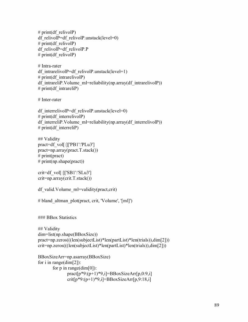
89

# print(df_relivolP) df_relivolP=df_relivolP.unstack(level=0) # print(df_relivolP) df_relivolP=df_relivolP.P # print(df_relivolP) # Intra-rater df_intrarelivolP=df_relivolP.unstack(level=1) # print(df_intrarelivolP) df_intrareliP.Volume_ml=reliability(np.array(df_intrarelivolP)) # print(df_intrareliP) # Inter-rater df_interrelivolP=df_relivolP.unstack(level=0) # print(df_interrelivolP) df_interreliP.Volume_ml=reliability(np.array(df_interrelivolP)) # print(df_interreliP) ## Validity pract=df_vol[:]['PB1':'PLu3'] pract=np.array(pract.T.stack()) # print(pract) # print(np.shape(pract)) crit=df_vol[:]['SB1':'SLu3'] crit=np.array(crit.T.stack()) df_valid.Volume_ml=validity(pract,crit) # bland_altman_plot(pract, crit, 'Volume', '[ml]') ### BBox Statistics ## Validity dim=list(np.shape(BBoxSize)) pract=np.zeros(((len(subjectList)*len(partList)*len(trials)),dim[2])) crit=np.zeros(((len(subjectList)*len(partList)*len(trials)),dim[2])) BBoxSizeArr=np.asarray(BBoxSize) for i in range(dim[2]): for p in range(dim[0]): pract[p*9:(p+1)*9,i]=BBoxSizeArr[p,0:9,i] crit[p*9:(p+1)*9,i]=BBoxSizeArr[p,9:18,i]

90

df_valid.BoundingBox_x_cm=validity(pract[:,0],crit[:,0]) df_valid.BoundingBox_y_cm=validity(pract[:,1],crit[:,1]) df_valid.BoundingBox_z_cm=validity(pract[:,2],crit[:,2]) ## Reliability # print(BBoxSizeArr) concat_BBoxArr=np.concatenate((BBoxSizeArr[0,:,:],BBoxSizeArr[1,:,:],BBoxSizeArr[2,:,:],BBoxSizeArr[3,:,:]),axis=1) # print(concat_BBoxArr) df_BBox=pd.DataFrame(data=concat_BBoxArr) # print(df_BBox) # Used for a quick fix in excel. # writer = pd.ExcelWriter('BBox.xlsx') # df_BBox.to_excel(writer,'Sheet1') # writer.save() # Import BBox2.xlsx df_reliBBox=pd.read_excel('BBox2.xlsx') ## Reliability X df_reliBBoxx=df_reliBBox[['Lisax','Celix','Mikex','Nickx']] df_reliBBoxx.columns=['Lisa','Celi','Mike','Nick'] df_reliBBoxx=df_reliBBoxx.stack(level=0) df_reliBBoxx=df_reliBBoxx.unstack(level=0) df_reliBBoxxP=df_reliBBoxx.P # Inter-Rater Reliability df_interreliBBoxxP=df_reliBBoxxP.unstack(level=0) df_interreliP.BoundingBox_x_cm=reliability(np.array(df_interreliBBoxxP)) # Intra-Rater Reliability df_intrareliBBoxxP=df_reliBBoxxP.unstack(level=1) df_intrareliP.BoundingBox_x_cm=reliability(np.array(df_intrareliBBoxxP)) ## Reliability Y df_reliBBoxy=df_reliBBox[['Lisay','Celiy','Mikey','Nicky']] df_reliBBoxy.columns=['Lisa','Celi','Mike','Nick'] df_reliBBoxy=df_reliBBoxy.stack(level=0) df_reliBBoxy=df_reliBBoxy.unstack(level=0) df_reliBBoxyP=df_reliBBoxy.P

91

# Inter-Rater Reliability df_interreliBBoxyP=df_reliBBoxyP.unstack(level=0) df_interreliP.BoundingBox_y_cm=reliability(np.array(df_interreliBBoxyP)) # Intra-Rater Reliability df_intrareliBBoxyP=df_reliBBoxyP.unstack(level=1) df_intrareliP.BoundingBox_y_cm=reliability(np.array(df_intrareliBBoxyP)) ## Reliability Z df_reliBBoxz=df_reliBBox[['Lisaz','Celiz','Mikez','Nickz']] df_reliBBoxz.columns=['Lisa','Celi','Mike','Nick'] df_reliBBoxz=df_reliBBoxz.stack(level=0) df_reliBBoxz=df_reliBBoxz.unstack(level=0) df_reliBBoxzP=df_reliBBoxz.P # Inter-Rater Reliability df_interreliBBoxzP=df_reliBBoxzP.unstack(level=0) df_interreliP.BoundingBox_z_cm=reliability(np.array(df_interreliBBoxzP)) # Intra-Rater Reliability df_intrareliBBoxzP=df_reliBBoxzP.unstack(level=1) df_intrareliP.BoundingBox_z_cm=reliability(np.array(df_intrareliBBoxzP)) ### KJC stats ## import data df_KJCvalid, df_KJCreli = importKJCdata() # print(df_KJCvalid) # print(df_KJCreli) ## Reliability X df_reliKJCx=df_KJCreli[['Lisa_x','Celi_x','Mike_x','Nick_x']] # print(df_reliKJCx) df_reliKJCx.columns=['Lisa','Celi','Mike','Nick'] # print(df_reliKJCx) # Intra-Rater Reliability df_intrareliKJCx=df_reliKJCx.stack(level=0)

92

# print(df_intrareliKJCx) df_intrareliKJCx=df_intrareliKJCx.unstack(level=0) # print(df_intrareliKJCx) df_intrareliKJCxP=df_intrareliKJCx.P # print(df_intrareliKJCxP) df_intrareliKJCxP=df_intrareliKJCxP.unstack(level=0) # print(df_intrareliKJCxP) df_intrareliP.KJC_x_cm=reliability(np.array(df_intrareliKJCxP)) # print(df_intrareliP) # Inter-Rater Reliability df_interreliKJCx=df_reliKJCx.stack(level=0) # print(df_interreliKJCx) df_interreliKJCx=df_interreliKJCx.unstack(level=0) # print(df_interreliKJCx) df_interreliKJCxP=df_interreliKJCx.P # print(df_interreliKJCxP) df_interreliKJCxP=df_interreliKJCxP.unstack(level=1) # print(df_interreliKJCxP) df_interreliP.KJC_x_cm=reliability(np.array(df_interreliKJCxP)) # print(df_interreliP) ## Reliability Y df_reliKJCy=df_KJCreli[['Lisa_y','Celi_y','Mike_y','Nick_y']] df_reliKJCy.columns=['Lisa','Celi','Mike','Nick'] # Intra-Rater Reliability df_intrareliKJCy=df_reliKJCy.stack(level=0) df_intrareliKJCy=df_intrareliKJCy.unstack(level=0) df_intrareliKJCyP=df_intrareliKJCy.P df_intrareliKJCyP=df_intrareliKJCyP.unstack(level=0) df_intrareliP.KJC_y_cm=reliability(np.array(df_intrareliKJCyP)) # Inter-Rater Reliability df_interreliKJCy=df_reliKJCy.stack(level=0) df_interreliKJCy=df_interreliKJCy.unstack(level=0) df_interreliKJCyP=df_interreliKJCy.P df_interreliKJCyP=df_interreliKJCyP.unstack(level=1) df_interreliP.KJC_y_cm=reliability(np.array(df_interreliKJCyP)) ## Reliability Z

93

df_reliKJCz=df_KJCreli[['Lisa_z','Celi_z','Mike_z','Nick_z']] df_reliKJCz.columns=['Lisa','Celi','Mike','Nick'] # Intra-Rater Reliability df_intrareliKJCz=df_reliKJCz.stack(level=0) df_intrareliKJCz=df_intrareliKJCz.unstack(level=0) df_intrareliKJCzP=df_intrareliKJCz.P df_intrareliKJCzP=df_intrareliKJCzP.unstack(level=0) df_intrareliP.KJC_z_cm=reliability(np.array(df_intrareliKJCzP)) # Inter-Rater Reliability df_interreliKJCz=df_reliKJCz.stack(level=0) df_interreliKJCz=df_interreliKJCz.unstack(level=0) df_interreliKJCzP=df_interreliKJCz.P df_interreliKJCzP=df_interreliKJCzP.unstack(level=1) df_interreliP.KJC_z_cm=reliability(np.array(df_interreliKJCzP)) ## Validity x,y,z df_valid.KJC_x_cm=validity(np.array(df_KJCvalid.xP),np.array(df_KJCvalid.xS)) df_valid.KJC_y_cm=validity(np.array(df_KJCvalid.yP),np.array(df_KJCvalid.yS)) df_valid.KJC_z_cm=validity(np.array(df_KJCvalid.zP),np.array(df_KJCvalid.zS)) print(df_valid) # print(df_interreliP) # print(df_intrareliP) ### CSA concat_CSA=np.concatenate((CrossSurfArea[0,:,:],CrossSurfArea[1,:,:],CrossSurfArea[2,:,:],CrossSurfArea[3,:,:]), axis=1) rowtrial=6*('1','2','3') rowpart=2*(3*('B',)+3*('La',)+3*('Lu',)) rowdev=9*('P',)+9*('S',) rowmultiInd=[np.array(rowdev),np.array(rowpart),np.array(rowtrial)] limbcol=4*(15*('Shank',) + 15*('Thigh',)) subcol=30*('Lisa',) + 30*('Celi',)+30*('Mike',)+30*('Nick',) sectcol=8*('1','2','3','4','5','6','7','8','9','10','11','12','13','14','15') colmultiInd=[np.array(subcol),np.array(limbcol),np.array(sectcol)] df_CSA=pd.DataFrame(data=concat_CSA,index=rowmultiInd,columns=colmultiInd) df_validCSA=df_CSA.stack(level=0)

94

## Shank df_validCSASh=df_validCSA.Shank df_validCSASh=df_validCSASh.stack(level=0) df_validCSASh=df_validCSASh.unstack(level=0) # print(df_validCSASh) df_validCSAShP=df_validCSASh.P df_validCSAShP=df_validCSAShP.unstack(level=3) df_validCSAShS=df_validCSASh.S df_validCSAShS=df_validCSAShS.unstack(level=3) # print(df_validCSAShS[str(1)]) ## Thigh df_validCSATh=df_validCSA.Thigh df_validCSATh=df_validCSATh.stack(level=0) df_validCSATh=df_validCSATh.unstack(level=0) df_validCSAThP=df_validCSATh.P df_validCSAThP=df_validCSAThP.unstack(level=3) df_validCSAThS=df_validCSATh.S df_validCSAThS=df_validCSAThS.unstack(level=3) # print(df_validCSAThS[str(1)]) ## Validity Stats bias_CSASh=np.zeros((15,6)) bias_CSATh=np.zeros((15,6)) for i in range(1,16): practSh=np.array(df_validCSAShP[str(i)]) critSh=np.array(df_validCSAShS[str(i)]) statsSh=validity(practSh,critSh) practTh=np.array(df_validCSAThP[str(i)]) critTh=np.array(df_validCSAThS[str(i)]) statsTh=validity(practTh,critTh) for j in range(6): bias_CSASh[i-1,j]=statsSh[j] bias_CSATh[i-1,j]=statsTh[j] ## Create dataframe from stats rows=np.array(range(0,100,7)) cols=np.array(['mbias','mbiasLCL','mbiasUCL','relmbias','relmbiasLCL','relmbiasUCL'])

95

df_biasCSASh=pd.DataFrame(data=bias_CSASh,index=rows, columns=cols) df_biasCSATh=pd.DataFrame(data=bias_CSATh,index=rows, columns=cols) # print(df_biasCSASh) # print(df_biasCSATh) # Bland-Altman Plot data1=np.array(df_validCSASh.P) data2=np.array(df_validCSASh.S) bland_altman_plot(data1, data2, 'Shank CSA', '[cm2]') data1=np.array(df_validCSATh.P) data2=np.array(df_validCSATh.S) bland_altman_plot(data1, data2, 'Thigh CSA', '[cm2]') ### df_valid=df_valid.T df_interreliP=df_interreliP.T df_intrareliP=df_intrareliP.T writer = pd.ExcelWriter('StatsTable.xlsx') df_valid.to_excel(writer,'Validity') df_interreliP.to_excel(writer,'Intra-Rater Reliability') df_intrareliP.to_excel(writer,'Inter-Rater Reliability') writer.save() end = time.time() print(end - start)

6.1.2 importKJCdata.py import pandas as pd import numpy as np def importKJCdata(): folder='/Users/Olivier/3DAnalysisSession1/' filename='KJC data - PandaImport.xlsx' filepath=folder+filename df_out=pd.read_excel(filepath) filename='KJC data - PandaImport2.xlsx' filepath=folder+filename df_KJCreli=pd.read_excel(filepath) df_out.set_index('Trial', inplace=True)

96

# Get x values df_KJCx=df_out[['Lisa_x','Celi_x','Mike_x','Nick_x']] # print(df_KJCx) # df_KJCxP=pd.concat([df_KJCx.Lisa_x['BP1':'LuP3'],df_KJCx.Celi_x['BP1':'LuP3'],df_KJCx.Mike_x['BP1':'LuP3'],df_KJCx.Nick_x['BP1':'LuP3']] df_KJCxS=df_KJCx.Lisa_x['BS1':'LuS3'] df_KJCxS=df_KJCxS.append(df_KJCx.Celi_x['BS1':'LuS3']) df_KJCxS=df_KJCxS.append(df_KJCx.Mike_x['BS1':'LuS3']) df_KJCxS=df_KJCxS.append(df_KJCx.Nick_x['BS1':'LuS3']) df_KJCxP=df_KJCx.Lisa_x['BP1':'LuP3'] df_KJCxP=df_KJCxP.append(df_KJCx.Celi_x['BP1':'LuP3']) df_KJCxP=df_KJCxP.append(df_KJCx.Mike_x['BP1':'LuP3']) df_KJCxP=df_KJCxP.append(df_KJCx.Nick_x['BP1':'LuP3']) # print(df_KJCxP) # print(df_KJCxS) # df_KJCxS=pd.concat([df_KJCx.Lisa_x['BS1':'LuS3'],df_KJCx.Celi_x['BS1':'LuS3'],df_KJCx.Mike_x['BS1':'LuS3'],df_KJCx.Nick_x['BS1':'LuS3']]) # Get y values df_KJCy=df_out[['Lisa_y','Celi_y','Mike_y','Nick_y']] df_KJCyS=df_KJCy.Lisa_y['BS1':'LuS3'] df_KJCyS=df_KJCyS.append(df_KJCy.Celi_y['BS1':'LuS3']) df_KJCyS=df_KJCyS.append(df_KJCy.Mike_y['BS1':'LuS3']) df_KJCyS=df_KJCyS.append(df_KJCy.Nick_y['BS1':'LuS3']) df_KJCyP=df_KJCy.Lisa_y['BP1':'LuP3'] df_KJCyP=df_KJCyP.append(df_KJCy.Celi_y['BP1':'LuP3']) df_KJCyP=df_KJCyP.append(df_KJCy.Mike_y['BP1':'LuP3']) df_KJCyP=df_KJCyP.append(df_KJCy.Nick_y['BP1':'LuP3']) # Get x values df_KJCz=df_out[['Lisa_z','Celi_z','Mike_z','Nick_z']] df_KJCzS=df_KJCz.Lisa_z['BS1':'LuS3']

97

df_KJCzS=df_KJCzS.append(df_KJCz.Celi_z['BS1':'LuS3']) df_KJCzS=df_KJCzS.append(df_KJCz.Mike_z['BS1':'LuS3']) df_KJCzS=df_KJCzS.append(df_KJCz.Nick_z['BS1':'LuS3']) df_KJCzP=df_KJCz.Lisa_z['BP1':'LuP3'] df_KJCzP=df_KJCzP.append(df_KJCz.Celi_z['BP1':'LuP3']) df_KJCzP=df_KJCzP.append(df_KJCz.Mike_z['BP1':'LuP3']) df_KJCzP=df_KJCzP.append(df_KJCz.Nick_z['BP1':'LuP3']) # write to a DataFrame for all validity values dict_valid={'xP':np.array(df_KJCxP),'xS':np.array(df_KJCxS),'yP':np.array(df_KJCyP),'yS':np.array(df_KJCyS),'zP':np.array(df_KJCzP),'zS':np.array(df_KJCzS)} # df_valid=pd.concat([df_KJCxP,df_KJCxS],axis=1,ignore_index=True) df_valid=pd.DataFrame(dict_valid) # print(df_valid) # print(df_valid.xP) # print(df_valid.xS) return df_valid, df_KJCreli

6.2 Smartphone camera scanning procedure step-by-step 1. Stand in an area with even lighting and no shade (diffused lighting).

a. Find a location on the ceiling that is symmetrically located between lights.

2. The participant should stand with one leg forward, in a semi-lunge position, with the

foot on a white piece of A4 paper. The leg that will be scanned is the forward leg.

3. Flex the forward leg to have a 90º ankle angle and approximately 50-degree knee

angle. The shank should be perpendicular to the ground.

4. The participant should remain completely still until scanning is complete. If any

movement from the participant or in the background occurs, the scan may not be

successful.

5. The scanner should start in a crouched position aiming the phone’s camera on the left

of the knee joint (medial for the right limb and lateral for the left limb). The camera

should be set to capture in portrait view. This allows capturing the whole leg in the

picture including the A4 paper. The leg should be taking as much space as possible in

the camera view.

98

6. Start recording and wait 3 seconds. This will capture the left view of the leg.

7. Slowly stand up keeping the whole leg in the video and wait 1 second

8. Walk slowly around the leg until you reach the front view. Wait 1 second.

9. Crouch down to capture a perpendicular view of the front leg. Wait 3 seconds while

capturing this front view.

10. Still in the same recording, repeat steps 7-10 for the right view, back view and a second

left view.

11. The video recording should be 1-1.5 minutes in length. If the video is less than 1

minute the mesh reconstruction may fail due to insufficient and blurred video frames.

Blurry frames occur when the motion is too fast/jerky. It is better to take a longer video

with better image quality than a faster video with too much motion blur.

6.3 Mesh Processing step-by-step 1) Import 360 video into a “video to JPG converter” software and extract 100 images

2) Open Autodesk Recap and click “create new model”

3) Click “add photos” and open all images obtained in step 1

4) Click “create model”. Keep all settings to default values

5) The images will be uploaded to the Autodesk Recap servers where the 3D

reconstruction will occur. An email notification will be sent to the account email once

the reconstruction is complete and ready to be downloaded

6) Once the reconstruction is complete click on the download button of the new file at

the bottom of the Autodesk Recap window

7) Open the downloaded file to see the full 3D mesh generated.

8) Visually inspect the model with the drag, zoom and rotate tools to ensure no significant

deformations are present (i.e:

9) Use the orbit and zoom view tools to visually inspect for mesh imperfections i.e: holes,

bumps and surface deformations.

10) Crop the mesh to the geometry of interest: the A4 paper, the foot and as much of the

test leg as possible.

a. This can be done with five plane cuts: one plane cut for each side of the A4

paper and one plane cut at the top of the thigh.

99

b. The exact location of the thigh’s plane cut is visually perpendicular to the thigh

axis and immediately distal to where the femur inserts on the pelvis.

11) Scale the mesh with the A4 paper as reference.

a. Measure the longest side of the A4 paper was and then apply the appropriate

scaling factor using the scaling tool.

b. After scaling, measure both sides of the A4 paper to verify that the scale is now

correct (Figure 6).

12) Once the mesh is properly scaled export it as an OBJ (quads) mesh and append

“mesh1” to the file name.

13) Working on the same Autodesk file crop the mesh once more with a plane cut parallel

to the ground and located above the medial malleoli at the smallest circumference of

the shank. This removes the foot and A4 paper from the mesh.

14) Export this new mesh as an OBJ (quads) and append “mesh2” to the name

15) Import “mesh2” into the software Blender and create a duplicate for the following

steps.

a. To reduce noise apply a laplacian smoothing modifier with the following

parameters (Repeat=20, Factor=1, Border=1). The resulting mesh should have

a smooth surface (Factor=1) and borders that curve inwards (Border=1). If this

step mesh is not done prior to designing, then computational issues occur in

future operations (i.e.: mesh conversions and the thickening) which cause

software crashes.

16) Export to smoothed mesh as an OBJ file and append “mesh3” to the file name.

17) It is important that mesh1, mesh2 and mesh3 are saved as OBJ files since this file type

can be converted into T-Spline bodies in Fusion 360. Once these three meshes are

saved the Fusion 360 step-by-step guide can be started

6.4 Fusion 360 step-by-step 1) Create A4 paper representing sketch (sketch1)

a. Create top plane sketch.

b. Draw rectangle with A4 paper dimension

c. Exit sketch

2) Import mesh with A4 paper (mesh1)

100

a. Ensure scale is appropriate by comparing with sketch1

3) Align mesh1 so that the A4 is parallel to the top plane and the top plane cuts through

at the shortest circumference above the medial malleolus

4) Import mesh without A4 paper (mesh3)

a. Ensure scale is same as mesh1

b. Align mesh2 with mesh1

5) Convert mesh3 from quads to T-spline (T1)

6) Create leg cast

a. Thicken T-Spline surface T1 to create a T-spline body

i. Settings

1. round

2. 5mm inwards

3. 8mm outwards

4. total = 13mm ~ 0.5in

b. Convert T-spline body to B-rep body (B1)

7) Determine center of rotation

a. Create sagittal sketch

b. Draw 2-lines representing the leg in 2D (sagittal view)

c. 1 line approximates the main axis of the thigh

d. 1 line approximates the main axis of the shank

e. where the 2 lines connect is the approximated center of rotation of the knee

f. position is determined manually/visually

8) Import hinges and align with center of rotation and knee angle

9) Cut out the knee brace cuffs from the leg cast

a. Create side sketch

b. Draw side view template of knee brace

i. From sagittal view, brace side bars end 2-3 inches away orthogonally

from hinges

ii. Round the open corners of the brace

c. Extrude cut knee brace sketch from leg cast

10) Fillet edges of brace cuffs

101

a. 5mm radius

11) Connect hinges to knee brace cuffs

a. Loft faces of side bars to the corresponding hinges connection

12) Extrude cut slots for straps

13) Extrude cut EMG sensor locations

a. Follow SENIAM guide

14) Fillet all remaining sharp edges

15) Export to STL

16) 3D print

a. 4 mm top/bottom thickness

b. 4 mm shell thickness

c. Gradual infill steps

102

7 References

[1] K. G. Shea, R. Pfeiffer, J. H. Wang, M. Curtin, and P. J. Apel, “Anterior Cruciate

Ligament Injury in Pediatric and Adolescent Soccer Players : An Analysis of Insurance

Data,” J. Pediatr. Orthop., vol. 24, no. 6, pp. 623–628, 2004.

[2] “ACL injuries in young female athletes now an epidemic | Orthopaedics | Loyola

Medicine.” [Online]. Available: https://www.loyolamedicine.org/news/acl-injuries-

young-female-athletes-now-epidemic-04302014. [Accessed: 14-May-2017].

[3] Q. A. Louw, J. Manilall, and K. A. Grimmer, “Epidemiology of knee injuries among

adolescents: a systematic review.,” Br. J. Sports Med., vol. 42, no. 1, pp. 2–10, Jan.

2008.

[4] P. A. Harmer, “Basketball injuries.,” Med. Sport Sci., vol. 49, pp. 31–61, 2005.

[5] S. Colby, A. Francisco, B. Yu, D. Kirkendall, M. Finch, and W. Garrett,

“Electromyographic and Kinematic Analysis of Cutting Maneuvers Implications for

Anterior Cruciate Ligament Injury.”

[6] B. E. Oiestad, I. Holm, L. Engebretsen, and M. A. Risberg, “The association between

radiographic knee osteoarthritis and knee symptoms, function and quality of life 10-15

years after anterior cruciate ligament reconstruction.,” Br. J. Sports Med., vol. 45, no.

7, pp. 583–8, Jun. 2011.

[7] H. Roos, T. Adalberth, L. Dahlberg, and L. S. Lohmander, “Osteoarthritis of the knee

after injury to the anterior cruciate ligament or meniscus: the influence of time and

age,” Osteoarthr. Cartil., vol. 3, no. 4, pp. 261–267, Dec. 1995.

[8] L. S. Lohmander, A. Östenberg, M. Englund, and H. Roos, “High prevalence of knee

osteoarthritis, pain, and functional limitations in female soccer players twelve years

after anterior cruciate ligament injury,” Arthritis Rheum., vol. 50, no. 10, pp. 3145–

3152, Oct. 2004.

[9] L. S. Lohmander, P. M. Englund, L. L. Dahl, and E. M. Roos, “The Long-term

Consequence of Anterior Cruciate Ligament and Meniscus Injuries,” Am. J. Sports

Med., vol. 35, no. 10, pp. 1756–1769, Oct. 2007.

[10] M. V. Paterno, L. C. Schmitt, K. R. Ford, M. J. Rauh, G. D. Myer, B. Huang, and T. E.

Hewett, “Biomechanical Measures during Landing and Postural Stability Predict

103

Second Anterior Cruciate Ligament Injury after Anterior Cruciate Ligament

Reconstruction and Return to Sport,” Am. J. Sports Med., vol. 38, no. 10, pp. 1968–

1978, Oct. 2010.

[11] M. Goddard, L. Salmon, A. Waller, E. Papapetros, and L. A. Pinczewski, “Incidence

of graft rupture 15 years after bilateral anterior cruciate ligament reconstructions,” Bone

Joint J., vol. 95–B, no. 6, pp. 798–802, Jun. 2013.

[12] T. Leys, L. Salmon, A. Waller, J. Linklater, and L. Pinczewski, “Clinical Results and

Risk Factors for Reinjury 15 Years After Anterior Cruciate Ligament Reconstruction,”

Am. J. Sports Med., vol. 40, no. 3, pp. 595–605, Mar. 2012.

[13] E. Laboute, L. Savalli, P. Puig, P. Trouve, G. Sabot, G. Monnier, and B. Dubroca,

“Analysis of return to competition and repeat rupture for 298 anterior cruciate ligament

reconstructions with patellar or hamstring tendon autograft in sportspeople,” Ann. Phys.

Rehabil. Med., vol. 53, no. 10, pp. 598–614, Dec. 2010.

[14] H. Grindem, L. Snyder-Mackler, H. Moksnes, L. Engebretsen, and M. A. Risberg,

“Simple decision rules can reduce reinjury risk by 84% after ACL reconstruction: the

Delaware-Oslo ACL cohort study,” Br. J. Sports Med., May 2016.

[15] L. C. Decoster and J. C. Vailas, “Functional anterior cruciate ligament bracing: a survey

of current brace prescription patterns.,” Orthopedics, vol. 26, no. 7, p. 701–6;

discussion 706, 2003.

[16] D. Théoret and M. Lamontagne, “Study on three-dimensional kinematics and

electromyography of ACL deficient knee participants wearing a functional knee brace

during running,” Knee Surgery, Sport. Traumatol. Arthrosc., vol. 14, no. 6, pp. 555–

563, 2006.

[17] M. A. Risberg, “The Effect of Knee Bracing After Anterior Cruciate Ligament

Reconstruction,” Am. J. Sports Med., vol. 27, no. 1, 1999.

[18] E. M. Wojtys, S. U. Kothari, and L. J. Huston, “Anterior cruciate ligament functional

brace use in sports.,” Am. J. Sports Med., 1994.

[19] J. Styf, “The effects of functional knee bracing on muscle function and performance,”

Sport. Med., vol. 28, no. 2, pp. 77–81, 1999.

[20] M. Jalali, F. Farahmand, T. Rezaeian, D. K. Ramsey, and S. M. E. Mousavi,

“Electromyographic analysis of anterior cruciate deficient knees with and without

104

functional bracing during lunge exercise,” Prosthet. Orthot. Int., vol. 40, no. 2, pp. 270–

276, Apr. 2016.

[21] H. Hart, N. Collins, D. Ackland, and K. Crossley, “Individuals with osteoarthritis after

ACL reconstruction experience immediate improvements in knee pain and confidence

with an unloader knee brace,” J. Sci. Med. Sport, vol. 15, p. S355, Dec. 2012.

[22] E. M. Wojtys, S. U. Kothari, and L. J. Huston, “Anterior Cruciate Ligament Functional

Brace Use in Sports*.”

[23] P. J. Mcnair, S. N. Stanley, and G. R. Strauss, “Knee Bracing: Effects on

Proprioception,” 1996.

[24] K. E. Wilk, L. C. Macrina, and C. Arrigo, “Shoulder Rehabilitation,” 2012.

[25] “Custom Knee Brace Cost.” [Online]. Available: https://www.orthomed.ca/store/knee-

braces?type=113&gclid=CjwKCAjw06LZBRBNEiwA2vgMVfhBTyUvjozBBMiKh

QKEE8KePnk6UzbI2A7j0nERB6crROEEhfn2ZhoCOcUQAvD_BwE. [Accessed:

19-Jun-2018].

[26] A. E. Rankin, “A Survey of Functional Knee Brace Usage Following Anterior Cruciate

Ligament Reconstruction -A Pilot Study,” University of Western Ontario, 1997.

[27] How It’s Made Show, “How Its Made Custom Knee Braces,” 2016. [Online].

Available: https://www.youtube.com/watch?v=o-any6WJNPg. [Accessed: 07-Aug-

2018].

[28] D. Mourtzis and M. Doukas, “Decentralized Manufacturing Systems Review:

Challenges and Outlook,” Springer, Berlin, Heidelberg, 2013, pp. 355–369.

[29] P. Garrehy, “Centralized vs Decentralized Manufacturing,” Industry Today, 2014.

[30] J.-C. Andre, A. Le Mehaute, and O. De Witte, “Fr 2567668.” p. 15, 1984.

[31] Total 3D Printing, “How Much Do 3D Printers Cost? - Price Ranges and Categories,”

2017. [Online]. Available: https://total3dprinting.org/much-3d-printers-cost-price-

ranges-categories/. [Accessed: 07-Aug-2018].

[32] Ultimaker, “Ultimaker S5 specifications,” 2018. [Online]. Available:

https://ultimaker.com/en/products/ultimaker-s5/specifications. [Accessed: 20-Jul-

2018].

[33] R. K. Chen, Y.-A. Jin, J. Wensman, and A. Shih, “Additive manufacturing of custom

orthoses and prostheses—A review,” Addit. Manuf., vol. 12, pp. 77–89, 2016.

105

[34] Nia Technologies, “Nia Technologies.” [Online]. Available: https://niatech.org/.

[Accessed: 07-Aug-2018].

[35] “Enabling The Future – A Global Network Of Passionate Volunteers Using 3D Printing

To Give The World A "Helping Hand."” [Online]. Available:

http://enablingthefuture.org/. [Accessed: 16-Jul-2018].

[36] C.-W. Tan, F. Coutts, and C. Bulley, “Measurement of lower limb volume: Agreement

between the vertically oriented perometer and a tape measure method,” Physiotherapy,

vol. 99, pp. 247–251, 2013.

[37] Enabling The Future, “e-NABLE DEVICE SIZING,” 2018. [Online]. Available:

http://enablingthefuture.org/resources-2/e-nable-device-sizing/. [Accessed: 07-Aug-

2018].

[38] Y. Dessery and J. Pallari, “Measurements agreement between low-cost and high-level

handheld 3D scanners to scan the knee for designing a 3D printed knee brace.,” PLoS

One, vol. 13, no. 1, p. e0190585, 2018.

[39] E. Seminati, D. C. Talamas, M. Young, M. Twiste, V. Dhokia, and J. L. J. Bilzon,

“Validity and reliability of a novel 3D scanner for assessment of the shape and volume

of amputees’ residual limb models.”

[40] G. E. Armin and E. Armin Gruen, “Digital Photogrammetric Imaging Past Present

Digital Photogrammetric Imaging-Past, Present and Future.”

[41] O. CTI, “How to measure for a CTi?” [Online]. Available:

https://www.ctikneebraces.co.uk/guide-to-cti/how-to-measure.html. [Accessed: 13-

Sep-2018].

[42] Ossur, “Ossur OA Unloader One,” 2013.

[43] New Options Sports, “Fitting Chart.” [Online]. Available:

http://www.newoptionssports.com/Fitting-Chart.html. [Accessed: 13-Sep-2018].

[44] I. Breg, “Fusion® Knee Brace.” [Online]. Available:

https://www.breg.com/products/knee-bracing/functional-ligament/fusion-knee-brace/.

[Accessed: 13-Sep-2018].

[45] P. S. Walker, J. S. Rovick, and D. D. Robertson, “The effects of knee brace hinge design

and placement on joint mechanics,” J. Biomech., vol. 21, pp. 965–974, 1988.

[46] F. H. Gunston, “Polycentric Knee Arthroplasty,” Bone Jt., vol. 53–B, no. 2, pp. 272–

106

277, 1971.

[47] R. M. Lazaro and K. L. Dec, 25 – Knee Orthoses for Sports-Related Issues, Fifth Edit.

Elsevier Inc., 2019.

[48] L. G. Hallén and O. Lindahl, “The Screw-Home Movement in the Knee-Joint,” Acta

Orthop. Scand., vol. 37, no. 1, pp. 97–106, 2009.

[49] K. Rajendran, “Mechanism of locking at the knee joint.,” J. Anat., vol. 143, pp. 189–

94, Dec. 1985.

[50] R. F. Escamilla, “Knee biomechanics of the dynamic squat exercise,” Med. Sci. Sports

Exerc., vol. 33, no. 1, pp. 127–141, 2001.

[51] B. RR, “Knee Braces,” in The Hughston Clinic Sport Medicine Book, B. CL, F. F, and

H. JM, Eds. Baltimore: Williams & Wilkins, 1995, pp. 551–558.

[52] M. J. Salata, A. E. Gibbs, and J. K. Sekiya, “The effectiveness of prophylactic knee

bracing in american football: a systematic review.,” Sports Health, vol. 2, no. 5, pp.

375–9, Sep. 2010.

[53] E. P. France and L. E. Paulos, “In vitro assessment of prophylactic knee brace

function.,” Clin. Sports Med., vol. 9, no. 4, pp. 823–41, Oct. 1990.

[54] J. C. Vailas and M. Pink, “Biomechanical Effects of Functional Knee Bracing,” Sport.

Med., vol. 15, no. 3, pp. 210–218, Mar. 1993.

[55] T. P. Branch and R. E. Hunter, “Functional analysis of anterior cruciate ligament

braces.,” Clin. Sports Med., vol. 9, no. 4, pp. 771–97, Oct. 1990.

[56] P. W. Cawley, E. Paul France, and L. E. Paulos, “The current state of functional knee

bracing research A review of the literature.”

[57] N. Rishiraj, J. E. Taunton, R. Lloyd-Smith, R. Woollard, W. Regan, and D. B. Clement,

“The Potential Role of Prophylactic/Functional Knee Bracing in Preventing Knee

Ligament Injury,” Sport. Med., vol. 39, no. 11, pp. 937–960, Nov. 2009.

[58] S. H. Liu and R. Mirzayan, “Current review. Functional knee bracing.,” Clin. Orthop.

Relat. Res., no. 317, pp. 273–81, Aug. 1995.

[59] France and Paulos, “Knee Bracing.,” J. Am. Acad. Orthop. Surg., vol. 2, no. 5, pp. 281–

287, Oct. 1994.

[60] S. A. Paluska and D. B. McKeag, “Knee braces: current evidence and clinical

recommendations for their use.,” Am. Fam. Physician, vol. 61, no. 2, pp. 411–8, 423–

107

4, Jan. 2000.

[61] “Knee Braces – Breg, Inc.” [Online]. Available: https://www.breg.com/products/knee-

bracing/. [Accessed: 16-Jul-2018].

[62] “DonJoy Products.” [Online]. Available:

https://www.djoglobal.com/products/brand?f%5B0%5D=im_field_brand%3A10&f%

5B1%5D=im_field_anatomy%3A51. [Accessed: 16-Jul-2018].

[63] E. L. Castillo, J. D. Castillo, and M. S. Castillo, “Knee brace with cammed stop lever,”

US4886054A, 1989.

[64] E. S. Grood, D. L. Butler, D. M. Ledyard, and S. D. Hoffman, “Knee brace,”

US5018514A, 1991.

[65] J. K. Rasmusson, “Knee brace,” US5060640A, 1991.

[66] D. P. Harris, M. E. Berkeley, and W. L. McCune, “Floating pivot hinge and knee

brace,” US5074290A, 1990.

[67] “Products | Osskin.” [Online]. Available: http://www.osskin.com/index.php/products/.

[Accessed: 16-Jul-2018].

[68] M. P. Greene, “Four Bar Linkage Knee Analysis.”

[69] R. Shenoy, P. Pastides, and D. Nathwani, “(iii) Biomechanics of the knee and TKR,”

2013.

[70] Fong S. Yang, “Knee brace,” US20180021160A1, 2016.

[71] Brett Owen Bledsoe, “Orthopedic knee brace with dynamically changing medial and

lateral hinges,” US20120271211A1, 2012.

[72] A. Bosshard and S. Kohl, “Knee brace for supporting a knee joint,” EP2959868B1,

2014.

[73] B. D. Beynnon, M. H. Pope, C. M. Wertheimer, R. J. Johnson, B. C. Fleming, C. E.

Nichols, and J. G. Howe, “The effect of functional knee-braces on strain on the anterior

cruciate ligament in vivo,” J. Bone Jt. Surg., vol. 74A, no. 9, pp. 1298–1312, Oct. 1992.

[74] C. A. Soma, P. W. Cawley, S. Liu, and C. T. Vangsness, “Custom-Fit Versus

Premanufactured Braces,” 2004.

[75] E. M. Wojtys and L. J. Huston, “Custom-fit versus off-the-shelf ACL functional

braces.,” Am. J. Knee Surg., vol. 14, no. 3, pp. 157–62, 2001.

[76] G. M. Berke, J. Fergason, J. R. Milani, J. Hattingh, M. McDowell, V. Nguyen, and G.

108

E. Reiber, “Comparison of satisfaction with current prosthetic care in veterans and

servicemembers from Vietnam and OIF/OEF conflicts with major traumatic limb loss,”

J. Rehabil. Res. Dev., vol. 47, no. 4, pp. 361–372, 2010.

[77] R. Gailey, K. Allen, J. Castles, J. Kucharik, and M. Roeder, “Review of secondary

physical conditions associated with lower-limb amputation and long-term prosthesis

use,” vol. 45, no. 1, 2008.

[78] S. Santos, B. Soares, M. Leite, and J. Jacinto, “Design and development of a customised

knee positioning orthosis using low cost 3D printers,” Virtual Phys. Prototyp., vol. 12,

pp. 322–332, 2017.

[79] S. Steiner, “ שטיינר אור | לרגל סד - גמר פרויקט .” [Online]. Available: http://orsteiner-

splintkafo.blogspot.com/. [Accessed: 29-Jul-2018].

[80] fcubed, “Modular Knee Brace - Thingiverse,” 2016. [Online]. Available:

https://www.thingiverse.com/thing:1509833. [Accessed: 24-Jun-2018].

[81] “3D Printed PEEK Bionic Knee Brace | INTAMSYS.” [Online]. Available:

https://www.intamsys.com/case-study-bioneek/. [Accessed: 09-Jul-2018].

[82] “Osskin | The World’s First 3D Printed Custom Knee Brace.” [Online]. Available:

http://www.osskin.com/. [Accessed: 09-Jul-2018].

[83] J. Saleh and K. Dalgarno, “Cost and benefit analysis of fused deposition modelling

(FDM) technique and selective laser sintering (SLS) for fabrication of customised foot

orthoses,” Proc. 4th Int. Conf. Adv. Res. Virtual Rapid Manuf., …, pp. 705–710, 2009.

[84] J. H. P. Pallari, K. W. Dalgarno, and J. Woodburn, “Mass customization of foot

orthoses for rheumatoid arthritis using selective laser sintering,” IEEE Trans. Biomed.

Eng., vol. 57, no. 7, pp. 1750–1756, Jul. 2010.

[85] A. S. Salles and D. E. Gyi, “Delivering personalised insoles to the high street using

additive manufacturing.”

[86] A. S. Salles and D. E. Gyi, “An evaluation of personalised insoles developed using

additive manufacturing.”

[87] C. E. Dombroski, M. E. R. Balsdon, and A. Froats, “The use of a low cost 3D scanning

and printing tool in the manufacture of custom-made foot orthoses: a preliminary

study,” BMC Res. Notes, 2014.

[88] R. Chen, L. Chen, B. Tai, Y. Wang, A. Shih, and J. Wensman, “Additive manufacturing

109

of personalized ankle-foot orthosis,” Proc. NAMRI/SME, vol. 42, no. April 2017, pp.

381–389, 2014.

[89] M. Alam, I. Ahmed Choudhury, A. Bin Mamat, and S. Hussain, “Computer Aided

Design and Fabrication of a Custom Articulated Ankle Foot Orthosis,” J. Mech. Med.

Biol., vol. 15, no. 4, 2015.

[90] F. Gao, W. Carlton, and S. Kapp, “Effects of joint alignment and type on mechanical

properties of thermoplastic articulated ankle-foot orthosis,” Prosthet. Orthot. Int., vol.

35, no. 2, pp. 181–189, Jun. 2011.

[91] W. E. Rogers, R. H. Crawford, J. J. Beaman, and N. E. Walsh, “Fabrication of

prosthetic sockets by selective laser sintering,” in Solid Freeform Fabrication

Symposium Proceedings, 1991, p. Volume 6, Pages 158-163.

[92] J. C. H. Goh, P. V. S. Lee, and P. Ng, “Structural integrity of polypropylene prosthetic

sockets manufactured using the polymer deposition technique,” Proc. Inst. Mech. Eng.

Part H J. Eng. Med., vol. 216, no. 6, pp. 359–368, Jun. 2002.

[93] B. Rogers, A. Gitter, G. Bosker, M. Faustini, M. Lokhande, and R. Crawford, “Clinical

evaluation of prosthetic sockets manufactured by selective laser sintering,” 2001 Solid

Free. Fabr. Symp. Proc., no. March 2015, pp. 505–512, 2001.

[94] J. Y. H. Fuh, W. Feng, and Y. S. Wong, “Modelling, Analysis and Fabrication of

Below-knee Prosthetic Sockets Using Rapid Prototyping,” in Advanced Manufacturing

Technology for Medical Applications, Chichester, UK: John Wiley & Sons, Ltd, 2006,

pp. 207–226.

[95] F. E. H. Tay, M. A. Manna, and L. X. Liu, “Case study A CASD/CASM method for

prosthetic socket fabrication using the FDM technology.”

[96] N. Herbert, D. Simpson, W. D. Spence, and W. Ion, “A preliminary investigation into

the development of 3-D printing of prosthetic sockets,” J. Rehabil. Res. Dev., vol. 42,

no. 2, p. 141, 2005.

[97] D. Freeman and L. Wontorcik, “Stereolithography and prosthetic test socket

manufacture: a cost/benefit analysis,” J. Prosthetics Orthot., vol. 10, no. 1, pp. 17–20,

1998.

[98] B. Rogers, S. Stephens, A. Gitter, G. Bosker, and R. Crawford, “Double-wall,

transtibial prosthetic socket fabricated using selective laser sintering: a case study,” J.

110

Prosthetics Orthot., vol. 12, no. 3, pp. 97–103, 2000.

[99] M. C. Faustini, R. R. Neptune, R. H. Crawford, W. E. Rogers, and G. Bosker, “An

experimental and theoretical framework for manufacturing prosthetic sockets for

transtibial amputees,” IEEE Trans. Neural Syst. Rehabil. Eng., vol. 14, no. 3, pp. 304–

310, 2006.

[100] M. C. Faustini, R. H. Crawford, R. R. Neptune, W. E. Rogers, and G. Bosker, “Design

and Analysis of Orthogonally Compliant Features for Local Contact Pressure Relief in

Transtibial Prostheses,” J. Biomech. Eng., vol. 127, no. 6, p. 946, Nov. 2005.

[101] D. M. Sengeh and H. Herr, “A Variable-Impedance Prosthetic Socket for a Transtibial

Amputee Designed from Magnetic Resonance Imaging Data.”

[102] E. L. Doubrovski, E. Y. Tsai, D. Dikovsky, J. M. P. Geraedts, H. Herr, and N. Oxman,

“Voxel-based fabrication through material property mapping: A design method for

bitmap printing,” Comput. Des., vol. 60, pp. 3–13, 2015.

[103] A. M. Paterson, R. Bibb, R. I. Campbell, and G. Bingham, “Comparing additive

manufacturing technologies for customised wrist splints,” Rapid Prototyp. J., vol. 21,

no. 3, 2015.

[104] J. Evill and O. Evill, “CORTEX - EVILL,” 2013. [Online]. Available:

http://www.evilldesign.com/cortex. [Accessed: 20-Jul-2018].

[105] “ActivArmor | Custom 3D-Printed Casts and Splints.” [Online]. Available:

https://activarmor.com/. [Accessed: 20-Jul-2018].

[106] K. Subburaj, C. Nair, S. Rajesh, S. M. Meshram, and B. Ravi, “Rapid development of

auricular prosthesis using CAD and rapid prototyping technologies Background

information,” J. Oral Maxillofac. Surg, vol. 36, pp. 938–943, 2007.

[107] P. Liacouras, J. Garnes, N. Roman, P. Anton, and G. Gerald T., “Designing and

manufacturing an auricular prosthesis using computed tomography, 3-dimensional

photographic imaging, and additive manufacturing: A clinical report,” J. Prosthet.

Dent., vol. 105, pp. 78–82, 2011.

[108] S. A. Dalley, T. E. Wiste, T. J. Withrow, and M. Goldfarb, “Design of a Multifunctional

Anthropomorphic Prosthetic Hand With Extrinsic Actuation,” 2009.

[109] H. Atakan, “A Multigrasp Hand Prosthesis for Transradial Amputees,” 2010.

[110] J. Zuniga, D. Katsavelis, J. Peck, J. Stollberg, M. Petrykowski, A. Carson, and C.

111

Fernandez, “Cyborg beast: a low-cost 3d-printed prosthetic hand for children with

upper-limb differences,” BMC Res. Notes, vol. 8, no. 1, p. 10, Jan. 2015.

[111] B. J. South, N. P. Fey, G. Bosker, and R. R. Neptune, “Manufacture of Energy Storage

and Return Prosthetic Feet Using Selective Laser Sintering,” J. Biomech. Eng., vol.

132, no. 1, p. 015001, 2010.

[112] J. D. Ventura, G. K. Klute, and R. R. Neptune, “The effects of prosthetic ankle

dorsiflexion and energy return on below-knee amputee leg loading,” JCLB, vol. 26, pp.

298–303, 2011.

[113] “Infill | Professional 3D printing made accessible | Ultimaker.” [Online]. Available:

https://ultimaker.com/en/resources/20416-infill. [Accessed: 14-Jul-2018].

[114] Ultimaker, “Ultimaker 3: Unrivaled print quality.” [Online]. Available:

https://ultimaker.com/en/products/ultimaker-3. [Accessed: 20-Jul-2018].

[115] P. Cain, “Selecting the optimal shell and infill parameters for FDM 3D Printing | 3D

Hubs.” [Online]. Available: https://www.3dhubs.com/knowledge-base/selecting-

optimal-shell-and-infill-parameters-fdm-3d-printing. [Accessed: 14-Jul-2018].

[116] A. B. Varotsis, “Introduction to SLA 3D Printing | 3D Hubs.” [Online]. Available:

https://www.3dhubs.com/knowledge-base/introduction-sla-3d-printing. [Accessed:

20-Jul-2018].

[117] A. B. Varotsis, “Introduction to Metal 3D printing | 3D Hubs.” [Online]. Available:

https://www.3dhubs.com/knowledge-base/introduction-metal-3d-printing. [Accessed:

20-Jul-2018].

[118] GE Additive, “What is Additive Manufacturing? | GE Additive.” [Online]. Available:

https://www.ge.com/additive/additive-manufacturing. [Accessed: 20-Jul-2018].

[119] Wikipedians, “3D Printing,” Wikipedia. .

[120] C. Smyth, “Infill and Strength: Functional Design Doesn’t Stop at the CAD Desk | 3D

Printing for Beginners.” [Online]. Available: http://3dprintingforbeginners.com/infill-

strength/. [Accessed: 13-Jul-2018].

[121] R. G. Budynas and J. K. Nisbett, Shigley’s Mechanical Engineering Design, 9th ed.

New York, NY: McGraw-Hill, 2011.

[122] Innofil3D, “Technical Data Sheet. ABS by Innofil3D BV.” Innofil3D, 2016.

[123] S. Hermann, “(9) INFILL pattern and SHELLS - How to get the maximum

112

STRENGTH out of your 3D prints? - YouTube.” [Online]. Available:

https://www.youtube.com/watch?v=AmEaNAwFSfI. [Accessed: 14-Jul-2018].

[124] K. Álvarez, R. F. Lagos, and M. Aizpun, “Investigating the influence of infill

percentage on the mechanical properties of fused deposition modelled ABS parts,” Ing.

e Investig., vol. 36, no. 3, p. 110, Dec. 2016.

[125] M. Fernandez-Vicente, W. Calle, S. Ferrandiz, and A. Conejero, “Effect of Infill

Parameters on Tensile Mechanical Behavior in Desktop 3D Printing,” 3D Print. Addit.

Manuf., vol. 3, no. 3, pp. 183–192, Sep. 2016.

[126] M. Zens, M. J. Feucht, J. Ruhhammer, A. Bernstein, H. O. Mayr, N. P. Südkamp, P.

Woias, and P. Niemeyer, “Mechanical tensile properties of the anterolateral ligament.,”

J. Exp. Orthop., vol. 2, no. 1, p. 7, Dec. 2015.

[127] T. Spahiu and E. Piperi, “Extracting body dimensions from 3D body scanning,” in 6th

International Conference of Textile, 2014, no. November.

[128] L. Jaeschke, A. Steinbrecher, and T. Pischon, “Measurement of Waist and Hip

Circumference with a Body Surface Scanner: Feasibility, Validity, Reliability, and

Correlations with Markers of the Metabolic Syndrome,” PLoS One, vol. 10, no. 3, p.

e0119430, Mar. 2015.

[129] R. E. Sims, R. Marshall, D. E. Gyi, S. J. Summerskill, and K. Case, “Collection of

anthropometry from older and physically impaired persons: Traditional methods versus

TC2 3-D body scanner,” Int. J. Ind. Ergon., vol. 42, no. 1, pp. 65–72, Jan. 2012.

[130] Z. Taha, MohdAzriAris, Zulkifli Ahmad, MohdHasnunArif Hassan, and Nina Nadia

Sahim, “A Low Cost 3D Foot Scanner for Custom-Made Sport,” Appl. Mech. Mater.,

vol. 440, pp. 369–372, 2014.

[131] J. Rosicky, A. Grygar, P. Chapcak, T. Bouma, and J. Rosicky, “Application of 3D

Scanning in Prosthetic & Orthotic Clinical Practice.”

[132] S. Yamamoto, H. Miyachi, H. Fujii, S. Ochiai, S. Watanabe, and K. Shimozato,

“Intuitive Facial Imaging Method for Evaluation of Postoperative Swelling: A

Combination of 3-Dimensional Computed Tomography and Laser Surface Scanning in

Orthognathic Surgery,” J. Oral Maxillofac. Surg., vol. 74, p. 2506.e1-2506.e10, 2016.

[133] C. E. Coltman, D. E. Mcghee, and J. R. Steele, “Three-dimensional scanning in women

with large, ptotic breasts: implications for bra cup sizing and design,” Ergonomics, vol.

113

60, no. 3, pp. 439–445, 2016.

[134] A. Modabber, F. Peters, K. Kniha, E. Goloborodko, A. Ghassemi, B. Lethaus, F. H. €

Olzle, S. Christian, and M. € Ohlhenrich, “Evaluation of the accuracy of a mobile and

a stationary system for three-dimensional facial scanning,” J. Cranio-Maxillofacial

Surg., vol. 44, pp. 1719–1724, 2016.

[135] K. Khoshelham and S. O. Elberink, “Accuracy and Resolution of Kinect Depth Data

for Indoor Mapping Applications,” Sensors, vol. 12, no. 2, pp. 1437–1454, Feb. 2012.

[136] A. Tursi, G. Kurillo, and R. Bajcsy, “Automatic Detection of Body Landmarks in

Human Body Scans Lower Limb Analysis for Biomedical and Footwear Applications.”

[137] H. Oh and J. Kim, “Patella Shape Extraction from 3D Point Cloud Data for

Personalized Knee Brace,” Springer, Cham, 2017, pp. 160–168.

[138] T. Stoyanov, R. Mojtahedzadeh, H. Andreasson, and A. J. Lilienthal, “Comparative

evaluation of range sensor accuracy for indoor mobile robotics and automated logistics

applications,” Rob. Auton. Syst., 2012.

[139] K. D. Mankoff and T. A. Russo, “The Kinect: a low-cost, high-resolution, short-range

3D camera,” Earth Surf. Process. Landforms, vol. 38, no. 9, pp. 926–936, Jul. 2013.

[140] J. Han, L. Shao, D. Xu, and J. Shotton, “Enhanced computer vision with Microsoft

Kinect sensor: A review,” IEEE Trans. Cybern., vol. 43, no. 5, pp. 1318–1334, 2013.

[141] G. Percoco, “Digital Close Range Photogrammetry for 3D Body Scanning for Custom-

Made Garments.”

[142] “Scanlab Photogrammetry.” [Online]. Available: https://scanlab.ca/. [Accessed: 18-

Jun-2018].

[143] N. Summers, “The real-time motion capture behind ‘Hellblade,’” 2017. [Online].

Available: https://www.engadget.com/2017/08/08/ninja-theory-hellblade-motion-

capture-demo-video/. [Accessed: 18-Jun-2018].

[144] “How we used Photogrammetry to Capture Every Last Detail for Star WarsTM

BattlefrontTM - Star Wars - Official EA Site,” 2015. [Online]. Available:

http://starwars.ea.com/starwars/battlefront/news/how-we-used-photogrammetry.

[Accessed: 18-Jun-2018].

[145] C. Goulding, “3D Printed Props Revolutionize the Film Industry Landscape |

3DPrint.com | The Voice of 3D Printing / Additive Manufacturing.” [Online].

114

Available: https://3dprint.com/185871/3d-printed-props/. [Accessed: 20-Jul-2018].

[146] “Legacy Effects.” [Online]. Available: http://www.legacyefx.com/. [Accessed: 20-Jul-

2018].

[147] Weta Workshop, “Weta Workshop - conceptual design and physical manufacturing for

creative industries » Weta Workshop.” [Online]. Available:

https://www.wetaworkshop.com/. [Accessed: 20-Jul-2018].

[148] N. Lievendag, “SCANN3D Android Photogrammetry App Review - 3D Scan Expert,”

2018. [Online]. Available: https://3dscanexpert.com/scann3d-android-

photogrammetry-app-review/. [Accessed: 18-Jun-2018].

[149] Mathworks, “Uncalibrated Stereo Image Rectification - MATLAB & Simulink,”

2018. [Online]. Available:

https://www.mathworks.com/help/vision/examples/uncalibrated-stereo-image-

rectification.html. [Accessed: 18-Jun-2018].

[150] A. Hernandez and E. Lemaire, “A smartphone photogrammetry method for digitizing

prosthetic socket interiors,” Prosthet. Orthot. Int., vol. 41, no. 2, pp. 210–214, 2017.

[151] Li, Guangkun, Gao, Fan, Wang, and Zhigang, “A Photogrammetry-Based System for

3D Surface Reconstruction of Prosthetics and Orthotics,” 2011.

[152] C. Octavian and R. Mariana, “Photogrammetric Scanning and Applications in

Medicine.”

[153] C. L. Heike, K. Upson, E. Stuhaug, and S. M. Weinberg, “3D digital

stereophotogrammetry: a practical guide to facial image acquisition.”

[154] V. A. Knyaz and S. Yu Zheltov, “Photogrammetric Techniques for Dentisry Analysis,

Planning and Visualisation.”

[155] Z. Majid, A. K. Chong, A. Ahmad, H. Setan, and A. R. Samsudin, “Photogrammetry

and 3D Laser Scanning as Spatial Data Capture Techniques for a National Craniofacial

Database,” Photogramm. Rec., vol. 20, no. 109, pp. 48–68, 2005.

[156] N. Lievendag, “Free 3D Scanning from Video by using just a Smartphone - 3D Scan

Expert,” 2017. [Online]. Available: https://3dscanexpert.com/free-3d-scanning-video-

smartphone/. [Accessed: 19-Jun-2018].

[157] L. G. Farkas, W. Bryson, and J. Klotz, “Is photogrammetry of the face reliable?,”

Plastic and Reconstructive Surgery, vol. 66, no. 3. pp. 346–355, 1980.

115

[158] D. V. Kratky, “Digital Modeling of Limbs in Orthopaedics,” Photogramm. Eng.

Remote Sensing, vol. 41, no. 6, pp. 741–752, 1974.

[159] R. Tokarczyk and S. Mikrut, “Close Range Photogrammetry System For Medicine and

Railways,” Int. Arch. Photogramm. Remote Sens. Spat. Inf. Sci. - ISPRS Arch., vol. 33,

no. B5, pp. 519–524, 2000.

[160] G. Baroni, G. Ferrigno, R. Orecchia, and A. Pedotti, “Real-time three-dimensional

motion analysis for patient positioning veri®cation,” Radiother. Oncol., vol. 54, no. 1,

pp. 21–27, 2000.

[161] J. Fels and S. Fingerhuth, “Anthropometric Data Acquisition using Photogrammetric

Techniques to obtain Acoustic Head-Related Transfer Functions of Children,” in

Proceedings of the CTU Conference, 2004.

[162] B. Blizard, “The Art of Photogrammetry: How To Take Your Photos,” Tested, 2014.

[Online]. Available: https://www.tested.com/art/makers/460142-art-photogrammetry-

how-take-your-photos/. [Accessed: 13-Sep-2018].

[163] Sketchfab Team, “How to set up a successful photogrammetry project,” Sketchfab

Blog, 2015. [Online]. Available: https://blog.sketchfab.com/how-to-set-up-a-

successful-photogrammetry-project/. [Accessed: 13-Sep-2018].

[164] S. Lachambre, S. Lagarde, and C. Jover, “Photogrammetry Workflow,” 2017.

[165] “SENIAM.” [Online]. Available: http://www.seniam.org. [Accessed: 12-May-2017].

[166] E. L. Bukowski, A. Conway, L. A. Glentz, K. Kurland, and M. Lou Galantino, “The

Effect of Iyengar Yoga and Strengthening Exercises for People Living With

Osteoarthritis of The Knee: A Case Series,” Int’l. Q. Community Heal. Educ., vol. 26,

no. 3, pp. 287–305, 2006.

[167] S. L. Kolasinski, M. Garfinkel, A. G. Tsai, W. Matz, A. Van Dyke, and H. R.

Schumacher, “Iyengar Yoga for Treating Symptoms of Osteoarthritis of the Knees: A

Pilot Study,” J. Altern. Complement. Med., vol. 11, no. 4, pp. 689–693, 2005.

[168] Blender, “Laplacian Smooth Modifier — Blender 2.79 Manual.” [Online]. Available:

https://docs.blender.org/manual/en/dev/modeling/modifiers/deform/laplacian_smooth.

html. [Accessed: 08-Feb-2018].

[169] 3D-Fuel, “4KG Engineering Pro PLA / APLA+,” Filaments.ca. [Online]. Available:

https://filaments.ca/products/4kg-engineering-apla-fossil-fuel-black-1-75mm.

116


[170] A. P, “TOP 12 PEEK and ULTEM 3D printers -,” 3Dnatives, 2018. [Online].

Available: https://www.3dnatives.com/en/ranking-3d-printers-peek-ultem020520184/.


[171] 3D-Fuel, “Advanced PLA 3D Printer Filament,” Workday PLA. [Online]. Available:

https://www.3dfuel.com/materials/workday-pla/. [Accessed: 13-Sep-2018].

[172] C. Klahn, D. Singer, and M. Meboldt, “Design Guidelines for Additive Manufactured

Snap-Fit Joints,” Procedia CIRP, vol. 50, pp. 264–269, Jan. 2016.

[173] G. Robertson, G. Caldwell, J. Hamill, G. Kamen, and S. Whittlesey, Research methods

in biomechanics. 2004.

[174] “Spreadsheets for analysis of validity and reliability.” [Online]. Available:

http://sportsci.org/2015/ValidRely.htm. [Accessed: 14-Apr-2018].

[175] W. G. Hopkins, “Measures of Reliability in Sports Medicine and Science.”

[176] J. M. Bland and D. G. Altman, “Measuring agreement in method comparison studies,”

SM181RA Stat. Methods Med. Res., vol. 8, no. 99, pp. 962–2802, 1999.

[177] V. G. de Boer-Wilzing, A. Bolt, J. H. Geertzen, C. H. Emmelot, E. C. Baars, and P. U.

Dijkstra, “Variation in Results of Volume Measurements of Stumps of Lower-Limb

Amputees: A Comparison of 4 Methods,” Arch. Phys. Med. Rehabil., vol. 92, no. 6, pp.

941–946, Jun. 2011.

[178] A. Bolt, V. G. de Boer-Wilzing, J. H. B. Geertzen, C. H. Emmelot, E. C. T. Baars, and

P. U. Dijkstra, “Variation in Measurements of Transtibial Stump Model Volume,” Am.

J. Phys. Med. Rehabil., vol. 89, no. 5, pp. 376–384, May 2010.

[179] T. K. Koo and M. Y. Li, “A Guideline of Selecting and Reporting Intraclass Correlation

Coefficients for Reliability Research,” J. Chiropr. Med., vol. 15, no. 2, pp. 155–163,

2016.

[180] A. Menditto, M. Patriarca, and B. Magnusson, “Understanding the meaning of

accuracy, trueness and precision,” Accredit. Qual. Assur., vol. 12, no. 1, pp. 45–47, Jan.

2007.

[181] “Canada Computers: Samsung S5 5.1" 16MP Refurbished Smartphone -

RedFlagDeals.com.” [Online]. Available: https://www.redflagdeals.com/deal/cell-

phones/samsung-s5-5-1-16-mp-refurbished-smartphone/. [Accessed: 13-Sep-2018].

117

[182] N. Center for Health Statistics, “Anthropometric Reference Data for Children and

Adults: United States, 2011–2014,” 2016.

[183] G. D. Myer, D. Sugimoto, S. Thomas, and T. E. Hewett, “The influence of age on the

effectiveness of neuromuscular training to reduce anterior cruciate ligament injury in

female athletes: a meta-analysis.,” Am. J. Sports Med., vol. 41, no. 1, pp. 203–15, Jan.

2013.

[184] D. A. Santos, J. A. Dawson, C. N. Matias, P. M. Rocha, C. S. Minderico, D. B. Allison,

L. B. Sardinha, and A. M. Silva, “Reference values for body composition and

anthropometric measurements in athletes.,” PLoS One, vol. 9, no. 5, p. e97846, 2014.

A low-cost custom knee brace - uO Research

Documents

Transcript of A low-cost custom knee brace - uO Research