Univers

ity of

Cap

e Tow

n

A LIFE CYCLE ASSESSMENT OF ETHANOL PRODUCED FROM

SUGARCANE MOLASSES

A thesis submitted to the

UNIVERSITY OF CAPE TOWN

In fulfilment of the requirements for the Degree of

MASTER OF SCIENCE IN ENGINEERING

(CHEMICAL ENGINEERING)

By

Edward Theka

B.Sc. (Chemical Engineering), UCT

Department of Chemical Engineering

University of Cape Town

Rondebosch, 7701

CapeTown

SOUTH AFRICA September 2002

Univers

ity of

Cap

e Tow

n

The copyright of this thesis vests in the author. No quotation from it or information derived from it is to be published without full acknowledgement of the source. The thesis is to be used for private study or non-commercial research purposes only.

Published by the University of Cape Town (UCT) in terms of the non-exclusive license granted to UCT by the author.

Synopsis

The environmental performance of production companies is increasingly becoming part of

strategies for the competitive marketing of their products, as consumers grow more aware of

environmental issues surrounding industry. Similar products can be compared by the tool of Life

Cycle Assessment (LCA) from the perspective of their impacts on the environment from which

their production resources are drawn and to which their burdens are released. There is the

inherent perception that products made from renewable resources are environmentally more

desirable than those which are produced from finite resources. This thesis investigates whether

this conception is valid for the case of ethanol produced from biomass, by describing and

interpreting the various stages of the production process by means of an LCA.

Sugarcane (Saccharum o/ficinarum) contains 12 - 17% sugars on a wet basis, and 68 -72% moisture.

The sugar composition is 90% sucrose and 10% glucose or fructose. In the conventional sugar

production industry, syrup containing about 34% sucrose (molasses) remains after sugar crystals

are formed from the clarified juice. This sucrose can be fermented to produce ethanol whose uses

include potable consumption and the production of chemicals, but there is growing interest in its

possible use as an additive for motor-grade gasoline, as well as its use as neat fuel to replace

crude-oil based fuels.

This thesis presents a cradle to gate life cycle study carried out with the aim of determining the

environmental consequences of producing ethanol from sugarcane molasses. The investigation

was done for a sugar producing company in the Kwa-Zulu Natal Province of South Africa,

whose interests also lie in the beneficiation of value addition products from sugarcane.

The goal of the study was to produce a comprehensive inventory of all the energy and material

inputs and outputs involved in the production of the 1 kl (1000 litres) of bio-ethanol, using Life

Cycle Assessment (LCA). Concepts of carbon closure and fossil energy ratio were chosen to represent

measures of the degree of renewability of the system, and the results were compared to values

derived from the literature on life cycle assessments of similar bioenergysystems.

The following stages of the life cycle were investigated:

Agricultural Production (sugarcane growing),

Sugarcane to molasses Process (sugar production process, with molasses as by-product),

Molasses to ethanol Process (fermentation of molasses sugars to ethanol, and distillation),

Road Transportation (of sugarcane, and molasses)

The associated process flows, whose production life-cycles were also covered in the assessment,

included the following processes:

.'

Coal Mining

Electricity Generation

Sulphuric Acid Production

Lime Production

Diesel Production

Fertiliser Production

Primary data from the Agricultural, Sugarcane to molasses and Molasses to ethanol process was

gathered from the production sites of the company; while TEAM'I'M software database

information was used to model the transportation, coal mining, electricity generation, sulphuric

acid lime and diesel production processes. Data published in the literature were used to assess the

relative importance of fertiliser production.

A 26% mass-based allocation of the burdens associated with sugar production was made to the

production of molasses. The results showed that the molasses to ethanol process is the most

fossil energy intensive, requiring 0.74 ton of coal per kl of ethanol produced. This represented

86% of the total fossil energy input into the life cycle. Resultantly, a fossil energy ratio of 1.13 was

calculated, with a corresponding carbon closure of 79% as a result of the fossil carbon dioxide

emissions from the combustion of the coal.

The solar endowment in bagasse was found to be 1.1 times the value of the total fossil primary

energy input, indicating the potential subsidy in fossil energy requirement that the bagasse could

offer.

The sulphate and chloride emissions, and the COD (chemical oxygen demand) in the liquid

effluent of the molasses to ethanol process were found to cause the environmental impact of

highest relative concern, this being the eutrophication of aquatic eco-systems. The second highest

impact of note was the contribution to climate change caused by fossil carbon dioxide, also

originating from this process. Other applicable impact categories on a smaller scale "'ere

photochemical oxidant formation and air acidification.

II

Overall, the process showed no significant sensitivity to the allocation rule used, since the

dominating molasses-to-ethanol sub-process was unaffected by the partition between sugarcane

and molasses.

It was recommended that the integration of the two processes with respect to energy utilisation

and management could significantly improve the fossil energy ratio and carbon closure figures of

the production system, and subsequently minimise the impacts which are of concern from the

current production profile.

Further recommendations on the improvement of the model of the overall process included the

quantification of fugitive hydrocarbon vapour emissions, determination of accurate water usage

figures, and the evaluation of the impact of fertiliser and pesticide usage in the agricultural stages

of the ethanol product life-cycle.

iii

Dedication

This thesis is dedicated to my parents D011Jns andDaphne Theka,fo,' their immeasurable support, commitment

and sacrifices, for the sake of my academic pursuits. Thank you.

iv

Acknowledgements

I would like to thank all the people who helped me with their support, information and advice on

this research.

Special thanks go to my supervisor Dr. Harro von Blottnitz for his excellent guidance on the

project and personal support, and to all the staff from the Company who assisted me with

gathering and compiling the required data.

I would also like to thank my friends Christiaan Ndoro, Zimiti Mudondo and Benjamin

Wanda wanda, for their assistance with editing and proofreading of the thesis.

v

Table of Contents

1. INTRODUCTION ................................................................................................ 1

1.1 Background..... .................... ..... ......................... ..... .. ... ...... .......................... ... ........................ 1

1.2 Problem statetnent ................................................................................................................... 4

1.3 Objectir:es 0/ the researr:h ........................................................................................................... 5

1.4 Statunent o/hypothesis ......................... .................................................................................... 5

1.5 Approach ............................................................................................................................... 6

1.6 Lmitations ............................................................................................................................ 6

1.7 Stnteture if the thesis .............. ................................................................................................. 7

2. LITERA 'flJRE REVIEW .................................................................................... 8

2.1 Usinglife-cyde assessment (L CA) to measure sustainability .......................................................... 8

2.2 Review 0/ bio-energy and bio-etha:nol systems .............................................................................. 11

2.2.1 Background ....................................................................................................... 11

2.2.2 Sources of bioenergy .......................................................................................... 11

2.2.2.1 Residues and wastes ........................................................................................ 11

2.2.2.2 Purpose-grown energy crops ........................................................................... 12

2.2.3 Conversion routes to bio-energy from biomass ................................................... 12

2.2.3.1 Gasification .................................................................................................... 13

2.2.3.2 Anaerobic digestion ........................................................................................ 13

2.2.3.3 Steam turbine combined heat and power .......................................................... 13

2.3 Bio-etha:nol firm bitmass: process routes and techndo'l)I.. ............................................................. 14

2.3.1 Production of bio-ethanol .................................................................................. 14

2.3.1.1 Main liquid bio-fuels ....................................................................................... 14

2.3.1.2 Comparison of bio-diesel and bio-ethanol.. ...................................................... 14

2.3.1.3 Blending ethanol with gasoline ........................................................................ 15

2.3.1.4 Feedstock for ethanol production ....... ~ ............................................................ 16

(a) Maize (grain crops) ............................................................................................. 16

(b) Sugarcane .......................................................................................................... 16

VI

2.3.1.5 Ethanol from molasses .................................................................................... 17

(a) Chemistry of molasses fermentation ................................................................... 17

(b) Alcohol recovery ................................................................................................ 17

2.3.2 The future of biomass processing technology ...................................................... 18

2.4 Describing the environmmrai performance ofbiofuels fom a lifo-cpe perspectiu; ............................. 20

2.4.1 How is the renewability of a bio-fuel assessed? .................................................... 21

2.4.1.1 Carbon balances ............................................................................................. 21

2.4.1.2 Energy balancing: input versus output ............................................................. 22

2.4.2 Other life-cycle based approaches for evaluating biofuel renewability ................... 23

2.4.2.1 Exergy analysis ............................................................................................... 23

2.4.2.2 Emergy analysis .............................................................................................. 23

2.5 Key results fom prr!lJiously studiet:l bio.systeJns ........................................................................... 25

2.5.1 Biomass utilisation from sugarcane processing ..................................................... 25

2.5.1.1 Bio-ethanol production from bagasse as a gasoline additive .............................. 25

2.5.1.2 Electricity generation ...................................................................................... 26

2.5.2 Carbon balances of bioenergy systems ............................................................... 27

2.5.2.1 Carbon closure analysis ................................................................................... 27

2.5.2.2 Avoided emissions from bio-energy systems .................................................... 28

2.5.3 Energy efficiencies of bioenergy systems ............................................................. 30

2.5.4 Concerns raised about bio-fuels .......................................................................... 31

2.5.4.1 Land use ......................................................................................................... 31

2.5.4.2 Gaseous emissions from use of biofuels ........................................................... 32

2.5.4.3 Transportation ................................................................................................ 32

2. 6 OJnclusion oj'rrdeu:uzt literature .......................... ..................................................................... 33

3. GOAL AND SCOPE OF THE LIFE CYCLE ASSESSMENT ............................. 35

3.1 Stawnentoj'hyJx;thesis of study ............................................................................................... 35

3.2 Goal of study ........................................................................................................................ 36

3.3 Scope ................................................................................................................................... 38

3.3.1 System definition and boundary .......................................................................... 38

3.3.2 Impact categories to be studied ........................................................................... 40

3.3.3 Functional unit .................................................................................................. 40

3.3.4 Data quality ....................................................................................................... 41

vii

3.4 c:ondU£ling remarks ............................................................................................................... 41

4. Unit descriptions and inventory preparation ....................................................... .42

(a) Foreground sub-processes ...................................................................................... 43

(b) Background sub-processes ..................................................................................... 44

4.1 AlI.()(I:ltion ............................................................................................................................ 45

4.2 Majar stlh·prrx:esses. ............................................................................................................... 47

4.2.1 Agricultural Processing Data ............................................................................... 47

4.2.2 Sugarcane to Molasses Process: Sugar milling data .............................................. 48

4.2.2.1 Milling & Extraction ....................................................................................... 50

4.2.2.2 Sugar Production ............................................................................................ 50

4.2.2.3 Power Generation ........................................................................................... 51

4.2.2.4 Sugar mill data compilation ............................................................................. 52

4.2.3 Molasses to ethanol Process: Distillery Data ........................................................ 52

4.2.3.1 Process description ......................................................................................... 54

4.2.3.2 Data compilation procedures ........................................................................... 54

4.2.4 Transportation Data ........................................................................................... 55

4.3 A ncillary units and rnaiel compilation ...................................................................................... 56

4.3.1 Interlinking of software modules and process data to produce overall inventory ... 56

4.3.2 Dealing with Fertilizer Production in the life-cycle inventory ................................ 57

4.4 Ou?rall cLtta qttality er.uluation. ............... ................................................................................ 58

4.4.1 Temporal and technological representation ......................................................... 59

4.4.2 Data consistency ................................................................................................ 59

4.5 c:ondusion. ....................................................................... .................................................... 59

5. RESULTS AND INTERPRETATION OF INVENTORY ................................. 60

5.1 IntroductWn .......................................................................................................................... 60

5.2 Material balana!s for the main processes .................................................................................... 60

5.2.1 AgricultUial Operations process data summary .................................................... 60

5.2.2 Sugarcane to molasses Process data summary ...................................................... 61

5.2.3 Molasses to ethanol Process data summary .......................................................... 64

5.3 Discussion of key inputs and outputs ........................................................................................ 66

viii

5.3.1 Resource inputs ................................................................................................. 66

5.3.2 Gaseous emissions ............................................................................................. 67

5.3.3 Water emissions ................................................................................................. 67

5. 4 OrnpariJlgf~ and badeground sub.-proa:ss ............ ......................................................... 68

5. 5 E rnironrnentd performance indicatars for the Molasses to Ethanol Process .................................... 71

5.6 Life cyde performance'l'rlMSun?S based on inu!ntmy data .............................................................. 72

5.6.1 Carbon analyses of the bio-system ...................................................................... 72

5.6.1.1 Process carbon balances .................................................................................. 72

5.6.1.2 Carbon closures for the bio- energy system scenarios ....................................... 73

5.6.2 Fossil energy ratio .............................................................................................. 74

5.7 Analysis of factors 7.i'lJich in/ltterza: the bio-etbmol immtmy ......................................................... 78

5.7.1 Effect of allocation on bio-ethanol inventory ...................................................... 78

5.7 .1.1 Effect of allocation on primary energy requirements ......................................... 79

5.7.1.2 Other notable flows affected by allocation ....................................................... 80

5.7.2 Sensitivity of the bio-ethanol study to the inclusion of other sub-processes ........... 81

5.7.2.1 Influence of the transportation steps ................................................................ 81

5.7.2.2 Effect of including fertiliser production data .................................................... 82

5.7.2.3 Use of toxic chemicals for alcohol production .................................................. 84

5. 8 OJnduding remarks for the irnentory interpretation ... ................................................................. 85

6. LIFE CYCLE IMPACT ASSESSMENT .............................................................. 87

6.1 Int:nxfuction ................................................... ....................................................................... 87

6. 2 Results fom Vnpact catejJJries used to assess i:mentory data .......................................................... 88

6.2.1 Climate Change .................................................................................................. 88

6.2.2 Acidification ...................................................................................................... 89

6.2.3 Nutrient Enrichment .......................................................................................... 92

6.2.4 Photochemical oxidant formation potential.. ....................................................... 92

6.2.5 Ozone depletion ................................................................................................ 96

6.2.6 Human toxicity .................................................................................................. 96

6.2.7 Resource depletion ............................................................................................ 102

6.2.8 Impacts of land use ........................................................................................... 102

6.2.9 Overall contl~butions to impact categories ......................................................... 103

IX

6.2.10 Effect of zero allocation to molasses on impact categories .................................. 106

6.3 Nonnalisat:icn oj'irnpact cate:?fJlY saYreS ............ ....................................................................... 107

6. 4 Summary 0/ the lifo cy::/e bnpact assessment................. ...... .. ... .............................. ................... 110

7. CONCLUSIONS AND RECOMMENDA nONS ............................................. 111

8. REFERENCES ................................................................................................ 116

APPENDICES

APPENDIX A

APPENDIX Bl

APPENDIXB2

APPENDIX C1

APPENDIX C2

Life cycle inventories for the production of bio-ethanol from sugarcane

molasses

Readings summary and re-calculated data for life-cycle calculations from

literature

Life cycle calculations for bio-ethanol production system

Primary data for the sugarcane to molasses process

Primary data for the molasses to ethanol process

x

List of Figures

Figure 2.1 Hierarchy of sustainable production levels .............................................................. 9

Figure 2.2 Biomass to bio-energy routes (Sims, 2001) ............................................................. 12

Figure 2.3 Possible process routes for ethanol production( from Mielenz, 2001) ...................... 18

Figure 2.4 The stages involved in the analysis of a bioenergy system ....................................... 20

Figure 2.5 Carbon closures for different bioenergy systems .................................................... 28

Figure 2.6 Avoided emissions for different bioenergy systems ................................................ 30

Figure 2.7 Fossil energy ratios ............................................................................................... 31

Figure 3.1 System boundary for the life-cycle study ................................................................ 39

Figure 4.1 Foreground and background sub-systems for the LeA. .......................................... 43

Figure 4.2 The sugar-molasses co-production system ............................................................. 45

Figure 4.3 Sugarcane to molasses process .............................................................................. 49

Figure 4.4 Production of molasses and sugar: final stages ....................................................... 51

Figure 4.5 Gate-to-gate profile of molasses-to-ethanol process ............................................... 52

Figure 4.6 Block flow diagram showing major distillery sub-units ........................................... 53

Figure 5.1 Material inputs and outputs for Agricultural operations .......................................... 61

Figure 5.2a Sugarcane to molasses Process data (without partition between products) ............. 62

Figure 5.2b Sugarcane to molasses Process data (with allocation to molasses production) ........ 63

Figure 5.3 Material inputs and outputs for Molasses to ethanol Process .................................. 64

Figure 5.4a A carbon analysis of the combined sugar-ethanol bio-system ................................ 76

Figure 5.4b A carbon analysis of the bio-energy system with allocation to molasses ................. 77

XI

Figure 5.5 Modified system with zero allocation to molasses .................................................. 79

Figure 6.1 IPPC-Greenhouse effect (direct, 20 years) for bio-ethanollife cycle ........................ 90

Figure 6.2 CML-fur Acidification potentials for bio-ethanollife cycle ..................................... 91

Figure 6.3 CML-Eutrophication potentials for bioethanollife cycle ........................................ 94

Figure 6.4 WMO-Photo-oxidant formation potentials for bio-ethanollife-cycle ...................... 95

Figure 6.5 WMO-Ozone depletion potentials for bio-ethanollife cycle ................................... 98

Figure 6.6a USES-Human toxicity potentials for bio-ethanollife cycle .................................... 99

Figure 6.6b CST-Human toxicity potentials for bio-ethanollife-cycle Figure 6.6c CML-Human toxicity potentials for bio-ethanollife cycle ............................................................................ 100

Figure 6.6c CML-Human toxicity potentials for bio-ethanollife cycle .................................... 1 0 1

Figure 6.7 CML-Resource depletion for bioe-thanollife cycleFigure 6.8 Relative contributions of sub-processes to each of he impact categories ........................................................................ 104

Figure 6.8 Relative contributions of sub-processes to each of he impact categories ................. 105

Figure 6.9 Normalised scores for the impact categories studied ............................................. 109

xii

List of Tables

Table 1 Market capacity potential for bio-ethanol .................................................................... 2

Table 2.1 World production of bio-ethanol... ......................................................................... 15

Table 4.1 Agricultural processing data ................................................................................... 48

Table 4.2 Summary of transportation data .............................................................................. 56

Table 4.3 Emissions from ammonia production ..................................................................... 58

Table 5.1 Abridged inventory for bio-ethanol production system ............................................ 65

Table 5.2 Energy values of resource inputs ............................................................................ 66

Table 5.3 Comparing foreground and background sub-processes ............................................ 70

Table 5.4 Eco-indicators (Flows per kilolitre of product alcohol) ............................................ 71

Table 5.5 Energy analysis for unallocated life cycle ................................................................ 79

Table 5.6 Relative intensities of the two transport steps of the study ...................................... 81

Table 5.7 Emissions from ammonia production (adapted for calculation) ............................... 83

Table 6.1 Effect of allocation on impact categories ............................................................... 1 06

Table 6.2 Normalisation factors for impact categories ........................................................... 108

Table 6.3 Normalised scores for the impact categories studied ............................................... 108

xiii

BOD

CML

COD

CST

ETBE

GWP

IPCC

LCA

LCI

MTBE

TEAMTM

USES

VOC

WMO

Glossary of Acronyms

Biological Oxygen Demand

Centre of Environmental Science, Leiden University

Chemical Oxygen Demand

Critical Surface-Time

Ethyl Tertiary Butyl Ether

Global Warming Potential

International Panel on Climate Change

Life Cycle Assessment

Life Cycle Inventory

Methyl Tertiary Butyl Ether

Tools for Environmental Analysis and Management

Uniform System for the Evaluation of Substances

Volatile Organic Compound

World Meteorological Organization

xiv

1. INTRODUCTION

1.1 Background

Effective media communication on the detrimental effects of human activities to our own

environment has resulted in an increased global environmental awareness, and this in turn has

paved the way for a revolution in the thinking and approach taken by industry with regards to

environmental management. Environmental legislation has become more stringent, and the

market response is inclined in favour of products of a less detrimental environmental profile.

Resultantly, environmental differentiation is fast becoming a basis for competitive strategy. A

company can use its environmental profile to gain advantage over its competitors by attracting

new customers and building customer loyalty, and it also allows them to charge a premium price

for their products while erecting barriers for potential new entrants. Environmental reporting by

companies has become a communication tool to convince a broad range of stakeholders,

including consumers, of their commitment to environmental protection. Corporate

environmental reports can range from a simple public relations statement, to a detailed in-depth

examination of policy, practices and future direction (Roy & Vezina, 2001).

Products made in South Africa, and sold into sophisticated European and American markets, face

competition from other producers from these regions, and are hence compelled to meet both the

standards of their competitors, and the demands of their consumers.

Ethanol from biomass is an example of such products; it can be produced from a range of energy

and food crops, and, at least in theory, also from cellulosic and hemi-cellulosic biomass sources.

A variety of markets for the consumption of this product exist, and a general overview is shown

below:

• Transport market - gasoline blending with neat ethanol, gasoline reformulation with

ETBE, bioethanol for new generation cars (fuel cells, hybrid etc), bioethanol fuels for

agricultural machinery)

• Cogeneration market - bioethanol for: abatement (reburning) of NOx in fossil fuel

plants, CO2 trade-off fuel, steam injection turbines, combined-cycle power plants, diesel­

powered generators)

• Domestic market - cooking stoves, lighting, refrigeration, heating and cooling devices

• Chemicals market - ethylene, hydrogen production, glycol ethers, ethyl acrylate, acetic

acids, ethylamines, ethyl acetate, acetaldehyde, ethyl ether.

• Potable alcohol market - ethanol is used in liquors of all sorts, examples being gin,

vodka, tequila, brandy and sherry, amongst others.

Currently, the transport market accounts for 20% of present consumption, while the power and

heat market consumes 10%. The chemicals and domestic markets combined account for the

remaining fraction of the ethanol market.

In the long-term, the breakdown of this global market capacity is projected by Grassi (2000) as

follows:

Table 1 Global market capacity potential for bio-ethanol

I Market Projected capacity (million tpa) I

Transport 550

Power and heat 500

Domestic >100

Chemicals 200 I

It can be seen from these projection figures that the transport market is expected to increase

from the current 20% share to at least 39%, representing an approximately 100% increase in the

transport energy sector and hence shifting the dominance in favour of transport energy (Grassi,

2000).

This shift from predominance for domestic and chemical markets to fuel (energy) markets is

foreseen, based on the possible replacement of MTBE (Methyl Tertiary Butyl Ether) and lead in

gasoline. Ethanol is an octane booster for gasoline, and can be blended with gasoline to replace

conventional additives that have since been identified to cause groundwater contamination and

potential human health problems. In the United States alone, the demand for motor fuel is

around 450 billion litres per annum, and with a 4% shortfall resulting from the removal of

MTBE, an ethanol production of 11 - 15 billion litres would be required, compared to the

current production of 5 billion litres (Lyons, 1999).

In many African countries however, the use oflead in gasoline is still dominant because ofthe

comparative cost of the alternative additives. The investigation by Thomas and Kwong (2001)

2

determined that within the potential of sub-Saharan countries have great potential to produce

ethanol from sugarcane and molasses for blending with ethanol. It was also determined that, for a

20% ethanol blend in gasoline, 2.4 billion litres would be required to replace the 9000 tons lead

per year used in Africa. In the evaluation of the sugarcane industry in these sub-Saharan

countries, up to 0.5 billion litres ethanol per year can be produced from molasses only, and up to

4 billion litres if all sugarcane is converted to ethanol. From these figures, it can be seen that the

potential to meet the required ethanol capacity (2.4 billion litres per yr) for lead replacement in

Africa is collectively feasible.

But do products made from renewable resources, such as ethanol from biomass, necessarily have

an inherent environmental competitive advantage over their counterparts, on the basis of their

natural origin? Market perception is definitely of this opinion, and products that are renewable are

viewed as being of a "greener" profile, and are hence preferred over other products of the same

category. From an overview perspective, this appears a well-justified ideology; biomass is a

renewable resource through the natural carbon cycle of photosynthesis through which it can be

re-generated. But how sustainable is the collective of processes which combine to make these so­

called renewable products? This question can only be comprehensively answered by scrutinising

their full life-cycle and accounting for all the energy and material inputs and outputs involved in

their production, as well as the environmental burdens created in the process and their impacts.

Life-cycle assessment (LCA) offers an approach to analyse and answer the questions above, it is

an effective evaluation tool for the determination of the effects to the environment relating to a

particular product, because of its cradle-to-grave approach, which calls for the inclusion of all

indirect inputs and outputs in the analysis. The results of an LCA are primarily a comprehensive

production inventory, which can then be translated into environmental impacts in different

categories of concern, as well as other performance evaluation indices directed at determining

how intensively damaging a product is to the global environment.

3

1.2 Problem statement

Liquid bio-fuels form an important subset of so-called "bioenergy" systems, which represent one

of the emerging renewable energy options, other examples being solar, wind and hydro-energy.

The exploration of these alternative energy options comes in the wake of the realisation that

current fossil energy consumption is not sustainable. This derives from the observations that,

amongst other environmental concerns, future generations would not be awarded equal privilege

to energy exploitation due to limited availability, and that the current dispersion of combustion

products into the global environment also seems to be resulting in detrimental changes in climate.

Bio-ethanol, used as fuel, is a specific product from the renewable energy source of biomass,

which can be grown purposefully through energy crops or vegetation, but is also naturally

occurring. The inherent question presented in the previous section, which is the essence of the

investigation in this study, is revisited here:

Are the current patterns of production and use of products from replenishable raw

materials sustainable?

The production of bio-ethanol in the African context, where it is mainly a by-process of the sugar

production industry, has (with the exception of several Mauritian studies) not been investigated

from a life-cycle perspective.

As will be discussed in chapter 2, the comparative performance of bio-fuel production systems

has been scrutinised in the context of their energy inputs and outputs, carbon balance profile,

resource use and environmental burdens, amongst other issues of concern with respect to

sustainability. Currently, this level of information detail on ethanol production from molasses has

yet to be attained. The results oflife-cycle approaches to bio-energy systems analyses which have

been previously done show that different aspects of the production profile may be isolated as

being of key concern for the different studies. This makes the particular assessment of the

performance of bio-ethanol production of this nature imperative, before commenting on the

sustainability of the overall process.

Hence, the following problem statement is presented:

There is lacking in the understanding of the extent to which the renewability of bio­

ethanol produced from sugarcane molasses, as produced in Africa, can be stated. Its

processing and use are yet to be determined as sustainable through a comprehensive

4

study of all energy and material inputs and outputs involved in the entire life cycle of the

product, and their conslquences on the receiving environment.

1.3 Objectives of the research

The primary objectives of this life-cycle study are as follows:

• to document a comprehensive life-cycle inventory for the production of ethanol from the

fermentation of molasses from the sugar-processing industry;

• to derive from this inventory an understanding of the implications of the overall process,

in terms of environmental burdens and their subsequent impact on the recipient

environment.

The energy and resource requirements, and the resulting environmental outputs can be

translated into assessment measures and indices which give an indication of the severity

of the overall process in global and regional terms.

Another objective of the study was related to the direct use of the information by the company

involved, and this is to record data at the distillery in such a way that it is of use in the monitoring

of their environmental performance internally, by the use of relevant indicators.

1.4 Statement of hypothesis

Based on the objectives stated above, the hypothesis put forward in this research is then:

Current practices of ethanol production from sugarcane molasses are sustainable in

principle, but may require modifications in the cane growing and processing, and the

conversion process involved. Further, such modifications can be effectively identified

through a life-cycle analysis.

The hypothesis stated here is made with insight into the key questions raised from similar studies,

as uncovered by the literature. It is important to note that the process under scrutiny here has the

prime purpose of producing sugar, and molasses is a by-product stream from which a value­

addition product is produced. The results of this study shall hence be carefully analysed with the

observation that the conversion processes involved are not directly orientated towards the

production of molasses.

5

1.5 Approach

The argument presented in the problem statement (section 1.2) hence sets the platform for the

analysis of this study. In order to prove the hypothesis stated above, the following approach is

proposed:

Initially, the relevance of using life-cycle assessment (LCA) to arrive at the detail of information

required to characterise the sustainability of the current production practices needs to be

affirmed. To this end, literature on sustainability of industrial production is reviewed, and

examples of the applicability of the methodology to this type of problem are sought out.

A more detailed review of previous life cycle based studies on bio-energy systems is then

presented, to highlight the issues of concern which have arisen, and which may be relevant to this

particular investigation. This work also serves to identify the gaps or inadequacies of the

published studies. Finally, this review shall identify the different assessment methods and indices

that have previously been used to describe the renewability of bio-energy systems.

From this platform, a life cycle analysis, with its typical four phases of goal and scope, inventory,

impact assessment, and interpretation is launched of current bio-ethanol production in a South

African setting. The system analysed here is limited to one particular production operation.

Nevertheless, the sugar processing and alcohol production technologies used are largely

conventional in Africa, and hence the analysis is relevant for generalisation~

Finally, the results of this life cycle assessment can be compared with the results from previous

studies, and hence conclusions on the fore-stated hypothesis can be duly made.

The extent of the contribution made by this study is limited by its goals and scope, and the

presentation of these limitations outlines what expectations this analysis should be able to meet.

1.6 Limitations

The main limitation of this LCA is the exclusion of the end-use of the ethanol product. This is

because its current main use is as potable alcohol, while the study seeks to lay a foundation for

the exploration of different possible uses, particularly as biofuel. Resultantly, this is only a cradle­

to-gate life cycle analysis, with the ethanol product as the gate end of the study. By exclusion of

the end-use of this ethanol, the results could be used comparatively with other production life­

cycles to explore the advantages and disadvantages of each where different end-uses are

investigated, such as its use as a substitute fuel or gasoline additive.

6

Another limitation is the fact that this data is specific to the production profile of one company

only, and not averaged to represent general production pattern of this nature. This means that

some results will be specific to the company alone, and may not necessarily reflect the practices of

other similar producers.

Other limitations are in the detail of the data gathered, pertaining to data recording practices at

the production sites, as well as physical constraints, to be further discussed under the relevant

sections.

1.7 Structure of the thesis

The following outline has been used to present the detail of the thesis in the chapters to follow:

• Chapter 2 is the literature review chapter. The subsections discuss, firstly, how life cycle

assessment can be used to measure process sustainability.

The subsequent sections then investigate the different measures of sustainability used in other

studies, and present their results. The sources and technology (present and future) for

producing bio-ethanol are scrutinised, leading to the particular findings of the study in the

next chapter.

• Chapter 3 presents the goal and scope of the LCA.

• Chapter 4 outlines the data gathering procedures used in the study, and also discusses the

modelling of the overall process using the TEAMTM software, which leads to the inventory

results in the subsequent chapter.

• The life-cycle inventory is presented in Chapter 5; the key flows are isolated and discussed,

giving reason for their highlighting, and how this relates to the impact assessment to follow.

An interpretation of the figures in the inventory is made here, and life-cycle based indicators

related to those presented in the literature review are also presented. A sensitivity analysis is

also shown here, examining the effect of allocation and minima and maxima of key flows.

• Chapter 6 presents the impact categories of interest to this study, followed by the actual

figures for impact assessment as generated by the TEAM software. An interpretation of the

impact assessment is presented, and the discussion on this chapter then leads to the

conclusions and recommendations to follow.

• Chapter 7 is the conclusions and recommendations chapter, and draws on the interpretation

of the inventory and the impact assessment, in line with the hypothesis and objectives of the

research.

7

2. LITERATURE REVIEW

This chapter presents the key literature relevant to this study, in line with the objectives and the

approach as described in the previous chapter.

A discussion of how LCA addresses concerns of sustainability is first presented, followed by

details of production of bioenergy from biomass, and bio-ethanol in particular. The life cycle

analyses of bio-energy systems and their results are then presented, and finally the main issues of

concern raised in the production of energy from biomass are highlighted.

2.1 Using life-cycle assessment (LeA) to measure sustainability

LCA has been chosen as the preferred tool for the evaluation presented in this study, and the

section here shall present the features of this tool which make it suitable to evaluate sustainability

of production systems.

The technical definitions of life-cycle assessment (LCA) as J. process evaluation tool, as well as its

operational hierarchy and generic methodology shall not be discussed, as the target audience for

this analysis is deemed to be knowledgeable in the foresaid field. The reader is encouraged to

consult literature references on life-cycle methodology; the guiding documents from which the

adaptation used here was obtained are the ISO standards on life-cycle assessment methodology,

the TEAMTM software (discussed later) manual, and reference to the thesis by Rwodzi (2000).

LCA is a method for assessment of the environmental impact of products, processes or services

from raw materials to waste products. Although this method is often used to compare products

with the same function, it can also be used to identify "hot spots", which are parts ofthe life

cycle which are critical to the overall environmental impact (Anderson et a1.,1998).

It is viewed as an effective tool for sustainable performance, because it holds companies

responsible for considering the upstream and downstream implications of their activities, and

hence take action to mitigate them. The inter-connected industrial system from which a product

is made is carefully considered, paying attention both to the products and by-products, as well as

waste streams, in view of processing and service operations. Consumers are also considered an

integral part of the cycle; they use the products and energy resources, then return them to the

industrial eco-system for reprocessing and re-use (DeSimone & Popoff, 1997).

8

Recent works suggest that there is a five level hierarchy of involvement in the concept of building

sustainable systems of production and consumption. A model developed at the University of

Cape Town, similar to work published elsewhere (Vel eva, 2001), is shown below:

[Level 5] Sustainable systems effects on long-term quality of life & human development; how do we fit into a sustainable society?

[Level 4] ute cycle thinking I management: impacts of product through production, to use, then disposal

[Level 3 ] Continuous improvement: formalise environmental management of operations, open to external audit

[Level 2] Pelformance monitoring & Eco-efficiency: resource use efficiency, can lead to cost savings?

[Levell] Compliance with environmental legislation for effluent, emissions, wastes (minimum requirements); Clean Air Act, Toxic Release Inventory

Figure 2.1 Hierarchy of sustainable production levels

Level one monitoring only evaluates the extent to which a company is in compliance with

regulations, and typically these would be specified by the Occupational Safety and Health Act or

Toxic Release Inventory, for example. Level two reports a facility's inputs and outputs, emissions,

products and waste, and can measure resource use efficiency and can be used for maintaining a

competitive advantage.

Level three is a step further than the previous level, where the company opens itself to external

environmental auditing and begins to take note of the impact of its process on a global scale e.g.

greenhouse gas emissions per year.

Level four monitoring goes beyond the boundary of the firm's processes and extends the level

three reporting to their supply chain, product distribution and ultimate disposal . This is the level

at which life-cycle assessment (LCA) can be used to follow up on the upstream processes that

provide the raw materials, and downstream to the end use of the product.

The study presented here sits at the fourth level. This level is very crucial because it is the first

level at which observation is made beyond the site boundaries of the process, to incorporate the

burdens of upstream production involved with the various flows and utilities associated with the

final product. The information compiled at the fourth level creates an overall picture of the full

implications of it product's manufacture and use, and supplies the background for the analysis

which follows in the fifth level.

Level five essentially involves a multi-disciplinary analysis; it shows how an individual company's

performance fits into a global picture of a sustainable society, looking at the effects of production

on the long-term quality of life and human development. The socio-economic aspects, as well as

the environmental debates surrounding the benefit and/or detriment of a particular product are

assessed at this level.

A level five analysis can only be made comprehensively once the detail from the previous level is

compiled, and therefore the fourth level approach used in this assessment is the appropriate

starting point for a company which aims to establish its contribution to a regional or global

sustainability profile, as is the case here.

10

2.2 Review of bio-energy and bio-ethanol systems

This section and those following shall explore the profiles and performances of different

bioenergy systems, ranging from electricity production to liquid fuels production. While it is

appreciated that the study presented in this research is the production of ethanol for potable use,

the results from a diverse range of bio-energy systems is deemed to be relevant in establishing the

methodological approach and typical results and concerns raised on bio-systems, and this sets a

relevant platform for the analysis of this particular research.

2.2.1 Background

Renewable energy sources make up one-fifth of the world's energy supplies, with 13 - 14%

originating from biomass, and 6% from hydro-power. It is estimated, however, that in developing

countries, biomass can account to up to 90% of all energy used, while in some developed

countries such as Sweden and Finland, its use is in the range of 16 - 18% (Hall & Scrase, 1998). A

study by Churn and Overend (2001) also revealed that in the United States alone, biomass (43%)

is only second to hydropower (51%) as a primary renewable energy source.

Despite its apparent abundance, biomass still remains the least efficiently exploited renewable

energy source, overshadowed by the dominance of hydro-power, solar and wind energy (Sims,

2001). Biomass is most commonly used as fuel, by incinerating it to generate heat. Other routes

of conversion to retrieve biomass energy in other forms are yet to be fully utilised.

Owing to its climate, Africa has an abundance of biomass, and hence the exploration of energy

options which offer its efficient use and maximisation is imperative (Karakezi & Mackenzie,

1993).

2.2.2 Sources of bioenergy

Bioenergy sources can be classified into three main categories:

(i) residues and wastes from agricultural production

(ii) purpose-grown energy crops, and

(iii) natural vegetation.

II

2.2.2.1 Residues and wastes

This refers to trash from agricultural processing such as rice-husks, corncobs, bagasse and cane

tops from sugarcane. Other crops that produce residue which can be used for bio-energy are

barley (straw), coconut (shell), ground nuts (shell), and maize (husks, stalks).

These are an essential source of bio-energy, particularly in regions where most of the land is used

for food production (Kartha & Larson, 2000).

2.2.2.2 Purpose-grown energy crops

These are the crops that are specifically grown for energy conversion, and typical examples are

sugarcane, sugar beet, rapeseed, wheat, maize, sorghum and potatoes (Kaltschmitt et al., 1996). -­

Perrenial grasses, such as switchgrass, big bluestem, reed canary grass and alfalfa have also been

successfully grown for the purpose of energy harvest (Hallam et aI., 2001).

2.2.3 Conversion routes to bio-energy from biomass

Biomass can be converted to bio-energy in the form of heat, power and transport/ macrunery

fuels. The diagram below illustrates the different forms of bio-energy, as well as the processing

routes used for their production:

Anaerobic digestion

methane Heat Animal manures Organic wastes

Green crops l...------;:=~_-.--::--=_-------....~G as 0 lin e

/

Wood residues Woody biom ass crops

Sugar crops Fermentation/

Distillation

Flash

gasification

Pre-hydrolysis + Hydrolysis

(acid /enzym e)

Figure 2.2 Biomass to bio-energy routes (Sims, 2001)

12

Diesel

Methanol

Electricity

E thano I

Brief discussions on some of the technologies illustrated in the figure above (with the exception

of ethanol from sugar crops which is discussed in detail in section 2.2.4) shall follow here to

develop an understanding of the technical diversity in the conversion of the different energy

earners.

2.2.3.1 Gasification

Combustible gas is produced through high-temperature (thermochemical) and low-temperature

(biological) processes. In thermochemical gasification, the biomass is essentially burnt with just

enough air (incomplete combustion) to convert it to gaseous fuel. Updraft and downdraft fixed­

bed gasifiers are used, and the product gas can be used for heating, cooking or for internal

combustion engines to produce electricity or shaft power generation.

2.2.3.2 Anaerobic digestion

In this process, the organic matter is degraded by three kinds of bacteria: fermentative bacteria,

acetogens and methanogens. The fist two break down complex organic compounds into simpler

intermediates, which are then converted to methane and carbon dioxide by methanogens.

2.2.3.3 Steam turbine combined heat and power

Pressurised water is boiled, and the resulting steam is expanded to drive a turbine generator, then

condensed back to water for partial or full recycling to the boiler. A heat exchanger can be used

to recover heat from flue gases and use this to preheat combustion air, and a de-aerator is

required to remove dissolved oxygen from the water before boiling it. The boiler fuel is biomass,

preferably dried to improve the boiler efficiency.

13

2.3 Bio-ethanol from biomass: process routes and technology

2.3.1 Production of bio-ethanol

2.3.1.1 Main liquid bio-fuels

The key liquid bio-fuels that have been researched as potential replacements for fossil fuel are

bio-diesel (from vegetable oil ester), bio-ethanol (from fermentation of sugars in crops) and its

derivative Ethyl Tertiary Butyl Ether (ETBE). Other liquid biofuels such as bio-methanol and its

derivative MTBE (Methyl Tertiary Butyl Ether) from lignocellulosic material have been

researched, but have not gained the commercial potential and market share of the first two

(ATLAS web site, 2001).

2.3.1.2 Comparison of bio-diesel and bio-ethanol

Biodiesel had a worldwide production capacity of 1 263 000 metric tons in 1996, with Germany

and France as the leading producers. In the European Union (EU) alone, production is estimated

at 907 000 metric tons.

The main feedstock for bio-diesel production in Europe is oil from rapeseed, although other

vegetable oils may be used. Its capital use has been in the blending with petroleum diesel for use

in urban-public-bus and truck fleets, but also for fuelling farm equipment, and as a heating fuel,

solvent, hydraulic oil, and lubricant (Raneses et al., 1999). In the United States, bio-diesel is

produced mainly from soybeans.

Until recently, however, Brazil and North America were the only two regions which produced

fuel ethanol from sugarcane and maize, respectively, on a significant commercial scale. Table 2.1

below illustrates the distribution of ethanol production as of 1999, identifying key players in the

industry.

14

Table 2.1 World production of bio-ethanol

Country i Production i Raw materials

l (billion litres) I I Brazil 14.0 • Sugarcane, beets

I United States 5.3 Cereal grains

I i

(mostly corn) I i Europe 4.3 Cereal grains, beets !

i Russia 2.5

• Total world production I 28.0

Berg, 1999, cIted by Lyons, 1999

2.3.1.3 Blending ethanol with gasoline

(a) Background

Cereal grains, beets i

Octane rating is a measure of the tendency of the air and fuel mixture to resist spontaneous

combustion as it is heated during the compression stroke in the engine cylinder of a four-stroke

engine. This pre-ignition, or knock effect, as is commonly known, would otherwise decrease the

efficiency of the engine and increase wear. At high temperatures and pressures during

compression of fuel in the engine, the fuel molecules break down to free radicals, which can then

build up the chain reaction to cause pre-ignition. The role of an additive like tetra-ethyl lead is to

"scavenge" these free radicals, reacting with them before they can cause the said chain reaction.

Changing its composition can, however, increase the octane value of gasoline. By blending with

ethanol, which is a low bond order hydrocarbon, the probability of forming free radicals at high

temperatures and pressures can be reduced (Thomas & Kwong, 2001)

(b) Status and prospects of ethanol as fuel

Brazil's Proalcool Program introduced in 1975, following the energy crisis of the period, set the

pace for the country's leading alcohol programme, which grew from 1 billion litres in 1976 to

12.6 billion htres in 1995 of ethanol from sugarcane. In the Unites States, ethanol is produced

from corn (maize), and is more expensive than the sugarcane based ethanoL As a result, it relies

on a government subsidy of $0.14/1 to make it competitive with gasoline.

In sub-Saharan Africa, South Africa, Zimbabwe, Malawi and Zambia are viewed as having great

potential for fuel ethanol production, based on their current sugar production capacities. Each of

15

these countries is estimated to have a potential cane-to-ethanol production capacity greater than

100 million litres per annum, and a molasses-to-ethanol potential capacity of above 10 million

litres per annum (Thomas & Kwong, 2001)

This forms strong basis for the motivation for the replacement of gasoline additives with ethanol,

but also provides an incentive for the weak economies of these African countries, which could be

boosted by reduced dependency of crude oil imports.

2.3.1.4 Feedstock for ethanol production

There are several feedstock used for ethanol production, as discussed previously. The different

sources shall be discussed here, with attention given to their content and processing techniques.

(a) Maize (grain crops)

Grain crops can be used to produce bio-ethanol by fermentation of the sugars found in them.

Typical grain crops used are maize and wheat.

Processing maize and other grain crops involves wet or dry milling. In wet milling, the grain is

soaked in water with sulphur dioxide for up to 40h, followed by grinding and separation of starch

and co-products. For wheat, the valuable bran and germ are removed first by dry processing in a

flour mill, then soaked in water. The starch fraction is then cooked at low temperatures to

encourage gelatinisation, followed by the addition of a-amylase, which yields dextrin

oligosaccharides.

The final stage of processing is saccharification, where glyco-amylase converts the starch to

glucose, which can then be fermented to alcohol (Wheals et aI., 1999).

(b) Sugarcane

Sugarcane (Saccharum officinarum) contains 12 - 17% sugars on a wet basis, and 68 -72% moisture.

The sugar composition is 90% sucrose and 10% glucose or fructose. Up to 95% efficiency can be

achieved in the extraction of juice from the cane, and the remaining solid residue is cane fibre, or

bagasse.

For an ethanol-only producing process, the cane juice is typically heated to reduce microbial

contamination, then concentrated by evaporation, and then fermented. A sugar-ethanol process,

however, centrifuges the sucrose crystals formed during evaporation, and syrup (molasses)

remains, containing up to 65% w/w sugars.

Both the cane juice and molasses contain sucrose and other sugars which can be fermented to

produce ethanol (Wheals et aI, 1999).

16

2.3.1.5 Ethanol from molasses

Molasses is the feedstock used for the production of the bio-ethanol being studied here, hence

considerable detail of the processing shall be illustrated to establish an understanding of the

process. A more specific description of the particular process for this research will follow in

Chapter 3.

(a) Chemistry of molasses fermentation

The sugars in molasses are mainly in the form of glucose. Sucrose is broken down to glucose via

hydrolysis:

The glucose in turn is fermented to ethanol via the Gay-Lussac equation for ethanol production

from glucose via fermentation:

The process involves dilution of the molasses to 25"Brix required to allow for fermentation to

begin, due to the high osmotic pressure exerted by the sugars and salts. {Brix is the sum of the

dissolved (or dissolvable) matter in a substance expressed as a percentage by mass or as an actual

mass).

Fermentation then takes place at 32 - 3rC, but the maximum temperature may be lowered to

achieve high final alcohol volumes because alcohol inhibition of yeast growth is intensified at

higher temperatures (Mutargh, 1999).

(b) Alcohol recovery

The fermentation product is called beer, and a stripping column is used to separate the dunder

from the liquid alcohol product. The final stage of the alcohol recovery process is distillation. The

ethanol-water mixture, however, forms an azeotrope at 95.4% ethanol purity, and this causes a

high ~nergy requirement for the distillation stage.

17

2.3.2 The future of biomass processing technology

A prediction for future energy scenarios is presented by Shell International Petroleum Company,

cited by Hall and Scrase (1996). In this prediction, biomass becomes a major energy supplier after

2020, supplying up to 14% of energy demands, while solar and wind contribute 17% and 11%

respectively. The biomass percentage contribution is projected to rise even further to 25 - 46%

by the year 2100.

In the light of these visions, extensive research is being carried out to explore efficient methods

of energy retrieval from biomass sources.

An enzyme hydrolysis-based biomass-to-ethanol processing scheme has been proposed, where

the biomass is milled, then treated with steam and dilute sulphuric acid, to open up the ligno­

cellulose pore structure and make it more susceptible to enzyme attack. The ligno-cellulosic solids

are then converted to ethanol in a simultaneous saccharification and fermentation bio-reactor.

The advantage of this technology is that it reduces end-product inhibition of the cellulases by

glucose through continuous fermentative conversion, but it also reduces capital costs by reducing

the number of vessels required to separately carry out hydrolysis and fermentation (i\1cMillan,

1997).

Biomass Conc Acid

Sugar Ethanol

Milling and ~ Acid r- - fermentation f--blending hydrolysis recovery

To ethanol recovery

/ Biomass

Biomass High LOW"TI ,uga. Ethanol Milling and -JIo temp r- Cellulase fermentation r-

blending pretrea tmen t treatmen to ethanol recovery

Enzyme production

Figure 2.3 Possible process routes for ethanol production( from Mielenz, 2001)

18

The diagram above illustrates this route, parallel to an alternative route which requires the pre­

treatment of biomass for both ethanol fermentation and ethanol production. This involves

simultaneous saccharification and (co-) fermentation, depending on the ability of the

fermentation organism to use pentose sugars along with glucose.

Another significant breakthrough is the development of improved fermentative micro-organisms

capable of fermenting pentose and hexose sugars to ethanol at high yield, among other specific

research findings specific to process components ~ngram and Conway, 1988; Ingram et al,.1990;

Zhang et a1., 1995; cited by McMillan, 1997).

19

2.4 Describing the environmental performance of bio-fuels from a life-cycle

perspective

Different approaches to measuring the sustainability and renewability of bio-fuels shall now be

explored in sub-sections to follow. They all stem from a life-cycle approach, and this serves as a

basis for their compatibility. The diagram below illustrates a generic life-cycle scheme; it shows

the main sub-processes involved in the life-cycle of a bio-energy system, and identifies the flows

of value for describing environmental performance:

A = carbon fixed during biomass growth

Stage A: Biomass NOwth

~ Ec. Ed = energy value of fossil fuel input

Xb Xc . Xd = emissions from fossi I fuel use

F= carbon released from combustion

Stage E: Combustion at

con umer

Ee E= carbon in fuel product

i ~ 1 I E el Xd

Stage B: L~_. Stage D: Agriculture t--------+t Stage C: t----------M Conversion

& Transport Process

harvesting i i E i C Ec D d

B I ~ B, C, D = carbon mput from fossIl energy

Figure 2.4 The stages involved in the analysis of a bioenergy system

The main stages A to E in the diagram above constitute the aspects of a bio-energy system which

are studied in order to determine its renewability. Focus is paid to the carbon and energy inputs

and outputs to the various stages, as well as the gaseous emissions which result from the fossil

energy use in them. The carbon and energy value of the fuel product are tracked through the life­

cycle stages, and compared against the total input values involved.

2.0

2.4.1 How is the renewability of a bio-fuel assessed?

The following general points are, amongst others, of concern in determining the extent of

renewability of a biomass fuel:

(i) the fuel should provide more energy than that required for its production.

(ii) its COl release in to the environment should be lower than that of an energy

equivalent amount of fossil fuel.

(iii) land requirement should not be too high, in competition with food production

(Bastianoni & Marchettini, 1996).

However, more specific approaches to determining these points shall be discussed in this section.

2.4.1.1 Carbon balances

Carbon dioxide is the key greenhouse gas responsible for environmental issues of climate change.

The production and use of agro-based fuels, however, mitigates the presence of carbon dioxide in

the atmosphere, because this carbon dioxide is used by the crops in photosynthesis, converting

the carbon released back to biomass, in a complete carbon cycle.

Mann & Spath (1997) define a concept of carbon closure, to account for carbon flows involved

in biomass cultivation, production, and end use. This analysis is determined as follows:

C b Cl 1 00(1 Net -_ 100(1 _ Feed + Trans + ar on os lire = -Abs Abs

where:

Net = net amount of CO2 released from the system after credit is taken for the amount absorbed

by the biomass during growth

Abs = the CO2 absorbed by the biomass during growth

Feed = the CO2 released from the feedstock subsystem, not including the credit taken for the

amount absorbed by the biomass growth

Trans = the COl released from the transportation subsystem

PP = the CO2 released from the power plant subsystem, not including the CO2 emitted from

gasification and combustion of biomass

This analysis hence shows the relationship between fossil carbon dioxide and the carbon fixed

during biomass growth in a life cycle, and can be used to show the overall impact of fossil fuel

use in the life of a bio-fuel or related product from a biomass source.

21

A related approach analyses avoided emissions, where the use of biomass used as fuel replaces a

quantity of fossil fuel that may have been used, or improved efficiency in energy utilisation results

in a reduction in fossil fuel use. The CO2 that may have resulted from its combustion is classified

as "avoided emissions", and these figures would vary depending on the energy savings calculated,

as well as the measure of relativity on which they are based (e.g. per annum, per kWh electricity

produced, per hectare of land, etc) (Macedo, 1998)

2.4.1.2 Energy balancing: input versus output

The energy analysis approach evaluates all the fossil fuel inputs in upstream processing steps like

agriculture, transportation and processing, and these are compared against the deliverable energy

of the product bio-fuel.

Referring again to the figure 2.4, the net energy available from a fuel, Ee, is equal to (Ec,E.),

where Ec is the gross energy produced by the fuel during combustion and Eel is the total

feedback energy in the fuel production process.

A combination of the net energy yield and gross CO2 emissions can be assessed in a single figure

of merit, determined as follows:.

Net energy yielded from 1 kgfuel (Mj) I Gross CO2 emission from 1 kgfuel (kg)

Other useful figures of analysis are energy yield ratios, which are the ratio of gross energy

output to energy input (EcIEe), as defined above (Prakash et al., 1998).

Similiarly, a fossil energy ratio is proposed by Sheehan et al. (1998) ,defined as

This relates the energy retrieved from a product bio-fuel, weighed against the fossil energy input

involved in its life cycle, particularly in its production and conversion, and the related upstream

processes.

For fossil energy ratios greater than 1, the system approaches renewability, which is theoretically

only feasible for no fossil energy requirements (ratio of infinity).

22

2.4.2 Other life-cycle based approaches for evaluating biofuel renewability

Some researchers have criticised the above indicators in addressing sustainability and renewability,

and their arguments are presented below, in recognition of their argument.

2.4.2.1 Exergy analysis

It is argued that measuring the renewability of an energy source using energy accounting

methodology is questionable because they are based on the first law of thermodynamics, which

encompasses the principle of energy conservation. As a result it is deemed impossible to calculate

an "energy yield" since energy is conserved.

An ecosystem may be considered as a succession of devices forming a natural thermochemical

cycle where, overall, the work (exergy) necessary to sustain life is acquired through energy

exchanges between the sun and space. Exergy is accumulated in matter through photosynthesis,

and then released during fuel production and combustion.

Exergy accounting is used to evaluate the departure from ideal behaviour caused by non­

renewable resource consumption through the concept of restoration work.

A renewability indicator is hence proposed, which relates the work produced from a renewable cycle

(Wp), to the difference between it and the work needed to restore the non-renewable resources

consumed in the cycle (W J:

This method is hence believed to account better for the resource input involved in the biofue1

production ((Berthiaume et aI, 2001).

2.4.2.2 Emergy analysis

Bastianoni and Marchettini (1996) propose a similar concept to the one discussed above, where

emergy is defined as a measure of the overall convergence of energy, time and space required for

the availability of a given resource. Emergy analysis considers different inputs such as energy

from renewable and non-renewable sources, but alsu the goods, labour and materials involved in

a process, on the same basis, this being the solar equivalent energy (emergy) concentrated to

provide each input.

23

It is believed that emergy analysis can be used to establish a longer-term stability and measure

environmental stress by including environmental inputs otherwise regarded as "free" in typical

energy analyses. Inputs are evaluated not only in terms of their energy content, but also their

transformities, hence their overall input value is accordingly weighted.

24

2.5 Key results from previously studied bio-systems

This section shall present the key studies isolated from literature which have relevant results to

the research to be presented here.

The different studies that assessed the utilisation of biomass from sugarcane processing are

discussed first, and their results are presented. Each study has reported their results differently, so

the figures are then re-calculated to present them on a comparative basis, in terms of the

indicators discussed under section 2.4.1.

The section is concluded with discussions on the sustainability concerns which have been raised

over the production and use of bio-fuels.

2.5.1 Biomass utilisation from sugarcane processing

2.5.1.1 Bio-ethanol production from bagasse as a gasoline additive

A study by Kadam (2002) Investigated the environmental benefits of blending bio-ethanol from

the excess bagasse from sugarcane milling, versus its conventional incineration and the current

use of gasoline in India.

The two scenarios compared were as follows:

1. Bagasse disposal by open field burning, and current gasoline use.

2. Bagasse conversion to produce ethanol, and excess electricity production,

followed by use of gasoline with the ethanol blended in it.

This analysis was tackled from a modelling perspective, and the technology for conversion of

bagasse to ethanol was assumed to be that proposed in section 2.3.2 for the conversion of

cellulosic and hemicellulosic biomass by saccharification and co-fermentation.

Using life-cycle analysis, for a functional unit "disposal of 1 ton bagasse", the following

comparative results were obtained in favour of scenario 2 which produces ethanol for gasoline

blending:

• Over 100% reductions (except for natural gas which showed 30% increase) in the use of the

resources coal, lignite, oil and water for the ethanol production scenario.

• Reductions in all key air emissions (C02, CO, nitrogen oxides and sulphur oxides), except for

hydrocarbon emissions and nitrous oxide (N20).

• The total primary energy on a life-cycle basis was 30% lower for the ethanol production

scenario (Kadam, 2002).

25

These results are highly in favour of both the production and use of bio-ethanol for fuel

blending, and strengthen the proposed motion for this use.

2.5.1.2 Electricity generation

Bagasse from sugarcane is generally used as fuel for the process, and it sufficiently meets the

energy requirements of the operating sites, often with excess bagasse incinerated as a disposal

method.

Mauritius has a prominent sugar industry, and several studies have progressed tb analyse the use

of the bagasse for extended purposes. One such study analyses the generation of electricity from

the excess bagasse, including the use of other biomass residue classified as cane tops and leaves,

and trash (dead, dry leaves). It was concluded that up to 565kg of sugarcane biomass can be

potentially made available for the generation of exportable electricity per ton of mill able cane,

representing between 60 and 678 kWh/ton millable cane, depending on the technology used

(Beeharry, 1996).

In a related study, Beeharry (1999) also investigated the option of composting the excess bagasse

to be used as manure for the cane fields to increase the cane yield, while producing exportable

electricity from the excess bagasse from the cane milling. This investigation was made from a

cradle-to-gate life-cycle perspective, comparing current practice in Mauritius where excess bagasse

generates electricity. A second option where the excess bagasse is composted and used as manure,

and a third option which incorporates compost bagasse application with improved steam

management on the processing sites were compared.

This study concluded that composting bagasse increased cane yield by 30%, but at the expense of

a deficit in electricity production even for the process' own needs. The third option, however,

showed that up to 58 kWh exportable electricity per ton millable cane could be realised while

increasing the cane yield.

This result hence highlights the importance of process efficiency of the processing stages in

determining the output of bio-energy systems.

26

2.5.2 Carbon balances of bioenergy systems

In evaluating the impact of bio-energy systems, their greenhouse gas mitigation potential is

identified as an important criterion. With carbon dioxide identified as the main greenhouse gas,

carbon balancing is an imperative approach to determining the performance of bio-energy

systems.

Different studies on bio-energy systems have investigated their carbon balances, and (avoided)

carbon dioxide emissions, and these shall be presented here. The figures are first discussed as

they are reported in their corresponding studies, followed by a comparative assessment based on

the re-calculation of these figures

2.5.2.1 Carbon closure analysis

A life-cycle overview of the Brazilian bio-ethanol production from sugarcane programme by

Macedo (1998) analysed the carbon dioxide emissions for the entire process, paying attention to

the emissions from combustion of the fossil fuel input and reported emissions of up to 17.2 kg

CO2 per ton cane processed.

The bio-energy system options for bagasse utilisation that are presented in the study by Beeharry

(1996, 1999) in section 2.5.1.2 above were revisited by the same author, Beeharry (2001), to

analyse their carbon balance figures and avoided emissions. Here, the analysed scenarios were as

follows:

1. Current practice where excess bagasse is used for electricity generation.

2. Composting excess bagasse, together with improved steam management (also

previously analysed).

3. Use of cane tops and leaves in addition to bagasse for electricity generation.

4. Composting of cane tops and leaves in addition to excess bagasse; a

modification of scenario 2.

Carbon closures (see section 2.4.1.1) of above 96% were realised for all four systems options

presented above.

Another study on bio-diesel produced from soybean oil also reported that for every 169g of

carbon converted to fat and oil in soybean during photosynthesis, 148 g report back to the

atmosphere as CO2 during fuel combustion (Sheehan et al., 1998).

27

The figures from these studies described above were re-worked and synthesised to generate the

necessary parameters for a carbon closure analysis (see section 2.4.1.1). A comparative assessment

has been illustrated below in figure 2.5

Q) .... :::J (J)

0 0

C 0 .0 ....

CO 0

~ 0

100 I!JI electricity from cane , common

practice

98 Qelectricity from cane (composted bagasse)

oelectricity from cane (whole 96 cane)

melectricity from cane (baled

94 residue)

~ ethanol from cane (Macedo, 97)

92

90

88

86

84

Figure 2.5 Carbon closures for different bioenergy systems

A 100% carbon closure would indicate that no or negligible amounts of carbon from fossil fuel

use are released, in comparison to that absorbed during biomass growth. It can be seen that

carbon closures above 90% and up to 100% are achieved for different bio-energy routes, and this

means that the carbon released from use of fossil fuel in the life cycle is almost completely re­

absorbed in the biomass growth phase.

2.5.2.2 Avoided emissions from bio-energy systems

The concept behind determining avoided emissions has also been discussed previously in section

2.4.1.1, and the results of this analysis are presented here.

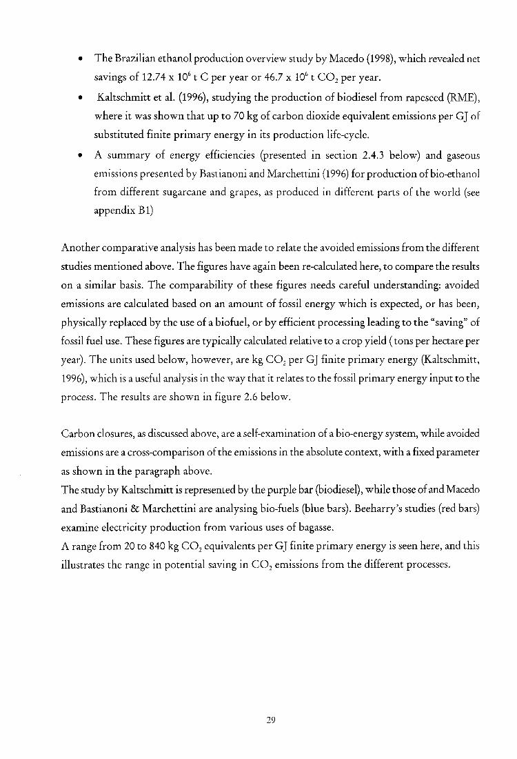
• The Brazilian ethanol production overview study by Macedo (1998), which revealed net

savings of 12.74 x 106 t C per year or 46.7 x 106 t CO2 per year.

• Kaltschmitt et al. (1996), studying the production of biodiesel from rapeseed (RME),

where it was shown that up to 70 kg of carbon dioxide equivalent emissions per GJ of

substituted finite primary energy in its production life-cycle.

• A summary of energy efficiencies (presented in section 2.4.3 below) and gaseous

emissions presented by Bastianoni and Marchettini (1996) for production of bio-ethanol

from different sugarcane and grapes, as produced in different parts of the world (see

appendix B 1)

Another comparative analysis has been made to relate the avoided emissions from the different

studies mentioned above. The figures have again been re-calculated here, to compare the results

on a similar basis. The comparability of these figures needs careful understanding: avoided

emissions are calculated based on an amount of fossil energy which is expected, or has been,

physically replaced by the use of a biofuel, or by efficient processing leading to the "saving" of

fossil fuel use. These figures are typically calculated relative to a crop yield ( tons per hectare per

year). The units used below, however, are kg CO2 per GJ finite primary energy (Kaltschmitt,

1996), which is a useful analysis in the way that it relates to the fossil primary energy input to the

process. The results are shown in figure 2.6 below.

Carbon closures, as discussed above, are a self-examination of a bio-energy system, while avoided

emissions are a cross-comparison of the emissions in the absolute context, with a fixed parameter

as shown in the paragraph above.

The study by Kaltschmitt is represented by the purple bar (biodiesel), while those of and Macedo

and Bastianoni & Marchettini are analysing bio-fuels (blue bars). Beeharry's studies (red bars)

examine electricity production from various uses of bagasse.

A range from 20 to 840 kg CO2 equivalents per GJ finite primary energy is seen here, and this

illustrates the range in potential saving in CO2 emissions from the different processes.

29

900 methanol from grapes (~aly)

800 • Biodiesel from RME

>- o ethanol from sugarcane (Louisiana)

~ 700 CD Delectricity from bagasse (common c w practice) ~ 600

Dethanol from sugarcane (Florida) .. E o electricity from bagasse (whole cane) .;: c.

~ 500 methanol from sugarcane (Brazil: Bastianoni c

& Marchetini , 96) ;;:::: ..., ~ electricity from bagasse (baled residue) C) 400

~ ~ethanol from sugarcane (Brazil :

:I Macedo,97) C" 300 ~ electricity from bagasse (com posted CD N 0 U CI

200 ... 100

0

Figure 2.6 Avoided emissions for different bioenergy systems

2.5.3 Energy efficiencies of bioenergy systems

The ratios relating energy output of the resultant bio-fuel to the fossil energy input into its

production are also key in determining the sensibility of making a particular product. The data

from the key studies in the previous discussions of this chapter again provides an excellent

comparison basis here, and the figure below shows the range of energy ratios realised in the

different systems. The figures reported in this chart have been sourced from the following

references: Ethanol from sugarcane for Florida and Louisiana, and from grapes in Italy - ref.

Bastianoni & Marchettini, 96; Biodiesel from soybean, and petroleum - ref. Sheehan et aI., 98;

Ethanol from maize in North America - ref. Berthiaume et aI., 01.

30

10 n----------------------------r---------------------------------

9

8 --::J Co 7 I:

S ~ 6 -::J o

- 5 o -CO ... 4 >-m ... CI) 3 I: CI)

.;;; 2 III o -

@grapes (Italy)

• petrolueum diesel

• ethanol from maize (N. America)

[J sugarcane (Louisiana)

• biodiesel from soybean

o sugarcane (Florida)

~ sugarcane (Brazil : Batianoni & Marchettini, 96)

~ sugarcane (Brazil: Macedo,97)

Figure 2.7 Fossil energy ratios

Fossil energy ratios below and in the region of 1 indicate no or low energy profit.

Only one of the bioenergy systems illustrated above (bioethanol from grapes) reports a fossil

energy ratio below than one, indicating no benefit in its production. The rest of the systems show

ratios of up to 9, indicating that encouragingly high energy yields are attainable in biofuel

production. The figure for petroleum diesel has been included here as a comparative measure.

2.5.4 Concems raised about bio-fuels

There are several environmental issues, however, in the production and processing of bio-fuels,

and these need to be highlighted and addressed before large-scale production of these fuels can

be advocated.

2.5.4.1 Land use

Key concerns in bioenergy production have been identified as its competition with food and fibre

production for land use and the removal of nutrients from the soil (Sims, 1999).

31

In support of this, the emergy analysis by Bastianoni and Marchettini (1996) to assess the feasibility

of bioethanol production (see section 2.4.2) found that th,lt one of the major constraints on the

feasibility of commercial cultivation of biomass for ethanol production was its competition for

arable land with food production. This is related to region'll population and per capita

consumptiOn.

A study by Marrison and Larson (1996), however, evaluated the potential biomass energy

production in Africa by 2025, in competition with land needs for food production. It was

concluded here that, with improved yield efficiencies for food cropping, even with only 10% of

land that is not forest, wilderness or cropland used for biomass energy crops, up to 18 EJ per

annum of bioenergy could be harvested, while meeting the needs of the population in terms of

food crops.

2.5.4.2 Gaseous emissions from use of biofuels

Although biofuels illustrate a general reduction in toxic emissions release, the analysis by

Kaltschmitt et al. (1996) identified poor results for nitrous oxide emissions in the use of bio-diesel

from rapeseed methyl ester. This result is confirmed by the findings of Sheehan et a1. (1998),

where biodiesel nitrous oxide emissions reported a 13% increase in comparison to petroleum

dieseL

In the modelling by Kadam (2002) of the use of an ethanol-gasoline blend (see section 2.5.1.1), it

was also shown that the blended gasoline has reduced comparative air emissions, with the

exception of nitrous oxide.

All hydrocarbons, with the exception of methane, were grouped together to investigate the

comparative severity of these emissions in the ethanol-gasoline blend, compared against normal

gasoline use. These hydrocarbons included volatile organic hydrocarbons (VOCs), ethanol,

furfural, hydroxymethyl furfural (HMF), aldehydes, and benzene. Here it was seen that the fuel

blend scenario produced 17% more hydrocarbon emissions compared to pure gasoline use.

2.5.4.3 Transportation

Another concern which is raised at times is the high energy requirement and environmental

burden of transportation of large volumes of low enere;y density of biomass fuels (Sims, 1999).

A relevant study was carried out for the exportation of bio-electricity from Scandanavia to

Holland.

The scenarios explored were the transportation of the solid biomass via different transportation

options (including road and sea), exportation of grid electricity after it is produced locally, and

domestic use of the electricity, without exportation. The results, however, showed no large

differences in environmental loads between any of the scenarios. Transportation of large volumes

of processed biomass fuel may thus have less significance in terms of comparative environmental

burden. The analysis here, however, involved combinations of road and sea transportation

options (Forsberg, 2000).

2.6 Conclusion of relevant literature

The following conclusions can be drawn from the discussions presented in this chapter:

• The renewability of biofuels can be assessed using carbon balances, energy yield

calculations and measures of fossil energy use in its life-cycle. Land use for crop

production in competition with its use for growing food crops is also a key assessment

parameter for determining the sustainability of the production cycle.

• Ethanol can be produced from a wide range of bioenergy sources, and various novel and

existing technologies are available for the different conversion routes.

• Carbon closures of above 90%, and up to 100% percent have been achieved for

sugarcane bio-energy systems. Energy yields of above 1, and up to 9 are also achievable,

in the context of bio-ethanol produced for sugar crops.

However, this range of results for different bio-energy systems, and in particular for bio­

ethanol, indicates that significant differences exist in the production schemes. This affirms

the hypothesis and approach taken for this study, in stating that there is need to assess the

specific dynamics of the production of bio-ethanol from sugarcane molasses as it is

currently done.

• The production and use of bio-ethanol as a gasoline additive replacement is potentially

feasible, and is superior to current gasoline use from an environmental perspective, in the

categories of resource and primary energy use, and some gaseous emissions. There is

33

concern, however, over the nitrous and sulphur oxide emissions from the gasoline

blended with ethanol.

• Although past studies show that bio-systems achieve overall energy and greenhouse gas

emission benefits, no studies have been done for South Africa, particularly for the

production of ethanol from sugarcane molasses.

34

3. GOAL AND SCOPE OF THE LIFE CYCLE ASSESSMENT

As laid out in the introductory chapter, this thesis centres on a cradle-to-gate life cycle assessment

of the production of bio-ethanol from sugarclne molasses in an industrial African setting, aiming

to compile a comprehensive inventory of all material and energy resource needs and its

environmental outputs, The details of this inventory are to be used to provide an indication of

the sustainability of providing this product, by determining the environmental impacts of the

collective of industrial processes harnessed.

The chapters to follow hereon are structured in line with the ISO 14040 standards on life-cycle

assessment methodology, where the following stages of a study are defined:

Goal and scope definition

Inventory Analysis

Impact Assessment

Interpretation

This chapter addresses the first of these stages, where the goals of the research into the life-cycle

assessment of ethanol produced from molasses are presented. The limitations on the scope of the

study, as well as details on the data quality and other parameters involved at the onset of the study

are also described,

However, before formally stating the goals and scope of the LCA, the thesis hypothesis shall be

revisited, as it is the main aim of the LCA to gather and interpret the necessary data to either

substantiate or refute this hypothesis.

3.1 Statement of hypothesis of study

The following hypothesis is re-stated for the production of bio-ethanol from sugarcane molasses:

The production of bio-ethanol from sugarcane molasses is principally a sustainable

process, based on the renewable nature of the sugarcane raw material. Life-cycle

assessment can be used to profile the environmental burdens of the production, and

identify areas of concern that are the focus of possible improvement.

35

Building on the conclusions of the literature review, this hypothesis can now be expanded.

Specifically, it is expected that the analysis of the bioethanol production life-cycle can show the

following technical points:

• A high carbon closure illustrating the sequestration of fossil carbon dioxide released during

conversion and use by that absorbed during biomass growth.

• A high fossil energy ratio, based on its self-sufficiency in energy requirement provided by

bagasse incineration and potential electricity generation.

• Competitive land use, allowing for simultaneous food and energy crop production.

• Concern over the emissions of noxious gases, such as nitrous and sulphur oxides, and volatile

hydrocarbons, which need to be acted on to reduce adverse local and regional impacts.

3.2 Goal of study

The primary goals of this study were:

• to generate a life cycle profile of ethanol as produced by the fermentation of molasses, a

by-product in the South African sugar industry, and

• to develop an understanding of the sustainability of the overall process and product, and

classify the extent of "environmental friendliness" of the product ethanol by determining:

(a) the carbon closure of the bioethanol product system,

(b) the fossil energy requirement for the cradle to gate life cycle,

(c) the environmental impacts of the resource use and emissions from the process.

36

Secondary objectives were to carry out this study so that it can complement other environmental

decision-making at the producer level, particularly:

• to record data at the distillery in such a way that it is of use in the design and

implementation of an environmental management system envisaged for the production

site; and

• to structure the data gathering at the molasses to ethanol process site so that it supports a

current project to design and implement an adequate waste management strategy for the

liquid effluent generated there.

Target Audience

This research was undertaken in fulfilment of the Master of Science in Chemical Engineering

degree awarded by the University of Cape Town. The initial target audience is hence an academic

one, including staff and post-graduate researchers in the field of Environmental Engineering and

Life Cycle Assessment. Researchers working on the bio-product are also part of the targeted

audience.

Secondly, the results of this study are intended for the use of technical management of the

sponsoring sugar company to aid their full understanding of the environmental issues associated

with their products, both existing and new. Subsequently, this information shall assist in decision

and policy making in the implementation of environmental management.

Finally) the data gathered in the study is to aid in assessing the environmental desirability of using

such bio-ethanol as a gasoline additive. Hence, this information also targets policy-making bodies

as well as commercial investors, as it may provide a basis for understanding the implications of

the production and use of the product as fueL

37

3.3 Scope

The following scope was proposed for the LeA at its outset:

3.3.1 System definition and boundary

The system to be studied is the production of ethanol by a sugar company. From the life-cycle

perspective, the system essentially involves the conversion of carbon dioxide and water into

glucose in biomass, most of which is extracted into the sugar process, with the remainder being

subsequently fermented to produce ethanol as the product of interest. The cradle of the study is

hence the growth of the sugarcane, and the gate end is the ethanol product from the distillation

process of the molasses-to-ethanol process.

The system to be studied is thus explicit! y defined as a process system, and the relevant sub-systems

consist of cane growing, cane processing (to separate molasses), fermentation (to produce

ethanol), and finally distilling of the ethanol-water mixture.

The following assessment shall hence be made, with regards to the system boundary:

• Sugar cane shall be traced back to its cultivation,

• The product ethanol out of the distillery shall be the final life cycle stage analysed,

excluding product use,

• Imported utilities and materials, such as electricity, coal, lime, sulphuric acid, fertiliser and

diesel shall be added into the study as closed loop flows, their production being analysed

using a relevant database profile.

The sub-processes for the life cycle shall hence be labelled as follows:

Agricultural Process (cane growing)

Road transport 1 (from cane fields to sugar mill)

Sugarcane to molasses processing

Road transport 2 (from sugar mill to distillery)

Molasses to ethanol process

Smaller process flows (not shown in the diagram) such as fertiliser for the Agricultural Processing

stage, and other process chemicals shall be evaluated for their contribution to the overall life

38

cycle. If deemed to be insignificant Qess than 0.2% of functional unit, on a comparative basis) to

the overall analysis they shall be left as open loop flows, and hence not included quantitatively in

the life cycle.

It is acknowledged that the sugarcane to molasses process exists predominantly for the

production of sugar. A formal allocation procedure (see section4.1) will be developed to account

for its share of the environmental burdens.

The diagram below illustrates the system boundary chosen for this study, in line with the

objectives defined and the goals:

t I Lime I production

Agricultural Sulphuric acid

------- processmg production

1 Sugarcane Road sugarcane to molasses Transport .. Molasses to ethanol ~

molasses Road 1---+

Processing 2 process fthanol

Transport 1

i I

Diesel I I

------------------1-----------------------sugar

J I Y Electricity ~ t

I Coal I t -_ ... _--------I mining I

Figure 3.1 System boundary for the life-cycle study

The dotted line illustrates the system boundary for the life-cycle study.

3.3.2 Impact categories to be studied

The following impact categories have been selected to be relevant to the analysis of the

environmental burdens of this product's life-cycle, and shall be investigated. For those impact

categories that are global in nature, emissions occurring outside the geographical area of the

production sites as a result of activities occurring within the system boundary will also be studied.

1. Global warming

2. Acidification

3. Nutrient enrichment

4. Impacts of land use

5. Photochemical ozone creation potential

6. Human toxicity

7. Ozone depletion

8. Resource depletion

The relevance of each of the impact categories listed above shall be made in the relevant

chapter (Chapter 6), with reference to the flows of interest, once the inventory has been

completed and presented. Their selection at this point is based on literature indications of the

aspects of bio-energy systems that are of environmental concern.

3.3.3 Functional unit

The functions of the product are multiple, each being specific to the particular market to which it

is supplied. The producer's interest lies primarily in the product's capacity for value generation.

The primary market to which the product is sold is the potable alcohol market, but in view of the

goals of the study, the product's recipient environment is variable. The function of the process

system can thus be defined as to produce ethanol product for use in its different target markets.

An amount of 1000 litres (1 kl) of ethanol shall be used as the functional unit for the study. All

data for mass and enf'~gy balances shall hence be normalised for this functional unit.

40

3.3.4 l)ata qluzlity

The quality of the data to be used in the study shall be based on the sugar company's current

production profiles. Average data values over a seasonal ethanol production period, and its

corresponding sugar processing season's data shall be considered sufficient to meet the goals of

the study.

An average scenario approach shall be used for the initial consideration of the variability of

process parameters used in the analysis.

A further approach shall then be employed in context of a sensitivity analysis, to determine the

response of the system in different cases of input and production variations, and with respect to

the allocation methods employed.

3.4 Concluding remarks

The goals and scope of this life-cycle assessment have been presented in this chapter, and the

sub-processes that constitute the life-cycle of bio-ethanol have been grouped. These process units

shall now be described in more detail in chapter 4.

41

4. Unit descriptions and inventory preparation

Proceeding from the goal definition for and the delimitation of the scope of the LeA presented

in chapter 3, this chapter now describes the important sub-processes making up the cradle to gate

life cycle, and discusses the methods used in acquiring and compiling the inventory data.

From a general identification and grouping of the sub-systems of the cradle to gate life-cycle, the

chapter proceeds to examine the allocation of environmental burdens between sugar and

molasses production. Each of the sub-processes of the life cycle shall then be described with

respect to its function, and the approach used to gather the relevant data is also outlined under

each sub-section.

The compilation of the data to produce a model of the process, and the use of software database

information is also discussed, and finally the quality of the data compiled is commented on.

In line with the definition of the system, its boundary and its sub-systems in section 3.3.1, it was

considered useful to group the sub-processes into those over which the company has a significant

degree of control (termed "foreground" processes, and those over which the company has little

control ("background" processes). Figure 4.1 shows the former in bold at the centre of the

system, and the latter supporting this primary production chain.

42

1 1 I Lime production I

I Sulphuric acid

I production

Road Agricultural Sugarcane Road -iM olasses to ethanol I operations

f- Transport i- to molasses Transport 1 processing 2 process ethanol

I - ~

sugar

Diesel production

I Electricity I t production I

I I t Coal .. _-_ .. I production r

Figure 4.1 Foreground and background sub-systems for the LeA

(a) Foreground sub-processes

These are the sub-processes related directly to the sites of production of the bio-ethanol, and are

directly associated with the processing of the product. These are:

• Agricultural Processing

• Sugarcane to Molasses Processing (Sugar Milling)

• Molasses to Ethanol Processing

• Road Transportation

Primary data, relating specifically to the production pattern and practices of the company in the

study, was compiled for these sub-processes (except Road Transportation).

Agricultural Processing is, strictly speaking, not under direct supervision of the Company, but

their exclusiveness as a cane buyer in the vicinity of the region puts them in considerable control

over the guality of the cane produced. It is hence deemed that they are both directly and

indirectly in control of the agricultural process.

Road transportation is classified as a foreground process, and is deemed to be partly under the

Company's supervision by virtue of the choice of transportation alternatives (e.g. rail) that the

producer would have, if it were found that this step had severe impacts on the environmental

profile of the bio-ethanol production.

(b) Background sub-processes

These are the sub-processes that involve the production of the ancillary flows of utilities and

reagents that are used in the foreground sub-process. It was considered sufficient to model these

processes using relevant published or software database information, due to the inaccessibility of

local primary data relating to them and the low degree of influence the company has over their

environmental profiles.

These background sub-processes are:

• Coal production

• Electricity production

• Lime production

• Sulphuric acid production

• Diesel production

• Fertiliser production

• Water extraction

It can be seen that the influence of the company on background processes would be minimal,

compared to that over the foreground processes. Medium influence on background processes

would imply that, by simply changing the source of the flow, the company could influence the

environmental burdens attached to the particular service it delivers. This is applicable only in the

event where the environmental burdens associated with the process were found to affect the

overall life cycle profile of the product under study in a detrimental manner.

The details of each sub-process will be illustrated in full in the subsections to follow, leading to

the data specifics gathered from each of the sites. Before this, however, it is necessary to resolve

the complications arising from the nature of the product (ethanol), as a by-product from another

production system, being that of sugar production.

44

4.1 Allocation

A methodological allocation problem arises when a multifunctional process has more than one

function for the product life-cycle under investigation, or a different function for other products.

In this case, it is a production process with two products, these being sugar and molasses.

The main product of the sugarcane to molasses sub-process is cane sugar, and molasses IS

classified as a by-product of this process. The molasses is often treated as a waste stream, but the

value addition of utilising this to produce ethanol is such that it can be considered as a by-product

stream. The problem is to decide what share of the environmental burdens of the specific activity

and its consequences should be allocated to the by-product investigated .

The system for which allocation is to be effected is the first section of the study as illustrated in

Figure 4.1 previously, isolated below for clarity:

r--------------------------------

Lime J

Agricu I tural

1 operations

sugarcane Sugarcane to molasses I

Road ~ Processing molasses -----. Transport

1

r I

Diesel

I r El .. I ectnctty I

sugar

Figure 4.2 The sugar-molasses co-production system

The environmental burdens associated with all the input Hows to this sub-process (electricity,

lime, diesel) and their associated inventory Hows, up to the production of the two products (sugar

and molasses) shall be affected by the allocation procedure to be adopted.

Allocation should ideally be avoided where possible either by expanding the system under

consideration, or by subdivision of the process to isolate the process routes which result in the

production of each of the individual products. However, in the event where the products are

made from the same process route, different approaches may be used to partition the associated

input and output burdens between them. Two criteria may be used to allocate between products,

these are technical and economic criteria (Ekvall & Finnveden, 2001).

Technical criteria relates to quantity and material grade of products, where as economic criteria

relates to the utility value of the products, and relative price becomes the partitioning key.

Allocation proportional to quantity and material grade can be used for co-products which arise

from the same material, as in this case (Hauschild & Wentzel, 1998).

Accordingly, a mass-based allocation shall hence be used to attribute fractions of the standard

input and output flows of this sub-process and of those preceding it, to the production of

molasses. A mass ratio of sugar product to molasses shall be used as the allocation factor for all

inventory inputs, outputs and calculations to be presented in the overall inventory.

Typically, a mass ratio of sugar to molasses of 3: 1 is expected, representing an allocation factor of

0.33 (Pillay, publication date unknown).

An alternative scenario to this is one where a11 inputs and outputs for the production of molasses

are attributed to sugar processing alone, on the basis that molasses is a waste product, and not a

by-product. This perspective is in accordance with the company's mission statement, which states

that the objective of their operations is predominantly for the production of sugar.

On this basis, the a11ocation to molasses has a factor of zero (0), hence molasses are regarded as a

"free" input with no environmental burdens. This assumption has, however, complications in the

defining of a carbon balance for the bio-ethanollife cycle, since the source of the molasses now

appears "untraceable".

The effect of this a11ocation sha11 be explored further in the context of a sensitivity analysis in

sections 5.7.1 and 6.2.10.

46

4.2 Major sub-processes

The unit processes invol ved in each subsystem shall be described in this section, together with

the details of the approach used to gather and compile the data relevant to each unit. Where

bound by confidentiality of the processing details, a generic description of the technology shall be

employed. The corresponding flows that are also of sensitive nature shall remain "masked" in the

inventory, but their associated environmental burdens shall be accounted for, in full.

4.2.1 Agricultural Processing Data

This is the sub-process in which the growing of the sugarcane is modelled, through to the cane

product as the key output from this stage. The different cane fields which supply the sugar

processing mill are all within an average distance of 30 km from the mill itself, which is situated in

the southern Kwa Zulu-Natal province of South Africa.

Based on the issues highlighted in literature concerning the cultivation of biomass for energy

production, and the goals and scope of this study, it was deemed sufficient to model the South

African cane processing profile based on the following key figures:

(i) Average cane yield per hectare (area-specific)

(ii) Fertiliser use per hectare (Nitrogen and Phosphorous fertilisers)

(iii) Water use for irrigation (where applicable)

(iv) Fossil energy use for machinery (predominantly diesel)

(v) Pesticides usage

Due to time constraints and unavailability of data, however, figures for pesticide use and water

for irrigation were excluded from the compilation of agricultural processing data. This is

considered as a significant discrepancy, because water is among the resources of concern in South

Africa, and the use of pesticides is also of note in the categories of toxicity (human and aquatic).

In general, however, the sugarcane growing practice in the southern region ofKwa Zulu-Natal in

South Africa does not involve irrigation, unlike the northern region where irrigation is common,

and the region reports very high water usage figures from the agricultural sector. Consequently,

the crop yields are higher for the northern regions than in the south.

47

The information used here was gathered from The South African Sugar Association via personal

communication (p. Govender), and the table below summarises the gathered estimates:

Table 4.1 A ricultural ~o~--csi~nLL------._ ... _~ __ ---c-_------,

'nput / Output nits

Fyield

iN fertiliser

Pfertilizer

on per ha

jkg per ha

Ikg per ha

60 -120

20-50

88 p,--)ie_sel_fu_e_l~. ___ ~_--,-l_it_r_es __ p_e~r_h_a_ --'-__ ... ___ . .-.1

4.2.2 Sugarcane to Molasses Process: Sugar milling data

This is the process where the sugarcane milling, and sugar and molasses production takes place.

The sugar mill studied processes sugarcane using conventional methods of cane crushing, juice

separation and concentration, and sugar crystallisation. There is a downstream process on site,

however, which utilises some of the bagasse to produce higher-value derivatives. The depleted

bagasse then returns to the sugar mill, where it is used as fuel for the boilers to produce process

energy.

The sugar milling operation can conveniently be grouped into 5 main process blocks:

• Milling & Extraction (cane cmshing and extraction of cane juice)

• Sugar Production (evaporation and crystallisation)

• Power Generation (electricity and steam generation)

• Effluent Processing & Handling

• Downstream Process (production of value-addition chemical)

The downstream process that uses bagasse to produce value-added products is mn as a separate

business operation, and hence it as relatively straightforward to allocate environmental burdens.

Figure 4.3 illustrates the site boundary described above, and indicates in general, the flows of

concern. The dotted line indicates the boundary of the study, and the flows shown to cross this

boundary are essentially the flows that are recorded in the inventory of this site.

Internal flows, such as the water and steam exchanges between the sub-processes are shown (in

blue), as well as the bagasse and fines flows (in brown).

r­I I I I I I I I I I

~ - - . I-Lime, flocculant, enzyme

Milling & Extraction

mixed juice

Sugar Production

- - - -cane

t---

<I.l ~ r/}

= <I.l "0 = 0 u

I bagasse

L - I-- - - - - - -suga r

molasses, filter cake

Legend

~ electricity

--~. water/ stearn! condensate

--.~ environmental flows

-

...., (1) r/}

§ = (1)

-

Figure 4.3 Sugarcane to molasses process

raw diesel ~ coal water - - -~ -. - - .,

Power Generation • • air ~ (inc!. water I emissions ,

treatment) I

ash

I dust

effluent I I sludge

J to swamp Effluent

~ I ::l Processing (1) Vl

& Handling Ro I air

_I emissions ,... - - - - -• • Downstream

J Process

Value products

The sections below briefly discuss the processes involved in the blocks illustrated in the diagram

above.

49

4.2.2.1 Milling & Extraction

This process step involves the crushing and shredding of raw cane, to separate the cane juice

from the fibre.

Inputs into this process block are cane, imbibition water, and steam, used to drive the shredders

and the cane knives. Imbibition water is an internal flow, its source being treated process water

from the clean water dam, a recycle stream.

The output inter-unit flows are the mixed juice, to the Main Process, and bagasse, which is an

internal flow to the downstream process, but returns as residue to the Power Generation to be

used as boiler fueL An environmental flow of concern here is dust, composed of bagasse fines,

from the cane handling, shredding and crushing. It is not normally monitored by the site

operation and thus could not be quantified in this inventory. It is a flow of concern, because it

can be harmful to human health and can cause a bronchial condition.

4.2.2.2 Sugar Production

This encompasses the boiler house operations of cane juice concentration by evaporation,

followed by crystallisation. The cane juice is heated to accelerate inversion, and the subsequent

evaporation procedures encourage crystallisation of the sugar crystals. Molasses are the

concentrate from a series of concentration processes. Notable inputs are lime, process flocculant

and enzyme. The main economic flows out of this process block are sugar, molasses and filter

cake.

The simplified figure below (figure 4.4) shows the sequence from which sugarcane and molasses

are produced in this process block.

Steam is used for heating to initiate evaporation, and then returns to the power generation sub­

process as condensate.

An important trade-off concept is observed here: the sugar processing aims to reduce the sucrose

content in its molasses to its minimum, to recover the most sucrose in its sugar product.

However, the molasses-to-ethanol process (to be discussed later) strives to attain the highest

sucrose content in its molasses to recover higher yields of ethanol product from its fermentation

process. There is hence the potential for the company as a whole to control and vary which of

their products, sugar or ethanol, is produced, and in what quantities.

50

syrup from Evaporators (86% sucrose) ;--__ oX-_-'---,

mixed

I Syrup

re-melting . -----1>1 (86% sucrose)

B-sllg.ar (92% sucrose)

C -sugar (83% sugar)

A-stage ~vaporation & centrifugation

A -sugar <)9.5 % sucrose

A-molasses (6X % sucrose) r--~--....,

evaporation & I'

ccntrifugatio!1 .

fillalmolasscs (34% sucrose)

Figure 4.4 Production of molasses and sugar: final stages

4.2.2.3 Power Generation

In this process block, high and low pressure steam is generated from the combustion of bagasse

in boilers. It is used to drive machinery, as well as turbo alternators to produce electricity, and to

provide process heat to the process and downstream sections. Other utilities, such as water and

wastewater management, as well as cooling, were considered part of this process block.

Diesel, coal and bagasse are the main economic inputs, while steam and electricity are the

economic outputs from this process. The environmental flows here are ash and air emissions

arising from the combustion of bagasse in the furnaces, as well as raw water intake and effluent

discharges.

Bagasse from sugar milling is produced in enough quantities to meet all energy requirements of a

sugar processing mill (Beeharry, 1999), hence it is assumed that the coal used in the boilers is for

the extra energy requirement of the downstream process. None of the coal used on site was

therefore allocated to sugar processing.

51

4.2.2.4 Sugar mill data compilation

The records for the 2000 production season of 44 weeks were compiled and aggregated, on a

weekly basis, to record the input and output values for the flows indicated in the discussions

above (See appendix Cl).

A simple combustion model calculation using a typical bagasse composition from literature was

used to estimate the gaseous emissions from the combustion of bagasse from the boilers. Finally,

average figures, as well as minima and maxima figures, representing the production profile over

the 44-week season were recorded.

4.2.3 Molasses to ethanol Process: Distillery Data

This sub-process and its associated background processes constitute the second half of the

overall LCA study, to form the complete cradle-to-gate picture of the process. This is shown in

the figure below:

I Lime I I Sulphuric acid

I ,- - - - - - -- f-------, , , , , I JM olasses to ethanol l

, I , I process I I

molasses , lethano , , , , ------- ----- - _ ...

I Electricity 1

" t ----·----------·--------····-·--·····--·--·--r Coal

Figure 4.5 Gate-to-gate profile of molasses-to-ethanol process

An assessment of the molasses-to-ethanol process block shall now be made to identify the key

processes, and the origins of the input and output flows recorded in the inventory for this site

process.

The molasses-to-ethanol process comprises of two main conceptual processes:

fermentation of the sugars present in molasses to alcohol

distillation, to separate the ethanol-water mixture

Similar to the sugar mill analysis, the site processes were grouped into sub-processes, depending

on their functionality, as follows :

• Molasses storage & handling

• Pre-fermentation

• Fermentation

• Distillation

• Steam & Electricity Generation

The figure below shows the site boundary for this process:

r­I I I I

- - -----,

creamed I

Molasses storage & handling

Steam & yea s t ---------1- -------------------------- E I e c tri cit Y

I r---~----,I+_--____1 G e n er a tio n

I I I I

dunder

Distillation

I I

I

I I

L __ _ _ _____ ....J

ethanol

Figure 4.6 Block flow diagram showing major distillery sub-units

dunder

4.2.3.1 Process description

This process follows conventional methods of ethanol production, as described in the literature

(section 2.3.1.5).

Molasses are stored in cone roof tanks, and are prevented from contact with moisture, to avoid

premature fermentation before they are introduced into fermentation tanks.

The use of cream yeast, however, is alternative to the pre-fermentation process which prepares

the yeast locally onsite, but this system was not operational during the period of observation.

The molasses are then introduced into the fermentation tanks where a batch fermentation

process takes place. They are first diluted with water to 25" brix because the sugars and salts exert

a very high osmotic pressure which would otherwise hinder the fermentation process. The

molasses originally have about 45% sugar content, which is reduced to about 14% after dilution.

The fermentation then takes place over approximately 30 hours, and some of the carbon dioxide

released is captured and sold as a separate product.

The "beer" from the fermentation process then undergoes a stripping process, where the dunder

is separated from the alcohol water mixture. The dunder is sent to waste tanks where

sedimentation of the solid particles takes place, while the liquid effluent is sent to sewage.

The ethanol-water mixture then undergoes a series of distillation processes, with a final ethanol

product of 95.4% purity (azeotropic point). Some absolute alcohol production may take place,

depending on requirement, and this is done by dehydrating the 95.4% ethanol product with

cyclo-hexane.

In the steam and electricity generation process, coal is used to generate 31 and 21 bar steam for

the distillation processes and other site requirements. Electricity can be generated using the high

pressure steam from the boilers to drive a turbine. In the period studied, however, there was no

electricity generation for the mills' internal use.

4.2.3.2 Data compilation procedures

An ethanol production period of 12 months, corresponding to the sugar production season for

which the sugarcane-to-molasses process data was compiled, was chosen for data gathering on

this process site.

Production figures over the studied period were obtained from the distillery operational records

to quantify the main economic flows, while the standard (environmental) flows were calculated

based on these flows, using results of sampling of wastes and emissions, which are recorded

54

periodically. The flows recorded were corrected to reflect the operation of the distillery only,

factoring out other commercial operations on site (a related mdependent production process

exists on site, and shares the utility requirements of the process studied here).

The approach used here was to compile month-by-month "black-box" mass balances over the

defined sub-units of the distillery, creating inventory lists of all inputs and outputs. The sub-units

were then inter-linked in sequence of the production line, to produce overall process profiles,

which were then aggregated to arrive at the one-year data inventory, and an average monthly one.

The collected data was compiled in a series of identical inter-linked Excel spreadsheets, one for

each sub-unit process, with a worksheet for each month. This matrix was summed to give an

overall profile of the process for each of the 12 months of the period of study, reflecting the

sums of all "economic" (purchased/sold) and "standard" (to or from the environment) inputs

and outputs for the studied system (see appendix C2).

4.2.4 Transportation Data

There are several transport steps involved in this life-cycle study. In principal, all transportation

of services and imported flows to the process should be included in the assessment. However, the

two steps of transportation directly involved with the manufacture of the product are the

following:

• Transportation of sugarcane from cane fields to the sugar mill (Road transport 1)

• Transportation of molasses from'the sugar mill to the distillery (Road Transport 2)

Based on the distance and load capacities involved with each of these, it was assumed that they

are the most intensive of the transport steps involved and would hence be the ones of most

significance,

Log book records of cane and molasses deliveries to each of the sites were used to determine the

average loads and truck capacities for deliveries, as well as the geographical locations of the

origins of each of the loads.

55

The transportation steps were modelled using LCI transportation databases, and the trucks used

are 40 ton and 30 ton diesel trucks, for the sugarcane and molasses transportation, respectively.

The return trip for the trucks is inclusive in the assessment.

The information gathered is summarised in the table below:

T bI 42 S a e f ummary 0 transportatIOn d ata Destination average average truck capacity other detail

load (tons) distance (km) (tons)

from cane field 30 30 40 diesel

to sugar mill truck

from sugar mill 30 70 30 diesel

to distillery truck

4.3 Ancillary units and model compilation

To incorporate the associated production inventories of other flows into the inventory of the

cradle-to-gate study, and for the evaluation of an environmental lmpact assessment,

environmental processing evaluation software was used.

The TEAMTM software by Ecobilan / Pricewaterhouse Coopers (PWC) was used to model the

entire cradle-to-gate life cycle process. Besides its availability, this software was determined to be

ideal for its ease of use, its extensive database for the production of several inputs that are

relevant to this study, and good impact assessment and valuation methods.

4.3.1 Interlinking of software modules and process data to produce overall inventory

The following software database modules were used, in addition to the compiled process data

described in the sections above:

• Coal Production

• Electricity Production

• Lime Production

• Diesel Production

• Sulphuric Acid Production

• Road Transportation

56

The inventories associated with each of these modules constitute cradle-to-gate life-cycle analyses.

However, there is need for precaution in using database information to model life cycles of

products, because the information on the software may penain to production patterns in Europe

and America, but may not necessarily reflect local production in South Africa.

With the exception of Electricity Production, whose database information has specifically been

modified to reflect the 1996 South African electricity production, the rest (coal, diesel and lime)

are generic production profiles. It is expected that a major discrepancy would be with respect to

energy use in such production steps, because European industrial production often has natural

gas as a key energy source, whereas in South Afnca, coal is the key energy source due to its

abundance and low cost.

Another possible discrepancy is the old technology used in industry in Africa, compared to the

technology on which these production modules are based.

A fertiliser production module was not available, and the approach below is proposed for the

determination of the relevance of its inclusion in the life cycle study.

4.3.2 Dealing with Fertilizer Production in the life-cycle inventory

In the LeA modelling package used, no databases were available for Nitrogen and Phosphorous

fertilisers used in the agricultural processing stage. The basic calculation approach shown below

proposes how to determine the significance of including this module in the overall inventory.

Assuming that Nitrogen fertilisers can be represented by Ammonium Nitrate (NH4N03), and

Phosphorous fenilisers are Ammonium Phosphate (NH4),PO.), the equations forthe production

of ammonia, subsequently the production of the fertilisers, are represented by the following

formulae:

Ammonia Production:

(1)

Ammonium Nitrate Production:

(2)

57

Ammonium Phosphate production:

3NHJ + H3PO .. <=> (NH,j)3 PO .. (3)

Based on these equations, and the fertiliser requirements for the agricultural stage, the

corresponding amount of ammonia required can be calculated.

Domene and Ayres (2001) have published emissions from the production of ammonia using

natural gas obtained from an Aspen simulation of the process (see table 4.3 below). An

adaptation for the production of the ammonia required for the fertilisers can be made to simulate

those emissions corresponding to the production of the required amount of ammonia.

The CO2 emissions can then be used as an indication of the energy intensity of the process, using

the a rough estimation that the fertiliser production step is as energy intensive as the modelled

ammonia production.

This figure can then be compared to the fossil COl reporting in the final inventory, and the

significance of this production step can hence be deduced. This analysis is applied in section

5.7.2.2 to follow.

Table 4.3 Emissions from ammonia production value per 1000kg NH3

Inputs Air 15109 CH4 I 615 H2O 11000 Outputs CO2 1500 N2 10900 I H2S in I

(Domene and Ayres, 2001)

4.4 Overall data quality evaluation

Evaluation of data quality i~ important for understanding the reliability of the data gathered, and

also for the correct interpretation and use of the results. The section above has already described

the adaptability of software data for use in this life-cycle analysis.

58

4.4.1 Temporal and technological representation

The use of primary data from specific sites means that the production profile resulting from the

analysis is specific to the analysed site. However, both the sugar milling and molasses-to-ethanol

processes are generic, and follow conventional production methods. It is hence deemed that the

results of this life-cycle analysis can be confidently used as an indication of current procedures

and methodology in this industry, for the specific region.

The gathered data are for the production season for the year 2000 - 2001.

4.4.2 Data consistency

The methods of data aggregation for each of the site processes have been described in their

respective sub-sections previously. Weighted averaging was used to arrive at the aggregates

recorded for the overall production profiles, over the 44 weeks of production for the sugarcane­

to-molasses process, and over 12 months production, for the molasses-to-ethanol process.

Data checks on unreasonably high or low numbers were made, and extreme outliers were

excluded in the averaging procedure.

The periods of operation studied for the sugarcane-to-molasses and molasses-to-ethanol

processes were consistent with each other, to avoid seasonal variations in crop yield and sucrose

content, which would otherwise off-set the material balances on which the inter-linking of the

processes is based.

The figures for the agricultural operations, however, are not very accurate, and can be considered

as first-order estimates to create an understanding of the associated key input and output values.

4.5 Conclusion

Each of the sub-processes involved in the life cycle has been described, and the key flows into

and out of them have been highlighted. The corresponding data aggregation procedures have also

been described, and the raw data for these c:an be found in appendix B. The augmented

inventories for the ancillary flows which have been obtained from a software database have also

been listed, and together these make up the cradle-to-gate inventory, which shall now be

presented and discussed in the chapter to follow.

59

5. RESULTS AND INTERPRETATION OF INVENTORY

5.1 Introduction

Using the methods of compilation and modelling described in chapter 4, the full LeI was

compiled, and is shown in appendix A.

In this chapter, the basic material balances for each of the site processes analysed are first shown,

leading to the presentation of a brief summary of the appendix A. Some key input and output

flows are highlighted here, leading to their discussion.

An interpretation of the inventory is then presented, starting with a comparison of the

foreground and background process, from an energy and material perspective, and leading onto

the determination of life-cycle performance measures similar to those found in the literature.

Finally, an analysis of different factors which affect the inventory is made, referring to the system

allocation, as well as other flow and modular changes to the system.

5.2 Material balances for the main processes

The details of each of the site processes have already been discussed in section 4.2, under the

approach used for data gathering. The diagrammatic representations of the processes illustrate the

key inputs and outputs to each process, to create an overall picture of the material flows involved

on the production of the final ethanol product.

5.2.1 Agricultural Operations process data summary

The diagram below summarises the economic flows for data gathered at the process level for the

Agricultural operations, normalised for the production of 1 ton sugarcane:

60

Nitrogen fertilizer

Phosphorous fertilizer 0.47 kg

diesel 1.2 kg

Land use 133 m 2

Agricultural Operations

sugarcane 1 ton

Figure 5.1 Material inputs and outputs for Agricultural operations

..

This cane now feeds into the Sugarcane to Molasses process, as discussed under section 4.2.

5.2.2 Sugarcane to molasses Process data summary

For this process, there are two different material balances, one for the combined sugar and

ethanol system, and the other corresponding to a mass allocation of the burdens of sugar

processing to the production of molasses alone.

In the first analysis (figure S.2a), the material balance of the overall process is shown, where sugar

and molasses are the main products, and the relative inputs and pertaining to their production are

shown. Figure S.2b shows the allocated figures for the production of molasses only, the sugar

output is hence considered to be zero in this scenario.

61

sugarcane 26 tons water 9.7 kl

lime 15.4 kg

Sugarcane to molasses

Process I

molasses J ton

tons tons I

..

Figure 5.2a Sugarcane to molasses Process data (without partition between products)

Bagasse is an internal flow, consumed in the process stage, and hence does not appear as an

output from this process. This illustrates the performance of the overall bio-energy system;

sugarcane is converted to molasses and sugar. The process flows have been normalised for the

production of 1 ton of molasses.

The effect of the partitioning between these two products can now be seen in figure S.2b to

follow.

62

sugarcane

4 kg

Sugarcane to molasses

Process

molasses I ton

filter cake : 0.4 tons liquid effluent: 0.08

Figure s.2b Sugarcane to molasses Process data (with allocation to molasses production)

For every ton of molasses produced, 2.8 tons of sugar are also produced. Based on the discussion

in section 4.1 on allocation, the allocation factor for partitioning between sugar and molasses

production thus becomes 1 equals to 0.26. This means that 26% of the sugar processing (1 + 2.8)

burdens is allocated to the production of molasses alone.

The comparison of these two figure S.la and S.2b clearly shows the effect of allocation; in figure

S.2b appropriated values for inputs and output values for the production of molasses alone are

shown, as though the process was solely for the synthesis of this product. The significance of this

allocation on the carbon balance becomes evident here; 1 ton of molasses is produced from 26

tons of sugarcane in the overall process, yet only 6.8 tons of this cane is appropriated to the

production of the molasses alone.

The alternative zero allocation of burdens to molasses production would mean that no inputs and

outputs are assigned to this flow, hence the molasses flow becomes the cradle of the study. The

effects of this shall be explored further in section 5.6.1.

63

5.2.3 Molasses to ethanol Process data summary

The molasses produced from the previous process stage are now processed at the distillery to

produce ethanol.

Similar to the previous analysis, figure 5.3 below summarises the operation of the distillery. Here

the flows are normalised for the production of 1 kl of ethanol product

1 rno asses

Molasses ethanol water to ethanol •

16.2 kl 1 kl Process

s ulphuric acid . 3.8 kg

Alcohol by-products : 0.04 kl Ii uid effluent q .21. 1 4 CO2 product : 0.11 tons

Figure 5.3 Material inputs and outputs for Molasses to ethanol Process

These three sub-processes and the associated background processes previously described form

the overall bio-ethanol production life cycle, which is now presented in Table 5.1 to follow. This

table is an abridged form of appendix AI, and only shows the flows for the 26% allocation

system, highlighting the flows of interest which are discussed in the sections to follow. The reader

is referred to appendix A for a full perusal of the complete inventory.

64

TABLES.1 : ABRIDGED INVENTORY FOR BIOETHANOL PRODUCTION SYSTEM. WITH 26% ALLOCATION TO MOLASSES PRODUCTION

Flow Units TOTAL Coal Diesel Sulphuric Acid Lime Electricity Road Agricultural Molasses to Sugarcane to Production Production Production Production Production Transport Processing ethanol process molasses process

Inputs: (r) Coal (in ground) kg 1.46E+03 1.31E+03 5.07E-03 1.42E-02 1.07E-02 1.46E+02 (r) Limestone (CaC03, in ground) kg 6.ooE+Ol 1.23E+OO 1.03E-02 3.46E+Ol 2.41E+Ol (r) Natural Gas (in ground) kg I.S6E+Ol 9.43E+00 1.07E+OO I.S2E-Ol 2.4SE+OO 2.S0E+00 (r) Oil (in ground) kg 4.92E+Ol 2.35E+00 4.63E+Ol 377E-02 t07E-Ol 4.22E-Ol (s) Nitrogen (N) 9 1.01E+04 1.07E+04 (s) Phosphorus (P) g 2.39E+03 2.39E+03 Land Use (II -> III) m2a 5.59E+00 5.59E+OO 6.90E-05 1.49E-07 land Use (II -> IV) m2a 7.48E-Ol 7.48E-Ol 8.40E-OS 1.81E-07 Land Use (III -> IV) m2a 3.S4E+03 2.6SE-Ol 9.S2E-OS 2.0SE-l0 3.S4E+03 Water Used (total) mre 2.96E+04 2.19E+03 1.90E+02 9.56E+00 6.68E+00 3.09E+02 1.62E+04 1.07E+04

Outputs (a) Aromatic Hydrocarbons (unspecified) 9 1.79E-04 610E-OS 3.I9E-07 8.16E-l0 1.18E-04 (a) Carbon Dioxide (C02, biomass) 9 7.86E+06 7.S0E+05 7.11E+06 (a) Carbon Dioxide (C02. fOSSil) 9 2.26E+06 6.83E+04 1.29E+04 5. 1 OE+02 21SE+04 2.40E+05 499E+04 1.87E+06 (a) Carbon Monoxide (CO) 9 7.85E+03 6.3SE+02 B.l0E+00 7.16E-02 3.41E+00 3.10E+02 t36E+02 6.76E+03 (a) Ethanol (C2H50H) 9 S.OOE+03 9.21E-05 4.61E-06 1.14E-05 209E-04 8.00E+03 (a) Hydrocarbons (except methane) 9 5.29E+02 1.09E+02 309E+02 2.61E+00 4. 17E+Ol 6.66E+Ol (a) Hydrocarbons (unspecified) 9 I.S5E+Ol 9.10E+OO 2.8SE-02 5.25E+00 1.31E-03 1.10E+00 (a) Lead (Pb) 9 2.67E-Ol 6.30E-02 3.0SE-03 9.89E-05 1.9SE-Oj S.51E-03 (a) Methane (CH4) 9 8.46E+03 7.36E+03 2.23E+02 9.49E+00 8.66E+02 2.04E+00 (a) Nitrogen Oxides (NOx as N02) 9 3.7SE+04 6.24E+02 3.14E+Ol 2.96E+OO 7.08E+OO S.54E+02 6. 39E+02 1.50E+03 3.41E+04 (a) Nitrous Oxide (N20) 9 1.00E+Ol 4.64E-Ol 1.42E-Ol 2.34E-02 2.74E+00 6.99E+00 (a) Organic Matter (unspecified) 9 2.74E-02 U5E-02 7.36E-04 1.S9E-06 9.21E-03 (a) Particulates (unspecified) g 3.41E+03 1.21E+03 6.63E+00 6.81E+00 2.96E+02 1.86E+03 347E+Ol (a) Sulphur Oxides (SOx as S02) 9 1.48E+04 3. 16E+02 6.S1E+Ol 7.75E+Ol 1.80E+00 1.23E+03 7.97E+OO 4.62E+03 S.S2E+03 (w) Acids (H+) 9 2.74E+Ol 3.S9E-01 7.63E-04 2.66E+Ol 2.24E-05 4.34E-02 3.70E-Ot 1.07E-05 (w) AOX (Adsorbabte Organic HalogenS) 9 1.02E-02 4.S9E-04 9.66E-03 2.2BE-05 5.7BE-05 (w) BOD5 (Biochemical Oxygen Demand) 9 9.96E-Ol 2.20E-02 2.07E-Ol 7.60E-Ol 3.49E-03 3.79E-03 (w) Chlorides (CI-) g t47E+04 1.11E+04 2.35E+03 5.78E+OO 1.2SE+03 (w) COD (Chemical Oxygen Demand) 9 1.39E+06 3.49E-Ol 6.84E+00 5.4SE-05 S.11E-02 5.07E-02 1.39E+OS S.90E+00 (w) Dissolved Matter (unspecified) 9 2.70E+OS 8.17E+02 1.5SE-Ol 4.S6E-02 9.S1E-OS 9.18E+Ol 2.69E+OS 5.34E+02 (w) Dissolved Organic Carbon (DOC) 9 S.67E-02 1.7SE-03 1.42E-02 4.05E-02 2.9SE-04 (w) Nitrates (NOS-) 9 7.23E+00 S.24E-Ol 6.83E+00 1.S2E-02 606E-02 (w) Nitrites (N02-) g 1.28E-05 3.9SE-07 3.21E-06 9. 14E-OS 6.S4E-08 (w) Phosphates (P04 3-, HP04--. H2P04-. HSP04. as P) 9 6. 22E-04 5.19E-05 1.03E-04 2.9SE-04 1.72E-04 (w) Phosphorus (P) 9 2.00E-02 9.00E-04 I.S9E-02 5.49E-OS 1. 14E-04 (w) Sulphates (S04--) g 1.14E+OS 4.49E+02 3. 79E+Ol 3.77E-Ol 7.83E+Ol 1.13E+05 (w) Suspended Malter (unspecified) g 6.30E+05 1.38E+Ol 1.0BE+00 2.2BE+00 2.53E+OO 263E+OO 8.30E+05 5.05E+00 (w) VOC (Volatile Organic Compounds) g 1.68E+00 7.56E-02 1.59E+00 3.43E-03 9.S9E-03 (w) Water (wnspecified) litre 1.26E+03 1.11E+03 2.70E-03 S.63E-06 1.42E+02 (w) Water: Chemically Polluted litre 2.14E+04 1.20E+01 7.79E+00 1.6SE-02 1.62E+OO 2.14E+04 sugar product tons 1.19E+Ol 1.19E+Ol ethanol product kl 1.00E+OO 1.00E+OO Waste (Iotal) kg 4.96E+02 4. 17E+02 1.93E-OI 1.82E-02 2.45E-03 8.ooE+Ol 3.41E-Ol

Reminders: E Feedstock Energy MJ 2.34E+04 2.09E+04 1.88E+03 1.20E+01 2.93E-02 1.28E+03 -6.80E+02 E Fuel Energy MJ 4.32E+03 2.81E+03 9.08E+Ol -1.16E+Ol 1.05E+02 6.S0E+02 6.80E+02 E Non Renewable Energy MJ 2.77E+04 2.37E+04 1.97E+03 3.S5E+00 1.05E+02 1.92E+03 E Renewable Energy MJ 1.28E+Ol 9.34E-Ol 8.41E-03 5. 17E-04 1.74E-02 1.19E+Ol E Total Primary Energy MJ 2.78E+04 2.38E+04 1.97E+03 3.85E+OO 1.0SE+02 1.93E+03

5.3 Discussion of key inputs and outputs

5.3.1 Resource inputs

Coal and oil represent the key primary energy inputs into the life cycle. The mass of each resource

input per kl of product made is shown here, but a more effective scmtiny of primary energy input

can be made with respect to the particular background sub-processes from which each of the

resource uses originate, as shown in Table 5.2 below:

T bI 52 E a e nergy va ues 0 f resource mputs Flow Units!TOTAL Coal Diesel ISulphuric ILime Electricity Sugarcane

acid I to Production Production I Production I Production Production Molasses

Process (r) Coal (in ground) kg 1455.6 1309.8 0 0 0 145.8 0 (r) Oil (in ground) kg 49.2 2.4 46.3 0 0.1 0.4 0

(r) Natural Gas (in kg 15.6 9.4 1.1 0.2 2.5 2.5 0 ground) Bagasse kg 4320 0 0 0 0 0 4320

E Total Primary MJ 27758 23751.6 1966.9 3.9 105.2 1930.2 0 Energy (fossil) !

E Total Primary MJ 31622 0 0 0 0 0 31622 Energy (biomass)

The natural gas recorded here refers to coal bed methane; the table above shows that 9.4 kg of

the reported 15.6 kg total for natural gas (in ground) originates from the Coal Production sub­

process, confirming this.

It is interesting to note the comparative energy value of bagasse. This value is not reported in the

overall inventory, since it is an internal flow, but has been shown here to illustrate the energy

contribution that the biomass plays in the overall process. Based on the LHV Oower heating

value) of bagasse, it has a 1.1 times higher primary energy value (31,600 MJ) than the total fossil

energy input (27,800 MJ), and this is for the allocated scenario. This illustrates the magnitude of

biomass energy available from the sugar process, and justifies the assumption that all energy

requirements of the process can be satisfied, in excess, by the use of bagasse.

For the fossil energy inputs, the following points are noted:

• The overall fossil primary energy distribution is dominantly attributed to coal production

(86%), while Electricity (7%) and diesel (7%) production share the remainderfraction.

66

It can be seen here that lime and sulphuric acid production are relatively insignificant to

the overall life-cycle, on an energy basis,

This enforces the point raised previously that coal usage is the key fossil energy

contributor.

• Of the non-energy inputs (Table 5.1), water use is 29,600 lines for every 1000 lit res of

ethanol product, and this is without accounting for cane irrigation.

5.3.2 Gaseous emissions

Biomass carbon dioxide (7.9 tons) and fossil carbon dioxide (2.3 tons) are the main gaseous

emissions, while nitrogen oxides, sulphur oxides, carbon monoxide, methane and ethanol vapour

contribute 37kg, 15 kg, 8kg, 8kg and 8kg respectively. The dominance is clearly on the part of

carbon dioxide emissions. These flows are the key to several of the impact categories to follow in

the subsequent chapter.

Particulate emissions are also significant under the human toxicity impact category; here the key

particulate emissions {3.4 kg} originate from the Coal and Electricity production sub-processes.

However, the particulate emissions from the primary processing sites (particularly bagasse from

sugarcane to molasses process) were unquantified and hence this figure represents an

underestimation of the particulates emitted in this life-cycle.

5.3.3 Water emissions

The following water emissions immediately stand out as significant, from the life cycle:

sulphates (502') (116 kg), chlorides (Cn (16 kg), dissolved matter (270 kg) and suspended matter

(830 kg), The effluent also reports a chemical oxygen demand (COD) of 1390 kg, and together

these flows are of significant impact depending on their recipient environment. This effect shall

be described further under the relevant impact categories in the chapter to follow (Chapter 6).

It should also be noted that scenarios such as accidental pipe failure, leading to leakage of water

emissions into aquatic ecosystems, have not been assessed. The impact of these emissions largely

depends on whether they are emitted to a waste treatment plant, or directly to aquatic eco­

systems.

67

The subsections to follow shall now present different interpretation aspects of the results which

have been presented in sections 5.2 and 5.3.

5.4 Comparing foreground and background sub-process

An analysis of the relative intensities of the foreground and background processes on the

inventory is made here. This is done to determine how much influence the producer can have on

the overall environmental profile of the bio-ethanollife-cycle.

Isolating which flows, and subsequently which environmental impacts are a result of the primary

process of production, and those which are secondary from the inventories associated with the

imported flows does this.

The list in Table 5.3 focuses on those flows which have a contribution from both the two

mentioned classes of sub-process, and a percentage analysis is used here to determine the

emphasis of the foreground sub-process on the totals for these flows reported in the inventory.

The following overall assessment can be made for the relative impacts of the foreground and

background process:

• Foreground processes dominate the use of land, due to agricultural processing land use for

cane growmg.

• Water usage is largely (90%) attributed to foreground processes, without the values for

lrngatlOn water.

• Gaseous emissions of carbon dioxide (fossil and renewable), carbon monoxide, ethanol

vapour, nitrogen oxides, nitrous oxides, and sulphur oxides are dominantly from the

foreground processes.

Particulate emissions are however noted as being dominantly from background process, and

this is because those from foreground process were unquantified (section 5.3.2 above). The

total shown here is clearly an underestimation; foreground processes would be expected to

dominate the emission of particulates as they do with gaseous emissions.

• Emissions to water of COD, dissolved and suspended matter, and sulphates are fully

attributed to foreground process, and in particular to the molasses to ethanol process.

• The total waste (solid waste) reported here (500 kg) is chiefly mining tailings from Coal

Production. However, there is a large amount of ash from the molasses to the ethanol

68

process which was not quantified, which would affect the balance of contribution between

foreground <md background processes, for a mass of 0.75 tons of coal consumed.

The background processes hence account for the majority of the input and output flows by

fraction of mass, but the few flows which are dominated by foreground process are actually of

key value to the several impact categories, to be discussed in the chapter to follow.

This is important information, because these emissions are very significant for several impact

categories to follow in the subsequent chapter, and this shows that the company can have direct

influence on these angles of the overall environmental profile (see discussion in section 4.3).

It should be noted again here that air emissions mainly originate from the combustion of coal and

bagasse in the foreground processes producing molasses and ethanol, respectively.

Water and land use were also isolated as significant resource inputs into the life cycle, and the

analysis here confirms that these are also within the company's influence to reduce their impact.

69

Table 5.3 Comparing foreground and background sub-processes

Flow Units Life Cycle Total Background Foreground % contribution of Processes Processes foreground processes

Inputs Land Use (III -> IV) m2a 3.84E+03 2.65E-01 3.84E+03 100.0 Water Used (total) litre 2.96E+04 2.71E+03 2.69E+04 90.9

Outputs (a) Benzene (C6H6) g 7.54E+00 7.53E+00 1.59E-02 0.2 (a) Benzo(a}pyrene (C20H12) g 4.02E-02 4.01E-02 7.94E-05 0.2 (a) Cadmium (Cd) g 8.86E-03 8.07E-03 7.92E-04 8.9 (a) Carbon Dioxide (C02, biomass) g 7.86E+06 O.OOE+OO 7.86E+06 100.0 (a) Carbon Dioxide (C02, fossil) g 2.26E+06 3.43E+05 1.92E+06 85.0 (a) Carbon Monoxide (CO) g 7.85E+03 9.57E+02 6.90E+03 87.8 (a) Ethanol (C2H50H) g 8.00E+03 3.17E-04 8.00E+03 100.0 (a) Hydrocarbons (except methane) g 5.29E+02 4.62E+02 6.68E+01 12.6 (a) Lead (Pb) g 2.67E-01 2.64E-01 3.51E-03 1.3 (a) Methane (CH4) g 8.46E+03 8.46E+03 2.04E+00 -(a) Nitrogen Oxides (NOx as N02) g 3.75E+04 1.22E+03 3.63E+04 96.7 (a) Nitrous Oxide (N20) g 1.04E+Ol 3.37E+00 6.99E+00 67.5 (a) Particulates (unspecified) g 3.41E+03 3.38E+03 3.47E+Ol 1.0 (a) Sulphur Oxides (SOx as S02) g 1.48E+04 1.69E+03 1.31E+04 88.6 (a) Zinc (Zn) g 2.35E+00 1.91E-01 2.16E+00 91.9 (w) Acids (H +) g 2.74E+01 2.70E+Ol 3.70E-Ol 1.4 (w) COD (Chemical Oxygen Demand) g 1.39E+06 7.29E+00 1.39E+06 100.0 (w) Dissolved Matter (unspecified) g 2.70E+05 9.09£+02 2.70E+05 99.7 (w) Sulphates (S04--) g 1.14E+05 5.66E+02 1.13E+05 99.5! (w) Suspended Matter (unspecified) g 8.30E+05 2.24E+01 8.30E+05 100.0 (w) Water: Chemically Polluted litre 2.14E+04 2.14E+Ol 2.14E+04 99.9 Waste (total) kg 4.98E+02 4.98E+02 3.41£-01 _ 0.1

5.5 Environmental performance indicators for the Molasses to

Ethanol Process

A specific focus of this assessment is the molasses to ethanol process. This is revisited

here in line with the classification made in the introduction to Chapter 4, where this

process is classified as one on which the company would have the high influence, with

respect to altering its environmental performance for improvement.

To characterise the environmental profile of the distillery, the use of average indicators

for each of the nine key inventory flows is proposed, calculated from the inventory.

These indicators represent four input parameters (molasses, coal, water and electric

power), one internal one (steam use) and four representing outputs to the environment

(fossil and renewable carbon dioxide, sulphur dioxide and liquid effluent).

Table 5.4 lists the values calculated to be the average load during the 1-year study period.

Table 5.4 Eco-indicators (Flows per kilol itre of product alcohol) I Indicator Units Value i

. Coal ton/kl 0.75 I

I Water kllkl 16.4

I Power kWh/kl 251

Steam GJ/kl 16.2 i

I CO2 (fossil) ton/kl 1.89

I CO2 (renewable) ton/kl 0.75

S02 kg/kl 4.4 I

I Effluent kllkl • 22.3 !

It is seen that approximately 2.65 tons of carbon dioxide (total) are produced, and three

quarters of a ton of coal consumed for every kilolitre of product.

Water use (16.4 kllkl) also appears to be high, for a fermentation-distillation process.

Further, there is an obvious imbalance here, of water input versus total effluent (22.3

kllkl). During the data gathering exercise, it was reported that water input flowmeters

71

were faulty. It is therefore recommended that further observation of water use be made

for this site process to determine a more accurate input figure.

Electricity is imported onto site. It is interesting to compare this to the analysis by

Beeharry (1999), which showed that up to 58 kWh per ton millable cane can be produced

at sugar mills. Since110 tons are processed per kl of product, this means that up to 6.4

GWh/kl electricity is potentially available for export from sugarcane processing. This is

greater than the reported 251 k Whl kl requirement for this site, and prompts the

possibility of the use of "green" electricity, produced elsewhere by the same company,

from residual biomass.

5.6 Life cycle performance measures based on inventory data

In this sub-section, some of the life-cycle calculations described in section 2.4.1 of the

literature review are performed on the inventory data, and a comparative analysis of the

figures attained here is made with those found in the literature. The focus here is on

carbon flows and energy inputs and outputs associated with each of the sub-processes.

5.6.1 Carbon analyses of the bio-system

In the analysis of bio-energy systems, it is imperative to track all the key carbon flows

associated with the biomass, to determine the efficiency of the conversion process,

overall. Figures 5.4a and 5.4b illustrate this, the biomass carbon flows are shown in

green, while additional carbon flows (fossil fuel use) to the system are shown in brown.

The overall bio-energy system's performance from a carbon perspective is made, paying

attention to the accounting of carbon over each of the sub-processes. The carbon

closures of the allocated and unallocated systems are then compared and the parallels

between the two scenarios are drawn.

5.6.1.1 Process carbon balances

Figure 5.4a shows the bioenergy system without partition of process inputs and outputs,

where the system represents the simultaneous production of both sugar and molasses,

corresponding to the production profile shown previous] y in section 5.2.2 and figure

5.2a.

In this overall bio-energy system analysis, the following carbon balances are observed

over individual sub-processes:

• Over the sugarcane-to-molasses process, sugarcane is converted to molasses, bagasse

and sugar product. A carbon balance over this process achieves a closure of 98%.

• The molasses-to ethanol process, however, shows a carbon balance closure of 84%

only, for the flows recorded here. This discrepancy here is seen for the following

mam reason:

5.6.1.2

Ounder (waste from the fermentation process) is rich in carbon, which may not

have been fermented to ethanol. This accounts for most of the carbon which is

lost to waste here, the high readings of suspended (830 kg) and dissolved matter

(270 kg) from the molasses to ethanol process illustrates this. Assuming a 10%

carbon content in the combined suspended and dissolved matter represents 0.11

tons of the unaccounted 0.12 tons of carbon here.

Other possible carbon losses may be from other alcohol products (pure ethanol,

and low grade (industrial), which are not tracked in this analysis, and product

vapour losses from the distillation process, which were estimated at 1 % of the

final product. These, however, are insignificant in comparison to carbon losses in

dunder.

Carbon closures for the bio- energy system scenarios

The concept of carbon closure has been discussed previously in section 2.4.1 and is now

revisited here. Carbon closure is defined by the formula

where B,C and 0 refer to the carbon in CO2 emissions from fossil energy use in the

agriculture and harvesting, transportation, and conversion stages of the biofuel

production respectively, and A refers to the carbon fixed in the biomass during

photosynthesis (growth). It is essentially an indicator for the extent of fossil CO2

mitigation which a system is allowed by the fixing of carbon into biomass during growth.

73

The numbers denoted "B", "C"(I.2) and "D"(t.2) refer to the fossil carbon inputs to the

different stages in the life cycle. An assumption shall be made here, that all the carbon in

these fuels shall be converted to CO2 during combustion. This is an assumption; in

practice the efficiency of combustion would be such that less carbon would be released

as CO2, hence the carbon closure calculated here represents the minimum value

attainable.

"A" denotes the carbon in the biomass (sucrose and fibre), while "E" is the carbon in

the final ethanol product.

Applying the formula above to the figures shown in the combined sugar-ethanol system

shown in figure S.4a, a carbon closure of 94% is achieved. This means that, as an overall

operational system, the off-set caused by fossil carbon dioxide release to the atmosphere,

to the carbon fixed in biomass during its growth is only 6%, and this represents a

relatively good performance of the system.

Figure S.4b is the corresponding carbon analysis for the illustration in the previously

shown figure S.2b, where 26% allocation to the production of molasses only is made.

Only the inputs and outputs to the cane growing and sugarcane to molasses processes are

affected by this allocation procedure, as can be seen in the figures on this diagram.

The carbon closure achieved for the bio-ethanol system is now only 79 %. The

difference between the carbon closure of the combined sugarcane-ethanol system (94%)

and this figure is significant; this is a clear indication that the production of molasses only

to produce bio-ethanol in the current context of the sugar manufacturing process has

poor performance in terms of fossil carbon emissions.

5.6.2 Fossil energy ratio

This analysis now relates the fossil energy inputs to the energy value of the final output

product, as opposed to the carbon closure, which related fossil carbon emissions to the

carbon input.

With reference to figures S.4a and S.4b again, the fossil energy ratio is then the energy

value of the ethanol E, weighed against the energy value of all the fossil energy inputs

together ("B", "C" (1,1) and "D" (1,1)) (see section 2.4.1.2) The formula is repeated here for

clarity:

74

Fossil energy ratio = EE I (EB + Ec + ED)' (accounting for fossil energy inputs only)

where Ex is the energy value of the flow in the diagram.

Fossil energy ratios of 1.06 for the combined sugar-ethanol system, 1.13 for the 26%

allocation to molasses production and 1.14 for the zero allocation to molasses production

scenario are realised (see appendix B2).

The combined sugar-ethanol system ratio is calculated here simply for comparison, of

importance is the figure corresponding to the 26% allocation scenario. This ratio (1.13)

indicates that the renewable energy harvested in the ethanol is marginally higher the total

fossil energy requirement for its retrieval.

This figure remains relati vely the same for the zero allocation scenario (1.14) because the

coal input alone is equivalent to 86% of the energy recovered in the fuel product, and is

unaffected by the allocation between the two products (sugarcane and molasses). This

shows that the fossil energy intensity of the molasses-to-ethanol process is the key

determining factor for the overall yield outlook for the entire system.

Application of the discussion in section 2.4.1.2 is made here; this figure illustrates how

the energy benefit of the product bio-fuel matches the fossil energy input into its

production. In this context then, the process appears not sustainable.

75

A CO 2 captured product =0.03 ton C

E

9.7 tons C

1 kl Ethanol =0.42 tons C

D2 0.52 ton C

B · 1 Cane growing (coal) ·1 Molasses to ethanol 0.042 ton C ( diesel)

C1 0.0025 ton C (diesel)

110 tons cane =9.7 tons C

process 0.2 ton C L-_____________ ,..---.Jrfermen tation

Dl 4.81 E-4 ton C (diesel)

molasses 0.77 ton C

carbon dioxide

Sugarcane to molasses process

13.6 ton CO 2

bagasse combustion =3.7 ton C

4.26 ton molasses =0.77 ton C

12 ton sugar =5 ton C

C2 0 .011 ton C ( diesel)

Figure 5.4a A carbon analysis of the combined sugar-ethanol bio-system

A

2.52 tons C

D2

CO 2 captured product =0.03 ton C

E 1 kl Ethanol =0.42 tons C

B · 1 Cane growing 0 .52 ton C • (coal) I Molasses to ethanol

0.011 ton C (die sel)

c} 6 .5E-4 ton C ( diesel)

process 0.2 ton C

D} 1....-_________ --, .. _-----1. fe rm en t a ti 0 n

28.8 tons cane =2.52 tons C

1 .25E-5 ton C (diesel)

Sugarcane to molasses process

3.5 ton CO 2 bagasse com bustion = l.0 ton C

molasses 0.77 ton C

4.26 ton molasses =0.77 ton C

C 2

carbon dioxide

0.0 11 ton C (diesel)

Figure 5.4b A carbon analysis of the bio-energy system with 26% allocation to molasses

•

5.7 Analysis of factors which influence the bio-ethanol inventory

There are several factors which affect the inventory, and subsequently the environmental

profile of the study.In this section, the effects of allocation on the inventory shall first be

explored, followed by an analysis of the sensitivity of the inventory to other variations

such as the influence of including a fertiliser production module and a coal transportation

module. Finally, a discussion on the use of toxic substances in the processing of the

alcohol is presented.

5.7.1 Effect of allocation on bio-ethanol inventory

As described in section 3.3.1, a mass-based allocation has been used to accordingly

attribute the resources and burdens of molasses production in parallel with sugar

production.

In the alternative scenario, an allocation factor of zero is made with respect to molasses

production, which effectively implies that molasses are a "burden-free" input into the

life-cycle. The argument here is that the essence of the sugar milling process is to

produce sugar, as informed by the company's mission statement, and molasses are simply

a waste product stream which may not be allocated for. The molasses flow becomes the

"cradle" of the study, and the ethanol product out of the distillery is the "gate" end of

the study.

This excludes the Agricultural processing and Sugarcane to Molasses sub-processes, and

road transport (to sugar mill). The figure below shows this modified system:

78

r------------------------------

I Lime production I

I

Road

Sulphuric acid production

-------, • .-----1----------+1 Transport _____ Molasses to ethanol t-_--=-_____ •

molasses 2 process

Diesel production

I Electrici ty 1t--___ ----1f _____ -'----. production I ...

i Coal L. ___________________ .______________________________ pro d u c ti 0 n

Figure 5.5 Modified system with zero allocation to molasses

5.7.1.1 Effect of allocation on primary energy requirements

ethanol

From an energy perspective, the effect of attributing none of the sugar processmg

burdens to the production of molasses can be shown by comparison to the original

scenario where 26% of the burdens have been allocated. The table below shows these

figures, and the discussion follows below:

T bl 55 E a e 1 . £ 11 nergy analysIs or una ocate dlli I e eyc e Flow Units TOTAL Coal Diesel Sulphuric acid Lime

Production Production Production Production E Total Primary Energy MJ 26275 23752 575 4 27 (zero allocation) E Total Primary Energy MJ 27758 23752 1967 4 105 (26% allocation)

79

Electricity Production 1917

1930

The following observations are made:

• The total primary energy remains relatively unchanged (5% change), and this

confirms that the energy intensity of the life cycle is focused on the Molasses to

Ethanol process, and its related background processes.

• Coal and sulphuric acid production figures remain unchanged, as these pertain

specifically to the molasses to ethanol process. Electricity production is slightly

reduced, to correspond with the exclusion of the lime and diesel for the detached

sugarcane to molasses process, and the related transport step.

• Diesel Production shows the biggest reduction for the scenario with no allocation

to molasses production, since the upstream agricultural, transport and sugarcane

to molasses processes have the higher requirement for this utility.

It should be noted here that these changes may have more significant impacts than

identified here, and shall therefore be re-investigated under the impact assessment

sections in the following chapter.

The resulting inventory with zero allocation to molasses can be seen in Appendix A2.

5.7.1.2 Other notable flows affected by allocation

From the analysis above, it can be seen that the standard flows associated with diesel,

lime and electricity production are changed accordingly due to the effect of the

allocation. In particular, noxious gas emissions associated with diesel and electricity

production will be significantly reduced in the scenario with zero allocation to molasses.

However, the significance of these changes can be seen best in the context of the impact

assessment which follows in the next chapter.

Other significant flows affected by the allocation are the following:

• land use is now excluded (see Appendix A2) from the life-cycle.

• water use is reduced by 37%.

80

5.7.2 Sensitivity of the bio-ethanol study to the inclusion of other sub-processes

5].2.1 Influence of the transportation steps

The two transport steps, which have been analysed in this bio-ethanol study, are the

transportation of sugarcane from agricultural fields to the sugar milling site, and that of

molasses to the distillery site. Table 5.6 below shows the energy intensities of each of

these steps:

Table 5.6 Relative intensities of the two trans nergy Capacity

M tons

~S49 40 30

olasses transportatio 1131 • 0 distille .

30 70

It can be seen here, that for a zero allocation to molasses, the first transportation step

becomes excluded, and the combined energy intensity of the transport step is decreased

by 80%.

The overall intensity of the transport step (680 MJ) is relatively insignificant, compared to

the combined energy intensity of the other sub-processes (27758 MJ) in the analysis of

the subsections above, and this shows that this may have no significant impact on the

inventory.

However, the largest imported flow is coal to the molasses-to-ethanol process; 0]5 tons

of coal are consumed per kl of ethanol produced. This coal is mined in an area

approximately 300 km from the production site, and is shipped by rail transport. This

step has not been added to the analysis of the overall process.

A separate model of this transportation step was made, in comparison with the transport

steps which have been discussed above, and the following results were found:

The coal transportation step has an energy intensity of 47.5 MJ fuel energy, compared to

the total value of 678 MJ fuel energy for the two transport steps currently included in the

study.

This would represent a 7% increase in the energy intensity of the life-cycle transport step

overall, should it be included in the analysis. But the analysis above also showed that the

81

existing transportation sub-system has a primary energy value of only 2% of the

combined energy intensities of the other sub-processes.

It appears then, that the omission of the coal transportation step may not have an impact

on the overall transport energy requirement for the process and other associated flows.

Nevertheless it remains a recommendation that an update of the process model should

include all transportation steps of imported process flows, as these may collectively have

significant bearing on the environmental profile of the study.

5.7.2.2 Effect of including fertiliser production data

As pointed out in section 4.3.2, the unavailability of data for the production of fertilisers

resulted in its exclusion as a sub-process module. However, the section proposed an

analysis method to determine the extent of influence that this sub-process may have on

the overall inventory. The basic approach is repeated here for clarity, and the following

results were found:

Assuming that Nitrogen fertilisers are represented by Ammonium Nitrate (NH4N03),

and Phosphorous fertilisers are Ammonium Phosphate (NH')3P04)' the following

calculation can be made:

Ammonia Production:

Ammonium Nitrate Production:

Ammonium Phosphate production:

3NHJ +H)P04 <=> (NH.).1PO./

(1)

(2)

(3)

Now, usage figures are 90 kg/ha and 35 kg/ha for the Nitrogen and Phosphorous

fertilisers respectively (see section 4.2.1). For a cane yield of 75 tons/ha, and an allocated

production figure of 28.8 tons cane per functional unit, using equations 1,2, and 3 above:

82

Allocated fertiliser input

Ammonium Nitrate (NH4NO,): ~~ (28.8) = 34.6kg

From equation (2), using molecular ratios, the amount of ammonia required is:

17 80 (34.6) = 7.3kgNH)

Ammonium Phosphate (NH4).\P04: ~~ (28.8) = 11.5kg

Using equation (3), this amounts to

~(11.5) = 4kgNH1 149 '

The total amount of ammonia required to produce these fertilisers is 11.3 kg NH3 per

f.u. (functional unit).

Domene and Ayres (2001) have published emissions from the production of ammonia

using natural gas which were obtained from an Aspen simulation of the process. These

are adapted for the production of the 11.3 kg ammonia required per functional unit as

follows:

Table 5.7 Emissions from ammonia production (adapted for calculation) value kg • per 1000kg per f.u I NH,

Inputs •

Air 15109 170.9 !

CH4 615 6.9 H2O 11000 124.3 Outputs CO2 1500 17.0 N2 10900 123.2 H2S 13 0.1

Focusing on CO2 emissions alone to determine energy intensity of the process, an

estimated factor of 2 was applied to account for the energy intensity of the actual

fertiliser production process of equations 2 and 3. The figure for CO2 emissions becomes

34 kg per f.u.

83

The inventory reports a CO2 (fossil) total of 2320 kg per f.u. 34 kg hence represents

about 1.4% of total emissions, when included in the total.

At this level of contribution it would be more appropriate to include the fertiliser

production steps into the bioethanollife cycle, especially as emissions of some pollutants

(e.g. nitrous oxides) might be higher in relative terms. However, given the lack of access

to a suitable appropriate database, fertiliser production has been excluded here.

5.7.2.3 Use of toxic chemicals for alcohol production

Cyclo-hexane is used as a dehydrating agent to produce absolute alcohol (100% ethanol)

from the azeotropic mixture of the final distillation product (see section 4.2.3). However,

it was not recorded in the inventory, hence an investigation into the extent of its use was

launched.

It was found that only 0.36 I cyclo-hexane per kl of ethanol product is used in the

production life-cycle, representing 0.04% of the functional unit. On the basis of the rule

used to exclude associated primary processing flows, which excludes all flows that

represent less than 0.2 % of the functional unit, the exclusion of cycle-hexane and its

production in the life-cycle study is hence justified.

Nevertheless, the material safety data sheet (MSDS) for this substance indicates that it

flammable, as well as toxic to humans in the event of ingestion. It should therefore be

handled with extreme care and sensitivity, especially when using for processing alcohol

for potable use.

The exercise of this caution is also extended to the use of sulphuric acid, which is highly

corrosive, and is fatal if ingested into the body.

84

5.8 Concluding remarks for the inventory interpretation

From the interpretation of the inventory figures discussed here, it can be seen that:

• Coal Production accounts for 86% of the fossil primary energy input into the life

cycle, and Electricity and Diesel Production each contribute 7%. The solar energy

endowment, invested in the bagasse, is 1.1 times greater than the fossil energy

input.

• Foreground processes dominate the emission of many of the key environmental

flows.

• The overall ethanol-sugarcane production system has a carbon closure of 94%,

but the allocated production system shows a carbon closure of 79%.

The 26 % allocated system shows a fossil energy ratio of 1.13.

• A zero allocation to molasses only induces a 5% decrease in the fossil primary

energy requirement, compared to the 26% allocation scenario. Diesel requirement

shows the greatest change in resource use, when allocation is effected.

• Transportation, as a life-cycle sub-process, has only a 2% contribution to the

energy intensity of the overall process. The inclusion of Coal Transportation in

the inventory was shown to have little effect on the overall energy input

requirement.

• The exclusion of Fertiliser Production as a module in the life cycle was also

determined to be allowable if not optimal, based on an order of magnitutde

carbon analysis.

This chapter has presented the results of the life-cycle inventory, and has analysed

several of the indicators for the performance of the overall system. The analysis here,

however, is largely on a mass and energy basis; it is important to determine the

significance of each of the flows with respect to impact categories. The chapter to

follow (Chapter 6) does this, and the analysis is also used to identify if the changes in

85

the inventory discussed here have any significant impacts in terms of the effects

caused in the relevant categories.

86

6. LIFE CYCLE IMPACT ASSESSMENT

6.1 Introduction

This chapter discusses the different impact assessment categories used to evaluate the

results of the inventory.

One of the goals of this study is to determine a measure of the sustainability of the

production process. An indication of the sustainability of a production process can be

seen from the impacts that it has on the environment from which it draws its resources,

and to which it emits its environmental outputs.

There are also several scenarios presented in the previous chapter, which may have

shown insignificant changes in the mass and energy flows reported in the inventory, but

may have notable changes in the context of the impacts which they cause.

The impact categories that are studied here were presented previously, in section 3.3.2.

The impact assessment results were generated from the TEAM'" tool for impact

assessment, using the following methodologies for impact categories:

CML - Centre of Environmental Science, Leiden University

IPCC - International Panel on Climate Change

USES - Uniform System for the Evaluation of Substances

WMO - World Meteorological Organisation

CST - Critical Surface-Time, Ecole Poly technique Federale de Lausanne

The results have been presented in graphical form, showing the contributing flows for

the particular impact categories, corresponding to the different sub-processes from

which the particular flows originate.

87

6.2 Results from impact categories used to assess inventory data

The subsections to follow shall then discuss the individual impact categories and their

contributing sub-processes. All the results in this section are for the 26% allocation

scenano.

6.2.1 Climate Change

The sun's short-wave radiation (UV and visible light) is reflected directly or re-emitted

from the atmosphere, or the surface of the earth as longer wave infrared (IR) radiation.

A "natural" greenhouse effect is created due to the presence of water vapour in the

atmosphere, where the re-emitted radiation is absorbed in the atmosphere, maintaining

the earth's temperature. However, the emission of gases by man-made activities increases

the absorption of this re-emitted radiation, and is additionally increasing the earth's

temperature in a detrimental manner. The key pollutant gases in this respect are CO2

(carbon dioxide), CH4 (methane), NzO (nitrous oxide), and halocarbons (Hauschild &

Wenzel, 1998).

Figure 6.1 shows the results of the greenhouse effect potential of the overall life-cycle,

illustrating the contributions from each of the sub-processes, in units of g equivalent

CO2, The effect over 20 years is the category shown in the analysis here.

It can be seen here that the key contributors are CO2 and CH4• As foreseen, the molasses

to ethanol process' coal combustion releases the most CO2 over the entire life-cycle,

creating a greenhouse effect potential of 1870 kg equivalent CO2 ,

Coal Production is then the second key contributing process to this impact category,

releasing 540 kg equivalent CO2, The contribution of methane here is from coal bed

methane.

Electricity Production is the third key contributing process in this category.

88

6.2.2 Acidification

Soil, or aquatic ecosystems acidification is an impact which leads to the reduction in the

system's acid neutralising capacity, directly caused by the addition of hydrogen ions

which displace other cations which are in turn leached out of the system.

For a substance to be classified as acidifying, it should therefore be responsible for an

addition or release of hydrogen ions in the recipient system, where the accompanying

anions become leached from the system (Hauschild & Wenzel, 1998).

501, NOz and NHI are dominant in the inventory, and are the chief cause of this effect,

hence classifying this category as relevant to the study.

Figure 6.2 shows the results of this analysis. The combustion of bagasse in the sugarcane

to molasses process releases the most S02 and NOz, followed by the coal use of the

molasses to ethanol process.

The location of the Sugarcane to Molasses Process is such that the recipient environment

for air acidification would be the agricultural sector that produces sugarcane; the leaching

of soils as a result of acidification would possibly reduce the land fertility and marginalise

crop yields, or else require lime addition.

The Molasses to ethanol Process is located in an urban industrial area, and corrosion of

metal structural degradation would similarly become an issue of concern.

These results are in line with the predictions made from the literature survey, which

highlighted the emissions of SOl and N 0 1 as key in the life-cycle of bio-energy systems

(section 2.5.4.2). The analysis there was based on the use of the product fuel, whereas

here the cause is due to the incineration of the biomass during processing. Nevertheless,

the combustion of the bagasse is in the interest of energy recovery, hence it becomes a

relevant issue.

Another aspect of agricultural practice not analysed in this study is the practice of cane­

burning before harvest. This would also have significant implications for the

environmental profile of the Agricultural Process, producing effects similar to those

caused by the bagasse incineration of the Sugarcane to molasses Process as shown.

89

N 0 (.) -t: (1)

co .~ :l C'" (1)

C)

2~~'-------------------------------------------------------------------

1800000

I 1600000

1400000

1200000 I

1~

I

800000

I 600000

400000 +1----1

200000 +1 ------I

o Coal

Production

I

• • •

Diesel Sulphuric Acid Urne Electricity Road Transport Molasses to Production Production Production Production ethanol

Process

Figure 6.1 IPPC-Greenhouse effect (direct, 20 years) for bio-ethanollife cycle

I - (a) Carbon Dioxide (CO2, fossil)

- (a) Carbon Tetrafluoride (CF4)

I o (a) Halon 1301 (CF3Br)

I o (a) Methane (CH4)

- (a) Nitrous Oxide (N20) I

800

700

600

+ 500 ::I: .... c ~ ~ 400 :l C'" (1)

C) 300

200

100

o

r--

r--

r--

r--

r--

~ ; ..-

:~ -

-

--- - ~

Coal Production Diesel Sulphuric Acid Electricity Road Transport Molasses to Sugarcane to Production Production Production ethanol Process molasses

Process

Figure 6.2 CML-Air Acidification potentials for bio-ethanollife cycle

• (a) Ammonia (NH3)

• (a) Hydrogen Chloride (HCI)

o (a) Hydrogen Fluoride (HF)

o (a) Hydrogen Sulphide (H2S)

• (a) Nitrogen Oxides (NOx as N02)

(a) Sulphur Oxides (SOx as S02)

6.23 Nutrient Enrichment

The depletion of oxygen at the bottom of lakes and coastal waters is called

eutrophication. This is caused by the excess enrichment of the aquatic environment

with nutrient salts, particularly those of nitrogen and phosphorous, which leads to

excessive growth of algae and other plant life, which in turn consumes oxygen when they

are broken down. Subsequently, all aquatic life suffers the lack or reduction of oxygen

levels, leading to death (Hauschild & Wenzel, 1998).

In the agriculture subsystem of the process, N&P (nitrogen and Phosphorous) fertiliser is

applied to the fields and it is a reasonable assumption that a significant amount of the

fertiliser is run off into water streams, causing eutrophication. An estimation of this was,

however, omitted due to information limitations.

Similarly, the Sugarcane to molasses Process is located along a coastal margin, and

inevitably some effluent from the effluent lagoon seeps into the sea, but a figure of this

quantity is also not available. This is a significant shortfall in the inventory.

Of the recorded information, the COD (chemical oxygen demand) of the Molasses to

ethanol Process effluent is the most significant contributor to this effect (Figure 6.3).

A comparative assessment can only be commented on with the contribution of the

lacking areas discussed above, and so the results in this category can be classified

incomplete and require further analysis for meaningful interpretation.

6.2.4 Photochemical oxidant formation potential

Depending on climate conditions, air emissions from industry and transportation can be

trapped at ground level. Here they react with sunlight to produce photochemical smog,

which contains ozone, produced from the interactions of volatile organic compounds

(VOCs) and NOx in the following sequence:

L VOCs, CO and OH react in sunlight to form peroxy radicals.

2. The peroxy radicals oxidise NO to NO c.

3. N02 is split by sunlight with formation of NO and release of oxygen

atoms.

4. Oxygen atoms react with molecular oxygen (OJ, to form ozone, 0 3,

The hydrocarbons responsible for this phenomenon are the following, ranked in order of

decreasing potential:

Alkenes, aldehydes, ketones, alkanes and hydrocarbons (Hauschild & Wenzel, 1998).

A significant source of contribution to this category is the alcohol vapour emissions from

the distillation process of the Molasses to ethanol Process. An estimation of 1 % of

ethanol product lost to fugitive emissions was made, and this results in a higher

contribution than all other aspects of the life cycle (figure 6.4). Should the fugitive

emissions be found to be in the region of 0.1% of the functional unit, this would

represent a value of 32 grams equivalent ethylene, which would still be among the higher

values of those identified from the other sub-processes.

It is interesting to note the insignificance of the road transport sector in this life-cycle,

with respect to hydrocarbon emissions here.

93

- (w) Ammonia (NH4+, NH3, as N)

5

D(w) Nitrogenous Matter I 4 (Kjeldahl , as N)

D(w) Nitrogenous I 3 Matter (unspecified, as N)

- (w) (;2 Phosphates a. (P043-, .~ HP04--, :::s H2P04-, C"

G)

H3P04, as en

- rJ) 1

Phosphorus (P)

0

- (w) Pho_sphorus

-Coal

Production

n_ Diesel Sulphuric Acid Lime

Production Production Production Electricity Production

r--

~

Molasses to Sugarcane to ethanol molasses Process Process

Figure 6.3 CML-Eutrophication potentials for bio-ethanollife cycle

30000

25000

20000 0

(w) COD (Chemical

-Oxygen

15000 Demand)

- 10000

- 5000

o

350

300

250

G> c:::: G> 200 >.

.J::. .... G>

> ":;

150 0-G> Cl

100

50

o I Coal Diesel

Production Production Sulphuric

Acid Production

n • Lime Electricity

Production Production

I Road Molasses to

Transport ethanol Process

• (a) Acetylene (C2H2)

• (a) Alkane (unspecified)

o (a) Benzene (C6H6)

o (a) Butane (n-C4H1 0)

• (a) Butene (1-CH3CH2CHCH2)

1111 (a) Ethane (C2H6)

. (a) Ethanol (C2H50H)

D(a) Ethylene (C2H4)

. (a) Formaldehyde (CH20)

• (a) Heptane (C7H 16) D(a) Hexane (C6H14)

. (a) Hydrocarbons (except methane)

• (a) Hydrocarbons (unspecified)

• (a) Propane (C3H8)

• (a) Propylene (CH2CHCH3)

• (a) Toluene (C6H5CH3)

Figure 6.4 WMO-Photo-oxidant fonnation potentials for bio-ethanollife-cycle

6.2.5 Ozone depletion

This impact category is classically included in life-cycle assessment; however the

processes in this study do not release the responsible emissions for its cause, and hence

its relevance is suspected to be minimal.

The stratosphere is the region 15-50 km above the troposphere, which is the part of the

atmosphere above the earth for up to 10 km upwards. Here, the presence of ozone, 0 3,

is significantly higher than in other regions for the following reasons:

• Photolytic formation of ozone from oxygen under the influence of UV radiation,

• The relatively high stability of ozone in the bottom stratum of the stratosphere

A naturally occurring ozone depletion process occurs in this region in the presence of

methane, nitrous oxide, water vapour, and chlorine and bromine compounds.

Man-made activities have increased the release of chlorine and bromine-containing

componds: CFCs, tetrachloromethane, 1,1,1 - trichloroethane, HCFCs, halons and

methyl bromide. Resultantly this has increased the natural ozone depletion process,

exposing the earth to the harmful UV B-radiation from the sun, otherwise filtered by the

ozone layer.

The assumption that this effect is insignificant is confirmed by the result shown in figure

6.5. All the contributing process have emissions under 0.12 g equivalent CFC-11 over the

life-cycle, with Diesel Production having the highest contribution of 0.11 g equivalent

CFC-l1 per kl of ethanol produced. Normalised, this contributes 2.14E-10 ofthe global

impact, which is relatively insignificant, as shall be seen under the normalisation

discussion (section 6.3) to follow.

6.2.6 Human toxicity

This impact category is a complex one for evaluation because the number of substances

which contribute to it is very large, and there are different basic toxicity mechanisms such

as damage to DNA, induction of allergy or inhibition of specific enzymes. As a result,

there is no unanimity on any coherent and operational method for a quantitative

assessment of toxic substances, within the environmental assessment of products.

96

The following classification of toxins which affect human health is made:

• metals e.g. lead, cadmium, mercury, emitted from processes, causing various acute

and chronic effects.

• Persistent ~ow degradability) substances e.g. PCBs (polychlorinated biphenyls),

P AHs (polycyclic aromatic hydrocarbons) and dioxins, which accumulate in adipose

tissue.

• Organic substances which emulate the female sex hormone oestrogen on sensitive

receptors in humans and animals.

• Volatile organic compounds, sulphur and nitrogen oxides, as well as particulate

matter.

Direct exposure occurs via inhalation and ingestion, while indirect exposure can be

through ingestion of plants which have been exposed to pollution, or ingestion of

consumers of their products (e.g. herbivores) (Hauschild & Wenzel, 1998).

Several different methods of evaluation have been used to analyse this impact category,

to illustrate a range of concerns that arise from the different approaches. Firstly, the

assessment of two methods, USES and CST, are compared. The results are shown in

figures 6.6a and 6.6b.

The USES method (figure 6.6a), in units of grams equivalent 1-4 dichlorobenzene,

highlights the lead (Pb) emissions from Electricity Production (13.2 kg equivalent) and

Coal Production (4.2 kg equivalent), but also the nitrogen oxides from the Sugarcane to

molasses Process (8.9 kg equivalent).

The CST method, in figure 6.6b. focuses on the emissions from Electricity Production,

with Selenium as the chief pollutant. In figure 6.6c (CML method) the sulphur oxide and

nitrogen oxide emissions from the Molasses to ethanol and Sugarcane to molasses

Processes are highlighted as the key emissions of human health concern.

Overall, trace elements from coal fired power stations, nitrogen oxides and sulphur

oxides appear to be the key health issues arising from the life-cycle, in agreement with the

focus laid out in the opening paragraph of this sub-section.

97

0.12 ,------------------------------------------------------------------------------------------

0.1

0.08

""'" ""'" • () LL ()

0.06 .~ :::l C'" (1)

C)

0.04

0.02 +-----------------------------

o +------

Coal Production Diesel Production Lime Production Electricity Production

Figure 6.5 WMO-Ozone depletion potentials for bio-ethanollife cycle

CI) c CI) N C CI) .0 0 '-0 .c 0

" q I ,....

:> ·S C'" CI)

C)

14000

12000

10000

8000

6000

4000

2000

o J,.... ~

Coal Production

n l I Diesel

Production

1

U Electricity Production

FI n

Road Transport

-

-

-

-

rI Molasses to Sugarcane to

ethanol molasses Process Process

Figure 6.6a USES-Human toxicity potentials for bio-ethanollife cycle

- (a) Ammonia (NH3)

- (a) Arsenic (As)

o (a) Benzene (C6H6)

o (a) Benzo(a)pyrene (C20H 12)

- (a) Cadmium (Cd)

(a) Cobalt (Co)

- (a) Copper (Cu)

o (a) Lead (Pb)

- (a) Mercury (Hg)

- (a) Nickel (Ni)

D(a) Nitrogen Oxides (NOx as N02)

- (a) Sulphur Oxides (SOx as S02)

- (a) Vanadium (V)

- (w) Ammonia (NH4+, NH3, as N)

- (w) Benzene (C6H6)

- (w) Nickel (Ni++ , Ni3+)

3500

3000

2500

... ctS .!l 2000 a.. -c ~ ctS .~ ::::s 1500 C" Cl)

1000

500

o " r1IL l. • -- -- • Coal Production Diesel Production

. fl-Electricity

Production

- (a) Arsenic (As)

- (a) Cadmium (Cd)

D(a) Carbon Monoxide (CO)

D(a) Chromium (Cr III, Cr VI)

- (a) Cobalt (Co)

• (a) Copper (Cu)

- (a) Lead (Pb) D(a) Mercury (Hg)

-(a) Nickel (Ni)

- (a) Nitrogen Oxides (NOx as N02)

D(a) Particulates (unspecified)

- (a) Selenium (Se)

- (a) Sulphur Oxides (SOx as S02)

- (a) Zinc (Zn)

• - • • Road Transport Molasses to Sugarcane to

ethanol Process molasses Process

Figure 6.6b CST-Human toxicity potentials for bio-ethanollife-cyde

30000

25000

20000

C) 15000

10000

5000

o .,

Coal Production

Diesel Production

Sulphu ric Acid

Production

- ~ Electricity Production

• Road

Transport

I Molasses to

ethanol Process

-

-

Sugarcane to molasses

Process

Figure 6.6c CML-Human toxicity potentials for bio-ethanollife cycle

- (a) Arsenic (As)

- (a) Benzene (C6H6)

o (a) Cadmium (Cd)

o (a) Carbon Monoxide (CO)

- (a) Heptane (C7H16)

I- (a) Hydrogen Sulphide (H2S)

- (a) Lead (Pb)

o (a) Manganese (Mn)

- (a) Nickel (Ni)

- (a) Nitrogen Oxides (NOx as N02)

D(a) Sulphur Oxides (SOx as S02)

• (a) Vanadium (V)

- (a) Xylene (C6H4(CH3)2)

- (w) Barium (Ba++)

- (w) Xylene (C6H4(CH3)2)

6.2.7 Resource depletion

This impact category is of interest in evaluation; while the classification of the use of

metal ore as being non-renewable is questionable, based on our capability to recover and

recycle metals, the consumption of other resources such as crude oil, coal and natural gas

is definitely an irreversible process. The unit of measurement is "fraction of reserve", and

the results require careful evaluation, because where the fraction used may appear

insignificant, it is the rate of consumption which is of concern.

Figure 6.7 shows coal and oil as the key resources consumed in the production life cycle

of bio-ethanol. This is in support of the analysis shown in section 5.3.1 on resource

inputs. The consumption of metals does not appear to be of comparable magnitude on

the scale of the other resources discussed above.

6.2.8 Impacts of land use

As discussed in section 2.5.4, a key concern arising from biomass fuels production is its

competition for land use with food production. In this impact category, however, issues

of scrutiny include the loss of bio-diversity from the harvesting of natural resources and

the destruction or alteration of the land. Due to the lack of an LeA methodology to deal

directly with impacts of land use, a qualitative discussion shall be made here.

The land requirement for the growing of the cane required for the production of 1 kl of

hio-ethanol has been determined as 0.38 hectares (3800 ml. This is a significant area,

especially since the production capacity of the ethanol process is approximately 40000

kl/yr, meaning that 15 200 hectares (152 million ml of land per production season is

reserved for cane growing for bio-ethanol production. This figure would double if only

one crop per two years is harvested; it is therefore sensitive to agricultural practice.

It is noted, however, that there is no significant cane growing expansion in the region,

hence the issue of loss of biodiversity becomes inapplicable. The loss in variety of species

as a result of the growth of mono-cultural crops may have long been affected, but the

issue of soil erosion arises from the continued 'Jse of the land:

Soil erosion, caused by the continuous ploughing and planting cycles; this leads to the

nutrients from the soil, which would consequently contribute to eutrophication in aquatic

ecosystems.

102.

A more detailed investigation into the agricultural practices of cane growing is required,

to give both a qualitative and quantitative assessment of the intensity of land use.

6.2.9 Overall contributions to impact categories

A percentage contribution analysis is made here to show which sub-processes contribute

significantly to each of the impact categories. described above. The aim of this analysis is

to direct the focus of action to individual steps in the life-cycle which contribute in a

detrimental manner to the overall environmental profile, and a dominant contributor is

taken as one which contributes over two-thirds of the score for the particular impact

category. Figure 6.8 shows this assessment, and the following summary can be made:

Impact category

CST-Human toxicity

CML-Human Toxicity

Photochemical oxidant formation

Depletion of the ozone layer

Greenhouse effect

Aquatic Ecotoxicity

Eutrophication (water)

Depletion of non-renewable resources

Air Acidification

Dominant contributors

Electricity Production (83%)

Sugarcane to molasses Process (77%)

Molasses to ethanol Process (67%)

Diesel Production (95%)

Molasses to ethanol Process (67%)

Diesel Production (75%)

Molasses to ethanol Process (100%)

Coal Production

Sugarcane to molasses Process (79%)

From this analysis it is seen that the Molasses to ethanol and sugarcane to molasses sub­

process are significant contributors in several impact categories of the life-cycle. These

have been classified as foreground sub-processes (see section 5.3)

It is interesting to note that although the majority of the flows in the inventory originate

from background sub-processes, it is the particular flows from the foreground sub­

process which are the cause of several of the impact categories discussed here.

103

5.00E-13

4.50E-13

4.00E-13 -

3.50E-13

(1)

~ 3.00E-13 (1) en (1) "-- 2.50E-13 0 c 0 ;: (.) m 2.00E-13 "--

1.50E-13

1.00E-13

5.00E-14

O.OOE+OO n • Coal Production

• Diesel Production Sulphuric Acid

Production Lime Production Electricity

Production

Figure 6.7 CML-Resource depletion for bio-ethanollife cycle

• (r) Bauxite (AI203, ore)

• (r) Coal (in ground)

D(r) Copper (Cu, ore)

D(r) Iron (Fe, ore)

• (r) Lead (Pb, ore)

(r) Manganese (Mn, ore)

• (r) Natural Gas (in ground)

E1(r) Nickel (Ni, ore)

. (r) Oil (in ground)

. (r) Silver (Ag, ore)

...,

100 .0

90.0

80.0

70.0

60.0

:::!! 0 50.0

40.0

30.0

20 .0

10.0

0 .0 ~ c '0 ca "0 _ 'x 'x 3: 0 o .2 f0-e ~~ ca .- 0 E E :;:::; :::J Q) ca :::c .s::. E ~ 8 0 (f) 0 .... 0 .s::.

a..

Q) e o N -o Q)

OJ Q) ca

.s::. .... - Q) .... > o ca c­O Q)

+= >. Q) ca 15..­Q)

o

t3 ~ ~ .... rn e Q) '0 .- Q) Q) 0 .... ._ () _ c:: () .-"0 X 'x ca 0 .... 1ii _ B 0 3: e :::J () .... I t-- '-' ~ 0 ~ () Cil 8 ceo ~ '6 & «l LU ca .Q e .... '0 Q) Q) () E 1ii .Q ..9:'! « Q) >- :;:::; :::J .2 Qi ..c rno ca :::c .s::. 15.. ca « :::JC\J :::J ~ 0.. Q)3: ~ :[ ::2 g 0 ~ e O:::J Q) Q) LU ....

~ (!)

. Coal Production

• Diesel Production

DSulphuric Acid Production

o Lime Production

o Electricity Production

• Road Transport

. Agricultural Processing

• Molasses to ethanol Process

• Sugarcane to molasses Process

Figure 6.8 Relative contributions of sub-processes to each of he impact categories

6.2.10 Effect of zero allocation to molasses on impact categories

The impact assessment illustrated in the subsections above was applied to the scenario

where molasses are allocated no burdens of the sugarcane processing. As previously

explained, the aim of this analysis is to identify whether allocation has other significant

impacts from in the relevant categories, which may otherwise not be noticeable from a

quantitative analysis.

All impact categories showed a decrease in the impacts, for the zero allocation to

molasses scenario. This is expected since all the associated flows are reduced. The table

below shows the scores for the impact categories, for the two allocation scenarios, and

the resulting percentage reduction.

The results were found as follows:

T hI 6 1 Eff f 11 a e . ect 0 a ocatlOn on Impact categones Impact Category Units 26% zero %

allocation allocation reduction

CML-Air Acidification g eq. H+ 1284 271 78.9

CST-Human Toxicity eq. Pb air 5,707 5,427 4.9

CML-Human Toxicity g 47,611 10,548 77.8

USES 1.0-Human Toxicity g eq. 1-4-36,169 24,733 31.6

dichlorobenzene i

CST-Aquatic Eco-toxicity eq. Zn water 14 7 53.4

WM O-Photochemical oxidant g eq. ethylene 480 432 10.1

formation Oow) ,

I WMO-Depletion of the ozone layer g eq. CFC-l1 ,0.12 0.04 67.2

(average)

IPCC-Greenhouse effect .g eq. CO2 2,808,031 2,760,123 1.7

(direct, 20 years) ,

CML-Eutrophication (water) g eq. P04 30,500 30,498 0.0

CML-Depletion of non renewable frac. of reserve 8.70E-13 7.12E-13 18.2

resources

106

I

The air acidification and human toxicity impact categories show the highest reductions

for the zero allocation scenario. This is because there is no contribution of S02 andN02

from the combustion of bagasse, from the sugarcane to molasses scenario; molasses are

regarded as "free" or environmental burden.

The impact on aquatic eco-toxicity is also halved; the phenol in water from Diesel

Production, and air-borne Mercury from Electricity Production, which are the key

contributing substances to this category, are accordingly reduced with the reduction of

these flows.

The ozone layer depletion score is also reduced, in proportion with the reduction of the

diesel usage in the zero allocation scenario.

This analysis has added quality and perspective to the observations made in section 5.7.1.

It shows that the exclusion of the sugarcane-to-molasses sub-process may have

insignificant bearing in the life-cycle of bio-ethanol, from an energy requirement

perspective, but has notable implications in the specific categories of impact assessment

in which the associated flows dominate (see section 6.2.9 above).

6.3 Normalisation of impact category scores

In order to gain a better understanding of the relative size of an effect, a normalisation

step is required. Each effect calculated for the life cycle is benchmarked against the

known total effect for this class. This total effect may be regional, or global, and may also

have a temporal dimension (e.g. total emission per year).

Normalisation enables the assessment the relative contribution from the material

production to each already existing effect. Normalisation factors were found for all

impact categories except for land use and aquatic ecotoxicity. The depletion of resources

was previously reported as a fraction of the reserve, hence did not require normalisation.

These are based on 1995 world impact figures (Guim!e et aI., 2001). These values are

shown in the table below:

107

T hI 62 N a e , r t' f t f t t orma Isa IOn ac ors or Impac ca egones Impact Category Units Normalisation

factors

Air Acidification kg (SO! eq.).yfl 2.99E+ 11

Human Toxicity kg (1,4-DCB eq.).yr-1 4.98E+ 13

Photochemical oxidant formation (low) kg (C2H 4 eq.).yr-l 4.55E+ 10

Depletion of the ozone layer (average) kg (CFC-l1 eq.).y(l 5.15E+08

Greenhouse effect (direct, 20 years) kg (C02 eg.).y{1 3.86E+ 13

Eutrophication (water) kg (PO/, eq.).yr- I 11.29E+ 11

Using these factors, the normalised profile was obtained for the 26% and zero molasses

allocation bio-ethanol production scenarios, shown in the Table 6.2, and illustrated in

figure 6.9, below:

T hI 63 N a e . r d orma Ise f h' d' d scores or t e Impact categones stu Ie Impact Category units 26% allocation zero allocation

Air Acidification fraction of impact 4.29E-12 8.27E-11

Human Toxicity fraction of impact 7.26E-13 1.33E-16

Photochemical oxidant formation ~ow) fraction of impact 1.06E-11 9.49E-12

Depletion of the ozone layer (average) fraction of impact 2.32E-13 7.61E-14

Greenhouse effect (direct, 20 years) fraction of impact 7.27E-11 7,15E-11

Eutrophication (water) fraction of impact 2.36E-10 2.36E-10

Depletion of non renewable resources fraction of impact 8.70E-13 17.12E-13

108

c U 'C .. ~ .c 0;

~ a, 'S c Q

13 .. -=

2.S0E-10 .,----------------------------------------

2.00E-10

1 .SOE-1 0

1.00E-l0

S.OOE-11

O.OOE+OO .I-------.-------,----_.L-.------..----Air Acidification Human Toxlc~y Photochemical

oxidant formation

(low)

Depletion of the

ozone layer

(everege)

Greenhouse

effect (direct, 20

years)

Figure 6.9 Normalised scores for the impact categories studied

Eutrophication

(water)

.26% allocMion

• zero ellocMion

Depletion of non

renewable

resources

It is interesting to note here that eutrophication in water systems is the impact category

of greatest concern, on a relative scale. It should be noted, however, that the water

emissions which contribute to this impact originate from the molasses to ethanol

process, and are treated at a wastewater plant after leaving the processing site; and so the

recipient environment is not necessarily exposed to the level of impact indicated here.

Nevertheless, this is an indication of the severity of its impact, should the effluent not be

treated, and end up in aquatic bio-systems.

The second significant impact is climate change, and this originates from the fossil

carbon dioxide emissions from the coal use. This is as expected, there is need to

minimise on the utilisation of fossil energy for the molasses to ethanol process, for the

impact caused by it.

The cause of photochemical oxidant fonnation is the approximated ethanol vapour

emissions from the distillation process; as discussed in section 6.2.4. There is need, as

this analysis confirms, to determine a more accurate figure for volatile organic carbons, as

this also appears to be an impact category of concern.

From the analysis of section 6.2.8, the molasses to ethanol process is the key contributor

to all three of the impact categories discussed above. This is a clear indication that this is

the process dominating the environmental impact of the life cycle

Air acidification is also an impact category of some concern, but not on the scale of the

first two mentioned above. Human toxicity, depletion of the ozone layer, and depletion

of renewable resources are the impact categories of the least concern for this life cycle.

6.4 Summary of the life cycle impact assessment

The impact assessment has quantified the emissions of the inventory in context of the

particular global impacts to which they contribute. The following observations have been

made:

• A zero allocation to molasses significantly reduces the air acidification, human

toxicity and ozone depletion impact potentials of the overall life cycle.

• The emissions from the sugarcane to molasses and molasses to ethanol processes

dominate in the contributions to most of the impact categories assessed for this bio­

system.

• Eutrophication of aquatic eco-systems is the life cycle impact of the highest relative

concern, seconded by climate change. The molasses to ethanol process is the

dominant contributor to these, making it the most relevant sub-process of the life­

cycle with respect to environmental impact.

110

7. CONCLUSIONS AND RECOMMENDATIONS

The production of bio-ethanol from sugarcane molasses was assessed from a life-cycle

perspective, in a cradle to gate study. The study was specific to the production in one

South African company, where the bio-ethanol production is a sub-process of an

established sugar manufacturing industry, and is an example of several value addition

processes which are associated with sugarcane production, utilising molasses and bagasse.

The key sub-process in the life-cycle study which were analysed are the following:

Agricultural Processing (sugarcane growing),

Sugarcane to Molasses Process (sugar production process, with molasses as by­

product),

Molasses to Ethanol Process (fermentation of molasses sugars to ethanol, and

distillation) ,

Road Transportation (of sugarcane, and molasses)

The associated process flows, whose production life-cycles were also analysed, included

the following processes:

Coal Mining

Electricity Generation

Sulphuric Acid Production

Lime Production

Diesel Production

The results generated from this study can be used to inform both processmg

management and research audiences on the environmental implications of producing

bio-ethanol from sugarcane, and identify the opportunities of improvement in the life­

cycle of its production.

The discussion that follows now concludes the findings of this study, and the

recommendations made set the platform for future work in terms of refining the analysis

of the process. The way forward for the producing company and others fitting this

production profile, to monitor and improve their environmental performance, is also

advised.

II,

The primary goal of using life-cycle assessment to build an inventory for the production

of bio-ethanol from sugarcane has been successfully achieved, within the scope and

limitations laid out for this study.

The literature survey revealed that a compilation of the carbon balance and of the

cumulative energy demand could be used to assess the degree of renewability of bio­

energy systems. It was found that carbon closures of above 90% and up to 100%, and

fossil energy ratios above 1 and up to 9 have been achieved for other sugarcane bio­

energy systems.

Based on these observations, the hypothesis was then put forward that the production of

bio-ethanol from sugarcane molasses is principally a sustainable process, based on the

renewable nature of the sugarcane raw material. It was also hypothesised that life-cycle

assessment can be used to profile the environmental burdens of the production, and

identify areas of concern that are the focus of possible improvement.

It was expected that the bio-energy system would show a high carbon closure illustrating

the sequestration of fossil carbon dioxide released during conversion and use by that

absorbed during biomass growth, and a high fossil energy ratio, based on its self­

sufficiency in energy requirement provided by bagasse incineration and potential

electricity generation.

The following results were found from the analysis:

A carbon closure of 94% was determined for the joint sugar-ethanol production system.

For the preferred scenario, in which 26% of environmental burdens are allocated to

molasses, this carbon closure is reduced to 79%. This is an indication that the overall bio­

energy system performs well, but the isolated bio-ethanol production route as a sub­

process of the sugar production industry, upsets this balance, because of its particular

fossil energy requirement.

Fossil energy ratios of 1.13 and 1.14 were realised for the 26% and zero allocation

systems, confirming that the molasses-to-ethanol process dominates the fossil energy

requirement of the overall process.

These figures might appear marginal; for the production of ethanol as alternative fuel it

would not appear sensible to invest an amount of fossil energy close to that retrieved in

the renewable product. However, it should be borne in mind that the bulk of this fossil

11.2..

energy is supplied in the form of coal, and that one third of South Africa's liquid fuels are

also produced from coal, at energy yields probably in the range of 30 to 40%.

For the current production pattern the impact categories of highest concern are

eutrophication of aquatic eco-systems, climate change, photochemical oxidant formation

and air acidification, in order of decreasing significance. Eutrophication concerns arise

mainly from the COD of the effluent of the molasses-to-ethanol process, and this is

without the added effect of Nitrogen and Phosphorous salts from agricultural processing,

which were unquantified.

The photo-oxidant formation effect also arises from volatile hydrocarbon emissions,

which have only been estimated, and could potentially be higher, causing a more

significant effect. Climate change is initiated by the fossil carbon dioxide from the coal

combustion. All these three effects are therefore directly arising from the molasses to

ethanol process, making it the focus for improvement of the overall environmental

profile of the bio-ethanol production system.

Other observations arising from the analysis of the current production profile are the

following:

• The overall influence of the transportation step on the system profile is insignificant

(contributes 2% to primary energy requirement), from an energy intensity

perspective. The inclusion of coal transportation to the processing site was found to

be of no influence to this contribution.

• The production of fertilisers as a sub-process module was also determined as small,

from an energy and emissions perspecti ve.

• A zero allocation to molasses was found to have minimal influence (5% reduction)

on the fossil energy requirements of the production system. However, in terms of

impact assessment, significant differences (> 65%) were noted for air acidification,

human toxicity and ozone depletion potentials.

There are aspects of this study that would reqUlre further attention for a full

understanding of the implications of bio-ethanol production from sugarcane:

1. The agricultural sector is the highest water consumer in South Africa. Therefore a

scrutiny of agricultural practices for sugarcane growing is still outstanding, to

113

quantify the water usage for irrigation, as well as quantify and assess the impacts

of pesticide and fertiliser usage in terms of seepage into water streams.

2. The impacts of land use need to be assessed from a socio-economic perspective,

in order to project the feasibility of mass cane production for energy provision,

besides the competition for food crops cultivation. This analysis needs evaluation

from a regional perspective, as land requirements and availability may be area­

specific.

3. An accurate estimation of the volatile hydrocarbons emitted from the distillation

process of the molasses-to-ethanol process is required to understand the

potential impact on photochemical oxidant formation.

There are several scenarios of the process, however, which can potentially alter the

environmental profile of the process.

An integration of the two process sites (sugar milling, and conversion to ethanol) would

allow for the more efficient use of bagasse-derived process heat available from milling

process, and utilise this to supplement the fossil energy requirement for the distillation

process. This would have a significant effect on the energy profile, and by reduction of

coal use, the subsequent impacts would also be reduced. There is also the potential to

produce electricity from the incineration of the excess bagasse from the milling process,

which could be used internally by both the sugar production and ethanol production

processes.

Secondly, allowing for a higher sucrose content in the residual molasses from the

sugarcane-to-molasses production could significantly reduce upstream flows in the

system per functional unit. A higher ethanol content in the fermentation product may

also reduce the distillation energy requirement, although the water-ethanol azeotropic

mixture plays a distinct role in the energy requirement for this process.

II,,\,

The following recommendations can now be made, based on the conclusions drawn

from the analysis presented in this research:

• An energy efficiency analysis of the molasses-to-ethanol process should be made

to identify areas of possible improvement to reduce the fossil energy

requirement.

• The possibility of electricity generation from excess bagasse for own use by the

company, at physically distinct sites, could be explored. This would add credit to

the sustainability of the overall process. Exportation of this electricity for

commercial benefit is a possible route, but may be restricted by other trading

factors, also worth exploring.

• Figures for agricultural water requirement and pesticide usage should be

compiled and added to this analysis for a comprehensive understanding of

impacts of the agricultural processing stage of the life cycle.

It is also recommended that further work based on this study to compare the

performance of ethanol produced from alternative feedstocks such as corn and cellulosic

biomass should be carried out, as this would provide insight in to the preferrential

feedstocks, from an environmental perspective, for large-scale ethanol production.

As final remark on this study, the possibility of production of bio-ethanol directly from

sugarcane has future potential, depending on the projections in the markets for both

sugar and ethanol. Whole cane can be crushed and the sugars fermented to produce

ethanol, yielding higher volumes of fuel product, similar to the Brazilian ethanol

programme (Macedo, 1997). Alternative technologies, as well as adaptation of current

ones, would require application to assist this transformation, and an economic evaluation

as well as an application of the LeA approach used here could be used to evaluate the

feasibility.

This is an aspect worth exploration by companies and research teams in the sugar

industry to maximise on the alternative utilisation routes of sugarcane as a biomass

energy source.

115

8. REFERENCES

Andersson, K., Eide, M.H., Lundqvist, U.,Mattsson, B., The foasibility of including

sustainability in L CA for product development, Journal of Cleaner Production 6 (1998) p289-

298.

A TLAS website (http://europa.ell.int{t.:omm/mergytr;tnspon/Jrlas/htmlu/lbint.html).

Bastianoni, 5., Marchettini, N.j Ethanol production from biomass: analysis of process efficiency and

sustainability, Biomass and Bioenergy Vol. 11, No.5, (1996) pp. 411-418.

Beeharry, R.P., Carbon balance of sugarcane bioenergy systems., Biomass and Bioenergy 20

(2001) 361 -370.

Beeharry, R.P., Extended sugarcane biomass utilisation for exportable electricity production in

Mauritius, Biomass and Bioenergy, vol. 11 no. 6 (1996) 441-449.

Beeharry, RP., Mohee, R Life cycle analysis of compost incorporated sugarcane bioenergy systems in

Mauritius, Biomass and Bioenergy 17 (1999) p.73-83.

Berthiaume, R., Bouchard, C. ,Rosen, M.A., Exergetic evaluation of the renewability of a biofuel,

Exergy International Journal (14) (2001) p256 - 268.

Brentrup, F., Kusters, J., Kuhlmann, H., Lammel, J., Application of life-cycle assessment

methodology to agricultural production: an example of sugar beet production with different forms of

nitrogen fertilisers, European Journal of Agronomy 14 (2001) 221-233.

Brentrup, F., Kusters, J., Lammel, J., Kuhlmann, H., Methods to estimate on-field nitrogen

emmisions from crop production as an input to LCA studies in the agricultural sector, International

Journal of LCA 5 (6) (2000) p349-357.

Chum, H.L., Overend, R.P., Biomass and renewable fuels, Fuel Processing Technology 71

(2001) p187-195.

Culaba, A.B., Purvis, M.R.I., A methodology for the life-cycle and sustainability analysis of

manufacturing processes, Journal of Cleaner Production 7 (1999) p.435 - 445

DeSimone LD, PopoffF, World Business Council for Sustainable Development, Eco­

efficiency: The L ink to Sustainable Development, 1997.

Domene, L.A.F., Ayres, R. U" Nitrogen's role in industrial systems, Journal of Industrial

Ecology, vol 5 no, 1, (2001) p.77 - 103,

Ekvall, T., Finnveden, G" Allocation in ISO 14041- a critical review,] ournal of Cleaner

Production 9 (2001), p197 - 208.

Forsberg, G " Biomass energy transport;Analysis ofbioenergy transport chains using life cycle inventory

method, Biomass and Bioenergy, Volume 19, Issue 1, (2000) pages 17-30.

Grassi,G" Bioethanol-Industrial world perspectives, Renewable Energy World, May-June 2000

[online] available <http://www.jxj.com/magsandj/reV!/2000 03/bioethanol.html> [31

August 2002].

Guinee, lB., Gorree, M.,Heijungs, R.,Huppes, G., Kleign, R., de Koning, A.,van Oers,

Sleeswijk, A. W., Suh, S., Udo de Haes, H.A., Lile cycle assessment: an operational guide to the

ISO standards, Final Report, May 2001

Hall, D.O. & Scrase, J.1. - Will biomass be the environmentally friendly fuel of the future?,

Biomass & Bioenergy Vol 15. Nos 4/5, 1(998) pp.357 - 367.

Hallam, A., Anderson, Ie., Buxton, D. R., Comparative economic analysis ofperennia/, annual,

and intercrops for biomass production, Biomass and Bioenergy, Volume 21, Issue 6, December,

(2001) pA07-424.

Hanegraaf, M.C., Biewinga, E.E., Van der Bijl, G., Assessing the ecological and economic

sustainability of energy crops, Biomass and Bioenergy, Voll5 Nos 4/5 (1998) 345 - 355

Hauschild, M., Wenzel, H., EnvironmentalAssessment of Products, Published in London by

Chapman & Hall, 1998.

Hovelius, K., Hansson, P., Energy and Exergy Analysis of rape seed oil methyl ester (RME)

production under Swedish conditions, Biomass and Bioenergy 17 (1999)

Jackson, T. ; Material concerns :pollution, profit and quality of life, London: Routledge, 1996.

J asch, C; Environmental peiformance evaluation and indicators, Journal of Cleaner Production 8

(2000) pp79-88 .

Kadam, K.L Environmental benefits on a life cycle basis of using bagasse-derived ethanolasa gasoline

oxygenate in India, Proc S Afr Sug Technol Ass (2001) 75 pp.358-362.

Kadam, K.L., Environmental benefits on a life-cyc!e basis of using bagasse-derived ethanolasa gasoline

oxygenate in India, Energy Policy 30 (2002) 371-384

Kaltschmit, M., Reinhardt, G .A., & T elzer, T. Life cycle analysis of biofuels under different

environmental aspects, Biomass & Bioenergy Vol. 12 (1997) pp. 121-134.

Karekezi, S & Mackenzie, G; Energy options for Africa: environmentally sustainable alternatives,

1993.

Kartha, S. & Larson, E.D. Modernisedbiomassenergyforsustainabledevelopment, Bioenergy

Primer, UNDP, 2000.

Lyons, T.P, The Alcohol Textbook, 3rd Edition, 1999.

Macedo, I.; Greenhouse gas emissions and energy balances in bio-ethanol production and utilisation in

Brazil (1996), Biomass and Bioenergy Vol. 14, No.1, (1998) pp. 77-81.

Mann, MK, Spath PL ; Life-cycle assessment of a biomass gasification combined-cycle power system,

NREL/TP-430-23076, USA: National Renewables Energy Laboratory, 1997.

Marrison, GL, Larson, E.D .,A preliminary analysis 0/ the biomass energy production potential in

Africa in 2025 consideringprojected land needs for food production, Biomass and Bioenergy vol. 10

nos, 5/6 (1996) 337-351

McLaughlin, S.B., Walsh, M.E., Evaluating environmental consequences o/producing herbaceous

crops/or bioenergy, Biomass and Bioenergy, voL 14 No.4 (1998) 317-324

McMillan, J.D., Bioethanol production: status and prospects, Renewable Energy, Volume 10,

Issues 2-3, (1997) pages 295-302.

Mielenz, J .R., Ethanol production/rom biomass: technology and commercialisation status, Current

Opinion on Microbiology (2001) vol. 4 324-329

Prakash, R., Henham, A., Bhat, LK., Net energy and gross pollution from bioethanol production in

India, Fuel (1998) vol. 77 no 14 1629 - 1633

Prakash, R., Henham, A.,Bhat, IH.; Net energy and gross pollution from bioethanol production in

India, Fuel, Vol 77, No. 14, (1998) pp. 1629 -1633.

Raneses, A.R., Glaser, L.K., Price, J.M., Duffield, J.A., Potential biodiesel markets and their

economic effects on the agricultural sector 0/ the United States, Industrial Crops and Products 9

(1999) p. 151-162.

Robert, K.H.,Schmidt-Bleek, B., Aloisi de Laredel., J., Basile, J., Jansen, J.L., Kuehr., R,

Price Thomas., P., Susuki., M., Hawken, P., Wackernagel, M. Strategic sustainable development

selection, design and synergies 0/ applied tools, Journal of Cleaner Production 10 (2002) 197-

214.

Roy, M., Vezina, R, Environmental performance as a basis for competitive strategy: Opportunities

and threats, Corporate Environmental Strategy, vol.8, No.4 (2001)

R wodzi, B., An environmental assessment o/recycling options/or used lubricating oil in South Africa,

Chemical Engineering Masters Thesis, University of Cape Town, 2000.

Sheehan, M, Camobreco, V, Duffield, J, Graboski, M, Shapouri, Hi A n overview ofbiodiesel

and petroleum life cycles, National Renewable Energy Laboratory, 1998.

Sims, R.E.H., Bioenergy - a renewable carbon sink, Biomass and Bioenergy 22 (2001) 31- 37

Thomas, V. & Kwong, A. - Ethanol as a lead replacement: phasing out leaded gasoline in Afroca,

Energy Policy 29 (2001) 1133 - 1143.

Veleva V, Hart M, Greiner T, Crumbley C, Indicators of sustainable production, J oumal of

Cleaner Production 9 (2001) 447-452.

Wheals, A.E., Basso, L. c., Alves, D.M.G., Amorim, H.V., Fuel Ethanol after 25 years,

TIBTECH (1999) vol. 17 279 -290.

Appendix A

Life- cycle inventories for the production of bio-ethanol from

sugarcane molasses

INVENTORY FOR BIOETHANOL PRODUCTION LIFE CYCLE, WITH 26% ALLOCATION TO MOLASSES PRODUCTION

Flow Units TOTAL Coal Diesel Sulphuric Acid Lime Electricity Road Agricultural Molasses to Sugarcane to Production Production Production Production Production Transport Processing ethanol process molasses process

Inputs: (r) Banum Sulphale (8aS04, In ground) kg 5,57E-03 172E-04 1,39E-03 o ooE+oo 398E-03 289E-05 000£+00 OooE+oo o ooE+OO o ooE+OO (r) Bauxde (AI203, ora) kg 150E-03 1 17E-04 135E-03 o ooE+oo 1,59E-05 210E-05 o ooE+oo OooE+oo o ooE+OO o ooE+oo (r) Benlonila 4Si02,H20, In ground) kg 5.26E-04 1,63E-05 1,32E-04 OooE+OO 3,76E-04 2,73E-06 o OOE+oo o OOE+oo O,ooE+OO o ooE+OO (r) Calcium (CaS04, ore) kg 376E-02 3.74E-02 245E-04 OooE+OO 5.29E-07 o OOE+oo o ooE+oo OOOE.oo o OOE+OO o ooE+oo (r) Chromium ore) kg 107E-06 3,31E-08 268E-07 O,OOE+OO 7,65E-07 5,55E-09 o OOE+oo OOOE.oo OooE+OO o OOE+oo (r) Clay (In ground) kg 2,39E-01 209E-01 163E-03 a OOE+OO 745E-04 271E-02 o ooE+oo OOOE+oo o ooE+oo o OOE+oo (r) Coal (In ground) kg 146E+03 1 31E+03 507E-03 142E-02 1 07E-02 146E-02 o ooE+OO OooE.oo o OOE.OO o OOE.oo (r) Copper (Cu, are) kg 545E-06 1.69E-07 1.36E-06 O.OOE+OO 389E-06 282E-08 o ooE+OO OooE.OO o ooE+oo OOOE+OO (r) Gravel (unspecified) kg 515E+00 511E+00 335E-02 o OOE+oo 7.22E-OS OOOE_aO o ooEtOO OooEtOO o OGE+OO OOOE+OO (I) han (fe. ore) kg 194E+00 U3E+OO 4.11E-03 OOOE+oo 1.17E-02 1 97E-Ol o OOE-aO o ODE +00 OooE+OO OooE.oo (r) Iron Sulphate (FeS04 ore) kg 471E-02 4.24E-02 152E-08 o ooE+OO 3.28E-l1 4,72E-Q3 Q OOE+DO o OOEtGO o ooE+oo OOOE-OO Ir) Lead (Pb, ore) kg UOE-06 5.26E-08 4.26E-07 o OOE+OO 1.21E-06 882E-09 o OOE+oo o ODE tOO o ooE-oo OOOE+OO (r) lignite (In ground) kg 885E-03 275E-04 221E-03 o OOE+OO 630E-03 622E-05 o OOE+oo o ooE+OO o ooE+OO o OObOO (r) limestone (CaC03 In ground) kg 600E+01 123E+00 103E-02 aOOE-oo 346E+Ol 241E+Ol OOOE+oo OooE+OO OooE+oo o OOE+OO (r) Manganese (Mn are) kg 6.24E-07 1.93E-08 1.56E-07 o OOE+OO 445E07 3.23E09 OOOE+OO o OOE+aO o ooE_OO o OOE+oo (r) Natural Gas (in ground) kg 1.56E+Ol 943E+00 1,07E+00 1.52E-Ol 2.45E_00 2.50E+00 OOOE+oo o OOE+OO o ooE+OO o ooE+oo (r) Nickel (NI, Of e) kg :3 63E-07 1.12E-08 908E-08 o ooE+oo 259E-07 1 B8E-09 OooE-oo o OOE+OO o ooE.oo OooE+oo (r) Oil (in ground) kg 4.92E+01 2.35E+OO 4.63E+Ol 377E-02 107E-01 422E-01 OOOE+oo OOOE+OO o ooE+OO o OOE+oo (r) Pyrite (FeS2 ore) kg 8.93E-03 276E-04 223E-03 O.ooE+OO 637E-03 463E-05 a ooE+OO OooE+OO o ooE+oo o OOE+OO (r) Sand (in ground) kg 1 28E-01 1.1SE-Ol 5 BBE-04 a ooE+OO 118E-04 128E-02 o OOE+OO o OOE+OO o OOE+OO o ooE+OO (r) Sliver (Ag. are) kg 270E-OB 836E-10 676E-09 o OOE+OO 1.93E-08 140E-10 o OOE+OO o GOE+ea o OOE+OO o ooE+OO (r) Sodium Chlonde (NaCI. in ground or In sea) kg e 04E-01 707E-01 613E-03 o OOE+oo 412E-05 909E-02 OooE+oo o OOf+aa a ooE+OO OOOE.'OO (r) Uranium (U, are) kg 480E-04 2.52E-07 795E-OB 5.77E-08 227E-01 4.80E-04 OOOE+OO a OOE+OO o OOE+OO OOOE+oo (r) Zinc (Zn. ore) kg 3.00E-OB 1.23E-09 9.91E-09 O.ooE+OO 2.83E-08 205E-l0 O,ooE+oo OOOE_OO o ooE+oo o OOE+oo (s) Nitrogen (N) 9 1.07E+04 o OOE+OO O,OOE+OO o OOE+OO O.ooE+OO O.OOE+OO o OOE+oo 107E-04 o ooE+OO o ooE+oo (s) Phosphorus (p) 9 2.39E+03 OOOE+OO O.OOE+oo o OOE+OO OOOE+oo O.OOE+OO o ooE+oo 239E+03 o ooE+OO o OOE.OO ExplOSive (unspeCified) kg 4.89E-Ol 4.89E-01 1.78E-07 o ooE+oo 3 B4E-tO 1.34E-04 O.OOE.oo OOOE.OO o OOE+oo 000£+00 Iron 3.14E-01 247E-Ol 3.82E-02 OooE+OO 8.24E-05 2,83E-02 o ooE+oo 000£+00 O.ooE+oo OOOE+OO Land Use -> III) 5,59E+00 559E+OO 6.90E-05 OooE+OO 149E-07 o OOE+OO o ooE+OO a OOE+OO o ooE+oo o OOE+OO Land Use (II -, IV) m2a 7.48E-01 7.48E-01 840E-05 o ooE+OO 181E-07 o OOE+OO o OOE+oo o OOE+oo OooE.oo o OOE+OO land Use (III -> IV) m2a 384E+03 26SE-01 952E-08 o OOE+OO 205E-l0 OOOE+oo o ooE+oo 384E+03 OooE+oo 000£+00 Raw Materials (unspec,fled) kg 685E+00 789E-02 3.46E-02 O.OOE+OO 748E-05 674E+00 0001:;+00 o oof+OO o OOE+oo o DOE tOO Water Used (tolal) litre 296E+04 219E+03 190E.02 956£+00 6.88£-00 309E+02 o OOE+oo o OOE+OO 1 62E+04 1 01E+04 Water. Unspecified Origin titre 2,71E+03 2.19E+03 190E+02 956E+OO 6.88E+00 309E+02 o ooE.OO a OOE+OO o OOE+oo o ooE+OO Wood kg 7,64E+00 6.88E+00 S.14E-05 OOOE+OO 140E-04 766E-Ol OooE+oo OaOE+OO o ooE+oo o ODE +00

Outputs (a) Acetaldehyde (CH3CliO) 9 29SE-04 503E-05 3.65E-05 OOOE+OO 1,04C-04 105E-04 OooE+OO o OOE+OO o ooE+OO o ooE+oo (a) Acellc ACid (CH3COOH) g 2.12E-02 8.20E-04 5 14E-03 o OOE+OO 1.47E-02 503E-04 o ooE+oo o 00E+00 OooE+OO o OOE+oo (a) Acetone (CH3COCH3) 9 1 75E-04 4.6SE-05 6.43E-06 o ooE-aO 175E-05 104E-04 o ooE.oo o ooE+OO o ooe.oo o OOE+oo (a) Acetylene (C2H2) g 241E+00 109E+OO 4.23E-06 O.OOE+OO 912E-09 131E-00 o ooE+OO OOOE+OO o ooE+oo o OOEtoo (a) Aldehyde (unspecified) 9 132E-02 888E-03 S.08E-04 O.OOE+oo 5.32E-OS 379E-03 o ooE+oo OooE.OO o ooE.OO o OOE+OO (a) Alkane (unspecified) 9 255E+00 871E-02 9.6SE-01 o OOE+oo 285E-01 1.21E+00 O.ooE+oo OooEtOO o ooE.oo o ooE+OO (a) Alkene (unspecified) g 241E+00 1.09E+00 219E-04 o OOE+OO 613E-04 1.31E+00 o ooE+oo o ooE+OO o ooe+oo OooE+oo fa) Alkyne (unspeCified) g 9.09E-06 2 alE-07 221E-06 OOOE+OO 649E-06 471E-08 o ooE+oo o OOE+OO OooE .. oo o OOE+oo (a) Aluminium (AI) g 3.77E+01 1 25E+01 176E-04 o OOE+oo 2.11E-04 252E-01 OooE+oo 000£+00 o ooE-oo o OOE+oo (a) Ammonia (NH3) g 484E+00 4.3SE+OO 9.91E-04 O.OOE+oo 1.D7E-04 492E-01 o ooE+oo OooE+oo o ooE-oo o OOE+OO (a) AntImony (Sb) 9 5.16E-03 8.95E-04 157E-08 O.ooE+oo 3.38E·11 488E-03 o ooE+oo OooE+oo o ooE+oo o ooE+OO (a) AOX (Adsarbable OrganIc Halogens) 9 210E-1O 1 89E-l0 6.78E-17 O.OOE+OO 146E-19 2.10E-11 o ooE+oo o ooE-oo o OOE+oo OOOE+OO (a) Aromatic Hydrocarbons (unspecified) 9 1,79E-04 6.lOE-05 3.79E-07 OooE+OO 8.16E-1Q l.lBE-04 OooE+oo o ooE+oo o ooE+oo o ooE_oo (a) Arsenic (As) 9 5.95E-02 1.01E-02 6.82E-04 O.ooE+OO 4AOE-06 487E-02 OooE+oo O.ooE+oo O,ooE+oo o ooE+OO (a) Barium (Ba) 9 450E-01 lA8E-01 2.30E-06 O.ooE+oo 3.77E-06 302E-Ol OooE+oo o ooE+oo o ooE+oo OooE.oo (a) Benzaldehyde (C8H5CHO) 9 1,64E-09 5.08E-11 4.11E-10 O.OOE+oo 1.11E-09 8,50E-12 O.ooE+oo o ooE+OO O.ooE+oo OooE+oo (a) Benzene (C6H6) g 7,54E+00 535E+00 346E-Ol o OOE+OO 4.01E-02 1,79E+00 159E-02 OooE+oo OooE_oo o ooE+OO (a) Benzo(a)pyrane (C20H12) 9 4,02E-02 361E-02 2.61E-06 OOOE+OO 1.95E-06 4.04E-03 794E-05 OooE+OO o ooE+oo OooE+OO (a) Barylium (Be) 9 6.63E-03 1.68E-03 2,16E-08 DooE+oo 1.62E-08 4.95E-03 OooE+OO OooE+OO OooE+oo OooE+OO (a) Boron (B) 9 2 SOE.·OO 1,04E-Ol 5.37E-05 O.OOE+OO 1,31E-04 239E+00 OooE+oo o ooE+OO OooE+oo OOOE+oo fa) Bromlum (Br) 9 4.99E-01 208E-02 500E-06 O.OOE+OO 1.26E-05 478E-01 OooE+oo OooE+oo o ooE+oo o OOE+oo (a) Butane (n-C4H10) 9 373E+00 166E·Ol 3A2E+00 o OOE+oo 9.53E-02 434E-02 OooE+oo o ooE+oo OooE+oo o OOE+oo

Flow Units TOTAL Coal Diesel Sulphuric Acid Lime Electricity Road Agricultural Molasses to Sugarcane to Production Production Production Production Production Transport Processing ethanol process molasses process

(a) Butene (I·CH3CH2CHCH2) 9 8.77E·02 3.95E"()3 830E"()2 o OOE+OO 2.00E·04 5.01E·04 OooE+oo o ooE+OO OooE+OO OooE+OO (a) Cadmium (Cd) 9 886E"()3 3.55E·03 170E"()3 O.OOE+OO 8.10E·00 280E·03 792E-04 o ooE+oo OooE+OO o OOE+OO (a) Calcium (Ca) 9 4.51E+00 1.48E+00 619E"()3 O.OOE+OO 6.55E·04 302E+00 o ooE+oo o ooE+OO OooE+oo o ooE+OO (a) Carbon Dioxide (C02, biomass) 9 7.86E+00 O.OOE+OO OOOE+OO O.ooE+OO o ooE+OO o OOE+oo o ooE+oo OooE+oo 750E+05 7.11E+06 (a) Carbon Dioxide (C02, fossil) 9 226E+06 6,83E+04 1.29E+04 510E+02 2.15E+04 240E+OS 499E+04 OOOE+oo 187E+06 o OOE+OO (a) Carbon Monoxide (CO) 9 7.8SE+03 635E+02 810E+00 7. 16E"()2 3.41E+00 310E+02 136E+02 o OOE+oo 676E+03 a OOE+oo (a) Carbon Tetrafluoride (CF4) 9 1 32E·06 408E·08 3.30E·07 O.OOE+OO 941E·07 684E-09 OOOE+OO o OOE+OO OOOE+OO OOOE+OO (a) Chlorine (CI2) 9 169E-05 O.OOE+OO OOOE+OO 4.6SE..()6 O.OOE+OO 1. 23E-OS OOOE+oo OOOE+OO OOOE+OO O.OOE+oo (a) Chromium (Cr III, Cr VI) 9 755E·02 1. 57E·02 857E"()4 OOOE+OO U3E·05 5.89E·02 O.OOE+OO OOOE+OO OooE.OO OOOE+OO (a) Cobal! (Co) 9 130E·02 3.68E-03 UOE-03 OOOE+OO 6.981:·06 757E-03 o OOE+oo OOOE+OO OOOE+OO o OOE+OO (al Copper (Cu) 9 511E·02 1 15E·02 2.S6E·03 o OOE+OO 289E-OS 370E·02 o OOE+OO OooE+oo o OOE+OO o OOE+OO (a) Cyanrde (CN.) 9 660E-02 5. 94E·02 1.11E·06 OOOE+oo 3.lOE..()6 661E·03 o OOE+OO OooE+OQ o OOE+OO o OOE+OO (a) Dioxins (unspeclf.ed) 9 493E"()8 1 44E-09 1.631:-11 O.ooE+OO 439E·11 478E·08 OOOE+OO o OOE+OO OOOE+OO OOOE+OO (a) Eth~ne (C2H6) 9 284E.01 L 13E+Ol 1.16E+Ol OOOE+OO 417E·01 S 13E+00 O.OOE+OO o OOE+OO O.OOE+OO o ODE +00 (a) Ethanol (C2H50H) 9 800E+03 921E·05 4.61E·06 OOOE+OO 1.14E"()5 2 09E·04 O.OOE+OO OooE+OO 8.00E+03 O.OOE+OO (a) Ethylbenzene (C8Hl0) 9 877E-02 3.95E·03 8.30E·02 O.OOE+OO 205E-04 5.01E-04 O,OOE+OO OOOE+OO O.ooE+OO OOOE+OO (a) Ethylene (C2114) 9 .4.55E+Ol 3.29E+Ol 5.84E-Ol OOOE+oo 1.19E+00 108E+Ol O.OOE+OO o OOE+OO o OOE+OO o OOE+OO (a) Fluorides (F-) 9 3.75E·05 559E"()7 9.34E·06 4.65E..()6 201E·08 229E·05 OOOE+OO 000£+00 o ooE+OO o ooE.oo (a) Filionne (F2) 9 " 65E·06 O.OOE+OO OOOE+OO o OOE+OO OOOE+OO 665E-06 o ooE+OO o OOE+OO OooE+OO o OOE+OO (a) Formaldehyde (CH20) 9 2.11£·01 6.19£·03 3A4E"()3 O.OOE+OO 9.84E·03 1.91E-01 O.OOE.OO OOOE+aO O.OOE+oo o OOE+OO (a) Halogenated Matler (unspecified) 9 2.76E-12 2.48E·12 8.90E·19 OOOE+OO 1.92E·21 276E·13 OOOE+OO OOOE+OO o OOE+OO OOOE+OO (a, Halon 1301 (CF3Br) 9 9.95E·03 4.48E-04 9A2E·03 OOOE+OO 230E-05 5.69E-05 OOOE+OO o OOE+OO o OOE+OO OOOE+OO (a) Heptane (C7HI6) 9 876E·Ol 395E·02 8.30E·01 O.ooE+OO 1.91E-03 501E·03 O.OOE+OO o OOE+OO OOOE+OO OOOE+OO (8) Hexane (C6H14) 9 1 75E+OO 7.86E"()2 1.66E+00 O.ooE+OO 384E"()3 9 98E"()3 o OOE_OO o OOE+OO o DOE +00 OOOE+OO (a) Hydrocarbons (except methane) 9 529E+02 1,09E+02 309E+02 o OOE+OO 2.61E+00 417E+Ol 668E+Ol o OOE+OO o OOE+oo o OOE+OO (a) Hydrocarbons (unspecified) 9 155E+Ol 9.10E+00 2.85E·02 525E+00 131E-03 1.10E+00 o OOE+OO o OOE+OO O.ooE+oo o OOE+OO (a) Hydrogen (H2) 9 566E-05 509E·05 1.83E-l1 OOOE+OO 394E·14 567E..()6 OOOE+OO OOOE+OO o OOE+OO OOOE+OO (a) Hydrogen Chloride (HCI) 9 1.23E+02 3.48E+00 7.84E·02 180E..()4 2.66E-03 1 19E+02 0.00£+00 o OOE+OO o OOE+OO OOOE+OO (a) Hydrogen Fluoride (HF) 9 443E+OO 121E-Ol 780E-03 943E..()6 369E"()4 4 30E+00 OOOE+OO a OOE+OO OOOE+oo OOOE+OO (a) Hydrogen Sulph.de (H2S) 9 3.30E+01 2.97E+Ol 1.32E·02 O.OOE+OO 377E"()2 3.30E+OO o OOE+OO o OOE+OO o ODE +00 o OOE.OO (8) loolne (I) 9 1.24E·01 4.69E·03 2. 54E-06 O.OOE+OO 616£·06 1.20E-Ol o OOE+OO OOOE+OO O.OOE+oo o OOE+OO (a) Iron (Fe) 9 1.52E+01 5. 14E+OO 884E·03 O.OOE+OO 8. 69E-04 lOIE+Ol O.OOE+OO OooE+OO o OOE+OO OOOE+OO (a) lanthanum (La) 9 151E-02 7.20E·03 2.56E-08 OOOE+OO 552E·l1 7.94E·03 OOOE+OO o OOE+oo OOOE+OO OooE+OO (a) Lead (Pb) 9 267E-Ol 630E·02 305E,03 O.OOE+oo 989E-05 198E·01 351E·03 o DOE +00 O.OOE+OO 000£+00 (a) Magnestl;m (Mg) 9 133E+Ol 447E+OO 71OE-05 o OOE-OO 121E·04 883E+00 o OOE+OO o OOE+OO o ODE +00 OOOE'OO (a) Manganese (Mn) 9 104E·Ol 501E·02 192E·04 o OOE+OO 547E·04 532E-02 o ODE-DO o OOE+OO o OOE+OO o OOE+OO (a) Mercury (Hg) 9 827E-03 925E-04 8.60E·05 O.OOE+OO 195E·05 724E·03 o OOE+OO OOOE+OO o ODE +00 o OOE.OO (a) Metals (unspecifIed) 9 2.74E·03 242E"()3 5 81E·06 6. 16E..()6 1.25E-08 300E·04 OOOE+OO o OOE+OO OOOE+OO OOOE+OO (a) Methane (CH4) 9 846E+03 7.36E+03 223E+02 OOOE+OO 949E+00 666E+02 204E+00 o OOE+OO OOOE.OO O.OOE+OO (a) Methanol (CH30H) 9 529E·04 156E-04 5.41E-06 O.OOE+OO 12SE-05 354E-04 o OOE+OO o OOE+OO OOOE+OO OOObOO (a) Molybdenum (Mo) 9 1 30E-02 2.39E-03 8.51E·04 O.OOE+OO 1.84E-06 980E·03 o OOE+oo OOOE+OO O.ooE+OO o OOE+OO (a) Nickel (NI) 9 1.01E·01 1.72E·02 3.41E·02 a OOE+OO 173E"()4 5 OOE-02 o ooE+OO OooE+OO o ooE+OO o GOE+OO (a) Nitrogen Oxides (NOx as N02) 9 3.75E+04 624E+02 3.14E+Ol 296E+OO 7. 08E +00 554E+02 639E+02 o OOE+OO 150E+03 341E+04 (a) Nitrous Oxide (N20) 9 104E+Ol 4.64E·Ol 1.42E·01 O.ooE+OO 234E·02 274E+00 699E+00 o OOE+oo o ODE +00 o DOE +00 (a) Organ.c Maller (unspeclhed) 9 :2 74E-02 1.75E·02 7.36E-04 O.OOE+OO 1.59E..()6 921E"()3 OooE+OO o OOE+oo OOOE+OO OOOE+OO (a) Particulates (unspec.fied) 9 3.41E+03 121E+03 663E+00 681E+OO 2.96E+02 1 86E+03 347E+Ol o OOE+OO OooE+OO OOOE.OO (aJ Pentane (C5HI2J 9 4.55E+OO 2.03E·Ol 4. 19E+00 O.OOE+OO 127E"()1 2.57E-02 O. OOE +00 O.ooE+OO o OOE+OO o oOE+Oa (a) Phenol (C6HSOH) 9 1.26E·08 3.90E·l0 3.15E-09 O.OOE+OO 8.98E"()9 652E-l1 OOOE+oo o OOE+oo o OOE+oo o OOE-OO (al Phosphorus (P) 9 2.99E·Ol 7.59E·02 2. 16E·00 O.ooE+OO 4.03E-06 223E..()1 a ooE+OO OooE+oo o ooE+OO OOOE+OO (a) Phosphorus Pentoxide (P205) 9 1.51E·03 136E"()3 4.B7E-l0 OooE+OO 105E-12 1 51E-04 OOOE+oo o OOE+OO o OOE+OO OOOE-OO (a) Polycyclic Aromatic Hydrocarbons (PAH, unspecified) 9 1.38E·03 431E·05 3.44E·04 O.OOE+OO 985E"()4 6. 12E·00 O.OOE+OO o OOE+OO O.ooE+OO o ODE +00 (a) Potassium (K) 9 45OE+00 1.48E+OO 7.23E"()4 OOOE+OO 2.04E·03 302E+00 OooE+oo OooE+oo o OOE+oo o OOE+OO (a) Propane (C3H8) 9 1.23E+01 5.54E+OO 3.57E+00 O.OOE+OO 1.18E-01 3.07E+OO O.OOE+oo OooE+oo O.ooE+OO OOOE+OO (a) Propionaldehyde (CH3CH2CHO) 9 452E"()9 1.40E·l0 1.13E-09 O.OOE+OO 3.22E·09 234E·l1 o OOE+oo o OOE+oo O.OOE+OO o ODE +00 (a) Propionic Acid (CH3CH2COOH) 9 5. 92E..()6 1.84E"()7 1.49E..()6 O.ooE+OO 4.25E..()6 O.ooE+OO O.ooE+OO o OOE+OO O.OOE+oo O.OOE+OO (a) Propylene (CH2CHCH3) 9 376E+00 2.16E+00 1.66E"()1 O.OOE+OO 3.97E·04 1.43E+00 OooE+OO o OOE+oo O.ooE+OO o OOE+OO (a) Scandium (Sc) 9 5.52E-03 282E"()3 8.69E"()9 0.00£+00 1 87E·l1 269E-03 OooE+oo o OOE+oo OOOE+oo o OOE+OO (al Selenium (Se) 9 506E"()2 205E"()3 6.93E·04 O.OOE+OO 362E"()5 4 78E"()2 OooE+OO OOOE+OO OooE+oo OooE+oo (a) Silicon (Si) 9 561E+Ol 1.84E+Ol 383E-04 O.OOE+OO 745E-04 378E+Ol o OOE.OO o OOE+OO OOOE+OO o ooE.OO

Flow Units TOTAL Coal Diesel Sulphuric Acid Lime Electricity Road Agricultural Molasses to Sugarcane to Production Production Production Production Production Transport Processing ethanol process molasses process

(a) Sodium (Na) 9 2.29E+00 7.41E-Ol 3.92E-02 O.OOE+OO 1.37E-04 151E+00 o OOE+OO OOOE+OO O. OOE +00 000£+00 (a) Strontium (Sr) 9 646E-Ol 1.53E-Ol 1.94E-06 o OOE+OO 985E-07 4.93E-Ol O.OOE+OO o OOE+OO O.OOE+OO o OOE+OO (a) Sulphur Oxides (SOx as 502) 9 148E+04 3.16E+02 6.51E+Ol 7.75E+Ol 180E+00 1.23E+03 7. 97E+00 o ooE+oo 462Et03 e 52E+03 (a) Tars (unspecifIed) 9 2.81E-05 126E-06 2.66E-05 O.OOE+OO 5.75E·08 1 50E-07 OooEtoo OOOE+OO OOOE+OO o OOEtoo (a) Thallium (TI) 9 3.23E-03 7.66E-04 7.95E·09 O.OOE+OO 1.71E-l1 2.47E·03 OooE+oo o OOEtoo . OOOE+OO OOOE+OO (a) Thorium (Th) 9 7.97E-03 289E-03 164E·08 O.OOE+OO 353E-ll 5 DBE-03 OooE+oo o OOE+OO O.OOE+OO o OOEtOO (a) T,n (Sn) 9 303E-03 144E-03 512E-09 o OOE+OO 1.10E-l1 1.59E-03 OOOE+OO OOObOO o OOE+oo OOOE+OO (a) Titanium (Ti) 9 1.33E+00 447E-Ol 3.73E-06 O.OOE+OO 253E-06 8.83£-01 o ooE+OO o OOE+OO o OOE+OO o OOE+oo (a) Toluene (C6HSCH3) 9 1.99E+00 109E+00 5.14E-Ol O.OOEtOO 208E-02 3.60E-01 o ooE+OO o OOE+OO o OOE+OO o OOE+OO (a) Uranium (U) 9 646E-03 153E-03 1 S9E-08 o OOE+OO 3.43E-11 493E-03 o OOE+oo OOOEtOO o ooE+oo o OOEtOO (a) Vanadium (V) 9 2.75E-Ol 375E-02 1.36E-01 o OOE+OO 380E-04 101E-01 o OOE.OO o OOEtOO o OOE+OO o OOE+OO (a) Xylene (C6H4(CH3)2) 9 5.96E-Ol 2.24E-02 3.32E-Ol O.OOE.aO 8.29E-04 241E-Ol o OOE+OO OOOE+OO o OOE+OO a OOE+OO (a) Z,nc (Zn) 9 235EtOO 3.96E-02 2.2SE-03 O.OOE+QO 3.26E-04 149E-01 2 16E+OO o OOE+OO o OOEtOO o OOE+OO (a) llfcomum (If) 9 3.77E-02 3.39E-02 122E-08 DOOE+OO 2.63E-l1 378E-03 OooEtOO o OOE+OO OOOEtOO OOOE-OO (ar) Lead (Pb210) kBq U6E·01 309E-03 362E-O? O.OOE+OO 7.81E-1O 1.13E-Ol o OOE+OO o DOE +00 o ooE+oo OOOE+OO (ar) Polonium (Po210) kBq S.60E-03 5.60E-03 6.55E-07 O.OOE+OO 1 41E-09 o OOE+OO OOOE+DO o QOE+OO O.ooE+OO OOOE+OO (ar) Potasslum (K40) kBq 8. 66E·04 8. 56E-04 100E-07 OOOE+OO 216E-l0 O.OOE+OO o OOEtOO o OOE+OO O.OOE+OO o OOE+OO (ar) Radioactive Subslance (unspecified) kBq 9.16E-03 824E-03 2.96E-09 O.OOE+OO 638E-12 917E·04 o OOE+OO o OOE+OO OOOE+OO o OOE+OO (ar) Radium (Ra22'l) kBq 378E-02 7.90E-04 924E-08 o OOE+OO 199E·l0 370E·02 o OOE+OO a OOE+OO OooE+OO o OOE+OO (ar) Radium (Ra226) kBq 4.28E-04 428E-04 501E-08 o ooE+OO 108E-10 o OOf+OO O.ooE+OO OOOEtOO a OOE+OO o OOE+OO (ar) Radon (Rn220) kBq 1.32E-02 132E-02 1.54E-06 O.OOE+OO 3.32E·09 o OOE+OO o OOE+OO OOOE+OO o OOE+OO o OOE+OO (ar) Radon (Rn222) kBq 1.09E+01 9.82E+00 254E~02 O.OOEtOO 5.48E-05 109E+OO o OOE+OO OOOE+OO o OOE+OO o DOE +00 (ar) Thorium (Th228) kBq 362E-04 362E-04 424E-08 o OOE+OO 913E-11 OOOE+OO OOOE+OO QOOE+OO o GOE+oa a OOE+OO (ar) Thorium (Th232) kBq 230E-04 230E-04 2.70E-08 o OOE+oa S81E-ll OOOE+OO o OOE+oa OOOE+OO o OOE+OO o OOE+OO (ar) Uramum (U238) kBq 0.59E-04 658E-04 770E-08 o OOE+OO 166E-l0 o OOE+OO O.OOE+OO OOOE+OO o GOE+OO o OOE+OO (s) AlumInIum (AI) 9 7.11E-02 2.20E-03 1.78E-02 O.ooE+OO 5.08E-02 3.69E-04 o OOE+OO O.OObOO o OOE+OO o ODE +00 (s) Arseme (As) 9 2.84E-05 8.79E-07 7.11E-06 O.OOE+OO 203E-OS 1 47E-07 OOOE+OO OOOE+OO o OOE+OO o OOE+OO (s) Cadmium (Cd) 9 1. 29E-06 3.98E·l0 3.22E-09 o OOE+OO 917E-09 666E-l1 o OOE+OO O.OOE+OO OOOE+OO o OOE+OO (s) Calcium (Ca) 9 2.84E-Ol 879E-03 711E-02 o OOE+OO 203E-Ol 1 47E-03 o OOE+OO o OOE+OO OOOE+OO o OOE+OO (s) Carbon (C) 9 213E-01 6 60E~03 534E-02 o OOE+OO 152E-Ol 111E-03 o OOE+OO o OOE+OO OOOE+OO o OOE+oo (s) Chromium (Cr III. Cr VI) 9 3. 56E-04 1.10E-05 8.90E-05 O.OOE+OO 2.54E-04 184E-06 o OOE+OO OOOE+OO O. OOE +00 o OOE+OO (s) Gobalt (Co) 9 1.30E·08 4.03E-l0 3.26E-09 o OOE+OO 9.30E-09 676E-11 OOOE+OO O.OOE+OO o OOE+OO o OOE+OO (s) Copper (Cu) g 653E-08 202E-09 163E-08 o OOE+OO 466E-08 338E-l0 o OOE+OO OOOE+OO o OOE+OO OOOE+OO (5) Iron (Fe) 9 1.42E-01 4.40E·03 355E-02 o OOE+OO 1.01E·Ol 736E·04 o OOE+OO OOOE.OO o OOE+OO o OOE+OO (5) Lead (Pb) 9 2.98E-07 923E-09 747E-08 o OOE+OO 2.13E·07 1 55E-09 o ooE.OO OOOE+OO o OOE+OO o OOE-OO (s) Manganese (Mn) 9 284E-03 879E-OS 7.11E-04 o OOE+OO 203E-03 1 47E-05 o OOE+OO o OOE+OO o DOE +00 o OOE+OO (5) Mercury (Hg) 9 237E-09 733E-ll 5931:'10 0001:'+00 169E·09 123E·ll o OOE+OO o OOE+OO Q OOE+OO o OOE+oo (s) Nickel (Ni) 9 9.80E·08 303E-09 245E-08 0001:'+00 699E-OB 50BE-10 OOOE+oo o OOE+OO OooE+OO OOOE+OO (5) Nitrogen (N) 9 ll1E-06 34SE-08 2.79E-07 o OOE+OO 795E-07 S 77E-09 OOOE+OO o OOE.OO o ODE +00 o OOE+OO (5) Olls (unspeclllcd) 9 4.22E-04 1.31E-05 I06E-04 o OaE+OO 301E-04 219E-06 o OOE+OO o OOE+OO o OOE+OO o OOE+OO ($) Phosphorus (P) 9 3. 56E-03 1.10E-04 8.90E-04 a OOE+OO 254E-03 1.84E-05 OooE+OO o OOE+OO OooE+OO o OOE+OO (s) Sulphur (S) 9 426E-02 1.32E-03 107E-02 o OOE+OO 304E-02 2.21E-04 o OOE+OO o OOE+OO o ooE+OO o OOE+OO (5) Zinc (Zn) 9 1.07E·03 3.30E-05 267E-04 O.OOE+OO 762F.-04 553E-06 o OOE+oo OOOE+OO O.OOE·OO o OOE+OO (w) Acids (H+) 9 3.59E-Ol 763E-04 266E+Ol 224E-05 434E-02 o OOE+oo O.OOE+OO 370E-01 1 07E-05 (w) Aldehyde (unspecIfied) 9 941E-07 7.61E~06 o OOE+OO 2.17E-05 a OOE+OO o OOE+OO O.OOE.OO o OOE+OO o OOE+OO (w) Alkane (unspecIfied) 9 6.25E-Ol 2.82E-02 5.92E·01 OOOE+OO 184E-03 357E-03 OOOE+OO OooE+OO o OOEtOO o DOE+OO (w) Alkene (unspecIfied) 9 5.77E-02 2.60E~03 5.46E-02 o OOE+OO 169E-04 330E-04 o OOE+oo OOOE+OO o ooE+OO o OOE+OO (w) Alumll1ium (AI3+) 9 3.39EtOO 2.88E+OO 183E-02 O.OOE+OO 2.46E-02 476E-01 o OOE+OO OooE+OO o OOE+OO O.ooE+OO (w) Ammonia (NH4+, NH3, as N) 9 1.66E+Ol 1.14E+Ol 3.88E+00 O.OOE+OO 9.02E-03 132E+00 o OOE+OO 000£>00 o OOE+OO o OOE+OO (w) AOX (Adsorbabie Organic Halogens) 9 102E-02 4.59E-04 9.66E-03 O.ooE+OO 2.2BE-05 578E·OS OOOE+oo o ooE+OO OooE+OO o OOE+OO (w) Aromatic Hydrocarbons (unspecIfied) 9 2.55E+OO 1. 55E-Ol 2.37E+OO o ooE+oo 911E-03 1.90E-02 OooE+OO O.OOE.OO OooE+OO o OOE+OO (w) ArseniC (As3+. As5~) 9 2.27E-03 9.23E-05 1.91E-03 o OOE+OO 5.26E-05 2.22E-04 OooE+OO OOOE+OO o ooE+OO o ooEtOO (w) Barium (BaH) 9 1.20E+Ol 5A2E-Ol 1.14E+Ol O.OOE+OO 2.83E-02 6. 96E-02 OOOE+OO O. ooE +00 O.OOE+OO o OOE+oo (w) Barytes 9 1.01E+00 312E-02 2.52E-Ol O.OOE+OO 7.19E-Ol 522E-03 O.ooE+OO o OOE+OO OooE+OO o OOE+OO (w) Benzene (C6H6) 9 8.25E-Ol 2.82E-02 5.92E-01 O.OOE+OO 1.84E-03 357E-03 OOOE+OO OooE-oo o ooE+OO o OOE+OO (w) BODS (BIochemical Oxygen Demand) 9 9.96E-Ol 220E-02 2.07E-Ol 7.60E-01 3.49E·03 379E-03 o ooE+OO o ooE+oo O.OOE+OO o OOE+OO (w) Boron (B III) 9 7.80E-02 351E-03 7.38E-02 OOOE+OO 230E·04 446E-04 o ooE+OO OooE+oo OooE+OO o OOE+OO (w) Cadmium (Cd") 9 341E-03 1.51E-04 319E-03 O.OOE·.OO 996E-06 569E-05 o ooE.oo OOOE+OO OooE+OO OooEtOO (w) Calcium (Catt) 9 1.5510+02 696E+OO 146E+02 o OOE+OO 535E-01 916E-Ol o ooe.oo OooE+OO o ooE+oo OooE+OO

Flow Units TOTAL Coal Diesel Sulphuric Acid Lime Electricity Road Agricultural Molasses to Sugarcane to Production ProducUon Production Production Production Transport Processing ethanol process molasses process

(w) Cerium ICeH) 9 476E-03 2,16E-04 4. 54E-03 O,ooE+oo OOOE+OO O,ooE+oo OOOE+OO OOObOO o OOE+OO OOOE+OO (w) Cesium (Cs++) 9 372E-05 OOOE+OO O.OOE·oo O.OOE+OO 9.79E-06 274E-05 o OOE'OO OOOE+OO O.OOE+oo O.OOE+oo (w) Chlorides (CI-) 9 1.47E+04 l11E+04 2.35E+03 O.OOE+oo 5.78E+00 1.25E+03 O.OOE+OO OOOE+OO O.ooE.oo o OOE+OO (w) Chlorinated Malter (unspeelfied, as CI) 9 1.60E-Ol 496E-03 4.01E-02 o ooE+oo 114E-Ol 831E-04 a ooE'OO o OOEtOO O.OOE+OO O.OOE+oo (w) Chloroform (CHCI3) 9 1.72E-07 5.32E-09 4.3OE-08 OOOE+OO 123E-07 8.91E-l0 OoobOO OOOE.OO OOOE.OO O.ooE+OO (w) ChromIum (Cr III) 9 7.47E-04 2.31E-05 187E-04 O,ooE+OO 5.33E-04 387E-06 O.ooE+OO OOOE+oo o ooE+oo o OOE+oo (w) ChromiClm (Cr III. Cr VI) 9 1.20E-02 5.24E-04 110E-02 o ooE+OO 237E,05 S 04E,04 o OOE'OO o DOE tOO o ooE+OO o ooE.OO (w) Chromium (Cr VI) 9 1.40E-08 4.34E-l0 3S1E-09 O.ooE+OO l.ooE-08 727E-l1 OooE+OO o ooE+oo o ooE+OO 000£+00 (w) Cobalt (Co I, Co II. Co III) 9 4.61E-05 1.43E-06 115E-05 o ooE+OO 329E-05 239E-07 O.OOE+oo O.OOE+oo o OOE+OO OooE+OO (w) COD (Chemical OXIgen Demand) 9 139E+06 3.49E-Ol 684E+OO SASE-OS 511E-02 507E-02 OooE+OO O,OOE+oo 1.39E+06 590E.00 (w) Copper (Cut Cu++) 9 706E-03 3. 12E-04 648E-03 o OOE+OO 1.31E-04 140E-04 o OOE+OO OOOboo o ooE+OO OooE+OO (w) Cyanides (CN-) 9 1.90E+00 1.70E+00 970E-03 O.OOE+oo 7. 13E-05 1.89E-Ol o ooEtOO o ooE+OO O.ooE+OO OOOE+oo (w) Dissolved Malter (unspecified) 9 270E+05 8.17E+02 158E-01 4.S8E-02 931E-03 9.18E+OI o OOE+OO o ooE+OO 269E+05 534E+02 (w) Dissolved Or ganlc Carbon (DOC) 9 567E-02 176E-03 142E-02 o ooE+OO 405E-02 2 S5E-04 o OOEtOO o OOE.OO o OOE+oo OOObOO (w) Elhylbenzene (C6H5C2H5) 9 1.15E-Ol 5.20E-03 1.09E-01 o ooE+oo 2.44E-04 6.59E-04 o OOE+OO o OOE+OO o ooE+OO o ooE+OO (w) Fluorides (F-) 9 2. 84E+00 2.50E+00 477E-02 4.65E-06 6.49E-03 2.81E-Ol O.OOE+OO OOOE+oo o ooE+OO 0001:+00 (w) Formaldehyde (CH20) 9 2 16E-09 6.74E-11 54SE-l0 O.OOE+oo 1.55E-09 113E-l1 o ooE+OO OOOE+oo OOOE+OO o ooE+oo (w) Hexachloroethane (C2CI6) 9 303E-13 9.38E-15 7.S9E-14 O.OOEtOO 216E-13 1.57E-15 OooE+OO o OOE+oo OooE+OO o ooE+OO (w) Hydrocarbons (unspecified) 9 1.30E-03 I08E·03 120E·05 504E·07 139E-05 200E-04 OOOE+oo OOOE·OO o ooE+OO OooE+oo (w) Hypochlorite (CIO·) 9 5. 14E-05 1.60E-06 1.29E-05 o ooE+oo 369E-05 O_ooE+OO O.ooE+oo OOOE+OO OooE+oo OooE+oo (w) Hypochlorous ACid (HCIO) g 5.14E-05 1.60E-06 129E-05 O.OOE+OO 3.69E-OS O.OOE+OO o OOE+oo o OOEtOO OOOE+oo o OOE+OO (w) Inorgamc Dissolved Malter (unspeelfled) 9 8.46E-02 7.52E-02 3. 72E-04 O.OOE+oo 7.73E·06 9.02E-03 O.OOE+oo o ooE+oo o OOE+OO O.OOE+oo (w) lode{l-) 9 480E-Ol 2.16E-02 4.55E-Ol o OOE+oo 984E-04 275E-03 OooE+oo o GOE+oa o OOE+oo o ooE+OO (w) Iron (Fe", Fe3+) 9 2.62E+00 I.66E+OO 560E-Ol o OOE+oo 2S1E-02 375E-Ol OooE+OO OooE+OO OooE+OO o ooE+oo (w) Lead (PD+>. Pb4+) 9 1.16E-02 1 05E-04 2.01E-03 o ooE+OO 333E-04 9.20E-03 O.ooE+oo OooEtOO OOOE+oo o ooE+OO (w) MagneSium (Mg++) 9 4.08E+00 1.81E-Ol 379E+00 O.ooE+OO 2.89E-02 7. 76E-02 O.OOE+oo o OOE+oo O.OOE+oo O.ooE+oo (w) Manganese (Mn II, Mn IV. Mn VII) 9 1.17E+00 8.27E-01 2.20E·Ol o OOE+oo 1.06E-03 119E-Ol o OOboo o OOE+oo O.OOE+OO o OOE+oo (w) Mercury (Hg+. Hg++) 9 2ooE·05 9.01E-07 189E-05 OooE+OO 4.08E·08 1 90E-07 OooE+oo O.ooEtOO O.OOE+oo o DOE +00 (w) Metals (unspeCified) 9 100E·Ol 924E-02 282E-04 L72E-05 407E-06 111E-02 OooE+oo o OOE+OO O. DOE +00 o OOE+OO (w) Methylene ChlOride (CH2CI2) 9 4.93E-04 1.52E·05 123E,04 o DOE +00 352E-04 255E-06 OOOE+oo o ooE+oo o OOEtoo O.OOE,.oo (w) Molybdenum (Mo II. Mo III, Mo IV. Mo V. Mo VI) 9 299E-03 9.ooE-05 189E,03 o OOE+oo 408E-06 101E-03 o OOE+oo OooE+oo o ooE.OO o ooE+oo (w) N,ekel(Ni++. NI3+) 9 1.03E·Ol 8.22E-02 1.10E-02 O.OOE+OO 1.49E-04 937E-03 OooE+OO o OOE+OO OooE+oo o ooE+OO (w) Nll'ates (N03-) 9 723E+00 324E-Ol 683E+00 O.ooE+oo 1.52E-02 606E-02 o ooE+oo OOOE+OO o ooE+oo o DOE +00 (w) Nitrites (N02-) 9 128E-05 396E-Q7 321E-06 O.ooE+OO 914E-06 664E-08 000£+00 OOOE+oo o OOE.oo o ooE+OO (w) Nitrogenous Matter (K)eldahl. as N) 9 5.21E-03 0.00£+00 o OOE+OO OooE+OO OooE+OO 521E-03 o OOE+OO OooE.oo o ooE+OO o OOE+oo (w) Nitrogenous Matter (unspeCified. as N) 9 1 03E+00 479E-02 970E·Ot o OOE+oo 289E-03 668E-03 a OOE+OO o OOE.oo OooEtoo o OOEtOO (w) Oils (unspeCIfied) 9 4.25E+OO 197E-Ol 385E+00 465E-06 l11E-Ol 862E,02 o ooE+OO o OOE+OO o OOE+oo o DOE +00 (w) OrganIC Dissolved Matter (unspeCified) 9 1.87E-03 809E-04 4.98E-06 OooE+oo 139E-05 1.04E-03 o OOE+oo OOOE+oo OOOe-OO o DOE +00 (w) Phenol (C6H50H) 9 5.57E-01 2.55E-02 526E-01 4.74E-06 1 71E-03 326E-03 o ooE+OO OooE+oo OooE+oo o OOE+OO (w) Phosphates (P04 3-, HP04-·, H2P04-. H3P04. as P) 9 6.22E-04 S.19E-05 103E-04 o OOE+OO 295E,04 1 72E-04 o OOE+OO OOOE+OO OOOE+oo o ooE+oo (wI Phosphorus (p) , 9 200E·02 9OOE-04 189E,02 O.OOE+oo 549E-OS 114E,04 O.ooE+OO OOOE+oo o OOE+OO o ooE+OO (w) Phosphorus PentoXide (P205) 9 4.S0E-02 4.0SE-02 1.45E-08 o ooE+oo 3.13E-11 450E-03 Q OOE+oo o OOE+oo o ooE+OO O.ooE+oo (w) Polycyclic Aromatic Hydrocarbons (PAH. unspecified) 9 7.66E-02 1.5SE-02 591E-02 O.OOE+oo 1.32E-04 177E-03 o OOE+OO OooE+OO o OOE+OO o OOE+OO (w) Polassium (K +) II 212E+Ol 9.57E-Ol 201 E+01 O.OOE+oo 5.84E-02 121E-Ol O.ooE+OO OOOE+OO OooE+OO OooE+oo (w) RubIdium (Rb+) g 4.80E-02 2.16E-03 455E,02 O.OOE+OO 9.81E-05 2.75E-04 o DOE +00 O.ooE+oo OooE+OO o ooE+OO (w) Salts (unspecified) 9 259bOl 2.33E+Ol 4.86E-03 O.OOE+OO 13BE-02 260E+00 OOOE+OO OOOE+oo OooE+oo O.OOE+OO (w) Saponifiable Oils and Fats 9 2,34E+Ol 1.06E+oo 2.22E+01 o OOE+OO 4.79E-02 134E-Ol OooE+OO OooE+OO o ooE.oo OooE+OO (w) Selenium (Se II. Se IV. Se VI) 9 2.86E-03 900E-05 1.89E-03 OooE+oo 408E·06 878E-04 O.ooE+OO oooe+oo o ODE tOO o ooE+oo (w) SilICOn Dioxide (Si02) 9 U7E-04 5.47E-06 4.42E,05 O.ooE+OO 1 26E-04 916E-07 O.ooE+OO o ooE+OO OooE+oo o OOE+OO (w) Silver (Ag+) 9 288E·03 1.3OE-04 273E-03 O.OOE+oo 588E-06 16SE-OS O.ooEtOO o OOE+oo OooE+oo o ooE+OO (w) Sodium (Na+) 9 2.10E+03 6.03E+02 142E+03 O.OOE+OO 330E+00 725E+Ol OooE+oo o ooE+oo o ooE+oo OOOE+oo (w) Slrontium (Sr II) 9 3.34E+Ol 539E+00 2.74E+Ol OooE+oo 6. 15E-02 6.20E-Ol O.ooE+oo OOOE+OO a ooE.OO OOOE.oo (w) Sulphale. (S04--) II U4E+D5 4.49E+02 379E+Ol O.ooE+oo 3.77E-Ol 7.83E+Ol O.ooEtOO O.OOEtOO 1. 13E+05 OOOE+OO (w) Sulphides (S-) 9 7.62E-02 377E-03 7.38E-02 O.OOE+oo 1.71E-04 483E-04 o ooE+OO o ooE+oo OooE+oo O.OOE+OO (w) Sulphites (803-) II 3.39E-OS 2.63E-06 2.12E·07 O.ooEtOO 6.06E-07 3.30E-05 O.ooE+oo OOOE+oo OOOE+oo O.ooE.OO (w) Sulphurated Matter (unspecified, as S) II 5.40E-05 4.76E·05 6.56E-07 O.ooE+OO 1.85E'{)9 533E·06 OooE+OO oooe.oo o ooE+oo OooE+oo (w) Suspended Malter (unspecified) 9 8.30E+05 1.36E+Ol 108E+00 228E.00 253E+00 263E+00 o ooE+oo OOOE+oo 830E+05 505E+00 (w) Tars (unspecnied) II 402E-07 180E-08 381E-07 OooE+oo 8.21E-l0 2. 14E-08 o ooEtOO o ooEtOO OOOE+OO O.ooE+oo (w) Tetrachloroethylene (C2CI4) 9 741 E-10 2.29E-l1 1 85E-1O o OOE+oo 529E-l0 384E-12 o ooE+oo o OOE+oo OooE+OO o OOE+oo

Flow Units TOTAL Coal Diesel Sulphuric Acid Lime Electricity Road Agricultural Molasses 10 Sugarcane to Production Production Production Production Production Transport Processing ethanol process molasses process

(w) Tin (Sn++, Sn4+) 9 3.06E-OO (l.ooE+OO O.ooE+OO O.ooE+oo O,ooE+OO 3.06E-OO OooE+oo (looE+OO (l,ooE .. oo OooE+oo (w) Titanium (Ti3+, Ti4+) g 2.39E-03 S.14E-05 4.64E-04 O.OOE+OO 1,32E-03 S,43E-04 O.ooE+oo (l.ooE+OO O.ooE+oo OOOE+oo (w) TOC (Total Organic Carbon) 9 3.S9E+Ol 1,61E+OO 3.34E+Ol O.ooE+OO 6,SOE-Ol 203E-Ol O.OOE+OO (looE+OO O.ooE+oo O,ooE+oo (w) Toluene (C6HSCH3) 9 520E-Ol 2.34E-02 4.92E-Ol OooE+OO 1.57E-03 297E-03 OOOE+OO O.ooE+OO O,ooE+oo OooE+oo (w) Trichlarelhane (1,1, I·CH3eCI3) 9 1.67E-09 5,17E-ll 4.1SE-l0 O.ooE+OO 1.19E-09 8.66E-12 OOOE+OO OooE+oo OooE+oo O.ooE+oo {wI Trichloroethylene (C2HCI3) 9 4.60E-08 1,42E-09 U5E-08 O.OOE+OO 328E-06 2.38E-l0 OooE+OO OooE+OO O.ooE+oo OooE+oo (w) Triethylene Glycol (C6H1404) 9 5.67E-02 1.75E-03 1.42E-02 O,OOE+OO 4,OSE-02 294E-04 Q,ooE+OO o ooE+oo O,ooE+oo OooE+oo (w) Vanadium (V3+, V5+) 9 5.38E-03 9,ooE-OS 1.69E-03 O.ooE+oo 408E-OO 340E-03 OooE+OO OooE+OO O. OOE +00 o ooE+OO (w) voe (Volatile OrganiC Compounds) 9 1,66E+OO 7.56E-02 I.S9E+OO O.OOE+oo 343E-03 959E-03 o ooE+oo OooE+oo O,ooE+OO o OOE+OO (w) Water (unspecified) litre 1,26E+03 1.11E+03 2.70E-03 O.ooE+oo 5.83E.Q6 1.42E+02 O,ooE+oo O,ooE+OO O,ooE+oo o ooE+oo (w) Water: Chemically Polluted litre 2.14E+04 120E+Ol 7,79E+QQ OooE.DO 1,68E-02 1,62E+00 o ooE+oo O,ooE+oo 2.14E+04 o ooE+oo (w) Xylene (C6H4(CH3)2) 9 4,51E+OO 2.04E-Ol 4.28E+OO O,ooE+OO 963E·03 258E-02 OooE+OO OooE+OO (l,ooE+oo OooE+OO (wI Zinc (ZnH) 9 1.13E-Ol 8.26E-02 1,92E-02 O,ooE+oo 9.69E·04 lOOE-02 O,ooE+oo O.ooE+oo O,ooE+oo OooE+DO ,wr) Rauloaclive Subslance (unspecified) kBq 843E-OS 7.58E-05 2.72E·ll O.OOE+OO 5 B7E-14 844E·06 O.ooE.oo OooE.oo OooE.oo OooE+oo (wr) Radium (Ra224) kBq 2.40E-Ol 108E-02 227E-Ol O.OOE+OO 4.90E.Q4 1.37E-03 o ooE+OO O.ooE+OO O.ooE+OO o ooe+oo (wr) Radium (Ra22S) kBq 4.73E+00 216E-02 4.5SE·Ol O.OOE+oo 9.81E-04 4.25E+OO o OOE+oo OooE+oo O.OOE+OO O.ooE+oo (Wf) Radium (Ra228) kBq 4.BOE-01 2. 16E-02 4.55E-Ol O.ooE+OO 981E-04 2.75E-03 O.ooE+OO O.ooE+oo O.ooE+OO OOOE+OO (wr) Thorium (TI1228) k8q 9.60E-Ol 4.33E-02 9.10E-Ol O.ooE+oo 1.96E-03 5.49E-03 O.OOE+OO O.ooE+OO O.ooE+oo o DOE +00 ethaool product kl 1,ooE+OO O,ooE+oo OOOE+OO O.ooE+OO OooE+oo OooE+oo OooE+oo OOOE+oo lOOE+oo o DOE +00 Recovered Matler (total) k9 9.23E-Ol 6.S7E-Ol 5.44E-04 O.ooE+OO 1.17E-06 2.56E-Ol O.ooE+oo O.ooE+OO O.ooE+oo OooE.oo Recovered Matter (unspecified) kg 9.23E-Ol 6.67E-Ol 5,44E-04 O.ooE+OO 1.17E-06 2.56E-Ol O.ooE+oo o ooE+OO O.ooE+OO O.ooE+OO Recovered Matter: Iron Scrap kg 2.61E-04 OOOE+OO OooE+oo O.OOE+OO OooE+oo 2.61E-04 O.OOE+oo OooE+OO O.OOE+IlO O.OOE+oo sugar product tons 1.19E+Ol O.OOE+DO O.OOE+oo O.ooE+OO OOOE+oo o ooE+oo O.OOE+OO O.ooE+oo O.ooE+oo 119E+Ol Waste (hazardous) kg 2.02E·Ol 1.41E-Ol 4.53E-02 DOOE+OO 9.78E.Q5 1.58E·02 o OOE+OO D.OOE+oo OooE+oo OooE+OO Waste ,Incineration} kg 7.67E-02 4,46E-02 2.51E-02 O.OOE+DO 2.09E·03 498E-03 O.OOE+OO O.ooE+oo OooE+oo OOOE+oo Waste (municipal and industrial) kg 2.16E·Ol 1.94E-Ol 4.89E·06 Q,ooE+oo 4.52E-08 2. 18E-02 O,ooE+oo OooE+oo O.ooE+OO O.ooE+oo Waste (total) kg 4.98E+02 4.17E+02 1.93E-Ol 1.B2E-02 2,45E·03 8,ooE+Ol OooE+oo o ooE+oo OooE+OO 341E-Ol Waste (unspecified) kg 2.76E+Ol 8.78E-Ol 6. 15E-03 l.B2E·02 1.35E-05 267E+Dl OooE+OO o ooE+OO O.ooE+OO O.ooE+oo Waste: Highly Radioactive (class C) kg S.43E-05 O.OOE+OO OooE+oo O.OOE+OO OooE+OO 643E-05 o ooE+oo OOOE+oo 0001:+00 o ooE+oo Waste: Low Radioactive (class A) kg 3. 15E-02 1.32E-03 2J7E-02 O.OOE+OO 598E-05 235E-03 O.OOE+oo o ooE+oo O. ooE +00 o OOE+oo Waste: Mineral (Inert) kg 462E+02 4. 16E+02 7,79E-02 O.OOE+OO 1.69E·04 463E+Ol OooE+oo OooE+OO O,OOE+DO OOOE+OO Waste: Mining kg 3.34E+OO O.ooE+oo OooE+OO O.ooE+OO OooE+oo 3.34E+00 O.ooE+oo OooE+OO O.OOE+oo OOOE+oo Waste' Non Mineral (inert) kg 1.29E-02 8.54E-03 3.30E·03 O.ooE+OO 711E.Q6 1 lOE-03 OOOE+OO OooE+oo o OOE+oo OooE+oo Waste. Non Toxic Chemicals (unspecified) kg 461E·OS 4.07E-OS 203E·07 OooE+OO 4.37E-l0 520E.Q6 OooE+OO O,ooE+oo OooE+OO O.OOE+OO Waste: Radioactive kg 4.64E-03 211E.Q4 443E-03 O.ooE+oo OooE+OO O.ooE+oo oooe+oo o ooE+OO OooE+oo O.OOE+OO Wasle: Radioactive (unspec~ied) kg 3.63E-05 O.ooE+OO OooE+oo O.ooE+oo 954E·06 267E-OS OooE+oo OooE+oo OooE+oo o ooE+oo Waste: Slags and Ash (unspecified) kg 713E+OO 2.04E-Ol 264E-03 o OOE+OO S.71E·06 693E+00 OooE+oo OooE+OO OooE+oo o ooE+OO

Reminders· E Feedstock Energy MJ 2.34E+04 2.09E+04 \,88E+03 120E+Ot 293E·02 1.28E+03 -6.BOE+02 GOOE+OO O.OOE+oo o OOE+OO E F ual Energy MJ 4.32E+03 2.81E+03 908E+Ol ·1.16E+Ol , 05E+02 6.50E+02 680E+02 OooE+oo o ooE+oo OooE+OO E Non Renewable Energy MJ 2.77E+04 2.37E+04 1.97ET03 3.8SE+OO 1.05E+02 192E+03 o ooE+OO O.ooE+oo o ooE+oo o OOE+OO E Renewable Energy MJ 1.26E+Ot 9.34E-Ol 841E-03 5.17E-04 1.74E·02 119E+Ol o ooE+oo o ooE+OO O.ooE+oo o ooE+oo E Total Primary Energy MJ 2.7BE+04 2.38E+04 1.97E+03 3.85E+oo 105E+02 193E+03 OooE+oo O.ooE+OO OooE+OQ O.ooE+oo ElectriCity MJ elec 109E+03 3.07E+02 5.ooE+OO 3. 19E-Ol 3.70E+OO 1.48E+02 O.ooE+oo 626E+02 O.ooE+OO

INVENTORY FOR BIOETHANOL PRODUCTION LIFE CYCLE, WITH ZERO ALLOCATION TO MOLASSES

Flow Units TOTAL Coal Dieset Sulphuric AcId Lime Electricity Road AgrlcuHural Molasses to Sugarcane to Production Production Production Production Production Transport Processing etha nol pl'ocess molasses process

Inputs: (r) Barium Sulphate (BaS04, in ground) kg 1,63E-03 172E-04 408E-04 GooE+OO 102E-03 287E·05 OooE-oo o ooE-oo o OOE-oo o OOE+oo (r) BaUXite (AI203, ore) kg 537E-D4 1.17E-04 395E-04 o OOE-OO 4,06E-06 2,09E-OS o ooE+DO OooE-oo OOOE+oo o ooE-OO (r) Bentomte (AI203ASi02,H20, 111 ground) kg 1,54E-04 1,63E-OS 3,85E-OS O,ooE+OO 9,60E·05 271E-06 o OOE+oo o ooE-aO o OOE-oo o OOE+GO (r) Calcium Sulphate (CaS04, ore) kg 3,75E-02 3,74E·02 717E-OS O,OOE+OO 1,35E-07 Q,ooE·OO O,ooE'OO o OOE+OO a ooE+oo aOOE-OO (r) Chromium (Cr, ore) kg 3,13E-07 3,31E-Oa 7,a4E-OB O,ooE+OO 1,95E-07 551E-09 OooE+OO o ooE+oo o OOE'oo o OOEtOO (r) Clay (in ground) kg 237E·Ol 209E-01 478E-04 O.ooE+OO 1.90E-04 269E-02 O.ooE+DO o ooEtOO o OOE'OO o ODE tOO Ir) Coal (in ground) kg 145E+03 1.31E+03 14SE-03 1.42E-02 2,7SE-03 1.45E+02 OooE+oo Oooboo o ooE+OO o OOEtOO (r) Copper (Cu, ore) kg 1.59E-06 169E-07 3.99E-07 o OOE+OO 994E-07 2.81E-Oa o ooEtoo OOOE·aO o ooE.aO o OOE.aO (r) Gravel (unspecified) kg 512E+00 5,11E+OO 9 aOE-03 OOOE+oo 1.85E-05 O.ooE-oo OooEtOO OooE·QO o OOEtOO OooE-DO (r) Iron (Fe ore) kg 193E+QO 173EtOO 120E·03 OODEtOO 29SE-03 196E-OI o ooE.GO OooEtOO o ooE.QO a OOEtOO {r)lron S"lphate (FeS04 ore) kg 471E·02 424E·02 445E,09 OODEtOO B.39E-12 469E-03 a OOE-OO o OOEtDO o ooE.OO OOOEtoo (r) Lead (Pb, ore) kg 4.96E·07 5.26E-OB 125E-07 OOOE+OO 3.lOE-07 B.76E-09 Q,OOE'OO O.OOE+OO O.OOE-oo o OOEtoo (r) Lignite (in ground) kg 2.S9E-03 2.7SE·04 646E-04 O.OOE+Oa 1.61E-03 6.18E-05 o ooE-OO a OOE.OO OOOE·oo a OOE+OO (,) limestone (CaC03. In ground) kg 341E·Ol 1.23E+OO 3.01E-03 a,OOE.Oa 886E+00 2.40E+Ol O,ooE+OO OOOE-oo a ooE+OO O.OOE'OO (r) Manganese (Mn, ore) kg 1,82E-07 1,93E-08 4.S7E-OB OaOE+OO 1.14E-07 3.21E-09 o OOE+DO o OOE+Oa OOOE+OO o OOE-oo (') Natural Gas lin ground) kg 1.30E+Ol 9A3E+OO 313E-Ol 1.52E-Ol 6.26E-Ol 2A8E-OO O.ooE-OO a ooE+OO OOOE.oo OOOE.oo (f) Nickel (NI, ore) kg 106E-07 l,12E-08 266E-08 aOOE+OO 6.62E-08 1.87E·09 o ooEtaO a ooE+OO o ODE. 00 DODE.OO (r) Oil (In ground) kg 1,64E+Ol 2.35E+OO 1.35E+Ol 3.77E-02 275E-02 419E-01 O.OOEtOO o OOE+OO OOOE·oo o OOE.OO (r) (FeS2. ore) kg 261E-03 2.76E-04 654E-04 OOOE+OO 1.63E-03 4.60E-05 OooE+oo o OOE+OO OOOE·OO a OOEtOO

('I (in ground) kg 1 2BE-Ol USE-Ol 172E-04 OOOE+OO 3.03E·05 1.27E-02 OooE+OO D.ODE·DO o OOE+Oa o OOE.OO (f) Silver (Ag. ore) kg 7,88E-09 8.36E-l0 19SE-09 O.OOE'OO 4.93E-09 Ll9E-l0 a OOE -00 a OOE+OO o OOE.oo OODEtOO (r) Scdlum Chlonde (NaClln ground or in sea) kg 7.99E-Ol 707E-Ol 1.79E-03 OOOE+OO 105E-05 902E·02 o DOEtOa OOOE+OO OOOEtOO OOOE-DD (r, Uranium (U ore) kg 477E-04 252E-07 2.33E-08 577E-08 580E-08 476E-04 O.ooEtQO o OOE+QO o OOE.oo o OOE+oo (f) Zinc (Zn, ore) kg 1.16E-08 1.23E·09 2.90E-09 O.OOE+OO 7.23E-09 204E-l0 o ooEtOO o OOE+OO OOOE+oo o ooE+OO (s) Nitrogen (N) g O.OOE+OO Q,ooE+QO O.OOE+OO OOOE+oo O.OOE+OO OooE+OO o ODE tOO o ooE+OO OOOEtoo o ODE-aD IS) Phosphorus (P) 9 o OOE+OO O.OOE+OD DOOE+GO OooE+OO Q,ooE+OO o ooE'GO o ooE.oo OooE-OO OOOE+ao o OOEtoo Explosive (unspeCified) kg 489E-Ol 4.89E-01 520E-08 OOOE+OO gaGE-11 1.33E-04 O.ooE+OO o OOE.OO a ooE-OO o OOE.DO Iron Scrap kg 2.S7E-Ol 2A7E-Ol 112E-02 DODE.OO 2 liE-OS 281E-02 OooEtOO DOOE+OO OOOE+OQ o ooEtOO land Use (II -> III) m2a 559EtOO 5,59E+00 202E-05 O.OOETOO 380E-08 o ooE+OO o OOE+OO OOOE+OO OOOE+oo o OOE.oo land Use (II -> IV) m2a 748E-Ol 74BE-Ol 246E-05 O,ooE+OO 463E-08 O.ooE+oo o ooE+oo OOOE+OO OOOE+OO o OOE.oo Land Use (III -> IV) m2a 265E-Ol 26SE-Ol 279E-08 o OOEtOa 525E-11 a OOE.OO o ooE-OO a OOE+OO o ooE.OO o OOEtCO Raw Malenals (unspeCified) kg 6.78E+OO 7.89E-02 101E-02 o OOEtcO 1.91E-OS 669E+OO OOOE+OO OOOE+OO OOOEtoo a ODE tOO Water Used {tolal, hire 188E,,04 2.19Et03 5.54E+Ol 956E+00 U6E.00 307E+02 o ooE-oo aOOE+DO 162E+04 OooE'oo Water Unspeafled Or igi 1 litre 256E.03 2.19E+03 5.54E·Ol 956E+00 176E+00 307E+02 o ooE+oo o OOEtOO a ooEtOO o OOE.OO Wood kg 7,64E+OO 6.88E+OO 150E-05 o OOE+OO 3.57E-05 760E·Ol () ooE·OO o DOE-DO o OOE-aO OOOEtoo

Outputs (a) Acetaldehyde (CH3CHO, 9 192E-04 S.D3E-05 107E-05 OOOEtOO 265E-OS 1.04E,04 OooE-DO OooEtOO OOOEtOO o ooE.OO la) ':'cetie ':'old ICH3COOH) 9 659E-03 820E-04 1 50E-03 o OOE.aO 377E-03 499E-04 o OOE+OO 000E ... GV G \JOE .. 00 Q OGE"GO (a) Acetone (CH3COCH3) 9 1.57E-04 4.6SE-05 1 S8E-06 OooE+oo 4.4lE-06 104E·04 000".00 o OOE+OO Q OcE·OO o OObOO (a) Acetylene (C2H7) 9 240E+00 I,09E.OO 124E-06 O.OOE'OO 2.33E-09 1.30E-00 o ODE_aD Q ooE·QO o OOE.oo () OOE·oo (a) Aldehyde (unspeafied) 9 128E-02 B.86E-03 149E-04 o DOE+OO 136E-05 317E-03 o OOETOO OooE+OO o OOE+oo oooe.oo (a) Alkane (unspecified) 9 1.65E+00 8.71E-02 2.82E-Ol a OOE'OO 7.29E-02 120EtOO o ooEtoo OOOE-OO o OOE-ao o GOE+QO (a) Alkene (unspecified) g 2.40E+QO 1.09E+00 642E-05 O.OOE+OO 1.S7E-04 1.30E+00 o ooEtOO o ooE-OO o ooEtOO a OOEtoo (a) Alkyne (unspecified) g 265E-06 2.81E-07 6,6SE-07 o OOE.OO 1.66E-06 468E-Q8 OooEtoo OooE-oo o OOE.OO o ooE-OO (a) Aluminium (AI) g 3,76E+Ol l,2SE+Ol S,16E-05 O.OOE+OO 6.93E-05 2.50EtOl OooEtOO aOOE-OO o OOE+oo OooE-OO (a) Ammonia (NH3) g 4.B4E+OO 4.35E+00 2.90E-04 OOOE+OO 2.75E-05 4 S9E-Ol o ooE+oo o ooE.OO o OOE+oo o OOEtoo (a) Anlimony (Sb) 9 572E-03 8.95E-04 459E-09 O.OOE+OO 8.64E-12 483E-03 o ooE.oo OooE.OO GooE.OO a OOEtoo (a) AOX (Adsorbeole Organic Halogens) 9 2.lOE-l0 1.89E-1O 1.98E-17 OOOE+OO 3.74E-20 209E-ll OooE+oo OooE+OO O.OOE+OO o OOE.oo (a) Aromabc Hydrocarbons (unspecified) 9 1,78E-04 6,10E-05 111E-07 OOOE.OO 2,09E-l0 1 17E-04 O.OOE+oo o ooE+OO o ooEtoo o ooE-OO (a) Arsenic (As) g 5.87E-02 101E-02 2.ooE-04 o OOE+OO 112E-06 484E-02 OooE.oo OOOE+oo o ooE+oo o OOE-DO (a) Barium (Sa) 9 4.48E-Ol 1.48E-OI 6.71E-07 O,OOE+oo 9.64E-07 3,ooE-Ol O.ooE+OO a OOE-OO O,ooE+OO o OOE.OO (a) Benzaldehyde (C6H5CHO) 9 4.79E·l0 5.08E·ll 1.20E-l0 O.ooE+oo 2,99E-l0 8.45E-12 OooEtOO OooE+oo OooE+oo O,ooE.oo (a) Benzene (C6H6) 9 7.25E+00 535E+00 1,01E-Ol O.ooE·oo lD:>E-02 1.77EtOO 1 28E-02 OooE+oo o OOE.OO a ooE'oo (a) Senzo(a)pyrene (C20H12) 9 4,OIE-02 3,61E-02 7,63E-Ol OooE·oo 4.98E-07 401E-03 6.41E-05 OooEtOO o ooE+OO 0.00E<00 (a) 8eryiium (8e) 9 6.59E-03 168E-03 6.33E·09 o OOE+OO 414E-09 491E-03 OooE-oo o ooE-OO o ooEtoo OooE+oo (a) Boron (B) 9 2A8E·OO 104E-Ol 1 57E-05 OOOE+oo 3.3SE-05 238E+00 a ooE+OO OooEtOO o OOE.oo o ooE-OO (a) 8romium (Br) 9 4.96E-Ol 2,08E-02 174E-06 O,ooEtoo 3.22E-06 475E-Ol OooE+OO O.ooE.oo o ooE.oo o ooE+oo (a) Butane (n-C4Hl 0) 9 1,23E+00 166E-Ol l.ooE·OO OooE+OO 244E-02 4.31E·02 O.ooE.oo OOOE .. OO o ooEtoo o ooEtoo (a) Butene (I.CH3CH2CHCH2) 9 2.88E-02 3,95E-03 243E-02 o OOE+DO 5.25E-05 4. 98E-04 o ooE+oo o OOE+aD o OOE.OO o ooE-oo (a) Cadmium (Cd) g 7ASE-03 355E-03 4.98E-04 o OOE.OO 207E-OS 278E-03 626E-D4 OooE-oo o ooE.oo o OOE.oo

Flow Units TOTAL Coal Diesel Sulphuric Acid Ume Electricity Road Agocu"ural Molasses to Sugarcane to Production Production Production Production Production Transport Processing ethanol proce •• molasses process

(e) CalCIum (Ca) 9 4.48E+00 1.48E+00 1.81E-03 O.ooE+OO 1.67E-04 3OOEtOO O.ooE+oo OooE+oo o ooE+OO O.OOE+OO (a) Carbon Dioxide (C02, biomass) 9 7.50E+05 Q.ooE+oo O.ooE+OO O.OOE+OO O.OOE·OO O.OOE.OO o ooE+oo OooE+oo 750E.05 o OOE+OO (a) Carbon Dioxide (C02. fOSSil) 9 2.23E+06 6.83E+04 377E·03 5.10E+02 5.50E+03 2.38E+OS 403E+04 O. ooE +00 I.S7E+06 O.OOEtOO (a) Carbon Monoxide (CO) 9 7.B2E+03 6.35E+02 2.37E+OO 7.16E·02 873E-Ol 308Et02 1.12Et02 OooE+oo 6.76E+03 O.ooE+OO (a) Carbon Telrafluoride (CF4) 9 3.85E·O? 408E-08 965E·OS O.OOE+OO 2.41E-07 679E-09 OOOE·oo o OOE+OO o OOE+OO O.OOE·OO (a) Chlonne (CI2) 9 169E·05 O.OOE+OO O.OOEtOO 4.65E-06 O.OOE-OO 1.22E-05 OOOE+oo O.ooEtoo OOOE+OO OOOEtOO (a) Chromium (Cr III. Cr VI) 9 744E·02 1 57E-02 2.51E·04 OOOE+OO 4.43E·06 585E-02 o ooE+OO o OOE+OO OooE+OO OOOE+OO (a) Cobalt (Co) 9 1.17E-02 368E·03 4.98E-04 O.OOE-OO 1.78E·06 752E-03 OooE+OO OOOE-OO o OOE+OO o ooE+OO (a) Copper (Cu) 9 490E·02 1.1SE'{)2 7.49E-04 O.OOE+OO 7.38E·06 368E-02 O.ooE+OO O.OOE'oo OooE-oo O.OOE+oo (a) Cyanide (CN.) 9 659E·02 5.94E-02 324E-07 O.OOE+OO 793E-07 657E-03 o ooE+OO OOOE-OO OooE+oo OOOE+OO (a) Dioxins (unspecified) 9 4.89E·OB 144E·09 4.78E·12 O.OOE+OO 112E·l1 474E-08 o OOE+OO OooE+OO OOOE+OO OooE+OO (a) Ethane (C2H6) 9 1.99E.Dl 1.13E.01 339E-00 O.OOE+OO 107E·Ol 509E·00 OooE+OO OOOE+OO o OOE'OO a OOE'OO (al Elhanol (C2HSOH) 9 800E+03 921E-OS 1.35E-06 o OOE+OO 292E·06 207E·04 o OOE.OO o OOE+oo S ooE+03 OOOE+oo (al Elhylbenzene (C8H1D) 9 288E-D2 39SE·03 243E·02 O.OOE+OO 525E-05 498E-04 o OOE.OO o OOE-OO o OOE'oo GOOE-OO (a) Ethylene (C2H4) 9 4.41E-Ol 329E+Ol I 71E-01 O.OOE.OO 30SE·Ol 107E.Ol O.OOE.OO o OOE.OO O.OOE'OO OOOE+OO (a) Fluorides (F·) 9 307E·05 5.59E-07 2.73E·06 4.6SE-06 515E·09 227E-05 O.OOE+oo OooE+OO O.OOE'OO O.OOE'OO (a) Fillorine (F2) 9 661E·06 O.OOE+OO OOOE+OO O.ooE+OO O.OOE+OO S 61E-06 O.OOE·oo OOOE+OO o ooE+OO o OOE.OO (a) Formaldehyde (CH20) 9 2.00E·Ol 619E·03 101E·03 O.OOEtOO 252E-03 190E·Ol OooE+OO o OOE+OO OOOE-OO o OOE+OO (a) Halogenated Matter (unspeCified) 9 2.75E·12 2.48E·12 2.60E-19 OOOE+OO 491E-22 274E·13 OOOE+OO O.OOE+OO OOOE+OO o OOE.OO (aJ Halon 1301 (CF3Br) 9 3.27E-03 4,48E-04 2.7SE-03 O.OOE+OO 5 a7E~06 5e5E·05 O.OOE+oo o ODE+oo OOOE.QO o OOE-OO (0) Heptane (C7H16) 9 288E·Ol 3.95E-02 2.43E-Ol O.OOE+oo 4.89E·04 49SE-03 O.OOE+oo OOOE+OO O.ooE+OO OOOE+OO (a) Hexane (CSH14) 9 5.75E·Ol 7.86E-02 4.86E·01 O.OOE+OO 9.81E·04 9.91E-03 O.OOE·OO O.OOE'OO O.OOE+OO o OOE-OO (a) Hydrocarbons (except methane) 9 297E+02 109E+02 904E.Ol o OOE+OO 6.68E-Ol 414E+Ol 5.52E+Ol o ODE+OO o ooE+OO aOGE+oo (a) Hydrocarbons (unspecified) 9 1.S4E+01 9.10E+00 S 32E-03 525E+00 334E-04 109E+00 OOOE+oo OOOE+OO O.ooE+OO o OOE.OO (a) Hydrogen (H2) 9 5.65E·05 509E-05 5.35E-12 O.OOEtOO 101E-14 563E·06 OOOE+OO o OOEtOO o OOE.QO OOOE·OO (a) Hydrogen Chloride (HCI) 9 1.22E.02 3,48E+00 2.29E-02 1.80E·04 6.79E·04 1.19E+02 o ooE+OO o ODE+oo OOOE+OO OODE+oo (a) Hydrogen Fluoride (HF) g 4.39E+00 1.21E-Ol 228E·03 9A3E·06 943E·05 427E+00 O.OOE+OO o OOE+oo OOOE+OO o OOE.OO (a) Hydrogen Sulphide (H2S) 9 3.30E+Ol 2.97E+Ol 387E·03 o OOE+OO 9.63E.Q3 328E.00 o OOE.oo OOOE+OO o OOE+OO OOOE'OO (a) Iodine (I) 9 1.23E·Ol 4.69E-03 7.44E·07 O.OOE+OO 1.57E·06 119E·Ol O.OOE-OO O.OOE+OO O.OOE+OO o OOE'OO (a) Iron (Fe) 9 152E+Ol 5.14E+OO 2.59E-03 o OOEtOO 2.22E·04 lOOE+Ol OooE+OO o OOE+OO o OOE+OO OOOE+OO (a) lantllanum (La) 9 1.51E·02 7.20E.Q3 7A9E-09 O.OOE.OO lAIE·l1 7.8SE-03 O.OOE+OO OOOEtOO O.ooE+OO o OOE.QO (a) lead (Pb) 9 263E·Ol 6.30E·02 a.93E·04 O.OOE+OO 2.53E·05 I 96E·Ol 2.77E-03 o OOE+OO o OOE+OO OOOE+OO (a) Magnesium (Mg) 9 1.32EtOl 447E+OO 2.08E·05 O.OOE+OO 31OE·05 877EtOO a OOE+OO OOOEtOO o OOEtOO o OOE+QO (a) Manganese (Mn) 9 I03E-Ol SQ1E'{)2 5.61E-05 OOOE+OO 140E-04 528E·02 o OOE.oo OooE.OO OOOE.oo o OOE.OO (a) Mercury (Hg) 9 8.15E·03 9.25E-04 251E·05 o OOE+OO 497E·06 720E-03 OOOE+oo o OOE.oo o OOE+OO o ooE.QO (a) Metals (unspeCified) 9 2.73E·03 2.42E'{)3 1.70E-06 6.ISE·06 3.20E·09 2.98E·04 o OOE+OO o ooE.oo OooE+OO OOOE+OO (a) Methane (GH4) 9 8.29E'03 7.36E+03 654E+Ol O.OOE+OO 243E+OO 850E+02 1.67E+00 o ooE'OO o OOE+OO OOOE+OO (a) Methanol (CH30H) 9 513E·04 1.56E-04 l.S8E·06 O.ooE+OO 3 ZOE-06 352E-04 o OOE.OO o OOE.OO o ooE.oo o OOE+oo (a) Molybdenum (Mo) 9 1.24E·02 2.39E'{)3 249E-04 O.OOE+OO 469E-07 973E-03 O.OOE'OO o OOE.OO o OOE+OO OOOE+OO (a) Nickel (Ni) 9 769E·02 1.72E·02 9.97E·03 O.OOE+OO 443E·05 497E·02 o ooE+QO OOOE+OO OOOE+OO o OOE+OO (a) Nitrogen Oxides (NO. as N02) 9 320E+03 6.24E+02 918EtOO 2.96E.OO 181E+OO 551Ei'02 513E+02 a OOE.QO 1 SOE -03 o OOE -co (e) Nitrous Oxide (N20) 9 887E·00 464E'{)1 416E·02 o OOE'OO 597E·03 2.72E'OO 5J34E+OO o OOE'OO o OOE.OQ o OOE.OO (a) Organic Matter (unspecified) 9 2.68E·02 175E·02 21SE-04 OOOE+OO 406E·07 915E-03 o OOE+OO OooEtOO o OOE'OO o OOE+OO (a) Particulates (unspeCIfied) 9 3. 17E+03 1.21E+03 1.94E.OO O.81E'00 756E.Ol 185E+03 282E.OI O.OOE+OO o OOE.OO o OOE.OO (a) Pentane {C5HI2) 9 1.49E+00 2Q3E-Ol 1.23EtOO O.OOE.OO 325E·02 256E-02 o OOE+OO o OOE'OO o OOE-OO o OOE'oo (a) Phenol (C6H50H) 9 3.67E-09 3 SOE·l0 S.22E·l0 O.ooE+OO 2.30E·09 648E·11 o ooE+OO o OOE.OO o OOE-oo OOOE.OO (a) Phosphorus (P) 9 2.S7E-Ol 7.S9E·02 632E-07 O.OOEtOO 1.03E·06 221E·Ol ° OOE+OO OooE.OO O.OOE'OO o OOE+OO (aJ Phosphorus Pentoxlde (P20S) 9 151E·03 1.36E-03 1.43E"10 o ooE.OO 2.69E·13 150E·04 OooE+OO OOOE+OO o ooE+OO o OOE+OO (a) Polycydic Aromatic Hydrocarbons (pAH. unspecified) 9 4.02E-04 431E-05 101E·04 OOOE+OO 252E·04 60BE-06 OOOE.OO o OOE.oo OOOE'oo OOOE+OO (a) Potassium (K) 9 448E+OO 1.48E.OO 212E·04 O.OOE+OO 5.20E-04 300E+OO OOOE+OO OooE.OO o ooE+OO OooE+OO (a) Propane (C3H8) 9 968E+00 5.54EtOO l.04E+OO O.OOE+OO 3.01E·02 3.0SE+OO OooE+OO OOOE·OO OooE+OO a OOEtoo (a) Propionaldehvde (Ct-'3CH2CHO) 9 1 32E-09 1.40E·l0 331E-l0 O.OOEtOO 824E-l0 232E-l1 OooE·QO O.OOE+OO OOOE.OO OooE+OO (a) PropioniC Acid (CH3CH2COOH) 9 1.71E-06 1.84E-07 435E-07 O.OOE+oo I09E-06 o OOE+OO O.OOE+OO o OOE+oo o OOE+QO o ooE+OO (a) Propylene (CH2CHCH3) 9 3.63f+OO 2.1SE'00 4.86E-02 O.OOE+OO 1.01E·04 142E+00 OOOE-OO O.OOE+OO O.OOE+OO O.OOE+oo (a) Scandium (Sc) 9 5.50E-03 2.B2E-03 2.54E-09 O.ooE+OO 4.79E·12 268E-03 O.ooE+OO o OOE+oo OooE·oo OOOE+oo (e) Selenium (Se) 9 4.98E-02 2.0SE-03 2.03E·04 O.OOE+OO 9. 25E-06 475E-02 OOOE+OO OOOE+oo OooE+OO OooE+oo (e) Silicon (5i) 9 5.59E+Ol 1.B4E+Ol 1.12E-04 O.OOE+OO 1.90E-04 3.75E+Ol O.OOE+oo O.ooE+OO O.OOE+oo OOOE+oo (e) Sodium (Na) 9 2.2SE+OO 7.41E'{)1 1.1SE·02 o OOE+OO 349E·05 150E+00 O.OOE+OO O.ooE+OO OooE+OO OOOE+OO (a) Strontium (Sr) 9 6.43E-Ol 1.53E-Ol 5.68E-07 OOOE+OO 2.52E·07 490E-Ol OooE+OO O.OOE+oo o ooE+OO O.OOE+OO (a) Sulphur Oxides (SOX as 502) 9 625E+03 3.16E.02 1.90E+01 7.75E+01 4.61E-Ol 122E.03 o ooE+OO O.ooE+oo 462E+03 o ooE+OO (a) Tars (unspecified) 9 922E·06 1.26E-06 7. 79E·06 O.OOE+OO 1.47E·08 1.4SE-07 OOOE+OO o ooE+OO OOOE+OO o OOE+OO

Flow Units TOTAL Coal Diesel Sulphuric Acid Lime Electricity Road Agricultural Molasses to Sugarcane to Production Production Production Production Production Transport Processing eth'nol process molasses process

(a) Thallium (TI) 9 321E-03 766£-04 2.33E·09 0.00£+00 4.38E·12 2.45E-03 OooE·oo o OOE.oo o ooE.OO OooE·OO (a) Thorium (Tn) 9 7.94£-03 2.89E-03 4.8OE·09 O.OOE+OO 904£·12 505E-03 OooE+OO OooE+OO o ooE+oo O.ooE+OO (a)Tin (Sn) 9 302E-03 1 44E-03 150£-09 O.OOE+OO 2.82E·12 1.58E-03 O.ooE+oo OooE-oo OooE+OO OOOE+oo (a) Titanium (TI) 9 1.32E+00 447E-Ol 1.09E-08 O.ooE+oo 648E·07 877E-Ol OooE,oo o ooE+oo o ooE+OO O.OOE+oo (a) Toluene (C6H5CH3) 9 1.61E+00 1.09E+00 150E·Ol O.OOE+oo 5.32E·03 3.58E-Ol o OOE+oo o ooE+oo o OOE+oo O.OOE+oo (a) Uranium (U) 9 6.43E-03 153E-03 465E·09 O.OOE+OO 8.77E-12 4.90E·03 o ooE.OO OooE+OO o OOE-OO a ooE+oo (a) Vanadium (V) 9 1.78E-Ol 375E-02 398E-02 O.ooE+OO 971E·OS 101E-Ol OooE+oo OooE·oo o ooE.oo o OOE+oo (a) Xylene (C6H4(CH3)2) 9 3.59E-Ol 2.24E-02 9.71E-02 OOOE+OO 2.12E-04 2.39E·Ol o OOE+oo o OOE-oo o OOE.oo OOOE+OO (a) ZinC (Zn) 9 1.89E+00 396E-02 68OE·04 O.OOE+oo 634E-05 1.48E-Ol 170E·00 OooE·OO o ooE+oo o ooE.oo (a) Zirconium (Zr) 9 377E-02 339E·02 356E·09 OOOE+OO 6.71E·12 375E-03 o ooE.oo OooE.oo o OOE.OO o ooE+OO (ar) Lead (Pb210) kBq 1.15E-Ol 309E·03 I06E·07 O.ooE+OO 2.ooE·tO 112E-Ol OooE+oo OooE+oo o ooE+OO o OOE-OO (ar) Polonium (Po210) kBq 5.60E-03 560E·03 192E·07 O.OOE+QO 3.6IE·tO Q OOE+oo OooE·OO a OOE'Qa a ooE.oo a ooE.OO (ar) Potassium (K40) kBq 856E·04 856E-04 293E·08 o OOE+OO 552E·l1 o ooE+OO o ooE-OO o ooE-OO a ooE.OO o ooE+OO {ari Radioactive Substance (unspecified, kBq 915E-03 824E·03 B 6SE-l0 O.OOE+OO 163E·12 911E·04 o OOE-oo a ooE-oo OooE.OO o OOE+DO (ar) Radium (Ra22S) kBq 375E·02 7.90E·04 2.70E·08 O.ooE+OO 509E'11 368£·02 OooE-oo DooE·oo o OOE.OO o OOE.aO (ar) Radium (Ra2lS) kBq 4.26E·G4 428E-04 146E·08 O.OOE+OO 276E·l1 OooE+oo o ooE+OO o ooE+OO OooE+oo OOOE-oo (ar) Radon (Rn220) kBq 132E-02 132E·02 451E.Q7 O.OOE+OO 8A9E·l0 OooE+oo OODE+DD OooE-OO OooE·OO o ooE+oo (ar) Radon (Rn222) kBq 1.09E+Ol 9.82E+00 744E·03 O.OOE+OO 140E-05 1 06E+00 OOOE'oo o OOE+OO o ooE-oo o ooE+oo (al) Thorium (Th228) kBq 362E·04 3.62E·04 124E·08 OOOE+OO 233E·1I o OOE+OO O.OOE.OO OooE+OO o OOE.oo OOOE'OO (ar) Thoflum (Th232) kBq 230E·04 230E·04 7 SSE-09 O.OOE+OO 1.49E·11 o OOE+oo OOOE.oo OGOE·O() 000(:.,.D0 OooE+oo (ar) Uranium (U23S) kBq 6.58E-04 658E·04 2.2SE·08 O.ooE+OO 425E-l1 O.ooE+oo OOOE'OO OooE+oo OooE+QO o ooE.OO (5) Aluminium (AI) 9 207E·02 2.20E-03 5.21E·03 0.00E+00 1.30E·02 3.66E-04 O.OOE+OO o OOE.oo o ooE.oo OooE+OO (5) Arsenic (As) 9 829E·06 8.7eE·07 208E-08 D.OOE+OO 518E·06 146E·07 OooE+oo o ooE+oo o ooE+oo o OOE+OO (5) Cadmium (Cd) 9 3.75E-09 398E-10 9.41E·l0 O.OOE+OO 235E-09 662E-11 O.OOE+oo OOOE+oo OooE+oo o OOE.oo (s) CalCium (Cal 9 829E-02 a 79E-03 208E·02 O.OOE+OO 518E-02 146E-03 O.OOE-ao o ODE+oo o OOE+OO OOOE.OO (5) Carbon (e) 9 6.22E-02 B.60E·03 156E-02 OooE+OO 389E-02 1 10E-03 o ooe.oo o ooE.oo o OOE'oo o OOE+OO (5) ChlOlTIlum (Cr III. Cr VI) 9 104E·04 1.10E-05 260E-05 O.OOE·OO 6.49E-05 1.83E-06 o OOE+OO OooE-oo OOOE·QO o OOE+oo (s) Cobalt (Co) 9 3.80E-09 403E-l0 954E·l0 o OOE+OO 2.38E-09 671E·l1 O.OOE+OO o ooE.QO OooE+oo o ooE+OO (5) Copper (CU) 9 190E·OB 202E·09 478E·09 OOOE+OO 1 leE·OS 3.38E·l0 o OOE.OO o ooE+OO o OOE.oo o ooE+OO (5) Iron (Fe) 9 4.14E·02 440E·03 104E-02 O.ooE+OO 259E-02 731E·04 OooE.oo OooE'OO OooE·OO o ooE+OO (5) Lead (Pb) 9 8.71E-08 9.23E·09 2 tBE·OB O.OOE+OO 544E-08 IS4E-09 OOOE.QO a OOE+OO OooE·QO o OOE+GO (SI Manganese (Mol 9 829E·04 8.7eE·05 208E·04 o OOE+DO 518E·04 146E·05 O.OOE+OO o ooE'OO o OOE-oo o ooE+OO is) Mercury (Hg) 9 6.91E-l0 733E·l1 173E·l0 O.OOE+OO 432E·10 122E·l1 OooE+OO o ooE+OO 0001':+00 o ooE+OO (5) Nickel (Ni) 9 286E-08 3.0lE-09 717E.Q9 aOOE+OO 1 79E-08 504E·l0 OooE+OO a ooE.OO OooE+oo o ooE+OQ (S) Nitrogen (N) 9 325E-07 345E·08 815E·08 o OOE.OO 203E·07 573E·09 o ooe-oo o ooE+OO o OOE.OO o OOE+OO (S) Oils (unSpecified) 9 1 23E·04 1.31E·05 309E·05 O.OOE+DO 770E·OS 2.17E·06 OooE+oo o ooE_OO o ooE-oo o OOE+oo (s) Phosphorus (P) 9 I04E-03 110E·04 260E·04 O.OOE+OO 649E-04 1.83E·D5 OOOE+oo o OOE+oo OooE+OO o OOE+oo (si Sulphur (5) 9 1.24E-02 1 32E·03 312E-03 o OOE+OO 7.7SE-03 2 19E·04 o OOE+oo OOOE·oo OooE·QO o OOE+OO is) Zinc (211) 9 3.12E·04 3.30E·05 782E·05 O.OOE+OO 195E·04 5.50E-08 OooE-oo o ooE+OO o OOE+oo a DOE+OO (w) Acids (H+) 9 2.74E+Ol 3.59E·Ol 223E·04 2.66E+Ol 573E·06 431E·02 o ooE+oo o OOE+oo 37CE·Ol o OOE.OO {IN} Aldehyde (unspecified, 9 872E-06 941E·07 223E-06 o OOE+OO 555E·06 o OOE.OO o OOE .00 C OOE.CC a OOE'OO OOOE'OO (w) Alkane (unspecified) 9 205E-Ol 2.82E·02 173E·Ol D.OOE+OO 469E-04 355E·03 O.ooE+OO aOOE'DO o OOE.oo o OOE+OO (w) Alkene (unspecified) 9 1.89E-02 28OE·03 160E·02 D.OOE+DO 432E·05 3.28E·04 o ooE+OO o ooE+oo o ooE+OO o ooE-oo (w) Aluminium (AI3') 9 3.36E+00 2.88E+OO 535E·03 O.OOE'OO 629E-03 473E·Ol o ODE -DO a OOE.QO o OOE.OO o OOE.OO (w) Ammonia (NH4'. NH3. as N) 9 1.39EtOl 1.14E.Ol 1.13E+OO O.OOE+oo 2.31E·03 1 31E.00 O.OOE+OO o OOE.aO o OOE .00 o OOE.Oo (w) AOX (Adsorbable Organic Halogens) 9 3.35E-03 459E·04 2.82E·03 o ooE+OO 583E·06 574E·05 o ooE+OO o ooE+oo o ooE+OO a ooE.OO (W) Aromatic Hydrocarbons (unspecified) 9 8.69E·Ol I.S5E·01 692E-Ol o ooE+OO 2.33E-03 189E-02 a ooE-OO OooE+oo o ooE+oo o OOE.oo (w) Arsenrc (As3+. As5+) 9 8.85E-04 923E-05 558E·04 O.OOE+oo 1.35E-05 221E·04 OooE+oo o OOE.OO OooE'oo o OOE+OO (w) Balium (Ba++ I 9 3.95E+OO 5.42E-Ol 333E+00 OOOE+OO 7.23E·03 6.91E-02 OooE+OO OooE·oo o OOE.OO a OOE.oo (w) Barytes 9 2.94E·Ol 3. 12E·02 7.38E-02 O.ooE+OO 1.84E-Ol 519E-03 O.ooE+oo OooE+oo OooE+OO OOOE.oo (w) Benzene (C6H6) 9 205E-Ol 2.82E·02 173E-01 O.ooE+OO 4.70E-04 3.55E-03 OooE.oo OooE+oo OOOE.OO o OOE+oo (w) B005 (Blochemlcal Oxygen Demand) 9 B.47E·Ol 2.20E·02 605E·02 7.60E-Ol 892E·04 376E-03 O.ooE+oo OooE+OO o OOE+oo OooE'oo (w) Boron (B III) 9 2.56E·02 3.S1E·03 2. 16E-02 OOOE+OO 5.88E·05 443E·04 o OOE+OO o ooE'oo o ooE.oo o OOE,OO (w) Cadmium (CdH) 9 U4E-03 1.51E-04 9.32E-04 O.OOE+OO 2.55E-08 5.65E-05 O.ooE.oo o ooe+oo oooE+oo O.oOE+oo (w) Calcium (CaH) 9 5.08E+Ol 6.96E+00 4.28E+01 O.OOE+QO 1.37E-Ol 9.10E-Ol O.ooE+oo OooE+oo o ooE+oo oooe+oo (w) Cerium (CeH) 9 I.ME-03 2. 16E-04 1.33E·03 OooE+OO O.ooE+oo O.ooE+oo o ooE+oo o ooE+oo o ooe.oo o ooE+oo (w) Cesium (C ... ) 9 2.97E-05 O.ooE+oo O.ooE+oo O.ooE+oo 2.50E-08 2.72E-05 O.ooE.oo o 00E+00 O.ooE·oo OooE+oo (w) Chlorides (CI·) 9 1.30E+04 1.11E+04 6.87E+02 O.OOE+oo lA8E+00 1.24E+03 O.ooE·oo O.ooE+oo o 00E.00 OooE+oo (w) Chlorinated Matter (unspeelfled. as CI) 9 4.68E·02 496E·03 1.17E·02 OOOE+DO 2.92E-02 625E-04 OooE·oo ° ooE+oo O.ooE.oo o ooE+OO (w) Chloroform (CHCI3) 9 SOIE·08 5.32E-09 1.26E-08 o.ooe+oo 3.14E·06 885E·l0 o 00E+00 Q 00E.00 O.ooE+oo O.ooE+oo (wi Ch'ormum (Cr III) 9 216E·04 231E·05 547E·05 o ooE.OO 136E·04 384E·06 OooE+OQ o ooE.oo OooE+oo o ooE.oo

Flow Units TOTAL Coal Diesel Sulphuric Acid Lime Electricity Road Agricultural Molasses to Sugarcane to Production Production Producllon Production Production Transport Processing ethanol process molasses process

(wI Chromium (Cr III. Cr VI) 9 4.25E-03 S.24E-04 3.21E-03 O.ooE+oo 6.06E-06 50lE-04 OooE+oo o ooE+OO O.ooE+OO OooE+oo (wI Chromium (Cr VI) 9 409E·09 4 ME·l0 103E·09 O.OOE+OO 2SSE·09 7.22E·l1 OOOE+oo o ooE+oo OOOE+OO OooE+OO (w) Cobalt (Co I. Co II. Co III) 9 135E-05 1.43E·06 3.38E-06 O.OOE+OO 8.41E-06 2.37E·07 OooE+oo O.ooE+oo O.OOE+OO o OOE+Oa (WI COD (Chemical Oxygen Demandl 9 1.39E+06 3.49E-Ol 2.ooE+00 SASE·OS 1.31E·02 S03E-02 OooE+oo OOOE+OO 1.39E+06 o OOE+DO (w) Copper (Cu+. Cu++1 9 2.38E·03 3.12E-04 1.90E·03 O.OOE+OO 3.ME·05 1.39E·Q4 O.ooE+oo OooE+OO O.OOE+oo OOCE.OO {wI Cyanides (CN·) 9 189E+00 1.70E+OO 2.84E·03 O.OOE+OO 1.82E·05 laSE·Ol a ooE+OO O.ooE+OO O.OOE+OO OooE+GO (w) Dissolved Ma~er (unspedfled) 9 2.70E+OS 8. 17E+02 461E·02 4.58E-02 2.38E·03 9.12E+OI OOOE+OO OOOE+OO 269E+OS o OOE+OO {wI Dissolved Organic Carbon (DOq 9 1.66E·02 1.76E-03 415E·03 O.OOE+OO 1.03E·02 293E-04 O.ooE-oo 0001:+00 OOOE+OO OOOE+OO (w) Elhylbenzene (C6HSC2HS) 9 3.79E-02 5.20E·03 3.19E-02 o OOE+oo 623E·05 655E-04 OOOE-OO o OOE+OO OOOE·oo OOOE+OO (w) Fluorides (F·) 9 2.80E+OO 250E+00 1AOE·02 4.65E·06 166E·03 279E·Ol OooE+OO D ooE+OO OOOE+OO o OOE+OO (w) Formaldehyde (CH20) 9 6.3SE·l0 6.74E·ll 1.59E·IO O.OOE+OO 3.97E·IO 112E·ll o OOE+oo OooE+oo OooE+OO OODE+OO (w) Hexachloroethane (C2CI6) 9 B 84E·14 9.3SE·IS 222E·14 O.ooE,OO 553E·14 I.SSE·15 o ooE+oo OOOE.oo OOoE+aO o OOE.OO (wI Hydrocarbons (unspecIfied) 9 1.28E·03 I08E·03 3 SIE·06 504E·07 3.55E·06 1.99E-04 OooE+oo o ooE+OO OOOE,OO OooE+OO (w) Hypochlorite (CIO.) g 148E·05 160E·06 3.7SE·06 O.OOE+OO 942E·06 OooE+oo OooE+oo o OOE+oo o OOE+OO OOOE.oo (w) Hypochlorous ACid (HCIO) 9 1.48E·05 1.60E·06 378E·06 O.OOE+OO 942E·06 O.OOE+oo OOOE+OO o ooE+oo OOOE+OO o OOE+oo (w) Inorganic Oissolved Maller (unspecified) 9 8.42E-02 7.S2E·02 1.09E-04 O.OOE+oo 1.98E·06 8. 96E·03 O.OOE+oo OOOE+oo OOOE+oo o OOE+oo (w) tode(I·) g 1.5SE·Ot 2.16E·02 1.33E·Ol a.OOE+ao 2.52E-04 2.73E-03 O.OOE+OO OooE+OO o ooE+oo a OOE.OO (wI Iron (Fe++. Fe3+) 9 2.20E+00 166E+OO 164E·Ol o OOE+OO 6.41E-03 3.73E-Ol O.OOE+OO OOOE,OO OOOE+OO OOOE+OO (w) Lead (Pb++. Pb4+) 9 992E·03 105E·04 5.87E·04 O.OOE'DO a 52E·05 914E·D3 o OOE-OO OOOE+OO OooE.OO DOOE+OO (wi Magnesium (Mg++) 9 1.37E+OO 1.alE·Ot l.l1E+OO O.OOE+OO 738E·03 771E·02 Q,wEi-v\) a OOE.OO OooE+oo OOOE.OO (w) Manganese (Mn II. Mn IV. Mn VII) 9 1.01E+00 B.27E·Ol 642E-02 D.ODE.DO 2.71E·04 1.18E·Ol D.ooE·oo O.ooE+oo O.OOE+OO OooE+oo (wI Mercury (Hg+. Hg .. ) 9 6.63E-06 9.D1E·07 5.S3E.Q6 O.OOE+OO 1.04E·Oe 1.S8E·O? O.ooE.oo O.OOE+oo O.ooE+OO OOOE+OO (w) Melals (unspecified) 9 1 Q4E·Ol 9.24E·02 B.24E-05 1.72E·05 104E-06 1.11E-02 a OOE+OO OooE+OO O.ooE+oo OooE+OO (w) Methylene Chloride (CH2CI2) 9 144E·04 I.S2E-05 3.61E·OS O.OOE+GO 8.99E'()S 254E·06 O.OOE+oo OooE·oo o ooE-OO OooE+oo (w) Molybdenum (Mo II. Mo III. Mo IV. Mo V. Mo VI) 9 164E·03 900E'()5 5 S3E·04 O.OOE+OO 1.04E·06 9.99E-04 O.OOE~OO o OOE+oo o ooE+OO GooE+OO (w) Nickel (NIH. NI3+) 9 9.48E·02 B.22E·D2 3.23E·D3 D.OOE.oo 382E·05 931£-03 OOOE+OO o OOE+oo OOOE+OO OooE+oo (wI Nilrates 9 2.39E+OO 3.24E·Ol 200E+DO O.OOE+oo 38SE·03 602E·02 O.ooE'OO OOOE+OO a OOE.OO OOOE+oo (wI Nitntes 9 3.74E-06 3.96E·07 9.38E-07 O.OOE.DO 234E-06 660E·08 o ooE+oo OOOE+OO o ooE+OO o OOE+oo (w) Nitrogenous Malter (Kjeldahl. as NI 9 5.18E-03 O.ooE+OO a.ooE+OO O.OOE+OO O.OOE+OO 518E·03 OooE+oo OOOE+oo o ooE+OO o OOE+OO {wI Nilrogenous Matter (unspecified. as N) 9 339E·Ol 4.79E-02 2.S4E·Ol O.OOE+OO 7.39E-Q4 663E-03 o ooE+OO a OOE+OO OODE.DO o OOE+OO (w) Oils (unspeCIfied) 9 lA4E+OO 197E·Ol 1.13E+00 4.65E·06 284E·02 656E·02 O.ooE-OO O.OOE.oo O.OOE+OO o OOE+ao (wI DissolYFJd Malter (unspecified) 9 185E-03 809E·Q4 146E·06 O.OOE+OO 3.ME·06 1.03E·03 o OOE'oo OOOE+oo o OOE+oo OOOE+OO (w) (C6H50H) 9 1.83E·Ol 255E·02 1.S4E-Ol 4.74E·06 4.37E·04 324E-03 o ooE+OO GODE·DD o ooE+oo o OOE+oo (w) Phosphales (P04 3·. HP04 ... H2P04·. H3P04. as P) 9 3.28E-04 5.19E·05 3D2E-05 O.DDE+DO 753E-OS 1.71E·04 o ooE.OO OooE+oo o ooE+oo o OOE+DO (w) Phosphorus (P) 9 656E·03 900E·04 5.S3E·03 OOOE+DO 140E e 05 I 13E·04 o DOE-DO o OOE+OO o ooE+OO o OOE.DO (w) Phosphorus Pentoxide (P205) 9 4.49E·02 405E-02 425E·09 O.ooE+OO 801E·12 447E·Q3 OooE+oo o ooE+oo O.OOE+OO o OOE+OD (w) Polycyclic Aromatic HydrOcarbons (PAH. unspecified) 9 3.46E·02 1 S5E-02 1.?3E·02 O.OOE+DO 3.38E·05 176E·03 o OOE+OO· o OOE+oo OOOE+OO o OOE+OO (wi Polassium (K +) 9 697E+00 957E·Ol 5.88E+OO O.DObOO 149E·02 121E·01 o ooE+OO o ODE +00 OooE'OO o OOE.OO (w) Rubidium (Rb+) g 1.58E·02 2.16E·03 133E·02 O.OOE+OO 2.51E·OS 2.73[·04 OooE+OO OOOE+OO o ooE+oo O.OOE+OO (w) Salts (unspecified) 9 2.S9E+Ol 233E+Ol 142E-03 O.OOE+OO 354E-03 258E+00 OOOE+OO OOOE+OO OooE+OO o OOE+OO {wi Saponifiable Oils and Fals 9 769E+00 lOBE +00 6.49E.QO 000(+00 122E·02 133E·Ol o OOE.Oa o aOE'DO o ODE .00 o ODE .00 {wI Selenium (Se II. Sa IV. Sa VI) 9 152E·03 900E-05 5.53E·04 o ooE+OO 104E·06 872E·04 O.OOE.OO o OOE+OO O.OOE.OO o ODE +00 (wI Silicon Dioxide (Si02) 9 5. 15E·OS S.47E·06 129E·05 O.OOE+OO 3.22E·OS 910E·07 o ooE+OO o OOE+DO OOOE+oo o OOE+OO (w) SilYer (Ag+) 9 9.46E·04 1.30E·04 7.98E·04 O.OOE+oo I.SOE·OS 1.64E·05 O.OOE+oo o OOE+OO o DOE +00 o OOE+OO (w) SOdium (Na+) 9 1.09E+03 603E+02 4.15E+02 O.OOE+OO 843E·Ol ?.20E+Ol O.OOE+OO o ODE-aD OOOE+OO o OOE+OO (w) Strontium (Sr III 9 1.40E+OI 5.39E+00 B.01E+00 O.OOE+OO 1.57E·02 616E-Ol a ooE.OO aooE+oo OOOE+OO o ooE+OO (w) Sulphales (504 •• ) 9 1.14E+OS 4.49E+02 1.11E.OI a.OOE+OD 965E-02 77eE+Ol o OOE+OO o ooE+oo U3E+OS o ooE+OO (wi Sulphides (5 .. ) 9 2. 59E·02 3.77E.{J3 216E·02 o ooE+OO 438E·OS 479E-04 o OOE+oo o OOE'OO o ooE.OO OOOE+OO (w) Sulphite. (S03 •• ) 9 331E·05 2.63E-08 6.21E·08 O.OOE.OO 1.S5E·07 328E·05 o OOE+oo o OOE+oo o ooE+OO OooE+oo {w) Sulphurated Malter (unspedfied. as SI 9 S.33E·OS 4.7BE·05 2.5tE-07 O.OOE+OO 4.73E·l0 5. 29E·06 O.ooE-OO o ooE+oo OooE+oo o ooE+OO (w) Suspended Malter (unspecified) 9 B.30E+05 1.3SE+Ol 3.17E-Ol 2.2eE+00 6A6E·Ol 261E+OO O.ooE+OO o ooE+OO 8 JOE+OS OOOE+OO (w) Tars (unSpecified) 9 1.32E·07 t eOE·OB 1.1!E-07 o OOE+OO 2.10E·l0 213E-09 OODE+oo OOOE+oo OOOE.OO o OOE+OO (w) Tetrachloroethylene (C2CI4) 9 2.16E·l0 2.29E·l1 5.42E·l1 O.OOE+OO 1.35E·1O 382E·12 o ooE+OO OooE'oo OOOE.oo OOOE+OO (w) Tin (Sn++, Sn4+) 9 3.04E·06 O.ooE+OO O.ooE+OO O.OOE+oo O.OOE+OO 304E-06 O.OOE+oo OOOE+oo oooe+oo OOOE+OO (w) Titanium (Ti3'. Ti4') 9 1.07E·03 5.74E-05 1.38E-04 O.ooE+oo 3.38E-04 539E-04 OooE·OO O.ooE+OO OODE·OO OOOE,OO {wI TOC (Total Organic Carbon) 9 1.1BE+Ol 1.61E+00 9.7BE+00 O.OOE+OO 1.66E-OI 202E-Ol OOOE+oo GOOE+oo OOOE+OO OOOE+OO (w) Toluene (C6HSCH31 9 1.71E-01 2.34E-02 1.44E-Ol O.OOE+oo 401E-04 2.95E-03 o ooE+OO OOOE+OO O.ooE+OO OooE+oo (w) Tnchlofelhane (1.1.1-CH3CCI3) 9 4 eBE·l0 5.17E-lt 1.22E·1O O.OOE·OO 30SE·l0 860E·12 O.ooE+oo OooE+oo O.ooE+OO OOOE+OO (w) Trichloroethylene (C2HCI3) 9 1.34E·08 1.42E-09 3.36E·09 OooE+OO 839E·09 237E·l0 O.ooE+oo o OOE+oo OooE+OO o ooE*oo (w) Triethylene Glycol (C6HI404) 9 165E-02 175E-03 4.15E-03 OooE+oo 103E-02 292E-04 O.ooE+oo o ooE+oo OooE+oo OooE+oo (w) Vanadium (V3'. V5+) 9 4.02E·03 9.OOE-OS 5.53E·04 O.ooE+oo 1.04E·06 3.37E·03 a ooE+OO a ooE+OO OooE+OO o ooE+OO

Flow Units TOTAl. Coal Diesel Sulphuric Acid Ume Electricity Road Agricultural Molaneste Sugarcane to Production Production Production Production Production Transport Proce$$ing ethanol proce$$ mola.ses process

(w) VOC (Volatile Organic Compounds) 9 5,51E-Ol 7,56E-02 4,65E-Ol O,llOE-OO 8,7IlE-04 9,S3E-03 O,ooE+oo O,ooE+oo OooE+oo O,ooE+oo (w) Water (unspecified) lilre 1,26E+03 nlE+03 7,90E-04 O,OOE+OO 1A9E-OI5 141E+02 O,ooE+oo OooE+oo O,ooE+oo OooE+oo (w) Water. Chemically Polluted lilre 2,14E'04 1,20E+Ol 2.28E+00 O,OOE+OO 4,29E-03 1,61E+00 O,ooE+OO O,OOE+oo 214E+04 o ooe.oo (w) Xylene (C6H4(CH3)2) g 1,48E+oo 2,04E-Ol USE+oo O,OOE+OO 2AIlE-03 256E-02 O,ooE+oo O,ooE+oo O,ooE+oo oooe+oo (w) Zinc (ZnH) g 9.84E-02 8,26e-02 5,62E-03 O.OOE-OO 2A8E-04 9,93E-03 O.ooE'oo DooE+oo Dooe-oo O,OOE+OO (wr) Radioactive Substance (unspecified) kSq 8.42E-05 7,58E-05 7,96E-12 O,OOE+OO UOE-14 838E-OI5 O,ooE+oo O,ooE+oo o,ooe-oo OOOE-OO (wr) Radium (Ra224) k8q 7,88E-02 I,08E-02 6,65E-02 O,ooE+OO 1.25E-04 1,36E-03 O,ooE+oo O,ooE+oo OooE-oo o ooe-oo (wr) Radium (Ra226) k8q 4,38E+00 2,16E-02 1,33E-Ol O,OOE+OO 2,51E-04 4,22E+00 D,ooE+oo O,ooE+oo OooE-oo o OOE+oo (wr) Radium (Ra228) kBq 1,58E-Ol 2,16E-02 133E-Ol OOOE-OO 2,51E-04 2, 73E-03 D,OOE+oo DOOE-OO OOOE-OO DOOE+OO (wr) ThOOum (Th228J k8q 3,15E-Ol 4,33E-02 2,SSE-Ol O.OOE+OO 5,0IE-04 5A5E-03 DOOE'OO D.ooE+oo O.ooE+OO OODE'OO ethanol product kl 1,00E+00 O,OOE+oo O,OOE+oo O,OOE+OO OOOE+OO O,OOE+OO O,OOE+oo O,OOE+OO looE+OO O.OOE+OO Recovered MaUer (total) kg 9,21E-01 6,67E-Ol 159E-04 O,ooE+OO 300E-07 2.54E-Ol O.OOE·OO OOOE+OO OOOE+OO o OOE+OO Recovered MaUer (unspecified) kg 9.21E'()1 6.67E-Ol 1,59E-04 OOOE+OO 300E'()7 2.54E-Ol O.ooE+OO OOOE+oo OOOE+OO OOOE+OO Recovered Maner. Iron Scrap kg 2.59E-04 OooE+OO OOOE+OO OooE+OO O.OOE+oo 2.59E-04 OOOE+OO o.ooe+oo OOOE+OO o OOE+OO sugar product tons O.OOE+OO O,OOE+QO OOOE+OO O,OOE+OO O,OOE+OO O,OOE.OO o.ooe+oo oooe+oo o OOE+OO OOOE+OO Waste (hazardous) kg UOE-Ol lA1E-Ol 1. 33E-02 O,ooE+OO 2.SOE-05 1.57E-02 O.OOE·OO O,OOE+OO OOOE+OO OOOE+OO Waste (incineration) kg 5,74E-02 4.46E-02 7,33E-03 O.OOE+OO 5.33E-04 4.94E-03 O,OOE+OO O.ooE+OO OOOE+OO ° OOE+OO Waste (municipal and indust,;al) kg 2,16E-Ol 1,94E-Ol U3E-OI5 O,OOE+OO U5E-08 2, 17E-02 o OOE.OO O,ooE.oo O.OOE+OO O.OOE'OO Waste (total) kg 4,97E+02 4,17E+02 5.63E-02 1.82E-02 6.26E-04 7.95E+Ol O,OOE+OO O,OOE.OO OOOE'OO OOOE+OO Wasta (unspeciFIed) kg 2,74E+Ol 8.78E-01 1,BOE-03 1.82E-02 3.44E-06 2.SSE+Ol O.OOE'OO O.ooE+OO O.ooE·OO OOOE+OO Waste: Highly Radioactive (etass C) kg 6.39E-05 O,OOE+OO O,OOE+OO O.OOE+OO O.ooE.OO 6,39E-05 OOOE'OO OooE+OO OOOE.oo O.OOE.OO Waste: low Radioactive (class Al kg UBE-02 U2E-03 B.12E-03 O,OOE+OQ 1,53E-05 2.34E-03 O,OOE+OO O,OOE.OO OOOE'OO O.OOE.OO Waste: M,nerai (inert) kg 462E+02 4,16E+02 22BE-02 O,OOE+OO 4.32E-05 460E·Ol OOOE'OO O.OOE+oo OooE.OO OOOE+OO Waste: Mining kg 331E+00 O,OOE+QO O.OOE·OO O,OOE+OO O,OOE+OO 3,31E+00 OOOE+OO O,OOE+OO O.ooE'OO OOOE.OO Waste: Non Mineral (inert) kg 1.06E-02 8,54E-03 964E-04 O.OOE+OO 1,82E-06 1.09E-03 O.OOE·OO O.OOE+OO O,OOE+OO OOOE+OO Waste: Non TOXIC Chemicals (unspecified) kg U9E-05 4.07E-05 5.93E-08 OOOE+OO 1.12E-l0 517E-OI5 O,OOE+OO OOOE·OO OOOE+oo OOOE+OO Waste: Radioactive kg t51E-03 2,11E-04 1.29E-03 O,OOE+OO D OOE'OO O,OOE+OO O.OOE+OO O.OOE+OO O.ooE+OO o OOE+OO Waste: Radioac~ve (unspecified) kg 2.90E-05 O,OOE+OO OOOE+aO O,OOE+OO 244E-06 265E-05 O,OOE+OO OOOE+OO OOOE'OO OOOE.oo Waste: Slags and Ash (unspecified) kg 7,08E+OO 2.04E-01 U3E-1J4 O,OOE+OO 146E-OI5 6SSE.00 O.OOE+OO OOOE+OO oooe·OO o ooE-oo

Reminders: E FeedstOCk Energy MJ 222E+04 2,09E+04 5491';+02 1,20E+Q1 7A8E-03 1.21E+03 -5A9E+02 OOOE+oo o OOE'OO a OOE'OO E Fuel Ener9Y MJ 4,04E+03 2,81E+03 2,66E+Ol -USE.01 2.69E+Ol 6A5E+02 5A9E+02 O,OOE+OO O,OOE.oo OOOE'OO E Non Renewable Energy MJ 2,63E+04 2.37E+04 5.75E+02 3,S5E+00 2.69E+01 1.91E·03 OOOE+OO O.OOE+OO O.OOE+oo o OOE+OO E Renewable Energy MJ U7E+Ol 9.34E-Ol 246E-03 5.17E-04 446E-03 118E+Ol o OOE+OO O.OOE+OO O.OOE+OO o OOE+OO E Total Primary Energy MJ 2.63E+04 2.38E+04 575E+02 385E+OO 2.69E+Ol 1.92E+03 O.OOE+OO O.OOE'OO O,OOE+OO o OOE+OO

Appendix Bl

Readings sutntnary and re­calculated data for life - cycle

calculations frotn literature

Bla: LITERATURE READINGS SUMMARY

iAuthor

I<adam, 1996

I Sims, 2001

Beel1arry, 1990

Kaltschmitt, 1996

Macedo, 1997

Bastianoni 8. Marchellini,1996

Prakash et aI., 1998

Study

bagasse to ethanol for use as gasoline oxgenate. vs bagasse inceneration. Comparative LCA

Potenlial contribution of biomass in the energy forum;examples of projects in Australasia

t:leclrlCily generation from excess olomass of Ine sugar industry

Several biofuels compared against their fossil fuel counterparts, a life-cycle analysis perspective

C02 and energy balance for bio-ethanol production 8. utilisation in Brazil 96/97 harvest yr life-cycle approach

Bioethanol production from biomass is examined examined from a carbon balance, process efficiency and land requirement perspective to give an emergy analysis

Energy and C02 analysis for ethanol from molasses process in India. a life-cycle approach

System. and its boundaries functional unit

Gasoline production inclusive; Scenario 1 1 lonne bagasse involves gasoline use and bagasse open-field burning. Scenario 2 assesses bagasse conversion 10 ethanol and excess electricity production, plus reformulated gasoline use N/A N/A

~agasse conversion 10 electriCity IS stuoleo lIon cane use of cane lops 8. leaves, and trash(excess boimass) is investigated

raw malerial cultivation, production and utilisation 1 ha agric-area for comparison phases, compared against those of fossil fuels of biofuels, useful energy (MJ)

for comparison wilh fossit fuel

cradle -to-gale analysis for energy accounling, and 1 ton cane cradle-to-grave assessment for C02 balance

US and Brazilian sugarcane to ethanol processes 1 ha arable land, studied inclusive of agricultural processing, and italian over a year grapes-to-ethanol processes

Cultivation process not included, only process energy 11 ethanol analysis and referenced combusiton detail

B1a: LITERATURE READINGS SUMMARY

Author Assessment criteria Ke~ Results Commenta!}!

Kadam, 1996 emmisions, COD CO, SOx(30%), NOx(50%) are lower for scenario 2. Particulate emissions lower by factor of 30 NIA COD higher for scenario 2 (ethanol process)

Sims, 2001 Source-to-product digrammatic illustration of biomass routes. Limitations similar to those of Bastianoni & NIA Marchellini, 1996: land use competition, removal of nutrients from soil, transport of biomass to the conversion planl

I

Beeharry, 1996 Energy per t cane Use 01 residue amounts to 565 kg of baggase equivatent per ton millable cane available for NIA electricity generation. This corresponds to an equiv

electricity output of 678 kWhl t milable cane

Kaltschmitl, 1996 avoided emissions 70 kg C02 equvalenls can be avoided per gigajoule of substituted finite primary energy NIA N20 and 502 nitrogen oxides emissions are poor for all bioenergy carriers,compared to fossil fuels RME is the least favourable energy carrier wrt energy yield, but has most favourable emissions except fror nitrous oxides (worst)

Macedo, 1997 energy ratio 236 MJ/t cane fossil energy input into agric & industry avoided emissions phases, = 17.2 kg C021t cane N/A C02 balance Energy ratio (output/input) 9.2 avg, 11.2 top value

1.7 kg N20lha/yr from fertiliser use=3.17 kg C02/1 cane Net savings in C02 emissions: 12.74E06 t elyr

Baslianoni & Marchellini,1996 outpullinput energy ratio, fossil energy Sugarcane Grapes toe = ton of oil equivalent input per unit are, C02 balance Brazil Florida Louisiana Italy emergy analysis shows the land required per unit energy energy ratio 4.35 3.38 1.23 0.31 processes are not sustainable delivered fossil E J.ha/yr 1.36E10 4.5SE 10 1.1E11 7.71E10 due to land constraints

C02 av. G/ha/yr 4.44E6 1.16E7 1.01E7 1.87E6 Land (Ioe) 0.92 0.38 1.67

Prakash et aI., 1998 energy ratio, figure of merit energy ratio: 2.15 figure of meril is net energy yielded gross C02 emissions nel energy in bioethanol : 14.4 MJI nil kg carbon from 1 kg fuel (MJ)/gross CO2

figure of merit: 14.4 MJ/kg emission from 1 kg fuel (kg) Process energy requirement: 21.1 MJ/I

.-~

B1a : LITERATURE READINGS SUMMARY

Author Study System, and its boundaries functional unit oroli & Stout. Goldemberg. energy yields for elhanol production Gieseler et al. cited by Prakash N/A

!

Mohee /I. Beeharry. 1999 Ufe-cycle analysis of incorporated sugarcane Sugarcane plantation. harvesting. transportation kWh exportable electricity I

bioenergy systems in Mauritius and sugarcane processing sleps included in system boundary Composting bagasse 10 use as manure on the cane fields( System B) vs normal practice (System A). both with electricity production is investigated. Incorporated steam management with composting is explored (System C)

Beeharry. 2000 A carbon balance analysis of bioenergy systems LCA-adapted methodology, full analysis of cultivation 1 kWh electricity for electricity production compared to to conversion for the boimass, vs the equivalent for coal-based power generation systems coal production and use

Different system options for maximising biomass use are explored. see ref. For detail

Sheehan et al.. 1998 (NREL) An overview of biodiesel and pelroleum Biodiesel from soybean oil is invesligated, agricultural 1 brake-horsepower hour(bhp-h) diesel life cycles processing through to combusition in an engine is

analysed; similialiy for petroleum diesel

--- ---~ ---- ----~- .. ----~ .. -.---~ .... -.--~ ---~ ---- ---~ ---

B1a : LITERATURE READINGS SUMMARY

Author Assessment criteria Ke Results Commenta Of ali & Stout, Goldemberg, energy yield ralios (oulpuUinpul) source ralio Gieseler et ai, cited by Prakash irrigated com 1.08 N/A

dryland com 1.16 sugarcane 2.40

cassava 1.45 sorghum 1.92 sugarbeel 1.1 grain 1.4

Mohee & Beeharry, 1999 cane & sugar yeild I ha Indicalors A B C exportable eleclricity polenlial per I cane Cane yeild (\ cane/hal 66 85.8(+30%) 85.8(+30%) NIA resource consumption (machine energy Elect Export (kWh.1 cane) 20 deficit of 12.4 58 (+190%) inpul) E for machinery(kWh/1 sugar) 32 43 (+34%) 43 (+34%)

Fertilisers (kg NI t sugar) 21 1S( -23) 16(-23%) air emmisions (II t sugar) 16 17 (+6%) 17(+6%)

Beeharry, 2000 avoided emission, carbon closure Indicator ref. Whole cane baled resid ue compost Carbon closure defined by Mann & Etec(kWh.1 cane) 41 158 276 58 Spath 1997, Seeharry's interprelalion Avoided C02(kg/kWh) 1.137 1.082 1.081 1.087 is wrong! Sut the figures are correct Carbon closure 99 98 97 96

Sheehan et al.. 1998 (NREl) energy efficiency. fossil energy ratio biodiesel energy elf: 80.55%; petroleum diesel energy eff: 83.28% efficiency defined as fuel product carbon balance Fossil energy ratio : 3,22 energyl total primary energy

or 169 9 absorbed in agriculture, 148,39 end up in biodiesel; and then 148 9 fossil energy ratio= fuel energy end up as tailpipe emission CO2 I fossil energy in puis Nel C02 emissions reduced by 78,5% NOx emissions are 13% higher Ihan Ihose of petroleum diesel

B1b: ORIGINAL AND RECALCULATED LITERATURE FIGURES

Assessment criteria

avoided emissions

Fossil energy ratios

other energy ratios

Carbon closure

study Bosbanoni & Marchettini, 96 Kallschmitt, 96 Baslianoni & Marchettini, 96 Beaharry, 00 Bostianoni & Marchettini, 96 Beeharry, 00 Bastianoni & Marchettini, 96

~~~~:9~0 Beeharry, 00 Bastumonl & Marchettlol, 96 BerthIaume at aI., Bastianoni & Marchettini, 96 Bastianoni & Marchettino, 96 Sastianoni & Marchettini, 96 Sheehan et aI, 99 Sheehan at ai, 99 Macedo 97

Prakash, 96 cited Prakash, 98 cited Prakash, 98 cited Hovelius & Hansson, 99 Hovelius & Hansson. 99 Hoveliu. & Hansson, 99 Prakash, 98 cited Prakash, 98 cited Prakash, 98 cited Prakash 98 BeeharrY,01

Macedo,97 Sheehan et ai, 99

reference fuel I output figures ethanol from grapes (Italy)

ethanol from sugarcane (Louisiana) electrcity from bagasse (reference) ethanol from sugarcane (Florida) electrcity'rom bagasse (whole cane) ethanol from sugarcane (Brazil) electreity from bagasse (baled residue) ethanol electreity from bagasse (composted bagasse) ethanol ethanollrom corn ethanol ethanol ethanol petroleum diesel soybean "thanol

ethanol ethanol ethanol RME RME RME ethanol ethanol ethanol ethanol electriCity from sugarcane (normal practice) electricity from sugarcane (composted bagasse) electricity from sugarcane (whole cane)

electricity from sugarcane (baled residue) ethanol biodiesel from soybean oil

units recalculated units 23087 kg C02 equiv/GJ finite primary E

70 kg C02 eqUiv/GJ finite primary E 70 kg C02 equiv/GJ finite primary E 91,618 kg C02 equiv/GJ finite primary E

1.137 kg/kWh 227 kg C02 eqUlvlGJ finite primary E 253,275 kg C02 equlvlGJ 'inite primary E

1,08E+00 kglkWh 322 kg C02 equiv/GJ finile primary E 326.471 kg C02 eqUlvlGJ finite primary E

1,08E+OO k~IkWh 630 kg C02 equivlGJ fmite pnmary E 467E+OJ t 02lyr 720 kg C02 eqUlvlGJ Imite primary E 1.09E+OO kg/kWh 837 kg C02 equl\IlGJ fmlte prlmarv E

031 grapes (Italy) 0.98 matze. N. America 1,23 sugarcane (Louisiana) 3.38 sugarcane (Flonda) 4.35 Sugarcane (Brazil ,96) 083 pelfoleum diesel 3,22 biDdiesel 061 energy efficiency ratio

9.2 sugarcane (Braz,1 97)

1,08 irrigated com NlA NA 1,1 sugarbeel

1.16 12.6

7.5 winter cultivation 2.4 1.4 grain

1.45 cassava 1,92 sorghum 215 molasses

99 % NlA N/A 98 % 97 % 96%

949 % 90.2 %

------ ----- --

Appendix B2

Life cycle calculations for bio­ethanol production system

Carbon closyre calculation (oyerall system)

Formula

B,C,D =

A=

Oyerall sugarcane-ethanol system

Mass cane Consisting of: 13% mass sucrose 15% fibre

QarOQO ioput; Sucrose Fibre/Bagasse TOTAL

EQssil carOQO iOr;!!Jt: Coal Diesel

% carbon in coal % carbon in diesel

Carbon in coal

Carbon in oil

Total fossil Carbon

applying the formula above,

Carbon closure =

100(1-(B+C+D)/A)

carbon input from fossil energy input in all stages of the LC (agric & harvest. transport, conversion)

carbon fixed in biomass during growth

110.00 ton

14.30 ton 16.50 ton

6.02 ton 3.63 ton i..6.5. ton

0.74 ton 0.067 ton

70 83.62

0.52 ton

0.056 ton

0.57 ton

M%

( using molar mass ratio of 144/342) (22% carbon in fibre)

=A

calculated using the formula % C =76.99+(10.9*specific gravity}

+(-0.76*sulphur content)

assume s.g. =0.8, sulphur content = 2%

=B+C+O

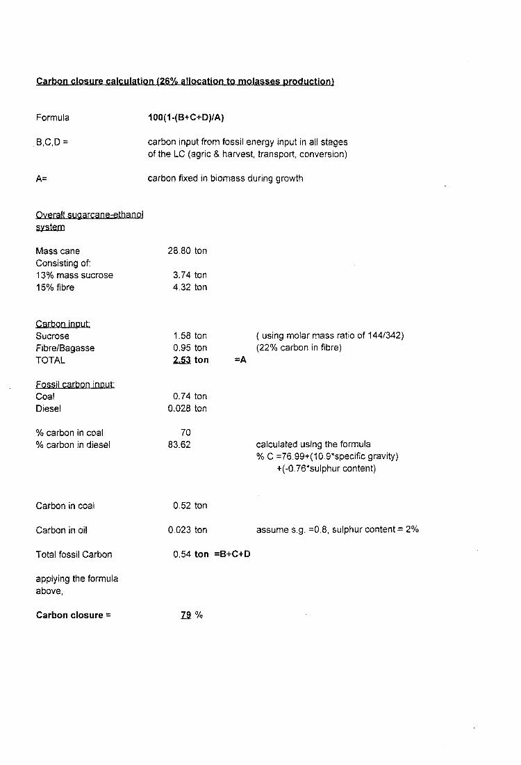
Carbon closure calculation (26% allocation to molasses production)

Formula

B,C,D=

A=

Oyerall sugarcane-ethanol system

Mass cane Consisting of: 13% mass sucrose 15% fibre

Qa[!;2QO ioput; Sucrose Fibre/Bagasse TOTAL

EQ~~il Qa[CQO ioput· Coal Diesel

% carbon in coal % carbon in diesel

Carbon in coal

Carbon in oil

Total fossil Carbon

applying the formula above,

Carbon closure =

100(1-(B+C+O)/A)

carbon input from fossil energy input in all stages of the LC (agric & harvest, transport, conversion)

carbon fixed in biomass during growth

28.80 ton

3.74 ton 4.32 ton

1.58 ton 0.95 ton 2.5.3. ton

0.74 ton 0.028 ton

70 83.62

0.52 ton

0.023 ton

0.54 ton

n%

( using molar mass ratio of 144/342) (22% carbon in fibre)

=A

calculated using the formula % C =76.99+(10.9*specific gravity)

+( -0. 76*sulphur content)

assume s.g. =0.8, sulphur content = 2%

=B+C+O

Calcylation of foss;1 energy ratio

Formula: Energy output (in fuel) I Fotal fossil energy input

Energy in 1 kl ethanol

Calorific values ethanol Coal diesel

Diesel input

MJ/kg MJlkg MJ/kg

30 28 45

overall bioenergy system

24000 MJ

agriculture 30.06 kg sugarcane to molasses process molasses to ethanol process transport TOTAL

Coal input molasses to ethanol process coal

Total Fossil E Input

Fossil energy ratio

0.54 kg 12.82 kg 43.42 kg 1953.9 MJ

0.74 ton 2.Q12.Q MJ

22673.9 MJ/kl

.1Jl6

26% allocation to molasses 7.82 kg

0.54 kg 5 kg

13.3556 kg 601.0 MJ

0.74 ton 2.Q12.Q MJ

21321 MJ/kl

1.13

zero allocation to m . olasses a kg

0.54 kg .5 kg

5.54 kg

0.74 ton

249.3 MJ

2.Q1.2.Q MJ

20969.3 MJ/kl

1.14

Appendix Cl

Primary data for the sugarcane to molasses process

RAW DATA FOR THE SUGARCANE TO MOLASSES PROCESS

Input Process Chemicals Products If, by-products

WEEK --------- .-NO. Cane Water water J cane lime flocculant e_D?jI!!I~ ___ Sugar

tons ratio tons kg kg tons

1 41683 24578 0.59 38 950 30 2420 2 54692 32562 060 29 625 90 3826 3 ~~:~6

26205 0.50 37 1300 60 3842 4

i--------21566 0.47 31 1250 15 3448

5 41767 21847 0.52 30 775 45 3481 6 56485 23349 0,41 39 500 0 4740 7 67744 21407 0.32 47 1000 a .~ 8 49892 20957 0,42 27 525 a 4703 9 65733 29899 OA5 46 600 0 6504

10 67043 33165 0.49 37 275 10 6918 11 67167 27354 041 47 650 0 6967 12 68518 29408 0.43 38 525 15 7344 13 65626 27240 0.42 33 625 60 7255 14 67585 19494 029 33 500 45 7453 15 71932 25002 0.35 35 375 0 8223 16 72694 23009 0.32 35 400 210 8483 17 73146 19823 0.27 37 550 0 8710

----------18 70BOO 19867 0.28 35 450 15 84~ 19 60637 16985 028 30 500 90 7310 20

- ----- 64158 21929 0.34 42 450 75 7991 ---- -

21 70612 1896.0 0.27 35 650 0 8641 22 68654 22100 0.32 42 875 1 8630 23 68826 28085 0.41 49 1025 0 --1m 24 67925 29127 0.43 46 750 0 25 41825 19658 0.47 26 525 75 4830 26 67160 31097 0.46 44 675 2?~ 8314 2: 69620 32194 0.46 4~ 675

~----

105 8655 28 63049 30693 0.49 37 750 165 7637 29 58892 30913 052 29 800

i~o 7181

30 54997 37737 0.69 33 650 --------~€m3

----

31 64359.5 33278 0.52 40 450 30 7457 32 59082 32524 0.55 35 675 225 6803 33 58474 36891 0.63 35 525 21' 6797

1----------- ----------34 50945 29880 0.59 26 700 45 5773 35 60195 24457 0.41 37 1025 360 6997 36 35348 23724 0.67 20 550 120 3874 37 51078 22704 0.44 24 575 480 5342 38 34853 22558 0.65 25 525 90 3512 39 17778 19187 1.08 13 575 180 1714 40 33730 22399 0.86 24 525 390 3529 41 51821 37681 0.73 26 825 120 5444 42 51505 33315 0.65 36 625 380 5399 43 45528 2602: 0.57 23 725 45 4606 44 18682 25133 1.35 12 125 80 1755

----------

TOTAL 2490132 1156188 22 1488 28625 4555 271422 AVERAGE 56594 26277 0.50 33.82 650.57 103.52 616868 MIN 17778 16985 0.27 1200 125.00 0.00 1714.00 MAX 73146 37881 135 49.00 1300.00 48000 8951.00

RAW DATA FOR THE SUGARCANE TO MOLASSES PROCESS (CONTINUED)

Effluent Internal Flows

WEEK Fuel moisture Effluent 21 bar steam NO. Molasses Bagasse Filter cake

----chemical Coal in baClass" cane fIbre eroouced to downslfeam

tons tons tons tons tons % tons m3 ·········toos

1 2069 14453 656 293 3334 52 6997 9088 ~k~~~ 2 .. 3264 17326 469 478 2012 50 8734 5689 3 2591 16356 629 481 18~~ 49 83Se 594 18773 4 1874 13900 546 381 2069

--

49 7157 n~~ 5 1625 12834 501 353 1900 47 6829 9556

6 2070 18293 678 490 1827 49 9275 9219 19536 ___ 7 - 2525 20956 813 577 1563 49 1 (J755 6725 - ----- _._--_ .. _---"-- ~~ ~ .....

8 1650 15032 599 400 1810 47 7955 13851 9 2535 20275 789 5~ 1668 49 10375 16227 2: 182

10 2516 20182 805 596 1638 49 10293 6331 2169, 11 2582 20150 806 581 1596 49 10321 5444 ;m~ 12 2428 19877 822 614 1588 48 10330 12587

13 2469 19023 788 588 1650 48 1~ix1} 10847

----21741

14 2473 19264 811 568 1318 48 16092 .;~~~ _ ..... 15 2548 20753 963 663 1575 47 10904 12664 16 2811 20753 872 608 1519 48 10800 9535 ;;~~; 17 2821 21116 878 652 1567 48 11001 6852 18 2608 21179 850 633 1454 48 10990 9156 23113 19 2369 17832 728 480 1511 48 9253 7690 18171 20 2456 19599 770 553 1453 48 10127 8233 20885 21 2742 21710 847 614 1314 48 11261 7532 22502 22 2696 20875 824 568 1382 49 10680 8137 21212 23 2542 20308 826 620 1343 48

i~~l 8525 22379

24 2654 20248 815 618 1472 48 6129 23228 25 1559 13749 502 302 1316 47 7276 8780 12889 26 2 00 21474 800 584 1094 48 11102 4632 22784 27 2728 21288 835 628 1154 48

ici~~~ c·· .~~~ --~----- 23Q43 28 2257 20337 757 536 ;~~ 48 21026 29 2298 18526 707 513 48 9693 6239 21671 30 1908 17956 660 484 1796 47 9544 6490 ------ 19355 31 2203 21678 773 519 1334 48 ii236 , 6585 19618 32 2092 19865 709 493 1483 48 10347 4682 20940 33 2207 19690 702 506 1396

.. ~~ ... 10268 28217 21652 34 1944 17177 611 430 1188 8803 2895 16034 35 2287. 19876 722 561 1637 48 10375 14188 22918 36 1344 12199 424 331 1479 48 6345 9823 15021 37 1867 16979 613 431 1833 47 8994 8648 16777 38 1448 12115 418 307 1459 48 6357 14307 1~801 39 883 6053 213 122 921 46 3246 12219 4928 40 1171 11572 405 300 1275 48 6073 8403 10279 41 2115 17026 621 489 1728 47 9041 9113 20068 42 1969 17002 618 492 1742 47 8951

17g 20859 43 1940 14759 546 439 1750 48 7705 17619 44 924 6373 224 200 2009 49 3260 1259 10698

TOTAL 96982 777985 29851 21673 69759 403686 370689 842317 AVERAGE 2204.14 17681.48 678.43 492.57 1585 48 9175 8621 19144 MIN 883.00 6053.44 213.00 122.00 921 46.38 3245854528 0 4928 MAX 3284.00 21710.00 87800 663.00 3334 51.59 11260977 28217 23346

RAW DATA FOR THE SUGARCANE TO MOLASSES PROCESS (CONTINUED)

Internal Flows (continued) High Pressure Steam Low Pressure Steam Electricity WEEK LP steam to Boiler 1 Boiler 4 BOiler 2 BOiler 3

NO. mill LP condensate 31 bar steam 31 bar steam 21 bar 21 bar tons tons tons tons tons tons MWh

------1 5451 5426 6225 28105 6979 6536 1299 2 8858 8284 16438 17125 6544 6754 1463 3 9323 7758 14721 16736 6184 6522 ----00 4 7897 5193 10119 17219 6403 6437 ---~ 5 6681 5065 8206 17764 6484 6380 1285 6 9967 7542 14483 18117 -~ 7590 -----~

11750 9417 19174 --------

7 18361 .-~ 7819 __ . ____ 1~ -----8388 6815 15101 17244

----------

8 5250 6122 1333 9 12686 9763 18137 18252 7710 7529 1497 c------

10 12961 9701 20134 18079 6487 7601 1480 11 13351 10048 21067 17555 5603 7567 1469 12 12489 10201 21283 16992 7087 7282 1507 13 12700 9488 19672 17861 6636 7173 1466 14 11922 9339 19547 17014 6734 7003 1421 15 13211 10819 22305 17939 6417 7150 1513 16 13065 11091 22944 18523 7654 4671 1536 17 12764 10734 22711 16844 7364 8095

--~

18 13120 10998 22158 18128 7822 7582 1531 19 10066 8718 13497 18610 6865 7841 1361 20 11676 10469 19109 18505 6735 6828 1501 21 12497 11028 19994 18465 7011 7264 2302 22 11582 10730 20664 18842 5384 7636 1566 23 12785 10614 18648 18701 6781 7361 ---~ 24 13144 10660 19540 19203 7227 7395 1526 25 7069 6129 10016 15440 5495 4827 1122 26 12819 14286 21188 18221 6609 6887 1502

_. 27 12884 12941 21599 18428 5756 7429 --~

28 12005 12121 18307 18623 6849 7206 -----15i7

--29 12544 13017 18245 17142 6688 6105 1490 30 10892 10187 15916 17909 5963 6513 -~ 31 11589 9674 19322 19083 5619 5697 ----~ 32 13068 11707 17942 17168 6626 6667 1502 33 13329 12029 17793 17219 6731 7031 1457 34 9487 10056 14613 15523 5456 5267 1173 ------35 13669 13470 17459 18826 6529 6764 1496 36 8899 7402 7549 14889 5054 5384 1098 37 9689 9603 15103 17861 4465 6129 1310 38 7686 7231 8533 14130 4797 4701 1000 39 2298 2978 1645 10119 2937 3749 --~

40 5051 6296 6658 12179 4473 4481 926 41 11298 9623 17742 17562 4423 6874 1449 42 11953 11338 15297 18265 6527 6892 -J]l! 43 9289 10422 11534 17852 6614 6764 1243 44 4883 5220 3175 11221 5105 5841 851

TOTAL 468755 415631 705513 767844 274723 291346 61213 AVERAGE 10654 9446 16034 17451 6244 6622 1391 MIN 2298 2978 1645 10119 2937 3749 619 MAX 13669 14286 22944 28105 7822 8095 2302

Appendix C2

Prilllary data for the lllolasses to ethanol process

RAW DATA FOR MOLASSES TO ETHANOL PROCESS Utilities and raw

Distillation products material consumption

Month potable industrial absolute feints heads coal power water steam steam kl kl kl kl tons kWh kl tons GJ

Apr-0O 2,914 64 628 60 2,730 681,308 65,065 23,045 65,432 May-0O 2,074 64 501 51 1,858 516,339 49,051 17,569 49,351 Jun-OO 2,098 107 391 51 1,841 535,728 47,087 15,937 44,677 Jul-OO 1,823 107 411 72 2,277 539,015 53,277 15,139 42,051

Aug-0O 2,915 8 598 102 2,422 607,283 53,660 18,604 51,730 Sep-OO 1,776 44 306 52 1,554 390,631 29,203 12,042 33,761 Oct-0O 3,676 85 633 79 2,857 575,988 62,815 19,963 57,026 Nov-OO 3,038 23 561 71 2,407 578,481 58,853 18,546 52,738 • Dec-0O 2,215 90 335 54 2,025 484,717 44,767 14,875 41,863 Jan-01 3,146 18 546 68 2,648 496,571 43,574 18,750 53,292 Feb-01 2,984 114 398 69 2,623 594,525 54,506 19,153 53,601 Mar-01 2,107 37 362 46 1,574 330,972 27,085 12,615 35,023

Average 2,564 63 472 65 2,235 527,630 49,079 17,187 48,379 Minimum 1,776 8 306 46 1,554 330,972 27,085 12,042 33,761 i

Maximum 3,676 114 633 102 ,

2,857 681,308 65,065 23,045 65,432 I

RAW DATA FOR MOLASSES TO ETHANOL PROCESS (2\ . ,

Process chemicals --------- ----~

Month Caustic Soda 47% Caustic Soda 100% Formalin MgS04 CuS04 Urea cyclohexane tons tons tons tons tons tons I

Apr-DO 18.44 12.87 0 1.18 0 6.00 972 May-DO 16.64 11.61 0.004 0.73 0 6.50 1458 Jun-oo 17.85 12.46 0.002 0.40 0 4.50 1458 Jul-oO 5.64 3.94 0 0.58 0 5.50 2430

Aug-DO 20.59 14.37 1.335 0.85 0 7.00 486 ---------

Sep-oo 8.67 6.05 0.45 0.30 0 4.00 967 Oct-DO 17.49 12.21 2.67 0.98 0 11.35 952 Nov-DO 16.28 11.36 1.335 0.80 0 11.70 1428 Dec-DO 17.75 12.39 1.335 0.80 0 8.00 1190

f----

Jan-01 15.21 10.62 1.56 0.43 0 6.00 185 ---------

Feb-01 13.97 9.75 1.11 0.15 0 3.75 740 Mar-01 12.21 8.52 1.335 0.00 0 2.00 800

Average 15 11 1 1 - 6 1089 Minimum 6 4 - - - 2 185 Maximum 21 14 3 1 - 12 2430 ,

RAW DATA FOR MOLASSES TO ETHANOL PROCESS (3)

Gaseous emissions Effluent CO2

Month C02(fossil) (renewable) CO NOx S02 total effluent tons tons tons tons tons kl

Apr-OO 6,745 2,549 32 5 13 60736 May-OO 4,591 2,025 18 3 8 66994

------ --

Jun-OO 4,548 1,800 24 - 9 66384 Jul-OO 5,820 1,933 13 4 7 68942

Aug-OO 6,190 2,567 18 5 17 71288 Sep-OO 3,971 1,479 8 3 14 57589 Oct-OO 7,337 3,443 8 6 20 72839 Nov-OO 6,180 2,735 42 5 24 74844 Dec-OO 5,200 1,936 4 12 66420 Jan-01 6,800 2,680 6 18 59516

-----------

Feb-01 6,736 2,413 6 18 64815 Mar-01 4,043 1,859 2 8 47835

Average 5,680 2,285 21 5 14 64850 Minimum 3,971 1,479 8 2 7 47835 Maximum 7,337 3,443 42 6 24 74844