A Layout Algorithm for Undirected

Compound Graphs ?

Ugur Dogrusoz a,b,∗ Erhan Giral b Ahmet Cetintas a Ali Civril c

Emek Demir d

aComputer Engineering Dept., Bilkent University, Ankara, Turkey

bTom Sawyer Software, Oakland, CA, USA

cRensselaer Polytechnic Institute, Troy, NY, USA

dMemorial Sloan-Kettering Cancer Center, New York, NY, USA

Abstract

We present an algorithm for the layout of undirected compound graphs, relaxing re-

strictions of previously known algorithms in regards to topology and geometry. The

algorithm is based on the traditional force-directed layout scheme with extensions to

handle multi-level nesting, edges between nodes of arbitrary nesting levels, varying

node sizes, and other possible application-specific constraints. Experimental results

show that the execution time and quality of the produced drawings with respect

to commonly accepted layout criteria are quite satisfactory. The algorithm has also

been successfully implemented as part of a pathway integration and analysis toolkit

named PATIKA, for drawing complicated biological pathways with compartmental

constraints and arbitrary nesting relations to represent molecular complexes and

various types of pathway abstractions.

Key words: Information visualization, graph drawing, force-directed graph layout,

compound graphs, bioinformatics

Preprint submitted to Elsevier 5 November 2008

1 Introduction

As graphical user interfaces have improved, and more state-of-the-art soft-

ware tools have incorporated visual functions, interactive graph editing and

diagramming facilities have become important components in visualization

systems [7]. Effective analysis of the underlying data in graph visualization is

only possible with the sound automatic layout capabilities of such systems.

The notion of compound graphs has been used, in the past, to represent more

complex types of relationships or varying levels of abstractions in data (see

Figures 1 and 2) [20,17,16,14].

Fig. 1. Part of a sample compound pathway.

? A short demo version of this paper appeared in Proc. of 12th Intl. Symposium

on Graph Drawing, NYC, New York, pp. 442-447, Sept. 29 – Oct. 2, 2004.∗ Address: Computer Engineering Dept., Bilkent University, Ankara 06800, Turkey,

Tel: +90 (312) 290 1612, Fax: +90 (312) 266 4047.Email address: ugur@cs.bilkent.edu.tr (Ugur Dogrusoz).

2

There has been a great deal of work done on general graph layout [4] but con-

siderably less on the layout of compound graphs, probably due to the difficult

nature of the problem. Straightforward approaches to laying out compound

graphs in a top-down or bottom-up manner (with respect to the inclusion

or nesting hierarchy) fail, due to bidirectional dependencies (e.g., inter-graph

edges) between levels of varying depth. The limited work on compound graph

layout has mostly focused on the layout of hierarchical graphs [19,18,9], in

which the underlying relational information is assumed to be under a certain

hierarchy. However, such algorithms perform poorly if the graph is undirected

(if the edge directions do not enforce a hierarchy) but still has structural prop-

erties, like symmetry, or includes parts or substructures, such as cycles. The

work on undirected compound graphs [1,21,12,10,3,5], on the other hand, is

either restricted in the types of graphs addressed (e.g., clustered graphs, where

grouping or nesting is allowed for only one level) or is unsatisfactory in terms

of the quality of results produced (e.g., large compound nodes overlapping

with others or an inefficient use of area).

In this paper, we describe a new algorithm for the layout of undirected com-

pound graphs that overcomes the shortcomings of previous algorithms. Ours is

based on the force-directed layout algorithm [8,13] and is the first for drawing

undirected compound graphs, to handle all of the following (Figure 3) with a

rather simple, intuitive, force-directed model:

• an arbitrary level of nesting,

• inter-graph edges that may span multiple levels of nesting, and

• links to non-leaf nodes in the nesting hierarchy.

Furthermore, it can handle non-uniform node sizes.

3

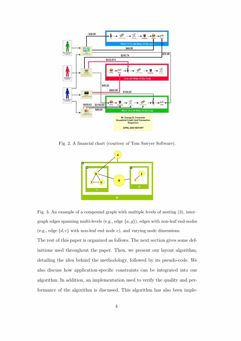
Fig. 2. A financial chart (courtesy of Tom Sawyer Software).

Fig. 3. An example of a compound graph with multiple levels of nesting (3), inter–

graph edges spanning multi-levels (e.g., edge {a, g}), edges with non-leaf end-nodes

(e.g., edge {d, e} with non-leaf end node e), and varying node dimensions.

The rest of this paper is organized as follows. The next section gives some def-

initions used throughout the paper. Then, we present our layout algorithm,

detailing the idea behind the methodology, followed by its pseudo-code. We

also discuss how application-specific constraints can be integrated into our

algorithm. In addition, an implementation used to verify the quality and per-

formance of the algorithm is discussed. This algorithm has also been imple-

4

mented within the software tool Patika [6] to visualize complicated biological

pathways with compartmental constraints and nested drawings. We conclude

with a brief summary.

2 Definitions

We assume the reader is familiar with basic notation and definitions of graph

theory. A node v ∈ V (an edge e ∈ E), where G = (V,E), is said to be a

member of graph G; conversely, G is said to be the owner of node v (edge

e). A compound graph C = (V,E, F ) consists of nodes V , adjacency edges E,

and inclusion edges F . It is required that the inclusion graph T = (V, F ) is a

rooted tree, and no adjacency edge connects a node to one of its descendants

or ancestors. For instance, for the compound graph in Figure 3,

V = {a, b, · · · , j},

E = {{a, b}, {a, g}, {d, e}, {d, g}, {f, g}, {f, h}, {g, h}, {i, j}}, and

F = {bc, bd, be, cf, cg, ch, ei, ej}.

For convenience, our implementation represents unrestricted undirected com-

pound graphs with geometry information using a graph manager. A graph

manager M = (S, I, F ) defined by a graph set S = {G1, G2, . . . , Gl}, an

inter-graph edge set I, and a rooted nesting tree F =(V F , EF

). With this

representation, the topology of a compound graph is split into multiple graphs

that are nested within each other. The geometry of each node is represented

by a rectangle. The nesting of a graph in a node facilitates the drawing of

multiple graphs of a graph manager and their interrelations simultaneously.

The node within which a graph is nested, is said to be expanded. The size of

an expanded node is as big as the boundaries of the associated nested graph.

5

This is represented in the nesting tree by an edge {u,Gi} ∈ EF between a

node u and a graph Gi, where Gi is not a (direct or indirect) owner of u. Gi is

said to be the child graph of the parent node u. The graph at the root of the

nesting tree is simply called root graph.

Another way of associating two different graphs in a graph manager M =

(S, I, F ) is via the inter-graph edge set I. Let u ∈ V Gi and v ∈ V Gj be two

nodes, where i 6= j and Gi, Gj ∈ S. Then, the edge {u, v} ∈ I is called an

inter-graph edge, representing a relation between nodes that belong to different

entities, graphs Gi and Gj in this case.

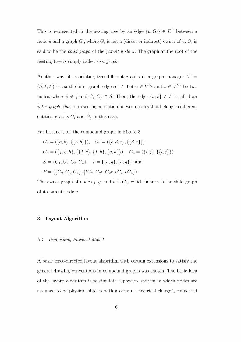
For instance, for the compound graph in Figure 3,

G1 = ({a, b}, {{a, b}}), G2 = ({c, d, e}, {{d, e}}),

G3 = ({f, g, h}, {{f, g}, {f, h}, {g, h}}), G4 = ({i, j}, {{i, j}})

S = {G1, G2, G3, G4}, I = {{a, g}, {d, g}}, and

F = ({G2, G3, G4}, {bG2, G2c,G2e, cG3, eG4}).

The owner graph of nodes f, g, and h is G3, which in turn is the child graph

of its parent node c.

3 Layout Algorithm

3.1 Underlying Physical Model

A basic force-directed layout algorithm with certain extensions to satisfy the

general drawing conventions in compound graphs was chosen. The basic idea

of the layout algorithm is to simulate a physical system in which nodes are

assumed to be physical objects with a certain “electrical charge”, connected

6

via “springs” of a pre-specified desired length. Objects pull or repel each other

depending on the current lengths of any connected springs. In addition, rela-

tively minor repulsion forces act on any pair of objects that are “too close” to

each other to avoid node-to-node overlaps. Furthermore, we assume “gravita-

tional forces” to keep graph components together. In order to handle varying

node sizes (especially expanded nodes) and to avoid overlaps with neighboring

nodes, calculation of edge lengths are based on the parts of edges in between

the borders of end-nodes, as opposed to their centers [15]. Thus, the optimal

layout is regarded as the state of this system, in which the total energy is

minimal. The following additions are made to this basic model:

• An expanded node and its associated nested graph are represented as a sin-

gle entity, similar to a “cart”, which can move freely in orthogonal directions

(no rotations allowed). Multiple levels of nesting is modeled with smaller

carts on top of larger ones (Figure 4).

• The nodes and edges of a nested graph are to be set in motion on this

cart, confined within the bounds of the cart. Each cart is assumed to be

of a special material, elastic enough to adapt to the current bounds of

the associated nested graph. Thus, as nodes of a nested graph are pushed

outwards, expanding the nested graph, the parent node adjusts its bounds

accordingly. Similarly, should the bounds of the nested graph shrink, so will

the geometry of the parent node by the same amount.

• Each nested graph, including the root graph, is assumed to have a dynamic

(with respect to its graph bounds) center of gravity, pulling all its nodes

in, towards its center, so as to keep them together, disallowing arbitrary

drifts from the center. The strength of this force is independent from the

size of the node and the distance between node center and graph center.

7

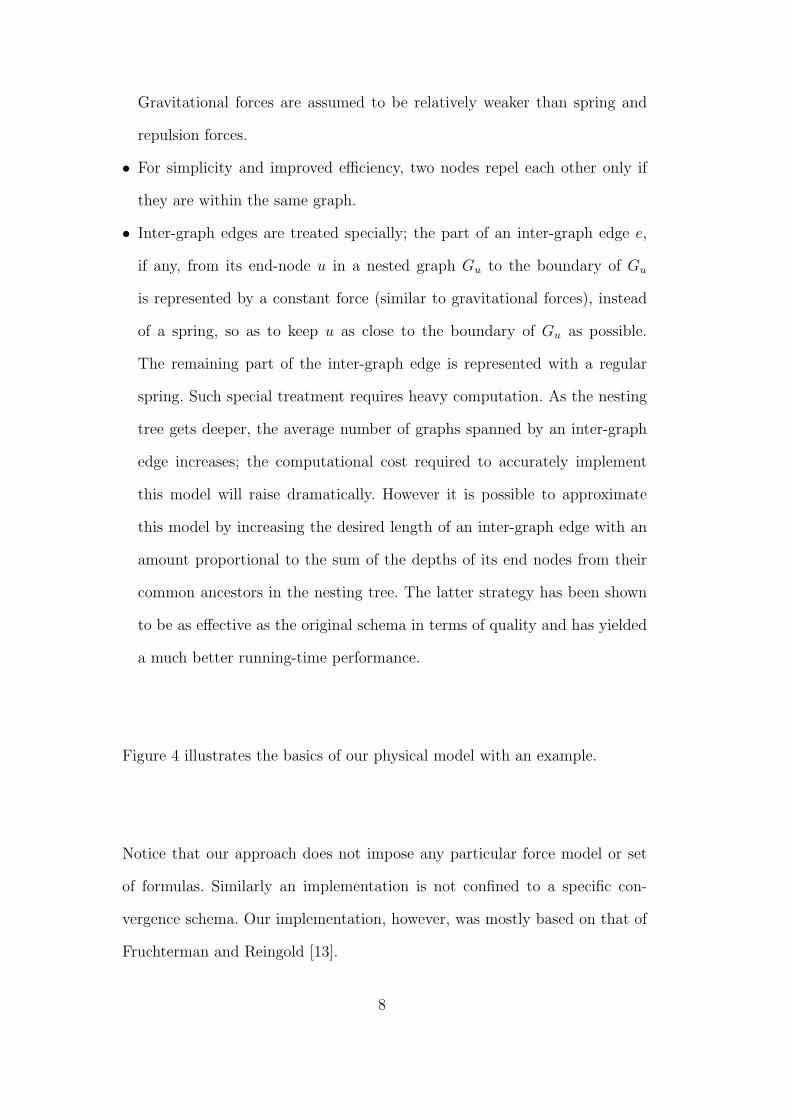
Gravitational forces are assumed to be relatively weaker than spring and

repulsion forces.

• For simplicity and improved efficiency, two nodes repel each other only if

they are within the same graph.

• Inter-graph edges are treated specially; the part of an inter-graph edge e,

if any, from its end-node u in a nested graph Gu to the boundary of Gu

is represented by a constant force (similar to gravitational forces), instead

of a spring, so as to keep u as close to the boundary of Gu as possible.

The remaining part of the inter-graph edge is represented with a regular

spring. Such special treatment requires heavy computation. As the nesting

tree gets deeper, the average number of graphs spanned by an inter-graph

edge increases; the computational cost required to accurately implement

this model will raise dramatically. However it is possible to approximate

this model by increasing the desired length of an inter-graph edge with an

amount proportional to the sum of the depths of its end nodes from their

common ancestors in the nesting tree. The latter strategy has been shown

to be as effective as the original schema in terms of quality and has yielded

a much better running-time performance.

Figure 4 illustrates the basics of our physical model with an example.

Notice that our approach does not impose any particular force model or set

of formulas. Similarly an implementation is not confined to a specific con-

vergence schema. Our implementation, however, was mostly based on that of

Fruchterman and Reingold [13].

8

Fig. 4. Part of a sample compound graph (left) and the corresponding physical

model used by our algorithm, where the deeper a node is in the nesting hierarchy

the lighter it is colored (right).

3.2 Application-Specific Constraints

Today’s sophisticated graph visualization applications require specific con-

straints to be integrated into layout algorithms. These constraints may vary

arbitrarily, however common examples include keeping the relative position

of a group of nodes fixed and clustering a set of nodes that share a common

property worth displaying [2]. However, such constraints generally introduce

conflicting goals, even with the core target of the basic spring embedder itself

(minimal node-node overlap and revealing symmetries).

We propose introducing additional forces to “blend” application-specific con-

straints into our method of drawing undirected compound graphs. In order to

preserve the nice properties of the core spring embedder, in case of conflict, the

default forces should govern such additional forces. Thus, application-specific

forces are set to have constants of relatively smaller factors.

9

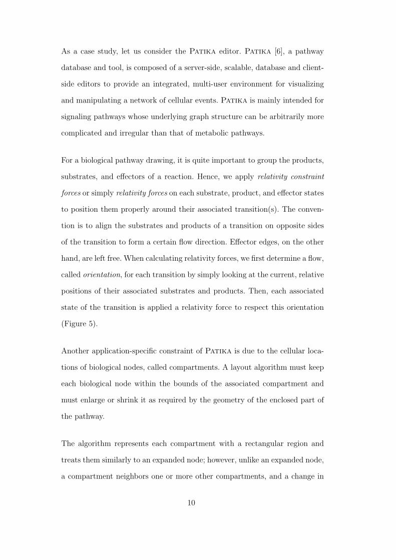
As a case study, let us consider the Patika editor. Patika [6], a pathway

database and tool, is composed of a server-side, scalable, database and client-

side editors to provide an integrated, multi-user environment for visualizing

and manipulating a network of cellular events. Patika is mainly intended for

signaling pathways whose underlying graph structure can be arbitrarily more

complicated and irregular than that of metabolic pathways.

For a biological pathway drawing, it is quite important to group the products,

substrates, and effectors of a reaction. Hence, we apply relativity constraint

forces or simply relativity forces on each substrate, product, and effector states

to position them properly around their associated transition(s). The conven-

tion is to align the substrates and products of a transition on opposite sides

of the transition to form a certain flow direction. Effector edges, on the other

hand, are left free. When calculating relativity forces, we first determine a flow,

called orientation, for each transition by simply looking at the current, relative

positions of their associated substrates and products. Then, each associated

state of the transition is applied a relativity force to respect this orientation

(Figure 5).

Another application-specific constraint of Patika is due to the cellular loca-

tions of biological nodes, called compartments. A layout algorithm must keep

each biological node within the bounds of the associated compartment and

must enlarge or shrink it as required by the geometry of the enclosed part of

the pathway.

The algorithm represents each compartment with a rectangular region and

treats them similarly to an expanded node; however, unlike an expanded node,

a compartment neighbors one or more other compartments, and a change in

10

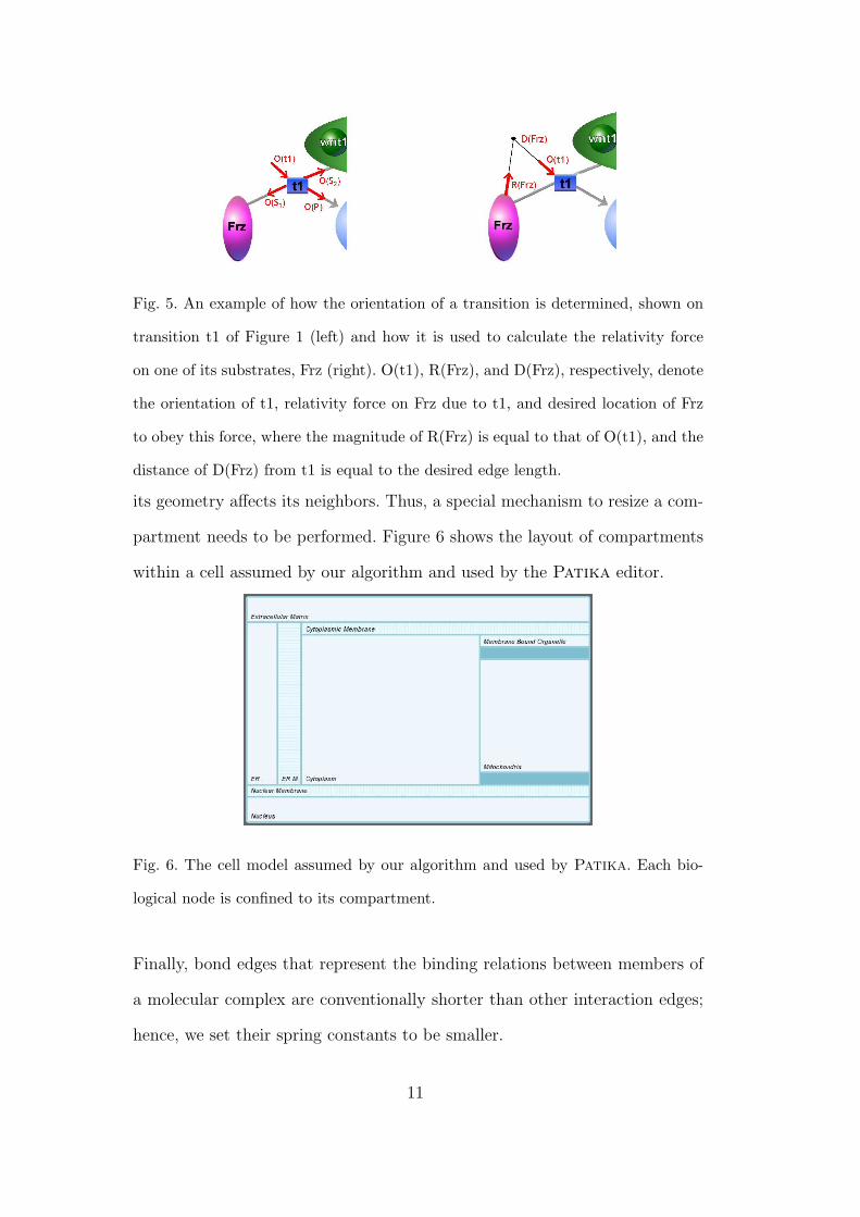
Fig. 5. An example of how the orientation of a transition is determined, shown on

transition t1 of Figure 1 (left) and how it is used to calculate the relativity force

on one of its substrates, Frz (right). O(t1), R(Frz), and D(Frz), respectively, denote

the orientation of t1, relativity force on Frz due to t1, and desired location of Frz

to obey this force, where the magnitude of R(Frz) is equal to that of O(t1), and the

distance of D(Frz) from t1 is equal to the desired edge length.

its geometry affects its neighbors. Thus, a special mechanism to resize a com-

partment needs to be performed. Figure 6 shows the layout of compartments

within a cell assumed by our algorithm and used by the Patika editor.

Fig. 6. The cell model assumed by our algorithm and used by Patika. Each bio-

logical node is confined to its compartment.

Finally, bond edges that represent the binding relations between members of

a molecular complex are conventionally shorter than other interaction edges;

hence, we set their spring constants to be smaller.

11

Figure 18 shows a sample biological pathway drawing produced by the layout

algorithm, as implemented within the Patika editor.

3.3 Algorithm

We assume that the graph to be laid out is represented with a graph manager

object M = (S, I, F ), where each graph G = (V,E) in S is implemented using

an adjacency list representation, and V M and EM , respectively, represent all

nodes (both simple and compound) and edges (both intra and inter-graph) in

graph manager M . These objects can be referenced through structures named

GraphMgr, Graph, Node, and Edge. Layout specific data and functionality are

assumed to be kept in these structures as well.

The algorithm is composed of three major phases preceded by an initialization

phase:

• Initialization: This is where initial node sizes, and threshold values for

determining convergence (based on number of nodes) are calculated, and

the random initial positioning of nodes is performed.

In addition, for efficiency and layout quality reasons, parts of the given

graph that are trees are temporarily removed. In other words, a root graph’s

leaf nodes are iteratively removed until no such node is left. The remaining

part of the graph forms the “skeleton” of the graph (see Figure 7).

The overall time complexity of this method is Θ(|V M |), as each node is

visited Θ(1) times.

12

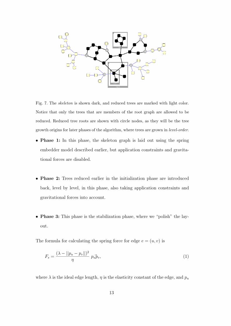
Fig. 7. The skeleton is shown dark, and reduced trees are marked with light color.

Notice that only the trees that are members of the root graph are allowed to be

reduced. Reduced tree roots are shown with circle nodes, as they will be the tree

growth origins for later phases of the algorithm, where trees are grown in level-order.

• Phase 1: In this phase, the skeleton graph is laid out using the spring

embedder model described earlier, but application constraints and gravita-

tional forces are disabled.

• Phase 2: Trees reduced earlier in the initialization phase are introduced

back, level by level, in this phase, also taking application constraints and

gravitational forces into account.

• Phase 3: This phase is the stabilization phase, where we “polish” the lay-

out.

The formula for calculating the spring force for edge e = (u, v) is

Fs =(λ− ||pu − pv||)2

η~pupv, (1)

where λ is the ideal edge length, η is the elasticity constant of the edge, and pu

13

and pv are positions of nodes u and v, respectively. The ideal edge length of an

inter-graph edge is increased proportional to the sum of the depths of its end

nodes from their common ancestors in the nesting tree. Non-uniform node

dimensions require force calculations to be based on clipping points rather

than node centers. The following method is used for calculating the spring

forces acting on each edge’s ends:

algorithm CalculateSpringForces(GraphMgr M)

1) for e = (u, v) ∈ EM do

2) idealLength := λ

3) if e is an inter-graph edge then

4) idealLength ∗= (u.depth+ v.depth)∗NESTING FACTOR

5) cu := LineSegment(u.center, v.center) ∩ u.boundRect

6) cv := LineSegment(u.center, v.center) ∩ v.boundRect

7) Fs := (idealLength− ||cu − cv||)2/η · ~cucv

8) Fs(u) += Fs

9) Fs(v) −= Fs

The overall time complexity of this method is Θ(|EM |), as all steps inside the

for-loop can be processed in Θ(1) steps.

Node-to-node repulsion forces are calculated using the formula

Fr =α

||pu − pv||2~pupv, (2)

where α is the repulsion constant. Similar to spring forces, repulsion forces

require us to make clipping point calculations for nodes of non-uniform size,

based on the lines passing through nodes’ centers:

14

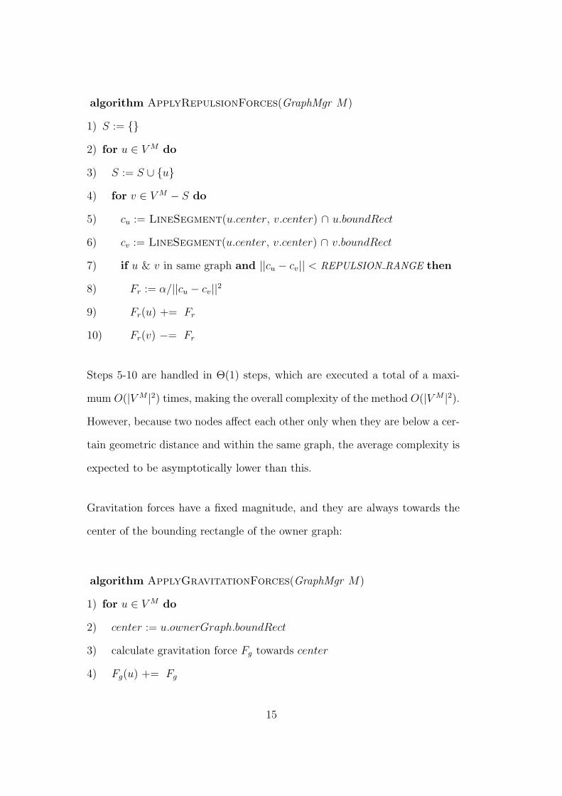
algorithm ApplyRepulsionForces(GraphMgr M)

1) S := {}

2) for u ∈ V M do

3) S := S ∪ {u}

4) for v ∈ V M − S do

5) cu := LineSegment(u.center, v.center) ∩ u.boundRect

6) cv := LineSegment(u.center, v.center) ∩ v.boundRect

7) if u & v in same graph and ||cu − cv|| < REPULSION RANGE then

8) Fr := α/||cu − cv||2

9) Fr(u) += Fr

10) Fr(v) −= Fr

Steps 5-10 are handled in Θ(1) steps, which are executed a total of a maxi-

mum O(|V M |2) times, making the overall complexity of the method O(|V M |2).

However, because two nodes affect each other only when they are below a cer-

tain geometric distance and within the same graph, the average complexity is

expected to be asymptotically lower than this.

Gravitation forces have a fixed magnitude, and they are always towards the

center of the bounding rectangle of the owner graph:

algorithm ApplyGravitationForces(GraphMgr M)

1) for u ∈ V M do

2) center := u.ownerGraph.boundRect

3) calculate gravitation force Fg towards center

4) Fg(u) += Fg

15

The overall time complexity of this method is Θ(|V M |), as all steps inside the

for-loop can be processed in Θ(1) time.

Fig. 8. Sample compound graphs (with varying desired edge lengths and edge and

inter-graph edge density) laid out by our algorithm. The nodes are color-coded to

denote the depth of the node in the nesting hierarchy (i.e., the deeper a node is, the

darker its color is).

16

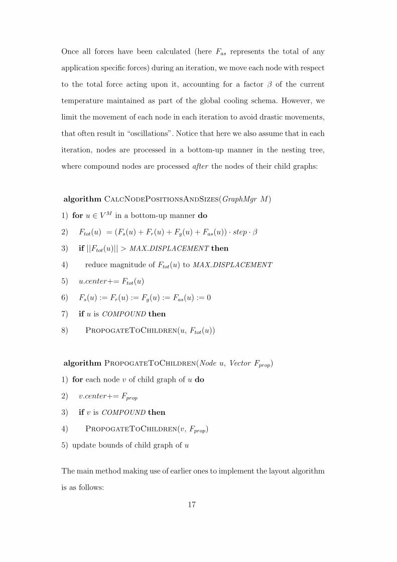
Once all forces have been calculated (here Fas represents the total of any

application specific forces) during an iteration, we move each node with respect

to the total force acting upon it, accounting for a factor β of the current

temperature maintained as part of the global cooling schema. However, we

limit the movement of each node in each iteration to avoid drastic movements,

that often result in “oscillations”. Notice that here we also assume that in each

iteration, nodes are processed in a bottom-up manner in the nesting tree,

where compound nodes are processed after the nodes of their child graphs:

algorithm CalcNodePositionsAndSizes(GraphMgr M)

1) for u ∈ V M in a bottom-up manner do

2) Ftot(u) = (Fs(u) + Fr(u) + Fg(u) + Fas(u)) · step · β

3) if ||Ftot(u)|| > MAX DISPLACEMENT then

4) reduce magnitude of Ftot(u) to MAX DISPLACEMENT

5) u.center+= Ftot(u)

6) Fs(u) := Fr(u) := Fg(u) := Fas(u) := 0

7) if u is COMPOUND then

8) PropogateToChildren(u, Ftot(u))

algorithm PropogateToChildren(Node u, Vector Fprop)

1) for each node v of child graph of u do

2) v.center+= Fprop

3) if v is COMPOUND then

4) PropogateToChildren(v, Fprop)

5) update bounds of child graph of u

The main method making use of earlier ones to implement the layout algorithm

is as follows:

17

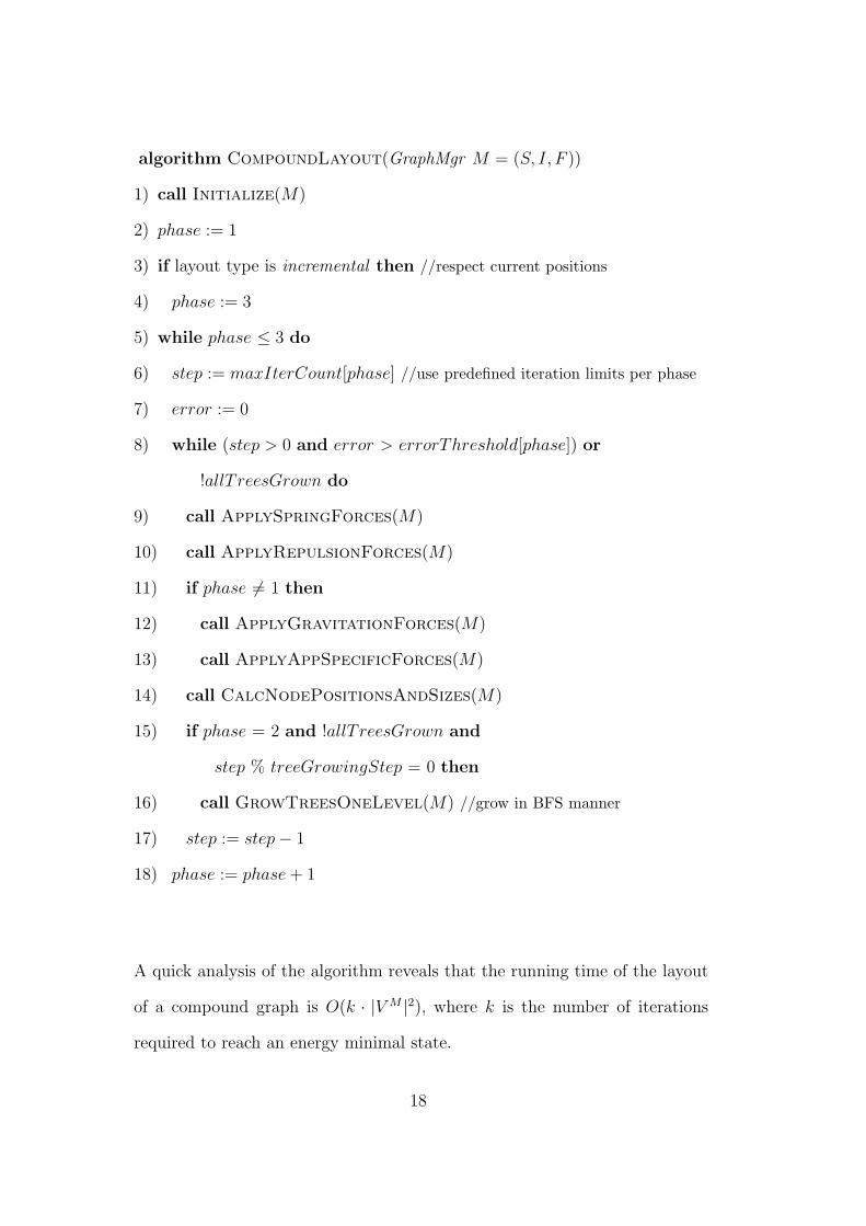
algorithm CompoundLayout(GraphMgr M = (S, I, F ))

1) call Initialize(M)

2) phase := 1

3) if layout type is incremental then //respect current positions

4) phase := 3

5) while phase ≤ 3 do

6) step := maxIterCount[phase] //use predefined iteration limits per phase

7) error := 0

8) while (step > 0 and error > errorThreshold[phase]) or

!allT reesGrown do

9) call ApplySpringForces(M)

10) call ApplyRepulsionForces(M)

11) if phase 6= 1 then

12) call ApplyGravitationForces(M)

13) call ApplyAppSpecificForces(M)

14) call CalcNodePositionsAndSizes(M)

15) if phase = 2 and !allT reesGrown and

step % treeGrowingStep = 0 then

16) call GrowTreesOneLevel(M) //grow in BFS manner

17) step := step− 1

18) phase := phase+ 1

A quick analysis of the algorithm reveals that the running time of the layout

of a compound graph is O(k · |V M |2), where k is the number of iterations

required to reach an energy minimal state.

18

4 Implementation

The algorithm described above has been tested within the example appli-

cation of Tom Sawyer Visualization for Java, version 7.0. The development

environment was Sun’s Java SDK 1.4 and Microsoft Windows XP operating

system on an ordinary personal computer (Pentium IV with 2GHz CPU and

512MB memory). The results were found quite satisfactory, as far as the gen-

eral graph drawing criteria, such as number of crossings, and total area are

concerned (Figures 8 and 9). Furthermore, the experimental executions were

found to be not only reasonably fast for interactive use but also in line with

the earlier theoretical analysis, as detailed below.

4.1 Experimental Results

We performed experiments on the execution time of our layout algorithm on

randomly generated graphs with one of several parameters changing for each

set. For each test, a random graph manager to be laid out was generated with

the provided parameters:

• n: total number of nodes,

• m/n: proportion of number of edges to nodes; the number of edges is as-

sumed to be linear in the number of nodes,

• mig/m: proportion of inter-graph edges to number of all edges,

• d: maximum nesting depth,

• b: maximum branching (i.e., number of children of a node) in the nesting

tree,

• p: probability of pruning a child in the nesting tree to avoid nesting trees

19

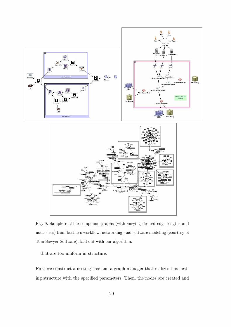
Fig. 9. Sample real-life compound graphs (with varying desired edge lengths and

node sizes) from business workflow, networking, and software modeling (courtesy of

Tom Sawyer Software), laid out with our algorithm.

that are too uniform in structure.

First we construct a nesting tree and a graph manager that realizes this nest-

ing structure with the specified parameters. Then, the nodes are created and

20

distributed to graphs in the graph manager uniformly. Similarly, end nodes

of each edge are picked randomly. Each test is executed 10 times, and the

average is taken. For simplicity, we take the dimensions of leaf nodes to be

uniform, even though our algorithm is able to handle non-uniform dimensions

for not only non-leaf (compound) nodes but also leaf nodes. Figure 10 shows

an example of a randomly generated graph.

Fig. 10. A randomly generated graph laid out by our algorithm.

(n = 70, m/n = 1.5, mig/m = 0.03, d = 3, b = 3, and p = 0.33)

Fig. 11. Number of nodes (n) vs. execution time of our algorithm.

(m/n = 1.5, mig/m = 0.05, d = 3, b = 3, and p = 0.33)

21

From the theoretical analysis given earlier, a quadratic behavior of execution

time is expected, assuming k does not grow in the order of the graph size. The

experiments validate this argument (Figure 11).

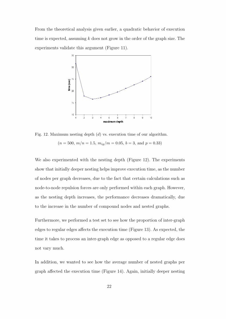
Fig. 12. Maximum nesting depth (d) vs. execution time of our algorithm.

(n = 500, m/n = 1.5, mig/m = 0.05, b = 3, and p = 0.33)

We also experimented with the nesting depth (Figure 12). The experiments

show that initially deeper nesting helps improve execution time, as the number

of nodes per graph decreases, due to the fact that certain calculations such as

node-to-node repulsion forces are only performed within each graph. However,

as the nesting depth increases, the performance decreases dramatically, due

to the increase in the number of compound nodes and nested graphs.

Furthermore, we performed a test set to see how the proportion of inter-graph

edges to regular edges affects the execution time (Figure 13). As expected, the

time it takes to process an inter-graph edge as opposed to a regular edge does

not vary much.

In addition, we wanted to see how the average number of nested graphs per

graph affected the execution time (Figure 14). Again, initially deeper nesting

22

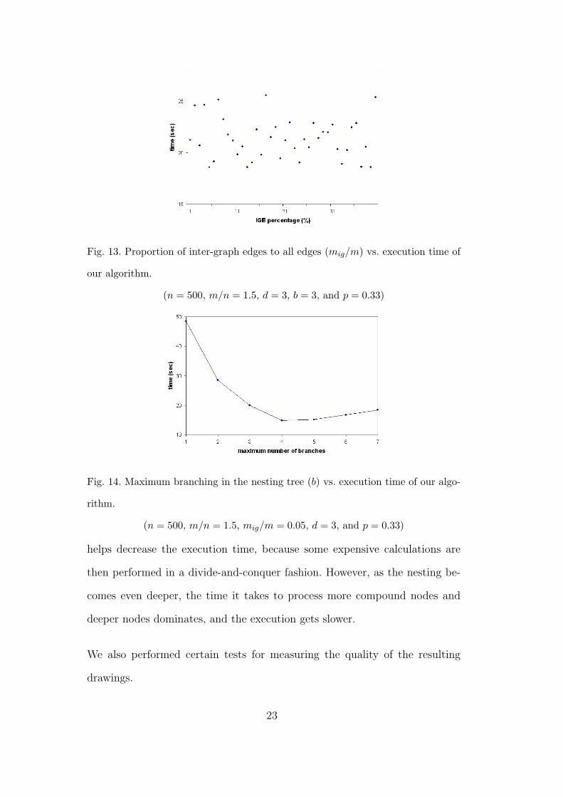
Fig. 13. Proportion of inter-graph edges to all edges (mig/m) vs. execution time of

our algorithm.

(n = 500, m/n = 1.5, d = 3, b = 3, and p = 0.33)

Fig. 14. Maximum branching in the nesting tree (b) vs. execution time of our algo-

rithm.

(n = 500, m/n = 1.5, mig/m = 0.05, d = 3, and p = 0.33)

helps decrease the execution time, because some expensive calculations are

then performed in a divide-and-conquer fashion. However, as the nesting be-

comes even deeper, the time it takes to process more compound nodes and

deeper nodes dominates, and the execution gets slower.

We also performed certain tests for measuring the quality of the resulting

drawings.

23

The first set of quality tests were performed to check for node-to-node overlaps.

It is extremely hard to completely eliminate node overlaps for drawings of non-

uniform node dimensions that are generated by a spring embedder, due to

the fact that the constants associated with opposing attraction and repulsion

forces are difficult to fine-tune. The results yielded node-to-node overlaps of

only, at most, one node pair in a thousand, and the overlap amounts are almost

always inconsequential.

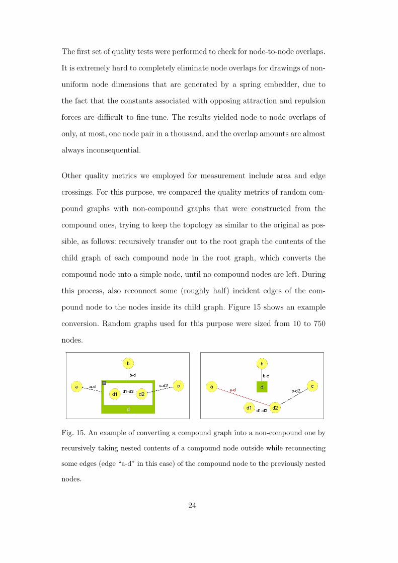
Other quality metrics we employed for measurement include area and edge

crossings. For this purpose, we compared the quality metrics of random com-

pound graphs with non-compound graphs that were constructed from the

compound ones, trying to keep the topology as similar to the original as pos-

sible, as follows: recursively transfer out to the root graph the contents of the

child graph of each compound node in the root graph, which converts the

compound node into a simple node, until no compound nodes are left. During

this process, also reconnect some (roughly half) incident edges of the com-

pound node to the nodes inside its child graph. Figure 15 shows an example

conversion. Random graphs used for this purpose were sized from 10 to 750

nodes.

Fig. 15. An example of converting a compound graph into a non-compound one by

recursively taking nested contents of a compound node outside while reconnecting

some edges (edge “a-d” in this case) of the compound node to the previously nested

nodes.

24

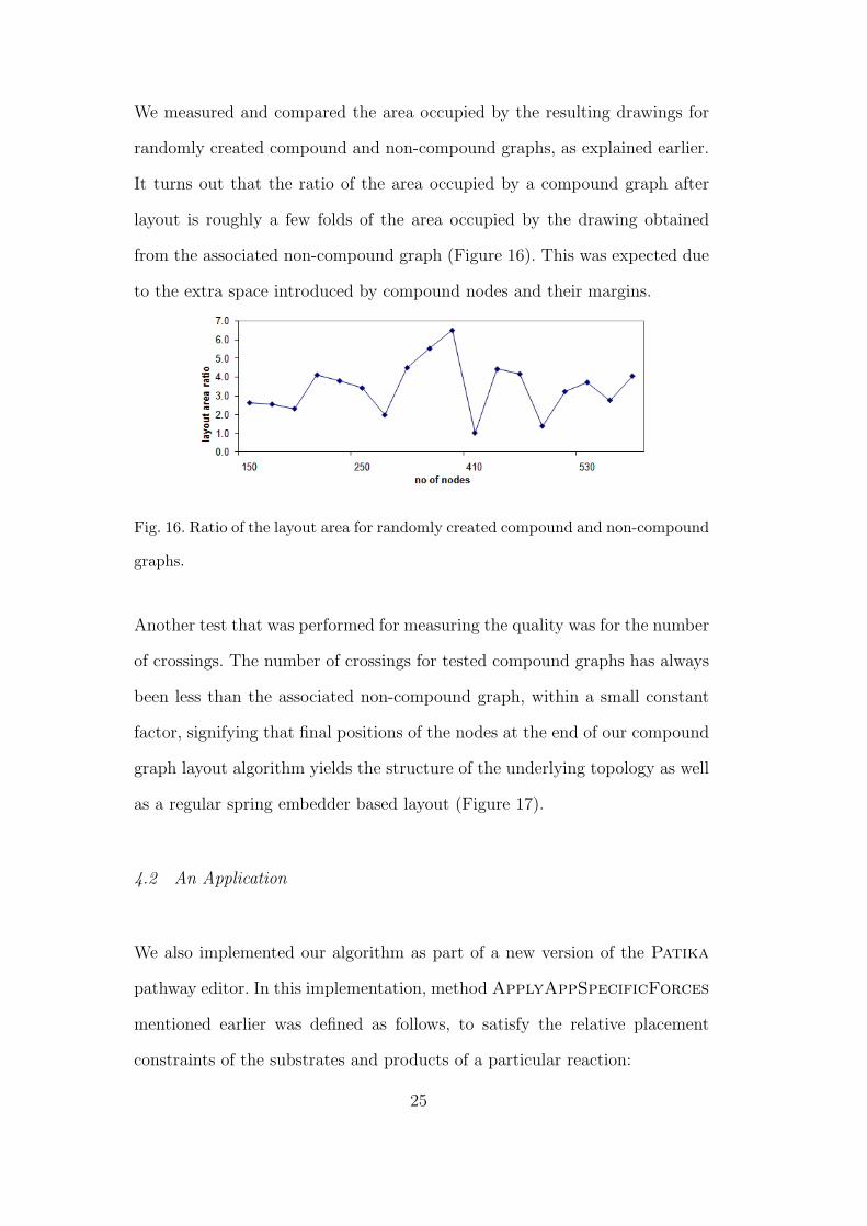
We measured and compared the area occupied by the resulting drawings for

randomly created compound and non-compound graphs, as explained earlier.

It turns out that the ratio of the area occupied by a compound graph after

layout is roughly a few folds of the area occupied by the drawing obtained

from the associated non-compound graph (Figure 16). This was expected due

to the extra space introduced by compound nodes and their margins.

Fig. 16. Ratio of the layout area for randomly created compound and non-compound

graphs.

Another test that was performed for measuring the quality was for the number

of crossings. The number of crossings for tested compound graphs has always

been less than the associated non-compound graph, within a small constant

factor, signifying that final positions of the nodes at the end of our compound

graph layout algorithm yields the structure of the underlying topology as well

as a regular spring embedder based layout (Figure 17).

4.2 An Application

We also implemented our algorithm as part of a new version of the Patika

pathway editor. In this implementation, method ApplyAppSpecificForces

mentioned earlier was defined as follows, to satisfy the relative placement

constraints of the substrates and products of a particular reaction:

25

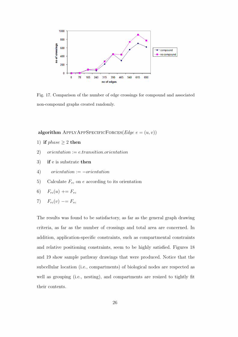
Fig. 17. Comparison of the number of edge crossings for compound and associated

non-compound graphs created randomly.

algorithm ApplyAppSpecificForces(Edge e = (u, v))

1) if phase ≥ 2 then

2) orientation := e.transition.orientation

3) if e is substrate then

4) orientation := −orientation

5) Calculate Frc on e according to its orientation

6) Frc(u) += Frc

7) Frc(v) −= Frc

The results was found to be satisfactory, as far as the general graph drawing

criteria, as far as the number of crossings and total area are concerned. In

addition, application-specific constraints, such as compartmental constraints

and relative positioning constraints, seem to be highly satisfied. Figures 18

and 19 show sample pathway drawings that were produced. Notice that the

subcellular location (i.e., compartments) of biological nodes are respected as

well as grouping (i.e., nesting), and compartments are resized to tightly fit

their contents.

26

Fig. 18. A sample pathway (obtained by a query from the Patika database) laid

out by our algorithm.

4.3 Implementation Issues

The use of “momentum” or “temperature” for each node [11] has helped the

convergence greatly. Each node’s movement is not only based on the total

force calculated during the current iteration but also on the previous one. For

simplicity and efficiency reasons, we simply added a constant portion of the

previous iteration’s total force to this iteration’s total force for each node,

27

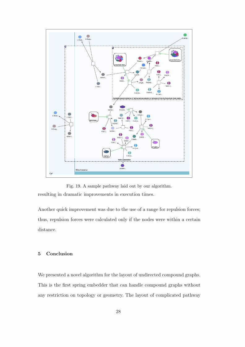
Fig. 19. A sample pathway laid out by our algorithm.

resulting in dramatic improvements in execution times.

Another quick improvement was due to the use of a range for repulsion forces;

thus, repulsion forces were calculated only if the nodes were within a certain

distance.

5 Conclusion

We presented a novel algorithm for the layout of undirected compound graphs.

This is the first spring embedder that can handle compound graphs without

any restriction on topology or geometry. The layout of complicated pathway

28

graphs, such as those in Patika, are among the target applications. The main

novelties of our work include the use of a modified spring embedder system that

treats compound nodes and inter-graph edges as part of the physical system. In

addition, we believe that most application-specific drawing conventions, such

as those in biological pathways, can be integrated into this physical system as

additional forces, as long as they can be sketched out as part of the physical

model described. Experimental results are found satisfactory both in terms of

the quality of layouts and computational efficiency.

References

[1] F. Bertault, M. Miller, An algorithm for drawing compound graphs, in: Graph

Drawing (Proc. GD ’99), vol. 1731 of Lecture Notes in Computer Science,

Springer-Verlag, (1999) 197–204.

[2] K. Bohringer, F. Paulisch, Using constraints to achieve stability in automatic

graph layout algorithms, in: CHI ’90 Proceedings, ACM, (1990) 43-51.

[3] G. Di Battista, W. Didimo, A. Marcandalli, Planarization of clustered graphs,

in: Graph Drawing (Proc. GD ’01), vol. 2265 of Lecture Notes in Computer

Science, Springer-Verlag, (2001) 60-74.

[4] G. Di Battista, P. Eades, R. Tamassia, I. G. Tollis, Graph Drawing, Algorithms

for the Visualization of Graphs, Prentice-Hall, 1999.

[5] E. Di Giacomo, W. Didimo, L. Grilli, G. Liotta, Graph visualization techniques

for web clustering engines, IEEE Transactions on Visualization and Computer

Graphics 13 (2) (2007) 294–304.

[6] U. Dogrusoz, E. Erson, E. Giral, E. Demir, O. Babur, A. Cetintas, R. Colak,

PATIKAweb: a Web interface for analyzing biological pathways through

29

advanced querying and visualization, Bioinformatics 22 (3) (2006) 374–375.

[7] U. Dogrusoz, Q. Feng, B. Madden, M. Doorley, A. Frick, Graph visualization

toolkits, IEEE Computer Graphics and Applications 22 (1) (2002) 30–37.

[8] P. Eades, A heuristic for graph drawing, Congressus Numerantium 42 (1984)

149–160.

[9] P. Eades, Q. Feng, X. Lin, Straight-line drawing algorithms for hierarchical

graphs and clustered graphs, in: S. North (ed.), GD ’96, vol. 1190 of Lecture

Notes in Computer Science, Springer-Verlag, (1997) 113–128.

[10] P. Eades, M. Huang, Navigating clustered graphs using force-directed methods,

Journal of Graph Algorithms and Applications 4 (3) (2000) 157–181.

[11] A. Frick, A. Ludwig, H. Mehldau, A fast adaptive layout algorithm for

undirected graphs, in: R. Tamassia, I. Tollis (eds.), GD ’94, vol. 894 of Lecture

Notes in Computer Science, Springer-Verlag, (1995) 388-403.

[12] Y. Frishman, A. Tal, Dynamic drawing of clustered graphs, in: Proceedings of

IEEE Symposium on Information Visualization, (2004) 191-198.

[13] T. M. J. Fruchterman, E. M. Reingold, Graph drawing by force-directed

placement, Software Practice and Experience 21 (11) (1991) 1129–1164.

[14] K. Fukuda, T. Takagi, Knowledge representation of signal transduction

pathways, Bioinformatics 17 (9) (2001) 829–837.

[15] D. Harel, Y. Koren, Drawing graphs with non-uniform vertices, in: Working

Conference on Advanced Visual Interfaces (Proc. AVI’02), ACM Press, (2002)

157-166.

[16] W. Lai, P. Eades, A graph model which supports flexible layout functions, Tech.

Rep. 96-15, Callaghan 2308, Australia (1996).

30

[17] M. Raitner, HGV: A library for hierarchies, graphs, and views, in: M. Goodrich,

S. Kobourov (eds.), Proc. Graph Drawing ’02, vol. 1528 of LNCS, (2002) 236–

243.

[18] G. Sander, Layout of compound directed graphs, Tech. Rep. A/03/96,

University of Saarlandes, CS Dept., Saarbrucken, Germany (1996).

[19] K. Sugiyama, K. Misue, Visualization of structural information: Automatic

drawing of compound digraphs, IEEE Transactions on Systems, Man and

Cybernetics 21 (4) (1991) 876–892.

[20] K. Sugiyama, K. Misue, A generic compound graph visualizer/manipulator: D-

ABDUCTOR, in: F. J. Brandenburg (ed.), GD ’95, vol. 1027 of Lecture Notes

in Computer Science, Springer-Verlag, (1995) 500-503.

[21] X. Wang, I. Miyamoto, Generating customized layouts, in: F. Brandenburg

(ed.), Graph Drawing (Proc. GD ’95), vol. 1027 of Lecture Notes in Computer

Science, Springer-Verlag, (1995) 504-515.

31