ELSEVIER

An Intemational Joumal Available online at www.sciencedirect.corn computers &

.c,-.c.~o,.-cT. mathematics with applications

Computers and Mathematics with Applications 51 (2006) 1647-1662 www.elsevier.com/locate/camwa

A Hybrid G M R E S / L S - A r n o l d i Method to Accelerate the Parallel Solution

of Linear Systems

HAIWU HE, C . BERGERE AND S. P E T I T O N Laboratoire d ' Informatique Fondamentale de Lille

Universit~ des Sciences et Technologies de Lille 59655 Villeneuve D'Ascq, France

<he><bergereg><pet it on>~lif i. fr

A b s t r a c t - - W e present a parallel hybrid asynchronous method to solve large sparse linear systems by the use of a large parallel machine. This method combines a parallel GMRES(m) algorithm with the least squares method that needs some eigenvalues obtained from a parallel Arnoldi algorithm. All of the algorithms run on different processors of an IBM SP3 or IBM SP4 computer simultaneously. This implementation of this hybrid method allows us to take advantage of the parallelism available and to accelerate the convergence by decreasing considerably the number of iterations. (~) 2006 Elsevier Ltd. All rights reserved.

K e y w o r d s - - L i n e a r algebra, Sparse matrices, Iterative method, GMRES, Hybrid method, Arnoldi, Least squares, Parallelism.

1. I N T R O D U C T I O N

Many scientific applications require the resolution of linear systems of the form

A x = b,

where A is an n x n real matrix, b is a real vector, and x is the real vector of the solution of the system. Such systems are often implanted by large sparse matrices; this sparse structure is very helpful to solve a large linear system.

The computation and storage of GMRES(m) [1] allows us to resolve such linear systems with a very large scale. In addition, it allows computing sparse matrices in a compressed format, without loading zeros in memory, because it preserves the sparse structure. I t has been implemented on a parallel machine [2], but this method cannot always converge very fast. There are some ways to accelerate the convergence of GMRES. One of these is to calculate in parallel some eigenvalues by the Arnoldi method [3,4]. As soon as they are approximated with sufficient accuracy, eigenvalues are used to perform some iterations of the least squares method [5] for getting a better initial vector for the next GMRES restart.

In this paper, we first present in Section 2 the numerical methods used in our hybrid method. We propose a parallel algorithm for the hybrid method and we study the implementation on

0898-1221/06/$ - see front matter (~) 2006 Elsevier Ltd. All rights reserved. Typeset by .A.h~-2"~X doi:10.1016/j.camwa.2006.05.004

1648 H. HE et al.

the supercomputer IBM SP3 (of USTL 1) and IBM SP4 (of CINES 2) (in Section 3). Important parameters and numerical results are discussed for this implementation (in Section 4), and the advantages of this method are shown by numerical examples.

2. T H E G M R E S ( M ) / L S - A R N O L D I (K,L) H Y B R I D P A R A L L E L M E T H O D

2.1. Arno ld i P r o c e s s

The Arnoldi process gives an orthonormai basis Vm = Iv1, v2 , . . . , vm] of the Krylov subspace

KIn(A, v) = span (v, A v , . . . , A m - i v ) ,

where A E 9~ "xn, and v E 9I n.

There is one variant of the algorithm which results from a recursive application of the Gram- Schmidt (GS) process on the columns of the matrix [vl, A v l , . . . , Avm-1], where Vl is the nor- malized vector v.

ALGORITHM 1: ARNOLDI PROCESS.

1. Compute ~ = Ilvl12, and v~ = v / ~ . 2. For j = 1 , . . . , m do

hi,j = (Avj ,v i ) , :for i = l , . . . , j w Av3 J = - ~ i=l h~,jvi, compute hj+l,j ---- HwlI2, and Vj+l = w/hj+l,j

end do

H,~ is the (m + 1) x m upper Hessenberg matrix whose nonzero entries are the coefficients hi,/. Therefore, we obtain this important relation

AVm = Vm+t[Im. (2.1)

Let Hm be the m × m upper Hessenberg matrix obtained from Hm by removing its last row, then we can write

H,~ = V~ AVm, (2.2)

and (2.1) can be rewritten

AVm = VmHm + hm+l,mVm+lerm, (2.3)

where em is the m TM canonical vector of 9l m. The Gram-Schmidt method we use above is the classical Gram-Schmidt process (CGS). The

modified Gram-Schmidt process (MGS) is another variant of the GS process; in addition it is more stable than CGS. But we cannot parailelize it so well. We can remedy the stability drawback of CGS by reorthogonalizing the vector V3+l at every iteration or only if a loss of orthogonality is detected. The method adopted by Kelley in [6] is based on the Brown/Hindmarch condition; the reorthogonalization is done if

I1Avjl[2 + ~llwl12 = IIAvjlh

in working precision, with 6 ---- 10 -3. The Arnoldi process will be used in the GMRES solver, and in Arnoldi's method for computing

eigenvalues and eigenvectors of large sparse matrices, to perform the projection onto the Krylov

subspace KIn(A, v). For the parallel implementation of the Arnoldi process, in the previous methods, we will use the reorthogonalized CGS version, because it is both parallelizable and stable.

~USTL: Universit~ des Sciences et Technologies de Lille, Lille, France. 2CINES: Centre Informatique National de l'Enseignement Sup~rieur, Montpellier, France.

A Hybrid CMRES/LS-Arnoldi Method 1649

2.2. G M R E S M e t h o d

In 1986, Saad and Schultz described the GMRES (generalized minimum residual) method, see [1] as a Krylov subspace method for solving nonsymmetric systems. The m TM (m ~ 1) iterate x,~ of GMRES is the solution of the least squares problem

min lib - A x l ] 2 , (2.4) Z6xo+km (A,ro)

where ro = b - A x o is the residual of the initial solution. The Arnoldi process applied to K m ( A , ro) builds Vm+l = [Vm, Vm+l] and /~m which satisfy

formula (2.1).

Since K I n ( A , to) = span(v, A v , . . . , A ' ~ - l v ) , the iterate Xm has the following form:

X m ~- XO + Vmym,

where Ym ~ [Rm, and its residual r m can be presented as follows:

b - A x m = b - A ( x o + V,~ym)

-- ro - A V m Y m

= y m + l - Bmy ),

where el is the first canonical vector of 9~ m+l. Now we can compute the norm of rm, and we have

H,-,,,H2 = I]v,,,+l 1[2

Therefore, ym is the solution of the following least squares problem:

min 11/3el-/-Imyll 2 . (2.5)

A powerful tool for solving this optimization problem is the QR decomposition based on House- holder transformations [7].

The major drawback to GMRES is that the amount of work and storage required per iteration rises linearly with the iteration count. Unless one is fortunate enough to obtain extremely fast convergence, the cost will rapidly become prohibitive. The usual way to overcome this limitation is by restarting the iteration. After a chosen number of iterations m, the accumulated data are cleared and the intermediate results are used as the initial data for the next m iterations. This procedure is repeated until convergence is achieved. The difficulty is in choosing an appropriate value for m. If m is too small, GMRES(m) may be slow to converge, or fail to converge entirely. A value of m that is larger than necessary involves excessive work (and uses more storage). Unfortunately, there are no definite rules governing the choice of m, and choosing when to restart is a matter of experience. Some helpful preconditioned GMRES methods [8] are also studied for a better convergence.

The GMRES(m) algorithm uses the traditional GMRES algorithm iteratively, by finding the iterate Xm, and restarting the algorithm with the initial guess x0 = xm, until convergence. Thus, we obtain the restarted GMRES(m) after m iterations of GMRES.

ALGORITHM 2: GMRES(m) . i. Start: choose xo an initial guess of the solution, m the dimension of Krylov

subspaces, and g the tolerance,

compute ro = b - Axo.

1650 H. HE et al.

100

80

r

8 60

i,= 40

20

, . . . P-T ime GMRE:S i tself (n,,,JT00.m,,358)

- IBM SP3 ~ I E ~ A SP4

\ \

, , , , , , , ,

2 3 4 5 6 7 8 9 10 11 12 N u m b e r o f P r o c e s s o r s

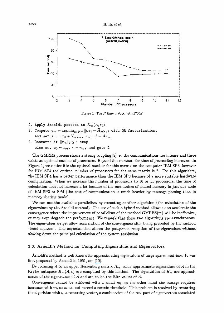
Figure 1. The P-time matrix "utmlT00a'.

2. Apply Arnoldi process to Km(A, ro). 3. Compute Ym-'-argminue~ libel- [Imy]12 with QR factorization,

and se t X m = 370 Jr YrnYTr~, rm ---- b - A x m .

4. R e s t a r t : i f Ilrmll~ < ~ s t o p

else set xo ----- Xm, r ---~ r m , and goto 2

The GMRES process shows a strong coupling [9], so the communications are intense and there exists an optimal number of processors. Beyond this number, the time of proceeding increases. In Figure 1, we notice 9 is the optimal number for this matrix on the computer IBM SP3, however for IBM SP4 the optimal number of processors for the same matrix is 7. For this algorithm, the IBM SP4 has a better performance than the IBM SP3 because of a more suitable hardware configuration. When we increase the number of processors to 10 or 11 processors, the time of calculation does not increase a lot because of the mechanism of shared memory in just one node of IBM SP3 or SP4 (the cost of communication is much heavier by message passing than in memory sharing mode).

We can use the available parallelism by executing another algorithm (the calculation of the eigenvalues by the Arnoldi method). The use of such a hybrid method allows us to accelerate the convergence where the improvement of parallelism of the method GMRES(m) will be ineffective, or may even degrade the performance. We remark that these two algorithms are asynchronous. The eigenvalues we get allow acceleration of the convergence after being preceded by the method "least squares". The asynchronism allows the postponed reception of the eigenvalues without slowing down the principal calculation of the system resolution.

2.3. A r n o l d i ' s M e t h o d for C o m p u t i n g E igenva lues a n d E i g e n v e c t o r s

Arnoldi's method is well known for approximating eigenvalues of large sparse matrices. It was first proposed by Arnoldi in 1951, see [10].

By reducing A to an upper Hessenberg matrix Hm, some approximate eigenva/ues of A in the Krylov subspace K m ( A , v ) are computed by this method. The eigenvalues of Hm are approxi- mates of the eigenvalues of A and are called the Ritz values of A.

Convergence cannot be achieved with a small m; on the other hand the storage required increases with m, so m cannot exceed a certain threshold. This problem is resolved by restarting the algorithm with v, a restarting vector, a combination of the real part of eigenvectors associated

A Hybrid GMRES/LS-Arnoldi Method 1651

with the d desired dominant eigenvalues. We can choose v in the form

d

v = E R e ( u , ) i= l

Thus, Arnoldi's method for computing d dominant eigenvalues and their associated eigenvectors is as follows.

ALGORITHM 3: ARNOLDI"S METHOD. 1. S t a r t : choose v an i n i t i a l vec to r , m the dimension of g ry lov subspaces,

and d the number of des i r ed dominant e igenva lues , with the t h r e s h o l d 6. 2. Apply the Arnoldi p rocess to K , , ( A , v ) .

3. Compute the e igenvalues (hi, 1 < i < d) and the a s s o c i a t e d e igenvec to r s

(yi, l < i < d ) of Hr, . 4. Set u i = V m y i , f o r i = l , . . . , d , the Ri tz v e c t o r s

5. Compute Pi = [[Aiui - Aui]]2, i = 1 , . . . , d .

6. R e s t a r t : i f maxd=l [Pi] < z s top d e l se se t v = ~ i = l R e ( u i ) , and goto 2.

After convergence in order to find another eigenvalue, we can deflate the matrix or choose a starting vector v orthogonal to the eigenvectors associated with the eigenvalues already computed, see [11-13].

2.4. Leas t Squares M e t h o d

Just like all Krylov subspace methods, the iterates of the least squares method can be written as follows:

5c = xo + P k ( A ) r o , (2.6)

where x0 is an initial approximation, r0 its initial residual, and Pk is a polynomial of degree k - 1. Let p~ be the subset of the real polynomials space defined by

p~ = {polynomials p of degree k, such that p(0) = 1},

and define the polynomial Rk E p~ by R k ( z ) = 1 -- z P k ( z ) . Then the residual of the iterate ~ is

= R k ( A ) r o .

Suppose that A is diagonalizable. Denote by {ul, u2,.. . ,u,~} its eigenvector basis, and a ( A ) =

{A1,--., A~} its spectrum. If we express r0 in the eigenvector basis as

n

r0 ----- E pilQ' i=l

then we can rewrite ~ in this way

= ~ piRk()~i)ui . i=l

An overestimate of the Euclidean norm of ~ is given by

11~ll2 ~ Itr0112 m~)IRk(~)l .

It is natural to choose Rk so that the above bound of []7=]]2 is minimal; in this case Rk is the solution of the following min max problem:

min max IRk(A)I. (2.7) Rk6P~ AEa(A)

1652 H. HE et al.

Since we do not have the whole spectrum of A, but only some eigenvalue estimates contained in a convex hull H, we consider the problem

min max IRk(A)I. (2.8) RkEP~ XEH

It is known that maxx~H ]Rk()~)l is reached on the polygonal boundary OH of H, and thus (2.8) becomes

min max ]Rk()~)l. (2.9) RkEP~ )~EOH

The above min max problem is difficult to solve. To address this difficulty, Smolarski and Say- tor [14] proposed to change the uniform norm (i.e., maxwell IRk()QI) by weighted L2-norm on the space of real polynomials, with a suitable weight function w. We obtain the following minimiza- tion problem:

min [IRkll~,. (2.10) RkEP~

Let OH + be the upper part of OH, and denote by Ev (v = 1 , . . . ,#) its edges, and hence we have E 0H+ = U.=I v. Let c. and d, be, respectively, the centre and the half width of the edge Ev.

The inner product (., .)~ over the space of real polynomials, associated with the norm II-Hw, is defined after simplification by

where w~, is the restriction of w on the edge E, w~ is defined by

~ . ( ~ ) = 2 id ~ _ (~ _ c~ )=t -~ /= . (2.12) 71"

This weight is the generalized weight on a complex edge associated with the Chebyshev basis T~(()~-c,)/d,) . This property makes the computation of the inner product easier by expressing p and q in this basis on each edge E , as follows:

z p ( ~ ) = V " F! ' )T. . ~ - c~ ~ ~ - z_., ~ ~ , q(;~) = {~')Ti , (2.13) i = 0 i = 0

then we have

= 2 R o + , 2 1 4 ,

Let (tj)j > 0 be the scaled and shifted Chebyshev basis

((~ - c ) / d ) tj()~) = Tj Tj(a/d) ' j = 0 , 1 , . . . . (2.15)

This is the best basis of polynomials on the ellipse ¢(c, d, a) of smallest area enclosing H (see [15] and [16] for an algorithm computing this optimal ellipse). Moreover it satisfies a three-term recurrence of the form

~ + l t i + l ( z ) = ( z - ~ , ) t , ( z ) - ~ t , _ l ( Z ) , i = o, 1 , . . . . ( 2 . 1 8 )

Using the (tj)j > 0 basis defined by (2.15) we obtain a well-conditioned modified Gram matrix Mk = (mi,j) defined by

mi,j = ( tz- l , t j -1)w, i , j C { 1 , . . . , k + 1}. (2.17)

We can express Pk in the Chebyshev basis as follows: k--1

Pk = ~ ~iti, i = 0

where the coefficients ~i are determined by a minimization problem similar to problem (2.5) seen in CMRES with a Hessenberg matrix obtained from Mk and the coefficients ai, ~i, 5i. For more details, see [3].

A Hybrid GMRES/LS-Arnoldi Method 1653

2.5. T h e H y b r i d A l g o r i t h m GMRES(m) /LS(k , 1)

This algorithm includes two parts. In the first part we use the GMRES(m) method to solve the linear system. In the second part, we find some eigenvalue estimates, and we apply the least squares method iteratively l times and we restart the GMRES(m) algorithm.

The algorithm can be given as follows.

ALGORITHM 4: GMRES(m)LS(k , I ) .

i. Start: Choose xo, m, m' the dimension of Krylov subspaces, k the degree of

the least squares polynomial, 6 the threshold and I the number of successive

application of the least squares method.

2. Compute Xm, the m th iterate of GMRES starting with xo, if

llb-Axml]2 <6 Stop else set xo =Xm, ro=b-Axo.

3. Perform simultaneously m' iterations of Arnoldi process on the other

processors starting with to, and compute the eigenvalues of Sm,.

4. If the number of eigenvalues obtained is sufficient then compute the least

squares polynomial Pk on the boundary of H the convex hull enclosing all

computed eigenvalues.

5. For j= l,...,l do

Compute ~ ---- x0 + Pk(A)ro, and set Xo ---- x, ro = b- Axo.

End do

6. Restart: if lit0(12 < 6 stop else goto 2.

Suppose that the computed convex hull H contains only the eigenvalues AI,..., As, so the last

residual is given by

s

= (Rk(A)/ro = ~ p (Rk(Ai/) u~ + p (Rk(Ai) l) ui. i=1 i=s+l

The first part of the residual is very small because the LS method finds Rk minimizing IRk(A)[ with A E H, but not the second part, so the residual will be rich in the eigenvectors associated to the eigenvalues outside the convex hull H.

We can tell that as l increases the first part will be much closer to zero and the second part will be very large. This explains the fact that residual norm increases enormously. However, restarting GMRES(m) with an iterate of which the residual norm is enormous.

Restarting GMRES(m) with an iterate of which the residual is a combination of a small number of eigenvectors, the convergence will be very fast even if the residual norm is enormous.

Because of the reason above, it is better to take the LS residual as the initial vector of Arnoldi's method in order to find new eigenvalues outside the hull convex H. This technique is used in the least squares Arnoldi method, see [15].

In order to implement this hybrid method, we use the supercomputer "IBM SP3 and SP4". A group of processors is in charge of the GMRES(m) algorithm, and another group takes charge of the parallel Arnoldi algorithm which calculates independently the eigenvalues necessary for the hybridization of the GMRES(m) method. The Arnoldi method includes some parts which can be parallelized (Arnoldi's projection, residuals calculation, restarts). I t is realized by the scientific software parallel package "PARPACK" [17] which runs on a group of processors, and a sequential part (the LS method and the sorting of eigenvalues) which runs on only one processor.

In the Arnoldi method, when the number of eigenvalues whose residual is under the chosen threshold is sufficient, these eigenvalues will be sent to the processors devoted to the sequential part of hybridization. This computation is sequential because it uses just a small set of data; a parallel distribution of them is unnecessary. This process will calculate "least squares" pa- rameters, i.e., parameters of a convex polygon containing the eigenvalues in the complex plan,

1654 H. HE et al.

l

Figure 2. The representation of eigenvalues in the complex plan of a real matrix, the convex, and the ellipse including them.

parameters of the ellipse of smallest area enclosing this convex polygon, and coefficients of the least squares polynomial (see Figure 2).

These parameters are then sent in order to execute the parallel part of the hybridization. The processes executing the GMRES(m) algorithm receive these data in an asynchronous manner, at the end of the current iteration. The GMRES algorithm is then stopped, and the parallel part of the hybridization is realized, by the least squares method, before restarting GMRES with the obtained iterate. The residual of this vector is also sent to the processors which run the Arnoldi's algorithm in order to use it as a new better initial vector for Arnoldi's method.

3. I M P L E M E N T A T I O N

3.1. G e n e r a l O r g a n i z a t i o n

To have experiments on such a system, we choose the supercomputer system IBM SP3 and IBM SP4. For IBM SP3: one SMP architecture with five nodes interconnected by a high debit network. For the four original nodes, each node has 16 processors of 375 MHz and 16 GB memory. For the fifth node updated recently, it has 16 processors of 1.1 GHz and 16 GB memory. For IBM SP4: one SMP architecture with nine nodes Power4 interconnected by a high debit network Federation, each node has 32 processors of 1.3 GHz and 64 GB memory. For our experiments, by reason of

efficiency, and decreasing the communication of network, we execute our programs just on one node of the supercomputer.

Most of the processors are used to run the algorithm GMRES(m) by the way of SPMD (single program multiple data) model, with an administrative process and p identical calculation pro- cesses. The calculation processors read directly their own data and execute the corresponding part of the method GMRES(m), communicating with their sibling processes.

The processors dedicated to the parallel package "PARPACK" [17] contain the reception of residuals, the projection of Arnoldi, and the calculation of eigenvalues. Only one processor calculates the parameters "least squares" (the vertexes of convex polygon, the parameters of

ellipse (a, c, d), and coefficients of the polynomial "least squares" ~i), which will be sent to the processors executing the algorithm GMRES(m) later.

3.2. M a t r i x F o r m a t for t h e I m p l e m e n t a t i o n

Matrices downloaded from the MatrixMarket site are tested for our algorithm. A series of ma- trices used in nuclear physic and computational fluid dynamics are tested: the matrix "utm300"

A Hybrid GMRES/LS-Arnoldi Method 1655

(size 300 × 300, 3155 nonzero elements), 3 the matrix "utmlT00a" (size 1700 × 1700, 21313 nonzero elements), 4 the matrix "utm3060" (size 3060 x 3060, 42211 nonzero elements), ~ and the largest matrix tested "af23560" (size 23560 × 23560, 484256 nonzero elements). 6 In fact, we convert all these matrices into the CSR format for our calculation.

The format most economical in the memory for the machines is the format CSR (compress sparse row) or its equivalence CSC by columns (compress sparse column). The CSR format describes the sparse matrices by three vectors [18,19].

3 . 3 . Eigenvalues A c c u m u l a t i o n

It is necessary to accumulate eigenvalues found during several iterations. Indeed the number of usable eigenvalues (whose residual norms are under the expected accuracy) obtained after each Arnoldi's iteration is not always sufficient to perform another LS iteration. In addition, for a given initial vector, eigenvalues whose accuracy is sufficient are not always the same from one iteration to another.

Moreover, we cannot obtain all the matrix eigenvalues with the Arnoldi method. To obtain a good distribution of the computed eigenvalues, we must use different initial vectors. Each restart of the method is hence established by changing this vector, especially with the residual vector received from GMRES, if it is available. In this way, a satisfactory sampling of eigenvalues is computed that allows us to calculate efficient LS parameters. We therefore save eigenvalues that are found at each iteration. All these values are used to update the LS parameters. Some will be duplicated but these copies do not modify the convex polygon characteristics.

: Amoldi

I lrutiali~tion I

H I I

elgenva/~ s and clgenval,a:s vector~

l /g~nmnb~r o[ ~

,( comp~dc,ge~l=s > "~Ls enousi~ 7 /

\ / "o 2 ..q -

I /'-°°'°°' \ t Take ,* as an mi~*al ~'~ vet.lot ~lac take

~ ~rb~ra~ vector / [

r

/ ('JMP.ES:Lq "~

I"

I '"--' II

. . . .

~t~htd~

1 I

, L . .

. " . . "

Figure 3. The influence of the size of the Krylov subspace in GMRES method MG for "af23560" on IBM SP4.

3See details about this matrix at http ://math. nist. gov/MatrixMarket/data/SPARSKIT/~okamak/ utm300, html. 4See details about this matrix at http://math, nist. gov/MatrixMarket/data/SPARSKIT/tokamak/ utm1700a, html. SSee details about this matrix at http://math, nist. gov/MatrixMarket/data/SPARSKIT/tokamak/ utm3060, html. 6See details about this matrix at http://math.nist, gov/MatrixMarket/data/NEP/airfoil/ af23560, html.

1656 H. HE et al.

3.4 . M e t h o d P a r a m e t e r s

The hybrid algorithm's behaviour is subordinate to many parameters. We describe here the most important of them.

n is the matrix size. m is the size of Krylov's subspace. This parameter exists in both the CMRES method and in

the Arnoldi method. When m decreases, the duration of each iteration decreases, because the amount of calculation becomes smaller. But at the same time, the number of iterations before convergence increases [1]. An optimal value exists that is not necessarily the same in the two algorithms. In addition, we can use these values to adjust the relative speed between the two computations in order to adjust the number of eigenvalues sendings (see Figures 3-6). Thus we shall distinguish between m(GMRES) and m(Arnoldi).

k is the degree of the least squares polynomial. l is the power of the LS computation. It represents the number of times that the LS parameters

will be used at each LS iteration. N V is the minimum number of eigenvalues to accumulate before the calculation of LS param-

eters; it has also a remarkable influence on the performance (see Figure 7). The importance of both k and I is discussed in Section 4 (see Figures 8, 9 and Tables 1, 2).

E =o m

1,0E+02 1,0E+01 1.0E+OO 1,0E-01 1,0E-O2

1,0E-03 1,0E-04 1,0E-05 1,0E-06 1,0E-07 1,0E-08 1,0E-09 1,0E-IO 1,0E-11

1,0E- 12

1,0E-13

1,0E-14 m ~ , , ,

40 60 80 Time(seconds)

HybrldlzaUon with L= 1,5,core~w/ed to GMP.E8 Itself , (n= 1TO0.m(GtMRES)m400,m(Amotdl)=256,k= 15) k

,\ - - GMRES Itself . . . . . L1 - - L 5

\

0 20 100 120 140

Figure 4. The influence of the size of the Krylov subspace in the GMRES method MG for "af23560" on IBM SP4.

1,00E+02

1,00E+01

1,00E+O0

1,00E-01

1,00E-02 1,00E-03

1,00E-04 1,00E-05

1.00E-06 1,00E-07

1,00E-08

1,00E-09

1,00E-10

1.00E-11 1.00E-12

1,00E-13

Hybridization w~h L:t,15,30,compared to C,,IMRES itself (n=3OO,m(GMRES)= 121 ,m(Amoldl}=64,k=30)

~ - - GMRES Itself

. . . . . . ,. _ L=15

~.~', \

2 4 6 8 10 12 Time(seconds)

Figure 5. The influence of the size of the Krylov subspace in the Arnoldi method MA for "af23560" on IBM SP3.

A Hybrid GMRES/LS-Arnoldi Method 1657

1,0E÷15

1.0E+13

1.0E+11

1,0E*09

1.0E*07

~ 1.0E*05 c 1,0E+0 3

-~ 1.0E+Ol

I°0E-01 1,0E-03

1,0E-05

1,0E-07

1.0E-0g

1.0E-11

1.0E-13

Hybrid method compared to GMRES itself (m.'ITO~,m(GMRF~SpIDO.m(Amlodi)..64,k-30.L..30]

i ' i . ...... Hybrid m e t h o c l

i~ ~ :~ :', - - GMI~ES itself(Not Convergent)

i ! !i

x_ : :: :i :

. . . . . !

" ' " ' : i

5 10 15 20 25 30 3~ T i m e ( = e c o n d s )

Figure 6. The influence of the size of the Krylov subspace in the Arnoldi method MA for "af23560" on IBM SP4.

90Q

800

700

600.

"~500 ! ~ 400 i=

3 0 0 .

200

~00

~3~,EOQt \

~'~676,9B24

\ \ \ \ \ \ \ \ \

~ ElM SP4

P-Time GMRE8 Hybrid Method (n=3060, nA=2,m( 6MRE S )=400,m(Arn oldt)=S0,K=30,L---30 )

~ - , a . 4 . ~ L 2a,,17,.~. ..,-.- ' f " " . . . . . . . 95,13213

2 4 6 O 10 t2 |4 Number el' GMRE$ preces$ors

Figure 7. The influence of N V for GMFtES of the hybrid method for "utm3060" on IBM SP4.

1.00E+02 ,

1,00E*01

1.00E+O0

1.00E-01

1.00E-Q2

1,00E-03

1 .fKIE-04

1.00E-D~

1,00E-Q6 '

1,00E-07.

1.flOE-Q8,

I ,O0E-Q c.

• , IBM SP4 I-~¢bdd method for NV=8,10,15,4$ compared to GMRE$ Itself ! i (m=3060.nA=2.nG--8.m( GMRES ~-~00 m(Amoldl)---r~.K=30,L=30)

,,... ~ L._/~, ~ : ,. _. , :~ ;, , "":~. _ / ~.-----; L....-; ~ .... - ..... .

, \ ' \ \

- - GMRES llself ", ~ ~\

- - -Nv .~o ,, "X \ , . . . . . . . . . NV=15 i \ - - - NV-.=45

0 20 4D 6Q 80 100 120 t40 160 160 Time(seconds)

Figure 8. The influence of L of "utm1700a".

1658 H. HE et al.

1 .QQE+04

1 ,O(~+03

1 .O0E +0~

1.00E+01

z ,0OE+00

I .OOE-Ol

'z,00E-02 1,00EoO3

1,00E-OA

1.QOE-05

1,00E-06 '

1.00E-07

I,OOE-Q8 '

t ,OOE-09

1,0OE-lO,

IBM SP4 Hybridzttion for MG~I00 ,180 ,2QO,250

~ (rp=23660,nG=4,nA=2,m{ArnoldJ)=200, K=10,L=10)

~ ' ~ ' : - :'='::':'~ ........................................ • ...... ~ - 1 ~

' \ ' \ ' , , - - - MG-2O0

\ \ \ ', "-.. _ _ ~

\ \ \ ". "'.

\ \. \ '. '-,. \ '. , "'..

\ \ \ , " , i

\ i 10 2Q 30 40 50 60

I l l lnlt lol~

Figure 9. The influence of L of "utm300".

Table 1. K- i te ra t ions for the matr ices ( N C - - n o t convergent).

u tm300 u t m l 7 0 0 a af23560

K = 10 160

K = 20 14

K = 30 23

K = 50 19

1514 94

849 42

793 NC

875 NC

Table 2. K- t i me (second) for the matr ices ( N C ~ n o t convergent).

u tm300 u t m l 7 0 0 a af23560

K = I O

K = 2 0

K = 3 0

K = 5 0

8.1159 252.0393 318.4566

0.8325 140.4478 147.4916

1.5434 134.3323 NC

1.9122 147.8727 NC

4. N U M E R I C R E S U L T S

The experimental results (see Figures 8-10), tested with the sparse matrices downloaded from the site "MatrixMarket", show that the acceleration of convergence is unquestionable. We ob- serve that the global computation time of the hybrid parallel method is better than the parallel CMRES(m) itself. The speedup can be spectacular when the convergence of GMRES itself is difficult (see Figure 10).

In Figure 6, when the hybrid computation using LS parameters by the GMRES/LS processes occurs, we often notice a temporary increase of the residual. However the next decrease of this residual is faster than before the last LS iteration, and globally the convergence is accelerated [19].

Thereby, too frequent sending of LS parameters damages the efficiency; each LS iterate does not have time to have repercussions on many GMRES iterations. When the peaks are high and nearby, divergence may even occur. We can avoid this trouble by the choice of a sufficient value of the N V parameter (see Figure 7) which forces waiting storage of a specified number of calculated eigenvalues before each LS iteration.

It is possible to improve the efficiency of least squares hybridization by calculating a high power l of polynomial. The residual evolution shows high peaks, but the global convergence is

A Hybrid CMRES/LS-Arnoldi Method 1659

Z

==

1.00E *O4

1.0[~",O3

1.00~+0~

1.00E+CI'i

1,00E+O0

1 ,OOE-O 1

1.00E-O:~

1.00E'-03

1.00E-04

,00E-0,~

1,00E-01~ ] 1.00E~-07 1

1.00E-OI~ 1

jo::l

,%. IBM SP4 H y b r i d a t i o n f o r MG=100,150,200,260 ~, '~ ,x~ (n=23560,nG=4,nA--2,m(Arnoldi)--200,K=10,L=10)

" ~ ' ~ " ~ ":" : = " ~: . . . . . . . . . . :2. . . . . . . - : : £ . . . . . . . .

":~.~.~. ".,,

....... MG=I~0 " ~ \ ' , " ' \ , ~ ~ .

. . . . MG=2OO ~\ "., "\ - - ~ = ~ s o ",~,, '% "' \ , \ \ . . . . . MG=300 N,~\ ' , " \

x.

0 ~0 100 150 200 250 300 ~ 0 400 4~0 500

Tim||$1conds)

Figure 10. The comparison of the hybrid method and GMRES itself of "utml700a'.

faster (see Figure 9). However the computa t ion t ime of the paral le l pa r t of the hybr id iza t ion

increases in respect to this power. For the small values of l, the t ime consumed by this computa- t ion is less than tha t gained with the speedup of convergence. Sometimes the s i tuat ion is worse, for l = 1, the hybr id iza t ion overhead may produce a worse t ime t han wi th GMRES(rn) itself (see

Figure 8). But an excessive increase of l beyond a cer tain l imit offers no addi t ional t ime, or even

a waste of t ime and we may obta in a divergence.

The LS polynomial degree k is also an impor tan t parameter , and its value must be sufficient to

ob ta in efficiency with the hybridizat ion. But as the previous pa ramete r , it increases the parallel

computa t ion t ime (see Table 2).

The op t imal values of these pa ramete r s vary with the matr ices and to find them in each case

is a delicate mat te r . We can see from Tables 1 and 2. According to the least t ime and the least

numbers of i terat ions, for the ma t r ix "utm300TP",7 the op t imal value of k is 20, for the mat r ix "u tm1700aTP", s the opt imal value of k is 30, and for the ma t r i x "af23560TP", 9 the op t imal

value of k is 20. Compar ing Tables 1 and 2, we notice tha t somet imes the number of i terat ions

reduces while the t ime of calculat ion increases (because of the addi t ional t ime for LS calculat ion

when the pa ramete r k increases).

The nondeterminism has a remarkable influence on the performance of the paral le l programs. In

the mode of t ime-shar ing (see Table 3), the performance depends a lot on the load of the machine. The t ime of calculat ion and the number of i tera t ions are different for each execution. And the

coupling between the two paral lel a lgori thms, when eigenvalues are sent by the Arnoldi process,

does not occur always at the same i tera t ion number of GMRES process. Of course, the effect of

the hybr id iza t ion is thus different between two executions wi th the same values of parameters .

We can also observe t ha t the same phenomenon happens even for the mode of monopol iza t ion (see Table 4): every processes monopolizes a single processor, it does not share the processors with other processes, bu t the performance still varies with each execution. Al though they do not

share the processors at the same t ime with the others, they have to share the same memory with

the other processes tha t are running on the same node of the machine.

7Hybrid method parameters of "utm300" in Tables 1 and 2: n = 300, rn(GMRES) = 121, n(CMRES) : 4, m(Arnoldi) = 64, L = 10. 8Hybrid method parameters of "utmlT00a" in Tables 1 and 2: n = 1700, m(GMRES) = 100, n(GMRES) = 4, rn(Arnoldi) = 256, L -= 10. 9Hybrid method parameters of "af23560" in Tables 1 and 2: n • 23560, m(CMRES) = 200, n(OMRES) --- 4, rn(Arnoldi) = 200, L = 10.

1660 H. HE et al.

Table 3. Nondeterminism of the acceleration of the convergence, t ime-sharing on IBM SP3. (Matrix "af23560", n = 23560, m(GMRES) = 100, rn(Arnoldi) = 200, k = 10, l = 10, nG = 4.)

GMRES(m) Iterations

LS Iterations

Total Time (seconds)

99 94

7 7

903 865

99 81

8 6

917 706

Table 4. Nondeterminism of the acceleration of the convergence, monopolization on IBM SP3. (Matrix "af23560", n = 23560, m(GMRES) = 100, m(Arnoldi) = 200, k = 10, l ---- 10, n G = 4.)

GMRES(rn) Iterations 87 86 111 82

LS Iterations 6 6 8 6

Total Time (seconds) 301 307 397 273

. . . . . . . . . . . . . . . . . . . . . . . . ,::::::::::::::::::::::::::::::::: . . . . . . . . . . . . . . . . . . . . . . . . . . . . . . . . .

t 0E-O0 ~ ,

| ~.o2 ~ ~ ' i / ! .", / ~ . ,/I v i. *,_I '. _/,

I . o ~ 1 ~-a ~'-, 1.0E-06 @MRE~ I~elf l " \

- - - - ~ 5 0

1 ~ - 0 7 \ "* . . . . . . . MA-1Oe

1 ~-OB 50 100 150 ~ 2~JO 300

T K'II~,iH:GII G~ }

Figure 11. The influence of processors for GMRES of hybrid method for "utm3060" on IBM SP3, SP4.

1.gOE-~O ]

/ IBM SP4 Hybdd method for m{Arnoldi)=128,200,2.56 compared to GMIRES itself 1J:}DE-Ol ] L (n-23560.n(AznoIdI} , ,2,n(GMRES)=4.m{GMRESp100.K-10.L- 10)

~E-O2 t ,,~. / ' ,'~v._"T.~-..~--~, .c?..z-: ,;":.~-c~-,-v~-"~,-~:.~--~.~.-~?~-['-~-'~. ~.-~_~ .-'.4 -- ~ "-~

~ E ~ . "., \

, \ !

.".. \ i

GMRES iLself ;" \ - - - - M.&,= 128 "\ ....... ~,=zo ~ '. \ - - - M ~ "~ ' , ,

4

50 100 150 200 250 T~ie{seco.d~

Figure 12. General scheme of asynchronous hybrid GMRES/LS-Arnoldi processes.

T h e n u m b e r o f p r o c e s s o r s ( n G ) t h a t e x e c u t e t h e a l g o r i t h m G M R E S ( m ) is a l so a k e y p a r a m e t e r

( see F i g u r e 11). W e c a n o b s e r v e t h a t w h e n w e p u t m o r e p r o c e s s o r s i n t o t h e c a l c u l a t i o n a f t e r

A Hybrid GMRES/LS-Arnoldi Method 1661

a threshold (in Figure 11, for IBM SP3 and IBM SP4 the threshold is eight), the time used to get the resolution increases contrarily. This is because the time of calculation gained by the acceleration with more processors is less than the time consumed by the communication among the processors.

The minimum number of eigenvalues to accumulate before the calculation of the LS parameters, NV, has also a remarkable influence on the performance (see Figure 7). When this parameter is small, the first time we get the eigenvalues, we compute the LS parameters more quickly, so it makes the whole program faster. But we get an ellipse that is less precise, and the acceleration effect is worse. When this parameter is large, we need more time to wait for enough eigenvalues for the first calculation of the LS parameters, but we can get a much better ellipse, which fields a good acceleration. However, beyond a still larger number of eigenvalues, waiting further does not give a best precision to the LS parameters. So there exists also an optimal value. In addition to this effect of NV mainly available on the first calculations of LS parameters, this number N V has also an influence on the space between the peaks, that is to say the period between two LS iterations which depends of the time spent waiting for NV eigenvalues to be calculated.

The most important parameter for the hybrid method (as for the GMRES(m) method itself) is MG (the size of subspace Krylov for the GMRES method), because the major part of our algorithm is the GMRES(m) method, and most of our processors work for GMRES(m), it has a significant influence on our hybrid method (see Figures 3, 4). The efficiency of each iteration increases with this parameter but its time of calculation increases also. When the value of MG is not very large, and when we increase the value of MG, the time to convergence decreases. In Figure 5, when we increase MG from 150 to 250, we get a better performance.

But when we increase MG from 250 to 400, the time to convergence decreases contrarily. In Figure 3, we can see that the number of iterations decreases with the increase of MG. We can see that when we increase the value of MG, we need fewer iterations to achieve convergence, but for each iteration, we need more time for the calculation, and in all, we need more time for the convergence. So there is an optimal value of MG; in this case, it is 250.

For the processors used by the package PARPACK to calculate eigenvalues, MA is a very important parameter to adjust is the size of the Krylov subspace for the Arnoldi method. So the value of m(Arnoldi) has therefore an obvious influence (see Figures 5 and 6). When we increase this size, we get the eigenvalues more accurately which are more helpful to speed up the convergence, but the calculation time of the eigenvalues increases significantly. So there should exist a balance for choosing the best size.

The experiments show that when increasing l, k, MA (the size of subspace Krylov for the Arnoldi method), MG (the size of subspace Krylov for the GMRES method), and NV (the minimum number of eigenvalues to accumulate before the calculation of the LS parameters), the time to convergence decreases, then remains at the same value or increases and there are optimal values of l, k, MA, MG, NV. These values appear also for the number of computation iterations. And in all, the setting of the different parameters for our hybrid method GMRES/LS-Arnoldi is really delicate and depends strongly on the matrices and the machines. But even when we have not chosen the optimal value of some parameters, we still have a good acceleration compared with the method GMRES itself (see Figures 5-7, 9).

5. C O N C L U S I O N S

The experimental results show the interest of the method even if the evolution of the residual norm presents some peaks. We have obtained very important convergence accelerations, more significant than when using just a parallel machine with several nodes, to solve a large scale scientific problem. Thanks to the low amount of communications between its components, our hybrid method takes advantage of available parallelism that might otherwise be unusable with the classical method.

1662 H. HE et al.

The resolution of the linear system by GMRES(m) and the calculation of eigenvalues are totally independent. According to the load of the machine, the calculations of eigenvalues axe not always realized by the same times of iterations. These calculations are asynchronous with the performance nonreproducible, but in any case this hybridization gives a significant acceleration.

A lot of parameters allow optimization of the performance of the hybrid method. To find the best value of each of them is not easy. In addition, each matrix has its own optimal values of each parameter. But even not reaching the best performance, it is easy to obtain reduced computation times, and convergence may occur when it is not possible with GMRES(m) itself.

Although not discussed in this paper, the hybrid method is also useful for linear systems with several right-hand sides because the same LS polynomial can be used for all right-hand sides.

In the near future, we will extend our method to the scientific problems of very large size, where the sizes of matrix may reach more than 1 x 10 6. In this case, memory available on one node is not sufficient, and we will do more tests on several nodes of the same computer and on different supercomputers to see the performances.

Another aim is to apply this hybrid method across a distributed computing environment. We will start the tests in mode of peer-to-peer. In this way, the performance may be modest, but we can exploit the many underexploited resources which are much cheaper compared with the supercomputers.

R E F E R E N C E S

1. ¥. Saad and M.H. Schultz, GMRES: A generalized GMRES algorithm for solving nonsymmetric linear sys- tems, SIAM J. Sci. Statist. Compt. 7, 856-869, (1986).

2. R.D. Da Cunha and T. Hopkins, A parallel implementation of the restarted GMRES iterative algorithm for nonsymmetric systems of linear equations, Advances in Computational Mathematics 2, 261-277, (1994).

3. Y. Saaxt, Least squares polynomials in the complex plane and their use for solving nonsymmetric linear systems, SIAM J. Sci. Statist. Comput. 7, 155-169, (1987).

4. G. Edjlali, N. Emad and S. Petiton, Hybrid methods on network of heterogeneous computers, 1~ tu IMACS World Congress, (1994).

5. I. Foster, Task Parallelism and High-Per]ormance Languages, Mathematics and Computer Science Division, Argonne National Laboratory, (1995).

6. G.T. Kelley, Iterative Methods for Linear and Nonlinear Equations, No. 16, S IAM Frontiers in Applied Mathematics, SIAM, Philadelphia, PA, (1995).

7. S. Petiton, Parallel QR algorithm for iterative subspace methods on the connection machine (CM2), In Parallel Processing for Scientific Computing, (Edited by J. Dongarra, P. Messina, D. Sorensen and R. Voigt), SIAM, (1990).

8. X.-C. Cai and J. Zou, Some observations on the L2 convergence of the additive Schwarz preconditioned GMRES method, Numer. Linear Algebra Appl. 9, 379-397, (2002).

9. M. Ranganathan, A. Acharya, G. Edjlali, A. Sussman and J. Saltz, Runtime coupling of data parallel pro- grams, International Conference on Supercomputing, ICS'96, (1996).

10. W.E. Arnoldi, The principle of minimized iteration in the solution of the matrix eigenvalues problem, Quart. Appl. Math. 9, 17-29, (1951).

11. Y. Saad, Variations on Arnoldi's method for computing eigenelements of large unsymmetric matrices, Linear Algebra Appl. 34, 269-295, (1980).

12. Y. Saad, Etude la convergence du proc~d6 d'Arnoldi pour le calcul d'~16ments propres de grandes matrices non sym~triques, (1979).

13. S. Petiton, Parallel subspace method for non-Hermitian eigenproblems on the connection machine (CM2), Applied Numerical Mathematics 10, 19-35, (1992).

14. D.C. Smolarski and P.E. Saylor, Optimum parameters for the solutions of linear equations by the Richardson's iteration, (1982) (unpublished paper).

15. Y. Saad, Numerical Methods for Large Eigenvalues Problems, Manchester University Press, Manchester, (1992).

16. R.B. Lehoucq~ D.C. Sorensen and C. Yang, ARPACK User's Guide: Solution of Large Scale Eigenvalues Problems with Implicitly Restarted Arnoldi Methods, (October 8, 1997).

17. T.A. Manteuffel, The Tchebychev iteration for nonsymmetric linear systems, Nume. Math. 28, 307-327, (1977).

18. A.T. Ogielski and W. Aiello, Sparse matrix computations on parallel processor arrays, SIAM J. Sci. Comput. 14 (3), 519-530, (1993).

19. G.H. Golub and C.F. Van Loan~ Matrix Computations, Third Edition, The Johns Hopkins University Press, Baltimore, MD, (1996).