A high-resolution 1961-1990 monthly temperature climatology for the greater Alpine region
24
Meteorologische Zeitschrift, Vol. 18, No. 5, 507-530 (October 2009) Article c by Gebr ¨ uder Borntraeger 2009 A high-resolution 1961–1990 monthly temperature climatology for the greater Alpine region J OHANN HIEBL 1 ∗ ,I NGEBORG AUER 1 ,REINHARD B¨ OHM 1 ,WOLFGANG SCH ¨ ONER 1 ,MAURIZIO MAUGERI 2 ,GIANLUCA LENTINI 2 ,J ONATHAN SPINONI 2 ,MICHELE BRUNETTI 3 ,TERESA NANNI 3 , MELITA PER ˇ CEC TADI ´ C 4 ,ZITA BIHARI 5 ,MOJCA DOLINAR 6 and GERHARD M¨ ULLER-WESTERMEIER 7 1 Central Institute for Meteorology and Geodynamics (ZAMG), Vienna, Austria 2 University of Milan, Department of Physics, Milan, Italy 3 Institute of Atmospheric Sciences and Climate, Italian National Research Council (ISAC-CNR), Bologna, Italy 4 Meteorological and Hydrological Service of Croatia (DHMZ), Zagreb, Croatia 5 Hungarian Meteorological Service (OMSZ), Budapest, Hungary 6 Environmental Agency of the Republic of Slovenia (ARSO), Ljubljana, Slovenia 7 German Meteorological Service (DWD), Offenbach, Germany (Manuscript received March 27, 2008; in revised form July 6, 2009; accepted July 6, 2009) Abstract The main object of the presented study was the creation of a high-resolution monthly temperature climatology for the greater Alpine region (GAR). This climatology, which is determined from observational averages for the period 1961–1990, necessitated a multinational, high-quality temperature dataset, in which especially inhomogeneities due to different methods of means estimation had to be regarded. Based on multilinear regression techniques and regionalisation, significant model improvements could be reached by adjusting for mesoscale effects in cold air pools, coastal and lakeshore belts, urban areas and slopes. The final 1x1 km grids allowing temperature description of the orographically complex Alpine terrain with an accuracy of 1 ◦ C have been made available for further applications at the web pages of the Central Institute for Meteorology and Geodynamics. Zusammenfassung Die vorliegende Arbeit beschreibt L¨ osungswege zur Erstellung einer r¨ aumlich hoch aufl ¨ osenden, monatlichen Temperaturklimatologie f¨ ur den erweiterten Alpenraum (GAR). Als Voraussetzung f¨ ur diese Klimatolo- gie, die sich auf beobachtete Mittelwerte des Zeitraumes 1961–1990 bezieht, musste ein internationaler, qualit¨ atsgepr¨ ufter Temperaturdatensatz geschaffen werden, unter besonderer R¨ ucksichtnahme auf durch un- terschiedliche Mittelungsmethoden verursachte Inhomogenit¨ aten. Ausgehend von multiplen linearen Re- gressionen und Regionalisierung konnten durch die Anbringung von Anpassungsfaktoren f¨ ur Gel¨ andeef- fekte in Kaltluftseen, K¨ usten- und Seeuferstreifen, St¨ adten und Hanglagen deutliche Modellverbesserungen erzielt werden. Die fertigen 1x1 km-Felder, die die Temperaturverteilung im orografisch schwierigen alpinen Gel¨ ande mit einer Genauigkeit von 1 ◦ C erfassen, stehen der Forschungsgemeinschaft auf den Internetseiten der Zentralanstalt f¨ ur Meteorologie und Geodynamik zur Verf¨ ugung. 1 Introduction High-resolution air temperature and precipitation clima- tologies have proved increasingly important in the recent past, and they are likely to become even more important in the future. They are used in a variety of models and decision support tools in a wide spectrum of fields such as, just to cite a few, agriculture, engineering, hydrol- ogy, ecology and natural resource conservation (DALY, 2006; DALY et al., 2002). In order to provide sound esti- mations over areas with poor station coverage like high- elevation sites in the Alpine range, the climatology has to be constructed on the basis of the widest possible dataset and by means of procedures allowing the most ∗ Corresponding author: Johann Hiebl, Zentralanstalt f¨ ur Meteorologie und Geodynamik, Hohe Warte 38, 1190 Wien, Austria, e-mail: johann.hiebl@ zamg.ac.at realistic representation of the major factors affecting the spatial climate patterns (DALY et al., 2008). For the region of the European Alps, such gridded high-resolution climatological information have been available for precipitation some years ago (F REI and SCH ¨ AR, 1998; SCHWARB, 2000). On the contrary, no comparable Alpine comprehensive dataset has been de- veloped for temperature, even though a number of coun- tries did set up national or sub-national temperature climatologies (e.g. AUER et al., 2001b for Austria; BRUNETTI et al., 2009 for Northern Italy; CEGNAR, 1995 for Slovenia; ENDERS, 1996 for Bavaria; KIRCH- HOFER, 1982 for Switzerland; LUBW, 2006 for Baden- W¨ urttemberg; MERCALLI, 2003 for the Aosta Valley; M´ ET ´ EO-FRANCE, 1999 for France; TOLASZ et al., 2007 for the Czech Republic; PER ˇ CEC TADI ´ C, 2008 for Croa- tia). Inevitably, significant discontinuities appear at the borders of these climatologies due to differing obser- 0941-2948/2009/0403 $ 10.80 DOI 10.1127/0941-2948/2009/0403 c Gebr¨ uder Borntraeger, Berlin, Stuttgart 2009 eschweizerbartxxx ingenta
Transcript of A high-resolution 1961-1990 monthly temperature climatology for the greater Alpine region

Meteorologische Zeitschrift, Vol. 18, No. 5, 507-530 (October 2009) Articlec© by Gebruder Borntraeger 2009
A high-resolution 1961–1990 monthly temperatureclimatology for the greater Alpine region
JOHANN HIEBL1∗, INGEBORG AUER1 , REINHARD BOHM1 , WOLFGANG SCHONER1 , MAURIZIOMAUGERI2 , GIANLUCA LENTINI2 , JONATHAN SPINONI2 , MICHELE BRUNETTI3 , TERESA NANNI3 ,MELITA PERCEC TADIC4 , ZITA BIHARI5 , MOJCA DOLINAR6 and GERHARDMULLER-WESTERMEIER7
1Central Institute for Meteorology and Geodynamics (ZAMG), Vienna, Austria2University of Milan, Department of Physics, Milan, Italy3Institute of Atmospheric Sciences and Climate, Italian National Research Council (ISAC-CNR), Bologna, Italy4Meteorological and Hydrological Service of Croatia (DHMZ), Zagreb, Croatia5Hungarian Meteorological Service (OMSZ), Budapest, Hungary6Environmental Agency of the Republic of Slovenia (ARSO), Ljubljana, Slovenia7German Meteorological Service (DWD), Offenbach, Germany
(Manuscript received March 27, 2008; in revised form July 6, 2009; accepted July 6, 2009)
AbstractThe main object of the presented study was the creation of a high-resolution monthly temperature climatologyfor the greater Alpine region (GAR). This climatology, which is determined from observational averages forthe period 1961–1990, necessitated a multinational, high-quality temperature dataset, in which especiallyinhomogeneities due to different methods of means estimation had to be regarded. Based on multilinearregression techniques and regionalisation, significant model improvements could be reached by adjusting formesoscale effects in cold air pools, coastal and lakeshore belts, urban areas and slopes. The final 1x1 km gridsallowing temperature description of the orographically complex Alpine terrain with an accuracy of 1 ◦C havebeen made available for further applications at the web pages of the Central Institute for Meteorology andGeodynamics.
ZusammenfassungDie vorliegende Arbeit beschreibt Losungswege zur Erstellung einer raumlich hoch auflosenden, monatlichenTemperaturklimatologie fur den erweiterten Alpenraum (GAR). Als Voraussetzung fur diese Klimatolo-gie, die sich auf beobachtete Mittelwerte des Zeitraumes 1961–1990 bezieht, musste ein internationaler,qualitatsgeprufter Temperaturdatensatz geschaffen werden, unter besonderer Rucksichtnahme auf durch un-terschiedliche Mittelungsmethoden verursachte Inhomogenitaten. Ausgehend von multiplen linearen Re-gressionen und Regionalisierung konnten durch die Anbringung von Anpassungsfaktoren fur Gelandeef-fekte in Kaltluftseen, Kusten- und Seeuferstreifen, Stadten und Hanglagen deutliche Modellverbesserungenerzielt werden. Die fertigen 1x1 km-Felder, die die Temperaturverteilung im orografisch schwierigen alpinenGelande mit einer Genauigkeit von 1 ◦C erfassen, stehen der Forschungsgemeinschaft auf den Internetseitender Zentralanstalt fur Meteorologie und Geodynamik zur Verfugung.
1 Introduction
High-resolution air temperature and precipitation clima-tologies have proved increasingly important in the recentpast, and they are likely to become even more importantin the future. They are used in a variety of models anddecision support tools in a wide spectrum of fields suchas, just to cite a few, agriculture, engineering, hydrol-ogy, ecology and natural resource conservation (DALY,2006; DALY et al., 2002). In order to provide sound esti-mations over areas with poor station coverage like high-elevation sites in the Alpine range, the climatology hasto be constructed on the basis of the widest possibledataset and by means of procedures allowing the most
∗Corresponding author: Johann Hiebl, Zentralanstalt fur Meteorologie undGeodynamik, Hohe Warte 38, 1190 Wien, Austria, e-mail: [email protected]
realistic representation of the major factors affecting thespatial climate patterns (DALY et al., 2008).
For the region of the European Alps, such griddedhigh-resolution climatological information have beenavailable for precipitation some years ago (FREI andSCHAR, 1998; SCHWARB, 2000). On the contrary, nocomparable Alpine comprehensive dataset has been de-veloped for temperature, even though a number of coun-tries did set up national or sub-national temperatureclimatologies (e.g. AUER et al., 2001b for Austria;BRUNETTI et al., 2009 for Northern Italy; CEGNAR,1995 for Slovenia; ENDERS, 1996 for Bavaria; KIRCH-HOFER, 1982 for Switzerland; LUBW, 2006 for Baden-Wurttemberg; MERCALLI, 2003 for the Aosta Valley;METEO-FRANCE, 1999 for France; TOLASZ et al., 2007for the Czech Republic; PERCEC TADIC, 2008 for Croa-tia). Inevitably, significant discontinuities appear at theborders of these climatologies due to differing obser-
0941-2948/2009/0403 $ 10.80DOI 10.1127/0941-2948/2009/0403 c© Gebruder Borntraeger, Berlin, Stuttgart 2009
eschweizerbartxxx ingenta

508 J. Hiebl et al.: A high-resolution 1961–1990 monthly temperature climatology Meteorol. Z., 18, 2009
HungaryHungary
AustriaAustria
CroatiaCroatia
SlovakiaSlovakia
SloveniaSlovenia
19°18°17°16°49°
48°
47°
46°
Mean Januaryair temperature (°C)1961–1990
0 50 100 150km
-5 -4 -3 -2 -1 0
b.
Mean annual
air temperature (°C)
1971–2000 -2 0 2 4 6
a.
8 10 12 15 18
Figure 1: (a) Significant discontinuities are evident when different national temperature climatologies are shown together (here AUER et al.,2001b; BIHARI, Hungarian Meteorological Service, personal communication, 2008; CEGNAR, 1995; Pecho, Slovak HydrometeorologicalInstitute, personal communication, 2008; PEREC TADIC, 2008); (b) European-scale temperature climatologies miss regional details (hereMETEO-FRANCE, 2004).
vation practices, underlying elevation information andspatial analysis methods. An example is given in Figure1a, where several existing temperature climatologies areshown together. Similar problems are naturally not ev-ident in existing temperature climatologies produced atEuropean scale like the ones provided by STEINHAUSER(1970) or METEO-FRANCE (2004). However, these cli-matologies have another limit: As their spatial resolutionis too low, they do not allow the identification of regionaldetails within the Alpine region (Figure 1b).
The paper aims at presenting a new monthly temper-ature climatology for the greater Alpine region (GAR,4–19 ◦E and 43–49 ◦N). This region, which coversan area of approximately 700,000 km2, is located inthe climatic transitional zone between Atlantic, conti-nental and Mediterranean influences. Its complex ter-rain ranges between sea level and 4,810 m a.s.l. (MontBlanc), including mountain peaks, plateaus, small scalevalleys, basins and plains, as well as littorals, lakes, ur-ban areas, glaciated and forested areas and other land-scape features.
The presented temperature climatology concerns the1961–1990 period. During this standard normal period,the largest number of continuous climate records ata high quality level can be obtained for an interna-tional data collection. Regarding the more current 1971–2000 period, both amount and homogeneity of avail-able records would decline due to the full onset of ob-servation automation in most countries, the Yugoslavwars in the Balkan countries and the administrative re-organisation of climate observation in Italy, which alltook place in the 1990s. The climatology’s spatial reso-lution is 30 arc-seconds (approximately 1 km). At such a
high resolution, temperature distribution is linked to thephysiographical features of the earth’s surface. This as-sumption allows to integrate the information containedin the meteorological station data with the informationarising from digital elevation models (DEMs). This per-mits the estimation of temperature normals for a numberof points, which is of several orders of magnitude largerthan the number of meteorological stations.
In our research, remarkable efforts have been devotedto data collection, as well as to quality check and cor-rection procedures, in order to obtain a dense and high-quality station dataset: these efforts are described inChapter 2. This dataset of monthly temperature normalshas been subjected to a number of analyses, in order tohighlight the major factors affecting the spatial temper-ature distribution and to allow the minimisation of theerrors at each individual grid cell: methods and proce-dures are described in Chapter 3. The final GAR clima-tology is then compared to the already existing nationaltemperature climatologies in Chapter 4 and, in the end,some of its main features are discussed in Chapter 5.
2 Data
2.1 Data collection – network density
The decision was drawn to try and exploit the full datapotential of the area under examination – an unavoidablebut painstaking necessity in a politically and administra-tively strongly scattered area like the GAR. The major-ity of the data (64 %) could be collected via the existingformal collaboration between the national meteorologi-cal or hydro-meteorological services of Austria, Bosnia
eschweizerbartxxx ingenta
Meteorol. Z., 18, 2009 J. Hiebl et al.: A high-resolution 1961–1990 monthly temperature climatology 509
20°18°16°14°12°10°8°6°4°2°
50°
48°
46°
44°
0 100 200 300km
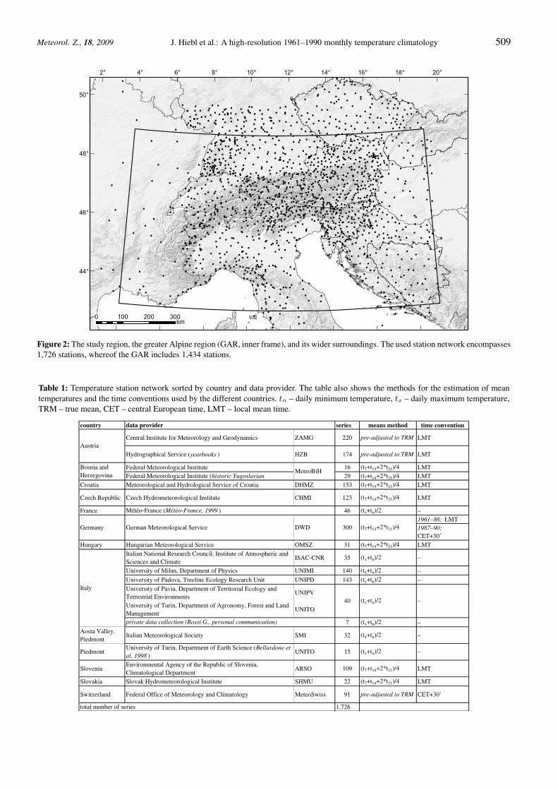
Figure 2: The study region, the greater Alpine region (GAR, inner frame), and its wider surroundings. The used station network encompasses1,726 stations, whereof the GAR includes 1,434 stations.
Table 1: Temperature station network sorted by country and data provider. The table also shows the methods for the estimation of meantemperatures and the time conventions used by the different countries. tn – daily minimum temperature, tx – daily maximum temperature,TRM – true mean, CET – central European time, LMT – local mean time.
country series means method time convention
Central Institute for Meteorology and Geodynamics ZAMG 220 pre-adjusted to TRM LMT
Hydrographical Service (yearbooks ) HZB 174 pre-adjusted to TRM LMT
Federal Meteorological Institute 16 (t7+t14+2*t21)/4 LMTFederal Meteorological Institute (historic Yugoslavian 29 (t7+t14+2*t21)/4 LMT
Croatia Meteorological and Hydrological Service of Croatia DHMZ 153 (t7+t14+2*t21)/4 LMT
Czech Republic Czech Hydrometeorological Institute CHMI 123 (t7+t14+2*t21)/4 LMT
France 46 (tx+tn)/2 –1961–86: LMT1987–90: CET+30’
Hungary Hungarian Meteorological Service OMSZ 31 (t7+t14+2*t21)/4 LMT
Italian National Research Council, Institute of Atmospheric and Sciences and Climate
ISAC-CNR 35 (tx+tn)/2 –
University of Milan, Department of Physics UNIMI 140 (tx+tn)/2 –
University of Padova, Treeline Ecology Research Unit UNIPD 143 (tx+tn)/2 –
University of Pavia, Department of Territorial Ecology and Terrestrial Environments
UNIPV
University of Turin, Department of Agronomy, Forest and Land Management
UNITO
7 (tx+tn)/2 –
Aosta Valley, Piedmont
Italian Meteorological Society SMI 32 (tx+tn)/2 –
SloveniaEnvironmental Agency of the Republic of Slovenia, Climatological Department
ARSO 109 (t7+t14+2*t21)/4 LMT
Slovakia Slovak Hydrometeorological Institute SHMU 22 (t7+t14+2*t21)/4 LMT
Switzerland Federal Office of Meteorology and Climatology MeteoSwiss 91 pre-adjusted to TRM CET+30’
1,726
University of Turin, Department of Earth Science (Bellardone et al. 1998 )
Piedmont UNITO 15 (tx+tn)/2
300 (t7+t14+2*t21)/4
Italy
–
total number of series
40 (tx+tn)/2 –
private data collection (Rossi G., personal communication)
data provider
Austria
Météo-France (Météo-France, 1999 )
Germany German Meteorological Service DWD
Bosnia and Herzegovina
MeteoBiH
eschweizerbartxxx ingenta

510 J. Hiebl et al.: A high-resolution 1961–1990 monthly temperature climatology Meteorol. Z., 18, 2009
08
11
1
2
912 10
10
37
13
5
76
64
18°16°14°12°10°8°6°4°
48°
46°
44°
Figure 3: Inhomogeneity adjustment subregions for the definitionof the daily temperature courses (DTCs) and the daily temperatureranges (DTRs), which were used for estimating the adjustmentsshown in Table 3. Most of these subregions were further dividedinto elevation bands. 0 = subregion with no need for adjustment,1 = extra-Alpine Austria, 2 = Alpine Austria, 3 = extra-AlpineSwitzerland, 4 = Jura, 5 = Alpine Switzerland, 6 = Engadin-Valais,7 = Alpine Italy, 8 = Po Plain, 9 = Apennine, 10 = coastal Italy,11 = North-eastern France, 12 = South-eastern France, 13 = coastalFrance.
and Herzegovina, Croatia, the Czech Republic, France,Germany, Hungary, Slovakia, Slovenia and Switzerland.These data were quality-tested 1961–1990 monthly cli-mate normals. An additional 24 % came from Italian re-gional and local data providers, mainly universities andother research institutes. The remaining 12 % of the datawere digitised from meteorological or hydrographicalyearbooks. The metadata review in Table 1 details thedata sources by country and their quantitative contribu-tions to the final dataset of 1,726 stations. This countconcerns an area which is actually slightly larger thanthe GAR and it includes only the stations, which passedthe first quality control.
Figure 2 shows the station network also highlightingthe borders of the 699,000 km2 region, that we define asGAR (4–19 ◦E and 43–49 ◦N). The GAR itself encom-passes 1,434 stations, corresponding to an average sta-tion distance of 22 km. Station density is rather homo-geneous over the study area, with two exceptions: Oneminor inhomogeneity is found along the borders of Hun-gary – but this can be regarded as less important, due tothe smooth Pannonian orography. More critical can bethe second drop in station density, visible in France. Themean station distances are 37 km for Hungary and 66 kmfor France, compared to only 19 km for the remainingpart of the GAR.
2.2 Homogenisation due to different methodsof means estimation
The patchy administrative structure of the study regionnot only caused huge work for data collection, but it alsoproduced breaks along national borders, due to differ-ent observing times and different methods for estimatingmean daily (and, consequently, monthly) temperatures.
The last two columns of Table 1 give more informationabout that. As different means formulas can cause dif-ferences of up to more than 1 ◦C, as we will show, theseinhomogeneities cannot be neglected.
Taking into account that the majority of the data(60 %) consists of mean temperatures based on the for-mula by KAMTZ (1860), namely tm = (t7 + t14 + 2 ∗
t21)/4, this calculus was chosen as the target, to whichthe means had to be adjusted. The decision against the(tx + tn)/2-calculus was based on the following reasons:Firstly, only 26 % of the data, i.e. those from Franceand Italy, were provided in this form and, secondly, the(tx + tn)/2-estimate deviates more than the other meth-ods from the true mean (TRM), which is given by con-tinuous hourly registration. So, we decided to re-adjustall the data, which were expressed in a different form, toKamtz-means. The basis for the identification of the ad-justments were subregional samples of records of hourlyobservations plus the two daily extremes. Such a basis isincreasingly available thanks to the ongoing automationof meteorological networks.
In the following we discuss how this issue was dealtwith, considering separately all countries, in which tem-peratures were not expressed according to the Kamtz-formula (Figure 3):
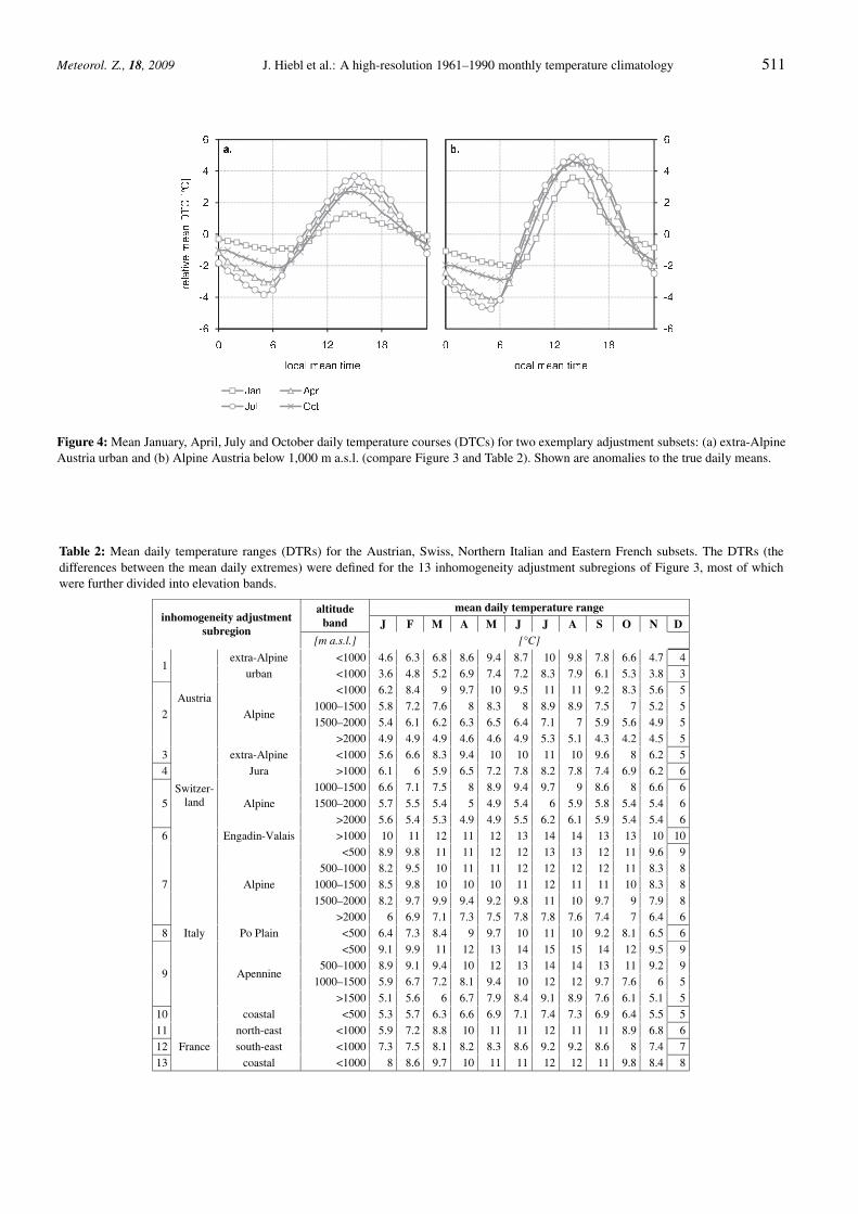
– The Austrian data consist of ZAMG and HZBrecords, which had already been gap-filled and ad-justed to the 1961–1990 period and to TRMs (AUERet al., 2001a). In order to re-adjust them to Kamtz-means, we considered a set of 100 records of hourlyobservations plus the two daily extremes (AT-T24-100 dataset). This dataset, which is similar to theone described in AUER et al. (2001a), allowed tostudy the mean daily temperature courses (DTCs)in six Austrian subregions (two extra-Alpine onesand an inner-Alpine one subdivided into four alti-tude bands). The DTCs, together with the mean dailytemperature ranges (DTRs), were used to derive cor-rections for the subsets with biased means. Figure 4shows examples of mean DTCs for two Austrian sta-tion subsets.
– Swiss data were provided by MeteoSwiss. They con-sist of monthly tm−, tx− and tn-means, tm eitherdirectly measured (ANETZ-sites) or pre-adjusted to(conventional sites) TRMs. In this case, the DTRswere already available, whereas the respective DTCswere produced by simply assuming the similarityof the shape of the DTCs in Austria and Switzer-land. The Swiss DTCs were calculated using Aus-trian DTCs, by modifying the DTCs’ amplitude bya multiplicative factor arising from the relation be-tween the respective DTRs. The available DTRs andthe estimated DTCs were used to re-adjust the Swissdata to Kamtz-means. For Switzerland the methodwas also verified by means of the ANETZ-stationrecords. The results were satisfactory (BEGERT M.,MeteoSwiss, personal communication), which madethe method seem appropriate for application in Italy
eschweizerbartxxx ingenta
Meteorol. Z., 18, 2009 J. Hiebl et al.: A high-resolution 1961–1990 monthly temperature climatology 511
Figure 4: Mean January, April, July and October daily temperature courses (DTCs) for two exemplary adjustment subsets: (a) extra-AlpineAustria urban and (b) Alpine Austria below 1,000 m a.s.l. (compare Figure 3 and Table 2). Shown are anomalies to the true daily means.
Table 2: Mean daily temperature ranges (DTRs) for the Austrian, Swiss, Northern Italian and Eastern French subsets. The DTRs (thedifferences between the mean daily extremes) were defined for the 13 inhomogeneity adjustment subregions of Figure 3, most of whichwere further divided into elevation bands.
inhomogeneity adjustment subregion
altitude band
mean daily temperature range
J F M A M J J A S O N D [m a.s.l.] [°C]
1
Austria
extra-Alpine <1000 4.6 6.3 6.8 8.6 9.4 8.7 10 9.8 7.8 6.6 4.7 4
urban <1000 3.6 4.8 5.2 6.9 7.4 7.2 8.3 7.9 6.1 5.3 3.8 3
2 Alpine
<1000 6.2 8.4 9 9.7 10 9.5 11 11 9.2 8.3 5.6 5
1000–1500 5.8 7.2 7.6 8 8.3 8 8.9 8.9 7.5 7 5.2 5
1500–2000 5.4 6.1 6.2 6.3 6.5 6.4 7.1 7 5.9 5.6 4.9 5
>2000 4.9 4.9 4.9 4.6 4.6 4.9 5.3 5.1 4.3 4.2 4.5 5
3
Switzer-land
extra-Alpine <1000 5.6 6.6 8.3 9.4 10 10 11 10 9.6 8 6.2 5
4 Jura >1000 6.1 6 5.9 6.5 7.2 7.8 8.2 7.8 7.4 6.9 6.2 6
5 Alpine
1000–1500 6.6 7.1 7.5 8 8.9 9.4 9.7 9 8.6 8 6.6 6
1500–2000 5.7 5.5 5.4 5 4.9 5.4 6 5.9 5.8 5.4 5.4 6
>2000 5.6 5.4 5.3 4.9 4.9 5.5 6.2 6.1 5.9 5.4 5.4 6
6 Engadin-Valais >1000 10 11 12 11 12 13 14 14 13 13 10 10
7
Italy
Alpine
<500 8.9 9.8 11 11 12 12 13 13 12 11 9.6 9
500–1000 8.2 9.5 10 11 11 12 12 12 12 11 8.3 8
1000–1500 8.5 9.8 10 10 10 11 12 11 11 10 8.3 8
1500–2000 8.2 9.7 9.9 9.4 9.2 9.8 11 10 9.7 9 7.9 8
>2000 6 6.9 7.1 7.3 7.5 7.8 7.8 7.6 7.4 7 6.4 6
8 Po Plain <500 6.4 7.3 8.4 9 9.7 10 11 10 9.2 8.1 6.5 6
9 Apennine
<500 9.1 9.9 11 12 13 14 15 15 14 12 9.5 9
500–1000 8.9 9.1 9.4 10 12 13 14 14 13 11 9.2 9
1000–1500 5.9 6.7 7.2 8.1 9.4 10 12 12 9.7 7.6 6 5
>1500 5.1 5.6 6 6.7 7.9 8.4 9.1 8.9 7.6 6.1 5.1 5
10 coastal <500 5.3 5.7 6.3 6.6 6.9 7.1 7.4 7.3 6.9 6.4 5.5 5
11
France
north-east <1000 5.9 7.2 8.8 10 11 11 12 11 11 8.9 6.8 6
12 south-east <1000 7.3 7.5 8.1 8.2 8.3 8.6 9.2 9.2 8.6 8 7.4 7
13 coastal <1000 8 8.6 9.7 10 11 11 12 12 11 9.8 8.4 8
eschweizerbartxxx ingenta
512 J. Hiebl et al.: A high-resolution 1961–1990 monthly temperature climatology Meteorol. Z., 18, 2009
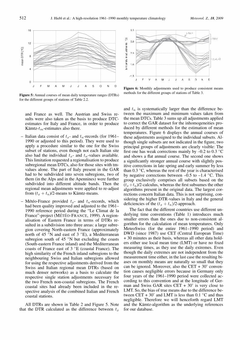
Figure 5: Annual courses of mean daily temperature ranges (DTRs)for the different groups of stations of Table 2.2.
and France as well. The Austrian and Swiss re-sults were also taken as the basis to produce DTC-estimates for Italy and France, in order to produceKamtz-tm-estimates also there.
– Italian data consist of tx- and tn-records (for 1961–1990 or adjusted to this period). They were used toapply a procedure similar to the one for the Swisssubset of stations, even though not each Italian sitealso had the individual tx- and tn-values available.This limitation requested a regionalisation to producesubregional mean DTCs, also for those sites with tm-values alone. The part of Italy present in the GARhad to be subdivided into seven subregions, two ofthem (in the Alps and in the Apennines) were furthersubdivided into different altitude bands. Then theregional mean adjustments were applied to re-adjustfrom (tx + tn)/2-means to Kamtz-means.
– Meteo-France provided tx- and tn-records, whichhad been quality improved and adjusted to the 1961–1990 reference period during the “Le Climat de laFrance”-project (METEO-FRANCE, 1999). A region-alisation of Eastern France in terms of DTRs re-sulted in a subdivision into three areas: a large subre-gion covering North-eastern France (approximatelynorth of 45 ◦N and east of 3 ◦E), a Mediterraneansubregion south of 45 ◦N but excluding the coasts(South-eastern France inland) and the Mediterraneancoasts of France east of 3 ◦E (coastal France). Thehigh similarity of the French inland subregions to theneighbouring Swiss and Italian subregions allowedfor using the respective adjustments derived from theSwiss and Italian regional mean DTRs (based onmuch denser networks) as a basis to calculate therespective single station adjustments necessary forthe two French non-coastal subregions. The Frenchcoastal sites had already been included in the re-spective analysis of the combined Italian and Frenchcoastal stations.
All DTRs are shown in Table 2 and Figure 5. Notethat the DTR calculated as the difference between tx
Figure 6: Monthly adjustments used to produce consistent meansmethods for the different groups of stations of Table 3.
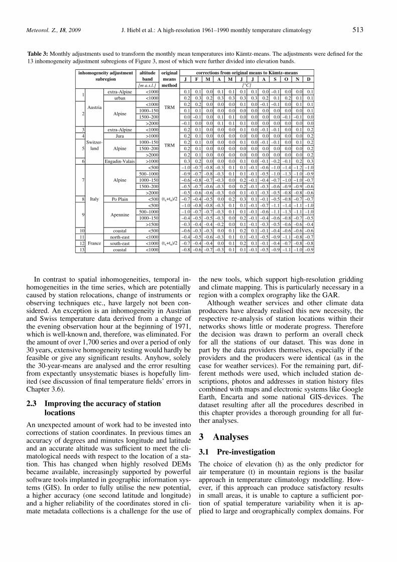
and tn is systematically larger than the difference be-tween the maximum and minimum values taken fromthe mean DTCs. Table 3 sums up all adjustments appliedto correct the GAR dataset for the inhomogeneities pro-duced by different methods for the estimation of meantemperatures. Figure 6 displays the annual courses ofthese adjustments assigned to the individual subsets. Al-though single subsets are not indicated in the figure, twoprincipal groups of adjustments are clearly visible: Thefirst one has weak corrections mainly by –0.2 to 0.3 ◦Cand shows a flat annual course. The second one showsa significantly stronger annual course with slightly pos-itive corrections in late spring and early summer by lessthan 0.3 ◦C, whereas the rest of the year is characterisedby negative corrections between –0.5 to –1.4 ◦C. Thisgroup exclusively comprises all subsets based on the(tx+tn)/2-calculus, whereas the first subsumes the otheralgorithms present in the original data. The largest cor-rections concern Italian data. This is not surprising, con-sidering the higher DTR-values in Italy and the generaldeficiencies of the (tx + tn)/2-approach.
The fact that the different countries use different un-derlying time conventions (Table 1) introduces muchsmaller errors than the ones due to non-consistent al-gorithm for the calculation of mean temperatures. OnlyMeteoSwiss (for the entire 1961–1990 period) andDWD (since 1987) use CET (Central European Time)+ 30 minutes as their basis, whereas all other data hold-ers either use local mean time (LMT) or have no fixedmeasuring times, as they use the daily extremes. Eventhough the daily extremes are not independent from themeasurement time either, in the last case the resulting bi-ases on monthly means are naturally so small that theycan be ignored. Moreover, also the CET + 30’ conven-tion causes negligible errors because in Germany onlyfour years of the 1961–1990 period were collected ac-cording to this convention and at the longitude of Ger-man and Swiss GAR sites CET + 30’ is very close toLMT. So, the bias of true means due to the difference be-tween CET + 30’ and LMT is less than 0.1 ◦C and thusnegligible. Therefore we will henceforth regard LMTand the Kamtz-algorithm as the underlying referencesfor our database.
eschweizerbartxxx ingenta
Meteorol. Z., 18, 2009 J. Hiebl et al.: A high-resolution 1961–1990 monthly temperature climatology 513
Table 3: Monthly adjustments used to transform the monthly mean temperatures into Kamtz-means. The adjustments were defined for the13 inhomogeneity adjustment subregions of Figure 3, most of which were further divided into elevation bands.
J F M A M J J A S O N D[m a.s.l.]
extra-Alpine <1000 0.1 0.1 0.0 0.1 0.1 0.1 0.1 0.0 –0.1 0.0 0.0 0.1urban <1000 0.2 0.3 0.2 0.3 0.3 0.3 0.3 0.2 0.1 0.2 0.1 0.1
<1000 0.2 0.2 0.0 0.0 0.0 0.1 0.0 –0.1 –0.1 0.0 0.1 0.11000–150 0.1 0.1 0.0 0.0 0.0 0.0 0.0 0.0 0.0 0.0 0.0 0.11500–200 0.0 –0.1 0.0 0.1 0.1 0.0 0.0 0.0 0.0 –0.1 –0.1 0.0
>2000 –0.1 0.0 0.0 0.1 0.1 0.1 0.0 0.0 0.0 0.0 0.0 0.03 extra-Alpine <1000 0.2 0.1 0.0 0.0 0.0 0.1 0.0 –0.1 –0.1 0.0 0.1 0.24 Jura >1000 0.2 0.1 0.0 0.0 0.0 0.0 0.0 0.0 0.0 0.0 0.0 0.2
1000–150 0.2 0.1 0.0 0.0 0.0 0.1 0.0 –0.1 –0.1 0.0 0.1 0.21500–200 0.2 0.1 0.0 0.0 0.0 0.0 0.0 0.0 0.0 0.0 0.0 0.2
>2000 0.2 0.1 0.0 0.0 0.0 0.0 0.0 0.0 0.0 0.0 0.0 0.26 Engadin-Valais >1000 0.3 0.2 0.0 0.0 0.0 0.1 0.0 –0.1 –0.2 –0.1 0.2 0.3
<500 –1.0 –0.7 –0.8 –0.3 0.1 0.1 –0.1 –0.6 –1.0 –1.4 –1.2 –1.0500–1000 –0.9 –0.7 –0.8 –0.3 0.1 0.1 –0.1 –0.5 –1.0 –1.3 –1.0 –0.91000–150 –0.6 –0.8 –0.7 –0.3 0.0 0.2 –0.1 –0.4 –0.7 –1.0 –1.0 –0.71500–200 –0.5 –0.7 –0.6 –0.3 0.0 0.2 –0.1 –0.3 –0.6 –0.9 –0.9 –0.6
>2000 –0.5 –0.6 –0.6 –0.3 0.0 0.1 –0.1 –0.3 –0.5 –0.8 –0.8 –0.68 Po Plain <500 –0.7 –0.4 –0.5 0.0 0.2 0.3 0.1 –0.1 –0.5 –0.8 –0.7 –0.7
<500 –1.0 –0.8 –0.8 –0.3 0.1 0.1 –0.1 –0.7 –1.1 –1.4 –1.1 –1.0500–1000 –1.0 –0.7 –0.7 –0.3 0.1 0.1 –0.1 –0.6 –1.1 –1.3 –1.1 –1.01000–150 –0.4 –0.5 –0.5 –0.3 0.0 0.2 –0.1 –0.4 –0.6 –0.8 –0.7 –0.5
>1500 –0.3 –0.4 –0.4 –0.2 0.0 0.1 –0.1 –0.3 –0.5 –0.6 –0.6 –0.410 coastal <500 –0.6 –0.3 –0.3 0.0 0.1 0.2 0.1 –0.1 –0.4 –0.6 –0.6 –0.611 north-east <1000 –0.4 –0.5 –0.6 –0.3 0.1 0.1 –0.1 –0.5 –0.9 –1.1 –0.8 –0.712 south-east <1000 –0.7 –0.4 –0.4 0.0 0.1 0.2 0.1 –0.1 –0.4 –0.7 –0.8 –0.813 coastal <1000 –0.8 –0.6 –0.7 –0.3 0.1 0.1 –0.1 –0.5 –0.9 –1.1 –1.0 –0.9
France (tx+tn)/2
Italy
Alpine
(tx+tn)/2
Alpine
7
9 Apennine
Switzer-land
TRM5
corrections from original means to Kämtz–means
[°C]
1
Austria TRM
inhomogeneity adjustment subregion
altitude band
original means
method
2 Alpine
In contrast to spatial inhomogeneities, temporal in-homogeneities in the time series, which are potentiallycaused by station relocations, change of instruments orobserving techniques etc., have largely not been con-sidered. An exception is an inhomogeneity in Austrianand Swiss temperature data derived from a change ofthe evening observation hour at the beginning of 1971,which is well-known and, therefore, was eliminated. Forthe amount of over 1,700 series and over a period of only30 years, extensive homogeneity testing would hardly befeasible or give any significant results. Anyhow, solelythe 30-year-means are analysed and the error resultingfrom expectantly unsystematic biases is hopefully lim-ited (see discussion of final temperature fields’ errors inChapter 3.6).
2.3 Improving the accuracy of stationlocations
An unexpected amount of work had to be invested intocorrections of station coordinates. In previous times anaccuracy of degrees and minutes longitude and latitudeand an accurate altitude was sufficient to meet the cli-matological needs with respect to the location of a sta-tion. This has changed when highly resolved DEMsbecame available, increasingly supported by powerfulsoftware tools implanted in geographic information sys-tems (GIS). In order to fully utilise the new potential,a higher accuracy (one second latitude and longitude)and a higher reliability of the coordinates stored in cli-mate metadata collections is a challenge for the use of
the new tools, which support high-resolution griddingand climate mapping. This is particularly necessary in aregion with a complex orography like the GAR.
Although weather services and other climate dataproducers have already realised this new necessity, therespective re-analysis of station locations within theirnetworks shows little or moderate progress. Thereforethe decision was drawn to perform an overall checkfor all the stations of our dataset. This was done inpart by the data providers themselves, especially if theproviders and the producers were identical (as in thecase for weather services). For the remaining part, dif-ferent methods were used, which included station de-scriptions, photos and addresses in station history filescombined with maps and electronic systems like GoogleEarth, Encarta and some national GIS-devices. Thedataset resulting after all the procedures described inthis chapter provides a thorough grounding for all fur-ther analyses.
3 Analyses
3.1 Pre-investigation
The choice of elevation (h) as the only predictor forair temperature (t) in mountain regions is the basilarapproach in temperature climatology modelling. How-ever, if this approach can produce satisfactory resultsin small areas, it is unable to capture a sufficient por-tion of spatial temperature variability when it is ap-plied to large and orographically complex domains. For
eschweizerbartxxx ingenta
514 J. Hiebl et al.: A high-resolution 1961–1990 monthly temperature climatology Meteorol. Z., 18, 2009
°
°
°°
°°
°
°°
°
°
° °
° °
° °
°
°
° °
° °
°
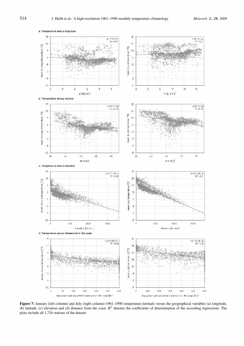
Figure 7: January (left column) and July (right column) 1961–1990 temperature normals versus the geographical variables (a) longitude,(b) latitude, (c) elevation and (d) distance from the coast. R2 denotes the coefficients of determination of the according regressions. Theplots include all 1,726 stations of the dataset.
eschweizerbartxxx ingenta
Meteorol. Z., 18, 2009 J. Hiebl et al.: A high-resolution 1961–1990 monthly temperature climatology 515
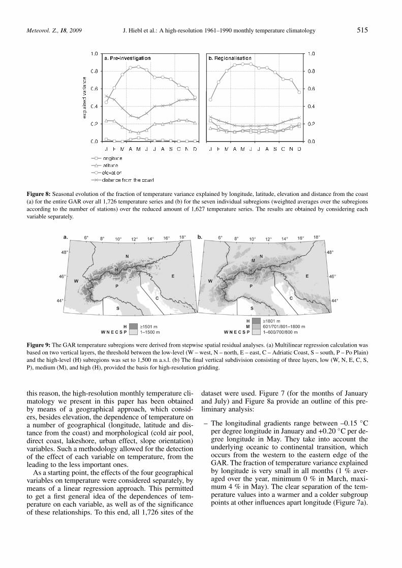
Figure 8: Seasonal evolution of the fraction of temperature variance explained by longitude, latitude, elevation and distance from the coast(a) for the entire GAR over all 1,726 temperature series and (b) for the seven individual subregions (weighted averages over the subregionsaccording to the number of stations) over the reduced amount of 1,627 temperature series. The results are obtained by considering eachvariable separately.
Figure 9: The GAR temperature subregions were derived from stepwise spatial residual analyses. (a) Multilinear regression calculation wasbased on two vertical layers, the threshold between the low-level (W – west, N – north, E – east, C – Adriatic Coast, S – south, P – Po Plain)and the high-level (H) subregions was set to 1,500 m a.s.l. (b) The final vertical subdivision consisting of three layers, low (W, N, E, C, S,P), medium (M), and high (H), provided the basis for high-resolution gridding.
this reason, the high-resolution monthly temperature cli-matology we present in this paper has been obtainedby means of a geographical approach, which consid-ers, besides elevation, the dependence of temperature ona number of geographical (longitude, latitude and dis-tance from the coast) and morphological (cold air pool,direct coast, lakeshore, urban effect, slope orientation)variables. Such a methodology allowed for the detectionof the effect of each variable on temperature, from theleading to the less important ones.
As a starting point, the effects of the four geographicalvariables on temperature were considered separately, bymeans of a linear regression approach. This permittedto get a first general idea of the dependences of tem-perature on each variable, as well as of the significanceof these relationships. To this end, all 1,726 sites of the
dataset were used. Figure 7 (for the months of Januaryand July) and Figure 8a provide an outline of this pre-liminary analysis:
– The longitudinal gradients range between –0.15 ◦Cper degree longitude in January and +0.20 ◦C per de-gree longitude in May. They take into account theunderlying oceanic to continental transition, whichoccurs from the western to the eastern edge of theGAR. The fraction of temperature variance explainedby longitude is very small in all months (1 % aver-aged over the year, minimum 0 % in March, maxi-mum 4 % in May). The clear separation of the tem-perature values into a warmer and a colder subgrouppoints at other influences apart longitude (Figure 7a).
eschweizerbartxxx ingenta
516 J. Hiebl et al.: A high-resolution 1961–1990 monthly temperature climatology Meteorol. Z., 18, 2009
– Latitudinal effects are considerably stronger andshow north-south gradients that range between–0.59 ◦C per degree latitude in May and –0.87 ◦Cper degree latitude in July. The fraction of tempera-ture variance explained by latitude is smallest in May(10 %) and largest in October (24 %). The averagefraction of the explained variance over all months is19 %. The clear deviations of the temperature nor-mals from a linear course, as well as the large partof unexplained variance, characterise also the depen-dence on latitude alone as insufficient (Figure 7b).
– As expected, the highest explained variance is achie-ved by the vertical regression model. Elevation vari-ations explain as much as 69 % of temperature vari-ance averaged over the year, reaching the maximumexplained value in May (85 %). During winter stableatmospheric layering is responsible for a reduced sig-nificance of the elevation effect (only 45 % of vari-ance explained in January). January turns also outto be the month with the lowest vertical lapse rateof temperature (–0.42 ◦C/100m), whereas the high-est value is found in May (–0.62 ◦C/100m). Even thevertical model alone produces residuals up to ±5 ◦Cat a given altitude. During winter, non-linear regres-sion would better fit the distribution of temperaturewith elevation (Figure 7c).
– In order to capture maritime influences, a field of dis-tances from the coast was established. Taking intoaccount the fact that such dependence is criticallysensitive to the orographical obstacles between eachpoint and the nearest coast, such distances were to-pographically weighted. Moreover, a fixed value wasassigned to all points of coast distance over a thresh-old and their values simply set equal to the thresh-old itself. The dependence of temperature on distancefrom the coast is surprisingly strong. Considering theaverage over all months, it explains 41 % of the vari-ance of the temperature normals – more than longi-tude or latitude. There is also a clear seasonal signalwith higher values of explained variance during thecold season (maximum 52 % in January) and lowervalues during the warm season (minimum 27 % inMay). Per 100 topographically weighted kilometresfrom the coast, the temperature decreases between–1.02 ◦C in January and –0.78 ◦C in May (Figure7d). The strength of the coast distance effect, as wellas the all-season inland temperature decrease, giveclear evidence of other influences superimposed tothe large-scale coast effect – an inconsistency thathad to be eliminated towards the finalised tempera-ture model.
The results of the preliminary analyses on the tem-perature dependence on longitude, latitude, elevationand distance from the coast highlight that each of thefour variables contains the potential to contribute to themodelling of Alpine temperature variability. Neverthe-less, size and distribution of the residuals underline the
necessity for refinements beyond a simple linear regres-sion approach over the entire study region. With thisunderstanding, the methodical schedule for the furtherworking steps was determined: (i) Instead of regardingthe entire GAR as a whole, the study region was dividedinto a number of subregions (Chapter 3.2). (ii) A mul-tilinear regression approach of temperature against lon-gitude, latitude, elevation and distance from the coastshould supersede separate linear regressions (Chapter3.3). (iii) Still remaining temperature climate features,uncaptured by the multilinear regression, should be con-sidered by tailored procedures (Chapter 3.5).
3.2 Regionalisation
As many conflicting climate regimes interact over theAlps and its surroundings, large quality improvement inthe modelling of temperature distribution was expectedfrom dividing the GAR into further horizontal and ver-tical subregions (Figure 9a). Regionalisation was basedon stepwise spatial residual analyses. In terms of hori-zontal subdivision, four subregions constitute the cardi-nal directions and encompass the forelands to the west(W), north (N) and east of the Alps (E) and to the southof the Apennines (S). Two particular subregions copewith the geographic characteristics of the Adriatic area,one covering the mainly enclosed Po Plain including thewestern Adriatic coast (P), the other one comprehend-ing the eastern Adriatic coast (C). Well-founded bordersbetween the climate subregions could easily be locatedalong the main Apennine, Alpine and Dinaric crests.The identification of the optimal border around the areaof Friuli and Istria, however, required numerous trialsof tentative temperature modelling, before a satisfactorysolution was found. For the vertical subdivision, two lay-ers were initially separated at 1,500 m a.s.l. Underneaththis level the six horizontal subregions were present,whereas all other, high-Alpine stations were gatheredto one single high-elevation layer (H). This initial ver-tical subdivision was to be refined later (Chapter 3.4).The resulting GAR subregions reflect real climatologicinfluences. In this way, unlike many existing climatolo-gies, the temperature fields are not artificially cut off atnational borders, which often gives rise to problematicboundary effects.
Solely to demonstrate the improvement produced bythe regionalisation, simple regressions have been calcu-lated again, but now separately for the seven individ-ual subregions and over the reduced amount of 1,627temperature series. The resulting explained variances,weighted according to the number of stations per sub-region, are shown in Figure 8b. They highlight that thesubdivision into different subregions allows to bettercapture the temperature dependence on the geographi-cal variables. The comparison of the subplots in Figure 8shows that:
eschweizerbartxxx ingenta
Meteorol. Z., 18, 2009 J. Hiebl et al.: A high-resolution 1961–1990 monthly temperature climatology 517
?? hhff dd
19°E4°E 43°N 49°N 1 4,570 m 0 600 units
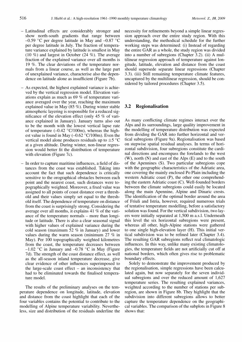
Figure 10: Spatial variation of the four geographical variables, which serve as independent variables in the multilinear regression withtemperature (t): longitude (λ), latitude (ϕ), elevation (h) and topographically weighted distance from the coast (d).
– Although longitude still makes the smallest contribu-tion of the four variables in terms of explained vari-ance, it is clearly stronger than before the regional-isation. Averaged over the year, the explained tem-perature variance by longitude now reaches a valueof 14 %. The extreme values occur in January (24 %)and July (10 %), fitting well the idea of a strongeroceanic-continental temperature gradient during thecold season.
– Similarly, about 14 % of temperature variance arecaptured by latitudinal changes in terms of the subre-gional regressions. Common variance is smallest inApril (11 %) and largest in December (18 %).
– After the regionalisation, the relevance of elevationfor air temperature is slightly higher. Elevation dif-ferences are responsible for as much as 75 % of thetemperature variance averaged over the year, the ac-cording monthly values range from 48 % in Januaryto 88 % in May.
– Distance from the coast remains the second mostimportant variable but explains considerably less,namely 21 %, of temperature variances after region-alisation. Nevertheless, the clear seasonality in theexplained variances persists (maximum 28 % in Jan-uary, minimum 17 % in July). Apparently, the strongnon-regionalised “coastal effect” was partly due tolatitudinal effects because coasts are exclusively lo-cated in the southern parts of the GAR.
Summarising, the regionalisation improved and gavemore consistency to the different geographical variables,that now show more reasonable annual courses and aremore coherent with the importance of their effect ontemperature. In particular, the coast effect was reducedto a more reasonable value to the advantage of the othervariables. We conclude that this type of regionalisationprovides a well-grounded basis for the calculation ofmultilinear regressions.
3.3 Multilinear regression
In order to overcome the limits of the linear regressionsbased on single variables, a multilinear regression of
Figure 11: Temperature versus elevation for the GAR stations inJanuary. To avoid artificial temperature breaks at 1,500 m a.s.l., thetwo-layer-model (grey lines) was refined and a three-layer-model(black lines) was introduced. It was developed by setting the low-elevation layers’ upper limit at 600, 700 or 800 m and the high-elevation layer’s lower limit at 1,800 m and by linearly interpolatingin between.
temperature versus longitude, latitude, elevation and dis-tance from the coast was performed for each subregionof the GAR and every month of the year (Figure 10). Theresulting regression equations underlie the finalised tem-perature climatology. In terms of the multilinear regres-sions, the geographical variables show consistent annualcycles of explained temperature variance:
– Longitude explains the eastward decreasing Atlanticand increasing continental influences on air temper-ature in the GAR. Averaged over all subregions,the west-east component accounts for temperaturechanges, which range from –0.21 ◦C per degree lon-gitude in January to +0.09 ◦C per degree longitude inMay.
– Latitude captures the effect of the south-north solarradiation gradient on temperature. It clearly explainsthe northward temperature decrease in all months andcauses temperature changes ranging from –0.64 ◦Cper degree latitude in late autumn to –0.37 ◦C perdegree latitude in late spring.
eschweizerbartxxx ingenta
518 J. Hiebl et al.: A high-resolution 1961–1990 monthly temperature climatology Meteorol. Z., 18, 2009
– Temperature decrease with increasing elevation variesregionally and seasonally, too. Averaged over allGAR subregions, the strongest vertical lapse ratesoccur from mid-spring to late-summer (maximum–0.63 ◦C per 100 m in April) and the weakest onesfrom mid-autumn to mid-winter (minimum –0.32 ◦Cper 100 m in January). As already mentioned, thesedistinct seasonal lapse rates correspond to more tur-bulent convective conditions in the warm season andmore stable conditions with inversions in the coldseason.
– Proximity to the sea mainly causes an increase ofwinter temperatures and a minor decrease of summertemperatures. January temperatures usually fall by–0.30 ◦C per 100 topographically weighted kilome-tres from the coast, whereas July temperatures neg-ligibly rise by +0.03 ◦C. It is worth noting thatthe coast distance temperature gradients obtained bymeans of the multilinear approach are more realisticthan the ones obtained by means of the simple linearregression.
3.4 Revised regionalisation
The main problem in constructing a multiregional clima-tology is that the use of different regression equationsmay arouse problems when the individual subregionaltemperature fields are merged together. Artificial tem-perature breaks at borders separating the subregions maybe present. In fact, this problem was not evident for theGAR horizontal subregions. Even along the long bordersrunning through the lowland, only negligible tempera-ture shifts occurred throughout. Only at the rather shortand uncertain border between subregions P and C inFriuli, temperature breaks required subsequent smooth-ing in winter months.
In contrast, important discontinuities appeared at thevertical border between the low- and the high-elevationsubregions at 1,500 m a.s.l, with a break of about 2to 3 ◦C in January (Figure 11). They were due to thefact that the model containing only two vertical subre-gions for the description of temperature reduction withincreasing elevation (i.e. linear decrease with differentslopes) was not able to satisfactory describe all relevantaspects of the irregular temperature dependence on el-evation. The distribution of the individual station val-ues of temperature-elevation-relationships as indicatedin Figure 11 suggests that ideally an asymmetric inversetangent-like curve would fit real temperature reductionwith increasing elevation in the lower atmosphere best.BRUNETTI et al. (2009) and SPINONI et al. (2008) avoidthe same problem in their Northern Italian climatologyby replacing the two-layer-model by a single linear re-gression over the whole elevation range.
For the GAR climatology, the problem was solved byestablishing a third vertical layer (M), visible in lightgrey on the map of Figure 9b. It was introduced toconnect the low-level and high-level regression lines.To this end, the low-elevation layers’ upper limit was
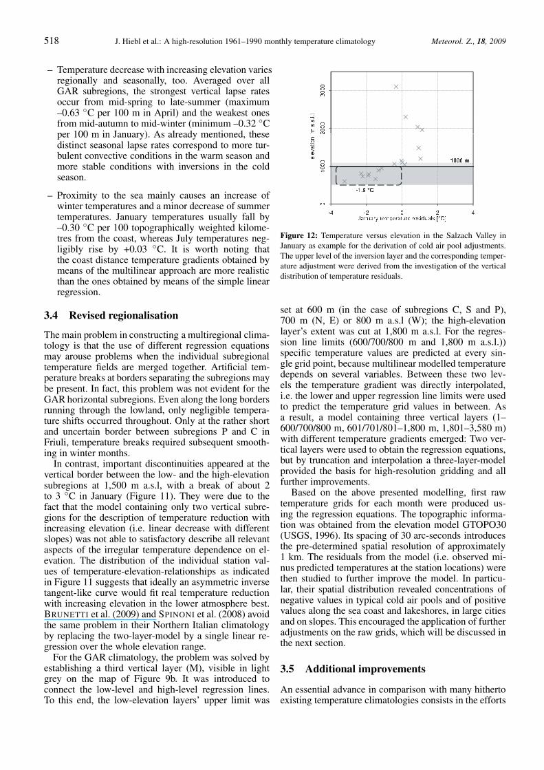
Figure 12: Temperature versus elevation in the Salzach Valley inJanuary as example for the derivation of cold air pool adjustments.The upper level of the inversion layer and the corresponding temper-ature adjustment were derived from the investigation of the verticaldistribution of temperature residuals.
set at 600 m (in the case of subregions C, S and P),700 m (N, E) or 800 m a.s.l (W); the high-elevationlayer’s extent was cut at 1,800 m a.s.l. For the regres-sion line limits (600/700/800 m and 1,800 m a.s.l.))specific temperature values are predicted at every sin-gle grid point, because multilinear modelled temperaturedepends on several variables. Between these two lev-els the temperature gradient was directly interpolated,i.e. the lower and upper regression line limits were usedto predict the temperature grid values in between. Asa result, a model containing three vertical layers (1–600/700/800 m, 601/701/801–1,800 m, 1,801–3,580 m)with different temperature gradients emerged: Two ver-tical layers were used to obtain the regression equations,but by truncation and interpolation a three-layer-modelprovided the basis for high-resolution gridding and allfurther improvements.
Based on the above presented modelling, first rawtemperature grids for each month were produced us-ing the regression equations. The topographic informa-tion was obtained from the elevation model GTOPO30(USGS, 1996). Its spacing of 30 arc-seconds introducesthe pre-determined spatial resolution of approximately1 km. The residuals from the model (i.e. observed mi-nus predicted temperatures at the station locations) werethen studied to further improve the model. In particu-lar, their spatial distribution revealed concentrations ofnegative values in typical cold air pools and of positivevalues along the sea coast and lakeshores, in large citiesand on slopes. This encouraged the application of furtheradjustments on the raw grids, which will be discussed inthe next section.
3.5 Additional improvements
An essential advance in comparison with many hithertoexisting temperature climatologies consists in the efforts
eschweizerbartxxx ingenta
Meteorol. Z., 18, 2009 J. Hiebl et al.: A high-resolution 1961–1990 monthly temperature climatology 519°
°
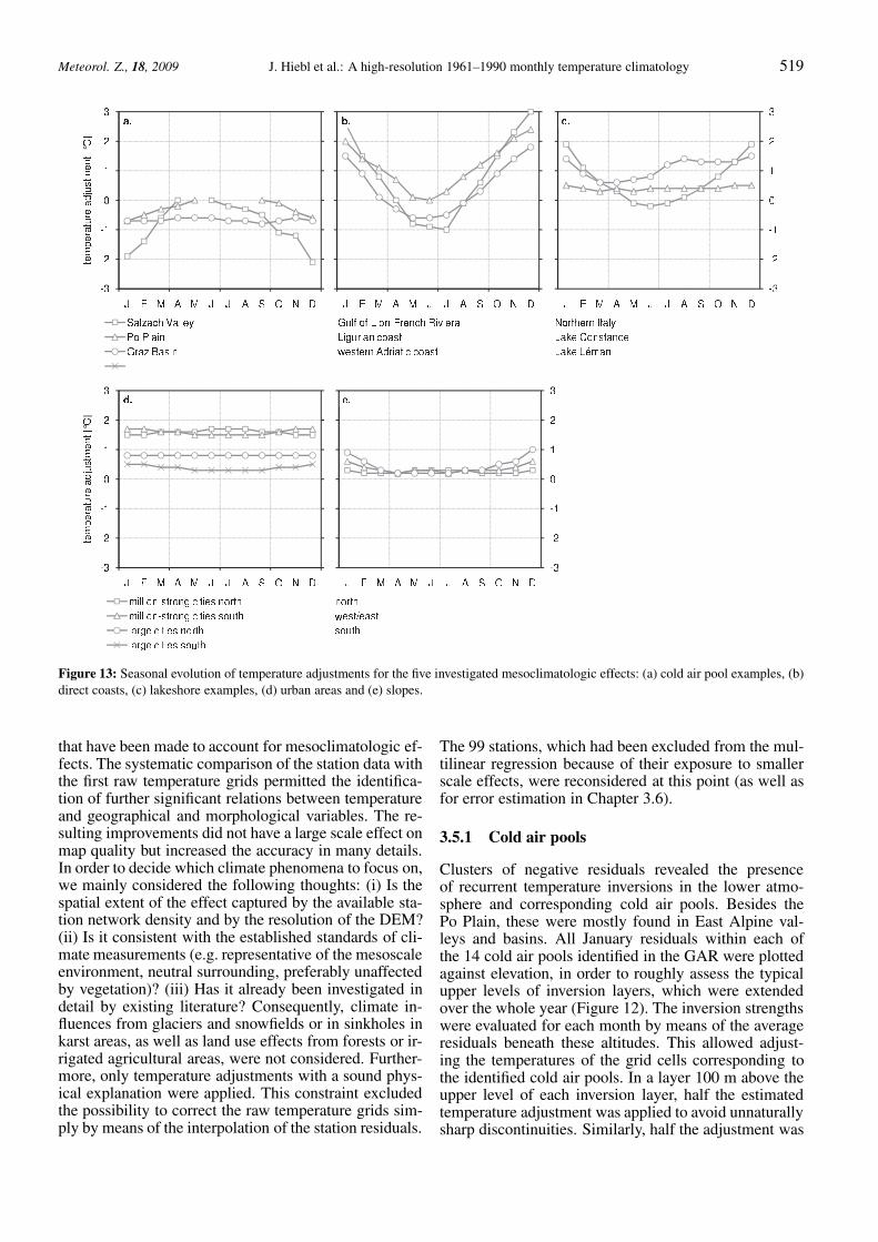
Figure 13: Seasonal evolution of temperature adjustments for the five investigated mesoclimatologic effects: (a) cold air pool examples, (b)direct coasts, (c) lakeshore examples, (d) urban areas and (e) slopes.
that have been made to account for mesoclimatologic ef-fects. The systematic comparison of the station data withthe first raw temperature grids permitted the identifica-tion of further significant relations between temperatureand geographical and morphological variables. The re-sulting improvements did not have a large scale effect onmap quality but increased the accuracy in many details.In order to decide which climate phenomena to focus on,we mainly considered the following thoughts: (i) Is thespatial extent of the effect captured by the available sta-tion network density and by the resolution of the DEM?(ii) Is it consistent with the established standards of cli-mate measurements (e.g. representative of the mesoscaleenvironment, neutral surrounding, preferably unaffectedby vegetation)? (iii) Has it already been investigated indetail by existing literature? Consequently, climate in-fluences from glaciers and snowfields or in sinkholes inkarst areas, as well as land use effects from forests or ir-rigated agricultural areas, were not considered. Further-more, only temperature adjustments with a sound phys-ical explanation were applied. This constraint excludedthe possibility to correct the raw temperature grids sim-ply by means of the interpolation of the station residuals.
The 99 stations, which had been excluded from the mul-tilinear regression because of their exposure to smallerscale effects, were reconsidered at this point (as well asfor error estimation in Chapter 3.6).
3.5.1 Cold air pools
Clusters of negative residuals revealed the presenceof recurrent temperature inversions in the lower atmo-sphere and corresponding cold air pools. Besides thePo Plain, these were mostly found in East Alpine val-leys and basins. All January residuals within each ofthe 14 cold air pools identified in the GAR were plottedagainst elevation, in order to roughly assess the typicalupper levels of inversion layers, which were extendedover the whole year (Figure 12). The inversion strengthswere evaluated for each month by means of the averageresiduals beneath these altitudes. This allowed adjust-ing the temperatures of the grid cells corresponding tothe identified cold air pools. In a layer 100 m above theupper level of each inversion layer, half the estimatedtemperature adjustment was applied to avoid unnaturallysharp discontinuities. Similarly, half the adjustment was
eschweizerbartxxx ingenta

520 J. Hiebl et al.: A high-resolution 1961–1990 monthly temperature climatology Meteorol. Z., 18, 2009
SalzburgSalzburg
RadstadtRadstadt
KufsteinKufstein
SonnblickSonnblick
Zell am SeeZell am See
ToulonToulon
CannesCannes
Le LucLe Luc
Cap CamaratCap Camarat
Saint-RaphaëlSaint-Raphaël
ComoComo
LuganoLugano
BergamoBergamo
LocarnoLocarno
VerbaniaVerbania
ChiavennaChiavenna
Milano-MalpensaMilano-Malpensa
WienWien
BadenBaden
MalackyMalacky
NeusiedlNeusiedl
HollabrunnHollabrunn
Wiener NeustadtWiener Neustadt
Bratislava-KolybaBratislava-Kolyba
BormioBormio
BergamoBergamo
SamedanSamedan
SondrioSondrio
ChiavennaChiavenna
SalzburgSalzburg
RadstadtRadstadt
KufsteinKufstein
SonnblickSonnblick
Zell am SeeZell am See
BormioBormio
BergamoBergamo
SamedanSamedan
SondrioSondrio
ChiavennaChiavenna
WienWien
BadenBaden
MalackyMalacky
NeusiedlNeusiedl
HollabrunnHollabrunn
Wiener NeustadtWiener Neustadt
Bratislava-KolybaBratislava-Kolyba
ComoComo
LuganoLugano
BergamoBergamo
LocarnoLocarno
VerbaniaVerbania
ChiavennaChiavenna
Milano-MalpensaMilano-Malpensa
ToulonToulon
CannesCannes
Le LucLe Luc
Cap CamaratCap Camarat
Saint-RaphaëlSaint-Raphaël
a.
b.
c.
d.
e.
SalzburgSalzburg
RadstadtRadstadt
KufsteinKufstein
SonnblickSonnblick
Zell am SeeZell am See
ToulonToulon
CannesCannes
Le LucLe Luc
Cap CamaratCap Camarat
Saint-RaphaëlSaint-Raphaël
ComoComo
LuganoLugano
BergamoBergamo
LocarnoLocarno
VerbaniaVerbania
ChiavennaChiavenna
Milano-MalpensaMilano-Malpensa
WienWien
BadenBaden
MalackyMalacky
NeusiedlNeusiedl
HollabrunnHollabrunn
Wiener NeustadtWiener Neustadt
Bratislava-KolybaBratislava-Kolyba
BormioBormio
BergamoBergamo
SamedanSamedan
SondrioSondrio
ChiavennaChiavenna
0 20 40km
Mean monthly air temperature (°C) -12 -10 -8 -6 -4 -2 0 2 4 6 8 10 -3 -2 -1 0 +1 +2 +3
Temperature adjustment (°C)
Figure 14: Map sections depicting raw temperature fields (left column), applied adjustments (central column) and adjusted temperaturefields (right column) as examples for (a) the cold air pool effect (Salzach Valley in January), (b) the direct coast effect (French Riviera inDecember), (c) the lakeshore effect (Northern Italy in February) (d) the urban effect (Vienna and Bratislava in October) and (e) the slopeeffects (Valtellina in December) respectively.
eschweizerbartxxx ingenta
Meteorol. Z., 18, 2009 J. Hiebl et al.: A high-resolution 1961–1990 monthly temperature climatology 521
applied at the lower end, i.e. at the outlet of a valleyor around the open edge of a basin. The total numberof considered records was 307; city stations, likely tobe affected by an urban warming effect, were excludedfrom the cold air pool analysis. When positive adjust-ments resulted, which was rarely the case during sum-mer months, these always small values were ignored dueto the lack of a physical justification for positive correc-tions.
The resulting temperature adjustments met the expec-tations both in size and seasonality and, thus, confirmedthe suitability of this approach. Figure 13a shows threeexamples: The largest corrections were applied to closedvalleys of the inner Alps like Swiss high valleys (UpperEngadin, Hinterrhein and Urseren) and Salzach Valleybut also to Cadore in the northernmost part of Veneto.These cold air pools usually show adjustments charac-terised by distinct annual amplitudes with a strong signalduring winter and a weaker one during summer. Gener-ally weaker adjustments were necessary for the Po Plainand Trentino, where the cold air pools are present only inthe winter season. On the contrary, in broad valleys andbasins on the eastern edge of the Alps, e.g. in the Ennsand Mura Valleys and the Graz Basin, weak inversionsconsist rather permanently throughout the year. Over allaffected valleys and basins, the applied temperature ad-justments range from –2.6 to –0.4 ◦C in December to–0.7 to 0.0 ◦C in June and July. No clear hints for cold airpools at all could be found in the records from the west-ern and south-western parts of the Alps. There, atmo-spheric turbulence in the proximity to the sea, togetherwith the smaller extension of the Alps perpendicular totheir length-axis, seem to hinder the formation of persis-tent cold air pools even during the winter months. As avisual example of the differences between raw and cold-air-pool-adjusted temperature maps, the situation of theSalzach Valley is shown in Figure 14a. It is worth notic-ing that in the final temperature map mid-elevation slopelocations appear warmer than lower and higher valleyregions – a well known effect caused by the downwardflow of heavier cold air.
3.5.2 Direct coasts
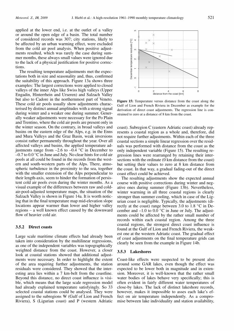
Large scale maritime climate effects had already beentaken into consideration by the multilinear regressions,as one of the independent variables was topographicallyweighted distance from the coast. However, a closerlook at coastal stations showed that additional adjust-ments were necessary. In order to highlight the extentof the area requiring further adjustments, the stationresiduals were considered. They showed that the inter-esting area lies within a 7 km-belt from the coastline.Beyond this distance, no direct coast influence is visi-ble, which means that the large scale regression modelhad already explained temperature satisfyingly. So 33selected coastal stations could be analysed. They wereassigned to the subregions W (Gulf of Lion and FrenchRiviera), S (Ligurian coast) and P (western Adriatic
Figure 15: Temperature versus distance from the coast along theGulf of Lion and French Riviera in December as example for thederivation of direct coast adjustments. The regression line is con-strained to zero at a distance of 8 km from the coast.
coast). Subregion C (eastern Adriatic coast) already rep-resents a coastal region as a whole and, therefore, didnot require further adjustments. Within each of the threecoastal sections a simple linear regression over the resid-uals was performed with distance from the coast as theonly independent variable (Figure 15). The resulting re-gression lines were rearranged by retaining their inter-sections with the ordinate (0 km distance from the coast)but setting their values to zero at 8 km distance fromthe coast. In that way, a gradual fading-out of the directcoast effect could be achieved.
The resulting adjustments show the expected annualcourse with positive corrections during winter and neg-ative ones during summer (Figure 13b). Nevertheless,winter warming in all three coastal regions is clearlystronger than summer cooling, which in case of the Lig-urian coast is negligible. Typically, the adjustments (di-rectly at the coast) range between 3.0 to 1.8 ◦C in De-cember and –1.0 to 0.0 ◦C in June or July. The adjust-ments could be affected by the rather small number ofrecords within each coastal region. Among the threecoastal regions, the strongest direct coast influence isfound at the Gulf of Lion and French Riviera, the weak-est one at the western Adriatic coast. The gradual effectof coast adjustments on the final temperature grids canclearly be seen from the example in Figure 14b.
3.5.3 Lakeshores
Coast-like effects were suspected to be present alsoaround some GAR lakes, even though the effect wasexpected to be lower both in magnitude and in exten-sion. Moreover, it is well-known that the rather smallwater bodies of lakes behave very specifically; this isoften evident in fairly different water temperatures ofclose-by lakes. The lack of distinct lakeshore records,however, makes it impossible to asses each lake’s ef-fect on air temperature independently. As a compro-mise between lake individuality and station availability,
eschweizerbartxxx ingenta
522 J. Hiebl et al.: A high-resolution 1961–1990 monthly temperature climatology Meteorol. Z., 18, 2009
°° °
°
° °
° °
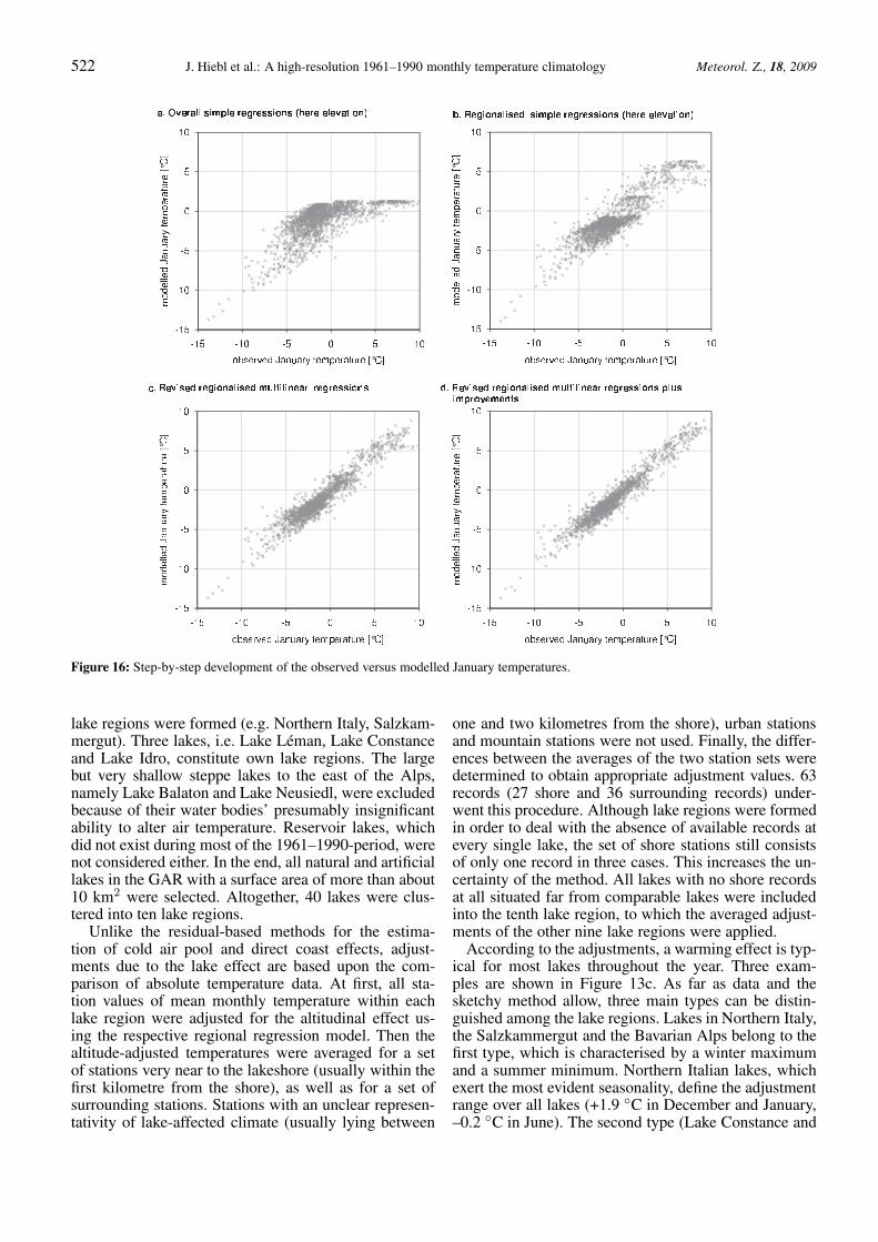
Figure 16: Step-by-step development of the observed versus modelled January temperatures.
lake regions were formed (e.g. Northern Italy, Salzkam-mergut). Three lakes, i.e. Lake Leman, Lake Constanceand Lake Idro, constitute own lake regions. The largebut very shallow steppe lakes to the east of the Alps,namely Lake Balaton and Lake Neusiedl, were excludedbecause of their water bodies’ presumably insignificantability to alter air temperature. Reservoir lakes, whichdid not exist during most of the 1961–1990-period, werenot considered either. In the end, all natural and artificiallakes in the GAR with a surface area of more than about10 km2 were selected. Altogether, 40 lakes were clus-tered into ten lake regions.
Unlike the residual-based methods for the estima-tion of cold air pool and direct coast effects, adjust-ments due to the lake effect are based upon the com-parison of absolute temperature data. At first, all sta-tion values of mean monthly temperature within eachlake region were adjusted for the altitudinal effect us-ing the respective regional regression model. Then thealtitude-adjusted temperatures were averaged for a setof stations very near to the lakeshore (usually within thefirst kilometre from the shore), as well as for a set ofsurrounding stations. Stations with an unclear represen-tativity of lake-affected climate (usually lying between
one and two kilometres from the shore), urban stationsand mountain stations were not used. Finally, the differ-ences between the averages of the two station sets weredetermined to obtain appropriate adjustment values. 63records (27 shore and 36 surrounding records) under-went this procedure. Although lake regions were formedin order to deal with the absence of available records atevery single lake, the set of shore stations still consistsof only one record in three cases. This increases the un-certainty of the method. All lakes with no shore recordsat all situated far from comparable lakes were includedinto the tenth lake region, to which the averaged adjust-ments of the other nine lake regions were applied.
According to the adjustments, a warming effect is typ-ical for most lakes throughout the year. Three exam-ples are shown in Figure 13c. As far as data and thesketchy method allow, three main types can be distin-guished among the lake regions. Lakes in Northern Italy,the Salzkammergut and the Bavarian Alps belong to thefirst type, which is characterised by a winter maximumand a summer minimum. Northern Italian lakes, whichexert the most evident seasonality, define the adjustmentrange over all lakes (+1.9 ◦C in December and January,–0.2 ◦C in June). The second type (Lake Constance and
eschweizerbartxxx ingenta
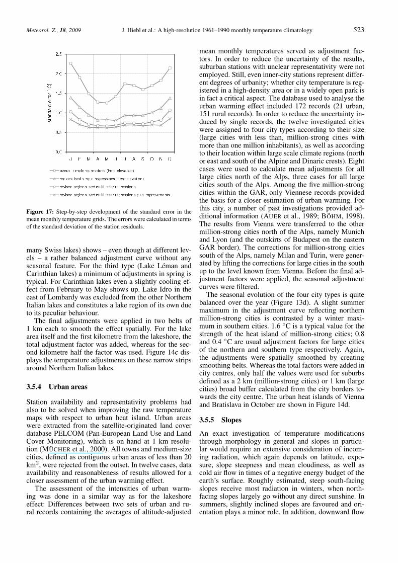
Meteorol. Z., 18, 2009 J. Hiebl et al.: A high-resolution 1961–1990 monthly temperature climatology 523
Figure 17: Step-by-step development of the standard error in themean monthly temperature grids. The errors were calculated in termsof the standard deviation of the station residuals.
many Swiss lakes) shows – even though at different lev-els – a rather balanced adjustment curve without anyseasonal feature. For the third type (Lake Leman andCarinthian lakes) a minimum of adjustments in spring istypical. For Carinthian lakes even a slightly cooling ef-fect from February to May shows up. Lake Idro in theeast of Lombardy was excluded from the other NorthernItalian lakes and constitutes a lake region of its own dueto its peculiar behaviour.
The final adjustments were applied in two belts of1 km each to smooth the effect spatially. For the lakearea itself and the first kilometre from the lakeshore, thetotal adjustment factor was added, whereas for the sec-ond kilometre half the factor was used. Figure 14c dis-plays the temperature adjustments on these narrow stripsaround Northern Italian lakes.
3.5.4 Urban areas
Station availability and representativity problems hadalso to be solved when improving the raw temperaturemaps with respect to urban heat island. Urban areaswere extracted from the satellite-originated land coverdatabase PELCOM (Pan-European Land Use and LandCover Monitoring), which is on hand at 1 km resolu-tion (MUCHER et al., 2000). All towns and medium-sizecities, defined as contiguous urban areas of less than 20km2, were rejected from the outset. In twelve cases, dataavailability and reasonableness of results allowed for acloser assessment of the urban warming effect.
The assessment of the intensities of urban warm-ing was done in a similar way as for the lakeshoreeffect: Differences between two sets of urban and ru-ral records containing the averages of altitude-adjusted
mean monthly temperatures served as adjustment fac-tors. In order to reduce the uncertainty of the results,suburban stations with unclear representativity were notemployed. Still, even inner-city stations represent differ-ent degrees of urbanity; whether city temperature is reg-istered in a high-density area or in a widely open park isin fact a critical aspect. The database used to analyse theurban warming effect included 172 records (21 urban,151 rural records). In order to reduce the uncertainty in-duced by single records, the twelve investigated citieswere assigned to four city types according to their size(large cities with less than, million-strong cities withmore than one million inhabitants), as well as accordingto their location within large scale climate regions (northor east and south of the Alpine and Dinaric crests). Eightcases were used to calculate mean adjustments for alllarge cities north of the Alps, three cases for all largecities south of the Alps. Among the five million-strongcities within the GAR, only Viennese records providedthe basis for a closer estimation of urban warming. Forthis city, a number of past investigations provided ad-ditional information (AUER et al., 1989; BOHM, 1998).The results from Vienna were transferred to the othermillion-strong cities north of the Alps, namely Munichand Lyon (and the outskirts of Budapest on the easternGAR border). The corrections for million-strong citiessouth of the Alps, namely Milan and Turin, were gener-ated by lifting the corrections for large cities in the southup to the level known from Vienna. Before the final ad-justment factors were applied, the seasonal adjustmentcurves were filtered.
The seasonal evolution of the four city types is quitebalanced over the year (Figure 13d). A slight summermaximum in the adjustment curve reflecting northernmillion-strong cities is contrasted by a winter maxi-mum in southern cities. 1.6 ◦C is a typical value for thestrength of the heat island of million-strong cities; 0.8and 0.4 ◦C are usual adjustment factors for large citiesof the northern and southern type respectively. Again,the adjustments were spatially smoothed by creatingsmoothing belts. Whereas the total factors were added incity centres, only half the values were used for suburbsdefined as a 2 km (million-strong cities) or 1 km (largecities) broad buffer calculated from the city borders to-wards the city centre. The urban heat islands of Viennaand Bratislava in October are shown in Figure 14d.
3.5.5 Slopes
An exact investigation of temperature modificationsthrough morphology in general and slopes in particu-lar would require an extensive consideration of incom-ing radiation, which again depends on latitude, expo-sure, slope steepness and mean cloudiness, as well ascold air flow in times of a negative energy budget of theearth’s surface. Roughly estimated, steep south-facingslopes receive most radiation in winters, when north-facing slopes largely go without any direct sunshine. Insummers, slightly inclined slopes are favoured and ori-entation plays a minor role. In addition, downward flow
eschweizerbartxxx ingenta
524 J. Hiebl et al.: A high-resolution 1961–1990 monthly temperature climatology Meteorol. Z., 18, 2009
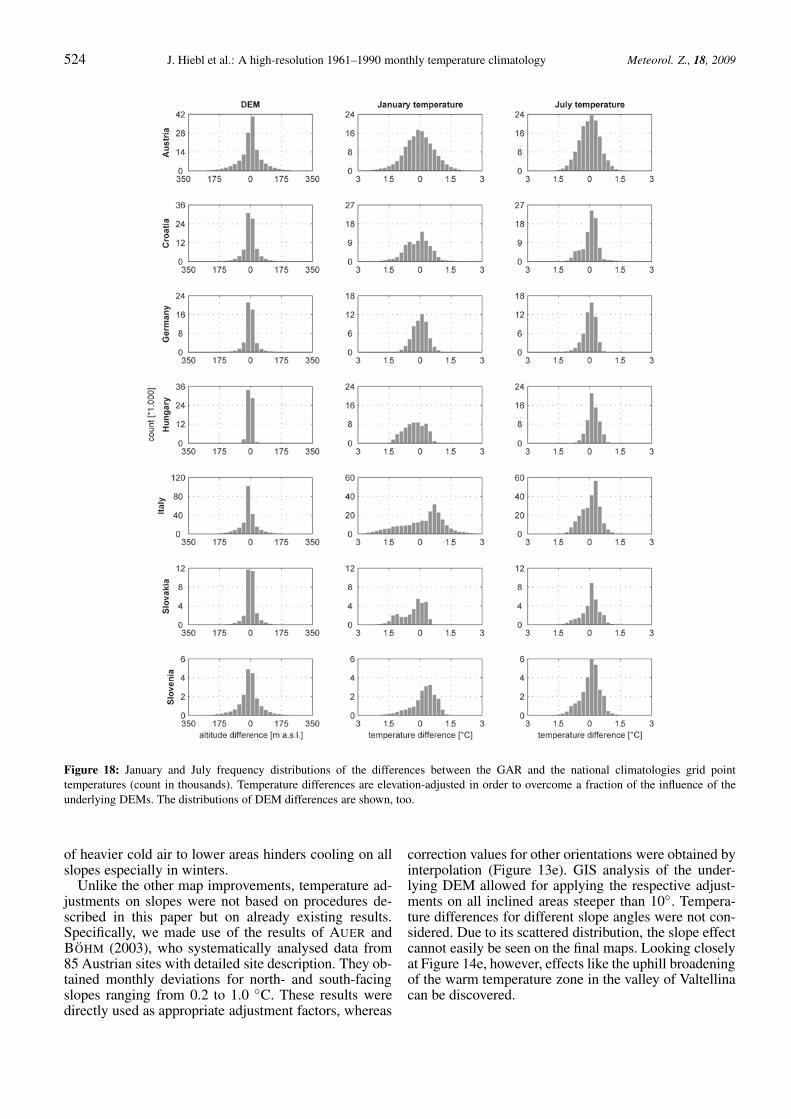
Figure 18: January and July frequency distributions of the differences between the GAR and the national climatologies grid pointtemperatures (count in thousands). Temperature differences are elevation-adjusted in order to overcome a fraction of the influence of theunderlying DEMs. The distributions of DEM differences are shown, too.
of heavier cold air to lower areas hinders cooling on allslopes especially in winters.
Unlike the other map improvements, temperature ad-justments on slopes were not based on procedures de-scribed in this paper but on already existing results.Specifically, we made use of the results of AUER andBOHM (2003), who systematically analysed data from85 Austrian sites with detailed site description. They ob-tained monthly deviations for north- and south-facingslopes ranging from 0.2 to 1.0 ◦C. These results weredirectly used as appropriate adjustment factors, whereas
correction values for other orientations were obtained byinterpolation (Figure 13e). GIS analysis of the under-lying DEM allowed for applying the respective adjust-ments on all inclined areas steeper than 10◦. Tempera-ture differences for different slope angles were not con-sidered. Due to its scattered distribution, the slope effectcannot easily be seen on the final maps. Looking closelyat Figure 14e, however, effects like the uphill broadeningof the warm temperature zone in the valley of Valtellinacan be discovered.
eschweizerbartxxx ingenta
Meteorol. Z., 18, 2009 J. Hiebl et al.: A high-resolution 1961–1990 monthly temperature climatology 525
3.6 Uncertainties
The accuracy of the temperature fields was assessed bymeans of the standard deviation of the station residu-als (hence referred to as standard error), which wereobtained as the differences between observed and mod-elled temperatures at the station locations. An alterna-tive approach could consist in comparing the pixel val-ues from the final gridded fields to the initial station dataat the respective coordinates (e.g. VAN DER SCHRIERet al., 2007). Such an evaluation procedure, however,suffers from the different spatial scale of the data tobe compared – gridded data with distinct pixel size onthe one hand and irregularly distributed point data onthe other hand. In particular, estimated differences fromsuch comparison can be strongly related to the differ-ences in elevation between the stations and the respec-tive pixel values.
As a precondition in terms of temperature field accu-racy, a maximum allowable standard error of 1 ◦C wasdetermined. In the following, the reduction of errors ob-tained by the main working steps of Chapters 3.1–3.5will be discussed (Figures 16 and 17):
– The standard errors of the linear temperature-elevationregressions over the whole GAR dataset ranged from1.25 ◦C in May to 2.27 ◦C in January; the corre-sponding average monthly error was 1.69 ◦C.
– An important improvement could be achieved throughregionalisation. Performing the simple regressionagainst elevation in seven different subregions de-creased the monthly errors to values ranging from0.81 ◦C in June to 1.39 ◦C in January, whereas theaverage monthly error was 1.02 ◦C.
– By considering, besides elevation, also longitude, lat-itude and distance from the coast in a multilinear re-gression the average monthly standard error was re-duced to 0.79 ◦C ranging from 0.66 ◦C in May to1.07 ◦C in December. The refinement of the region-alisation induced by the insertion of a third verticallayer did neither improve nor deteriorate the modelsignificantly in terms of the standard error. This re-finement is, however, important, as multilinear re-gressions could yield unreliable results if the depen-dent variable (temperature) and the most importantindependent variable (elevation) were not normallydistributed. Using different vertical layers consider-ably minimises the non-normal distribution issue.
– As far as additional improvements are considered,the reduction of the standard error is not the mostappropriate performance measure, because these im-provements hardly have any area-wide effect but areregionally or locally confined. Even so, the standarderror could once more be reduced: The final averagemonthly standard error was assessed with 0.69 ◦Cand it ranged between 0.62 ◦C in May and 0.85 ◦Cin December. The additional improvement, which
proved the most effective in terms of standard er-ror reduction, was the one corresponding to cold airpools, followed by the ones related to coastal beltsand urban areas. Lakeshore and slope adjustmentsdid not considerably alter the error, a fact which canbe traced back to the small number of concerned sta-tions and to the size of corrections.
Actually, in the discussion of the temperature fields’errors, some additional aspects have to be mentioned:(i) The first point concerns the errors induced by theDEM. Since altitude is the most important independentvariable in the regression models, every inaccuracy inthe DEM is directly transferred into a temperature error.GTOPO30 contains a root mean square error of about18 m (USGS, 1996). Given the different monthly andsubregional lapse rates, such DEM inaccuracy accountsfor a temperature error of 0.09 ◦C on average over thewhole GAR (minimum 0.06 ◦C in December, maximum0.11 ◦C in June). (ii) The second point concerns the er-rors in the temperature station data and their spatial rep-resentativity: It was our clear intention not to aim for afinal error of 0 ◦C. Aiming for an error smaller than 1 ◦Cwould ignore the fact that the remaining standard erroris only partly due to modelling shortcomings. In fact, anindefinable but potentially large fraction of the remain-ing error is due to inhomogeneities in the station data(temporal inhomogeneities could largely not be consid-ered here, see Chapter 2.2) and local peculiarities of thestation data in non-neutral surrounding. Allowing for afinal standard error was, therefore, necessary becausestation data always contains final measurement uncer-tainties and locally limited climate information.
So, the final standard errors were considered satisfac-tory and, even though to a certain extent they probablystill reflect uncaptured or wrongly captured climatologi-cal effects, we did not apply any further method for cor-recting the climatologies, e.g. by interpolating the resid-uals: In our opinion such a further reduction of the errorswould lack physical justification.
4 Comparison to national temperaturefields
Whereas the performance of the spatial modelling ap-proach by means of statistical measures was discussedin Chapter 3.6, we now want to compare the GAR tem-perature climatology to other existing gridded fields of1961–1990 normal temperatures. Comparisons amongdifferent temperature fields can only show differencesbetween the models, but they can neither validate themnor estimate any modelling success. Whereas computeddifferences between the results cannot be used to deriveany order of modelling successes, they can, however, beused to quantify the uncertainty of spatial modelling ofclimate fields. EFTHYMIADIS et al. (2006) and FREI andSCHAR (1998) used such comparison to show their spa-tial modelling results in the light of other gridded fieldsfor the same region.
eschweizerbartxxx ingenta
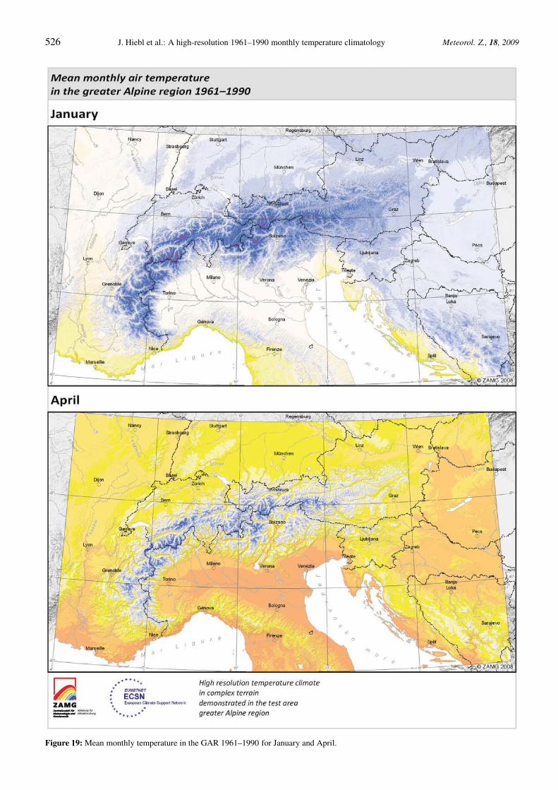
526 J. Hiebl et al.: A high-resolution 1961–1990 monthly temperature climatology Meteorol. Z., 18, 2009
Figure 19: Mean monthly temperature in the GAR 1961–1990 for January and April.
eschweizerbartxxx ingenta
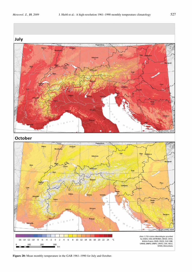
Meteorol. Z., 18, 2009 J. Hiebl et al.: A high-resolution 1961–1990 monthly temperature climatology 527
Figure 20: Mean monthly temperature in the GAR 1961–1990 for July and October.
eschweizerbartxxx ingenta
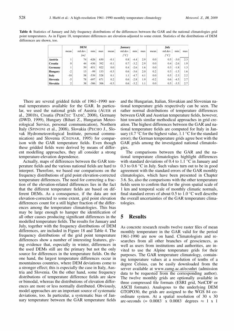
528 J. Hiebl et al.: A high-resolution 1961–1990 monthly temperature climatology Meteorol. Z., 18, 2009
Table 4: Statistics of January and July frequency distributions of the differences between the GAR and the national climatologies gridpoint temperatures. As in Figure 18, temperature differences are elevation-adjusted to some extent. Statistics of the distributions of DEMdifferences are shown, too.
DEM January July mean std.dev. min max mean std.dev. min max mean std.dev. min max
[m] [°C] [°C]
Austria 1 74 -626 630 -0.1 0.8 -4.4 2.9 0.0 0.5 -3.0 2.3
Croatia 0 44 -436 392 -0.1 0.7 -3.2 2.9 0.0 0.4 -2.6 1.9
Germany 1 59 -851 922 0.0 0.4 -2.6 1.6 0.0 0.3 -1.8 1.3
Hungary -2 13 -99 133 -0.3 0.6 -3.6 2.0 0.2 0.3 -1.5 1.6
Italy -10 58 -539 528 0.1 1.1 -4.7 4.1 0.0 0.5 -2.3 2.2
Slovenia -5 78 -697 671 0.2 0.6 -2.8 1.9 -0.2 0.6 -4.5 2.7
Slovakia 2 38 -386 306 -0.3 0.6 -3.2 1.1 0.0 0.5 -3.5 2.7
There are several gridded fields of 1961–1990 nor-mal temperatures available for the GAR. In particu-lar, we used the national grids of Austria (AUER etal., 2001b), Croatia (PERCEC TADIC, 2008), Germany(DWD, 1999), Hungary (Bihari Z., Hungarian Meteo-rological Service, personal communication), NorthernItaly (SPINONI et al., 2008), Slovakia (PECHO J., Slo-vak Hydrometeorological Institute, personal commu-nication) and Slovenia (CEGNAR, 1995) for compar-ison with the GAR temperature fields. Even thoughthese gridded fields were derived by means of differ-ent modelling approaches, they all consider a strongtemperature-elevation dependence.
Actually, maps of differences between the GAR tem-perature fields and the various national fields are hard tointerpret. Therefore, we based our comparisons on thefrequency distributions of grid point elevation-correctedtemperature differences. The need for correcting a frac-tion of the elevation-related differences lies in the factthat the different temperature fields are based on dif-ferent DEMs. As a consequence, if the data are notelevation-corrected to some extent, grid point elevationdifferences count for a still higher fraction of the differ-ences among the temperature climatologies. This biasmay be large enough to hamper the identification ofall other causes producing significant differences in themodelled temperature fields. The results for January andJuly, together with the frequency distributions of DEMdifferences, are included in Figure 18 and Table 4. Thefrequency distributions of the grid point temperaturedifferences show a number of interesting features, giv-ing evidence that, especially in winter, differences inthe used DEMs still are the primary but not the onlysource for differences in the temperature fields. On theone hand, the largest temperature differences occur inmountainous countries, where DEM deviations come toa stronger effect; this is especially the case in Italy, Aus-tria and Slovenia. On the other hand, some frequencydistributions of temperature difference fields are skewor bimodal, whereas the distributions of elevation differ-ences are more or less normally distributed. Obviously,model approaches are an important source of systematicdeviations, too. In particular, a systematic bias of Jan-uary temperature between the GAR temperature fields
and the Hungarian, Italian, Slovakian and Slovenian na-tional temperature grids respectively can be seen. Therather normal distributions of temperature differencesbetween GAR and Austrian temperature fields, however,hint towards similar methodical approaches in grid cre-ation. The highest differences between the GAR and na-tional temperature fields are computed for Italy in Jan-uary (4.7 ◦C for the highest value, 1.1 ◦C for the standarderror); the German temperature grids agree best with theGAR grids among the investigated national climatolo-gies.
The comparisons between the GAR and the na-tional temperature climatologies highlight differenceswith standard deviations of 0.4 to 1.1 ◦C in January and0.3 to 0.6 ◦C in July. Such values turn out to be in goodagreement with the standard errors of the GAR monthlyclimatologies, which have been presented in Chapter3.6. So, also the comparisons with the other temperaturefields seem to confirm that for the given spatial scale of1 km and temporal scale of monthly climatic normals,final standard errors of about 0.5 to 1.0 ◦C well describethe overall uncertainties of the GAR temperature clima-tologies.
5 Results
As concrete research results twelve raster files of meanmonthly temperature in the GAR valid for the period1961-1990 are now on hand. Climatologists and re-searches from all other branches of geosciences, aswell as users from institutions and authorities, are in-vited to use the Alpine temperature grids for theirpurposes. The GAR temperature climatology, contain-ing temperature values at a resolution of tenths of adegree Celsius, can be easily downloaded from theserver available at www.zamg.ac.at/ecsnhrt (admissiondata to be requested from the corresponding author).The twelve monthly grids are optionally available inthree compressed file formats (ESRI grid, NetCDF orASCII formats). Analogous to the underlying DEMGTOPO30, the grids are assigned to the WGS 84 co-ordinate system. At a spatial resolution of 30 x 30arc-seconds (= 0.0083· x 0.0083· degrees ≈ 1 x 1
eschweizerbartxxx ingenta
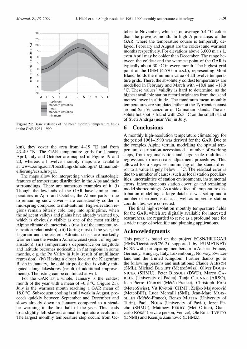
Meteorol. Z., 18, 2009 J. Hiebl et al.: A high-resolution 1961–1990 monthly temperature climatology 529
maximum
standard deviation
mean
standard deviation
minimum
Figure 21: Basic statistics of the mean monthly temperature fieldsin the GAR 1961–1990.
km), they cover the area from 4–19 ◦E and from43–49 ◦N. The GAR temperature grids for January,April, July and October are mapped in Figure 19 and20, whereas all twelve monthly maps are availableat www.zamg.ac.at/forschung/klimatologie/ klimamod-ellierung/ecsn hrt-gar.
The maps allow for interpreting various climatologicfeatures of temperature distribution in the Alps and theirsurroundings. There are numerous examples of it: (i)Though the lowlands of the GAR have similar tem-peratures in April and October, the Alpine parts – dueto remaining snow cover – are considerably colder inmid-spring compared to mid-autumn. High-elevation re-gions remain bitterly cold long into springtime, whenthe adjacent valleys and plains have already warmed up,which is obviously visible as one of the most strikingAlpine climate characteristics (result of the temperature-elevation-relationship). (ii) During most of the year, theLigurian and the eastern Adriatic coasts are markedlywarmer than the western Adriatic coast (result of region-alisation). (iii) Temperature’s dependence on longitudeand latitude becomes noticeable in flat regions in somemonths, e.g. the Po Valley in July (result of multilinearregression). (iv) Having a closer look at the KlagenfurtBasin in January, the cold air pool effect is visibly mit-igated along lakeshores (result of additional improve-ments). The listing can be continued at will.
For the GAR as a whole, January is the coldestmonth of the year with a mean of –0.8 ◦C (Figure 21).July is the warmest month reaching a GAR mean of18.0 ◦C. Subsequent cooling is still weak in August, pro-ceeds quickly between September and December andslows already down in January compared to a stead-ier warming in the first half of the year. This leadsto a slightly left-skewed annual temperature evolution.The largest monthly temperature step occurs from Oc-
tober to November, which is on average 5.4 ◦C colderthan the previous month. In high Alpine areas of theGAR, where the temperature course is temporally de-layed, February and August are the coldest and warmestmonths respectively. For elevations above 3,000 m a.s.l.,even April may be colder than December. The range be-tween the coldest and the warmest point of the GAR istypically about 30 ◦C in every month. The highest gridpoint of the DEM (4,570 m a.s.l.), representing MontBlanc, holds the minimum value of all twelve tempera-ture grids. There, the absolutely coldest temperatures aremodelled in February and March with –18.8 and –18.9◦C. These values’ validity is hard to determine, as thehighest available station record originates from thousandmetres lower in altitude. The maximum mean monthlytemperatures are simulated either at the Tyrrhenian coastaround San Vincenzo or on Dalmatian islands. The ab-solute hot spot is found with 25.3 ◦C on the small islandof Sveti Andrija (near Vis) in July.
6 ConclusionsA monthly high-resolution temperature climatology forthe period 1961–1990 was derived for the GAR. Due tothe complex Alpine terrain, modelling the spatial tem-perature distribution necessitated a number of workingsteps, from regionalisation and large-scale multilinearregressions to mesoscale adjustment procedures. Thisallowed for a stepwise minimising of the standard er-ror to a value largely below 1 ◦C. The residual error isdue to a number of causes, such as local station peculiar-ities, uncertainties of station environments, instrumentalerrors, inhomogeneous station coverage and remainingmodel shortcomings. As a side effect of temperature dis-tribution modelling, a large database was set up and anumber of erroneous data, as well as imprecise stationcoordinates, were corrected.
The final high-resolution monthly temperature fieldsfor the GAR, which are digitally available for interestedresearchers, are regarded to serve as a profound base fora wide range of scientific and planning applications.
AcknowledgmentsThis paper is based on the project ECSN/HRT-GAR(EMN/Decisions/C26-2) supported by EUMETNET/ECSN with participating members from Austria, France,Germany, Hungary, Italy, Luxembourg, Norway, Switzer-land and the United Kingdom. Further thanks go tothe following persons and institutions: Claude ALESCH(SML), Michael BEGERT (MeteoSwiss), Oliver BOCH-NICEK (SHMU), Peter BISSOLI (DWD), Marco CA-REER (University of Padua), Tanja CEGNAR (ARSO),Jean-Pierre CERON (Meteo-France), Christoph FREI
(MeteoSwiss), Vıt Kveton (CHMI), Zeljko Majstorovic(MeteoBiH), Luca Mercalli (SMI), Jean-Marc MOIS-SELIN (Meteo-France), Renzo MOTTA (University ofTurin), Paola NOLA (University of Pavia), Jozef Pe-cho (SHMU), Matthew PERRY (Met Office), Gian-carlo ROSSI (private person, Venice), Ole Einar TVEITO(DNMI) and Ksenija Zaninovic (DHMZ).
eschweizerbartxxx ingenta
530 J. Hiebl et al.: A high-resolution 1961–1990 monthly temperature climatology Meteorol. Z., 18, 2009
ReferencesAUER, I., R. BOHM, 2003: Jahresmittel der Lufttemperatur.
– In: Bundesministerium fur Land- und Forstwirtschaft,Umwelt und Wasserwirtschaft (Ed.): Hydrologischer AtlasOsterreichs. – Osterreichischer Kunst- und Kulturverlag,Vienna, Map Sheet 1.6.
AUER I., R. BOHM, H. MOHNL, 1989: Klima von Wien:eine anwendungsorientierte Klimatographie. – Magistratder Stadt Wien, Vienna, 270 pp.
AUER, I., R. BOHM, W. SCHONER, 2001a: Austrianlong-term climate 1767-2000: multiple instrumental cli-mate time series from Central Europe. – OsterreichischeBeitrage zu Meteorologie und Geophysik 25, 147 pp., plusCD-ROM.
AUER, I., R. BOHM, H. MOHNL, R. POTZMANN, W.SCHONER, P. SKOMOROWSKI, 2001b: OKLIM: digitalerKlimaatlas Osterreichs. – Zentralanstalt fur Meteorologieund Geodynamik, Vienna, CD-ROM.
BELLARDONE G., A. BIANCOTTI, S. BOVO, L. MOTTA, B.CAGNAZZI, 1998: Precipitazioni e temperature. – RegionePiemonte, Universita degli Studi di Torino, Dipartimento discienze della Terra, Turin, CD-ROM.
BRUNETTI, M., G. LENTINI, M. MAUGERI, T. NANNI, C.SIMOLO, J. SPINONI, 2009: Estimating local records forNorthern and Central Italy from a sparse secular temper-ature network and from 1961-1990 climatologies. – Adv.Sci. Res. 3, 63–71.
BOHM, R., 1998: Urban bias in temperature time series:a case study for the city of Vienna, Austria. – ClimaticChange 38, 113–128.
CEGNAR, T. (Ed.), 1995: Climate of Slovenia. – Hydromete-orological Institute of Slovenia, Ljubljana, 70 pp.
DALY, C., 2006: Guidelines for assessing the suitability ofspatial climate data sets – Int. J. Climatol. 26, 707–721.
DALY, C., W.P. GIBSON, G.H. TAYLOR, G.L. JOHNSON,P.A. PASTERIS, 2002. A knowledge-based approach to thestatistical mapping of climate. – Climate Res. 22, 99–113.
DALY, C., M. HALBLEIB, J.I. SMITH, W.P. GIBSON, M.K.DOGGETT, G.H. TAYLOR, J. CURTIS, P.A. PASTERIS,2008: Physiographically-sensitive mapping of temperatureand precipitation across the conterminous United States. –Int. J. Climatol. 28, 2031–2064, DOI: 10.1002/joc.1688.
DWD (Deutscher Wetterdienst), 1999: Klimaatlas Bundesre-publik Deutschland: Teil 1. – DWD, Offenbach, CD-ROM.
EFTHYMIADIS, D., P.D. JONES, K.R. BRIFFA, I. AUER,R. BOHM, W. SCHONER, C. FREI, J. SCHMIDLI, 2006:Construction of a 10-min-gridded precipitation data set forthe greater Alpine region for 1800-2003. – J. Geophys. Res.111, D01105, DOI: 10.1029/2005JD006120.
ENDERS, G. (Ed.), 1996: Klimaatlas von Bayern. – Bay-erischer Klimaforschungsverbund, Munich, 105 pp.
FREI, C., C. SCHAR, 1998: A precipitation climatology ofthe Alps from high-resolution rain gauge observations. –Int. J. Climatol. 18, 873–900.
KAMTZ, F.L., 1860: Uber die Ableitung mittlerer Resultateaus meteorologischen Beobachtungen. – Repertitorium furMeteorologie 1, 107–134.
KIRCHHOFER, W. (Ed.), 1982: Klimaatlas der Schweiz. –Schweizerische Meteorologische Anstalt, Bundesamt furLandestopographie, Wabern-Bern.
LUBW (Landesanstalt fur Umwelt, Messungen undNaturschutz Baden-Wurttemberg), 2006: KlimaatlasBaden-Wurttemberg. – LUBW, Karlsruhe – CD-ROM.
MERCALLI, L. (Ed.), 2003: Atlante climatico della Valled’Aosta. – Societa Meteorologica Subalpina, Turin, 416 pp.
METEO-FRANCE, Direction de la Climatologie, 1999: Leclimat de la France. – Meteo-France, Toulouse, CD-ROM.
METEO-FRANCE, Direction de la Climatologie, 2004: Cli-mate atlas of Europe. – Meteo-France, Toulouse, CD-ROM.
MUCHER S., K. STEINNOCHER, J.L. CHAMPEAUX, S.GRIGUOLO, K. WESTER, C. HEUNKS, V. VAN KATWIJK,2000: Establishment of a 1-km pan-European land coverdatabase for environmental monitoring. – IAPRS 33, 702–709.
NCDC (National Climatic Data Center), 1998: WMO 1961–1990 global climate normals. – NCDC, Asheville – CD-ROM.
PERCEC TADIC, M., 2008: Geostatistical mapping of cli-matological variables. – In: ZANINOVIC K., M. GAJIC-CAPKA, M. PERCEC TADIC: Klimatski atlas Hrvatske: cli-mate atlas of Croatia 1961–1990, 1971–2000. – Meteoro-logical and Hydrological Service of Croatia, Zagreb, 200pp.
SCHWARB, M., 2000: The Alpine precipitation climate: eval-uation of a high-resolution analysis scheme using compre-hensive rain-gauge data. – Swiss Federal Institute of Tech-nology (ETH), Zurich, Switzerland, 131 pp. (PhD thesis13911).
SPINONI, J., M. BRUNETTI, G. LENTINI, M. MAUGERI,T. NANNI, 2008: Construction of 1961–90 high-resolutionmonthly temperature climatologies for Northern Italy. – In:AUER I., R. BOHM, J. HIEBL, W. SCHONER, J. SPINONI,G. LENTINI, M. MAUGERI, M. BRUNETTI, T. NANNI,M. PERCEC TADIC, Z. BIHARI: ECSN-HRT/GAR: highresolution temperature climatology in complex terrain –demonstrated in the test area greater Alpine region GAR.– Central Institute for Meteorology and Geodynamics, Vi-enna, Annex 3.
STEINHAUSER, F. (Ed.), 1970: Climatic atlas of Europe I:maps of mean temperature and precipitation. – WMO,UNESCO, Geneva.
TOLASZ, R., R. BRAZDIL, O. BULIR, P. DOBROVOLNY,M. DUBROVSKY, L. HAJKOVA, O. HALASOVA, J.HOSTYNEK, M. JANOUCH, M. KOHUT, K. KRSKA,S. KRIVANCOVA, V. KVETON, Z. LEPKA, P. LIP-INA, J. MACKOVA, L. METELKA, T.MIKOVA, Z.MRKVICA, M. MOZNY, J. NEKOVAR, L. NEMEC, J.POKORNY, J.D. REITSCHLAGER, D. RICHTERNOVA, J.ROZNOVSKY, M. REPKA, D. SEMERADOVA, V. SOSNA,M. STRIZ, P. SERCI, H. SKACHOVA, P. STEPANEK,P. STEPANKOVA, M. TRNKA, A. VALERIANOVA, J.VALTER, K. VANICEK, F. VAVRUSKA, V. VOZENILEK,T. VRABLIK, M. VYSOUDIL, J. ZAHRADNICEK, I.ZUSKOVA, M. ZAK, Z. ZALUD, 2007: Atlas PodnebiCeska: Climate atlas of Czechia. – Czech Hydrometeoro-logical Institute, Prague, 254 pp.
USGS (United States Geological Sur-vey), 1996: GTOPO30 Documentation –http://edc.usgs.gov/products/elevation/gtopo30/README.html.
VAN DER SCHRIER, G., D. EFTHYMIADIS, K.R. BRIFFA,P.D. JONES, 2007: European Alpine moisture variabil-ity for 1800-2003. – Int. J. Climatol. 27, 415–427, DOI:10.1002/joc.1411.
eschweizerbartxxx ingenta