OPERATIONS RESEARCHVERFAHRENMETHODSOFOPERATIONS RESEARCH

35

Herausgeber - Editorial Board RUDOLF HENN, KARLSRUHEPETER KALL, ZÜRICHHEINZ KONIG, SAARBRÜCKENBERNHARD KORTE, BONNOLAF KRAFFT, AACHENKLAUS NEUMANN, KARLSRUHEWERNER OETTLI, MANNHEIM

.. KLAUS RITTER, STUTTGART)OACHIM ROSENMÜLLER, BIELEFELDNORBERT SCHMITZ, MÜNSTERHORST SCHUBERT, DÜSSELDORF

Sonderdruck W ALTER VOGEL, BONN

III SYMPOSIUM ON OPERATIONS RESEARCHU niversitât Mannheim, September 6-8, 1978Tagungsbericht - Proceedings.

Herausgegeben von:Edited by:

In Zusammenarbeit mit..In Cooperation with: '

Sektion 5: 'Anwendungen - 'Applications

WERNER OETTLI, MANNHEIM, FRANZ STEFFENS, MANNHEIM

HERMANN GOPPL, KARLSRUHE. PETER KALL, ZÜRICH ,BERNHARD KORTE, BONNWERNER KRABS, DARMSTADT

.' ,

OTTO MOESCHLIN, HAGEN, BURKARD RAUHUT, AACHEN

VerlagsgruppeATHENÀ UM / HAIN / SCRIPTOR / HANSTEIN

A Heuristic Algorithm for the Locationand Dimensioning of Warehouses

Cesar D. B. Monterosso and Claudio Thomas Bornstein, Rio de Janeiro')

ABSTRACT: A heuristic algorithm is presented for locatingand dimensioning warehouses which is sufficiently flexibleto incorporate the variability and particularities ofdeveloping countries, including capacity constraints.

The goal is to minimize warehousing andtransportation costs. To attain this objective we use anout-of-kilter algorithm determining the flow with minimumtotal cost. As we consider economies of scale, unit costsat each arc are a function of the flows, i.e. the problemis actually non-linear. To establish the values of unitcosts we use an iterative procedure.

The method converges but not necessarily to aglobal optimum, so that a sub-routine called OROP is usedas a second part of the heuristic procedure.

I. INTROOUCTION

The problem is defined as follows: given afinite set of production centers, demand centers andcandidate warehouse sites, locate and dimension warehousesso as to minimize total transportation and warehousingcosts.

The algorithm is tested for several problemsbased on data from the Brazilian Storage Company (CIBRA-ZEM) for rice in Maranhão, a state in north Brazil.

Some of the ideasdeveloped here build on workdone by FELOMAN, LEHRER and RAY 131, KUEHN and HAMBURr,ER

'l COPPE/UFRJ, Programa de Engenharia de Sistemas, Caixa Postal 1191, 20.000 - Rio deJaneiro - RJ Brazil

316

161. KING and LOGAN 171.

11. A MATHEMATICAL MODEL

Consider a single product. with given supliesand demands for each production and consumer center. Thewarehouses should store all production and meet alldemands. for a period long enough to include the relevantseasonal variations, At the end of the period. we assumethat the same seasonal variations will happen again in thefollowing period. Thus. the problem is static. For eachperiod total production is equal to total demandoFictitious warehouses. production or consumer centersmay be introduced io order to meet these conditions.,

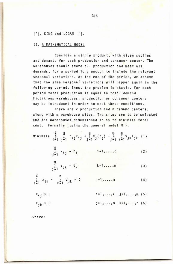
There are i production and n demand centers.along with m warehouse sites. The sites are tõ be selectedand the warehouses dimensioned 50 as to minimize totalc o s t . Formally (usíng the general model M 1 ) :

i m m TTi nMinimize 'i I rijxij + L C.(t.) + r Is·kZ·k (1 )

i = 1 j = 1 j = 1 J J j = 1 k = 1 J J

mI xij Pi i =1 •...• i (2)j = 1mL Zj k dk k=l •...• n (3 )j = 1

i nI x .. - L Z j k o j =1 •...• m (4 )

i= 1 lJ k=l

xij > o i = 1 •...• i j=l •... ,m ( 5 )

Zj k > o j=l •...• m k=l, ...• n (6 )

where:

1---I

317

Flow from production center to warehouse j

Pi Production at center

Zjk Flow from warehouse j to demand center k

dk Demand at center k

rij Unit transportation cost from production center

to warehouse j

Sjk Unit transportation cost from warehouse j to demand

center k ..t

t , I x.· = Throughput or flow through warehouse jJ i=l 1J

Cj(tj) = Warehousing cost function for warehouse j.Warehousing costs vary essential1y with the

static capacity. Since static capacity is a function of

the throughput, the relation is included in the Cj(tj) termo

Since there are economies of scale, the function

Cj(tj) is concave and the model Ml is nonlinear. CANDLER,

SNYDER and FAUGHT 111 use concave programming for such

cost functions.Cj(tj) can also be approximated by a piecewice

1 i nea r funct ion (see fi gure 1), sol vab l e by mi xed i nteger

programming. GEOFFRION and GRAX~S 151, SWEENEY and TATHAM

191 use Benders Decomposition to solve this problem.

'//

//

/

'I

Figure 1

318

In this paper we develop an iterative procedure.At each iteration k , the values of the unit warehousingcosts c~ are fixed. Thus, the warehousing cost function

J k k kmay be represented by cj . tj, where cj is constant foreach iteration k. However, th e unit warehousing costs area function gj(tj) of the flows tj. We say that at iterationk we reach a state of equilibrium for a warehouse j if

k kcj = gj(tj).

As we show in the next section, the first part ofthe heuristic method (called the EQUILIBRATE routine) findsa solution where a state of equilibrium is reached for eachwarehouse j. This solution is called an equilibriumsolution.

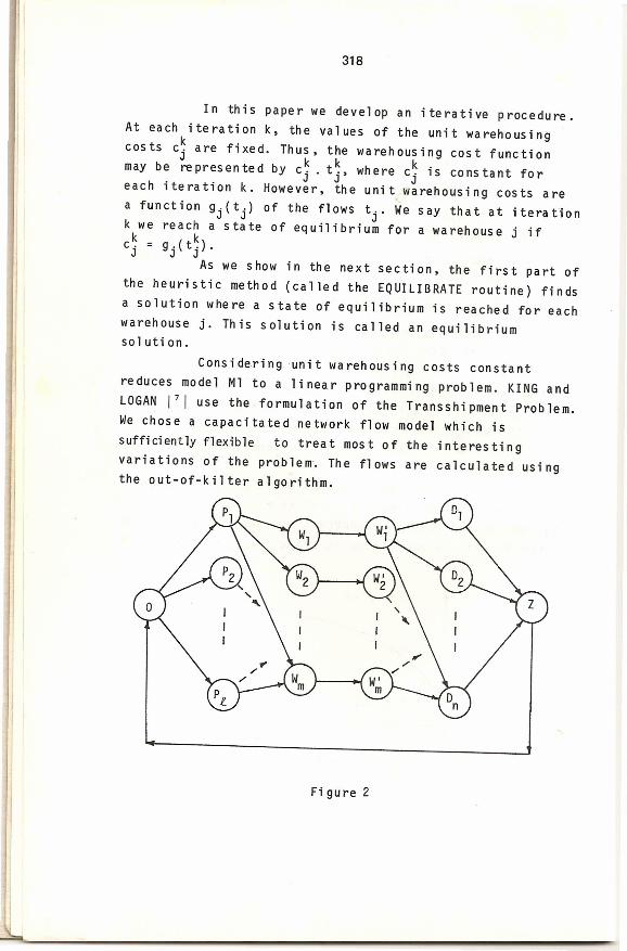
Consideringunit warehousing costs constantreduces model Ml to a linear programming problem. KING andLOGAN /7/ use the formulation of the Transshipment Problem.We chose a capacitated network flow model which issufficiently flexible to treat most of the interestingvariations of the problem. The flows are calculated usingthe out-of-kilter algorithm.

Figure 2

319

A graphical illustration of the problem is given infigure 2 where Pi, Wi and Di are nodes representingproduction centers, warehouses and demand centerso Eachwarehouse j 1s represented by an arc (Wo,W~)o Arcs (O,P.)

J J 1and (Di'Z) represent the production and the demand atcenter Pi and Di respectivelyo The arc leading from Z toO merely transforms the network into a circulation (networkwithout sources and sinks) o Th í s permits the useof the out-of-kilter algorithm to calculate the flow withminimum costo To each arc(i~j) we associate threeparameters aij, bij and cij representing respectively thelower and upper bounds on the flow and the unit costo

We wtll use the following notation:set of all nodes of the networkset of all arcs of the network

N

APW

D

{(O,P1 )ooo,(O,Pt)}{(Wl,Wi),ooo,(Wm'W~)}{(Dl ,Z), o o o, (Dn ,Z)

wi th:andandtI p.

j = 1 J

O for (i ,j ) e: P

O for (i ,j ) e: Dn1- d. and cz,O = O o

i= 1 1

For the other arcs aij and bij denoterespectively the minimum and maximum capacity of a routeor a warehouseo cij represents the unit transportationor warehousing cost depending on the nature of arc(i ,j)o

By setting appropriate values to aij,bij andc .. we may c o n sid e r many particular cendit ions . By

lJallowing several arcs to join the same pair of nodes, wemay represent the case where several means oftransportation exist as well as the case where thewarehouses are composed of modulated unitso

We may now formulate the model M2 correspondingto the capacitated network flowo

320

Minimize I Cij xij (7)(i.j)€A

I x .. - L xji o V e N (8 )lJj€r+( i) j€r (i )aij .::xij .::bij V (i ,j)€ A (9)

where x .. is the flow at the arc (.i.j).r+(i) and r-ti) arelJrespectively the setof nodes following and preceding nodei.

As said. the model M2 assumes constant unitcosts cij for each arc(i.j). This is of course not true ifwe consider economies of scale. In the next section wewill present the heuristic procedure and the EQUILIBRATEroutine which solves this problem.

111. SOLUTION METHOD

In the previous section we saw how the generalmodel Ml may be reduced to a simpler one (model M2).wherewe have constant unit warehousing costs. As we considereconomies of scale. unit warehousing costs actuallydecrease as flows increase.

For model M2 we use the out-of-kilter algorithmdetermining flows xij for each arc(i.j) 50 as to minimizetotal cost. We will show how to use the EQUILIBRATEroutine trying to reach a state df equilibrium for eacharc(i.j) € W.

kLet cij be the unit warehousing cost forarc(i.j) € W at iteration k. For the other arcs the unitcosts remain constant through all iterations and are equalto zero or correspond to unit transportation costs. X~j isthe flow for arc(i,j) at iteration k. The EQUILIBRATEroutine consists of the following steps:STEP O: k:=O

Assign the smallest possible value to C~j for all

321

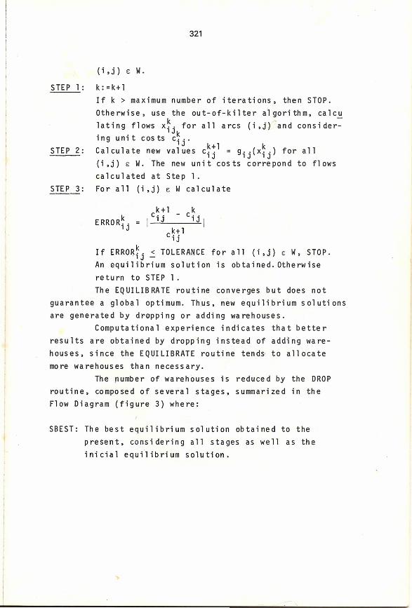
STEP 1:

(i,j)EW.

k:=k+l

If k > maximum number of iterations, then STOP.

Otherwise, use the out-of-kilter algorithm, calcu

lating flows X~j for all arcs (i ,j) 'and consi der-=-

ing unit costs c~ ..lJ k+l k

Calculate new values cij = gij(xij) for all

(i,j) E W. The new unit costs correpond to flows

ca 1cul ated at Step 1.

For all (i,j) E W calculate

STEP 2:

S TE P 3:

kERRORij

k + 1c· .I lJc~-I:l

1 J

If ERROR~j < TOLERANCE f o r a 11 (i, j) E W, STOP .

An equilibrium solution is obtained.Otherwise

return to STEP 1.

The EQUILIBRATE routine converges but does not

guarantee a global optimum. Thus, new eq.uilibrium solutions

are generated by dropping or adding warehouses.

Computational experience indicates that better

results are obtained by dropping instead of adding ware-

houses, since the EQUILIBRATE routine tends to allocate

more warehouses than necessary.

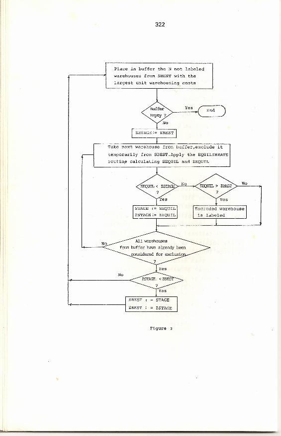
The number o f warehouses is reduced by the DROP

routine, composed of several stages, summarized in the

Flow Diagram (figure 3) where:

SBEST: The best equilibrium solution obtained to the

present, considering all stages as we11 as the

inicial equilibrium solution.

322

Place in buffer the N not labeledwarehouses frorn SBEST with thelargest unit warehousing costs

BufferErrpty?

No

)- y_e_~

~TAGE:= ZBeZTJI

Take next warehouse from buffer,exclüde it

ternporarily frorn SBEST.Apply the EQUILIBRATEroutin~ calculating SEQUIL and ZEQUIL

?

ZEQUIL< ZSTAGE:>--,N~O'é..--><ZEQUIL > ZBEST?

Figure 3

323

STAGE: The best equilibrium solution at a certain stageof the DROP routine.

SEQUIL:An equilibrium solution obtained by the EQUILIBRATEroutine.

ZBEST,ZEQUIL,ZSTAGE: Total cost relating to SBEST,SEQUILand STAGE respectively.

A stage is started by placing warehouses in thebuffer. One by one the warehouses of the buffer aretemporarily excluded from SBEST by assigning them a veryhigh unit cost. Let j be a warehouse from the buffer whichwill be excluded temporarily. Applying the EQUILIBRATEroutine we get a new solution SEQUIL. If ZEQUIL < ZSTAGEwe keep the new solution as the best in the stage. Then,we replace warehouse j in SBEST and choose a new warehousefor temporary exclusion.

If ZEQUIL ~ ZSTAGE but ZEQUIL ~ ZBEST ,replace warehouse j in SBEST and continue as in the caseabove, choosing a new warehouse for temporary exclusion.If however ZEQUIL ~ ZSTAGE and ZEQUIL > ZBEST, thenwarehouse j will be labeled. A labeled warehouse will nolonger be considered for exclusion in any further stage,i·.e., will not be placed in a buffer.

A stage ends when all the warehouses in thebuffer have already been temporarily excluded. At eachstage no more then one warehouse will be definitelyexcluded and this will only happen if ZSTAGE < ZBEST.

If a stage ends, new unlabeled warehouseswill be placed in the buffer, thus beginning a new stage.The DROP routine ends if no warehouse can be placed inthe buffer.

Clearly the more warehouses placed in thebuffer,the more likely are improved solutions at theexpense of more computational time.The size of the bufferis a parameter of the DROP routine and will depend on the

324

required quality of the solution.We may now describe the full heuristic proce-

dure. First an inicial equilibrium solution is generatedusing the EQUILIBRATE routine. Then we try to get a betterequilibrium solution by means of the OROP routine, i.e.,by dropping warehouses. The OROP routine uses theEQUILIBRATE routine to get new equilibrium solutions.When using the EQUILIBRATE routine the flows arecalculated by the out-of-kilter algorithm.

IV. RESULTSIn this section we illustrate the operation of

the EQUILIBRATE and the OROP routines,considering amicroregion in the state of Maranhão.

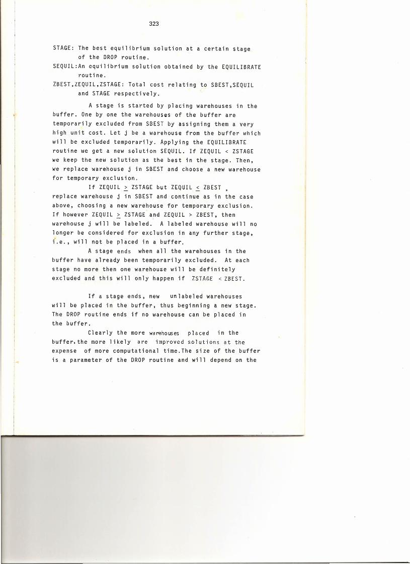
Table 1 shows how the EQUILIBRATE routine getsan equilibrium solution in three iterations.

The unit costs C~j are given in cruzeiros, X~jis given in tons and the tolerance is 0.002. Theexpression used to calculate unit costs as a function offlows was:

k8(xi/hij)

for (i,j)E W, where (X~j/hij) is the static capacit{,expressed as a function of the throughput or flow xijthrough the warehouse (i ,j).hij is a constant for eachwarehouse ti ,j).

As we see, the EQUILIBRATE routine convergesvery quickly. The second iteration almost yields anequilibrium between unit costs and flows and the thirdit e ra t io n p ro v ide s a n e q u il ib r ium sol u t io n . H a v in 9obtained the initial equilibrium solution,we use the OROProutine trying to get a better one. Table 2 illustratesthe operation of the OROP routine considering the samemicroregion of the example in Table 1.

. --~---~---------

Iteration 1 I Itera"tion 2 Iteration 3Location ° 1 1 rnl. 1 2' 2 rn2. 2 3 3 rn3.c .. xij c .. cij x .. cij c .. x .. cijl.J l.J l.J l.J l.J l.J l.J l.J

i !53,3121782 21782 IBOM JJ,RDIM 25,0 21782 53,3' 0,53 53,3 0,00 53,3 53,3 0,00

LGO. PEDRA 25,0 14872 56,9 0,56 56,9 14872 56,9 0,00 56,9 14872 56,9 0,00

MONÇÃO 25,0 39459 49,8 0,49 49,8139459 4'9,8 0,00 49,8 39459 49,8 0,00

PINDARE 25,0 ° 351,1 0,00 1351,11 ° 351,1 0,00 I 351,1 ° 351,1 0,00,~ 53,91 20:;'98

ISTA INEs 25,0 20198 53,9 0,53 53,9 0,00 53,9 20198 53,9 0,00 I

STA LUZIA 25,0 66000 48,1 0,48 48,1 66000 48,1 0,00 48,1 66000 48,1 0,00

VIT. FREIRE 25,0 30,801 51, ° 0,51 ",O aosoi I ",O 0,00 si .; I aosoi ",' 0,00BACABAL 25,0 43052 49,4 0,49 49'4149696 I 48,9 0,01 48,9 49696 48,9 0,00

IPIXUNA 25,0 6644 70,2 0,64 I 70,2 ° 1351,1 10,00 ! 351,1 ° 351,1 0,00

OLHO D'AGUA

I25,0 22747 52,8 0,52 sa.s I "''' ",' I0,00 I ",0 "''' I sz .e I 0,00

PEDREIRAS 25,0 12842 58,3 0,57 58,3112842 58,3 0,00 I1 58,3 12842 158,310,00

P. DE PEDRA 25,0 31748 50,7 0,50 .1 ;O" i "'" so ,» I 0,00 I' ;o,, "''' so .» I 0,00ST. A. LOPES 25,0 22214 52,9 0,52 ii 52,91 22214 52,910,00 I1 52,9 22214 52,9 0,00

Table 1

WN01

326

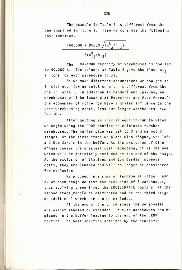
The example in Table 2 is different from theone examined in Table 1. Here we consider the followingcost function.

1500000 + 95000J(X~/hij)'k8(xi/hij)

The maximum capacity of warehouses is now setto 60.000 t. The columns at Table 2 give the flows xijin tons for each warehouse (i,j).

As we make different assumptions we now get aninicial equilibrium solution with is different from theone in Table 1. In addition to Pindare and Ipixuna, nowarehouses will be located at Pedreiras and P.de Pedra.Asthe economies of scale now have a grater influence on theunit warehousing costs, less but larger warehouses arelocated.

After getting an inicial equilibrium solutionwe begin using the DROP routine to eliminate furtherwarehouses. The buffer size was set to 3 and we got 3,stages. At the first stage we place Olho d'Agua, Sta.lnêsand Bom Jardim in the buffer. As the exclusion of Olhod'Agua causes the greatest cost reduction, it is the onewhich will be definitely excluded at the end of the stage.As the exclusion of Sta.lnês and Bom Jardim increasecosts, they are labeled and will no longer be consideredfor exclusion.

We proceed in a similar fashion at stage 2 and3. At each stage we test the exclusion of 3 warehouses,thus applying three times the EQUILIBRATE routine. At thesecond stage,Monção is eliminated and at the third stageno additional warehouse can be excluded.

At the end of the third stage the warehousesare either labeled or excluded. Thus,no warehouses can beplaced in the buffer leading -t o the end of the DROProutine. The best solution obtained by the heuristic

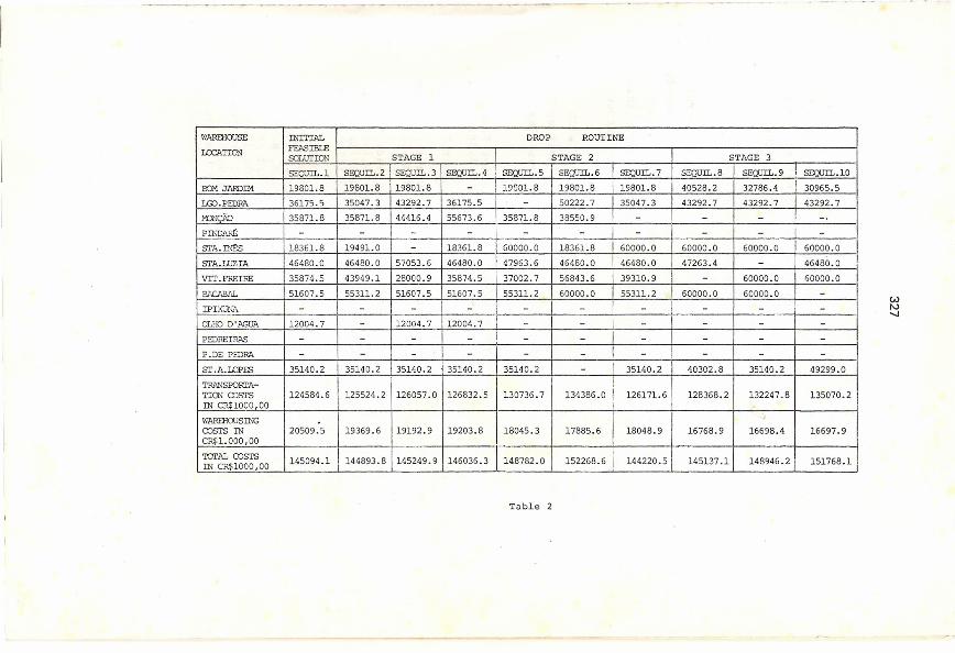
WAREHOUSE INITIAL DROP ROUTINE

ICCATICN FEASIBLESOLurION STAGE 1 STAGE 2 STAGE 3

SEÇUIL.l SEXlUIL.2 SEÇUI!..3 SEQUIL.4 SEQUIL.5 SECQIL.6 SEQUIL.7 SEQUIL.8 SEQUIL.9 SEQUIL.I0

ID'I JARDIM 19801. 8 19801. 8 19801.8 - 19301.8 19801. 8 19801.8 40528.2 32786.4 30965.5

rzo. PEDRA 36175.5 35047.3 43292.7 36175.5 - 50222.7 35047.3 43292.7 43292.7 43292.7M:NCÃO 35871. 8 35871.8 44416.4 55673.6 35871. 8 38550.9 - - - -.PTh'D1L~ - - - - - - - - - -srA.~ le3E1.8 19491.0 - 18361.8 60000.0 18361.8 60000.0 60000.0 60000.0 60000.0

si»: LUZIA 46480. O 46480. O 57053.6 46480. O 47963.6 46480. O 46480.0 47263.4 - 46480. O

VIT.FREIRE 35874.5 43949.1 28000.9 35874.5 37002.7 56843.6 39310.9 - 60000. O 60000.0

Bi\CA8AL 51607.5 55311. 2 51607.5 51607.5 55311. 2 60000.0 55311. 2 60000.0 60000.0 -IPIX"u1lA - - - - - - - - - -OLHOD'M;UA 12004.7 - 12004.7 12004.7 - - - - - -PEDREIRAS - - - - I - - - - - -P.DE PEDRA - - - - - - - - - -sr.A.WPES 35140.2 35140.2 35140.2 35140.2 35140.2 - 35140.2 40302.8 35140.2 49299.0

TRANSPORI'A-TICN CXJSrS 124584.6 125524.2 126057.0 126832.5 130736.7 134386.0 126171. 6 128368.2 132247.8 135070.2IN CR$1000, 00

NAREHOUSINGCXJSrS IN 20509.5 19369.6 19192.9 19203.8 18045.3 17885.6 18048.9 16768.9 16698.4 16697.9CR$1. 000,00

TOTALoosrs 145094.1 144893.8 145249.9 146035.3 148782.0 152268.6 144220.5 145137.1 148946.2 151768.1IN CR$1000 ,00

CAlN<r

Tab1e 2

328

al gori thm corresponds to SEQUIL 7.The whole heuristic procedure was tested for a

piecewise linear warehousing cost function (see figure 1).The obtained solution was compared with the optimal solu-tion calculated with the "Large Systems TEMPO" packageusing a Burroughs B-6700.

Total cost of optimal solution obtained by TEMPOis Cr$ 133.117.000,00 against Cr$ 133.122.352,00 for theheuristic algorithm. This corresponds to a relative errarof 0,004%. This error is negligible when we compare comput~tional times: 1848,118 seconds for TEMPO against 150,446seconds for the heuristic algorithm. We d í d not prove th a tthe heuristics are admissible and consistent in the sensedefined by HART, NILSSON and RAPHAEL 161. Thus, ouralgorithm is an approximate algorithm. Comparison w1thsolution obtained by TEMPO show however that almost optimalsolutions can be achieved within considerably less time.

1 1 I -

121 -I 3 1 -

I" I -i 5 I -

I 6 I -

I 71 -

I 8 1 -

19 I -

V. REFERENCESCANDLER,W.,J.C.SNYDER and W.FAUGHT-"Concave Programming Applied to Rice Mi11 Location"-Amer.J.Agr.Econ,1972 .ELSON,D.G.-"Site Location Via Mixed-Integer Programming"-Op.Res.Quarterly 23,31-43,1972.FELDMAN,E.,F.A.LEHER and T.L.RAY-"Warehouse Locationunder Continuous Economies of Scale"-Mngmt.Sci.12,670-687,1966.FRANK,M. and P.WOLFE-"An Algorithm for QuadraticProgramming",Naval Res.Log.Quart.3,95-110,1956.GEOFFRI ON,A. M. and G.W. GRAVES-"Mul ti commodi ty Di s tribution System Design by Benders Decomposition"-Mngmt.Sci .20,822-844, 1974.HART,P.E.,N.J.NILSSON and B.RAPHAEL-"A Formal Basisfor the Heuristic Determination of Minimum Cost Paths'IEEE Trans.of Syst.Sci.and Cyb., vol.SSC-4,nQ2, 1968.KING,G.A. and S.H.LOGAN-"Optimum Location, Number andSize of Processing Plants with Row Product and FinalProduct Shipments", J.Farm.Econ.46, 94-108,1964.KUEHN,A.A. and M.J.HAMBURGER-"A Heuristic program forLocatiilg Warehouses",Mngmt.Sci.9, 643-666,1963.SWEENEY,D.J. and R.L.TATHAN-"An Improved Long-RunModel for Multiple Warehouse Location",Mngmt.Sci.22,748-758, 1976.