


Teacher Handbook - Radiation Oncology - University of Toronto
Upload
khangminh22Category
view
1download
0

A Guide to Outcome Modeling In Radiotherapy and Oncology
Listening to the Data

Series in Medical Physics and Biomedical EngineeringSeries Editors: John G. Webster, E. Russell Ritenour, Slavik Tabakov,
and Kwan-Hoong Ng
Recent books in the series:
A Guide to Outcome Modeling In Radiotherapy and Oncology: Listening to the DataIssam El Naqa (Ed)
Advanced MR Neuroimaging: From Theory to Clinical PracticeIoannis Tsougos
Quantitative MRI of the Brain: Principles of Physical Measurement, Second editionMara Cercignani, Nicholas G. Dowell, and Paul S. Tofts (Eds)
A Brief Survey of Quantitative EEGKaushik Majumdar
Handbook of X-ray Imaging: Physics and TechnologyPaolo Russo (Ed)
Graphics Processing Unit-Based High Performance Computing in Radiation TherapyXun Jia and Steve B. Jiang (Eds)
Targeted Muscle Reinnervation: A Neural Interface for Artificial LimbsTodd A. Kuiken, Aimee E. Schultz Feuser, and Ann K. Barlow (Eds)
Emerging Technologies in BrachytherapyWilliam Y. Song, Kari Tanderup, and Bradley Pieters (Eds)
Environmental Radioactivity and Emergency PreparednessMats Isaksson and Christopher L. Rääf
The Practice of Internal Dosimetry in Nuclear MedicineMichael G. Stabin
Radiation Protection in Medical Imaging and Radiation OncologyRichard J. Vetter and Magdalena S. Stoeva (Eds)
Statistical Computing in Nuclear ImagingArkadiusz Sitek
The Physiological Measurement HandbookJohn G. Webster (Ed)
Radiosensitizers and Radiochemotherapy in the Treatment of CancerShirley Lehnert
Diagnostic EndoscopyHaishan Zeng (Ed)

Series in Medical Physics and Biomedical Engineering
Issam El NaqaAssociate Professor, University of Michigan
Ann Arbor, Michigan
A Guide to Outcome Modeling In Radiotherapy and Oncology
Listening to the Data
Boca Raton London New York
CRC Press is an imprint of theTaylor & Francis Group, an informa business
CRC PressTaylor & Francis GroupBoca Raton London New York
CRC

CRC PressTaylor & Francis Group6000 Broken Sound Parkway NW, Suite 300Boca Raton, FL 33487-2742
© 2018 by Taylor & Francis Group, LLCCRC Press is an imprint of Taylor & Francis Group, an Informa business
No claim to original U.S. Government works
Printed on acid-free paperVersion Date: 20171211
International Standard Book Number-13: 978-1-4987-6805-4 (Hardback)
This book contains information obtained from authentic and highly regarded sources. Reasonable efforts have been made to publish reliable data and information, but the author and publisher cannot assume responsibility for the validity of all materials or the consequences of their use. The authors and publishers have attempted to trace the copy-right holders of all material reproduced in this publication and apologize to copyright holders if permission to publish in this form has not been obtained. If any copyright material has not been acknowledged please write and let us know so we may rectify in any future reprint.
Except as permitted under U.S. Copyright Law, no part of this book may be reprinted, reproduced, transmitted, or utilized in any form by any electronic, mechanical, or other means, now known or hereafter invented, including photocopying, microfilming, and recording, or in any information storage or retrieval system, without written permission from the publishers.
For permission to photocopy or use material electronically from this work, please access www.copyright.com (http://www.copyright.com/) or contact the Copyright Clearance Center, Inc. (CCC), 222 Rosewood Drive, Danvers, MA 01923, 978-750-8400. CCC is a not-for-profit organization that provides license and registration for a variety of users. For organizations that have been granted a photocopy license by the CCC, a separate system of payment has been arranged.
Trademark Notice: Product or corporate names may be trademarks or registered trademarks, and are used only for identification and explanation without intent to infringe.
Visit the Taylor & Francis Web site athttp://www.taylorandfrancis.com
and the CRC Press Web site athttp://www.crcpress.com
Library of Congress Cataloging-in-Publication Data
Names: El Naqa, Issam, editor.Title: A guide to outcome modeling in radiotherapy and oncology : listening to the data / edited by Issam El Naqa.Other titles: Series in medical physics and biomedical engineering.Description: Boca Raton, FL : CRC Press, Taylor & Francis Group, [2018] | Series: Series in medical physics and biomedical engineering | Includes bibliographical references and index.Identifiers: LCCN 2017036390 | ISBN 9781498768054 (hardback ; alk. paper) | ISBN 1498768059 (hardback ; alk. paper) | ISBN 9781498768061 (e-book) | ISBN 1498768067 (e-book)Subjects: LCSH: Cancer--Radiotherapy--Data processing. | Oncology--Dataprocessing. Classification: LCC RC271.R3 G85 2018 | DDC 616.99/40642--dc23LC record available at https://lccn.loc.gov/2017036390

To my parents (Rola & Mustafa), brothers (Rami & Rabie),my wife Rana and daughters (Layla & Lamees).

Contents
Section I Multiple Sources of Data
Chapter 1 � Introduction to data sources and outcome models 3Issam El Naqa and Randall K. Ten Haken
1.1 INTRODUCTION TO OUTCOME MODELING 41.2 MODEL DEFINITION 41.3 TYPES OF OUTCOME MODELS 6
1.3.1 Prognostic versus predictive models 6
1.3.2 Top-down versus bottom-up models 6
1.3.3 Analytical versus data-driven models 7
1.4 TYPES OF DATA USED IN OUTCOME MODELS 91.5 THE FIVE STEPS TOWARDS BUILDING AN OUTCOME MODEL 91.6 CONCLUSIONS 11
Chapter 2 � Clinical data in outcome models 13Nicholas J. DeNunzio, MD, PhD, Sarah L. Kerns, PhD, and Michael T Milano, MD, PhD
2.1 INTRODUCTION 142.2 COLLAGEN VASCULAR DISEASE 162.3 GENETIC STUDIES 172.4 BIOLOGICAL FACTORS IMPACTING TOXICITY AFTER SBRT 19
2.4.1 Chest wall toxicity after SBRT 20
2.4.2 Radiation-induced lung toxicity (RILT) after SBRT 20
2.4.3 Radiation-induced liver damage (RILD) after SBRT 22
2.5 BIG DATA 232.6 CONCLUSIONS 23
Chapter 3 � Imaging data (radiomics) 25Issam El Naqa
3.1 INTRODUCTION 253.2 IMAGE FEATURES EXTRACTION 26
3.2.1 Static image features 26
3.2.2 Dynamic image features 27
3.3 RADIOMICS EXAMPLES FROM DIFFERENT CANCER SITES 283.3.1 Predicting local control in lung cancer using PET/CT 28
vii

viii � Contents
3.3.2 Predicting distant metastasis in sarcoma using PET/MR 30
3.4 CONCLUSIONS 31
Chapter 4 � Dosimetric data 33Issam El Naqa and Randall K. Ten Haken
4.1 INTRODUCTION 344.2 DOSE VOLUME METRICS 354.3 EQUIVALENT UNIFORM DOSE 364.4 DOSIMETRIC MODEL VARIABLE SELECTION 38
4.4.1 Model order based on information theory 38
4.4.2 Model order based on resampling methods 38
4.5 A DOSIMETRIC MODELING EXAMPLE 394.5.1 Data set 39
4.5.2 Data exploration 40
4.5.3 Multivariate modeling with logistic regression 41
4.5.4 Multivariate modeling with machine learning 42
4.5.5 Comparison with other known models 43
4.6 SOFTWARE TOOLS FOR DOSIMETRIC OUTCOME MODELING 444.7 CONCLUSIONS 45
Chapter 5 � Pre-clinical radiobiological insights to inform modelling ofradiotherapy outcome 47Peter van Luijk, PhD and Robert P. Coppes, PhD
5.1 VARIABILITY IN RESPONSE TO HIGHLY STANDARDIZED RADIO-THERAPY 48
5.2 VARIATION IN SENSITIVITY TO RADIATION 495.3 UNDERSTANDING DOSE-RESPONSE OF TISSUES AND ORGANS 505.4 ANIMAL MODELS TO STUDY RADIATION RESPONSE 505.5 PROCESSES GOVERNING OUTCOME 515.6 PATIENT-INDIVIDUAL FACTORS / CO-MORBIDITY 525.7 USE IN MODELS 525.8 CONCLUSION 52
Chapter 6 � Radiogenomics 53Issam El Naqa, Sarah L. Kerns, PhD, James Coates, PhD, Yi Luo, PhD, Corey Speers,MD PhD, Randall K. Ten Haken, Catharine M.L. West, PhD, and Barry S. Rosenstein, PhD
6.1 INTRODUCTION 546.2 BIOMARKERS AND THE WORLD OF “-OMICS” 54
6.2.1 Structural variations 56
6.2.1.1 Single nucleotide polymorphisms (SNPs) 56
6.2.1.2 Copy number variations (CNVs) 56
6.2.2 Gene expression: mRNA, miRNA, lncRNA 57

Contents � ix
6.2.3 Protein expression 57
6.2.4 Metabolites 59
6.3 RESOURCES FOR BIOLOGICAL DATA 596.4 EXAMPLES OF RADIOGENOMIC MODELING 60
6.4.1 Prostate cancer 60
6.4.2 Breast cancer 61
6.4.3 Lung cancer 61
6.5 CONCLUSIONS 62
Section II Top-down Modeling Approaches
Chapter 7 � Analytical and mechanistic modeling 65Vitali Moiseenko, PhD, Jimm Grimm, PhD, James D. Murphy, PhD, David J. Carlson,PhD, and Issam El Naqa, PhD
7.1 INTRODUCTION 667.2 TRACK STRUCTURE AND DNA DAMAGE 677.3 LINEAR-QUADRATIC MODEL 697.4 KINETIC REACTION RATE MODELS 73
7.4.1 Repair-misrepair and lethal-potentially-lethal models 73
7.4.2 Refined models 74
7.4.3 The Giant LOop Binary LEsion (GLOBE) 75
7.4.4 Local Effect Model (LEM) 75
7.4.5 Microdosimetric-kinetic model (MKM) 76
7.4.6 The Repair-misrepair-fixation model 76
7.5 MECHANISTIC MODELING OF STEREOTACTIC RADIOSURGERY(SRS) AND STEREOTACTIC BODY RADIOTHERAPY (SBRT) 777.5.1 LQ limitations and alternative models 79
7.6 INCORPORATING BIOLOGICAL DATA TO DESCRIBE AND PREDICTBIOLOGICAL RESPONSE 81
7.7 CONCLUSIONS 82
Chapter 8 � Data driven approaches I: conventional statistical inferencemethods, including linear and logistic regression 85Tiziana Rancati and Claudio Fiorino
8.1 WHAT IS A REGRESSION 868.2 LINEAR REGRESSION 87
8.2.1 Mathematical formalism 88
8.2.2 Estimation of regression coefficients 88
8.2.3 Accuracy of coefficient estimates 89
8.2.4 Rejecting the null hypothesis 89
8.2.5 Accuracy of the model 90
8.2.6 Qualitative predictors 91

x � Contents
8.2.7 Including interactions between variables 92
8.2.8 Linear regression: example 93
8.3 LOGISTIC REGRESSION 1018.3.1 Modelling of qualitative (binary) response 101
8.3.2 Mathematical formalism 103
8.3.3 Estimation of regression coefficients 105
8.3.4 Accuracy of coefficient estimates 105
8.3.5 Rejecting the null hypothesis, testing the significance of amodel 106
8.3.6 Accuracy of the model 106
8.3.7 Qualitative predictors 108
8.3.8 Including interaction between variables 108
8.3.9 Statistical power for reliable predictions 108
8.3.10 Time consideration 109
8.4 MODEL VALIDATION 1098.4.1 Apparent validation 111
8.4.2 Internal validation 111
8.4.3 External validation 112
8.5 EVALUATION OF AN EXTENDED MODEL 1138.6 FEATURE SELECTION 113
8.6.1 Classical approaches 114
8.6.2 Shrinking and regularization methods: LASSO 115
8.6.3 Bootstrap methods 116
8.6.4 Logistic regression: example 118
8.7 CONCLUSIONS 127
Chapter 9 � Data driven approaches II: Machine Learning 129Sarah Gulliford, PhD
9.1 INTRODUCTION 1309.2 FEATURE SELECTION 132
9.2.1 Principal Component Analysis (PCA) 132
9.2.1.1 When should you use them? 133
9.2.1.2 Who has already used them? 133
9.3 FLAVORS OF MACHINE LEARNING 1349.3.1 Artificial Neural Networks 134
9.3.1.1 The basics 134
9.3.1.2 When should you use them? 136
9.3.1.3 Who has already used them? 136
9.3.2 Support Vector Machine 137
9.3.2.1 The basics 137
9.3.2.2 When should you use them? 137

Contents � xi
9.3.2.3 Who has already used them? 138
9.3.3 Decision Trees and Random Forests 138
9.3.3.1 The basics 138
9.3.3.2 When should you use them? 139
9.3.3.3 Who has already used them? 139
9.3.4 Bayesian approaches 140
9.3.4.1 The basics 140
9.3.4.2 When should you use them? 140
9.3.4.3 Who has already used them? 141
9.4 PRACTICAL IMPLEMENTATION 1429.4.1 The data 142
9.4.2 Model fitting and assessment 142
9.5 CONCLUSIONS 1439.6 RESOURCES 143
Section III Bottom-up Modeling Approaches
Chapter 10 � Stochastic multi-scale modeling of biological effects inducedby ionizing radiation 147Werner Friedland and Pavel Kundrat
10.1 INTRODUCTION 14810.2 PARTICLE TRACKS: PHYSICAL STAGE 15110.3 PARTICLE TRACKS: PHYSICO-CHEMICAL AND CHEMICAL STAGE 16110.4 MULTI-SCALE DNA AND CHROMATIN MODELS 16510.5 INDUCTION OF DNA AND CHROMATIN DAMAGE 16910.6 DNA DAMAGE RESPONSE 17210.7 MODELING BEYOND SINGLE-CELL LEVEL 17910.8 CONCLUSIONS 180
Chapter 11 � Multi-scale modeling approaches: application in chemo– andimmuno–therapies 181Issam El Naqa
11.1 INTRODUCTION 18211.2 MEDICAL ONCOLOGY TREATMENTS 183
11.2.1 From chemotherapy to molecular targeted agents 183
11.2.2 Immunotherapy 184
11.3 MODELING TYPES 18511.3.1 Continuum tumor modeling 185
11.3.2 Discrete tumor modeling 188
11.3.3 Hybrid tumor modeling 189
11.4 MODELING EXAMPLES 19011.4.1 Modeling of chemotherapy 190

xii � Contents
11.4.2 Modeling of immunotherapy 192
11.5 SOFTWARE TOOLS FOR MULTI-SCALE MODELING 19311.6 CONCLUSIONS 194
Section IV Example Applications in Oncology
Chapter 12 � Outcome modeling in treatment planning 197X. Sharon Qi, Mariana Guerrero, and X. Allen Li
12.1 INTRODUCTION 19912.1.1 Review of the history and dose-volume based treatment plan-
ning and its limitations 199
12.1.2 Emerging dose-response modeling in treatment planning andadvantages 200
12.2 DOSE-RESPONSE MODELS 20212.2.1 Generalized equivalent uniform dose (gEUD) 202
12.2.1.1 Serial and parallel organ models 202
12.2.2 Linear-Quadratic (LQ) Model 203
12.2.3 Biological effective dose (BED) 204
12.2.4 Tumor control probability (TCP) models 204
12.2.5 Normal Tissue Complication Model (NTCP) models 206
12.2.5.1 Lyman-Kutcher-Burman (LKB) model 206
12.2.5.2 Relative seriality (RS) model 207
12.2.5.3 Model parameters and Quantitative Analysis ofNormal Tissue Effects in the Clinic (QUANTEC) 207
12.2.6 Combined TCP/NTCP models –Uncomplicated tumor con-trol model (UTCP or P+) 208
12.3 DOSE-RESPONSE MODELS FOR STEREOTACTIC BODYRADIOTHERAPY (SBRT) 20812.3.1 Linear-Quadratic (LQ) model applied to SBRT 208
12.3.2 Universal survival curve (USC) model 209
12.3.3 Linear-Quadratic-Linear (LQL) model 210
12.3.4 Regrowth model 211
12.3.5 Dose limits for SBRT treatments 211
12.4 BIOLOGICAL MODELS IN TREATMENT PLANNING 21412.4.1 Plan evaluation 214
12.4.2 Plan optimization 215
12.4.3 Dose summation using biological models 215
12.4.4 Selection of outcome models and model parameters 216
12.5 COMMERCIALLY AVAILABLE TREATMENT PLANNING SYSTEMS (TPS)EMPLOYING OUTCOME MODELS 21612.5.1 Elekta Monaco system (Maryland Heights, MO) 216
12.5.2 Philips Pinnacle system (Andover, MA) 218
12.5.2.1 Sensitivity of model parameters 219

Contents � xiii
12.5.3 Varian Eclipse system (Palo Alto, CA) 220
12.5.3.1 Objective functions in plan optimization 220
12.5.3.2 Plan evaluation 221
12.5.3.3 Sensitivity of model parameters 222
12.5.4 RaySearch RayStation (Stockholm, Sweden) 222
12.5.4.1 Plan evaluation tools 222
12.5.4.2 Plan optimization tools 222
12.5.5 MIM (MIM Software Inc., Cleveland, OH) 222
12.5.5.1 Plan summation 223
12.5.5.2 Plan evaluation 223
12.6 CONCLUSIONS 224
Chapter 13 � A utility based approach to individualized and adaptiveradiation therapy 225Matthew J Schipper, PhD
13.1 INTRODUCTION 22613.2 BACKGROUND 226
13.2.1 Treatment planning in radiation therapy 226
13.2.2 Biomarkers in RT 227
13.3 UTILITY APPROACH TO PLAN OPTIMIZATION 22913.3.1 In phase I trials 229
13.3.2 In RT treatment planning 229
13.3.3 Choice of the tradeoff parameter 231
13.3.4 Virtual clinical trial 231
13.4 CONCLUSIONS 234
Chapter 14 � Outcome modeling in Particle therapy 235J. Schuemann, A.L. McNamara, and C. Grassberger
14.1 HOW ARE PARTICLES DIFFERENT FROM PHOTONS? 23614.2 LINEAR ENERGY TRANSFER (LET) 238
14.2.1 Dose averaging, track averaging and limitations 238
14.3 RELATIVE BIOLOGICAL EFFECTIVENESS 24014.3.1 The 1.1 conundrum in proton therapy 241
14.3.2 LET based RBE models 242
14.3.3 Non-LET based 244
14.3.3.1 Track structure (δ-ray) model 246
14.3.4 Uncertainties 247
14.4 THE ROLE OF MONTE CARLO 24814.4.1 Understanding dose and LET distributions 248
14.4.1.1 Range uncertainties 248
14.4.1.2 Considerations for dose and DVH 250

xiv � Contents
14.4.1.3 LET 250
14.4.2 RBE modeling 252
14.4.3 Example MC simulations using TOPAS 252
14.4.3.1 2-spot pencil setup 252
14.4.3.2 Expansion to include patient setup, dose, LET andone RBE scorer 253
14.5 IMPLICATIONS OF PARTICLE THERAPY FOR OUTCOME MODELS 25314.5.1 Target effects 254
14.5.2 Normal Tissue effects 255
14.6 APPLICATION IN TREATMENT PLANNING 25514.6.1 Vision for the future 256
Chapter 15 � Modeling response to oncological surgery 259J. Jesus Naveja, Leonardo Zapata-Fonseca, and Flavio F. Contreras-Torres
15.1 INTRODUCTION TO ONCOLOGICAL SURGERY 26015.1.1 Clinical and surgical factors modifying patients’ outcomes 260
15.1.2 Complementary therapies to oncological surgery 261
15.2 MODELING OF ONCOLOGICAL SURGERY 26215.2.1 Computational oncology models 262
15.2.2 Mechanistic models from physical oncology 264
15.2.2.1 Relevant variables 264
15.2.2.2 Implemented models 266
15.3 EXAMPLE: A BIDIMENSIONAL ONCOLOGICAL SURGERYSIMULATION MODEL 26715.3.1 Step 1: diffusion of nutrients 268
15.3.2 Step 2: CA rules and tumor growth constrained by the nu-trients concentration and immune system response 269
15.3.3 Step 3: surgery 271
15.4 DISCUSSION 27415.5 CONCLUSIONS AND PERSPECTIVES 27415.6 APPENDIX 1: R CODE 275
Chapter 16 � Tools for the precision medicine era: developing highlyadaptive and personalized treatment recommendations us-ing SMARTs 283Elizabeth F. Krakow and Erica E. M. Moodie
16.1 INTRODUCTION 28416.2 STUDYING TREATMENTS IN SEQUENCE 285
16.2.1 Adaptive treatment strategies 285
16.2.2 Decision rules 285
16.2.3 Tailoring variables are key for personalized recommendations 285
16.2.4 Machine learning “teaches” us the optimal ATS 288

Contents � xv
16.3 COMPARISON TO TRADITIONAL METHODS 29016.3.1 Why might RCTs fail to identify good treatment sequences? 290
16.3.2 Why can’t we combine results from separate, single-stageRCTs? 291
16.3.3 What are the advantages of SMARTs? 293
16.3.4 Motivating example 294
16.4 VALIDATING A PROPOSED ATS 29416.4.1 If we find an optimal ATS with a SMART, do we still need
an RCT? 294
16.4.2 Are SMARTs used in cancer? 296
16.5 CHALLENGES AND OPPORTUNITIES 297
Index 365

Foreword First edition
The goal of medicine is to improve the lives of our patients as much as possible while notcausing harm. In my over 30 years as an attending radiation oncologist, I have tried todo this through reading, attending lectures, and thinking deeply about my successes andfailures among the thousands of patients I have treated during my career. But how toorganize all of this information in a way that is most beneficial to our patients? There iswell-worn joke in medicine about the “physician” (pick your favorite specialty to tease) whohas seen one patient, two patients, or three patients with a particular problem, and whospouts, with great authority, “In my experience”, “In my series”, or “In case after case aftercase”. Likewise, the standard saying in medicine, “Three anecdotes? That’s data!” Surely,in this era of “Big Data” we can do better for our patients than thinking of the last timewe saw a patient who was similar to the one in front of us, and hoping to treat this newpatient the same way, if our prior treatment was successful, or differently, if treatment wasunsuccessful.
The answer is yes! This informative multi-author book edited by Dr. Issam El Naqagives us insights into how we can organize our data by using models that can predict,and, thereby improve the outcome of treatment. Chapters are devoted to the input, suchas incorporating clinical, imaging, dosimetric data, as well as modern radiation biology,and how to use those data to build models that will improve the physician’s ability tobalance efficacy and toxicity far more accurately than relying on pure clinical judgement.This book is coming at a particularly good time. The tsunami of data to which we nowhave access overwhelms the physician’s ability for incorporation into a treatment plan, butis too valuable to ignore. At the University of Michigan, we are using these models to helpus make treatment decisions. Even when we do not yet feel that the data are strong enoughto build a robust model for predicting outcome, these models help to organize our approachand aim us toward the data we need to gather to improve our clinical decision making.
An unusual feature of this book is brilliance of the editor. Multi-author books are oftenuneven, with gaps and repetitions resulting from the lack of unifying force. Dr. El Naqa’sremarkable breadth of knowledge gives this book a unity rarely found in such texts andgreatly increases its value.
Big Data are here to stay. . . and will only get Bigger. This book can help us turn datainto knowledge, and, perhaps, wisdom.
Theodore S. Lawrence, MD, PhD, FASTRO, FASCOIsadore Lampe Professor and ChairDepartment of Radiation Oncology
University of Michigan
xvii

Foreword First edition
Over the past 50 years, several books have been written on the subject of outcome modelingin radiation oncology. They illustrate a continuous progress in our understanding of effectsof radiation treatment on cancer and normal tissues, and progress in methodology of analyz-ing ever increasing pool of clinical and experimental data. This book, edited by Dr. El Naqa,clearly indicates that the field of outcome modeling is changing rapidly and in a qualitativeway. That is, several book chapters cover subject matters that did not even exist not longago. For example, book chapters on machine learning, radiomics, or radiogenomics, presentnew and exciting areas of active research that may lead to improved outcomes of cancertreatment. Chapter 1 is an excellent introduction to the subject of outcome modeling, andthe last Chapter 16 discusses the challenges and opportunities in the era of personalizedmedicine. The remaining 14 chapters are divided into four logical sections on sources of data,top-down modeling approaches, bottom-up modeling approaches, and example applicationsin oncology. All chapters are well-written and present in-depth discussion of state-of-the-artin the respective areas. The book is very well edited and should be on a must-read list foranyone who is interested in outcome modeling research. For someone who has been doingoutcome modeling for over 30 years, the book also well illustrates one of my favourite quotesattributed to Albert Einstein “The more I learn, the more I realize how much I don’t know.”It rings very true for me personally, and this book will be a valuable addition to my library.However, it also applies to the entire field of outcome modeling. Finding or developing the“final” and “true” model of relevant outcomes in oncology is still as challenging, and asexciting, as ever before. All 300 hundred or so pages of this book well illustrate both, thechallenges and the excitement of new approaches and possible solutions that may improvethe outcomes of treatment for patients with cancer.
Andrzej Niemierko, Ph.D.Associate Professor of Radiation OncologyInstitution Massachusetts General Hospital
Radiation Oncology DepartmentHarvard University, Massachusetts General Hospital 10
Emerson #122, Boston MA 02114email: [email protected] Phone 617/724-9527
xix

Preface
OUTCOME modeling in radiation oncology and the broader oncology field plays animportant part in understanding response, designing clinical trials, and personaliz-
ing patients’ treatment. It attempts to provide an approximate representation of a verycomplex cancer environment within an individual patient or population of patients. Thisrepresentation would allow for predicting response to known therapeutic interventions andfurther extrapolate this treatment effect beyond current standards. Modeling of outcomeshas accompanied cancer treatments since its early days. Initially, this was based on cognitiveunderstanding of the disease, accumulated experiences and simplistic understanding of ob-served effects clinically or experimentally. This was based primarily on using in vitro assays,which constituted the basis for developing analytical or sometimes refereed to asmechanisticmodels of response, which have been applied widely for predicting response and designingearly clinical trials over the past century. However, due to the inherent complexity andheterogeneity of biological processes, these traditional modeling methods have fallen shortof providing sufficient predictive power when applied prospectively to personalize treatmentregimens. Therefore, more modern approaches are investigating more data-driven, advancedinformatics, and systems engineering techniques that are able to integrate physical and bio-logical information and to adapt intra-treatment changes and optimize post-treatment out-comes using top-down approaches based on big data complex system analyses or bottom-uptechniques based on first principles and multi-scale approaches.
The original idea of this book was conceived by the editor’s own (re)search for a compre-hensive resource on outcome modeling and was encouraged by discussions with colleaguesand trainees whom where looking into materials that could help them get their initial footinginto this mystifying field of developing outcomes models; as part of their practice to under-stand already existing ones or to learn the field to become a new contributor with new freshand unexplored ideas. The world of outcome modeling is too vast to be covered in singlevolume and every one working in the field of oncology whether directly or indirectly is alikely contributor. Who is in the field of oncology is not curious or is not tempted to predictwhat will happen with a treated patient? However, in this book we confine ourselves to thecomputational aspects that would use existing information (knowledge and/or data) as aresource and feed this resource into a suitable mathematical framework that could relate thestream of current information to a futuristic clinical endpoint such as local control, toxicity,or survival. A book of this nature can not be written by a single individual with specializedexpertise, but it draws on the knowledge and wisdom of many experts from many domainsincluding but not limited to clinical practitioners, biologists, physicists, computer scientists,statisticians, bioinformaticians, all are more than happy to call themselves M odelers whocontinue to learn from each other. Personally, I’ve been fortunate to gain my first stepsinto outcome modeling from Dr. Joseph O. Deasy and continue to explore its deep horizonswith Dr. Randall T. Ten Haken, to whom I’m very grateful for their mentorship, guidance,and friendship. I would like also to acknowledge our clinical colleagues, particularly Dr.Jeffrey D. Bradley and the team at Washington University in St. Louis including Dr. An-drew Hope and Dr. Patricia Lindsay; and the team at McGill University led by Dr. Jan
xxi

xxii � Preface
Seuntjens and Dr. Carolyn Freeman; and the many colleagues and collaborators that I hadthe privilege to work with on many of the studies cited in this book. I would like also toacknowledge my trainees’ invaluable contributions from them I learned possibly as much asI taught them. Ultimately, the goal of such a textbook is to provide a didactic path to out-come modeling in oncology as a promising tool as well as fulfilling a duty to serve our cancerpatients and improve their care and quality of life through advanced education and research.
The book is an open invitation to the world of outcome modeling in oncology and itsesteemed modelers, where basic science meets data science, art is embedded in Greek let-ters and Arabic numerals, skill is highlighted in computer coding, intuition is expressed inmathematical formulas, and prediction aims to give cancer patients and their caregiversnew light and genuine hope in their treatment choices.
In a data-centric world, the first section of the book aims to provide the reader withoverview information about the different and heterogeneous data sources and resourcesthat could be all or partly used in model design and building. These data could be clinicalor preclinical, and could span basic patient and/or treatment characteristics, to medicalimaging and their features (radiomics) into more molecular biological markers (genomics,proteomics, metabolomics, etc.) constituting the so called pan-omics of oncology, generatedover a treatment period that can span a few days to several weeks or months.
The second and the third sections of the book, aim to introduce the two main categoriesof outcome modeling according to their design methodology, namely; top-down and bottomapproaches. The top-down approaches are presented in section II, starting with analytical(mechanistic models) through conventional statistical approaches into advanced machinelearning techniques, which are currently the cornerstone of the Big Data era. Section IIIpresents bottom-up approaches using first principles and multi-scale techniques with numeri-cal simulations based on Monte Carlo with application in radiotherapy and non-Monte Carloapproaches with application in chemotherapy and immunotherapy. Description of softwaresand tools for development and evaluation was intentionally embedded into most of thesechapters to make it more accessible to learn hands-on by example and also experiment withmany of the featured modeling approaches.
The fourth and last section of the books presents a diverse selection of common ap-plications of outcome modeling from a wide variety of areas: treatment planning in radio-therapy, utility-based and biomarker applications, particle therapy modeling, oncologicalsurgery, and design of adaptive and SMART clinical trials. These applications aim to serveas demonstrations of the potential power of outcome modeling in personalizing medicinein oncology, as well as samples to highlight technical issues and challenges that may ariseduring the processes of model building and evaluation when applied to real-life clinicalproblems.

Contributors
David J. Carlson, PhDDepartment of Radiation Oncology,Yale University, New Haven, CT, USA
James Coates, PhDDepartment of Oncology,University of Oxford, Oxford, UK
Flavio F. Contreras-Torres, PhDCentro del Agua para America Latina y el
Caribe.Tecnologico de Monterrey, Monterrey,
Mexico
Robert P. Coppes, PhDDepartments of Radiation Oncology and
Cell Biology,University Medical Center Groningen,
Groningen, the Netherlands
Nicholas J. DeNunzio, MD, PhDDepartment of Radiation Oncology,University of Rochester, 601 Elmwood Ave.
Box 647, Rochester, NY, USA
Issam El Naqa, PhDDepartment of Radiation Oncology,University of Michigan, Ann Arbor, MI,
USA
Claudio Fiorino, PhDMedical Physics Department,San Raffaele Scientific Institute, Milan,
Italy
Werner Friedland, PhDHelmholtz Zentrum Munchen - German
Research Center for EnvironmentalHealth (GmbH),
Institute of Radiation Protection,Neuherberg, Germany
C. Grassberger, PhDDepartement of Radiation Oncology,Massachusetts General Hospital & Harvard
Medical School, Boston, MA, USA
Jimm Grimm, PhDDepartment of Radiation Oncology,Johns Hopkins University, Baltimore, MD,
USA
Mariana Guerrero, PhDDepartment of Radiation Oncology,University of Maryland School of Medicine,
Baltimore, MD 21201, USA
Sarah Gulliford, PhDThe Institute of Cancer Research,Sutton, Surrey SM2 5NG, UK
Sarah L. Kerns, PhDDepartment of Radiation Oncology,University of Rochester, Rochester, NY,
USA
Elizabeth F. Krakow, PhDDivision of Clinical Research, Fred
Hutchinson Cancer Research Center andDepartment of Medical Oncology,
University of Washington, Washington,USA
Pavel Kundrat, PhDHelmholtz Zentrum Munchen - German
Research Center for EnvironmentalHealth (GmbH),
Institute of Radiation Protection,Neuherberg, Germany
X. Allen Li, PhDDepartment of Radiation Oncology,Medical College of Wisconsin, Milwaukee,
WI 53226, USA
xxiii

xxiv � Contributors
Yi Luo, PhDDepartment of Radiation Oncology,University of Michigan, Ann Arbor, MI,
USA
A.L. McNamara, PhDDepartment of Radiation Oncology,Massachusetts General Hospital & Harvard
Medical School, Boston, MA, USA
Michael T Milano, MD, PhDDepartment of Radiation Oncology,University of Rochester, 601 Elmwood Ave.
Box 647, Rochester, NY, USA
Vitali Moiseenko, PhDDepartment of Radiation Medicine and
Applied Sciences,University of California San Diego, La
Jolla, CA, USA
Erica E. M. Moodie, PhDDepartment of Epidemiology, Biostatistics
& Occupational Health,McGill University, Quebec, Canada
James D. Murphy, PhDDepartment of Radiation Medicine and
Applied Sciences,University of California San Diego, La
Jolla, CA, USA
J. Jesus Naveja, PhDPECEM. Facultad de Medicina,Universidad Nacional Autonoma de Mexico,
Mexico City, Mexico
X. Sharon Qi, PhDDepartment of Radiation Oncology,UCLA school of Medicine, Los Angeles, CA
90095, USA
Tiziana Rancati, PhDProstate Cancer Program,Fondazione IRCCS Istituto Nazionale dei
Tumori, Milan, Italy
Barry S. Rosenstein, PhDDepartments of Radiation Oncology and
Genetics and Genomic Sciences,Icahn School of Medicine at Mount Sinai,
New York, NY, USA
Matthew J Schipper, PhDDepartments of Radiation Oncology and
Biostatistics,University of Michigan, MI, USA
J. Schuemann, PhDDepartement of Radiation Oncology,Massachusetts General Hospital & Harvard
Medical School, Boston, MA, USA
Corey Speers, MD PhDDepartment of Radiation Oncology,University of Michigan, Ann Arbor, MI,
USA
Randall K. Ten Haken, PhDDepartment of Radiation Oncology,University of Michigan, Ann Arbor, MI,
USA
Catharine M.L. West, PhDDivision of Cancer Sciences, Manchester
Academic Health Science Centre,Christie Hospital NHS Trust,
University of Manchester, Manchester, UK
Peter van Luijk, PhDDepartment of Radiation Oncology,University Medical Center Groningen,
Groningen, the Netherlands
Leonardo Zapata-Fonseca, PhDPECEM. Facultad de Medicina,Universidad Nacional Autonoma de Mexico,
04600, Mexico City, Mexico

IMultiple Sources of Data
1

C H A P T E R 1
Introduction to data sourcesand outcome modelsIssam El Naqa
Randall K. Ten Haken
CONTENTS
1.1 Introduction to outcome modeling . . . . . . . . . . . . . . . . . . . . . . . . . . . . . . . . . . . . . 41.2 Model definition . . . . . . . . . . . . . . . . . . . . . . . . . . . . . . . . . . . . . . . . . . . . . . . . . . . . . . . . 41.3 Types of outcome models . . . . . . . . . . . . . . . . . . . . . . . . . . . . . . . . . . . . . . . . . . . . . . . 6
1.3.1 Prognostic versus predictive models . . . . . . . . . . . . . . . . . . . . . . . . . . . . 61.3.2 Top-down versus bottom-up models . . . . . . . . . . . . . . . . . . . . . . . . . . . . 61.3.3 Analytical versus data-driven models . . . . . . . . . . . . . . . . . . . . . . . . . . . 7
1.4 Types of data used in outcome models . . . . . . . . . . . . . . . . . . . . . . . . . . . . . . . . . 91.5 The five steps towards building an outcome model . . . . . . . . . . . . . . . . . . . . 91.6 Conclusions . . . . . . . . . . . . . . . . . . . . . . . . . . . . . . . . . . . . . . . . . . . . . . . . . . . . . . . . . . . . . 11
ABSTRACTOutcome modeling plays a pivotal role in oncology. This includes understanding responseto different therapeutic cancer agents, personalization of treatment and designing of futureclinical trials. Although application of outcome models has accompanied oncology prac-tices since its inception, it also evolved from simple hand calculations of doses based onexperiences and simplified understanding of cancer behavior into more advanced computersimulation models driven by tremendous growth in patient-specific data and an acute de-sire to have more accurate predictions of response. This chapter reviews basic definitionsused in computational modeling and main data resources, and provides an overview of theincreasing role of outcome models in the field of oncology.
Keywords: outcome models, oncology, data, applications.
3

4 � A Guide to Outcome Modeling in Radiotherapy and Oncology
1.1 INTRODUCTION TO OUTCOME MODELING
Modeling is a process of generating an abstract representation of a subject. In the con-text of outcomes, this process entails identifying the underlying relationship between
observed clinical outcomes and the different types of data that generated them. Modelsin their inherent nature are approximations of relationships between the observations andthe data, otherwise, they would be considered as laws of nature such as Newton’s laws ofmotion, for instance. This notion was perhaps best articulated by George Box, a renownedstatistician, who famously stated: “All models are wrong but some are useful” [1]. Thisstatement should be kept as a reminder that models are often idealized simplifications ofreality and may not be the “truth” sought after [2]. However, their usefulness should bejudged depending on their ability to solve the problem at hand. In case of outcome models,this would be translated into the ability of such models to sufficiently predict a patient’sresponse to a certain treatment regimen given known relevant characteristics of the pa-tient, the disease, and the treatment itself. The question of sufficiency is tied to the desiredpredictive power of the model and its ability to differentiate between high and low riskpatient outcomes. On the other hand, the relevancy of the model characteristics is relatedto the data types employed and the minimum number of variables needed in a model tomake it predictive. This is succinctly summarized in another famous quote from AlbertEinstein: “Everything should be made as simple as possible, but no simpler.” This is animportant principle in modeling known as parsimony or the Occam’s razor, which advocatesthat among all the models representing available observations, the simplest one is the mostplausible one [3]. However, this should be cautiously applied and is actually contradictedin the case of mechanistic or systems biology approaches, where it is implied that by incor-porating more assumptions into a model (not necessarily for the purpose of improving thepredictive power) will allow the learning and extracting of more information from the dataat the possible expense of risking more uncertainty [4].
The process of outcome modeling, following early attempts to systematically apply ther-apeutic agents at the end of the 19th century, has continuously evolved from trial and errorapproaches with back of the envelope hand calculations into the application of advancedstatistical and mathematical techniques. Modeling has long been recognized as a usefultool to synthesize existing knowledge, test new treatment scenarios that may not have beenobserved in clinical trials, and compare different treatment regimens. This role has been fur-ther invigorated by advances in patient-specific information, biotechnology, imaging, andcomputational capabilities. In the era of big data and personalized or precision medicine,it is expected that outcome modeling will be at the center of these initiatives paving theway to better understanding of cancer biology and its response to treatment. It is currentlyspearheading the process of development of appropriate clinical decision support systemsfor cancer management across the spectrum of available treatment modalities to achieve animproved quality of care for cancer patients [5].
1.2 MODEL DEFINITIONThe Merriam-Webster Dictionary defines a model “as a system of postulates, data, andinferences presented as a mathematical description of an entity or state of affairs” while theOxford Dictionary defines it as “a simplified description, especially a mathematical one, ofa system or process, to assist calculations and predictions.” In the context of computationalmodeling, the National Institute of Biomedical Imaging and Bioengineering (NIBIB) definesit as the use of mathematics, physics and computer science to study the behavior of complex

Introduction to data sources and outcome models � 5
systems by computer simulation to make predictions about what will happen in the realsystem that is being studied in response to changing conditions. For the purpose of outcomemodeling in oncology, we modify this definition as follows:
Definition 1.1 Outcome modeling is the general process of using mathematics, statistics,physics, biology, and computer science to characterize the behavior of tissue response to atreatment (radiation, drug, surgery, etc.) such as tumor eradication (control) or side effects(toxicities) via approximate computer simulations in order to make predictions about whatwill happen in the patient under changing therapy conditions.
Outcome models can help to understand the underlying biology of cancer response totreatment. They can approximate the treatment environment and be used to develop de-cision support tools for oncologists that can provide guidance for treatment or design offuture clinical trials as depicted in Figure 1.1.
Figure 1.1 The process of outcome modeling as an approximation of the real world
by mathematical constructs that would allow future prediction of response and
comparison with future treatment responses.

6 � A Guide to Outcome Modeling in Radiotherapy and Oncology
1.3 TYPES OF OUTCOME MODELSOutcome models can be generally categorized: (1) based on their objective into predictiveor prognostic; (2) based on their methodology into top-down or bottom-up approaches; and(3) based on their assumptions into analytical and data-driven models.
1.3.1 Prognostic versus predictive modelsA model could be categorized into being a predictive or prognostic model depending onwhether the treatment parameters are considered as part of the model construction or not,respectively. A prognostic model can inform about a patient’s likely cancer outcome (e.g.,disease recurrence, disease progression, death) independent of the treatment received. Forinstance, an image-based nomogram using Cox regression was developed for locally advancedcervical cancer from tumor metabolic activities, tumor volume, and highest level of lymphnode (LN) involvement [6]. The model outperformed classical FIGO staging in terms of pre-dicting different clinical endpoints (recurrence-free survival (RFS), disease-specific survival(DSS), and overall survival (OS)). A predictive model informs about the likely benefit froma therapeutic intervention. For instance, the Quantitative Analyses of Normal Tissue Effectsin the Clinic (QUANTEC) effort presented several predictive models of radiation-inducednormal tissue toxicities with the purpose of limiting the amount of harmful radiation ex-posure received by uninvolved tissue under different treatment scenarios according to thesemodel predictions [7]. Moreover, the website: PredictCancer.org lists several models for pre-dicting response to chemoradiation in lung, rectum, head and neck cancers [8].
Outcome modeling tends to lend itself primarily to the predictive modeling category,where the main focus is to select or modify treatment regimens according to outcome modelpredictions.
1.3.2 Top-down versus bottom-up modelsOutcome modeling schemes in oncology could be divided into top-down or bottom-up ap-proaches as depicted in Figure 1.2 [9]. Top-down approaches start from the observed clinicaloutcome and attempt to identify the relevant variables that could explain the phenomena.They follow from generalizing the notion of integrative statistical modeling where treatmentoutcomes can be optimized through using complex data analyses (e.g., machine learningmethods) [10]. For instance, different machine learning techniques were contrasted for pre-dicting tumor response post-radiotherapy in lung cancer [11]. Bottom-up approaches startfrom first principles of physics, chemistry, and biology to model cellular damage temporallyand spatially up to the observed clinical phenomena (e.g., multi-scale modeling) [12]. Typi-cally, bottom-up approaches would apply advanced numerical methods such as Monte-Carlo(MC) to estimate the molecular spectrum of radiation or drug damage in clustered and non-clustered DNA lesions (Gbp−1Gy−1). For instance, the temporal and spatial evolution ofthe effects from ionizing radiation can be divided into three phases: physical, chemical, andbiological. Different available MC codes (see Chapter 10) aim to emulate these phases alongthe molecular and cellular scales to varying extents [13].

Introduction to data sources and outcome models � 7
Figure 1.2 Outcomes modeling approaches in oncology could be divided into: top-
down (starting from the observed clinical outcome and attempting to identify the
relevant variables that could explain the phenomena) or bottom-up (starting from
basic principles to the observed clinical outcome in a multi-scale fashion [9].
1.3.3 Analytical versus data-driven modelsOutcome models could be divided based on utilizing existing knowledge into analyticaland data-driven models, respectively. Analytical models, also known as mechanistic or phe-nomenological modeling approaches, attempt to predict outcomes or treatment effects basedon reductionist simplifications or biological effects. They include basic mechanisms of actionthat agree with experimental results and are thus thought to be partially theory-based. Forinstance, in radiotherapy, the linear-quadratic (LQ) model is a prime example of this cat-egory that has witnessed significant success in radiation oncology and has been frequentlyused in designing clinical trials for several decades [14]. The LQ model can be interpretedin terms of DNA track structures, which is represented by two exponential components:a linear component resulting from single-track events and a quadratic component arisingfrom two-track events as discussed in Chapter 10.
Data-driven modeling, also known as statistical modeling techniques, does not rely onlyon mechanistic principles related to disease manifestation but rather on empirical combi-nations of relevant variables. In this context, the observed treatment outcome is considered

8 � A Guide to Outcome Modeling in Radiotherapy and Oncology
as the result of functional mapping of several input variables through a statistical learningprocess that aims to estimate dependencies from data [15]. Among the most commonlyused mathematical methods for outcome modeling are functions with sigmoidal shapes (S-curved) such as logistic regression, which also have nice numerical stability properties. Theresults of this type of approach are expressed in the model parameters, which are chosen ina stepwise fashion to define the abscissa of the regression model. However, it is the user’sresponsibility to determine whether interaction terms or higher order variables should beadded. Penalty techniques based on ridge (L2-norm) or Lasso (L1-norm) methods couldaid in the process by eliminating least relevant variables and imposing sparsity conditionsas discussed in Chapter 8. An alternative solution to ameliorate this problem is offered byapplying machine learning methods.
Machine learning techniques are a class of artificial intelligence (e.g., neural networks,support vector machines, deep neural networks, decision trees, random forests, etc.), whichare able to emulate human intelligence by learning the surrounding environment from thegiven input data and can detect nonlinear complex patterns in such data. Based on thehuman-machine interaction, there are two common types of learning: supervised and unsu-pervised. Supervised learning is used when the endpoints of the treatments such as tumorcontrol or toxicity grades are known; these endpoints are provided by experienced oncologistsfollowing institutional or National Cancer Institute (NCI) criteria, for instance. Supervisedlearning is the most commonly used learning method in outcomes modeling as further dis-cussed in Chapter 9 [16].
It is worth mentioning that methods based on Bayesian statistics can act as a bridgebetween pure analytical and data-driven approaches by incorporating prior knowledge intothe modeling process.
Figure 1.3 The human body is a valuable resource for varying solid and fluid types of
specimens, which can yield different omic (genomics, proteomics, transcriptomics,
metabolomics, radiomics) predictive biomarkers, in addition to dosimetric and clin-
ical factors used in radiotherapy that would undergo major processes of annotation,
curation, and preparation before being applied into outcome modeling of treatment
outcomes (e.g., tumor response, toxicity) [17].

Introduction to data sources and outcome models � 9
1.4 TYPES OF DATA USED IN OUTCOME MODELSThere are numerous data types that may impact response to therapy starting from tra-ditional clinical data (e.g., patient demographics, cancer stage, tumor volume, histology,co-morbidities, weight loss, adjuvant therapies, etc.), and therapy related data (e.g., totaldose, dose amount, scheduling, etc). Data types include biological markers (genetic varia-tions, gene and protein expressions, etc.) and imaging-based metrics (intensity, volume, het-erogeneity metrics). In recent years there have been exponential growth in patient-specificinformation generated from biotechnology high-throughput data (genomics, proteomics,transcriptomics, metabolomics) and quantitative imaging (radiomics) data together formingthis Big data or panOmics [18] lake of useful knowledge for outcome modeling as discussedin subsequent chapters and depicted in Figure 1.3 [17].
1.5 THE FIVE STEPS TOWARDS BUILDING AN OUTCOME MODELThe process of successful model would require multiple steps. This could be summarizedin five main steps of Exploration, Reconstruction, Explanation, Validation, and Utilizationsummarized in the acronym EREVU. The process is partly science with well establishedtheoretically proven procedures and partly art relying on proper intuition and commonsense heuristics as will be become clearer throughout the book. This pyramid of success foroutcome modeling process is depicted in Figure 1.4 and explained briefly below.
1. Exploration. The tremendous growth of patient specific information and plateauedcancer incidences, constitutes a challenge known as the Pan- versus p-OMICsdilemma, where the relationship between a large number of variables needs to beexplained from a limited patient sample sizes [9]. The literature is rich with differ-ent statistical and information theoretic techniques for exploratory data analysis asoriginally presented by Tukey [19] and later expanded by Burnham and Anderson [2].These methods include statistical resampling such as cross-validation and bootstrap-ping [20], model selection techniques based on information criteria (Akaiki informationcriteria (AIC), Bayesian information criteria (BIC), etc)[2], and dimensionality reduc-tion and variable selection techniques (principal component analysis (PCA), lineardiscriminant analysis (LDA), etc) [21]. Many of these methods will be described insubsequent chapters on outcome model development.
2. Reconstruction. Model building depends on the nature of the selected model type(cf. section 1.3). For instance, in the case of data-driven approaches using statisti-cal learning methods, the model reconstruction process involves selecting the mostrelevant variables and the appropriate model parameters for building the optimalparsimonious model that could perform well on out-of-sample data [22]. Two primarychallenges exist when it comes to constructing robust models and attempting to applythem to a wider population: under-fitting, whereby a model is not robust enough toapply to a wider population, and over-fitting, whereby the true signal is mistakenfor noise and is being fit instead. In addition to traditional multiple comparison cor-rections such as Bonferroni adjustments or permutation testing [23], more advancedstatistical techniques, can be also used to determine if the model over-fit or under-fita given signal; as discussed, methods to accomplish such tasks may include statisti-cal resampling (cross-validation or bootstrapping) or information theory approaches[24].
3. Explanation. The ability to interpret a model in an intuitive manner is an essential

10 � A Guide to Outcome Modeling in Radiotherapy and Oncology
Figure 1.4 The outcome modeling pyramid (EREVU).
component for understanding its underlying assumptions and for its acceptance bythe clinical community. This is particularly true in the case of data-driven models.For instance, correlative models based on simple linear or logistic regression are morewidely accepted and clinically used compared to machine learning methods despitethe proven superiority of the latter due to the black box stigma. However, this trend ischanging given the interest in precision medicine and the rise of big data analytics inrecent years [25]. Methods based on generative approaches such as Bayesian networks,which use graph-based techniques, can act as an intermediary between the simplicityof linear/logistic regression methods and the complexity of more advanced machinelearning based on deep learning, for instance.
4. Validation. The gold standard for validation remains independent evaluation ofmodel performance on an unseen cohort. However, independent evaluation is notalways practical due to the lack of availability of such data until close to clinical

Introduction to data sources and outcome models � 11
implementation and is thus of limited use in the early stages of model building. TheTransparent Reporting of a multivariable prediction model for Individual PrognosisOr Diagnosis (TRIPOD) recommendation developed a set of 22 items checklist forthe reporting of studies developing, validating, or updating a prediction model [26].The TRIPOD) recommendations emphasize the importance of internal validation asa necessary part of model development (TRIPOD level 2 validation). For model eval-uation, it suggests reporting performance measures (with confidence intervals) of theproposed prediction model. Independent evaluation of the model prior- (TRIPOD level3) or post-publication (TRIPOD level 4) is highly encouraged and are considered thehighest desired validation levels.
5. Utilization. Once an outcome model has been developed and validated, it can becomean important component of a more informed clinical decision support system or couldbe employed as a new tool for developing and designing more useful clinical trials.However, any implementation or use of an outcome model needs to be consistent withits original assumptions and the results should be interpreted in terms of its reporteduncertainty to achieve its goals and avoid ill-informed predictions.
1.6 CONCLUSIONSOutcome modeling will play a prominent role in oncology in the era of precision medicineand big data analytics. Its role in supporting clinical decisions and designing clinical trialswill continue to thrive and invoke recent progress in computational data analytics. Bet-ter understanding of the outcomes model development process from early data gatheringto prediction applications is important for successful implementation and for achieving itspromised reward in improving patients’ care and reducing possible waste in health carecosts. Moreover, the development of successful outcome models would also require the col-laboration among all stake holders: modelers, physicians, statisticians, bioinformaticians,physicists, biologists, and computer scientists. These concepts are represented throughoutthe rest of this book with the ultimate goal of reducing ineffective trial and error decisionmaking while simultaneously achieving better outcomes for all cancer patients.

C H A P T E R 2
Clinical data in outcomemodelsNicholas J. DeNunzio, MD, PhD
Sarah L. Kerns, PhD
Michael T Milano, MD, PhD
CONTENTS
2.1 Introduction . . . . . . . . . . . . . . . . . . . . . . . . . . . . . . . . . . . . . . . . . . . . . . . . . . . . . . . . . . . . . 142.2 COLLAGEN VASCULAR DISEASE . . . . . . . . . . . . . . . . . . . . . . . . . . . . . . . . . . 162.3 GENETIC STUDIES . . . . . . . . . . . . . . . . . . . . . . . . . . . . . . . . . . . . . . . . . . . . . . . . . . . 172.4 BIOLOGICAL FACTORS IMPACTING TOXICITY AFTER SBRT 19
2.4.1 Chest wall toxicity after SBRT . . . . . . . . . . . . . . . . . . . . . . . . . . . . . . . . . 202.4.2 Radiation-induced lung toxicity (RILT) after SBRT . . . . . . . . . . . 202.4.3 Radiation-induced liver damage (RILD) after SBRT . . . . . . . . . . . 22
2.5 BIG DATA . . . . . . . . . . . . . . . . . . . . . . . . . . . . . . . . . . . . . . . . . . . . . . . . . . . . . . . . . . . . . . 232.6 CONCLUSIONS . . . . . . . . . . . . . . . . . . . . . . . . . . . . . . . . . . . . . . . . . . . . . . . . . . . . . . . . 23
ABSTRACTClinical data has historically represented the initial resource for outcome modeling in on-cology. In this chapter, we review the impact of this resource on modeling outcomes andwe specifically draw on different examples from radiotherapy modeling of radiation-inducedtoxicities in cancer patients. We present several representative examples starting by the sem-inal work of Emami and Lyman and how essential guidelines for radiotherapy treatmentevolved from round table opinion-based models into becoming more data-centric recommen-dations in the modern radiotherapy era.
Keywords: clinical data, outcome modeling, radiotherapy, QUANTEC.
13

14 � A Guide to Outcome Modeling in Radiotherapy and Oncology
2.1 INTRODUCTIONFor several decades, there has been interest in better predicting tumor control probability(TCP) and normal tissue complication probability (NTCP) risks after therapeutic radi-ation, with significant effort focused on predictive dosimetric parameters for the latter.Several landmark efforts have worked towards this end. The classic Emami and Lymanpaper [27] was published in 1991, prior to the adoption of 3D conformal radiation; fromdecades-worth of published data and clinical expertise of colleagues, the authors publisheda comprehensive table with information on whole and partial organ tolerance doses for awide variety of organs. During the 1990s and 2000s, numerous studies analyzed associationsbetween dose/volume parameters and normal tissue complication risks. Much of this wasreviewed by Milano et al in 2007 and 2008 [28, 29]. In 2010, the QUANTEC (quantitativeanalysis of normal tissue effects in the clinic) review articles, representing a task force jointlysupported by the American Society of Radiation Oncology (ASTRO) and the American As-sociation of Physicists in Medicine (AAPM), summarized the available data on dose-volumemetrics predictive of NTCP risks, in an effort to update and refine the estimates providedby Emami [30, 31]. A similar joint effort, hypofractionated radiotherapy tissue effects inthe clinic (HYTEC), has focused on dosimetric measures impacting NTCP as well as TCPafter hypofractionated stereotactic/image-guided radiotherapy. Another ongoing endeavor,pediatric normal tissue effects in the clinic PENTEC, will focus on NTCP risks in the pe-diatric population.
These aforementioned cooperative efforts, and all of the published data that were in-corporated into the published reviews and pooled analyses, elucidate the importance ofdose-volume metrics in predicting clinical outcomes, whether NTCP or TCP. Clinicianshave become reliant on published dosimetric guidelines to help inform their treatment plan-ning decisions. In fact, variation in normal tissue radiosensitivity has been attributed to acombination of deterministic and stochastic factors. These include treatment type (surgery,chemotherapy, etc.), radiotherapy delivery parameters, and non-genetic patient factors suchas age, smoking status, and diabetes [32]. Nevertheless, our understanding of NTCP andTCP remains superficial, even with robust and reproducible models. For example withNTCP predictions, there are several limitations; including: (1) the recommended dosimet-ric constraints generally do not account for regional variation in organs (i.e., susceptibilityof different parts of an organ); (2) differences in how institutions define targets and normaltissues, as well as dosimetric planning algorithms, can impact the calculated dose distribu-tion and therefore the calculated probability risks; (3) reliance on single dosimetric points,generally from a 2-dimensional dose volume histogram, may cloud better understandingof the true 3-dimensional dose distribution [33]. Despite these limitations, commonly usedpublished evidence-based dose-volume metrics represent practical constraints that are use-ful to clinicians in day-to-day practice. The tables from Emami, QUANTEC, cooperativegroups studies, and other efforts (such as AAPM TG 101) [34] can often be found hangingon the walls in offices and dosimetry/planning rooms, providing clinicians with concreteguidelines to help inform them of anticipated outcomes after radiotherapy. However, miss-ing from these tables are clinical and biological factors potentially affecting NTCP and TCPmodeling, factors that feasibly weigh into treatment planning decisions. This largely reflectsa paucity of data, data inconsistencies, and the complexities associated with incorporatingmultifaceted patient- and tumor-related factors into dosimetric guidelines.
Radiotherapy interacts, on the cellular level, with DNA and cell membranes, eliciting acascade of biological reactions. These include the classically termed acute effects occurring

Clinical data in outcome models � 15
in the midst of or shortly after radiation, likely resulting from cellular depopulation andinflammation, and late effects occurring months after radiotherapy, likely resulting fromfibrosis and microvascular devascularization. Particularly severe acute reactions may ulti-mately result in “consequential late effects” perhaps due to stem cell depletion. The extentof injury in normal tissue is likely dependent on host (patient) factors, the underlying milieuof the irradiated tissues, and environmental factors, as well as interactions between thesefactors. Similarly, the extent of response to target/tumor cells (i.e., TCP) is likely depen-dent on host and tumor factors. However, the extent that any individual biologic factorcontributes to radiation response and any potential interplay with other variables is notfully understood. These interactions are summarized in Figure 2.1.
Figure 2.1 The radiotherapy interaction chain from treatment to outcomes.
Simple factors (perhaps with complex etiologies) potentially affecting outcomes includegender, race and age. Pre-existing medical conditions may also influence normal tissue ra-diotherapy response (e.g., different patients with different levels of tissue/organ reserve arelikely to respond differently to radiation). These underlying medical conditions are not nec-essarily binary states (i.e., with or without disease state), but rather most likely a continuumin the severity and nature of the underlying comorbidities. Biomarkers that are quantita-tively or qualitatively correlated with NTCP and TCP may be considered a surrogate for anunderlying biologic state potentially affecting outcomes, although the underlying biologicmechanism of action may or may not be clear.
There are also relatively rare known genetic factors (e.g., ataxia telangiectasia muta-tion) that predispose patients to greater risks of radiation toxicity, and relatively poorlycharacterized genetic susceptibility to normal tissue response (again, likely representing aspectrum). Perhaps there are other unknown or poorly characterized host/genetic factorsaffecting NTCP and TCP. This chapter will focus on some of the common clinical factors

16 � A Guide to Outcome Modeling in Radiotherapy and Oncology
that may affect NTCP risks in patients undergoing stereotactic body radiation therapy(SBRT) in concert with dosimetric parameters and an ever evolving understanding of themolecular underpinnings of tumor and normal tissue responses. Before we specifically ad-dress biologic factors impacting toxicity after SBRT, we will summarize (1) published dataon the effect of collagen vascular disease (CVD) on toxicity risks, which represents a classicmodel of host biology affecting NTCP; and (2) the use of genetic markers to predict toxicityrisks, which represents a burgeoning field with great promise. While specific data on CVDor genetic markers predicting NTCP after SBRT are lacking, we present the data here asconcepts that would potentially be relevant to SBRT patients.
2.2 COLLAGEN VASCULAR DISEASECVD is a general term that was initially used to refer to a variety of pathologic entitiesmainly rooted in the connective and vascular tissues. However, we now have more specificdesignations for these disease processes, such as rheumatoid arthritis (RA), systemic lupuserythematosus (SLE), scleroderma, dermatomyositis, ankylosing spondylitis, polyarteritisnodosa, psoriatic arthritis, and undifferentiated systemic rheumatic disease. Traditionally,it has been thought that the presence of CVD may predispose a patient to increased toxicityafter receiving radiation therapy. This hypothesis was largely driven by early low-level evi-dence in the form of case reports documenting severe instances of toxicity [35], rather thanreflecting the more general spectrum of CVD entities. In addition, radiation techniques havechanged substantially over the decades during which many of these studies have taken place.
Most of what is published on CVD is from patients treated with conventional radiation.From a retrospective analysis from Massachusetts General Hospital, examining acute andlate effects of radiotherapy in 209 patients with CVD (62% with RA), the authors concludedthat RA was not associated with an increased risk of late toxicity but that non-RA CVDwas [36].
The associations of scleroderma and active SLE with debilitating late fibrosis have beenrecognized for decades, warranting caution in patients with breast and head and neck can-cers for whom the skin dose is relatively high. However, overly cautious withholding ofradiation for patients with SLE is a concern [37]. Clearly, better understanding what drivesindividual responses in acute and chronic toxicity, and therefore being able to assess a pa-tient’s risk prior to treatment, is of interest and likely to be of value.
A small cadre of retrospective studies published in the late 2000s from the Mayo Clinicand the University of Michigan addressed these questions using data collected from themid-1980s to the mid-2000s. These analyses more closely examined disease entities outsideof RA, notably SLE [38] and scleroderma [39], or an aggregate overview of multiple CVDdisease entities [40, 41]. Their results suggest that normal tissues other than skin and sub-cutaneous tissue do not appear to be as susceptible to severe late complications in patientswith scleroderma or SLE. In addition, there appears to be some dose-volume threshold forskin and subcutaneous tissue below which late toxicity is unlikely to occur, somewhere be-tween the relatively low exposure in those patients treated in the Mayo Clinic studies andhigh-dose exposure in patients with breast and head and neck malignancies. However, thisis not well-characterized in published studies. Perhaps unsurprisingly, acute toxicities wereassociated more with curative-intent treatment in patients with SLE [38], likely reflective ofhigher prescribed doses with curative-intent treatment. These findings were generally not

Clinical data in outcome models � 17
observed in the companion scleroderma study (except for increased acute toxicity associ-ated with curative treatment), although higher dose cutoffs were used in their analyses. Tobetter understand how CVD severity, as reflected by the number of organ systems involved,may impact risk of severe chronic toxicity from radiation therapy, the SLE (21 consecutivepatients) and scleroderma (20 consecutive patients) data sets from the Mayo Clinic wereanalyzed in aggregate [40]. Although there was no statistically significant association be-tween CVD severity and risk of chronic complications of radiotherapy when individuallyconsidering SLE or scleroderma, the aggregate analysis showed a significantly higher rate oftoxicity in patients with high-severity CVD (upper 50% of organ systems involved) versusthose with low-severity disease (p = 0.006).
The effect of systemic medication use for CVD on radiation-induced toxicities was ex-amined as part of a 3:1 match-control comparison study by Lin et al. [41], of 73 patientswith CVD (RA, SLE, scleroderma, dermatomyositis/polymyositis, ankylosing spondyli-tis, polymyalgia rheumatic, Wegener granulomatosis, and mixed connective tissue disor-ders/other were included). Medication classes studied were varied and included non-steroidalanti-inflammatory drugs, statins, calcium channel blockers, antimalarials, oral cytotoxics,and infusional chemotherapies. Of these, infusional chemotherapy accounted for significantlyincreased risks of severe acute and chronic toxicities; oral cytotoxic agents significantly in-creased the risk of acute toxicity.
Data on CVD’s potential impact on toxicity risks after SBRT are scant. In a study ofchest wall toxicity risks among 140 patients (with 146 lesions), connective tissue diseaseswere significantly (p=0.036 and 0.008 on univariate and multivariate analyses, respectively)associated with chest wall pain after SBRT, although only 3% of patients had connectivetissue disease [42]. To our knowledge, CVD has not been well-addressed in other studies.
Despite the limitations of the published data on CVD’s effect on radiation-related toxic-ity risk, including small study sizes, a wide variety of disease phenotypes, pathophysiologicmechanisms, and medications for these diseases, and despite more modern evidence showingtolerability of radiation in many CVD subgroups, CVD should be accounted for in modelingtoxicity risks after SBRT, particularly with such high prescribed fractional doses. Ideally,this would be accompanied by approaches to better understand the biology behind normaltissue responses to radiation, and how CVD may affect that risk.
2.3 GENETIC STUDIESIn recent years, there has been a burgeoning effort to study and understand how geneticpredispositions might predict radiation toxicity. As evidenced by one early study exam-ining skin telangiectasia after radiotherapy, 81-90% of the patient-to-patient variation inseverity of post-radiotherapy telangiectasias could be explained by patient-related factors[43]. Though genetic syndromes exist that are known to predispose patients to increasedradiosensitivity (e.g., ataxia telangiectasia, Nijmegen breakage syndrome, LIG4 syndrome[44], these are rare.
In an effort to better understand the genetic basis of radiation response, radiobiologicstudies have been pursued on a variety of levels. These include investigations of: molecularsignaling pathways thought to be responsible for affecting general mechanisms underlyingacute and late sequela of radiotherapy; cellular radiosensitivity assays; and broader genome-

18 � A Guide to Outcome Modeling in Radiotherapy and Oncology
based searches to identify candidate genes, groups of genes, genetic variants, and/or epige-netic modifications that may dictate how sensitive or resistant a given patient’s tissues areto radiation-induced damage. Indeed, radiosensitivity is considered to be a phenotype thatis regulated by many different genes, which yields significant complexity in what determinesthe response observed in any given person. Given its broader scope and the emphasis of thischapter, we will focus on genetic analyses, also called radiogenomics.
Recent studies have focused on correlates of single nucleotide polymorphisms (SNPs) totoxicity risks. SNPs are genome sequence variations that are present in a non-trivial portion(generally ≥ 1%) of the population. If residing in amino acid-coding or regulatory regions ofproteins involved in the repair of tissue or DNA in response to radiation-induced damage,SNPs may (in part) account for the varied responses observed across individual patients.There may also be SNPs in genes that control normal tissue functions and determine the so-called functional reserve of tissues. While these would not necessarily be radiation-responsegenes, they may be important for susceptibility to radiation damage.
The initial approach to identifying SNPs relevant to radiobiologic processes involvedcandidate gene studies, which rely on previously established information about molecularpathways involved in the radiation response. Advantages to this approach include a focusedscope of inquiry and relatively low cost. However, implicit in this strategy is the assump-tion that the components of the biological system under scrutiny are completely understood.Unfortunately, this does not seem to be the case in so far as normal tissue toxicity fromexposure to radiotherapy is concerned. Early studies were also limited in the number ofSNPs analyzed within a given gene, and in most studies, only one or a few of the hundredsto thousands of SNPs within a given gene were assayed. The limitations of early candidategene studies are illustrated by the fact that findings from individual SNP studies could notbe independently validated using a larger dataset of patients who underwent treatment forbreast or prostate cancers, implying that any one SNP may not be that clinically meaningfuland that a more comprehensive assessment of the genome may be required to enumeratemultiple subtle contributions to normal tissue responses [45]. Despite these limitations ofthe candidate gene approach, there have been some notable successes, with SNPs in TNFα[46], HSBP1 [47, 48], TXNRD2 [49], XRCC1 [50], and ATM [51] showing replicated associ-ations with radiation toxicity.
More recently, however, genome-wide association studies (GWAS) have been pursueddue to the shortcomings noted above. These do not require advanced or presumed knowl-edge of the molecular players in a biological system and are able to examine a much largerpool of SNPs with varied allelic frequencies, penetrance, and population genetics dynam-ics. These characteristics increase sample size requirements, however, and make statisticallysignificant associations difficult to establish. Consequently, the resources required to con-duct these studies are more intensive, necessitating coordinated efforts in tissue banking,data generation (facilitated by relatively recent decreased costs in genome sequencing),and data sharing, such as that provided through the Radiogenomics Consortium, whichis supported by the NCI/NIH (http://epi.grants.cancer.gov/radiogenomics). To ourknowledge, all of the published data on SNPs, including GWAS, are from patients treatedwith conventional or hypofractionated radiotherapy protocols. We present the concept herein anticipation that these approaches will eventually be applied to SBRT.
A seminal GWAS examined the genetic basis of erectile dysfunction (ED) after radio-

Clinical data in outcome models � 19
therapy in 79 patients with prostate cancer [52] in whom approximately 500,000 SNPs wereanalyzed. Unexpectedly, a SNP in the follicle stimulating hormone receptor gene was signif-icantly associated with development of ED post-treatment. Four additional SNPs showed atrend towards association with ED. The risk allele for each of these top SNPs is common inpopulations of African ancestry but quite rare in those of European ancestry, underscoringthe importance of clearly identifying the study population in GWAS. While this initial studywas carried out in a single patient set of very small sample size and requires validation, sev-eral other radiogenomic GWAS have been published in larger patient populations followingeither a multi-cohort staged design or individual patient data meta-analysis approach whereresults in a single patient set are validated in additional patient sets. These studies havesuccessfully identified risk SNPs in TANC1 [53], KDM3B, and DNAH5 [54]. Importantly,a radiogenomics GWAS of 3,588 patients with breast or prostate cancer provided evidencethat many more common SNPs are associated with radiotherapy toxicity and remain to bediscovered through additional, larger studies [55].
In addition to strictly genome-based analyses, a related but largely distinct line of in-quiry (also coined radiogenomics or radiomics) correlates the results of imaging studies withindividual clinical outcomes. Models have been developed to describe associations betweenimaging features and genetic aberrations in renal cell carcinoma, to identify the luminal Bmolecular subtype of breast cancer, and to evaluate genetic proxies portending survival inpatients with non-small cell lung cancer (NSCLC) [56]. A study of 26 patients with NSCLCtreated with resection (and therefore may not apply to unresectable patients treated withradiation) constructed a predictive model of survival first by correlating preoperative imag-ing and gene expression data and then, using a second publicly available gene data set withsurvival data, to see how well imaging findings predict survival. With 59-83% accuracy ofgenes predicted by imaging features, there is promise for stronger models to evaluate apatient’s disease and potential to optimize therapeutic modalities.
Ultimately, it is the hope that better understanding the molecular mechanisms underly-ing the response to radiation-induced tissue damage and genetic variations that affect theobserved phenotype in a given patient will allow for means to optimize treatment (e.g., ra-diation dose and dose fractionation, radiation modality, use of radiation modifiers) to limittoxicity and maximize tumor control and patient survival [57].
2.4 BIOLOGICAL FACTORS IMPACTING TOXICITY AFTER SBRTSBRT is defined by the American Society for Radiation Oncology (ASTRO) and Ameri-can College of Radiology (ACR) as an external beam radiation therapy method that veryprecisely delivers a high dose of radiation to an extracranial target. SBRT is typically acomplete course of therapy delivered in 1 to 5 sessions (fractions) (American College of Ra-diology 2014), and has been a widely adopted treatment modality by radiation oncologistswith an estimated majority of physicians using SBRT when surveyed in 2010 and a majorityof non-users planning to adopt this technology [58].
Among physicians using SBRT, the most common anatomic sites treated were the lung(89%), spine (68%), and liver (55%), with the lung experiencing the greatest adoption rateincrease up through that time. Its popularity can be attributed to successful ablation oftarget lesions (often on the order of 80% or higher at one year regardless of anatomic sitebeing studied), focal treatment with more limited toxicity to peripheral tissues receiving

20 � A Guide to Outcome Modeling in Radiotherapy and Oncology
low dose radiation, short treatment durations, and applicability to patients who are non-operative candidates. However, treatment of lesions in the lung and liver come with a riskof toxicity to the chest wall along with the primary tissues themselves.
2.4.1 Chest wall toxicity after SBRTChest wall toxicity after SBRT can profoundly impact a patient’s quality of life. Often, butnot exclusively, defined as chest wall pain and/or rib fracture, chest wall toxicity has beendifficult to assess in part because of the heterogeneity of signs or symptoms or anatomicregion to which the term refers across available studies. There is a growing body of litera-ture describing dosimetric predictors of chest wall toxicity [59, 60, 61, 62, 63]. There is somevariability across studies, due in part to differences in definition of the chest wall (e.g., ribsvs. 2 cm rind of tissue outside of the lung) as well as outcome (e.g., pain, rib fracture).
Furthermore, treatment parameters do not provide for a comprehensive risk assessmentmodel. Several authors have described biologic factors affecting chest wall toxicity risks.Examination of tumor locations and geometries and patient-related factors, many of whichare particularly relevant to today’s US population, have shown that BMI [64], tumor-chestwall distance [65, 66], patient age [67], female sex [67, 68], and osteoporosis in patientswith lesions adjacent (< 5mm) to the chest wall [69] elevate risk of chest wall toxicity.Furthermore, diabetes mellitus has been found to contribute to risk of chest wall toxicityin patients with BMI > 29 [64]. Taken together, development of the ideal comprehensiverisk assessment model for chest wall toxicity would integrate both aspects of treatment:treatment delivery and personal medical context (ie, medical comorbidities and/or geneticpredispositions).
2.4.2 Radiation-induced lung toxicity (RILT) after SBRTRadiation-induced lung toxicity (RILT), which includes radiation pneumonitis (RP) andpulmonary fibrosis, can range in severity from mild to life-threatening to lethal. RP canbe either an acute or late sequela of radiotherapy, generally occurring months after radia-tion, but possibly as soon as one week after completing treatment. RP after SBRT seemsto occur at a median of approximately 3-6 months after SBRT [70, 71, 72, 73]. Studiesaimed at understanding risk of developing RP have focused to a large extent on dosimetricfactors, particularly dose-volume parameters like Vx (where x is the dose received by somevolume of lung tissue) and mean lung dose (MLD). However, much like the study of chestwall toxicity in response to radiation exposure, the heterogeneity of these study parameters(e.g., V5, V10, V15, V20, V30, V65) and degree/grade of toxicity outcomes can be substantial,thereby complicating higher-level analysis of clinical risks.
Patient factors predisposing to development of RP have come under scrutiny as well, in-cluding (but not limited to) age, patient gender, smoking status (current vs former vs never),disease distribution within the lung, and the use and timing of chemotherapy in relation toreceiving radiation. Pertaining to the relationship between SBRT and RILT, a pooled anal-ysis of 88 studies was recently completed [74]. Thirteen of these studies analyzed smokinghistory, which did not appear to influence RILT. In the same analysis, gender (analyzedin 73 studies) and pathologic subtype (adenocarcinoma vs. others, analyzed in 53 studies)were not significant factors, while older age was significantly (p = 0.045) associated witha higher rate of grade 2+ RILT as were mean lung dose, V20, and maximum tumor diameter.

Clinical data in outcome models � 21
In addition to the above patient factors, comorbid pulmonary disease, such as interstitiallung disease (ILD), may predispose to development of RP after SBRT. ILD broadly refersto inflammation in the lung parenchyma between alveoli. Left unchecked, it can lead to lungfibrosis and tissue destruction. As such, understanding how radiation may affect outcomesin patients with ILD, including whether this predisposes to RP development, has been ofinterest. In this context, a retrospective study examined patients with stage I lung can-cer to determine factors that predict for development of severe RP [75]. Decreased FEV1,decreased FVC, increased V5, and increased MLD were all associated with grade 3+ RPon univariate analysis. FEV1 was associated with grade 3+ RP on multivariate analysis.However, others have shown that poor baseline pulmonary function may not increase therisk of RILT in the context of SBRT in patients with chronic obstructive pulmonary disease(COPD; [76]). When viewed in combination with COPD, significant smoking history, asreflected by a Brinkman Index (cigarettes/day x years) ≥ 400, has been determined to bea risk factor for prolonged minimal RP [77]. However, another study showed that patientswith severe COPD do not appear to experience greater risks of lung toxicity after SBRT [78].
Importantly, and as a consequence of discovering risk factors for development of RP,predictive models have been developed based on expression biomarkers and pre-treatmentimaging characteristics. For instance, pre-screening patients for risk of developing severe RPin response to SBRT has been pursued using pre-treatment CT scans to identify an inter-stitial pneumonitis shadow in conjunction with serum biomarkers Krebs von den Lungen-6(KL-6) and surfactant protein-D (SP-D) [79]. The duration of this study included a periodduring which patients were treated with and without this screening procedure in place andshowed a statistically significant reduction in the development of severe RP as a resultof its implementation. Interestingly, and in contrast to the copious studies evaluating andestablishing dose-volume parameters in assessing risk, the authors reported there was nosuch association in this study (though perhaps underpowered to detect such an association).This concept of dose-volume independence and toxicity has been postulated by others aswell, to be at least responsible for some risk associated with radiation in the backgroundof ILD [80]. The paradigm of using radiographic findings of ILD, irrespective of functionalassessment (e.g., FEV1), to predict for outcome/risk in treating lung tumors with SBRTwas also implemented by Bahig et al.[75] and has also been associated with increased vol-umes of irradiated lung (and, presumably, Vx parameters that are typically associated withincreased risk of RP) [81].
In contrast to those with ILD, which seems to predispose a patient to developing RP,patients with emphysema appear to be at lower risk of developing RP based on a small recentretrospective study from Japan [82]. This work examined 40 patients treated for stage I non-small cell lung cancer using a dose of 75 Gy in 30 fractions (i.e., not SBRT), 17 of whichwere diagnosed with emphysema of varied severity while six had slight interstitial changesseen on CT imaging. The data showed a lower risk of RP in patients with severe emphysema(per modified Goddard’s criteria) compared to moderate, mild, or no underlying disease.Further underscoring the variant radiobiology inherent in emphysematous lung tissue, albeitfrom a dosimetric perspective, is the study by Ochiai et al. [83]. Here, radiation plans for72 patients undergoing SBRT for lung tumors were reviewed, 43 of which were noted tohave emphysematous changes in the lung. This analysis showed that dosimetric parameterslike heterogeneity and conformality indices can be influenced by the presence of underlyingemphysema.

22 � A Guide to Outcome Modeling in Radiotherapy and Oncology
2.4.3 Radiation-induced liver damage (RILD) after SBRTRadiation-induced liver damage (RILD) can result from the treatment of primary liver neo-plasms, liver metastases or targets within organs in close proximity to the liver (e.g., rightlung base, pancreas, and stomach). As there are no effective treatment options for RILDother than symptom control, great care must be taken to reduce the risk of RILD, makinga comprehensive and predictive risk model particularly important.
Much work has been done to describe the dosimetric parameters predictive of RILD.Starting with the seminal Emami data [27], conventional fractionation to a mean liver doseof 30 Gy was thought to yield a 5% chance of RILD at five years out from treatment. Asimilar result was obtained by the University of Michigan about ten years later using theLyman-Kutcher-Burman NTCP model [84].
However, given the liver’s parallel architecture, the requirement for higher dose to achievecontrol of primary liver neoplasms, and the capability to escalate dose in a limited volumeusing SBRT, these metrics may not reflect dose-volume tolerance after treatment of a morelimited volume of the liver. Several series have investigated development of RILD in rela-tion to SBRT and have implied not only that different metrics may be required to describethe toxicity complication risk but also that the biology of the target lesion(s) and patientmedical comorbidities are likely to contribute to NTCP risks.
The potentially differing biology of intrahepatic tumors vs liver metastases has beenunderscored by several studies reviewed by Pan et al.in their QUANTEC paper on RILD[85]. Among several highlighted studies was a Dutch report following 25 patients undergo-ing SBRT for treatment of HCC (eight patients) or liver metastases (17 patients). Thoughtwo cases of RILD were observed in both cohorts, its severity was less in those treated formetastatic disease, in whom no grade 4-5 toxicity was observed [86], potentially indicatinga difference in susceptibility between primary and metastatic liver disease. In addition, apair of phase I studies was conducted at Princess Margaret Hospital, separately examiningdistinct patient cohorts. They showed a higher risk of toxicity in patients with primaryintrahepatic lesions (HCC or intrahepatic cholangiocarcinoma) compared to those treatedfor liver metastases (from breast, colon, and other cancers) with similar median mean liverdose, dose-fractionation, and total dose received [87, 88].
Along with histologic considerations, additional patient risk factors have been consid-ered for RILD risks after three-dimensional conformal radiotherapy, including baseline liverfunction and background hepatic cirrhosis as reflected by the Child-Pugh classification [89].In addition, associations of liver damage with hepatitis B viral carrier status or the re-gional distribution of chemotherapeutic agents have been postulated [90, 91]. After SBRTfor small HCC, Child-Pugh classification B was a clinical factor associated with a signifi-cantly increased risk of developing at least grade 2 RILD in a multivariate analysis whereasassociated parameters on univariate analysis also included normal liver volume and normalliver volumes receiving 15-60 Gy [92]. The positive association between RILD after SBRTand pre-treatment cirrhosis severity has also been described for patients with primary livercancers [93].
Clinical data in outcome models � 23
2.5 BIG DATAIn an effort to mitigate many of the limitations of small retrospective studies, large-scale, orbig data, efforts are being made to better utilize clinical, laboratory, and dosimetric data todevelop (better) predictive models to make personalized radiotherapy a reality. Simply put,big data would better facilitate incorporation of biologic factors since there are likely manyvariables to study. Most available data (97%) have not been incorporated into assessmentof prospective randomized trials conducted through cooperative groups and may be a richsource of information given the cost and limitations associated with these studies [94].Studies utilizing big data may focus on clinical or basic scientific aspects of radiotherapysuch as SBRT, cost effectiveness, or patient reported outcomes, though investigations arenot limited to just these aspects of care. Furthermore, the best predictive models are likelyto incorporate patient-specific data such as biomarkers or specimen characteristics. Forgenetic studies, consortia have been established domestically and internationally to curatedata that may be used for large-scale studies. These include the US-based Gene-PARE andBritish RAPPER projects [95, 96, 97]. Importantly, in light of (genomic) data that maybe accrued from different sources, guidelines have been published in an effort to improvethe quality of reported data so that differences between sources/studies may be noted andaccounted for [98]. A similar approach has been recommended for biomarker reporting inscientific journals using REMARK criteria [99, 100]. This approach will be crucial to applyto clinical data sets given the heterogeneity in radiation treatment plans and the mannerin which outcomes are scored, as noted above.
2.6 CONCLUSIONSOver the 25 years since the seminal Emami and Lyman paper was published, many strideshave been made to better understand the factors that influence NTCP so that optimaltreatment plans can be formulated with respect to clinical impact while also minimizingtoxicities to the greatest extent possible. Further advances, however, will depend on a vari-ety of factors and a multidisciplinary approach to achieve that obtains input from physicists,physicians, statisticians, and radiobiologists, among others. Certainly, large-scale retrospec-tive and prospective trials that focus on integration of dosimetric data and patient factors,genetic and otherwise, will be valuable in strengthening existing clinical correlations, as wellas bring new ones into view. Indeed, the increasing interest in and evidence of immunother-apy’s utility in combating neoplastic disease may yield further complexity in determiningNTCP for many tissues, particularly given the immune-mediated aspects of normal tissuedamage and the enhancement of the immune response that underlies this approach to treat-ment. Additional advances in the development of various treatment modalities (e.g., protontherapy, intensity modulated proton therapy) in a field that has already made tremendousstrides over the past decade, including the development of IMRT, will also contribute tothe complexity in being able to determine the true tissue complication probability. Thisinterdisciplinary approach will strengthen the foundation that QUANTEC has laid (andHYTEC and PENTEC are pursuing), providing a holistic understanding of how patientfactors that lie outside the realm of quantitative assessment can impact objective measure-ments. Ideally, however, through radiomics, genomics and other molecular studies we willbetter understand the inner workings of normal tissue responses to radiation damage aswell as the molecular effects of environmental exposures. This will thereby pave the way forthoughtful and deliberate manipulation of a very complex system to improve the therapeuticwindow of radiotherapy.

C H A P T E R 3
Imaging data: RadiomicsIssam El Naqa
CONTENTS
3.1 Introduction . . . . . . . . . . . . . . . . . . . . . . . . . . . . . . . . . . . . . . . . . . . . . . . . . . . . . . . . . . . . . 253.2 Image features extraction . . . . . . . . . . . . . . . . . . . . . . . . . . . . . . . . . . . . . . . . . . . . . . . 26
3.2.1 Static image features . . . . . . . . . . . . . . . . . . . . . . . . . . . . . . . . . . . . . . . . . . . . 263.2.2 Dynamic image features . . . . . . . . . . . . . . . . . . . . . . . . . . . . . . . . . . . . . . . . 27
3.3 Radiomics examples from different cancer sites . . . . . . . . . . . . . . . . . . . . . . . . 283.3.1 Predicting local control in lung cancer using PET/CT . . . . . . . . 283.3.2 Predicting distant metastasis in sarcoma using PET/MR . . . . . 30
3.4 Conclusions . . . . . . . . . . . . . . . . . . . . . . . . . . . . . . . . . . . . . . . . . . . . . . . . . . . . . . . . . . . . . 31
ABSTRACTImaging features could be exploited as a rich resource of patients-specific information forpredicting outcomes and personalizing treatment as part of an emerging field called ra-diomics. In this chapter, we discuss the application of imaging-based approaches to predictoutcomes from single and hybrid imaging modalities. We describe the different steps in-volved in radiomics analysis through examples.
Keywords: outcome models, imaging, radiomics.
3.1 INTRODUCTION
RADIOMICS is extraction of quantitative information from medical imaging modali-ties and relating this information to biological and clinical endpoints [101, 102, 103].
It is an essential part of synthesizing knowledge from imaging. Historically, images havebeen long recognized to be a rich resource of information; “a picture is worth a thousandwords.”
Radiomics could be thought of as consisting of two main steps: (1) extraction of relevantstatic and dynamic imaging features; and (2) incorporating these features into a mathemat-ical model to predict outcomes as depicted in Figure 3.1. This chapter will focus on theprocess of feature extraction, while modeling approaches described in Part II of the bookcan be applied to predict outcomes once these images become mineable.
25

26 � A Guide to Outcome Modeling in Radiotherapy and Oncology
Figure 3.1 A general radiomics framework showing the two main steps of image
analysis and modeling.
3.2 IMAGE FEATURES EXTRACTIONThe features extracted from medical images could be divided into static (time invariant)and dynamic (time variant) features according to the nature of the acquisition protocol atthe time of scanning, and into pre- or intra-treatment features according to the scanningtime point [18].
3.2.1 Static image featuresThese image feature category is independent of time and could be divided into:
Standard uptake value (SUV) or Hounsfield Unit (HU) descriptors: SUVis a standard image quantification method particularly used in positron emission to-mography(PET) analysis [104], likewise HU is used in computed tomography (CT).In this case, raw intensity values are converted into SUVs/HUs and statistical descrip-tors such as maximum, minimum, mean, standard deviation (SD), and coefficient ofvariation (CV) are extracted.
Total lesion glycolysis (TLG): This is also used in FDG-PET and is defined asthe product of volume and mean SUV [105].
Intensity volume histogram (IVH): This is analogous to the dose volume his-togram (DVH) widely used in radiotherapy treatment planning in reducing compli-cated 3D data into a single easier to interpret curve. Each point on the IVH defines theabsolute or relative volume of the structure that exceeds a variable intensity thresh-old as a percentage of the maximum intensity [101]. This method would allow forextracting several metrics from images for outcome analysis such as Ix (minimumintensity to x% highest intensity volume), Vx (percentage volume having at least x%intensity value), and descriptive statistics (mean, minimum, maximum, standard de-viation, etc.). We have reported the use of the IVH for predicting local control in lungcancer [106], where a combined metric from PET and CT image-based model provideda superior prediction power compared to commonly used dosimteric-based models oflocal treatment response. More details are provided in the example of Section 3.3.1.
Morphological features: These are generally geometrical shape attributes such as

Imaging data (radiomics) � 27
eccentricity (a measure of non-circularity), which is useful for describing tumor growthdirectionality; Euler number (the number of connected objects in a region minus thesolidity (this is a measurement of convexity), which may be a characteristics of benignlesions [107, 108]. An interesting demonstration of this principle is that a shaped-basedmetric based on the deviation from an idealized ellipsoid structure (i.e., eccentricity),was found to have strong association with survival in patients with sarcoma [109, 108].
Texture features: Texture in imaging refers to the relative distribution of intensityvalues within a given neighborhood. It integrates intensity with spatial informationresulting in higher order histograms when compared to common first-order intensityhistograms. It should be emphasized that texture metrics are independent of tumorposition, orientation, size, and brightness, and take into account the local intensity-spatial distribution [110, 111]. This is a crucial advantage over direct (first-order)histogram metrics (e.g., mean and standard deviation), which only measures intensityvariability independent of the spatial distribution in the tumor microenvironment.Texture methods are broadly divided into three categories: statistical methods (e.g.,high-order statistics, co-occurrence matrices, moment invariants), model based meth-ods (e.g., Markov random fields, Gabor filter, wavelet transform) and structural meth-ods (e.g., topological descriptors, fractals) [112, 113]. Among these methods, statisticalapproaches based on the co-occurrence matrix and its variants such as the grey levelco-occurrence matrix (GLCM), neighborhood gray tone difference matrix (NGTDM),run-length matrix (RLM), and grey level size-zone matrix (GLSZM) have been widelyapplied for characterizing tumor heterogeneity in images [114]. Four commonly usedfeatures from the GLCM include: energy, entropy, contrast, and homogeneity [110].The NGTDM is thought to provide more human-like perception of texture such as:coarseness, contrast, busyness, and complexity. RLM and GLSZM emphasize regionaleffects. More details are provided in the example of Section 3.3.1.
3.2.2 Dynamic image featuresThe dynamic features are extracted from time-varying acquisitions such as dynamic PET ormagnetic resonance imaging (MRI). These features are based on kinetic analysis using tissuecompartment models and parameters related to transport and binding rates[115]. Recently,using kinetics approaches Thorwarth et al.published provocative data on the scatter of voxel-based measures of local perfusion and hypoxia in head and neck [116, 117]. Tumors showingwide spread in both characteristics showed less reoxygenation during RT and had worse localcontrol. For instance, when a 3-compartment model is used, extracted parameters wouldinclude transfer constant (Ktrans), the extravascular-extracellular volume fraction (ve), andthe blood volume (bv) [118]. A rather interesting approach to improve the robustness ofsuch features is the use of advanced 4D iterative techniques [119]). Further improvementcould be achieved by utilizing multi-resolution transformations (e.g., wavelet transform) tostabilize kinetic parameter estimates spatially [120].

28 � A Guide to Outcome Modeling in Radiotherapy and Oncology
3.3 RADIOMICS EXAMPLES FROM DIFFERENT CANCER SITESIn the following, we will provide two representative cases of image-based outcome modelingand discuss the processes involved in such development. In one case, we will use separateextracted features from PET and CT for predicting tumor control in lung cancer. In theother case, fused extracted features from PET and MR are used to predict distant metastasisto the lung in soft-tissue sarcoma.
(a) (b)
(c) (d)
Figure 3.2 (a) Intensity Volume Histograms (IVH) of (b) CT and (b) PET, respec-
tively. (c) and (d) are the texture maps of the corresponding region of interest for
CT (intensity bins equal 100 HU) and PET (intensity bins equal 1 unit of SUV),
respectively. Note the variability between CT and PET features: The PET-IVH
and co-occurrence matrices show much greater heterogeneity for this patient. Im-
portantly, patients vary widely in the amount of PET and CT gross disease image
heterogeneity between patients.
3.3.1 Predicting local control in lung cancer using PET/CTIn a retrospective study of 30 non-small cell lung cancer (NSCLC) patients, thirty featureswere extracted from both PET and CT images with and without motion correction. The

Imaging data (radiomics) � 29
extracted features included tumor volume; SUV/HU measurements, such as mean, mini-mum, maximum, and the standard deviation; IVH metrics; and texture based features suchas energy, contrast, local homogeneity, and entropy. The data corrected for motion artifactsbased on a population-averaged probability spread function (PSF) using de-convolutionmethods derived from four 4D-CT data sets [121]. An example of such features in this caseis shown in Figure 3.2.
Using modeling approaches based on statistical resampling and implemented in theDREES software [122], Figure 3.3 shows the results for predicting local failure, which con-sisted of a model of 2-parameters from features from both PET and CT based on intensityvolume histograms provided the best.
Figure 3.3 Image-based modeling of local failure from PET/CT features. (a) Model
order selection using leave-one-out cross-validation. (b) Most frequent model se-
lection using bootstrap analysis where the y-axis represents the model selection
frequency on resampled bootstrapped samples. (c) Plot of local failure probability
as a function of patients binned into equal-size groups showing the model prediction
of treatment failure risk and the original data.

30 � A Guide to Outcome Modeling in Radiotherapy and Oncology
3.3.2 Predicting distant metastasis in sarcoma using PET/MRA dataset of 51 patients with histologically proven STS was retrospectively analyzed. Allpatients had pre-treatment FDG-PET and MR scans. MR data comprised of: T1-weighted(T1w), T2 fat-saturated (T2FS) and T2 short tau inversion recovery (STIR) sequences asshown in Figure 3.4.
Figure 3.4 FDG-PET and MR diagnostic images of two patients with soft-tissue
sarcomas of the extremities. Top row: patient that did not develop lung metastases.
Bottom row: patient that eventually developed lung metastases. Fro left to right:
FDG-PET, MR T1w, T2FS, and STIR (sagittal). The lines in the images of the
4th column correspond to the plane shown in the previous images were taken.
A volume fusion process was carried out to combine information from two different vol-umes (PET and MR) into a single composite volume that is potentially more informativefor texture analysis. Fusion of the scans was performed using the discrete wavelet transform(DWT) and a band-pass frequencies enhancement technique [123]. In total, 41 different tex-ture features were extracted out of the tumor regions of 5 different types of scans: FDG-PET,T1w and T2FS, fused FDG-PET/T1 and fused FDG-PET/T2FS scans. The texture fea-tures consisted of 3 features from first-order histograms, 7 features from GLCM, 13 featuresfrom GLRLM, 13 features from GLSZM and 5 features from NGTDM. Optimal featureswere found using texture optimization based on imbalance-adjusted 0.632+ bootstrap re-sampling method [124]. The resulting model consisted of four texture features representingvariations in size and intensity of the different tumor sub-regions. It yielded a performanceestimate in bootstrapping evaluations, with an area under the receiver-operating character-istic curve (AUC) of 0.984±0.002, a sensitivity of 0.955±0.006, a specificity of 0.926±0.004and an accuracy of 0.934± 0.003 as shown in Figure 3.5.

Imaging data (radiomics) � 31
Figure 3.5 Probability of developing lung metastases as a function of the response of
the radiomics model in soft-tissue sarcoma.
3.4 CONCLUSIONSThe use of imaging in outcome modeling of radiotherapy response has witnessed rapidincrease in recent years adding more value to already existing use of imaging in cancertreatment in general and radiotherapy in particular. However, there are several issues thatare currently limiting its rapid progression. It is well recognized that image acquisition pro-tocols may impact the reproducibility of extracted features from image modalities, whichmay consequently impact the robustness and stability of these features for treatment pre-diction. This includes static features such as SUV/HU descriptors and texture features.Interestingly, texture-based features were shown to have a reproducibility similar to or bet-ter than that of simple SUV descriptors [125]. This demands protocols for standardizedacquisition. In addition, factors that may impact the stability of these features also includesignal-to-noise ratio (SNR), partial volume effect, motion artifacts, parameter settings, re-sampling size, and image quantization [101, 126]. Nevertheless, advances in hardware andsoftware technologies will further facilitate wider application of advanced image processingtechniques to medical imaging to achieve better clinical results. For instance, pre-processingmethods such as denoising and deconvolution methods already help in mitigating such ar-tifacts [127, 121, 128], however, more advanced image restoration methods based on nonlo-cality and sparsity may be more fruitful [129]. Outcome modeling using logistic regressionhas become a de facto standard, however, more advanced modeling techniques may pro-vide further predictive power particularly when dealing with more complex and nonlinearrelation-ships among features and between clinical outcomes. We believe that the synergybetween image analysis and machine learning [16] could provide powerful tools to strengthenand further the utilization of image-based out-come modeling in clinical practice towardsimproved clinical decision making and personalized medicine in the future.

C H A P T E R 4
Dosimetric dataIssam El Naqa
Randall K. Ten Haken
CONTENTS
4.1 Introduction . . . . . . . . . . . . . . . . . . . . . . . . . . . . . . . . . . . . . . . . . . . . . . . . . . . . . . . . . . . . . 344.2 Dose volume metrics . . . . . . . . . . . . . . . . . . . . . . . . . . . . . . . . . . . . . . . . . . . . . . . . . . . . 354.3 Equivalent uniform dose . . . . . . . . . . . . . . . . . . . . . . . . . . . . . . . . . . . . . . . . . . . . . . . . 364.4 Dosimetric model variable selection . . . . . . . . . . . . . . . . . . . . . . . . . . . . . . . . . . . . 38
4.4.1 Model order based on information theory . . . . . . . . . . . . . . . . . . . . . . 384.4.2 Model order based on resampling methods . . . . . . . . . . . . . . . . . . . . . 38
4.5 A dosimetric modeling example . . . . . . . . . . . . . . . . . . . . . . . . . . . . . . . . . . . . . . . 394.5.1 Data set . . . . . . . . . . . . . . . . . . . . . . . . . . . . . . . . . . . . . . . . . . . . . . . . . . . . . . . . . 394.5.2 Data exploration . . . . . . . . . . . . . . . . . . . . . . . . . . . . . . . . . . . . . . . . . . . . . . . . 404.5.3 Multivariate modeling with logistic regression . . . . . . . . . . . . . . . . . 414.5.4 Multivariate modeling with machine learning . . . . . . . . . . . . . . . . . . 424.5.5 Comparison with other known models . . . . . . . . . . . . . . . . . . . . . . . . . . 43
4.6 Software tools for dosimetric outcome modeling . . . . . . . . . . . . . . . . . . . . . . . 444.7 Conclusions . . . . . . . . . . . . . . . . . . . . . . . . . . . . . . . . . . . . . . . . . . . . . . . . . . . . . . . . . . . . . 45
ABSTRACTDosimetric data plays a major role in radiation oncology for predicting treatment response.These metrics were originally based on prescribed radiation dose fractionation and morerecently are derived from 3D radiation dose distributions. In this chapter, we discuss theextraction and the application of dosimetric variables for predicting radiotherapy outcomes.We will also describe by example the different steps involved in such dosimetric analysis.
Keywords: outcome models, radiotherapy, dose-volume-histogram, dose-volume metrics.
33

34 � A Guide to Outcome Modeling in Radiotherapy and Oncology
4.1 INTRODUCTION
DOSIMETRICmodeling is based on the application and extraction of descriptive infor-mation from radiotherapy treatment plans and relating this information to radiation-
induced clinical endpoints [130]. Radiotherapy is targeted localized treatment using ablativehigh-energy radiation beams to kill cancer cells. More than half all cancer patients, par-ticularly patients with solid tumors such to the brain, lung, breast, head and neck, andpelvic area receive radiotherapy as part of their treatment. A typical radiotherapy planningprocess would involve the acquisition of patient image data (typically fully 3-D computedtomography (CT) scans and other diagnostic imaging modalities such as positron emissiontomography (PET) or magnetic resonance imaging (MRI)). Then, the physician outlines thetumor and important normal structures on a computer, based on the CT scan. Treatmentradiation dose distributions are simulated with prescribed doses (energy per unit mass). Thetreatment itself could be delivered externally using linear accelerators (Linacs) or internallyusing sealed radioisotopes (Brachytherapy) [131].
Recent years have witnessed tremendous technological advances in radiotherapy treat-ment planning, image-guidance, and treatment delivery [132, 133]. Moreover, clinical trialsexamining treatment intensification in patients with locally advanced cancer have shownincremental improvements in local control and overall survival [131]. However, radiation-induced toxicities remain major dose-limiting factors [134, 135]. Therefore, there is a needfor studies directed towards predicting treatment benefit versus risk of failure. Clinically,such predictors would allow for more individualization of radiation treatment plans. In otherwords, physicians may prescribe a more or less intense radiation regimen for an individualbased on model predictions of local control benefit and toxicity risk. Such an individual-ized regimen would aim towards an optimized radiation treatment response while keepingin mind that a more aggressive treatment with a promised improved tumor control willnot translate into improved survival unless severe toxicities are accounted for and limitedduring treatment planning. Therefore, improved models for predicting both local controland normal tissue toxicity should be considered in the optimal treatment planning designprocess.
Treatment outcomes in radiotherapy are usually characterized by tumor control prob-ability (TCP) and the surrounding normal tissues complications (NTCP) [133, 136]. Tra-ditionally, these outcomes are modeled using information about the dose distribution andthe fractionation scheme [137, 138]. The main premise is to maximize TCP and minimizeor maintain NTCP below a certain maximum tolerance level as shown in Figure 4.1.
Traditionally, TCP/NTCP were modeled based on simplistic understanding of exper-imentally observed irradiation effects using in vitro assays, which constituted the basisfor developing analytical or sometimes refereed to as mechanistic models of radiotherapyresponse. These models have been applied widely for predicting TCP and NTCP and de-signing radiotherapy clinical trials over the past century and will be the subject of Chapter7. However, these traditional modeling methods have fallen short of providing sufficientpredictive power when applied prospectively to personalize treatment regimens. Therefore,more recent approaches have focussed on using data-driven models utilizing advanced infor-matics tools in which dose-volume metrics are used alone or are mixed with other patientor disease-based prognostic factors in order to improve outcomes prediction [138].

Dosimetric data � 35
Figure 4.1 A general TCP/NTCP modeling as a function of damage variable.
4.2 DOSE VOLUME METRICSThis type of data is related to the treatment planning process in radiotherapy, which involvesradiation dose simulations using computed tomography imaging; specifically dose-volumemetrics derived from dose-volume histograms (DVHs) graphs [139]. The so-called directDVH is simply a frequency distribution of the dose levels for the organ or tissue of interest(a graph of how often each dose value occurs (raw frequency, % or cm3 of the volume) vs. thedose levels themselves. For normal tissues it is more common to display cumulative DVHswhere the frequency or volume or each dose bin of the direct DVH is summed (starting atthe high dose end) together with the volumes in each higher dose bin such that ordinate (y-axis) now represents volume receiving greater than or equal to each dose level. Although theinspection of DVHs for treatment plan evaluation is quite common and widespread, theiruse has certain shortcomings, most notable the loss of spatial information. An example ofa prostate plan with its DVH is in shown in Figure 4.2.
That is, one can use a DVH to easily read off, for example, D3%, the minimum doseto the hottest 3% of the volume, but one cannot determine from the DVH alone whetherthat dose is concentrated in one continuous region or whether it comprises multiple smalldisconnected hot spots. Similarly, in plan comparison, a normal tissue cumulative DVHthat has volume values at all dose levels lower than a DVH from a rival plan can gener-ally be assumed to be safer. However, the relative risks of two normal tissue cumulative

36 � A Guide to Outcome Modeling in Radiotherapy and Oncology
Figure 4.2 A prostate 3D plan (left) with its corresponding dose-volume histogram
(DVH).
DVHs that cross each other (e.g., one showing greater volume at low dose, but less volumeat high dose) cannot be determined without knowledge of the tissue type and the relativeeffects of high dose to small volumes versus low dose to large volumes as shown in Figure 4.3.
Dose-volume metrics have been extensively studied in the radiation oncology literaturefor outcomes modeling [140, 141, 142, 143, 144, 145, 146, 134]. These metrics are extractedfrom the DVH such as volume receiving certain dose (Vx), minimum dose to x% volume(Dx), mean, maximum and minimum dose, etc. [130]. Moreover, a dedicated software toolcalled “DREES” was developed for deriving these DVH metrics and modeling of radiother-apy response [122]. Some of the most common DVH metrics are summarized below.
Dose statistics: Maximum dose, minimum dose, mean dose, median dose, standard de-viation, etc.
Vx: The volume receiving ≥ dose “x”. This could be presented absolute (cm3) or relativeto the total organ volume.
Dx: The minimum dose to the hottest “x” % or cm3 of the volume.
There are also in the literature other derived metrics that are less common used inplanning optimization such as MOHx and MOCx, which are the mean doses of the hottest,and coldest x% regions [147].
4.3 EQUIVALENT UNIFORM DOSEIt is numerically unfeasible for most commonly used TCP/NTCP models to act directlyon the 3-D dose distribution or the DVH. This leads to a further reduction of information(already down from the 3-D dose distribution itself to the DVH) into concepts such aseffective volume (Veff ) or generalized equivalent uniform dose (EUD). In the DVH world this

Dosimetric data � 37
Figure 4.3 DVH analysis of an organ at risk for ranking plans (a) An easy case with
plan 2 better. (b) A difficult case that would depend on the organ type and the
planning objectives.
translates into transformation of the actual organ DVH (that illustrates all the effects of non-uniform irradiation) into a single-step DVH which is intended to lead to an equivalent doseeffect; that is, either irradiation of a single effective volume, Veff , to a single uniform doseD0
with the rest of the volume, 1−Veff , receiving zero dose (where D0 is generally chosen as theprescription dose), or the uniform irradiation of the entire volume, V0, to a single equivalentuniform dose, EUD. The mathematics of the most common DVH reduction scheme assumesa power-law relationship [148] between tolerance doses and uniformly irradiated whole orpartial volumes. That is, for a direct DVH having N bins each with partial volume Vi anddose Di, the effective volume [149] or generalized equivalent uniform dose [150, 151] can bewritten as:
Veff =N∑i=1
Vi
(Di
D0
)1/n, or EUD =
( N∑i=1
Vi
V0(Di)
1/n)n (4.1)
with volume effect parameter n. We note that for n = 1, EUD is equal to mean dosesuggesting a large volume effect and large regions of the DVH matter (parallel organ);and, as n approaches +(-) zero, EUD is close to the maximum (minimum) dose in theorgan (serial organ). At the height of 3-D conformal therapy, the use of Veff was popular[146] as first, it could be computed from a relative dose distribution (e.g., doses in % ofthe isocenter dose) before a prescription dose was written (note the computation of Veff
is independent of the units of dose), and secondly because the 3-D dose distributions forirradiation of most targets in or near large volume effect tissues had large volumes receivingno dose or very low dose, such that the single step Veff , D0 DVH looked somewhat similarto the original cumulative DVH. In the current era of modern treatment planning systemsand dose calculation algorithms, treatment plans are now generally computed directly asphysical dose (Gy) and also, especially with IMRT, nearly all the volume of a tissue ororgan of interest receives some dose and the EUD concept makes conceptual sense. The use

38 � A Guide to Outcome Modeling in Radiotherapy and Oncology
of these concepts is beginning to appear in commercial treatment planning systems [152]and is discussed further in Chapter 12.
4.4 DOSIMETRIC MODEL VARIABLE SELECTIONAny multivariate analysis often involves a large number of variables or features [153]. Themain features that characterize the observations are usually unknown. Therefore, dimen-sionality reduction or subset selection aims to find the significant set of features. Findingthe best subset of features is definitely challenging, especially in the case of nonlinear mod-els. The objective is to reduce the model complexity, decrease the computational burden,and improve the generalizability on unseen data. The straightforward approach is to makean educated guess based on experience and domain knowledge, then, apply feature trans-formation (e.g., principle component analysis (PCA)) [154, 155], or sensitivity analysis byusing organized search such as sequential forward selection, or sequential backward selectionor combination of both [155]. A recursive elimination technique that is based on machinelearning has been also suggested [156]. In which the data set is initialized to contain thewhole set; train the predictor (e.g., SVM classifier) on the data; rank the features accordingto a certain criteria and keep iterating by eliminating the lowest ranked one. It should benoted that the specific definition of model order changes depending on the functional form.It could be identified by the number of parameters in logistic regression, or by the numberof neurons and layers in the case of neural networks, etc. However, in any of these forms, themodel order creates a balance between complexity (increased model order), and the modelability to generalize to unseen data. Finding this balance is referred to in statistical theoryas the bias-variance dilemma 4.4, in which an over-simple model is expected to underfit thedata (large bias and small variance), whereas a too complex model is expected to overfitdata (small bias and large variance) [22]. Hence, the objective is to achieve an optimalparsimonious model, i.e., a model with the correct degree of complexity to fit the data andthus a maximum ability to generalize to new, unseen, datasets.
4.4.1 Model order based on information theoryInformation theory provides two intuitive measures of model order optimality: Akaike infor-mation criteria (AIC) and the Bayesian information criteria (BIC) [2]. AIC is an estimate ofpredictive power of a model, which includes both the maximum likelihood principle and amodel complexity term that penalizes models with an increasing number of parameters (toavoid overfitting the data). BIC is derived from Bayesian theory, which results in a penaltyterm that increases linearly with the number of parameters.
4.4.2 Model order based on resampling methodsResampling techniques are used for model selection and performance comparison purposesto provide statistically sound results when the available data set is limited (which almostalways the case in radiotherapy). We use two types of fit-then-validate methods: cross-validation methods and bootstrap resampling techniques. Cross-validation [155] uses someof the data to train the model and some of the data to test the model validity. The type wemost often use is the leave-one-out cross-validation (LOO-CV) procedure (also known asthe jackknife). In each LOO-CV iteration, all the data are used for training/fitting exceptfor one data point left out for testing, and this is repeated so that each data point is left outexactly once. The overall success of predicting the left-out data is a quantitative estimate ofmodel performance on new data sets. Bootstrapping [20] is an inherently computationally

Dosimetric data � 39
Figure 4.4 This figure illustrates a common tradeoff in modeling predictive power
between prediction bias (average error) and prediction variance (square error). As
model complexity increases, the average prediction error (bias) tends to decrease
while the average square error tends to decrease. The point of optimal complexity
tends to be near the point when average and square errors are of similar magnitude.
intensive procedure but generates more realistic results. Typically, a bootstrap pseudo-dataset is generated by making copies of original data points and randomly selected witha probability of inclusion of 63%. The bootstrap often works acceptably well even whendata sets are small or unevenly distributed. To achieve valid results this process must berepeated many times, typically several hundred or thousand times. Examples of applyingthese methods to outcomes modeling in radiotherapy could be found in our previous work[157, 122] and are discussed in details in [130].
4.5 A DOSIMETRIC MODELING EXAMPLE4.5.1 Data setA set of 56 patients diagnosed with non-small cell lung cancer (NSCLC) and have discreteprimary lesions, complete dosimetric archives, and follow-up information for the endpoint oflocal control (22 locally failed cases) is used. The patients were treated with 3D conformalradiation therapy (3D-CRT) with a median prescription dose of 70 Gy (60-84 Gy). The dosedistributions were corrected for heterogeneity using Monte Carlo (MC) simulations [158].The clinical data included age, gender, performance status, weight loss, smoking, histol-ogy, neoadjuvant and concurrent chemotherapy, stage, number of fractions, tumor elapsedtime, tumor volume, and prescription dose. Treatment planning data were de-archived andpotential dose-volume prognostic metrics were extracted using CERR [159]. These metrics

40 � A Guide to Outcome Modeling in Radiotherapy and Oncology
included Vx (percentage volume receiving at least x Gy), where x was varied from 60 to 80Gy in steps of 5 Gy, mean dose, minimum and maximum doses, center of mass location inthe craniocaudal (COMSI) and lateral (COMLAT) directions. This resulted in a set of 23candidate variables to model TCP. The modeling process using nonlinear statistical learningstarts by applying PCA to visualize the data in two-dimensional space and assess the sep-arability of low-risk from high-risk patients. Non-separable cases are modeled by nonlinearkernels. This step is preceded by a variable selection process and the generalizability of themodel is evaluated using resampling techniques as discussed earlier and explained below[160].
4.5.2 Data explorationIn Figure 4.5a, we show a correlation matrix representation of these variables with clini-cal TCP and cross-correlations among themselves using Spearman’s coefficient (rs). Notethat many DVH-based dosimetric variables are highly cross-correlated, which complicatethe analysis of such data. In Figure 4.5b, we summarize the PCA analysis of this data byprojecting it into 2-D space for visualization purposes. It shows that two principle compo-nents are able to explain 70% of the data and reflects a relatively highly overlap betweenpatients with and without local control; indicating potential benefit from using nonlinearkernel methods.
(a)

Dosimetric data � 41
(b)
Figure 4.5 (a) Correlation matrix showing the candidate variables correlations with
TCP and among the other candidate variables. (b) Visualization of higher dimen-
sional data by principle component analysis (PCA). Left The variation explanation
versus principle component (PC) index. Right The data projection into the first
two principal components space. Note the cases overlap.
4.5.3 Multivariate modeling with logistic regressionThe multi-metric model building using logistic regression is performed using a two-stepprocedure to estimate model order and parameters. In each step, a sequential forwardselection strategy is used to build the model by selecting the next candidate variable from theavailable pool (23 variables in our case) based on increased significance using Walds statistics[157]. In Figure 4.6a, we show the model order selection using the LOO-CV procedure.It is noticed that a model order of two parameters provides the best predictive powerwith rs=0.4. In Figure 4.6b, we show the optimal model parameters selection frequency onbootstrap samples (280 samples were generated in this case). A model consisting of GTVvolume (β = −0.029, p = 0.006) and GTV V75 (β = +2.24, p = 0.016) had the highestselection frequency (45% of the time). The model suggests that increase in tumor volumewould lead to failure, as one would expect due to increase in the number of clonogens inlarger tumor volumes. The V75 metric is related to dose coverage of the tumor, where it isnoticed that patients who had less than 20% of their tumor covered by 75 Gy were at higherrisk of failure. However, this approach does not account for possible interactions betweenthese metrics nor accounts for higher order nonlinearities.

42 � A Guide to Outcome Modeling in Radiotherapy and Oncology
Figure 4.6 TCP model building using Logistic regression. (a) Model order selection
using LOO-CV. (b) Model parameters estimation by frequency selection on boot-
strap samples.
4.5.4 Multivariate modeling with machine learningTo account for potential non-linear interactions, we will apply kernel-based methods basedon a support vector machine (SVM). Moreover, we will use the same variables selectedby the logistic regression approach. We have demonstrated recently that such selection ismore robust than other competitive techniques such as the recursive feature elimination(RFE) method used in microarray analysis. In this case, a vector of explored variables isgenerated by concatenation. The variables are normalized using a z-scoring approach to havea zero mean and unity variance [155]. We experimented with different kernel forms; bestresults are shown for the radial basis function (RBF) in Figure 4.7a. The figure shows thatthe optimal kernel parameters are obtained with an RBF width σ = 2 and regularizationparameter C = 10000. This resulted in a predictive power on LOO-CV rs = 0.68, whichrepresents 70% improvement over the logistic analysis results. This improvement could befurther explained by examining Figure 4.7b, which shows how the RBF kernel tessellated thevariable space nonlinearly into different regions of high and low risks of local failure. Fourregions are shown in the figure representing high/low risks of local failure with high/lowconfidence levels, respectively. Note that cases falling within the classification margin havelow confidence prediction power and represent intermediate risk patients, i.e., patients with“border-like” characteristics that could belong to either risk group [160].

Dosimetric data � 43
(a) (b)
Figure 4.7 Machine learning modeling of TCP in lung cancer using the GTV volume
and V75 with support vector machine (SVM) and a radial basis function (RBF)
kernel. Scatter plot of patient data (black dots) being superimposed with failure
cases represented with red circles. (a) Kernel parameter selection on LOO-CV with
peak predictive power attained at σ = 2 and C = 10000. (b) Plot of the kernel-based
local failure (1-TCP) nonlinear prediction model with four different risk regions: (i)
area of low risk patients with high confidence prediction level; (ii) area of low risk
patients with lower confidence prediction level; (iii) area of high risk patients with
lower confidence prediction level; (iv) area of high risk patients with high confidence
prediction level. Note that patients within the “margin” (cases ii and iii) represent
intermediate risk patients, which have border characteristics that could belong to
either risk group.
4.5.5 Comparison with other known modelsFor comparison purposes with mechanistic TCP models, we chose the Poisson-based TCPmodel and the cell kill equivalent uniform dose (cEUD) model. The Poisson-based TCP pa-rameters for NSCLC were selected according to Willner et al. [161], in which the sensitivityto dose per fraction (α/β = 10 Gy), dose for 50% control rate (D50 = 74.5 Gy), and theslope of the sigmoid-shaped dose-response at D50 (γ50 = 3.4). The resulting correlation ofthis model was rs = 0.33. Using D50=84.5 and γ50 = 1.5 [162, 163] yielded an rs = 0.33also. For the cEUD model, we selected the survival fraction at 2 Gy (SF2=0.56) accordingto Brodin et al. [164]. The resulting correlation in this case was rs = 0.17. A summary plotof the different methods predictions as a function of binned patients into equal groups isshown in Figure 4.8. It is observed that the best performance was achieved by the nonlinear(SVM-RBF). This is particularly observed for predicting patients who are at high risk oflocal failure.

44 � A Guide to Outcome Modeling in Radiotherapy and Oncology
Figure 4.8 A TCP comparison plot of different models as a function of patients
being binned into equal groups using the model with highest predictive power
(SVM-RBF). The SVM-RBF is compared to Poisson-based TCP, cEUD, and best
2-parameter logistic model. It is noted that prediction of low-risk (high control)
patients is quite similar; however, the SVM-RBF provides a significant superior
performance in predicting high-risk (low control) patients.
4.6 SOFTWARE TOOLS FOR DOSIMETRIC OUTCOME MODELINGMany of the presented analytical/multi-metric methods require dedicated software tools forimplementation. Two examples of such software tools in the literature are BIOPLAN andDREES. BIOPLAN uses several analytical models for evaluation of radiotherapy treatmentplans [165], while DREES is an open-source software package developed by our group fordose response modeling using analytical and multi-metric methods [122] presented in Figure4.9. It should be mention that several commercial treatment-planning systems have currentlyincorporated different TCP/NTCP models, mainly analytical ones that could be used forranking and biological optimization purposes. A discussion of these models and their qualityassurance guidelines is provided in TG-166 [152].

Dosimetric data � 45
Figure 4.9 DREES allows for TCP/NTCP analytical and multivariate modeling of
outcomes data. The example is for lung injury. The components shown here are:
Main GUI, model order and parameter selection by resampling methods, and a
nomogram of outcome as function of mean dose and location.
4.7 CONCLUSIONSDosimetric variables play a very important role in predicting outcomes as they representthe treatment contribution into modeling. The typical process by which these variables areextracted is by data reduction from the 3D treatment plans using DVHs, leading to loss inspatial information, which may be relevant in some instances and needs to be compensatedfor by other metrics (e.g., tumor location). Heterogeneity in dose distributions could becorrected using EUD, and its volume effect depends on the nature of the organ and theclinical endpoint of interest.

C H A P T E R 5
Pre-clinical radiobiologicalinsights to inform modellingof radiotherapy outcomePeter van Luijk, PhD
Robert P. Coppes, PhD
CONTENTS
5.1 Variability in response to highly standardized radiotherapy . . . . . . . . . . . 485.2 Variation in sensitivity to radiation . . . . . . . . . . . . . . . . . . . . . . . . . . . . . . . . . . . . 495.3 Understanding dose-response of tissues and organs . . . . . . . . . . . . . . . . . . . . 505.4 Animal models to study radiation response . . . . . . . . . . . . . . . . . . . . . . . . . . . . 505.5 Processes governing outcome . . . . . . . . . . . . . . . . . . . . . . . . . . . . . . . . . . . . . . . . . . . 515.6 Patient-individual factors / Co-morbidity . . . . . . . . . . . . . . . . . . . . . . . . . . . . . . 525.7 Use in models . . . . . . . . . . . . . . . . . . . . . . . . . . . . . . . . . . . . . . . . . . . . . . . . . . . . . . . . . . . 525.8 Conclusion . . . . . . . . . . . . . . . . . . . . . . . . . . . . . . . . . . . . . . . . . . . . . . . . . . . . . . . . . . . . . . 52
ABSTRACTPre-clinical data can be used to better understand various patient and treatment char-acteristics that need to be considered when developing risk models for the prediction oftreatment outcome. Here, we describe using advanced cell/organoid culture techniques andproper animal models that could help in such a process by providing means to test andgenerate hypotheses in a controlled environment, which is not possible in clinical trials.
Keywords: preclinical data, cell culture, animal models, outcome modeling.
47

48 � A Guide to Outcome Modeling in Radiotherapy and Oncology
5.1 VARIABILITY IN RESPONSE TO HIGHLY STANDARDIZED RADIOTHER-APY
The main challenge of radiation oncology is to find a balance between benefits of irradi-ating a target volume and risks of exposure of surrounding normal tissues (Figure 1, solidlines). Both the probability of cure and the risk of toxicity are dependent on radiation dose.However, even though radiotherapy treatments have been standardized to a high degree,individuals respond differently to the same treatments. This indicates that, besides depen-dence on dose, also individual differences between patients may influence outcome. Suchdifferences may arise both from intrinsic differences in radiation response and differencesthat arise from e.g. tumor localization, that may lead to variations in the dose distributionover the normal tissues. Consequently, the optimal treatment may differ between patients(Figure 5.1, dashed lines vs. solid lines). Therefore, understanding dose-effect relations andbiological mechanisms of responses of cells, organs and organisms are central themes inradiobiology providing information that may improve prediction modeling of outcome.
Figure 5.1 The relation between probabilities of cure, normal tissue damage and
the probability of achieving complication-free cure (solid lines). The dashed lines
indicate similar curves for a hypothetical patient with differing radiation sensitivity.
This can be seen to lead to a different optimal treatment dose, indicating the
importance of insight into individual radiation responses.
In the following sections biological and clinical evidence for individual responses will

Pre-clinical radiobiological insights to inform modelling of radiotherapy outcome � 49
be described as well as possible routes for using such information to develop or improvepredictive models.
5.2 VARIATION IN SENSITIVITY TO RADIATIONAlready for a long time it has been hypothesized that individual variations in response toradiation may be predictive of treatment outcome [166]. Based on the mechanisms describedin the previous section, such variation can originate from intrinsic variations in sensitivityof the target cells for organ dysfunction.
Initially obtaining information on individual radiosensitivity has been pursued by deter-mining the surviving fraction of cells in a 2D culture after irradiating with 2 Gy. However,the radiation response of surrogate or representative normal tissue response material suchas fibroblast and tumor cell lines have yielded disappointing correlations with the actual pa-tient response [167]. This may have been, at least in part, related to non-representativenessof cell populations and culture conditions. In 2D culture , (Figure 2A) cells assume anunnatural morphology; they are flattened out and lack interaction with each other and ex-tracellular matrix components which play a major role in radiosensitivity [168] (figure 5.2A).To overcome this, improvements have been achieved in developing organoids cultured fromthe patient’s pre-treatment normal tissue (Figure 5.2B) and tumor biopsy samples.
Recently, 3D organoid cultures have been developed from normal and transformedtissue resembling tumor/tissue architecture, multilineage differentiation, and stem cells[169, 170, 171, 172] that allow the modeling of cancer [173, 174, 175]. In 3D cultures,the cells take more the shape they have in their natural environment and multiply to forma spheroid/organoid structure that consists of multiple cells originating from single cells,resembling the tissue of origin (Figure 5.2B). Cell/cell and cell/matrix interactions are moreclose to the natural situation thereby resulting in a radiation dose response relation that iscloser to the actual response of the tissue [168, 176].
While whole-genome sequencing and transcriptome, epigenome, and proteome analysisreveals the complexity of cancer genomes and regulatory processes [177, 175], we recently,developed a method that allows the determination of chemoradiation response of (cancer)stem cells (CSC) cultured as organoids [176]. The ability to culture patient specific tumorand normal tissues as organoids might allow for the determination of in vitro response thatcan be related to the actual clinical response. Further selection of the relatively clean geneticbackground of organoids can be obtained by omics of CSC derived organoids that survive ra-diation. Moreover, organoids can also provide functional assays needed to validate resistantsignatures. As such, organoid-based assessment of individual radiosensitivity and responsemay represent a development that may overcome the limitations of classical survival assays .

50 � A Guide to Outcome Modeling in Radiotherapy and Oncology
Figure 5.2 Culture conditions change cell behavior. Panel A) Cells cultured in a
2D culture system take an unnatural morphology; they are flattened out and lack
interaction with each other and extracellular matrix components which play a major
role in radiosensitivity. Panel B) Stem cells cultured in a 3D culture system develop
into structures resembling the tissue they originated from.
5.3 UNDERSTANDING DOSE-RESPONSE OF TISSUES AND ORGANSThough radiation can interact with cells via multiple targets, the most critical event is DNAdamage. DNA damage has been identified as the primary target for cell death [178, 179].In addition, DNA damage and uncontrolled wound healing responses in surviving cells areknown to contribute to normal tissue damage [180]. Even though these local processes arethe primary effect of radiation, the translation into a change in organ function and possiblya complication depend on many factors.
5.4 ANIMAL MODELS TO STUDY RADIATION RESPONSEThe ability to use organ function is a feature of animal models that facilitates investigationof processes that translate initial local radiation effects into effects on organ function and,for some toxicities, into endpoints resembling clinical complications.
Many different animal models are available. Species are usually selected based on pos-sibilities to perform specific experiments or on anatomical or functional resemblance topatients. For example, the use of mice has the benefit of availability of genetically altered

Pre-clinical radiobiological insights to inform modelling of radiotherapy outcome � 51
variants that lack specific mechanisms, which offers the possibility to investigate the role ofthese mechanisms in radiation responses. Alternatively, larger animals like rats offer betteropportunities for high-precision irradiation of parts of organs. Even larger animals suchas dogs, pigs and sheep have the added benefit of better resemblance to human anatomyand/or physiology. However, these large animals are rarely used due to cost of acquisitionand housing.
5.5 PROCESSES GOVERNING OUTCOMEIt has been long known that the amount of irradiated normal tissue is an important deter-minant of the risk of toxicity. Initially it has been hypothesized that this role of irradiatedvolume is related to the amount of function that is put at risk. To translate the effect ofdose into a risk of organ failure a function organization of sub-volumes is assumed [181]).This approach relies on the assumption that the effects and consequences of dose radiationare strictly local and independent of the location where dose is deposited.
However, evidence is mounting that the consequences of damage may vary strongly withcell type and localization [182, 183, 184]. In the rat spinal cord it was demonstrated thatthe lateral column of white matter was more sensitive to develop necrosis than the dor-sal column, leading to a regional difference in tolerance to radiation for the developmentof paralysis [183]). Similar observations were made in rat lung that was found to toleratehigher doses to the mediastinal as compared to the lateral half of the lungs [185]). Thisvariation in response may be related to a relatively larger proportion of alveolar tissue inthe lateral fields, which increases the impact of cell loss in the lateral region in comparisonto the central region [185].
Moreover, secondary to direct radiation, damage may occur in non-irradiated regions[186, 187, 184] or even organs [187]. Tissue homeostasis is a critical process in maintainingorgan function. Stem cells are indispensable for durable homeostasis, since they are the onlycell type that is capable of self-renewal. As such, stem cells inactivation has been shownto lead to a critical mechanism in the development of salivary gland dysfunction [188].Interestingly, the stem cells of the parotid gland are predominantly located in the largerducts causing the impact of dose to the limited sub-volume containing these to be muchlarger than dose elsewhere [184]). In fact, in rats selective irradiation of that sub-volumewas shown to lead to global degeneration of the gland [189, 184].
Another mechanism that can cause the effect of radiation to extend beyond the locationwhere dose is deposited is on the level of organ function. Heart and lungs strongly dependon each others integrity in performing respiratory function. Indeed, it has been observedthat combined irradiation leads to an increased response when compared to irradiating thelung alone [190]). This interaction can be explained by the observation that both irradia-tion of heart and lung lead to damage that impacts similar cardio-pulmonary physiologicalparameters, leading to compensatory responses and damage in both of them [187]. Specif-ically, heart irradiation affects both the cardiac microvasculature and myocardium. Thiscan lead to increased end-diastolic pressure and left ventricle diastolic dysfunction, whichpromotes pulmonary interstitial edema [187]. Lung irradiation may impair left ventriclediastolic function indirectly by causing radiation-induced pulmonary hypertension [187],pulmonary perivascular edema, and the resultant effect on left ventricle relaxation time.As such, combined lung and heart irradiation can lead to enhanced cardiac diastolic dys-

52 � A Guide to Outcome Modeling in Radiotherapy and Oncology
function via both mechanisms, which may result in bi-ventricle dysfunction explaining theobserved increased cardiopulmonary dysfunction [187]. This suggests that, besides dose tolungs, also dose to the heart can contribute to the development of pulmonary toxicity. Byidentifying organs, tissues or anatomical structures involved in the development of a com-plication, such mechanistic study informs modeling about prognostic factors that should beconsidered when developing risk models.
As such, detailed knowledge of mechanisms and target structures for the developmentof normal tissue damage is critical, since the identification of risk factors is a central issuein the development of risk models.
5.6 PATIENT-INDIVIDUAL FACTORS / CO-MORBIDITYBesides individual radiosensitivity influencing the risk of cell death, also other patient indi-vidual factors influence the risk of toxicity. Various categories of factors can be distinguished.Firstly, pre-existing conditions can influence the risk of toxicity. Especially in the treatmentof thoracic tumors various examples have been documented. Cardiac comorbidity was ob-served to be an important predictor for the development of signs of radiation pneumonitis[191], which can be understood when considering the functional connection between heartand lung [187]. Similarly, also pre-existing interstitial lung disease [192] and reduced pul-monary blood flow [193] were found to predict the occurrence of radiation pneumonitis.Especially, the latter can be understood by the observation in rats that remodeling of thepulmonary microvasculature and the consequent disturbance in pulmonary blood flow areassociated with the classical signs of radiation pneumonitis. These observations suggest thatreduced pre-treatment capacity reduces tolerance to further loss of capacity.
Other, less well-understood phenomena include complaints of mild xerostomia increasethe risk of developing severe xerostomia post-treatment [194], increased risk for developmentof various gastro-intestinal complications after radiotherapy in patients with a history ofabdominal surgery [195] and pre-treatment performance status as an independent predictorof radiation pneumonitis [192].
5.7 USE IN MODELSTaken together the previous sections indicate that various patient and treatment character-istics need to be considered in the development of risk models for the prediction of treat-ment outcome. Preclinical investigation using advanced cell/organoid culture techniques andproper animal models could help in this process by providing means to test and generatehypotheses in controlled environment, which is not possible in clinical trials.
Various approaches to using such information are discussed in subsequent Parts II andIII.
5.8 CONCLUSIONPre-clinical models can be used as a valuable tool to test hypotheses generated from outcomemodels, particularly, when such model suggestions may divert drastically from clinical normsand a clinical trial may be a premature or too risky option. In addition, preclinical datacan be a valuable resource to augment missing knowledge from existing clinical data whenits application is plausible and supported by scientific evidence.

C H A P T E R 6
Biological data: The use of-omics in outcome modelsIssam El Naqa
Sarah L. Kerns, PhD
James Coates, PhD
Yi Luo, PhD
Corey Speers, MD PhD
Randall K. Ten Haken
Catharine M.L. West, PhD
Barry S. Rosenstein, PhD
CONTENTS
6.1 Introduction . . . . . . . . . . . . . . . . . . . . . . . . . . . . . . . . . . . . . . . . . . . . . . . . . . . . . . . . . . . . . 546.2 Biomarkers and the world of “-omics” . . . . . . . . . . . . . . . . . . . . . . . . . . . . . . . . . 54
6.2.1 Structural variations . . . . . . . . . . . . . . . . . . . . . . . . . . . . . . . . . . . . . . . . . . . . 566.2.1.1 Single nucleotide polymorphisms (SNPs) . . . . . . . . . . 566.2.1.2 Copy number variations (CNVs) . . . . . . . . . . . . . . . . . . . 56
6.2.2 Gene expression: mRNA, miRNA, lncRNA . . . . . . . . . . . . . . . . . . . . 576.2.3 Protein expression . . . . . . . . . . . . . . . . . . . . . . . . . . . . . . . . . . . . . . . . . . . . . . 576.2.4 Metabolites . . . . . . . . . . . . . . . . . . . . . . . . . . . . . . . . . . . . . . . . . . . . . . . . . . . . . . 59
6.3 Resources for biological data . . . . . . . . . . . . . . . . . . . . . . . . . . . . . . . . . . . . . . . . . . . 596.4 Examples of Radiogenomic modeling . . . . . . . . . . . . . . . . . . . . . . . . . . . . . . . . . . . 60
6.4.1 Prostate cancer . . . . . . . . . . . . . . . . . . . . . . . . . . . . . . . . . . . . . . . . . . . . . . . . . . 606.4.2 Breast cancer . . . . . . . . . . . . . . . . . . . . . . . . . . . . . . . . . . . . . . . . . . . . . . . . . . . . 616.4.3 Lung cancer . . . . . . . . . . . . . . . . . . . . . . . . . . . . . . . . . . . . . . . . . . . . . . . . . . . . . 61
6.5 Conclusions . . . . . . . . . . . . . . . . . . . . . . . . . . . . . . . . . . . . . . . . . . . . . . . . . . . . . . . . . . . . . 62
53

54 � A Guide to Outcome Modeling in Radiotherapy and Oncology
ABSTRACTAdvances in patient-specific biological information and biotechnology have contributed toa new era of computational biomedicine. Different -omics (genomics, transcriptomics, pro-teomics, metabolomics) have emerged as valuable resource of data for modeling outcomesand complementing current clinical and imaging information. Here, we provide an overviewof these of -omics with specific focus on radiogenomics. We highlight the current status andpotential of this data in outcome modeling.
Keywords: -omics, biomarkers, radiogenomics, outcome models.
6.1 INTRODUCTION
Omics biotechnology has witnessed tremendous growth in recent years with the abilityto generate massive amounts (high-throughput) molecular biology data for a wide
range of applications from basic biology to deciphering the genetic code of cells or differenttumors types by whole genome sequencing of deoxyribonucleic acid (DNA) molecule deliv-ering the field of Genomics. Genomics as a term was originally coined by T.H. Roderick,a geneticist, over a beer in Bethesda, MD [196]. This notion has been since expanded toinclude the analysis of all messenger ribonucleic acid (mRNAs) known as transcriptomics, proteins (proteomics) and metabolites (metabolomics) of a specific biological sample ina non-targeted and non-biased manner using holistic data-driven rather than traditionalhypothesis-driven approaches [197].
In the context of radiotherapy, the use of genomics has been coined as radiogenomics.This was originally used to describe the study of genetic variations associated with re-sponse to radiation therapy to distinguish it from radiomics, which involves the analysisof large amounts of quantitative features from medical images using data-characterizationalgorithms associated with prognosis and treatment response. However, the latter also couldfall under radiogenomics when attempting to correlate imaging features with genetic mark-ers. Radiogenomics have witnessed tremendous growth recently as highlighted by the na-tional and international efforts underpinned by the establishment of the international Ra-diogenomics Consortium to coordinate and lead efforts in this area [198]. The focus of thischapter will be on the biological description of genomics or radiogenomics as a valuableresource for outcome modeling. More details on radiogenomics could be found in our recentreview [17].
6.2 BIOMARKERS AND THE WORLD OF “-OMICS”Molecular biology has witnessed rapid growth in recent years due to the extraordinaryadvances in biotechnology and the success of the Human Genome Project (HGP) and itsoffshoots. These technologies provide powerful tools to screen a large number of biologi-cal molecules and to identify biomarkers that characterize human disease or its responseto treatment. These biomarkers follow from the central dogma of biology [199], in which

Radiogenomics � 55
biological information is expressed via the sequential transcription of the DNA genetic codeinto RNA and subsequent translation of the RNA into proteins, which further interact withintermediaries of metabolic reactions (metabolites) to determine cell function or fate asdepicted in figure 6.2. Epigenetic modifications of DNA and associated histone moleculescan also contribute an additional layer of regulatory influence on this process [200].
Figure 6.1 Useful biological markers (biomarkers) could be extracted from a biolog-
ical specimen by whole analysis of its DNA (genomics), RNA (transcriptomics),
proteins (proteomics) or metabolites (metabolomics).
A biomarker is formally defined as “a characteristic that is objectively measured andevaluated as an indicator of normal biological processes, pathological processes, or phar-macological responses to a therapeutic intervention” [201]. Biomarkers can be divided intoprognostic and predictive biomarkers. A prognostic biomarker informs about a patient’slikely cancer outcome (e.g., disease recurrence, disease progression, death) independent ofthe treatment received, e.g., Prostate-specific antigen (PSA) serum levels at the time ofa prostate cancer diagnosis [202]. A predictive biomarker informs about the likely benefitfrom a therapeutic intervention, e.g., mutations in the epidermal growth factor receptor(EGFR) gene predicting benefit from gefitinib [203]. Biomarkers can further be classifiedas: (1) expression biomarkers, measuring baseline or changes in gene expression, protein or

56 � A Guide to Outcome Modeling in Radiotherapy and Oncology
metabolite levels; or (2) genomics biomarkers, based on structural variations of tumors ornormal tissues, in the underlying DNA genetic code.
6.2.1 Structural variationsThere are several classes of genomic variants, all of which may potentially impact responseto treatment particularly side effects such as normal tissue radiosensitivity and susceptibilityfor development of toxicity following radiotherapy. The following will focus on the two mostcommon ones.
6.2.1.1 Single nucleotide polymorphisms (SNPs)Single nucleotide polymorphisms (SNPs) and small insertions and deletions (indels) are themost widely studied genomic variants to date. Common SNPs are single base pair variablesites that are generally present in at least 1% of the population. SNPs can affect proteincoding sequences, non-coding introns, and intergenic regions that may include cis-actingand/or trans-acting regulatory sites. There are approximately 10 million SNPs in the aver-age human genome, occurring approximately every 300 nucleotides. In contrast to commonSNPs, rare variants are present in less than 1% of the population. Rare variants can alsooccur in protein coding sequences, non-coding introns, and intergenic regions. Because oftheir rarity, very large sample sizes are needed to detect associations with disease, but rarevariants may be more causally related to disease than SNPs. SNPs generally tag a genomiclocus, or region, that contains one or more causal variants. Advances in technology, anddecreases in costs, for large-scale genotyping and sequencing projects have enabled the ap-plication of genome-wide approaches to the study of disease. In contrast to candidate-genestudies, genome-wide association studies (GWAS) have demonstrated more robust and re-producible results. For instance, SNPs in TANC1 were found to be significantly associatedwith overall late urinary and rectal toxicity in prostate cancer patients in a three-stageGWAS [53]. TANC1 plays a role in regeneration of damaged muscle tissue, representing apathway not previously implicated in radiotherapy toxicity. A meta-analysis of four GWAS,also in prostate cancer patients, identified two additional loci: SNP rs17599026, which liesin KDM3B, was associated with increased urinary frequency; and rs7720298, which lies inDNAH5, was associated with decreased urine stream [54]. Neither of these genes was previ-ously implicated in cellular radiation response, and they appear to be novel radiosensitivitygenes. While these initial results are promising, they likely suffer from overfitting and requiretesting in independent studies. Evidence from polygenic models of other complex diseasessuggests that many SNPs will be required to develop predictive models with high sensitivityand specificity. Indeed, results from a simulation study of radiogenomics outcomes suggeststhat tens to hundreds of SNPs will be required for good performance models, depending onthe allele frequency and effect size of each SNP [204].
6.2.1.2 Copy number variations (CNVs)Gene dosage, or copy number variations (CNVs), are a second genetic variable that maybe relevant to radiotherapy toxicities [205, 206]. CNVs capture a much larger part of thegenome, spanning thousands to millions of base pairs, whereas SNPs each describe changesspecific to only one nucleotide. Thus, CNVs are indicative of more macro-scale changes inthe genome that may play more significant roles when using a datamining approach. Theobjective of CNV analysis is to identify the chromosomal regions at which the number of

Radiogenomics � 57
copies of a gene deviates from two. These could be gains (CNV > 2) or losses (CNV <2) [207]. CNVs have been identified in several complex diseases such Crohn’s disease [208],psoriasis [209]), autism [210, 211], and susceptibility to cancer [212, 213]. CNVs are lessnumerous than SNPs but they affect up to 10% of the genome, disrupting coding sequencesor interrupting long range gene regulation, therefore, accounting for more differences amongindividuals [214]. In addition, there is evidence to suggest that there is limited overlapbetween SNPs and CNVs indicating potential complementary effect [215]. As an exampleapplication, the XRCC1 CNV has been shown as a potential risk factor of radiation-inducedtoxicities in prostate cancer [216].
6.2.2 Gene expression: mRNA, miRNA, lncRNAGene expression profiling entails the use of techniques to investigate the relative rate ofexpression of many mRNA transcripts at a single time with respect to some baseline genes(called housing keeping genes) or across different time points. Microarray techniques usingfluorophores and unbiased sequencing approaches (RNA-seq) are the most commonly usedmethods for determining such expression levels. The advent of high-throughput expressionprofiling techniques has meant that mRNA levels can be readily quantified and integratedinto outcome models. For example, several mRNA signatures have been developed to pre-dict the efficacy of neoadjuvant chemotherapy in breast cancer patients. Several signatureshave been derived that reflect tumor hypoxia and predict benefit from combining hypoxia-modifying treatment with radiotherapy [217, 218].
Micro RNAs (miRNA) have also become of interest in oncology in recent times. Theyhave been identified as playing oncogenic as well as tumor suppressor roles and may play arole in disease progression [219]. As an example, miRNA has been implicated to play a rolein resistance to radiotherapy [220, 221, 222].
Another class of RNA transcripts that are gaining interest are long non-coding RNAs(lncRNAs), which are abundant in the genomes of higher organisms and seem to be partof the genome regulatory machinery. They are defined as transcripts of 200 up to 100,000bp lacking an open reading frame [223]. Recent studies suggest that lncRNA plays a role inintercellular communication (gene-silencing) in response to chemoradiation [224, 225].
6.2.3 Protein expressionProtein expressions, in particularly, cytokines, which is a family of signaling polypeptides,mainly proteins that are secreted by different immune cells that mediate inflammatoryand immune reactions [226]. Circulating cytokines such as transforming growth factor-β1(TGF-β1) and the interleukins have been shown to play an important role in radiation-related inflammatory responses. For instance, TGF-β1 has been widely related to play animportant role in radiation pneumonitis (RP) and fibrosis [227, 228, 229, 230]. However,reports contradict each other concerning its role in radiation pneumonitis, possibly due toits dual role of as a pro- and anti-inflammatory factor [231] could be the reason for the con-flicting reports about its involvement in radiation pneumonitis in breast and lung cancers.Another related set of markers is comprised of variations in adhesion molecules (ICAM-1),which have been reported to occur during irradiation of the lung causing increase in thearrest of inflammatory cells (macrophages and neutrophils) in the capillaries [232].

58 � A Guide to Outcome Modeling in Radiotherapy and Oncology
Cytokines have been demonstrated in several recent animal studies to act by mediatingthe activation and translocation of nuclear transcription factor kappa B (NF-κB), whichhas been identified as a good candidate for therapeutic intervention by inhibiting NF-κBactivation via CAPE (Caffeic acid phenethyl ester) [233, 234, 235]. In addition, humoralfactors including chemokines and other adhesion molecules such as (MCP-1, MIP, and se-lectins) [236, 237] can further modulate the expression of fibrotic cytokines (bFGF andTGF-β [238, 228, 229, 234], IL-1α [239, 240], and IL-6 [241, 239].
To identify robust biomarkers for predicting a treatment limiting side effect of thoracicirradiation such radiation pneumonitis (RP) in lung cancer patients who received radio-therapy as part of their treatment, mass spectrometry (MS) was performed on peripheralblood samples from a longitudinal 3 × 3 matched-control cohort. To compensate for thelarge number variables to samples, a graph-based scoring function was developed to rankand identify the most robust biomarkers [242]. The proposed method measured the proxim-ity between candidate proteins identified by MS analysis utilizing prior reported knowledgein the literature of known markers of RP as shown in Figure 6.2a. The α-2-macroglobulin(α2M) protein was ranked as the top candidate biomarker. As an independent validationof this candidate protein, an enzyme-linked immunosorbent assay (ELISA) was performedon independent cohort of 20 patients’ samples resulting in early significant discriminationbetween RP and non-RP patients (p = 0.002) as shown in Figure 6.2b.
(a) (b)
Figure 6.2 Incorporation of prior knowledge in proteomics analysis. (a) Graph-based
proteomics analysis to incorporate prior knowledge in which mass spectrometry
data is analyzed in conjunction with known biomarkers of RP using filtering and
network analysis. The approach identified α2M as the top ranked candidate. (b)
Independent validation using ELISA analysis. Interestingly, it is noted that α2M
acts as a radioprotector (higher expression leads to less incidences of RP) and as a
biomarker (Patients likely to develop RP experience large increase during therapy)
[242, 17].

Radiogenomics � 59
6.2.4 MetabolitesMetabolites are products of metabolism that drive essential cellular functions, such as en-ergy production and storage, signal transduction and apoptosis. Moreover, metabolites canregulate epigenetic changes and embryonic stem cell behavior. Metabolomics is the profilingof such metabolites in biofluids, cells and tissues, is routinely applied as a tool for biomarkerdiscovery [243]. The best studied feature of cancer metabolism is central carbon metabolismand the relationship between glycolysis, the tricarboxylic acid (TCA) cycle and oxidativephosphorylation [244]. Recent metabolomics studies have investigated the role of mitochon-drial enzyme serine hydroxymethyltransferase (SHMT2) in human glioblastoma cells, as aregulator of their survival [245]. An interesting application of metabolomics is characterizinghepatocellular carcinoma and its progression from liver cirrhosis by comparing metabolitelevels in serum between hepatocellular carcinoma patients and cirrhosis controls revealingpeaks of significant interest between spectra from each group [246]. In terms of treatmentresponse, metabolomics analysis from metformin-treated breast cancer patients revealeddisruptions to glucose and insulin metabolism [247] and identified platinum resistance inovarian cancer [248]. In case of radiotherapy, Wibom et al. observed systematic metabolicchanges induced by radiotherapy treatment in glioblastoma patients indicating the possi-bility of detecting metabolic marker patterns associated to early treatment response [249].
6.3 RESOURCES FOR BIOLOGICAL DATAThere are no dedicated web resources for outcome modeling studies in oncology per se. Nev-ertheless, oncology biological markers studies can still benefit from existing bioinformaticsresources for pharmacogenomic studies that contain databases and tools for genomic, pro-teomic, and functional analysis as reviewed by Yan [250]. For example, the National Centerfor Biotechnology Information (NCBI) site hosts databases such as GenBank, dbSNP, On-line Mendelian Inheritance in Man (OMIM), and genetic search tools such as BLAST. Inaddition, the Protein Data Bank (PDB) and the program CPHmodels are useful for proteinstructure three-dimensional modeling. The Human Genome Variation Database (HGVbase)contains information on physical and functional relationships between sequence variationsand neighboring genes. Pattern analysis using PROSITE and Pfam databases can helpcorrelate sequence structures to functional motifs such as phosphorylation [250]. Biologicalpathways construction and analysis is an emerging field in computational biology that aimsto bridge the gap between biomarkers findings in clinical studies with underlying biologicalprocesses. Several public databases and tools are being established for annotating and stor-ing known pathways such as KEGG and Reactome projects or commercial ones such as theIPA or MetaCore [251]. Statistical tools are used to properly map data from gene/proteindifferential experiments into the different pathways such as mixed effect models [252] orenrichment analysis [253].
In the case of radiogenomics specifically, there has been substantial progress in recentyears to identify the genetic/genomic factors associated with the development of normal tis-sue toxicities following radiotherapy. One of the major factors responsible for the progressthat has been made in this field of research is due to formation of the Radiogenomics Con-sortium (RGC) in 2009 [198]. It was recognized that in order to conduct definitive studies,it would be necessary to both markedly increase the size of cohorts being examined andto include multiple cohorts for meta-analyses and replication studies. To achieve this aim,the RGC was established and became a National Cancer Institute/NIH-supported CancerEpidemiology Consortium (http://epi.grants.cancer.gov/Consortia/single/rgc.html.). The

60 � A Guide to Outcome Modeling in Radiotherapy and Oncology
RGC currently consists of 217 investigators at 123 institutions in 30 countries. The commonaims of the RGC investigators are to identify SNPs associated with radiotherapy adverseeffects and to develop predictive assays ready for clinical implementation. The goal of theRGC is to bring together collaborators to pool samples and data for increased statisticalpower of radiogenomic studies. An important function of the RGC is that it has facilitatedcross-center validation studies, which are essential for a predictive instrument to achievewidespread clinical implementation [8]. Initiatives for validation are equally important. TheREQUITE Project sponsored by the European Union aims to develop a centralized databasefor validation of biomarker data [97].
6.4 EXAMPLES OF RADIOGENOMIC MODELING6.4.1 Prostate cancerDifferent modeling schemes could be used to model response to therapy using genetic vari-ants. For instance, a logistic regression model for rectal bleeding using LASSO, a shrinkageapproach for variable selection is shown in Figure 6.3 [204]. The figure shows comparisonbetween the predicted incidence of grade 2+ rectal bleeding and the actual incidence ofgrade 2+ rectal bleeding. The predicted outcomes were produced after applying the logisticregression to outputs of the LASSO model using 2 principal components on the validationdata set with 484 SNPs that entered the LASSO. Based on the sorted predicted outcomes,the patients were binned into 6 groups, with the first being the lowest toxicity group andthe sixth being the highest. The ratio above each group represents the observed number ofpatients who experienced grade 2+ rectal bleeding and the total number of patients in thegroup [204].
Figure 6.3 Radiogenomic model with SNPs. Prediction of rectal bleeding post-
radiotherapy from SNPs using LASSO [204].
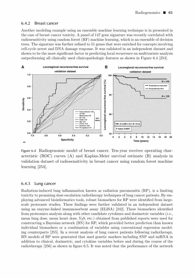
Radiogenomics � 61
6.4.2 Breast cancerAnother modeling example using an ensemble machine learning technique is in presented inthe case of breast cancer toxicity. A panel of 147 gene signature was recently correlated withradiosensitivity using random forest (RF) machine learning, which is an ensemble of decisiontrees. The signature was further refined to 51 genes that were enriched for concepts involvingcell-cycle arrest and DNA damage response. It was validated in an independent dataset andshown to be the most significant factor in predicting local recurrence on multivariate analysisoutperforming all clinically used clinicopathologic features as shown in Figure 6.4 [254].
Figure 6.4 Radiogenomic model of breast cancer. Ten-year receiver operating char-
acteristic (ROC) curves (A) and Kaplan-Meier survival estimate (B) analysis in
validation dataset of radiosensitivity in breast cancer using random forest machine
learning [254].
6.4.3 Lung cancerRadiation-induced lung inflammation known as radiation pneumonitis (RP), is a limitingtoxicity to promising dose escalation radiotherapy techniques of lung cancer patients. By em-ploying advanced bioinformatics tools, robust biomarkers for RP were identified from large-scale proteomic studies. These findings were further validated in an independent datasetusing an enzyme-linked immunosorbent assay (ELISA) [242]. These biomarkers identifiedfrom proteomics analysis along with other candidate cytokines and dosimetric variables (i.e.,mean lung dose, mean heart dose, V20, etc.) obtained from published reports were used forconstructing a Bayesian network (BN) for RP, which provided better prediction than knownindividual biomarkers or a combination of variables using conventional regression model-ing counterparts [255]. In a recent analysis of lung cancer patients following radiotherapy,BN models of RP were generated that used genetic markers including SNP and miRNA inaddition to clinical, dosimetric, and cytokine variables before and during the course of theradiotherapy [256] as shown in figure 6.5. It was noted that the performance of the network

62 � A Guide to Outcome Modeling in Radiotherapy and Oncology
improved by incorporating during treatment cytokine changes achieving an area under thereceiver-operating characteristic (ROC) curve of 0.87.
Figure 6.5 Radiogenomic model of lung cancer.An outcome model using systems bi-
ology techniques based on Bayesian networks is used for modeling radiation pneu-
monitis (RP) in lung cancer. First row shows pre-treatment BN modeling of RP.
(a) Markov blanket, (b) BN structure, and (c) ROC analysis on cross-validation.
The second row shows during-treatment BN modeling of RP. (d) Markov blanket,
(e) BN structure, and (f) ROC analysis on cross-validation [256].
6.5 CONCLUSIONSDue to advances in biotechnology, and complex biologic analysis the amount of potentialdata available for association with outcomes has grown exponentially in the past decade.This -omics revolution has provided new opportunities for re-shaping our understandingof treatment outcome response. The addition of relevant biomarkers to clinical or image-based outcomes models is likely to improve prediction performance by capturing more ofthe underlying manifestation of the pathophysiology of disease in question. However, withthis large amount of patient-specific biological information, in addition to other resourcesof data, precautions should be taken to avoid pitfalls of under- or over-fitting during thebuilding process of outcome models.

IITop-down Modeling Approaches
63

C H A P T E R 7
Analytical and mechanisticmodelingVitali Moiseenko, PhD
Jimm Grimm, PhD
James D. Murphy, PhD
David J. Carlson, PhD
Issam El Naqa, PhD
CONTENTS
7.1 Introduction . . . . . . . . . . . . . . . . . . . . . . . . . . . . . . . . . . . . . . . . . . . . . . . . . . . . . . . . . . . . . 667.2 Track structure and DNA damage . . . . . . . . . . . . . . . . . . . . . . . . . . . . . . . . . . . . . 677.3 Linear-quadratic model . . . . . . . . . . . . . . . . . . . . . . . . . . . . . . . . . . . . . . . . . . . . . . . . . 697.4 Kinetic reaction rate models . . . . . . . . . . . . . . . . . . . . . . . . . . . . . . . . . . . . . . . . . . . . 73
7.4.1 Repair-misrepair and lethal-potentially-lethal models . . . . . . . . . . 737.4.2 Refined models . . . . . . . . . . . . . . . . . . . . . . . . . . . . . . . . . . . . . . . . . . . . . . . . . . 747.4.3 The Giant LOop Binary LEsion (GLOBE) . . . . . . . . . . . . . . . . . . . . . 757.4.4 Local Effect Model (LEM) . . . . . . . . . . . . . . . . . . . . . . . . . . . . . . . . . . . . . . 757.4.5 Microdosimetric-kinetic model (MKM) . . . . . . . . . . . . . . . . . . . . . . . . . 767.4.6 The Repair-misrepair-fixation model . . . . . . . . . . . . . . . . . . . . . . . . . . . 76
7.5 Mechanistic modeling of Stereotactic Radiosurgery (SRS) andStereotactic Body Radiotherapy (SBRT) . . . . . . . . . . . . . . . . . . . . . . . . . . . . . . 777.5.1 LQ limitations and alternative models . . . . . . . . . . . . . . . . . . . . . . . . . 79
7.6 Incorporating biological data to describe and predict biologicalresponse . . . . . . . . . . . . . . . . . . . . . . . . . . . . . . . . . . . . . . . . . . . . . . . . . . . . . . . . . . . . . . . . . 81
7.7 Conclusions . . . . . . . . . . . . . . . . . . . . . . . . . . . . . . . . . . . . . . . . . . . . . . . . . . . . . . . . . . . . . 82
65

66 � A Guide to Outcome Modeling in Radiotherapy and Oncology
ABSTRACTWe provide a comprehensive review of mathematical models of cell survival following expo-sure to ionizing radiation, and their connection to clinical outcomes. We emphasize mech-anistic models which aim to account for mechanisms governing cell response to radiation.We discuss approaches to describe the process of translating primary radiation-inducedDNA damage into lethal lesions, and role of repair and binary misrepair in this process. Wedescribe reaction-rate models and models accounting for track structure and DNA organi-zation in the cell nucleus, as well as the connection between these models and the popularlinear-quadratic model. We discuss the importance of accounting for dose fractionation orprotraction by different models. We present different approaches to incorporate biologicaldata revealed by molecular and functional imaging, for example the effect of hypoxia, tomodel cell survival and tumor response. Finally, we present models specifically developed topredict cell survival and tumor response following large doses per fraction, as in intracranialstereotactic radiosurgery/radiotherapy and stereotactic body radiotherapy.
Keywords: radiation, cell survival, dose-response, linear-quadratic model, tumor controlprobability.
7.1 INTRODUCTION
MECHANISTIC models must account for our understanding of how the physical,chemical, and biologic processes lead to the endpoint under investigation. Our knowl-
edge and interpretation of how radiation-induced biological effects develop, from the atomicand cellular levels up to tumor and normal tissue response have evolved over the years.However, detailed understanding of certain steps involved in the development of radiation-induced damage, and factors mediating this process, remains limited. Despite this, mech-anistic models have been efficiently used to probe the relationships of physics, chemistryand biology over different spatial and temporal scales on integral endpoints, such as cellsurvival, normal tissue and tumor response.
While tumor and normal tissue effects are of primary interest to the radiation oncologycommunity, these tissue-level effects are mechanistically connected to underlying radiation-induced DNA damage and cell death, even though the target cell population may not bewell defined. This relationship permeates multi-scale models and provides a framework fordescribing the radiosensitivity of tumor and normal tissue in response to modifiers, suchas dose fractionation/protraction, hypoxia, radiation quality, etc. While statistical models,also known as empirical or phenomenological models, are merely designed to quantitativelydescribe observed data, mechanistic models allow us to explore the underlying biologicalcauses of observed experimental phenomena and assess the significance of specific factorsthat alter the response to radiation.
Ongoing mechanistic modeling efforts to address the complex relationship between fac-tors affecting radiation-induced cell death closely follow our understanding of underlyingphysical and biological mechanisms. Basic components of the process leading to cell kill,specifically, induction of primary lesions, repair, misrepair, dependence of radiation sensi-tivity on the phase of cell cycle, dose rate/fractionation effects, have been established sincethe early days of radiation biology. Attempts to combine these components into modelshave been a central research theme for radiobiologists and radiation physicists. Niedererand Cunningham [257] proposed a sophisticated model to describe cell survival following

Analytical and mechanistic modeling � 67
fractionated irradiation in 1976. The authors considered cell proliferation and kinetics, inparticular mitotic delay, as they mediate biological response. Notably, this early attempt toproduce a mechanistic model was made before detailed atomistic representation of DNA,Monte Carlo-generated particle tracks, binary effects in DNA misrepair, effect of chromo-some domains and other important biological phenomena which have moved to the forefrontof modeling biological effects on the DNA and cellular levels.
Many mechanistic models of cell survival aim at accounting for these various factors,including the track structure of particles, DNA organization, the complexity and spatialdistribution of DNA damage, and the relationship between these factors to DNA repair andmisrepair. Applicability of these models in the radiation therapy world, however, needs tobe rigorously tested for robustness using actual clinical data. Most models currently im-plemented in biologically-guided radiation therapy (BGRT) remain empirical. This chapterdescribes models which are not strictly mechanistic but driven by our understanding ofunderlying biophysical processes. These models will be connected to the linear-quadratic(LQ) model, which is by far the most commonly used model in the radiation oncology com-munity to describe the biological effect of radiation dose, dose per fraction, and dose ratefor radiotherapy treatments. This chapter focuses mainly on reproductive cell death (alsoknown as mitotic or proliferative), i.e., when cells die while attempting to divide. This is thedominant pathway of cell kill as it relates to modeling radiation therapy outcomes and thenarrative below applies to the typical doses and fractionations used in radiation therapy.Other pathways, for example apoptosis, are not considered in this chapter.
7.2 TRACK STRUCTURE AND DNA DAMAGERadiation-induced cell death in mammalian cells has been conclusively linked to radiation-induced DNA damage [258, 259, 260]. Cell survival models are based on concepts of primarylesions and lethal lesions, the latter resulting from primary lesions following processes de-scribed below. DNA double-strand breaks (DSB), or at least a subset of DSB, have beenidentified as the precursors which ultimately lead to formation of lethal lesions [261]. Ex-ploring the mechanisms of DNA damage induction by radiation, damage complexity as itrelates to DNA repair, and the spatial distribution of DNA lesions in the cell nucleus andamong chromosome domains are vital steps required to understand radiation-induced cellkill. Understanding these relevant mechanisms requires detailed knowledge of energy depo-sition pattern and chemical evolution of a particle track on the DNA scale.
The sequence of events leading to radiation-induced cell kill has been established, al-though our knowledge of mechanisms governing each step varies greatly between steps. Theoverall sequence and timing are outlined in Figure 7.1. Note that time scale for stages fol-lowing the pre-chemical stage are strongly dependent on cell type and repair capacity. Ina typical cellular environment, chemical evolution is complete by 108 − 107s [262]. Energydepositions by electrons and heavy charged particles are presently well understood, at leastfor energy depositions in liquid water. Monte Carlo codes to simulate energy depositionsin matter have been developed, reported, and reviewed [263, 264]. Further, track struc-ture codes have been applied to model radiation-induced damage, e.g., PARTRAC [265],NOREC [266], and GEANT4-DNA [267].

68 � A Guide to Outcome Modeling in Radiotherapy and Oncology
Figure 7.1 Sequence of events governing mammalian cell response to ionizing radia-
tion.
Monte Carlo track structure codes model energy deposition in water whereas the tar-get of interest is DNA. While modeling indirect effects requires consideration of producingionizations and excitations in water molecules, modeling direct effects has to rely on a repre-sentative model of DNA. This representation has progressed dramatically through the yearsstarting with simple geometric-volumetric approach, with DNA modeled as a cylinder struc-ture with segments assigned as bases and sugar-phosphate backbone [268]. This simplifiedrepresentation has been replaced by detailed atomistic models including hydration shells.Figure 7.2 shows the basic components required to model cellular DNA linear DNA and anucleosome including linker DNA [269, 270]. Higher levels of DNA organization have beensuccessfully modeled [265, 271] and are described in details in chapter 10. These models,

Analytical and mechanistic modeling � 69
combined with detailed track structure consideration, bridge the gap between DNA damageand chromosome aberrations, some of which are known to be lethal.
Figure 7.2 Left panel: ten-base pair segment of linear DNA (large size symbols)
including the first hydration shell (small size symbols); right panel: one nucleosome
including the linker DNA.
These models are capable of probing for impact of damage complexity, geometricaldistribution of DNA damage within and between chromosome domains, and the relationof these characteristics to radiation quality. Therefore, accounting for damage complexitywhen considering repair, or accounting for geometrical distribution of DSB when consideringformation of exchanges, can be achieved.
7.3 LINEAR-QUADRATIC MODELThe linear-quadratic (LQ) model is the most commonly used model in radiation therapy toaccount for dose fractionation/protraction, to propose and compare fractionation schedules,and to compensate for missed fractions. Broad use of this simple but versatile model owesin large part to efforts by Dr. J.F. Fowler, who pioneered the use of radiobiological modelingin radiation therapy [272]. Commonly used concepts of biologically effective dose (BED),distinguishing between early and late radiation response and how they connect to radiobi-ological parameters have been developed by Dr. Fowler and will remain in the forefront ofradiation therapy [14].
The LQ equation, in a form accounting for dose fractionation/protraction, has beenoriginally applied to describe the yield of chromosome aberrations, Y , as a function of dose,D [273]:
Y = αD +GβD2 (7.1)
Coefficients α and β describe two pathways of producing chromosome aberrations , one-track and two-track action, respectively. The Lea-Catcheside factor , G, accounts for dosefractionation/protraction, and, if we assume mono-exponential repair as a function of time:

70 � A Guide to Outcome Modeling in Radiotherapy and Oncology
G =2
D2
∫ ∞
−∞D(t)dt
∫ t
−∞e−λ(t−t′)D(t′)dt′ (7.2)
where is D is dose rate as a function of time, t, and λ is a repair constant. The linkbetween the number of chromosome aberrations and cell survival was established in the sem-inal report by Cornforth and Bedford [274], although cell survival is not solely dependenton the presence of certain types of aberrations [275]. The authors showed that the propor-tion of cells surviving and the proportion of cells free from certain types of chromosomeaberrations closely match. This implies that certain types of chromosome aberrations areindeed lethal. These chromosome aberrations are called unstable because their frequencydecreases through cell divisions as cells containing these aberrations are incapable of pro-gressing through mitosis. This is in contrast to stable chromosome aberrations, for examplesymmetric translocations, which may corrupt the genetic material but do not interfere withcell division.
Studies of dose dependence for chromosome aberrations also reveal that while certainaberrations, for example terminal deletions, show linear dose-response, other aberrationssuch as dicentrics show a pronounced quadratic term for low-LET radiation. This connectsto the binary exchange concept which is the cornerstone of the LQ model [276]. Table 7.1shows the general pathway of inducing stable and unstable chromosome aberrations. Thistable also demonstrates how the induction of chromosome aberrations, some of which arelethal, connects to the one-track/two-track foundation of the LQ model. Chromosome aber-rations shown in the fourth column of the bottom three rows require two DSBs. If eachDSB is produced by a separate track (two-track action), the frequency of these aberrationswill depend on dose squared. This also illustrates how the quadratic term in the Equation7.1 is dependent on dose rate as both DSBs have to be in the same cell at the same time,and capable of interaction, for an exchange to form.
The debate whether LQ is a mechanistic or purely empirical model has been on-goingand proponents of the model point to one-track/two-track pathways, and accounting fordose protraction/fractionation as mechanistically-based basics of the LQ formalism [275].It was pointed out that the basis of the model does not apply to large doses per fraction.Specifically, the LQ model over-predict cell lethality for doses relevant to stereotactic ra-diosurgery (SRS) and body radiotherapy (SBRT) [277]. Counter-arguments question thevery foundation of the model from both microdosimetric and statistical point of view [278].Despite limitations on the model, it remains the current standard model used in radiationoncology, in particular when it comes to isoeffect calculations [14]. The basic equation con-necting cell survival and tumor control probability (TCP) based on Poisson statistics is[279]:
S = e−αD−GβD2
(7.3)
TCP = e−NS = e−N0S = e−Noexp(−αD−GβD2) (7.4)
where NS is the number of surviving tumor cells capable of regrowing the tumor (clono-gens) , N0 is the initial number of clonogens, and S is the surviving fraction. For a specificcase of fractionated treatment with dose D delivered in n fractions we can assume thattime to deliver a fraction is too short for repair to impact the quadratic term, i.e., whenaccounting for intra-fraction dose-rate effects G = 1. Time between fractions is typically

Analytical and mechanistic modeling � 71
TABLE 7.1 Example of outcomes following induction and repair/misrepair of DNA DSBs. Faithfulrestitution means that the cell is viable. Failure to repair makes the cell non-viable. Binary eventsmay leave the cell viable (third column) or result in chromosome aberrations which lead to celldeath, although not necessarily in the first division (fourth column).

72 � A Guide to Outcome Modeling in Radiotherapy and Oncology
sufficient for full repair to preclude interactions between lesions produced by different frac-tions, i.e., for inter-fraction effects G = 0, overall value of the Lea-Catcheside factor is wellapproximated by G = 1/n. To further account for tumor cell proliferation after a lag periodof TK :
TCP = e−NS = e−N0S = e−Noexp(−αD−βdD+γ(T−TK)) (7.5)
where d is dose per fraction D/n, T is overall treatment time, and γ is the repopulationterm γ = ln2/Tp, where Tp is the doubling time for tumor clonogens. Lag period, TK , wasestimated at four weeks for head and neck and lung cancer [163, 280]. The repopulationterm only apples for T > TK . This formulation is obviously simplified. At minimum thesesimplifications assume that there is no inter-patient variability in cell radiosensitivity orinitial number of clonogens in a tumor, all cells within a tumor are equally sensitive, anddose is uniform through the tumor volume.
Accounting for different sources of heterogeneity will require additional model parame-ters, which is highly undesirable. Moreover, there is reciprocity in heterogeneity, for examplemathematically increasing the initial number of clonogens can be compensated by assumingradioresistance. This is clearly demonstrated by the inter-patient heterogeneity model pro-posed by Webb and Nahum [281]. The authors suggested ignoring the quadratic term in theLQ equation, then, accounting for inter-patient heterogeneity with the following equation:
TCPIPH =
∫ψ(α, α, σα)e
−N0exp(−αD)dα (7.6)
where ψ describes the distribution of α among patients, this distribution is often assumedGaussian, with the mean value α and standard deviation σα. This equation clearly showshow variation in the number of clonogens and variation in α can be re-cast mathematically.For any arbitrary dose distribution and clonogen density distribution we can divide thevolume into voxels small enough so that dose and clonogen density are uniform. Then theoverall TCP is dependent on the product of voxel control probabilities, VCP. If voxel ireceives dose Di, there are Ni clonogens in the voxel i, and there are M voxels the aboveequation can be generalized:
TCPIPH =
∫ψ(α, α, σα)
M∏i=1
V CPidα =
∫ψ(α, α, σα)
M∏i=1
e−Niexp(−αDi)dα (7.7)
This equation is generic and for practical applications has to be connected to realisticdistributions. Moreover, use of functional imaging to probe for properties affecting radio-therapy outcome, has been growing. Accounting for these properties is shown in Section 7.5.
The LQ expression can be derived using multiple methods including detailed reaction-rate models as shown in Section 7.4, or a premise which bypasses mechanistic considerations.Specifically, the theory of dual radiation action [282] connects biological response of a cell asa second order reaction of sublesions, and the number of radiation-induced sublesions in asensitive volume proportional to a microdosimetric quantity, specific energy, z. Assumptionof binary interactions is again at the core of the formulation. For a dose D, the number oflesions, E(D), which result from sublesions, is:
E(D) = K(zD +D)D (7.8)

Analytical and mechanistic modeling � 73
where zD is dose-mean specific energy and K is a constant characteristic of a cell. At lowdoses when the quadratic term can be ignored this model gives a simple microdosimetricallydriven method to calculate RBE, which is simply a ratio of dose-mean specific energy values.This formalism also implies that the quadratic term is cell-line specific, and is not connectedto microdosimetric quantities.
7.4 KINETIC REACTION RATE MODELSThe LQ model, while providing a versatile formalism to account for time-dose-fractionation,in particular for isoeffect calculations, does not explicitly describe the production of pri-mary lesions (DSB), their repair and misrepair, and the production of lethal lesions. Thekinetic reaction rate model describes the processes of the production of primary lesions andtheir processing using equations of chemical kinetics, hence the name kinetic. The repair-misrepair (RMR) and lethal-potentially-lethal (LPL) models [283, 284] formulated in themid 1980s serve as a benchmark. These two models contained binary exchanges as a pathwayof lethal lesion production which has become an integral feature of refined models. Overall,reaction rate models follow the pathways outlined in table 7.1, at least as far as binaryexchanges are concerned [285]. Notably, interpretation of the events which downstream leadto the linear term in dose-response remains uncertain. Although our knowledge of DNAdamage, repair mechanisms and pathways of cell lethality are much more advanced com-pared to the 1980s, we still know more about behavior of the linear term, α, as a function ofradiation quality, and how it varies between cell lines, rather than how it comes about [286].
It is well established that as dose rate decreases the contribution of the quadratic termto cell death also decreases, while the α term remains unchanged; that is, unless doserate becomes ultra-low and other factors like repopulation or reassortment start playinga role. An interpretation of events leading to a terminal deletion, Table 7.1, varies frommodel to model, including in the RMR and LPL. While some models assume conversionof sublethal lesions into lethal lesions via lethal restitution [284], others assume that aproportion of sublethal lesions fail to go through either repair or misrepair pathway andtherefore remain as residual by the time a cell reaches mitosis [287]. Other alternative modelshave been proposed and extensively reviewed [285]. The LPL model makes a considerablydifferent assumption in that it proposes a pathway of direct production of a lethal lesionby a single track. This difference, while appearing minor, leads to different formalism forlethal lesion production. In RMR, a certain proportion of sublethal lesions is converted intolethal lesions via lethal restitution, and at any time is dependent on the number of sublethallesions present and rate of lethal restitution [284]. Conversely, in the LPL model the rate ofproducing single-track lesions will be proportional to dose rate [283]. Most notably, underspecific circumstances the solution to the reaction rate models reduces to the LQ equation[285].
7.4.1 Repair-misrepair and lethal-potentially-lethal modelsThese models have been extensively reviewed in the literature though only a brief descriptionis presented in this chapter. The RMR model is based on the pathways outlined in Table7.1 and assumes existence of uncommitted lesions. The productions of these lesions (e.g., aDSB) is linearly correlated with dose, their repair is assumed mono-exponential, and binarymisrepair pathways of lethal lesion production is an important feature of this model [284].

74 � A Guide to Outcome Modeling in Radiotherapy and Oncology
The equations describing the rate of producing primary lesions, U , their repair, misrepairand production of lethal lesions, L [285]:
dU
dt= δD − λU − kU2 (7.9)
dL
dt= (1− ϕ)λU + (1− ψ)kU2 (7.10)
Primary lesions are produced with a rate δ, repaired with a time constant λ, and binarymisrepair occurs at a rate k. A certain proportion of repair (1-φ) leads to lethal restitutionand a proportion of binary exchanges (1-ψ) are lethal. Assuming that the Poisson statisticsapplies the surviving fraction is simply the exponent exp(−L(t)). For certain simple initialconditions the solution is possible, in particular for a situation relevant to radiation therapy,when full dose is delivered in a period of time too short for repair to take place, and fullrepair is allowed.
Sachs et al. [285] argued that (1-ψ)=1/4, which, as illustrated in Table 7.1 means thatfor one dicentric we need four DSBs because a dicentric results from 2 DSBs half of thetime, the other half results in a symmetric translocation. Then, following the narrative ofSachs et al, if repair dominates misrepair, kU2 << λU , and repair/misrepair are allowed torun full course, which is to say we can justify setting time to infinity, the solution reducedto LQ. Equation 7.3 can therefore be obtained under these assumptions and:
α = δ (1− ϕ) (7.11)
β =(ϕ− ψ) kδ2
2λ(7.12)
The LPL model assumes presence of potentially lethal lesions, nPL, with their productionand repair/binary misrepair identical to shown above for RMR. However, this model isdistinctly different from RMR in describing production of lethal lesions, L. As discussedabove it assumes a direct one-track production of lethal lesions [283], consequently:
dL
dt= αD + ckn2
PL (7.13)
While these models are different in their formulation, notably, the solutions can-be recastfrom one model to another [285].
7.4.2 Refined modelsAs any other model, RMR and LPL models are based on assumptions and as our knowl-edge of events leading to radiation-induced cell kill progresses these assumptions change.Two aspects of the RMR and LPL models are in particular simplifications and these havebeen addressed in refined models. First, both models disregard DNA organization in thecell nucleus. While DSB yield is known to linearly depend on dose at least in the doseregion of interest for radiation therapy, yield of lethal lesions and frequency of chromo-some aberrations are non-linear functions of dose. This conversion of linear to non-linearhas been conclusively attributed to repair/misrepair, and in particular binary events [288].Ideally, modeling of events leading to cell lethality should to account for track structureand how this track structure interplays with DNA organization. The latter concept hasreceived plenty of attention in the literature with chromatin fiber, loops, and chromosome

Analytical and mechanistic modeling � 75
domain organization in interphase modeled in fine detail [289, 290, 291]. Second, both mod-els assume exponential repair, which is a simplification [292]. In addition to the presenceof repair pathways characterized by different time constants [286], e.g., slow and fast repair[293], other aspects of repair behavior as a function of time and dose have been addressed,for example repair saturation [294].
Attention to track structure and its interplay with DNA organization was in partprompted by increased interest in proton therapy, and investments in carbon ion radio-therapy. It has been long accepted that not all DSBs are created equal and accompanyingstrand breaks or base damage contribute to their complexity, prompting researchers to des-ignate complex DSB as DSB+ or DSB++ [295]. Another hypothesis is that these DSBmay present a stronger challenge to repair enzymes [296] and may be prone to misrepair[297]. The question of radiation quality is then not only if high-LET radiation produces moreDSB per unit dose compared to X- or γ-rays, but also if these DSB are functionally different[298, 299]. This, combined with track structure-driven proximity effects, i.e., spatial distri-bution between DSB and their distribution in fiber, loops and domains, are pre-requisite tomechanistically address effects of radiation quality on cell kill [300, 289, 301]. Some of theserefined models are briefly described below.
7.4.3 The Giant LOop Binary LEsion (GLOBE)The Giant LOop Binary LEsion (GLOBE) model [291] accounts for DNA organizationand is motivated by the concept of chromatin loops approximately 2 Megabasepair in size.The model distinguishes between isolated DSB within a loop iDSB and clustered damageproducing multiple DSB in one giant loop, cDSB. Cell survival is assumed to obey thePoisson distribution, that is, the exponent to the expectation value for the number of lethallesions is equal to survival probability. Spatial-temporal production of DSB can then beconverted into survival:
S = exp(−εini − εcnc) (7.14)
where ni and nc are expectation values for iDSB and cDSB, and εini + εcnc is theexpectation value for the number of lethal lesions. The model allows for binary exchangesbetween DSB produced in different domains, however does not account for correlation ofthe number of DSB in proximal loops. This model has been applied to describe cell survivaldata for photons including ultra-soft photons, and comparisons with RMR and LPL modelshave been presented [291, 302, 286]. Notably, the authors demonstrated that until doseis large (tentatively >10 Gy, however exact value is cell line-dependent), LQ and GLOBEmodels agree in their predictions and LQ parameters can be re-cast from the GLOBE modelparameters [303].
7.4.4 Local Effect Model (LEM)To specifically address modeling of cell survival to serve as a radiobiological foundation forion beam therapy a model tailored to account for the energy deposition pattern charac-teristic of ion beam was proposed. The Local Effect Model (LEM), which went through anumber of updates (LEMI-LEMIV) in an attempt to account for energy deposition patternthrough the concept of local dose. The premise of the LEM is that microscopic local dosedistribution pattern determines biological effect, and equal local doses lead to equal localeffects, irrespective of radiation quality. This model has been put forward to account for spa-

76 � A Guide to Outcome Modeling in Radiotherapy and Oncology
tially correlated distribution of DSB following traversal of a cell nucleus by a heavy chargedparticle. This pattern of producing correlated DSB within a single loop may further lead torelease of DNA segments not attached to the nuclear matrix [291, 304]. The mean numberof DSB in a subvolume is derived from photon data, showing a yield of approximately 30DSB per cell per Gy. From a local average number of DSB, the spatial distribution of DSBis calculated using Monte Carlo simulations amorphous track structure pattern in placeof the probability density function of DSB. Indirect effects, i.e., DNA damage by radicalsfollowing water radiolysis, are accounted for in LEM by smearing radial dose profile. Theauthors propose use of a cluster-index:
C =NcDSB
NcDSB +NiDSB(7.15)
where NcDSB and NiDSB are numbers of loops containing clustered and isolated DSB.This index quantitatively captures the effect of clustering as heavy ions will be likely todeposit energy locally and produce correlated breaks within a loop. The model has beendemonstrated to accurately describe the RBE dependence on LET for V79 cells [291].
7.4.5 Microdosimetric-kinetic model (MKM)The microdosimetric-kinetic model (MKM) builds on microdosimetric concepts whichserved as a foundation of the dual radiation action theory [282]. Similar to LPL and RMR,MKM describes production of potentially lethal lesions and their processing into lethal le-sions as differential equations [305, 306, 307, 308]. The basic premise of the MKM is that thecell nucleus is divided into equal size compartments (or domains) which fill the volume of anucleus like a jigsaw puzzle and their number can be from a few hundred to a few thousand.If reshaped into spheres these domains will have a diameter of 0.5-1 μm. Equal size doesnot imply equal DNA mass, which is allowed to vary between domains. A radiation-inducedDNA lesion is confined to a domain and interactions between lesions in different domainsis not allowed. Dose variation from domain-to-domain is accounted for to mimic a traversalof the cell nucleus by a charged particle. Similar to RMR or LPL, potentially lethal lesionscan undergo faithful restitution, conversion to a lethal lesion and binary exchanges confinedto a domain. The MKM model has been used to predict RBE as a function of LET and aconnection to LQ parameters, suitable for RBE analysis has been reported [307].
7.4.6 The Repair-misrepair-fixation modelAs DSB are the most critical form of initial DNA damage formed by radiation, it is con-ceptually appealing to link trends in the α and β parameters of the LQ model with particletype and LET to DSB induction. The Repair-Misrepair-Fixation (RMF) model directlylinks DSB induction and processing to clonogenic cell death [309]. In the RMF, a coupledsystem of non-linear ordinary differential equations is used to model the time-dependentkinetics of DSB induction, rejoining, and pairwise DSB interaction to form lethal (and non-lethal) chromosomal damage. The RMF model assumes that it is the formation of lethalpoint mutations and chromosome damage rather than the initial DSB themselves that arethe dominant mechanism underlying the effects of particle LET on cell death. Earlier ki-netic reaction-rate models such as the RMR and LPL models also assume both linear andquadratic terms for the repair of sub-lethal and potentially lethal damage. However, in theRMF model, the initial formation of DSB is assumed to follow a compound Poisson processinstead of a simple Poisson process as in the RMR and LPL models. Reproductive cell deathby mitotic catastrophe, apoptosis, or other cell death modes are explicitly linked to DSB

Analytical and mechanistic modeling � 77
induction and processing in the RMF model. Table 7.1 shows all potential DSB processingpathways. The effect of radiation quality q on the α and β radiosensitivity parameters ofthe LQ model can be effectively modeled using [309, 310, 311]:
α (q) = θΣ(q) + kzF (q)Σ2(q), (7.16)
and
β (q) = (k/2)Σ2(q) (7.17)
Here, Σ is the initial number of DSB per Gray per giga base pair (Gy−1 Gbp−1), zF is thefrequency-mean specific energy (Gy), and θ and κ are tumor- or tissue-specific parametersrelated to the biological processing of initial DSB into more lethal forms of damage (e.g.,chromosome aberrations). θ is the fraction of DSB that undergo lethal first-order misrepairand damage fixation, whereas κ is the fraction of initial DSB that undergo pairwise damageinteraction. An attractive feature of Equations 7.16 and 7.17 is that estimates of α and β forany particle type, including electrons and photons, are determined by a well-defined, purelyphysical parameter that is the same in vitro and in vivo (zF ), two biological parameters (θand κ) that are tissue-specific but independent or a weak function of radiation quality, and abiological parameter (Σ) that is a strong function of radiation quality (track structure) butis approximately the same in vitro and in vivo and among all mammalian cells. Sophisticatedstochastic models, such as the Monte Carlo Damage Simulation (MCDS), are also availableto predict trends in Σ with radiation quality (e.g., [312, 313], and references therein).
For a reference radiation x with known radiation sensitivity parameters αx and βx, theradiation quality-dependent LQ parameters can also be expressed by:
α (q) =Σ(q)
Σx
(αx + 2
βx
Σx(Σ (q) zF (q)− ΣxzF,x)
), (7.18)
and
β (q) =
(Σ(q)
Σx
)2
βx (7.19)
Equations 7.18 and 7.19 provide a convenient formalism to relate published radiosensitiv-ity parameters for photons and other radiations with low-LET to radiosensitivity parametersfor other particle types, including protons and other heavier ions. It has been demonstrated[310, 311, 314] how mechanistic models, such as the RMF, can be used in particle therapy topredict the relative biological effectiveness (RBE) of heavy ions and optimize radiotherapytreatments using protons, helium, and carbon ions. This is discussed in Chapter 14.
7.5 MECHANISTIC MODELING OF STEREOTACTIC RADIOSURGERY (SRS)AND STEREOTACTIC BODY RADIOTHERAPY (SBRT)
SRS and Stereotactic radiotherapy (SRT) are special cases of extreme hypofractionationand refer to stereotactic radiosurgery in single-fraction or multiple fractions of irradia-tion for treating intracranial lesions with a very high degree of dose conformity. This ap-proach has been recently extended to extracranial radiosurgery and is often referred to asstereotactic body radiation therapy (SBRT) or stereotactic ablative radiotherapy (SABR)in the literature. It should be noted that available in vitro data mainly support appli-cation of the standard LQ model in the range of 1-5 Gy [315], and above this range iscurrently a subject of intense debate in the literature. This includes application to SRS and

78 � A Guide to Outcome Modeling in Radiotherapy and Oncology
SBRT/SABR, which typically apply higher dose per fraction than 5 Gy as discussed below[316, 317, 318, 319, 320, 321].
There are currently two schools of thought on the current clinical success of SRS/SBRTtreatments. One argument is that classic radiobiology principles (5Rs) and the LQ modelare adequate to explain the effects of large dose per fractions and the main observed advan-tages are mainly attributed to the “Geometrical Window of Opportunity” that is expandedby advancements in image-guidance and treatment delivery techniques [322, 316, 320, 321].Others highlight potential limitations of the LQ model for accurately describing high doseper fraction data and laboratory evidence suggesting the possible existence of radiobiologythat may involve new mechanisms related to stem cells, vascular damage, and immune-mediated effects or combination of these [317, 319].
Classical radiobiology principles suggest that cancers with low α/β (e.g., melanoma, li-posarcoma, prostate and some breast cancers) will benefit from hypofractionation regimenswhile typical cancers with high α/β (i.e., around 10 Gy or higher), will benefit from conven-tional or hyperfractionated regimens in terms of sparing late-reacting normal tissue. Theseeffects could be adequately discerned from the LQ model. However, application of theseconcepts to higher doses per fraction have been questioned in the light of recent SBRTresults such as RTOG-0236, which is a phase II multi-institutional trial of early stage lungcancer patients with a prescription dose of 18 Gy per fraction x 3 (54 Gy total), whichyielded an estimated 3-year primary tumor control rate of 97.6% (95% CI: 84.3%-99.7%),disease-free survival of 48.3% (95% CI, 34.4%-60.8%), and overall survival of 55.8% (95%CI, 41.6%-67.9%) [323]. These results represent remarkable improvement over conventionalfractionation, which in theory according to the LQ model would be the fractionation ofchoice for lung cancer given its high α/β.
Proponents of a unique high-dose biology cite that under certain SRS and SBRT regi-mens classical radiobiology fails to explain outcomes. For instance, SRS or SBRT deliveryfor each session is relatively longer than conventional fractionation allowing for higher ratesof sub-lethal damage SLD repair, where a fraction delivery in excess of 30 minutes may leadto loss of BED [324]. Moreover, at large doses (e.g., > 10 Gy/fraction), enhanced vasculardamage may occur [325], leading to tumor microenvironment hypoxia and acidification,which prevent reoxygenation. High doses prevent cell cycle progression and cells undergointerphase death in the cell cycle phases where they are irradiated rather than being re-distributed. Repopulation during the shortened 1-2 weeks period may be as well negligible.Furthermore, they assert that the LQ model may not be appropriate at the high doses perfraction encountered in SRS/SBRT because it was derived largely from in vitro, rather thanin vivo data, and thus does not consider the impact of ionizing radiation on the supportingtissues nor does it consider the impact of the subpopulation of radioresistant clonogens (i.e.,cancer stem-cell) or vascular damage [317, 319, 325]. On the other hand, the clinical rele-vance of these unique high-dose biological mechanisms remains to be determined. The otherschool of thought argue that the 5Rs and the LQ model are supported by available preclini-cal and clinical data and there is little evidence to suggest otherwise [322, 316, 320, 321]. Forinstance, in the case of lung cancer, Brown et al. suggest that dose escalation (BED > 100Gy), rather than new biology may be adequate to explain the excellent clinical efficacy ofSBRT in early stage non-small cell lung cancer (NSCLC) patients as shown in Figure 7.3[320]. This issue is still a subject of ongoing debate given the uncertainties in the existingpublished data.

Analytical and mechanistic modeling � 79
Figure 7.3 TCP as a function of BED [320].
7.5.1 LQ limitations and alternative modelsIt is recognized that the LQ is an approximation to more sophisticated kinetic reactionmodels [283, 284], see Section 7.4. Therefore, several modifications have been introducedto the LQ model to allow better fit to high doses per fraction. These modifications to theLQ model effectively aim to straighten the survival curve at high doses, where it fails. Thiscould be achieved by simply having higher α/β values in cases of rapidly proliferating andhypoxic tumors [316, 326] or by developing alternate models to the standard LQ modelsuch as the linear-quadratic-linear (LQL) [327, 328], linear-quadratic-cubic (LQC) [329],the universal survival curve (USC) [330], and the generalized LQ (gLQ) (Wang et al. 2010)among others. Below, we briefly discuss some of these alternate LQ models intended forhypofractionation regimens.
The phenomenological Modified LQ or its equivalent kinetic LQL model modify thestandard LQ by including an additional parameter (δ), which characterizes the bending ofthe isoeffect curve at higher doses replacing the standard protraction factor of Equation 7.2as follows [327, 328]:
S = e−αD−βG(δD)D2
(7.20)
G =2
(δD)2(e−δD + δD − 1), (7.21)
where δ can vary from 0.04 to 0.4 Gy−1. In this case, G(δD) term increases survival foran acute dose fraction and supposedly accounts for the reduction in repairable lesions dueto interactions with forming lesions [327].
The LQC accounts for the linear response at higher doses by adding a term proportionalto the cube of the dose:
S = e−αD−βD2+gD3
(7.22)

80 � A Guide to Outcome Modeling in Radiotherapy and Oncology
where g = β/(3DL) and DL = 18 Gy at which the survival curve is presumed to becomea straight line.
The USC model creates a hybrid between the LQ model and the classical multi-targetmodel [330]:
lnS =
(−n(αd+ βd2
), d ≤ DT
−n(
dD0
− Dq
D0
), d ≥ DT
)(7.23)
where the transition dose (DT ), is given by DT = 2Dq/(1 − αD0). In this case, it isassumed that the LQ model gives a good description for conventional fractionation (i.e., theshoulder effect), while for ablative doses beyond the shoulder, the survival curve is betterdescribed as a straight line as predicted by the multi-target model.
The gLQ aims to continuously encompass the entire range of possible dose deliverypatterns [331]:
S = e−αD−GβD2
(7.24)
G =2
D2
n∑i=1
{R2i
ε2i(εiTi − 1 + exp(εiTi))+
i−1∑j=1
RiRjexp(−βDij)
εiεj[exp(εjtj)− exp(εjtj−1)][exp(−εiti−1)− exp(εiti)]}
(7.25)
where β2 is the second hit component of β = β1β2/2, and the dose rate pattern is givenby R(t) = Ri, ti−1 < t ≤ ti, 1 = 1, . . . , N .
It should be noted that an abundance of caution should be used when interpreting andapplying these models to clinical data and comparing their performances in terms of theassumed parameters, dose prescription, isodose lines, and the size of irradiated volume.Empirical or semi-empirical modifications to the LQ model are attempts to straighten cellsurvival response (on a log scale) at high doses [327, 328, 330, 332]. However, the un-derlying biological mechanisms implied in these modifications are often unclear and thequestion remains whether the addition of unsubstantiated parameters into the modelingprocess could help improve the predictions of clinical outcomes than the standard LQ with-out further validation. For fractionated stereotactic body radiation therapy (SBRT), severalinvestigators found that the standard LQ model suffices when modeling local tumor control[333, 334, 316, 321] and pulmonary toxicity [335, 336]. Alternative high-dose models didnot provide better fits of the clinical data than the two-parameter LQ model. Mehta et al.[337] found that when analyzing the available clinical data for early-stage non-small celllung cancer (NSCLC), the clinical significance between the LQ and USC models at thera-peutic doses in an SBRT regimen is minimal. A recent analysis of the available local controldata for 3,000 early-stage NSCLC and brain metastases patients undergoing single- andmulti-fraction SBRT found that the LQ model with heterogeneous radiosensitivity provideda significantly better fit over the entire range of treatment doses than did any of the high-dose alternative models [321].
The analysis of published local control data for lung tumors and brain metastases frompatients undergoing stereotactic radiotherapy suggests that unique tumoricidal mechanisms
Analytical and mechanistic modeling � 81
do not determine tumor control at high doses per fraction[320, 316, 321]. However, morehomogeneous clinical data sets are needed to further test this hypothesis. In addition, thenegative impact of tumor hypoxia on biological effectiveness may be more significant in thecontext of hypofractionation [316, 338], particularly for single-fraction SBRT [333, 334, 321].
7.6 INCORPORATING BIOLOGICAL DATA TO DESCRIBE AND PREDICT BI-OLOGICAL RESPONSE
Biological imaging, specifically molecular and functional imaging, provides a means to probetumor and normal tissue properties which may impact response to radiation. The mostcommonly used modalities including positron emission tomography (PET), single photonemission tomography (SPECT) and functional magnetic resonance imaging (fMRI) providequantitative tools to assess spatial distribution of a property of choice for an individual pa-tient, a field currently known as radiomics (see Chapter 3). These properties include glucosemetabolism, hypoxia, perfusion, diffusion, cell proliferation, membrane synthesis and aminoacid metabolism. Emphasis thus far has been on probing tumor properties and designingtrials to account for tumor biology. There is convincing evidence that select properties suchas hypoxia or metabolic activity assessed by biological imaging before or during the courseof radiotherapy relate to outcomes. In particular, a relationship between tumor control andtumor biological properties was demonstrated for non-small lung cancer [339], rectal cancer[340], and cervical cancer [341]. Boosting the dose to regions which show properties associ-ated with higher risk recurrence, e.g., large concentration of tumor cells, hypoxia or rapidproliferation, is an intuitive yet clinically unproven approach to individualize radiotherapytreatments for specific subgroups of patients. Designing these boost targets ideally shouldrely on dose-response and a mechanistic understanding of how a particular property affectsthis response.
Segmenting the regions for boosting and designing discrete levels for dose boosts repre-sents an inviting method to enhance radiotherapy planning because tools readily availablein commercial treatment planning systems can be used [342]. This is a practical take on thedose painting-by-numbers approach [343]. The biggest obstacles in utilizing this approachare that the desired dose must be connected to the specific property, and this relationship, aswell as the quantitative relationship between biological imaging and actual property, remainuncertain. The simplest approach to design boost doses connected to a property, which isdescribed by a voxel intensity, I, is to assume a linear relationship between dose and in-tensity, under constraints that there is a minimum baseline dose required, Dmin, and thereis maximum dose to ensure safe radiotherapy, Dmax. This leads to a simple relationshipbetween dose and voxel intensity:
D (I) = Dmin +I − Imin
Imax − Imin(Dmax −Dmin) . (7.26)
This formalism is void of any relationship between biological imaging and modificationof response. The LQ equation based on Poisson statistics, Equation 7.3, is versatile and canreadily accommodate factors affecting outcomes. Depending on the nature of the factor thiscan be incorporated either through modifying dose-response characteristics, or weight of avoxel. In the simplest case of non-uniform spatial distribution of tumor cells the number ofsurviving cells can be rewritten as:
Ns =∑
viρiSi (7.27)

82 � A Guide to Outcome Modeling in Radiotherapy and Oncology
where ρi is cell density and vi is fractional volume. Factors which modify dose-responsehave to cast through LQ model parameters. Hypoxia in particular received attention asuse of PET and MRI to probe for hypoxia has been expanding [344, 345]. Modeling effortshave concentrated on accounting for hypoxia through well-established modifying factors,e.g., oxygen enhancement ratio (OER), focusing on deriving OER estimated from in vitroand in vivo data [346], including the effects of intermediate levels of hypoxia on treatmentresponse for different dose fractionations [338, 347], and separating the effects of chronicand acute hypoxia. Preclinical studies have demonstrated promise, for example, a modelwas developed and tested on a rat sarcoma data set [348]. The premise of the approach isto modify LQ parameters, α and β, established for oxygenated conditions to account forpresence of hypoxia, for example for chronic hypoxia LQ parameters αch and βch:
OERch =α0
αch=
(β0
βch
)(1/2)
(7.28)
Surviving fraction for fractional dose d then:
S = e−αd
OERch− βd2
OER2ch (7.29)
Accounting for acute hypoxia can be done in a similar manner except acute hypoxia,by definition is present only a portion of the time. The model has been further translatedfrom applying to preclinical studies to predicting TCP for NSCLC following SBRT. Pres-ence of hypoxia may be an important factor in hypofractionated treatment [349] because ofreduced potential for reoxygenation compared to conventional fractionation [338]. Owing tothe versatility of the Poisson-based TCP model tumor characteristics revealed by biologicalimaging, for example the presence of a quickly proliferating pools of cells can be incorpo-rated [348, 350]. As a result modeling-based optimal fractionation can be derived [351].
A compartment approach has also been tested to attempt a more sophisticated mod-eling approach [352]. The authors accounted for the interplay between proliferation andthe presence of hypoxia. Three compartments were assumed to be present: proliferative,intermediate, and hypoxic. This formalism is sophisticated and includes both radiation-induced effects, and effects caused by environmental factors, for example cell loss due tolack of access to nutrients. The model allows for cells migrating between compartments,and accounts for hypoxia and proliferation. The authors connect the model to biologicalimaging, in particular FDG-PET and investigate response modulation by different FDGprofiles [353, 352].
7.7 CONCLUSIONSMathematical models of cell survival, tumor and normal tissue response to radiation aremeant to describe observed data and make predictions for doses and fractionation schedulesconsidered for clinical practice and clinical trials. These models help assessing changes inbiological response, particularly in the absence of clinical data. The impact of these predic-tive models is particularly important in the modern radiation era which allows conformaldelivery of radiation to the tumor and boosting doses to subvolumes showing higher riskof recurrence. Mechanistic models are most appropriate for this purpose compared to em-pirical models as they rely on quantitative interpretation of mechanisms governing cell,tumor and normal tissue response to radiation. The models presented in this chapter canbe used to guide selection of new or alternate radiotherapy regimens. It is important to

Analytical and mechanistic modeling � 83
remember that uncertainties in model predictions relate to uncertainties in radiosensitiv-ity parameter estimates. These uncertainties will have a large impact on calculated doseprescriptions when the alternate treatment differs greatly from the established therapy reg-imens such as when converting standard fractionated regimens to the high dose per fractionused with stereotactic radiation. It is therefore prudent to make small incremental changesaway from conventional regimens instead of drastic changes to reduce the possibility ofmis-estimation. Ultimately, clinical data from prospective randomized trials are the goldstandard in medicine, and mathematical models, in particular mechanistic models, can onlyassist guiding clinical radiation oncology.

C H A P T E R 8
Data driven approaches I:conventional statisticalinference methods,including linear and logisticregressionTiziana Rancati
Claudio Fiorino
CONTENTS
8.1 What is a regression . . . . . . . . . . . . . . . . . . . . . . . . . . . . . . . . . . . . . . . . . . . . . . . . . . . . 868.2 Linear regression . . . . . . . . . . . . . . . . . . . . . . . . . . . . . . . . . . . . . . . . . . . . . . . . . . . . . . . . 87
8.2.1 Mathematical formalism . . . . . . . . . . . . . . . . . . . . . . . . . . . . . . . . . . . . . . . . 888.2.2 Estimation of regression coefficients . . . . . . . . . . . . . . . . . . . . . . . . . . . . 888.2.3 Accuracy of coefficient estimates . . . . . . . . . . . . . . . . . . . . . . . . . . . . . . . 898.2.4 Rejecting the null hypothesis . . . . . . . . . . . . . . . . . . . . . . . . . . . . . . . . . . . 898.2.5 Accuracy of the model . . . . . . . . . . . . . . . . . . . . . . . . . . . . . . . . . . . . . . . . . . 908.2.6 Qualitative predictors . . . . . . . . . . . . . . . . . . . . . . . . . . . . . . . . . . . . . . . . . . . 918.2.7 Including interactions between variables . . . . . . . . . . . . . . . . . . . . . . . 928.2.8 Linear regression: example . . . . . . . . . . . . . . . . . . . . . . . . . . . . . . . . . . . . . 93
8.3 Logistic regression . . . . . . . . . . . . . . . . . . . . . . . . . . . . . . . . . . . . . . . . . . . . . . . . . . . . . . 1018.3.1 Modelling of qualitative (binary) response . . . . . . . . . . . . . . . . . . . . . 1018.3.2 Mathematical formalism . . . . . . . . . . . . . . . . . . . . . . . . . . . . . . . . . . . . . . . . 1038.3.3 Estimation of regression coefficients . . . . . . . . . . . . . . . . . . . . . . . . . . . . 1058.3.4 Accuracy of coefficient estimates . . . . . . . . . . . . . . . . . . . . . . . . . . . . . . . 1058.3.5 Rejecting the null hypothesis, testing the significance of a
model . . . . . . . . . . . . . . . . . . . . . . . . . . . . . . . . . . . . . . . . . . . . . . . . . . . . . . . . . . . . 1068.3.6 Accuracy of the model . . . . . . . . . . . . . . . . . . . . . . . . . . . . . . . . . . . . . . . . . . 1068.3.7 Qualitative predictors . . . . . . . . . . . . . . . . . . . . . . . . . . . . . . . . . . . . . . . . . . . 1088.3.8 Including interaction between variables . . . . . . . . . . . . . . . . . . . . . . . . 1088.3.9 Statistical power for reliable predictions . . . . . . . . . . . . . . . . . . . . . . . . 108
85

86 � A Guide to Outcome Modeling in Radiotherapy and Oncology
8.3.10 Time consideration . . . . . . . . . . . . . . . . . . . . . . . . . . . . . . . . . . . . . . . . . . . . . . 1098.4 Model Validation . . . . . . . . . . . . . . . . . . . . . . . . . . . . . . . . . . . . . . . . . . . . . . . . . . . . . . . 109
8.4.1 Apparent validation . . . . . . . . . . . . . . . . . . . . . . . . . . . . . . . . . . . . . . . . . . . . . 1118.4.2 Internal validation . . . . . . . . . . . . . . . . . . . . . . . . . . . . . . . . . . . . . . . . . . . . . . 1118.4.3 External validation . . . . . . . . . . . . . . . . . . . . . . . . . . . . . . . . . . . . . . . . . . . . . . 112
8.5 Evaluation of an extended model . . . . . . . . . . . . . . . . . . . . . . . . . . . . . . . . . . . . . . . 1138.6 Feature selection . . . . . . . . . . . . . . . . . . . . . . . . . . . . . . . . . . . . . . . . . . . . . . . . . . . . . . . . 113
8.6.1 Classical approaches . . . . . . . . . . . . . . . . . . . . . . . . . . . . . . . . . . . . . . . . . . . . 1148.6.2 Shrinking and regularization methods: LASSO . . . . . . . . . . . . . . . . 1158.6.3 Bootstrap methods . . . . . . . . . . . . . . . . . . . . . . . . . . . . . . . . . . . . . . . . . . . . . . 1168.6.4 Logistic regression: example . . . . . . . . . . . . . . . . . . . . . . . . . . . . . . . . . . . . 118
8.7 Conclusions . . . . . . . . . . . . . . . . . . . . . . . . . . . . . . . . . . . . . . . . . . . . . . . . . . . . . . . . . . . . . 127
ABSTRACTMultivariable methods of statistical analysis are commonly used in oncology. This typeof analysis considers multiple variables to predict a single outcome, with multivariablemethods exploring the relation between two or more predictors (independent variables)and one outcome (dependent variable). These models serve two purposes: (1) they canpredict the value of the dependent variable for new values of the independent variablesand (2) they can help describe the relative contribution of each independent variable tothe dependent variable, controlling for the influences of the other independent variables.Linear regression and logistic regression are among the most popular multivariable mod-els. They have some mathematical similarities but differ in the expression and format ofthe outcome variable. In linear regression, the outcome variable is a continuous quantity,such as blood pressure or plasma level of a biomarker. In logistic regression, the out-come variable is usually a binary event, such as alive versus dead, or case versus con-trol. In this chapter, linear and logistic regression will be presented from basic concepts tointerpretation.
Keywords: outcome models, statistical modeling, linear regression, logistic regression.
8.1 WHAT IS A REGRESSION
Behind a model, there is always the attempt to simplify a complex phenomenon start-ing from the analysis of a limited set of data, supposed or estimated to be sufficiently
large to give a correct representation of it. Then, the need for creating a model startingfrom measured data mainly depends on the intrinsic limitation due to the impossibility ofmeasuring “the whole Universe” when referring to a certain event. In oncology, an eventmay typically be, for instance, the relapse of a tumour, the death of a patient or the onsetof a side-effect. In other words, a model is a way to build conjectures that may syntheti-cally and efficiently represent our data, with, moreover, the implicit and important aim to

Data driven approaches I � 87
construct a tool able to predict, within certain limitations, the risk of experiencing the eventin the future [354].
Modelling real data always denotes finding those variables with an optimal combina-tion and weighting to allow for better customizing prediction to both represent discoveringdataset patterns and possibly describe a large number of independent datasets, includingfuture data. All these models, grounded on the observation of association in systematic andextended collections of data, are called parametric (statistical) models.
Regression is a statistical method that involves prediction of a continuous or quantitativeoutput (e.g., the level of a biomarker expression), this includes prediction of the probabilityof occurrence of a defined event (e.g., death or insurgence of a side-effect). A regressionassesses whether the values of predictor features (the independent variables) resolve vari-ability in the outcome measure (the dependent variable).
A regression model comprises Equations (the underlying mathematical formalism of therelationship between independent and dependent variables) and parameters (the weightingcoefficients to be applied to the different predictors to calculate the predicted outcome).Equations are established by the type of regression shape (e.g., linear, logistic, ecologic,logic, Bayesian, or quantile), while parameters are estimated by fitting the observed data tothe regression formulae. In mathematical language, given a set of N independent variables�X = (X1, X2, · · ·XN ) and a dependent outcome variable Y , we assume that the values of
Y are related to �X according to the following relationship:
Y = f( �X, �β) (8.1)
where f is the regression formula and �β is the vector of regression parameters�β = (β1, β2, . . . , βN ) to be associated with the vector of independent variables �X =(X1, X2, · · ·XN ).
In this chapter, we will focus on widely used linear and logistic regression. These topicsare the subjects of several statistics books; we suggest [355, 356, 357, 358] to expand thesubject matter. Linear and logistic regression formalisms are simple but nevertheless oftenadequate to first approach the data and common relationships often encountered in the on-cology field. Their results are easily interpreted and allow insights into the possible meaningof the influence of predictors over the outcome, thus also providing a basis for designingfurther “biological” experiments or clinical trials devoted to deepening the understandingof phenomena and searching for causal relationships explaining the statistical relationshipshighlighted from regression.
8.2 LINEAR REGRESSIONContinuous, quantitative outcomes are quite common in medical oncology studies, even ifthey are not often considered for clinical prediction models. Multiple linear regression is auseful tool for predicting this type of quantitative response.

88 � A Guide to Outcome Modeling in Radiotherapy and Oncology
8.2.1 Mathematical formalismThe multiple linear regression model can be written as follows:
Y = β0 +∑i
βi ×Xi + ε (8.2)
where Y is the quantitative outcome, β0 is the intercept, βi denotes the regression coefficientsthat relate the value of the predictor features Xi to the value of the outcome Y and ε isthe error. The error is defined as the difference between the observed outcome Y and thepredicted outcome Y . This entity is also known as the residual of the prediction of Y .In linear regression, we assume that the distribution of the residuals has a normal shape(normality) and does not depend on Xi (homoscedasticity) [358].
8.2.2 Estimation of regression coefficientsIn practice, the intercept β0 and the regression coefficients βi are not known and have tobe estimated from data. Let’s consider a dataset consisting of M cases, each described byits outcome Yj and by its N observed independent features Xj,i (with the index j runningon the M cases and i running on the N recorded features). Our goal is to find an intercept
β0 and N regression coefficients βi so that the line resulting from Equation 8.2 is as closeas possible to the M observation of Yj .
This is usually accomplished by minimizing the sum of squared residuals. Given
Yj = β0 +∑i
βi ×Xi,j (8.3)
i.e., the prediction of Yj based on the jth values of Xi, εj = Yj − Yj is the jth residual.The residual sum of squared (RSS) is defined as follows:
RSS =∑j
ε2j =∑j
(Yj − Yj
)2
=∑j
(Yj − β0 −
∑i
βi ×Xi,j
)2
(8.4)
The values of β0 and βi are calculated as those that minimize RSS in Equation 8.4.In the particular case of linear regression involving only one predictor (i.e., i = 1), β0
and β1 can be calculated by using the method of least squares; calculations lead to thefollowing expressions:
β1 =
∑j
(Xj − X)(Yj − Y )∑j
(Xj − X)2, β0 = −Y − β1 −X (8.5)
where Y and X are the sample means, defined as Y ≡ 1M
M∑j=1
Yj and X ≡ 1M
M∑j=1
Xj .
When more predictors are involved, multiple regression coefficient estimates may havemore complicated forms; their explicit analytical expressions are discussed in Chapter 12.Any statistical software package includes libraries that can compute these coefficient esti-mates. Later, at the end of this section, we will give an example with calculations in the

Data driven approaches I � 89
freely available package R [359].
As a general point, any multiple linear regression involving N predictors can be graphi-cally represented in a N+1 dimensional space. The predicted values Yj lie in the hyperplanedefined by Equation 8.3, the residuals correspond to the vertical distance between the datapoints and the plane, and the multiple regression coefficients βi are those minimizing theglobal deviation of all data points from the plane. In the example at the end of this section,we explicitly consider the case of a linear regression involving two variables, with a graphicalexample for this particular case.
8.2.3 Accuracy of coefficient estimatesIn linear regression modeling, we start from the assumption that the true relationship be-tween Y and Xi is given by Equation 8.2, involving β0 and βi, and we use a given set ofdata to estimate β0 and βi. Equation 8.3 is thus considered the best approximation of thetrue relationship between Y and Xi.
A different dataset could generate different estimates for β0 and βi, and if the same ispursued for a large number of datasets, a distribution of β0 and βi would be obtained. If weuse the means of these distributions to estimate β0 and βi, these estimates are unbiased.In other words, on the basis of one dataset we could overestimate the coefficients, whilebased on another dataset we could underestimate them. However, if a large number of ob-servations is available, the average estimated values would exactly equal to the regressioncoefficients of Equation 8.2 (the real relationship between Y and Xi).
In clinical trial, we almost always have the possibility to fit data to one single dataset;in this case, it is of interest to quantify how far the single estimates of β0 and βi are fromβ0 and βi. This is accomplished by computation of the coefficient intervals. Calculation ofstandard errors (SE) and, consequently, of coefficient intervals are beyond the scope of thischapter; some details can be found in [357]. Common statistical softwares always provideestimates of regression coefficients together with their SE; thus, the 95% coefficient intervalsfor β0 and βi are β0 = β0 ± 1.96·SE(β0) and βi = βi ± 1.96·SE(βi).
8.2.4 Rejecting the null hypothesisAfter having determined regression coefficients and their SE, it could be of interest toperform hypothesis testing on the coefficients to assess their significance. The most commontest involves testing the null hypothesis H0 : β1 = β2 = . . . = βN = 0 (i.e., there is norelationship between Y and Xi, and all coefficients equal 0) vs the alternative hypothesisHα : βi �= 0 for at least one βi. This test is conducted by computing F -statistics [357]:
F =TSS−RSS
NRSS
M−N−1
(8.6)
where N is the number of predictors included in the model, M is the number of observationsin the dataset, RSS is the residual sum of squared (as defined in Equation 8.4) and TSS is
the total sum of squares, TSS =∑j
(Yj − Y )2, with Y ≡ 1M
M∑j=1
Yj being the outcome sample

90 � A Guide to Outcome Modeling in Radiotherapy and Oncology
mean.
If there is no relationship between the outcome and the predictors, F is close to 1. On theother hand, if F is greater than 1, there is evidence against the null hypothesis, with at leastone predictor with βi �= 0. The exact value of F highly depends on M and N . For a largeM , low values for F can be obtained, still supporting evidence against the null hypothesis.When H0 is true and the errors εi are normally distributed, F follows an F -distribution. Ofnote, F follows an F -distribution even if the errors are not normally distributed, as long asM is large. All statistical packages provide p-values for F -statistics for every combinationof M and N , thus allowing us to evaluate how confidently the null hypothesis could berejected [357].
8.2.5 Accuracy of the modelOnce H0 has been rejected, we assess how well the model fits the observed outcome. Theaccuracy of a linear regression is usually assessed using the residual standard error (RSE)and R2statistics. RSE is related to the average gap between model predicted outcomes andobserved outcomes; it is defined as follows:
RSE =
√1
M −N − 1
∑j
(Yj − Yj)2 =
√1
M −N − 1RSS (8.7)
RSE is considered an absolute measure of lack of fit of the model to the data. It is a veryintuitive measure; nevertheless, it is given in units of Y . For this reason, it is not alwaysclear which value defines a good RSE. Of note, from Equation 8.7, RSE could increase withincreasing the number of predictors (N) included in the model. This can happen when asmall decrease in RSS due to the addition of a variable is counterbalanced by the effect ofan increase N in the denominator of Equation 8.7.
R2 statistics overcomes this limitation and can provide a widely used alternative: it hasthe form of a proportion, the proportion of the variance explained, thus always taking avalue between 0 and 1, which is independent from the scale of Y . R2 statistics is defined as:
R2 =TSS −RSS
TSS(8.8)
TSS is the total variance in the outcome Y , while RSS is a measure of the variabilitythat is still unexplained after application of the model. TSS-RSS is the variability that wasremoved by application of the model, i.e., the variability explained by the model. R2 closeto 1 implies that RSS is close to 0, i.e., predicted outcome values are all very close to ob-served outcomes. R2 getting closer to 0 denotes a large RSS, with large differences betweenpredicted and observed values.
An additional tool for model accuracy is the plotting of data. Graphical visualizationcan help in stressing issues that are not captured by standard statistical measures, such asnon-linearity of relationships or presence of interaction effects (synergy between variables).Examples of how a graphical representation could help in highlighting the presence of anon linear relationship or of an effect of interaction between two variables are presented inFigures 8.1 and 8.2.

Data driven approaches I � 91
Figure 8.1 Example using a simulated dataset consisting of measurement of plasma
levels of a biomarker as a function of dose of a drug. Solid circles represent observed
data. Linear regression apparently fits the experimental points, y = 145x − 1169,
with R2 = 0.90, which could indicate an accurate model. On the other hand, a
graphical representation of data stresses the existence of a non linear relationship,
with increasing distance between predicted and observed values for increasing doses.
The graphical representation reveals that a quadratic regression is more appropri-
ate.
8.2.6 Qualitative predictorsMultiple linear regression can be performed even in the presence of qualitative predictors,also known as factors. If a factor only has two possible values (levels), it can be introducedinto the model in a straightforward way by defining a dummy variable that takes only twopossible numerical values. The exact values assigned to the dummy variable (e.g., 0/1, 1/0or -1/1) have no influence on the magnitude of predicted outcomes, i.e., the final predictionswill be identical, regardless of the selected coding rule. The only difference is in the resultingregression coefficients to be applied to the factor and in the interpretation of their meaning.When the binary coding 0/1 is used, the category with the value set to 0 is considered asthe reference category (and prediction in this category is not influenced by the coefficientof the dummy variable); meanwhile, the other one is the subgroup adding a difference tothe prediction, and the coefficient of the dummy variable can be interpreted as the averagedifference in outcome between the two categories. This choice (0-1 coding) is often applied

92 � A Guide to Outcome Modeling in Radiotherapy and Oncology
(a) (b) (c)
Figure 8.2 Example using a simulated dataset consisting of measurement of plasma
levels of a biomarker as a function of doses of two drugs. Empty circles repre-
sent observed data. Panel (a) presents biomarker levels as a function of dose of
drug 1, together with linear regression (which is apparently sufficiently accurate,
R2 = 0.89); panel (b) reports biomarker levels as a function of dose of drug 2,
together with linear regression (which result is not accurate, R2=0.56); panel (c)
presents biomarker levels as a function of the interaction between dose of drug
1 and dose of drug 2 (i.e.a new variable defined as the product between dose of
drug 1 and dose of drug 2 was considered), together with linear regression with the
interaction variable (which result is more accurate than regression only consider-
ing linear relationships, R2=0.96). The graphical representation helped in revealing
more appropriate relationships.
when there is a “reason” for indicating a reference category, e.g., not having a comorbiditycan be considered a baseline/reference situation with respect to having the comorbidity.When there is no plausible choice for a reference category, the coding -1/1 is often selected,e.g., when considering gender. In this case, the regression coefficient can be interpreted asthe average in outcome of each category with respect to the average outcome of all obser-vations, regardless of their category.
When a factor has more than two levels, a single dummy variable cannot be used toaccount for all possible values. A set of variables should be considered; e.g., for a three-levelfactor Z with possible values A/B/C, a first dummy variable X1 can be set to 1 if thefactor=A and 0 if the factor �=A; a second variable X2 can be set to 1 if the factor=B and 0if the factor �=B. In this way if Z = A → X1 = 1 and X2=0, Z = B → X1 = 0 and X2 = 1and Z = C → X1 = 0 and X2 = 0.X1 and X2 can be inserted into a linear regression withthe possibility of describing all levels of variable Z.
8.2.7 Including interactions between variablesIn some situations, the simple linear additive model may be incorrect. In Equation 8.2,increases in Y due to an increase in any selected Xi are completely independent from whatoccurs with all the other variables included in the model.

Data driven approaches I � 93
A possible way to extend this type of model is to allow insertion of a further predictor thatconsiders the interaction between variables. For simplicity, let us consider a two variablemodel [357]:
Y = β0 + β1X1 + β2X2 + ε (8.9)
We could consider the possibility of including an interaction term between X1 and X2:
Y = β0 + β1X1 + β2X2 + β1,2X1X2 + ε (8.10)
This can be re-written as:
Y = β0 + β1X1 + β2X2 + ε (8.11)
where β1 = β1 + β2X2, thus indicating that the coefficient for X1 is now dependent on thevalue of X2.
The presence of synergy between variables is of great importance in the oncology field,e.g., the effect of the dose of one drug can have an (increasing or decreasing) interactioneffect on the response outcome due to the dose of another drug.
Importantly, when including interaction terms, the hierarchical principle has to be con-sidered. This principle establishes that when interaction between two variables is considered,both variables have to be included also as main effects, even if the coefficients associatedwith their main effects are not significantly different from 0.
8.2.8 Linear regression: exampleAs a practical example of what was described in the above sections, we report the anal-ysis of a simulated dataset. The dataset includes simulated data on 60 patients createdstarting from a set of patients who underwent radical radiotherapy for prostate cancer andwho participated in a study on the association of plasma level of inflammatory moleculeswith acute radio-induced toxicity [360]. In particular, this dataset contains data on base-line and end of radiotherapy levels for the chemokine (C-C motif) ligand 2 (CCL2) inpg/mL, variables baselineCCL2 and endRTCCL2, age (age), body mass index (BMI), pres-ence of diabetes (diabetes), hypertension (hypertension), previous abdominal surgery(surgery), presence of neoadjuvant androgen deprivation (neoadjAD) and use of anticoagu-lants (anticoagulants). The aim of the multiple linear regression analysis is to determinethe relationship between variables measured before radiotherapy and CLL2 levels at theend of radiotherapy, which are supposed to be associated with acute toxicity.
Analyses are performed in R, The R Foundation for Statistical Computing Platform[361] (https://cran.r-project.org/bin/windows/base/ for free download of the pack-age). Basic functions to perform linear regression are included in the base distributions;the library() function can be used to load specific libraries that allow the use of moresophisticated functions. In the following, we need the libraries rms for Regression ModellingStrategies and scatterplot3d, which includes functions for 3-dimensional plotting.
> install.packages("rms")
> install.packages("scatterplot3d")
> library(rms)
> library(scatterplot3d)

94 � A Guide to Outcome Modeling in Radiotherapy and Oncology
Data are included in the dataex object, a matrix with cases in lines and variables incolumns. The following commands allow reporting of variables included in dataex and somebasic descriptive statistics.
> names(dataex)
[1] "age" "BMI" "diabetes" "hypertension"
[5] "surgery" "neoadjAD" "anticoagulants" "baselineCCL2"
[9] "endRTCCL2"
#
> datadist(dataex)
age BMI diabetes hypertension surgery neoadjAD
Low:effect 62.25 24.00 0 0 0 0
Adjust to 68.00 25.00 0 0 0 0
High:effect 73.00 26.00 1 1 1 1
Low:prediction 57.75 21.85 0 0 0 0
High:prediction 78.05 31.05 1 1 1 1
Low 53.00 19.00 0 0 0 0
High 79.00 32.00 1 1 1 1
anticoagulants baselineCCL2 endRTCCL2
Low:effect 0 122.125 142.0725
Adjust to 0 137.330 163.8550
High:effect 1 151.270 183.3400
Low:prediction 0 97.777 109.6250
High:prediction 1 209.308 223.7960
Low 0 66.700 102.6300
High 1 215.560 248.8200
Values:
BMI : 19 22 24 25 26 27 31 32
diabetes : 0 1
hypertension : 0 1
surgery : 0 1
neoadjAD : 0 1
anticoagulants : 0 1
The following lines have the goal of telling R that the variables to be considered are indataex and that some variables are qualitative (factors).
> attach(dataex)
> diab.f=factor(diabetes)
> hyper.f=factor(hypertension)
> surgery.f=factor(surgery)
> neoadjAD.f=factor(neoadjAD)
> antico.f=factor(anticoagulants)
A matrix of scatterplots can help in visualizing what types of relationships are presentbetween data. In the following, to preserve visualization, we only used a sub-group of vari-ables, but the command line can be extended with the inclusion of all features in the dataset.

Data driven approaches I � 95
> pairs(~age+baselineCCL2+BMI+surgery.f+antico.f+endRTCCL2,
data=dataex, main="Scatterplot matrix")
The plot in Figure 8.3 is generated; each panel in the figure is a scatterplot of a pair ofvariables, which are identified based on the corresponding row and column labels.
We can now start with simple linear regression including the variable that seems more as-sociated with endRTCCL2; in this particular situation, it is baselineCCL2. The lm() functionperforms linear regression; the summary() function provides details on regression results.For convenience, results from the lm() function are stored in the lm.fit object (which canbe later included in the arguments of R functions). The results for simple linear regressioncan be visualized in a scatterplot together with the regression line.
> lm.fit=lm(endRTCCL2~baselineCCL2,data=dataex)
#
> summary(lm.fit)
Call:
lm(formula = endRTCCL2 ~ baselineCCL2, data = dataex)
Residuals:
Min 1Q Median 3Q Max
-34.251 -21.341 -6.084 10.524 79.392
Coefficients:
Estimate Std. Error t value Pr(>|t|)
(Intercept) 83.8072 16.3770 5.117 3.67e-06 ***
baselineCCL2 0.5691 0.1138 5.001 5.61e-06 ***
---
Signif. codes: 0 ‘***’ 0.001 ‘**’ 0.01 ‘*’ 0.05 ‘.’ 0.1 ‘ ’ 1
Residual standard error: 28.67 on 58 degrees of freedom
Multiple R-squared: 0.3013, Adjusted R-squared: 0.2892
F-statistic: 25.01 on 1 and 58 DF, p-value: 5.606e-06
#
> confint(lm.fit, level=0.95)
2.5 \% 97.5 \%
(Intercept) 51.0251291 116.5893244
baselineCCL2 0.3412738 0.7968626
#
> plot(baselineCCL2, endRTCCL2, main="Scatterplot CCL2 level end RT
vs baseline CCL2", xlab="baseline CCL2", ylab="end RT CCL2", pch=19)
> abline(lm.fit, col="blue")
Summary() provides information on estimated regression coefficients and their standarderrors, the distribution of residuals, and R2 and F -statistics. Adjusted R2 is also reported,which is a modification of R2 that adjusts for the number of explanatory variables in a modeland for the sample size. It is an attempt to consider the phenomenon of R2automaticallyand artificially increasing when extra predictors are added to the model. The difference

96 � A Guide to Outcome Modeling in Radiotherapy and Oncology
between R2 and adjusted R2 becomes small for large datasets and decreasing numbers ofpredictors included in the model. confint() allows for determination of confidence intervalsfor regression coefficients at any given level (95% confidence intervals in the example).plot() and abline() functions help produce a graphical representation of results. Theplot in Figure 8.4a is generated (scatter plot of endRTCCL2 versus baselineCCL2, togetherwith the model regression line).
Figure 8.3 The dataex dataset: plot of information about baseline and end of ra-
diotherapy levels for the chemokine (C-C motif) ligand 2 (CCL2) in pg/mL, age,
body mass index, previous abdominal surgery), and use of anticoagulants (antico-
agulants).
Going from one to two predictors, we can represent each observation inside a three-dimensional space. The values predicted by the multiple linear regression lie in the planeY = β0 + β1X1 + β2X2.

Data driven approaches I � 97
(a) (b)
Figure 8.4 (a) scatter plot of endRTCCL2 vs baselineCCL2, together with the model
regression line. (b) three-dimensional scatterplot of endRTCCL2 vs baselineCCL2
and age, together with the plane representing the regression model.
> lm2.fit=lm(endRTCCL2~baselineCCL2+age,data=dataex)
> summary(lm2.fit)
Call:
lm(formula = endRTCCL2 ~ baselineCCL2 + age, data = dataex)
Residuals:
Min 1Q Median 3Q Max
-38.285 -20.294 -5.407 14.018 68.378
Coefficients:
Estimate Std. Error t value Pr(>|t|)
(Intercept) 169.6625 33.6449 5.043 4.97e-06 ***
baselineCCL2 0.6654 0.1124 5.919 1.95e-07 ***
age -1.4687 0.5114 -2.872 0.00572 **
---
Signif. codes: 0 ‘***’ 0.001 ‘**’ 0.01 ‘*’ 0.05 ‘.’ 0.1 ‘ ’ 1
Residual standard error: 27.03 on 57 degrees of freedom
Multiple R-squared: 0.3896, Adjusted R-squared: 0.3682
F-statistic: 18.19 on 2 and 57 DF, p-value: 7.764e-07
#
> scatterplot3d(baselineCCL2,age,endRTCCL2, pch=20, highlight.3d=TRUE,
type="h", main="scatterplot baseline CCL2+age", angle=40, box=F)
> s3d=scatterplot3d(baselineCCL2,age,endRTCCL2, pch=20, highlight.3d=TRUE,
type="h", main="scatterplot baseline CCL2+age", angle=55, box=F)
> s3d$plane3d(lm2.fit)

98 � A Guide to Outcome Modeling in Radiotherapy and Oncology
The three-dimensional plot generated by scatterplot3d is shown in figure 8.4b.endRTCCL2 vs baselineCCL2 and age are reported, together with the plane representingthe regression model.
We can now try a multiple linear regression, including all variables that appear to con-tribute to the end radiotherapy levels of CCL2. The function predict() computes predictedvalues using the fitted model. To visualize the results, we can plot predicted values vs ob-served end radiotherapy levels of CCL2 (Figure 8.5).
> lm4.fit=lm(endRTCCL2~baselineCCL2+age+BMI+surgery.f)
> summary(lm4.fit)
Call:
lm(formula = endRTCCL2 ~ baselineCCL2 + age + BMI + surgery.f)
Residuals:
Min 1Q Median 3Q Max
-51.828 -14.527 -4.267 12.239 57.969
Coefficients:
Estimate Std. Error t value Pr(>|t|)
(Intercept) 127.0070 43.0650 2.949 0.004671 **
baselineCCL2 0.3950 0.1041 3.795 0.000370 ***
age -1.5546 0.4279 -3.633 0.000617 ***
BMI 2.1785 1.1107 1.961 0.054913 .
surgery.f1 43.3599 7.8644 5.513 9.69e-07 ***
---
Signif. codes: 0 ‘***’ 0.001 ‘**’ 0.01 ‘*’ 0.05 ‘.’ 0.1 ‘ ’ 1
Residual standard error: 22.08 on 55 degrees of freedom
Multiple R-squared: 0.607, Adjusted R-squared: 0.5784
F-statistic: 21.24 on 4 and 55 DF, p-value: 1.238e-10
> pred=predict(lm4.fit)
> plot(endRTCCL2,pred)

Data driven approaches I � 99
Figure 8.5 Plot of predicted values for end of radiotherapy level of CCL2 (4 variable
linear model including baseline level of CCL2, age, BMI and previous abdominal
surgery) vs observed end of radiotherapy level of CCL2.
The selection of variables to be included in a model is an important topic. If the numberof variables is not too high, we can perform all-subsets regression using the leaps() functionfrom the leaps package. In the following code, nbest indicates the number of subsets ofeach size to be reported. Here, the five best models will be reported for each subset size (1predictor, 2 predictors, and so on).
> leaps=regsubsets(endRTCCL2~baselineCCL2+age+BMI+surgery.f,
data=dataex, nbest=5)
> summary(leaps)
Subset selection object
Call: regsubsets.formula(endRTCCL2 ~ baselineCCL2 + age + BMI + surgery.f,

100 � A Guide to Outcome Modeling in Radiotherapy and Oncology
data = dataex, nbest = 5)
4 Variables (and intercept)
Forced in Forced out
baselineCCL2 FALSE FALSE
age FALSE FALSE
BMI FALSE FALSE
surgery.f1 FALSE FALSE
5 subsets of each size up to 4
Selection Algorithm: exhaustive
baselineCCL2 age BMI surgery.f1
1 ( 1 ) " " " " " " "*"
1 ( 2 ) "*" " " " " " "
1 ( 3 ) " " "*" " " " "
1 ( 4 ) " " " " "*" " "
2 ( 1 ) "*" " " " " "*"
2 ( 2 ) " " "*" " " "*"
2 ( 3 ) " " " " "*" "*"
2 ( 4 ) "*" "*" " " " "
2 ( 5 ) "*" " " "*" " "
3 ( 1 ) "*" "*" " " "*"
3 ( 2 ) "*" " " "*" "*"
3 ( 3 ) " " "*" "*" "*"
3 ( 4 ) "*" "*" "*" " "
4 ( 1 ) "*" "*" "*" "*"
> plot(leaps,scale="r2")
The plot() function plots a table of models (Figure 8.6) showing variables in eachmodel and with models ordered based on the selected statistics. In the reported example,R2 statistics were selected. Another possibility is to select adjusted R2 statistics.

Data driven approaches I � 101
Figure 8.6 Table showing the result of all-subsets regression using the leaps() func-
tion from the leaps package. The table displays the variables in each model and with
models ordered by the selected statistics. In the reported example R2 statistics was
selected. The model with four variables has the highest R2.
8.3 LOGISTIC REGRESSION8.3.1 Modelling of qualitative (binary) responseIt is certain that most of the events of interest in oncology are discrete or qualitative in na-ture, rather than quantitative. An event occurs or does not occur, thus exhibiting a binarydiscrete nature. For example, in the case of the outcome of a therapy, the success may beexpressed as “yes” or “no” when considering if the patient is alive or dead, or if the patient’sdisease is under control or not. When considering a treatment side effect, similarly, we are

102 � A Guide to Outcome Modeling in Radiotherapy and Oncology
generally interested in the presence or absence of a symptom, or in the quality of life/patientreported scores. Although the reality may be much more complex (this is especially truewhen looking at the spectrum of possible treatment-induced reactions and still more whenconsidering quality of life scores), the binary framework is very attractive because it permitsus to simplify the complexity of the reality into a “success/failure” scheme. This approachis also highly useful for easily assessing and comparing the outcomes of patients treated indifferent ways, times and countries.
Binary phenomena usually take the form of a dichotomous factor, or a dummy variable.Although it would be possible to employ any number, using a variable with 0 and 1 valueshas some advantages. Particularly, the mean of such a defined dummy variable equals theproportion of cases with the value=1; this can be interpreted as a probability.
At first glance, multiple linear regression could seem suitable to handle binary responses;in these cases, regression coefficients can be interpreted as the increase/decrease of the prob-ability of exhibiting the binary response as a function of the values of the independent vari-ables. Despite this simple and straightforward interpretation of the regression coefficientsfor use of a binary outcome, the linear regression estimates confront two types of problems[358]. The first one is conceptual; it is related to the fact that a probability is bound tobelong to the [0, 1] interval, while the linear regression predictions can extend above andbelow the [0, 1] interval; see, for example, the situation described in Figure 8.7. The secondproblem is statistical in nature; it is related to the fact that linear regression with a binarydependent variable violates the assumptions of normality and homoscedasticity. Both theseproblems are due to the fact that the outcome variable Y has only two possible values. Lin-ear regression assumes that in the population a normal distribution of error values aroundthe predicted Y is associated with each Xi value, and the dispersion of errors value for eachXi value is the same. Yet, with only two possible values for Y (0 = no event and 1 = event),only two possible residuals exist for any single Xi value. For example, in case of linearregression involving only one variable, for any value of X1,j , the predicted probability isβ0 + β1X1,j , which determines only two possible values for residuals: 1 − (β0 + β1X1,j),when Yj = 1 and 0− (β0 +β1X1,j), when Yj = 0. This determines violation of homoscedas-ticity (distribution of residuals depend on X) and of normality (the distribution of residualscannot be normal as it has only two possible values).
For these reasons, it is recommended to approach the issue of modeling binary out-comes in the framework of logistic regression. This type of regression belongs to the classof generalized linear models; it is flexible, as it can incorporate both continuous and quali-tative predictors, and it can easily manage non-linear transformations and the introductionof interaction terms. Correspondingly to the linear regression, logistic regression links theprobability of the outcome Y to a linear combination of a set of predictors Xi and of re-gression coefficients βi. The logistic link function is used to restrict predicted values to the[0, 1] interval, thus allowing modelling of the probability of occurrence of the outcome Y ,rather than of its value.
In the previous few lines, there is probably the major motivation for why logistic re-gression is so popular in modelling (radiation) oncology and, more generally, medical data.Several statistical textbooks face the issue of detailed considerations of logistic regressionmodelling [355, 356, 357, 358]; in this Chapter, we are going to discuss the main ideas re-

Data driven approaches I � 103
lated to modelling medical problems.
Logistic regression is recognized as a member of the binomial family of regression models,with the underlying probability distribution being the Bernoulli function. Among its rele-vant characteristics, there is the “sigmoid-like” S shape of the resulting probability curve:this characteristic is particularly interesting in radiation dose-effect studies. In this field,radiobiological and clinical experiments support the belief that the occurrence of toxicitiesis guided by the absorbed dose in a probabilistic manner. At each dose value, it is onlypossible to associate a risk of damage and it is not possible to predict damage in a de-terministic way. In the literature, the Normal Tissue Complication Probability (NTCP) isusually described by a sigmoid curve that is a function of a given dose parameter with ashape that is determined by the radio-sensitivity of the considered tissue [362]. Logisticregression can thus be included also in the framework of radiobiological models, assessingdose-effect curves with the typical and well-known characteristic of a monotone sigmoiddose-response shape.
(a) (b)
Figure 8.7 Example using a simulated dataset with data on dose and on onset of toxic-
ity. Panel (a), toxicity observation as a function of dose (0=no toxicity, 1=toxicity)
and prediction of toxicity probability using a linear regression model. Estimated
probabilities > 1 are present. Panel (b), toxicity observation as a function of dose
and prediction of toxicity probability using a logistic regression model. Estimated
probabilities lie in the [0,1] interval.
8.3.2 Mathematical formalismThe probability that the dependent outcome Y is 1, given a set of N independent variables�X = (X1, X2, · · ·XN ), can be written as
Pr(Y = 1|−→X
)= p(
−→X ) (8.12)
In the logistic regression framework, p(−→X ) is modeled using the logistic function [358]:

104 � A Guide to Outcome Modeling in Radiotherapy and Oncology
p(−→X ) =
eβ0+
∑iβi·Xi
1 + eβ0+
∑iβi·Xi
=1
1 + e−(β0+
∑iβi·Xi)
(8.13)
The quantity
p(−→X )
1− p(−→X )
= eβ0+
∑iβi·Xi
(8.14)
is called the odds and can take any value between 0 and ∞. The larger the odds value, thehigher the probability of the outcome Y being equal to 1. The log-odds or logit is definedas the natural logarithm of the odds:
ln
(p(−→X )
1− p(−→X )
)= β0 +
∑i
βi·Xi (8.15)
From the above equation, we argue that the logistic model has a logit transformation,which is a linear combination of the dependent variable values Xi. When βi is positive,p( �X) increases with increasing Xi (if all other variables are fixed, and in this case Xi is a
risk factor), while a negative βi indicates that p( �X) decreases with increasing Xi (Xi is a
protective factor). The rate of change in p( �X) per unit change in Xi is not a constant; itdepends on the value of Xi.
An important quantity that is defined in logistic regression is the odds ratio (OR), whichis defined for each variable Xi as
ORi =p(Xi + 1)
p(Xi)= eβi (8.16)
This gives an assessment of the effect size for the variable Xi, i.e., OR represents theproportional increase/decrease of the probability of the outcome for a unit change in Xi.Thus, it gives an estimate, in a single number, of the effect of the specific variable on thetotal probability.
In the particular case of a binary variable Xi (a factor) taking only two possible values,0=absence of the factor and 1=presence of the factor, the OR is:
ORi =p(Xi = 1)
p(Xi = 0)= eβi (8.17)
which gives a direct measure of the proportional increase/decrease of the probability of theoutcome in presence of the factor with respect to absence of the factor.
Note again that ORs represent proportional increases, as they are defined as probabilityratios. ORs do not depend on the value of Xi; they are a constant in the model. ORsare always positive: ORs > 1 indicate that the probability increases when the value of thevariable increases, ORs < 1 indicate a decreasing probability of the outcome when the valueof the variable increases. An OR=1 (corresponding to a β = 0) is related to a predictorwhose value has no influence on the outcome probability.

Data driven approaches I � 105
8.3.3 Estimation of regression coefficientsThe regression coefficients β0 and βi are not known and have to be estimated from the data.Let’s assume we have a dataset consisting of M cases, each described by its outcome Yj
(with Yj taking only two possible values: 0=no or 1=yes) and by its N observed independentfeatures Xj,i (with the index j running on the M cases and i running on the N recordedfeatures). Estimation of the regression coefficients is usually accomplished using maximumlikelihood (ML) techniques. The idea behind ML is that given a set of M cases, with Pobservations of Yj = 1 and M − P observed Yj = 0, the probability of observing thatparticular composition of the outcome is given by:
L (β0, βi) =∏
j:Yj=1
p(−→X )·
∏j:Yj=0
(1− p(−→X )) (8.18)
with p( �X) defined by Equation 8.13. L (β0, βi) is called the likelihood function. It is a func-
tion of the regression coefficients, and the best estimate for these coefficients(β0, βi
)is the
one which maximizes L (β0, βi), i.e., the best estimate of coefficients is the one maximiz-ing the probability of observing the dataset that was observed experimentally. For conve-nience in numerical estimation, the natural logarithm of L (β0, βi), i.e., the log-likelihoodLL (β0, βi), is often considered. It is calculated by taking the logarithm of Equation 8.18:
LL (β0, βi) =∑
j:Yj=1
ln(p( �X)
)+
∑j:Yj=0
ln(1− p(
−→X )
)(8.19)
Due to the monotonic relation between Equation 8.18 and Equation 8.19, coeffi-cients maximizing Equation 8.19 also maximize Equation 8.18. Of note, as probabilities
p(−→X ) ∈ (0, 1), L (β0, βi) ∈ (0, 1), while LL (β0, βi) ranges from -∞ to 0; thus, 0 is the max-
imum possible value for LL (β0, βi). A perfect fitting model would have LL (β0, βi) = 0. Inmedical problems, perfect predictions cannot be made (unless we consider a completely de-terministic model) and LL (β0, βi) is a negative, with better fitting models having LL (β0, βi)closer to 0.
Providing details of ML computation is beyond the scope of this chapter. Any statisticalsoftware package includes libraries that can compute these coefficient estimates. Later inthis section, we will give an example with calculations in R.
The estimated coefficients(β0, βi
)can be inserted in Equation 8.13 to estimate the
probability of Y = 1 given a vector of independent variables−→X . P
(−→X
)is the predicted
probability:
P(−→X
)= P r
(Y = 1,
−→X
)=
1
1 + e−(β0+
∑iβiXi
) (8.20)
Estimated ORs can also be computed: ORi = eβi .
8.3.4 Accuracy of coefficient estimatesSimilar to the linear regression, even in the case of logistic regression, a different datasetcould generate different estimates for β0 and βi, and if the same is pursued for a largenumber of datasets, a distribution of β0 and βi will be obtained. Calculations of SEs and

106 � A Guide to Outcome Modeling in Radiotherapy and Oncology
of confidence intervals give us the possibility to quantify how far the single estimates ofβ0 and βi are representative of the true β0 and βi. This is accomplished by computa-tion of the coefficient intervals. Statistical software always provides estimates of regressioncoefficients together with their SE; thus, the 95% coefficient intervals for β0 and βi areβ0 = β0 ± 1.96·SE(β0) and βi = βi ± 1.96·SE(βi).
The 95% coefficient intervals for ORs can also be determined from SE(βi): ORi ∈(eβi−1.96·SE(βi), eβi+1.96·SE(βi)
).
8.3.5 Rejecting the null hypothesis, testing the significance of a modelThe log-likelihood of a model can be thought of as the deviance from a perfect model (withLL (β0, βi) = 0). Although LL increases with increasing efficacy of the regression parame-ters, it also depends on the sample size (M) and on the number of parameters (N) includedin the model. For these reasons, it has a poor intuitive meaning. To overcome these limita-tions and to have a measure to test the significance of the model, the likelihood ratio testis introduced.
The first step is the definition of the likelihood of the null model (L0), i.e., the baselinemodel, where the dependent outcome probability is not related to any independent predic-tor, in the null model βi = 0∀ i = 1, .., N . Only β0 �=0, thus defining a constant probability.This is equivalent to using the mean probability (i.e., the ratio between the number of obser-vations with Y = 1 and the sample size M) as the predicted value for all cases. Intuitively,the greater the difference between L0 and L (β0, βi) resulting from a model including someβi �=0, the more significant the model is with respect to the baseline model.
The ratio L(β0,βi)L0
can be used in hypothesis testing, i.e., to evaluate null hypothesisH0 : β1 = β2 = . . . = βN = 0. Test statistics are built, starting from the likelihood ratioand taking its logarithm [358]:
LR = −2(LL0 − LL (β0, βi)) (8.21)
LR statistics follows the chi-squared (χ2) distributions, with degree of freedom equalto the number of independent variables (not including the constant); in this way, a p-valuecan be associated with LR and used to accept/reject the null hypothesis. This test revealswhether improvement in likelihood due to all independent predictors happened by chancebeyond a pre-determined significance level.
The same test can be used to evaluate nested models (i.e., models differing for inclusionof only one variable); in this case, LR(N vs N +1) = −2(LLN −LLN+1), which follows theχ2 distributions with one degree of freedom. This test is used to evaluate the appropriatenessof adding one more variable to the model.
8.3.6 Accuracy of the modelThe next step is trying to assess how well the model fits the observed outcome. The centralidea in quantifying the accuracy of a (logistic) model is that the distance between the pre-dicted probability and the observed probability has to be low.
These distances between observed and predicted probabilities are tightly related to the

Data driven approaches I � 107
concept of goodness-of-fit, with better models having smaller distances between predictedand observed outcomes. Goodness-of-fit measures are evaluated in the same dataset usedto develop the model. When the distance between observed and predicted probabilities iscalculated in a new dataset, we speak of predictive performance.
For goodness-of-fit of models considering binary outcomes (which is the case of logis-tic regression), the Hosmer-Lemeshow (HL) [363] test is often used. The HL test assesseswhether the observed event rates match predicted event rates in subgroups of the modelpopulation. The HL test specifically considers subgroups as the deciles of predicted proba-bilities (i.e., any of the nine values that divide the sorted probabilities into ten equal sizedgroups such that each group represents 1/10 of the observed population). The HL teststatistic is defined by:
H =n∑
g=1
(Og − Eg)2
Ngpg(1− P (−→X )g)
(8.22)
If decile grouping is used, n = 10, g is the gth risk decile group, Og denotes observedevents in the gth risk decile group, Eg are expected events, Ng denotes total observations
in the gth group (Ng = M/n) and P (−→X )g is the predicted probability.
The HL test statistic asymptotically follows a χ2 distribution with n− 2 degrees of free-dom. This test should not be statistically significant; here, the null hypothesis H0 is thatthere is no difference between expected and observed values. The number of risk groups (n)may be adjusted depending on how many events are included in the dataset. This helps toavoid singular groups (i.e., groups without events).
Calibration is another possible measure of the agreement between the observed proba-bility of the outcome and the probability predicted by the model. It is usually presentedgraphically in a calibration plot, where groups of observed (average) probabilities are plottedagainst predicted (average) probabilities. A line of identity helps with orientation: perfectpredictions should be on the 45o line (=the calibration line).
Particularly, observed outcome (average) probabilities based on the decile of predictionscan be plotted, which makes the calibration plot a graphical illustration of the HL goodness-of-fit test. We note, however, that such grouping (reflecting the HL test) is arbitrary andother choices can be performed.
The calibration plot is characterized by the intercept and slope. For perfectly calibratedmodels, the intercept should be 0; a value �=0 indicates that the extent predictions are sys-tematically too low or too high (so-called calibration-in-the-large) [355, 356]. The calibrationslope should be 1.
The Brier score (BS) [355] is used to indicate overall model performance. It is a quadraticscoring rule based on residuals, where the squared differences between actual binary out-
comes Y and predictions P (−→X ) are calculated. For a sample including M subjects, it is
defined as follows:
BS =1
M
∑j
(P (
−→X )j − Yj
)2
(8.23)

108 � A Guide to Outcome Modeling in Radiotherapy and Oncology
The Brier score ranges from 0 for a perfect model to 0.25 for a non-informative model,with a 0.5 incidence of the outcome. When the outcome incidence is lower, the maximumscore for a non-informative model is lower. As a general rule, for an outcome incidence k(k ∈ (0, 1)), a non-informative model has a BS value (BSMAX,k), which can be computedas follows:
BSMAX,k = k· (1− k)2+ (1− k)·k2 (8.24)
To have an absolute evaluation of the BS, which does not depend on the incidence ofthe outcome, a scaled BS can be defined (BSSCALED), which ranges between 0 and 1 [355]:
BSSCALED =1−BS
BSMAX,k(8.25)
8.3.7 Qualitative predictorsLogistic regression can be performed, even in the presence of qualitative predictors, by in-troducing dummy variables, in the same way as was described in the section devoted to theintroduction of qualitative factors in multiple linear regression.
As already pointed out, when a factor is considered, the OR (defined by Equation 8.17)directly expresses the effects size of the factor: it gives the estimation of proportional prob-ability increase (decrease) for patients harbouring the risk (protective) factor with respectto patients not having the considered characteristic, i.e.,
OR = Probability of outcome for patients with the factorProbability of outcome for patients without the factor .
8.3.8 Including interaction between variablesLogistic models can be extended to allow for the insertion of interaction between variables,following the same procedure described in the section devoted to this issue for multiplelinear regression.
In the simplest case of a two-variable model, the logit (defined by Equation 8.15) intro-ducing interaction between the two predictors has the following form:
logit(X1, X2, X1X2) = β0 + β1X1 + β2X2 + β1,2X1X2 (8.26)
8.3.9 Statistical power for reliable predictionsIn the case of logistic regression, the statistical power calculation should be aimed at guar-anteeing the reliability of predictions. Overfitting is the main issue involved with this topic;this is largely related to the number of predictors included in a model, i.e., the more vari-ables that are included, the more likelihood is enhanced when calculated with the sampleused to develop the model. If a large number of predictors is kept in a model, there is ahigher risk that the model is “too much” tuned on the developing sample data, thus fittingthe noise of the dataset together with the true signal, making the model less generalizableto external data.

Data driven approaches I � 109
The number of predictors that can be safely inserted into a model is related to the num-ber of events (i.e., the number of observations with Y = 1) or to the number of non-events,whichever is lower.
A largely applied rule of thumb is the events-per-variable rule, which requires at leastten events per each predictor included in the model [364, 365]. Models with less than 10events per variable have a high probability of being overfitted. When the number of predic-tors largely increases (i.e., studies considering genetic variables coming from genome-wideor microarray experiments), a higher number of events per variable is requested, possiblyat least 50 events per predictor.
8.3.10 Time considerationNote that logistic regression does not take time-to-event into consideration. This fact hasto be considered when modelling outcomes that can arise at any given time point afterbeginning observation, e.g., tumour control failures or insurgence of late toxicities.
The correct procedure in this case is to choose a follow-up time point that is long enoughto reasonably assume that the large majority of considered outcome events occurred dur-ing this period. Observations with a maximum follow-up smaller than the fixed time pointmust be excluded from the sample (whether or not they registered an event); observationswith an event at a time ≤ the selected time point are included as “exhibiting the event”,while observations with an event at a time > the analysis time point are included as “notexhibiting the event.”
The closer the analysis time point is to the maximum time interval in which the observedoutcome can occur, the less the resulting model is biased by time-to-event considerations.
8.4 MODEL VALIDATIONThe topic of model validation is of top importance. It is very possible to develop a modelthat apparently provides satisfactory predictions but fails when applied to out-sample-data.
Three classes of validation procedures can be generally defined [355]:
1. apparent validation, when accuracy and performance are evaluated within the sampleused to develop the model (fitting accuracy)
2. internal validation (reproducibility), when accuracy and performance are evaluatedwithin the population distribution underlying the sample used to develop the model
3. external validation (transportability and generalizability), when accuracy and perfor-mance are evaluated with a related but slightly different population

110 � A Guide to Outcome Modeling in Radiotherapy and Oncology
(a)
(b)

Data driven approaches I � 111
(c)
Figure 8.8 Schematic description of the concepts of (a) split sample validation, (b)
k-fold cross validation and (c) internal validation based on bootstrap resampling.
8.4.1 Apparent validationApparent validation (fitting) is easy to perform and deals with measures of accuracy andperformance, which were described in the sections devoted to linear and logistic regression.However, apparent validation generally results in optimistic estimates because the samesample is used both for development and testing. Thus, apparent model accuracy may besatisfactory as a result of a fine tuning to the development data. Application of the modelto new patients may produce unsatisfactory results.
8.4.2 Internal validationInternal validation is based on the key characteristics, i.e., that model development andevaluation are based on random samples from the same original population. Internal vali-dation is important to obtain an honest estimate of model accuracy for subjects that aresimilar (but not the same) to those in the development sample, i.e., share the same proba-bility distribution.
Different approaches may be followed, we here considered three internal validation tech-niques based on statistical resampling. A schematic description of the three main techniquesis in Figure 8.8:
1. Split-sample
2. Cross-validation
3. Bootstrap

112 � A Guide to Outcome Modeling in Radiotherapy and Oncology
In split-sample, the sample is randomly divided into two groups; typical splits are 50%:50%or 2/3:1/3. This is a very classical approach and is inspired by the design of external valida-tion studies. However, note that the split in developing and test set is random and involvessubjects from the same original population. The model is created based on one group (e.g.,50% of the data), and then accuracy and performance are evaluated based on the remain-ing sample (e.g., the other 50% of the data). Split-sample validation has some importantdraw-backs: (a) if samples are split fully at random, substantial imbalances may occur withrespect to the distribution of predictors and outcome. This may have negative consequencesespecially in case the outcome of interest is a relatively rare event. (b) only a limited partof the data is used for model fitting, thus leading to less-stable model results; and (c)the validation part is relatively small, thus possibly leading to unreliable evaluation of themodel. Split-sample validation is a classical approach, which appears to be quite inefficientand rough, dating back to a time when informatics was less advanced and CPU power wasavailable at high cost. Presently, more efficient, computer-intensive methods should be con-sidered.
Cross-validation is an expansion of split-sample validation, leading to more stable results.The original sample is split into k random groups (we speak of k-fold cross-validation).The model is fitted to a sample consisting of (k − 1) groups and then tested against thegroup that was left out from the sample. This process is repeated k times, each time usinga different group for testing. Overall accuracy and performance are defined as the averageof all k assessments. In this case, every subject participates both in model development andin model testing.
Bootstrap validation is based on bootstrap re-sampling. A bootstrap sample usually meansthat a random sample is drawn from the initial sample with replacement and usually yieldsa new sample with the same size as the original one. In this way, the bootstrap sampleincludes the same number of subjects (M , but some are excluded and others are includedonce, twice, etc.). Bootstrap validation considers bootstrapping of a very large number (k,usually at least 1000) of random samples, with development of a new model in each ofthem and tests of the model both with the bootstrap sample (apparent validity) and theoriginal one (validation in a new set). The difference between the two is a measure of op-timism. Even in this case, overall accuracy and performance are defined as the average ofall k assessments. This method is efficient because M subjects are used every time both fordevelopment and validation.
8.4.3 External validationThe fundamental idea of external validation is that the purpose of a predictive model isto provide adequate outcome predictions for new subjects. Actually, the dataset used todevelop a model is not of interest other than to learn for the future. External validationprovides a measure of “generalizability” and “transportability” of the prediction model tocohorts that could be somewhat different from the one used for model development, i.e.,patients treated at different hospitals, at different dose levels, with different techniques, indifferent countries, or in different years. Note that a single external validation is not enoughto label a model as “validated”. The more often a model is externally validated and themore diverse these settings are, the more assurance we can gain regarding its generalizabil-ity. The process of external validation explicitly includes validation of the predictors in the

Data driven approaches I � 113
new sample, performed through a comparison of odds ratios in the two populations andreplications of the model in the independent populations with evaluation of performance(e.g., HL test establishing predictive performance, calibration, Brier score, and discrimina-tion slope). External validity is easy to calculate if appropriate data are available, i.e., datacontaining predictors and outcome variables required for the prediction model, measured inthe same way and with the same timing. This type of validation may show different resultsfrom the internal validation because many aspects may be different across settings, e.g.,selection of patients, definition of variables, diagnostic or therapeutic procedures.
8.5 EVALUATION OF AN EXTENDED MODELA key interest in current medical research is whether a marker (e.g., genetic, molecular,imaging) adds incremental information to an already existing model. Validation in a fullyindependent external dataset is the best way to compare the performance of a model withand without the new marker.
Performance measures specific to this situation are [366]: (a) Reclassification Table, i.e.,calculation of the percentage of individuals that change risk category when applying thenew biomarker-extended model and (b) Net Reclassification Improvement, i.e., any upwardmovement in risk classes for subjects with outcome implies prediction improvement, whileany downward movement (for subjects with outcome) indicates worse reclassification. Thereverse is true for subjects without outcomes. Net reclassification is then defined as thedifference between the proportion improvement and the proportion worsening.
8.6 FEATURE SELECTIONModern prospective observational studies devoted to modeling of medical problems are of-ten accumulating a large amount of treatment and patient-related information, which arecandidates to be incorporated in a model because of their possible relationship with theinvestigated outcome. This situation requires attention when probability modelling is ap-proached. A core issue is related to the selection of features, directly influencing overfitting,discrimination, personalization and generalizability.
Analysis of clinical research datasets is particularly demanding: these datasets are oftencharacterized by low cardinality - i.e. the number of cases is overall low - and are oftenstrongly imbalanced in the endpoint categories, i.e., the number of positive cases (e.g. tox-icity events or loss of disease control) is small, or even very small, with respect to thenegative ones. This is mainly due to limited follow-up, low event rate, and restricted inclu-sion of patients. Other critical relevant issues are related to the circumstance that candidatefeatures are often strongly correlated with each other, which hinders the reliable estimationof regression coefficients, and to the fact that probability distributions of possible predictorsare often skewed, due to small subpopulations with values differing substantially from themajority, thereby strongly influencing resulting models.
A well known general rule in statistical modeling is parsimony , i.e., the model with thefewest variables has to be chosen if it works in an adequate manner. Parsimonious regressionmodels are certainly characterized by lower probability of overfitting and higher possibility

114 � A Guide to Outcome Modeling in Radiotherapy and Oncology
to be generalized to external populations. Nevertheless, they may result in lower discrim-ination power and low perchance of personalization. This makes parsimonious models notvery attractive for use in clinical practice. From these considerations, methods for selectionof variables (number and type of predictors) become of great importance in the field ofmedical modeling.
When dealing with feature selection, a first important (not statistical) issue is relatedto the possible clinical/biological meaning of predictors for the selected outcome. Predic-tors already mentioned in known literature should be included into the investigation, andvariables with no possible (at least speculative) explanation should be avoided.
Univariate analyses are then commonly used to prioritize the features, i.e., testing eachvariable individually and ranking them on their strength of association with outcome. Inthis phase, a critical approach to evaluation of odds ratios should be recommended: if pro-tective ORs are found to be associated to predictor with no chance of being protective (i.e.increasing dose of a drug or of radiotherapy, an impaired functional status, presence of co-morbidities), these predictors should be removed. Similar considerations should be appliedto features selected as risk factors due to their ORs. After a first exploratory univariateanalysis, methods for multivariable feature selection can be followed. These methods can bedivided into three main classes: (a) classical approaches (e.g. forward selection and backwardselection); (c) shrinking and regularization methods (e.g., LASSO); (d) bootstrap methods.
8.6.1 Classical approachesForward selection [357] is based on the idea of starting with no variables in the model andthen testing the addition of each variable using a predefined model comparison criterion.The variable (if any) that improves the model the most is added and the whole process isrepeated until none of the remaining variables improves the model.
Backward selection works in the opposite way with respect to forward selection. It startswith all candidate features included and tests the deletion of each variable using a prede-fined model comparison criterion. The variable that improves the model the less is deleted,and the process is repeated until no further improvement is possible.
These two methods produce a ranking of variables that can be included in the predictivemodel and are grounded in evaluation of a model comparison criterion. Common criteriaare F -test and the information theoretic approach of Akaike information criterion (AIC).
For two models (m1 and m2) fitted to a sample of M observations and including p1 andp2 predictors, respectively, where p2 > p1, the F -test statistics is defined by:
F =
(RSSm1−RSSm2)(p2−p1)
RSSm2
M−p2
(8.27)
where RSSm1 and RSSm2 are the residual sum of squared of models m1 and m2, definedby Equation 8.4. F follows an F -statistics distribution with (p2 − p1,M − p2) degrees offreedom. This allows calculation of a p-value determining at what degree of significance themodel m2 better fits observed outcomes with respect to model m1.

Data driven approaches I � 115
AIC criterion is based on information theory related to the log-likelihood function asfollows [367]:
AIC = 2k − 2LL (8.28)
where LL is log-likelihood (as defined by Equation 8.19) and k the number of estimatedparameters in the model. The model to be preferred is the one with minimum AIC: AIC isrelated to goodness of fit (it is based on likelihood), but includes a penalty for increasingnumber of predictors, so discouraging overfitting (remember that increasing the number ofpredictors always improves goodness of fit).
8.6.2 Shrinking and regularization methods: LASSOThe Least Absolute Shrinkage and Selection Operator (LASSO) [368] is a regression methodthat involves penalizing the absolute size of the regression coefficients. It can be applied bothto linear and logistic regression. LASSO ends up in a situation where some of the parameterestimates are forced to be exactly zero, thus encompassing a reduction of the number ofpredictors to be included in the model. The larger the penalty applied, the further estimatesare shrunk towards zero.
When logistic regression is considered, LASSO estimates regression coefficients by min-imizing: ∑
j
(Yj − 1
1 + e−(β0+
∑iβiXi)
)+ ≤ γ
∑i
|βi| (8.29)
where index j is running over the M subjects in a dataset and i is running over N predictorsin the model. γ is a tuning parameter, to be determined separately, which serves to controlthe impact of the shrinking term γ
∑i
|βi| on parameter estimates.
When γ = 0, no shrinkage is performed; as γ increases, fewer variables will be includedto build the model, due to the fact that an increasing number of low-sized coefficients will beconstrained to 0, thus being deleted from the model. In this way, LASSO performs selectionof variables.The LASSO method usually requires initial normalization of the variables, sothat the penalization scheme is fair to all predictions.
Application of LASSO involves selection of the value of the tuning parameter γ. Thisis usually performed by considering cross-validation. For example with k-fold cross valida-tion, k models are considered, each estimating coefficients on k − 1 subgroups, by usinglog-likelihood approach in Equation 8.19. Evaluation of the cross validation error is accom-plished by considering application of every single model to the kth group which was notconsidered in parameter estimation. Final cross validation error (CV) is then defined by:
CV =1
k
k∑z=1
RSSz (8.30)
where RSSz is the residual sum of squared for each of the k models.
This process is repeated over a grid of γ values, thus obtaining cross validation errors asa function of γ. The γ value corresponding to the smallest cross validation error is chosenas appropriate tuning parameter and the LASSO logistic regression model is re-fit followingEquation 8.29 with inclusion of the appropriate γ.

116 � A Guide to Outcome Modeling in Radiotherapy and Oncology
8.6.3 Bootstrap methodsVariable selection carried out through simulations coupled to bootstrap resampling proce-dure can also be considered: this has the final goal of detecting the leading robust variablesand minimizing the noise due to the particular dataset, thus trying to avoid both under-and overfitting.
We here propose a method [369] that follows, with adjustments, a procedure firstlyintroduced by El Naqa [15]. A high number of bootstrap resamplings of the original datasetare created and backward feature selection is performed on each bootstrap sample. In thisway a high number of possible models (each possibly including different features) is obtained.The rate of occurrences and the placement of each variable (selected and ranked by thebackward feature selection) in the bootstrapped datasets are used to classify the mostrobust predictors. A synthetic index, called normalized area (NArea), can be defined forranking each predictor: it corresponds to the area under the histogram representing thenumber of occurrences of each variable (x-axis) at a given importance level in each re-sampled dataset. In that way, the most robust predictors are chosen among those thatappeared more frequently (highest number of occurrences) and had the best placement(best ranking) in the backward feature selections performed on each of the bootstrappeddatasets. NArea corresponds to a weighted occurrence sum (highest weights for the leadingplacements) divided by the highest achievable score (the number of bootstrapped datasetstimes the number of variables extracted in each backward selection) and is given by thefollowing Equation:
NArea (X) =
na∑i=1
Oi(na − i+ 1)
na·Nbootstrap(8.31)
where Oi corresponds to the number of occurrences of the variable X in the ith position, na
is the number of the allowed variables in each backward feature extraction and Nbootstrap
is the number of bootstrapped datasets considered. In that way, e.g., the first position hasthe highest weight na, while the last one has weight equal to 1. An example is given inFigure 8.9. This example refers to modelling of acute urinary symptoms after radiotherapyfor prostate cancer, presented in [369]. Two endpoints were defined: (a) increase in the In-ternational Prostate Symptom Score (IPSS) of at least 10 points (named “delta IPSS ≥10”,77 events out of 280 patients) and (b) increase in the IPSS of at least 15 points (named“delta IPSS ≥15”, 28 events out of 280 patients). Following the rule of thumb of ≈1 variableevery 10 events, 8 variables were selected to be included in the score for delta IPSS ≥10and 3 in the score for delta IPSS ≥15. 1000 bootstrap re-sampled datasets were created andbackward logistic regression performed on each re-sampled dataset. The rate of occurrencesand the placement of each variable (selected by the backward feature selection) in the 1000bootstrapped datasets were recorded and used to calculate the normalised area for eachvariable (following Equation 8.31). NArea index was then used to classify the most robustpredictors, which were later included in a logistic model. In Figure 8.9a, the normalizedareas for the top 8 ranking variables for delta IPSS ≥10 are presented, while Figure 8.9breports the top 4 ranking variables for delta IPSS ≥ 15. Neoadjuvant hormone therapy wasranked as the more important predictor for delta IPSS ≥10, while the interaction factor be-tween dose (as measured by the absolute bladder surface receiving more than 12 Gy/week)and use of cholesterol lowering drugs was ranked as the more important predictor for deltaIPSS ≥15.

Data driven approaches I � 117
A further step can be performed by applying a basket analysis of the total sets of predic-tors: this helps in identifying the predictors that appear together with higher probability.Basket analysis is a common technique used in business data mining. Each model is seenas a customer, buying a set of items (predictors), in order to maximize its “satisfaction”(accuracy and performance). The technique is called Association Analysis and it is basedon the Apriori algorithm. Apriori uses a “bottom up” approach, where frequent subsets(starting from 1-item sets) are extended one item at a time using a breadth-first-search(a step known as candidate generation), and groups of candidates are tested against thedata. The algorithm terminates when no further successful extensions are found. The tech-nique identifies the “frequent item sets”, in our case the sets of predictors that are mostcommonly “brought together” by the models. Key concepts in basket analysis are supportand confidence. Support is, in this case, the fraction of models that chose a certain subsetof predictors. Confidence is the probability of choosing an additional predictor, given thesubset already selected. Bootstrap resampling, NArea ranking and considerations comingfrom basket analysis (i.e., predictors often appearing together or rarely appearing together)can lead to determining the most robust set of features to be considered for a model, andthe model can be fitted on these selected variables.
Figure 8.9 Examples for normalized areas as resulting from analysis presented in
[369]. Panel (a): ranking of variables associated to acute urinary symptoms as mea-
sured by increase in the International Prostate Symptom Score of 10 points. With
77 toxicity events, 8 variables were selected to be included in the score. Neoadjuvant
hormone therapy was ranked as the more important predictor. Panel (b): ranking of
variables associated to acute urinary symptoms as measured by increase in the Inter-
national Prostate Symptom Score of 15 points. With 28 toxicity events, 3 variables
were selected to be included in the score. The normalized areas for the top 4 ranking
variables are presented. The interaction factor between dose (as measured by the
absolute bladder surface receiving more than 12 Gy/week) and use of cholesterol
lowering drugs was ranked as the more important predictor. BMI=body mass index;
abs DSH 8.5Gy/w=absolute bladder surface receiving more than 8.5 Gy/week; car-
dio drugs= use of drugs for cardiovascular diseases;PTV=planning target volume;
NeoAdj HT=neoadjuvant hormone therapy; abs DSH 12 Gy/w=absolute bladder
surface receiving more than 12 Gy/week; andi-hyperch drugs=use of cholesterol
lowering drugs.

118 � A Guide to Outcome Modeling in Radiotherapy and Oncology
8.6.4 Logistic regression: exampleAs a practical example of what was described in the above sections, we report a possibleanalysis of a dataset including sample data of 380 patients who underwent radical radio-therapy for prostate cancer and who participated in a prospective trial devoted to modellingof urinary toxicity. The here considered endpoint is acute urinary toxicity as measured byincrease in the International Prostate Symptom Score (IPSS) at the end of radiotherapy(with respect to baseline score). Full analyses were published in [369]. We here consider areduced dataset in the number of available variables. In particular, this dataset containsdata on age (age), hypertension (hypertension), use of drugs for cardiovascular diseases(cardiodrug), dose (DSH, defined as the absolute bladder surface receiving more than 8.5Gy/week) and urinary toxicity (delta10). The aim of the logistic regression analysis is todetermine the relationship between variables measured before radiotherapy and acute uri-nary toxicity.
Analyses are performed in R. Basic functions to perform logistic regression are includedin the base distributions. We also need the libraries rms for Regression Modelling Strategiesand PredictABEL, which includes functions for evaluation of performance of a model. Dataare included in the dataex object, a matrix with cases in lines and variables in columns.The following commands allow reporting of variables included in dataex and some basicdescriptive statistics.
{> names(dataex)
[1] "age" "hypertension" "cardiodrug" "DSH" "delta10"
> datadist(dataex)
> library(rms)
> datadist(dataex)
age hypertension cardiodrug DSH delta10
Low:effect 67 0 0 40.96831 0
Adjust to 71 0 0 56.12607 0
High:effect 75 1 1 80.70781 1
Low:prediction 56 0 0 23.53247 0
High:prediction 79 1 1 166.75862 1
Low 46 0 0 11.56000 0
High 83 1 1 313.32404 1
Values:
hypertension : 0 1
cardiodrug : 0 1
delta10 : 0 1
The following lines have the goal of telling R that the variables to be considered are indataex and that some variables are qualitative (factors).
> attach(dataex)
> hypertension.f=factor(hypertension)
> cardiodrug.f=factor(cardiodrug)
> delta10.f=factor(delta10)

Data driven approaches I � 119
The glm() function allows analysis in the framework of generalized linear models, theargument family=binomial() indicates that logistic regression is chosen. For convenienceresults from the glm() function are stored in the glm.fit object (which can be later includedin the arguments of R functions). The summary() function gives details on regression results.
> ddist<-datadist(hypertension.f,cardiodrug.f,delta10,age,DSH)
> options(datadist="ddist")
> glm.fit=glm(delta10.f~age+hypertension.f+cardiodrug.f+DSH,
data=dataex,family=binomial())
> summary(glm.fit)
Call:
glm(formula = delta10.f ~ age + hypertension.f + cardiodrug.f +
DSH, family = binomial(), data = dataex)
Deviance Residuals:
Min 1Q Median 3Q Max
-1.0717 -0.6918 -0.5940 -0.4772 2.1492
Coefficients:
Estimate Std. Error z value Pr(>|z|)
(Intercept) 0.606632 1.507445 0.402 0.68737
age -0.042061 0.021701 -1.938 0.05260 .
hypertension.f1 0.436340 0.295783 1.475 0.14016
cardiodrug.f1 0.238317 0.294535 0.809 0.41844
DSH 0.009032 0.003052 2.959 0.00308 **
---
Signif. codes: 0 ‘***’ 0.001 ‘**’ 0.01 ‘*’ 0.05 ‘.’ 0.1 ‘ ’ 1
(Dispersion parameter for binomial family taken to be 1)
Null deviance: 383.06 on 379 degrees of freedom
Residual deviance: 368.66 on 375 degrees of freedom
AIC: 378.66
Number of Fisher Scoring iterations: 4
Estimated regression coefficients together with their standard errors are reported. Thevalue of AIC is also presented.
95% confidence intervals for coefficients can be calculated, together with odds ratios andtheir confidence intervals.
> confint(glm.fit) # 95% CI for the coefficients
Waiting for profiling to be done...
2.5 % 97.5 %
(Intercept) -2.408597668 3.5276955251
age -0.084516103 0.0009071703
hypertension.f1 -0.138576032 1.0245763562
cardiodrug.f1 -0.343089443 0.8148905872

120 � A Guide to Outcome Modeling in Radiotherapy and Oncology
DSH 0.003064361 0.0151184929
> exp(coef(glm.fit)) # exponentiated coefficients
(Intercept) age hypertension.f1 cardiodrug.f1 DSH
1.8342432 0.9588115 1.5470351 1.2691114 1.0090730
> exp(confint(glm.fit)) # 95% CI for exponentiated coefficients
Waiting for profiling to be done...
2.5 % 97.5 %
(Intercept) 0.08994133 34.045420
age 0.91895686 1.000908
hypertension.f1 0.87059706 2.785915
cardiodrug.f1 0.70957474 2.258929
DSH 1.00306906 1.015233
In the following predicted probabilities are computed and plotted, together with observedtoxicity events (Figure 8.10).
Figure 8.10 Scatterplot of observed toxicity rates vs predicted probabilities. Distri-
bution of events (=1) and not-events (=0) are also plotted as a function of model
predicted probabilities.

Data driven approaches I � 121
> pred=predict(glm.fit, type="response") # predicted values
> plot(DSH, delta10, main="Scatterplot toxicity vs dose",xlab="DSH values",
ylab="toxicity (delta IPSS>=10", pch=3,xlim=c(0,300),ylim=c(0,1.0),col=4)
> par(new=T)
> plot(DSH,pred,main="Scatterplot toxicity vs dose",xlab="DSH values",
ylab="toxicity (delta IPSS>=10", pch=1,xlim=c(0,300),ylim=c(0,1.0),col=4)
>
We had a previous guess that an interaction between dose and use of drugs for cardio-vascular diseases could be of importance for insurgence of urinary toxicity. For this reason,a second model including an interaction factor is fitted.
> glm.fit2=glm(delta10.f~age+hypertension.f+cardiodrug.f+DSH+
cardiodrug.f*DSH, data=dataex,family=binomial())
> summary(glm.fit2)
Call:
glm(formula = delta10.f ~ age + hypertension.f + cardiodrug.f +
DSH + cardiodrug.f * DSH, family = binomial(), data = dataex)
Deviance Residuals:
Min 1Q Median 3Q Max
-1.3514 -0.6746 -0.5863 -0.4843 2.1060
Coefficients:
Estimate Std. Error z value Pr(>|z|)
(Intercept) 1.003252 1.531357 0.655 0.5124
age -0.044298 0.021844 -2.028 0.0426 *
hypertension.f1 0.390616 0.296711 1.316 0.1880
cardiodrug.f1 -0.552389 0.580435 -0.952 0.3413
DSH 0.006122 0.003521 1.739 0.0820 .
cardiodrug.f1:DSH 0.011667 0.007280 1.603 0.1090
---
Signif. codes: 0 ‘***’ 0.001 ‘**’ 0.01 ‘*’ 0.05 ‘.’ 0.1 ‘ ’ 1
(Dispersion parameter for binomial family taken to be 1)
Null deviance: 383.06 on 379 degrees of freedom
Residual deviance: 366.00 on 374 degrees of freedom
AIC: 378
Number of Fisher Scoring iterations: 4
We fit a third (final) model with exclusion of hypertension.
> glm.fit3=glm(delta10.f~age+cardiodrug.f+DSH+cardiodrug.f*DSH,
data=dataex,family=binomial())
> summary(glm.fit3) # display results

122 � A Guide to Outcome Modeling in Radiotherapy and Oncology
Call:
glm(formula = delta10.f ~ age + cardiodrug.f + DSH + cardiodrug.f *
DSH, family = binomial(), data = dataex)
Deviance Residuals:
Min 1Q Median 3Q Max
-1.3259 -0.6727 -0.5845 -0.5148 2.0898
Coefficients:
Estimate Std. Error z value Pr(>|z|)
(Intercept) 0.886375 1.527372 0.580 0.5617
age -0.039716 0.021539 -1.844 0.0652 .
cardiodrug.f1 -0.459738 0.575818 -0.798 0.4246
DSH 0.005618 0.003470 1.619 0.1055
cardiodrug.f1:DSH 0.012524 0.007237 1.731 0.0835 .
---
Signif. codes: 0 ‘***’ 0.001 ‘**’ 0.01 ‘*’ 0.05 ‘.’ 0.1 ‘ ’ 1
(Dispersion parameter for binomial family taken to be 1)
Null deviance: 383.06 on 379 degrees of freedom
Residual deviance: 367.75 on 375 degrees of freedom
AIC: 377.75
Number of Fisher Scoring iterations: 4
> confint(glm.fit3) # 95% CI for the coefficients
Waiting for profiling to be done...
2.5% 97.5%
(Intercept) -2.165081389 3.849991211
age -0.081836258 0.002962186
cardiodrug.f1 -1.629543998 0.641071176
DSH -0.001406660 0.012429742
cardiodrug.f1:DSH -0.001355562 0.027243947
> exp(coef(glm.fit3)) # exponentiated coefficients
(Intercept) age cardiodrug.f1 DSH
2.4263187 0.9610628 0.6314491 1.0056339
cardiodrug.f1:DSH
1.0126028
> exp(confint(glm.fit3)) # 95% CI for exponentiated coefficients
Waiting for profiling to be done...
2.5% 97.5%
(Intercept) 0.1147406 46.992650
age 0.9214228 1.002967
cardiodrug.f1 0.1960189 1.898513
DSH 0.9985943 1.012507
cardiodrug.f1:DSH 0.9986454 1.027618
> pred3=predict(glm.fit3, type="response") # predicted values

Data driven approaches I � 123
The function lrm() also allows fitting of logistic regression. It is included in the rms
package, which has some additional functions which can help in evaluating goodness of fitand internal validation.
> lrm.fit3<-lrm(delta10.f~age+cardiodrug.f+DSH+cardiodrug.f*DSH,data=dataex,
method="lrm.fit",model=T,x=T,y=T,se.fit=T)
> lrm.fit3
Logistic Regression Model
lrm(formula = delta10.f ~ age + cardiodrug.f + DSH + cardiodrug.f *
DSH, data = dataex, method = "lrm.fit", model = T, x = T,
y = T, se.fit = T)
Model Likelihood Discrimination Rank Discrim.
Ratio Test Indexes Indexes
Obs 380 LR chi2 15.32 $R^2$ 0.062 C 0.633
0 303 d.f. 4 g 0.486 Dxy 0.266
1 77 Pr(> chi2) 0.0041 gr 1.625 gamma 0.268
max |deriv| 2e-08 gp 0.082 tau-a 0.086
Brier 0.154
Coef S.E. Wald Z Pr(>|Z|)
Intercept 0.8864 1.5274 0.58 0.5617
age -0.0397 0.0215 -1.84 0.0652
cardiodrug.f=1 -0.4597 0.5758 -0.80 0.4246
DSH 0.0056 0.0035 1.62 0.1055
cardiodrug.f=1 * DSH 0.0125 0.0072 1.73 0.0835
In the output, results for the likelihood ratio test and Brier score (Brier) are reported.
The validate() function performs internal validation. k-fold cross validation is pursuedwhen method="cross-validation" (the argument B determines the number of subsetscreated from the original dataset). In the present example 5-fold cross validation was chosen.
> val.cross<-validate(lrm.fit3,method="crossvalidation", B=5, bw=FALSE,
rule="aic", type="residual", sls=0.05, aic=0, pr=FALSE)
> val.cross
index.orig training test optimism index.corrected n
Dxy 0.2654 0.2731 0.1908 0.0822 0.1831 5
R2 0.0622 0.0670 0.0431 0.0239 0.0383 5
Intercept 0.0000 0.0000 -0.2881 0.2881 -0.2881 5
Slope 1.0000 1.0000 0.7991 0.2009 0.7991 5
Emax 0.0000 0.0000 0.1069 0.1069 0.1069 5
D 0.0377 0.0402 0.0145 0.0257 0.0120 5
U -0.0053 -0.0066 -0.0008 -0.0058 0.0005 5
Q 0.0429 0.0468 0.0153 0.0315 0.0114 5
B 0.1545 0.1540 0.1602 -0.0063 0.1607 5
g 0.4857 0.5090 0.3797 0.1294 0.3563 5
gp 0.0821 0.0848 0.0612 0.0236 0.0585 5
>

124 � A Guide to Outcome Modeling in Radiotherapy and Oncology
Output results include details on average performance in training and test datasets. Opti-mism is also evaluated. B is the Brier score, Intercept and Slope are the intercept and slopeof the calibration plot.
With the validate() function, internal validation with bootstrap resampling is pursuedwhen method= "boot" (the argument B determines the number of bootstrap resamplings,1000 in the present example ).
> val.boot<-validate(lrm.fit3,method="boot", B=1000, bw=FALSE,
rule="aic", type="residual", sls=0.05, aic=0, pr=FALSE)
> val.boot
index.orig training test optimism index.corrected n
Dxy 0.2654 0.2848 0.2366 0.0482 0.2172 1000
R2 0.0622 0.0772 0.0517 0.0255 0.0367 1000
Intercept 0.0000 0.0000 -0.1819 0.1819 -0.1819 1000
Slope 1.0000 1.0000 0.8607 0.1393 0.8607 1000
Emax 0.0000 0.0000 0.0679 0.0679 0.0679 1000
D 0.0377 0.0478 0.0308 0.0171 0.0206 1000
U -0.0053 -0.0053 0.0013 -0.0066 0.0013 1000
Q 0.0429 0.0531 0.0295 0.0236 0.0193 1000
B 0.1545 0.1525 0.1568 -0.0043 0.1588 1000
g 0.4857 0.5409 0.4428 0.0980 0.3876 1000
gp 0.0821 0.0894 0.0743 0.0151 0.0670 1000
If we want to have a graphical representation of the normal tissue complication prob-ability (NTCP) as a function of dose (here the absolute bladder dose-surface, DSH, valueat 8.5 Gy/week), which is obviously the most interesting predictor when considering dose-response model, and of an important clinical predictor, we can have a new 2-variable fitand then plot the resulting curves. The resulting plot is presented in Figure 8.11: NTCP asa function of bladder dose and of use of drugs for cardiovascular diseases.
> lrm.fit4<-lrm(delta10.f~DSH+cardiodrug*DSH,data=dataex,method="lrm.fit",
model=T,x=T,y=T,se.fit=T)
> summary(lrm.fit4)
Logistic Regression Model
lrm(formula = delta10.f ~ DSH + cardiodrug * DSH, data = dataex,
method = "lrm.fit", model = T, x = T, y = T, se.fit = T)
Model Likelihood Discrimination Rank Discrim.
Ratio Test Indexes Indexes
Obs 380 LR chi2 11.98 $R^2$ 0.049 C 0.607
0 303 d.f. 3 g 0.390 Dxy 0.214
1 77 Pr(> chi2) 0.0074 gr 1.477 gamma 0.218
max |deriv| 2e-09 gp 0.068 tau-a 0.069
Brier 0.156
Coef S.E. Wald Z Pr(>|Z|)
Intercept -1.8960 0.3081 -6.15 <0.0001
DSH 0.0060 0.0035 1.72 0.0850

Data driven approaches I � 125
cardiodrug -0.4720 0.5786 -0.82 0.4146
DSH * cardiodrug 0.0117 0.0073 1.62 0.1061
> sigmoid1 = function(x) { 1 / (1 + exp(-(-1.8960+x*0.0060)))}
> sigmoid2 = function(x) { 1 / (1 + exp(-(-1.8960+x*0.0060+x*0.0117-0.4720)))}
> xxx = seq(40, 300, 1)
> plot(xxx,sigmoid1(xxx),main="Normal Tissue Complication Probability",
xlab="DSH values", ylab="toxicity (delta IPSS>=10", pch=1,xlim=c(0,300),ylim=c(0,1.0),col=4)
> par(new=T)
> plot(xxx,sigmoid2(xxx),main="Normal Tissue Complication Probability",
xlab="DSH values", ylab="toxicity (delta IPSS>=10", pch=1,xlim=c(0,300),ylim=c(0,1.0),col=4)
>
Figure 8.11 Normal tissue complication probability (NTCP) as a function of bladder
dose (here the absolute bladder dose-surface, DSH, value at 8.5 Gy/week) and of
use of drugs for cardiovascular diseases (superior NTCP curve for patients using
selected drugs and inferior curve for patients not using drugs) .

126 � A Guide to Outcome Modeling in Radiotherapy and Oncology
The library PredictABEL allows calculation of Hosmer-Lemeshow test and display ofcalibration plot using the same groups of the Hosmer-Lemeshow test. A frame of datais created starting from predictions (pred3) and observed toxicity events (delta10). TheplotCalibration function calculates HL test (number of groups determined by argumentgroups, 10 groups is the following example) and calibration plot, by considering the observedevents (cOutcome to be read in the data frame) and the predicted risk (predRisk to be readin the data frame).
> library(PredictABEL)
> mydata <- data.frame(pred3,delta10)
> cOutcome <- 2
> rangeaxis <- c(0,1)
> risk=mydata[ ,1]
> groups <- 10
> plotCalibration(mydata, cOutcome=cOutcome, predRisk=risk,
groups=groups, rangeaxis=rangeaxis)
$Table_HLtest
total meanpred meanobs predicted observed
[0.0855,0.132) 38 0.122 0.105 4.62 4
[0.1318,0.144) 38 0.137 0.132 5.21 5
[0.1436,0.154) 38 0.148 0.079 5.62 3
[0.1540,0.163) 38 0.159 0.237 6.03 9
[0.1630,0.177) 38 0.170 0.263 6.46 10
[0.1770,0.193) 38 0.185 0.132 7.02 5
[0.1930,0.217) 38 0.205 0.184 7.78 7
[0.2173,0.249) 38 0.231 0.263 8.78 10
[0.2489,0.293) 38 0.272 0.237 10.33 9
[0.2930,0.762] 38 0.399 0.395 15.15 15
$Chi_square
[1] 6.878
$df
[1] 8
$p_value
[1] 0.5498
In this example, p-value for HL test is 0.55, thus indicating acceptable goodness-of-fit.The resulting calibration plot is depicted in Figure 8.12.

Data driven approaches I � 127
Figure 8.12 Calibration plot for the 3-variable logistic model described in the text
and using the ten equal-sized grouping considered by the Hosmer-Lemeshow test.
8.7 CONCLUSIONSWe have described classical multivariable methods for statistical modeling of outcomes.These methods based on linear and logistic regression are among the commonly used inoncology. We have presented their theoretical background and provided examples for theirapplication including a model parameter selection process and statistical tests to avoidpitfalls of over-fitting.

C H A P T E R 9
Data driven approaches II:Machine LearningSarah Gulliford, PhD
CONTENTS
9.1 Introduction . . . . . . . . . . . . . . . . . . . . . . . . . . . . . . . . . . . . . . . . . . . . . . . . . . . . . . . . . . . . . 1309.2 Feature Selection . . . . . . . . . . . . . . . . . . . . . . . . . . . . . . . . . . . . . . . . . . . . . . . . . . . . . . . . 132
9.2.1 Principal Component Analysis (PCA) . . . . . . . . . . . . . . . . . . . . . . . . . . 1329.2.1.1 When should you use them? . . . . . . . . . . . . . . . . . . . . . . . . 1339.2.1.2 Who has already used them? . . . . . . . . . . . . . . . . . . . . . . . 133
9.3 Flavors of machine learning . . . . . . . . . . . . . . . . . . . . . . . . . . . . . . . . . . . . . . . . . . . . 1349.3.1 Artificial Neural Networks . . . . . . . . . . . . . . . . . . . . . . . . . . . . . . . . . . . . . . 134
9.3.1.1 The basics . . . . . . . . . . . . . . . . . . . . . . . . . . . . . . . . . . . . . . . . . . 1349.3.1.2 When should you use them? . . . . . . . . . . . . . . . . . . . . . . . . 1369.3.1.3 Who has already used them? . . . . . . . . . . . . . . . . . . . . . . . 136
9.3.2 Support Vector Machine . . . . . . . . . . . . . . . . . . . . . . . . . . . . . . . . . . . . . . . . 1379.3.2.1 The basics . . . . . . . . . . . . . . . . . . . . . . . . . . . . . . . . . . . . . . . . . . 1379.3.2.2 When should you use them? . . . . . . . . . . . . . . . . . . . . . . . . 1379.3.2.3 Who has already used them? . . . . . . . . . . . . . . . . . . . . . . . 138
9.3.3 Decision Trees and Random Forests . . . . . . . . . . . . . . . . . . . . . . . . . . . . 1389.3.3.1 The basics . . . . . . . . . . . . . . . . . . . . . . . . . . . . . . . . . . . . . . . . . . 1389.3.3.2 When should you use them? . . . . . . . . . . . . . . . . . . . . . . . . 1399.3.3.3 Who has already used them? . . . . . . . . . . . . . . . . . . . . . . . 139
9.3.4 Bayesian approaches . . . . . . . . . . . . . . . . . . . . . . . . . . . . . . . . . . . . . . . . . . . . 1409.3.4.1 The basics . . . . . . . . . . . . . . . . . . . . . . . . . . . . . . . . . . . . . . . . . . 1409.3.4.2 When should you use them? . . . . . . . . . . . . . . . . . . . . . . . . 1409.3.4.3 Who has already used them? . . . . . . . . . . . . . . . . . . . . . . . 141
9.4 Practical Implementation . . . . . . . . . . . . . . . . . . . . . . . . . . . . . . . . . . . . . . . . . . . . . . . 1429.4.1 The data . . . . . . . . . . . . . . . . . . . . . . . . . . . . . . . . . . . . . . . . . . . . . . . . . . . . . . . . 1429.4.2 Model fitting and assessment . . . . . . . . . . . . . . . . . . . . . . . . . . . . . . . . . . . 142
9.5 Conclusions . . . . . . . . . . . . . . . . . . . . . . . . . . . . . . . . . . . . . . . . . . . . . . . . . . . . . . . . . . . . . 1439.6 Resources . . . . . . . . . . . . . . . . . . . . . . . . . . . . . . . . . . . . . . . . . . . . . . . . . . . . . . . . . . . . . . . 143
129

130 � A Guide to Outcome Modeling in Radiotherapy and Oncology
ABSTRACTMachine learning techniques provide a powerful tool for predicting outcomes. Their role hasrisen to more prominence in the era of big data. In this chapter, we present different flavorsof machine learning techniques, many of which have been successfully applied for outcomemodelling in oncology. We discuss issues related to feature reduction, appropriate selectionof machine learning algorithms, fitting pitfalls, and available resources.
Keywords: outcome modeling, machine learning, feature selection, NTCP modeling.
9.1 INTRODUCTIONThe subject of Machine Learning can seem slightly mystical. Often used in complex situa-tions and a buzz word related to Big Data [94, 24, 9, 370], the reality is a group of algorithmsthat have features that extend the flexibility of fitting data without a priori informationabout the functional form of the relationship between the variables and outcomes. Machinelearning is a field in computer science devoted to algorithms where computers learn fromexamples with the intention of eventually making decisions from unseen cases, mimickingto an extent the way the human brain learns. A classic example would be car number platerecognition. Many different example images would be given to the algorithm as trainingdata, each one matched with correct interpretation of letters and or numbers (dependingon international variation). The examples are presented iteratively in the same way a smallchild learns by repetition. Once trained on a broad enough selection of examples the com-puter could be used to process data from a speed camera or toll booth. Machine learningapproaches are non-linear allowing maximum flexibility for learning. This flexibility is whatmakes machine learning appealing as an extension to classical statistical approaches.
The field of machine learning dates back to the 1940’s when McCuloch and Pitts [371]published their paper “A Logical Calculus of the Ideas Immanent in Nervous Activity whichdescribes a computational algorithm known as a perceptron based on the function of thehuman brain.” Constructed as a network of interconnected nodes, weights between thenodes were optimized to relate input data to output data. This is analogous to the neuronsand synapses of the human brain. When making an outcome prediction, the intention is toeither make a classification (select the correct group for a case) or regression (a continuouspredictive value such as Normal Tissue Complication Probability (NTCP)). If the data canbe described as linearly separable, i.e., a straight line can be used to separate the classeswhen the data is plotted, then machine learning is not necessary as a simple statisticalmodel is sufficient.
To define linearly separable, consider the classic machine learning dataset known as theWisconsin Breast data (see Section 9.6). The database kept by Dr William H Wolberg, Uni-versity of Wisconsin hospital [372] over a period of years included patients referred with asuspect breast lesion, and gave details of 9 cytological features from fine-needle aspirationsand the corresponding diagnosis of benign or malignant. The features were uniformity ofcell shape and size, marginal adhesion, single epithelial cell size, bare nuclei, bland chro-matin, normal nucleoli and mitosis. Input data were presented in a format suitable for amultilayer perceptron (MLP) with all information grouped numerically with values in therange 0 to 1. The output data were classified as benign or malignant. There were 700 casesin the datasets of which 241 were malignant. Figure 9.1 is a representative example of how2 of the variables are related to outcome. It is obvious that no straight line can separate

Data driven approaches II: Machine Learning � 131
the outcome classes (x (benign) vs o (malignant)). For some cases the same input valuescorrespond to different outcomes.
Figure 9.1 Demonstrating the concept of linear separability of classes using two vari-
ables from the classic “breast data” machine learning data set, Cell size and Cell
shape. The known outcome of the fine needle aspiration biopsy is coded x for benign,
o for malignant.
In situations where the relationship between input data and output data cannot be de-scribed as linearly separable, machine learning comes into its own. Since machine learningapproaches are developed without a priori information regarding the type of relationshipbetween the data, the quality of the training data is fundamental to the ability of themodel to produce acceptable results. Optimizing the model may be computationally inten-sive however since trained models do not require iterative calculations, results are produced

132 � A Guide to Outcome Modeling in Radiotherapy and Oncology
relatively quickly. Many machine learning approaches are also suitable for datasets wherethe input data are known to be correlated. This is true of the bins of a dose-volume his-togram commonly used in modelling radiation outcomes. Sometimes it is useful to look atonly the input data in order to establish clustering or patterns in the data, this is known asunsupervised learning. The corollary, where the corresponding outcomes of example casesare integrated in model design is known as supervised learning.
Machine learning is a broad subject and a comprehensive discussion is beyond the scopeof a single chapter, more detailed description in given in the text by [16]. However, thischapter will explore the potential advantages of machine learning for specific outcome mod-elling by introducing commonly used methods, considering when it is appropriate to usethem and highlighting examples in the context of radiotherapy outcome modelling [373].Some of the practicalities which are common to different approaches to machine learning(and generally to statistical modelling) will be included.
9.2 FEATURE SELECTIONThere are two components to building a predictive model. The first is to decide whichvariables are relevant, known as feature selection, and the second is to model the strengthof the relationship between the variables and the outcome, often referred to as parameteroptimization.
Feature selection is implicit in any model as there is a finite selection of input variablesintroduced within the dataset. However, within these variables it is assumed that the con-tribution of individual variables will vary in the final predictive model. Feature selectioncan be used as a pre-processing step to reduce the number of variables in a model to thosewith the most relevance. Feature selection can be integrated within optimization of modelparameters rather than as a separate process. Testing the contribution of each variable toa final model is often referred to as the ‘leave one out method’. If no change in results isobserved it can be said that the input is redundant. Redundant input variables can thenbe removed as part of the development process. A more common approach to assessingthe contribution of individual variables to the outcome of the model during developmentis to add or remove variables sequentially and assess the resultant outcome metrics of themodel. This is the stepwise approach classically used in logistic regression. However, neitherthis approach nor leave one out considers interactions between variables. i.e., where fortwo separate variables adding them individually to a model may make only minimal im-provement, but when both are incorporated properly then the model improves substantially.
The overall objective of feature selection is to find the best set of input parametershowever using a larger number of variables may be computationally expensive and in clinicalpractice models with fewer variables are easier to implement. Optimization criteria such asAkaike information criteria (AIC) and Bayesian information criteria (BIC) [374] penalizeoverly complex models (see Chapter 4).
9.2.1 Principal Component Analysis (PCA)An alternative approach to feature selection by removing variables is to pre-process theinput data to retain useful information whilst reducing the number of variables. Principalcomponent analysis (PCA) is an unsupervised methodology often used for feature selection.

Data driven approaches II: Machine Learning � 133
The intention is to find a smaller set of uncorrelated orthogonal vectors which describe thevariance in potentially correlated input variables of a dataset. The principal components arelinear combinations of the original data with the first principle component describing thelargest amount of the variance in the dataset. The coefficients of the principal componentare the coefficients of the eigenvector of the covariance matrix. Each subsequent principlecomponent augments the description of the variance by describing a smaller amount of thevariance. Often only the first 2 or 3 principal components are required to provide a gooddescription of the data. The results of the PCA analysis can either be used to cluster theinput data to show a relationship with the corresponding outcomes or used as inputs to asupervised model where a few principal components replace a larger original set of inputs.
9.2.1.1 When should you use them?For outcome modelling in radiation oncology, the classic example would be dose-volumehistogram reduction, where many, correlated, histogram bins are described using just a fewprincipal components. However PCA can be used for feature selection/ reduction on anydata type. PCA is often used to assess if data is linearly separable.
9.2.1.2 Who has already used them?There are a reasonable number of papers that detail the use of PCA in radiotherapy out-come modelling. The study by Bauer et al. [375] gives a comprehensive description of themethod used to differentiate the rectal DVHs of patients with/without rectal bleeding. Daw-son et al. [154] demonstrate how PCA can be used to separate the DVH of patients withtoxicity from those without toxicity using the principal components to cluster data. Usingdata for two different organs at risk (parotid gland and liver), it was shown that describingthe variance in the input data was reasonable as a method to relate input data to outcomes.
The concept of describing the dose-volume histogram as a function rather than dis-cretized data has been explored by Benadjaoud et al. [376]. The discrete bins of differentialrectal DVH of patients treated with prostate radiotherapy were described as continuousfunctions by fitting the DVH to probability density functions. The resultant probabilitydensity functions were then processed in an analogous approach to PCA using functionalprincipal component analysis [377] by decomposing the function into eigenfunctions. In ad-dition to the functional PCA data clinical and patient-related factors were incorporated into a customized functional logistic regression model and compared to conventional PCA,logistic regression and the LKB model [378] (or see Chapter 7 in this book). Generally, themodel performance (assessed using AIC and AUC) was similar with much larger variationdepending on the variables chosen rather than the model used. The 1st and 2nd functionalprincipal component were interpreted to have a radiotherapy based rationale, discrimina-tion between 2 and 2.5 Gy for the former and intersection of 4-field and 2-field regions ofthe 4 field box radiotherapy technique for the latter.
Although PCA and functional PCA are extremely helpful for reducing the number ofinput features to a model, neither relates the input data to the outcomes only looking atthe variation between input data (unsupervised learning). The concept can be extendedusing functional partial least squares (PLS) [379]. Here the functional description of the in-put data, are uncorrelated covariates which account for the relationship between predictorvariables and corresponding output data. Again the resultant FPLS components were mod-

134 � A Guide to Outcome Modeling in Radiotherapy and Oncology
elled using logistic regression. A comparison between functional PCA, functional PLS andmore conventional penalized logistic regression was made using radiotherapy data to predictacute toxicity endpoints (mucositis and dysphagia) following head and neck radiotherapy.There were only slight differences in the results between methods when considering AUC,however, the difference was more marked when performance was assessed using calibrationcurves. For dysphagia particularly, FPCA and FPLS were much closer to the ideal slopeand intercept values (1 and 0) respectively than PLR (0.79 and -0.04(0 FPLS) vs 2.5 and-0.96). Higher fractional doses were associated with both toxicity endpoints whilst cisplatinwas significantly associated with dysphagia by both functional models.
9.3 FLAVORS OF MACHINE LEARNING9.3.1 Artificial Neural Networks9.3.1.1 The basicsAn Artificial Neural Network (ANN) is a high-level mathematical abstraction of the pro-cess of learning in biological neural systems. The brain learns by developing connectionsbetween neurons. Similarly an ANN is composed of processing units known as nodes. Themost commonly known ANN is the multilayer perceptron (MLP). The original concept ofthe perceptron was developed with the introduction of a hidden layer and a non-linear ac-tivation function to increase flexibility.
The input layer is provided with the variables which are to be included in the model andthe output layer is the corresponding known outcome. This can be one node which makesa continuous prediction between 0 and 1 or a number of nodes to represent classificationgroups. There are often one or two hidden layers in the model with no predefined values.These hidden layers add flexibility in forming the relationship between input and output.The number of nodes in the hidden layer can be optimized to ensure the neural networklearns efficiently and generalizes successfully. Information is propagated from the input layerthrough hidden layers to the output by weighted connections between the all the nodes inadjacent layers (analogous to synapses). This is known as a fully connected neural network(Figure 9.2).
During training, the inputs for a particular case (n) are fed forward through the network(left to right). The sum on each hidden node vj(n) is calculated as the connection weightwji between node i in the input layer and node j in the hidden layer multiplied by the valueon the connected input node yi. This is summed over all the nodes (m) which are connectedto the node in question.
vj (n) =
m∑m=0
wji (n) yi (n) (9.1)
In addition to the connected nodes, the input from a bias node is included. The biasinput can be regarded as an extra node in each of the input and hidden layers with afixed value of 1 and a connection weight developed in the same way as all the others. Anonlinear activation function (e.g., sigmoid) is applied to the sum on each processing nodeto introduce non-linearity into the network. There are a variety of functions that can be

Data driven approaches II: Machine Learning � 135
Figure 9.2 Schematic diagram of the architecture of an MLP with 4 input nodes, 1
hidden layer with 3 nodes and 2 output nodes.
used as the activation function. A sigmoidal activation function is common.
ϕj (vj (n)) =1
1 + e−(vj(n))(9.2)
The output of each node is known as the activation. Cases are presented to the networkiteratively and the weights updated to minimise the error between predicted and actualoutcome. The weights are updated using the concept of backpropagation of errors [380],where the error is used to guide the size of the change of the values of the weights. Thisis achieved by calculating the error gradient for both the hidden (δj(n)) and output layers(δk(n)) and adjusting the weights by propagating a fraction of the error values back throughthe network (Figure 9.3). The magnitude of the change is determined by the learning rateη, which has a value less than unity. The algorithm can be improved by the addition of amomentum term α which augments consecutive changes in the same direction by includinga fraction of the change from the previous iteration. This is known to speed up computationand smooth the optimization process. This optimization scheme is known as the generalizeddelta rule 9.3 and is calculated for a node in the hidden layer j at iteration n as:
Δwji (n) = αΔwji (n− 1) + ηδj (n) yi (n) (9.3)
MLPs have a reputation of being a black box since the complex relationships formedbetween the inputs and outputs within the network can be hard to interpret. However, thesimplest way of analyzing how the input information is used to produce the outputs of theMLP is to use the ‘leave one out’ method. If no change in results is observed, it can be said

136 � A Guide to Outcome Modeling in Radiotherapy and Oncology
Figure 9.3 Summary of the backpropagation of weights through a Multilayer Percep-
tron.
that the input in question is redundant and is removed as part of the development process.
More recently, feedforward neural networks have been developed to contain many layers.In these neural networks the layers are not necessarily fully connected. To extending theconcept of how neurons are connected in the brain, Convolutional Neural Network (CNN)was inspired by understanding of how the visual cortex processes image data using cellswhich only process information from a small sub-region of the visual field. The analogousCNN uses many locally connected layers. Often the local weights are identical in eachseparate region, acting as a filter for the incoming data. The CNN is a form of deep learning,a term which is synonymous with Big Data.
9.3.1.2 When should you use them?ANNs are very useful for datasets with large numbers of input variables which may ornot be correlated. Useful for both classification or regression, the flexibility to increase thenumber of layers and customize the connections between layers make neural networks anappealing choice for machine learning. CNN and other deep learning approaches are idealfor image-based inputs.
9.3.1.3 Who has already used them?As a classic form of machine learning there are a reasonable number of publications thatutilize ANN for outcome prediction in oncology [381, 382, 383, 384, 385]. Recently, Nie etal. [386] used a classic 3 layer MLP to optimize the choice of image-based metrics derivedfrom MRI to determine the response to chemo-radiation of rectal tumours. The authorswere able to show that voxel-based parameters were more predictive than volume-averagedparameters. Sun et al. [387] published a study using CNN to classify breast lesions detectedusing mammography as benign or malignant. Since CNN require large amounts of data tooptimize the many layers a semi-supervised learning approach was used where images oflesions with unknown labels (classification) were used to augment the cases by matchingwith labelled cases of images of lesions which had been classified by a radiologist. The CNNapproach was evaluated with/without labelled data and against Support Vector Machines(SVM) and conventional ANN. The CNN with unlabelled data resulted in the highestaccuracy and area under the ROC curve (AUC).

Data driven approaches II: Machine Learning � 137
9.3.2 Support Vector Machine9.3.2.1 The basicsA popular alternative to artificial neural networks is support vector machines (SVM). Alsodefined as a supervised learning algorithm where both the inputs and corresponding outputsof a dataset are used for training, an SVM uses a kernel-based mapping to translate a non-linear dataset in to a higher dimensional space, where the two outcome classes becomelinearly separable, by defining a hyper-plane. Commonly the kernels used to map the dataare either polynomials or a radial basis function of the form:
K (x, x′) = e
[− ‖x−x′‖2
2σ2
](9.4)
where σ is the width of the radial basis function. The function is then optimized to maximizethe separation between the outcome classes and choose vectors describing the hyperplane(boundary), which discriminates between the outcomes classes with the largest possiblemargin between them. Only a subset of the cases is used to define the hyperplane. Thecorresponding vectors are known as the support vectors and represent cases that havecrossed in to the margin of the boundary. One of the flexible attributes of SVM is that itis accepted that support vectors may be on the incorrect side of the hyperplane (see figure9.4).
Figure 9.4 describing the support vectors which define a hyperplane which can sep-
arate 2 outcome classes. Taken from Investigation of the support vector machine
algorithm to predict lung radiation-induced pneumonitis [388] .
9.3.2.2 When should you use them?SVM are ideal for non-linear classification problems with a binary outcome.

138 � A Guide to Outcome Modeling in Radiotherapy and Oncology
9.3.2.3 Who has already used them?SVM are overtaking ANN in publications related to radiation outcome modelling. Seminalpublications include the work by Chen et al [388] who used SVM to predict radiotherapy-induced pneumonitis and El Naqa et al. [160], which describes using PCA to assess non-linearity of example datasets and then compare SVM with ANN and logistic regression.More recently Klement et al. [389] published a study using SVM to predict local recurrencefollowing Stereotactic Body Radiotherapy (SBRT) to stage 1 lung tumours. Available inputdata included dose to the tumour described using biologically effective dose (BED) and pa-tient characteristics including Karnofsky and age. Lung function information was includedusing forced expiratory volume in 1 second (FEV1). Since 88% of patients had not recurredafter 6 months the outcome classes were unbalanced. Two strategies for under-samplingwere considered. The first was to under sample the majority group (no recurrence) so thatthe incidence was balanced with the recurrence group. As the authors point out this israther wasteful as many cases are discarded. A less wasteful strategy is synthetic minorityover-sampling technique (SMOTE) [390] whereby synthetic copies of the minority data aremade by choosing a nearest neighbour case and permuting the input variables randomlyby multiplying the original values by a random number between 0 and 1. A combination ofthese 2 techniques was found to result in the highest AUC for the SVM model. Following onfrom this Zhou et al. [391] modelled incidence of distant failure in a similar patient popula-tion (early stage non small cell lung cancer (NSCLC) treated with SBRT. Three methodsfor feature selection were considered, clonal selection algorithm [392], sequential forwardselection and a statistical analysis based method (backward stepwise logistic regression).The clonal selection algorithm approach was found to produce the best results.
9.3.3 Decision Trees and Random Forests9.3.3.1 The basicsInterpreting the relationship between input variables and outcome predictions can be trickyfor some machine learning approaches. This cannot be said of decision trees where a dia-grammatic representation of the results is common. Analogous to a real tree, a decision treeis constructed from an initial input data set, bifurcating at nodes according to splitting cri-teria. This technique is known as recursive partitioning analysis and is repeated iterativelyuntil terminal nodes (leaves) are reached. There are two types of decision tree, classifica-tion, where each terminal node represents an outcome class or regression, where the nodevalue is a continuous probability. The general principle is to find criteria which maximallydifferentiate the data. Figure 9.5 demonstrates a decision tree constructed from a simpledataset with two variables and three output classes. The decision tree can be visualized asthe partitioning of a rectangular space (the concept can be developed for further dimen-sions). The variables are split at a threshold which minimizes the misclassification of thedata.
The architecture of the tree can be determined using a number of algorithms withdifferent cost functions to choose the best split (known as the impurity function). Forclassification trees a common function is the Gini index G [394], which for a specific splitcriteria with k possible classes is given by:
G =
k∑k=1
pk(1− pk) (9.5)

Data driven approaches II: Machine Learning � 139
Figure 9.5 A classification decision tree taken from [393] .
where pk is the proportion of patients classified in class k by the split criteria. The tree isconstructed by testing all possible splits for each variable at each node with the lowest valueof the Gini index being chosen. This is a computationally greedy approach. If a regressiontree is being constructed an alternative impurity function is sum squared error within a splitgroup (each rectangle defined in Figure 9.5. Trees are grown until the number of cases tobe split is less than a predefined threshold. This is to mitigate against overfitting. Pruningcan be performed after growing by assessing the contribution of individual nodes to theoverall prediction. So far the description has been for a single decision tree however the useof ensemble of trees known as a Random Forest has become more popular. Ensembles ofdecision trees are created and initialized using a randomly generated (bootstrapped) subsetof the available data cases. Each tree is then constructed independently. The final result isaggregated from the contributions of each tree. For classification this will be the most votes,i.e., class chosen by the most trees or for regression the outcome will be averaged across allthe trees.
9.3.3.2 When should you use them?Decision trees and random forests are more commonly used for classification. They are veryhelpful for clinical decision making as the splits on the nodes can be easily tested as a setof rules. Looking at figure 9.5 that would be if X2≤0.7 and X1≤− 1.4 then outcome classis class 2 and so on. It is important as with all statistical models to ensure that the modelhas been tested for predictive accuracy and generalisability.
9.3.3.3 Who has already used them?In recent times random forests have become popular for building predictive models forradiation outcome modelling. Since the data is often large and complex with subtle rela-tionships between input and output data, a forest constructed of a 1000 trees may well be

140 � A Guide to Outcome Modeling in Radiotherapy and Oncology
better suited to the task than an individual decision tree. Ospina et al. [395] developed arandom forest (RF) to predict the risk of rectal toxicity five years after conformal prostateradiotherapy. A comprehensive number of dosimetric variables were included in an initialrandom forest. Each tree was built with a dataset that was created from a bootstrappedsample of the original database. 75% of patients were used for training with the rest used forvalidation. Once the important dosimetric variables had been established, then, a furtherrandom forest was trained with additional, patient, tumour, and treatment characteristics.(n.b., this may not be optimal if relationships between dosimetric variables and treatmentvariables such as technique exist). The random forest results were compared to logistic re-gression and Lyman-Kutcher-Burman (LKB) models and were shown to be consistent interms of both prediction and feature selection. A more recent paper by Dean et al. [379]compared logistic regression, SVM and RF to predict acute mucositis following head andneck radiotherapy using both conventional and spatial descriptors of the dose distribution.Results were assessed using both discrimination (AUC) and calibration with RF slightlysuperior in terms of calibration.
9.3.4 Bayesian approaches9.3.4.1 The basicsAn alternative approach in machine learning is to develop a probabilistic model based onBayes Theorem. Bayesian networks have conditional independence statements that can beused to calculate joint conditional probabilities which describe the contribution of individualvariables to an outcome. Bayesian Networks [396] are presented graphically using DirectedAcyclic Graphs (DAG) (see figure 9.6). The representation of the model in a graphicalformat enables easy interpretation. Variables are represented as nodes with connectionsbetween nodes described as edges. The direction of the relationship is shown using arrowswith parent nodes feeding in to child nodes. The probability of a node is conditional on thenodes feeding in to it and the graphs are not permitted to include loops. Each node has anassociated conditional probability table.
As with other forms of machine learning, Bayesian Networks can be constructed fromthe available examples/cases. It is also possible to structure the network with known re-lationships. Learning the structure of the network becomes increasingly complex with anincreasing number of variables; to overcome this computational challenge methods such asMarkov Chain Monte Carlo [397] are commonly implemented. This method involves sam-pling from the multidimensional solution space to build up an accurate representation ofthe full solution. Once the structure has been optimized expectation maximization is oftenused to optimise the probabilities/weights of individual nodes.
9.3.4.2 When should you use them?Bayesian Networks are a versatile approach to outcome modelling with easy interpretabil-ity. They are particularly useful for modelling interactions between variables and are alsosuitable for datasets with missing data. Using an ensemble of networks minimises the riskof choosing a biased model.

Data driven approaches II: Machine Learning � 141
9.3.4.3 Who has already used them?Jayasura et al. [398] capitalized on the fact that Bayesian Networks are inherently capableof dealing with missing data to develop a model to predict 2 year survival for lung cancerpatients who received radiotherapy. It had been previously shown that adding informationregarding positive lymph node status obtained from pre-treatment PET imaging improvedpredictive accuracy. However, this information is not always available. The Bayesian networkthat was developed is shown in Figure 9.6. Three external datasets from other institutionswere used to test the predictive accuracy of the model. For comparison a support vectormachine was also developed. Models were assessed using AUC and the Bayesian Networkwas shown to be superior to the SVM and robust to missing data.
Figure 9.6 Example of a directed acyclic graph of a Bayesian network to predict 2
year survival in lung cancer patients treated with radiotherapy [398].
More recently, Lee et al. [255] used a Bayesian network ensemble to predict radiationpneumonitis by combining dosimetric, clinical and biomarker variables. The concept of aMarkov blanket [153] was used for feature selection whereby it is assumed that only nodes

142 � A Guide to Outcome Modeling in Radiotherapy and Oncology
with immediate connections (parents, children and children’s other parents) influence thenode. The rest of the nodes in the network are shielded. Despite the small dataset includedin the study, the Bayesian network resulted in an AUC of 0.83, selecting a small subset fromthe biomarkers, clinical and dosimetric variables originally considered.
9.4 PRACTICAL IMPLEMENTATION9.4.1 The dataAny model is only as good as the data on which it is constructed. It is important toensure that the dataset is of good quality i.e. ideally prospectively collected and carefullycurated for accuracy. It is also important to have an understanding of the data availableand consider, for example, correlation between variables. However, this is much less of anissue for machine learning than in conventional multivariable logistic approaches. Wheremissing data is unavoidable, a reasonable strategy may be implemented or if only affectinga few cases consider removing incomplete data from the data set (checking to ensure thiswill not introduce bias to the data.) It is important to ensure that there are sufficient casesin the dataset, the rule of thumb for machine learning is that there should be at least 10cases for each input variable. Although this is not a strict rule it is helpful to consider theconcept of the curse of dimensionality whereby for high-dimensional data the available casesmay be rather sparse. In addition to considering which variables should be included in amodel, it is important to consider format/type of data. If there are orders of magnitude ofdifference between two variables for example Age and Prostate Specific Antigen (PSA) thenthe models may be biased by a numerically dominant variable. It is therefore good practiceto normalize each variable either by scaling the input to the range 0 to 1 or standardizingto zero mean and unit variance. The concept of “Garbage in, Garbage out” is simple butpowerful when considering data preparation. The corollary is also true whereby a goodquality dataset with associations between input variables and outcomes should result ingood models using different (but appropriate) types of machine learning. Many publicationscompare results using different flavors of conventional and machine learning models [399].Agreement between these methods can be considered helpful although not necessarily anendorsement of accuracy.
9.4.2 Model fitting and assessmentStrategies for ensuring a good fit have been discussed in previous Chapters 4, 6, 7, 8; usingall available data to train a model will result in the model fitting the training data ‘toowell’. Each type of machine learning algorithm has a cost function which is used to measurethe error between the outcomes of the model and the known outcomes of the training data.With successive iterations the total error on the training cases should decrease. However, ifthe model trains too efficiently on the training cases it will lose the ability to generalize tonew (unseen) cases. To avoid this problem, techniques such as cross-validation [400] shouldbe implemented in the training procedure. In this method the available cases are split into equal sized groups. Commonly 10 fold cross-validation is implemented by repeating themodel fit using each sub group of the data as the validation cohort for the model in turn.Overall results are then averaged over the 10 model fits and variability between folds usedas a metric for generalization. An alternative approach of bootstrapping where each datasetis constructed by sampling with replacement may also be appropriate for some machinelearning techniques. Internal validation is important to avoid overfitting and therefore en-sure generalizability. Classically, machine leaning studies have often removed a subset of

Data driven approaches II: Machine Learning � 143
data before model fitting to act as a test set. However, the recent tripod guidelines [26]would recommend using all available data to perform model fitting with internal valida-tion. Saving external validation for a truly independent test set (for example from anotherinstitution or, if compatible, from another cohort). The classic metric to assess predictivemodel performance is area under the curve (AUC). While this is a helpful indication of thediscriminative abilities of the model, more detailed analysis using calibration curves can bemore informative. Model assessment is discussed in more detail in Chapter 4.
9.5 CONCLUSIONSMachine learning methods have become front and center in the era of big data. This chapterwas intended to demystify machine learning. Many of the examples studies from radiationoutcome modelling cited within the chapter provide more detailed information regardingimplementation. The chapter closes with a list of resources including on-line tutorials whichwill also provide practical information. Machine learning is a powerful extension to classicstatistical with a rigorous mathematical basis. Their role ion outcome is likely to growparticularly in the area of outcome modelling given the rapid increase in patient-specificdata from clinical, physical and biological sources as discussed in Part I of this book. Assuch they are incredibly useful for teasing out the complex treatment responses in radiationoncology or oncology in general.
9.6 RESOURCESMost of the major software environments provide packages/libraries for machine learning.Where possible, using a familiar environment will make developing initial machine learn-ing approaches easier. Commonly used platforms include R (various open source packages),Matlab (machine learning tool box) and Python (scikit-learn package).
Test data sets can be found in the UCI Machine learning dataset repository, some arepreloaded in machine learning packages.
https://archive.ics.uci.edu/ml/about.html
Many online tutorials exist to lead beginners through machine learning implementations,these include:
http://machinelearningmastery.com/start-here/
https://medium.com/@ageitgey/machine-learning-is-fun-80ea3ec3c471.

IIIBottom-up Modeling Approaches
145

C H A P T E R 10
Stochastic multi-scalemodeling of biologicaleffects induced by ionizingradiationWerner Friedland
Pavel Kundrat
CONTENTS
10.1 Introduction . . . . . . . . . . . . . . . . . . . . . . . . . . . . . . . . . . . . . . . . . . . . . . . . . . . . . . . . . . . . . 14810.2 Particle tracks: Physical stage . . . . . . . . . . . . . . . . . . . . . . . . . . . . . . . . . . . . . . . . . . 15110.3 Particle tracks: physico-chemical and chemical stage . . . . . . . . . . . . . . . . . . 16110.4 Multi-scale DNA and chromatin models . . . . . . . . . . . . . . . . . . . . . . . . . . . . . . . 16510.5 Induction of DNA and chromatin damage . . . . . . . . . . . . . . . . . . . . . . . . . . . . . 16910.6 DNA damage response . . . . . . . . . . . . . . . . . . . . . . . . . . . . . . . . . . . . . . . . . . . . . . . . . . 17210.7 Modeling beyond single-cell level . . . . . . . . . . . . . . . . . . . . . . . . . . . . . . . . . . . . . . . 17910.8 Conclusions . . . . . . . . . . . . . . . . . . . . . . . . . . . . . . . . . . . . . . . . . . . . . . . . . . . . . . . . . . . . . 180
ABSTRACTAn overview is given on bottom-up stochastic modeling of radiation-induced effects on sub-cellular and cellular scales with the PARTRAC suite of Monte Carlo codes. PARTRACsimulations start from modeling particle tracks by following individual interactions of theprimary as well as all secondary particles with the traversed medium, typically liquid wa-ter as a surrogate for biological material. Dedicated modules then convert these energydeposits to reactive species and follow their diffusion and mutual reactions. Multi-scalemodels of DNA and chromatin structures in human cell nuclei are implemented, represent-ing DNA double-helix, nucleosomes, chromatin fiber, domains and chromosome territories.By overlapping with the simulated tracks, these target structures are used in assessing ini-tial radiation-induced DNA and chromatin damage both via direct energy depositions andindirectly through attacks of reactive species. DNA fragmentation patterns can be analyzed.
147

148 � A Guide to Outcome Modeling in Radiotherapy and Oncology
In a subsequent module, cellular repair of DNA double-strand breaks by non-homologousend-joining is simulated. Followed is the enzymatic processing as well as spatial mobil-ity of individual broken chromatin ends; correct rejoining, misrejoining, and formation ofchromosome aberrations are scored. The chapter is focused on the underlying principlesof radiation action in biological systems on subcellular scales and their stochastic mod-eling with PARTRAC. The pieces of experimental information represented in this toolare highlighted, together with numerous independent benchmarking tests against observeddata and trends. Future developments are discussed, directed towards extending PARTRACscope and predictive power, but also towards applications in medical physics and radiationprotection.
Keywords: Ionizing radiation, particle tracks, radiation quality, cross sections, reactivespecies, water radiolysis, radiation-induced DNA damage, DNA damage response, non-homologous end-joining, chromosome aberrations, Monte Carlomodeling, bottom-up model,computational biology.
10.1 INTRODUCTIONIonizing radiation is widely used in medicine, science and technology. Its industrial applica-tions include, e.g., quality control of different goods, food conservation, or X-ray imaging insecurity checks. Its medical applications serve both diagnostic and therapeutic purposes: Di-agnostic methods based on ionizing radiation include X-ray imaging, computed tomography,positron or single photon emission tomography and other techniques. Therapeutic purposesinclude external radiotherapy using photon, electron, proton or ion beams or brachytherapywith short-range radiation sources placed into or close to the cured region, for the curativetreatment of cancer or palliative treatment of painful diseases.
In optimizing these and future applications, a balance must be found between benefitsand potential long term health risks of radiation exposure. The health risks follow fromthe fact that ionizing radiation elicits a number of adverse biological effects [401], includingits pro-carcinogenic action or recently documented enhancement of cardiovascular diseases[402].
Detailed understanding of the mechanisms and processes that underpin the biologicaleffects of ionizing radiation is needed in order to allow the benefits of radiation applica-tions to be fully exploited and at the same time its negative effects being reduced as faras possible. Mechanistic modeling plays an important role towards achieving these goals[331, 263, 403]. Modeling serves as a useful complement to experimental studies: it inte-grates the knowledge gained from the experiments. It allows alternative hypotheses on theunderlying processes and mechanisms to be tested. Modeling results inform experimentalresearch on conditions and endpoints where additional experiments should be performedto foster the existing knowledge or rule out alternative hypotheses. Modeling also allowsinterpolations between measurements and extrapolations to conditions not measured yet orexperimentally not accessible at all.
Ionizing radiation affects biological systems over multiple spatial as well as temporalscales; see Figure 10.1. These scales are linked with objects that undergo modifications bycertain processes, and usually specific modeling approaches are adopted to describe theunderlying mechanisms. The fastest events with temporal scales down to 10−20s or even

Stochastic multi-scale modeling of biological effects induced by ionizing radiation � 149
Time [s]
10-20
10-15
10-5
105
1010
Stage
physical
chemical
chemicalphysico-
biochemical
biological
medical
epidemio-
logical
Object
α-particle
atom
molecule
radical
biomolecule
DNA helix
gene
chromosome
organelle
cell
tissue
organ
organism
population
Model
crosssection
trackstructure
radiationchemistry
initialdamage
damageresponse
systemsbiology
disease
Process
nuclear reaction
ionization
excitation
dissociation
diffusion
reaction
phosphorylation
breakage
regulation
aberration
dysfunction
apoptosis
inflammation
cancer
death
life expectancy
Size [m]
10-15
10-10
10-9
10-6
10-3
100 and risk
Figure 10.1 Scales of radiation effects in biological context. The development of ra-
diation effects proceeds in multiple stages that cover distinct time scales and are
related to objects of generally increasing size. The timescales, objects and processes
are largely exemplary items. The underlying processes are theoretically assessed by
various model approaches.
shorter are processes which involve the atomic nucleus, such as fragmentation of an inci-dent carbon ion upon hitting another nucleus. This spatial scale is also related to radioactivedecay events that lead to the emission of energetic helium nuclei (alpha particles), electronsor positrons (beta particles), photons (gamma rays), or other particle types in further de-cay modes. Neither natural nor induced radioactivity is addressed further in this chapter.However, time scales of these events cover essentially the whole range shown in Figure 10.1,indicating that the listed relation of objects and processes to time scales is not mandatory.Key events setting the scene for the biological effects of ionizing radiation are ionizationsand excitations of individual atoms and molecules within the traversed medium; these pro-cesses occur on spatial scales given by the size of atoms and small molecules, 10−10m, andtemporal scales of 10−15s. Within the subsequent physico-chemical phase up to 10−12s,reactive species are produced from excited and ionized water molecules, which are majorconstituents of most biological materials. During the following chemical phase, up to 10−6s,biologically important macromolecules are damaged via attacks of radicals (primarily hy-

150 � A Guide to Outcome Modeling in Radiotherapy and Oncology
droxyl radicals, •OH) in addition to the damage resulting from direct energy deposits. Thetarget molecules include, first of all, DNA within the cell nucleus, the carrier of the cell’sgenetic information. Although the total length of a human DNA molecule is a few meters,it is highly compacted within a cell nucleus into chromosomes with micrometer dimensions.The initial radiation damage on sub-cellular scales is induced within microseconds to sec-onds, but the cell possesses a number of dedicated repair pathways that aim at removingthe damage and restoring the original functionality; these repair processes typically operateon timescales of seconds to hours. Unremoved damage to biologically important macro-molecules and/or the shift in redox balance upon radiation exposure may then manifestover the timescales of hours to days in malfunctioning of organelles, induction of mutations,or even cell death. At the tissue level, inflammation or diverse types of tissue damage can beobserved, corresponding to spatial scales of millimeters to decimeters and a broad range oftemporal scales, hours to years. On even larger and longer scales, radiation-induced effectsinclude organ dysfunction and enhanced or accelerated induction of cancer or cardiovas-cular diseases. Spatial and temporal scales may be even further extended when risks forpopulations are considered, e.g., in the framework of nuclear waste disposal strategies. Allthe mentioned effects depend on the quality of radiation (particle type and energy), applieddose, dose rate, and in the context of medical applications on the selected fractionationscheme.
Being a multi-scale issue, biological effects of ionizing radiation require multi-scalemodeling approaches. Model approaches addressing particular processes and topicsare listed in the last column of Figure 10.1. Cross section models provide a dataset of inter-action probabilities for the traversed medium in dependence on the incident particle typeand its energy. These are then used as an input for track structure models that aim atreproducing the detailed pattern of energy deposition and its stochastic nature. The ini-tial radiation damage is assessed then by combining the resulting track structure with thestructure of the relevant target; some models work with a short piece of DNA, while moreadvanced approaches model the total genomic DNA inside a single cell nucleus. In nan-odosimetric studies, the target DNA and chromatin structures are approximated simply bysmall volumes, and the numbers and sizes of ionization clusters in these volumes are stud-ied in relation to biological effects such as DNA damage [404]. To consider also the indirectdamage due to radical attacks, the physical track structures have to be complemented by achemistry model, and used with a model of the target and corresponding assumptions on thesusceptibility of the target to damage induction. During the past three decades a variety oftrack structure models have been developed and used for calculations of radiation-inducedDNA damage [405]; individual models differ in particular in how the indirect damage isconsidered, what incident particles and energies are covered, and how sophisticated theunderlying DNA model is. In some models, endpoints such as cell killing have been linkedwith initial damage in a semi-phenomenological manner, using suitable parameterizations[291, 406]. A mechanism-oriented, dynamic simulation of DNA damage response has beenaddressed by a few research groups only [407, 296, 408]. The semi-phenomenological ap-proaches offer simplicity and robustness needed for applications in treatment planning; themechanistic approaches are computationally more expensive, but allow one, for example, toestimate mutations in specific genes and hence can be more easily integrated into comple-mentary top-down approaches of biology-based models of carcinogenesis [409].
Tools for stochastic bottom-up simulation of track structures and resulting radiation-induced biological effects on subcellular and cellular scales have been developed in various

Stochastic multi-scale modeling of biological effects induced by ionizing radiation � 151
frameworks, such as KURBUC [13], RETRACKS & RITRACKS [410], the Geant4-DNAproject [411] and PARTRAC [265]. This chapter is focused on PARTRAC as a representativeexample of such simulation methods. PARTRAC possesses a modular structure correspond-ing to the underlying processes sketched above. It starts frommodeling particle tracks, i.e.spatial patterns of excitations and ionizations induced by photons, electrons, protons, al-pha particles or heavier ions. This physical structure is then followed by pre-chemical andchemical modules, in which excitations and ionizations are converted into chemical species,whose diffusion and mutual reactions are traced. Multi-scale models of DNA and chromatinstructures in human cell nuclei are overlaid with the track structures to score DNA and chro-matin damage from direct effects through energy deposits to DNA, to assess the impact ofchromatin structures on radical chemistry in the surrounding water, and to determine indi-rect effects mediated by the attacks of reactive species. DNA fragmentation from single andmultiple tracks can be analyzed in a separate module. DNA damage response is modeledstep-by-step in time, including the misrejoining of broken DNA ends and the induction ofchromosomal aberrations.
The stochastic nature of the processes is reflected in PARTRAC by using the MonteCarlo simulation technique. Typically, a number of alternative or competing processes areconsidered. The processes to take place (e.g., whether a water molecule is ionized or excited)and their detailed characteristics (e.g., the energy and direction of a secondary electron lib-erated in the ionization process) are sampled, using computer-generated (pseudo-)randomnumbers, from corresponding databases derived from experimental data and theoretical re-search. Output from a preceding module is used as an input for the subsequent module,e.g., DNA repair is simulated starting from the modeled initial DNA damage patterns.
The principles of individual PARTRAC modules, the pieces of knowledge integrated,and the simulation results are discussed to greater detail below. For further information thereader is referred to [265, 412] and references therein.
10.2 PARTICLE TRACKS: PHYSICAL STAGEThe setting scene for the biological effects of ionizing radiation is given by the fast phys-ical stage; within femtosecond time frames, ionizing particles interact with the traversedmedium and induce excitations and ionizations to its constituting atoms and molecules.PARTRAC follows a semi-classical, non-quantum picture of particle trajectory: A particleis characterized by its position and velocity, and is considered as a point object without anyinternal structure. The actual charge state of the particle is traced for protons and alphaparticles, which at low energies are often present as hydrogen or singly charged or neutralhelium atoms, respectively. For heavier ions (at low energies including neutral atoms), nei-ther excited states nor charge states are considered explicitly, but the model works withenergy-dependent mean charge states of these incident particles.
In general, biological material is approximated by liquid water in track structure-basedstudies, without considering the particular material composition and/or heterogeneity in-side the cell and cell nucleus. One exception was an investigation of photon-induced effectstaking into account the heterogeneous target structure of the DNA helix, DNA bases andhistones inside the cell nucleus [413]. In that study, pronounced effects were found to belimited to ultra-soft X-rays between carbon (278 eV) and oxygen K-shell energies (539 eV);this justifies the use of liquid water as proxy for biological material. Hence, in all studies

152 � A Guide to Outcome Modeling in Radiotherapy and Oncology
reported in this chapter, energetic particles and all their secondary and higher-order parti-cles are followed event-by-event inside a certain simulation region (“world region”) that isfilled with liquid water and surrounded by vacuum.
Figure 10.2 illustrates an exemplary track structure calculation for an energetic particlesuch as a proton, for instance. Within the physical stage (panel a), the proton is started withdefined energy in a random or pre-defined direction from a randomly selected location insidea source volume or area. The ‘world region’ encompasses the source. The particle moves acertain distance corresponding to the arrow, until an interaction within the medium occurs(circle). Energy deposition events inside the region of interest (‘target region’), a sub-volumeof the world region, are stored for further analysis. They also serve as initial events for thephysico-chemical stage (panel b). In this stage, inelastic events give rise to the productionof reactive species, and slow electrons come to rest and become finally hydrated. Thesenew species provide the starting condition for the subsequent chemical stage for which theoriginal locations of inelastic events are no longer of interest.
In the physical stage, primary and secondary particles are traced as long as they do notleave the world region. The margin between the world and target regions has to be selectedlarge enough to include essentially all particles that may leave and re-enter the target regionas depicted in the bottom-right part of panel a, but small enough in order not to waste thecomputing time for unnecessary simulations. The characteristics of the track, such as pathlengths, energy deposits, secondary electron energies and directions, etc., are determinedby total and differential cross sections discussed below. Ionization and stripping events ofthe primary particle liberate secondary electrons. After oxygen K-shell ionizations, an ad-ditional Auger electron is released (bottom-right part of panel a). All these electrons aretraced on an event-by-event basis within the world region until their energy has droppedbelow the threshold for excitations. Finally, the electrons are transported as sub-excitationelectrons in random direction to the position where they come to rest (dotted arrows).
Some particular features of the PARTRAC approach are indicated in Figure 10.2a: An-gular scattering of ions and atoms by elastic or upon inelastic interactions is presently notconsidered in PARTRAC. These heavy particles are thus assumed to travel along straightlines, contrary to electrons that suffer from large scatter, especially at low energies. Never-theless, the proton track shows a slight shift (delocalization) of individual energy depositionevents from a straight line, which accounts for the density limit on ionizations and excita-tions corresponding to the density of water molecules; multiple events in the same watermolecule are not considered in PARTRAC. The electron transport direction is conservedupon excitations if its energy stays above the excitation threshold. To reduce computingtime, for electrons below 30 eV the transport to the next inelastic event is approximated(dashed arrow in panel a), lumping together the numerous elastic events which are up to500 times more frequent than inelastic ones.
In cases where the material or its density changes during the path between two in-teractions, the particle transport is restarted with the same direction and energy at theintersection point with the mean free path of the then traversed material.

Stochastic multi-scale modeling of biological effects induced by ionizing radiation � 153
X
X
X
X
PS
K
E
E
E
E
E E
III
I
I
X
P
S
K
E
I outer shell ionization
inner shell ionization
excitation
elastic scattering
electron pick-up
electron stripping
H atom
proton
electron
subexcitation
electron
slow electron
approximation
target regionsource
world region
XP
III
(a)
XX
II
I
target region
X
I
I
auto-ionization
ionization
excitation
OH
H O
H
H
thermalized electron
3
2
+
X
III
I
I
(b)
Figure 10.2 Sketch of an exemplary track structure calculation. Panel a: physical
stage, panel b: physico-chemical stage. The species in panel b describe the initial
condition of chemical stage; types and locations of the processes in the physical
stage are then no longer of relevance. Further information see text..
The prerequisite for simulating the track structure within the physical stage is the knowl-edge of overall probabilities and detailed characteristics of alternative interaction processesin dependence on the type and energy of the impinging particles and on the traversedmedium. Such interaction probabilities are quantified by so-called cross sections : In a clas-sical analogue, the cross section corresponds to the target area that the impinging particlehas to hit for the process to take place. Total cross sections cover all considered types ofevents. Process-related cross sections refer to a certain subset of processes such as ioniza-

154 � A Guide to Outcome Modeling in Radiotherapy and Oncology
tions or specifically oxygen K-shell ionizations of water molecule. Further, differential crosssections describe the details of the selected process; e.g., cross sections differential in energyand angle of a secondary electron liberated from an ionized water molecule describe theprobabilities of an electron being emitted with particular energy and direction. The crosssections reflect the wealth of knowledge from particle and nuclear physics experiments andtheories; they do account for the quantum nature of the processes.
Total macroscopic cross sections, i.e., the sum σ of cross sections σi for all possibleprocesses i multiplied by the density of water molecules N , provide information on typicaltransport distances between individual interactions: the mean free path μ is the inverse ofthe total macroscopic cross section, μ = 1/(Nσ). The actual transport distance t betweentwo interactions is a stochastic quantity; it is sampled by t = −μln(r), where r is a uniformlydistributed (pseudo-)random number, 0 ≤ r ≤ 1, determined by the Mersenne twister algo-rithm [414]. Mean free path values of electrons and several light ions are presented in Figure10.3.
102 104 106 108 1010
Energy (eV)
0.1
0.01
1
10
100
1000
Me
an
fre
e p
ath
(n
m)
eHHeLiC
-
Figure 10.3 Mean free path lengths for electrons and ions liquid water. Data for H,
He, Li and C ions are averaged over charge states during slowing down; they include
the contributions from neutral atoms that are particularly relevant at low energies.
Based on cross sections from [415, 416, 412].
The process to take place is selected as illustrated in Figure 10.10 for proton transport inliquid water. The event-specific cross sections [416] are represented as tables of cumulative

Stochastic multi-scale modeling of biological effects induced by ionizing radiation � 155
probabilities, for a sufficiently dense grid of particle energies (log-equidistant distributionwith 100 values per decade in PARTRAC). For a given case, a (pseudo-)random numberis drawn and the intersection point with particle energy determines the interaction type;e.g., drawing 0.6 means for 0.1 MeV protons that an ionization of type 3a1 is selected. In asimilar manner, further interaction details are sampled, such as the energy and direction offlight of the liberated electron. Then the transport distance to the next event is sampled,the particle moved, the next event type and details selected, and so on. Followed is not onlythe primary particle but also all secondary and higher-order ones with all their interactions.
103 104 105 106 107
Energy (eV)
0.0
0.2
0.4
0.6
0.8
1.0
Cu
mu
lative
pro
ba
bili
ty
electron pick-up
1b ionization1
3a ionization1
1b ionization2
2a ionization1
5 excitation levels
Figure 10.4 Cumulative probabilities of proton interaction processes in liquid water.
The contribution of oxygen K-shell ionizations is not visible (0.2% at 1 MeV, 0.5%
at 10 MeV). For a selected random number between 0 and 1 taken as cumulative
probability (here 0.6), the intersection point with the proton energy (here 0.1 MeV)
determines the event type (here 3a1 ionization).
From the above-outlined scheme it is clear that cross sections play a crucial role inMonte Carlo simulation of particle tracks. In PARTRAC, dedicated cross section databasesare available for photons [417], electrons [415], hydrogen (protons) [416] and helium (alphaparticles) [418]. Hydrogen cross sections are scaled to provide cross section data of heavierions [412]. Essentials on these data bases are provided below; additional details can be foundin the references.
Photon cross sections in PARTRAC are based on the EPDL97 database [417]; they coverphoton energies from 1 eV to 100 GeV. The interaction processes taken into account are

156 � A Guide to Outcome Modeling in Radiotherapy and Oncology
coherent scattering, photoelectric effect, Compton scattering, and pair production. Relax-ation processes through Auger electron or fluorescence photon emissions are considered, too[419]. These libraries provide atomic cross sections, which are then converted to those forwater or other biologically relevant material by the additivity rule and density scaling. Thisapproach accounts for abundances of different atoms in the traversed medium under theimplicit assumption of a homogeneous structure.
Electron interaction cross sections in the energy range between 10 eV and 10 MeVare based on calculations within the plane-wave Born approximation, with a semi-empiricalmodel for the dielectric response function of liquid water with relativistic and semi-empiricalcorrections [415]. Five distinct excited states and five ionization shells of water moleculesare considered. Electrons below 10 eV are assumed to deposit their energy at the point oftheir last inelastic interaction and then transported a certain thermalization distance [420]to the location where they become hydrated.
Cross sections for protons and neutral hydrogen atoms in liquid water [416] are availablein PARTRAC from 100 eV but due to neglecting nuclear interactions not adopted below1 keV; the upper energy limit is 10 GeV for protons and 10 MeV for hydrogen (above 10MeV, virtually all hydrogen is ionized). The proton/hydrogen cross sections account forionizations, excitations and charge changing processes (i.e. electron capture by proton andelectron loss by neutral hydrogen atom). The data for energies above about 500 keV arebased on the first Born approximation and Bethe theory. At relativistic energies, corre-sponding corrections and the Fermi density effect are taken into account. Below 500 keV,semi-empirical approximation and corrections are adopted, considering also the resultingstopping cross sections. Elastic scattering of these heavy particles is neglected and modi-fications of the transport direction upon ionization events due to momentum conservationare not considered.
Cross sections for helium cover interactions of doubly charged ions (He2+), singly chargedions (He+), and neutral helium atoms (He0) in liquid water over energies of 1 keV – 10 GeV[418]. Similarly to the case of protons, helium cross sections are based on the plane-waveBorn approximation and Bethe theory, with semi-empirical models and corrections at lowenergies. Elastic scattering and deviations from the initial transport direction due to inelas-tic processes are not considered.
Cross sections for ions with atomic number Z > 2 are scaled from the ones for protonsat the same velocity or, at energies below 1 MeV/u, the corresponding equilibrium mixtureof protons and neutral hydrogen atoms [421, 412]. The scaling algorithm is applicable forenergies from 10 GeV/u down to about 10 keV/u; at lower energies nuclear interactions notconsidered in PARTRAC actually play an important or even dominating role. The scalingis based on the Barkas term for the effective charge Zeff as a function of β, the particlevelocity in units of the speed of light: Zeff = Z(1− exp−125βZ−2/3).
It is assumed that total cross sections of particles with different atomic numbers Z,including hydrogen/protons, scale according to their relation of Zeff . The scaling law is as-sumed to govern all electronic cross sections; this means that effectively only the mean freepaths are scaled, while the type of interaction, the amount of energy transferred, and angu-lar distributions are determined as for proton/hydrogen at the same speed. This results ina corresponding scaling for stopping powers, which have been validated against established

Stochastic multi-scale modeling of biological effects induced by ionizing radiation � 157
databases recently [412]. For high energies where the particle is fully ionized, the givenformula reduces to scaling with the ion charge squared, Z2. At intermediate energies, thefull charge is replaced by the effective charge, which accounts for the expected state of theparticle at the given energy (or velocity); this is the standard Barkas scaling approach [422].
In addition to having started from cross sections that represent available experimentaldata and reasonably agree with other models and theories, it is important to benchmark theresults on physical tracks against independently obtained data on more macroscopic end-points. To illustrate such benchmarking, PARTRAC has been successfully validated againstliterature data on stopping powers of light ions (Figure 10.5), and on radial dose profilesalong oxygen and helium ion tracks in liquid water (Figure 10.6).
PARTRAC
SRIM calculation
ICRU data
1 10 100 1000 10000
Energy (keV/u)
0
200
400
600
800
1000
Sto
pp
ing
po
we
r (k
eV
/μm
)
Figure 10.5 Stopping power of carbon ions. The values of stopping power from event-
by-event track structure simulations in PARTRAC based on scaled cross sections
[412] are compared to the reference data from ICRU [423] and to the results of
calculations with the SRIM code [424].
The track structure simulations allow taking views that are much more detailed thanwhat can be reached experimentally. To illustrate this, exemplary simulated tracks of a pro-ton, an alpha particle and a carbon ion are shown in Figure 10.7. The viewpoint is close tothe track ends in the foreground on the left hand side. The decreasing size of the spheres andthe repeated rulers in the background on the right hand side corresponds to the increaseddistance from the start of the tracks there. The three ions have the same initial energy

158 � A Guide to Outcome Modeling in Radiotherapy and Oncology
exp. calc.
21.2 MeV/u O, 150 nm
25 MeV/u He, 150 nm
25 MeV/u He, differential
<>
(keV
/μm
³)z(r)
10 100 1000 1000010-4
10-2
100
102
104
r (nm)
Figure 10.6 Radial distribution of energy depositions around ion tracks. Data on
mean specific energy per ion for 21.2 MeV/u oxygen and 25 MeV/u helium ions are
shown. Symbols: experimental data for 150 nm simulated site size (Schmollack et al.
2000); lines: PARTRAC calculations for 21.2 MeV/u oxygen (cyan) and 25 MeV/u
helium (orange), both for 150 nm site size, and the underlying radial distribution for
25 MeV/u helium (violet). The specific energy inside the track core (1 nm radius)
is about 106 keV/μm3 (not shown in the figure).
per nucleon of 1.25 MeV/u and travel with about 5.8% of the speed of light. Captured areall inelastic interactions of the primary particle as well as of secondary and higher-orderelectrons are also the moving particles themselves. Most secondary electrons possess low en-ergies only, and together with the interactions of the primary particle constitute the trackcore with a high ionization density. Some secondary electrons are, however, emitted withrelatively large energies (> 2 keV), and travel quite far from the primary track, formingthe penumbra region with lower mean/expected energy deposition. Note, however, the highinhomogeneity of energy deposition in the penumbra: large parts of the penumbra region donot see any energy deposit at all, but the energy deposition density in the tracks of energeticsecondary electrons is quite high. Due to the stochastic nature of radiation interaction withmatter, each track looks differently; however, for massive charged particles such as protons,alphas or especially heavier ions, there are always the high-density core and low-densitypenumbra regions. Also note that ions travel along straight lines since lateral scattering ofthese particles is neglected in PARTRAC; nevertheless, the delocalization from a straight

Stochastic multi-scale modeling of biological effects induced by ionizing radiation � 159
line is visible for alpha particles and carbon ions. On the contrary, electron tracks are curly,especially at low energies, i.e., towards track ends. The number of electrons moving duringslowing-down with more than 10 eV is relatively low for all ion tracks.
(a)
(b)

160 � A Guide to Outcome Modeling in Radiotherapy and Oncology
(c)
Figure 10.7 Perspective view of a (a) proton, (b) alpha and (c) carbon ion tracks
calculated by PARTRAC. The snapshots have been taken 32 fs after the particles
have started with 1.25 MeV/u initial energy at the right-hand end of the tracks.
During the passage of nearly 0.5 μm to the left-hand end, they have lost 17 keV
(p), 47 keV (α) and 306 keV (C) due to inelastic interactions; thus, the unrestricted
LET values in keV/μm are twice these numbers. Indicated by colored spheres (0.6
nm diameter) are: the moving primary particle (pink), moving secondary electrons
above 10 eV (yellow) and below 10 eV (white), thermalized electrons (green), loca-
tions of ionized (red) and excited (cyan) water molecules from secondary electrons
and due to primary particle interactions (blue). Apparent sizes of the spheres are
inversely proportional to the distance from the viewpoint close to the track end
on the left-hand side in 55 nm distance from the track core; to show the wide-
angle perspective, the 10-nm-ruler is repeated as a black line every 100 nm. On the
left-hand side, the tracks are still developing due to further interactions of moving
particles; on the right-hand side, the subexcitation electrons have largely stopped
and shine up as a green cloud. The secondary electrons of the three tracks differ in
their density corresponding to the LET values but have otherwise the same char-
acteristics (e.g., energy distribution) since the primary particles possess the same
energy per nucleon. Visualization by POV-RayTM ray tracer software (Persistence
of Vision Raytracer Pty. Ltd., Williamstown, Victoria, Australia).

Stochastic multi-scale modeling of biological effects induced by ionizing radiation � 161
10.3 PARTICLE TRACKS: PHYSICO-CHEMICAL AND CHEMICAL STAGEWithin the physico-chemical stage of track structure development during the time inter-val from 10−15 s to 10−12 s after the passage of the ionizing particle, excited and ionizedwater molecules relax or dissociate to reactive species. Likewise, secondary electrons thathave been followed by the physical stage module down to sub-excitation energies and trans-ported over a thermalization distance are converted to hydrated (solvated) electrons, eaq-.The simulated pattern of particle interactions with the water medium (Figure 10.2a) is thusreplaced at the beginning of a chemistry module by a pattern of reactive species (Fig. 10.2b):Ionized water molecules are replaced by a pair of hydroxyl radical, •OH, and hydronium(also called oxonium) cation, H3O
+, which are products of a reaction of the ionized moleculewith its unaffected neighbor, H2O
+ + H2O → •OH + H3O+. Excited water molecules are
assumed to dissociate also with formation of atomic hydrogen radicals (H•) and atomicoxygen bi-radicals •O•; the latter is assumed to interact with a nearby water molecule andproduce two •OH radicals and a hydrogen molecule (H2). Important parameters for the sim-ulation of the physico-chemical stage are the branching ratios of the excited states into thedifferent decay channels including also auto-ionization and relaxation without formation ofspecies, and the initial positioning of these species. The knowledge on these settings is verylimited. Since they significantly influence the reaction dynamics during the chemical stage,an agreement between simulation and experiment in the yields of species in the course oftime and as a function of the radiation quality has to be sought; in turn, the agreement withthe data can be taken also as a validation of the settings for the physico-chemical stage [425].
In the chemical stage module, the initially formed reactive species are allowed to diffuseand undergo mutual reactions. Using diffusion coefficients of the species that are knownfrom chemistry [426, 425], a step-by-step simulation is performed. Starting from their ini-tial positions, the species are randomly displaced by Δx = (6DΔt)1/2 at each time stepΔt, where D denotes the diffusion coefficient. Reactions are assumed to happen whenevertwo reaction partners get close to each other, within the reaction radius, R, related to thecorresponding reaction rate constant, k, according to the theory of diffusion-limited reac-tions [427]: k = 4πD′R2/(R + (πD′Δt)1/2, where D′ is the relative diffusion coefficient ofthe reaction partners, i.e., the sum of their diffusion coefficients. Nine reactions between re-active species are explicitly modeled in PARTRAC [426, 425]: Hydrated electrons producehydrogen radicals with hydronium or form hydroxide anions (OH−) as new species withother reaction partners; •OH recombine with hydrogen radicals or produce hydrogen perox-ide (H2O2) as new species upon reaction with each other; two hydrogen radicals combine tomolecular hydrogen; and hydronium cations recombine with hydroxide anions. A so-calledjump-through correction is employed to correct for reactions that might have taken placebut were jumped over due to finite displacements Δx [428]. To save computational expenses,the time steps are gradually increased during the chemical stage simulation; this is enabledby the diminishing concentrations of reactive species.

162 � A Guide to Outcome Modeling in Radiotherapy and Oncology
Tim
e (n
s)
00.0
01
0.0
10.1
110
10
01
00
0
1 2 3 4 5 6G (Species/100 eV)
OH
HO
OH
HHHO
3222 +-
ea
q -
Figure 10.8 Time-dependent yields of reactive species after 5 MeV proton irradiation.
Lines: results from PARTRAC calculations [425], symbols: results from another
Monte Carlo Study [429].

Stochastic multi-scale modeling of biological effects induced by ionizing radiation � 163
0
0.5
1
1.5
2
2.5
3
-e , photons
H (protons)
He
C
N
Ne
Calc. Exp.
LET (keV/μm)
G (
Sp
ecie
s/1
00
eV
)
0.1 1 10 100 1000
Figure 10.9 LET-dependent yield of OH radicals at the end of the chemical stage.
PARTRAC calculations (lines) after 1 μs for electron and ion irradiation [425]
compared to experimental results; triangles: [430], squares: [431], circle: [432].
In Figure 10.8, PARTRAC results on the yields of the considered species in the courseof time from 1 ps up to 1 μs upon irradiation with protons of 5 MeV are shown, togetherwith the results of another Monte Carlo simulation study [429]. The yields are presentedas the numbers of species per 100 eV energy deposit. Both calculations are in good mutualagreement; they show the consumption of the initially highly abundant species (eaq−, •OHand H3O
+) and the production of other species (OH−, H2O2 and H2). As a validation ofthe simulations against experimental results, the yields of •OH at the end of the chemicalstage are presented in Figure 10.9 from literature data and for PARTRAC calculations independence on radiation quality, captured here by the linear energy transfer (LET) thatreflects the ionization density: With increasing LET the •OH radicals and their reactionpartners are formed closer together and may frequently recombine; the reduction of theyields during the chemical stage (see Figure 10.8) become more pronounced. The simulateddata agree very well with the measured data. For additional information on radiation chem-istry simulation in PARTRAC and its benchmarking, we refer to specific studies [426, 425].
Exemplary visualizations of chemical track structures in their spatial and temporal de-velopment are presented in Figure 10.10. Shown are the results of a simulation based on the

164 � A Guide to Outcome Modeling in Radiotherapy and Oncology
physical track structure of the 5 MeV alpha particle from Figure 10.7b, at an early (10 ps),an intermediate (1 ns) and a later (10 ns) stage after the particle traversal. Note that withincreasing time, not only the yields of the initially dominant species (•OH, eaq− and H3O
+,see Figure 10.8) decrease and the yields of other species increase, but also the track struc-ture gradually disappears and a largely homogenized picture starts to arise after about 10 ns.
(a)
(b)
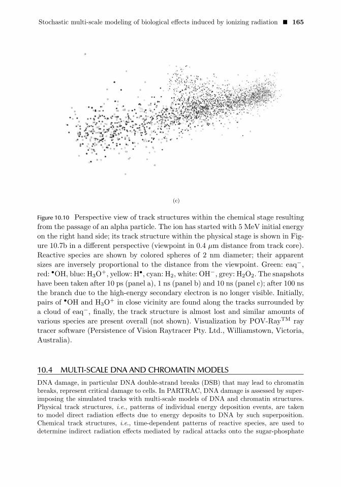
Stochastic multi-scale modeling of biological effects induced by ionizing radiation � 165
(c)
Figure 10.10 Perspective view of track structures within the chemical stage resulting
from the passage of an alpha particle. The ion has started with 5 MeV initial energy
on the right hand side; its track structure within the physical stage is shown in Fig-
ure 10.7b in a different perspective (viewpoint in 0.4 μm distance from track core).
Reactive species are shown by colored spheres of 2 nm diameter; their apparent
sizes are inversely proportional to the distance from the viewpoint. Green: eaq−,red: •OH, blue: H3O
+, yellow: H•, cyan: H2, white: OH−, grey: H2O2. The snapshots
have been taken after 10 ps (panel a), 1 ns (panel b) and 10 ns (panel c); after 100 ns
the branch due to the high-energy secondary electron is no longer visible. Initially,
pairs of •OH and H3O+ in close vicinity are found along the tracks surrounded by
a cloud of eaq−, finally, the track structure is almost lost and similar amounts of
various species are present overall (not shown). Visualization by POV-RayTM ray
tracer software (Persistence of Vision Raytracer Pty. Ltd., Williamstown, Victoria,
Australia).
10.4 MULTI-SCALE DNA AND CHROMATIN MODELSDNA damage, in particular DNA double-strand breaks (DSB) that may lead to chromatinbreaks, represent critical damage to cells. In PARTRAC, DNA damage is assessed by super-imposing the simulated tracks with multi-scale models of DNA and chromatin structures.Physical track structures, i.e., patterns of individual energy deposition events, are takento model direct radiation effects due to energy deposits to DNA by such superposition.Chemical track structures, i.e., time-dependent patterns of reactive species, are used todetermine indirect radiation effects mediated by radical attacks onto the sugar-phosphate

166 � A Guide to Outcome Modeling in Radiotherapy and Oncology
backbone or bases of the DNA macromolecule. Locations of DNA bases and sugar moietiesare considered as non-diffusing reaction partners of •OH and eaq− with certain reactionrate constants, in competition with all other species. Reactions of •OH with sugar leadwith high probability to DNA strand breaks from indirect effects, reactions with bases toindirect base damage. Otherwise, the merged atoms of the chromatin model define a volumenot filled with liquid water and thus not accessible to reactive species; those entering it areassumed to be scavenged and removed from further water radiolysis simulation.
Figure 10.11 DNA double-helix model with double-strand break. Spheres repre-
sent individual atoms of phosphate group (blue), deoxyribose (white, gray), ade-
nine (yellow), cytosine (pink), guanine (red) and thymine (green). Visualisation
by POV-RayTM ray tracer software (Persistence of Vision Raytracer Pty. Ltd.,
Williamstown, Victoria, Australia).
The target structures of DNA and chromatin in PARTRAC start with an atomic modelrepresentation of the DNA double-helix (Figure 10.11) and of a histone molecule based onX-ray crystallography data [433]. A DNA segment wrapped around a histone octamer servesas a model of the nucleosome, the most elementary repeating motif in chromatin. The nextlevel of chromatin organization, the 30 nm fiber, is obtained by positioning one nucleosomeafter the other into a corresponding virtual tube and by connecting them with a linkerDNA helix. The arrangement of subsequent nucleosomes determines the overall chromatinfiber structure. This is still a debated issue: Chromatin structures seem not to be uniform

Stochastic multi-scale modeling of biological effects induced by ionizing radiation � 167
and regular, but have to be viewed in the context of specific biological functions [434].The two-start zigzag topology and the type of linker DNA bending that defines solenoidmodels may be simultaneously present in a chromatin fiber with a uniform 30 nm diameter[435]. The DNA model in PARTRAC has the capability to describe regular or stochasticarrangements of nucleosomes in solenoidal as well as zigzag or crossed-linker topology [436].In order to cope with the amount of DNA of about 6 Gbp (6× 10⁹ base pairs) in a humandiploid cell, short pieces of a 30-nm chromatin fiber are used as building blocks for the entiregenome. Five types of basic fiber elements are defined within cubic voxels of 40 or 50 nmedge length in which the chromatin fibre connects the bottom plane with one of the otherfive walls of the cube. For a seamless connection of these building blocks, the interface struc-ture has to be identical. The interface may be reduced to a single nucleosome positionedbetween two boxes (see Figure 10.12); this allows consideration of two basic sets of buildingblocks with different compaction so as to describe hetero- and euchromatic structures [271].When several nucleosomes are cut at the interface [290], the chromatin fiber may becomevery compact, with the underlying building block structure hardly discernible. The buildingblocks are generated by a special trial-and-error algorithm using the Monte Carlo technique:under given boundary conditions of fiber structure parameters and the already positionednucleosomes, an additional nucleosome is placed, the linker DNA determined, and all thenewly positioned atoms are tested for spatial overlap with the formerly arranged ones. Inorder to setup the building blocks for a highly compact chromatin fiber (with about 6 nu-cleosomes per 10 nm fiber length), the above trial-and-error procedure has to be executedseveral million times.
With a given set of building blocks for the fiber structure, the next higher-order chro-matin structure is provided by a path of linked voxel elements on a regular three-dimensionalgrid with side length corresponding to the building blocks, combined with an algorithm fortracing their orientation. This path is established based on data provided by a 1-Mbp spher-ical chromatin domain model [290]. The chromatin domain centers are taken as anchor sitesof chromatin loops and in the DSB repair model as fixed nuclear attachment sites: thechromatin path periodically departs from the center and approaches it again until about 1Mbp is allocated by the formed loops; the path is then directed to the next chromatin do-main. The length and territorial organization of the chromosomes within the G0/G1 phaseis provided by the number and locations of the chromatin centers. Figure 10.13 shows thechromatin fiber path model of the chromosomes in an elliptical fibroblast nucleus.

168 � A Guide to Outcome Modeling in Radiotherapy and Oncology
Figure 10.12 Chromatin fibre model. Five basic fiber elements are seamlessly con-
nected. The elements are cubic boxes with 40 nm side length. A linear element on
the left hand side is in sequence with the four types of bent elements. The single
nucleosome in the interface layer allows linkage with other sets of elementary boxes,
either compact ones representing heterochromatin (shown) or loose ones with lower
numbers of nucleosomes that correspond to euchromatin (not shown). Spheres rep-
resent individual atoms of phosphate group (blue), deoxyribose (white), adenine
(yellow), cytosine (pink), guanine (red), thymine (green) and histone (turquoise).
Visualization by POV-RayTM ray tracer software (Persistence of Vision Raytracer
Pty. Ltd., Williamstown, Victoria, Australia).

Stochastic multi-scale modeling of biological effects induced by ionizing radiation � 169
Figure 10.13 Model of human fibroblast nucleus. Basic chromatin fibre elements
are represented by small straight or bent cylinders, forming tangled-up rope-like
structures; individual chromosomes are distinguished by their colours. Visualisa-
tion by POV-RayTM ray tracer software (Persistence of Vision Raytracer Pty. Ltd.,
Williamstown, Victoria, Australia).
10.5 INDUCTION OF DNA AND CHROMATIN DAMAGEDirect effects of ionizing radiation on DNA are in PARTRAC scored from energy deposits tothis macromolecule. Following experimental information on the sensitivity of DNA to irra-diation with low-LET radiation, a strand break is scored with a probability that depends onthe energy deposited to the sugar-phosphate backbone of DNA: energy deposits below 5 eVare ignored, all deposits above 37.5 eV are converted to strand breaks, and between these

170 � A Guide to Outcome Modeling in Radiotherapy and Oncology
two points a linear increase of breakage probability with the deposited energy is assumed.Indirect effects are scored from attacks of •OH radicals onto DNA. 65% of such interactionsonto a sugar are recorded as strand breaks. This probability results in a fraction of about13% of •OH interactions with DNA that leads to strand breaks, since attacks to bases areabout 4 times more frequent than those to the sugars. DNA double-strand breaks (DSB)are scored whenever breaks on opposite strands of the DNA molecule occur within 10 bpgenomic distance. Obviously, a DSB can be induced by two direct breaks, two indirect ones,or a combination of both. In addition, 1% probability is assumed for a conversion of single-strand breaks (SSB) into DSB, to account for experimentally observed DSB induction byvery low-energy (10 eV) photons and electrons and other findings supporting DSB induc-tion by single events [413]. In addition to strand breaks, also damage to DNA bases can beinvestigated with PARTRAC; in particular base lesions in a close vicinity to a DSB havebeen taken into account in the DSB repair simulation.
The results of PARTRAC simulations on DNA damage induction have been thoroughlybenchmarked against experimental data. Regarding the chemical stage, PARTRAC sim-ulations for SSB induced in linear DNA under varied lifetimes of hydroxyl radicals havebeen found in accord with measured data for different concentrations of dimethyl sulfoxide(DMSO), an efficient scavenger of these radicals; similarly good agreement with the data hasbeen obtained for SSB and DSB induced in SV40 minichromosomes [437]. As illustratedin Figure 10.14, experimentally observed yields for DSB induction after irradiation withlight ions of diverse energies (and thus diverse values of linear energy transfer, LET, whichis a measure of ionization density and, hence, of radiation quality) are well reproduced byPARTRAC simulations. The agreement of simulations with the data is even better whenplotted in terms of relative biological effectiveness (RBE) , since the simulations regularlysomewhat overestimate the measurements. The reported simulations take into account theexperimental limitations in detecting short DNA fragments. Actually, the simulations pre-dict that DNA fragment distributions after high-LET radiation are heavily skewed towardsshort fragments [438] that could not have been detected by the experimental protocol.Figure 10.15 shows that the simulations are also in good agreement with measured DSBdistributions [439] on genomic scales of about 20 kbp – 5 Mbp. On short genomic scales,PARTRAC simulations have reproduced the observed 78 bp and 190 – 450 bp peaks infragment size distributions [440], related to the nucleosome and short-scale arrangement inchromatin fiber [413]. Taken together, these benchmarks indicate that both track and chro-matin structures are represented properly in PARTRAC, since DNA fragmentation patternsnaturally reflect both of these structures.
In the following, simulation results are presented on initial DNA damage induced by avariety of light ions at energies from 250 down to 0.25 MeV/u [412]. Detailed information onthe simulation setup, methods and further results can be found in that reference. The yieldsare presented in dependence on the LET of the particles; the LET increases during particleslowing down up to a maximum value occurring around or below 0.5 MeV/u, after whichthe ion comes to rest within less than 10 μm. In Figure 10.16, the calculated induction ofDNA strand breaks due to direct and indirect effects is shown in dependence on the LETof the ion irradiation. The yield from direct effects is almost constant over a wide rangeof LET values. The yields from indirect effects, about 60% higher than those from directeffects at low LET values, decrease with increasing LET to values below the contributionsfrom direct effects. At higher energies, i.e., lower LET values the yields of strand breaks donot depend on ion type, but at low energies, i.e., approaching the maximum LET values

Stochastic multi-scale modeling of biological effects induced by ionizing radiation � 171
1 10 100 1000LET (keV/μm)
0
2
4
6
8
10
12yie
ld (
Gb
p-1
Gy
-1)
He
B
N
Ne
photons
exp. calc.
Figure 10.14 LET-dependent yield of DSB after photon and ion irradiation. Symbols:
experimental results from pulsed-field gel experiments [441, 442], lines: PARTRAC
simulations that disregard DSB linked to fragments shorter than 5 kbp. Adapted
from [412].
for a given ion, both direct and indirect effects tend to be lower than for heavier ions at thesame LET. High-LET radiation tends to induce multiple DSB in the close vicinity. SuchDSB cluster, equivalent to DSB++ in the notation by Nikjoo and coworkers [295, 13], arelikely processed by the cell as a single complex lesion. Thus such clustered DSB have beenmerged into a broken site (DSB site) counted only once in the analysis of PARTRAC dam-age simulation; also a separated DSB is counted as one DSB site. The LET-dependent yieldof DSB sites in Figure 10.17 is largely independent of particle type, and shows a pronouncedmaximum around about 200 keV/μm LET. Similar patterns have been reported in studieson cell survival upon exposure to radiations with diverse qualities [443]. The downwardtrend in simulation results for LET > 200 keV/μm follows from scoring multiple clusteredDSB as a single DSB site only; this is similar to disregarding fragments < 5 kbp in Fig-ure 10.14. The mentioned qualitative agreement with cell survival data indicates that thecells likely process DSB clusters together, rather than repairing individual DSB in a clusterindependently. The simulations allow one to look at the DSB clusters in more detail: TheLET-dependent formation of DSB clusters shown in Figure 18 culminates in a maximumaround 500 keV/μm LET for heavier ions or at the maximum LET value for lighter ions;however, the maximum yields decrease with increasing mass (or charge) of the ion. The
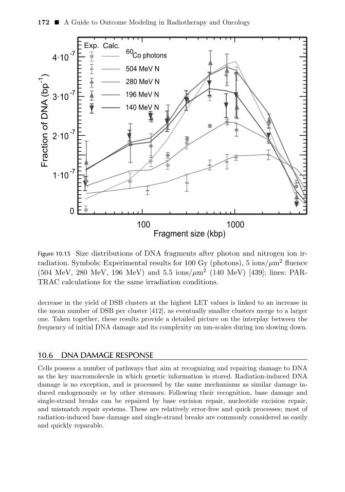
172 � A Guide to Outcome Modeling in Radiotherapy and Oncology
100 1000Fragment size (kbp)
0
1·10-7
2·10-7
3·10-7
4·10-7
Fra
ction o
f D
NA
(bp
-1)
Co photons
504 MeV N
280 MeV N
196 MeV N
140 MeV N
Exp. Calc.60
Figure 10.15 Size distributions of DNA fragments after photon and nitrogen ion ir-
radiation. Symbols: Experimental results for 100 Gy (photons), 5 ions/μm2 fluence
(504 MeV, 280 MeV, 196 MeV) and 5.5 ions/μm2 (140 MeV) [439]; lines: PAR-
TRAC calculations for the same irradiation conditions.
decrease in the yield of DSB clusters at the highest LET values is linked to an increase inthe mean number of DSB per cluster [412], as eventually smaller clusters merge to a largerone. Taken together, these results provide a detailed picture on the interplay between thefrequency of initial DNA damage and its complexity on nm-scales during ion slowing down.
10.6 DNA DAMAGE RESPONSECells possess a number of pathways that aim at recognizing and repairing damage to DNAas the key macromolecule in which genetic information is stored. Radiation-induced DNAdamage is no exception, and is processed by the same mechanisms as similar damage in-duced endogenously or by other stressors. Following their recognition, base damage andsingle-strand breaks can be repaired by base excision repair, nucleotide excision repair,and mismatch repair systems. These are relatively error-free and quick processes; most ofradiation-induced base damage and single-strand breaks are commonly considered as easilyand quickly reparable.

Stochastic multi-scale modeling of biological effects induced by ionizing radiation � 173
1 10 100 1000LET (keV/μm)
0
20
40
60
80
100
120yie
ld (
Gb
p-1
Gy
-1)
HHeLiBeBCNONe
indirect direct
Figure 10.16 Calculated LET-dependent yield of DNA strand breaks after ion irradi-
ation. Symbols connected by solid lines: contribution from indirect effects, dotted
lines: contribution from direct effects.
Double-strand breaks, on the other hand, represent a severe class of DNA damage sincenot only one but both DNA strands are affected; thus, some genetic information as wellas the connection of the broken ends may be lost. However, even DSB are repaired quiteefficiently; human cells typically repair more than 90% of radiation-induced DSB withina day post irradiation. Non-homologous end-joining (NHEJ) is the dominant DSB repairpathway in eukaryotic cells in the G1/G0 cell cycle phase; it aims at restoring the DNAintegrity in the absence of information on the original sequence, and as such is prone toerrors. Following DNA replication in the S phase, in the G2 phase the sister chromatid canbe used as a template for restoring the original sequence in an error-free way by the homol-ogous recombination pathway. Conceptually in between these two pathways is a third one,microhomology-mediated end-joining, which is based on using 5 – 25 bp microhomologoussequences downstream or upstream of the break to align the broken strands and try torestore the original sequence; this pathway operates in the S-phase, and is not free of errors.
The PARTRAC tools include a dedicated module to simulate DNA damage response.The framework of the model has been used so far to model DSB repair via NHEJ, since DSBare the most relevant lesions and the underlying initial DNA damage refers to the G0/G1phase of the cell cycle where NHEJ is the dominant rejoining process. The processing ofboth induced broken DNA ends as well as their motion is traced individually, so that not

174 � A Guide to Outcome Modeling in Radiotherapy and Oncology
1 10 100 1000LET (keV/μm)
0
5
10
15
20yie
ld (
Gb
p-1
Gy
-1)
HHeLiBeBCNONe
Figure 10.17 Simulated LET-dependent yield of DSB sites after ion irradiation. Iso-
lated DSBs as well as multiple DSBs in clusters are counted as one DSB site.
Adapted from [412].
only correct rejoining but also misrejoining and even the formation of chromosome aberra-tions can be assessed.
The following key steps of the NHEJ pathway [444] for the repair of DSB are modeledin PARTRAC (Figure 10.19): After a quick damage recognition and chromatin remodelingstep, DNA-dependent protein kinase (DNA-PK) has to attach to the induced DNA end.DNA-PK consists of two subunits, Ku70/80 and the catalytic subunit DNA-PKcs, whose at-tachments are actually modeled as two subsequent steps. Two DNA ends in close proximity,both with attached complete DNA-PK, form then a synaptic complex. Following the clean-ing steps in which nearby base lesions and/or additional single-strand breaks are removed,the final ligation takes place. The enzymatic processing is represented in the simulationas transferring the DNA end from one to another state, e.g., from a state with attachedKu70/80 to a state with complete DNA-PK. These transitions are described as processesin first order kinetics; for each process, the transition rate is a single parameter that entersthe model. For the early phase the transition rates between individual states have beenestimated from corresponding experimental data for Ku80 and DNA-PK attachment andturnover [445, 446]. The actual states and transitions of individual ends are simulated byMonte Carlo modeling analogous to the chemistry module; diffusive transport of DNA ends

Stochastic multi-scale modeling of biological effects induced by ionizing radiation � 175
1 10 100 1000LET (keV/μm)
0.0
0.5
1.0
1.5
2.0
2.5
3.0yie
ld (
Gb
p-1
Gy
-1)
HHeLiBeBCNONe
Figure 10.18 Simulated LET-dependent yield of DSB clusters (DSB++) after ion
irradiation. DSB clusters includes two ore more DSB within not more than 25 bp
distance. Adapted from [412].
alternates with potential changes of end states. The adopted time steps in typical calcula-tions are of the order of 0.1 s. The delayed repair of dirty DNA ends due to cleaning stepsin the model structure in Figure 10.19, combined with increasing fractions of dirty endswith increasing LET of the irradiation, leads to repair kinetics depending on the radiationquality that corresponds to measured data after irradiation with photons or nitrogen ionsof different LET, as shown in Figure 10.20.
In parallel to the enzymatic processing, the mobility of the DNA ends during repairis accounted for by a stochastic model of DNA end mobility, conceptually similar to theone used for reactive species in the chemical track structure module. However, the diffusivemotion of the DNA ends is confined by chromatin fibres being assumed to be attached atnuclear attachment sites and, for short fragments, by a maximum distance to the other endof the fragment corresponding to the genomic length of the fragment. The fibre compact-ification is gradually released, i.e. the radius of the sphere in which the end may diffusearound the nuclear attachment site is increased with time. With these mechanisms the ob-served sub-diffusive mobility of telomeres and induced DNA ends [447] is reproduced by thecalculations [448, 271].

176 � A Guide to Outcome Modeling in Radiotherapy and Oncology
clean
DNA end
dirty
DNA end
DNA end
mobili ationz
and chromatin
rearrangement
attachment of
Ku70/Ku80
attachment of
DNA-PKcssynapsis
final
ligation
end processing
cleaning
of nearby
lesions
Figure 10.19 Simplified scheme of DSB repair model in PARTRAC.

Stochastic multi-scale modeling of biological effects induced by ionizing radiation � 177
0.1 1 10Repairtime[h]
0.0
0.2
0.4
0.6
0.8
1.0F
ractio
no
fre
sid
ua
lDS
BExp. Calc.
225 keV/μm N ions
175 keV/μm N ions
80 keV/μm N ions
Co -rays60
γ
Figure 10.20 Kinetics of DSB repair after photon and nitrogen ion irradiation. Sym-
bols: experimental data [449], lines: PARTRAC calculations.
Throughout this procedure, individual DNA ends induced by the DSBs are followedindependently and in a stochastic manner. Hence it may happen that one end has alreadyattached a molecule of DNA-PK but its original partner not yet (or has diffused away). Ifanother DNA end with attached DNA-PK is found in close proximity, the two ends forma synaptic complex and, if the complex does not break, finally get ligated. Through thisinterplay of enzymatic processing and spatial mobility, not only correct rejoining but alsomisrejoining is simulated. If the two ligated segments used to belong to different chromo-somes, a chromosomal aberration is scored. Upon having complemented the simulationswith information on the location of centromeres, PARTRAC has been used formodeling theinduction of dicentric chromosomes, i.e., misrejoined chromosomes that contain fragmentswith centromeres from two different chromosomes. Without adjustment of model parame-ters, the simulations have correctly reproduced the dose dependence, although the absoluteyields of dicentrics for gamma and alpha-particle irradiation were overestimated [271].
The repair module in PARTRAC provides a powerful framework that can be extendedin many respects. One example is simulating the action of individual molecules of repairenzymes that mediate certain steps in the repair process instead of adopting first orderkinetics with a given rate constant [450]. The drawback of such a detailed approach is theincrease in the number of parameters to describe enzyme production, mobility, reactionradius, time constant for repopulation, nonlinear features such as feedback or upregulationetc., which are largely not known and can hardly be derived from their impact on the cal-

178 � A Guide to Outcome Modeling in Radiotherapy and Oncology
culated kinetic and outcome of the repair process. Another example are changes in DSBend states that are allowed only under certain boundary conditions, such as its overhanglength, which may also restrict the formation of a synaptic complex between DSB ends.Consideration of a maximum spatial distance of the ends of short DNA fragments forcesthe DNA ends to stay in proximity during diffusion; however, without further restrictionthis leads to high numbers of small rings: about 75% of the rings are smaller than about10 kbp [271]. To account for the stiffness of the DNA helix that is seen in the linear shortfragment structures due to DSB in plasmid DNA, the formation of rings can be suppressedbelow a certain genomic size, usually a few kbp.
The main aim of the model is to test hypotheses on key mechanisms during DNA dam-age response, such as the origin of misrejoining of broken DNA ends, the reason for slowlyrepairing DSB or the cause for unrejoined DSB ends after long repair times. For a solidtest it is not sufficient to yield an agreement under prevailing hypotheses but to show alsothe failure of alternative hypotheses. However, the calculated modeling endpoints may notdepend in a pronounced way on the tested mechanisms. Such result has been obtained fordifferent hypotheses on the origin of misrejoining where only DNA end mobility turned outto be trivially indispensable [296]. It is generally accepted that the complexity of initialDNA damage has a high impact on biological effects of radiation. However, the relativebiological effectiveness for reproductive cell death culminates around LET values of 100– 200 keV/μm [443], whereas the formation of DSB clusters and their complexity is stillrising with LET. This highlights the need for a more detailed evaluation of DNA damagedistribution on different scales.
In this situation innovative microbeam experiments have provided unprecedented datafor DNA damage response model testing and development. These experiments offer a sep-aration of the nanometre-scale clustering of radiation-induced damage from its clusteringon micrometre scales, which are otherwise closely interrelated in conventional experimentswith different radiation qualities [451]. Specifically, high-LET irradiation by carbon ions of55 MeV (LET: 310 keV/μm) delivered on a quadratic matrix with 5.4 μm side length hasbeen mimicked by bunches of 117 protons of 20 MeV (LET: 2.6 keV/μm) or 5 lithium ionsof 45 MeV (LET: 60 keV/μm) focused to spots of sub-μm size and delivered on the samematrix; secondly, the matrix size has been varied with related change of ions per spot tomaintain a constant dose to the cells. The induction of dicentrics has been determined asthe biological endpoint: an increase with the LET of the ions but also a pronounced effectof focusing for protons and lithium ions has been found; both were initially not adequatelyreproduced by PARTRAC model calculations [452]. After extensive parameter studies, rel-atively good agreement between experiment and model calculations has been obtained, seeFigure 10.21, regarding the focusing effect (except the largest matrix size) and the LETeffect of the incident ions. In this simulation, misrejoining events result primarily from asmall fraction of DSB ends which lose their proximity to the corresponding DSB end dueto high mobility in the early phase of DSB repair. Including other possible mechanismsleading to misrejoining, such as more frequent break-up of synaptic complexes or exchangeof DNA ends upon interaction of two such complexes, has reduced the conformity with thedata; yet alternative hypotheses continue to be tested aimed at finding a scenario with animproved agreement with the measured data and expectations on endpoints such as un-rejoined breaks after one day repair time . In spite of these limitations, the induction ofchromosomal exchange aberrations has turned out to correlate closely with the probability

Stochastic multi-scale modeling of biological effects induced by ionizing radiation � 179
of clonogenic cell death.
0 2 4 6 8 10 12
Irradiation matrix size ( )μm
0.0
0.1
0.2
0.3
Dic
en
tric
sp
er
ce
ll
exp. calc.
20 MeV H
45 MeV Li
55 MeV C
Figure 10.21 Induction of dicentrics after spot matrix irradiation by ion microbeam.
Alternative numbers of ions have been focused to sub-μm spots (1, 117, 234 and
468 for H, 1, 5, 10 and 20 for Li, 1 for C) and spots applied on a regular matrix
pattern, all corresponding to a unique dose of about 1.7 Gy. Circles: Dicentric
chromosomes scored in hybrid human-hamster AL cells [452]. Crosses and lines:
PARTRAC simulations.
10.7 MODELING BEYOND SINGLE-CELL LEVELAs is generally the case in modeling complex multi-scale systems, when moving towards alarger scale, only simplified characteristics of the processes underpinning a smaller scale canbe represented. Models on tissue and organ level thus hardly can account for full details oftrack structures, DNA damage and its repair included in PARTRAC as described above.Yet, PARTRAC has been successfully used in pilot studies on intercellular communication.Radiobiological experiments on so-called bystander effects have demonstrated that unir-radiated cells exposed to medium transferred from irradiated cells show similar responsesas if they were irradiated directly, including DNA damage induction or cell killing [453].PARTRAC simulations have been used to study alternative signal emission scenarios con-sistent with an observed threshold-like behaviour of bystander effects, which show an onsetat doses around 2 mGy of gamma irradiation [454]. Signal emission scenarios assumingabove-threshold energy deposits to mitochondria and signal amplification by neighbor cellshave been found consistent with the data [455]. Independent of PARTRAC simulations,non-linear response of bystander cells to the signals has been modelled [455, 456].

180 � A Guide to Outcome Modeling in Radiotherapy and Oncology
Another experimental system of intercellular communication whose radiation-inducedmodifications have been studied in detail is the selective removal of precancerous cells byapoptosis upon signaling by their normal neighbors. This intercellular induction of apop-tosis likely represents a natural anti-carcinogenic mechanism [457]; mechanistic modelingsuggests that this process is capable of stopping the growth of a population of precancer-ous cells, leading to a kind of dormancy [458]. Cell-culture experiments have shown thationizing radiation may enhance the underlying signalling and the resulting removal of pre-cancerous cells by apoptosis [459]. However, for in vivo conditions of early carcinogenesis,where a small population of precancerous cells is challenged by a large, dense populationof normal cells and the signaling species possess shorter lifetimes, the modeling predictsthat this anti-carcinogenic process be reduced upon radiation exposure [460]. This model-ing prediction would thus remove the discrepancy between the well-known epidemiologicalevidence that ionizing radiation induces cancer and the mentioned radiobiological exper-iments. To facilitate the urgently needed experimental benchmarking of this prediction,conditions have been formulated under which such inversed behavior is predicted alreadyand which, contrary to in vivo conditions, are achievable in cell-culture experiments; themodeling predictions thus await experimental verification.
10.8 CONCLUSIONSPARTRAC represents a state-of-the-art tool for stochastic multi-scale modeling of the bio-logical effects of ionizing radiation on subcellular and cellular scales. It integrates knowledgeon radiation physics, chemistry and biology. It provides means to test alternative hypotheseson the processes and mechanisms that underpin the observed biological effects. It also helpsinterpret the data and interpolate between or even extrapolate outside measured regimens,even to conditions and/or to the level of detail hardly accessible experimentally.
Future activities in PARTRAC development shall include linking it with a macroscopicradiation transport code to facilitate its applications in medical physics and to enable ad-dressing biological effects over spatial scales up to decimetres relevant in therapeutic appli-cations of radiation. It is also planned to propose a module to simulate cell killing basedon track structure calculations for initial DNA damage and subsequent modeling of DNAdamage response. On the one hand, such a detailed mechanistic model would serve as abenchmark to existing, rather descriptive models; on the other hand, it would extend PAR-TRAC applicability to an endpoint of utmost relevance to medical physics and radiationtherapy. It is also desirable to address the biological variability between different cell types,in particular regarding their capability to repair radiation-induced DNA damage. Likewise,one shall continue extending the scope of mechanistic modeling beyond the single-cell level.Last but not least, efforts shall be made to reduce the computational expensiveness, enhancethe predictive power and enable a widespread use of PARTRAC.

C H A P T E R 11
Multi-scale modelingapproaches: application inchemo– andimmuno–therapiesIssam El Naqa
CONTENTS
11.1 Introduction . . . . . . . . . . . . . . . . . . . . . . . . . . . . . . . . . . . . . . . . . . . . . . . . . . . . . . . . . . . . . 18211.2 Medical oncology treatments . . . . . . . . . . . . . . . . . . . . . . . . . . . . . . . . . . . . . . . . . . . 183
11.2.1 From chemotherapy to molecular targeted agents . . . . . . . . . . . . . . 18311.2.2 Immunotherapy . . . . . . . . . . . . . . . . . . . . . . . . . . . . . . . . . . . . . . . . . . . . . . . . . 184
11.3 Modeling types . . . . . . . . . . . . . . . . . . . . . . . . . . . . . . . . . . . . . . . . . . . . . . . . . . . . . . . . . . 18511.3.1 Continuum tumor modeling . . . . . . . . . . . . . . . . . . . . . . . . . . . . . . . . . . . . 18511.3.2 Discrete tumor modeling . . . . . . . . . . . . . . . . . . . . . . . . . . . . . . . . . . . . . . . . 18811.3.3 Hybrid tumor modeling . . . . . . . . . . . . . . . . . . . . . . . . . . . . . . . . . . . . . . . . . 189
11.4 Modeling examples . . . . . . . . . . . . . . . . . . . . . . . . . . . . . . . . . . . . . . . . . . . . . . . . . . . . . 19011.4.1 Modeling of chemotherapy . . . . . . . . . . . . . . . . . . . . . . . . . . . . . . . . . . . . . . 19011.4.2 Modeling of immunotherapy . . . . . . . . . . . . . . . . . . . . . . . . . . . . . . . . . . . . 192
11.5 Software tools for multi-scale modeling . . . . . . . . . . . . . . . . . . . . . . . . . . . . . . . . 19311.6 Conclusions . . . . . . . . . . . . . . . . . . . . . . . . . . . . . . . . . . . . . . . . . . . . . . . . . . . . . . . . . . . . . 194
ABSTRACTMulti-scale modeling of cancer growth and treatment response would allow better under-standing of the different biophysical and biochemical interactions at the molecular, cellular,tissue, and organ levels. Different mathematical models ranging from continuum, discrete,to hybrid have been proposed and evaluated in different theoretical and experimental set-tings. These process models not only can help explain the complex tumor-treatment systembut can also be used to personalize treatment single or combined modality regimens andpredict their efficacy. In this chapter, we will present examples of such modeling approachesand discuss its ability in the cases of chemotherapy drugs and immunotherapy agents.
181

182 � A Guide to Outcome Modeling in Radiotherapy and Oncology
Keywords: outcome models, multi-scale models, chemotherapy, immunotherapy.
11.1 INTRODUCTION
MULTI-SCALE modeling is a form of mathematical models that is routed in physicalsciences as a tool that allows solving complex problems at multiple temporal and
spatial scales. The complexity of cancer and its dynamical “carcinogenesis” processes andtheir interaction with their host immune system and therapeutic agents at varying scalesinvite the application of such advanced modeling schemes. These models can guide andoptimize response to therapy and would allow making quantitative predictions concerningtheir functional behavior and the physiochemical parameters that influence cancer response[461, 462]. Multi-scale models can complement mathematical tools already used in clinicaland cancer biology studies and enrich the library of treatment outcome prediction modelsby challenging current paradigms and shaping future research in cancer outcomes [463, 464].The multi-scale framework fro modeling cancer dynamics is presented in Figure 11.1 [464].
Cancer is a diverse family of diseases (about 100 known cancers) that is characterizedby an abnormal growth of cells that acquired the ability of uncontrolled progression andinvasion of surrounding tissues and disrupting their vital functions and leading to patientdeath. Biologically, cancer cells comprise of six major tumor hallmarks that underlie theirgenetic characteristics: sustained proliferative signaling, evasion of growth suppressors, re-sistance to cell death, replicated immortality, induction of angiogenesis, and activation ofinvasion and metastasis [465], which are the subject of active multi-scale modeling. Amongthese we will focus on the first four in our modeling description below. The dynamics ofmutation accumulation in cancer are typically modeled in computational biology by usinga fixed-size stochastic Moran process while metastasis dynamics are modeled by stochasticbranching process [462].
Patients diagnosed with cancer have multiple treatment options to choose from depend-ing on their disease type and its status. Typically, a patient with localized and early stagedisease would receive surgery, benefit from watchful waiting or active surveillance as inprostate cancer [466], or the use of medication for palliative purposes, rather than curativepurposes, as in certain types of leukemia [467]. However, patients at more advanced stagesof disease would receive chemoradiotherapy, molecular targeted therapy, immunotherapy, ora combination of these treatment modalities. In a previous chapter (Chapter 10), the focuswas primarily on on multi-scale modeling in radiation oncology using Monte Carlo (MC)techniques; therefore, here will present examples from chemo- and immuno-therapies. How-ever, the ideas could be directly generalized to other treatment modalities. Furthermore,it is currently an open question on how best to combine a specific immunotherapy agentwith chemotherapies, targeted therapies, surgery or radiation, in which both the timing,the concentration profile and the synergistic combinations need to be identified [463].

Multi-scale modeling approaches: application in chemo– and immuno–therapies � 183
Figure 11.1 Schematic illustration of the biological scales of significant relevance
for multi-scale cancer modeling including atomic, molecular, microscopic (tis-
sue/multicellular), and macroscopic (organ) scales. Different scales represent dif-
ferent spatial and temporal ranges; the methods for modeling these distinct scales
differ as well. Multi-scale cancer modeling requires the establishment of a linkage
between these scales.
11.2 MEDICAL ONCOLOGY TREATMENTS11.2.1 From chemotherapy to molecular targeted agentsThere are different categories of chemical agents that aim to eradicate tumor cancers [468].Among the most common ones are alkylating agents, which substitute an alkyl groups(hydrocarbon) for a hydrogen atom of an organic compound including DNA (e.g., Temo-zolomide). There are also antibiotics (e.g., Doxorubicin, Blemoycin). Other common agentsare antimetabolites (e.g., Methotrexate, 5-Fluorouracil,Taxanes,vinca alkaloids). Anotheragents that do not fall into any of these classes include platinum compounds (Cisplatin)and topoisomerases DNA winding enzymes inhibitors. Recently, more signaling pathwaymolecular targeted agents have been developed such as anti-epidermal growth factor recep-tor (EGFR) (e.g.,Cetuximab or Erbitux) [469]. In addition to the agent type and dosage,the timing of the administration of the agent can influence treatment response. Chemother-apy could be administrated after the completion of the local treatment such as radiationand is called adjuvant chemotherapy; if administered before the local treatment and iscalled induction chemotherapy, or, if given during local treatment, it is called concurrentchemotherapy. In particular, concurrent chemoradiation has been demonstrated to be ef-fective in the treatment of several cancers, in which the chemotherapy agent can act asa radiosensitizer by aiding the destruction of radiation resistant clones or act systemati-

184 � A Guide to Outcome Modeling in Radiotherapy and Oncology
cally and potentially eradicate distant metastases [470]. However, it is noted that despitetherapeutic advances in molecular targeted therapy (e.g., EGFR/ALK inhibitors in lungcancer), the vast majority of cancer patients do not benefit from such treatment and wouldstill receive generic cytotoxic agents [471]. A timeline of chemotherapy agents is shown inFigure 11.2 [468].
Figure 11.2 Timeline — The history of chemotherapy [468].
11.2.2 ImmunotherapyImmunotherapy by checkpoint blockade (CPB) has emerged as a promising therapeutic al-ternative for these tumors with a high degree of heterogeneity often caused by high somaticmutation burden (as in tobacco associated lung cancers). Immune tolerance is mediatedin part, by cytotoxic T-lymphocyte-associated antigen 4 (CTLA-4) or expression of pro-grammed death-ligand 1 (PD-L1) by the tumor and infiltrating immune cells. These check-points act as negative regulators of T-cell immune functions. The roles of CTLA-4 and PD-1in inhibiting immune responses, including antitumor responses, are largely distinct. CTLA-4is thought to regulate T-cell proliferation early in an immune response, primarily in lymphnodes, whereas PD-1 suppresses T cells later in an immune response, primarily in peripheraltissues as shown in Figure 11.3 [472]. In case of PD-1, for instance, PD-L1 binds to its cog-nate receptor, programmed death-1 (PD-1), on T cells and macrophages, profoundly alteringtheir proliferation and function [473]. Blocking PD-1 or PD-L1 promotes anti-tumor immu-nity by promoting a tumor-reactive adaptive and innate immune response [474]. Recently,published clinical trials of immune checkpoint inhibitors in metastatic lung cancer patientsinduced improved overall response rate of 15-20% with a median survival of 9-12 months, forinstance [475]. However, prognostic and predictive models are not clearly established, andan inability to precisely identify the patients who will benefit, limits CPB promise [476] andplaces patients at higher risk for immune related toxicities [477]. Therefore, more sensitiveand specific models that can explain and predict immunotherapy responsiveness would beparticularly useful.

Multi-scale modeling approaches: application in chemo– and immuno–therapies � 185
Figure 11.3 CTLA-4 and PD-1 pathway blockade. CTLA-4 blockade allows for acti-
vation and proliferation of more T-cell clones, and reduces Treg-mediated immuno-
suppression. PD-1 pathway blockade restores the activity of antitumor T cells that
have become quiescent. A dual pathway blockade could have a synergistic effect,
resulting in a larger and longer lasting antitumor immune response. CTLA-4 indi-
cates cytotoxic T-lymphocyte-associated antigen 4; MHC, major histocompatibility
complex; PD-1, programmed death 1; PD-L1, programmed death ligand 1; TCR,
T-cell receptor; Treg, regulatory T cell [472].
11.3 MODELING TYPESModels for cancer could be categories based on how the tumor tissue is represented intocontinuum models, discrete cell-based models, or a combination of both (hybrid) usingmulti-scale settings. There are several excellent textbooks and review articles dedicated tothis subject [478, 463, 462] that can provide the interested reader with more details beyondthe scope of this chapter.
11.3.1 Continuum tumor modelingContinuum tumor models are based on the reaction-diffusion differential equations, whichattempt to provide a description of the tumor cell density, the extracellular matrix (ECM),the matrix degrading enzymes (MDEs), and the concentrations of cell related substrates(e.g., glucose, oxygen, and growth factors and inhibitors) [478]. These methods employ anordinary differential equation (ODE) or partial differential equation (PDE) to representthe tumor and its microenvironment. The models could be single-species (e.g., single-phasetumors) or multiphase (mixture) models , which have been developed to describe detailedinteractions between multiple solid cell species and extra- or intracellular liquids [478]. These

186 � A Guide to Outcome Modeling in Radiotherapy and Oncology
models further try to model the two main types of tumor growth, namely; avascular (withno blood vessels) and vascular (with blood vessels [angiogenesis]). These models are typi-cally confined to a spherical geometry (spheroids) to simplify numerical calculations. Thebasic tumor growth (avascular) model would represent tumor cells proliferating in such away that they form a small sphere-like structure without direct access to the vasculature.During this avascular growth, the tumor cells receive oxygen, nutrients, and growth fac-tors via the diffusion process from the surrounding host tissue. Mixture models incorporatemore detailed biophysical processes than can be accounted for in single-phase models, andthey provide a more general framework for modeling solid tumor growth with avascularor vascular capabilities. Phenotypic and genetic heterogeneity (e.g., mutations) in the cellpopulation can be represented mathematically, and this is a critical improvement towardsmore realistically simulating mutation-driven heterogeneity [478, 462].
As a representative example of this category, we will briefly describe the model developedbyWise et al. [479]. The model follows from the laws of conservation of mass and momentum,and consists of a fourth-order nonlinear advection-reaction-diffusion equations (of the Cahn-Hilliard -type) that describe the growth of various tumor-cell species and diffusion reactionequations representing the time evolution of the environmental substrate concentrationsthat affect tumor growth. The evolution equation of the total tumor volume fraction model(φT ) is given by:
∂φT
∂t= M∇(φT∇μ) + ST −∇ · (uSφT ), μ = f(φT )− ε2∇2φT , (11.1)
where M > 0 is the mobility constant related to phase separation between tumoral andhealthy tissues; ST is the net source of tumor cells; uS is the tissue velocity f(φ) = φ2(1−φ)/4, which is a double-well potential; ε > 0 is the parameter specifying the thickness ofthe interface between healthy and tumoral tissues. A nonlinear multigrid scheme using anadaptive-mesh and finite difference methods is used to solve equation 11.1 efficiently forcomplex tumor morphologies [479]. A 3D simulation example is shown in Figure 11.4.

Multi-scale modeling approaches: application in chemo– and immuno–therapies � 187
Figure 11.4 A 3D simulation during the growth of an asymmetrical tumor at different
time points [479].

188 � A Guide to Outcome Modeling in Radiotherapy and Oncology
11.3.2 Discrete tumor modelingDiscrete modeling has enjoyed a long history in applied mathematics and biology since theseminal work of von Neumann in applied lattice crystals. These models are divided into twocategories: lattice-based (e.g., cellular automata) and lattice-free (e.g., agent-based). Bothapproaches track and update individual cells according to a set of biophysical rules. Typi-cally these models involve a composite discrete-continuum approach in the sense that themicroenvironmental variables (glucose, oxygen, extracellular matrix, growth factors, etc.)are described using continuum fields while the cells are discrete. In lattice-based modeling ,the cells are confined to a 2D or 3D lattice and each mesh point in the lattice is updated intime according to deterministic or stochastic rules derived from physical conservation lawsand biological constraints. Cellular automata (CA) is considered a special case, where amesh point represents an individual cell. In case of lattice-free (agent-based) models , theydo not restrict the cells’ positions and orientations in space. This allows more flexibilittyand accurate coupling between the cells and their microenvironment providing the individ-ual cells in the model with more freedom in terms of motility, death, or survival. This isespecially useful in modeling cases like angiogenesis, carcinogenesis, immune system attackson tumor cells, and metastasis [480]. However, this freedom may come at a hefty computa-tional cost when compared with continuum approaches, especially when dealing with largesystems with millions of cells.
As an example of these models, we will consider a lattice-based approach using an ex-tended Q-Potts model, which originated in statistical mechanics to study materials. Themost common approach utilizes the Q-Potts model to simulate cell sorting through differen-tial cell-cell adhesion and is known as the Graner-Glazier-Hogeweg (GGH) or cellular Pottsmodel (CPM) model [481] . In this approach, each cell is treated individually and occupiesa finite set of grid points within a Cartesian lattice; space is divided into distinct cellularand extracellular regions. Each cell is deformable with a finite volume. Cell-cell adhesionis modeled with an energy functional (Hamiltonian). A Monte Carlo algorithm is used toupdate each lattice point and hence change the effective shape and position of a cell. Al-though the description of the cell shape is less detailed than in the continuum (ODE/PDE)approaches described above, finite-size-cell effects are still incorporated.
Like any statistical mechanics system, the Hamiltonian is the main component to definein the GGH/CPM model and is determined by the configuration of the cell lattice. Theoriginal Hamiltonian proposed by Graner and Glazier included adhesion energies and area(volume) constraints for 2D (3D) tumors [481]:
H =∑
(i,j)neighborhood
J(τ(σi), τ(σj))(1− δ(τ(σi), τ(σj)) + λ∑i
(v(σi)− V (σi))2, (11.2)
where τ(σ) is the cell type associated with cell σ; J() is the surface energy determining theadhesion between two cells; δ is the Kronecker (tensor) product; v(σ) is the volume of cellσ, V (σ) is the target volume; and λ is a Lagrange multiplier determining the strength ofthe volume constraint. The Hamiltonian has been modified to control cell behaviors such aschemotaxis, elongation and haptotaxis by using other sub-lattices containing informationsuch as the concentrations of chemicals as shown in Figure 11.5 [482].

Multi-scale modeling approaches: application in chemo– and immuno–therapies � 189
Figure 11.5 Tumor invasion with homogeneous and heterogeneous ECM. (A) Inva-
sion front of tumor penetrating the stroma via viscous fingers. (B) Avascular tumor
model of Rubenstein and Kaufman, exploring invasion along ECM fibers. (C) Inva-
sion front of persistently moving cancer cells penetrate in fingers along ECM fibers
describe penetration dynamics even without cell division [482].
11.3.3 Hybrid tumor modelingThese models combine the advantages of continuum and discrete approaches in order tobetter simulate multi-scale multi-body complex tumors problems. They can provide morerealistic descriptions of microscopic mechanisms while efficiently evolving the entire systemto obtain macroscopic observations. These models typically contain one or more continuumand discrete components; each component is described by a set of equations that satisfy theconservation of mass and momentum. Using statistical mechanics, the connection betweenthe continuum and discrete mass and momentum could be established and the couplingmechanism could be derived, this could be further generalized across the different scalesand incorporate further available molecular and/or imaging information as depicted in Fig-ure 11.6 [478].
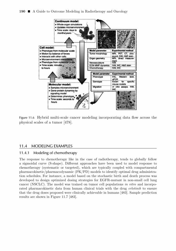
190 � A Guide to Outcome Modeling in Radiotherapy and Oncology
Figure 11.6 Hybrid multi-scale cancer modeling incorporating data flow across the
physical scales of a tumor [478].
11.4 MODELING EXAMPLES11.4.1 Modeling of chemotherapyThe response to chemotherapy like in the case of radiotherapy, tends to globally followa sigmoidal curve (S-shape). Different approaches have been used to model response tochemotherapy (systematic or targeted), which are typically coupled with compartmentalpharmacokinetic/pharmacodynamic (PK/PD) models to identify optimal drug administra-tion schedules. For instance, a model based on the stochastic birth and death process wasdeveloped to design optimized dosing strategies for EGFR-mutant in non-small cell lungcancer (NSCLC). The model was trained on tumor cell populations in vitro and incorpo-rated pharmacokinetic data from human clinical trials with the drug erlotinib to ensurethat the drug doses proposed were clinically achievable in humans [483]. Sample predictionresults are shown in Figure 11.7 [483].

Multi-scale modeling approaches: application in chemo– and immuno–therapies � 191
Figure 11.7 Targeted chemotherapy cancer modeling predictions to delay the devel-
opment of resistance. (A) PC-9 cell birth rate at erlotinib concentrations of 0, 1,
3, 10, and 20 μM . (B) PC-9 cell death rate as a function of increasing erlotinib
concentration. (C) PC-9/ER cell birth rate in the presence of erlotinib (0, 1, 3, 10,
and 20 μM). (D) PC-9/ER cell death rates as a function of increasing erlotinib
concentration. (E) Probability of preexisting T790M-harboring cells in a popula-
tion of 3 million cells initiating from one cell harboring just a drug-sensitive EGFR
mutation that grew in the absence of drug for a range of mutation rates (104 to 108
per cell division). (F) Expected number of resistant cells present in the population,
both averaged over all cases and averaged only over the subset of cases, where at
least one resistant cell is present. (G) An initial population of 750,000 cells, 10%
of which harbor T790M, treated with continuous low-dose erlotinib (1 and 3 μM)
selects for the emergence of T790M-harboring cells (green and black lines). The
addition of one or two high-dose erlotinib “pulses” (20 μM) followed by 1 μM for
the remaining days of a 7-day cycle decreases the expected number of resistant cells
(red and blue lines). (H) Analogous results as in panel (G) starting with an initial
population with 25% T790M-harboring cells.

192 � A Guide to Outcome Modeling in Radiotherapy and Oncology
In another study, the efficacy of a cytoxic chemotherapy drug (Doxorubicin) was simu-lated using a continuum approach with a vascular tumor model (cf. 11.3.1)[484]. The drugdistribution was represented by a diffusion-convection PDE. The toxicity of the drug tar-geted to the tumor cells is determined by the drug concentration and tumor cell activity,with higher concentrations of drug that are more likely to induce cell cycle transitions fromactive to quiescent or necrotic. The intravascular drug concentration can be predicted usingbody level PK/PD models as shown in Figure 11.8 [484].
Figure 11.8 Tumor morphology and chemotherapy drug (doxorubicin) distribu-
tion following three different drug administration concentrations (0.1, 1, and 10
mol/m3), [484].
11.4.2 Modeling of immunotherapyModulating the interplay between the immune system and cancer cells via immunotherapyalone or on in combination with other therapeutics is becoming one of the most promisingcancer treatment approaches. Due to the complexity of this interplay, computational mod-eling methods are playing a pivotal role [463]. A summary of such efforts using differentmodeling approaches is shown in Figure 11.9 [485]. For instance, an agent-based (cf. Section11.3.2) model was used to study the effects of a specific immunotherapy strategy againstB16-melanoma cell lines in mice and to predict the role of CD137 (tumor necrosis factor(TNF) receptor family) expression on tumor vessel endothelium for successful therapy [486].Another study applied a discrete-time pharmacodynamic model to illustrate the potentialsynergism between immune checkpoint inhibitors (PD1-PDL1 axis and/or the CTLA-4)and radiotherapy. The effects of irradiation were described by a modified version of thelinear-quadratic (LQ) model [487]. The model was able to explain the biphasic relationshipbetween the size of a tumor and its immunogenicity, as measured by the abscopal effect ,i.e., an induced non-localized immune response. Moreover, it explained why discontinuingimmunotherapy may result in either tumor recurrence or a durably sustained response in-dicating potential for better synergistic scheduling [487].
A continuum type model was developed to combine therapeutic effects from chemother-

Multi-scale modeling approaches: application in chemo– and immuno–therapies � 193
apy and immunotherapy was proposed by Pillis et al. by including the influence of severalimmune cell effector subpopulations (tumor antigen-activated CD8+ T cells, natural killer(NK) cells and total circulating lymphocytes), in addition to the concentrations of inter-leukin (IL)-2 and chemotherapy drug in the bloodstream [488]. However, such combinedmodeling approaches remains an active area of research today.
Figure 11.9 Summary of modeling efforts in immunotherapy [485].
11.5 SOFTWARE TOOLS FOR MULTI-SCALE MODELINGThere are several software tools for multi-scale modeling in the literature. Among the com-monly used ones is CompuCell3D. CompuCell3D is an open-source simulation environ-ment for multi-cell, single-cell-based modeling of tissues, organs and organisms. It uses theGlazier-Graner-Hogeweg (GGH) model as described above [489]. The software is written inC++ programming language and is constructed with a friendly object-oriented (modular)design. Models are described at a basic level using XML, but far greater versatility is af-forded by use of custom extensions written in the Python scripting language, through whichmuch of the model architecture can be accessed (a Simplified Wrapper and Interface Gener-ator (SWIG) interface exposes the C++ modules to Python). An example demonstration isshown in Figure 11.10. Other software tools that exist include EPISIM [490], Chaste [491],and PhysiCell [492].

194 � A Guide to Outcome Modeling in Radiotherapy and Oncology
Figure 11.10 COMPU3DCELL simulation software demonstration.
11.6 CONCLUSIONSMulti-scale modeling techniques (continuum, discrete, or hybrid) provide a useful and com-plementary role to other treatment outcome modeling schemes based on statistical or ma-chine learning techniques. Moreover, it allows for better mechanistic understanding of theinterplay between the tumor and various therapeutic agents. However, with increased com-plexity (parameterization in this case), further experimental and clinical data is required tomeet proper fitting requirements of these methods. This would demand closer collaborationsamong modelers, basic scientists and clinicians to achieve the potential of such a powerfulmathematical modeling approach to improve our understanding of cancer treatment out-comes, and address current open questions to how to prescribe a certain treatment regimenor optimize synergy of timing and dosing of multiple treatment modalities for localized ormetastatic cancers.

IVExample Applications in Oncology
195

C H A P T E R 12
Outcome modeling intreatment planningX. Sharon Qi
Mariana Guerrero
X. Allen Li
CONTENTS
12.1 Introduction . . . . . . . . . . . . . . . . . . . . . . . . . . . . . . . . . . . . . . . . . . . . . . . . . . . . . . . . . . . . . 19912.1.1 Review of the history and dose-volume based treatment
planning and its limitations . . . . . . . . . . . . . . . . . . . . . . . . . . . . . . . . . . . . . 19912.1.2 Emerging dose-response modeling in treatment planning and
advantages . . . . . . . . . . . . . . . . . . . . . . . . . . . . . . . . . . . . . . . . . . . . . . . . . . . . . . . 20012.2 Dose-response models . . . . . . . . . . . . . . . . . . . . . . . . . . . . . . . . . . . . . . . . . . . . . . . . . . . 202
12.2.1 Generalized equivalent uniform dose (gEUD) . . . . . . . . . . . . . . . . . . 20212.2.1.1 Serial and parallel organ models . . . . . . . . . . . . . . . . . . . 202
12.2.2 Linear-Quadratic (LQ) Model . . . . . . . . . . . . . . . . . . . . . . . . . . . . . . . . . . 20312.2.3 Biological effective dose (BED) . . . . . . . . . . . . . . . . . . . . . . . . . . . . . . . . . 20412.2.4 Tumor control probability (TCP) models . . . . . . . . . . . . . . . . . . . . . . 20412.2.5 Normal Tissue Complication Model (NTCP) models . . . . . . . . . . 206
12.2.5.1 Lyman-Kutcher-Burman (LKB) model . . . . . . . . . . . . 20612.2.5.2 Relative seriality (RS) model . . . . . . . . . . . . . . . . . . . . . . . 20712.2.5.3 Model parameters and Quantitative Analysis of
Normal Tissue Effects in the Clinic (QUANTEC) . 20712.2.6 Combined TCP/NTCP models –Uncomplicated tumor control
model (UTCP or P+) . . . . . . . . . . . . . . . . . . . . . . . . . . . . . . . . . . . . . . . . . . . 20812.3 Dose-response models for stereotactic body radiotherapy (SBRT) . . . . 208
12.3.1 Linear-Quadratic (LQ) model applied to SBRT . . . . . . . . . . . . . . . . 20812.3.2 Universal survival curve (USC) model . . . . . . . . . . . . . . . . . . . . . . . . . . 20912.3.3 Linear-Quadratic-Linear (LQL) model . . . . . . . . . . . . . . . . . . . . . . . . . 21012.3.4 Regrowth model . . . . . . . . . . . . . . . . . . . . . . . . . . . . . . . . . . . . . . . . . . . . . . . . . 21112.3.5 Dose limits for SBRT treatments . . . . . . . . . . . . . . . . . . . . . . . . . . . . . . . 211
12.4 Biological models in treatment planning . . . . . . . . . . . . . . . . . . . . . . . . . . . . . . . 21412.4.1 Plan evaluation . . . . . . . . . . . . . . . . . . . . . . . . . . . . . . . . . . . . . . . . . . . . . . . . . . 21412.4.2 Plan optimization . . . . . . . . . . . . . . . . . . . . . . . . . . . . . . . . . . . . . . . . . . . . . . . 215
197

198 � A Guide to Outcome Modeling in Radiotherapy and Oncology
12.4.3 Dose summation using biological models . . . . . . . . . . . . . . . . . . . . . . . 21512.4.4 Selection of outcome models and model parameters . . . . . . . . . . . 216
12.5 Commercially available treatment planning systems (TPS) employingoutcome models . . . . . . . . . . . . . . . . . . . . . . . . . . . . . . . . . . . . . . . . . . . . . . . . . . . . . . . . . 21612.5.1 Elekta Monaco system (Maryland Heights, MO) . . . . . . . . . . . . . . 21612.5.2 Philips Pinnacle system (Andover, MA) . . . . . . . . . . . . . . . . . . . . . . . . 218
12.5.2.1 Sensitivity of model parameters . . . . . . . . . . . . . . . . . . . . 21912.5.3 Varian Eclipse system (Palo Alto, CA) . . . . . . . . . . . . . . . . . . . . . . . . . 220
12.5.3.1 Objective functions in plan optimization . . . . . . . . . . . 22012.5.3.2 Plan evaluation . . . . . . . . . . . . . . . . . . . . . . . . . . . . . . . . . . . . . 22112.5.3.3 Sensitivity of model parameters . . . . . . . . . . . . . . . . . . . . 222
12.5.4 RaySearch RayStation (Stockholm, Sweden) . . . . . . . . . . . . . . . . . . . 22212.5.4.1 Plan evaluation tools . . . . . . . . . . . . . . . . . . . . . . . . . . . . . . . 22212.5.4.2 Plan optimization tools . . . . . . . . . . . . . . . . . . . . . . . . . . . . . 222
12.5.5 MIM (MIM Software Inc., Cleveland, OH) . . . . . . . . . . . . . . . . . . . . . 22212.5.5.1 Plan summation . . . . . . . . . . . . . . . . . . . . . . . . . . . . . . . . . . . . 22312.5.5.2 Plan evaluation . . . . . . . . . . . . . . . . . . . . . . . . . . . . . . . . . . . . . 223
12.6 Conclusions . . . . . . . . . . . . . . . . . . . . . . . . . . . . . . . . . . . . . . . . . . . . . . . . . . . . . . . . . . . . . 224
ABSTRACTThe goal of radiotherapy (RT) is to deliver the therapeutic radiation dose to the targetswhile minimizing potential complications to the adjacent normal structures. Physical quan-tities, such as dose and dose-volume metrics, have been used to optimize a treatment planand evaluate the quality of the plan. Such physical quantities are unlikely to predict patientbiological response, which is usually characterized by a nonlinear dose response relationship.Several dose-response models have been proposed and are expected to more closely reflectclinical goals and quantitatively predict treatment outcome. In recent years dose-responsemodels have been included in commercial treatment planning systems and play an increas-ingly important role in RT planning. In this chapter, we summarized the most commonlyused dose-response models and biological quantities, followed by the application of the mod-els in the treatment planning process, both for plan evaluation and/or plan optimization formajor commercial treatment planning platforms. The platforms are Monaco (Elekta, Mary-land Heights, MO, USA), Pinnacle (V8.0h, Philips Medical Systems, Andover, MA, USA),Eclipse (V10.0, Varian Medical Systems, Palo Alto, CA, USA), and RaySearch (RaySearchLaboratories AB, Stockholm, Sweden).
Keywords: radiotherapy treatment planning, dose-volume metrics, biological models, treat-ment outcome, treatment planning platforms.

Outcome modeling in treatment planning � 199
12.1 INTRODUCTIONThe ultimate goal of radiation treatment planning is to generate plans to deliver the ther-apeutic radiation dose to the targets while minimizing the complications to the adjacentnormal tissues. Historically, due to the lack of understanding of the underlying biologicalmechanisms and the sparsity of available clinical data, physical surrogates such as dose-volume endpoint have often been adopted to judge the quality of a radiation treatmentplan. However, such dose and dose-volume quantities are unlikely to predict patient specificbiological response, usually characterized by a nonlinear dose-response relationship. Bio-logical models, on the other hand, have been proposed for many decades and are expectedto more closely reflect clinical goals and quantitatively predict treatment outcome [493, 152].
Treatment planning tools that use biological models for plan optimization and/or eval-uation are available for clinical use. A variety of dose response models and quantities alongwith a series of organ-specific model parameters are included in these tools [152]. In fact,the major treatment planning platforms, such as Monaco (Elekta, Maryland Heights, MO,USA), Pinnacle (V8.0h, Philips Medical Systems, Andover, MA, USA), Eclipse (V10.0, Var-ian Medical Systems, Palo Alto, CA, USA), and RaySearch (RaySearch Laboratories AB,Stockholm, Sweden), have implemented a biological-based treatment planning module intoa routine treatment planning process for plan evaluation and/or plan optimization.
12.1.1 Review of the history and dose-volume based treatment planning and itslimitations
Current dose-volume based treatment planning is a result of the history of radiotherapy.In the 1960-70s, treatment planning was in its primitive stage prior to the application ofcomputers [493]. In the 1980s, 3-dimensional conformal radiotherapy (3D-CRT) technologybecame available allowing investigators to correlate the dose-volume information with clin-ical outcome data. This so-called ‘forward planning’ is no longer feasible for the emergingintensity modulated radition therapy (IMRT) as there are far too many degrees of freedomin IMRT planning.
Modern techniques such as IMRT often require some kind of optimization using powerfulcomputer software (so-called “inverse planning”). The user specifies the single or multipletreatment goals and lets the computer system find the best possible solutions. The treatmentgoals are often defined in terms of physical dose limits to different volumes, which arebased on clinical studies that demonstrate correlation between tumor control/complicationincidence and particular dose-volume metrics. For example, V20 (percentage of lung volumereceiving at least 20 Gy) is used to gauge the probability of a plan causing grade ≥ 2 or grade≥ 3 radiation pneumonitis [494]. However, there are a number of limitations associated withthe dose-volume based treatment planning approach as summarized below:
1. Dose-volume based treatment planning typically utilizes one or more organ-specificDVH constraints (e.g., V5, V10, V20, mean lung dose) that correlates with the com-plication based on previous experience. This correlation is typically specific to thetreatment delivery technique, i.e., IMRT or 3DCRT, beam arrangements, dose frac-tionation scheme, etc. Caution should be taken when the limits are clinically appliedbut were derived from other institutions, treatment techniques and/or planning sys-tems.

200 � A Guide to Outcome Modeling in Radiotherapy and Oncology
2. Optimization with dose-volume constraints requires substantial practice and experi-ence in selecting objectives and relative weights to meet planning goals. The trial-and-error method is generally adopted, which may be time consuming for some challengingcases and is highly dependent on the planner experience level.
3. Specifying multiple dose-volume constraints increases computational complexity of theinverse treatment-planning problem. Moreover, cost functions based on dose-volumeconstraints can lead to multiple local minima [495, 496], potentially leading to lessfavorable dose distributions [152].
4. Most current dose-volume based plan optimizations lack tools for routinely evaluatingbiologically based metrics alongside DVH metrics. Since dose distributions for plansdriven by biological methods constraints may differ substantially from those driven bydose-volume point constraints, evaluation tools are important as a basis for progressionto preferentially adopting biological methods in optimization.
12.1.2 Emerging dose-response modeling in treatment planning and advantagesDose-response based treatment planning, or biological-based treatment planning, however,is an emerging development that can further improve radiation plan quality when usedin conjunction with the dose-volume based treatment planning for plan evaluation andoptimization. The advantages of biological based treatment planning can be summarized asfollows:
1. Biological model based optimization is designed to reflect more realistic dose-responserelationships for the targets and OARs and quantitatively estimate TCP/NTCP prob-abilities in the selection of treatment plans. Instead of uniform dose distribution tothe target, a more inhomogeneous treatment plan may be expected compared to thecurrent dose-volume based optimization [497, 498].
2. Biological model based optimization may be more effective in OAR sparing. Whilemultiple dose-volume points are normally selected for dose-volume based inverse treat-ment planning optimization via trial-and-error method, a biological based objectivefunction, i.e., single EUD-based cost function with appropriate choice of a volumeeffect parameter, may lead to a better treatment plan in a more efficient way sincethe biological cost function controls greater space in the dose-volume domain.
3. Biological based plan evaluation provides additional biological metrics such as EUD,TCP, NTCP, UTCP, that are otherwise unavailable in dose-volume based plan eval-uation tools. Estimates of biological metrics are useful in the selection of rival plansthat may spare one OAR over the other or have crossing DVHs for a critical struc-ture. These situations are illustrated in Figure 12.1(a) and (b). Figure 12.1(a) showsa rectum DVH for two competing prostate plans. Both plans fulfill the clinical goalsbut the dose distributions are quite different so the knowledge of NTCP values couldbe useful in deciding between the competing plans. Figure 12.1(b) shows the DVHsfor esophagus and ipsilateral lung for two competing lung plans. One plan benefitsthe esophagus at the cost of more lung dose and vice versa with both plans havingsimilar target coverage and other OAR DVHs. Again, NTCP modeling could helpmake better clinical decisions in such cases.

Outcome modeling in treatment planning � 201
(a)
(b)
Figure 12.1 (a) Rectum DVH for two competing prostate plans. Both plans fulfill
the clinical goals but the dose distributions are quite different so the knowledge of
NTCP values could be useful in deciding among plans. (b) DVHs for esophagus and
ipsilateral lung for two competing lung plans.

202 � A Guide to Outcome Modeling in Radiotherapy and Oncology
12.2 DOSE-RESPONSE MODELS12.2.1 Generalized equivalent uniform dose (gEUD)The concept of generalized equivalent uniform dose (gEUD) assumes that any two dose dis-tributions are equivalent if they cause the same biological effect [499, 151]. More specifically,the gEUD is defined as the uniform dose that gives the same biological effect as a giveninhomogeneous dose distribution and can be calculated based on the power law dependenceof dose response for both tumor and organ-at-risk (OAR):
gEUD =
(∑i
νiDai
)1/a
(12.1)
where νi is the fractional organ volume within the target or OAR irradiation to dose Di.The parameter a is an organ-specific biological parameter. Figure 12.2 shows a set of DVHswith various degrees of inhomogeneity of the corresponding dose distributions that has thesame EUD.
The gEUD model is parameterized by the single biological parameter a, which is specificfor a pre-defined and quantifiable biological endpoint for given tumor and/or OAR. The pa-rameter a in gEUD and the Lyman model parameter n are inversely related as a = 1/n. AgEUD can be calculated directly from the dose calculation points or from the correspondingdose-volume histograms (DVHs). For a → ∞, gEUD approaches the minimum dose; thusnegative values of parameter a are generally used for tumors to penalize target cold spots.
Due to its simplicity, specifically the same gEUD formalism being applied to both targetsand OARs with a single parameter capturing different dosimetric characteristics of the bio-logical responses, the concept of gEUD is often utilized in plan evaluation and optimization.
12.2.1.1 Serial and parallel organ modelsFor normal organs, the concept of functional sub-units (FSU) is used to model the radia-tion response. FSUs may be arranged in serial, parallel, or a combination of both. Serialorgans involve FSUs in a line, meaning the organ fails if a single FSU is susceptible to highpoint doses and therefore the volume effect is small and the response depends mostly onthe maximum dose. Since gEUD approaches the maximum dose as a → ∞ a large value isoften used to characterize serial organs. The spinal cord and the gastrointestinal tract aretypical serial organs.
On the other hand, each FSU in a parallel organ is able to function independently ofthe others. Loss of a single FSU leads to a slight decrease in function of the organ. Parallelorgans are more sensitive to volume effects and complications are assumed to occur after asubstantial fraction of FSUs are damaged. A small value of the parameter a (close to 1) ingEUD is typically used for parallel organs, and therefore gEUD approaches the mean dose.Typical parallel organs include the liver and the kidneys.

Outcome modeling in treatment planning � 203
Figure 12.2 A set of DVHs (thin lines) with various degrees of inhomogeneity of the
corresponding dose distributions that has the same EUD (thick line) for a = 1.
12.2.2 Linear-Quadratic (LQ) ModelThe linear-quadratic (LQ) formalism [285, 500, 322] is the most commonly used model todescribe cell survival in radiotherapy. The LQ model provides a biologically plausible andexperimentally established method to quantitatively describe the dose-response to irradi-ation in terms of clonogenic survival. In the basic LQ formula, the clonogenic-survivingfraction (SF) following a radiation dose D (Gy) is described by an inverse exponentialapproximation:
SF = e−E = e−(αD+βG(D)D2) (12.2)
where,E = αD + βG(D)D2 (12.3)
where α and β are tissue specific model parameters that govern the linear and quadraticelements of the dose response and G(D) is the generalized Lea-Catcheside protraction factor[285]. The parameters α and β are experimentally derived for the linear and quadratic terms,respectively. The general expression for the protraction factor G(D) for any generic dose-
rate ˙D(t) is (Sachs et al. [285] and reference therein):
G(D) =2
D2
∫ ∞
−∞D (t) dt
∫ t
−∞e−μ(t−t′)D (t′) dt′ (12.4)
where μ = ln(2)/Trep is the repair rate of the tissue and Trep is the characteristic repair

204 � A Guide to Outcome Modeling in Radiotherapy and Oncology
time. The protraction fraction G is 1 for an acute dose (negligible treatment time) but ingeneral is less than 1 for a protracted irradiation, showing an increase in cell survival dueto sub-lethal repair. For a continuous irradiation with constant dose-rate D0 and treatmenttime T the protraction factor is:
G (D,μT ) =2
D2
(μT − 1 + e−μT
)(12.5)
where T is the treatment time T = DD0
. For a series of n acute dose fractions of size d,
G = 1/n so that
E = αD +1
nβD2 = αD ·
(1 +
d
α/β
)(12.6)
This expression assumes that there is complete repair in between fractions, which is truewhen the time interval between fractions is much larger than Trep.
12.2.3 Biological effective dose (BED)The biological effective dose (BED) is used to understand tumor and normal tissue responseacross different treatment modalities and fractionation schemes. The basic form of BED forfractionated radiotherapy with n fraction of nearly instantaneous doses d is defined as:
BED =E
α= nd
(1 +
dαβ
)(12.7)
This is the simplified model for which cell repopulation and sublethal-damage repair canbe ignored during the irradiation.
A more general BED model that is often used includes cell repopulation as follows:
BED =E
α= nd
(1 +
dαβ
)− ln(2)
αTpot(T − Tk) (12.8)
where Tpot is the potential doubling time and Tk is the delay of the onset of rapid repopu-lation.
To account for different fractionation schemes (other than 2 Gy per fraction), normal-ized total dose (NTD) is a commonly used radiobiological dose-fractionation model thatconverts the biological effect referred to the standard fractionation of 2 Gy also known asthe equieffective dose at 2 Gy (EQD2). The NTD equation is based on the LQ model andcan be expressed in the following:
NTD2Gy = Dx
(αβ + xαβ + 2
)(12.9)
where NTD2Gy is the normalized total dose to 2 Gy fractions and Dx is the actual dosefor the fractionation scheme of x Gy per fraction.
12.2.4 Tumor control probability (TCP) modelsThe TCP models describe of the probability of killing all tumor clonogenic cells in thedefined tumor volume following irradiation to a certain total dose. Common TCP models

Outcome modeling in treatment planning � 205
are often built following the Poisson distribution, assuming that all the clonogenic cells needto be eradicated to achieve tumor control. Tumors are consisting of non-clonogenic cells witha limited lifetime and clonogenic cells proliferating exponentially, basically uncontrolled. ThePoisson TCP model is generally expressed as:
TCP = e−K·S (12.10)
where K is the initial number of clonogenic cells and S is the surviving fraction. Theo-retically, all clonogens need to be eradicated to achieve tumor control since one remainingclonogenic cell is able to repopulate the entire tumor.
P (Di) = e−Ke−αDi−βD2i = e−eeγ−αDi−βD2
i /n
(12.11)
where P (Di) is the probability of controlling the tumor or including a certain injuryto an organ that is irradiated uniformly with a dose Di. Here, the number of clonogensK is approximated by eeγ , and γ is the maximum normalized value of the dose-responsegradient. The expression ofK = e is exact when β = 0 or while the dose per fraction remainsconstant [152]. If the clinical dose-response parameters γ and the dose at 50% response rateD50 have been derived from treatments where a fixed dose per fraction was applied, thedose-response relation can be described by the linear-Poisson model :
P (Di) = e−eeγ−(
DiD50
)(eγ−ln(ln(2))
(12.12)
Thus, the values of α and β for each organ can be derived from the corresponding valuesof D50 and γ by equating Eqs. 12.11 and 12.12:
α =eγ − ln(ln(2))
D50(1 +2
α/β )(12.13)
β =eγ − ln(ln(2))
D50(α/β + 2)(12.14)
The logistic function is often adopted to describe the sigmoid shape dose-response TCPmodel with the following form [501]
P (Di) =e(Di−D50)/k
1 + e(Di−D50)/k(12.15)
where k is related to the normalized dose-response gradient according to k = D50/(4γ).The empirical log-logistic function often expressed as:
P (Di) =1
1 + (D50/Di)k(12.16)
where k determines the slope of the curve. This formulation is recommended in AAPM137 [502] for use in brachytherapy treatments.

206 � A Guide to Outcome Modeling in Radiotherapy and Oncology
12.2.5 Normal Tissue Complication Model (NTCP) models12.2.5.1 Lyman-Kutcher-Burman (LKB) modelThe Lyman model [503] was proposed to estimate the complication probability of a normaltissue structure from a dose-volume histogram for uniformly irradiated whole or partialorgan volumes. In the Lyman model, the volume dependence is represented by a power-lawrelationship:
D (V ) = TD(1)/V n (12.17)
where TD(V ) is the tolerance dose for a given partial volume (V ). TD(1) is the tolerancedose for the full volume and n is a fitted parameter that describes the magnitude of thevolume effect using a power-law relationship between the tolerance dose and irradiatedvolume [503]. The dose dependence is represented by the integral of a normal distribution(a sigmoid shape curve) via
NTCP =1√2π
∫ t
−x
e−t2/2dt (12.18)
wheret = (D − TD50(V ))/σ(V )) (12.19)
The TD50 is the dose that would result in 50% complication probability after 5 years.The complication probability of a normal organ can be defined by the three parameters:TD50(1), n determines whether the structure is “serial” (n close to 0) or parallel (n closeto 1), and m is related to the curve steepness.
Small values of n correspond to small volume effects for serial organs such as cord andrectum. Large values (close to 1) correspond to parallel organs, such as lung and liver.
Among other models, the effective volume method [504, 505, 149], the combined formal-ism Lyman-Kutcher-Burman (LKB) model [149] is the most commonly used complicationmodel to convert a heterogeneous dose distribution into a uniform partial or whole organirradiation resulting in the same NTCP. The LKB model is calculated using the followingequations:
NTCP =1√2π
∫ t
−infinity
e−x2
2 dx (12.20)
t =Deff − TD50
m·TD50(12.21)
Deff =
(∑i
νiD1/ni
)n
(12.22)
Where Deff is the dose that, if given uniformly to the entire volume, will lead to thesame NTCP as the actual non-uniform dose distribution. TD50 is the uniform dose givento the entire organ that results in 50% complication risk, m is a measure of the slope ofthe sigmoid curve, n is the volume effect parameter and vi is the fractional organ volumereceiving a dose Di. Note that Deff is conceptually equivalent to the gEUD with parametera = 1/n. Small values of n correspond to small volume effects (for serial organs) and largevalues correspond to large volume effects (for parallel organs).

Outcome modeling in treatment planning � 207
12.2.5.2 Relative seriality (RS) modelThe relative seriality model or the s-model [149] describes response of an organ with a mix-ture of serial- and parallel-arranged functional subunits (FSUs). The relative contribution ofeach type of architecture is described by the parameter s, which is equal to unity for a fullyserial organ and zero for a fully parallel organ. NTCP is given by the following equations[149]:
NTCP =
{1−
∏i=1
[1− (P (Di))s]νi
}1/s
(12.23)
P (Di) = 2−e(eγ(1− Di
D50))
(12.24)
where P (Di) is the probability of complication due to the irradiation of the relativevolume vi at the dose Di described by an approximation of Poisson statistics. The RSmodel contains three parameters: D50, γ, s. D50 has the same meaning as for the LKBmodel, γ is a slope that describes the steepness of the sigmoid shape dose-response curve,and s is a generalized parameter that describes the relative seriality of organ/tissue underconsideration (the ratio of serial subunits to all subunits of the organ). Large values (≈1)of s indicate a serial structure and small values ( 1) indicate a parallel structure. ThePoisson model for P (Di) often used in treatment planning systems (TPSs), i.e., Eclipse, forcalculation of NTCP.
12.2.5.3 Model parameters and Quantitative Analysis of Normal Tissue Effects in the Clinic(QUANTEC)
One of the most challenging tasks in radiation treatment is to minimize the risk of normaltissue toxicity while delivery therapeutic dose distribution to the target. Knowledge of howdose distributions affect normal tissue outcomes is needed to guide planning/delivery goals.In 1991, Emami et al. [27] published a comprehensive review of the available dose-volumeand outcome data, along with expert opinion where data were lacking. Over the past 20years, there have been numerous new studies available providing dose/volume/outcomedata. AAPM and ASTRO, therefore, funded the QUANTEC effort, wherein over 60 volun-teer physicists and radiation oncologists collaborated in an expert review of normal tissuetolerance data and modeling in the literature from the “3DCRT” era. Consensus dosimet-ric guidelines for 16 normal organs were published in early 2010 (International Journal ofRadiation Oncology, Biology and Physics V76, 3 supplement). For some complications, theQUANTEC recommendations are in general concordance with the Emami guidelines, butfor others there are notable differences [31]. The QUANTEC [7] review summarizes the cur-rently available three-dimensional dose-volume and outcome data and updates and refinesthe normal tissue dose/volume tolerance guidelines in Emami et al. [27]. The QUANTECprovide a practical clinical guidance and excellent resources to assist physicians and treat-ment planners in determining acceptable dose/volume constraints. Since most of the data inthe QUANTEC is derived based on conventionally fractionated radiation schemes, cautionneeds to be taken when applying QUANTEC criteria to stereotactic body radiotherapy(SBRT) regimen.
Mathematical/biological models have been used to relate 3D dose-volume data to clinicaloutcome along with associated model parameters, limitations and uncertainties. The readersare referred to the following literatures for detail [30, 31, 135, 134].

208 � A Guide to Outcome Modeling in Radiotherapy and Oncology
12.2.6 Combined TCP/NTCP models –Uncomplicated tumor control model (UTCPor P+)
Uncomplicated tumor control probability model (UTCP), also called P+, is defined as theprobability of complication-free tumor control [506]. It combines TCP and NTCP modelstogether to express the treatment plan quality in a single value. By maximizing UTCP,the dose distribution that gives optimal probability of complication-free tumor control ac-cording to the used biological models is obtained. The trade-off between tumor control andnormal tissue complication is controlled by the biological models instead of using penaltyfunctions in the dose domain.
In the simplest form, if TCP and NTCP are assumed to be statistically independentprocesses, the UTCP model can be given by:
UTCP = TCP × (1−NTCP ) (12.25)
If TCP and NTCP are assumed to be totally correlated processes, UTCP is given by
UTCP = TCP −NTCP (12.26)
The UTCP is ranged between 0 to unity. Higher UTCP value suggests the superior radi-ation treatment plan. Statistically independent responses are assumed during optimization.
12.3 DOSE-RESPONSE MODELS FOR STEREOTACTIC BODY RADIOTHER-APY (SBRT)
The LQ model has been successfully used for at least two decades to quantify radiationeffects at standard dose fractionation schemes, i.e., 1.2–3.0 Gy. Validity of the LQ modelfor large doses per fraction encountered in radiosurgery (SRS) and SBRT has become amatter of ongoing debate [507, 508, 317]. The issue in contention is that the LQ formalismpredicts a continuously bending survival curve while experimental data clearly demonstratethat at large doses the surviving fraction becomes an exponential function of dose; i.e.,follows a straight line on a semi-log plot. Hybrid solutions accounting for this effect havebeen suggested [330]. Despite these controversies, the LQ model remains a tool of choice forisoeffect calculations in conventionally fractionated photon beam therapy.
12.3.1 Linear-Quadratic (LQ) model applied to SBRTThe LQ model is the most commonly used radiation induced cell-killing model [509, 272]; ithas been useful in predicating and understanding biological effects in conventional fraction-ated RT schemes in which small dose per fraction (i.e., 1.8–4 Gy) is delivered over the courseof 4-7 weeks. With the emerging stereotactic radiosurgery (SRS) and SBRT techniques be-ing increasing utilized in which larger doses per fraction (i.e., 10–20 Gy) are delivered overthe course of 5 fractions or less, the need for SBRT dose-response biological models arebecoming prominent.
The LQ model predicts a continuously bending curve in the high-dose range, whileexperimentally measured data have shown a linear relationship between the dose and sur-viving clonogens [510]. In other words, the LQ model overestimates the effect of radiationon clonogenic cells survival in high dose ranges such as those normally used for SBRT.Several extensions and/or alternatives to the LQ model have been proposed to address this

Outcome modeling in treatment planning � 209
shortcoming. In this section, we describe three possible alternative models.
12.3.2 Universal survival curve (USC) modelThe universal survival curve (USC) model is a hybrid model proposed by Park et al. in2008 [330]. The USC model combines two classical biological models, the LQ model in thelow-dose range (1.8 – 4.0 Gy) and the multi-target model in the high-dose range. For theconventional fractionated radiotherapy (CFRT), the LQ model has been shown to have agood description and understanding of the biological effects, but in the high-dose range, theLQ model overestimates the effect of radiation on clonogenic cell survival [510].
The multi-target model provides an alternative description of the clonogenic survival asa function of radiation dose. The multi-target model assumes there are n targets that needto be hit to destroy the cell’s clonogeneity. The surviving fraction is given by:
S = e−d/d1 ·{1− (1− ed/D0)n
}(12.27)
where d1 and D0 are the parameters that determine the initial and final slopes of thesurvival curve. In the high-dose range, where d � D0, the multi-target model survivalcurve approaches an asymptote:
lnS ≈ −1
D0d+ ln(n) =
−1
D0d+
Dq
D0(12.28)
where ln(n) is the y-intercept of the asymptote, and can be rewritten in terms of its slope1/D0, and x-intercept Dq. The fundamental basis of the multi-target model is not favoredas the mechanism of underlying radiobiological processes; however, the multi-target modelis still valuable because it fits the empirical data well, especially in the high-dose range [511].
The USC takes advantage of the simplicity of the LQ model in the low-dose range andenhanced data fit of the multi-target model in the high-dose range. The USC model can beexpressed as:
lnS =
{ −(α · d+ β · d2), d ≤ DT−1D0
d+Dq
D0, d ≥ DT
(12.29)
where DT is a transition dose point that the LQ model smoothly transitions to the asymp-tote of the multi-target model. The DT can be mathematically calculated as the followingfunction:
DT =2 ·Dq
1− α·D0(12.30)
Since the asymptotic straight line of the multi-target model is tangential to the LQmodel parabola at DT , the β can be solved and written as
β =(1− α·D0)
2
4D0·Dq(12.31)
The USC model was shown to describe the measured cell survival curve for the H460survival curve [31] in high-dose range beyond the shoulder. However, the USC model doesnot offer any mechanistic explanation for the complex biology that underlies cell ablation

210 � A Guide to Outcome Modeling in Radiotherapy and Oncology
and loss of clonogenicity for SBRT treatment [512, 330]. The applicability of the USC modelto in vivo tumor control probabilities needs to be further validated through prospectivelydesigned trials.
12.3.3 Linear-Quadratic-Linear (LQL) modelThe LQL (originally denoted the MLQ, “modified” LQ) model was first proposed to addressthe problem of biological effective dose calculations (BED) for tumor and normal tissueswhen the dose per fraction d is large (greater than 5 Gy or so) [328]. While the LQ modelis well established for standard fractionations, i.e., fraction dose of 1–3 Gy, the behavior atlarger doses may sometimes deviate from the LQ prediction as shown in in-vitro cell sur-vival experiments [328] where the survival versus dose curve becomes linear at high dosesinstead of the quadratic behavior derived from the LQ model. In his milestone article [513],Barendsen reviewed a large number of animal in-vivo tolerance doses and pointed out de-viations from the LQ predictions at large doses per fraction and derived the ratios basedon an average of the high dose and low dose behavior. However, for clinical practice wherethe ratios are derived from data for low doses only, it is important to at least investigatethe impact of possible deviations from the standard LQ model.
The LQL model [328] considered the cell survival for the LQ model of a single doseexposure D where the dose-rate effects are included in the protraction factor (a.k.a theLea-Catcheside factor)
G(x) = 2(x+ exp(−x)− 1)/x2 (12.32)
SLQ (D) = exp(−αD − βG(μT )D2) (12.33)
where the α term represents the direct creation of non-repairable (lethal) lesions, and theβ term represents lethal lesions arising from the interaction of a pair of sub-lethal lesions.The constant μ is the repair rate of the tissue and T the delivery time. The LQL introducedan additional parameter (here denoted δ) to shift the function G and match the lethal-potentially lethal (LPL) [283] model at high doses. The LPL is a kinetic model that hasalso been used to interpret in vitro experiments. At low doses, the LPL can be shown toexhibit the LQ model behavior, but at high doses, it predicts a significantly lower level ofcell kill. By shifting G (μT ) → G (μT + δD) and choosing δ appropriately, the LQL matchesthe LPL essentially at all clinically relevant doses and all LPL parameters can be mappedinto the LQL parameters. With this modification, the survival fraction expression becomesfor continuous irradiation:
SLQL (D) = exp(−αD − βG(μT + δD)D2) (12.34)
The survival fraction for the LQL model is always higher than the survival for the stan-dard LQ model.
While the introduction of δ in the manner described above may seem arbitrary at first,Carlone et al. [514] showed that the same expression can be obtained by the full solutionof Dale’s original equations [515] used to derive the LQ model. In Dale’s derivation, it wasassumed that sub-lethal lesion repair was the dominant process in reducing the number ofsub-lethal lesions, neglecting the contribution from lethal exchange processes. By takinginto account the contribution from lethal exchange processes in the depletion of sub-lethal

Outcome modeling in treatment planning � 211
lesions, the LQL equations can be derived in a mechanistic manner [515]. In Dale’s [515]formulation, the parameter β can be factored as β = p2 ·ε, where p is the rate per unit dose atwhich sub-lethal lesions are produced and ε is the probability of interaction between lesions.Carlone et al. [514] showed that similarly the parameter δ can be expressed as δ = p · ε.This derivation sets the LQL apart from other proposed extensions of the LQ model sinceit gives it a mechanistic formulation similar to the original LQ and allows the possibilityof using the LQL in general cases other than single acute doses, like split dose experimentsand decaying sources [327]. It also gives information about the interplay of radiobiologicalparameters. For example, Figure 12.3 shows that given the same values of α and δ, late effecttissues with lower α/β ratio exhibit a much larger difference in cell survival between the LQLand LQ models than early responding tissues with higher α/β ratio. Therefore, the effect ofthe additional parameter δ can increase the therapeutic ratio when large doses per fractionare used. Table 12.1 shows the differences in BED for different values of parameters andillustrates the interplay among α/β ratio and δ, the BED differences are more pronouncedfor low α/β ratios. The values of δ selected for these tables come from earlier estimationsusing the correspondence of parameters of the LQL and the LPL, the relationship with thefinal slope D0 and the fitting of plots of inverse dose versus dose per fraction [328]. All theseestimates suggest a value of the parameter δ of less than 0.2 Gy−1.
12.3.4 Regrowth modelThe regrowth model can be expressed [516, 517]:
BEDRegrowth = D
(1 +
d
α/β
)− γ
T
α− a(τ − T )δ (τ > T ) (12.35)
where the terms of γ Tα and a(τ − T )δ describe tumor regrowth during and after radiation
treatment course, respectively. T is elapsed treatment duration; γ = ln(2)Td
, Td is potentialeffective tumor doubling time; τ the follow-up time after the end of the treatment; a and δare fitting parameters, and δ is a parameter characterizing the speed of tumor cell regrowthafter radiation treatment.
For this model, TCP has the form:
TCP = 1− 1√2π
∫ t
−∞e
−x2
2 dx (12.36)
with
t =e−[α×BED−
(ln(2)Td
τ)δ
]−K50/K0
σk/K0(12.37)
where K50 is the critical tumor colonogen number of 50% non-control rate; K0 is the initialnumber of tumor colonogens; and σk is the Gaussian width for the distribution of criticaltumor cell numbers.
12.3.5 Dose limits for SBRT treatmentsThe journal “Seminars of Radiation Oncology” published an entire issue in April 2016(Volume 26, Issue 2, 2016) dedicated to dose limits for SBRT treatments (large dose perfraction) with a series of articles corresponding to 10 particular organs at risk (OARs)

212 � A Guide to Outcome Modeling in Radiotherapy and Oncology
TABLE 12.1 Differences in BED in several SBRT fractionated schemes for different values of radio-biological parameters.

Outcome modeling in treatment planning � 213
Figure 12.3 Comparison of surviving fraction versus dose for the LQ and LQL models
for different α/β ratios. The difference between the models is more pronounced when
the α/β is lower.
including thorough reviews of the available literature. In this section we present a summaryof their findings.
Each article in the issue is dedicated to one organ at risk (OAR). For each OAR, theauthors analyzed one or two of the best available data sets reporting complications outcomefor SBRT patients and used it to derive a probit NTCP model derived using the maximumlikelihood estimation of the parameters. Based on these models and a systematic review ofthe literature for each OAR, the authors presented a low risk dose limit and high-risk doselimit. The low and high-risk levels varied depending on the particular structure and arebased on the systematic review of the literature. For example, the spinal cord low risk limitis 1% and high risk limit is 3% while the chest wall low risk limit is 10% and the high risklimit is 50%. The NTCP risk estimate was calculated using the derived model.
The results are presented in terms of DVH risk maps. For each Dx, where x is a spe-cific volume, a low risk and high-risk curve is plotted with total dose in the y-axis ver-sus number of fractions in the x-axis. The DVH risk maps are typically developed basedon the best available data set and points from additional data sets from the literature

214 � A Guide to Outcome Modeling in Radiotherapy and Oncology
that are included for visualization. Tables with the low and high-risk limits are also pre-sented for each structure. The reported studies (one per critical structure) investigate thefollowing organs: spinal cord, chest wall, aorta and major vessels, esophagus, duodenumfor pancreatic cancer, cochlea, main bronchi in central lung tumors, toxicities associatedwith recurrent head and neck cancer treated with SBRT, small bowel and visual path-way. Detail of the limits for each structure and specific studies can be found in references[518, 519, 520, 521, 61, 63, 522, 523, 34, 524, 525, 526, 527, 528, 529, 530].
12.4 BIOLOGICAL MODELS IN TREATMENT PLANNINGTreatment planning tools that use biological models for plan optimization and/or evaluationare being introduced for clinical use. A variety of dose response models and quantities alongwith a series of organ-specific model parameters are included in these tools. In general,biological models can be broadly characterized as either mechanistic or phenomenologi-cal/empirical [152]. The mechanistic models, attempting to account for underlying biolog-ical processes for the tumor and normal tissue, are often mathematically complicated andclinically desirable to predict possible endpoints. The empirical biological models, however,have advantages of mathematical simplicity but are not designed to account for detailedbiological phenomena, their applications are limited to the situations when the model andmodel parameters were derived and validated. Since the biological processes in micro- andmacro- tumor environment are so profound, assumptions are often made to simplify bothtypes of models for clinical purposes.
Currently, empirical models are mostly used in commercially available treatment plan-ning systems due to their easy adoption and the fact that fewer model parameters are in-volved. For example, the EUD is the most commonly empirical model that is implementedin several major treatment plan systems, such as Philips and Eclipse.
12.4.1 Plan evaluationTraditional plan evaluation utilizes physical dosimetric metrics such as DVH, uniformity,conformity and heterogeneity indices etc. to rank the quality of treatment plans. It can bechallenging and subjective since the dose-volume based plan evaluation may or may not becorrelated to clinical treatment response, therefore, plan evaluation is generally based onan individual clinician’s clinical experience and/or literature to define the dose constraintsfor the IMRT optimization.
Biological model based plan evaluation, however, enables direct comparison of the bio-logical efficacy, such as EUD/TCP/NTCP, by incorporating plausible dose-response modelssuch as TCP/NTCP models. Rather than dose-volume evaluation, the subjective variabilityof the clinician’s knowledge is hopefully less involved.
Although absolute values of predicted outcome probabilities such as TCP/NTCP maynot yet accurately predict actual clinical outcome, biological models provide potentiallyuseful dose-response information to steer the optimization process in the desired directionand guide clinical decision making when rival treatment plans are compared, particularlyin cases where dosimetric advantages of one plan over another are not clear-cut.

Outcome modeling in treatment planning � 215
12.4.2 Plan optimizationPlan optimization is the process of finding an optimal plan following the desired objectivesthrough an inverse process. The quality of a clinically acceptable plan depends on manyfactors including patient anatomy, complexity of the plan, planner’s experience, institutionspecific planning guidelines and TPS used. The traditional planning process requires select-ing dose-volume constraints and various optimization parameters to reach the objectivesthrough a lengthy trial-and-error process. This process, however, may be simplified duringbiological model based planning.
Biological model based planning is potentially more versatile and associated with treat-ment outcome than those plans created using traditional dose-volume based optimization.It has been demonstrated that the use of the biological models can result in the improvedOAR sparing [152, 497, 498]. In Semenenko et al. [498], biologically based plans resultedin smaller EUD values for 26 out of 33 OARs by an average of 5.6 Gy (range 0.24 to 15Gy) for 6 cancer patients. Plans with equivalent target coverage obtained using the bio-logically based TPS demonstrate improved dose distributions for the majority of normalstructures. In Qi et al. [497], a five-way comparison employing five sets of different optimiza-tion algorithms (including both physical and biological optimizations) from three differentTPS systems were made. The biological model based optimizations consistently resulted inimproved OAR sparing without sacrificing the target coverage. Employing an overall figure-of-merit index by combining all targets and OARs in question, the biological model basedoptimization often yielded superior plans.
Because the biological models are designed to capture the dose response, biological basedoptimization might directly reduce the mean dose for a parallel architecture organ or themaximum dose for a serial architecture organ using a different parameter a in the EUDcalculation, using fewer optimization parameters as compared to traditional optimizationto achieve the most desirable plan quality. Therefore, the biological model based treatmentplanning allows us to obtain the desirable plan more efficiently as compared to the physi-cally based planning. Unfortunately, as pointed out in a previous study [152], there is noguarantee that a biologically related model does indeed estimate the consequence of dosedistributions if they deviate greatly from the baseline dataset that led to the model param-eters. However, for the purpose of dose optimization, the use of the biological models canguide the optimization towards favorable dose distributions.
12.4.3 Dose summation using biological modelsIt is quite often that different radiation modalities such as initial external beam radiationtherapy (EBRT) followed by dose escalation using high-dose-rate brachytherapy (HDR) orlow-dose-rate brachytherapy (LDR) and/or different fractionation schemes are administeredfor a single patient for the initial treatment and dose escalation afterwards. Given differ-ent modalities and/or fraction sizes, the physical dose is not a simple additive quantity; thephysical dose needs to be converted into fractionation schemes with same fraction size (suchas NTD) or biological effective dose (such as BED) to estimate the total biological efficacy.
Dose summation based on biological models becomes absolutely essential for the fol-lowing situations: 1) to capture possible dose response combining initial treatment andsubsequent dose escalation using different modalities or fractionation schemes; 2) to designplausible constraints for the OARs for tumor recurrence (or adaptive therapy planning)

216 � A Guide to Outcome Modeling in Radiotherapy and Oncology
based on previous treatment fields; and 3) to compensate for the change of biological ef-fective doses due to unplanned breaks during treatment course or prolonged treatmentduration, which simply cannot be accounted for using the dose-volume criteria.
12.4.4 Selection of outcome models and model parametersCareful selection of biological models and model parameters are essential for biological modelbased plan evaluation/optimization and plan summation. The implementation of biologicalbased optimization in clinical practice is a process of 1) choice of effective cost functions; 2)choice of correct types of cost functions; 3) choice of appropriate volume effect parameters;and 4) a clear idea of what features make a dose distribution acceptable or unacceptable inyour clinic [152].
Certain biological models are derived for a range of fraction sizes. The applicability tothe fraction sizes beyond the specified range needs to be evaluated before it is used to pre-dict outcomes of different fractionation schemes.
In addition to fraction sizes, other patient or treatment variables may also influencethe clinical outcomes, which were not accounted for in biological models. When using pub-lished parameter estimates for plan evaluation/optimization, it has to be carefully verifiedthat they apply to the appropriate endpoints, organ volume definitions and fractionationschemes. Caution should be exercised if clinical and demographic characteristics of the pa-tient population under consideration differ substantially from those in the original patientcohort used to derive published parameter estimates.
The models and model parameters used have been applied retrospectively so they wouldneed to be calibrated against your clinical data to make sure they agree with treatmentpractice you know to be safe and effective.
12.5 COMMERCIALLY AVAILABLE TREATMENT PLANNING SYSTEMS (TPS)EMPLOYING OUTCOME MODELS
The most commonly used commercial TPS that employ biological models for treatmentplanning optimization are 1) Monaco V1.0 (Elekta Inc., Maryland Heights, MO), 2) PinnacleV8.0h (Philips Medical Systems, Andover, MA), 3) Eclipse V10.0 (Varian Medical Systems,Palo Alto, CA) and 4) RaySearch V4.0 (RaySearch Laboratories, Stockholm, Sweden).Each of these systems utilizes different biological models and/or different implementation.Initial experiences using the Monaco, Eclipse and Pinnacle TPSs have been reported in[152, 497, 498]. In addition, as a widely adopted imaging review and plan evaluation platformin radiation oncology departments, the biological model based dose evaluation Suite in MIM(MIM Software Inc., Cleveland, OH) is also briefly discussed. Readers are referred to vendor-provided manuals, white paper or training materials for more detailed descriptions aboutthese systems. Here we discuss a summary of system-specific issues.
12.5.1 Elekta Monaco system (Maryland Heights, MO)The Monaco system can handle both 3D and IMRT planning. It uses both physical andbiological cost functions for inverse treatment planning. There are three biological cost

Outcome modeling in treatment planning � 217
functions, 1) Poisson statistics cell kill model, 2) serial complication model and 3) parallelcomplication model included to handle dose prescription for targets and OARs exhibitingserial and parallel behavior [531, 532]. The Poisson cell kill model is used to create opti-mization objectives for target volumes and serial and parallel models are used to createconstraints for OARs with different FSU architecture. For each of the three functions, a3D dose distribution in a structure is reduced to a single index that reflects a putative bio-logical response of the structure to radiation. This index is referred to as isoeffect. For thePoisson cell kill model and serial complication model, the isoeffect is expressed in units ofdose. For the parallel complication model, the isoeffect is a percentage of the organ that isdamaged. Dose or percentage levels specified by the user as optimization goals are referredto as isoconstraints. Following each iteration, isoeffects are recomputed and compared withisoconstraints to determine whether user-specified criteria have been met.
The physical (DV-based) cost functions included in Monaco are 1) quadratic overdosepenalty, 2) quadratic underdosage penalty, 3) overdose DVH constraint, 4) underdose DVHconstraint and 5) maximum dose constraint. The Poisson cell kill model is a mandatory costfunction for targets. In the case of multiple target volumes, the Poison cell kill model must bespecified for at least one target. Because the Poisson cell kill model does not include a mech-anism to control hot spots, a physical cost function, either the quadratic overdose penaltyor maximum dose constraint, should be added to create optimization goals for target vol-umes. Although the software does not require secondary constraints for target volumes, theoptimization algorithm encounters convergence problems resulting in target dose distribu-tions characterized by clinically unacceptable heterogeneity if such constraints are not used.
Monaco is based on a concept of constrained optimization. That is, the serial and parallelcost functions and all physical cost functions are treated as hard constraints. All optimiza-tion goals specified using these cost functions must be met by the TPS. The Poisson cellkill model is only an objective. As a result, there are no weights to specify, i.e., effectivelythe Poisson cell kill model is assigned a very small weight and all other cost functions areassigned very large weights. Because target coverage is only an objective, achieving thisobjective may often be compromised by constraints on the exposure of nearby OARs orconstraints on hot spots in target volumes. A Sensitivity Analysis tool [533] is provided tohelp the planner to identify the limiting constraints. Desired target coverage could then beobtained by relaxing (increasing) isoconstraint values for the most restrictive optimizationcriteria.
In addition to the biological constraints for OARs, Monaco allows specification of sec-ondary optimization objectives with these functions. This is referred to as the multi-criterialoption. This option could be used to attempt to further reduce OAR doses when adequatetarget coverage had already been achieved or in special cases when additional OAR sparingis more important than adequate target coverage such as re-treatments for recurrent tumors.
The plans designed in Monaco using biological cost functions were compared with planscreated with a conventional TPS using DV-based optimization criteria in a reported study[498]. The Monaco plans were generally characterized by better OAR sparing while main-taining equivalent target coverage. However, less uniform target dose distributions wereobtained in each case.
The sensitivity of Monaco model parameters on optimized dose distributions is studiedand demonstrated in previous publications [152, 498].

218 � A Guide to Outcome Modeling in Radiotherapy and Oncology
TABLE 12.2 Biological models used for treatment plan optimization in Pinnacle.
12.5.2 Philips Pinnacle system (Andover, MA)Pinnacle3 system (version V8.0h) offers both physical optimization as well as biologicaloptimization features in its P3IMRT inverse treatment-planning module. As opposed toMonaco, Pinnacle is not a designated biologically based optimization system, but ratheruses biological cost function to enhance the traditional, dose-volume optimization approach[152]. In addition to the physical dose cost functions such as minimum dose, maximum dose,minimum DVH, maximum DVH, uniform dose, and uniformity. The biological objectivefunctions have been developed by RaySearch Laboratories AB (Stockholm, Sweden) [534]including EUD, minimum EUD, and maximum EUD for target(s), and maximum EUD forOARs. Table 12.2 lists biological models used for treatment plan optimization in Pinnacle.The biological based optimization based on the gEUD formula allows for considering tissue-specific properties into the planning process that cannot be done with dose-volume basedoptimization. Since the gEUD model is parameterized by the single biological parameter a,which is inversely rated to the Lyman model parameter a = 1/n, the chosen parameter ashould reflect the intended biological properties for the given tumor or organ. For example,large negative values of parameter a [497] are usually taken for tumors to penalize the effectof cold spots for malignant tumor targets, while parameter a≥1 is generally adopted topenalize too high EUD for both serial and parallel OARs.
Pinnacle3 inverse planning optimization employs a traditional unconstrained optimiza-tion approach where cost functions of target and OAR contribute to the overall cost functionin proportion to user-specified weights. Figure 12.4 [497] illustrates a 5-way plan compari-son for a representative head and neck (H&N) cancer case using biological and conventionaldose-volume based optimization including 1) Elekta XiO physical cost functions, 2) ElektaMonaco biological cost functions, 3) Pinnacle biological and 4) Pinnacle physical basedoptimization and 5) Tomotherapy dose-volume based optimization criteria. The Pinnaclebiological plans were generally characterized by better OAR sparing while maintainingequivalent target coverage.

Outcome modeling in treatment planning � 219
Figure 12.4 Five-way plan comparison for a representative H&N case using biolog-
ical and conventional dose-volume based optimization, including (1) Elekta XiO
physical cost functions, (2) Monaco biological cost function, (3) Pinnacle biological
and (4) Pinnacle dose-volume based optimization and (5)Tomotherapy dose-volume
based optimization criteria.
12.5.2.1 Sensitivity of model parametersThe usefulness of the biological cost function/optimization depends on the selection ofbiological models and/or model parameters. The selection of biological models and modelparameters in biological optimization supposedly reflect the intended biological properties.

220 � A Guide to Outcome Modeling in Radiotherapy and Oncology
Target coverage and normal tissue sparing can be affected by the selection of parameter forthe organ in question. The impact of parameter dependence and optimized dose distributionsis demonstrated in Figure 12.5 [152, 497]. When a different parameter a was chosen for asingle organ (such as spinal cord) in Pinnacle, the resulting max cord dose was reduceddramatically. When a plan was generated with a = 5.0 to a plan with a = 20 for the samehead and neck case discussed above, the mean dose for a parallel organ, i.e., right parotidgland changed by 24.7% when parameter a varied from 5 to 1. It was also observed thattarget coverage and normal tissue sparing for other organs can be affected by the selectionof parameter a for the organ in question. Caution should be exercised to select appropriatetissue specific parameters in biological based optimization and evaluation.
Figure 12.5 Sensitivity of dose-volume histogram (a) for the cord; and (b) the right
parotid. The plan was obtained with different parameter a using Philips Pinnacle
TPS for a head-and-neck case.
12.5.3 Varian Eclipse system (Palo Alto, CA)Eclipse version 10.0 and later versions provide the biological optimization and biologicalevaluation application as a “plug-in” module developed by RaySearch Laboratories AB(Stockholm, Sweden). The biological response to radiation is assessed using the concept ofTCP and NTCP that are based on the Poisson-LQ model together with parameter valuesthat have been ‘calibrated’ against clinical data [535]. The so-called “volume dependence”in normal tissues is handled by the relative seriality (RS) model through the parameters. Other models, such as the Lyman (LKB) NTCP model, the repairable conditionallyrepairable (RCR) model and the TCP Marsden model are also implemented in VarianEclipse [535, 534, 536, 537]. Table 12.3 summarizes the biological objectives functions andmodel parameters in Eclipse.
12.5.3.1 Objective functions in plan optimizationBiological models are applied to create biologically optimized treatment plans. In Eclipse,the following objective functions are supported:

Outcome modeling in treatment planning � 221
TABLE 12.3 The radiobiological objective functions in Varian Eclipse.
Biological objectives Parameters
TCP Poisson-LQ
D50 (cGy): The dose where the probability of response is 50%.γ: Maximum relative slope of the response curve.α/β (Gy): Fractionation sensitivity.Tpot (Days): Potential cell doubling time.Tk (Days): Kick-off time when accelerated proliferation begins.Weight : Relative importance factor.
NTCP Poisson-LQ
D50 (cGy): The dose where the probability of response is 50 %.γ : Maximum relative slope of the response curve.α/β (Gy): Fractionation sensitivity.s: Seriality parameter.Weight : Relative importance factor.
NTCP Lyman
TD50 (cGy): The dose where the probability of response is 50%.m: Defines the slope of the response curve.α/β (Gy): Fractionation sensitivity Fraction size – The dose perfraction used when the parameters were estimated (usually 2 Gy).n: Volume dependence parameterWeight : Relative importance factor
TCP maximization: a composite (overall) function that contains one or more con-stituent TCP functions for different target ROIs. The probability for each ROI isaccounted for using specific parameter values.
NTCP minimization: a composite (overall) function that contains one or more con-stituent NTCP functions for different OARs, which models the probability of compli-cations in various organs.
PPLUS (P+) maximization: P+ is defined as the probability of complication-freetumor control. The function is proposed to express the treatment plan quality in asingle value combining a composite TCP (for target ROIs) and a composite NTCPfunction (for OARs). By maximizing P+ the dose distribution that gives optimalprobability of complication-free tumor control according to the used biological modelsis obtained. The trade-off between tumor control probability and normal tissue com-plication is controlled by the biological models (and the model parameters), insteadof using penalty functions in the dose domain.
12.5.3.2 Plan evaluationBiological models can be applied to existing treatments plans to assess the radiobiological ef-fect. Biological evaluation in Varian Eclipse can be used to evaluate the biological responsesof a single optimized plan, to compare the expected radiobiological effect of two treat-ment plans with different dose distribution and fractionation schemes, and/or to adjust theprescription dose to meet expected radiobiological responses based on model predictions.In addition, biological response due to involuntary fractionation gap (during treatmentcourse) can be estimated using biological models and potential compensation dose could beaccounted for by LQ model, which would complement the radiation oncologist’s experienceto achieve better outcome.

222 � A Guide to Outcome Modeling in Radiotherapy and Oncology
12.5.3.3 Sensitivity of model parametersThe Eclipse biological module offers default parameters for the selected tumor and OARtype and the biological parameters are also editable if users prefer different values of thoseparameters.
The sensitivity of dose distribution to model parameters, e.g., gEUD volume parameter,or to threshold levels for the gEUD specified in the optimizer was tested in Eclipse and theresults are illustrated in the AAPM Task Group Report 166 [152]. Only one parameter waschanged at a time.
12.5.4 RaySearch RayStation (Stockholm, Sweden)RayStation has an independent module called “RayBiology” that consists of a database ofTCP-NTCP models for different sites/structures. For tumor sites, the default model is thePoisson-LQ, which specifies the cancer site and stage, as well as the reference where themodel and/or parameters come from. The parameters are those of a standard Poisson TCPfunction:
D50, γ50 and α/β ratio as well as re-population parameters Tpot and Tstart.
For OARs the default models are the Poisson-LQ or the LKB, both of which have pa-rameters from references in the literature. All the parameters can be edited and customizedmodels can be added for both cancer sites and OARs.
12.5.4.1 Plan evaluation toolsIn the plan evaluation workspace, for a given DVH, TCP and NTCP functions can be eval-uated for the current dose levels and are plotted as a function of dose providing informationof changes in TCP-NTCP if the dose were to be changed.
12.5.4.2 Plan optimization toolsRayStation offers two separate options for plan optimization, one using standard optimiza-tion techniques, direct machine parameter optimization, (DMPO) and the other, a morenovel option, is multi-criteria optimization (MCO). In the DMPO workspace, all functionsfrom the RayBiology database are available for optimization including P+, the combinationof TCP-NTCP. EUD is also available as an optimization function. For MCO, the only bio-logical function available is EUD, which is the recommended function for OARs in all MCOoptimizations. However, TCP-NTCP functions are not eligible for objective or constraintsin the current versions of MCO.
12.5.5 MIM (MIM Software Inc., Cleveland, OH)MIM is becoming a practical imaging review and plan evaluation platform widely usedin radiation oncology departments. MIM includes tools for multi-modality image fusion,automatic deformable contouring, quantitative functional analysis, remote DICOM review,PACS, and a biological based dose evaluation suite.
The biological based dose evaluation suite [538] offered by MIM is used to estimatetumor and normal tissue response across different treatment modalities and fractionation

Outcome modeling in treatment planning � 223
schemes. Specifically, MIM provides a tool based on the concept of BED to 1) convertdifferent fractionation regimens to standard 2 Gy equivalent dose fractions; and 2) performdose summation for multi-modality radiotherapy and adaptive radiation therapy using theBED-scaling and TCP modeling tools using common dose response models based on theLQ formalism.
12.5.5.1 Plan summationWhen different treatment modalities and fractionation schemes are considered, MIM firstconverts the physical dose into a biological dose and then performs dose summation. Whilethe BED model discussed in Sec 12.2.3 is used to describe biological effect of conventionalfractionation schemes, the linear-quadratic-linear (LQ-L) model (note that this model is notthe same as the one described in Section 12.3.3) is used to evaluate biological effectivenessof SBRT treatment in MIM [539]. MIM follows the bipartite method proposed in [332], inwhich below a transition dose per fraction, dt, LQ behavior is observed and above which afinal linear portion to the survival curve is observable.⎧⎨⎩ BED = nd
(1 + d
α/β
), (d < dt)
BED = ndt
(1 + d
α/β
)+ n γ
α (d− dt), (d > dt)(12.38)
where, γ is the linear coefficient for the final linear portion of the survival curve; dt is thetransition dose at which LQ-L behavior begins. The ratio γ
α can be estimated by using thetangent of the cell survival curve at the point dt:
γ
α= 1 +
(2dtα/β
)(12.39)
When another treatment modality such as low-dose-rate (LDR) brachytherapy is admin-istrated in addition to EBRT, the following BED formula is used specifically for permanent-seed brachytherapy [540] to calculate BED and then dose summation:
BEDLDR = D
(1 + 2(d0·λ)(β/α) · κ
μ− λ
)− ln(2) · T
αTpot(12.40)
Where
κ =1
1− ε
{(1− ε2
2λ
)−
(1− ε · e−μTeff
μ+ λ
)}(12.41)
Teff =1
λln ((1.44·d0) · (α× Tpot)) (12.42)
where λ = 0.693t1/2, t1/2 is the half-life of the radioisotope; μ ln(2)/t1/2, t1/2 is the cell repairhalftime constant; α and β are the linear and quadratic coefficients; Tpot is the potentialtumor doubling time; Teff is the effective treatment time ε = e−λTeff .
12.5.5.2 Plan evaluationThe Poisson TCP model in conjunction with the LQ formalism can be used to calculatetarget TCP predictions. Assuming a uniform clonogenic density per cm3 (ρ) throughoutthe volume of the tumor V , the formula for TCP is given by:
TCP = e−k·S = e−ρ·V ·e−(α·BED)
(12.43)

224 � A Guide to Outcome Modeling in Radiotherapy and Oncology
Similarly as the other systems, MIM provides a library with default parameter valuesfor the supplied models that were derived from the literatures [332, 540, 541]. New organspecific user-defined parameters are allowed to add in MIM to meet specific needs.
12.6 CONCLUSIONSInverse treatment planning has extended its utilization of dose-volume criteria alone toincorporate information of radiobiological effect of radiation dose. A variety of biologicalmodels and organ-specific model parameters are developed to assess radiobiological effects.Such dose-response models are being introduced for radiotherapy treatment plan optimiza-tion and/or evaluation and are currently available in major commercially available treat-ment planning systems for clinical use. The integration of biological models in treatmentplanning optimization and evaluation demonstrates improved plan quality as compared tothe conventional physical based optimization and evaluation. Caution should be exercisedin choosing appropriate models and/or model parameters when using the biologically basedtreatment planning system.

C H A P T E R 13
A utility based approach toindividualized and adaptiveradiation therapyMatthew J Schipper, PhD
CONTENTS
13.1 Introduction . . . . . . . . . . . . . . . . . . . . . . . . . . . . . . . . . . . . . . . . . . . . . . . . . . . . . . . . . . . . . 22613.2 Background . . . . . . . . . . . . . . . . . . . . . . . . . . . . . . . . . . . . . . . . . . . . . . . . . . . . . . . . . . . . . 226
13.2.1 Treatment planning in radiation therapy . . . . . . . . . . . . . . . . . . . . . . . 22613.2.2 Biomarkers in RT . . . . . . . . . . . . . . . . . . . . . . . . . . . . . . . . . . . . . . . . . . . . . . . 227
13.3 Utility approach to plan optimization . . . . . . . . . . . . . . . . . . . . . . . . . . . . . . . . . . 22913.3.1 In phase I trials . . . . . . . . . . . . . . . . . . . . . . . . . . . . . . . . . . . . . . . . . . . . . . . . . 22913.3.2 In RT treatment planning . . . . . . . . . . . . . . . . . . . . . . . . . . . . . . . . . . . . . . 22913.3.3 Choice of the tradeoff parameter . . . . . . . . . . . . . . . . . . . . . . . . . . . . . . . 23113.3.4 Virtual clinical trial . . . . . . . . . . . . . . . . . . . . . . . . . . . . . . . . . . . . . . . . . . . . . 231
13.4 Conclusions . . . . . . . . . . . . . . . . . . . . . . . . . . . . . . . . . . . . . . . . . . . . . . . . . . . . . . . . . . . . . 234
ABSTRACTRadiation Therapy treatment requires selection of a dose that balances the increased efficacy(tumor control) with the increased toxicity typically associated with higher dose. Histori-cally, a single dose has been selected for a population of patients. However, this dose is notuniversally optimal as evidenced by patients who have tumor progression without toxic-ity (potentially underdosed) or toxicity with no tumor progression (potentially overdosed).Biomarkers offer the possibility of individualized dose selection. We propose a utility basedapproach to identifying an optimal dose for an individual patient based on biomarkers andclinical factors. First, the numeric utility or “desirability” of each possible bivariate (toxicityand efficacy) outcome is elicited. The optimal dose is defined as the dose which maximizesthe expected utility for an individual patient. For binary outcomes, the expected utility canbe expressed as the probability of efficacy minus a weighted sum of toxicity probabilitieswhich can each be estimated from separate statistical models as a function of dose, clinicalfactors and biomarkers. This approach is shown to provide optimal efficacy for any fixedrate of toxicity. Intuitively, this is because it “spends” its toxicity risk (from higher dose)in patients who derive the largest benefit in efficacy. We illustrate this approach using an
225

226 � A Guide to Outcome Modeling in Radiotherapy and Oncology
example from radiation therapy treatment of lung cancer and also present results for a vir-tual “in-silico” trial comparing standard to utility based treatment.
Keywords: Utilities, biomarkers, plan optimization, radiation therapy.
13.1 INTRODUCTION
Identification of biological markers (biomarkers) for patient outcomes following treatmentfor cancer (e.g., radiation therapy (RT)) is an area of active research. Despite the widely
recognized difficulties in validating biomarker findings, it is likely that in the not too distantfuture, there will be validated biomarker models for efficacy and toxicity outcomes in a rangeof cancer treatments. Beyond the obvious benefit of improved prognostic ability, thesemarkers have great potential to inform treatment management and planning decisions. Forexample, which lung cancer patients might benefit from a higher tumor radiation dose?In this chapter, we describe a novel utility-based framework to treatment planning thatnaturally accommodates biomarkers for multiple endpoints and can be used to individualizeRT plans at baseline or to adapt RT plans based on mid-treatment biomarkers.
13.2 BACKGROUND13.2.1 Treatment planning in radiation therapyMany aspects of treating a cancer patient with Radiation Therapy require a balance be-tween the efficacy and toxicity associated with the treatment. This includes what dose togive the tumor, what volume to treat and how to deliver that dose. Current RT plansare typically based on delivering a fixed tumor dose over the course of therapy while alsomeeting constraints on normal tissue doses each designed to limit a particular toxicity toan acceptable rate. These possibly competing goals are often prioritized. For example, apriority 1 objective in locally advanced lung cancer might be to keep the mean heart dosebelow 30 Gy while a priority 2 objective would be to deliver 60 Gy to the Planning TargetVolume (PTV). While few clinicians would feel that the priority 1 objectives are infinitelymore important than the priority 2 or 3 objectives, a strict application of such prioritizedoptimization requires meeting the priority 1 objectives regardless of the price paid in termsof priority 2 objectives.
It is difficult to compare two treatment plans if one is associated with both greaterefficacy and greater toxicity. This is the case when analyzing outcomes data from patientspreviously treated with one of the two approaches or plans, and also when considering twopotential treatment plans for an individual patient and looking at expected outcomes un-der each plan. We focus on the latter but the discussion is equally relevant to the formersetting. In either case, an assessment of which is preferable, requires making some tradeoffto determine whether the increased efficacy of tumor control is worth the added toxicity.One approach to making this tradeoff explicit is to combine the multiple outcomes into asingle outcome encompassing both the good and bad things that could happen to a pa-tient. Treatment planning could then proceed by selecting the plan that maximized theexpected value of this outcome (assuming higher values were preferable). An early exampleof this approach is the concept of uncomplicated control, defined as the absence of localprogression or toxicity (meeting certain criteria) within a defined time period followingtreatment [542]. Other examples include Quality Adjusted Life Years (QALYs) or Quality

A utility based approach to individualized and adaptive radiation therapy � 227
Time WIthout Symptoms or Toxicity (QTWIST) [543] . Assuming higher values are better,treatment planning could seek to identify the plan (or dose) which maximizes the expectedvalue of QALYs of QTWIST. The expected values here of course require data on similarpatients previously treated with similar treatment plans. One drawback to this approach isthat many clinical factors and biomarkers are likely specific to a particular clinical outcome(e.g., pneumonitis in lung cancer patients) and not to a composite endpoint like QALYs.Additionally, there may be limited or no overlap between the available biomarkers for dif-ferent outcomes. In this case, it may make more sense to model each outcome separatelyand to make the tradeoff after, and separate from, statistical outcome modeling.
13.2.2 Biomarkers in RTIn 1998, the National Institutes of Health (NIH) Biomarkers Definitions Working Groupdefined a biomarker as “a characteristic that is objectively measured and evaluated as anindicator of normal biological processes, pathogenic processes, or pharmacologic responses toa therapeutic intervention” [544]. Many hundreds and perhaps thousands of biomarkers havebeen proposed for various clinical endpoints following RT treatment (e.g., [545, 546, 547]).There are several overlapping methods for classifying biomarkers. One useful distinction isbetween prognostic and predictive biomarkers [202]. A prognostic marker informs about alikely cancer outcome (e.g., disease recurrence, disease progression, death) independent oftreatment received while a predictive marker is generally understood to involve an interac-tion between treatment (typically standard vs experimental or new).
Whether there is an interaction depends on the scale of measurement. For example, in alogistic regression model, there may be an interaction on the probability scale but no interac-tion on the logit(log(p/(1−p)) scale (used in logistic regression modeling). Letting Y denotethe binary outcome, B the biomarker value and T the treatment group, the treatment effecton the probability scale is given by P (Y = 1|T = t1) − P (Y = 1|T = t2). An interactionon the probability scale exists if [P (Y = 1|T = t1, B = b1) − P (Y = 1|T = t2, B = b1)] �=[P (Y = 1|T = t1, B = b2)−P (Y = 1|T = t2, B = b2)], which is not equivalent to specifyinginteractions in terms of treatment effects on the logit scale; logit(P (Y = 1) = log(P (Y =1)/(1− P (Y = 1))).
Reports on new biomarkers typically report odds ratios or hazard ratios and measuresof discriminatory ability such as area under the receiver operating characteristics curve(AUC) for binary outcomes or concordance index for possibly censored time-to-event out-comes, with associated p-values from tests of no discriminatory ability or no increase in AUCrelative to a dose only model. These metrics are useful and relevant if the new biomarker isto be used in a purely prognostic fashion, (e.g., counsel patients regarding risk of toxicity orthe likelihood of recurrence). Often however, the goal is to use the new biomarker to selecta dose in such a way that overall outcomes are improved. More precisely, there is often anexpectation that biomarker based dose selection will result in either 1) increased efficacyat the same toxicity or 2) decreased toxicity at the same efficacy. However, neither of thesemay occur, even when using a biomarker that substantially increases AUC over the AUCfor dose alone. As an illustration, consider the hypothetical scenario depicted in Figure 13.1.
Suppose a biomarker is discovered which enables us to identify two groups of patients,one with a uniformly higher and the other with a lower risk of toxicity. So rather thanpredicting toxicity using only mean lung dose (MLD, purple line) we can now more accu-

228 � A Guide to Outcome Modeling in Radiotherapy and Oncology
Figure 13.1 Example of a prognostic biomarker. The purple and black lines give
the overall probability of toxicity and tumor control for a population of patients
while the biomarker identifies more sensitive (red line) and less sensitive (blue line)
patients in terms of toxicity.
rately predict toxicity using the new biomarker (blue and red lines). For simplicity of visualpresentation, assume that there are 100 patients to be treated, all with the same tumor sizeand location (so that the ratio of mean lung dose to tumor dose is the same for all patients).Using the dose only toxicity model, we could treat all patients at a tumor dose of 70 Gy(equivalent to MLD= 15 Gy) and the toxicity and efficacy rates would be 25% and 60%.With the new biomarker, we could instead treat each patient at their ‘personalized’ dosecorresponding to a toxicity probability of 25% (65 or 75 Gy for more or less sensitive pa-tients). With this approach the overall toxicity rate is still 25%, but he overall efficacy rateis now the average of 55% (for patients treated at 65 Gy) and 65% (for patients treated at 75Gy), equal to 60%, which is the same as that achieved by ignoring the biomarker. Schipperet al. [548] demonstrate that this result also holds in the more realistic setting where theratio of mean lung dose to tumor dose varies across patients. Thus, the biomarker baseddosing approach results in the same marginal probability of efficacy as strategy 1 which isbased only on dose. This result depends on the linearity of the dose-outcome relationshipsand the additive effect of the marker. Another crucial assumption is that there is no inter-action between dose and marker. We note that this result does not hold in the presence of

A utility based approach to individualized and adaptive radiation therapy � 229
a dose×biomarker interaction or when the true relation between the probability of toxicityand dose is not linear.
13.3 UTILITY APPROACH TO PLAN OPTIMIZATION13.3.1 In phase I trialsIn some simplified cases, there is only a single binary outcome following treatment. Inthese cases, the probability of this outcome is sufficient to use in comparing alternativetreatments or dose levels. This setting however rarely holds in oncology where outcomesfor patients treated with RT are multi-dimensional. Typically, phase I trials are conductedto identify a maximally tolerated dose based only on toxicity because of the assumptionthat both toxicity and efficacy would increase monotonically with dose. More recently sev-eral authors have proposed phase I designs in which dose assignments are made based onefficacy and toxicity considerations. Several of these designs have been based on what istermed a Utility approach [549, 550]. The general framework is to first elicit, typically fromthe clinician(s), the numerical utilities (desirability) of each possibly bivariate (efficacy andtoxicity) outcome. In the simplest case where efficacy and toxicity are both binary, then theutility can be represented in a 2 x 2 matrix where, without loss of generality, the worst andbest possible outcomes are assigned value of 0 and 100, respectively, and a and b are thenumerical utility values associated with the intermediate outcomes.
TABLE 13.1 Example utility matrix forbinary efficacy and toxicity.
No Toxicity Toxicity
Efficacy 100 b
No Efficacy a 0
The goal of the trial is to identify the dose that maximizes the expected utility. Toconduct the trial the first patient is assigned to the first dose level. Subsequent patientsare iteratively assigned to the dose currently estimated to have the highest expected utility,subject to constraints on the probability of toxicity and other standard safety constraintssuch as no dose-skipping. The expected utility for a given dose level is calculated by summingacross the cells of the utility matrix, the product of the utility value and the probabilityof observing that bivariate outcome conditional on dose. Generally, these designs will alsoinclude a definition of acceptable or admissible dose levels to ensure that the selected doselevel meets some minimal efficacy threshold and is not overly toxic. For additional work inthis area, see the recent book by [551].
13.3.2 In RT treatment planningIn Table 13.1, the decreased utility associated with moving from no toxicity to toxicity, isequal to (100-b) in the presence of efficacy and equal to (a) in the absence of efficacy. Insome settings it will be natural to constrain these two values to be equal. Let θ denote thisshared decline in utility associated with toxicity. Then if we rescale the utilities to rangefrom - θ to 1, Table 13.2 can be written as:

230 � A Guide to Outcome Modeling in Radiotherapy and Oncology
TABLE 13.2 Example utility matrix forbinary efficacy and toxicity with 1 degree offreedom.
No Toxicity Toxicity
Efficacy 1 1− θ
No Efficacy 0 −θ
If we further assume that efficacy (E) and toxicity (T ) outcomes are independent con-ditional on covariates including dose and biomarkers, a little algebra can show that theexpected utility is given by:
E(U) = P (E = 1)− θ × P (T = 1) (13.1)
The probabilities in Equation 13.1 can be estimated from statistical models for E andT . For example, we might have a logistic regression model which estimates the probabilityof a particular binary toxicity as a function of a normal tissue dose term and, if available,clinical factors and biomarkers. Similarly, we might for example use a Cox regression modelto estimate the probability of being alive and progression free 2 years after treatment as afunction of tumor dose and, if available, with relevant clinical factors and biomarkers.
Notation: Let Di denote tumor dose, di the normal tissue dose, and Ti and Ei the binarytoxicity and efficacy outcomes with πi = P (Ti = 1) and πi = P (Ei = 1), for patient i. Weassume availability of models πi = f−1(di,Mi, β) and πi = g−1(Di, Gi, α), where M and Gdenote scalars or vectors of marker values, β and α are parameter vectors and f() and g() areknown link functions. This is a key point of distinction from the phase I trial setting wherethe reason for conducting a phase I dose finding trial is that no data or at most very limiteddata is available to estimate the parameters in these models. In the RT setting, however,there are often existing datasets from patients treated with a range of doses, particularlyfor normal tissues but also for tumors. Then, we write the expected utility in equation 13.1as:
E[U(di, Di,Mi, Gi)] = P (Ei = 1|Di, Gi)− θ × P (Ti = 1|di,Mi) (13.2)
An isotoxic approach to treatment planning would ignore the efficacy model and simplysolve πi = p∗ = f−1(di,Mi, β) for di, where p∗ is a target probability of toxicity. In manyinstances, there are multiple possible toxicities that a patient may experience, differing qual-itatively and in terms of severity. For example, in lung cancer, esophageal and heart toxicityare also of concern and are commonly considered in treatment planning. The expression inequation 13.2 is then easily generalized to:
E (U (dij , Di,Mi, Gi)) = P (Ei = 1|Di, Gi)−∑j
θj × P (Tij = 1|dij ,Mi) , (13.3)
where normal tissue or organ is indexed by j. We note that the last term in (3) is similarto several recently proposed metrics for phase I trials, including ‘total toxicity burden’ [552].Treatment planning is accomplished by maximizing the expected Utility given in Equation13.3. In addition to controlling the average rate of toxicity in the utility function approach,it may be desirable to also limit an individual patient’s probability of toxicity. This can beaccomplished by incorporating an additional individual level constraint in the maximizationof U(di) in Equation 13.3.

A utility based approach to individualized and adaptive radiation therapy � 231
13.3.3 Choice of the tradeoff parameterIn practice, use of the utility approach requires one to choose a value for θ. We note thatthis feature is not unique to this approach since in every treatment plan, there exists atradeoff, whether implicit or explicit. In equation 13.3, θj can be interpreted as the relativeundesirability of toxicity j relative to lack of efficacy (e.g., grade 3 lung toxicity relativeto local progression within 2 years). This value could thus be elicited from clinicians or itcould even be selected by individual patients based on their preferences. A second approachto selection of θ comes from the observation that, as θ increases, Equation 13.1 will bemaximized by smaller d. Thus θ could also be viewed as a tuning parameter, with its valuechosen to result in an acceptable marginal rate of toxicity for a population of patients,calculated as:
P (T = 1) = 1/n∑i
P (Ti = 1|, di(θ, ri,Mi)), (13.4)
where di maximizes equation 13.1 and is thus a function of θ, ri and Mi. We note thatmaximizing
∑i Ui(di, ri,Mi) over di and choosing the value of θ such that P (T ) = 1) = p∗
is analogous to a constrained optimization with a Lagrange multiplier approach. The utilityfunction approach is more general than the isotoxic approach, however, because the isotoxicapproach forces P (Ti = 1) = p∗ for all i, whereas the utility function method only forcesthe average of P (Ti = 1) to equal p∗. In both cases, the overall proportion of patients ex-periencing toxicity will, on average, equal p∗. In the utility approach, patients are exposedto different levels of risk. There is a strong ethical argument for exposing patients to risk oftoxicity in proportion to benefit or probability of efficacy (e.g., tumor control).
Figure 13.2 provides an example schematic of plan optimization via the expected utility.From any plan, the relevant dose metrics for each endpoint (one efficacy and three toxicityin this case) are calculated. These dose metrics are used to calculate the probabilities of thevarious outcomes which form the basis of the expected utility function.
There is a range of potential implementations of the utility approach. In Figure 13.2,only the number and orientation of beams are assumed to be fixed. Then, the optimization ofthe expected utility is over the set of all possible beamlet intensities. A far simpler approachis to define a reference plan for a given patient and then optimize over all possible scalingsof this reference plan. For example, in the case of one toxicity outcome, let di denote thenormal tissue dose metric and rrefi denote the ratio Dref
i /drefi for the reference plan. Then,
we could write Equation 13.2 as a function of only di by writing Di = rrefi × di. In thiscase the optimization has only a single degree of freedom, thus substantially reducing thecomputational burden. On the other hand, such an approach is unlikely to be optimal.
13.3.4 Virtual clinical trialThe most convincing evidence of the ability of the utility based approach to treatmentplanning would come from a clinical trial in which patients were randomized to standardor utility based treatment arms. Of course this evidence would be specific to the type ofpatients enrolled, including disease site, as well as the particular biomarkers used. Prior toactually conducting such a study it is possible to conduct an “in-silico” or “virtual” clinicaltrial using simulation methods. Two key ingredients are necessary to do this. The first isdata on a population of patients similar to those in whom the real trial would be conducted.This would include the necessary imaging to plan hypothetical treatments as well as values

232 � A Guide to Outcome Modeling in Radiotherapy and Oncology
Figure 13.2 A schematic of utility based treatment planning in case of lung cancer.
for clinical factors and biomarkers included in the models. The second ingredient is fullyspecified approaches to standard and utility based treatment. The former might for exampleinclude a prioritized list of planning objectives. The latter would include the precise formof the expected utility function, including the specific biomarker based models and tradeoffparameters (θ in equation 13.3. Both would also include any hard constraints on normaltissue doses. Given these ingredients, the study would follow the following steps:
1. Plan each patient in the dataset using the standard and utility planning techniques(PS and PU ).
2. Calculate expected outcomes for each patient under each potential plan.
3. Average over patients to estimate the overall expected outcomes if all patients hadbeen treated with a particular approach (PS and PU ).
An illustration of this approach is given in [548]. Based on a database of 82 locally ad-vanced non-small cell lung cancer patients, several statistical models were fit to predict lungtoxicity as a function of mean lung dose (d) and various cytokines measured at baseline ormid-treatment. These are given as rows in Table 13.3. Using baseline miRNA biomarkers, amodel for local progression free survival (LPFS) at 2 years was also fit using a Cox propor-tional hazard model to account for patients who were censored during the first 2 years. Ourgoal was to use the biomarkers to identify patients who would (or would not) benefit fromhigher RT dose. We used a stepwise procedure in which dose and dose×biomarker interac-tions were included as potential covariates. For biomarkers, we used expression values of 84miRNAs which are detectable in serum. In addition to dose, 23 dose×miRNA interactionswere jointly significant at the 10 level. From the fitted Cox model we calculated the dosecoefficient for patient i as α0 +
∑j αj ×Xij where α0 and αj denote the parameter coeffi-
cients for dose and the interaction between dose and the jth miRNA term and Xij denotes

A utility based approach to individualized and adaptive radiation therapy � 233
the value of the jth miRNA for the ith patient. Although this biomarker could be used ina continuous fashion, we chose to group patients into 2 groups for illustration purposes inthe simulation study. Patients whose dose coefficient was in the lowest 1/3 had significantlyworse LPFS and no dose effect compared to patients with higher dose coefficient so we usedthese 2 groups. LPFS at 2 years is a commonly utilized endpoint in RT lung trials and weuse it here as our binary efficacy endpoint and estimate it from the fitted Cox model as:
S (2|D,G) = S0 (2)exp(α1D×I(G=1)+α2D×I(G=2))
, (13.5)
where S0 (2) is the Nelson-Aalen estimate of baseline survival at 2 years. All methodswere calibrated so that they resulted in an overall rate of lung toxicity equal to 15%. Thusthey can all be directly compared in terms of expected efficacy outcomes. Figure 13.3 andthe rightmost 3 columns in Table 13.3 give the overall expected values of LPFS at 2 yearsunder a variety of treatment planning approaches. For additional details see [548]. Fromtable 13.3, it can be seen that using biomarkers for toxicity and efficacy via the utilityapproach has the potential to improve efficacy outcomes without increasing toxicity. In thisparticular example, expected LPFS increased from 0.40 to 0.52. The intuition behind thisresult is that the utility approach achieves this benefit by “spending” its toxicity wisely.Specifically, the utility approach preferentially exposes patients to increased risk of toxicityin proportion to their benefit quantified by improvement in expected LPFS.
Figure 13.3 Toxicity and efficacy results when dose is selected according to the given
model.

234 � A Guide to Outcome Modeling in Radiotherapy and Oncology
The other interesting result from Table 13.3, is that a model with lower AUC (e.g.,model 4) may be more useful for individualization of RT than a model with higher AUC(e.g., model 2 or 3) if the former model includes biomarkers with a larger degree of doseeffect modification (i.e., stronger interaction with dose).
TABLE 13.3 Toxicity and efficacy results when dose is selected according to the given model.Toxicity rate is equal to 15% in every case. (∗ Hypothetical model).
Local Progression Free Sur-vival at 2 Years (%)
Model Toxicity Equation (on logit scale) AUC Isotoxic UtilityWithoutEfficacyMarkers
UtilityWithEfficacyMarkers
1 -5.16+0.2*d 0.72 40.0 44.1 48.42 -3.66+.22*d-.85*log(IL8) 0.78 42.2 45.8 50.23 -3.72+.19*d-.79*log(IL8)+.03*TGFβ*d 0.83 44.8 47.0 51.04 -5.34+0.17*d+0.07*d*I(TGFα 3) 0.76 44.2 45.1 52.15∗ -5.6+0.12*d+0.16*d*I(TGFα 3) NA 54.0 54.5 57.6
13.4 CONCLUSIONSThe utility approach to treatment planning has several appealing features. First, it makesthe efficacy/toxicity tradeoff explicit and quantitative. This will be increasingly importantas treatment planning moves towards incorporation of biomarkers. Second, it is a very flex-ible framework for treatment planning and can accommodate multiple toxicity endpointsof varying types and severities. It is also flexible with regard to timing of use. It could beused at baseline to individualize and again mid-treatment (e.g., using change in cytokinevalues) to adapt a course of RT. Third, and most importantly, it is optimal in the sense ofmaximizing the measure of efficacy (e.g. local control) for any fixed toxicity level.
There is a number of research questions related to utility based treatment planningthat merit further study. The first involves the computational and optimization issues sur-rounding full plan optimization using the utility function which is the sum of a number offunctions, some of which may be non-convex. How to combine the utility based approachto treatment planning with mid-treatment image-based re-planning (e.g., providing boostdose to PET avid region as in RTOG 1106 trial) is also an area requiring additional study.A third question is whether, conditional on treatment factors, a patient’s efficacy and tox-icity outcomes are correlated. In calculating the expected value of the utility matrix in X,we assumed conditional independence. Finally, as noted previously, utilities are inherentlysubjective so it may be possible to elicit these from individual patients. For example, somepatients may prefer a more aggressive treatment and be willing to accept additional toxic-ity for the payoff of higher probability of local control. Other patients are inherently moreconservative and would be more concerned about treatment toxicity.

C H A P T E R 14
Outcome modeling inParticle therapyJ. Schuemann
A.L. McNamara
C. Grassberger
CONTENTS
14.1 How are particles different from photons? . . . . . . . . . . . . . . . . . . . . . . . . . . . . . . 23614.2 Linear Energy Transfer (LET) . . . . . . . . . . . . . . . . . . . . . . . . . . . . . . . . . . . . . . . . . 238
14.2.1 Dose averaging, track averaging and limitations . . . . . . . . . . . . . . . 23814.3 Relative Biological Effectiveness . . . . . . . . . . . . . . . . . . . . . . . . . . . . . . . . . . . . . . . . 240
14.3.1 The 1.1 conundrum in proton therapy . . . . . . . . . . . . . . . . . . . . . . . . . . 24114.3.2 LET based RBE models . . . . . . . . . . . . . . . . . . . . . . . . . . . . . . . . . . . . . . . . 242Model by Carabe et al. 2012 . . . . . . . . . . . . . . . . . . . . . . . . . . . . . . . . . . . . . . . . . . . . 243Model by Wedenberg et al. 2013 . . . . . . . . . . . . . . . . . . . . . . . . . . . . . . . . . . . . . . . . 243Model by Wilkens & Oelfke 2004 . . . . . . . . . . . . . . . . . . . . . . . . . . . . . . . . . . . . . . . 243Model by McNamara et al. 2015 . . . . . . . . . . . . . . . . . . . . . . . . . . . . . . . . . . . . . . . . 24414.3.3 Non-LET based . . . . . . . . . . . . . . . . . . . . . . . . . . . . . . . . . . . . . . . . . . . . . . . . . 244The Repair-Misrepair-Fixation (RMF) model . . . . . . . . . . . . . . . . . . . . . . . . . . 244The Microdosimetric-Kinetic Model (MKM) . . . . . . . . . . . . . . . . . . . . . . . . . . . 245
14.3.3.1 Track structure (δ-ray) model . . . . . . . . . . . . . . . . . . . . . . 246The Local Effect Model (LEM) . . . . . . . . . . . . . . . . . . . . . . . . . . . . . . . . . . . . . . . . . 24614.3.4 Uncertainties . . . . . . . . . . . . . . . . . . . . . . . . . . . . . . . . . . . . . . . . . . . . . . . . . . . . 247
14.4 The Role of Monte Carlo . . . . . . . . . . . . . . . . . . . . . . . . . . . . . . . . . . . . . . . . . . . . . . . 24814.4.1 Understanding dose and LET distributions . . . . . . . . . . . . . . . . . . . . 248
14.4.1.1 Range uncertainties . . . . . . . . . . . . . . . . . . . . . . . . . . . . . . . . . 24814.4.1.2 Considerations for dose and DVH . . . . . . . . . . . . . . . . . . 25014.4.1.3 LET . . . . . . . . . . . . . . . . . . . . . . . . . . . . . . . . . . . . . . . . . . . . . . . . . 250
14.4.2 RBE modeling . . . . . . . . . . . . . . . . . . . . . . . . . . . . . . . . . . . . . . . . . . . . . . . . . . 25214.4.3 Example MC simulations using TOPAS . . . . . . . . . . . . . . . . . . . . . . . . 252
14.4.3.1 2-spot pencil setup . . . . . . . . . . . . . . . . . . . . . . . . . . . . . . . . . . 25214.4.3.2 Expansion to include patient setup, dose, LET and
one RBE scorer . . . . . . . . . . . . . . . . . . . . . . . . . . . . . . . . . . . . . 25314.5 Implications of Particle Therapy for Outcome Models . . . . . . . . . . . . . . . . . 253
235
236 � A Guide to Outcome Modeling in Radiotherapy and Oncology
14.5.1 Target effects . . . . . . . . . . . . . . . . . . . . . . . . . . . . . . . . . . . . . . . . . . . . . . . . . . . . 25414.5.2 Normal Tissue effects . . . . . . . . . . . . . . . . . . . . . . . . . . . . . . . . . . . . . . . . . . . 255
14.6 Application in treatment planning . . . . . . . . . . . . . . . . . . . . . . . . . . . . . . . . . . . . . 25514.6.1 Vision for the future . . . . . . . . . . . . . . . . . . . . . . . . . . . . . . . . . . . . . . . . . . . . 256
ABSTRACTThe use of particle therapy for cancer treatment has become increasingly widespread andeach year new particle (mostly proton) therapy facilities are built around the world. Theinteraction of particles with matter is fundamentally different from photons, resulting in dis-tinct energy deposition patterns on the microscopic scale. Increasing the mass and chargeof the irradiating particles results in a more concentrated distribution of energy depositionevents in space. Accordingly, the extent of biological damage and response of the irradiatedtissue may differ. For a given physical dose, particle irradiations are typically more effectivethan photon irradiation, and the concept of the relative biological effectiveness (RBE) wasintroduced to capture this effect. RBE is defined as the ratio of doses required to producethe same biological effect for reference (photon) and particle irradiations. In addition to theunderlying difference in biological response, particle beams stop within the patient, pro-ducing highly conformal dose distributions. Most notably, particle beams have (nearly) nodose distal to the target. However, most of our clinical data is based on photon treatments.Relating experiences from photon treatments to particle therapy outcome modeling is thusnot straight forward. In this chapter, we highlight the main differences of particle to photontherapy and how this impacts outcome modeling, we discuss important concepts for particletherapy and their potential applications.
Keywords: outcome models, particle therapy, relative biological effectiveness.
14.1 HOW ARE PARTICLES DIFFERENT FROM PHOTONS?The physical, biological and clinical properties of ion beams for radiotherapy have beenstudied extensively, starting in the early 1950s at the Lawrence Berkeley Laboratory usinghelium ions and protons [553]. Due to their charged nature, the interaction of ions withmatter is fundamentally different compared to photons. This was first described by Betheand later complemented by Bloch [554, 555]. Contrary to photons, charged particles inter-act continuously with the surrounding orbital electrons and atomic nuclei of the mediumthrough the Coulomb force, resulting in a continuous loss of energy over the entire particlepath. This continuous loss of small amounts of energy results in the main clinical charac-teristic of charged particles: their finite range.
From a physics point of view, the microscopic energy deposition and the macroscopicfinite range of charged particles are intimately connected, however, they are usually stud-ied in very different contexts. The distribution of energy deposition on the micrometer ornanometer level is relevant for investigating cell survival via DNA damage or radiationinduced damage in electronic components for space radiation research. Commonly trackstructure Monte Carlo simulations are used in these types of studies [556, 557, 558, 559].

Outcome modeling in Particle therapy � 237
The macroscopic differences between photons and particles are applicable for clinical con-texts, such as dose-volume effect models for normal tissue or relative biological effectiveness(RBE) models. Figure 14.1 shows these two aspects of charged particles, the left panelshows the microscopic energy distribution (track structure) of photons compared to carbonions of different energies. The right panel presents a comparison of photon and proton dosedistributions within a liver patient.
Figure 14.1 The energy deposition of a particle track seen on a microscopic (left)
and macroscopic (right) level. The left panel demonstrates the microscopic energy
distribution (track structure) of protons and carbon ions for different incident par-
ticle energies. The right compares the proton to photon dose distribution in a liver
patient, demonstrating the finite range of protons. As a result, the proton integral
dose to the patient is significantly reduced compared to the photon case.
Clinically, the main advantage for the utilization of particles is the superior dose distri-bution which leads to a reduced integral dose (∼ 30% lower than for photon treatments),as well as the sharp distal fall-off that enables sparing of critical structures close to thetarget. Protons and carbon ions have been investigated for a range of indications, fromlung, gastrointestinal (GI) to prostate, though randomized clinical trials are exceedinglyrare [560, 561]. Despite the absence of such Level I evidence, proton therapy is consid-ered superior in pediatric central nervous system (CNS) malignancies, ocular melanomasand chordomas [562]. Many compacting factors contribute to this discrepancy between thesuperior dose distribution of particles and the short list of indications where there is clearclinical evidence for superiority. The pace of technological developments, larger uncertaintiesand the longer life cycle of particle therapy centers certainly all play a role [563], but thereare indications where the superior dose distribution translates into little clinical benefit.For this reason outcome research plays a crucial role in particle therapy, in this chapter wehighlight the main differences of particle to photon therapy and how this impacts outcomemodeling:
1. The concept of Linear Energy Transfer and its limitations
2. Models for relative biological effectiveness

238 � A Guide to Outcome Modeling in Radiotherapy and Oncology
3. Role of Monte Carlo in particle therapy
4. Additional implications of particle therapy for outcome models
14.2 LINEAR ENERGY TRANSFER (LET)The determination and explanation of the damage that various types of radiation inflict onbiological systems is a long standing and recurrent problem in radiobiology [564, 565, 566].However, all types of ionizing radiation share a common trait, their immediate physical ac-tions are principally mediated by the formation of ionization and excitation events. There-fore a common approach when investigating the differences among charged particles com-pared to photons is to use the variations in the microscopic absorbed dose distributions. Tothis end the concept of the linear energy transfer (LET) can be useful. LET is a macroscopicaverage of the microscopic single-event lineal energy distribution, y, and was introduced inorder to evaluate the energy deposition patterns of charged particles in microscopic regions.
All LET definitions are based on the stopping power S, which is often divided intoelectronic, nuclear collision and radiative terms. For ions in the energy range of medicalapplications, electronic excitation and ionization processes dominate, reducing the stoppingpower to
S =dEel
dx. (14.1)
Here dEel is the energy loss of the charged particle due to electronic collisions whiletraversing a distance dx. This matches the ICRU definition of unrestricted LET (L∞) asunrestricted linear electronic stopping power [567]. ICRU also defines a restricted LET (LΔ),which includes only the local collisions with energy transfers less than a threshold value Δ,usually denoting an energy in electron volts (eV) and not a range. The purpose of the re-stricted LET was to allow the exclusion of very energetic delta rays, which deposit most oftheir energy far from the primary particle track and are thus not contributing to the localbiologic effect of that track. In particle therapy, LET is usually denoted in units of keV/μmor MeV/cm.
For patient dose calculations, the use of the mass stopping power Sρ, which normalizesthe stopping power to unit density and accounts for macroscopic density variations, is es-sential. From here on, the mass stopping power will be used in all formulas.
As mentioned above, LET describes a statistical mean of the stopping power over mea-surements within a microscopic region or for Monte Carlo simulations, the two most commonapproaches are the dose averaged or track averaged LET.
14.2.1 Dose averaging, track averaging and limitationsConsider a point in a radiation field at which the LET is calculated. The stopping power atthat specific point is only well-defined for mono-energetic beams, since it varies with energy.For all practical purposes, e.g., a treatment field of multiple contributing beams treating atarget in a patient, the above definition is not valid and thus an average stopping power hasto be defined [568, 569, 570]. The track-averaged LET (LETt), or fluence averaged LET,weighs the stopping powers of all contributing particles by their fluence ψE :

Outcome modeling in Particle therapy � 239
LETt(x) =
∫∞0
ψE(x)Sρ(E)dE∫∞0
ψE(x)dE(14.2)
For the dose averaged LET (LETd) on the other hand, the contributing particle stoppingpowers are weighed by the dose contributed at that point as
LETd(x) =
∫∞0
ψE(x)S2ρ(E)dE∫∞
0ψE(x)Sρ(E)dE
(14.3)
Figure 14.2 Energy deposition of a 160 MeV proton beam (black) together with dose
averaged (green) and track averaged (blue) LET, simulated using TOPAS v3.0.1
[571]. The values behind the Bragg peak stem from secondary protons created by
neutrons that traveled past the maximum proton range. Figure courtesy of David
C. Hall (Massachusetts General Hospital).
Both of these LET definitions depend heavily on the energy spectrum of the contribut-ing particles ψE ; the broader the energy spectrum, the more they differ (Figure 14.2).LETd ≥ LETt always holds, the equality proving true only for mono-energetic beams [570].Generally proton therapy applications utilize a dose averaged LET [569, 572]. Dose is thequantity of interest in clinical cases and since LET is often used in models of relative bio-logical effectiveness (RBE) that modify physical dose, the dose averaged LET is a naturalchoice. This also keeps the averaging within fields and between different treatment fieldsconsistent. In case one does not use dose averaged LET, RBE-weighted doses from differenttreatment fields can not simply be added together.
One complicating factor is that 4He and heavier ions undergo fragmentation, the particlescan either undergo fragmentation themselves or cause the target nuclei to fragment. Thisleads to a host of secondary particles and therefore mixed radiation fields. In that case theLET is usually restricted to the ”primary” particle, and does not include other particle typespresent in the beam. However, especially for protons, the inclusion of secondary protonscoming from nuclear collisions should be considered as it can contribute up to 10% of thedose in the plateau region [573].

240 � A Guide to Outcome Modeling in Radiotherapy and Oncology
14.3 RELATIVE BIOLOGICAL EFFECTIVENESSThe effect of radiation on living cells depends on a complex sequence of physical, biochemi-cal and biological processes and a simple relationship between dose and biological effect doesnot seem to exist. The difficulty in predicting biological outcome is further complicated bythe dependency of the dose-response relationship on the type of treatment modality. Dueto a lack in understanding the biological effects, treatment planning in the clinic is stillmostly based on dosimetric indices, such as the dose prescription to the target and doseconstraints to healthy tissue. Thus when treating patients with different modalities, thepotential difference in the biological effectiveness, or radiation quality, needs to be takeninto account. The dose prescription of the modality is generally scaled by a factor to achievethe same biological effect as a reference radiation (e.g., photons). This factor is captured inthe concept of the relative biological effectiveness (RBE). The RBE is defined as the ratioof doses of two different radiation modalities, required to reach the same level of effect.This definition of the RBE assumes that the dose is homogeneous and macroscopic withina specific volume (i.e., organ, cell culture sample or CT voxel).
Experimentally, RBE has been shown to be dependent on many factors such as the LET[569], dose [574], particle nuclear charge (Z), track structure [575], depth and volume of thetarget as well as the reference radiation used. Additionally, RBE is dependent on biologicalfactors that influence cell radiosensitivity, such as cell type and the chosen biological end-point [576].
Investigating and developing RBE models that accurately predict the dose delivered tothe patient is a very active area of research. However, any biological model used routinelyin radiotherapy would need to be capable of predicting the radiation induced biologicalresponse with simplicity and robustness. Currently RBE models are either phenomenolog-ical, fitting a radiobiological model to existing data, or mechanistic. A true mechanisticapproach would accurately predict the physical interactions of the ionizing particle withinthe cell and the resulting level of DNA damage from both the direct interaction of particlesas well as free radical production, leading to the prediction of possible biological responsessuch as repair or cell death. True mechanistic approaches are highly challenging since so fewof the biological pathways involved are well understood. Current mechanistic models existbut vastly approximate the overall process [310].
With the increasing popularity of proton radiotherapy and availability of proton ex-perimental data, several phenomenological models for proton RBE predictions have beenproposed, e.g., Wilkens & Oelfke [569], Tilly et al. [577], Carabe et al. [578], Wedenberget al. [579], [580] and McNamara et al. [581]. The majority of these models are based onthe linear-quadratic (LQ) model and are dependent on LET. Ion RBE is generally modeledusing a semi-mechanistic approach.
Biophysical models that have been developed for both protons and heavy ions include themicrodosimetric-kinetic-model (MKM [306]), the local effect model (LEM [291]), the repair-misrepair-fixation model (RMF [310]) and the track structure (δ-ray) model [582, 583]. Wediscuss some of these models in more detail below.

Outcome modeling in Particle therapy � 241
60 80 100 120 140 160 180 200 220 240 2600
0.5
1
1.5
2
2.5
3
Depth (mm)
Dos
e (G
y)
Dose = 2 Gy
(α/β)x = 1 Gy
Physical DoseConstant RBE (1.1)Variable RBE (McNamara et al.)
60 80 100 120 140 160 180 200 220 240 2600
0.5
1
1.5
2
2.5
3
Depth (mm)
Dos
e (G
y)
(α/β)x = 3 Gy
60 80 100 120 140 160 180 200 220 240 2600
0.5
1
1.5
2
2.5
3
Depth (mm)
Dos
e (G
y)
(α/β)x = 12 Gy
Figure 14.3 Comparison of the predicted biological dose for three different (α/β)xvalues and a dose of 2 Gy for a simulated SOBP with a modulation width of 100
mm and range of 250 mm. The physical dose is shown by the black curve while
the red curve shows the biological dose calculated by scaling the physical dose by a
constant value of 1.1. The blue curve shows predicted biological dose for a variable
RBE model [581].
14.3.1 The 1.1 conundrum in proton therapySomewhat controversially, dose in proton radiotherapy is generally prescribed by scaling thephysical proton dose by 1.1, i.e., protons are assumed to be 10% more efficient than photons[584]. This assumes a spatially invariant RBE within all treatment fields but experimental

242 � A Guide to Outcome Modeling in Radiotherapy and Oncology
evidence (mostly based on cell survival) strongly suggests that the RBE varies across atreatment field and with cell line.
Clinically however there is no significant evidence that suggests the RBE deviates sig-nificantly from 1.1 in proton therapy. Furthermore, experimental data suggests that theconstant RBE, especially as a conservative estimate for the target, may be a valid ap-proximation [584, 585]. RBE depends on many factors such as dose, LET, tissue specificparameters (α and β values of the linear quadratic dose response relationship) and otherphysical beam characteristics. All these values can vary substantially for individual treat-ment sites and the uncertainties in these parameters may potentially be larger than theeffect that needs correcting.
Caution in a constant RBE should, however, be considered for some specific sites orbeam arrangements. These include sites with vital organs coinciding with the distal falloffof the spread out Bragg peak (SOPB) or for specific tissues, those with low (α/β) values(≤ 3 Gy). Figure 14.3 shows the difference in the predicted biological dose for a simulatedSOBP of range 25 cm for a constant RBE of 1.1 compared to a variable RBE model. Con-tinued investigation into clinical toxicities associated with the use of a constant RBE isessential to improve treatment planning [586, 587, 588, 589].
14.3.2 LET based RBE modelsBiologically, in higher LET regions there is an increase in the clustering of DNA damageresulting in more complex lesions which are less likely to be repaired by the cell. This poten-tial increase in radiation effectiveness requires a modification in dose to achieve the samebiological effect as a given reference radiation. In proton therapy, the LET in a uniformSOBP increases from the proximal to the distal end, which may lead to a small increasein the RBE across the SOBP (Figure 14.3). The region of highest LET occurs downstreamof the Bragg peak. These properties are similar for ion beams, e.g., carbon, but the lateralfall-off is steeper for ions than protons.
The majority of LET based RBE models are for protons. A large dataset of in vitrocell survival experimental data exists for protons [585]. LET-based models are generallyphenomenological using parts of these data and rely on the linear quadratic (LQ) model,which is extensively used in radiation biology. The LQ model, based on the tissue specificquantities α and β, expresses cell survival as a function of dose.(
N
N0
)surv
= e−αD−βD2
. (14.4)
The LQ model is however limited to doses between ∼ 1 − 10 Gy and is potentiallydependent on the sub-populations of the cell culture. The values of α and β are obtainedfrom radiobiological experiments and the ratio α/β is used to quantify the radiosensitivityof a particular cell type.

Outcome modeling in Particle therapy � 243
Using the LQ model, the RBE between photons and protons can be calculated as
RBE =
(Dx
D
)same biological effect
= − 1
2D
(α
β
)x
+1
D
√1
4
(α
β
)2
x
+α
αx
(α
β
)x
D +β
βxD2 . (14.5)
Here D and Dx are the proton and reference (photon) radiation dose, respectively, andx indicates the reference radiation. To relate RBE to macroscopic dosimetric parameters,the dose-averaged LET (LETd) has been shown to be a reasonable approximation [590].
Below we discuss four empirical models, based on the LQ model, that have been devel-oped to determine proton RBE assuming an LET dependence.
Model by Carabe et al. 2012Dale and Jones [591] were the first to include the concept of a maximum RBE in the LQmodel. The model by Carabe-Fernandez et al. [592, 593] introduced the minimum RBE toaccount for possible changes in β with LET. The maximum value of the RBE is the asymp-totic RBE value at zero dose and can be determined as α/αx, while the minimum RBE isthe asymptotic RBE value at infinite dose and corresponds to
√β/βx [592]. In the Carabe
et al. model [578], RBEmin and RBEmax are determined using linear regression of experi-mental data obtained from V79 cells. The model assumes that the RBE is proportional toLETd and inversely proportional to (α/β)x, except for those tissues with (α/β) = 2.686Gy(the average value of the experimental data used),
RBEmax = 0.843 + 0.1542.686Gy
(α/β)xLETd (14.6)
RBEmin = 1.09 + 0.0062.686Gy
(α/β)xLETd. (14.7)
Model by Wedenberg et al. 2013The Wedenberg et al. model [579] assumes that a linear relationship exists between α andLET and that the quadratic parameter β of the LQ model is independent of LET i.e.,β/βx = 1. The model additionally assumes that the factor α is inversely proportional to(α/β)x. A single parameter q is fit to the experimental data,
α/αx = 1 +q
(α/β)xLETd (14.8)
where q = 0.434Gy μmkeV−1 (95% confidence limit (0.366,0.513)).
Model by Wilkens & Oelfke 2004The model by Wilkens & Oelfke 2004 [569] also assumes that the parameter β is constantand that a linear relationship exists between α and LET,
α = α0 + λLETd . (14.9)
The parameters are determined from experimental data for V79 cells and find α0 = 0.1 ±0.02Gy−1 and λ = 0.02± 0.002μmkeV−1Gy−1.

244 � A Guide to Outcome Modeling in Radiotherapy and Oncology
Model by McNamara et al. 2015The McNamara et al. [581] model makes a similar assumption regarding RBEmax to theCarabe et al. [578] model; i.e., that it has a linear relationship with respect to LETd aswell as a dependence on (α/β)x. However, it assumes that RBEmin has a dependence on√
(α/β)x with,
RBEmax = 0.99064 +0.35605
(α/β)xLETd (14.10)
RBEmin = 1.1012− 0.0038703√(α/β)xLETd . (14.11)
Despite the different assumptions made by the above four LET based proton RBEmodels, all agree relatively well with each other, within the error of the model, for mostLET, dose and α/β values (within the clinically relevant range).
14.3.3 Non-LET basedThe non-LET based RBE models discussed here represent the effectiveness of radiationfields without the direct use of LET. Generally this is achieved within the framework ofmicrodosimetry or nanodosimetry.
The Repair-Misrepair-Fixation (RMF) modelThe repair-misrepair-fixation (RMF) model [309, 310] is based on a combination of therepair-misrepair (RMR) model [594] and the lethal-potentially-lethal model [283]. The DNAlesion of importance in the RMF model is the double strand break (DSB), single strandbreaks (SSBs) and base damages are neglected. The model accounts for the interaction ofDSBs, through intertrack and intratrack binary misrepair of lesions. DSBs generated by asingle particle track at effectively the same time and within close proximity are more likelyto interact (intratrack) than DSBs created by different tracks (intertrack).
In the RMF model, the formation of DSBs of a certain complexity (a minimum of lesionsthat are unrejoinable) are linked to the α and β parameters.
α = θΣ+ κZFΣ2 (14.12)
β = κΣ2
2(14.13)
α/β =2(θ/κ)
Σ + 2ZF(14.14)
Here Σ is the number of DSBs per Gy per gigabase pair (or per cell) and ZF is the frequencymean specific energy in a cell nucleus, with ZF
∼= 0.206LETd/d2 as a first approximation.
The DSB induction parameter, Σ and ZF are dependent on the particle type and energy. Θand κ are cell specific parameters that relate to the biological processing of DSBs into lethallesions (e.g., chromosome aberrations) and are independent of proton LET in the energyrange relevant to clinical proton beams (i.e., up to ∼ 75 keVμm−1). For low LET referenceradiations (e.g., MV x-rays), the RMF model for the endpoint of reproductive cell death

Outcome modeling in Particle therapy � 245
predicts that the minimum and maximum RBE are
RBEmax ≡ α
αx
∼= RBEDSB
(1 +
2ZFRBEDSB
(α/β)x
)(14.15)
RBEmin ≡√
β
βx= RBEDSB . (14.16)
where RBEDSB is the ratio of Σ for the particle to that of the photon (60Co) referenceradiation. Values for RBEDSB have been estimated with Monte Carlo Damage Simulation(MCDS) [313]. MCDS in combination with the RMF model has been used to predict spatialvariations in RBE for protons and carbon ions in the SOBP [310].
The Microdosimetric-Kinetic Model (MKM)The microdosimetric-kinetic model (MKM) was first introduced by Hawkins 1996 [305] andcombines a microdosimetric approach with a kinetic description of lesion creation and repairbased on the repair-misrepair (RMR) model [594], the lethal-potentially-lethal model [283]and the theory of dual radiation action [282].
The MKM uses a microdosimetric approach to characterize any radiation field, by sub-dividing the nucleus into microscopic compartments called domains. Since the energy depo-sition within the whole cell nucleus is macroscopically inhomogeneous, each domain withinthe nucleus is chosen with a homogeneous dose distribution. The energy absorbed by thedomains can thus vary randomly, and a domain can be thought of as a homogenous reactionvessel in which lesions can randomly diffuse. Lesions are affected by repair mechanisms aswell as biological barriers (e.g., membranes), which limit the distance lesions can travel toencounter and interact with other lesions. This is accounted for by the finite size of thedomain. For simplicity, domains are modeled as uniformly dense spheres. The diameter andmass of each sphere is dependent on the type of cell and determined experimentally withtissue equivalent spheres. The diameter of a domain has been shown to be between 0.5 and1 μm [305].
The MKM assumes that ionizing radiation induces potentially lethal lesions in the DNAof the cell and that the lesions can undergo transformations to either a lethal and unre-pairable lesion, a repaired lesion or can remain unchanged for a period of time before beingconverted to a lethal lesion [305, 595]. The quantity of interest is the lineal energy y = ε/l,where ε is the energy deposited within the domain and l is the mean chord length of thedomain. Due to the large fluctuations in the energy deposition in domains, the ionizingradiation is characterized by the probability distribution of lineal energy events, f(y), thefrequency-mean lineal energy, yF , and the dose-mean lineal energy, yD. In terms of the LQparameters, the MKM assumes that β is constant (β = βx) and that α can be calculatedfrom yD,
α = α0 +1
ρπr2dyDβ (14.17)
Here ρ and rd are the density and the radius of the spherical domain. The parametersα0 and β are dependent on the cell line and are equal to the LQ parameters in the limitof zero LET. The cell-dependent parameters rd and α0 are tabulated in the literature[306, 596, 597, 169].

246 � A Guide to Outcome Modeling in Radiotherapy and Oncology
14.3.3.1 Track structure (δ-ray) modelKatz et al. [582, 598, 583] introduced the δ-ray theory of track structure based on the multi-target theory. The multi-target theory assumes that the cell consists of sub-targets, modeledas infinitely thin cylinders orientated coaxial to the ion path with a defined cross-section[582]. The biological effect depends on four experimental parameters m, E0, σ0 and κ aswell as two modes of cell kill. The parameters m and E0 describe the biological responseto photons and are derived from cell survival experiments to γ-radiation. The parameter maccounts for the accumulation and repair of sublethal damage and relates to the subtargetsthat need to be inactivated to reach a certain endpoint and E0 describes the dose necessaryto cause on average one lethal event per target (intrinsic radiosensitivity). Parameters σ0
and κ describe cell response to ion irradiation, where σ0 is the saturation cross-section ofthe radiation sensitive part of the nucleus and κ characterizes the sensitive subtarget radius,a0 [598]:
κ =E0a
20
2× 10⁻¹¹ Gy cm2(14.18)
The biological response (e.g., the survival fraction S) is calculated from the radiosensitiv-ity parameters, the effective charge Z∗, the relative velocity β and the fluence F . The δ-raymodel differentiates between two modes of cell killing depending on the value of Z∗/κβ2.The γ-kill or multi-target/single-hit mode dominates at high fluence and low LET whereZ∗/κβ2 << 1; here cells are killed due to an accumulation of sublethal damage (intertrackdamage). In this mode a set of subtargets needs to be inactivated to cause cell death. Theion-kill or single-hit/single-target mode occurs when Z∗/κβ2 >> 1, here a single ion issufficient to induce cell death (intratrack damage) and dominates at low fluence and highLET. RBE reaches a maximum for approximately Z∗/κβ2 = 2. Two regimes are assumedfor the ion-kill mode. The grain-count regime assumes a cell is inactivated by a single pri-mary ion that passes through the nucleus and the track-width regime assumes that cell killresults from overlapping δ-rays that transverse the nucleus, without the primary ion passingthrough the nucleus. Protons have low LET and are limited to the grain-count regime [575].
The RBE can be calculated as the ratio of the isoeffective x-ray dose and ion dose Dx/D[598] with
Dx = E0 ln[1− (1− S)]1/m. (14.19)
Here S is the total survival fraction, usually consisting of a mixture of both killing modes.
The Local Effect Model (LEM)The local effect model is based on the assumption that equal local doses lead to equal localeffects, independent of the radiation quality. The particle effectiveness is determined fromthe microscopic dose distribution within the sensitive target, the nucleus. This local dose iscalculated from an amorphous track structure representation of the energy deposition as afunction of the radial distance to the particle path. The LEM has several implementations(LEM I - LEM IV) based on this general concept.
In the first implementation (LEM I) [304], the local biological effect is derived fromthe photon dose response curve, S(D), represented by the LQ parameters for a particularbiological endpoint. The biological effectiveness of the ion radiation field is derived by firstcalculating the mean number of lethal events Nl,ion per cell,

Outcome modeling in Particle therapy � 247
Nl,ion =
∫ − ln[Sx(d(x, y, z))]
VnucleusdVnucleus (14.20)
Here Sx(D) represents the survival for photon radiation as a function of dose D andd(x, y, z) is the distribution of the local dose within the cell nucleus (target) of volumeVnucleus. LEM I assumes a Poisson distribution of lethal events around the mean value andthe surviving fraction is simply determined from Sion = eNl,ion . The RBE is then calculatedfrom the ratio of photon dose to ion dose leading to the same biological effect (Sx = Sion).
LEM I performs reasonably well in predicting data for carbon ions in therapy relevantconditions, however, predictions have large deviations for high-energy, low-LET ions (e.g.protons or He ions). The model has thus continuously been improved resulting in differentLEM versions.
LEM II [599] made improvements for very high doses by accounting for the DSB yieldresulting from SSBs occurring in close proximity to each other (< 25 bp). LEM II alsoaccounts for indirect effects such as free radical diffusion near the target. LEM III [600]introduced a more detailed track structure description with an energy dependent extensionof the track core.
LEM IV [601] extends on LEM I by assuming that the final biological response of theirradiated cell is dependent on the initial DNA damage spatial distribution rather than thelocal dose distribution. This is based on the premise that the cell reacts to the spatial DSBdistribution (clustering of damage) rather than the energy deposition, and that this is abetter measure of the effectiveness of different radiation qualities. In LEM IV, the structureof DNA within the cell nucleus (chromatin fiber arrangement) needs to be considered aswell as the different types of radiation damage (e.g., isolated DSB, clustered DSBs).
14.3.4 UncertaintiesThe majority of experimental data used for the basis of RBE models, whether for purelyempirical or mechanistic purposes, are based mostly on clonogenic cell survival data in vitro.The question arises if this data is relevant for clinical purposes. Furthermore, the complexinter-dependencies of the RBE, with RBE dependent on so many different factors such asdose, LET, endpoint, beam characteristics and tissue specific parameters, each with theirown potentially large uncertainty, add to the difficulty in defining the error in RBE mea-surements.
Generally most experimental data suggests that the RBE increases with decreasingdose, however, some proton experiments have shown a reverse effect. For most clinicalfractionation schemes, doses of 2 Gy or less are of interest, a regime that is challenging tocollect experimental data especially in vivo. Another challenge for RBE modeling is findingthe correct α and β parameters for the tissue of interest. The biological endpoint has tobe very well defined. A small shift in the dose response curve can have large effects on themeasured α/β value. Furthermore, we still don’t fully understand the fundamental biologicalprocesses induced in the cell from different particles. Different particles may induce specificeffects in the cell such as activation of signaling pathways, gene expression, angiogenesisand other cell cycle effects. None of these effects are considered in current RBE models.

248 � A Guide to Outcome Modeling in Radiotherapy and Oncology
14.4 THE ROLE OF MONTE CARLOMonte Carlo (MC) simulations are considered the gold standard in determining particletransportation in media and offer multiple advantages over analytical dose calculation en-gines. Due to the concept of following each particle along the track for each interaction step,MC simulations give users access to a multitude of physical properties not available in ana-lytical (pencil beam) dose calculation algorithms (ADCs). One area where MC simulationsare frequently used is for calculating LET distributions and investigating the effects of RBEmodels.
14.4.1 Understanding dose and LET distributionsClinical dose calculations need to fulfill two main criteria, they need to be sufficiently ac-curate and sufficiently fast. While MC is the most accurate method to determine dosedistributions, typical MC approaches are too slow for routine treatment planning in clinicalpractice. Thus, ADCs are (still) predominantly used for treatment planning. ADCs offerfast dose calculations with adequate accuracy. ADCs calculate dose by deconvolving the de-livered treatment field (beam) into pencils that are propagated along their central axis, thusthis method is often also referred to as a pencil beam algorithm. To avoid confusion withpencil beam treatments we use the term ADC here. The lateral spread of ADCs is typicallydetermined by the material along the central pencil axis and expressed by a combinationof one or two Gaussians. This approximation explains the main shortcoming of ADCs; theyare typically blind to changes in material compositions lateral to the central axis of a pencil;i.e., ADCs are insufficient describing the effects of multiple Coulomb scattering (MCS) inparticle therapy.
MC simulations have been essential in understanding the approximations made in clini-cally used ADCs, which lead to potentially inaccurate predictions of the range of the particlefield, the distribution of dose and the distribution of LET, i.e., of RBE; across the field.Treatment margins are typically added around target volumes to account for uncertainties,including those from dose calculations of ADCs. MC can thus be used to reduce treatmentmargins and improve our understanding of radiation effects.
14.4.1.1 Range uncertaintiesMCS results in a re-distribution of dose, in particular in the presence of density gradientsin beam direction, i.e. parallel to and inside the field. Charged particles are preferentiallyscattered out of high density material into the lower density material via MCS. This resultsin a reduction (increase) in dose behind high (low) density material relative to the predictionof ADCs. Treatment fields passing through the cavities in the head as illustrated in figure14.4 are particularly tricky for ADCs and thus ideal to illustrate this effect. The resultingdose dips or peaks relative to ADC predominantly affect the dose at the distal end of thetreatment field, i.e. the predicted range of the field, and to a minor extent, the dose in thetarget (see next section).
It is well known that the approximations used by ADCs result in uncertainties of thepredicted dose distributions. In order to ensure target coverage despite these uncertain-ties, the range of treatment fields is extended by the so-called range margin, which is(hospital-dependent) in the order of 3.5% of the prescribed range of the treatment fieldplus 1 mm. Originally, this margin was established to cover the uncertainties in dose cal-

Outcome modeling in Particle therapy � 249
Figure 14.4 Illustration of the effects of approximations made in ADC calculations.
Example treatment field to illustrate MCS effects, shown are MC dose (a), ADC
dose (b) and the difference (MC-ADC) (c). The redistribution of dose can clearly be
observed in (c). d: The resulting uncertainties in the prediction of range for single
treatment fields and various treatment sites.
culation and uncertainties related to the conversion of CT to proton stopping powers ormaterial compositions. The constant term (1 mm) covered the setup uncertainty [602]. Therange uncertainties were re-evaluated by Paganetti in 2012 [603]. Paganetti concluded thatcurrent range uncertainties are between 2.7% and 4.6% of the prescribed range (plus 1.2mm) when using ADCs depending on the heterogeneity of the patient geometry. However,these margins could be reduced to 2.4% if MC simulations were used in treatment planning,independent of the patient heterogeneity. The amount of various contributions to the rangeuncertainties were estimated by multiple groups, for example Schuemann et al. [604] usedMC simulations to investigate the effect of dose calculation uncertainties in ADCs. Theyfound that for some sites (liver, prostate, whole brain) range uncertainties could be reducedto 2.7% (+1.2 mm) but for more heterogeneous sites (breast, lung, head and neck) rangemargins would need to be increased to 6.3% to guarantee single field coverage. While theseresults suggest that range margins should be nearly doubled for heterogeneous patient ge-ometries, the authors pointed out that this is only the case if treatment fields are blindlyapplied and only single fields are delivered.
Most treatments consist of multiple fields from various angles. This greatly mitigatesthe effects of range uncertainties on the dose distribution in the target. For example, if apatient receives 4 treatment fields from different angles (for simplicity assuming equal beamweights), the effects of range uncertainties occur in 4 distinct locations around the target.Thus even in an extreme case, e.g., where one beam stops too early and delivers absolutelyno dose to the distal end, that region would still receive 3/4 of the prescribed dose from theother 3 fields. Due to the applied range margins, target doses were found to be typicallynot compromised (see next section). Additionally, experienced treatment planners and clin-icians know about the shortcomings of ADCs and adjust the direction and combination oftreatment fields accordingly and try to avoid passing through regions with a high densitygradient.
MC simulations remove the dose calculation uncertainties, thus if treatment plans weregenerated using MC simulations, the range margins could be reduced to 2.4% + 1.2 mm[603]. Accordingly, many vendors of treatment planning systems are working on including

250 � A Guide to Outcome Modeling in Radiotherapy and Oncology
MC in their optimization process. While typical MC systems require a prohibitively longcalculation time for treatment planning purposes, GPU-based MC systems rival ADCs inspeed and standard MC codes in accuracy [605, 606, 607]. Such GPU MC codes are likelyto replace ADCs as standard dose calculation engines in the near future, which would resultin a reduction of range margins of ∼ 1% of the prescribed range, i.e. sparing around 2-3mm of healthy tissue for deep seated tumors.
14.4.1.2 Considerations for dose and DVHTypically the main goal for radiation therapy is to cover the target with a homogeneousdose. The target coverage is generally measured by parameters derived from dose-volumehistograms (DVHs). There have been multiple studies investigating the effects of uncertain-ties in patient setup, CT conversion and dose calculation on target coverage. However, onlythe latter can be addressed by MC simulations. Figure 14.5a shows the effect of dose cal-culation uncertainties (including the above mentioned range uncertainties) on DVH-basedproperties and the resulting effect on tumor control probabilities (TCP) for five commontreatment sites as reported in [608]. MC doses were found to be around 1-2% lower thanpredicted by ADCs. If MC simulations were used to correct the ADC results accordingly,all treatment parameters would be within the recommended uncertainties of ±2.5%. Evenwithout corrections, the effects on TCP were small and typically within 5%, except for lungpatients where prescribed doses are often limited by the surrounding lung. Thus for mosttreatment sites, the combination of clinically applied margins and ADC dose calculationscan be considered a safe (but not optimal) approach.
A more obvious case for the use of the MC method in treatment planning is shown infigure 14.5b. Again, the difference between ADC and MC is illustrated, but this time for fivetreatment sites of small, stereotactic treatments in the head [609]. The left side comparespure ADC calculations to MC predictions. Differences in DVH parameters of up to 15% canbe seen. Small fields are particularly difficult for ADCs as the loss of lateral equilibrium dueto in-field multiple Coulomb scattering is typically not correctly described and the effectscan even be observed in the central part of the treatment field. It should be noted, thatsuch fields are never delivered purely based on the ADC calculations. Treatment plannersknow about the shortcomings and during commissioning of stereotactic treatments, poten-tial correction factors are experimentally determined. However, if instead the treatmentplans were designed using the MC method (right side of figure 14.5b), the target coveragecan be greatly improved without the need of additional corrections.
One of the main reasons that ADCs are used in clinical treatment planning is theirfast calculation time, albeit their extensive approximations in dose calculations. Inawa etal. proposed a pencil beam redefinition algorithm (PBRA) [610], which improves the ADCaccuracy by introducing additional calculation steps. However, the PBRA and similar ap-proaches also escalate the calculation time, resulting in computation times similar to thatof MC simulations. As previously mentioned, the solution is likely going to be GPU-basedMC simulations as the new standard for treatment planning.
14.4.1.3 LETOne of the main advantages of MC simulations, is that particle histories are followed step-by-step through the world, simulating each interaction individually (except for the grouped

Outcome modeling in Particle therapy � 251
Figure 14.5 a: The effect on target doses and other DVH based parameters when
considering full (multi-field) proton treatment plans. The percentage difference for
five sites and five dosimetric parameters. DXX is maximum dose covering XX% of
the target volume, and V90 is the percentage of the target volume covered by 90%
of the prescribed dose. TCP is the tumor control probability calculated based on
mean dose and treatment plan parameters. Reprinted from [608] with permission
from Elsevier. b: The difference between analytical dose calculations and the Monte
Carlo method (left) and the potential of correcting small field dosimetry using the
Monte Carlo method (right), reprinted from [611] copyright Institute of Physics and
Engineering in Medicine. Reproduced by permission of IOP Publishing. All rights
reserved.
MCS and continuously slowing down approximations). This provides access to propertiesthat are not typically assessed for treatment planning, such as the neutron background doseor the LET. Such properties are useful to estimate secondary effects of radiation treatmentsuch as secondary cancer induction rates from neutrons or the increase in RBE due to theincreasing LET at the distal end of a Bragg peak.
While the MC method has been extensively used to investigate LET distributions inpatients [572, 612], the typically used dose-averaged LET (LETd) itself is not well suitedfor MC simulations. MC codes follow histories along their tracks in finite steps. The step sizesand the initiated physics processes are typically determined by the interaction probabilitiesor geometric boundaries, e.g., when entering a new voxel of a CT. At any given step,the initiated physics process determines the energy deposited at that position. For LETd
calculations, this will result in some unphysical spikes caused by artificial calculation steps,i.e. by steps that happen to be very short but undergo a discrete interaction depositing arelatively large amount of energy. To avoid these spikes, one can instead calculate track-

252 � A Guide to Outcome Modeling in Radiotherapy and Oncology
averaged LET (LETt); however, for RBE calculations in a clinical scenario the dose averagedLET is thought to be more meaningful. The two LET concepts and their limitations wererecently discussed by Ganville and Sawakuchi [613].
14.4.2 RBE modelingBesides providing a more accurate dose and LET distribution than analytical calculations,MC simulations are particularly useful to investigate biological effects of radiation. MCcodes have long been the only method to determine LET distributions in a patient. Due tothe increased interest in the field, some treatment planning platforms have recently includedLET calculations and implemented LET-based RBE models. However, some RBE modelsrequire additional information that is typically only directly available in the MC particletracking.
Thus the role of MC simulations is not only to calculate RBE distributions for variousmodels that have been developed (see Section 14.3), but to provide a platform to furtherdevelop and test RBE models. Monte Carlo codes are ideal to test new hypotheses sincesimulations can be re-run for a variety of parameters, changing material compositions, bi-ological constants or radiation types without incurring large costs. One can even developmore sophisticated models that do not depend on LET but the microscopic structure ofparticle tracks and the target cells. Efforts to understand the biological effects from the(sub-) cellular scale up are being developed using track structure MC codes. Physics inter-actions with DNA are simulated explicitly and mechanistic models try to translate DNAdamages to biologically observed effects. The hope is, that such multi-scale modeling maysoon provide a better understanding of why different types of radiation have different bio-logical effectiveness. These models could potentially even predict a cell-dependent RBE andprovide a means to determine which radiation modality is optimal for a given tumor.
14.4.3 Example MC simulations using TOPASMonte Carlo tools typically require a high level of programming knowledge and understand-ing of the MC method. The TOPAS (TOol for PArticle Simulations) application [571] is aMC tool aimed at medical physicists in proton therapy. TOPAS removes the need to writeand compile code, instead simulation settings are controlled by text based parameter files.In addition to providing multiple scoring options such as dose and LET, TOPAS includesmultiple RBE models. TOPAS is available at www.topasmc.org. Here we present an exam-ple of patient simulation parameter files to illustrate the basic principles of TOPAS. Forsimplicity the simulation uses only two pencil spots as the beam source. The design of a fulltreatment field either consists of hundreds to thousands of pencils (for pencil beam scan-ning, PBS) or a complex treatment head design (double scattering). The two spots are usedto illustrate the concept of how a PBS treatment plan can be designed with multiple spots.Additional and extended examples can be found at http://topas.readthedocs.io/.
14.4.3.1 2-spot pencil setupThe left side of Figure 14.6 shows an example parameter file consisting of two pencil beamsshot into an empty world. The two single pencils can be replaced by a map of pencils withvarying energy and intensity. An alternative approach is to use a phase space file generatedby a planning system as a beam source.

Outcome modeling in Particle therapy � 253
Figure 14.6 Left: Setup of two pencils moving along the X direction in an empty
world. Right: The additional lines to include a DICOM patient setup and dose,
dose averaged LET scorer and an RBE scorer based on the McNamara model.
14.4.3.2 Expansion to include patient setup, dose, LET and one RBE scorerThe right side of Figure 14.6 shows the setup of a DICOM patient with scorers for dose,LETd and the McNamara RBE model [581] in the patient. The dose is scored in DICOMformat, LET and RBE are scored in a binary file. The patient can be replaced by changingthe DICOMDirectory parameter name, the positioning is automatically assigned as definedin the DICOM files. In case of multiple treatment fields, both LETd and RBE need tobe combined using a dose-averaged sum instead of a simple addition. The methodology isdescribed for example in [614].
14.5 IMPLICATIONS OF PARTICLE THERAPY FOR OUTCOME MODELSUp to now we have described how the different energy deposition patterns of particles im-pact cell survival, i.e., DNA damage induction. For many years particle radiobiology hasfocused on the RBE models presented above, and has been restricted to a few endpoints,mainly cell survival and carcinogenesis. Only lately it has been recognized that irradiationwith charged particles activates signaling pathways distinctly different compared to pho-tons, and has a differential effect on the microenvironment, impacting tumor as well asnormal tissue response [565, 615, 566].
Only few models describing these differential effects exist, therefore the purpose of thissection is to discuss important differences between charged particles and photons that arenot covered by the models described above and can lead to differences in outcome. Generally

254 � A Guide to Outcome Modeling in Radiotherapy and Oncology
caution is advised when outcome models based on photons are extended to charged particleirradiation.
14.5.1 Target effectsOver the last decade it has become increasingly clear that tumor response relies, to a largeextent, on the interaction between cancer cells and their microenvironment, represented byendothelial cells, lymphocytes and others. In parallel to this development, particle radiobi-ology has shifted its research focus from cellular endpoints to expression factor and microen-vironment studies to investigate how the tumor-host dynamics are differentially impactedby particle irradiation. The main differences we will delineate here concern angiogenesis, in-vasion and immunological response, which have been reviewed in great detail [565, 615, 566].
Angiogenesis, the development of new blood vessels, is one of the hallmarks of cancer andcrucial to the continued growth and progression of the tumor. It is well known that photonirradiation promotes angiogenesis via increased expression of various factors like VEGF,HIF-1A and others [616, 617]. Protons on the other hand have been shown to inhibit bloodvessel formation in animal models as well as in resected tissue of patients [618, 619, 615, 620].Similar results have been reported for carbon ions [621], providing evidence that particleirradiation might be superior in inhibiting angiogenesis compared to photon irradiation,most likely by modulating the VEGF level in the tumor microenvironment [622].
Similar to angiogenesis, tumor cell migration and invasion are essential to disease pro-gression and greatly affect patient outcome. It has been shown that particle irradiationdecreases cell migration and the invasive potential of cancer cells in vitro in fibrosarcomaand lung cancer cell lines [623, 620]. These results have been confirmed in vivo, where ithas been demonstrated that single doses of protons inhibit the metastatic potential signif-icantly in a hamster melanoma model [624]. Similarly, protons were shown to reduce thelung colonization potential of irradiated A459 cells compared to photons [615].
There are studies indicating that proton irradiation also leads to a markedly differentinflammatory response of the irradiated tissue [625, 565]. Carbon ions have also been shownto confer some resistance to re-exposure to tumor cells [626]. The effect seems to be medi-ated among others by CD8+ T-cells, possible synergizing with certain immunotherapeuticapproaches. Whether particle therapy can offer an advantage combined with immunother-apy compared to photons remains to be seen; though the topic is gaining popularity andclinical trials are being conducted [627, 566, 628].
Another interesting effect reported after irradiation with carbon ions is the reduced effectof intra-tumor cell-population heterogeneity on the outcome. Glowa et al. [629] irradiateddifferent grades of syngeneic prostate cancer cell lines in rats with either photons or carbonions. They showed that carbon ion irradiation not only led to a steeper dose response curve,but also that the RBE increased for higher-grade, aggressive tumors compared to moredifferentiated, low-grade tumors.

Outcome modeling in Particle therapy � 255
14.5.2 Normal Tissue effectsIn addition to the factors outlined above, normal tissue effect models are further affected bythe pronounced differences in dose distribution in the normal tissue surrounding the tumor.Figure 14.7 shows two treatments plans for photons and protons for a target in the liver,together with the DVH. The low dose bath is greatly reduced in proton therapy, while thehigh-dose area is slightly larger, owing to extra margins for additional uncertainties.
Normal tissue complication probability (NTCP) models that connect these dose distri-butions to an outcome usually consist of two separate steps. First, the dose distributionis converted using the biologically effective dose (BED) transformation to account for thefractionation differences among points receiving different doses per fraction [630]. Then avolume-effect model, such as the Lyman-Kutcher-Burman (LKB) [503] or Equivalent Uni-form Dose (EUD) [631] model, is applied to account for the effect of organ architecture onthe outcome. Both of these steps are impacted by the significantly different dose distribu-tions exhibited by particles.
In the BED transformation, due to its linear-quadratic nature, high dose areas areweighted more heavily, i.e., for the same physical mean dose the particle dose distributionhas a higher BED [632]. Since the α and β parameters necessary for the transformationare not well known, generic values between 2 and 3 are usually used, adding additional un-certainties. For hypofractionated regimens, this uncertainty translates into large additionalerrors in the high dose region, which is typically larger in proton therapy.
A range of Dose-Volume models has been developed to describe the relationship betweenuniform and partial volume irradiations [633]. Especially in liver [634], lung [635] and brain[636] these models have been extensively fit to clinical patient data. However, since the dosedistributions possible with particle therapy can differ significantly from photon distributions,it is unclear how well these parameterizations derived from photon therapy extend to particletherapy. The very popular LKB and EUD approaches do not take volume thresholds intoaccount; i.e., even small volumes irradiated to very high doses continually increase thecomplication probability, which is not always in line with clinical observations [637]. Thusmore data is clearly necessary to better understand the subtleties of organ effects for particletherapy.
14.6 APPLICATION IN TREATMENT PLANNINGIn order to provide accurate biological models for particle therapy, treatment plans haveto be designed using MC simulations. The main strength of MC simulations is their su-perior accuracy. The main limitation is the computation time to obtain sufficient statis-tical accuracy. GPU based MC simulations offer a new approach to MC simulations withcomputational speed comparable to ADCs while maintaining accuracy similar to full MCsimulations [638, 639, 605, 607, 606]. Such GPU based MC codes take seconds to minutesto calculate a treatment plan and are currently in use at the Mayo clinic as a secondarydose calculation check or to obtain LET and a simplified RBE [639, 606]. Full RBE andother effect models can also be included with the MC method.

256 � A Guide to Outcome Modeling in Radiotherapy and Oncology
Figure 14.7 Dose-Volume Histograms and dose distribution for proton (top) and pho-
ton (bottom) treatment plans. Dotted lines represent protons, full lines photons for
liver (green) and target volume (red) in DVH.
14.6.1 Vision for the futureGPU-accelerated MC simulations in the clinic would help achieve the goal of fully biologi-cally optimized, adaptive and image guided particle therapy. The possibility of the followingscenario could become standard practice. A patient would be planned using GPU-MC. Foreach treatment day, online imaging data from (cone-beam) CT or MRI would be used tore-optimize the treatment plan within seconds after the initial positioning of the patienton the table. The adapted treatment plan could be based on deformable image registrationto the planning CT, or, depending on the imaging quality and computation speed, directlyre-optimized on the new imaging data.
However, in order to move to a fully adaptive treatment system, the level of confidencein the accuracy of the re-planning system must be high. Careful and highly accurate vali-dations for each component are required. In double scattered particle beams, for example,a minimal set of experimental measurements was described in [640]. For PBS, the rangeand shape of each pencil beam has to reproduce the experimental measurements with highaccuracy, the golden beam data necessary is described in Clasie et al. [641]. Additionalmeasurements can be added to increase confidence in the calculation algorithm, such asevaluating physics accuracy [642] or accuracy in dose distributions for heterogeneous pa-tient geometries [643]. The deformable image registration has to be similarly validated.Safety limits for the adaptation would likely be imposed, defining the size of adaptationsallowed without a re-evaluation by the clinical team.
Once sufficiently validated, such an adaptive treatment system could allow daily opti-mized treatments, adapted for daily inter-fraction changes in the patient geometry. Suchdaily re-optimization would allow a daily assessment of organ effects. TCP and NTCPmodels would have to include single fraction effects. If the computational speed is furtherincreased, one can imagine ultra-fast adaptation of each pencil in the lateral direction andenergy (depth) to follow a tumor guided, for example, by MRI imaging data. Together withonline range verification measurements using prompt-gamma detectors that are currentlybeing developed, such ultra-fast adaptation capabilities would remove the need for margins

Outcome modeling in Particle therapy � 257
imposed due to dose-calculation uncertainties, range uncertainties, setup uncertainties, mo-tion uncertainties and intra-fractional patient changes, practically allowing near marginlesstreatment of tumors. Margins induced by physics limitations could be reduced to around1 mm. However, the biological margins or the extent of the tumor still remain and areoften difficult to estimate, current safety margins may in fact also cover uncertainties of thetumor extent. Nevertheless, such minimal-margin treatments would allow the design of newtreatment options, fully utilizing the sharp distal end of the particle beam to obtain highlyconformal treatment fields, which would significantly reduce treatment side effects.

C H A P T E R 15
Modeling response tooncological surgeryJ. Jesus Naveja
Leonardo Zapata-Fonseca
Flavio F. Contreras-Torres
CONTENTS
15.1 Introduction to oncological surgery . . . . . . . . . . . . . . . . . . . . . . . . . . . . . . . . . . . . . 26015.1.1 Clinical and surgical factors modifying patients’ outcomes . . . . 26015.1.2 Complementary therapies to oncological surgery . . . . . . . . . . . . . . . 261
15.2 Modeling of oncological surgery . . . . . . . . . . . . . . . . . . . . . . . . . . . . . . . . . . . . . . . . 26215.2.1 Computational oncology models . . . . . . . . . . . . . . . . . . . . . . . . . . . . . . . . 26215.2.2 Mechanistic models from physical oncology . . . . . . . . . . . . . . . . . . . . 264
15.2.2.1 Relevant variables . . . . . . . . . . . . . . . . . . . . . . . . . . . . . . . . . . 26415.2.2.2 Implemented models . . . . . . . . . . . . . . . . . . . . . . . . . . . . . . . . 266
15.3 Example: a bidimensional oncological surgery simulation model . . . . . . 26715.3.1 Step 1: diffusion of nutrients . . . . . . . . . . . . . . . . . . . . . . . . . . . . . . . . . . . . 26815.3.2 Step 2: CA rules and tumor growth constrained by the
nutrients concentration and immune system response . . . . . . . . . . 26915.3.3 Step 3: surgery . . . . . . . . . . . . . . . . . . . . . . . . . . . . . . . . . . . . . . . . . . . . . . . . . . 271
15.4 Discussion . . . . . . . . . . . . . . . . . . . . . . . . . . . . . . . . . . . . . . . . . . . . . . . . . . . . . . . . . . . . . . . 27415.5 Conclusions and Perspectives . . . . . . . . . . . . . . . . . . . . . . . . . . . . . . . . . . . . . . . . . . . 27415.6 Appendix 1: R code . . . . . . . . . . . . . . . . . . . . . . . . . . . . . . . . . . . . . . . . . . . . . . . . . . . . . 275
ABSTRACTIn this chapter, the authors discuss computational modeling regarding response to oncolog-ical surgery from a conceptual perspective. In particular, emphasis is placed on biomedicalmechanistic models for predicting the clinical outcomes in the context of oncological surgery.The medical background of oncological surgery is briefly addressed; the understanding ofvariables involved in oncological surgery is highlighted; the fundamentals of different ap-
259

260 � A Guide to Outcome Modeling in Radiotherapy and Oncology
proaches for modeling oncological surgery are explained, and results to be expected fromeach model are discussed. Finally, a computational model of oncological surgery, which con-siders tumor growth, nutrient diffusion and immune system variables, is explained using theR programming language.
Keywords: Cancer, multiscale modeling, oncological surgery, R programming.
15.1 INTRODUCTION TO ONCOLOGICAL SURGERY
Oncological surgery is fundamental for both curative and palliative treatment of diversetypes of cancer. When tumor detection is timely made, surgery typically represents
the best therapeutic choice regarding locoregional control of the disease. Moreover, theprognosis can be significantly improved if the management comprises either adjuvant sys-temic therapy or radiotherapy [644]. Unfortunately, the capabilities of the treatment forbeing curative diminish as the tumor grows and metastasizes. In such late stages, palliativesurgeries are usually performed with the aim of relieving obstructive symptoms, pain andinfections. Crucially, they are only attempted if the expected benefits in quality of life orsurvival overcome the surgery risks [645].
Studies conducted with patients undergoing resection of recurrent or metastatic pancre-atic cancer demonstrated an improvement in both overall and disease-free survival, moresignificant when recurrence of the disease was locoregional or metastasis was in the lung[646, 647, 646]. Therefore, oncological surgeries performed at later stages are not only suit-able for palliating symptoms, but they also comprise therapeutic options with a potentialbenefit on survival. For instance, studies carried out in patients with pancreatic cancershowed that resection of local or metastatic recurrence is correlated with a longer survivaleven when curative surgery is not indicated [648]. Similar results have been found afterresection of liver metastases of colorectal carcinoma [649, 650], as well as neuroendocrinetumors [651]. However, the rationale for deciding whether a patient should undergo a ther-apeutic oncological surgery has remained an elusive one.
In addition, these surgical procedures are associated with medical complications in up to16% of the cases, and it has been estimated that the mortality rate for oncological surgeriesis about 1.2% [652, 653]. Under such circumstances, the expected benefit of surgery mustbe weighed against the risks on a personalized basis. Table 15.1 describes the differentapproaches for oncological surgery. Remarkably, a universal tool for personalized assessmentof the expected benefit/risk ratio of oncological surgery is still missing.
15.1.1 Clinical and surgical factors modifying patients’ outcomesPrognosis of patients undergoing oncological surgery highly relies on the body region beingaffected. And according to such distribution, each type of cancer has its own dependentvariables which are in turn related to lower survival rates and higher tumor aggressiveness.Here some examples are listed:
Colorectal cancer: poor nutritional state and an older age [663].
Lung cancer: the histological type and positive smoking status [664].

Modeling response to oncological surgery � 261
Bladder cancer: older age, advanced pathological stage and surgical factors (e.g., pos-itive margins during surgery and less than 10 lymph nodes resected) [665].
Gliomas: advanced grade, older age, lower general performance status, performingbiopsy instead of resection [666].
Breast, kidney and lung cancers: high neutrophil/lymphocyte ratio and the lack ofintraoperative use of nonsteroidal anti-inflammatory drugs [667].
A particular case is pancreatic cancer, in which locally advanced disease can lead to tu-mors that invade or compromise very relevant anatomic structures, such as a major veinor artery. Thus, although technically removable, such tumors are unresectable in clinicalpractice [668]. Nonetheless, it has been suggested that intensifying neoadjuvant chemother-apy could be considered in the cases of unresectable masses [669, 670]. Interestingly, inborderline pancreatic cancer the use of neoadjuvant agents plus the correct arterial andvenous resection increase the likelihood of negative margins during the surgery, hence im-proving the outcomes [671, 672, 673]. Therefore, in this type of cancer local progressionand the absence of distant metastasis can be considered as the main factors in survivalrate [674].
These examples depict the complexity and variability underlying oncological surgeryoutcomes. Consequently, it is mandatory to develop models devoted to a particular cancertype taking into account its specific prognostic variables.
15.1.2 Complementary therapies to oncological surgeryIt is important to keep in mind that patients undergoing oncological surgery typically havethe chance of receiving secondary neo- or adjuvant therapies, which can be of the utmostimportance for a successful treatment [675, 676]. In general terms, neoadjuvant therapiesare administered before the surgical procedure, whereas adjuvant therapies take place afterthe surgery is performed [676]. As different therapies may be administered on the samepatient, the interactions among them should be considered for a better modeling of onco-logical surgery outcomes.
TABLE 15.1 List of references according to different types of oncological surgeries.
Surgery Description References
Curative Surgery intended to eliminate cancerfrom the patient.
[654, 655,656, 657]
Therapeutic Surgical interventions and re-interventions aiming to increasesurvival.
[648, 647,658, 659]
Palliative Surgeries intended to reduce symptomsin advanced disease with low chances oflong term survival.
[660, 661,645, 662]

262 � A Guide to Outcome Modeling in Radiotherapy and Oncology
Significant scientific advances have been done in modeling response to chemo- [677]and radiotherapy [678] in a wide variety of cancer types. The same applies to models forimmunotherapy [679], oncolytic virus [680], as discussed in Chapter 11 of this book. Thesepioneer studies can be taken as a basic framework on cancer response to various therapies.Additionally, the burgeoning field of systems biology has been recently contributing tocancer modeling, yielding a promising opportunity to integrate the available data and finallydevelop personalized treatments [681, 682]. In the next section we attempt to provide aholistic standpoint of tumor modeling by presenting relevant variables, with emphasis onthose useful for oncological surgery modeling.
15.2 MODELING OF ONCOLOGICAL SURGERYTwo main mathematical approaches for predicting cancer behavior can be applied, namely,computational oncology and physical oncology [683]. The former is related to the detection ofpatterns and retrieval of information by means of omics data mining that could be neglectedotherwise; whereas the latter aims to develop mechanistic models that recapitulate cancerbehavior and therefore, to capture the trajectories that different types of cancers mightfollow. These theoretical approaches are discussed focusing on the main variables consideredby each model. Remarkably, different classifications of oncological surgery models exist (e.g.,[684]), though we consider the aforementioned the most convenient.
15.2.1 Computational oncology modelsAnalysis of metabolic and gene expression patterns provide valuable information about tu-mors structure and dynamics, and it has been showed that they are tightly linked to clinicaloutcomes [685]. For instance, an unsupervised machine learning approach to modeling pan-creatic cancer was able to cluster apart metastatic cells from those of primary tumors solelyby looking into the molecular features of the neoplasm, which is important for defining thebest therapeutic options for a particular patient [686]. Such classification can be even morethorough leading to new subdivisions that make more exhaustive predictions on responseto treatment [686]. A transcription analysis of pancreatic tumors also reported that thephenotype (clustered into classic, quasimesenchymal and exocrin-like) is related to clinicaloutcomes and differential response to therapies [687].
The advances in computational oncology have integrated genomic, transcriptomic, pro-teomic and microenvironmental data [688, 682], but its application on prediction of oncolog-ical surgery outcomes started to emerge later than those on diagnostics and drug discovery.In the next paragraph we describe some examples of computational oncology models thathave proven to enhance biologically-based predictions using quantitative models.
Smith et al. applied a Support Vector Machine model (see Chapter 9) to predict whethera patient with colorrectal cancer will respond to neoadjuvant therapy with data from serumprotein spectroscopy (SELDI-TOF); the outcomes from this non-invasive proteomics anal-ysis achieved acceptable specificity and sensibility (ca. 80%) [689]. A similar model usingthese data was tested in the context of patients’ follow-up after surgery, being able todetect advanced stages of the disease [690]. Another application of this analysis focusedon liver metastasis of colorrectal cancer [691], obtaining specific signatures of the disease.Accordingly, another study showed that gene expression patterns can predict response toneoadjuvant therapy using a 54-genes signature, with similar sensibility and specificity [692].

Modeling response to oncological surgery � 263
In the same line, gene expression has also been used as a predictive biomarker for recurrenceafter resection [693, 694]. Importantly, studies including routinely made histopathologicalassessments had highlighted the need of more powerful biomarkers in order to select candi-dates for adjuvant therapy [695].
Interestingly, computational oncology approaches are versatile in terms of the type ofoutcomes that can be predicted, and with an adequate data set, virtually everything couldbe subject to predictive modeling. E.g., Hosseini et al. used clinical information, namelythe preoperative assessment related to different types of surgical interventions (oncologicalincluded), for generating a linear regression model that predicted the duration of surgeries,with an R2 of 0.65 [696]. Predicting and controlling more variables related to the patientswould lead to a better and integral health care and allocation of resources [696]. Anotherstudy applied artificial neural networks and logistic regression models to the epidemiologicaldata openly provided by the Surveillance, Epidemiology, and End Results Program (SEER)from the NCI (http://seer.cancer.gov/). In this case the prediction was high in sensitivityand specificity of 1-, 3- and 5-years survival for thyroid cancer, in which surgery is a sub-stantial part of the treatment [697]. As a third and final example, Tanaka et al. developeda decision tree model for identifying candidates with better prognosis after locoregionalsurgical treatment for hepatocellular carcinoma. They found that a total tumor diameter< 4 cm and an alfa-fetoprotein level lower than 73 ng/dL are factors that predict a positiveprognosis with a p<0.0001 [698].
It is clear now that computational oncology exploits the vast data sources to optimizecancer treatment and prognosis calculation. Complementary types of data that can be usedby such approaches include non-coding RNA data [699], processed natural language fromclinical files [700, 701], clinical imaging analysis [702], among others.
Case study: Gene expression and surgery prognosis in HCC
In a recent publication, Nault et al. [685] validated a transcription data-driven prognosisscore for hepatocellular carcinoma (HCC). Surgery is a potentially curative treatment forHCC, despite the high recurrence rates. These authors take advantage of the fact thatrecurrence is associated with specific events such as local invasion and de novo tumorformation, which in turn correlate with both tumor and host phenotypic traits. Previousclinical assessment tools included only macroscopic and liver function variables. To addmore details, and given the phenotypic diversity observed within HCC, this research stud-ied the expression pattern of 103 genes in resection samples of more than 400 patientsundergoing a potentially curative resection, as determined by clinical evaluation. After a 60months follow up period the authors applied a multivariate Cox model and found 5 genesthat predicted survival in a better way than previous prognostic models; thus, defining anew biomarker for prediction of outcomes in HCC.

264 � A Guide to Outcome Modeling in Radiotherapy and Oncology
15.2.2 Mechanistic models from physical oncologyMechanistic models attempt to reproduce the behavior of tumors step by step, in as muchdetail as possible. They are able to generate a dynamic picture of the tumor as it developsand interacts with its microenvironment. These models also allow definition of the bio-physical laws of cancer in a mathematical framework, which can afterwards be used forpredicting the tumor’s growth and response to therapies [683]. Physical models of cancer,as a general attempt to recapitulate the tumor’s behavior, are capable of including aspectsrelated to therapeutics (e.g., chemo- and radiotherapy), immunotherapy, oncolytic viruses,surgery, and also combinations of them (see [703] for a detailed review). It is also possibleto include as many physiological variables as desired even before the addition of therapeuticinterventions. In this way, a much more complex and realistic framework can be created.Nevertheless, the core of every model relies on the basic assumptions regarding the wayin which the tumor both develops and reacts to its environment. In the following sections,some of the most important variables are discussed; afterwards, some representative modelsare illustrated.
15.2.2.1 Relevant variablesPrevious to the implementation of mechanistic models, it is fundamental to revisit thevariables for modeling the behavior of a tumor within a general framework. Tracqui [703]and Chauviere et al. [683] have already identified many topics and variables appropriatefor the initial conception of mathematical/physical models. The following list aims towardsthe update and convenient reorganization of the generic concepts considering the currentstate-of-the-art in computational oncological surgery.
1. Intrinsic factors
(a) Tumor size. This central variable influences diffusion barriers, indirectly defin-ing hypoxic regions and resistance to therapies [704]. In some models (e.g.,gliomas), it might play a more crucial role, since mass effect in these tumorshas a determinant effect on survival [705].
(b) Cancer stem cells. Typically a small fraction of the tumors’ tissue consistsof cancer stem cells which hold the potential of self-renewal, differentiation andtumorigenicity (i.e., the capability of generating new tumors) [706]. Significantefforts have been made for targeting this important subpopulation [707].
(c) Tumor invasion and aggressiveness. In medicine, invasion might be regardedas the capacity and velocity at which a tumor spreads out of its own limits,directly affecting the functioning of the surrounding healthy tissue. On the otherhand, aggressiveness refers to the rate at which it develops, grows or disseminates.For example, Tanase and Waliszewski [708] proposed a quantitative measureof prostate carcinoma aggressiveness. They defined a low destructive behaviorin terms of a low potential for metastasis formation in conjunction with theabsence of significant influence on survival. Importantly, the degrees of invasionand the aggressiveness can coexist and even be correlated [709]. For instance,positive surgical margins due to higher invasiveness result in poorer outcomes[710]. A third term, progression —a predominantly clinical term— is somewhatambiguous and difficult to model computationally, as it is related to the courseof a disease, specifically when it becomes worse or spreads throughout the body[711].

Modeling response to oncological surgery � 265
(d) Hypoxia-induced phenomena. Low oxygen availability results in ulterior an-giogenesis, necrosis and metabolic changes, which promote cancer progressionand metastasis [712, 713].
(e) Diffusion phenomena. Nutrients and oxygen are required by the neoplasticcells. Given that the need for oxygen grows relative to availability, hypoxic re-gions lead to angiogenesis providing neovasculature to the tumor and supportingits growth [714]. Additionally, deprived irrigation causes a reduction in the trans-portation of oxygen, nutrients and also the drugs that could be administered,hindering their potential benefit [715].
(f) Angiogenesis. This phenomenon is acknowledged as crucial for the tumoral de-velopment and is among the hallmarks of cancer [716]. As the tumor growthsand develops hypoxic regions, it secretes angiogenic factors, aiming to supportits metabolic activities. Therefore, angiogenesis is often related to tumor pro-gression and sometimes it correlates with a more advanced disease [717]. Also,antiangiogenic drugs can be effectively combined with other treatments [718].
(g) Mechanisms of immune evasion and resistance to therapies.Indeed, many of the aforementioned factors provide the tumor with resistancenot only to the host immune response, but to many of the therapies available.Some factors also involved in tumor response to perturbations are: the diffusionbarrier; mutations of susceptibility genes, enhanced adaptation to DNA damage,expression of multidrug resistance proteins; and population heterogeneity, [719,720, 721, 722].
(h) Metastasis. Given the poor prognosis associated with this phenomenon, severalmodels of metastasis have been developed, and some of them consider oncologicalsurgery [723, 724]. Metastasis is a quite stochastic process that varies accordingto histological type, as well as to epidemiological and biological variables such asnutrients availability and angiogenesis [725, 723, 724]. Metastasis occurs when tu-mor cells invade the host stroma, penetrate blood vessels, and enter the systemiccirculation to produce new colonies in distant organs [723]. Given the criticalimpact of this process in patients’ survival, Bezencry et al. validated a mathe-matical model capable of predicting the postsurgical metastatic potential, andthen validated it clinically [724].
Some insights should be noted from this first set of tumor intrinsic variables. If noconstraints were to be exerted on the tumor, only the growth rate would determine itssize or cellularity at any given time t, consequently producing an exponential growthfunction; however, it is known since many decades that this is not the case [726]. Ofnote, the tumor is embedded from the very beginning within numerous factors thatlimit its growth. Hence, tumor cells deploy a variety of strategies to overcome theselimitations.
So far, we have discussed some tumor intrinsic factors that pursue adaptation to amedium that is hostile for the development and survival of such type of cells. In thefollowing section, we mention some of the adaptive exchange that result from theinteraction between a tumor and its medium.
2. Factors related to the niche of tumor and microenvironment

266 � A Guide to Outcome Modeling in Radiotherapy and Oncology
(a) Host tissue. Tissue surrounding the tumor and its microenvironment plays animportant role by exerting selective pressure on cells, which favors those with thehighest malignant potential [727]. Besides, the microenvironment is crucial forfulfilling the necessities of the tumor and provides resistance mechanisms againsttherapies and immune response, as well as a hypoxic medium [728, 729, 712].
(b) Mechanical forces. It has been shown that pressure exerted as a consequence ofthe tumor development can be a limiting factor for its own growth [730]. Whenthis factor is neglected, models cannot predict mass effect and deformation ofthe healthy tissue [731]. Also, tumor invasiveness is influenced by the malleableproperties of the extracellular matrix [732].
3. Systemic or external
(a) Immune response and inflammation. In patients with metastatic colorrectalcancer, the resection of the primary tumor is associated with a reduced systemicinflammation and a prolonged survival [733]. This could be the case also in othertypes of cancer.
(b) Treatment schemata. Depending on the treatments available for each type ofcancer, different settings of treatment could be modeled. For example, in pan-creatic cancer, besides neo- and adjuvancy [734, 735], resection of recurrences oflocal disease [648] improves survival of patients.
(c) Multiscale modeling. Different scales within the models should be consideredfor cancer modeling and therapy proposals instead of being overlooked [736, 737].Compatible with this is the systems biology paradigm that recognizes manyexplanatory levels in cancer development, progression, and its interaction withthe host. Accordingly, the biological process is regarded as an integrated wholefrom punctual mutations, to gene networks, to metabolites, to cell populations,to evolution, to systemic and multiorganic responses.
15.2.2.2 Implemented modelsA variety of approaches have been applied to the simulation of tumor growth and resec-tion. Eikenberry et al. proposed a model integrating the development of melanoma, pro-viding plausible hypotheses for explaining its recurrence and proclivity to metastasize aftersurgery [738]. Their approach included modeling coupled boundary limit ordinary differen-tial equations (ODEs) that recapitulated tumor growth, invasion, metastasis, surgery, andimmune response. They concluded that after surgery, the growth rate and aggressivenessof micro-metastases rises, leading to recurrence of the disease. Indeed, ODEs and partialdifferential equations (PDEs) have been extensively used for modeling these events, bothcomplementing experimental and clinical instances, and investigating the mathematical va-lidity of current paradigms [739].
Bezencry et al. [724] adapted a previous metastasis framework to incorporate surgery asa variable for modeling breast cancer behavior after surgery. They considered growth anddissemination of metastasis, as well as of the primary tumor. They estimated the parame-ters of the ODEs through nonlinear mixed effects model, and validated their results throughmice experiments and clinical data. Although the immune system was not explicitly included

Modeling response to oncological surgery � 267
in the model, they observed mice that displayed a reduced growth rate or eradication ofthe metastasis after surgery, and this was attributed to the immune system heterogene-ity within the population. Finally, they analyzed clinical data regarding more than 2,000patients who underwent surgery for breast cancer treatment, and concluded that a strongnonlinear relation exists between presurgical tumor size and postsurgical metastasis growthand survival. They developed a prognosis tool that considered the metastatic potential andaggressiveness of the lesion to predict the survival after surgery and therefore assess whethersurgery should be performed. This elegant study demonstrates that even simple theoreticalmodels are able to make strong predictions.
In another study by Eikenberry et al. [738], the growth of glioblastoma was simulatedwith mechanistic assumptions and a set of stochastic partial differential equations describ-ing tumoral cells behavior and, to some extent, their microenvironment. They retrieved theparameters of the model from the literature and considered tridimensional growth withinthe brain. The tumors were subject to surgery and chemo- and radiotherapy, emulatingclinical settings. They were able to predict outcomes from simulations of different combina-tions of therapies. Finally, the model was applied in a personalized manner to recapitulatethe clinical history of a patient who underwent three resections, as well as cycles of radio-and chemotherapy. After tuning the parameters, and considering the Magnetic ResonanceImaging (MRI) studies for the initial values of the tumor size and location, the simulatedclinical history was similar to the actual one. However, probably because the model did notconsider mechanical forces, the mass effect exerted by the tumor was not reproduced. Majoradvances in modeling glioblastoma treatment have been done, such as the use of MRI forestimating hypoxic regions prone to higher migration rates and less survival [740, 741, 742],as well as targeting angiogenesis and predicting its effects after resection [743], and even thegeneration of a personalized clinical outcomes calculator inputting MRI data for estimatingdiffusive capacity and growth rate and then simulating the net effect of the treatment interms of survival [744].
A major problem in the assessment of these models is related to the lack of public repos-itories where sufficient clinical data is made available for benchmarking against the theo-retical results. Consequently, researchers cannot evaluate the models, or they obtain verysmall samples. The US National Cancer Data Base offers plenty of clinical data regardingoncological surgery, though it is not publicly available [745]. Promisingly, the Comprehen-sive Neuro-Oncology Data Repository (CONDR) will be openly released after June 2017,providing a vast amount of follow-up neuroimaging, as well as histological and clinical data[745]. The development of theoretical models extends our knowledge of cancer behavior,and should be clinically validated for its application to predicting treatment outcomes ofpatients.
15.3 EXAMPLE: A BIDIMENSIONAL ONCOLOGICAL SURGERY SIMULATIONMODEL
In this section, a simulated toy example is applied to study the modeling of a tumor resectionusing an adapted multiscale approach [746, 747, 748, 749]. This model takes into accounta bidimensional space (x, y), diffusion of essential (M) and division-related (N) nutrients,interactions among cells, and the response of the immune system. Natural killer (NK )and cytotoxic T lymphocytes (CTL) are considered in order to include the innate andadaptive immune cell response against the tumor. The framework is a partial differential

268 � A Guide to Outcome Modeling in Radiotherapy and Oncology
equation (PDE) boundary-value problem at the level of diffusion (of nutrients) and a cellularautomaton (CA) at the corresponding cell level. The following pseudocode was modifiedfrom [748]:
1. Define parameters, as well as the bidimensional spatial domain.
2. Determine CA initial conditions.
3. Solve steady-state PDEs for calculating the availability of nutrients at every point inthe CA grid.
4. Randomly assign an event to every tumoral cell.
5. Calculate the probabilities of the relevant events happening according to the definedCA rules; then compare the values obtained against random numbers to determinewhether the events will happen or not.
6. Evaluate the rules for determining the fate of the immune cells (CTL and NK).
7. Update the CA.
8. Repeat steps 3-6 until the assigned final step, or if tumor reaches domain edge or itis finally eradicated.
15.3.1 Step 1: diffusion of nutrientsWe can start by describing the behavior of tumoral cells restricted by the availability ofnutrients. The non-dimensionalized reaction-diffusion equations can be expressed as [746,748]:
∂N
∂t= ∇2N − α2(H + I)N − λNα2TN, (15.1)
∂M
∂t= ∇2M − α2(H + I)M − λMα2TM, (15.2)
where t is the time measured in relative adimensional units, the Laplacian operator rep-resents the diffusion of nutrients, whereas the substracting terms are the consumption ratesof the nutrients by cells. Table 15.2 summarizes the description of the rest of the variablesand parameters. This model assumes that tumoral cells consume nutrients at a higher ratethat than healthy host cells (due to the formers’ increased metabolism). For the sake ofsimplicity, these will hereby be assumed as static parameters, and thus we use the defaultvalues provided within the references cited above.
Using the package textttReacTran in textttR programming language [750, 361], Equa-tions 15.1 and 15.2 can be considered as diffusion-reaction functions (see Appendix 15.6 forthe code). For the integration of the PDEs, boundary values were set at (x, 0) = (x, L) = 1.Periodic boundary conditions were considered in the ranges (0, y) and (L, y). Thus, PDEswere solved as steady-state since it is assumed that diffusion occurs almost instantly ascompared to other cellular processes [746]. Figure 15.1 shows the progression of diffusionscalar fields as the tumoral population grows.

Modeling response to oncological surgery � 269
TABLE 15.2 Description of the variables and parameters considered in the modeling ofnutrients’ diffusion. Adapted from [748].
Variable/parameter Description
N(x, y, t) Non-essential (related to cell division) nutrients concentra-tion
M(x, y, t) Essential (related to survival) nutrients concentrationH(x, y, t) Proportion of normal host cellsI(x, y, t) Proportion of live immune cells (NK+CTL)T (x, y, t) Proportion of live tumor cellsNK(x, y, t) Proportion of live NK cellsCTL(x, y, t) Proportion of live CTL cellsλN Excess consumption factor of tumoral over non-tumoral
cells on nutrient NλM Excess consumption factor of tumoral over non-tumoral
cells on nutrient Mα Rate of nutrients consumption by host cellsL Grid side size
0.0 0.2 0.4 0.6 0.8 1.00.0
0.2
0.4
0.6
0.8
1.0
x / L
y / L
0.0 0.2 0.4 0.6 0.8 1.00.0
0.2
0.4
0.6
0.8
1.0
x / L
y / L
0.0 0.2 0.4 0.6 0.8 1.00.0
0.2
0.4
0.6
0.8
1.0
x / L
y / L
+
−
[Nutrients]
(a) (b) (c)
Figure 15.1 Diffusion scalar fields for nutrient N in a grid of L = 250, at α =
4/L;λN = 100; a) T = 0.01, b) T = 0.04, c) T = 0.08, x, y axis are divided by L
15.3.2 Step 2: CA rules and tumor growth constrained by the nutrients concentrationand immune system response
The rules for the CA take into account the following assumptions:
1. Simulations start at t = 0 and T = 1/L2.
2. Tumoral cells are randomized at every step to undergo death, division or migrationevents. Afterwards, the probability of each event is compared against a random numberto add variability and stochasticity to the model.
3. Tumoral cells can die either due to the lack of nutrients (Pnec) or the immune systemactivity around the cell (Pimdth).

270 � A Guide to Outcome Modeling in Radiotherapy and Oncology
4. Tumoral cells may divide (Pdiv) with a probability proportional to nutrient N avail-ability and inversely proportional to the actual number of tumoral cells.
5. Tumoral cells may migrate (Pmig) with a probability proportional to the concentrationof nutrient M and the number of tumoral cells. Thus, the tumor attempts to avoidovercrowding.
6. Immune cell population condition is a parameter fixed at I0 = 0.01. To hold theimmune cell population, PNK is calculated at any given t and for every grid cell inthe CA. Thus NK cells can increase to meet the initial condition I0.
7. NK cells die whenever they kill a tumoral cell. Afterwards, this event induces therecruitment of CTL.
8. CTL cells are able to kill a fixed number k of tumoral cells. At any time CTL cellskill a tumoral cell, the former can be further induced/recruited with a probabilityPL proportional to the number of tumor cell neighbors. After NK cells die for killinga tumoral cell, more of them can also be recruited. Therefore, CTL cells die with aprobability PLD inversely proportional to the number of tumoral cells around them.
Therefore, the following rules are defined for CA conditions considering the parametersof shape θi.
Pnec = exp
[−
(M
Tθnec
)2], (15.3)
Pimdth = 1− exp
[−
(∑j∈η
Ij
)2], (15.4)
Pdiv = 1− exp
[−
(N
Tθdiv
)2], (15.5)
Pmig = 1− exp
[− T
(M
θmig
)2], (15.6)
PNK = I0 − 1
L2
n2∑j=1
Ij , (15.7)
PL = exp
[−
(θL∑j∈η Tj
)2], (15.8)
PLD = 1− exp
[−
(θLD∑j∈η Tj
)2]. (15.9)
There, the summations account for the cell neighbors adjacent to any given CA gridcell. For more details on these rules and their derivation, please see the original referencesin [746, 747, 748, 749].
This model approaches the tumor growth as a bulky mass with a necrotic core, or witha papillary architecture [746]. A papillary pattern can be reproduced depending on the

Modeling response to oncological surgery � 271
diffusion parameters regardless of the immune system [746, 751] and agrees with pathologyobservations, in which the size of tumors can be determined based on the shape and mitoticactivities at the edges [752]. Figure 15.2 shows a semi-log growth curve and the image of asimulated papillary and a bulky tumor, neglecting immune system. Figure 15.3 depicts thetumor and the immune cells distribution at the end of the simulation considering the immunesystem with I0 = 1%. Although the morphology is similar to that depicted in Figure 15.2b, agreater proportion of necrotic cells is observed. Interestingly, highly populated tumor zonesshow lower immune cells density.
1e+1
1e+2
1e+3
1e+4
0 150 300 450 600 750 900 1050 1200 1350time
tum
oral
cel
ls
50
100
150
200
250
0 50 100 150 200 250
−1491419
cells
(a)
1e+1
1e+2
1e+3
1e+4
1e+5
0 50 100 150 200 250 300 350time
tum
oral
cel
ls
50
100
150
200
250
0 50 100 150 200 250
−1491419
cells
(b)
Figure 15.2 Semi-log growth curve and image of a papillary (a) and a bulky (b) tumor
at the end of the simulation. The number of cells is rendered by color, being higher
density of cells being brighter, and necrotic cells represented by negative values.
Parameters in a) L = 250; t = 1340;α = 2/L;λN = 100;λM = 10; I0 = 0; θnec =
0.03; θdiv = 0.3; θmig = 1000. Parameters in b) L = 250; t = 348;α = 1/L;λN =
50;λM = 25; I0 = 0; θnec = 0.03; θdiv = 0.3; θmig = 1000
15.3.3 Step 3: surgeryAn incomplete resection could be assumed such that it leaves behind tumoral cells in themargins of the tumor. Therefore, in the simulation we can remove an inner grid of tumoralcells containing a given percentage of them. Afterwards, we can track the development

272 � A Guide to Outcome Modeling in Radiotherapy and Oncology
1e+1
1e+2
1e+3
1e+4
1e+5
0 50 100 150 200 250 300 350time
tum
oral
cel
ls
50
100
150
200
250
0 50 100 150 200 250
−149141924
cells
(a) (b)
600
700
800
900
1000
0 50 100 150 200 250 300 350time
imm
une
cells
50
100
150
200
250
0 50 100 150 200 250
(c) (d)
Figure 15.3 Semi-log growth curve and image at the end of the simulation of a bulky
tumor (a and b, respectively) and its associated immune cell response (c and d,
respectively). The number of cells is rendered by color, being higher density of cells
brighter, and necrotic cells represented by negative values. L = 250; t = 337;α =
1/L;λN = 50;λM = 25; I0 = 1%; θnec = 0.03; θdiv = 0.3; θmig = 1000; k = 20; θL =
0.3; θLD = 0.9
and behavior of these margins. Figure 15.4 shows the behavior of a tumor with the sameparameters and immune response as in Figure 15.3, but incorporating a 95% resection attime t = 150. Not surprisingly, after resection margins resume exponential growth, as thecompetition for the nutrients is dramatically decreased, and these cells are also nearer to thenutrients sources (Figure 15.4a)). Interestingly, immune cell response does not experiencethe same exponential growth (Figure 15.4c)). This tumor behavior is in agreement with thehigher rates of metastasis seen after surgery in melanoma and breast cancer [738, 753, 754],and provides a plausible explanation for the usefulness of adjuvant therapy for eradicatingthe remaining cells, which are able to drive recurrency [755]. It has also been consideredthat the parameters of the immune cell response may determine the final eradication of atumor after surgery [756], so the parameters in this model could be adapted to representreal patient data. It is of the utmost importance to understand tumor margin behavior andits interactions.

Modeling response to oncological surgery � 273
1e+1
1e+2
1e+3
1e+4
1e+5
0 50 100 150 200 250 300 350time
tum
oral
cel
ls
50
100
150
200
250
0 50 100 150 200 250
−149141924
cells
(a) (b)
600
700
800
900
1000
1100
0 25 50 75 100 125 150 175 200 225 250 275 300 325 350 375time
imm
une
cells
50
100
150
200
250
0 50 100 150 200 250
(c) (d)
Figure 15.4 Semi-log growth curve and image at the end of the simulation of a bulky
tumor (a and b, respectively). In b), the number of cells is rendered by color, being
higher density of cells being brighter, and necrotic cells represented by negative
values.The associated immune cell response is shown in c). A 95% resection was
performed at t = 150, and during the immediately following time lapse, exponential
growth was resumed. Margins after resection are shown, depicting only presence
(white) or ausence (black) of tumoral cells (d). L = 250; t = 337;α = 1/L;λN =
50;λM = 25; I0 = 1%; θnec = 0.03; θdiv = 0.3; θmig = 1000; k = 20; θL = 0.3; θLD =
0.9

274 � A Guide to Outcome Modeling in Radiotherapy and Oncology
15.4 DISCUSSIONThe proposed model is studied as a toy example, in which the implementation of a multiscalemodeling and the considerations of the immune system and cell interactions were addressedto recapitulate the determinant impact they have on tumor growth. However, the modelproposed shows some disadvantages: (1) even though the nutrients concentration influencesthe cells’ outcomes to some extent, in this model they do not exert a direct influence onthe selection of the event (i.e., it is randomly assigned); (2) it is assumed that cell death,migration and division events occur in the same time scale, which is an oversimplificationof these rather complicated processes [757]; (3) this model has not been validated in clinicalsettings [748]; (4) originally, its main purpose was to model the behavior of early tumorstages, so it neglects angiogenesis [748], though it considers that metastasis could occurwhen the tumor reaches the outer limit of the spatial domain [749]. In principle, this modelcould be extended by including angiogenesis, for example with the avascular to vasculartransition modeled by Santagiuliana et al. [758].
Similar models have been proposed, some of them enriched with clinical evidence. Haenoet al. simulated pancreatic cancer progression from a single cell, which reproduces, mutatesits genes, and finally acquires metastatic potential [759]. Remarkably, this framework al-lowed the study of the behavior of tumor sub-populations and their response to chemo- andradiotherapy, as well as surgery. They concluded, upon clinical validation of the model, thataggressive systemic therapy would have a strong impact on survival, regardless of the stageof the disease [759]. Kim used a hybrid model intended to predict whether glioblastomacells would migrate or proliferate after surgery. It comprised a tumoral molecular regu-lating mechanism that is well-known for this type of cancer, as well as spatial modeling,chemo-attractants reaction-diffusion equations and mechanical forces . The conclusion wasthat local administration of chemoattractants after surgery could prevent dissemination andaccelerate relapse detection by imaging studies [760].
It cannot be assumed that tumors undergoing surgery are in initial stages; however,this model can be considered as a simulation of the tumor margins, which in turn play astrikingly important role in patients’ outcomes [761]). Under such circumstances, the modelproposed constitutes a to-scale simulation of the cellular interactions between the tumorand the immune system.
For comparison, a simplified mathematical model based on a system of ordinary differ-ential equations recapitulating tumor growth and immune system response, was clinicallyvalidated by De Pillis et al. with patients suffering from melanoma [762]. Within this frame-work, in a recent study we proposed a model for predicting the clinical outcomes of patientsundergoing tumor resection [756]. However, the approach presented in this chapter hasthe advantage of incorporating spatial data and diffusion of nutrients, and as a multiscaleapproach for modeling, it can incorporate many different variables, treatment included.
15.5 CONCLUSIONS AND PERSPECTIVESComputational medicine is a novel field which focuses on developing predictive models. On-cological surgery models are still under development since biological and clinical variablesrepresent a challenge to modeling research. In contrast to other therapies, clinical oncologi-cal surgery possesses relatively few data available to validate the predictions. Newer physicalmodels have now incorporated imaging studies as initial conditions for the simulations, with

Modeling response to oncological surgery � 275
good results predicting outcomes in small samples of patients [763, 764, 765, 731, 766]. Re-markably, imaging techniques can provide data not only regarding the size and growth oftumors, but also about their physical conditions, architecture and vascularization [767, 763].
Other types of data should be integrated as well, namely the physical cell interactions,which can be effectively measured in vitro [768]. As it has been recently highlighted, newerclinical studies should provide better resources for posterior data mining [769]. This ap-proach is named ”data farming” and its application entails better availability of data forvalidating in silico models. Hence, it is plausible to expect the emergence of new tools fromphysical models, as well as hybrid models incorporating both approaches. Given that onco-logical surgery has potentially severe complications, we consider that theoretical approachescan provide better strategies in clinical settings for choosing the adequate surgical treatment.
Acknowledgments. Financial support from the National Council of Science and Tech-nology of Mexico (CONACYT, grant 269399) is greatly appreciated. J. Jesus Navejaand Leonardo Zapata-Fonseca thank PECEM from the Faculty of Medicine, UNAM, forthe support and the organization of a combined MD PhD program. Leonardo Zapata-Fonseca acknowledges funding from PAPIIT-DGAPA-UNAM (grants IN113013, IN106215and IV100116), CONACYT (grants 221341 and 167441) and the Newton Advanced Fellow-ship from the British Academy of Medical Sciences.
15.6 APPENDIX 1: R CODER implementation of the simulated toy example as described in the chapter, thoroughlyannotated. Note that results may differ slightly as it is a probabilistic model. Please, citethis chapter when using the code provided below.
#Initial conditions
L=250 #length of the side
celltype=matrix(data=rep("host", L**2), nrow=L, ncol=L) #matrix of cell
Tum=matrix(data=rep(0, L**2),nrow=L, ncol=L) #empty tumor matrix
I0=0.01 #initial proportion of immune cells
NK=trunc(L**2 * I0) #initial number of NK cells
celltype[sample(1:L**2, NK, replace=T)]="NK"
Tum[round(L/2),round(L/2)]=1 #initial tumoral cell
celltype[Tum > 0]="tumor"
#Surgery conditions
tsurg=150 #vector determining timing(s) of the surgery
rct=0.95 #vector determining percentage(s) of resection
#Function for modeling nutrient diffusion
require(ReacTran)
require(rootSolve)
pde2D=function (t, y, parms) {
CONC=matrix(nr=L, nc=L, y) #vector to 2D matrix
Tran=tran.2D(CONC, D.x=Dx, D.y=Dy, dx=dx, dy=dy #transport phenomenon
C.y.up=BNDy, C.y.down=BNDy) #boundary conditions

276 � A Guide to Outcome Modeling in Radiotherapy and Oncology
dCONC=Tran\$dC - r * CONC #change in concentration by consumption
return(list(as.vector(dCONC)))}
#Diffusion parameters
L=L #same length of the side
dy=dx=1 #grid
Dy=Dx=1 #diffusion constant
BNDy=rep(1,L) #boundaries
a=1/L #alpha papillary: 2
ln=50 #lambda N papillary: 100
lm=25 #lambda M papillary: 10
#Cellular automata parameters
L=L #same length of matrix
tnec=0.03 #theta necrosis
tdiv=0.3 #theta division
tmig=1000 #theta migration
tout=800 #number of steps
I0=I0 #initial number of immune cells
k=20 #CTL number of possible deaths
tl=0.3 #theta L
tld=0.9 #theta LD
#Functions
#function for adding all neighbors
#based on The game.of.life() function by Petr Keil. 2012
#https://www.r-bloggers.com/fast-conways-game-of-life-in-r/
shift=function(X){
col=ncol(X)
row=nrow(X)
allW=cbind(rep(0,row), X[,-col]) #west
allNW=rbind(rep(0,col), cbind(rep(0,row-1), X[-row,-col])) #northwest
allN=rbind(rep(0,col), X[-row,]) #north
allNE=rbind(rep(0,col), cbind(X[-row,-1], rep(0,row-1))) #northeast
allE=cbind(X[,-1], rep(0,row)) #east
allSE=rbind(cbind(X[-1,-1], rep(0,row-1)), rep(0,col)) #southeast
allS=rbind(X[-1,], rep(0,col)) #south
allSW=rbind(cbind(rep(0,row-1), X[-1,-col]), rep(0,col)) #southwest
X2=allW + allNW + allN + allNE + allE + allSE + allS + allSW #adding all
return(X2)}
#Function stopcrit()
#for determining if limits are reached by the tumor, or it is eradicated
stopcrit=function(X){
lims=sum(X[1,], X[nrow(X),], X[,1], X[,ncol(X)]) #cells within limits
total=sum(X) #total cells
return(lims > 0 | total == 0)}
#The simulation

Modeling response to oncological surgery � 277
t=1
nmessages=100 #100 progress messages
nimages=10
storage=array(0, c(L, L, nimages))
#Initializing variables that will be measured
NI=NH=NNTum=vector(length = tout)
print(system.time(while (t <= tout & ! stopcrit(Tum){
#guess of base nutrients concentration
if(! exists("N")) N=list(); N$y=matrix(nr=L, nc=L, 1)
if(! exists("M")) M=list(); M$y=matrix(nr=L, nc=L, 1)
#Populations total
NI[t]=sum(as.numeric(celltype=="NK" | celltype=="CTL"))
NH[t=sum(as.numeric(celltype=="host"))
NNTum[t]=sum(Tum)
Tot=NI[t] + NH[t] + NNTum[t]
#Populations proportions
I=sum(as.numeric(celltype=="NK" | celltype=="CTL"))/Tot #immune cells
H=sum(as.numeric(celltype=="host"))/Tot #host cells
NTum=sum(Tum)/Tot #tumoral cells
#Optimization
#PDEs are only updated if the number of tumoral cells changes
if(t==1){
#calculating diffusion of N
r=a**2 * (H+I) + a**2 * NTum * ln #consumption rate
N=steady.2D(y=N$y,func=pde2D,parms=NULL,
dimens=c(L,L,lrw=1e+8,cyclicBnd=1)
#cyclic boundaries in x
#image(N, main="2D steady-state diffusion of Nutrients N")
#calculating diffusion of M
r=a**2 * (H+I) + a**2 * NTum * lm #consumption rate
M=steady.2D(y=M$y,func=pde2D,parms=NULL,
dimens=c(L,L,lrw=1e+8,cyclicBnd=1)
#cyclic boundaries in x
#image(M, main="2D steady-state diffusion of Nutrients M")}else{
if(NNTum[t] != NNTum[t-1]) {
r=a**2 * (H+I) + a**2 * NTum * ln #consumption rate
N=steady.2D(y=N$y,func=pde2D,parms=NULL,
dimens=c(L,L,lrw=1e+8,cyclicBnd=1)
#cyclic boundaries in x
r=a**2 * (H+I) + a**2 * NTum * lm #consumption rate
M=steady.2D(y=M$y,func=pde2D,parms=NULL,
dimens=c(L,L,lrw=1e+8,cyclicBnd=1)
#cyclic boundaries in x}}

278 � A Guide to Outcome Modeling in Radiotherapy and Oncology
#Evaluating the cellular automaton rules
#determining events to happen
#tumoral cells
#assign event and random number per cell
result=celltype
result[result=="tumor"]=sample(c("die", "divide", "migrate"),
size=sum(result=="tumor"), replace=T)
tmpTum=Tum #copy of Tum for adding modifications
#Death by lack of nutrients
die1=matrix(F, nrow=L, ncol=L)
die1[result=="die"]=(exp(-(M$y[result=="die"]/(Tum[result=="die"]*
tnec))**2))=runif(sum(result=="die"))
#Updating
result[die1]="necrotic"
tmpTum[die1]=0
#death by immune response
die2 <- matrix(F, nrow=L, ncol=L)
die2[result=="die"]=(1-exp(-shift(matrix(as.numeric(celltype %in%
c("CTL", "NK")),ncol=L))[result=="die"]**2)) > runif(sum(result=="die"))
result[die2]="necrotic"
tmpTum[die2]=0
result[result=="die"]="tumor" #keep tumor cells that did not die
#Division of tumoral cells
div=matrix(F, nrow=L, ncol=L)
div[result=="divide"]=(1-exp(-(N$y[result=="divide"]/
(Tum[result=="divide"]*tdiv))**2)) > runif(sum(result=="divide"))
result[result=="divide" & ! div ]="tumor" #cells that will not divide
div=which(result=="divide", arr.ind=T)
tumorcrowd=shift(Tum)
if (sum(result=="divide") > 0) {for (i in 1:nrow(div)){
cell=div[i,] #select the cell
grid=data.frame(row=rep((cell[1]-1):(cell[1]+1), 3),
col=rep((cell[2]-1):(cell[2]+1), each=3)) #cell neighbors
neigh=matrix(celltype[as.matrix(grid)], nrow=3) #celltype neighbors
if(sum(neigh %in% c("host", "necrotic")) > 0){
sel=sample(which(neigh %in% c("host", "necrotic")), 1)
#selecting a suitable space
result[as.matrix(grid[sel,])]="tumor"
#updating results
tmpTum[as.matrix(grid[sel,])]=1}
else { #if there are only tumor spaces in the neighborhood
tosel=as.matrix(grid[neigh == "tumor",])

Modeling response to oncological surgery � 279
#selecting tumoral cells
tosel=tosel[row.names(tosel)!=5,] #avoiding the dividing cell
sel=sample(which(tumorcrowd[tosel] == min(tumorcrowd[tosel])),1)
#sampling least crowded
#updating results
tmpTum[matrix(tosel[sel,], ncol=2)]=tmpTum[matrix(tosel[sel,], ncol=2)]+1 }}}
tmpTum[result=="necrotic"]=0
#if tumoral cell died migration is aborted for consistency
result[result=="divide"]="tumor" #remove divide label
#Migration of tumoral cells
migr=matrix(F, nrow=L, ncol=L)
migr[result == "migrate"]=(1-exp(-(Tum[result=="migrate"]*
M$y[result=="migrate"]/tmig) **2)) > runif(sum(result=="migrate"))
result[result == "migrate" & ! migr ]="tumor"
#tumor cells that will not migrate
migr=which(migr, arr.ind = T)
if (nrow(migr)>0) {for (i in 1:nrow(migr)) {
cell=migr[i,] #select the cell
grid=data.frame(row=rep((cell[1]-1):(cell[1]+1),3),col=rep((cell[2]-1):
(cell[2]+1),each=3))
#cell neighbors
neigh=matrix(celltype[as.matrix(grid)],nrow=3) #celltype neighbors
if(sum(neigh %in% c("host", "necrotic")) > 0){
sel=sample(which(neigh %in% c("host", "necrotic")), 1)
#selecting a suitable space
result[as.matrix(grid[sel,])]="tumor"
#updating results
tmpTum[as.matrix(grid[sel,])]=1}else{
#if there are only tumor spaces in the neighborhood
tosel=as.matrix(grid[neigh=="tumor",])
#selecting tumoral cells
tosel=tosel[row.names(tosel)!=5,]
#avoiding the dividing cell
sel=sample(which(tumorcrowd[tosel] == min(tumorcrowd[tosel])),1)
#sampling least crowded
tmpTum[matrix(tosel[sel,], ncol=2)]=tmpTum[matrix(tosel[sel,], ncol=2)]+1}
tmpTum[matrix(migr[i,], ncol=2)]=tmpTum[matrix(migr[i,], ncol=2)]-1
#migrating the cell
if(tmpTum[matrix(migr[i,], ncol=2)]==0)
result[matrix(migr[i,], ncol=2)]="host"
else
result[matrix(migr[i,], ncol=2)]="tumor"}}
tmpTum[result == "necrotic"]=0 #if cell died migration is aborted
#Immune cells
#replacing NK cells

280 � A Guide to Outcome Modeling in Radiotherapy and Oncology
random=matrix(runif(L**2), nrow=L) #calculate random number for grid
result[random < (I0 - I)]="NK"
tmpTum[random < (I0 - I)]=0
#CTL flagged induction
if(sum(celltype=="flag")>0) {
if(!exists("kvec")) {
kvec=cbind(matrix(which(celltype=="flag",arr.ind = T),ncol=2),
rep(k,sum(celltype=="flag")))}else{
kvec=rbind(kvec,cbind(matrix(which(celltype=="flag",arr.ind=T),ncol=2),
rep(k,sum(celltype=="flag")))) }
result[celltype=="flag"]="CTL"
#induction if NK cell died due to lysing a tumoral cell}
#Effects after lysing tumoral cell
#determining the causal cell and affecting it
tolook=which(die2 == T, arr.ind = T) #lysed cells
if(length(tolook)>0) {for (i in 1:nrow(tolook)){
cell=tolook[i,] #select the cell
grid=data.frame(row=rep((cell[1]-1):(cell[1]+1),3),
col=rep((cell[2]-1):(cell[2]+1),
each=3))
#cell neighbors coordinates
grid=grid[apply(grid, 1, function(x) all(x<L) & all(x>0)),,drop=F]
#selecting a valid grid
neigh=matrix(celltype[as.matrix(grid)], nrow=3) #celltype neighbors
tosel=as.matrix(grid[neigh %in% c("NK", "CTL"),]) #selecting immune cells
sel=sample(nrow(tosel),1) #sampling for determining the causal cell
#if NK dies and poses and induction flag for CTL
#if CTL, its k is reduced by 1 and it may further induce CTLs
if(celltype[matrix(tosel[sel,], ncol=2)]=="NK")
result[matrix(tosel[sel,], ncol=2)] ="flag"
else{
kvec[,3][kvec[,1]==tosel[sel,][1] &
kvec[,2]==tosel[sel,][2]] = kvec[,3][kvec[,1] == tosel[sel,][1] &
kvec[,2] == tosel[sel,][2]] - 1 #reducing k
#For the neighbors evaluate CTL induction probability
cell=tosel[sel,]
grid=data.frame(row=rep((cell[1]-1):(cell[1]+1), 3),
col=rep((cell[2]-1):(cell[2]+1),each=3))
#Cell neighbors coordinates
grid=grid[apply(grid, 1, function(x) all(x<L) & all(x>0)), drop=F]
#selecting a valid grid
neigh=matrix(celltype[as.matrix(grid)], nrow=3) #celltype neighbors
tosel=as.matrix(grid[neigh %in% c("host", "necrotic"),])
#selecting free cells around

Modeling response to oncological surgery � 281
pind= 1-exp(- (tl/tumorcrowd[tosel])**2) #probability of induction
pind[tumorcrowd[tosel] == 0]=0 #completeness
sel<-tosel[pind > runif(nrow(tosel)),]
#select comparing against random number
result[matrix(sel, ncol=2)] = "CTL" #add CTL
if(length(sel) > 0) kvec=rbind(kvec, cbind(matrix(sel, ncol=2),k))
#consider k}}}
#Death of CTL
#by having too few tumor neighbors
if(sum(celltype=="CTL") > 0) {
dieCTL=(1 - exp(-(tld/tumorcrowd[matrix(kvec[,1:2], ncol=2)])**2)) >
runif(nrow(kvec)) | apply(kvec, 1, function(x) any(x <= 0))
result[kvec[dieCTL,1:2,drop=F]]="necrotic"
kvec=kvec[!dieCTL,,drop=F]
kvec=kvec[!apply(kvec, 1, function(x) any(x <= 0)),,drop=F]
#remove CTLs when out of domain (after migration)}
#Migration of immune cells
#taking result matrix for not considering immune cells that died
#NK with no tumor neighbors will move one space away randomly
migrNK=which(result=="NK" & tumorcrowd == 0, arr.ind = T)
if (nrow(migrNK) > 0) { for (i in 1:nrow(migrNK)){
cell=migrNK[i,] #select the cell
grid=data.frame(row=rep((cell[1]-1):(cell[1]+1), 3),
col=rep((cell[2]-1):(cell[2]+1),
each=3))
#cell neighbors
grid=grid[apply(grid, 1, function(x) all(x<L) & all(x>0)),,drop=F]
#selecting valid grid
neigh=matrix(celltype[as.matrix(grid)], nrow=3) #celltype neighbors
if(sum(neigh %in% c("host", "necrotic"))>0) {
sel=sample(which(neigh %in% c("host", "necrotic")), 1)
#selecting a suitable space
result[as.matrix(grid[sel,])]="NK" #updating results
result[matrix(migrNK[i,], ncol=2)]="host" #migrating the cell}}}
#Performing the surgery
if(t %in% tsurg) {
grid=tmpTum
i=1
while(i<L & sum(grid)/sum(tmpTum)>rct) {
grid=tmpTum[(i+1):(L-i),(i+1):(L-i)]
i=i+1}
result[(i+1):(L-i),(i+1):(L-i)]="host"
tmpTum[(i+1):(L-i),(i+1):(L-i)]=0}
t=t+1 #updating time
tmpTum[result!="tumor"]=0 #reassuring consistency
Tum=tmpTum #updating tumor grid

282 � A Guide to Outcome Modeling in Radiotherapy and Oncology
celltype=result #updating grid
if(t %in% seq(1,tout,tout/nmessages)) print(paste(100*t/tout, "% done..."))
if(t %in% seq(1,tout,tout/nimages))
image(Tum); storage[,,which(seq(1,tout,tout/nimages)
==t)]=celltype}))

C H A P T E R 16
Tools for the precisionmedicine era: developinghighly adaptive andpersonalized treatmentrecommendations usingSMARTsElizabeth F. Krakow
Erica E. M. Moodie
CONTENTS
16.1 Introduction . . . . . . . . . . . . . . . . . . . . . . . . . . . . . . . . . . . . . . . . . . . . . . . . . . . . . . . . . . . . . 28416.2 Studying Treatments in Sequence . . . . . . . . . . . . . . . . . . . . . . . . . . . . . . . . . . . . . . 285
16.2.1 Adaptive treatment strategies . . . . . . . . . . . . . . . . . . . . . . . . . . . . . . . . . . 28516.2.2 Decision rules . . . . . . . . . . . . . . . . . . . . . . . . . . . . . . . . . . . . . . . . . . . . . . . . . . . 28516.2.3 Tailoring variables are key for personalized recommendations . 28516.2.4 Machine learning “teaches” us the optimal ATS . . . . . . . . . . . . . . . 288
16.3 Comparison to Traditional Methods . . . . . . . . . . . . . . . . . . . . . . . . . . . . . . . . . . . 29016.3.1 Why might RCTs fail to identify good treatment sequences? . . 29016.3.2 Why can’t we combine results from separate, single-stage
RCTs? . . . . . . . . . . . . . . . . . . . . . . . . . . . . . . . . . . . . . . . . . . . . . . . . . . . . . . . . . . . 29116.3.3 What are the advantages of SMARTs? . . . . . . . . . . . . . . . . . . . . . . . . . 29316.3.4 Motivating example . . . . . . . . . . . . . . . . . . . . . . . . . . . . . . . . . . . . . . . . . . . . . 294
16.4 Validating a Proposed ATS . . . . . . . . . . . . . . . . . . . . . . . . . . . . . . . . . . . . . . . . . . . . . 29416.4.1 If we find an optimal ATS with a SMART, do we still need an
RCT? . . . . . . . . . . . . . . . . . . . . . . . . . . . . . . . . . . . . . . . . . . . . . . . . . . . . . . . . . . . . 29416.4.2 Are SMARTs used in cancer? . . . . . . . . . . . . . . . . . . . . . . . . . . . . . . . . . . . 296
16.5 Challenges and opportunities . . . . . . . . . . . . . . . . . . . . . . . . . . . . . . . . . . . . . . . . . . . 297
283

284 � A Guide to Outcome Modeling in Radiotherapy and Oncology
ABSTRACTIn this chapter, we aim to acquaint the reader with a new clinical trial design for developingpersonalized longitudinal treatment strategies. Sequential multiple assignment randomizedtrials (SMARTs) offer several benefits over traditional randomized and factorial designssuch as, for example, the ability to detect synergistic and delayed effects of sequential treat-ments. SMARTs are especially suitable for identifying key tailoring characteristics thatindicate the superiority of one sequence of treatments compared to alternatives for a givenpatient as the patient evolves over time. SMARTs are analyzed with statistical techniquesrooted in machine learning, which offers methods for handling high-dimensional data (i.e.,where the number of predictors relative to the number of patients or events is large) andmay detect unexpected interactions between covariates and treatment. We describe a data-driven, evidence-based approach that can be adopted by hematologists and oncologists, whoare challenged with assessing many novel, possibly prescriptive biomarkers in the contextof burgeoning sequentially-administered treatments. As a motivating example, we considerthe prevention of graft-versus-host disease throughout the chapter.
Keywords: outcome models, personalized medicine, adaptive treatments, adaptive trials,SMART.
16.1 INTRODUCTION
There are two approaches to predicting the effect of a treatment. Population-level(“marginal”) predictions report the average of the predicted outcomes had everyone
in the population been given a treatment, say A, compared to the average of the predictedoutcomes had everyone been given some alternative, say B. By contrast, individual-level(“conditional” or “personalized”) prediction entails predicting the outcome for an individ-ual exposed to treatment A or B, given his relevant characteristics. Usually the primarygoal of a randomized clinical trial (RCT) is to compare treatments by comparing groupsof highly similar patients exposed to different treatments (or placebo), i.e., focusing onpopulation-level prediction. In practice, we recognize that the treatment effect might varyin magnitude or even in direction (protective vs. harmful) depending on key individual char-acteristics. In the presence of such effect adaptation or interaction, we are usually carefulto report separate estimates for populations restricted to each level of the modifying factor,typically in the form of stratified or subgroup analyses.
Tailoring variables (also called prescriptive variables) are an important subtype of effectmodifier for which knowledge of the value of the variable helps to inform optimal treat-ment choice. That is, tailoring variables actually changes what ought to be written on theprescription pad. For instance, with regard to all patients with acute myeloid leukemia(AML), translocation between chromosomes 15 and 17 resulting in the PML/RARA fu-sion gene identifies who should be prescribed all-trans retinoic acid. To provide the mosthighly personalized treatment recommendations, all relevant tailoring variables must beidentified.
The presence of the PML/RARA fusion gene is a static baseline characteristic, butmany tailoring variables naturally assume different values over time. Sequential multiple-assignment randomized trials were developed specifically to study interventions thatadapt treatment to an individual’s responses and other changing characteristics over time

Tools for the precision medicine era � 285
[770, 771]. In a SMART, patients are re-randomized to interventions each time a treatmentdecision must be made; data must be analyzed with suitable statistical techniques. Liketraditional RCTs, SMARTs can be used to assess the comparative efficacy of the optionsavailable at each isolated decision point, but their advantage lies in providing data essen-tial (1) for comparing the effectiveness of longitudinal strategies and (2) for personalizingtreatment over time by revealing useful tailoring variables [772].
16.2 STUDYING TREATMENTS IN SEQUENCE16.2.1 Adaptive treatment strategiesAdaptive treatment strategies (ATSs), also called dynamic treatment regimes, are sequencesof decision rules (one per stage of intervention) for adapting treatments to time-varyingstates of an individual, where decisions made at one stage may affect those to be made atfuture stages and where the long-term effect of the current treatment may depend on theperformance of future treatment choices [773]. For example, giving prednisone 1 mg/kg toa patient presenting grade II acute graft-vs.-host disease (GVHD) is legitimate because ifit fails, evidence suggests that she can likely be salvaged with 2 mg/kg or other agents,and starting with the lower dose will not compromise her long-term outcome [774]. Longi-tudinal decision points in an ATS may occur at regular intervals, such as bimonthly visits,or at defined clinical events, such as remission, relapse or onset of a complication. ATSsare dynamic because the recommended actions for a particular patient can change basedon observations made over time (e.g., whether GVHD responds to glucocorticoids). By for-malizing the study of ATSs, we hope to improve long-term outcomes. This can be done byattempting to identify an optimal ATS from data or by comparing an ATS (or more thanone) with another treatment protocol in terms of their utility.
16.2.2 Decision rulesAn ATS is a collection of decision rules. Assume two possible treatments at each inter-val j are coded as “action” Aj ∈ {0, 1}. Consider, for example, the rule “Give inductionchemotherapy A1 = 1 if the patient responds, follow by maintenance chemotherapy A2 = 1,otherwise (i.e., if no response) give second-line induction A2 = 0.” Under this rule, somepatients will experience the trajectory A1 = 1 → response → A2 = 1 while others will expe-rience the trajectory A1 = 1 → no response → A2 = 0. All treatment-relevant informationfrom the patient’s history, i.e., tailoring variables such as responses to past treatments orlack thereof, can be incorporated into a decision rule. The decision rule outputs individual-ized treatment recommendations such as when to start, stop, or modify treatment.
16.2.3 Tailoring variables are key for personalized recommendationsFor a variable to be useful in tailoring treatment, it must discriminate optimal treatmentchoices for at least some sub-population. Let O represent a putative tailoring variable (ando represents specific levels of that variable), A the treatment type (coded as a = 0 or a = 1),and Y the primary outcome for which a higher value is preferred such as quality of life, ordisease-free survival time. Suppose that Y is described by a linear regression model:
Y = β0 + β1O + (ψ0 + ψ1O)A+ error. (16.1)

286 � A Guide to Outcome Modeling in Radiotherapy and Oncology
Then, mathematically, the concept of tailoring can be expressed as follows: If (ψ0+ψ1O)is positive for some values of O and zero or negative for other values of O, then O is a tai-loring variable (Figure 16.1), and the optimal treatment rule would be to treat with optionA = 1 whenever (ψ0 + ψ1o) > 0 since this will lead to a positive increase in the expectedoutcome for an individual with O = o. The magnitude of ψ1 determines the strength of the“prescriptive” effect of the tailoring variable, i.e., its impact on the choice of therapy.
Other forms of decision rules are possible. For example, Cotton and Heagerty [8] considerATSs in end-stage renal disease that adjust erythropoietin dose Aj at time j multiplicativelybased on the dose in the previous month, Aj−1, and the most recent hematocrit, Oj :
Aj =
⎧⎨⎩ Aj−1 × (0, 0.75) if Oj > ϕ− 3Aj−1 × (0.75, 1.25) if Oj ∈ (ϕ− 3, ϕ+ 3)Aj−1 × (1.35,∞) if Oj ≥ ϕ+ 3)
(16.2)
where ϕ is the midpoint of the target hematocrit range. To find the ATS that would maxi-mize survival time, ϕ was varied from 31% to 40%, and patient hematocrit at a given timepoint, Oj , took the role of tailoring variable.
Defining good tailoring variables is a common objective in designing an optimalATS. Categorical and continuous covariates may be tailoring variables. The net effectof multiple covariates can also be used for tailoring treatment. That is, if a regressionmodel for the outcome contains interactions of covariates O1, ..., Op with A such that(ψ0 +ψ1O1 +ψ2O2 + ...+ψpOp) may be positive for some values (o1, o2, ..., op) and zero ornegative for other values of the linear combination of predictors, then this linear combina-tion of variables, (ψ0 + ψ1O1 + ψ2O2 + ...+ ψpOp), can be used to tailor treatment to theindividual by assimilating many characteristics simultaneously.
When decisions are taken over time, further considerations are required. For instance, inthe erythropoietin example given above, the treatment decision threshold ϕ does not varyover time; it is the same at each month j. In some situations, it is desirable to use differentthresholds at different disease stages. For example, in treating chronic myeloid leukemia(CML), the rate at which patients who initiate a tyrosine kinase inhibitor (TKI) ought toachieve particular reductions in BCR/ABL mRNA transcripts to maximize survival timecan be captured by assigning ϕ decreasing values of transcript burden the further away fromthe patient is from TKI initiation (e.g., ≤10% International Scale by 3 months and ≤0.1%IS by 12 months) [775, 776]. An ATS for CML might be represented by the following rule:
Aj =
{Switch to an alternative TKI if Oj > ϕj
Continue current TKI if Oj ≤ ϕj(16.3)
where Aj is the action to be taken at time j, Oj is the observed quantification of BCR/ABLtranscripts at time j, and ϕj is the time-varying upper acceptable limit for Oj . This ap-proach is of interest in malignancies where quantification of minimal residual disease (MRD)is incorporated into treatment algorithms but “safe” and “dangerous” MRD levels likelydepend on the initial disease burden, the time since initiating therapy, toxicity of alternativetreatments, and patient-specific covariates. Figure 16.2 illustrates a hypothetical SMARTdesigned to address the questions such as when MRD should be assessed to maximizesurvival or whether the timing of MRD assessment should depend on baseline characteris-tics (e.g., initial white cell count) or on evolving characteristics (e.g., a comorbidity index

Tools for the precision medicine era � 287
A. No interaction
Observed Covariate
Out
com
e
A=1
A=0
B. Non−qualitative interaction
Observed Covariate
Out
com
e
A=1
A=0
C. Large qualitative interaction
Observed Covariate
Out
com
e
A=1
A=0
D. Small qualitative interaction
Observed Covariate
Out
com
e
A=1
A=0
Figure 16.1 Some covariates are useful for individualizing treatment choice. Assume
the goal is to maximize the outcome Y (e.g., Y is survival time or hospital-free days).
Assume the horizontal axis displays concentrations of a serum protein biomarker
in a population, increasing from left to right. Panel A shows no interaction: Treat-
ment A = 1 is equally and uniformly better than treatment A = 0 at all levels
of the biomarker. Panel B shows a non-qualitative interaction: the magnitude of
the benefit of treatment 1 over treatment 0 differs depending on the level of the
biomarker. However, the biomarker is not a tailoring variable because the same
treatment choice would apply to all patients. Panel C shows a large qualitative in-
teraction. Treatment A = 0 is better at low levels of the biomarker while treatment
1 is preferred at higher levels of the biomarker. The biomarker is useful for tailor-
ing treatment to the individual patient. Panel D shows a qualitative interaction of
lesser magnitude, but the same conclusion as in panel C applies.

288 � A Guide to Outcome Modeling in Radiotherapy and Oncology
[777]). Further, researchers may wish to compare competing ATSs, which incorporate differ-ent treatment-decision thresholds ϕj , as well as different tailoring variables such as baselineSokal scores, to see which optimizes survival.
16.2.4 Machine learning “teaches" us the optimal ATSMachine learning (ML) is a branch of artificial intelligence that allows computers to “learn”from example inputs and then make predictions or decisions. The fields of ML and causalinference have yielded several methods to estimate the optimal ATS, in both frequentist,e.g., [778, 779, 780] and Bayesian, e.g., [781] paradigms. We will briefly outline one MLapproach, Q-learning [778], which is appealing because of its simplicity. In fact, there aremethods better suited to the SMART design as they leverage knowledge of the randomiza-tion mechanism, but these are less intuitive and knowledge of methods beyond regressionis required to understand these alternatives.
For simplicity, Q-learning will be explained for the setting of two treatment intervals;however the method extends naturally to any fixed number of intervals. Longitudinal dataon a single patient are given by the trajectory (C1, O1, A1, C2, O2, A2, Y ), where Cj andOj (j = 1, 2) denote the set of covariates measured prior to treatment beginning at thej-th interval. Y is the outcome at the end of interval 2. Aj (j = 1, 2) represents the ac-tion (treatments) which is assigned at the j-th interval subsequent to observing Oj ; wewill assume only two treatment options at each interval, coded {0, 1}. Two types of co-variates are distinguished. Those represented by Oj interact with treatment and are calledtailoring or prescriptive variables; they directly impact the optimal choice of Aj . Thoserepresented by Cj do not interact with treatment but are predictive of the outcome. Thedata consist of a random sample of n patients. The history at each interval is defined asH1 = (C1, O1) and H2 = (C1, O1, A1, C2, O2); these may be further split into main effectsterms Hj,0 = Hj and tailoring variables that interact with treatment, Hj,1 = Oj , j = 1, 2.A two-interval ATS consists of two decision rules, (d1, d2), with dj a function of history Hj
(or more specifically, Oj) yielding an action, Aj , to be taken. The goal of Q-learning is tobuild regression models that correspond to a transformation of the outcome so as to esti-mate treatment rules of the form “treat when (ψj0+ψj1Oj1+ ...+ψjpOjp) > 0” for j = 1, 2.
The Q-learning algorithm for a continuous outcome proceeds as follows:
Step 1 Posit a model for E[Y |H2, A2], denoted Q2(H2, A2;β2, ψ2) = β�2 H2+(ψ�2 O2)A2. Esti-mate the interval 2 parameters using ordinary least squares to regress the outcome onall predictive variables, tailoring variables, the treatment of interest, and interactionsbetween the treatment and potential tailoring variables.
Step 2 Estimate the optimal interval 2 rule for each history H2 = h2:
dopt2 (h2) = argmaxa2
Q2(h2, a2; β2, ψ2). (16.4)
Step 3 Create a new outcome of interval 1 by assuming that patients had received optimaltreatment for interval 2. Patient by patient, determine which A2 treatment would leadto the best outcome given each patient’s observed values of all previous treatmentsand tailoring variables, using the regression parameter estimates from Step 1. For eachpatient i, create a new (transformed) outcome that is the predicted outcome for that

Tools for the precision medicine era � 289
AML pa ents with NPM1 muta ons
R
MRD measured a er 2 consolida on cycles
R
Allogeneic transplanta on
2 more consolida on cycles (total of 4), then observa on
MRD measured a er induc on
R
2 consolida on cycles, then allogeneic
transplanta on
4 consolida on cycles, then observa on
Figure 16.2 Suggested design for constructing a trial based on patient characteris-
tics and NPM1 minimal residual disease (MRD) responses. The chance of relapse
of cytogenetically normal AML is influenced by the presence and persistence of
detectable mutations in the gene encoding nucleophosmin (NPM1 ). In general,
when the relapse risk is judged to exceed 35%, allogeneic stem cell transplantation
during first complete remission may be warranted, instead of simply continuing
post-remission (‘consolidation’) chemotherapy. However, when and how sensitively
to measure NPM1 MRD, and whether the results should influence the decision of
whether to proceed to allotransplant in first remission, are areas of active research.
Both the ideal timing (e.g., after induction or after 2 cycles of consolidation) and
the target depth of MRD response can be learned from the two clinically-relevant
ATSs and the non-adaptive strategy embedded in this SMART: (1) Measure MRD
only after induction → transplant (after 2 cycles of consolidation) if post-induction
MRD exceeds threshold ψ, otherwise complete 2 more cycles of consolidation and
then observe. (2) Measure MRD only after 2 cycles of consolidation chemotherapy
→ transplant if MRD exceeds threshold ψ′, otherwise complete 2 more consolidation
cycles and then observe. (3) Ignore MRD measurements (compare all patients ran-
domized to 2 cycles of consolidation plus transplant vs. all patients randomized to
consolidation alone). Note that the values of the thresholds ψ and ψ′might depend
on other salient baseline and evolving patient characteristics, such as the transplant
comorbidity index; including such attributes in the longitudinal data collection en-
ables the development of more highly tailored ATSs, providing truly personalized
treatment recommendations. The trial design could be further enhanced by mea-
suring MRD at multiple time points in all patients. CR: a complete remission. R:
time points at which patients are to be randomized.

290 � A Guide to Outcome Modeling in Radiotherapy and Oncology
patient under his own optimal treatment at the A2 decision point:
Y1,i = max{β�2 H2,i, β�2 H2,i + ψ�2 O2,i} (16.5)
= Q2(H2 = h2,i, A2 = dopt2 (h2,i); β2, ψ2). (16.6)
Step 4 Estimate the interval 1 parameters. Using ordinary least squares regression, regressthe new outcome from Step 3 on all baseline predictive variables, all baseline tailoringvariables, interval 1 treatment, and interactions between the interval 1 treatment andall tailoring variables, fitting the model E[Y1|H1, A1], denoted Q1(H1, A1;β1, ψ1) =β�1 H1 + (ψ�1 O1)A1.
Step 5 Estimate the optimal interval 1 rule for each history H1 = h1:
dopt1 (h1) = argmaxa1
Q1(h1, a1; β1, ψ1). (16.7)
Note that in Steps 2 and 5, the optimal ATS is identified for each patient given thetailoring variables included in the models constructed in Steps 1 and 4: treatment is per-sonalized on the variables for which interactions with treatment were included in the model.The estimated optimal ATS is given by (dopt1 , dopt2 ). In Step 4, the algorithm uses patient-specific predicted outcomes rather than observed outcomes. In doing so, all individuals areput on an level playing field, so that we can isolate and contrast only the impact of theinterval 1 treatment, with the impact of any sub-optimal second interval treatment removed.
Q-learning and other forms of ATS estimation can be adapted to a variety of outcomesincluding binary response (e.g. 2 year disease-free survival) or time-to-event outcomes suchas survival time, as well as for treatments that are not binary, such as a continuous-valueddose of a drug. As the focus of this chapter is on the design or trials, rather than themany possible forms of analysis, we leave it to the interested reader to pursue a deeperunderstanding through references such as the suggested further readings given below.
16.3 COMPARISON TO TRADITIONAL METHODS16.3.1 Why might RCTs fail to identify good treatment sequences?Individual patients often respond differently to the same treatments, either in terms of aprimary outcome, side effects, or both. Inter-patient variability and intra-patient variabilityover time motivate the personalized medicine paradigm, which emphasizes systematic useof an individual’s updated information to optimize care [773]. Caring for a person withcancer is challenging because personalization must be marshalled through multiple stagesof intervention, such as induction, consolidation, maintenance, and salvage. The same istrue for many chronic diseases such as chronic GVHD, where immunosuppressive regimensmust frequently be adjusted based on an individual’s symptom burden, organ involvementpattern, experience of side effects, and infections.
The optimal treatment identified by a generic RCT might not be best for a particu-lar patient because (1) the combination of baseline characteristics that is his “signature”might not be captured by coarse strata or coarse subgroups in the RCT; (2) the effect oftime-varying characteristics might dwarf the initial effect of the baseline strata or subgroupto which he belonged; and (3) there may be delayed synergism or antagonism between thetreatment examined in the trial and further therapies that are required beyond the initial,
Tools for the precision medicine era � 291
randomized treatments and yet it is well-known that post-randomization variables cannotbe included in an analysis without the risk of introducing spurious associations.
To expand on this last idea about contamination from downstream interventions, onemight be tempted to develop a model where first-stage treatment, response status after first-stage treatment and subsequent treatment options are input as predictors of the long-termoutcome. However it is well-known that post-randomization variables cannot be includedin an analysis without the risk of introducing spurious associations. For that reason, post-randomization variables cannot be incorporated as predictors of the main treatment effect.
16.3.2 Why can’t we combine results from separate, single-stage RCTs?Combining results from separate RCTs to construct a clinical practice guideline poses diffi-culties for several reasons. First, exchangeability of source populations is difficult to verify.Second, single stage RCTs may not adequately explore treatments that would be of interestfor multiple stages of treatment due to the single stage RCT’s inability to account for theperformance of future treatment options. Consider the example of acute GVHD prophylaxisand treatment. A guideline developer wishes to know the efficacy of anti-thymocyte globulin(ATG) compared to a “standard” intervention, such as cyclosporine and methotrexate with-out ATG for prophylaxis, or mycophenolate for acute GVHD treatment. The optimal speedof tapering immunosuppressants among patients with no or minimal acute GVHD is also inquestion. Suppose the incidence of acute GVHD is 40% with standard prophylaxis and that52% of patients who develop acute GVHD require salvage treatment (defined as additionalimmunosuppressants beyond glucocorticoids), regardless of the type of prophylaxis received[782]. Further suppose ATG prophylaxis (added to cyclosporine/methotrexate) decreasesthe incidence of steroid-refractory GVHD by half. However, also suppose that ATG treat-ment leads to a 1-year overall survival (OS) among those requiring salvage GVHD treatmentof 59% only among patients who did not receive ATG prophylaxis, and that due to infectionand relapse, ATG treatment actually decreases 1-year OS to 25% among those who previ-ously received ATG prophylaxis. Finally, suppose that among those without GVHD or withsteroid-responsive GVHD, rapid immunosuppression taper improves 1-year OS comparedto slow taper, at 76% vs. 66%, in the standard prophylaxis arm, but due to infection andrelapse, slow taper decreases survival among those who received ATG prophylaxis to 60%.Each of the eight possible treatment and clinical outcome trajectories, and the associatedsurvival rates, are depicted in Figure 16.3.
Practice guidelines are often constructed by stringing together single-stage trial results.For example, at the A1 decision point, nine randomized trials compared ATG vs. stan-dard prophylaxis, showing reduction in the incidence of grade II-IV acute GVHD but nobenefit in overall survival [783, 784, 785]. Another trial compared rapid (A2-taper = 1)vs. slow (A2-taper = 0) tapers in responders, i.e., patients without GVHD or with steroid-responsive GVHD [786]. Among patients with acute GVHD who did not respond to steroidsalone, another trial compared ATG (A2-treatment = 1) to high-dose methylprednisolone(A2-treatment = 0) on the basis of the proportion achieving complete or partial responsesafter 1 month, toxicity, and survival [786]. It is tempting to piece together these (and other)separate trials to suggest a “best” treatment strategy among the possible A1, A2 choicesby first selecting the apparent-best prophylaxis (A1) for preventing GVHD, then the besttreatment (A2) for prolonging survival if GVHD were to develop. However, in this (hypo-thetical) example depicted by Figure 16.3, the treatment that gives the best intermediate

292 � A Guide to Outcome Modeling in Radiotherapy and Oncology
Allotransplant
A1 = 1: ATG prophylaxis
(GVHD incidence 20%)
No GVHD (80%) or steroid-responsive
(9.6%) (Total 89.6%)
Steroid-refractory GVHD
(10.4%*)
No GVHD (60%) or steroid responsive
(19.2%) (Total 79.2%**)
Steroid-refractory GVHD
(20.8%)
A2 = 0: Standard treatment
A2 = 1: ATG treatment
A2 = 0: Slowly taper
A2 = 1: Rapidly taper
A2 = 0: Standard treatment
A2 = 1: ATG treatment
A2 = 0: Slow taper
A2 = 1: Rapid taper
A1 = 0: Standard
prophylaxis (GVHD incidence 40%)
A1 A2 25%
49%
76%
60%
59%
49%
76%
66%
1 year OS of who experienced that trajectory
Figure 16.3 Hypothetical trajectories post allotransplant in a population. At the A1
decision point, action 1 refers to ATG prophylaxis and action 0 refers to “standard”
(non-ATG) prophylaxis. At the A2 decision point, patients with steroid-refractory
GVHD may receive ATG treatment (action 1) or standard treatment (action 0).
Patients with no or minimal steroid-responsive GVHD may be prescribed a rapid
taper (action 1) or a slow taper (action 0) of immunosuppression. Abbreviations:
ATG - Antithymocyte globulin, GVHD - graft-vs-host disease, OS - overall survival.
response (A1 = 0 yields a lower proportion of steroid-refractory GVHD cases) also rendersintensification at the time GVHD develops less effective and so the probability of 1-yearsurvival is lower even when the optimal second-stage treatment is given.
Similar considerations are pertinent to many areas of oncology. Achieving deep remis-sions with intensive therapy might only be beneficial in the long-term if early and latetreatment-related mortality is low and undesirable effects, such as peripheral neuropathy ordrug-induced renal insufficiency, do not preclude effective salvage options. Selecting resistantclones is also a concern. On that note, a re-analysis of a prostate cancer RCT using appro-priate ATS methodology suggested that, out of four chemotherapeutic combinations, thefront-line treatment favored in a traditional analysis that focuses on intermediate outcomesmay in fact be inferior to the alternatives when the entire treatment sequence was consid-ered because, although fewer patients progressed initially, those who did progress respondedmore poorly to salvage [787]. In summary, because of delayed effects and difficult-to-predict

Tools for the precision medicine era � 293
net effects, studying entire strategies is preferable to proposing a sequence of treatmentsbased on studies that examine only one component of the sequence.
16.3.3 What are the advantages of SMARTs?Two key advantages of a SMART over a series of single-stage RCTs are the abilities (1) toestimate whether long-term outcome differs substantially between two or more competingsequences and (2) for a specific ATS, to improve outcomes for future patients by suggestinghow to further tailor treatment according to baseline or evolving characteristics. Note: ASMART is designed to propose sequences of treatments that are adapted to the individualpatient, however a SMART is not an adaptive trial design. In adaptive trials, the probabilityof being randomized to a particular treatment is updated depending on the outcomes ofpatients already enrolled to give higher probability to treatments that look more promising.Adaptive trials classically seek to minimize the number of patients exposed to inferior treat-ments. In contrast, although randomization probabilities might depend on the covariates ina SMART, the randomization probabilities remain fixed throughout the study’s duration[773]. There is some research into integrating adaptive trial methodology into SMARTs[788, 789]; however, an adaptive trial design is most useful for studying conditions whereoutcomes are known quickly relative to the pace of trial enrollment and this is typically notthe case when studying sequences of treatments for chronic diseases.
Let us briefly consider how one might actually implement a SMART so as to account forsynergism or antagonism between prophylaxis and both taper speed and GVHD treatment.One approach is to randomize patients up-front to ATG or standard prophylaxis. At a well-defined point in clinical care, those who develop no or minimal GVHD would be randomizedto rapid or slow immunosuppression taper while those with steroid-refractory GVHD wouldbe randomized to ATG or standard second-line treatment. Allowing for optimal random-ization probability at the prophylaxis stage, 80% power and 5% type I error in detectingeach salient interaction outlined above, and no losses-to-follow-up, such a trial would requireenrolling 4932 patients. Alternatively, the same trial design could be operationalized by asingle randomization per patient to one of four possible treatment strategies:
AB: ATG prophylaxis followed by ATG treatment or rapid taper, depending on response;
Ab: ATG prophylaxis followed by standard treatment or slow taper, depending on re-sponse;
aB: Standard prophylaxis followed by ATG treatment or rapid taper, depending on re-sponse;
ab: Standard prophylaxis followed by standard treatment or slow taper, depending onresponse.
Both approaches to the randomization will provide data in the same form, and the choice inapproach may be guided by practical considerations such as maintaining blinding as well asethical concerns, such as whether patients providing consent are equally able to understandand be informed for each study design.
Conducting a SMART requires careful consideration of power calculations which is be-yond our scope; the interested reader is referred to recent publications [772, 790, 791]. Arecent case study comparing a large SMART to all single-stage RCTs conducted in the sametime period for the same treatments and condition found that the SMART had lower rates

294 � A Guide to Outcome Modeling in Radiotherapy and Oncology
of patient attrition [792], suggesting that not only can SMARTs provide data on longer-term outcomes and sequences of treatments, but that the data may be of a higher qualityif patient retention is improved.
16.3.4 Motivating exampleReturning to our hypothetical trial aimed at developing an ATS for GVHD, we conducteda simulation in which the survival patterns for a population of 20,000 transplant recipientsgiven their specific prophylaxis, taper speed, GVHD outcomes (none vs. steroid-responsivevs. steroid-refractory), and GVHD treatment regimens (ATG vs. non-ATG) were consis-tent with the patterns given in Figure 16.3. Then, to simulate a trial, we randomly drewa sample of size n from the population. We ‘conducted’ the SMART by randomizing the ntrial participants first to A1 and then to A2, each time using a randomization probability of0.5. We then employed Q-learning to determine the best ATS. Finally, to simulate clinicalpractice after the trial is reported, we randomly sampled 300 new patients from the samepopulation and applied the best ATS for each of the new patients. For each patient, wecompared the individual patient prediction to what was known from the (pre-programmed)observed trajectories in the population to be the true best choice for that patient at thattime. We repeated this procedure of drawing random samples, running the trial, fitting themodel, and out-of-sample prediction for 300 random, non-trial participants 1000 times foreach trial sample size n, varying n from 40 to 996.
Our metric for comparing the SMART procedure across sample sizes is the proportionof the 1000 trials in which the Q-learning algorithm selected the correct GVHD prophy-laxis and (as applicable) taper speed or salvage treatment for all subsequent 300 non-trialpatients. Figure 16.4 shows that with approximately 560 trial participants, all treatment-tailoring variable interactions are detected with perfect patient-level accuracy by modelsdeveloped from at least 80% of trials.
These comparisons are in estimated treatment strategies only, effectively comparingpoint estimates. This may not reflect real world practice, where institutions or clinical soci-eties are likely to be hesitant to adopt an ATS that has not been shown to be (statistically)significantly better than an alternative treatment strategy or current practice. A much largersample size would be needed to ensure significant inference about the optimal ATS. How-ever SMARTs are often viewed as developmental studies, used to suggest a candidate ATSthat can then be verified in a head-to-head comparison with another treatment strategy ina confirmatory trial.
16.4 VALIDATING A PROPOSED ATS16.4.1 If we find an optimal ATS with a SMART, do we still need an RCT?SMARTs are often viewed as a way of constructing evidence-based ATSs when there existslegitimate equipoise about the optimal sequence of treatments or the utility of tailoringvariables. Most methodologists advocate that a RCT be performed to confirm the bestATS suggested by a SMART, e.g., by randomizing patients to either ATS-directed careor usual care. Alternatively, the benefit of the proposed ATS might be evaluated non-experimentally in observational studies before its adoption on a wider scale. For instance,the performance of institutions that implement the ATS could be compared to those that donot, or within a given institution, the ATS could be implemented with outcomes compared to

Tools for the precision medicine era � 295
0 200 400 600 800 1000
0.0
0.2
0.4
0.6
0.8
1.0
SMART Study Sample Size
Pro
port
ion
0 200 400 600 800 1000
0.0
0.2
0.4
0.6
0.8
1.0
0 200 400 600 800 1000
0.0
0.2
0.4
0.6
0.8
1.0
0 200 400 600 800 1000
0.0
0.2
0.4
0.6
0.8
1.0
Proportion of 1000 Simulations where the Optimal GVHD Prophylaxis/Treatment Strategy
was Chosen for 100% of the Random Sample of 300 Patients
Figure 16.4 Simulation of the results of a SMART for GVHD prevention and treat-
ment. The graph depicts the probability of providing the optimal ATS (correct
prophylaxis drug, taper speed, and treatment for refractory GVHD) to 300 new,
non-trial patients. For example, a patient who received ATG prophylaxis and de-
veloped no or minimal GVHD should be prescribed a rapid taper of immunosup-
pression (since the 1-year OS among such patients is 76%) instead of a slow taper
(since the 1-year OS for the latter trajectory is 60%). Thus, the blue line represents
the proportion of 1000 simulations in which a rapid taper instead of a slow taper
was correctly selected for the entire subset of trial patients who received ATG pro-
phylaxis and developed no or only minimal GVHD. Similarly, the green line repre-
sents choosing standard second-line GVHD treatment over ATG GVHD treatment
for patients who developed refractory GVHD after ATG prophylaxis. The red line
represents choosing ATG second-line GVHD treatment over standard GVHD treat-
ment for patients who developed refractory GVHD after standard prophylaxis. The
yellow line represents recognition that under optimal subsequent treatment or taper
speed, ATG prophylaxis is better than standard prophylaxis.

296 � A Guide to Outcome Modeling in Radiotherapy and Oncology
historical ‘controls’ (i.e. those patients treated at the institution prior to the adoption of theATS). Two difficulties with this latter approach are the possibility that other technologies,procedures, or policies that are changed concurrent with the implementation of the ATSmay affect outcomes and be incorrectly attributed to the ATS, and to maintain a true‘control’ setting, all patients would be treated under the policy that was in place at theirtransplant date (ATS or usual/clinician-determined care). This nuance is necessary becauseif prophylaxis was chosen according to the ATS, acute GVHD second-line treatment oughtto be chosen according to the ATS too. If GVHD or survival indices were to improvefor patients transplanted under the ATS and if the improvement were to extinguish afterwithdrawing the ATS, we would have strong, albeit circumstantial, evidence of benefit. Insummary, adoption of a particular ATS could only be endorsed if it is evaluated with thesame rigor as other interventions.
16.4.2 Are SMARTs used in cancer?Although SMARTs are most popular in the field of psychology [793, 794, 795, 796, 797],designs that successively randomize patients to initial treatments and then to subsequenttreatments based on their individual responses are already widespread in oncology. Exam-ples can be found in lung cancer [798], neuroblastoma [799], prostate cancer [788], myeloma[800], lymphoma [801, 802, 803, 804] and leukemia [805, 806] trials (although results ofsuccessive randomizations are often published separately, e.g., LY-12 [805, 802]). Thus, theknowledge and infrastructure needed to conduct SMARTs in a cancer care context exist,and previously-published trials are yielding new insights when re-analyzed as SMARTs withML approaches [787, 772, 807]. These SMARTs, ranging in size from 150 to 632 patients,varied considerably in their complexity, with most investigating two treatment options ineach of two stages (four possible treatment pathways), and one considering four options atthe first stage and three at the second (12 possible pathways). See Figure 16.5.
SMARTs in which patients are re-randomized to interventions as time progresses arerelatively rare for cancer treatment studies; it is still more common for patients to be ran-domized to a planned sequence of treatments up-front. A current example of a SMARTis a trial enrolling 240 patients with metastatic kidney cancer at MD Anderson CancerCenter. The goal is to compare 6 different two-drug sequences of everolimis, bevacizumabor pazopanib to learn which sequence yields the longest time to overall treatment failure(see ClinicalTrials.gov, NCT01217931). In this trial, patients are randomized to one of threeinitial treatments in the first stage, and non-responders are re-randomized to one of twotreatments in the second stage.
Crucially, SMARTs require that both baseline and intermediate tailoring variables beaccurately measured and captured. This could require additional attention and resourcescompared to traditional factorial trials, where data capture prior to successive random-izations might only have included depth of response. Observational data, such as registrydata and prospective cohort studies, could also be analyzed with ML approaches and theresults might be useful for developing ATSs that could then be tested in SMARTs (againstalternative ATSs) or RCTs (against a single alternative ATS or usual care) [808]. This ap-proach has successfully been taken using data from the Center for International Blood andMarrow Transplant Research to test the feasibility of analyzing the sequence of GVHD pro-phylaxis and treatment for refractory acute GVHD (study GV13-02) [809]. Observational– especially registry data – settings introduce sources of bias that are not encountered in

Tools for the precision medicine era � 297
SMARTs because in the latter, the study sample is rebalanced thanks to randomization ateach new decision stage. Analytic challenges encountered in GV13-02 include confoundingby indication (e.g., recipients of HLA-mismatched grafts and reduced intensity conditioningwere more likely to receive ATG prophylaxis and more severe GVHD was associated bothwith ATG salvage treatment and poor survival), and estimating the impact of unmeasuredconfounders.
16.5 CHALLENGES AND OPPORTUNITIESThe personalized medicine paradigm recognizes heterogeneity in patient responses and seeksthe systematic use of individual patient information to optimize that health care. While theidea of tailoring treatments to individual patients needs is not new, development of a formalframework for design and analysis of adaptive treatment strategies is still a young area ofstudy and continues to evolve at a rapid pace. Even now, terminology continues to change,with the terms personalized medicine and precision medicine used interchangeably in somecontexts, and carrying different meanings in other settings. Similarly, an ATS may also bereferred to as a dynamic treatment regime (or regimen), an individualized treatment rule, ortargeted therapy. Despite the as-yet unsettled nomenclature, the basic principle of selectingmedical treatments that are tailored or targeted to individual patients at different pointsin their care is fundamental to the paradigm, however defined.
SMARTs allow systematic exploration of delayed effects and interactions between treat-ments at different stages of illness. However, while SMARTs are increasingly used in oncol-ogy and other branches of medicine and supportive care, they remain unfamiliar to manyand thus require additional investments of time, learning, and money. A SMART designis uniquely suited to personalizing treatment options over time, and can lead to betterpatient retention. Adopting a SMART design might facilitate more rapid incorporation ofbiomarker-directed therapy and holds promise for advancing research in many areas of on-cology. Bringing this approach into the mainstream is both a challenge and an opportunity.Currently, the adaptive treatment recommendations that are being made every day in clin-ical care are decided by each physician in isolation based on a combination of intuition,experience, and medical society guidelines about how to lace together results from differenttrials or cohort studies that examine only one decision point in the course of a long-lastingcondition, and based on his or her experience from what is usually a far more limited num-ber of patients than those included in the relevant medical literature or in patient registries.The danger of such an approach is that it could fail to detect delayed effects that mightenhance or abrogate the benefit of a future treatment, fail to detect side effects that pre-clude the use of a needed future treatment, or fail to elicit valuable diagnostic information,such as the depth or rapidity of response, that allows personalized selection of the nexttreatment. The SMART approach offers an evidence-based way to personalize treatmentwhile avoiding those pitfalls. In addition, prior to investing time and financial resources intoa SMART or a traditional RCT, registry data analyzed with SMART-inspired methodologymight be useful to identify which ATSs merit prospective evaluation.

298 � A Guide to Outcome Modeling in Radiotherapy and Oncology
Figure 16.5 Examples of sequentially randomized trials (SMART) in oncology from
different cancer sites including lung, prostate, lymphoma, and leukemia.

Tools for the precision medicine era � 299
GLOSSARYAdaptive treatment strategy (ATS): A set of rules for determining effective treat-
ments for individuals based on personal characteristics such as treatment and covariatehistory.
Confounding: The bias that occurs when the treatment and the outcome have a commoncause that is not appropriately accounted for in an analysis.
Dynamic treatment regime: See Adaptive treatment strategy.
Interaction (statistical): Effect modification, where by the impact of one covariate (suchas a treatment) on outcome depends on the value of another variable. In the ATS setting,we can informally say that interaction exists that is relevant to the development of anATS when the effect of a treatment differs across levels of a clinical or demographicvariable (e.g. a biomarker, cancer stage, age).
Prescriptive variable: See Tailoring variable
Q-learning: A recursive form of estimation based on a sequence of regressions that can beused to estimate an optimal ATS.
Sequential multiple assignment randomized trial (SMART): A randomized ex-perimental design developed specifically to estimate time-varying adaptive interven-tions, whereby participants may require more than one stage of treatment, and arerandomized to one of a set of possible treatments at each stage of intervention.
Tailoring variable: A personal characteristic, either fixed or time-varying, used to adapttreatment to an individual.
FURTHER READING
Bibhas Chakraborty (2011). Dynamic treatment regimes for managing chronic health con-ditions: a statistical perspective. American Journal of Public Health, 101: 40-45.
Bibhas Chakraborty and Erica E. M. Moodie (2013). Statistical methods for dynamic treat-ment regimes: Reinforcement learning, causal inference, and personalized medicine.Statistics for biology and health, Springer, New York, NY.
Michael R. Kosorok and Erica E. M. Moodie (2016). Adaptive treatment strategies in prac-tice: Planning trials and analyzing data for personalized medicine. ASA-SIAM statis-tics and applied probability series, Society for Industrial and Applied Mathematics,Philadelphia, PA.

Bibliography
[1] George E. P. Box. Science and statistics. Journal of the American Statistical Associ-ation, 71(356):791–799, 1976.
[2] Kenneth P. Burnham, David Raymond Anderson, and Kenneth P. Burnham. Modelselection and multimodel inference : a practical information-theoretic approach.Springer, New York, 2nd edition, 2002.
[3] Berger James O. Jefferys, William H. Ockham’s razor and bayesian statistics. Amer-ican Scientist, 80:64?72, 1991.
[4] Elliott Sober and Mike Steel. The contest between parsimony and likelihood. Sys-tematic Biology, 53(4):644–653, 2004.
[5] Anca Bucur, Jasper van Leeuwen, Nikolaos Christodoulou, Kamana Sigdel, KaterinaArgyri, Lefteris Koumakis, Norbert Graf, and Georgios Stamatakos. Workflow-drivenclinical decision support for personalized oncology. BMC Medical Informatics andDecision Making, 16(Suppl 2):87, 2016.
[6] Elizabeth A. Kidd, Issam El Naqa, Barry A. Siegel, Farrokh Dehdashti, and Perry W.Grigsby. Fdg-pet-based prognostic nomograms for locally advanced cervical cancer.Gynecologic Oncology, 127(1):136–140, 2012.
[7] Lawrence B. Marks, Ellen D. Yorke, Andrew Jackson, Randall K. Ten Haken, Louis S.Constine, Avraham Eisbruch, Sren M. Bentzen, Jiho Nam, and Joseph O. Deasy. Useof normal tissue complication probability models in the clinic. International Journalof Radiation Oncology ? Biology ? Physics, 76(3):S10–S19, 2010.
[8] Philippe Lambin, Ruud G. P. M. van Stiphout, Maud H. W. Starmans, EmmanuelRios-Velazquez, Georgi Nalbantov, Hugo J. W. L. Aerts, Erik Roelofs, Wouter vanElmpt, Paul C. Boutros, Pierluigi Granone, Vincenzo Valentini, Adrian C. Begg, DirkDe Ruysscher, and Andre Dekker. Predicting outcomes in radiation oncology ?mul-tifactorial decision support systems. Nature reviews. Clinical oncology, 10(1):27–40,2013.
[9] I. El Naqa. Perspectives on making big data analytics work for oncology. Methods,111:32–44, 2016.
[10] Konstantina Kourou, Themis P. Exarchos, Konstantinos P. Exarchos, Michalis V.Karamouzis, and Dimitrios I. Fotiadis. Machine learning applications in cancer prog-nosis and prediction. Computational and Structural Biotechnology Journal, 13:8–17,2015.
[11] Issam El Naqa, Joseph O. Deasy, Yi Mu, Ellen Huang, Andrew J. Hope, Patricia E.Lindsay, Aditya Apte, James Alaly, and Jeffrey D. Bradley. Datamining approaches for
301

302 � Bibliography
modeling tumor control probability. Acta oncologica (Stockholm, Sweden), 49(8):1363–1373, 2010.
[12] Dominique Barbolosi, Joseph Ciccolini, Bruno Lacarelle, Fabrice Barlesi, and NicolasAndre. Computational oncology [mdash] mathematical modelling of drug regimensfor precision medicine. Nat Rev Clin Oncol, 13(4):242–254, 2016.
[13] H. Nikjoo, D. Emfietzoglou, T. Liamsuwan, R. Taleei, D. Liljequist, and S. Uehara.Radiation track, dna damage and response-a review. Rep Prog Phys, 79(11):116601,2016.
[14] J. F. Fowler. 21 years of biologically effective dose. Br J Radiol, 83(991):554–68, 2010.
[15] I. El Naqa, J.D. Bradley, P.E. Lindsay, A. I. Blanco, M. Vicic, A.J. Hope, and J.O.Deasy. Multi-variable modeling of radiotherapy outcomes including dose-volume andclinical factors. Int J Radiat Oncol Biol Phys, 64(4):1275–1286, 2006.
[16] Issam El Naqa, Ruijiang Li, and Martin J. Murphy. Machine Learning in RadiationOncology: Theory and Application. Springer International Publishing, Switzerland, 1edition, 2015.
[17] Naqa Issam El, L. Kerns Sarah, Coates James, Luo Yi, Speers Corey, M. L. WestCatharine, S. Rosenstein Barry, and K. Ten Haken Randall. Radiogenomics andradiotherapy response modeling. Physics in Medicine and Biology, 2017.
[18] Issam El Naqa. The role of quantitative pet in predicting cancer treatment outcomes.Clinical and Translational Imaging, 2(4):305–320, 2014.
[19] John Wilder Tukey. Exploratory data analysis. Addison-Wesley series in behavioralscience. Addison-Wesley Pub. Co., Reading, Mass., 1977.
[20] Bradley Efron and Robert Tibshirani. An introduction to the bootstrap. Monographson statistics and applied probability. Chapman & Hall, New York, 1993.
[21] Lior Wolf and Stan Bileschi. Combining variable selection with dimensionality reduc-tion. In Proceedings of the 2005 IEEE Computer Society Conference on ComputerVision and Pattern Recognition (CVPR’05) - Volume 2 - Volume 02, CVPR ’05, pages801–806, Washington, DC, USA, 2005. IEEE Computer Society.
[22] Trevor Hastie, Robert Tibshirani, and J. H. Friedman. The elements of statisti-cal learning : data mining, inference, and prediction. Springer series in statistics,.Springer, New York, NY, 2nd edition, 2009.
[23] Randall C. Johnson, George W. Nelson, Jennifer L. Troyer, James A. Lautenberger,Bailey D. Kessing, Cheryl A. Winkler, and Stephen J. O’Brien. Accounting for multi-ple comparisons in a genome-wide association study (gwas). BMC Genomics, 11:724–724, 2010.
[24] James Coates, Luis Souhami, and Issam El Naqa. Big data analytics for prostateradiotherapy. Frontiers in Oncology, 6:149, 2016.
[25] R. Shouval, O. Bondi, H. Mishan, A. Shimoni, R. Unger, and A. Nagler. Application ofmachine learning algorithms for clinical predictive modeling: a data-mining approachin sct. Bone Marrow Transplant, 49(3):332–337, 2014.

Bibliography � 303
[26] G. S. Collins, J. B. Reitsma, D. G. Altman, and K. G. Moons. Transparent reportingof a multivariable prediction model for individual prognosis or diagnosis (tripod): thetripod statement. Ann Intern Med, 162(1):55–63, 2015.
[27] B. Emami, J. Lyman, A. Brown, L. Coia, M. Goitein, J. E. Munzenrider, B. Shank,L. J. Solin, and M. Wesson. Tolerance of normal tissue to therapeutic irradiation. IntJ Radiat Oncol Biol Phys, 21(1):109–22, 1991.
[28] M. T. Milano, L. S. Constine, and P. Okunieff. Normal tissue tolerance dose metricsfor radiation therapy of major organs. Semin Radiat Oncol, 17(2):131–40, 2007.
[29] M. T. Milano, L. S. Constine, and P. Okunieff. Normal tissue toxicity after small fieldhypofractionated stereotactic body radiation. Radiat Oncol, 3:36, 2008.
[30] L. B. Marks, R. K. Ten Haken, and M. K. Martel. Guest editor’s introduction toquantec: a users guide. Int J Radiat Oncol Biol Phys, 76(3 Suppl):S1–2, 2010.
[31] L. B. Marks, E. D. Yorke, A. Jackson, R. K. Ten Haken, L. S. Constine, A. Eisbruch,S. M. Bentzen, J. Nam, and J. O. Deasy. Use of normal tissue complication probabilitymodels in the clinic. Int J Radiat Oncol Biol Phys, 76(3 Suppl):S10–9, 2010.
[32] William F. Morgan. Human radiosensitivity. International Journal of RadiationBiology, 89(11):1002–1002, 2013.
[33] M. T. Milano, P. Rubin, and L. B. Marks. Understanding and Predicting Radiation-Associated Normal Tissue Injury: A Global and Historical Perspective, volume 1, pages103–122. Springer, New York, NY, 2014.
[34] S. H. Benedict, K. M. Yenice, D. Followill, J. M. Galvin, W. Hinson, B. Kavanagh,P. Keall, M. Lovelock, S. Meeks, L. Papiez, T. Purdie, R. Sadagopan, M. C. Schell,B. Salter, D. J. Schlesinger, A. S. Shiu, T. Solberg, D. Y. Song, V. Stieber, R. Timmer-man, W. A. Tome, D. Verellen, L. Wang, and F. F. Yin. Stereotactic body radiationtherapy: the report of aapm task group 101. Med Phys, 37(8):4078–101, 2010.
[35] J. M. Robertson, D. H. Clarke, M. M. Pevzner, and R. C. Matter. Breast conservationtherapy. severe breast fibrosis after radiation therapy in patients with collagen vasculardisease. Cancer, 68(3):502–8, 1991.
[36] M. M. Morris and S. N. Powell. Irradiation in the setting of collagen vascular disease:acute and late complications. J Clin Oncol, 15(7):2728–35, 1997.
[37] V. Benk, A. Al-Herz, D. Gladman, M. Urowitz, and P. R. Fortin. Role of radiationtherapy in patients with a diagnosis of both systemic lupus erythematosus and cancer.Arthritis Rheum, 53(1):67–72, 2005.
[38] M. E. Pinn, D. G. Gold, I. A. Petersen, T. G. Osborn, P. D. Brown, and R. C.Miller. Systemic lupus erythematosus, radiotherapy, and the risk of acute and chronictoxicity: the mayo clinic experience. Int J Radiat Oncol Biol Phys, 71(2):498–506,2008.
[39] D. G. Gold, R. C. Miller, I. A. Petersen, and T. G. Osborn. Radiotherapy for malig-nancy in patients with scleroderma: The mayo clinic experience. Int J Radiat OncolBiol Phys, 67(2):559–67, 2007.

304 � Bibliography
[40] D. G. Gold, R. C. Miller, M. E. Pinn, T. G. Osborn, I. A. Petersen, and P. D.Brown. Chronic toxicity risk after radiotherapy for patients with systemic sclerosis(systemic scleroderma) or systemic lupus erythematosus: association with connectivetissue disorder severity. Radiother Oncol, 87(1):127–31, 2008.
[41] A. Lin, E. Abu-Isa, K. A. Griffith, and E. Ben-Josef. Toxicity of radiotherapy inpatients with collagen vascular disease. Cancer, 113(3):648–53, 2008.
[42] K. M. Creach, I. El Naqa, J. D. Bradley, J. R. Olsen, P. J. Parikh, R. E. Drzymala,C. Bloch, and C. G. Robinson. Dosimetric predictors of chest wall pain after lungstereotactic body radiotherapy. Radiother Oncol, 104(1):23–7, 2012.
[43] A. Safwat, S. M. Bentzen, I. Turesson, and J. H. Hendry. Deterministic rather thanstochastic factors explain most of the variation in the expression of skin telangiectasiaafter radiotherapy. Int J Radiat Oncol Biol Phys, 52(1):198–204, 2002.
[44] J. M. Pollard and R. A. Gatti. Clinical radiation sensitivity with dna repair disorders:an overview. Int J Radiat Oncol Biol Phys, 74(5):1323–31, 2009.
[45] G. C. Barnett, C. E. Coles, R. M. Elliott, C. Baynes, C. Luccarini, D. Conroy, J. S.Wilkinson, J. Tyrer, V. Misra, R. Platte, S. L. Gulliford, M. R. Sydes, E. Hall, S. M.Bentzen, D. P. Dearnaley, N. G. Burnet, P. D. Pharoah, A. M. Dunning, and C. M.West. Independent validation of genes and polymorphisms reported to be associatedwith radiation toxicity: a prospective analysis study. Lancet Oncol, 13(1):65–77, 2012.
[46] C. J. Talbot, G. A. Tanteles, G. C. Barnett, N. G. Burnet, J. Chang-Claude, C. E.Coles, S. Davidson, A. M. Dunning, J. Mills, R. J. Murray, O. Popanda, P. Seibold,C. M. West, J. R. Yarnold, and R. P. Symonds. A replicated association betweenpolymorphisms near tnfalpha and risk for adverse reactions to radiotherapy. Br JCancer, 107(4):748–53, 2012.
[47] J. L. Lopez Guerra, Q. Wei, X. Yuan, D. Gomez, Z. Liu, Y. Zhuang, M. Yin, M. Li,L. E. Wang, J. D. Cox, and Z. Liao. Functional promoter rs2868371 variant of hspb1associates with radiation-induced esophageal toxicity in patients with non-small-celllung cancer treated with radio(chemo)therapy. Radiother Oncol, 101(2):271–7, 2011.
[48] Q. Pang, Q. Wei, T. Xu, X. Yuan, J. L. Lopez Guerra, L. B. Levy, Z. Liu, D. R.Gomez, Y. Zhuang, L. E. Wang, R. Mohan, R. Komaki, and Z. Liao. Functionalpromoter variant rs2868371 of hspb1 is associated with risk of radiation pneumonitisafter chemoradiation for non-small cell lung cancer. Int J Radiat Oncol Biol Phys,85(5):1332–9, 2013.
[49] H. Edvardsen, H. Landmark-Hoyvik, K. V. Reinertsen, X. Zhao, G. I. Grenaker-Alnaes, D. Nebdal, A. C. Syvanen, O. Rodningen, J. Alsner, J. Overgaard, A. L.Borresen-Dale, S. D. Fossa, and V. N. Kristensen. Snp in txnrd2 associated withradiation-induced fibrosis: a study of genetic variation in reactive oxygen speciesmetabolism and signaling. Int J Radiat Oncol Biol Phys, 86(4):791–9, 2013.
[50] P. Seibold, S. Behrens, P. Schmezer, I. Helmbold, G. Barnett, C. Coles, J. Yarnold,C. J. Talbot, T. Imai, D. Azria, C. A. Koch, A. M. Dunning, N. Burnet, J. M. Bliss,R. P. Symonds, T. Rattay, T. Suga, S. L. Kerns, C. Bourgier, K. A. Vallis, M. L.Sautter-Bihl, J. Classen, J. Debus, T. Schnabel, B. S. Rosenstein, F. Wenz, C. M.West, O. Popanda, and J. Chang-Claude. Xrcc1 polymorphism associated with late

Bibliography � 305
toxicity after radiation therapy in breast cancer patients. Int J Radiat Oncol BiolPhys, 92(5):1084–92, 2015.
[51] C. N. Andreassen, B. S. Rosenstein, S. L. Kerns, H. Ostrer, D. De Ruysscher, J. A.Cesaretti, G. C. Barnett, A. M. Dunning, L. Dorling, C. M. West, N. G. Burnet,R. Elliott, C. Coles, E. Hall, L. Fachal, A. Vega, A. Gomez-Caamano, C. J. Tal-bot, R. P. Symonds, K. De Ruyck, H. Thierens, P. Ost, J. Chang-Claude, P. Sei-bold, O. Popanda, M. Overgaard, D. Dearnaley, M. R. Sydes, D. Azria, C. A. Koch,M. Parliament, M. Blackshaw, M. Sia, M. J. Fuentes-Raspall, Y. Cajal T. Ramon,A. Barnadas, D. Vesprini, S. Gutierrez-Enriquez, M. Molla, O. Diez, J. R. Yarnold,J. Overgaard, S. M. Bentzen, J. Alsner, and Consortium International Radiogenomics.Individual patient data meta-analysis shows a significant association between the atmrs1801516 snp and toxicity after radiotherapy in 5456 breast and prostate cancerpatients. Radiother Oncol, 2016.
[52] S. L. Kerns, H. Ostrer, R. Stock, W. Li, J. Moore, A. Pearlman, C. Campbell, Y. Shao,N. Stone, L. Kusnetz, and B. S. Rosenstein. Genome-wide association study to identifysingle nucleotide polymorphisms (snps) associated with the development of erectiledysfunction in african-american men after radiotherapy for prostate cancer. Int JRadiat Oncol Biol Phys, 78(5):1292–300, 2010.
[53] L. Fachal, A. Gomez-Caamano, G. C. Barnett, P. Peleteiro, A. M. Carballo, P. Calvo-Crespo, S. L. Kerns, M. Sanchez-Garcia, R. Lobato-Busto, L. Dorling, R. M. Elliott,D. P. Dearnaley, M. R. Sydes, E. Hall, N. G. Burnet, A. Carracedo, B. S. Rosenstein,C. M. West, A. M. Dunning, and A. Vega. A three-stage genome-wide associationstudy identifies a susceptibility locus for late radiotherapy toxicity at 2q24.1. NatGenet, 46(8):891–4, 2014.
[54] S. L. Kerns, L. Dorling, L. Fachal, S. Bentzen, P. D. Pharoah, D. R. Barnes, A. Gomez-Caamano, A. M. Carballo, D. P. Dearnaley, P. Peleteiro, S. L. Gulliford, E. Hall,K. Michailidou, A. Carracedo, M. Sia, R. Stock, N. N. Stone, M. R. Sydes, J. P.Tyrer, S. Ahmed, M. Parliament, H. Ostrer, B. S. Rosenstein, A. Vega, N. G. Burnet,A. M. Dunning, G. C. Barnett, C. M. West, and Consortium Radiogenomics. Meta-analysis of genome wide association studies identifies genetic markers of late toxicityfollowing radiotherapy for prostate cancer. EBioMedicine, 10:150–63, 2016.
[55] G. C. Barnett, D. Thompson, L. Fachal, S. Kerns, C. Talbot, R. M. Elliott, L. Dor-ling, C. E. Coles, D. P. Dearnaley, B. S. Rosenstein, A. Vega, P. Symonds, J. Yarnold,C. Baynes, K. Michailidou, J. Dennis, J. P. Tyrer, J. S. Wilkinson, A. Gomez-Caamano, G. A. Tanteles, R. Platte, R. Mayes, D. Conroy, M. Maranian, C. Luc-carini, S. L. Gulliford, M. R. Sydes, E. Hall, J. Haviland, V. Misra, J. Titley, S. M.Bentzen, P. D. Pharoah, N. G. Burnet, A. M. Dunning, and C. M. West. A genomewide association study (gwas) providing evidence of an association between commongenetic variants and late radiotherapy toxicity. Radiother Oncol, 111(2):178–85, 2014.
[56] M. A. Mazurowski. Radiogenomics: what it is and why it is important. J Am CollRadiol, 12(8):862–6, 2015.
[57] S. L. Kerns, C. M. West, C. N. Andreassen, G. C. Barnett, S. M. Bentzen, N. G.Burnet, A. Dekker, D. De Ruysscher, A. Dunning, M. Parliament, C. Talbot, A. Vega,and B. S. Rosenstein. Radiogenomics: the search for genetic predictors of radiotherapyresponse. Future Oncol, 10(15):2391–406, 2014.

306 � Bibliography
[58] H. Pan, D. R. Simpson, L. K. Mell, A. J. Mundt, and J. D. Lawson. A survey ofstereotactic body radiotherapy use in the united states. Cancer, 117(19):4566–72,2011.
[59] D. L. Andolino, J. A. Forquer, M. A. Henderson, R. B. Barriger, R. H. Shapiro, J. G.Brabham, P. A. Johnstone, H. R. Cardenes, and A. J. Fakiris. Chest wall toxicityafter stereotactic body radiotherapy for malignant lesions of the lung and liver. Int JRadiat Oncol Biol Phys, 80(3):692–7, 2011.
[60] N. E. Dunlap, J. Cai, G. B. Biedermann, W. Yang, S. H. Benedict, K. Sheng, T. E.Schefter, B. D. Kavanagh, and J. M. Larner. Chest wall volume receiving > 30 gy pre-dicts risk of severe pain and/or rib fracture after lung stereotactic body radiotherapy.Int J Radiat Oncol Biol Phys, 76(3):796–801, 2010.
[61] R. W. Mutter, F. Liu, A. Abreu, E. Yorke, A. Jackson, and K. E. Rosenzweig. Dose-volume parameters predict for the development of chest wall pain after stereotacticbody radiation for lung cancer. Int J Radiat Oncol Biol Phys, 82(5):1783–90, 2012.
[62] T. Shaikh and A. Turaka. Predictors and management of chest wall toxicity afterlung stereotactic body radiotherapy. Cancer Treat Rev, 40(10):1215–20, 2014.
[63] F. Kimsey, J. McKay, J. Gefter, M. T. Milano, V. Moiseenko, J. Grimm, and R. Berg.Dose-response model for chest wall tolerance of stereotactic body radiation therapy.Semin Radiat Oncol, 26(2):129–34, 2016.
[64] J. Welsh, J. Thomas, D. Shah, P. K. Allen, X. Wei, K. Mitchell, S. Gao, P. Balter,R. Komaki, and J. Y. Chang. Obesity increases the risk of chest wall pain from thoracicstereotactic body radiation therapy. Int J Radiat Oncol Biol Phys, 81(1):91–6, 2011.
[65] E. M. Bongers, C. J. Haasbeek, F. J. Lagerwaard, B. J. Slotman, and S. Senan.Incidence and risk factors for chest wall toxicity after risk-adapted stereotactic radio-therapy for early-stage lung cancer. J Thorac Oncol, 6(12):2052–7, 2011.
[66] A. Nambu, H. Onishi, S. Aoki, T. Koshiishi, K. Kuriyama, T. Komiyama, K. Marino,M. Araya, R. Saito, L. Tominaga, Y. Maehata, E. Sawada, and T. Araki. Rib fractureafter stereotactic radiotherapy on follow-up thin-section computed tomography in 177primary lung cancer patients. Radiat Oncol, 6:137, 2011.
[67] M. Taremi, A. Hope, P. Lindsay, M. Dahele, S. Fung, T. G. Purdie, D. Jaffray, L. Daw-son, and A. Bezjak. Predictors of radiotherapy induced bone injury (ribi) after stereo-tactic lung radiotherapy. Radiat Oncol, 7:159, 2012.
[68] A. Nambu, H. Onishi, S. Aoki, L. Tominaga, K. Kuriyama, M. Araya, R. Saito,Y. Maehata, T. Komiyama, K. Marino, T. Koshiishi, E. Sawada, and T. Araki. Ribfracture after stereotactic radiotherapy for primary lung cancer: prevalence, degree ofclinical symptoms, and risk factors. BMC Cancer, 13:68, 2013.
[69] I. Thibault, A. Chiang, D. Erler, L. Yeung, I. Poon, A. Kim, B. Keller, F. Lochray,S. Jain, H. Soliman, and P. Cheung. Predictors of chest wall toxicity after lungstereotactic ablative radiotherapy. Clin Oncol (R Coll Radiol), 28(1):28–35, 2016.
[70] R. Baker, G. Han, S. Sarangkasiri, M. DeMarco, C. Turke, C. W. Stevens, and T. J.Dilling. Clinical and dosimetric predictors of radiation pneumonitis in a large seriesof patients treated with stereotactic body radiation therapy to the lung. Int J RadiatOncol Biol Phys, 85(1):190–5, 2013.

Bibliography � 307
[71] R. B. Barriger, J. A. Forquer, J. G. Brabham, D. L. Andolino, R. H. Shapiro, M. A.Henderson, P. A. Johnstone, and A. J. Fakiris. A dose-volume analysis of radiationpneumonitis in non-small cell lung cancer patients treated with stereotactic bodyradiation therapy. Int J Radiat Oncol Biol Phys, 82(1):457–62, 2012.
[72] H. Liu, X. Zhang, Y. Y. Vinogradskiy, S. G. Swisher, R. Komaki, and J. Y. Chang.Predicting radiation pneumonitis after stereotactic ablative radiation therapy in pa-tients previously treated with conventional thoracic radiation therapy. Int J RadiatOncol Biol Phys, 84(4):1017–23, 2012.
[73] Y. Matsuo, K. Shibuya, M. Nakamura, M. Narabayashi, K. Sakanaka, N. Ueki,K. Miyagi, Y. Norihisa, T. Mizowaki, Y. Nagata, and M. Hiraoka. Dose–volume met-rics associated with radiation pneumonitis after stereotactic body radiation therapyfor lung cancer. Int J Radiat Oncol Biol Phys, 83(4):e545–9, 2012.
[74] J. Zhao, E. D. Yorke, L. Li, B. D. Kavanagh, X. A. Li, S. Das, M. Miften, A. Rimner,J. Campbell, J. Xue, A. Jackson, J. Grimm, M. T. Milano, and F. M. Spring Kong.Simple factors associated with radiation-induced lung toxicity after stereotactic bodyradiation therapy of the thorax: A pooled analysis of 88 studies. Int J Radiat OncolBiol Phys, 95(5):1357–66, 2016.
[75] H. Bahig, E. Filion, T. Vu, J. Chalaoui, L. Lambert, D. Roberge, M. Gagnon,B. Fortin, D. Beliveau-Nadeau, D. Mathieu, and M. P. Campeau. Severe radiationpneumonitis after lung stereotactic ablative radiation therapy in patients with inter-stitial lung disease. Pract Radiat Oncol, 6(5):367–74, 2016.
[76] J. Wang, J. Cao, S. Yuan, W. Ji, D. Arenberg, J. Dai, P. Stanton, D. Tatro, R. K.Ten Haken, L. Wang, and F. M. Kong. Poor baseline pulmonary function may notincrease the risk of radiation-induced lung toxicity. Int J Radiat Oncol Biol Phys,85(3):798–804, 2013.
[77] T. Inoue, H. Shiomi, and R. J. Oh. Stereotactic body radiotherapy for stage i lungcancer with chronic obstructive pulmonary disease: special reference to survival andradiation-induced pneumonitis. J Radiat Res, 56(4):727–34, 2015.
[78] A. Takeda, E. Kunieda, T. Ohashi, Y. Aoki, Y. Oku, T. Enomoto, K. Nomura, andM. Sugiura. Severe copd is correlated with mild radiation pneumonitis followingstereotactic body radiotherapy. Chest, 141(4):858–66, 2012.
[79] H. Yamashita, S. Kobayashi-Shibata, A. Terahara, K. Okuma, A. Haga, R. Wakui,K. Ohtomo, and K. Nakagawa. Prescreening based on the presence of ct-scan ab-normalities and biomarkers (kl-6 and sp-d) may reduce severe radiation pneumonitisafter stereotactic radiotherapy. Radiat Oncol, 5:32, 2010.
[80] A. Takeda, N. Sanuki, T. Enomoto, and E. Kunieda. Subclinical interstitial lungdisease: is it a risk factor for fatal radiation pneumonitis following stereotactic bodyradiotherapy? Lung Cancer, 83(1):112, 2014.
[81] N. Ueki, Y. Matsuo, Y. Togashi, T. Kubo, K. Shibuya, Y. Iizuka, T. Mizowaki, K. To-gashi, M. Mishima, and M. Hiraoka. Impact of pretreatment interstitial lung diseaseon radiation pneumonitis and survival after stereotactic body radiation therapy forlung cancer. J Thorac Oncol, 10(1):116–25, 2015.

308 � Bibliography
[82] M. Ishijima, H. Nakayama, T. Itonaga, Y. Tajima, S. Shiraishi, M. Okubo, R. Mikami,and K. Tokuuye. Patients with severe emphysema have a low risk of radiation pneu-monitis following stereotactic body radiotherapy. Br J Radiol, 88(1046):20140596,2015.
[83] S. Ochiai, Y. Nomoto, Y. Yamashita, T. Inoue, S. Murashima, D. Hasegawa, Y. Kurita,Y. Watanabe, Y. Toyomasu, T. Kawamura, A. Takada, Noriko, S. Kobayashi, andH. Sakuma. The impact of emphysema on dosimetric parameters for stereotacticbody radiotherapy of the lung. J Radiat Res, 57(5):555–566, 2016.
[84] L. A. Dawson, D. Normolle, J. M. Balter, C. J. McGinn, T. S. Lawrence, and R. K.Ten Haken. Analysis of radiation-induced liver disease using the lyman ntcp model.Int J Radiat Oncol Biol Phys, 53(4):810–21, 2002.
[85] C. C. Pan, B. D. Kavanagh, L. A. Dawson, X. A. Li, S. K. Das, M. Miften, and R. K.Ten Haken. Radiation-associated liver injury. Int J Radiat Oncol Biol Phys, 76(3Suppl):S94–100, 2010.
[86] A. Mendez Romero, W. Wunderink, S. M. Hussain, J. A. De Pooter, B. J. Heijmen,P. C. Nowak, J. J. Nuyttens, R. P. Brandwijk, C. Verhoef, J. N. Ijzermans, andP. C. Levendag. Stereotactic body radiation therapy for primary and metastatic livertumors: A single institution phase i-ii study. Acta Oncol, 45(7):831–7, 2006.
[87] M. T. Lee, J. J. Kim, R. Dinniwell, J. Brierley, G. Lockwood, R. Wong, B. Cummings,J. Ringash, R. V. Tse, J. J. Knox, and L. A. Dawson. Phase i study of individualizedstereotactic body radiotherapy of liver metastases. J Clin Oncol, 27(10):1585–91,2009.
[88] R. V. Tse, M. Hawkins, G. Lockwood, J. J. Kim, B. Cummings, J. Knox, M. Sherman,and L. A. Dawson. Phase i study of individualized stereotactic body radiotherapyfor hepatocellular carcinoma and intrahepatic cholangiocarcinoma. J Clin Oncol,26(4):657–64, 2008.
[89] J. C. Cheng, J. K. Wu, C. M. Huang, H. S. Liu, D. Y. Huang, S. H. Cheng, S. Y.Tsai, J. J. Jian, Y. M. Lin, T. I. Cheng, C. F. Horng, and A. T. Huang. Radiation-induced liver disease after three-dimensional conformal radiotherapy for patients withhepatocellular carcinoma: dosimetric analysis and implication. Int J Radiat OncolBiol Phys, 54(1):156–62, 2002.
[90] J. C. Cheng, J. K. Wu, P. C. Lee, H. S. Liu, J. J. Jian, Y. M. Lin, J. L. Sung,and G. J. Jan. Biologic susceptibility of hepatocellular carcinoma patients treatedwith radiotherapy to radiation-induced liver disease. Int J Radiat Oncol Biol Phys,60(5):1502–9, 2004.
[91] S. J. Shim, J. Seong, I. J. Lee, K. H. Han, C. Y. Chon, and S. H. Ahn. Radiation-induced hepatic toxicity after radiotherapy combined with chemotherapy for hepato-cellular carcinoma. Hepatol Res, 37(11):906–13, 2007.
[92] J. Jung, S. M. Yoon, S. Y. Kim, B. Cho, J. H. Park, S. S. Kim, S. Y. Song, S. W.Lee, S. D. Ahn, E. K. Choi, and J. H. Kim. Radiation-induced liver disease afterstereotactic body radiotherapy for small hepatocellular carcinoma: clinical and dose-volumetric parameters. Radiat Oncol, 8:249, 2013.

Bibliography � 309
[93] S. X. Liang, X. D. Zhu, Z. Y. Xu, J. Zhu, J. D. Zhao, H. J. Lu, Y. L. Yang, L. Chen,A. Y. Wang, X. L. Fu, and G. L. Jiang. Radiation-induced liver disease in three-dimensional conformal radiation therapy for primary liver carcinoma: the risk factorsand hepatic radiation tolerance. Int J Radiat Oncol Biol Phys, 65(2):426–34, 2006.
[94] S. H. Benedict, I. El Naqa, and E. E. Klein. Introduction to big data in radiationoncology: Exploring opportunities for research, quality assessment, and clinical care.Int J Radiat Oncol Biol Phys, 95(3):871–2, 2016.
[95] N. G. Burnet, R. M. Elliott, A. Dunning, and C. M. West. Radiosensitivity, radio-genomics and rapper. Clin Oncol (R Coll Radiol), 18(7):525–8, 2006.
[96] A. Y. Ho, D. P. Atencio, S. Peters, R. G. Stock, S. C. Formenti, J. A. Cesaretti,S. Green, B. Haffty, K. Drumea, L. Leitzin, A. Kuten, D. Azria, M. Ozsahin, J. Over-gaard, C. N. Andreassen, C. S. Trop, J. Park, and B. S. Rosenstein. Genetic predictorsof adverse radiotherapy effects: the gene-pare project. Int J Radiat Oncol Biol Phys,65(3):646–55, 2006.
[97] C. West, D. Azria, J. Chang-Claude, S. Davidson, P. Lambin, B. Rosenstein,D. De Ruysscher, C. Talbot, H. Thierens, R. Valdagni, A. Vega, and M. Yuille. Therequite project: validating predictive models and biomarkers of radiotherapy toxicityto reduce side-effects and improve quality of life in cancer survivors. Clin Oncol (RColl Radiol), 26(12):739–42, 2014.
[98] S. L. Kerns, D. de Ruysscher, C. N. Andreassen, D. Azria, G. C. Barnett, J. Chang-Claude, S. Davidson, J. O. Deasy, A. M. Dunning, H. Ostrer, B. S. Rosenstein, C. M.West, and S. M. Bentzen. Strogar - strengthening the reporting of genetic associationstudies in radiogenomics. Radiother Oncol, 110(1):182–8, 2014.
[99] D. G. Altman, L. M. McShane, W. Sauerbrei, and S. E. Taube. Reporting recommen-dations for tumor marker prognostic studies (remark): explanation and elaboration.PLoS Med, 9(5):e1001216, 2012.
[100] L. M. McShane, D. G. Altman, W. Sauerbrei, S. E. Taube, M. Gion, G. M. Clark,and N. C. I. Eortc Working Group on Cancer Diagnostics Statistics Subcommittee ofthe. Reporting recommendations for tumor marker prognostic studies (remark). JNatl Cancer Inst, 97(16):1180–4, 2005.
[101] I. El Naqa, P. Grigsby, A. Apte, E. Kidd, E. Donnelly, D. Khullar, S. Chaudhari,D. Yang, M. Schmitt, R. Laforest, W. Thorstad, and J. O. Deasy. Exploring feature-based approaches in pet images for predicting cancer treatment outcomes. PatternRecognit, 42(6):1162–1171, 2009.
[102] V. Kumar, Y. Gu, S. Basu, A. Berglund, S. A. Eschrich, M. B. Schabath, K. Forster,H. J. Aerts, A. Dekker, D. Fenstermacher, D. B. Goldgof, L. O. Hall, P. Lambin,Y. Balagurunathan, R. A. Gatenby, and R. J. Gillies. Radiomics: the process and thechallenges. Magn Reson Imaging, 30(9):1234–48, 2012.
[103] P. Lambin, E. Rios-Velazquez, R. Leijenaar, S. Carvalho, R. G. van Stiphout,P. Granton, C. M. Zegers, R. Gillies, R. Boellard, A. Dekker, and H. J. Aerts. Ra-diomics: extracting more information from medical images using advanced featureanalysis. Eur J Cancer, 48(4):441–6, 2012.

310 � Bibliography
[104] Ludwig G. Strauss and Peter S. Conti. The applications of pet in clinical oncology. JNucl Med, 32(4):623–648, 1991.
[105] S. M. Larson, Y. Erdi, T. Akhurst, M. Mazumdar, H. A. Macapinlac, R. D. Finn,C. Casilla, M. Fazzari, N. Srivastava, H. W. Yeung, J. L. Humm, J. Guillem,R. Downey, M. Karpeh, A. E. Cohen, and R. Ginsberg. Tumor treatment responsebased on visual and quantitative changes in global tumor glycolysis using pet-fdgimaging. the visual response score and the change in total lesion glycolysis. ClinPositron Imaging, 2(3):159–171, 1999.
[106] M. Vaidya, K. M. Creach, J. Frye, F. Dehdashti, J. D. Bradley, and I. El Naqa. Com-bined pet/ct image characteristics for radiotherapy tumor response in lung cancer.Radiother Oncol, 102(2):239–45, 2012.
[107] Anil K. Jain. Fundamentals of digital image processing. Prentice Hall, EnglewoodCliffs, NJ, 1989.
[108] F. O’Sullivan, S. Roy, J. O’Sullivan, C. Vernon, and J. Eary. Incorporation of tumorshape into an assessment of spatial heterogeneity for human sarcomas imaged withfdg-pet. Biostat, 6(2):293–301, 2005.
[109] Finbarr O’Sullivan, Supratik Roy, and Janet Eary. A statistical measure of tissueheterogeneity with application to 3d pet sarcoma data. Biostat, 4(3):433–448, 2003.
[110] R. Haralick, K. Shanmugam, and I. Dinstein. Texture features for image classification.IEEE Trans. on Sys. Man. and Cyb. SMC, 3(6):610–621, 1973.
[111] Kenneth R. Castleman. Digital image processing. Prentice Hall, Englewood Cliffs,N.J., 1996.
[112] Jianguo Zhang and Tieniu Tan. Brief review of invariant texture analysis methods.Pattern Recognition, 35(3):735–747, 2002.
[113] G. Castellano, L. Bonilha, L. M. Li, and F. Cendes. Texture analysis of medicalimages. Clinical Radiology, 59(12):1061–1069, 2004.
[114] Sugama Chicklore, Vicky Goh, Musib Siddique, Arunabha Roy, PaulK Marsden, andGaryJ R. Cook. Quantifying tumour heterogeneity in 18f-fdg pet/ct imaging bytexture analysis. European Journal of Nuclear Medicine and Molecular Imaging,40(1):133–140, 2013.
[115] P. S. Tofts. Modeling tracer kinetics in dynamic gd-dtpa mr imaging. J Magn ResonImaging, 7(1):91–101, 1997.
[116] Daniela Thorwarth, Susanne-Martina Eschmann, Felix Holzner, Frank Paulsen, andMarkus Alber. Combined uptake of [18f]fdg and [18f]fmiso correlates with radia-tion therapy outcome in head-and-neck cancer patients. Radiotherapy and Oncology,80(2):151–156, 2006.
[117] Daniela Thorwarth, Susanne-Martina Eschmann, Frank Paulsen, and Markus Alber.A model of reoxygenation dynamics of head-and-neck tumors based on serial 18f-fluoromisonidazole positron emission tomography investigations. International Jour-nal of Radiation Oncology*Biology*Physics, 68(2):515–521, 2007.

Bibliography � 311
[118] Steven P. Sourbron and David L. Buckley. On the scope and interpretation of thetofts models for dce-mri. Magnetic Resonance in Medicine, 66(3):735–745, 2011.
[119] A. J. Reader, J. C. Matthews, F. C. Sureau, C. Comtat, R. Trebossen, and I. Buvat.Iterative kinetic parameter estimation within fully 4d pet image reconstruction. InNuclear Science Symposium Conference Record, 2006. IEEE, volume 3, pages 1752–1756, 2006.
[120] F. E. Turkheimer, J. A. Aston, M. C. Asselin, and R. Hinz. Multi-resolution bayesianregression in pet dynamic studies using wavelets. Neuroimage, 32(1):111–21, 2006.
[121] I. El Naqa, D. Low, J. Bradley, M. Vicic, and J Deasy. Deblurring of breathingmotion artifacts in thoracic pet images by deconvolution methods. Medical Physics,33(10):3587–3600, 2006.
[122] I. El Naqa, G. Suneja, P. E. Lindsay, A. J. Hope, J. R. Alaly, M. Vicic, J. D. Bradley,A. Apte, and J. O. Deasy. Dose response explorer: an integrated open-source tool forexploring and modelling radiotherapy dose-volume outcome relationships. Phys MedBiol, 51(22):5719–35, 2006.
[123] M. Vallieres, C. R. Freeman, S. R. Skamene, and I. El Naqa. A radiomics modelfrom joint fdg-pet and mri texture features for the prediction of lung metastases insoft-tissue sarcomas of the extremities. Phys Med Biol, 60(14):5471–96, 2015.
[124] Berkman Sahiner, Heang-Ping Chan, and Lubomir Hadjiiski. Classifier performanceprediction for computer-aided diagnosis using a limited dataset. Medical Physics,35(4):1559–1570, 2008.
[125] Florent Tixier, Mathieu Hatt, Catherine Cheze Le Rest, Adrien Le Pogam, Lau-rent Corcos, and Dimitris Visvikis. Reproducibility of tumor uptake heterogeneitycharacterization through textural feature analysis in 18f-fdg pet. Journal of NuclearMedicine, 53(5):693–700, 2012.
[126] N. M. Cheng, Y. H. Fang, and T. C. Yen. The promise and limits of pet textureanalysis. Ann Nucl Med, 27(9):867–9, 2013.
[127] I. El Naqa, I. Kawrakow, M. Fippel, J. V. Siebers, P. E. Lindsay, M. V. Wickerhauser,M. Vicic, K. Zakarian, N. Kauffmann, and J. O. Deasy. A comparison of monte carlodose calculation denoising techniques. Phys Med Biol, 50(5):909–22, 2005.
[128] H. Zaidi, M. Abdoli, C. L. Fuentes, and I. M. El Naqa. Comparative methods for petimage segmentation in pharyngolaryngeal squamous cell carcinoma. Eur J Nucl MedMol Imaging, 39(5):881–91, 2012.
[129] Bahadir K. Gunturk and Xin Li. Image Restoration: Fundamentals and Advances.CRC Press, Taylor and Francis group, Boca Raton, FL, 2012.
[130] J. O. Deasy and I. El Naqa. Image-based modeling of normal tissue complicationprobability for radiation therapy. Cancer Treat Res, 139:215–56, 2008.
[131] Edward C. Halperin, Carlos A. Perez, and Luther W. Brady. Perez and Brady’s prin-ciples and practice of radiation oncology. Wolters Kluwer Health/Lippincott Williamsand Wilkins, Philadelphia, 5th edition, 2008.

312 � Bibliography
[132] T. Bortfeld, R. Schmidt-Ullrich, W. De Neve, and D. Wazer. Image-guided IMRT.Springer-Verlag, Berlin, 2006.
[133] Steve Webb. The physics of three-dimensional radiation therapy : conformal radio-therapy, radiosurgery, and treatment planning. Series in medical physics. Institute ofPhysics Pub., Bristol, UK ; Philadelphia, 2001.
[134] Sren M. Bentzen, Louis S. Constine, Joseph O. Deasy, Avi Eisbruch, Andrew Jackson,Lawrence B. Marks, Randall K. Ten Haken, and Ellen D. Yorke. Quantitative analysesof normal tissue effects in the clinic (quantec): An introduction to the scientific issues.International journal of radiation oncology, biology, physics, 76(3 Suppl):S3–S9, 2010.
[135] A. Jackson, L. B. Marks, S. M. Bentzen, A. Eisbruch, E. D. Yorke, R. K. Ten Haken,L. S. Constine, and J. O. Deasy. The lessons of quantec: recommendations for re-porting and gathering data on dose-volume dependencies of treatment outcome. IntJ Radiat Oncol Biol Phys, 76(3 Suppl):S155–60, 2010.
[136] G. Gordon Steel. Basic clinical radiobiology. Arnold ; Oxford University Press, LondonNew York, 3rd edition, 2002.
[137] Vitali Moissenko, J. O. Deasy, and Jacob Van Dyk. Radiobiological Modeling forTreatment Planning, volume 2, pages 185–220. Medical Physics Publishing, Madison,WI, 2005.
[138] I. El Naqa. Outcomes Modeling, book section 24, pages 257–275. CRC Press, Taylorand Francis, Boca Raton, FL, 2013.
[139] RK Ten Haken and ML Kessler. 3-D CRT Plan Evaluation, pages 43–59. AdvancedMedical Publishing, Madison, WI, 2001.
[140] A. I. Blanco, K. S. Chao, I. El Naqa, G. E. Franklin, K. Zakarian, M. Vicic, and J. O.Deasy. Dose-volume modeling of salivary function in patients with head-and-neckcancer receiving radiotherapy. Int J Radiat Oncol Biol Phys, 62(4):1055–69, 2005.
[141] J. Bradley, J. O. Deasy, S. Bentzen, and I. El-Naqa. Dosimetric correlates for acuteesophagitis in patients treated with radiotherapy for lung carcinoma. Int J RadiatOncol Biol Phys, 58(4):1106–13, 2004.
[142] A.J. Hope, P.E. Lindsay, I. El Naqa, J.D. Bradley, J. Alaly, M. Vicic, J.A. Purdy, andJ.O. Deasy. Radiation pneumonitis risk based on clinical, dosimetric, and locationrelated factors. Int J Radiat Oncol Biol Phys, 65(1):112–124, 2006.
[143] A. J. Hope, P. E. Lindsay, I. El Naqa, J. D. Bradley, M. Vicic, and J. O. Deasy.Clinical, dosimetric, and location-related factors to predict local control in non-smallcell lung cancer. In ASTRO 47TH ANNUAL MEETING, volume 63, page S231, 2005.
[144] S. Levegrun, A. Jackson, M. J. Zelefsky, M. W. Skwarchuk, E. S. Venkatraman,W. Schlegel, Z. Fuks, S. A. Leibel, and C. C. Ling. Fitting tumor control probabil-ity models to biopsy outcome after three-dimensional conformal radiation therapy ofprostate cancer: Pitfalls in deducing radiobiologic parameters for tumors from clinicaldata. International Journal of Radiation Oncology Biology Physics, 51(4):1064–1080,2001.
[145] L. B. Marks. Dosimetric predictors of radiation-induced lung injury. InternationalJournal of Radiation Oncology Biology Physics, 54(2):313–316, 2002.

Bibliography � 313
[146] R. K. Ten Haken, M. K. Martel, M. L. Kessler, M. B. Hazuka, T. S. Lawrence,J. M. Robertson, A. T. Turrisi, and A. S. Lichter. Use of veff and iso-ntcp in theimplementation of dose escalation protocols. Int J Radiat Oncol Biol Phys, 27(3):689–95, 1993.
[147] H. Edwin Romeijn, Ravindra K. Ahuja, James F. Dempsey, and Arvind Kumar. Anew linear programming approach to radiation therapy treatment planning problems.Operations Research, 54(2):201–216, 2006.
[148] B. Jolles. Area factor in skin reaction. Br. Emp. Cancer Campaign Rep, 16(52), 1939.
[149] G.J. Kutcher and C. Burman. Calculation of complication probability factors fornonuniform normal tissue irradiation: the effective volume method. Int J Radial Biol.,16:1623–30, 1989.
[150] R. Mohan, G. S. Mageras, B. Baldwin, L. J. Brewster, G. J. Kutcher, S. Leibel, C. M.Burman, C. C. Ling, and Z. Fuks. Clinically relevant optimization of 3-d conformaltreatments. Medical Physics, 19(4):933–944, 1992.
[151] Niemierko. A generalized concept of equivalent uniform dose (eud). Med. Phys.,26:1101, 1999.
[152] X. Allen Li, M. Alber, J. O. Deasy, A. Jackson, K. W. Ken Jee, L. B. Marks, M. K.Martel, C. Mayo, V. Moiseenko, A. E. Nahum, A. Niemierko, V. A. Semenenko, andE. D. Yorke. The use and qa of biologically related models for treatment planning:Short report of the tg-166 of the therapy physics committee of the aapm. Med Phys,39(3):1386–409, 2012.
[153] I. Guyon and A. Elissee. An introduction to variable and feature selection. Journalof Machine Learning Research, 3:1157–1182, 2003.
[154] Laura A. Dawson, Matthew Biersack, Gina Lockwood, Avraham Eisbruch,Theodore S. Lawrence, and Randall K. Ten Haken. Use of principal component analy-sis to evaluate the partial organ tolerance of normal tissues to radiation. InternationalJournal of Radiation Oncology*Biology*Physics, 62(3):829–837, 2005.
[155] R. Kennedy, Y. Lee, B. Van Roy, C.D. Reed, and R.P. Lippman. Solving data miningproblems through pattern recognition. Prentice Hall, 1998.
[156] I. Guyon, J. Weston, S. Barnhill, and V. Vapnik. Gene selection for cancer classifica-tion using support vector machines. Machine Learning, 46(1-3):389–422, 2002.
[157] I. El Naqa, J.D. Bradley, P.E. Lindsay, A. I. Blanco, M. Vicic, A.J. Hope, and J.O.Deasy. Multi-variable modeling of radiotherapy outcomes including dose-volume andclinical factors. Int J Radiat Oncol Biol Phys, 64(4):1275–1286, 2006.
[158] P. E. Lindsay, I. El Naqa, A. J. Hope, M. Vicic, J. Cui, J. D. Bradley, and J. O. Deasy.Retrospective monte carlo dose calculations with limited beam weight information.Med Phys, 34(1):334–46, 2007.
[159] J. O. Deasy, A. I. Blanco, and V. H. Clark. Cerr: A computational environment forradiotherapy research. Medical physics, 30:979–985, 2003.

314 � Bibliography
[160] Issam El Naqa, JO Deasy, Y. Mu, E. Huang, AJ. Hope, PE. Lindsay, A. Apte, J. Alaly,and JD Bradley. Datamining approaches for modeling tumor control probability. ActaOncol, page accepted, 2009.
[161] J. Willner, K. Baier, E. Caragiani, A. Tschammler, and M. Flentje. Dose, volume,and tumor control prediction in primary radiotherapy of non-small-cell lung cancer.Int J Radiat Oncol Biol Phys, 52(2):382–9, 2002.
[162] Mary Kaye Martel, Randall K. Ten Haken, Mark B. Hazuka, Marc L. Kessler, MylaStrawderman, Andrew T. Turrisi, Theodore S. Lawrence, Benedick A. Fraass, andAllen S. Lichter. Estimation of tumor control probability model parameters from 3-ddose distributions of non-small cell lung cancer patients. Lung Cancer, 24(1):31–37,1999.
[163] M. Mehta, R. Scrimger, R. Mackie, B. Paliwal, R. Chappell, and J. Fowler. A newapproach to dose escalation in non-small-cell lung cancer. Int J Radiat Oncol BiolPhys, 49(1):23–33, 2001.
[164] O. Brodin, L. Lennartsson, and S. Nilsson. Single-dose and fractionated irradiationof four human lung cancer cell lines in vitro. Acta Oncol, 30(8):967–74, 1991.
[165] B. Sanchez-Nieto and A. E. Nahum. Bioplan: software for the biological evaluationof radiotherapy treatment plans. Medical Dosimetry, 25(2):71–76, 2000.
[166] R. M. Graham. Is cytology a reliable prognosticator of radiosensitivity? JAMA,193:825, 1965.
[167] C. West and J. Hendry. Prediction of radiotherapy response using sf2: is it method-ology or mythology? Radiother. Oncol., 31.
[168] I. Eke and N. Cordes. Radiobiology goes 3d: how ecm and cell morphology impact oncell survival after irradiation.
[169] T Sato, R Watanabe, Y Kase, C Tsuruoka, M Suzuki, Y Furusawa, and K Niita.Analysis of cell-survival fractions for heavy-ion irradiations based on microdosimetrickinetic model implemented in the particle and heavy ion transport code system. RadiatProt Dosim, 143(2-4):491–496, 2011.
[170] Meritxell Huch, Paola Bonfanti, Sylvia F Boj, Toshiro Sato, Cindy J M Loomans,Marc van de Wetering, Mozhdeh Sojoodi, Vivian S W Li, Jurian Schuijers, Ana Gra-canin, Femke Ringnalda, Harry Begthel, Karien Hamer, Joyce Mulder, Johan H vanEs, Eelco de Koning, Robert G J Vries, Harry Heimberg, and Hans Clevers. Unlim-ited in vitro expansion of adult bi-potent pancreas progenitors through the Lgr5/R-spondin axis. The EMBO journal, 32(20):2708–21, oct 2013.
[171] Dong Gao, Ian Vela, Andrea Sboner, Phillip J Iaquinta, Wouter R Karthaus, Anu-radha Gopalan, Catherine Dowling, Jackline N Wanjala, Eva A Undvall, Vivek KArora, John Wongvipat, Myriam Kossai, Sinan Ramazanoglu, Luendreo P Barboza,Wei Di, Zhen Cao, Qi Fan Zhang, Inna Sirota, Leili Ran, Theresa Y MacDonald,Himisha Beltran, Juan-Miguel Mosquera, Karim A Touijer, Peter T Scardino, Vin-cent P Laudone, Kristen R Curtis, Dana E Rathkopf, Michael J Morris, Daniel CDanila, Susan F Slovin, Stephen B Solomon, James A Eastham, Ping Chi, BrettCarver, Mark A Rubin, Howard I Scher, Hans Clevers, Charles L Sawyers, andYu Chen. Organoid cultures derived from patients with advanced prostate cancer.Cell, 159(1):176–87, sep 2014.

Bibliography � 315
[172] H Chuck Zhang and Calvin J Kuo. Personalizing pancreatic cancer organoids withhPSCs. Nature medicine, 21(11):1249–51, nov 2015.
[173] Norman Sachs and Hans Clevers. Organoid cultures for the analysis of cancer pheno-types. Current opinion in genetics & development, 24:68–73, feb 2014.
[174] Hans Clevers and Eric Bender. Q&A: Hans Clevers. Banking on organoids. Nature,521(7551):S15, may 2015.
[175] James T Neal and Calvin J Kuo. Organoids as Models for Neoplastic Transformation.Annual review of pathology, 11:199–220, may 2016.
[176] Peter W Nagle, Nynke A Hosper, Emily M Ploeg, Marc-Jan van Goethem, SytzeBrandenburg, Johannes A Langendijk, Roland K Chiu, and Robert P Coppes. TheInVitro Response of Tissue Stem Cells to Irradiation With Different Linear EnergyTransfers. International journal of radiation oncology, biology, physics, 95(1):103–11,may 2016.
[177] Mami Matano, Shoichi Date, Mariko Shimokawa, Ai Takano, Masayuki Fujii, YukiOhta, Toshiaki Watanabe, Takanori Kanai, and Toshiro Sato. Modeling colorectalcancer using CRISPR-Cas9-mediated engineering of human intestinal organoids. Na-ture medicine, 21(3):256–62, mar 2015.
[178] E W Bradley, P C Chan, and S J Adelstein. The radiotoxicity of iodine-125 inmammalian cells. I. Effects on the survival curve of radioiodine incorporated intoDNA. Radiation research, 64(3):555–63, dec 1975.
[179] R F Martin and W A Haseltine. Range of radiochemical damage to DNA with decayof iodine-125. Science (New York, N.Y.), 213(4510):896–8, aug 1981.
[180] Sren M Bentzen. Preventing or reducing late side effects of radiation therapy: radio-biology meets molecular pathology. Nature reviews. Cancer, 6(9):702–13, sep 2006.
[181] H R Withers, J M Taylor, and B Maciejewski. Treatment volume and tissue tolerance.International journal of radiation oncology, biology, physics, 14(4):751–9, apr 1988.
[182] V V Moiseenko, J J Battista, R P Hill, E L Travis, and J Van Dyk. In-field andout-of-field effects in partial volume lung irradiation in rodents: possible correlationbetween early dna damage and functional endpoints. International journal of radiationoncology, biology, physics, 48(5):1539–48, dec 2000.
[183] Hendrik P. Bijl, Peter Van Luijk, Rob P. Coppes, Jacobus M. Schippers, A. W TKonings, and Albert J. Van Der Kogel. Regional differences in radiosensitivity acrossthe rat cervical spinal cord. International Journal of Radiation Oncology BiologyPhysics, 61(2):543–551, feb 2005.
[184] Peter van Luijk, Sarah Pringle, Joseph O Deasy, Vitali V Moiseenko, Hette Faber,Allan Hovan, Mirjam Baanstra, Hans P van der Laan, Roel G J Kierkels, Arjenvan der Schaaf, Max J Witjes, Jacobus M Schippers, Sytze Brandenburg, Johannes ALangendijk, Jonn Wu, and Robert P Coppes. Sparing the region of the salivary glandcontaining stem cells preserves saliva production after radiotherapy for head and neckcancer. Science translational medicine, 7(305):305ra147, sep 2015.

316 � Bibliography
[185] Alena Novakova-Jiresova, Peter van Luijk, Harry van Goor, Harm H Kampinga, andRobert P Coppes. Pulmonary radiation injury: identification of risk factors associatedwith regional hypersensitivity. Cancer research, 65(9):3568–76, may 2005.
[186] Robert P. Coppes, Christina T. Muijs, Hette Faber, Sascha Gross, Jacobus M. Schip-pers, Sytze Brandenburg, Johannes A. Langendijk, and Peter Van Luijk. Volume-Dependent Expression of In-Field and Out-of-Field Effects in the Proton-IrradiatedRat Lung. International Journal of Radiation Oncology Biology Physics, 81(1):262–269, sep 2011.
[187] G. Ghobadi, B. Bartelds, S. J. van der Veen, M. G. Dickinson, S. Brandenburg,R. M. F. Berger, J. a. Langendijk, R. P. Coppes, and P. van Luijk. Lung irradiationinduces pulmonary vascular remodelling resembling pulmonary arterial hypertension.Thorax, 67(4):334–341, apr 2012.
[188] Isabelle M A Lombaert, Jeanette F Brunsting, Pieter K Wierenga, Hette Faber,Monique A Stokman, Tineke Kok, Willy H Visser, Harm H Kampinga, Geraldde Haan, and Robert P Coppes. Rescue of salivary gland function after stem celltransplantation in irradiated glands. PloS one, 3(4):e2063, jan 2008.
[189] Antonius W T Konings, Femmy Cotteleer, Hette Faber, Peter van Luijk, HarmMeertens, and Rob P Coppes. Volume effects and region-dependent radiosensitiv-ity of the parotid gland. International journal of radiation oncology, biology, physics,62(4):1090–5, jul 2005.
[190] Peter van Luijk, Alena Novakova-Jiresova, Hette Faber, Jacobus M Schippers, Harm HKampinga, Harm Meertens, and Rob P Coppes. Radiation damage to the heartenhances early radiation-induced lung function loss. Cancer research, 65(15):6509–11,aug 2005.
[191] Georgi Nalbantov, Bas Kietselaer, Katrien Vandecasteele, Cary Oberije, MaaikeBerbee, Esther Troost, Anne-Marie Dingemans, Angela van Baardwijk, Kim Smits,Andre Dekker, Johan Bussink, Dirk De Ruysscher, Yolande Lievens, and PhilippeLambin. Cardiac comorbidity is an independent risk factor for radiation-induced lungtoxicity in lung cancer patients. Radiotherapy and oncology : journal of the EuropeanSociety for Therapeutic Radiology and Oncology, 109(1):100–6, oct 2013.
[192] Yuichi Ozawa, Takefumi Abe, Minako Omae, Takashi Matsui, Masato Kato, HirotsuguHasegawa, Yasunori Enomoto, Takeaki Ishihara, Naoki Inui, Kazunari Yamada, KoshiYokomura, and Takafumi Suda. Impact of Preexisting Interstitial Lung Disease onAcute, Extensive Radiation Pneumonitis: Retrospective Analysis of Patients withLung Cancer. PloS one, 10(10):e0140437, jan 2015.
[193] Sadayuki Murayama, Sadayuki Muryama, Tamaki Akamine, Shuji Sakai, Yasuji Os-hiro, Yasumasa Kakinohana, Hiroyasu Soeda, Takafumi Toita, and Genki Adachi.Risk factor of radiation pneumonitis: assessment with velocity-encoded cine magneticresonance imaging of pulmonary artery. Journal of computer assisted tomography,28(2):204–8, jan.
[194] Ivo Beetz, Cornelis Schilstra, Arjen Van Der Schaaf, Edwin R. Van Den Heuvel, Pa-tricia Doornaert, Peter Van Luijk, Arjan Vissink, Bernard F A M Van Der Laan,Charles R. Leemans, Henk P. Bijl, Miranda E M C Christianen, Roel J H M Steen-bakkers, and Johannes A. Langendijk. NTCP models for patient-rated xerostomia

Bibliography � 317
and sticky saliva after treatment with intensity modulated radiotherapy for head andneck cancer: The role of dosimetric and clinical factors. Radiotherapy and Oncology,105(1):101–106, oct 2012.
[195] Stephanie T H Peeters, Mischa S Hoogeman, Wilma D Heemsbergen, Augustinus A MHart, Peter C M Koper, and Joos V Lebesque. Rectal bleeding, fecal incontinence,and high stool frequency after conformal radiotherapy for prostate cancer: normaltissue complication probability modeling. International journal of radiation oncology,biology, physics, 66(1):11–9, sep 2006.
[196] Bob Kuska. Beer, bethesda, and biology: How ?genomics? came into being. Journalof the National Cancer Institute, 90(2):93, 1998.
[197] Richard P. Horgan and Louise C. Kenny. ?omic? technologies: genomics, transcrip-tomics, proteomics and metabolomics. The Obstetrician & Gynaecologist, 13(3):189–195, 2011.
[198] Catharine West and Barry S. Rosenstein. Establishment of a radiogenomics consor-tium. International Journal of Radiation Oncology*Biology*Physics, 76(5):1295–1296,2010.
[199] F. Crick. Central dogma of molecular biology. Nature, 227(5258):561–3, 1970.
[200] C. B. Yoo and P. A. Jones. Epigenetic therapy of cancer: past, present and future.Nat Rev Drug Discov., 5, 2006.
[201] Biomarkers Definitions Working Group. Biomarkers and surrogate endpoints: pre-ferred definitions and conceptual framework. Clin Pharmacol Ther, 69(3):89–95, 2001.
[202] Karla V. Ballman. Biomarker: Predictive or prognostic? Journal of Clinical Oncology,33(33):3968–3971, 2015.
[203] C. N. Oldenhuis, S. F. Oosting, J. A. Gietema, and E. G. de Vries. Prognostic versuspredictive value of biomarkers in oncology. Eur J Cancer, 44(7):946–53, 2008.
[204] S. L. Kerns, S. Kundu, J. H. Oh, S. K. Singhal, M. Janelsins, L. B. Travis, J. O.Deasy, A. C. Janssens, H. Ostrer, M. Parliament, N. Usmani, and B. S. Rosenstein.The prediction of radiotherapy toxicity using single nucleotide polymorphism-basedmodels: A step toward prevention. Semin Radiat Oncol, 25(4):281–91, 2015.
[205] H. Mei, S. Sun, Y. Bai, Y. Chen, R. Chai, and H. Li. Reduced mtdna copy numberincreases the sensitivity of tumor cells to chemotherapeutic drugs. Cell Death Dis,6:e1710, 2015.
[206] A. Shlien and D. Malkin. Copy number variations and cancer. Genome Med, 1(6):62,2009.
[207] G. Yavas, M. Koyuturk, M. Ozsoyoglu, M. P. Gould, and T. LaFramboise. An op-timization framework for unsupervised identification of rare copy number variationfrom snp array data. Genome Biol, 10(10):R119, 2009.
[208] Steven A. McCarroll, Alan Huett, Petric Kuballa, Shannon D. Chilewski, AimeeLandry, Philippe Goyette, Michael C. Zody, Jennifer L. Hall, Steven R. Brant, Judy H.Cho, Richard H. Duerr, Mark S. Silverberg, Kent D. Taylor, John D. Rioux, David

318 � Bibliography
Altshuler, Mark J. Daly, and Ramnik J. Xavier. Deletion polymorphism upstreamof irgm associated with altered irgm expression and crohn’s disease. Nat Genet,40(9):1107–1112, 2008.
[209] Rafael de Cid, Eva Riveira-Munoz, Patrick L. J. M. Zeeuwen, Jason Robarge, WilsonLiao, Emma N. Dannhauser, Emiliano Giardina, Philip E. Stuart, Rajan Nair, Cyn-thia Helms, Georgia Escaramis, Ester Ballana, Gemma Martin-Ezquerra, Martin denHeijer, Marijke Kamsteeg, Irma Joosten, Evan E. Eichler, Conxi Lazaro, Ramon M.Pujol, Lluis Armengol, Goncalo Abecasis, James T. Elder, Giuseppe Novelli, JohnA. L. Armour, Pui-Yan Kwok, Anne Bowcock, Joost Schalkwijk, and Xavier Estivill.Deletion of the late cornified envelope lce3b and lce3c genes as a susceptibility factorfor psoriasis. Nat Genet, 41(2):211–215, 2009.
[210] Y. Qiao, C. Tyson, M. Hrynchak, E. Lopez-Rangel, J. Hildebrand, S. Martell,C. Fawcett, L. Kasmara, K. Calli, C. Harvard, X. Liu, J. J. Holden, S. M. Lewis,and E. Rajcan-Separovic. Clinical application of 2.7m cytogenetics array for cnv de-tection in subjects with idiopathic autism and/or intellectual disability. Clin Genet,83(2):145–54, 2013.
[211] D. Pinto, A. T. Pagnamenta, L. Klei, R. Anney, D. Merico, R. Regan, J. Conroy,T. R. Magalhaes, C. Correia, B. S. Abrahams, J. Almeida, E. Bacchelli, G. D. Bader,A. J. Bailey, G. Baird, A. Battaglia, T. Berney, N. Bolshakova, S. Bolte, P. F. Bolton,T. Bourgeron, S. Brennan, J. Brian, S. E. Bryson, A. R. Carson, G. Casallo, J. Casey,B. H. Chung, L. Cochrane, C. Corsello, E. L. Crawford, A. Crossett, C. Cytrynbaum,G. Dawson, M. de Jonge, R. Delorme, I. Drmic, E. Duketis, F. Duque, A. Estes,P. Farrar, B. A. Fernandez, S. E. Folstein, E. Fombonne, C. M. Freitag, J. Gilbert,C. Gillberg, J. T. Glessner, J. Goldberg, A. Green, J. Green, S. J. Guter, H. Hakonar-son, E. A. Heron, M. Hill, R. Holt, J. L. Howe, G. Hughes, V. Hus, R. Igliozzi, C. Kim,S. M. Klauck, A. Kolevzon, O. Korvatska, V. Kustanovich, C. M. Lajonchere, J. A.Lamb, M. Laskawiec, M. Leboyer, A. Le Couteur, B. L. Leventhal, A. C. Lionel, X. Q.Liu, C. Lord, L. Lotspeich, S. C. Lund, E. Maestrini, W. Mahoney, C. Mantoulan,C. R. Marshall, H. McConachie, C. J. McDougle, J. McGrath, W. M. McMahon,A. Merikangas, O. Migita, N. J. Minshew, G. K. Mirza, J. Munson, S. F. Nelson,C. Noakes, A. Noor, G. Nygren, G. Oliveira, K. Papanikolaou, J. R. Parr, B. Parrini,T. Paton, A. Pickles, M. Pilorge, et al. Functional impact of global rare copy numbervariation in autism spectrum disorders. Nature, 466(7304):368–72, 2010.
[212] Roland P. Kuiper, Marjolijn J. L. Ligtenberg, Nicoline Hoogerbrugge, andAd Geurts van Kessel. Germline copy number variation and cancer risk. CurrentOpinion in Genetics and Development, 20(3):282–289, 2010.
[213] W. Liu, J. Sun, G. Li, Y. Zhu, S. Zhang, S. T. Kim, F. Wiklund, K. Wiley, S. D.Isaacs, P. Stattin, J. Xu, D. Duggan, J. D. Carpten, W. B. Isaacs, H. Gronberg, S. L.Zheng, and B. L. Chang. Association of a germ-line copy number variation at 2p24.3and risk for aggressive prostate cancer. Cancer Res, 69(6):2176–9, 2009.
[214] Feng Zhang, Wenli Gu, Matthew E. Hurles, and James R. Lupski. Copy numbervariation in human health, disease, and evolution. Annual Review of Genomics andHuman Genetics, 10(1):451–481, 2009.
[215] Barbara E. Stranger, Matthew S. Forrest, Mark Dunning, Catherine E. Ingle, ClaudeBeazley, Natalie Thorne, Richard Redon, Christine P. Bird, Anna de Grassi, Charles

Bibliography � 319
Lee, Chris Tyler-Smith, Nigel Carter, Stephen W. Scherer, Simon Tavar?, Panagio-tis Deloukas, Matthew E. Hurles, and Emmanouil T. Dermitzakis. Relative impactof nucleotide and copy number variation on gene expression phenotypes. Science,315(5813):848–853, 2007.
[216] J. Coates, A. K. Jeyaseelan, N. Ybarra, M. David, S. Faria, L. Souhami, F. Cury,M. Duclos, and I. El Naqa. Contrasting analytical and data-driven frameworks forradiogenomic modeling of normal tissue toxicities in prostate cancer. Radiother Oncol,2015.
[217] A. Eustace, N. Mani, P. N. Span, J. J. Irlam, J. Taylor, G. N. Betts, H. Denley,C. J. Miller, J. J. Homer, A. M. Rojas, P. J. Hoskin, F. M. Buffa, A. L. Harris,J. H. Kaanders, and C. M. West. A 26-gene hypoxia signature predicts benefit fromhypoxia-modifying therapy in laryngeal cancer but not bladder cancer. Clin CancerRes, 19(17):4879–88, 2013.
[218] L. Yang, J. Taylor, A. Eustace, J. Irlam, H. Denley, P. J. Hoskin, J. Alsner, F. M. Buffa,A. L. Harris, A. Choudhury, and C. M. West. A gene signature for selecting benefitfrom hypoxia modification of radiotherapy for high risk bladder cancer patients. ClinCancer Res, 2017.
[219] Wei Wang and Yun-ping Luo. Micrornas in breast cancer: oncogene and tumor sup-pressors with clinical potential. Journal of Zhejiang University. Science. B, 16(1):18–31, 2015.
[220] F. M. Buffa, C. Camps, L. Winchester, C. E. Snell, H. E. Gee, H. Sheldon, M. Tay-lor, A. L. Harris, and J. Ragoussis. microrna-associated progression pathways andpotential therapeutic targets identified by integrated mrna and microrna expressionprofiling in breast cancer. Cancer Res, 71(17):5635–45, 2011.
[221] X. Huang, Q. T. Le, and A. J. Giaccia. Mir-210–micromanager of the hypoxia pathway.Trends Mol Med, 16(5):230–7, 2010.
[222] J. Cai, H. Guan, L. Fang, Y. Yang, X. Zhu, J. Yuan, J. Wu, and M. Li. Microrna-374a activates wnt/beta-catenin signaling to promote breast cancer metastasis. J ClinInvest, 123(2):566–79, 2013.
[223] Paul Bertone, Viktor Stolc, Thomas E. Royce, Joel S. Rozowsky, Alexander E. Urban,Xiaowei Zhu, John L. Rinn, Waraporn Tongprasit, Manoj Samanta, Sherman Weiss-man, Mark Gerstein, and Michael Snyder. Global identification of human transcribedsequences with genome tiling arrays. Science, 306(5705):2242–2246, 2004.
[224] ValerieBrd O?Leary, SaakVictor Ovsepian, LauraGarcia Carrascosa, FabianAndreasBuske, Vanja Radulovic, Maximilian Niyazi, Simone Moertl, Matt Trau, MichaelJohnAtkinson, and Nataa Anastasov. ¡em¿particle,¡/em¿ a triplex-forming long ncrna,regulates locus-specific methylation in response to low-dose irradiation. Cell Reports,11(3):474–485, 2015.
[225] Youyou Zhang, Qun He, Zhongyi Hu, Yi Feng, Lingling Fan, Zhaoqing Tang, JiaoYuan, Weiwei Shan, Chunsheng Li, Xiaowen Hu, Janos L. Tanyi, Yi Fan, QihongHuang, Kathleen Montone, Chi V. Dang, and Lin Zhang. Long noncoding rna linp1regulates repair of dna double-strand breaks in triple-negative breast cancer. NatStruct Mol Biol, 23(6):522–530, 2016.

320 � Bibliography
[226] Abul K. Abbas, Andrew H. Lichtman, and Shiv Pillai. Cellular and molecular im-munology. Saunders Elsevier, Philadelphia, 6th edition, 2007.
[227] Feng-Ming Kong, Mary Kay Washington, Randy L. Jirtle, and Mitchell S. Anscher.Plasma transforming growth factor-[beta]1 reflects disease status in patients with lungcancer after radiotherapy: a possible tumor marker. Lung Cancer, 16(1):47–59, 1996.
[228] M. S. Anscher, F. M. Kong, and R. L. Jirtle. The relevance of transforming growthfactor beta 1 in pulmonary injury after radiation therapy. Lung Cancer, 19(2):109–20,1998.
[229] F. M. Kong, M. S. Anscher, T. A. Sporn, M. K. Washington, R. Clough, M. H.Barcellos-Hoff, and R. L. Jirtle. Loss of heterozygosity at the mannose 6-phosphateinsulin-like growth factor 2 receptor (m6p/igf2r) locus predisposes patients toradiation-induced lung injury. Int J Radiat Oncol Biol Phys, 49(1):35–41, 2001.
[230] M. S. Anscher, L. B. Marks, T. D. Shafman, R. Clough, H. Huang, A. Tisch, M. Mun-ley, J. E. Herndon, J. Garst, J. Crawford, and R. L. Jirtle. Risk of long-term com-plications after tfg-beta1-guided very-high-dose thoracic radiotherapy. Int J RadiatOncol Biol Phys, 56(4):988–95, 2003.
[231] R. P. Hill. Radiation effects on the respiratory system. BJR Suppl, 27:75–81, 2005.
[232] D. E. Hallahan, L. Geng, and Y. Shyr. Effects of intercellular adhesion molecule1 (icam-1) null mutation on radiation-induced pulmonary fibrosis and respiratoryinsufficiency in mice. J Natl Cancer Inst, 94(10):733–41, 2002.
[233] C. Linard, C. Marquette, J. Mathieu, A. Pennequin, D. Clarencon, and D. Mathe.Acute induction of inflammatory cytokine expression after gamma-irradiation in therat: effect of an nf-kappab inhibitor. Int J Radiat Oncol Biol Phys, 58(2):427–34,2004.
[234] M. F. Chen, P. C. Keng, P. Y. Lin, C. T. Yang, S. K. Liao, and W. C. Chen. Caffeicacid phenethyl ester decreases acute pneumonitis after irradiation in vitro and in vivo.BMC Cancer, 5:158, 2005.
[235] Matthew R. Jones, Benjamin T. Simms, Michal M. Lupa, Mariya S. Kogan, andJoseph P. Mizgerd. Lung nf-kappab activation and neutrophil recruitment re-quire il-1 and tnf receptor signaling during pneumococcal pneumonia. J Immunol,175(11):7530–7535, 2005.
[236] C. J. Johnston, T. W. Wright, P. Rubin, and J. N. Finkelstein. Alterations in theexpression of chemokine mrna levels in fibrosis-resistant and -sensitive mice afterthoracic irradiation. Exp Lung Res, 24(3):321–37, 1998.
[237] Y. Chen, P. Okunieff, and S. A. Ahrendt. Translational research in lung cancer. SeminSurg Oncol, 21(3):205–19, 2003.
[238] C. J. Johnston, B. Piedboeuf, P. Rubin, J. P. Williams, R. Baggs, and J. N. Finkelstein.Early and persistent alterations in the expression of interleukin-1 alpha, interleukin-1beta and tumor necrosis factor alpha mrna levels in fibrosis-resistant and sensitivemice after thoracic irradiation. Radiat Res, 145(6):762–7, 1996.

Bibliography � 321
[239] Y. Chen, O. Hyrien, J. Williams, P. Okunieff, T. Smudzin, and P. Rubin. Inter-leukin (il)-1a and il-6: applications to the predictive diagnostic testing of radiationpneumonitis. Int J Radiat Oncol Biol Phys, 62(1):260–6, 2005.
[240] J. P. Hart, G. Broadwater, Z. Rabbani, B. J. Moeller, R. Clough, D. Huang, G. A.Sempowski, M. Dewhirst, S. V. Pizzo, Z. Vujaskovic, and M. S. Anscher. Cytokineprofiling for prediction of symptomatic radiation-induced lung injury. Int J RadiatOncol Biol Phys, 63(5):1448–54, 2005.
[241] D. Arpin, D. Perol, J. Y. Blay, L. Falchero, L. Claude, S. Vuillermoz-Blas, I. Martel-Lafay, C. Ginestet, L. Alberti, D. Nosov, B. Etienne-Mastroianni, V. Cottin, M. Perol,J. C. Guerin, J. F. Cordier, and C. Carrie. Early variations of circulating interleukin-6 and interleukin-10 levels during thoracic radiotherapy are predictive for radiationpneumonitis. J Clin Oncol, 23(34):8748–56, 2005.
[242] J. H. Oh, J. Craft, R. Al Lozi, M. Vaidya, Y. Meng, J. O. Deasy, J. D. Bradley, andI. El Naqa. A bayesian network approach for modeling local failure in lung cancer.Phys Med Biol, 56(6):1635–51, 2011.
[243] Caroline H. Johnson, Julijana Ivanisevic, and Gary Siuzdak. Metabolomics: beyondbiomarkers and towards mechanisms. Nat Rev Mol Cell Biol, 17(7):451–459, 2016.
[244] Emily G. Armitage and Coral Barbas. Metabolomics in cancer biomarker discovery:Current trends and future perspectives. Journal of Pharmaceutical and BiomedicalAnalysis, 87:1–11, 2014.
[245] D. Kim, B. P. Fiske, K. Birsoy, E. Freinkman, K. Kami, R. L. Possemato, Y. Chud-novsky, M. E. Pacold, W. W. Chen, J. R. Cantor, L. M. Shelton, D. Y. Gui, M. Kwon,S. H. Ramkissoon, K. L. Ligon, S. W. Kang, M. Snuderl, M. G. Vander Heiden, andD. M. Sabatini. Shmt2 drives glioma cell survival in ischaemia but imposes a depen-dence on glycine clearance. Nature, 520(7547):363–7, 2015.
[246] Habtom W. Ressom, Jun Feng Xiao, Leepika Tuli, Rency S. Varghese, Bin Zhou,Tsung-Heng Tsai, Mohammad R. Nezami Ranjbar, Yi Zhao, Jinlian Wang, CristinaDi Poto, Amrita K. Cheema, Mahlet G. Tadesse, Radoslav Goldman, and Kirti Shetty.Utilization of metabolomics to identify serum biomarkers for hepatocellular carcinomain patients with liver cirrhosis. Analytica Chimica Acta, 743:90–100, 2012.
[247] Simon R. Lord, Neel Patel, Dan Liu, John Fenwick, Fergus Gleeson, Francesca Buffa,and Adrian L. Harris. Neoadjuvant window studies of metformin and biomarkerdevelopment for drugs targeting cancer metabolism. JNCI Monographs, 2015(51):81–86, 2015.
[248] Laila M. Poisson, Adnan Munkarah, Hala Madi, Indrani Datta, Sharon Hensley-Alford, Calvin Tebbe, Thomas Buekers, Shailendra Giri, and Ramandeep Rattan. Ametabolomic approach to identifying platinum resistance in ovarian cancer. Journalof Ovarian Research, 8(1):13, 2015.
[249] Carl Wibom, Izabella Surowiec, Lina Mrn, Per Bergstrm, Mikael Johansson, HenrikAntti, and A. Tommy Bergenheim. Metabolomic patterns in glioblastoma and changesduring radiotherapy: A clinical microdialysis study. Journal of Proteome Research,9(6):2909–2919, 2010.

322 � Bibliography
[250] Q. Yan. Biomedical informatics methods in pharmacogenomics. Methods Mol Med,108:459–86, 2005.
[251] Ganesh A. Viswanathan, Jeremy Seto, Sonali Patil, German Nudelman, and Stu-art C. Sealfon. Getting started in biological pathway construction and analysis. PLoSComputational Biology, 4(2):e16, 2008.
[252] Lily Wang, Bing Zhang, Russell D. Wolfinger, and Xi Chen. An integrated ap-proach for the analysis of biological pathways using mixed models. PLoS Genetics,4(7):e1000115, 2008.
[253] A. Subramanian, P. Tamayo, V. K. Mootha, S. Mukherjee, B. L. Ebert, M. A. Gillette,A. Paulovich, S. L. Pomeroy, T. R. Golub, E. S. Lander, and J. P. Mesirov. Geneset enrichment analysis: a knowledge-based approach for interpreting genome-wideexpression profiles. Proc Natl Acad Sci U S A, 102(43):15545–50, 2005.
[254] Corey Speers, Shuang Zhao, Meilan Liu, Harry Bartelink, Lori J. Pierce, and Felix Y.Feng. Development and validation of a novel radiosensitivity signature in humanbreast cancer. Clinical Cancer Research, 21(16):3667–3677, 2015.
[255] S. Lee, N. Ybarra, K. Jeyaseelan, S. Faria, N. Kopek, P. Brisebois, J. D. Bradley,C. Robinson, J. Seuntjens, and I. El Naqa. Bayesian network ensemble as a mul-tivariate strategy to predict radiation pneumonitis risk. Med Phys, 42(5):2421–30,2015.
[256] Y. Luo, I. El Naqa, D. L. McShan, D. Ray, I. Lohse, M. M. Matuszak, D. Owen,S. Jolly, T. S. Lawrence, F. S. Kong, and R. K. Ten Haken. Unraveling biophysi-cal interactions of radiation pneumonitis in non-small-cell lung cancer via bayesiannetwork analysis. Radiother Oncol, 2017.
[257] J. Niederer and J. R. Cunningham. The response of cells in culture to fractionatedradiation: a theoretical approach. Phys Med Biol, 21(5):823–39, 1976.
[258] G. W. Barendsen, H. M. Walter, J. F. Fowler, and D. K. Bewley. Effects of differentionizing radiations on human cells in tissue culture. iii. experiments with cyclotron-accelerated alpha-particles and deuterons. Radiat Res, 18:106–19, 1963.
[259] A. Cole, W. G. Cooper, F. Shonka, P. M. Corry, R. M. Humphrey, and A. T. Ansevin.Dna scission in hamster cells and isolated nuclei studied by low-voltage electron beamirradiation. Radiat Res, 60(1):1–33, 1974.
[260] A. Cole, F. Shonka, P. Corry, and W. G. Cooper. Cho cell repair of single-strand anddouble-strand dna breaks induced by gamma- and alpha-radiations. Basic Life Sci,5B:665–76, 1975.
[261] D. T. Goodhead. Initial events in the cellular effects of ionizing radiations: clustereddamage in dna. Int J Radiat Biol, 65(1):7–17, 1994.
[262] V. V. Moiseenko, R. N. Hamm, A. J. Waker, and W. V. Prestwich. The cellularenvironment in computer simulations of radiation-induced damage to dna. RadiatEnviron Biophys, 37(3):167–72, 1998.
[263] I. El Naqa, P. Pater, and J. Seuntjens. Monte carlo role in radiobiological modellingof radiotherapy outcomes. Phys Med Biol, 57(11):R75–97, 2012.

Bibliography � 323
[264] H. Nikjoo, S. Uehara, W. E. Wilson, M. Hoshi, and D. T. Goodhead. Track structurein radiation biology: theory and applications. Int J Radiat Biol, 73(4):355–64, 1998.
[265] W. Friedland, M. Dingfelder, P. Kundrat, and P. Jacob. Track structures, dna targetsand radiation effects in the biophysical monte carlo simulation code partrac. MutatRes, 711(1-2):28–40, 2011.
[266] V. A. Semenenko, J. E. Turner, and T. B. Borak. Norec, a monte carlo code forsimulating electron tracks in liquid water. Radiat Environ Biophys, 42(3):213–7, 2003.
[267] M. A. Bernal, M. C. Bordage, J. M. Brown, M. Davidkova, E. Delage, Z. El Bitar,S. A. Enger, Z. Francis, S. Guatelli, V. N. Ivanchenko, M. Karamitros, I. Kyriakou,L. Maigne, S. Meylan, K. Murakami, S. Okada, H. Payno, Y. Perrot, I. Petrovic, Q. T.Pham, A. Ristic-Fira, T. Sasaki, V. Stepan, H. N. Tran, C. Villagrasa, and S. Incerti.Track structure modeling in liquid water: A review of the geant4-dna very low energyextension of the geant4 monte carlo simulation toolkit. Phys Med, 31(8):861–74, 2015.
[268] H. Nikjoo, D. T. Goodhead, D. E. Charlton, and H. G. Paretzke. Energy deposition insmall cylindrical targets by monoenergetic electrons. Int J Radiat Biol, 60(5):739–56,1991.
[269] S. J. Karnas, V. V. Moiseenko, E. Yu, P. Truong, and J. J. Battista. Monte carlosimulations and measurement of dna damage from x-ray-triggered auger cascades iniododeoxyuridine (iudr). Radiat Environ Biophys, 40(3):199–206, 2001.
[270] V. V. Moiseenko, R. N. Hamm, A. J. Waker, and W. V. Prestwich. Modelling dnadamage induced by different energy photons and tritium beta-particles. Int J RadiatBiol, 74(5):533–50, 1998.
[271] W. Friedland and P. Kundrat. Track structure based modelling of chromosome aber-rations after photon and alpha-particle irradiation. Mutat Res, 756(1-2):213–23, 2013.
[272] J. F. Fowler. The linear-quadratic formula and progress in fractionated radiotherapy.Br J Radiol, 62(740):679–94, 1989.
[273] D. G. Catcheside, D. E. Lea, and J. M. Thoday. The production of chromosomestructural changes in tradescantia microspores in relation to dosage, intensity andtemperature. J Genet, 47:137–49, 1946.
[274] M. N. Cornforth and J. S. Bedford. A quantitative comparison of potentially lethaldamage repair and the rejoining of interphase chromosome breaks in low passagenormal human fibroblasts. Radiat Res, 111(3):385–405, 1987.
[275] D. J. Brenner and D. E. Herbert. The use of the linear-quadratic model in clinicalradiation oncology can be defended on the basis of empirical evidence and theoreticalargument. Med Phys, 24(8):1245–8, 1997.
[276] V. V. Moiseenko, A. A. Edwards, and N. Nikjoo. Modelling the kinetics of chromosomeexchange formation in human cells exposed to ionising radiation. Radiat EnvironBiophys, 35(1):31–5, 1996.
[277] J. P. Kirkpatrick, D. J. Brenner, and C. G. Orton. Point/counterpoint. the linear-quadratic model is inappropriate to model high dose per fraction effects in radio-surgery. Med Phys, 36(8):3381–4, 2009.

324 � Bibliography
[278] M. Zaider. There is no mechanistic basis for the use of the linear-quadratic expressionin cellular survival analysis. Med Phys, 25(5):791–2, 1998.
[279] D. J. Brenner, L. R. Hlatky, P. J. Hahnfeldt, Y. Huang, and R. K. Sachs. The linear-quadratic model and most other common radiobiological models result in similarpredictions of time-dose relationships. Radiat Res, 150(1):83–91, 1998.
[280] S. A. Roberts and J. H. Hendry. A realistic closed-form radiobiological model of clinicaltumor-control data incorporating intertumor heterogeneity. Int J Radiat Oncol BiolPhys, 41(3):689–99, 1998.
[281] S. Webb and A. E. Nahum. A model for calculating tumour control probability in ra-diotherapy including the effects of inhomogeneous distributions of dose and clonogeniccell density. Phys Med Biol, 38(6):653–66, 1993.
[282] A. M. Kellerer and H. H. Rossi. Generalized formulation of dual radiation action.Radiation Research, 75(3):471–488, 1978.
[283] S. B. Curtis. Lethal and potentially lethal lesions induced by radiation–a unifiedrepair model. Radiat Res, 106(2):252–70, 1986.
[284] C. A. Tobias. The repair-misrepair model in radiobiology: comparison to other models.Radiat Res Suppl, 8:S77–95, 1985.
[285] R. K. Sachs, P. Hahnfeld, and D. J. Brenner. The link between low-let dose-responserelations and the underlying kinetics of damage production/repair/misrepair. Int JRadiat Biol, 72(4):351–74, 1997.
[286] L. Herr, T. Friedrich, M. Durante, and M. Scholz. A comparison of kinetic photoncell survival models. Radiat Res, 184(5):494–508, 2015.
[287] G. Iliakis. The role of dna double strand breaks in ionizing radiation-induced killingof eukaryotic cells. Bioessays, 13(12):641–8, 1991.
[288] M. Durante, J. S. Bedford, D. J. Chen, S. Conrad, M. N. Cornforth, A. T. Natarajan,D. C. van Gent, and G. Obe. From dna damage to chromosome aberrations: joiningthe break. Mutat Res, 756(1-2):5–13, 2013.
[289] D. Alloni, A. Campa, W. Friedland, L. Mariotti, and A. Ottolenghi. Track structure,radiation quality and initial radiobiological events: considerations based on the partraccode experience. Int J Radiat Biol, 88(1-2):77–86, 2012.
[290] W. Friedland, H. G. Paretzke, F. Ballarini, A. Ottolenghi, G. Kreth, and C. Cre-mer. First steps towards systems radiation biology studies concerned with dna andchromosome structure within living cells. Radiat Environ Biophys, 47(1):49–61, 2008.
[291] T. Friedrich, M. Durante, and M. Scholz. Modeling cell survival after photon irra-diation based on double-strand break clustering in megabase pair chromatin loops.Radiat Res, 178(5):385–94, 2012.
[292] J. F. Fowler. Is repair of dna strand break damage from ionizing radiation second-order rather than first-order? a simpler explanation of apparently multiexponentialrepair. Radiat Res, 152(2):124–36, 1999.

Bibliography � 325
[293] S. V. Costes, I. Chiolo, J. M. Pluth, M. H. Barcellos-Hoff, and B. Jakob. Spatiotempo-ral characterization of ionizing radiation induced dna damage foci and their relationto chromatin organization. Mutat Res, 704(1-3):78–87, 2010.
[294] W. Sontag. Comparison of six different models describing survival of mammalian cellsafter irradiation. Radiat Environ Biophys, 29(3):185–201, 1990.
[295] D. E. Charlton, H. Nikjoo, and J. L. Humm. Calculation of initial yields of single-and double-strand breaks in cell nuclei from electrons, protons and alpha particles.Int J Radiat Biol, 56(1):1–19, 1989.
[296] W. Friedland, P. Jacob, and P. Kundrat. Stochastic simulation of dna double-strandbreak repair by non-homologous end joining based on track structure calculations.Radiat Res, 173(5):677–88, 2010.
[297] R. K. Sachs and D. J. Brenner. Effect of let on chromosomal aberration yields. i.do long-lived, exchange-prone double strand breaks play a role? Int J Radiat Biol,64(6):677–88, 1993.
[298] D. T. Goodhead. The initial physical damage produced by ionizing radiations. Int JRadiat Biol, 56(5):623–34, 1989.
[299] J. F. Ward. The yield of dna double-strand breaks produced intracellularly by ionizingradiation: a review. Int J Radiat Biol, 57(6):1141–50, 1990.
[300] D. Alloni, G. Baiocco, G. Babini, W. Friedland, P. Kundrat, L. Mariotti, and A. Ot-tolenghi. Energy dependence of the complexity of dna damage induced by carbonions. Radiat Prot Dosimetry, 166(1-4):86–90, 2015.
[301] A. A. Edwards, V. V. Moiseenko, and H. Nikjoo. Modelling of dna breaks and theformation of chromosome aberrations. Int J Radiat Biol, 66(5):633–7, 1994.
[302] T. Friedrich, M. Durante, and M. Scholz. Modeling cell survival after irradiation withultrasoft x rays using the giant loop binary lesion model. Radiat Res, 181(5):485–94,2014.
[303] L. Herr, I. Shuryak, T. Friedrich, M. Scholz, M. Durante, and D. J. Brenner. Newinsight into quantitative modeling of dna double-strand break rejoining. Radiat Res,184(3):280–95, 2015.
[304] M. Scholz, A. M. Kellerer, W. Kraft-Weyrather, and G. Kraft. Computation of cellsurvival in heavy ion beams for therapy. the model and its approximation. RadiatEnviron Biophys, 36(1):59–66, 1997.
[305] R. B. Hawkins. A microdosimetric-kinetic model of cell death from exposure to ion-izing radiation of any let, with experimental and clinical applications. Int J RadiatBiol, 69(6):739–55, 1996.
[306] R. B. Hawkins. A microdosimetric-kinetic theory of the dependence of the rbe for celldeath on let. Med Phys, 25(7 Pt 1):1157–70, 1998.
[307] R. B. Hawkins. A microdosimetric-kinetic model for the effect of non-poisson dis-tribution of lethal lesions on the variation of rbe with let. Radiat Res, 160(1):61–9,2003.

326 � Bibliography
[308] R. B. Hawkins and T. Inaniwa. A microdosimetric-kinetic model for cell killing byprotracted continuous irradiation including dependence on let i: repair in culturedmammalian cells. Radiat Res, 180(6):584–94, 2013.
[309] D. J. Carlson, R. D. Stewart, V. A. Semenenko, and G. A. Sandison. Combined useof monte carlo dna damage simulations and deterministic repair models to examineputative mechanisms of cell killing. Radiat Res, 169(4):447–59, 2008.
[310] M. C. Frese, V. K. Yu, R. D. Stewart, and D. J. Carlson. A mechanism-based approachto predict the relative biological effectiveness of protons and carbon ions in radiationtherapy. Int J Radiat Oncol Biol Phys, 83(1):442–50, 2012.
[311] F. Kamp, G. Cabal, A. Mairani, K. Parodi, J. J. Wilkens, and D. J. Carlson. Fastbiological modeling for voxel-based heavy ion treatment planning using the mechanis-tic repair-misrepair-fixation model and nuclear fragment spectra. Int J Radiat OncolBiol Phys, 93(3):557–68, 2015.
[312] V. A. Semenenko and R. D. Stewart. Fast monte carlo simulation of dna damageformed by electrons and light ions. Phys Med Biol, 51(7):1693–706, 2006.
[313] R. D. Stewart, V. K. Yu, A. G. Georgakilas, C. Koumenis, J. H. Park, and D. J.Carlson. Effects of radiation quality and oxygen on clustered dna lesions and celldeath. Radiat Res, 176(5):587–602, 2011.
[314] A. Mairani, I. Dokic, G. Magro, T. Tessonnier, F. Kamp, D. J. Carlson, M. Ciocca,F. Cerutti, P. R. Sala, A. Ferrari, T. T. Bohlen, O. Jakel, K. Parodi, J. Debus,A. Abdollahi, and T. Haberer. Biologically optimized helium ion plans: calculationapproach and its in vitro validation. Phys Med Biol, 61(11):4283–99, 2016.
[315] C. C. Ling, L. E. Gerweck, M. Zaider, and E. Yorke. Dose-rate effects in externalbeam radiotherapy redux. Radiother Oncol, 95(3):261–8, 2010.
[316] J. M. Brown, D. J. Carlson, and D. J. Brenner. The tumor radiobiology of srs andsbrt: are more than the 5 rs involved? Int J Radiat Oncol Biol Phys, 88(2):254–62,2014.
[317] J. P. Kirkpatrick, J. J. Meyer, and L. B. Marks. The linear-quadratic model is inap-propriate to model high dose per fraction effects in radiosurgery. Semin Radiat Oncol,18(4):240–3, 2008.
[318] T. Sheu, J. Molkentine, M. K. Transtrum, T. A. Buchholz, H. R. Withers, H. D.Thames, and K. A. Mason. Use of the lq model with large fraction sizes results inunderestimation of isoeffect doses. Radiother Oncol, 109(1):21–5, 2013.
[319] C. W. Song, L. C. Cho, J. Yuan, K. E. Dusenbery, R. J. Griffin, and S. H. Levitt.Radiobiology of stereotactic body radiation therapy/stereotactic radiosurgery and thelinear-quadratic model. Int J Radiat Oncol Biol Phys, 87(1):18–9, 2013.
[320] J. M. Brown, D. J. Brenner, and D. J. Carlson. Dose escalation, not ”new biology,”can account for the efficacy of stereotactic body radiation therapy with non-small celllung cancer. Int J Radiat Oncol Biol Phys, 85(5):1159–60, 2013.
[321] I. Shuryak, D. J. Carlson, J. M. Brown, and D. J. Brenner. High-dose and fractionationeffects in stereotactic radiation therapy: Analysis of tumor control data from 2965patients. Radiother Oncol, 115(3):327–34, 2015.

Bibliography � 327
[322] D. J. Brenner. The linear-quadratic model is an appropriate methodology for deter-mining isoeffective doses at large doses per fraction. Semin Radiat Oncol, 18(4):234–9,2008.
[323] R. Timmerman, R. Paulus, J. Galvin, J. Michalski, W. Straube, J. Bradley, A. Fakiris,A. Bezjak, G. Videtic, D. Johnstone, J. Fowler, E. Gore, and H. Choy. Stereotacticbody radiation therapy for inoperable early stage lung cancer. JAMA, 303(11):1070–6,2010.
[324] J. F. Fowler, J. S. Welsh, and S. P. Howard. Loss of biological effect in prolongedfraction delivery. Int J Radiat Oncol Biol Phys, 59(1):242–9, 2004.
[325] H. J. Park, R. J. Griffin, S. Hui, S. H. Levitt, and C. W. Song. Radiation-induced vas-cular damage in tumors: implications of vascular damage in ablative hypofractionatedradiotherapy (sbrt and srs). Radiat Res, 177(3):311–27, 2012.
[326] J. F. Fowler. Development of radiobiology for oncology-a personal view. Phys MedBiol, 51(13):R263–86, 2006.
[327] M. Guerrero and M. Carlone. Mechanistic formulation of a lineal-quadratic-linear(lql) model: split-dose experiments and exponentially decaying sources. Med Phys,37(8):4173–81, 2010.
[328] M. Guerrero and X. A. Li. Extending the linear-quadratic model for large fractiondoses pertinent to stereotactic radiotherapy. Phys Med Biol, 49(20):4825–35, 2004.
[329] Michael Joiner and Albert van der Kogel. Basic clinical radiobiology. Hodder Arnold;, London, 4th edition, 2009.
[330] C. Park, L. Papiez, S. Zhang, M. Story, and R. D. Timmerman. Universal survivalcurve and single fraction equivalent dose: useful tools in understanding potency ofablative radiotherapy. Int J Radiat Oncol Biol Phys, 70(3):847–52, 2008.
[331] J. Z. Wang, Z. Huang, S. S. Lo, W. T. Yuh, and N. A. Mayr. A generalized linear-quadratic model for radiosurgery, stereotactic body radiation therapy, and high-doserate brachytherapy. Sci Transl Med, 2(39):39ra48, 2010.
[332] M. Astrahan. Some implications of linear-quadratic-linear radiation dose-responsewith regard to hypofractionation. Med Phys, 35(9):4161–72, 2008.
[333] M. Guckenberger. Dose and fractionation in stereotactic body radiation therapy forstage i non-small cell lung cancer: Lessons learned and where do we go next? Int JRadiat Oncol Biol Phys, 93(4):765–8, 2015.
[334] M. Guckenberger, R. J. Klement, M. Allgauer, S. Appold, K. Dieckmann, I. Ernst,U. Ganswindt, R. Holy, U. Nestle, M. Nevinny-Stickel, S. Semrau, F. Sterzing, A. Wit-tig, N. Andratschke, and M. Flentje. Applicability of the linear-quadratic formalismfor modeling local tumor control probability in high dose per fraction stereotactic bodyradiotherapy for early stage non-small cell lung cancer. Radiother Oncol, 109(1):13–20,2013.
[335] G. R. Borst, M. Ishikawa, J. Nijkamp, M. Hauptmann, H. Shirato, G. Bengua, R. On-imaru, A. de Josien Bois, J. V. Lebesque, and J. J. Sonke. Radiation pneumonitisafter hypofractionated radiotherapy: evaluation of the lq(l) model and different doseparameters. Int J Radiat Oncol Biol Phys, 77(5):1596–603, 2010.

328 � Bibliography
[336] A. E. Scheenstra, M. M. Rossi, J. S. Belderbos, E. M. Damen, J. V. Lebesque, and J. J.Sonke. Alpha/beta ratio for normal lung tissue as estimated from lung cancer patientstreated with stereotactic body and conventionally fractionated radiation therapy. IntJ Radiat Oncol Biol Phys, 88(1):224–8, 2014.
[337] N. Mehta, C. R. King, N. Agazaryan, M. Steinberg, A. Hua, and P. Lee. Stereotacticbody radiation therapy and 3-dimensional conformal radiotherapy for stage i non-small cell lung cancer: A pooled analysis of biological equivalent dose and local control.Pract Radiat Oncol, 2(4):288–95, 2012.
[338] D. J. Carlson, P. J. Keall, Jr. Loo, B. W., Z. J. Chen, and J. M. Brown. Hypofrac-tionation results in reduced tumor cell kill compared to conventional fractionation fortumors with regions of hypoxia. Int J Radiat Oncol Biol Phys, 79(4):1188–95, 2011.
[339] N. Ohri, B. Piperdi, M. K. Garg, W. R. Bodner, R. Gucalp, R. Perez-Soler, S. M.Keller, and C. Guha. Pre-treatment fdg-pet predicts the site of in-field progressionfollowing concurrent chemoradiotherapy for stage iii non-small cell lung cancer. LungCancer, 87(1):23–7, 2015.
[340] I. Joye, C. M. Deroose, V. Vandecaveye, and K. Haustermans. The role of diffusion-weighted mri and (18)f-fdg pet/ct in the prediction of pathologic complete responseafter radiochemotherapy for rectal cancer: a systematic review. Radiother Oncol,113(2):158–65, 2014.
[341] N. A. Mayr, Z. Huang, J. Z. Wang, S. S. Lo, J. M. Fan, J. C. Grecula, S. Sammet,C. L. Sammet, G. Jia, J. Zhang, M. V. Knopp, and W. T. Yuh. Characterizing tumorheterogeneity with functional imaging and quantifying high-risk tumor volume forearly prediction of treatment outcome: cervical cancer as a model. Int J Radiat OncolBiol Phys, 83(3):972–9, 2012.
[342] S. S. Korreman, S. Ulrich, S. Bowen, M. Deveau, S. M. Bentzen, and R. Jeraj. Fea-sibility of dose painting using volumetric modulated arc optimization and delivery.Acta Oncol, 49(7):964–71, 2010.
[343] S. M. Bentzen and V. Gregoire. Molecular imaging-based dose painting: a novelparadigm for radiation therapy prescription. Semin Radiat Oncol, 21(2):101–10, 2011.
[344] J. van Loon, M. H. Janssen, M. Ollers, H. J. Aerts, L. Dubois, M. Hochstenbag,A. M. Dingemans, R. Lalisang, B. Brans, B. Windhorst, G. A. van Dongen, H. Kolb,J. Zhang, D. De Ruysscher, and P. Lambin. Pet imaging of hypoxia using [18f]hx4: aphase i trial. Eur J Nucl Med Mol Imaging, 37(9):1663–8, 2010.
[345] O. J. Kelada and D. J. Carlson. Molecular imaging of tumor hypoxia with positronemission tomography. Radiat Res, 181(4):335–49, 2014.
[346] D. J. Carlson, R. D. Stewart, and V. A. Semenenko. Effects of oxygen on intrinsicradiation sensitivity: A test of the relationship between aerobic and hypoxic linear-quadratic (lq) model parameters. Med Phys, 33(9):3105–15, 2006.
[347] B. G. Wouters and J. M. Brown. Cells at intermediate oxygen levels can be moreimportant than the ”hypoxic fraction” in determining tumor response to fractionatedradiotherapy. Radiat Res, 147(5):541–50, 1997.

Bibliography � 329
[348] R. Ruggieri, N. Stavreva, S. Naccarato, and P. Stavrev. Applying a hypoxia-incorporating tcp model to experimental data on rat sarcoma. Int J Radiat OncolBiol Phys, 83(5):1603–8, 2012.
[349] Y. Shibamoto, A. Miyakawa, S. Otsuka, and H. Iwata. Radiobiology of hypofrac-tionated stereotactic radiotherapy: what are the optimal fractionation schedules? JRadiat Res, 57 Suppl 1:i76–i82, 2016.
[350] R. Ruggieri, N. Stavreva, S. Naccarato, and P. Stavrev. Computed 88modelling. PhysMed Biol, 58(13):4611–20, 2013.
[351] E. Lindblom, A. Dasu, and I. Toma-Dasu. Optimal fractionation in radiotherapy fornon-small cell lung cancer–a modelling approach. Acta Oncol, 54(9):1592–8, 2015.
[352] J. Jeong, K. I. Shoghi, and J. O. Deasy. Modelling the interplay between hypoxiaand proliferation in radiotherapy tumour response. Phys Med Biol, 58(14):4897–919,2013.
[353] J. Jeong and J. O. Deasy. Modeling the relationship between fluorodeoxyglucose up-take and tumor radioresistance as a function of the tumor microenvironment. ComputMath Methods Med, 2014:847162, 2014.
[354] Arjien van der Schaaf, Johannes Albertus Langendijk, Claudio Fiorino, and TizianaRancati. Embracing phenomenological approaches to normal tissue complication prob-ability modeling: A question of method. International Journal of Radiation Oncol-ogy*Biology*Physics, 91(3):468–471, 2015.
[355] Ewout W. Steyerberg. Clinical prediction models : a practical approach to develop-ment, validation, and updating. Statistics for biology and health. Springer, New York,NY, 2009.
[356] Frank Harrell. Regression Modeling Strategies: With Applications to Linear Models,Logistic and Ordinal Regression, and Survival Analysis. Springer, New York, NY,2015.
[357] Gareth James, Daniela Witten, Trevor Hastie, and Robert Tibshirani. An introductionto statistical learning : with applications in R. Springer texts in statistics,. Springer,New York, 2013.
[358] Fred C. Pampel. Logistic Regression: A Primer. SAGE, 2000.
[359] Development Core Team. R: A language and environment for statistical computing.2008.
[360] R. Valdagni, P. Allavena, B. Avuzzi, N. Bedini, T. Magnani, S. Morlino, S. Pesce,T. Rancati, S. Villa, and N. Zaffaroni. 202: Mediators associated to the inflammatoryresponse in prostate cancer patients undergoing rt: preliminary results. Radiotherapyand Oncology, 110:S99, 2014.
[361] R Core Team et al. R: A language and environment for statistical computing. 2013.
[362] DJ Chapman and AE Nahum. Radiotherapy Treatment Planning: Linear-QuadraticRadiobiology. CRC Press, 2016.

330 � Bibliography
[363] D. W. Hosmer, T. Hosmer, S. Le Cessie, and S. Lemeshow. A comparison of goodness-of-fit tests for the logistic regression model. Stat Med, 16(9):965–80, 1997.
[364] P. Peduzzi, J. Concato, A. R. Feinstein, and T. R. Holford. Importance of eventsper independent variable in proportional hazards regression analysis. ii. accuracy andprecision of regression estimates. J Clin Epidemiol, 48(12):1503–10, 1995.
[365] P. Peduzzi, J. Concato, E. Kemper, T. R. Holford, and A. R. Feinstein. A simulationstudy of the number of events per variable in logistic regression analysis. J ClinEpidemiol, 49(12):1373–9, 1996.
[366] E. W. Steyerberg, A. J. Vickers, N. R. Cook, T. Gerds, M. Gonen, N. Obuchowski,M. J. Pencina, and M. W. Kattan. Assessing the performance of prediction models:a framework for traditional and novel measures. Epidemiology, 21(1):128–38, 2010.
[367] Hirotugu Akaike. A new look at the statistical model identification. Automatic Con-trol, IEEE Transactions on, 19(6):716–723, 1974.
[368] Robert Tibshirani. Regression shrinkage and selection via the lasso: a retrospective.Journal of the Royal Statistical Society Series B, 73(3):273–282, 2011.
[369] F. Palorini, T. Rancati, C. Cozzarini, I. Improta, V. Carillo, B. Avuzzi,V. Casanova Borca, A. Botti, C. Degli Esposti, P. Franco, E. Garibaldi, G. Girelli,C. Iotti, A. Maggio, M. Palombarini, A. Pierelli, E. Pignoli, V. Vavassori, R. Valdagni,and C. Fiorino. Multi-variable models of large international prostate symptom scoreworsening at the end of therapy in prostate cancer radiotherapy. Radiother Oncol,118(1):92–8, 2016.
[370] J. A. Sloan, M. Halyard, I. El Naqa, and C. Mayo. Lessons from large-scale collectionof patient-reported outcomes: Implications for big data aggregation and analytics. IntJ Radiat Oncol Biol Phys, 95(3):922–9, 2016.
[371] W. S. Mcculloch and W. Pitts. A logical calculus of the ideas immanent in nervousactivity (reprinted from bulletin of mathematical biophysics, vol 5, pg 115-133, 1943).Bulletin of Mathematical Biology, 52(1-2):99–115, 1990.
[372] W. H. Wolberg and O. L. Mangasarian. Multisurface method of pattern separation formedical diagnosis applied to breast cytology. Proc Natl.Acad.Sci.U.S.A, 87(23):9193–9196, 1990.
[373] J. Kang, R. Schwartz, J. Flickinger, and S. Beriwal. Machine learning approaches forpredicting radiation therapy outcomes: A clinician’s perspective. Int J Radiat OncolBiol Phys, 93(5):1127–35, 2015.
[374] D. Posada and T. R. Buckley. Model selection and model averaging in phylogenetics:Advantages of akaike information criterion and bayesian approaches over likelihoodratio tests. Systematic Biology, 53(5):793–808, 2004.
[375] J. D. Bauer, A. Jackson, M. Skwarchuk, and M. Zelefsky. Principal component,varimax rotation and cost analysis of volume effects in rectal bleeding in patientstreated with 3d-crt for prostate cancer. Phys Med Biol, 51(20):5105–23, 2006.

Bibliography � 331
[376] M. A. Benadjaoud, P. Blanchard, B. Schwartz, J. Champoudry, R. Bouaita,D. Lefkopoulos, E. Deutsch, I. Diallo, H. Cardot, and F. de Vathaire. Functionaldata analysis in ntcp modeling: a new method to explore the radiation dose-volumeeffects. Int J Radiat Oncol Biol Phys, 90(3):654–63, 2014.
[377] A. Kneip and K. J. Utikal. Inference for density families using functional principalcomponent analysis. Journal of the American Statistical Association, 96(454):519–532, 2001.
[378] S. L. Gulliford, M. Partridge, M. R. Sydes, S. Webb, P. M. Evans, and D. P. Dearnaley.Parameters for the lyman kutcher burman (lkb) model of normal tissue complicationprobability (ntcp) for specific rectal complications observed in clinical practise. Ra-diother Oncol, 102(3):347–51, 2012.
[379] J. A. Dean, K. H. Wong, H. Gay, L. C. Welsh, A. B. Jones, U. Schick, J. H. Oh,A. Apte, K. L. Newbold, S. A. Bhide, K. J. Harrington, J. O. Deasy, C. M. Nutting,and S. L. Gulliford. Functional data analysis applied to modeling of severe acutemucositis and dysphagia resulting from head and neck radiation therapy. Int J RadiatOncol Biol Phys, 96(4):820–831, 2016.
[380] D. E. Rumelhart. Learning representations by back-propagating errors. Nature,323:533–536, 1986.
[381] J. Chen, J. Chen, H. Y. Ding, Q. S. Pan, W. D. Hong, G. Xu, F. Y. Yu, and Y. M.Wang. Use of an artificial neural network to construct a model of predicting deepfungal infection in lung cancer patients. Asian Pac J Cancer Prev, 16(12):5095–9,2015.
[382] S Tomatis, T Rancati, C Fiorino, V Vavassori, G Fellin, E Cagna, F A Mauro,G Girelli, A Monti, M Baccolini, G Naldi, C Bianchi, L Menegotti, M Pasquino,M Stasi, and R Valdagni. Late rectal bleeding after 3d-crt for prostate cancer: devel-opment of a neural-network-based predictive model. Physics in Medicine and Biology,57(5):1399, 2012.
[383] A. Pella, R. Cambria, M. Riboldi, B. A. Jereczek-Fossa, C. Fodor, D. Zerini, A. E.Torshabi, F. Cattani, C. Garibaldi, G. Pedroli, G. Baroni, and R. Orecchia. Use ofmachine learning methods for prediction of acute toxicity in organs at risk followingprostate radiotherapy. Med Phys, 38(6):2859–67, 2011.
[384] F. Buettner, S. L. Gulliford, S. Webb, and M. Partridge. Using dose-surface maps topredict radiation-induced rectal bleeding: a neural network approach. Phys Med Biol,54(17):5139–53, 2009.
[385] S. Chen, S. Zhou, F. F. Yin, L. B. Marks, and S. K. Das. Investigation of the supportvector machine algorithm to predict lung radiation-induced pneumonitis. MedicalPhysics, 34(10):3808–3814, 2007.
[386] K. Nie, L. Shi, Q. Chen, X. Hu, S. K. Jabbour, N. Yue, T. Niu, and X. Sun. Rectalcancer: Assessment of neoadjuvant chemoradiation outcome based on radiomics ofmultiparametric mri. Clin Cancer Res, 2016.
[387] W. Sun, T. B. Tseng, J. Zhang, and W. Qian. Enhancing deep convolutional neuralnetwork scheme for breast cancer diagnosis with unlabeled data. Comput Med ImagingGraph, 2016.

332 � Bibliography
[388] S. Chen, S. Zhou, J. Zhang, F. F. Yin, L. B. Marks, and S. K. Das. A neural networkmodel to predict lung radiation-induced pneumonitis. Med Phys, 34(9):3420–7, 2007.
[389] R. J. Klement, M. Allgauer, S. Appold, K. Dieckmann, I. Ernst, U. Ganswindt,R. Holy, U. Nestle, M. Nevinny-Stickel, S. Semrau, F. Sterzing, A. Wittig, N. An-dratschke, and M. Guckenberger. Support vector machine-based prediction of localtumor control after stereotactic body radiation therapy for early-stage non-small celllung cancer. Int J Radiat Oncol Biol Phys, 88(3):732–8, 2014.
[390] N. V. Chawla, K. W. Bowyer, L. O. Hall, and W. P. Kegelmeyer. Smote: Syntheticminority over-sampling technique. Journal of Artificial Intelligence Research, 16:321–357, 2002.
[391] Z. Zhou, M. Folkert, N. Cannon, P. Iyengar, K. Westover, Y. Zhang, H. Choy, R. Tim-merman, J. Yan, X. J. Xie, S. Jiang, and J. Wang. Predicting distant failure in earlystage nsclc treated with sbrt using clinical parameters. Radiother Oncol, 119(3):501–4,2016.
[392] L. Zhang, Y. Zhong, B. Huang, J. Gong, and P. Li. Dimensionality reduction basedon clonal selection for hyperspectral imagery. Ieee Transactions on Geoscience andRemote Sensing, 45(12):4172–4186, 2007.
[393] W. Y. Loh. Classification and regression trees. Wiley Interdisciplinary Reviews-DataMining and Knowledge Discovery, 1(1):14–23, 2011.
[394] T Hastie, R Tibshirani, and J Friedman. The Elements of Statistical Learning: DataMining, Inference, and Prediction. Springer Series in Statistics. Springer, 2nd edition,2011.
[395] J. D. Ospina, J. Zhu, C. Chira, A. Bossi, J. B. Delobel, V. Beckendorf, B. Dubray,J. L. Lagrange, J. C. Correa, A. Simon, O. Acosta, and R. de Crevoisier. Randomforests to predict rectal toxicity following prostate cancer radiation therapy. Int JRadiat Oncol Biol Phys, 89(5):1024–31, 2014.
[396] E. Charniak. Bayesian networks without tears. Ai Magazine, 12(4):50–63, 1991.
[397] M. K. Cowles and B. P. Carlin. Markov chain monte carlo convergence diagnostics: Acomparative review. Journal of the American Statistical Association, 91(434):883–904,1996.
[398] K. Jayasurya, G. Fung, S. Yu, C. Dehing-Oberije, D. De Ruysscher, A. Hope,W. De Neve, Y. Lievens, P. Lambin, and A. L. Dekker. Comparison of bayesiannetwork and support vector machine models for two-year survival prediction in lungcancer patients treated with radiotherapy. Med Phys, 37(4):1401–7, 2010.
[399] N. Yahya, M. A. Ebert, M. Bulsara, M. J. House, A. Kennedy, D. J. Joseph, and J. W.Denham. Statistical-learning strategies generate only modestly performing predictivemodels for urinary symptoms following external beam radiotherapy of the prostate:A comparison of conventional and machine-learning methods. Med Phys, 43(5):2040,2016.
[400] Ron Kohavi. A study of cross-validation and bootstrap for accuracy estimation andmodel selection. In Proceedings of the 14th International Joint Conference on ArtificialIntelligence - Volume 2, IJCAI’95, pages 1137–1143, San Francisco, CA, USA, 1995.Morgan Kaufmann Publishers Inc.

Bibliography � 333
[401] Eric J. Hall and Amato J. Giaccia. Radiobiology for the radiologist. Wolters KluwerHealth/Lippincott Williams & Wilkins, Philadelphia, 7th edition, 2012.
[402] S. C. Darby, D. J. Cutter, M. Boerma, L. S. Constine, L. F. Fajardo, K. Kodama,K. Mabuchi, L. B. Marks, F. A. Mettler, L. J. Pierce, K. R. Trott, E. T. Yeh, andR. E. Shore. Radiation-related heart disease: current knowledge and future prospects.Int J Radiat Oncol Biol Phys, 76(3):656–65, 2010.
[403] Y. Zhang, Y. Feng, W. Wang, C. Yang, and P. Wang. An expanded multi-scalemonte carlo simulation method for personalized radiobiological effect estimation inradiotherapy: a feasibility study. Sci Rep, 7:45019, 2017.
[404] P. Lazarakis, M. U. Bug, E. Gargioni, S. Guatelli, H. Rabus, and A. B. Rosenfeld.Comparison of nanodosimetric parameters of track structure calculated by the montecarlo codes geant4-dna and ptra. Phys Med Biol, 57(5):1231–50, 2012.
[405] H. Nikjoo, S. Uehara, D. Emfietzoglou, and F. A. Cucinotta. Track-structure codesin radiation research. Radiation Measurements, 41(9-10):1052–1074, 2006.
[406] A. Verkhovtsev, E. Surdutovich, and A. V. Solov’yov. Multiscale approach predictionsfor biological outcomes in ion-beam cancer therapy. Sci Rep, 6:27654, 2016.
[407] F. A. Cucinotta, J. M. Pluth, J. A. Anderson, J. V. Harper, and P. O’Neill. Biochemi-cal kinetics model of dsb repair and induction of gamma-h2ax foci by non-homologousend joining. Radiat Res, 169(2):214–22, 2008.
[408] R. Taleei and H. Nikjoo. Repair of the double-strand breaks induced by low energyelectrons: a modelling approach. Int J Radiat Biol, 88(12):948–53, 2012.
[409] W. Ruhm, M. Eidemuller, and J. C. Kaiser. Biologically-based mechanistic modelsof radiation-related carcinogenesis applied to epidemiological data. Int J Radiat Biol,pages 1–25, 2017.
[410] I. Plante and F. A. Cucinotta. Energy deposition and relative frequency of hits ofcylindrical nanovolume in medium irradiated by ions: Monte carlo simulation of tracksstructure. Radiat Environ Biophys, 49(1):5–13, 2010.
[411] S. Incerti, M. Douglass, S. Penfold, S. Guatelli, and E. Bezak. Review of geant4-dnaapplications for micro and nanoscale simulations. Phys Med, 32(10):1187–1200, 2016.
[412] W. Friedland, E. Schmitt, P. Kundrat, M. Dingfelder, G. Baiocco, S. Barbieri, andA. Ottolenghi. Comprehensive track-structure based evaluation of dna damage bylight ions from radiotherapy-relevant energies down to stopping. Sci Rep, 7:45161,2017.
[413] P. Bernhardt, W. Friedland, P. Jacob, and H. G. Paretzke. Modeling of ultrasoft x-rayinduced dna damage using structured higher order dna targets. International Journalof Mass Spectrometry, 223(1-3):579–597, 2003.
[414] M. Matsumoto and T. Nishimura. Mersenne twister: a 623-dimensionally equidis-tributed uniform pseudo-random number generator. ACM Transactions on Modelingand Computer Simulation (TOMACS), 8(1):3–30, 1998.

334 � Bibliography
[415] M. Dingfelder, D. Hantke, M. Inokuti, and H. G. Paretzke. Electron inelastic-scattering cross sections in liquid water. Radiation Physics and Chemistry, 53(1):1–18,1998.
[416] M. Dingfelder, M. Inokuti, and H. G. Paretzke. Inelastic-collision cross sections ofliquid water for interactions of energetic protons. Radiation Physics and Chemistry,59(3):255–275, 2000.
[417] D.E. Cullen, J.H. Hubbell, and L. Kissel. Epdl97: the evaluated photo data library‘97 version. Report, Lawrence Livermore National Laboratory, 1997.
[418] W. Friedland, M. Dingfelder, P. Jacob, and H. G. Paretzke. Calculated dna double-strand break and fragmentation yields after irradiation with he ions. Radiation Physicsand Chemistry, 72(2-3):279–286, 2005.
[419] S.T. Perkins, D.E. Cullen, M.H. Chen, J. Rathkopf, J Scofield, and J.H. Hubbell. Ta-bles and graphs of atomic subshell and relaxation data derived from the llnl evaluatedatomic data library (eadl), z = 1–100. Report, 1991.
[420] J. Meesungnoen, M. Benrahmoune, A. Filali-Mouhim, S. Mankhetkorn, and J. P.Jay-Gerin. Monte carlo calculation of the primary radical and molecular yields ofliquid water radiolysis in the linear energy transfer range 0.3-6.5 kev/micrometer:application to 137cs gamma rays. Radiat Res, 155(2):269–78, 2001.
[421] E. Schmitt, W. Friedland, P. Kundrat, M. Dingfelder, and A. Ottolenghi. Cross-sectionscaling for track structure simulations of low-energy ions in liquid water. Radiat ProtDosimetry, 166(1-4):15–8, 2015.
[422] H.W. Barkas. Nuclear Research Emulsions. Academic Press, New York, 1963.
[423] Peter Siegmund, Andreas Schinner, and Helmut Paul. Errata and addenda for icrureport 73, stopping of ions heavier than helium. Journal of the ICRU, 5(1), 2009.
[424] J. F. Ziegler, M. D. Ziegler, and J. P. Biersack. Srim - the stopping and range ofions in matter (2010). Nuclear Instruments & Methods in Physics Research SectionB-Beam Interactions with Materials and Atoms, 268(11-12):1818–1823, 2010.
[425] Maximilian S. Kreipl, Werner Friedland, and Herwig G. Paretzke. Time- and space-resolved monte carlo study of water radiolysis for photon, electron and ion irradiation.Radiation and environmental biophysics, 48(1):11–20, 2009.
[426] F. Ballarini, M. Biaggi, M. Merzagora, A. Ottolenghi, M. Dingfelder, W. Friedland,P. Jacob, and H. G. Paretzke. Stochastic aspects and uncertainties in the prechemicaland chemical stages of electron tracks in liquid water: a quantitative analysis basedon monte carlo simulations. Radiat Environ Biophys, 39(3):179–88, 2000.
[427] R.M. Noyes. Effects of diffusion rate on chemical kinetics, volume 1, pages 129–160.Pergamon, New York, 1961.
[428] R. N. Hamm, J. E. Turner, and M. G. Stabin. Monte carlo simulation of diffusion andreaction in water radiolysis–a study of reactant ’jump through’ and jump distances.Radiat Environ Biophys, 36(4):229–34, 1998.

Bibliography � 335
[429] Y. Frongillo, T. Goulet, M. J. Fraser, V. Cobut, J. P. Patau, and J. P. Jay-Gerin.Monte carlo simulation of fast electron and proton tracks in liquid water - ii. nonho-mogeneous chemistry. Radiation Physics and Chemistry, 51(3):245–254, 1998.
[430] R.H. Bisby, R.B. Cundall, H.E. Sims, and W.G. Burns. Linear energy transfer (let)effects in the radiation-induced inactivation of papain. Faraday Discusssions of theChemical Society, 63:237–247, 1977.
[431] W.G. Burns and H.E. Sims. Effect of radiation type in water radiolysis. Journal of theChemical Society, Faraday Transactions 1: Physical Chemistry in Condensed Phases,77:2803–2813, 1981.
[432] A. J. Elliot, M. P. Chenier, and D. C. Ouellette. Temperature dependence of g valuesfor h2o and d2o irradiated with low linear energy transf radiation. Journal of theChemical Society, Faraday Transactions, 89(8):1193–1197, 1993.
[433] K. Luger, A. W. Mader, R. K. Richmond, D. F. Sargent, and T. J. Richmond. Crystalstructure of the nucleosome core particle at 2.8 a resolution. Nature, 389(6648):251–60,1997.
[434] Karolin Luger, Mekonnen L. Dechassa, and David J. Tremethick. New insights intonucleosome and chromatin structure: an ordered state or a disordered affair? Naturereviews Molecular cell biology, 13(7):436–47, 2012.
[435] Sergei A. Grigoryev, Gaurav Arya, Sarah Correll, Christopher L. Woodcock, andTamar Schlick. Evidence for heteromorphic chromatin fibers from analysis of nucle-osome interactions. Proceedings of the National Academy of Sciences of the UnitedStates of America, 106(32):13317–22, 2009.
[436] W. Friedland, P. Jacob, H. G. Paretzke, and T. Stork. Monte carlo simulation ofthe production of short dna fragments by low-linear energy transfer radiation usinghigher-order dna models. Radiat Res, 150(2):170–82, 1998.
[437] A. Valota, F. Ballarini, W. Friedland, P. Jacob, A. Ottolenghi, and H. G. Paretzke.Modelling study on the protective role of oh radical scavengers and dna higher-orderstructures in induction of single- and double-strand break by gamma-radiation. Int JRadiat Biol, 79(8):643–53, 2003.
[438] D. Alloni, A. Campa, W. Friedland, L. Mariotti, and A. Ottolenghi. Integration ofmonte carlo simulations with pfge experimental data yields constant rbe of 2.3 fordna double-strand break induction by nitrogen ions between 125 and 225 kev/mumlet. Radiat Res, 179(6):690–7, 2013.
[439] E. Hoglund and B. Stenerlow. Induction and rejoining of dna double-strand breaksin normal human skin fibroblasts after exposure to radiation of different linear en-ergy transfer: Possible roles of track structure and chromatin organization. RadiationResearch, 155(6):818–825, 2001.
[440] B. Rydberg, W. R. Holley, I. S. Mian, and A. Chatterjee. Chromatin conformationin living cells: support for a zig-zag model of the 30 nm chromatin fiber. J Mol Biol,284(1):71–84, 1998.
[441] E. Hoglund. DNA Fragmentation in Cultured Cells Exposed to High Linear EnergyTransfer Radiation. Thesis, 2000.

336 � Bibliography
[442] E. Hoglund, E. Blomquist, J. Carlsson, and B. Stenerlow. Dna damage induced byradiation of different linear energy transfer: initial fragmentation. Int J Radiat Biol,76(4):539–47, 2000.
[443] T. Friedrich, U. Scholz, T. Elsasser, M. Durante, and M. Scholz. Systematic analysisof rbe and related quantities using a database of cell survival experiments with ionbeam irradiation. J Radiat Res, 54(3):494–514, 2013.
[444] E. Weterings and D. J. Chen. The endless tale of non-homologous end-joining. CellRes, 18(1):114–24, 2008.
[445] P. O. Mari, B. I. Florea, S. P. Persengiev, N. S. Verkaik, H. T. Bruggenwirth, M. Mod-esti, G. Giglia-Mari, K. Bezstarosti, J. A. Demmers, T. M. Luider, A. B. Houtsmuller,and D. C. van Gent. Dynamic assembly of end-joining complexes requires interactionbetween ku70/80 and xrcc4. Proc Natl Acad Sci U S A, 103(49):18597–602, 2006.
[446] N. Uematsu, E. Weterings, K. Yano, K. Morotomi-Yano, B. Jakob, G. Taucher-Scholz,P. O. Mari, D. C. van Gent, B. P. Chen, and D. J. Chen. Autophosphorylation of dna-pkcs regulates its dynamics at dna double-strand breaks. J Cell Biol, 177(2):219–29,2007.
[447] S. Girst, V. Hable, G. A. Drexler, C. Greubel, C. Siebenwirth, M. Haum, A. A. Friedl,and G. Dollinger. Subdiffusion supports joining of correct ends during repair of dnadouble-strand breaks. Scientific reports, 3:2511, 2013.
[448] G. Du, G. A. Drexler, W. Friedland, C. Greubel, V. Hable, R. Krucken, A. Kugler,L. Tonelli, A. A. Friedl, and G. Dollinger. Spatial dynamics of dna damage responseprotein foci along the ion trajectory of high-let particles. Radiat Res, 176(6):706–15,2011.
[449] B. Stenerlow, E. Hoglund, J. Carlsson, and E. Blomquist. Rejoining of dna fragmentsproduced by radiations of different linear energy transfer. Int J Radiat Biol, 76(4):549–57, 2000.
[450] W. Friedland, P. Kundrat, and P. Jacob. Stochastic modelling of dsb repair afterphoton and ion irradiation. Int J Radiat Biol, 88(1-2):129–36, 2012.
[451] T. E. Schmid, C. Greubel, V. Hable, O. Zlobinskaya, D. Michalski, S. Girst, C. Sieben-wirth, E. Schmid, M. Molls, G. Multhoff, and G. Dollinger. Low let protons fo-cused to submicrometer shows enhanced radiobiological effectiveness. Phys Med Biol,57(19):5889–907, 2012.
[452] T. E. Schmid, W. Friedland, C. Greubel, S. Girst, J. Reindl, C. Siebenwirth, K. Ilicic,E. Schmid, G. Multhoff, E. Schmitt, P. Kundrat, and G. Dollinger. Sub-micrometer20mev protons or 45mev lithium spot irradiation enhances yields of dicentric chro-mosomes due to clustering of dna double-strand breaks. Mutat Res Genet ToxicolEnviron Mutagen, 793:30–40, 2015.
[453] F. M. Lyng, C. B. Seymour, and C. Mothersill. Initiation of apoptosis in cells exposedto medium from the progeny of irradiated cells: a possible mechanism for bystander-induced genomic instability? Radiation research, 157(4):365–70, 2002.

Bibliography � 337
[454] Zhengfeng Liu, Carmel E. Mothersill, Fiona E. McNeill, Fiona M. Lyng, Soo HyunByun, Colin B. Seymour, and William V. Prestwich. A dose threshold for a mediumtransfer bystander effect for a human skin cell line. Radiation research, 166(1 Pt1):19–23, 2006.
[455] Pavel Kundrat andWerner Friedland. Track structure calculations on intracellular tar-gets responsible for signal release in bystander experiments with transfer of irradiatedcell-conditioned medium. International journal of radiation biology, 88(1-2):98–102,2012.
[456] P. Kundrat and W. Friedland. Mechanistic modelling of radiation-induced bystandereffects. Radiat Prot Dosimetry, 166(1-4):148–51, 2015.
[457] G. Bauer. Low dose radiation and intercellular induction of apoptosis: potential im-plications for the control of oncogenesis. Int J Radiat Biol, 83(11-12):873–88, 2007.
[458] Pavel Kundrat and Werner Friedland. Non-linear response of cells to signals leads torevised characteristics of bystander effects inferred from their modelling. Internationaljournal of radiation biology, 88(10):743–50, 2012.
[459] D. I. Portess, G. Bauer, M. A. Hill, and P. O’Neill. Low-dose irradiation of nontrans-formed cells stimulates the selective removal of precancerous cells via intercellularinduction of apoptosis. Cancer Res, 67(3):1246–53, 2007.
[460] P. Kundrat and W. Friedland. Enhanced release of primary signals may render inter-cellular signalling ineffective due to spatial aspects. Sci Rep, 6:33214, 2016.
[461] Alberto D’Onofrio and Alberto Gandolfi. Mathematical Oncology 2013. Modeling andsimulation in science, engineering and technology,. Birkhauser, New York, 2014.
[462] Dominik Wodarz and Natalia L. Komarova. Dynamics of cancer : mathematical foun-dations of oncology. World Scientific, Hackensack New Jersey, 2014.
[463] P. M. Altrock, L. L. Liu, and F. Michor. The mathematics of cancer: integratingquantitative models. Nat Rev Cancer, 15(12):730–45, 2015.
[464] T. S. Deisboeck, Z. Wang, P. Macklin, and V. Cristini. Multiscale cancer modeling.Annu Rev Biomed Eng, 13:127–55, 2011.
[465] Douglas Hanahan and RobertA Weinberg. Hallmarks of cancer: The next generation.Cell, 144(5):646–674.
[466] Anna Bill-Axelson, Lars Holmberg, Mirja Ruutu, Michael Hggman, Swen-Olof Ander-sson, Stefan Bratell, Anders Spngberg, Christer Busch, Stig Nordling, Hans Garmo,Juni Palmgren, Hans-Olov Adami, Bo Johan Norln, and Jan-Erik Johansson. Radicalprostatectomy versus watchful waiting in early prostate cancer. New England Journalof Medicine, 352(19):1977–1984, 2005.
[467] J. Evans, S. Ziebland, and A. R. Pettitt. Incurable, invisible and inconclusive: watch-ful waiting for chronic lymphocytic leukaemia and implications for doctor-patientcommunication. Eur J Cancer Care (Engl), 21(1):67–77, 2012.
[468] Bruce A. Chabner and Thomas G. Roberts. Chemotherapy and the war on cancer.Nat Rev Cancer, 5(1):65–72, 2005.

338 � Bibliography
[469] Taline Khoukaz. Administration of anti-egfr therapy: A practical review. Seminarsin Oncology Nursing, 22:20–27, 2006.
[470] Tanguy Y. Seiwert, Joseph K. Salama, and Everett E. Vokes. The concurrent chemora-diation paradigm[mdash]general principles. Nat Clin Prac Oncol, 4(2):86–100, 2007.
[471] S. Novello, F. Barlesi, R. Califano, T. Cufer, S. Ekman, M. Giaj Levra, K. Kerr,S. Popat, M. Reck, S. Senan, G. V. Simo, J. Vansteenkiste, and S. Peters. Metastaticnon-small-cell lung cancer: Esmo clinical practice guidelines for diagnosis, treatmentand follow-up? Annals of Oncology, 27(suppl 5):v1–v27, 2016.
[472] Elizabeth I. Buchbinder and Anupam Desai. Ctla-4 and pd-1 pathways: Similari-ties, differences, and implications of their inhibition. American Journal of ClinicalOncology, 39(1):98–106, 2016.
[473] Weiping Zou, Jedd D. Wolchok, and Lieping Chen. Pd-l1 (b7-h1) and pd-1 pathwayblockade for cancer therapy: Mechanisms, response biomarkers, and combinations.Science Translational Medicine, 8(328):328rv4–328rv4, 2016.
[474] Paul C. Tumeh, Christina L. Harview, Jennifer H. Yearley, I. Peter Shintaku, EmmaJ. M. Taylor, Lidia Robert, Bartosz Chmielowski, Marko Spasic, Gina Henry, VoicuCiobanu, Alisha N. West, Manuel Carmona, Christine Kivork, Elizabeth Seja, GraceCherry, Antonio J. Gutierrez, Tristan R. Grogan, Christine Mateus, Gorana Toma-sic, John A. Glaspy, Ryan O. Emerson, Harlan Robins, Robert H. Pierce, David A.Elashoff, Caroline Robert, and Antoni Ribas. Pd-1 blockade induces responses byinhibiting adaptive immune resistance. Nature, 515(7528):568–571, 2014.
[475] Barbara Melosky, Quincy Chu, Rosalyn Juergens, Natasha Leighl, Deanna McLeod,and Vera Hirsh. Pointed progress in second-line advanced non?small-cell lung cancer:The rapidly evolving field of checkpoint inhibition. Journal of Clinical Oncology, 2016.
[476] Edward B. Garon. Cancer immunotherapy trials not immune from imprecise selectionof patients. New England Journal of Medicine, 376(25):2483–2485, 2017.
[477] Weijie Ma, Barbara M. Gilligan, Jianda Yuan, and Tianhong Li. Current status andperspectives in translational biomarker research for pd-1/pd-l1 immune checkpointblockade therapy. Journal of Hematology & Oncology, 9:47, 2016.
[478] Vittorio Cristini and John Lowengrub. Multiscale modeling of cancer : an integratedexperimental and mathematical modeling approach. Cambridge University Press, Cam-bridge ; New York, 2010.
[479] S. M. Wise, J. S. Lowengrub, and V. Cristini. An adaptive multigrid algorithm forsimulating solid tumor growth using mixture models. Mathematical and computermodelling, 53(1-2):1–20, 2011.
[480] Paul Macklin, Mary E. Edgerton, John S. Lowengrub, and Vittorio Cristini. Discretecell modeling, book section 6, pages 88–122. Cambridge University Press, Cambridge,UK, 2010.
[481] Franois Graner and James A. Glazier. Simulation of biological cell sorting using atwo-dimensional extended potts model. Physical Review Letters, 69(13):2013–2016,1992.

Bibliography � 339
[482] Andrs Szab and Roeland M. Merks. Cellular potts modeling of tumor growth, tumorinvasion, and tumor evolution. Frontiers in Oncology, 3(87), 2013.
[483] J. Chmielecki, J. Foo, G. R. Oxnard, K. Hutchinson, K. Ohashi, R. Somwar, L. Wang,K. R. Amato, M. Arcila, M. L. Sos, N. D. Socci, A. Viale, E. de Stanchina, M. S.Ginsberg, R. K. Thomas, M. G. Kris, A. Inoue, M. Ladanyi, V. A. Miller, F. Michor,and W. Pao. Optimization of dosing for egfr-mutant non-small cell lung cancer withevolutionary cancer modeling. Sci Transl Med, 3(90):90ra59, 2011.
[484] Lei Tang, Anne L. van de Ven, Dongmin Guo, Vivi Andasari, Vittorio Cristini, King C.Li, and Xiaobo Zhou. Computational modeling of 3d tumor growth and angiogenesisfor chemotherapy evaluation. PLOS ONE, 9(1):e83962, 2014.
[485] A. Konstorum, A. T. Vella, A. J. Adler, and R. C. Laubenbacher. Addressing currentchallenges in cancer immunotherapy with mathematical and computational modelling.J R Soc Interface, 14(131), 2017.
[486] F. Pappalardo, I. Martinez Forero, M. Pennisi, A. Palazon, I. Melero, and S. Motta.Simb16: modeling induced immune system response against b16-melanoma. PLoSOne, 6(10):e26523, 2011.
[487] R. Serre, S. Benzekry, L. Padovani, C. Meille, N. Andre, J. Ciccolini, F. Barlesi,X. Muracciole, and D. Barbolosi. Mathematical modeling of cancer immunotherapyand its synergy with radiotherapy. Cancer Res, 76(17):4931–40, 2016.
[488] Lisette de Pillis, K. Renee Fister, Weiqing Gu, Craig Collins, Michael Daub, DavidGross, James Moore, and Benjamin Preskill. Mathematical model creation for cancerchemo-immunotherapy. Computational and Mathematical Methods in Medicine, 10(3),2009.
[489] M. H. Swat, G. L. Thomas, J. M. Belmonte, A. Shirinifard, D. Hmeljak, and J. A.Glazier. Multi-scale modeling of tissues using compucell3d. Methods Cell Biol,110:325–66, 2012.
[490] Thomas Stterlin, Christoph Kolb, Hartmut Dickhaus, Dirk Jger, and Niels Grabe.Bridging the scales: semantic integration of quantitative sbml in graphical multi-cellular models and simulations with episim and copasi. Bioinformatics, 29(2):223–229, 2013.
[491] Gary R. Mirams, Christopher J. Arthurs, Miguel O. Bernabeu, Rafel Bordas,Jonathan Cooper, Alberto Corrias, Yohan Davit, Sara-Jane Dunn, Alexander G.Fletcher, Daniel G. Harvey, Megan E. Marsh, James M. Osborne, Pras Pathmanathan,Joe Pitt-Francis, James Southern, Nejib Zemzemi, and David J. Gavaghan. Chaste:An open source c++ library for computational physiology and biology. PLOS Com-putational Biology, 9(3):e1002970, 2013.
[492] Ahmadreza Ghaffarizadeh, Samuel H. Friedman, Shannon M. Mumenthaler, and PaulMacklin. Physicell: an open source physics-based cell simulator for 3-d multicellularsystems. bioRxiv, 2016.
[493] C. C. Ling and X. A. Li. Over the next decade the success of radiation treatmentplanning will be judged by the immediate biological response of tumor cells rather thanby surrogate measures such as dose maximization and uniformity. Medical physics,32(7):2189–92, 2005.

340 � Bibliography
[494] M. V. Graham, J. A. Purdy, B. Emami, W. Harms, W. Bosch, M. A. Lockett, and C. A.Perez. Clinical dose-volume histogram analysis for pneumonitis after 3d treatment fornon-small cell lung cancer (nsclc). Int J Radiat Oncol Biol Phys, 45(2):323–9, 1999.
[495] J. O. Deasy. Multiple local minima in radiotherapy optimization problems with dose-volume constraints. Med Phys, 24(7):1157–61, 1997.
[496] Q. Wu and R. Mohan. Multiple local minima in imrt optimization based on dose-volume criteria. Med Phys, 29(7):1514–27, 2002.
[497] X. S. Qi, V. A. Semenenko, and X. A. Li. Improved critical structure sparing withbiologically based imrt optimization. Medical physics, 36(5):1790–9, 2009.
[498] V. A. Semenenko, B. Reitz, E. Day, X. S. Qi, M. Miften, and X. A. Li. Evalua-tion of a commercial biologically based imrt treatment planning system. Med Phys,35(12):5851–60, 2008.
[499] A. Niemierko. Reporting and analyzing dose distributions: a concept of equivalentuniform dose. Med Phys, 24(1):103–10, 1997.
[500] R. K. Sachs and D. J. Brenner. The mechanistic basis of the linear-quadratic formal-ism. Med Phys, 25(10):2071–3, 1998.
[501] Niemierko A Okunieff P, Morgan D and Suit HD. Radiation dose-response of humantumors. Int J Radiat Oncol Biol Phys, 1995.
[502] R. Nath, W. S. Bice, W. M. Butler, Z. Chen, A. S. Meigooni, V. Narayana, M. J. Ri-vard, and Y. Yu. Aapm recommendations on dose prescription and reporting methodsfor permanent interstitial brachytherapy for prostate cancer: Report of task group 137.Med Phys, 36(11):5310–5322, 2009.
[503] J T Lyman. Complication probability as assessed from dose-volume histograms. Ra-diat Res Suppl, 8(2):S13–9, 1985.
[504] C. S. Hamilton, L. Y. Chan, D. L. McElwain, and J. W. Denham. A practical evalua-tion of five dose-volume histogram reduction algorithms. Radiother Oncol, 24(4):251–60, 1992.
[505] L. Cozzi, F. M. Buffa, and A. Fogliata. Comparative analysis of dose volume histogramreduction algorithms for normal tissue complication probability calculations. ActaOncol, 39(2):165–71, 2000.
[506] Kllman P. Brahme A, Lind BK. Physical and biological dose optimization using in-verse radiation therapy planning. Report, Department of Radiation Physics, Karolin-ska Institute and University of Stockholm, 1991.
[507] L. B. Marks. Extrapolating hypofractionated radiation schemes from radiosurgerydata: regarding hall et al., ijrobp 21:819-824; 1991 and hall and brenner, ijrobp 25:381-385; 1993. Int J Radiat Oncol Biol Phys, 32(1):274–6, 1995.
[508] E. J. Hall and D. J. Brenner. The radiobiology of radiosurgery: rationale for dif-ferent treatment regimes for avms and malignancies. Int J Radiat Oncol Biol Phys,25(2):381–5, 1993.

Bibliography � 341
[509] R. G. Dale. The application of the linear-quadratic dose-effect equation to fractionatedand protracted radiotherapy. Br J Radiol.
[510] T. T. Puck and P. I. Marcus. Action of x-rays on mammalian cells. The Journal ofexperimental medicine, 103(5):653–66, 1956.
[511] B. Fertil, I. Reydellet, and P. J. Deschavanne. A benchmark of cell survival modelsusing survival curves for human cells after completion of repair of potentially lethaldamage. Radiation research, 138(1):61–9, 1994.
[512] JF. Fowler. Linear quadratics is alive and well: In regard to park et al. (int j radiatoncol biol phys 2008;70:847?852). Int J Radiat Oncol Biol Phys, 72:957, 2008.
[513] G. W. Barendsen. Dose fractionation, dose rate and iso-effect relationships for normaltissue responses. Int J Radiat Oncol Biol Phys, 8(11):1981–97, 1982.
[514] M. Carlone, D. Wilkins, B. Nyiri, and P. Raaphorst. Tcp isoeffect analysis using aheterogeneous distribution of radiosensitivity. Med Phys, 31(5):1176–82, 2004.
[515] R. G. Dale. The application of the linear-quadratic model to fractionated radiother-apy when there is incomplete normal tissue recovery between fractions, and possi-ble implications for treatments involving multiple fractions per day. Br J Radiol,59(705):919–27, 1986.
[516] A. Tai, B. Erickson, K. A. Khater, and X. A. Li. Estimate of radiobiologic parametersfrom clinical data for biologically based treatment planning for liver irradiation. IntJ Radiat Oncol Biol Phys, 70(3):900–7, 2008.
[517] A. Tai, F. Liu, E. Gore, and X. A. Li. An analysis of tumor control probability ofstereotactic body radiation therapy for lung cancer with a regrowth model. Phys MedBiol, 61(10):3903–13, 2016.
[518] I. C. Gibbs. Spinal and paraspinal lesions: the role of stereotactic body radiotherapy.Front Radiat Ther Oncol, 40:407–14, 2007.
[519] J. J. Nuyttens, V. Moiseenko, M. McLaughlin, S. Jain, S. Herbert, and J. Grimm.Esophageal dose tolerance in patients treated with stereotactic body radiation therapy.Semin Radiat Oncol, 26(2):120–8, 2016.
[520] J. J. Nuyttens, N. C. van der Voort van Zyp, J. Praag, S. Aluwini, R. J. vanKlaveren, C. Verhoef, P. M. Pattynama, and M. S. Hoogeman. Outcome of four-dimensional stereotactic radiotherapy for centrally located lung tumors. RadiotherOncol, 102(3):383–7, 2012.
[521] K. L. Stephans, T. Djemil, C. Diaconu, C. A. Reddy, P. Xia, N. M. Woody,J. Greskovich, V. Makkar, and G. M. Videtic. Esophageal dose tolerance to hy-pofractionated stereotactic body radiation therapy: risk factors for late toxicity. IntJ Radiat Oncol Biol Phys, 90(1):197–202, 2014.
[522] T. A. LaCouture, J. Xue, G. Subedi, Q. Xu, J. T. Lee, G. Kubicek, and S. O. Asbell.Small bowel dose tolerance for stereotactic body radiation therapy. Semin RadiatOncol, 26(2):157–64, 2016.

342 � Bibliography
[523] B. M. Barney, S. N. Markovic, N. N. Laack, R. C. Miller, J. N. Sarkaria, O. K.Macdonald, H. J. Bauer, and K. R. Olivier. Increased bowel toxicity in patientstreated with a vascular endothelial growth factor inhibitor (vegfi) after stereotacticbody radiation therapy (sbrt). Int J Radiat Oncol Biol Phys, 87(1):73–80, 2013.
[524] J. J. Nuyttens and M. van de Pol. The cyberknife radiosurgery system for lung cancer.Expert Rev Med Devices, 9(5):465–75, 2012.
[525] A. Rashid, S. D. Karam, B. Rashid, J. H. Kim, D. Pang, W. Jean, J. Grimm, andS. P. Collins. Multisession radiosurgery for hearing preservation. Semin Radiat Oncol,26(2):105–11, 2016.
[526] F. C. Timmer, P. E. Hanssens, A. E. van Haren, J. J. Mulder, C. W. Cremers, A. J.Beynon, J. J. van Overbeeke, and K. Graamans. Gamma knife radiosurgery forvestibular schwannomas: results of hearing preservation in relation to the cochlearradiation dose. Laryngoscope, 119(6):1076–81, 2009.
[527] R. D. Timmerman. An overview of hypofractionation and introduction to this issueof seminars in radiation oncology. Semin Radiat Oncol, 18(4):215–22, 2008.
[528] J. Wang, Y. Y. Chen, A. Tai, X. L. Chen, S. M. Huang, C. Yang, Y. Bao, N. W.Li, X. W. Deng, C. Zhao, M. Chen, and X. A. Li. Sensorineural hearing loss aftercombined intensity modulated radiation therapy and cisplatin-based chemotherapyfor nasopharyngeal carcinoma. Transl Oncol, 8(6):456–62, 2015.
[529] C. Goldsmith, P. Price, T. Cross, S. Loughlin, I. Cowley, and N. Plowman. Dose-volume histogram analysis of stereotactic body radiotherapy treatment of pancreaticcancer: A focus on duodenal dose constraints. Semin Radiat Oncol, 26(2):149–56,2016.
[530] S. Nishimura, A. Takeda, N. Sanuki, S. Ishikura, Y. Oku, Y. Aoki, E. Kunieda, andN. Shigematsu. Toxicities of organs at risk in the mediastinal and hilar regions fol-lowing stereotactic body radiotherapy for centrally located lung tumors. J ThoracOncol, 9(9):1370–6, 2014.
[531] M. Alber and F. Nusslin. An objective function for radiation treatment optimizationbased on local biological measures. Phys Med Biol, 44(2):479–93, 1999.
[532] Marcus Alber. A concept for the optimization of radiotherapy.
[533] M. Alber, M. Birkner, and F. Nusslin. Tools for the analysis of dose optimization: Ii.sensitivity analysis. Phys Med Biol, 47(19):N265–70, 2002.
[534] Rehbinder H Lf J Hrdemark B, Liander A and Robinson D. P3imrt biological opti-mization and eud.
[535] B. K. Lind, P. Mavroidis, S. Hyodynmaa, and C. Kappas. Optimization of the doselevel for a given treatment plan to maximize the complication-free tumor cure. ActaOncol, 38(6):787–98, 1999.
[536] B. Sanchez-Nieto and A. E. Nahum. The delta-tcp concept: a clinically useful measureof tumor control probability. Int J Radiat Oncol Biol Phys, 44(2):369–80, 1999.

Bibliography � 343
[537] B. K. Lind, L. M. Persson, M. R. Edgren, I. Hedlof, and A. Brahme. Repairable-conditionally repairable damage model based on dual poisson processes. Radiat Res,160(3):366–75, 2003.
[538] MD Jacobs P, Nelson A and Liu I. Biological effective dose and tumor control prob-ability modeling using the mim software suite.
[539] Carlone Marco, Wilkins David, and Raaphorst Peter. The modified linear-quadraticmodel of guerrero and li can be derived from a mechanistic basis and exhibits linear-quadratic-linear behaviour. Physics in Medicine & Biology, 50(10):L9, 2005.
[540] R. Singh, H. Al-Hallaq, C. A. Pelizzari, G. P. Zagaja, A. Chen, and A. B. Jani.Dosimetric quality endpoints for low-dose-rate prostate brachytherapy using biologicaleffective dose (bed) vs. conventional dose. Med Dosim, 28(4):255–9, 2003.
[541] Jack F. Fowler. Brief summary of radiobiological principles in fractionated radiother-apy. Seminars in Radiation Oncology, 2(1):16–21.
[542] Turesson T. ?gren A, Brahme A. Optimization of uncomplicated control for headand neck tumors. International Journal of Radiation Oncology Biology Physics,19(4):1077–1085, 1990.
[543] Ding K Winton T Bezjak A Seymour L Shepherd FA Leighl NB. Jang RW, Le Ma-tre A. Quality-adjusted time without symptoms or toxicity analysis of adjuvantchemotherapy in non-small-cell lung cancer: an analysis of the national cancer instituteof canada clinical trials group jbr.10 trial. Journal of Clinical Oncology, 27(26):4268–4273, 2009.
[544] Biomarkers Definitions Working Group. Biomarkers and surrogate endpoints: pre-ferred definitions and conceptual framework. Clin Pharmacol Ther, 69(3):89–95, 2001.
[545] Shedden K Hayman JA Yuan S Ritter T Ten Haken RK Lawrence TS Kong FM.Stenmark MH, Cai XW. Combining physical and biologic parameters to predictradiation-induced lung toxicity in patients with non-small-cell lung cancer treatedwith definitive radiation therapy. International Journal of Radiation Oncology BiologyPhysics, 84(2):217–222, 2012.
[546] Schipper M Stringer KA Cai X Hayman JA Yu J Lawrence TS Kong FM. Yuan ST,Ellingrod VL. Genetic variations in tgfbeta1, tpa, and ace and radiation-inducedthoracic toxicities in patients with non-small-cell lung cancer. Journal of ThoracicOncology, 8(2):208–213, 2013.
[547] Liu Z Wang LE Tucker SL Mao L Wang XS Martel M Komaki R Cox JD Milas LWei Q. Yuan X, Liao Z. Single nucleotide polymorphism at rs1982073:t869c of thetgfbeta1 gene is associated with the risk of radiation pneumonitis in patients withnon-small-cell lung cancer treated with definitive radiotherapy. Journal of ClinicalOncology, 27(20):3370–3378, 2009.
[548] TenHaken R Matuzak M Kong FM Schipper MJ, Taylor JMG and Lawrence T. Per-sonalized dose selection in radiation therapy using statistical models for toxicity andefficacy with dose and biomarkers as covariates. Stat Med, 33(30):5330–90, 2014.
[549] P.F. Thall and J.D. Cook. Dose-finding based on efficacy-toxicity tradeoffs. Biomet-rics, 60:684–693, 2004.

344 � Bibliography
[550] Y. Yuan and G. Yin. Bayesian dose finding by jointly modelling toxicity and efficacyas time-to-event outcomes. J Roy Stat Soc Ser C, 58:719–736, 2009.
[551] Nguyen HQ Yuan Y and Thall PF. Bayesian Designs for Phase I-II Clinical Trials.CRC Press, New York, 2016.
[552] Thall FP. Bekele NB. Dose-finding based on multiple toxicities in a soft tissue sarcomatrial. Journal of the American Statistical Association, 99:26–35, 2004.
[553] C A Tobias, H O Anger, and J H Lawrence. Radiological use of high energy deuteronsand alpha particles. Am J Roentgenol Radium Ther Nucl Med, 67(1):1–27, 1952.
[554] H Bethe. Zur theorie des durchgangs schneller korpuskularstrahlen durch materie.Annalen der Physik, 397(3):325 – 400, 1930.
[555] J F Ziegler. Comments on ICRU report no. 49: stopping powers and ranges for protonsand alpha particles. Radiat Res, 152(2):219–222, 1999.
[556] Aimee McNamara, Changran Geng, Robert Turner, Jose Ramos Mendez, Joseph Perl,Kathryn Held, Bruce Faddegon, Harald Paganetti, and Jan Schuemann. Validationof the radiobiology toolkit TOPAS-nBio in simple DNA geometries. Physica medica: PM : an international journal devoted to the applications of physics to medicineand biology : official journal of the Italian Association of Biomedical Physics (AIFB),33:207–215, January 2017.
[557] S Incerti, M Douglass, S Penfold, S Guatelli, and E Bezak. Review of Geant4-DNAapplications for micro and nanoscale simulations. Phy Med, 32(10):1187 – 1200, 2016.
[558] I Plante and F A Cucinotta. Multiple CPU computing: the example of the codeRITRACKS. In Computational Intelligence Methods for Bioinformatics and Bio-statistics, pages 12–25. Springer Berlin Heidelberg, Berlin, Heidelberg, 2012.
[559] W Friedland, M Dingfelder, P Kundrat, and P Jacob. Track structures, DNA targetsand radiation effects in the biophysical Monte Carlo simulation code PARTRAC.Mutat Res, 711(1-2):28–40, 2011.
[560] D Schulz-Ertner and H Tsujii. Particle radiation therapy using proton and heavierion beams. J Clin Oncol, 25(8):953–964, 2007.
[561] D R Olsen, O S Bruland, G Frykholm, and I N Norderhaug. Proton therapy - asystematic review of clinical effectiveness. Radiother Oncol, 83(2):123–132, 2007.
[562] A M Allen, T Pawlicki, L Dong, E Fourkal, M Buyyounouski, K Cengel, J Plastaras,M K Bucci, T I Yock, L Bonilla, R Price, E E Harris, and A A Konski. An evidencebased review of proton beam therapy: the report of ASTRO’s emerging technologycommittee. Radiother Oncol, 103(1):8–11, 2012.
[563] M Engelsman, M Schwarz, and L Dong. Physics controversies in proton therapy.Semin Radiat Oncol, 23(2):88–96, 2013.
[564] L E Smith, S Nagar, G J Kim, and W F Morgan. Radiation-induced genomic insta-bility: radiation quality and dose response. Health Phys, 85(1):23–29, July 2003.
[565] S Girdhani, R Sachs, and L Hlatky. Biological effects of proton radiation: what weknow and don’t know. Radiat Res, 179(3):257–272, 2013.

Bibliography � 345
[566] M Durante. New challenges in high-energy particle radiobiology. Brit J Radiol,87(1035):20130626, 2014.
[567] D J Thomas. ICRU report 85: fundamental quantities and units for ionizing radiation.Radiat Prot Dosim, 150(4):550–552, 2012.
[568] J J Wilkens and U Oelfke. Analytical linear energy transfer calculations for protontherapy. Med Phys, 30(5):806–815, 2003.
[569] J J Wilkens and U Oelfke. A phenomenological model for the relative biologicaleffectiveness in therapeutic proton beams. Phys Med Biol, 49(13):2811–2825, 2004.
[570] J Kempe, I Gudowska, and A Brahme. Depth absorbed dose and LET distributionsof therapeutic 1H, 4He, 7Li, and 12C beams. Med Phys, 34(1):183–10, 2007.
[571] J Perl, J Shin, J Schuemann, B Faddegon, and H Paganetti. TOPAS: An innova-tive proton Monte Carlo platform for research and clinical applications. Med Phys,39(11):6818, 2012.
[572] C Grassberger, A Trofimov, A Lomax, and H Paganetti. Variations in linear energytransfer within clinical proton therapy fields and the potential for biological treatmentplanning. Int J Radiat Oncol, 80(5):1559–1566, 2011.
[573] C Grassberger and H Paganetti. Elevated LET components in clinical proton beams.Phys Med Biol, 56(20):6677–6691, 2011.
[574] B G Wouters, G K Y Lam, U Oelfke, K Gardey, R E Durand, and L D Skarsgard.Measurements of relative biological effectiveness of the 70 MeV proton beam at TRI-UMF using Chinese hamster V79 cells and the high-precision cell sorter assay. RadiatRes, 146(2):159, 1996.
[575] H Paganetti and M Goitein. Biophysical modelling of proton radiation effects basedon amorphous track models. Internat J Radiat Biol, 77(9):911–928, 2001.
[576] L E Gerweck and S V Kozin. Relative biological effectiveness of proton beams inclinical therapy. Radiother Oncol, 50(2):135–142, 1999.
[577] N Tilly, J Johansson, U Isacsson, J Medin, E Blomquist, E Grusell, and B Glimelius.The influence of RBE variations in a clinical proton treatment plan for a hypopharynxcancer. Phys Med Biol, 50(12):2765–2777, 2005.
[578] A Carabe, M Moteabbed, N Depauw, J Schuemann, and H Paganetti. Range un-certainty in proton therapy due to variable biological effectiveness. Phys Med Biol,57(5):1159–1172, 2012.
[579] M Wedenberg, B K Lind, and B Hrdemark. A model for the relative biologicaleffectiveness of protons: The tissue specific parameter α/β of photons is a predictorfor the sensitivity to LET changes. Acta Oncol, 52(3):580–588, 2013.
[580] Y Chen and S Ahmad. Empirical model estimation of relative biological effectivenessfor proton beam therapy. Radiat Prot Dosim, 149(2):116–123, 2012.
[581] A L McNamara, J Schuemann, and H Paganetti. A phenomenological relative biolog-ical effectiveness (RBE) model for proton therapy based on all published in vitro cellsurvival data. Phys Med Biol, 60(21):8399–8416, 2015.

346 � Bibliography
[582] J J Butts and R Katz. Theory of RBE for heavy ion bombardment of dry enzymesand viruses. Radiat Res, 30(4):855–871, 1967.
[583] R Katz, B Ackerson, M Homayoonfar, and S C Sharma. Inactivation of cells by heavyion bombardment. Radiat Res, 47(2):402–425, 1971.
[584] H Paganetti, A Niemierko, M Ancukiewicz, L E Gerweck, M Goitein, J S Loeffler,and H D Suit. Relative biological effectiveness (RBE) values for proton beam therapy.Internat J Radiat Oncol, 53(2):407–421, 2002.
[585] H Paganetti. Relative biological effectiveness (RBE) values for proton beam therapy.Variations as a function of biological endpoint, dose, and linear energy transfer. PhysMed Biol, 59(22):R419–R472, 2014.
[586] H Paganetti. Relating proton treatments to photon treatments via the relative bio-logical effectiveness - should we revise current clinical practice? Int J Radiat Oncol,91(5):892–895, 2015.
[587] T. Underwood, D. Giantsoudi, M. Moteabbed, A. Zietman, J. Efstathiou, H. Pa-ganetti, and H. M. Lu. Can we advance proton therapy for prostate? consideringalternative beam angles and relative biological effectiveness variations when compar-ing against intensity modulated radiation therapy. Int J Radiat Oncol Biol Phys,95(1):454–64, 2016.
[588] C. R. Peeler, D. Mirkovic, U. Titt, P. Blanchard, J. R. Gunther, A. Mahajan, R. Mo-han, and D. R. Grosshans. Clinical evidence of variable proton biological effectivenessin pediatric patients treated for ependymoma. Radiother Oncol, 121(3):395–401, 2016.
[589] D. Giantsoudi, J. Adams, S. M. MacDonald, and H. Paganetti. Proton treatmenttechniques for posterior fossa tumors: Consequences for linear energy transfer anddose-volume parameters for the brainstem and organs at risk. Int J Radiat OncolBiol Phys, 97(2):401–410, 2017.
[590] H Paganetti. Interpretation of proton relative biological effectiveness using lesioninduction, lesion repair, and cellular dose distribution. 32:2548–2556, 2005.
[591] R G Dale and B Jones. The assessment of RBE effects using the concept of biologicallyeffective dose. Int J Radiat Oncol, 43(3):639–645, 1999.
[592] A Carabe-Fernandez, R G Dale, and B Jones. The incorporation of the conceptof minimum RBE (RBEmin) into the linear-quadratic model and the potential forimproved radiobiological analysis of high-LET treatments. Int J Radiat Biol, 83(1):27–39, 2007.
[593] A Carabe-Fernandez, R G Dale, J W Hopewell, B Jones, and H Paganetti. Fractiona-tion effects in particle radiotherapy: implications for hypo-fractionation regimes. PhysMed Biol, 55(19):5685–5700, 2010.
[594] C A Tobias, F Ngo, E A Blakely, and T C Yang. The repair-misrepair model of cellsurvival. In Radiation Biology and Cancer Research, pages 195–230. Raven press,Baltimore, 1980.
[595] R B Hawkins. The relationship between the sensitivity of cells to high-energy photonsand the RBE of particle radiation used in radiotherapy. Radiat Res, 172(6):761–776,2009.

Bibliography � 347
[596] R B Hawkins. Mammalian cell killing by ultrasoft X-rays and high-energy radiation:an extension of the MK model. Radiat Res, 166(2):431–442, 2006.
[597] Y Kase, T Kanai, N Matsufuji, Y Furusawa, T Elsasser, and M Scholz. Biophysicalcalculation of cell survival probabilities using amorphous track structure models forheavy-ion irradiation. Phys Med Biol, 53(1):37–59, 2008.
[598] R. Katz, Jr. Fullerton, B. G., R. A. Roth, and S. C. Sharma. Simplified rbe-dosecalculations for mixed radiation fields. Health Phys, 30(1):148–50, 1976.
[599] T Elsasser and M Scholz. Cluster effects within the local effect model. Radiat Res,167(3):319–329, 2007.
[600] T Elsasser, M Kramer, and M Scholz. Accuracy of the local effect model for theprediction of biologic effects of carbon ion beams in vitro and in vivo. Int J RadiatOncol, 71(3):866–872, 2008.
[601] T Elsasser, W K Weyrather, T Friedrich, M Durante, G Iancu, M Kramer, G Kragl,S Brons, M Winter, K-J Weber, and M Scholz. Quantification of the relative biologicaleffectiveness for ion beam radiotherapy: direct experimental comparison of proton andcarbon ion beams and a novel approach for treatment planning. Int J Radiat Oncol,78(4):1177–1183, 2010.
[602] M Goitein. Calculation of the uncertainty in the dose delivered during radiationtherapy. Med Phys, 12(5):608, 1985.
[603] H Paganetti. Range uncertainties in proton therapy and the role of Monte Carlosimulations. Phys Med Biol, 57(11):R99–R117, 2012.
[604] J Schuemann, S Dowdell, C Grassberger, C H Min, and H Paganetti. Site-specificrange uncertainties caused by dose calculation algorithms for proton therapy. PhysMed Biol, 59(15):4007–4031, 2014.
[605] X Jia, J Schuemann, H Paganetti, and S B Jiang. GPU-based fast Monte Carlo dosecalculation for proton therapy. Phys Med Biol, 57(23):7783–7797, 2012.
[606] W C H S Tseung, J Ma, and C Beltran. A fast GPU-based Monte Carlo simulationof proton transport with detailed modeling of nonelastic interactions. Med Phys,42(6):2967–2978, 2015.
[607] D Giantsoudi, J Schuemann, X Jia, S Dowdell, S Jiang, and H Paganetti. Validationof a GPU-based Monte Carlo code (gPMC) for proton radiation therapy: clinical casesstudy. Phys Med Biol, 60(6):2257–2269, 2015.
[608] J Schuemann, D Giantsoudi, C Grassberger, M Moteabbed, C H Min, and H Pa-ganetti. Assessing the clinical impact of approximations in analytical dose calculationsfor proton therapy. Int J Radiat Oncol, 92(5):1157–1164, 2015.
[609] C Geng, M Moteabbed, Y Xie, J Schuemann, T Yock, and H Paganetti. Assessingthe radiation-induced second cancer risk in proton therapy for pediatric brain tumors:the impact of employing a patient-specific aperture in pencil beam scanning. PhysMed Biol, 61(1):12–22, 2016.

348 � Bibliography
[610] T Inaniwa, N Kanematsu, Y Hara, T Furukawa, M Fukahori, M Nakao, and T Shirai.Implementation of a triple Gaussian beam model with subdivision and redefinitionagainst density heterogeneities in treatment planning for scanned carbon-ion radio-therapy. Phys Med Biol, 59(18):5361, 2014.
[611] Changran Geng, Juliane Daartz, Kimberley Lam-Tin-Cheung, Marc Bussiere, He-len A Shih, Harald Paganetti, and Jan Schuemann. Limitations of analytical dosecalculations for small field proton radiosurgery. Physics in Medicine and Biology,62(1):246–257, January 2017.
[612] A Carabe, S Espana, C Grassberger, and H Paganetti. Clinical consequences of relativebiological effectiveness variations in proton radiotherapy of the prostate, brain andliver. Phys Med Biol, 58(7):2103–2117, 2013.
[613] D A Granville and G O Sawakuchi. Comparison of linear energy transfer scoringtechniques in Monte Carlo simulations of proton beams. Phys Med Biol, 60(14):N283–91, 2015.
[614] L Polster, J Schuemann, I Rinaldi, L Burigo, A L McNamara, R D Stewart, A Attili,D J Carlson, T Sato, J R Mendez, B Faddegon, J Perl, and H Paganetti. Extensionof TOPAS for the simulation of proton radiation effects considering molecular andcellular endpoints. Phys Med Biol, 60(13):5053–5070, 2015.
[615] S Girdhani, R Sachs, and L Hlatky. Biological effects of proton radiation: an update.Radiat Prot Dosim, 166(1-4):334–338, 2015.
[616] I S Sofia Vala, L R Martins, N Imaizumi, R J Nunes, J Rino, F Kuonen, L M Carvalho,C Ruegg, I M Grillo, J T Barata, M Mareel, and S C R Santos. Low doses of ionizingradiation promote tumor growth and metastasis by enhancing angiogenesis. PLOSONE, 5(6):e11222, 2010.
[617] B J Moeller, Y Cao, C Y Li, and M W Dewhirst. Radiation activates HIF-1 toregulate vascular radiosensitivity in tumors: role of reoxygenation, free radicals, andstress granules. Cancer cell, 5(5):429–441, 2004.
[618] G H Jang, J-H Ha, T-L Huh, and Y M Lee. Effect of proton beam on blood vesselformation in early developing zebrafish (Danio rerio) embryos. Arch Pharm Res,31(6):779–785, 2008.
[619] S R Boyd, A Gittos, M Richter, J L Hungerford, R D Errington, and I A Cree. Protonbeam therapy and iris neovascularisation in uveal melanoma. Eye, 20(7):832–836,2006.
[620] S Girdhani, C Lamont, P Hahnfeldt, A Abdollahi, and L Hlatky. Proton irradiationsuppresses angiogenic genes and impairs cell invasion and tumor growth. Radiat Res,178(1):33–45, 2012.
[621] F Kamlah, J Hanze, A Arenz, U Seay, D Hasan, J Juricko, B Bischoff, O R Gottschald,C Fournier, G Taucher-Scholz, M Scholz, W Seeger, R Engenhart-Cabillic, and F Rose.Comparison of the effects of carbon ion and photon irradiation on the angiogenicresponse in human lung adenocarcinoma cells. Int J Radiat Oncol, 80(5):1541–1549,2011.

Bibliography � 349
[622] Y Liu, Y Liu, C Sun, L Gan, L Zhang, A Mao, Y Du, R Zhou, and H Zhang. Carbon ionradiation inhibits glioma and endothelial cell migration induced by secreted VEGF.PLOS ONE, 9(6):e98448–8, 2014.
[623] T Ogata, T Teshima, K Kagawa, Y Hishikawa, Y Takahashi, A Kawaguchi, Y Suzu-moto, K Nojima, Y Furusawa, and N Matsuura. Particle irradiation suppressesmetastatic potential of cancer cells. Cancer Res, 65(1):113–120, 2005.
[624] B Romanowska-Dixon, M Elas, J Swakon, U Sowa, M Ptaszkiewicz, M SzczygieΥ,M Krzykawska, P Olko, and K Urbanska. Metastasis inhibition after proton beam,β- and γ-irradiation of melanoma growing in the hamster eye. Acta Biochim Pol,60(3):307–311, 2013.
[625] D S Gridley, R B Bonnet, D A Bush, C Franke, G A Cheek, J D Slater, and J MSlater. Time course of serum cytokines in patients receiving proton or combinedphoton/proton beam radiation for resectable but medically inoperable non-small-celllung cancer. Int J Radiat Oncol, 60(3):759–766, 2004.
[626] A Matsunaga, Y Ueda, S Yamada, Y Harada, H Shimada, M Hasegawa, H Tsujii,T Ochiai, and Y Yonemitsu. Carbon-ion beam treatment induces systemic antitumorimmunity against murine squamous cell carcinoma. Cancer, 116(15):3740–3748, 2010.
[627] M Durante, N Reppingen, and K D Held. Immunologically augmented cancer treat-ment using modern radiotherapy. Trends Mol Med, 19(9):565–582, 2013.
[628] T Shimokawa, L Ma, K Ando, K Sato, and T Imai. The future of combining carbon-ionradiotherapy with immunotherapy: evidence and progress in mouse models. Interna-tional Journal of Particle Therapy, 3(1):61–70, 2016.
[629] C Glowa, C P Karger, S Brons, D Zhao, R P Mason, P E Huber, J Debus, andP Peschke. Carbon ion radiotherapy decreases the impact of tumor heterogeneity onradiation response in experimental prostate tumors. Cancer lett, 378(2):97–103, 2016.
[630] J F Fowler. 21 years of biologically effective dose. Brit J Radiol, 83(991):554–568,2010.
[631] A Niemierko. A generalized concept of equivalent uniform dose (EUD). 26(1100),1999.
[632] J Unkelbach, D Craft, E Salari, J Ramakrishnan, and T Bortfeld. The dependenceof optimal fractionation schemes on the spatial dose distribution. Phys Med Biol,58(1):159–167, 2013.
[633] L B Marks, E D Yorke, A Jackson, R K Ten Haken, L S Constine, A Eisbruch, S MBentzen, J Nam, and J O Deasy. Use of normal tissue complication probability modelsin the clinic. Int J Radiat Oncol, 76(3 Suppl):S10–9, 2010.
[634] C C Pan, B D Kavanagh, L A Dawson, X A Li, S K Das, M Miften, and R KTen Haken. Radiation-associated liver injury. Int J Radiat Oncol, 76(3):S94–S100,2010.
[635] L B Marks, S M Bentzen, J O Deasy, F-M S Kong, J D Bradley, I S Vogelius, I El Naqa,J L Hubbs, J V Lebesque, R D Timmerman, M K Martel, and A Jackson. Radiationdose - volume effects in the lung. Int J Radiat Oncol, 76(3):S70–S76, 2010.

350 � Bibliography
[636] Y R Lawrence, X A Li, I El Naqa, C A Hahn, L B Marks, T E Merchant, and A PDicker. Radiation dose - volume effects in the brain. Int J Radiat Oncol, 76(3):S20–S27, 2010.
[637] A Jackson, R K Ten Haken, J M Robertson, M L Kessler, G J Kutcher, and T SLawrence. Analysis of clinical complication data for radiation hepatitis using a parallelarchitecture model. Int J Radiat Oncol, 31(4):883–891, 1995.
[638] R Kohno, K Hotta, S Nishioka, K Matsubara, R Tansho, and T Suzuki. Clinical imple-mentation of a GPU-based simplified Monte Carlo method for a treatment planningsystem of proton beam therapy. Phys Med Biol, 56(22):N287–94, 2011.
[639] W C H S Tseung, J Ma, C R Kreofsky, D J Ma, and Chris B. Clinically applicableMonte Carlo-based biological dose optimization for the treatment of head and neckcancers with spot-scanning proton therapy. Int J Radiat Oncol, 95(5):1535–1543,2016.
[640] M Testa, J Schuemann, H M Lu, J Shin, B Faddegon, J Perl, and H Paganetti.Experimental validation of the TOPAS Monte Carlo system for passive scatteringproton therapy. Medical Physics, 40(12):121719, 2013.
[641] Benjamin Clasie, Nicolas Depauw, Maurice Fransen, Carles GomŒa, Hamid Reza Pana-handeh, Joao Seco, Jacob B Flanz, and Hanne M Kooy. Golden beam data for protonpencil-beam scanning. Physics in Medicine and Biology, 57(5):1147–1158, March 2012.
[642] David C Hall, Anastasia Makarova, Harald Paganetti, and Bernard Gottschalk. Val-idation of nuclear models in Geant4 using the dose distribution of a 177 MeV protonpencil beam. Physics in Medicine and Biology, 61(1):N1–N10, January 2016.
[643] Clemens Grassberger, Juliane Daartz, Stephen Dowdell, Thomas Ruggieri, GregSharp, and Harald Paganetti. Quantification of proton dose calculation accuracy inthe lung. International journal of radiation oncology, biology, physics, 89(2):424–430,June 2014.
[644] Hellen Gelband, Prabhat Jha, Rengaswamy Sankaranarayanan, and Susan Horton.Disease Control Priorities, (Volume 3): Cancer. World Bank Publications, 2015.
[645] Joanie Mayer Hope and Bhavana Pothuri. The role of palliative surgery in gynecologiccancer cases. The oncologist, 18(1):73–79, 2013.
[646] Ryan M Thomas, Mark J Truty, Graciela M Nogueras-Gonzalez, Jason B Fleming,Jean-Nicolas Vauthey, Peter WT Pisters, Jeffrey E Lee, David C Rice, Wayne L Hof-stetter, Robert A Wolff, et al. Selective reoperation for locally recurrent or metastaticpancreatic ductal adenocarcinoma following primary pancreatic resection. Journal ofGastrointestinal Surgery, 16(9):1696–1704, 2012.
[647] Andreas Karachristos and Nestor F Esnaola. Surgical management of pancreaticneoplasms: What’s new? Current gastroenterology reports, 16(8):1–8, 2014.
[648] Oliver Strobel, Werner Hartwig, Thilo Hackert, Ulf Hinz, Viktoria Berens, LarsGrenacher, Frank Bergmann, Jurgen Debus, Dirk Jager, Markus Buchler, et al. Re-resection for isolated local recurrence of pancreatic cancer is feasible, safe, and asso-ciated with encouraging survival. Annals of surgical oncology, 20(3):964–972, 2013.

Bibliography � 351
[649] Rafif E Mattar, Faisal Al-alem, Eve Simoneau, and Mazen Hassanain. Preoperativeselection of patients with colorectal cancer liver metastasis for hepatic resection. Worldjournal of gastroenterology, 22(2):567, 2016.
[650] Alessando Cucchetti, Alessandro Ferrero, Matteo Cescon, Matteo Donadon, NadiaRussolillo, Giorgio Ercolani, Giacomo Stacchini, Federico Mazzotti, Guido Torzilli,and Antonio Daniele Pinna. Cure model survival analysis after hepatic resection forcolorectal liver metastases. Annals of surgical oncology, 22(6):1908–1914, 2015.
[651] Skye C Mayo, Mechteld C De Jong, Carlo Pulitano, Brian M Clary, Srinevas K Reddy,T Clark Gamblin, Scott A Celinksi, David A Kooby, Charles A Staley, Jayme B Stokes,et al. Surgical management of hepatic neuroendocrine tumor metastasis: results froman international multi-institutional analysis. Annals of surgical oncology, 17(12):3129–3136, 2010.
[652] Clavien P-A. Dindo D, Demartines N. Classification of surgical complications: a newproposal with evaluation in a cohort of 6336 patients and results of a survey. Annalsof surgery, 240(2):205–213, 2004.
[653] Lindsay A Bliss, Elan R Witkowski, Catherine J Yang, and Jennifer F Tseng. Out-comes in operative management of pancreatic cancer. Journal of surgical oncology,110(5):592–598, 2014.
[654] Louis Jacob and Karel Kostev. Cancer is associated with intraoperative and postpro-cedural complications and disorders. Journal of cancer research and clinical oncology,142(4):777–781, 2016.
[655] Dong Wook Shin, Juhee Cho, So Young Kim, Eliseo Guallar, Seung Sik Hwang, Be-Long Cho, Jae Hwan Oh, Ki Wook Jung, Hong Gwan Seo, and Jong Hyock Park.Delay to curative surgery greater than 12 weeks is associated with increased mor-tality in patients with colorectal and breast cancer but not lung or thyroid cancer.Annals of surgical oncology, 20(8):2468–2476, 2013.
[656] George Malietzis, Marco Giacometti, Alan Askari, Subramanian Nachiappan, Robin HKennedy, Omar D Faiz, Omer Aziz, and John T Jenkins. A preoperative neutrophilto lymphocyte ratio of 3 predicts disease-free survival after curative elective colorectalcancer surgery. Annals of surgery, 260(2):287–292, 2014.
[657] Avo Artinyan, Sonia T Orcutt, Daniel A Anaya, Peter Richardson, G John Chen, andDavid H Berger. Infectious postoperative complications decrease long-term survival inpatients undergoing curative surgery for colorectal cancer: a study of 12,075 patients.Annals of surgery, 261(3):497–505, 2015.
[658] Matthieu Faron, Jean-Pierre Pignon, David Malka, Abderrahmane Bourredjem,Jean-Yves Douillard, Antoine Adenis, Dominique Elias, Olivier Bouche, and MichelDucreux. Is primary tumour resection associated with survival improvement in pa-tients with colorectal cancer and unresectable synchronous metastases? a pooled anal-ysis of individual data from four randomised trials. European Journal of Cancer,51(2):166–176, 2015.
[659] Sohei Satoi, Hiroki Yamaue, Kentaro Kato, Shinichiro Takahashi, Seiko Hirono, ShinTakeda, Hidetoshi Eguchi, Masayuki Sho, Keita Wada, Hiroyuki Shinchi, et al. Role of

352 � Bibliography
adjuvant surgery for patients with initially unresectable pancreatic cancer with a long-term favorable response to non-surgical anti-cancer treatments: results of a projectstudy for pancreatic surgery by the japanese society of hepato-biliary-pancreaticsurgery. Journal of hepato-biliary-pancreatic sciences, 20(6):590–600, 2013.
[660] Vic J Verwaal, Serge van Ruth, Eelco de Bree, Gooike W van Slooten, Harm van Tin-teren, Henk Boot, and Frans AN Zoetmulder. Randomized trial of cytoreduction andhyperthermic intraperitoneal chemotherapy versus systemic chemotherapy and pallia-tive surgery in patients with peritoneal carcinomatosis of colorectal cancer. Journalof clinical oncology, 21(20):3737–3743, 2003.
[661] S Anwar, MB Peter, J Dent, and NA Scott. Palliative excisional surgery for primarycolorectal cancer in patients with incurable metastatic disease. is there a survivalbenefit? a systematic review. Colorectal Disease, 14(8):920–930, 2012.
[662] Yong Sik Yoon, Chan Wook Kim, Seok-Byung Lim, Chang Sik Yu, So Yeon Kim,Tae Won Kim, Min-Ju Kim, and Jin Cheon Kim. Palliative surgery in patients withunresectable colorectal liver metastases: a propensity score matching analysis. Journalof surgical oncology, 109(3):239–244, 2014.
[663] Kostan W Reisinger, Jeroen LA van Vugt, Juul JW Tegels, Claire Snijders, Karel WEHulsewe, Anton GM Hoofwijk, Jan H Stoot, Maarten F Von Meyenfeldt, Geerard LBeets, Joep PM Derikx, et al. Functional compromise reflected by sarcopenia, frailty,and nutritional depletion predicts adverse postoperative outcome after colorectal can-cer surgery. Annals of surgery, 261(2):345–352, 2015.
[664] Michael Poullis, James McShane, Mathew Shaw, Michael Shackcloth, Richard Page,Neeraj Mediratta, and John Gosney. Smoking status at diagnosis and histology typeas determinants of long-term outcomes of lung cancer patients. European Journal ofCardio-Thoracic Surgery, 43(5):919–924, 2013.
[665] Harry W Herr, James R Faulkner, H Barton Grossman, Ronald B Natale, RalphdeVere White, Michael F Sarosdy, and E David Crawford. Surgical factors influencebladder cancer outcomes: a cooperative group report. Journal of clinical oncology,22(14):2781–2789, 2004.
[666] F-W Kreth, N Thon, M Simon, M Westphal, G Schackert, G Nikkhah, B Hentschel,G Reifenberger, T Pietsch, M Weller, et al. Gross total but not incomplete resectionof glioblastoma prolongs survival in the era of radiochemotherapy. Annals of oncology,24(12):3117–3123, 2013.
[667] Patrice Forget, Jean-Pascal Machiels, Pierre G Coulie, Martine Berliere, Alain J Pon-celet, Bertrand Tombal, Annabelle Stainier, Catherine Legrand, Jean-Luc Canon,Yann Kremer, et al. Neutrophil: lymphocyte ratio and intraoperative use of ketorolacor diclofenac are prognostic factors in different cohorts of patients undergoing breast,lung, and kidney cancer surgery. Annals of surgical oncology, 20(3):650–660, 2013.
[668] Mark J Truty. The role and techniques of vascular resection. In Multimodality Man-agement of Borderline Resectable Pancreatic Cancer, pages 203–222. Springer, 2016.
[669] Oliver Strobel, Viktoria Berens, Ulf Hinz, Werner Hartwig, Thilo Hackert, FrankBergmann, Jurgen Debus, Dirk Jager, Markus W Buchler, and Jens Werner. Resec-tion after neoadjuvant therapy for locally advanced,unresectable pancreatic cancer.Surgery, 152(3):S33–S42, 2012.

Bibliography � 353
[670] Ingo Hartlapp, Justus Muller, Werner Kenn, Ulrich Steger, Christoph Isbert, MichaelScheurlen, C-T Germer, Hermann Einsele, and Volker Kunzmann. Complete patho-logical remission of locally advanced, unresectable pancreatic cancer (lapc) after inten-sified neoadjuvant chemotherapy. Oncology Research and Treatment, 36(3):123–125,2013.
[671] Pavlos Papavasiliou, Yun Shin Chun, and John P Hoffman. How to define and manageborderline resectable pancreatic cancer. Surgical Clinics of North America, 93(3):663–674, 2013.
[672] Qing-Hua Ke, Shi-Qiong Zhou, Ji-Yuan Yang, Wei Du, Gai Liang, Yong Lei, and FeiLuo. S-1 plus gemcitabine chemotherapy followed by concurrent radiotherapy andmaintenance therapy with s-1 for unresectable pancreatic cancer. World J Gastroen-terol, 20(38):13987–13992, 2014.
[673] Heather L Lewis and Syed A Ahmad. Neoadjuvant therapy for resectable pancreaticadenocarcinoma. In Difficult Decisions in Hepatobiliary and Pancreatic Surgery, pages583–597. Springer, 2016.
[674] Renata D Peixoto, Caroline Speers, Colleen E McGahan, Daniel J Renouf, David FSchaeffer, and Hagen F Kennecke. Prognostic factors and sites of metastasis in unre-sectable locally advanced pancreatic cancer. Cancer medicine, 4(8):1171–1177, 2015.
[675] Caroline S Verbeke. Resection margins in pancreatic cancer. Surgical Clinics of NorthAmerica, 93(3):647–662, 2013.
[676] Chang Moo Kang, Yong Eun Chung, Jeong Youp Park, Jin Sil Sung, Ho KyoungHwang, Hye Jin Choi, Hyunki Kim, Si Young Song, and Woo Jung Lee. Poten-tial contribution of preoperative neoadjuvant concurrent chemoradiation therapy onmargin-negative resection in borderline resectable pancreatic cancer. Journal of Gas-trointestinal Surgery, 16(3):509–517, 2012.
[677] James J Lee, Justin Huang, Christopher G England, Lacey R McNally, and Her-mann B Frieboes. Predictive modeling of in vivo response to gemcitabine in pancreaticcancer. PLoS Comput Biol, 9(9):e1003231, 2013.
[678] James Coates, Luis Souhami, and Issam El Naqa. Big data analytics for prostateradiotherapy. Frontiers in Oncology, 6:149, 2016.
[679] Lisette G de Pillis, Weiqing Gu, and Ami E Radunskaya. Mixed immunotherapyand chemotherapy of tumors: modeling, applications and biological interpretations.Journal of theoretical biology, 238(4):841–862, 2006.
[680] Yangjin Kim, Hyun Geun Lee, Nina Dmitrieva, Junseok Kim, Balveen Kaur, andAvner Friedman. Choindroitinase abc i-mediated enhancement of oncolytic virusspread and anti tumor efficacy: a mathematical model. PloS one, 9(7):e102499, 2014.
[681] Franziska Michor and Kathryn Beal. Improving cancer treatment via mathematicalmodeling: surmounting the challenges is worth the effort. Cell, 163(5):1059–1063,2015.
[682] Henrica MJ Werner, Gordon B Mills, and Prahlad T Ram. Cancer systems biology: apeek into the future of patient care? Nature reviews clinical oncology, 11(3):167–176,2014.

354 � Bibliography
[683] Arnaud H Chauviere, Haralampos Hatzikirou, John S Lowengrub, Hermann BFrieboes, Alastair M Thompson, and Vittorio Cristini. Mathematical oncology: howare the mathematical and physical sciences contributing to the war on breast cancer?Current breast cancer reports, 2(3):121–129, 2010.
[684] Alan T Lefor. Computational oncology. Japanese journal of clinical oncology,41(8):937–947, 2011.
[685] Jean-Charles Nault, Aurelien De Reynies, Augusto Villanueva, Julien Calderaro, San-dra Rebouissou, Gabrielle Couchy, Thomas Decaens, Dominique Franco, Sandrine Im-beaud, Francis Rousseau, et al. A hepatocellular carcinoma 5-gene score associatedwith survival of patients after liver resection. Gastroenterology, 145(1):176–187, 2013.
[686] Eithne Costello, William Greenhalf, and John P Neoptolemos. New biomarkers andtargets in pancreatic cancer and their application to treatment. Nature Reviews Gas-troenterology and Hepatology, 9(8):435–444, 2012.
[687] Eric A Collisson, Anguraj Sadanandam, Peter Olson, William J Gibb, Morgan Truitt,Shenda Gu, Janine Cooc, Jennifer Weinkle, Grace E Kim, Lakshmi Jakkula, et al.Subtypes of pancreatic ductal adenocarcinoma and their differing responses to therapy.Nature medicine, 17(4):500–503, 2011.
[688] W Du and O Elemento. Cancer systems biology: embracing complexity to developbetter anticancer therapeutic strategies. Oncogene, 34(25):3215–3225, 2015.
[689] Fraser M Smith, William M Gallagher, Edward Fox, Richard B Stephens, Elton Rex-hepaj, Emanuel F Petricoin, Lance Liotta, M John Kennedy, and John V Reynolds.Combination of seldi-tof-ms and data mining provides early-stage response predictionfor rectal tumors undergoing multimodal neoadjuvant therapy. Annals of surgery,245(2):259266, February 2007.
[690] Christopher CL Liao, Anuja Mehta, Nicholas J. Ward, Simon Marsh, Tan Arulam-palam, and John D. Norton. Analysis of post-operative changes in serum proteinexpression profiles from colorectal cancer patients by maldi-tof mass spectrometry: apilot methodological study. World Journal of Surgical Oncology, 8(1):33, 2010.
[691] Aurlien Thomas, Nathan Heath Patterson, Martin M. Marcinkiewicz, AnthoulaLazaris, Peter Metrakos, and Pierre Chaurand.
[692] B. Michael Ghadimi, Marian Grade, Michael J. Difilippantonio, Sudhir Varma,Richard Simon, Cristina Montagna, Laszlo Fzesi, Claus Langer, Heinz Becker, TorstenLiersch, and Thomas Ried. Effectiveness of gene expression profiling for responseprediction of rectal adenocarcinomas to preoperative chemoradiotherapy. Journal ofClinical Oncology, 23(9):1826–1838, 2005. PMID: 15774776.
[693] Y. Wang, T. Jatkoe, Y. Zhang, M. G. Mutch, D. Talantov, J. Jiang, H. L. McLeod,and D. Atkins. Gene expression profiles and molecular markers to predict recurrenceof dukes’ b colon cancer. J Clin Oncol, 22, 2004.
[694] Y. Jiang, G. Casey, I. C. Lavery, Y. Zhang, D. Talantov, M. Martin-McGreevy, M. Ska-cel, E. Manilich, A. Mazumder, D. Atkins, C. P. Delaney, and Y. Wang. Developmentof a clinically feasible molecular assay to predict recurrence of stage ii colon cancer.J Mol Diagn, 10, 2008.

Bibliography � 355
[695] E. J. A. Morris, N. J. Maughan, D. Forman, and P. Quirke. Who to treat with adjuvanttherapy in dukes b/stage ii colorectal cancer? the need for high quality pathology. Gut,56, 2007.
[696] N Hosseini, M Y Sir, C J Jankowski, and K S Pasupathy. Surgical Duration Estimationvia Data Mining and Predictive Modeling: A Case Study. AMIA ... Annual Symposiumproceedings. AMIA Symposium, 2015:640–8, 2015.
[697] M Jajroudi, T Baniasadi, L Kamkar, F Arbabi, M Sanei, and M Ahmadzade. Predic-tion of survival in thyroid cancer using data mining technique. Technology in cancerresearch & treatment, 13(4):353–9, aug 2014.
[698] Tomohiro Tanaka, Masayuki Kurosaki, Leslie B. Lilly, Namiki Izumi, and Morris Sher-man. Identifying candidates with favorable prognosis following liver transplantationfor hepatocellular carcinoma: Data mining analysis. Journal of Surgical Oncology,112(1):72–79, 2015.
[699] Maciej Bobowicz, Marcin Skrzypski, Piotr Czapiewski, MichaΥ Marczyk, Ag-nieszka Maciejewska, MichaΥ Jankowski, Anna Szulgo-Paczkowska, Wojciech Ze-garski, Ryszard PawΥowski, Joanna Polanska, Wojciech Biernat, Janusz Jaskiewicz,and Jacek Jassem. Prognostic value of 5-microrna based signature in t2-t3n0 coloncancer. Clinical & Experimental Metastasis, pages 1–9, 2016.
[700] Hari Nathan and Timothy M. Pawlik. Limitations of claims and registry data insurgical oncology research. Annals of Surgical Oncology, 15(2):415–423, 2008.
[701] Tina Hernandez-Boussard, Suzanne Tamang, Douglas Blayney, Jim Brooks, andNigam Shah. New Paradigms for Patient-Centered Outcomes Research in ElectronicMedical Records: An example of detecting urinary incontinence following prostatec-tomy. eGEMs (Generating Evidence & Methods to improve patient outcomes), 4(3),may 2016.
[702] Przemyslaw Waliszewski. Computer-aided image analysis and fractal synthesis in thequantitative evaluation of tumor aggressiveness in prostate carcinomas. Frontiers inOncology, 6:110, 2016.
[703] P Tracqui. Biophysical models of tumour growth. Reports on Progress in Physics,72(5):056701, 2009.
[704] H. M. Byrne and M. A. J. Chaplain. Growth of necrotic tumors in the presence andabsence of inhibitors. Mathematical Biosciences, 135(2):187–216, 1996.
[705] Mindy D Szeto, Gargi Chakraborty, Jennifer Hadley, Russ Rockne, Mark Muzi,Ellsworth C Alvord, Kenneth A Krohn, Alexander M Spence, and Kristin R Swanson.Quantitative metrics of net proliferation and invasion link biological aggressiveness as-sessed by mri with hypoxia assessed by fmiso-pet in newly diagnosed glioblastomas.Cancer research, 69(10):4502–4509, 2009.
[706] Zuoren Yu, Timothy G Pestell, Michael P Lisanti, and Richard G Pestell. Cancer stemcells. The international journal of biochemistry & cell biology, 44(12):2144–2151, 2012.
[707] Piyush B Gupta, Tamer T Onder, Guozhi Jiang, Kai Tao, Charlotte Kuperwasser,Robert A Weinberg, and Eric S Lander. Identification of selective inhibitors of cancerstem cells by high-throughput screening. Cell, 138(4):645–659, 2009.

356 � Bibliography
[708] Mihai Tanase and PrzemyslawWaliszewski. On complexity and homogeneity measuresin predicting biological aggressiveness of prostate cancer; implication of the cellularautomata model of tumor growth. Journal of surgical oncology, 112(8):791–801, 2015.
[709] Charles W Kimbrough, Charles R St Hill, Robert CG Martin, Kelly M McMasters,and Charles R Scoggins. Tumor-positive resection margins reflect an aggressive tumorbiology in pancreatic cancer. Journal of surgical oncology, 107(6):602–607, 2013.
[710] Suzette E Sutherland, Martin I Resnick, Gregory T Maclennan, and Howard B Gold-man. Does the size of the surgical margin in partial nephrectomy for renal cell cancerreally matter? The Journal of urology, 167(1):61–64, 2002.
[711] U.S. National Cancer Institute. Nci dictionary of cancer terms. Inhttps://www.cancer.gov/publications/dictionaries/cancer-terms, 2016-09-30.
[712] Jennifer S Fang, Robert D Gillies, and Robert A Gatenby. Adaptation to hypoxiaand acidosis in carcinogenesis and tumor progression. In Seminars in cancer biology,volume 18, pages 330–337. Elsevier, 2008.
[713] Kai Ruan, Gang Song, and Gaoliang Ouyang. Role of hypoxia in the hallmarks ofhuman cancer. Journal of cellular biochemistry, 107(6):1053–1062, 2009.
[714] X. Zheng, S. M. Wise, and V. Cristini. Nonlinear simulation of tumor necrosis, neo-vascularization and tissue invasion via an adaptive finite-element/level-set method.Bulletin of Mathematical Biology, 67(2):211, 2005.
[715] John P. Sinek, Sandeep Sanga, Xiaoming Zheng, Hermann B. Frieboes, Mauro Ferrari,and Vittorio Cristini. Predicting drug pharmacokinetics and effect in vascularizedtumors using computer simulation. Journal of Mathematical Biology, 58(4):485, 2008.
[716] Douglas Hanahan and Robert A Weinberg. The hallmarks of cancer. cell, 100(1):57–70, 2000.
[717] A Giatromanolaki, E Sivridis, MI Koukourakis, A Polychronidis, and C Simopoulos.Prognostic role of angiogenesis in operable carcinoma of the gallbladder. Americanjournal of clinical oncology, 25(1):3841, February 2002.
[718] H G Augustin. Translating angiogenesis research into the clinic: the challenges ahead.The British Journal of Radiology, 76(suppl˙1):S3–S10, 2003. PMID: 15456709.
[719] Michael M. Gottesman. Mechanisms of cancer drug resistance. Annual Review ofMedicine, 53(1):615–627, 2002. PMID: 11818492.
[720] Nicholas C Turner and Jorge S Reis-Filho. Genetic heterogeneity and cancer drugresistance. The lancet oncology, 13(4):e178–e185, 2012.
[721] X Sui, R Chen, Z Wang, Z Huang, N Kong, M Zhang, W Han, F Lou, J Yang,Q Zhang, et al. Autophagy and chemotherapy resistance: a promising therapeutictarget for cancer treatment. Cell death & disease, 4(10):e838, 2013.
[722] Niko Beerenwinkel, Roland F Schwarz, Moritz Gerstung, and Florian Markowetz. Can-cer evolution: mathematical models and computational inference. Systematic Biology,2014.

Bibliography � 357
[723] Kimiyo N Yamamoto, Akira Nakamura, and Hiroshi Haeno. The evolution of tu-mor metastasis during clonal expansion with alterations in metastasis driver genes.Scientific reports, 5, 2015.
[724] Sebastien Benzekry, Amanda Tracz, Michalis Mastri, Ryan Corbelli, Dominique Bar-bolosi, and John M.L. Ebos. Modeling spontaneous metastasis following surgery: Anin vivo-in silico approach. Cancer Research, 76(3):535–547, 2016.
[725] Wenzhuo He, Chenxi Yin, Guifang Guo, Chang Jiang, Fang Wang, Huijuan Qiu, Xux-ian Chen, Ruming Rong, Bei Zhang, and Liangping Xia. Initial neutrophil lymphocyteratio is superior to platelet lymphocyte ratio as an adverse prognostic and predictivefactor in metastatic colorectal cancer. Medical Oncology, 30(1):439, 2013.
[726] Anna Kane Laird. Dynamics of tumour growth. British journal of cancer, 18(3):490,1964.
[727] Robert A Gatenby and Robert J Gillies. A microenvironmental model of carcinogen-esis. Nature Reviews Cancer, 8(1):56–61, 2008.
[728] Yan Mao, Evan T Keller, David H Garfield, Kunwei Shen, and Jianhua Wang. Stromalcells in tumor microenvironment and breast cancer. Cancer and Metastasis Reviews,32(1-2):303–315, 2013.
[729] Sang Yun Ha, So-Young Yeo, Yan-hiua Xuan, and Seok-Hyung Kim. The prognosticsignificance of cancer-associated fibroblasts in esophageal squamous cell carcinoma.PloS one, 9(6):e99955, 2014.
[730] Etienne Baratchart, Sebastien Benzekry, Andreas Bikfalvi, Thierry Colin, Lindsay SCooley, Raphael Pineau, Emeline J Ribot, Olivier Saut, and Wilfried Souleyreau.Computational modelling of metastasis development in renal cell carcinoma. PLoSComput Biol, 11(11):e1004626, 2015.
[731] Steffen Erik Eikenberry, T Sankar, MC Preul, EJ Kostelich, CJ Thalhauser, and YangKuang. Virtual glioblastoma: growth, migration and treatment in a three-dimensionalmathematical model. Cell proliferation, 42(4):511–528, 2009.
[732] G Sciume, R Santagiuliana, Mauro Ferrari, P Decuzzi, and BA Schrefler. A tumorgrowth model with deformable ecm. Physical biology, 11(6):065004, 2014.
[733] Natalie Turner, Ben Tran, Phillip V Tran, Mathuranthakan Sinnathamby, Hui-LiWong, Ian Jones, Matthew Croxford, Jayesh Desai, Jeanne Tie, Kathryn Maree Field,et al. Primary tumor resection in patients with metastatic colorectal cancer is associ-ated with reversal of systemic inflammation and improved survival. Clinical colorectalcancer, 14(3):185–191, 2015.
[734] Regina V Tse, Laura A Dawson, Alice Wei, and Malcolm Moore. Neoadjuvanttreatment for pancreatic cancer–a review. Critical reviews in oncology/hematology,65(3):263274, March 2008.
[735] Daneng Li and Eileen M OReilly. Adjuvant and neoadjuvant systemic therapy for pan-creas adenocarcinoma. In Seminars in oncology, volume 42, pages 134–143. Elsevier,2015.

358 � Bibliography
[736] Alfons Hoekstra, Bastien Chopard, and Peter Coveney. Multiscale modelling and sim-ulation: a position paper. Philosophical Transactions of the Royal Society of LondonA: Mathematical, Physical and Engineering Sciences, 372(2021):20130377, 2014.
[737] Mark Robertson-Tessi, Robert J Gillies, Robert A Gatenby, and Alexander RA An-derson. Non-linear tumor-immune interactions arising from spatial metabolic hetero-geneity. bioRxiv, page 038273, 2016.
[738] Steffen Eikenberry, Craig Thalhauser, and Yang Kuang. Tumor-immune interaction,surgical treatment, and cancer recurrence in a mathematical model of melanoma.PLoS Comput Biol, 5(4):e1000362, 2009.
[739] Philipp M Altrock, Lin L Liu, and Franziska Michor. The mathematics of cancer:integrating quantitative models. Nature Reviews Cancer, 15(12):730–745, 2015.
[740] Fabio Raman, Elizabeth Scribner, Olivier Saut, Cornelia Wenger, Thierry Colin, andHassan M Fathallah-Shaykh. Computational trials: Unraveling motility phenotypes,progression patterns, and treatment options for glioblastoma multiforme. PloS one,11(1):e0146617, 2016.
[741] Andrea Hawkins-Daarud and Kristin R. Swanson. Precision medicine in the clinic:Personalizing a model of glioblastoma through parameterization. bioRxiv, 2016.
[742] Anne Baldock, Russell Rockne, Addie Boone, Maxwell Neal, Carly Bridge, Laura Guy-man, Maceij Mrugala, Jason Rockhill, Kristin Swanson, Andrew Trister, A Hawkins-Daarud, and David Corwin. From patient-specific mathematical neuro-oncology toprecision medicine. Frontiers in Oncology, 3:62, 2013.
[743] Andrea Hawkins-Daarud, Russell Rockne, Alexander Anderson, and Kristin Swanson.Modeling tumor-associated edema in gliomas during anti-angiogenic therapy and itsimpact on imageable tumor. Frontiers in Oncology, 3:66, 2013.
[744] Maxwell Lewis Neal, Andrew D Trister, Tyler Cloke, Rita Sodt, Sunyoung Ahn,Anne L Baldock, Carly A Bridge, Albert Lai, Timothy F Cloughesy, Maciej M Mru-gala, et al. Discriminating survival outcomes in patients with glioblastoma using asimulation-based, patient-specific response metric. PLoS One, 8(1):e51951, 2013.
[745] Karl Y. Bilimoria, Andrew K. Stewart, David P. Winchester, and Clifford Y. Ko. Thenational cancer data base: A powerful initiative to improve cancer care in the unitedstates. Annals of Surgical Oncology, 15(3):683–690, 2008.
[746] SC Ferreira Jr, ML Martins, and MJ Vilela. Reaction-diffusion model for the growthof avascular tumor. Physical Review E, 65(2):021907, 2002.
[747] Lisette G de Pillis, Daniel G Mallet, and Ami E Radunskaya. Spatial tumor-immunemodeling. Computational and Mathematical Methods in medicine, 7(2-3):159–176,2006.
[748] DG Mallet and LG De Pillis. A cellular automata model of tumor-immune systeminteractions. Journal of theoretical biology, 239(3):334350, April 2006.
[749] Trisilowati Trisilowati, Scott McCue, and Dann Mallet. Numerical solution of anoptimal control model of dendritic cell treatment of a growing tumour. ANZIAMJournal, 54:664–680, 2013.

Bibliography � 359
[750] Karline Soetaert, Jeff Cash, and Francesca Mazzia. Solving differential equations inR. Springer Science & Business Media, 2012.
[751] C Garlanda, C Parravicini, M Sironi, M De Rossi, R Wainstok de Calmanovici,F Carozzi, F Bussolino, F Colotta, A Mantovani, and A Vecchi. Progressive growthin immunodeficient mice and host cell recruitment by mouse endothelial cells trans-formed by polyoma middle-sized t antigen: implications for the pathogenesis ofopportunistic vascular tumors. Proceedings of the National Academy of Sciences,91(15):7291–7295, 1994.
[752] Mary E. Edgerton, Yao-Li Chuang, Paul Macklin, Wei Yang, Elaine L. Bearer, andVittorio Cristini. A novel, patient-specific mathematical pathology approach for as-sessment of surgical volume: Application to ductal carcinoma in situ of the breast.Anal. Cell. Pathol., 34(5):247–63, 2011.
[753] Leonid Hanin and Marco Zaider. Effects of surgery and chemotherapy on metastaticprogression of prostate cancer: Evidence from the natural history of the disease re-constructed through mathematical modeling. Cancers, 3(3):3632, 2011.
[754] Leonid Hanin and Olga Korosteleva. Does extirpation of the primary breast tumorgive boost to growth of metastases? evidence revealed by mathematical modeling.Mathematical biosciences, 223(2):133–141, 2010.
[755] Feras MO Al-Dweri, Damian Guirado, Antonio M Lallena, and Vicente Pedraza. Effecton tumour control of time interval between surgery and postoperative radiotherapy:an empirical approach using monte carlo simulation. Physics in medicine and biology,49(13):2827, 2004.
[756] J Jesus Naveja, Flavio F Contreras-Torres, Andres Rodrjguez-Galvan, and ErickMartjnez-Loran. Computational simulation of tumor surgical resection coupled withthe immune system response to neoplastic cells. Journal of Computational Medicine,Article ID 831538, 2014.
[757] Chongming Jiang, Chunyan Cui, Li Li, and Yuanzhi Shao. The anomalous diffusionof a tumor invading with different surrounding tissues. PloS one, 9(10):e109784, 2014.
[758] R Santagiuliana, Mauro Ferrari, and BA Schrefler. Simulation of angiogenesis ina multiphase tumor growth model. Computer Methods in Applied Mechanics andEngineering, 304:197–216, 2016.
[759] Hiroshi Haeno, Mithat Gonen, Meghan B Davis, Joseph M Herman, Christine AIacobuzio-Donahue, and Franziska Michor. Computational modeling of pancreaticcancer reveals kinetics of metastasis suggesting optimum treatment strategies. Cell,148(1):362–375, 2012.
[760] Yangjin Kim. Regulation of cell proliferation and migration in glioblastoma: Newtherapeutic approach. Frontiers in Oncology, 3:53, 2013.
[761] Ioannis T Konstantinidis, Andrew L Warshaw, Jill N Allen, Lawrence S Blaszkowsky,Carlos Fernandez-del Castillo, Vikram Deshpande, Theodore S Hong, Eunice L Kwak,Gregory Y Lauwers, David P Ryan, et al. Pancreatic ductal adenocarcinoma: is therea survival difference for r1 resections versus locally advanced unresectable tumors?what is a true r0 resection? Annals of surgery, 257(4):731–736, 2013.

360 � Bibliography
[762] Lisette G. de Pillis, Ami E. Radunskaya, and Charles L. Wiseman. A validatedmathematical model of cell-mediated immune response to tumor growth. CancerResearch, 65(17):7950–7958, 2005.
[763] Bjorn Eiben, Rene Lacher, Vasileios Vavourakis, John H Hipwell, Danail Stoyanov,Norman RWilliams, Jorg Sabczynski, Thomas Bulow, Dominik Kutra, Kirsten Meetz,et al. Breast conserving surgery outcome prediction: A patient-specific, integratedmulti-modal imaging and mechano-biological modelling framework. In InternationalWorkshop on Digital Mammography, pages 274–281. Springer, 2016.
[764] Yixun Liu, Samira M Sadowski, Allison B Weisbrod, Electron Kebebew, Ronald MSummers, and Jianhua Yao. Patient specific tumor growth prediction using multi-modal images. Medical image analysis, 18(3):555–566, 2014.
[765] Jianjun Paul Tian, Avner Friedman, Jin Wang, and E. Antonio Chiocca. Modeling theeffects of resection, radiation and chemotherapy in glioblastoma. Journal of Neuro-Oncology, 91(3):287, 2008.
[766] Urszula Ledzewicz, Heinz Schattler, Avner Friedman, and Eugene Kashdan. Math-ematical methods and models in biomedicine. Springer Science & Business Media,2012.
[767] F Cornelis, O Saut, P Cumsille, D Lombardi, A Iollo, J Palussiere, and T Colin. Invivo mathematical modeling of tumor growth from imaging data: Soon to come in thefuture? Diagnostic and interventional imaging, 94(6):593–600, 2013.
[768] Katrina K Treloar, Matthew J Simpson, Parvathi Haridas, Kerry J Manton, David ILeavesley, DL Sean McElwain, and Ruth E Baker. Multiple types of data are requiredto identify the mechanisms influencing the spatial expansion of melanoma cell colonies.BMC systems biology, 7(1):1, 2013.
[769] CS Mayo, ML Kessler, A Eisbruch, G Weyburne, M Feng, I El Naqa, JA Hayman,S Jolly, L Holevinski, C Anderson, et al. The big data effort in radiation oncology:data mining or data farming? Advances in Radiation Oncology, 2016.
[770] P. W. Lavori and R. Dawson. Dynamic treatment regimes: practical design consider-ations. Clin Trials, 1(1):9–20, 2004.
[771] S. A. Murphy. An experimental design for the development of adaptive treatmentstrategies. Stat Med, 24(10):1455–81, 2005.
[772] K. M. Kidwell. SMART designs in cancer research: Past, present, and future. ClinTrials, 11(4):445–456, 2014.
[773] B. Chakraborty and E. E. M. Moodie. Statistical methods for dynamic treatmentregimes : reinforcement learning, causal inference, and personalized medicine. Statis-tics for biology and health,. Springer, New York, NY, 2013.
[774] M. Mielcarek, B.E. Storer, M. Boeckh, P.A. Carpenter, G.B. McDonald, H.J. Deeg,and et al. Initial therapy of acute graft-versus-host disease with low-dose prednisonedoes not compromise patient outcomes. Blood, 113:2888–94, 2009.
[775] S. Assouline and J. H. Lipton. Monitoring response and resistance to treatment inchronic myeloid leukemia. Curr Oncol, 18(2):e71–83, 2011.

Bibliography � 361
[776] J. Cortes, A. Quintas-Cardama, and H. M. Kantarjian. Monitoring molecular responsein chronic myeloid leukemia. Cancer, 117(6):1113–22, 2011.
[777] M. L. Sorror, M. B. Maris, R. Storb, F. Baron, B. M. Sandmaier, D. G. Maloney,and B. Storer. Hematopoietic cell transplantation (HCT)-specific comorbidity index:a new tool for risk assessment before allogeneic hct. Blood, 106(8):2912–9, 2005.
[778] S. A. Murphy. A generalization error for q-learning. Journal of Machine LearningResearch, 6:1073–1097, 2005.
[779] L. Orellana, A. Rotnitzky, and J. M. Robins. Dynamic regime marginal structuralmean models for estimation of optimal dynamic treatment regimes, part i: main con-tent. Int J Biostat, 6(2):Article 8, 2010.
[780] J. M. Robins. Optimal Structural Nested Models for Optimal Sequential Decisions,pages 189–326. Springer, 2004.
[781] E. Arjas and O. Saarela. Optimal dynamic regimes: presenting a case for predictiveinference. Int J Biostat, 6(2):Article 10, 2010.
[782] P. J. Martin, J. D. Rizzo, J. R. Wingard, K. Ballen, P. T. Curtin, C. Cutler, M. R. Lit-zow, Y. Nieto, B. N. Savani, J. R. Schriber, P. J. Shaughnessy, D. A. Wall, and P. A.Carpenter. First- and second-line systemic treatment of acute graft-versus-host dis-ease: recommendations of the american society of blood and marrow transplantation.Biol Blood Marrow Transplant, 18(8):1150–63, 2012.
[783] S. Theurich, H. Fischmann, A. Shimabukuro-Vornhagen, J. M. Chemnitz, U. Holtick,C. Scheid, N. Skoetz, and M. von Bergwelt-Baildon. Polyclonal anti-thymocyte glob-ulins for the prophylaxis of graft-versus-host disease after allogeneic stem cell or bonemarrow transplantation in adults. Cochrane Database Syst Rev, 9:CD009159, 2012.
[784] I. Walker, T. Panzarella, S. Couban, F. Couture, G. Devins, M. Elemary, G. Gallagher,H. Kerr, J. Kuruvilla, S.J. Lee, J. Moore, T. Nevill, G. Popradi, J. Roy, K.R. Schultz,D. Szwajcer, C. Toze, and R. Foley. Pretreatment with anti-thymocyte globulin versusno anti-thymocyte globulin in patients with haematological malignancies undergoinghaemopoietic cell transplantation from unrelated donors: a randomised, controlled,open-label, phase 3, multicentre trial. Lancet Oncology, 17(2):164–173, 2016.
[785] N. Kroger, C. Solano, C. Wolschke, G. Bandini, F. Patriarca, M. Pini, A. Nagler,C. Selleri, A. Risitano, G. Messina, W. Bethge, J. Perez de Oteiza, R. Duarte, A.M.Carella, M. Cimminiello, S. Guidi, J. Finke, N. Mordini, C. Ferra, J. Sierra, D. Russo,M. Petrini, G. Milone, F. Benedetti, M. Heinzelmann, D. Pastore, M. Jurado, E. Ter-ruzzi, F. Narni, A. Volp, F. Ayuk, T. Ruutu, and F. Bonifazi. Antilymphocyte globulinfor prevention of chronic graft-versus-host disease. New England Journal of Medicine,374(1):43–53, 2016.
[786] M. T. Van Lint, C. Uderzo, A. Locasciulli, I. Majolino, R. Scim, F. Locatelli, G. Gior-giani, W. Arcese, A. P. Iori, M. Falda, A. Bosi, R. Miniero, P. Alessandrino, G. Dini,B. Rotoli, and A. Bacigalupo. Early treatment of acute graft-versus-host diseasewith high- or low-dose 6-methylprednisolone: a multicenter randomized trial from theitalian group for bone marrow transplantation. Blood, 92(7):2288–93, 1998.
[787] O. Bembom and M. J. van der Laan. Statistical methods for analyzing sequentiallyrandomized trials. J Natl Cancer Inst, 99(21):1577–82, 2007.

362 � Bibliography
[788] P. F. Thall, C. Logothetis, L. C. Pagliaro, S. Wen, M. A. Brown, D. Williams, and R. E.Millikan. Adaptive therapy for androgen-independent prostate cancer: a randomizedselection trial of four regimens. J Natl Cancer Inst, 99(21):1613–22, 2007.
[789] P. F. Thall2005 and J. K. Wathen. Covariate-adjusted adaptive randomization in asarcoma trial with multi-stage treatments. Stat Med, 24(13):1947–64, 2005.
[790] Weiss LR-Mruphy SA. Oetting I, Levy JA. Statistical methodology for a SMARTdesign in the development of adaptive treatment strategies. American PsychiatricPublishing, address = Arlington, VA, chapter = 8, pages = 179-205, year = 2011,type = Book Section.
[791] M. Wolbers and J. D. Helterbrand. Two-stage randomization designs in drug devel-opment. Stat Med, 27(21):4161–74, 2008.
[792] E. E. M Moodie, J. C. Karran, and S. M. Shortreed. A case study of SMART at-tributes: a qualitative assessment of generalizability, retention rate, and trial quality.Trials, 2016.
[793] W. E. Pelham and G. A. Fabiano. Evidence-based psychosocial treatments forattention-deficit/hyperactivity disorder. J Clin Child Adolesc Psychol, 37(1):184–214,2008.
[794] T. S. Stroup, J. A. Lieberman, J. P. McEvoy, M. S. Swartz, S. M. Davis, R. A.Rosenheck, D. O. Perkins, R. S. Keefe, C. E. Davis, J. Severe, J. K. Hsiao, and CATIEInvestigators. Effectiveness of olanzapine, quetiapine, risperidone, and ziprasidone inpatients with chronic schizophrenia following discontinuation of a previous atypicalantipsychotic. Am J Psychiatry, 163(4):611–22, 2006.
[795] M. Gunlicks-Stoessel and L. Mufson. Early patterns of symptom change signal re-mission with interpersonal psychotherapy for depressed adolescents. Depress Anxiety,28(7):525–31, 2011.
[796] A. J. Rush, M. Fava, S. R. Wisniewski, P. W. Lavori, M. H. Trivedi, H. A. Sackeim,M. E. Thase, A. A. Nierenberg, F. M. Quitkin, T. M. Kashner, D. J. Kupfer, J. F.Rosenbaum, J. Alpert, J. W. Stewart, P. J. McGrath, M. M. Biggs, K. Shores-Wilson,B. D. Lebowitz, L. Ritz, G. Niederehe, and STAR*D Investigators Group. Sequencedtreatment alternatives to relieve depression (star*d): rationale and design. ControlClin Trials, 25(1):119–42, 2004.
[797] L. S. Schneider, P. N. Tariot, C. G. Lyketsos, K. S. Dagerman, K. L. Davis, S. Davis,J. K. Hsiao, D. V. Jeste, I. R. Katz, J. T. Olin, B. G. Pollock, P. V. Rabins, R. A.Rosenheck, G. W. Small, B. Lebowitz, and J. A. Lieberman. National institute of men-tal health clinical antipsychotic trials of intervention effectiveness (catie): Alzheimerdisease trial methodology. Am J Geriatr Psychiatry, 9(4):346–60, 2001.
[798] C. P. Belani, J. Barstis, M. C. Perry, R. V. La Rocca, S. R. Nattam, D. Rinaldi,R. Clark, and G. M. Mills. Multicenter, randomized trial for stage IIIb or IV non-small-cell lung cancer using weekly paclitaxel and carboplatin followed by maintenanceweekly paclitaxel or observation. J Clin Oncol, 21(15):2933–9, 2003.
[799] K. K. Matthay, C. P. Reynolds, R. C. Seeger, H. Shimada, E. S. Adkins, D. Haas-Kogan, R. B. Gerbing, W. B. London, and J. G. Villablanca. Long-term results for

Bibliography � 363
children with high-risk neuroblastoma treated on a randomized trial of myeloablativetherapy followed by 13-cis-retinoic acid: a children’s oncology group study. J ClinOncol, 27(7):1007–13, 2009.
[800] M. V. Mateos, A. Oriol, J. Martnez-Lpez, N. Gutirrez, A. I. Teruel, R. de Paz,J. Garca-Laraa, E. Bengoechea, A. Martn, J. D. Mediavilla, L. Palomera, F. de Ar-riba, Y. Gonzlez, J. M. Hernndez, A. Sureda, J. L. Bello, J. Bargay, F. J. Pealver,J. M. Ribera, M. L. Martn-Mateos, R. Garca-Sanz, M. T. Cibeira, M. L. Ramos, M. B.Vidriales, B. Paiva, M. A. Montalbn, J. J. Lahuerta, J. Blad, and J. F. Miguel. Borte-zomib, melphalan, and prednisone versus bortezomib, thalidomide, and prednisone asinduction therapy followed by maintenance treatment with bortezomib and thalido-mide versus bortezomib and prednisone in elderly patients with untreated multiplemyeloma: a randomised trial. Lancet Oncol, 11(10):934–41, 2010.
[801] John Kuruvilla, C. Tom Kouroukis, Ann Benger, Matthew C. Cheung, Neil L Berin-stein, Stephen Couban, Matthew D. Seftel, Kang Howson-Jan, Armand Keating, Mas-simo Federico, David A Macdonald, Harold J. Olney, Morel Rubinger, Michael Voralia,A. Robert Turner, Tara Baetz, Annette E Hay, Marina Djurfeldt, Ralph M. Meyer,Bingshu Chen, and Lois Shepherd. A randomized trial of rituximab vs observationfollowing autologous stem cell transplantation (asct) for relapsed or refractory cd20-positive b cell lymphoma: Final results of NCIC CTG LY.12. Blood, 122:155–155,2013.
[802] M. Crump, J. Kuruvilla, S. Couban, D. A. MacDonald, V. Kukreti, C. T. Kouroukis,M. Rubinger, R. Buckstein, K. R. Imrie, M. Federico, N. Di Renzo, K. Howson-Jan,T. Baetz, L. Kaizer, M. Voralia, H. J. Olney, A. R. Turner, J. Sussman, A. E. Hay,M. S. Djurfeldt, R. M. Meyer, B. E. Chen, and L. E. Shepherd. Randomized compar-ison of gemcitabine, dexamethasone, and cisplatin versus dexamethasone, cytarabine,and cisplatin chemotherapy before autologous stem-cell transplantation for relapsedand refractory aggressive lymphomas: NCIC-CTG LY.12. J Clin Oncol, 32(31):3490–6, 2014.
[803] T. M. Habermann, E. A. Weller, V. A. Morrison, R. D. Gascoyne, P. A. Cassileth,J. B. Cohn, S. R. Dakhil, B. Woda, R. I. Fisher, B. A. Peterson, and S. J. Horning.Rituximab-chop versus chop alone or with maintenance rituximab in older patientswith diffuse large b-cell lymphoma. J Clin Oncol, 24(19):3121–7, 2006.
[804] M. H. van Oers, R. Klasa, R. E. Marcus, M. Wolf, E. Kimby, R. D. Gascoyne,A. Jack, M. Van’t Veer, A. Vranovsky, H. Holte, M. van Glabbeke, I. Teodorovic,C. Rozewicz, and A. Hagenbeek. Rituximab maintenance improves clinical outcome ofrelapsed/resistant follicular non-hodgkin lymphoma in patients both with and withoutrituximab during induction: results of a prospective randomized phase 3 intergrouptrial. Blood, 108(10):3295–301, 2006.
[805] R. M. Stone, D. T. Berg, S. L. George, R. K. Dodge, P. A. Paciucci, P. P. Schulman,E. J. Lee, J. O. Moore, B. L. Powell, M. R. Baer, C. D. Bloomfield, and C. A.Schiffer. Postremission therapy in older patients with de novo acute myeloid leukemia:a randomized trial comparing mitoxantrone and intermediate-dose cytarabine withstandard-dose cytarabine. Blood, 98(3):548–53, 2001.
[806] Botton S-Pautas C Arnaud P de Revel T Reman O Terre C Corront B Gardin CLe QH Quesnel B Cordonnier C Bourhis JH Elhamri M Fenaux P Preudhomme

364 � Bibliography
C Michallet M Castaigne S Dombret H. Thomas X, Raffoux E. Effect of primingwith granulocyte-macrophage colony-stimulating factor in younger adults with newlydiagnosed acute myeloid leukemia: a trial by the acute leukemia french association(alfa) group. Leukemia, 21:453–61, 2007.
[807] L. Wang, A. Rotnitzky, X. Lin, R. E. Millikan, and P. F. Thall. Evaluation of viabledynamic treatment regimes in a sequentially randomized trial of advanced prostatecancer. J Am Stat Assoc, 107(498):493–508, 2012.
[808] E. E. Moodie, B. Chakraborty, and M. S. Kramer. Q-learning for estimating optimaldynamic treatment rules from observational data. Can J Stat, 40(4):629–645, 2012.
[809] E. F. Krakow, M. Hemmer, T. Wang, B. Logan, M. Aurora, S. Spellman, D. Couriel,A. Alousi, J. Pidala, M. Last, S. Lachance, and E. E. M. Moodie. Tools for the pre-cision medicine era: How to develop highly personalized treatment recommendationsfrom cohort and registry data using Q-learning. American Journal of Epidemiology,(Accepted), 2017.

Index
ParticlesRange uncertainty, 248
Abscopal effect, 192Adaptive Treatment Strategies (ATS), 285Analytical model, 7Animal models, 50Artificial Neural Networks, 134
Backward selection, 114Bayesian, 140Bayesian Networks, 140Biological data, 81Biological effective dose (BED), 204biological models, 200Biomarkers, 54, 226
Radiotherapy, 227Bootstrapping, 112, 116Bottom-up, 150
Cahn-Hilliard equation, 186Cancer, 182Cell culture, 49Cellular automata, 188cellular Potts model (CPM), see also GGH
modelChemotherapy, 183Chromatin models, 165Chromosome aberrations, 69Clonogens, 70CNV, 56
Copy number variation, 56CompuCell3D, 193Continuum tumor modeling, 185Cross sections, 153, 155Cross validation, 112Cytokines, 58
Data-driven model, 7Decision rules, 285Decision Trees, 138Discrete tumor modeling, 188DNA, 56
DNA damage, 67DNA damage response, 172DNA double-strand breaks (DSB), 165DNA models, 165Dose summation, 215Dose-response, 50Dose-response modeling, 200Dose-volume, 199DVH, 200Dynamic image features, 27
EREVU, 9Exploration, Reconstruction,
Explanation, Validation,Utilization, 9
EUD, 202External validation, 112
Feature selection, 113, 132Forward selection, 114functional sub-units (FSU), 202
Gene expression, 57Genomics, 54Giant LOop Binary LEsion (GLOBE), 75Graner-Glazier-Hogeweg (GGH) model, 188
Hybrid tumor modeling, 189
Image Features, 26Imaging, 25Immunotherapy, 184Intensity volume histogram (IVH), 26
kinetic models, 73
LASSO, 115Lattice modeling, 188
Agent-based, 188Lattice-free, 188
Lea-Catcheside factor, 69LET, 163Linear Energy Transfer (LET), 238Linear regression, 87
365

366 � Index
Accuracy, 90Coefficients, 88Interaction terms, 92Null hypothesis, 89
Linear-quadratic model, 69Linear-Quadratic-Linear (LQL) model, 210Local Effect Model (LEM), 75Local Effect Model (LEM) model, 246Logistic regression, 101
Accuracy, 106Coefficients, 105Formalism, 103Null hypothesis, 106
LQ model, seealsoLinear-quadraticmodel69, 203
Lyman-Kutcher-Burman (LKB) Model,206, 207
Machine Learning, 130, 288Mechansitic models, 66Metabolites, 59metabolomics, 54Microdosimetric-Kinetic Model (MKM),
245Microdosimetric-kinetic model (MKM), 76Model Fitting & Assessment, 142Model validation, 109
Apparent, 111Internal, 111
Monte Carlo, 151, 248Morphological Features, 27Multi-scale modeling, 182Multi-scalemodeling, 150Multivariable, 86
NTCP, 206
Organoid cultures, 49Outcome Modeling, 4
Panomics, 9Parsimony, 4, 113Particles, 236
LET, 238RBE, 240
PARTRAC, 151Personalized medicine, 284PET/CT imaging, 28PET/MR imaging, 30Plan evaluation, 214, 221, 223
Plan optimization, 215, 222Plan summation, 223Poisson model, 205pre-clinical, 48Predictive model, 6Principal Component Analysis (PCA), 132Prognostic model, 6Proteins, 57proteomics, 54Proton therapy, 241
Q-learning, 288Qualitative predictors, 91, 108Quality Adjusted Life Years (QALYs), 227QUANTEC, 207
Radiobiology principles, 78radiogenomics, 54Radiolysis, 166Radiomics, 25radiosensitivity, 49Radiotherapy, 226
Particles, 236Plan optimization, 229
Random Forests, 138RBE models, 242Refined models, 74Regression, 86Regrowth Model, 211Relative biological effectiveness (RBE), 170Relative Biological Effectiveness(RBE), 240Repair models, 73Repair-Misrepair-Fixation (RMF) model,
244Repair-misrepair-fixation model, 76Resources, 59
Biological data, 59Machine learning, 143Multi-scale modeling, 193R, 93TOPAS, 252
RNA, 57
SBRT modeling, 208SNP, 56
Single nucleotide polymorphism, 56Split-sample validation, 112Static image features, 26Statistical power, 108

Index � 367
Stereotactic Body Radiotherapy (SBRT)modeling, 77
Stereotactic Radiosurgery (SRS) modeling,77
Support Vector Machine, 137Survival assay, 49
Targeted agents, 183TCP, 204Textures, 27Time consideration, 109TOPAS, 252Track structure, 67, 246Track structures, 151transcriptomics, 54Treatment planning, 199TRIPOD, 11
Ultility, 229Uncomplicated tumor control model
(UTCP or P+), 208Universal survival curve (USC) model, 209
Virtual clinical trial, 231
Copyright © 2022 FDOKUMEN