The Pennsylvania State University

The Graduate School

College of Engineering

A GPU BASED IMPLEMENTATION OF

CENTER SURROUND DISTRIBUTION DISTANCE ALGORITHM

FOR FEATURE RECOGNITION

A Thesis in

Electrical Engineering

by

Aditi Rathi

2009 Aditi Rathi

Submitted in Partial Fulfillment of the Requirements

for the Degree of

Master of Science

December 2009

The thesis of Aditi Rathi was reviewed and approved* by the following:

Vijaykrishnan Narayanan Professor of Computer Science and Engineering and Electrical Engineering Thesis Advisor

Kenneth Jenkins Professor of the Department of Electrical Engineering Head of the Department of Electrical Engineering

Kultegin Aydin Professor of the Department of Electrical Engineering Graduate Program Coordinator of the Department of Electrical Engineering

*Signatures are on file in the Graduate School

iii

ABSTRACT

General purpose GPU programming environments like NVIDIA CUDA provide

universal access to computing performance that was once only available to super-computers. The

availability of such computational power has fostered the creation and re-deployment of

algorithms, new and old, creating entirely new classes of applications. In this thesis, a GPU

implementation of the Center-Surround Distribution Distance (CSDD) algorithm for feature

recognition within images and video frames is presented. While an optimized CPU

implementation requires anywhere from several seconds to tens of minutes to perform analysis of

an image, the GPU based approach has the potential to improve upon this by up to 28X within

acceptable accuracy. This thesis presents a scalable parallel computing model for the CSDD

application and quantifies the impact of different CUDA optimizations on it. The experiments

involved in the course of this implementation unleash almost all the capabilities and limitations of

GPU for the application for a non-traditional problem like CSDD. The implementation shows

promise of achieving real-time speeds with enhanced CUDA provisions for synchronization (the

design bottleneck for CSDD), faster accesses of GPU memories (the performance bottleneck for

CSDD) and, faster double precision computations (the computational speed bottleneck for CSDD

because of limited double precision units per SM). Thus this work also establishes the suitability

of GPU for similar data-intensive and data-dependent problems.

iv

TABLE OF CONTENTS

LIST OF FIGURES ................................................................................................................. v 

LIST OF TABLES ................................................................................................................... vi 

ACKNOWLEDGEMENTS ..................................................................................................... vii 

Chapter 1 INTRODUCTION .............................................................................................. 1 

1.1  Motivation ............................................................................................................ 1 1.2  Related Work ........................................................................................................ 3 1.3  Thesis Overview ................................................................................................... 5 

Chapter 2 CENTER SURROUND DISTRIBUTION DISTANCE ALGORITHM ....... 6 

2.1  Algorithm Overview............................................................................................. 6 2.2  Analysis for Acceleration ..................................................................................... 7 

Chapter 3 GPU AND CUDA BASICS ................................................................................ 14 

Chapter 4 IMPLEMENTATION OF CSDD ON GPU ..................................................... 21 

4.1  CSDD Mapping on CUDA ................................................................................... 21 4.2  Execution Configuration ...................................................................................... 27 4.3  Optimizations and their Impacts ........................................................................... 34 4.4  Accuracy ............................................................................................................... 41 4.5  Parameterization for Scalability on Future Hardware .......................................... 43 

Chapter 5 RESULTS ............................................................................................................ 48 

Chapter 6 CONCLUSION ................................................................................................... 52 

Appendix TIPS ON TOOLS AND ENVIRONMENT SET-UP ........................................ 53 

REFERENCES ....................................................................................................................... 58 

v

LIST OF FIGURES

Figure 2-1: Profiling results for CSDD on a CPU. .................................................................. 8

Figure 2-2: A high level partitioning of CSDD on a CPU/GPU. ............................................. 9

Figure 2-3: Outline of LoG filter executed serially on a CPU ................................................. 10

Figure 2-4: Inherent parallelism in LoG filtering per bin. ....................................................... 12

Figure 3-1: Host invoked CUDA mapping on GPU hardware. ............................................... 20

Figure 4-1: CSDD mapping on GPU (per bin) in 3 kernels. .................................................... 22

Figure 4-2: Outline of serial execution within 3 GPU kernels. ................................................ 23

Figure 4-3: Mapping of 3 CUDA kernels as grids of thread-blocks. ....................................... 24

Figure 4-4: Relation between Resources required per block and Occupancy. ......................... 28

Figure 4-5: Relative performance with block-sizes multiples and non-multiples of 64. ......... 31

Figure 4-6: Profiler counters for optimized GPU execution. ................................................... 37

Figure 4-7: Break-up of overall execution time on the GPU. .................................................. 37

Figure 5-1 Execution times of overall CSDD application on CPU and GPU. ......................... 48

Figure 5-2: CSDD application speed-up using GPU. .............................................................. 49

Figure 5-3: LoG filtering speed-up using GPU. ...................................................................... 49

Figure 5-4: Break-up of time spent by different kernels on the CPU. ..................................... 51

Figure 5-5: Break-up of time spent by different kernels on the GPU. ..................................... 51

vi

LIST OF TABLES

Table 3-1: Compute specifications for compute capability 1.3 (GTX 280)............................. 17

Table 3-2: CUDA controllable memory heirarchy for GTX 280. ........................................... 18

Table 4-1: Considerations in selection of right block-size. ..................................................... 33

Table 4-2: Image padding for various image sizes. ................................................................. 34

Table 4-3: Comparison of saliency detection by CPU and GPU. ............................................ 42

Table 4-4: Current parameter values for automatic selection of execution configuration. ...... 47

vii

ACKNOWLEDGEMENTS

First and foremost, I offer my sincerest gratitude to my advisor, Dr. Vijaykrishnan

Narayanan, who supported me with his guidance, encouragement and patience during the course

of my research. I am grateful to him to have allowed me to pursue my interest and giving me such

an intriguing topic to work on. I am thankful to him for having steered me in the right direction

and enriching my learning from this work. Without him, this thesis wouldn’t have been possible.

I would like to thank Dr. Kenneth Jenkins to have agreed to chair my committee and

support my thesis. I would also like to thank Dr. Yuan Xie for supporting me with the hardware

and Dr. Michael Pusateri for his constant encouragement and interest in my research topic.

Finally I would like to thank my parents and my brother, Akash, for their strong support

in whatever I do. I very sincerely thank my fiancé, Rutvik, for his constant motivation, support,

patience and faith in me. I also thank my friends, professors and L&T superiors in India who

always boosted my confidence and supported me in my ambition to pursue my higher studies. I

would also like to thank my friends and lab-mates at Penn State for their help and company,

without which it would not have been possible for me to work with my best energy.

1

Chapter 1

INTRODUCTION

The advent of parallel computing architectures on mainstream chips like multi-core

CPUs, GPU, IBM Cell, FPGA, et al. have opened avenues for ubiquitous high performance

computing. However, applications will not experience real performance gains until they can

harness this computational power. Application developers may necessarily not have all the

expertise or affordance for high engineering costs to harness this power on platforms like FPGAs.

Moreover, FPGAs better support logic-intensive tasks that do not require floating point

calculations. Also, the parallel computing model for any such application needs to be scalable

over any number of processing elements. Platforms like multi-core CPUs, GPU, IBM Cell, etc.

contend better because they require only the application to be modified which the application

developers certainly have a better control over. The release of general purpose and higher level

programming environments has made the task even more achievable. Most of the times, the

knowledge of the platform alone suffices for accelerating a variety of applications coming from a

variety of domains.

1.1 Motivation

Many vision and image processing applications like feature detection are increasingly

being used for or as parts of various real-time and embedded purposes like surveillance, tracking,

media mining, camera processing, etc. The Center Surround Distribution Distance (CSDD) [1]

algorithm is one such feature detector algorithm which attempts to detect blobs of different sizes

on an image that perceptually standout with respect to the background. Like most of these

applications, CSDD also fails to reach real-time speeds due to limited concurrent computational

2

power available even from state-of-art multi-core CPUs. An optimized implementation on CPU

can take up to tens of minutes per frame. Further, the algorithm isn’t massively parallelizable and

suffers from lot of serialization due to data dependencies. This makes CSDD as one of the very

good and challenging problems to benchmark the capabilities of a parallel architecture.

Both GPU and IBM Cell with their SIMD architectures, high speed FLOPs and, now

support for double precision, seemed close contenders for CSDD acceleration. Traditionally, Cell

is considered more general purpose over GPUs. On the other hand, GPUs are considered more

suitable for usually massively parallel image processing applications. GPUs are also known to

make possible, scalable parallel programming models for such applications. GPUs formed a

better solution for CSDD acceleration due to the following reasons:

1. CSDD is a non-traditional image processing problem owing to large amount of data

dependencies. An attempt to parallelize such a problem on GPUs would give a better

understanding of GPU capabilities and would seemingly be less trivial.

2. Added performance benefits could be expected if the underlying graphics hardware and API

of the GPU were exploited for an image processing problem. A possibility of a hybrid

solution couldn’t be ruled out with the use of textures as well. However, as is described later,

CSDD eventually did not allow any scope for that.

3. GPU could give a more scalable parallelization of the problem than Cell owing to hundreds

of SIMD cores increasing manifolds with every generation.

3

4. GPU programming seemed more general purpose and achievable with a framework like

CUDA. This is an important selling point for GPUs for use in embedded systems across a

wide range of applications.

5. GPUs are available on even Desktop computers today. They make a better and multi-purpose

investment.

Traditionally, general-purpose GPU programming was accomplished by using a shader-

based framework. This framework has a steep learning curve that requires in-depth knowledge of

graphics programming. Algorithms have to be mapped into vertex transformations or pixel

illuminations. Data has to be casted into texture maps on the two-dimensional native memory

layout and operated on like it is texture data. And because shader-based programming was

originally intended for graphics processing, there is little control over data flow. Unlike a CPU

program, a shader-based program cannot have random memory access for writing data. In

addition, there are limitations on the number of branches and loops a program can have. All of

these limitations hindered the use of the GPU for general-purpose high performance computing.

Thus CUDA became a natural choice for GPU programming in this research.

1.2 Related Work

With the introduction of NVIDIA’s Compute Unified Device Architecture (CUDA) there

has been an extensive mapping of a variety of algorithms on to the GPU. In [4] the authors use

GpuCV, an open source framework for acceleration image processing and computer vision

applications to program the GPU. A comparison is made between Deriche filter implementations

4

on GPU using GpuCV and on CPU using Cimg (openCV based image processing library). By

using the GpuCV library, the authors were able to obtain 2.5X~101X speed-ups depending on the

image size. While the GPU used is the same as in this thesis, there are two distinct differences.

The first is that with the GpuCV framework the authors limit themselves to a single image instead

of having to consider a situation where many LoG filtering operations must occur on a large set

of data for the same image. The second is that only single-precision floating point computations

are made. Moreover, GpuCV being domain special, it is recommended more for computer vision

scientists who may or may not have the knowledge of GPU architecture or CUDA. One the other

hand, CUDA can be used to accelerate any algorithm by any embedded software developer with

some in Computer Architecture and Operating Systems. [5] implements non-rigid registration for

3D volumes using Gaussian recursive filtering and compares implementation on a CPU with that

using openVidia on a GPU. With openVidia and GPU the authors were able to obtain a speedup

of 10X for a 1283 volume. This work differs in using a non-CUDA enabled GPU which

exclusively supports single-precision computation. As with [4], the authors in [5] also only

consider a single volume rather than having to consider a GPU implementation consisting of

performing filtering over multiple images. Also, the model presented by the authors is not

scalable and can handle only 1283 volumes, though the possibility is not ruled out. In [6] a

number of filtering operations, including Deriche filtering, are implemented and compared for

speedup between a CUDA enabled GPU and a CPU. It uses a higher-end GPU but a slower and

lower-end CPU than this thesis. Also, the authors again rely on single-precision and only consider

single filtering operation on the image. The authors in [7] study performance of a variety of

parallel computing problems using CUDA. [7] uses a comparable GPU as in this thesis, but

considers only single precision and does not cover any problem close to the nature of Deriche or

LoG filtering. In this paper all parallel computing problems except the embarrassingly parallel

ones (DES and Data-mining) have achieved a maximum speed-up of 10X to 12X. [8], [9], [10]

5

and [11] present different models of Deriche Filtering, implemented on FPGA or ASIC, that

achieve real-time speeds. However, all these models are highly simplified because the complexity

of the original Deriche filter leads to very expensive engineering solutions on FPGA. Moreover,

they perform the Deriche filtering only once per image and deal in integer computations.

1.3 Thesis Overview

This thesis is organized as follows: Chapter-2 introduces the CSDD algorithm and

analyzes it for parallel computing on any accelerator platform including GPU. Chapter-3 touches

on the basics of GPU and CUDA in brief. Chapter-4 comprises of a detailed explanation of

CSDD implementation on the GPU and a detailed qualitative analysis of various CUDA

provisions involved in the implementation. It also elaborates on the parameterized scalability of

the model. Chapter-5 presents the results of CSDD implementation on GPU compared with those

on the CPU. Appendix lists some details on the various tools used and various nuances of the

programming environment set-up, et al. These details are not available from any standard

documents but were gathered with experience and experimentations over the course of work on

this thesis. The section on references lists the main works referred to over the course of this

research. The report ends with a brief professional vita of the author.

This work used a system which had a dual core Intel Xeon processor (3.59 GHz) with

3GB RAM and a NVIDIA GeForce GTX 280 GPU (Compute Capability 1.3). The runtime API

of CUDA 2.0 was used for programming the GPU. The implementation was done using 32-bit

Windows XP with MATLAB R2008a and Microsoft Visual Studio 2005.

6

Chapter 2

CENTER SURROUND DISTRIBUTION DISTANCE ALGORITHM

The Center Surround Distribution Distance (CSDD) algorithm [1] is a feature detection

algorithm that detects blobs of different sizes on an image that stand out perceptually with respect

to the background. To do so, the CSDD operator compares feature distributions between a

foreground region (the center region), and an immediate background region (the surrounding

region). CSDD is a very compute intensive, data dependent as well as memory intensive

algorithm and requires double precision computation.

2.1 Algorithm Overview

The central operation towards performing feature extraction using CSDD is performing a

number of comparisons using Mallow’s distance [12] for center surround distributions, extracted

at each pixel, over a scale space formed by a discrete number of scales. These distributions can be

made as joint RGB distributions; however to reduce computational complexity the joint RGB

distribution can be approximated as three 1D marginals. This is done by first transforming the

RGB color space to the Ohta color space [13] yielding a set of color planes which are

approximately uncorrelated for natural images. The images along all the three spaces are binned

into a fine- grained histogram for robust measure of color intensity in the feature space. It is then

possible to form a CSDD measure at every pixel by extracting cumulative distributions over the

finely sampled histogram along each of the marginal color axes, corresponding to the center

region F(v), and those corresponding to the outer region G(v). The operation involves performing

convolution with the binary indicator function δ(I(x) ≤ v) with a Laplacian of Gaussian (LoG)

filter at scale σ:

7

F v G veσ

2δ I x

R

v G x; x , σ dx (1)

The larger the CSDD value, the more dissimilar the center region is from its surrounding

neighborhood [1]. Interest regions (blobs) achieve a local maximum across spatial domain and

scales. This method finds rotationally invariant and scale covariant interest regions.

Computationally, the most important aspect of computing the CSDD is performing the

LoG filtering. This is of particular importance for this algorithm because LoG filtering has to be

performed once for each set of finely sampled values along all channels and across all scales.

Separability is one of the most attractive features of the Gaussian filtering. 2D Gaussian filter

decomposed into two 1D filters applied successively in first the X and then the Y direction further

controls the compute intensity. To reduce LoG filtering to constant time, the implementation used

in this work is based on a set of recursive IIR filters proposed by Deriche [2] and later improved

by Farneback and Westin [3]. These filters keep constant the number of floating point operations

(8 multiplies, 7 additions) per pixel, regardless of the spatial size of the operator (based on the

standard deviation of the Gaussian filter), σ. This is done by using a fixed-term recurrence

relation to define what would typically be a convolution of a spatial filter at different sizes. As

shown later, the data dependence of a recurrence relation will ultimately impose some operations

to be performed sequentially on the GPU.

2.2 Analysis for Acceleration

An optimized CPU code for CSDD was profiled for various image sizes to identify the

portions that need to be accelerated. The results of profiling are shown in the Figure 2-1. As

8

expected, the most time consuming portions are those which finely sample the color axes, create

CDF images from the binary indicator functions, and then perform LoG filtering on all of these

cdf images for all axes and all scales.

A high-level CPU/GPU (accelerator) partitioning of the CSDD algorithm is shown in

Figure 2-2. After reading the input image, the first operation is to convert the color space from

RGB to Ohta. These pixel operations are retained on the CPU because they contribute a small

percentage to the overall execution time. This pre-processing is followed by the most time

consuming part (accelerated in this project): per scale generation of filter co-efficients (Gaussian

and 2nd Derivative of Gaussian), per scale and per channel LoG filtering (generation of the CDF

images and Deriche filtering operations i.e. 4th order IIR filters convolved with each CDF image)

and accumulation into a final filtered output image.

Figure 2-1: Profiling results for CSDD on a CPU

411.562 ms350.991 ms

74477.000 ms

CSDD CPU Profiling Results (768x768)

Color Space Converstion (Pre‐Processing)

Blob Detection (Post‐Processing)

LoG Implementation

9

Figure 2-2: A high level partitioning of CSDD on CPU/GPU

10

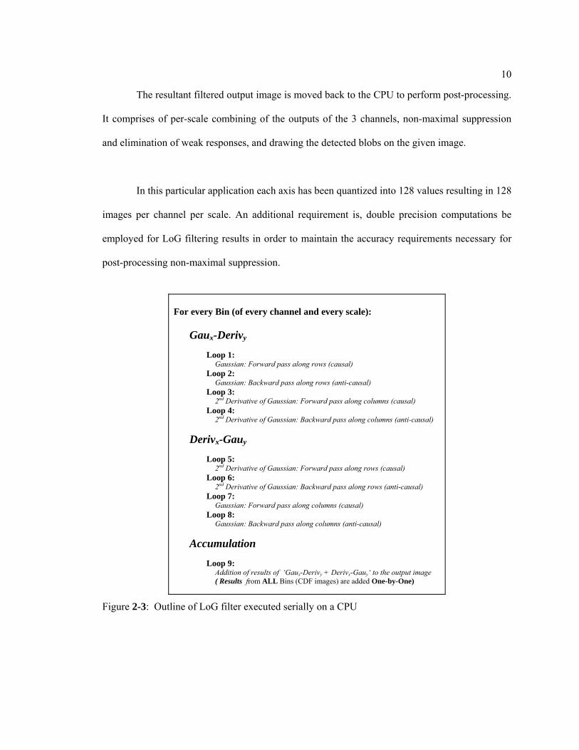
The resultant filtered output image is moved back to the CPU to perform post-processing.

It comprises of per-scale combining of the outputs of the 3 channels, non-maximal suppression

and elimination of weak responses, and drawing the detected blobs on the given image.

In this particular application each axis has been quantized into 128 values resulting in 128

images per channel per scale. An additional requirement is, double precision computations be

employed for LoG filtering results in order to maintain the accuracy requirements necessary for

post-processing non-maximal suppression.

For every Bin (of every channel and every scale):

Gaux-Derivy

Loop 1: Gaussian: Forward pass along rows (causal)

Loop 2: Gaussian: Backward pass along rows (anti-causal)

Loop 3: 2nd Derivative of Gaussian: Forward pass along columns (causal)

Loop 4: 2nd Derivative of Gaussian: Backward pass along columns (anti-causal)

Derivx-Gauy

Loop 5: 2nd Derivative of Gaussian: Forward pass along rows (causal)

Loop 6: 2nd Derivative of Gaussian: Backward pass along rows (anti-causal)

Loop 7: Gaussian: Forward pass along columns (causal)

Loop 8: Gaussian: Backward pass along columns (anti-causal)

Accumulation

Loop 9: Addition of results of ‘Gaux-Derivy + Derivx-Gauy‘ to the output image ( Results from ALL Bins (CDF images) are added One-by-One)

Figure 2-3: Outline of LoG filter executed serially on a CPU

11

The LoG filtering, from pixel binning is implemented as a set of 4th order IIR filters

arranged over nine loops. Figure 2-3 outlines the LoG filter when executed sequentially on a

CPU. The first eight loops can be arranged into two independent sections, loops 1 to 4, denoted

Gaux-Derivy (2-ways Gaussian in the X-direction, 2-ways 2nd derivative of Gaussian in Y-

direction) and loops 5 to 8, denoted Derivx-Gauy (2-ways Gaussian in the Y-direction, 2-ways 2nd

derivative in the X-direction). 2-ways mean once along axis (the causal component) and once

opposite to the axis (the anti-causal component). Both Gaux-Derivy and Derivx-Gauy

independently operate on the CDF images and their combined outputs produce a resulting LoG

filtered image. This is repeated for each CDF image and loop 9 is responsible for accumulating

all these LoG filtered images into a single filtered output image. This process is then repeated for

each channel, I1I2I3, and for all scales making CSDD a highly compute intensive algorithm.

Strict data dependence propagates from Gaussian to 2nd derivative of Gaussian in Gaux-

Derivy and from 2nd derivative of Gaussian to Gaussian in Derivx-Gauy. Thus loops 3-4(7-8) can

be executed only after loops 1-2(5-6). This requires the intermediate outputs of loops 1-2(5-6) to

be stored in the memory. Similarly the combined output of loops 3-4-7-8 need to be stored for

inputs to loop-9. This is a lot of memory requirement considering the multiple bins, scales and

axes. Another major constraint for parallelizing the LoG filter is introduced due to the recurrence

relation along rows and columns. The Deriche filter requires that during each pass, either a 5x1

(rows) or 1x5 mask (columns), operate on the current pixel and the previous four results from the

mask (eg. an = pnm0+an-1m1+an-2m2+an-3m3+an-4m4). This requires additional information to be

stored per pixel (m1, m2, m3, m4) in addition to the final output of the pass per pixel. Also thus,

the pixels in a row and column cannot be computed upon independently. The inherent

independence is limited to between rows and between columns only.

12

Figure 2-4: Inherent parallelism in LoG filtering per bin. (Every bin is also independent)

13

Figure 2-4 illustrates the inherent parallelism in the LoG filtering. Rows and columns are

shown vertical and horizontal respectively because of column-major data storage. With the

amount of data dependency (from loops 1-2(5-6) to 3-4(7-8), along rows in loops 1-2(5-6), and

along columns in loops 3-4(7-8)), CSDD is essentially not a massively parallel algorithm and is a

challenge to parallelize it on SIMD architectures with limited memory.

14

Chapter 3

GPU AND CUDA BASICS

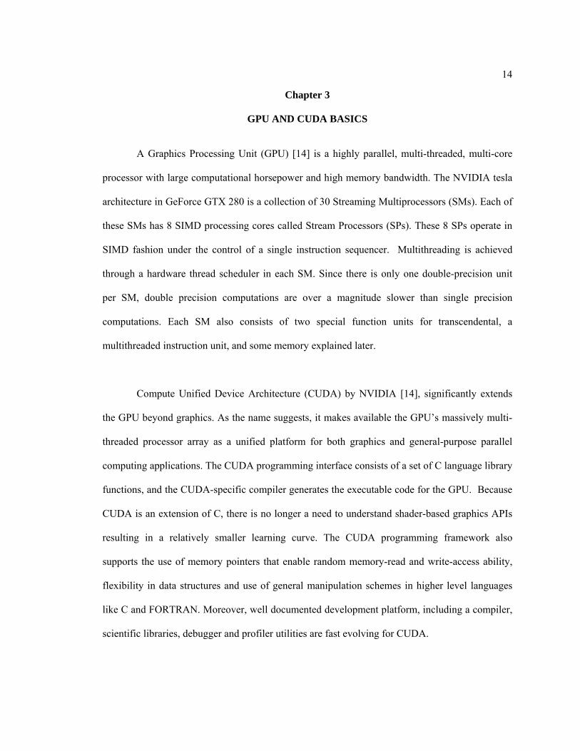
A Graphics Processing Unit (GPU) [14] is a highly parallel, multi-threaded, multi-core

processor with large computational horsepower and high memory bandwidth. The NVIDIA tesla

architecture in GeForce GTX 280 is a collection of 30 Streaming Multiprocessors (SMs). Each of

these SMs has 8 SIMD processing cores called Stream Processors (SPs). These 8 SPs operate in

SIMD fashion under the control of a single instruction sequencer. Multithreading is achieved

through a hardware thread scheduler in each SM. Since there is only one double-precision unit

per SM, double precision computations are over a magnitude slower than single precision

computations. Each SM also consists of two special function units for transcendental, a

multithreaded instruction unit, and some memory explained later.

Compute Unified Device Architecture (CUDA) by NVIDIA [14], significantly extends

the GPU beyond graphics. As the name suggests, it makes available the GPU’s massively multi-

threaded processor array as a unified platform for both graphics and general-purpose parallel

computing applications. The CUDA programming interface consists of a set of C language library

functions, and the CUDA-specific compiler generates the executable code for the GPU. Because

CUDA is an extension of C, there is no longer a need to understand shader-based graphics APIs

resulting in a relatively smaller learning curve. The CUDA programming framework also

supports the use of memory pointers that enable random memory-read and write-access ability,

flexibility in data structures and use of general manipulation schemes in higher level languages

like C and FORTRAN. Moreover, well documented development platform, including a compiler,

scientific libraries, debugger and profiler utilities are fast evolving for CUDA.

15

The CUDA core consists of three abstractions [14]: a hierarchical model of threads, a

controllable memory hierarchy, and barrier synchronization.

CUDA [14] employs a hierarchical model to organize and support a high level of

parallelism i.e. a high volume of threads running in parallel on the GPU. A thread, the finest

granularity of parallelism on the GPU, is simply a sequence of instructions that can be executed

on different data units in parallel. CUDA organizes threads into logical blocks. Because there are

a limited number of threads that a block can contain, these blocks are then organized into grids

allowing for a larger number of threads to run concurrently. A grid is usually 2D with its

dimensions specified in terms of number of blocks. Thus block ID is a 2-component vector with

each block uniquely identified within a grid using a one-dimensional or two-dimensional index.

Block dimensions are specified in terms of number of threads. Thread ID is a 3-component

vector, so that threads can be uniquely identified within a block using a one-dimensional, two-

dimensional, or three-dimensional index. All the threads in a grid are organized in identical

blocks and run the same GPU code called the Kernel (though conditional branching is possible

using unique thread and block IDs). The total number of threads is equal to the number of threads

per block times the number of blocks. Only one kernel can execute on the GPU at a time.

Execution configuration determines the number of blocks and number of threads per block

executing the kernel on the GPU. It is explicitly managed by the programmer and is specified at

the time of kernel launch. This block organization allows the algorithm to scale with future

generations of the GPU.

Each SM scheduler employs SIMT architecture to create, manage, and execute

concurrent threads in hardware with zero scheduling overhead. Thread blocks are required to

execute independently. It must be possible to execute them in any order, in parallel or in series.

16

This independence requirement allows thread blocks to be scheduled in any order across any

number of cores, enabling programmers to write scalable code. Thus all the blocks in a grid are

distributed over the SMs, with one block executing on an SM at a time. As thread blocks

terminate, new blocks are launched on the vacated multiprocessors. The threads of a thread block

execute concurrently on an SM and are time-sliced over its SPs in groups of 32 threads called a

warp. The way a block is split into warps is always the same; each warp contains threads of

consecutive, increasing thread IDs with the first warp containing thread 0. Each warp executes in

lock step and thus each SP operates on 4 threads. Every 4 cycles, the scheduler selects a warp that

is ready to execute and issues the next instruction to the active threads of the warp. A warp

executes one common instruction at a time, so full efficiency is realized when all 32 threads of a

warp agree on their execution path. If threads of a warp diverge via a data dependent conditional

branch, the warp serially executes each branch path taken; disabling (hardware masking) threads

that are not on that path, and when all paths complete, the threads converge back to the same

execution path. Branch divergence occurs only within a warp; different warps in a thread block

execute independently regardless of whether they are executing common or disjointed code paths.

Latencies are simply tolerated by switching warps. Table 3-1 lists the hardware specifications for

GTX 280. Though a very large number of threads may theoretically be possible for a GPU

(maximum number of blocks per grid x maximum number of threads per block), the hardware

limits their concurrent availability to the developer, as clipped by the maximum number of active

threads (warps or blocks) per SM.

The Tesla architecture is supports workloads with relatively small temporal data locality

and only much localized data reuse. As a consequence, it does not provide large hardware caches

shared among multiple cores, as is the case on modern CPUs. The GPU comes with a hierarchical

memory structure. Memory access times do vary for different memory levels. CUDA framework

17

provides an almost explicit control for each of these levels. This enables the fine-tuning of the

code’s data access patterns to optimize the performance. Table 3-2 lists the details on these

different memories and the issues involved if not accessed correctly.

Table 3-1 Compute specifications for compute capability 1.3 (GTX 280)

Number of Multiprocessors (SMs) 30

Number of Streaming (scalar) Processors (SPs) 8

Warp-size (Number of Threads per Warp) 32

Maximum sizes of each dimension of a Grid 65535 x 65535 x 1

Maximum sizes of each dimension of a Block 512 x 512 x 64

Texture alignment 256 Bytes

Maximum number of Active Blocks per SM 8

Maximum number of Active Warps per SM 32

Maximum number of Active Threads per SM 1024

Support for Double Precision Yes

18

Table 3-2 CUDA controllable memory hierarchy for GTX 280 Is

sues

Ser

iali

zati

on

occu

rs u

pon

un

-coa

lesc

ed

mem

ory

acce

ss

No

issu

es. B

eing

pe

r th

read

, acc

ess

is c

oale

sced

Thr

eads

of

sam

e w

arp

shou

ld r

ead

clos

ely

loca

ted

addr

esse

s

Lin

earl

y sl

ow

unti

l hal

f-w

arp

read

s fr

om th

e sa

me

loca

tion

Sam

e as

for

te

xtur

e m

emor

y

Sam

e as

for

co

nsta

nt m

emor

y

Ban

k co

nfli

cts

Ban

k co

nfli

cts

Pu

rpos

e

Sto

re k

erne

l in

puts

&

outp

uts;

Hos

t-D

evic

e, in

ter-

thre

ad /b

lock

/k

erne

l co

mm

unic

atio

n

Spa

ce f

or

regi

ster

spi

lls.

Sto

re a

rray

or

stru

ctur

ed d

ata

Bro

adca

st to

all

th

read

s in

a

War

p, S

tore

un

-str

uctu

red

data

N/A

N/A

Inte

r-th

read

co

mm

unic

atio

n w

ithi

n a

blo

ck

Aut

o-va

riab

les

Sco

pe

Glo

bal

Fun

ctio

n/ K

erne

l

Glo

bal

Glo

bal

Glo

bal

Glo

bal

Fun

ctio

n / K

erne

l

Fun

ctio

n / K

erne

l

Lat

ency

200-

400

Cyc

les

(Slo

w)

200-

400)

C

ycle

s (S

low

)

1 to

100

s of

cyc

les

base

d on

ca

che

1 to

100

s of

cyc

les

base

d on

ca

che

> R

egis

ter

Lat

ency

> R

egis

ter

Lat

ency

~ R

egis

ter

Lat

ency

Fas

test

Siz

e

1GB

Up

to G

loba

l (R

esid

es

ther

e)

Up

to G

loba

l (R

esid

es

ther

e)

Up

to G

loba

l (R

esid

es

ther

e)

64K

B (

16K

B

per

2 S

Ms)

64K

B (

8KB

pe

r S

M)

16K

B p

er

SM

16,3

84 3

2-bi

t R

egis

ters

pe

r S

M

Wh

o

All

thre

ads

&

Hos

t

One

thre

ad

(Onl

y T

hrea

d W

rite

s)

All

thre

ads

&

Hos

t (O

nly

Hos

t Wri

tes)

All

thre

ads

&

Hos

t (O

nly

Hos

t Wri

tes)

All

thre

ads,

H

ost

All

thre

ads,

H

ost

All

thre

ads

in a

bl

ock

(Onl

y T

hrea

ds W

rite

)

One

thre

ad

(Onl

y T

hrea

d W

rite

s)

Acc

-e

ss

R/

W

R/

W

R/O

R/O

R/O

R/O

R/

W

R/

W

Loc

atio

n

Off

– C

hip,

O

n-ca

rd

Off

– C

hip,

O

n-ca

rd

Off

– C

hip,

O

n-ca

rd

Off

– C

hip,

O

n-ca

rd

On

– C

hip

C

ache

On

– C

hip

Cac

he

On

– C

hip

On

– C

hip

Mem

ory

Glo

bal

Loc

al

Tex

ture

Con

stan

t

Tex

ture

C

ach

e

Con

stan

t C

ach

e

Sh

ared

Reg

iste

rs

19

GPU is employed as a co-processor. CUDA kernels are offloaded by the CPU (Host) to

execute on the GPU (Device). The CUDA software stack [14] is composed of several layers: a

compiler device driver (nvcc), an application programming interface (API) (driver and runtime),

and two higher-level mathematical libraries of common usage, CUFFT and CUBLAS, with

CUDA runtime API. CUDA runtime library is split into a host component that runs on the host

and provides functions to control and access one or more compute devices from the host; a device

component that runs on the device and provides device specific functions; and a common

component that provides a subset of the standard C library and some more built-in features that

are supported in both host and device code. CUDA assumes that both the host and the device

maintain their own DRAM, referred to as host memory and device memory, respectively. The

host component of the CUDA program manages the global, constant, and texture memory spaces

(visible to kernel) as input preparation for the kernel. This includes device memory allocation and

de-allocation, as well as data transfer between host and device memory. The shared memory and

register spaces are managed inside the CUDA kernel by the device component.

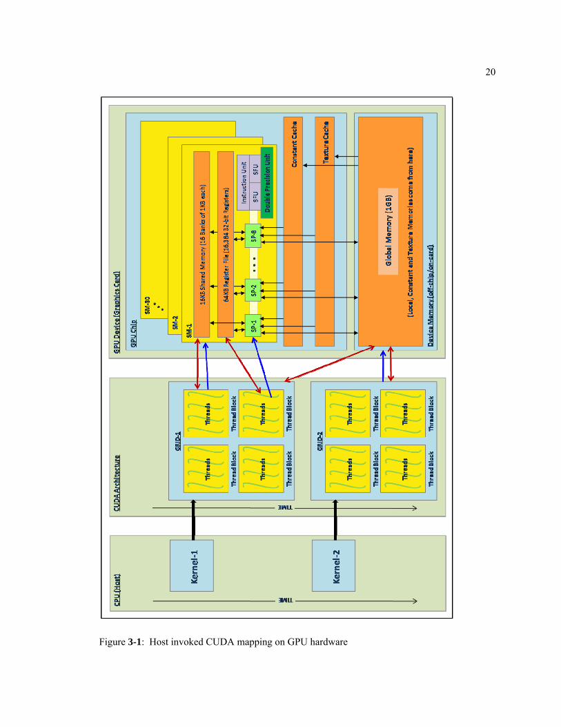
Figure 3-1 shows the host invoked mapping of CUDA onto the GPU hardware. The host

launches Kernels as grids of identical thread blocks. Different kernels are executed one after the

other. The blocks are scheduled on the SM and the threads are executed on the SPs. The figure

pictorially represents how the memory resources are distributed over the SM and how different

girds, blocks and threads communicate through different memories.

20

Figure 3-1: Host invoked CUDA mapping on GPU hardware

21

Chapter 4

IMPLEMENTATION OF CSDD ON GPU

This thesis exploits GPU capabilities for acceleration of CSDD. As shown in Figure 2-2,

only the most time consuming part, the LoG filtering, was mapped to and accelerated on the GPU

using CUDA. The GPU hardware and CUDA details are as provided in chapter 3.

4.1 CSDD Mapping on CUDA

The LoG filter is mapped on to the GPU in 3 CUDA kernels as shown in Figure 4-1.

However, as shown in Figure 4-2, the independent paths in every kernel are not executed

concurrently. Kernel-1 performs the first halves of Gaux-Derivy and Derivx-Gauy in series in the

order of loops 1, 5, 2 and 6. Kernel-2 performs the second halves of Gaux-Derivy and Derivx-Gauy

in series in the order of loops 3, 7, 4, and 8. Kernel-3 performs loop-9 by adding the outputs

(Gaux-Derivy + Derivx-Gauy) of all bins in series (one-by-one).

Considering the nature of the LoG Filtering [section 2.2], the following factors were

considered in deciding this mapping:

4.1.1. Memory requirement

The net LoG filtering in this implementation requires 128 binary images as inputs. As

shown in Figure 4-1, instead of storing 128 binary images, the threshold operation for generation

of binary value for any pixel for any bin is carried out each time it is required. Also, as shown in

Figure 4-1, the outputs per bin of loops 1 and 2 (5 and 6) are stored in the same location.

22

Similarly per bin outputs of loops 3, 4, 7 and 8 are all stored in the same location to

increase re-use of memory. These output locations form the intermediate data structures per bin

Figure 4-1: CSDD mapping on GPU (per bin) in 3 kernels

23

that keep occupying memory across kernels. Depending on the available global memory after

storing the input image and filter co-efficients, as many bins (with the intermediate data

structures) as can be accommodated are included into a single stream of kernels and the entire

histogram is completed in multiple streams. The global memory is never filled beyond 80%. LoG

filtering for each channel and each scale is always executed by a new stream (or bunch of

streams) of these 3 kernels.

For every Bin (of every channel and every scale):

KERNEL-1

Loop 1: Gaussian: Forward pass along rows (causal)

Loop 5: 2nd Derivative of Gaussian: Forward pass along rows (causal)

Loop 2: Gaussian: Backward pass along rows (anti-causal) Loop 6:

2nd Derivative of Gaussian: Backward pass along rows (anti-causal)

KERNEL-2

Loop 3: 2nd Derivative of Gaussian: Forward pass along columns (causal)

Loop 7: Gaussian: Forward pass along columns (causal)

Loop 4: 2nd Derivative of Gaussian: Backward pass along columns (anti-causal)

Loop 8: Gaussian: Backward pass along columns (anti-causal)

KERNEL-3

Loop 9: Addition of results of ‘Gaux-Derivy + Derivx-Gauy‘ to the output image ( Results from ALL Bins (CDF images) are added One-by-One)

Figure 4-2: Outline of serial execution within 3 GPU kernels

24

4.1.2. Computational requirement and Scalability with future hardware

Figure 4-3 shows the mapping of the 3 CUDA kernels as grids of thread-blocks. Since

LoG requires the input image to be computed upon over and over again for different bins of the

histogram, the number of blocks is as high as number of tiles x number of bins. Each block

computes one tile of the input image for any one of the bins. Since there are at least two

concurrent paths in LoG (Gaux-Derivy and Derivx-Gauy, and computation of causal and anti-

Figure 4-3: Mapping of 3 CUDA kernels as grids of thread-blocks

25

causal components), different blocks could be branched to perform on different independent steps

making the number of blocks equal to number of tiles x number of bins x number of concurrent

steps. However, this approach could not be followed due to reasons discussed ahead.

The scheme of tiling and availability of at least 128 blocks (over 4blocks per SM for

GTX 280) make the model scalable with future hardware. The concurrency will further increase

with the number of processing cores.

4.1.3. Bandwidth

The host to device bandwidth being limited, only the inputs and the LoG filtered output

image is transferred between the two. All intermediate data structures are created on device,

retained and computed upon across kernels, and destroyed on device without ever being mapped

by the host or copied to host memory. This may be even at the cost of increased memory usage

leading to reduced computation per kernel or low parallelism in a kernel, as in kernel-3.

4.1.4. Data dependency

Individual pixels cannot be computed upon due to row-wise and column-wise data

dependencies. The image is therefore broken down into tiles along rows or columns and assigned

to blocks with the number of threads equal to the number of rows or columns in the tile and every

thread performing serial computations along the entire row or column, respectively. Thus, the

number of tiles and threads may be different for filtering along X and Y directions. If this

happens within a kernel, it may lead to branching and resource wastage due to idling of certain

threads. Hence, as shown in Figure 4-1, operations along X direction, 1-2(5-6), are clubbed in

kernel-1 while the operations along Y direction, 3-4(7-8), are clubbed in kernel-2.

26

4.1.5. Re-use of data

The more is the re-use of the input or output data, the higher is the scope of benefiting

from cached memories or shared memory. In kernels -1 and -2, first both the causal components,

loops 1-5(3-7), are calculated followed by both anti-causals, 2-6(4-8). This is shown in Figure 4-

2. Since the input image is accessed in the same direction in loops 1-5(3-7) and in the same

direction in loops 2-6(4-8), this increases the scope of re-use of inputs.

4.1.6. Synchronization

Killing the kernel being the only reliable way of global synchronization between threads

across different blocks, steps with producer-consumer pattern (reads-after-writes) could not be

placed in a single kernel. Hence loops 1-2(5-6) are placed in kernel-1 while the following loops

3-4(7-8) are placed in kernel-2.

As shown in Figure 4-1, all the four loops in kernels -1 and -2 can logically be executed

in parallel and then their outputs can be added to the same location to increase memory re-use.

But this is not as trivial as it seems because of the synchronization limitations. In Kernel-1, loops

1 and 2(5 and 6) cannot be executed concurrently since synchronized writes to the same location

by threads of different blocks is not possible. Loops 1 and 5(2 and 6) also are not advisable to be

executed concurrently due to multiple reasons. Firstly, by executing these causal (anti-casual)

loops concurrently, there is a loss of substantial performance gain from the use of shared memory

(as we shall see ahead). Secondly, because of the fine-grained histogram, there will always be

ample blocks to keep the processors busy at any step. Hence any further increase in concurrency

doesn’t add to performance. Thus whether the serialization occurs intentionally or due to ample

number of threads running at any time to occupy all resources, it doesn’t affect the performance.

27

Intentional serialization within a kernel rather helps in packing more computation between two

kernel launches. This helps in offsetting the overhead associated with launching three kernels per

stream, especially for smaller images. Loops 1 and 6(5 and 2) though staggered in time to write to

the same location, will give inaccurate results upon concurrent execution. This is because

different blocks are scheduled randomly. Hence, as shown in Figure 4-2, all the four loops are

performed in series within kernel-1. Same is shown for kernel-2 because all loops have to be

serialized to be able to write to the same output location.

For the same reason, addition of outputs from different bins is carried out in series in

kernel-3. Thus, as shown in Figure 4-3, the number of blocks in kernel-3 is equal to the number

of tiles and is independent of the number of bins.

4.2 Execution Configuration

Execution parameters are the number of blocks per grid and the number of threads per

block executing a kernel and are explicitly managed by the programmer. Choosing execution

parameters is a matter of striking a balance between occupancy and number of active blocks per

SM for a given resource utilization per block decided by the application. Note that concurrency is

never a question for GPU as long as there are as many warps launched as the number of SMs (a

total of 30warps = 960threads for GTX 280, a very small number for most applications.

Occupancy is the ratio of the number of active warps per SM to the maximum number of

possible active warps per SM. Only one warp is scheduled at a time on an SM. Memory access

and instruction latencies are hidden by switching active warps and thus higher occupancy is

desired. Number of active warps (threads and blocks) means the number of warps that can be

28

accommodated within the resources available per SM, viz. registers and shared memory. Register

and shared memory usage are functions of algorithm design and input size. The number of

registers (and shared memory) needed per thread (and per block) decides the number of active

warps available, and in turn the occupancy. Figure 4-4 summarizes this relation between the

resources and the occupancy. The execution configuration needs to be chosen such that enough

thread blocks are created to occupy all the processing units of the GPU with maximum achievable

occupancy. However, the active threads/warps/blocks should remain below hardware limitations

specified in Table 3-1. The following discussion justifies the selection of execution configuration

(operating point) for CSDD in the region shown in Figure 4-4.

Figure 4-4: Relation between Resources required per block and Occupancy

29

4.2.1. Selecting the right occupancy

Higher occupancy does not always equate to higher performance. In fact, once occupancy

of 50% is reached, additional increases in occupancy do not translate into improved performance.

However, low occupancy always interferes with the ability to hide memory latency, resulting in

performance degradation. As shown in Figures 4-6 and 4-7, LoG filtering in CSDD is a very

memory-access intensive problem. Thus it suffers from high memory access latencies. Hence a

higher occupancy (50% or more as shown in Figure 4-4) has been maintained in all the three

kernels. This will also ensure high occupancy in future hardware with increased registers, shared

memory resources and permissible threads per block.

4.2.2. Selecting the right number of active blocks per SM

A thread block is entirely executed on an SM (and not distributed across SMs). The

number of blocks in a grid should be larger than the number of SMs so that all SMs have at least

one block to execute. But only one block per SM will force the SM to idle when the block is

waiting for thread synchronization at the __syncthreads() barrier and also during global memory

reads if there are not enough threads per block to cover the load latency. Thus there should be

multiple active blocks per SM. More thread blocks stream in pipeline fashion through the device

and amortize overhead even more. It was observed that anything below 3 active blocks per SM

caused a reduction in the CSDD performance.

4.2.3. Selecting the right number of blocks per grid

To scale to future devices, the number of blocks per kernel launch should be in hundreds.

The number of blocks for both kernels -1 and -2 is number of tiles x number of bins. As

mentioned in the CSDD mapping on CUDA [section 4.1], the fine grained histogram ensures at

30

least 128 bins at any time for both kernels -1 and -2. This ensures at least 4 blocks per SM for

GTX 280 which is highly scalable for next few generations of hardware.

4.2.4. Selecting the right number of threads per blocks

When choosing the number of threads per block (block-size), it is important to remember

that multiple active blocks can reside on an SM and so occupancy is not decided by the block-size

alone. Allocating more threads per block is better for efficient time slicing, but the more threads

per block, the fewer registers are available per thread. Thus, larger block-size does not necessarily

imply a higher occupancy. On the other hand, having less number of threads per block increases

the number of blocks. But this will aid the occupancy only till the upper limit on either the

number of active warps or the number of active blocks per SM (Table 3-1) is not reached. Thus,

achieving the right number of active threads with given per SM resources will also decide the best

execution configuration. This required a lot of experimentations explained ahead.

The number of threads per block is recommended to be a multiple of warp-size (32

threads) to avoid wasting compute resources on under populated warps and to facilitate coalesced

memory accesses. But the only way to avoid register memory bank conflicts is to have the

number of threads per block a multiple of 64, which is the warp allocation granularity for

registers. The latency of register read-after-write dependencies is approximately 24 cycles and is

completely hidden on SMs that have at least 192 active threads (i.e., 6 warps). This equates to

6/32 = 18.75% occupancy and hence is taken care of in any grid size for all the kernels except for

kernel-3 if the image dimensions are less than 192x192. Thus 64, 128, 192, 256, 320 and so on

seem to be good numbers for threads per block provided enough registers and shared memory

resources are available. Figure 4-5 shows the effect on performance when the block-size is not a

31

multiple of 32 or 64. The execution times with multiple of 64 block-sizes have been normalized

to 1 to be able to cover a range of times.

The LoG implementation requires a maximum of 26 registers per thread. The –

maxrregcount cannot be set for individual kernels. After some experimentation with cost of

local memory access (due to force reduction in number of registers) versus benefits of

occupancy (in terms of performance), the flag “–maxrregcount” was set to 20 for all the 3

kernels. As explained in the following section on optimizations, the amount of dynamically

allocated shared memory is directly proportional to the number of threads per block. Thus a

higher number of threads per block may prohibit higher occupancy. Block sizes of 64, 128, 192

and 256 threads were arrived at after experimentation for occupancy (considering given

registers and, statically allocated shared memory) and its impact on performance. The

details are explained ahead with reference to Table 4-1.

Figure 4-5: Relative performance with block-sizes multiples and non-multiples of 64

0.920.940.960.98

11.021.041.061.081.1

1.121.14

240x380 600x600 800x600 1600x1200

Relative

 Execution Tim

es

Image Size (Note: Images are further padded for block‐sizes that are multiples of 64)

Relative Execution Times for different block‐sizes

Block‐size a non‐multiple of 64

Block‐size a multiple of 64

32

For the blob-detection system to be able to handle images of all sizes, the dimensions

need to be padded to the nearest multiple of the right block-size (64, 128, etc). MATLAB’s

identical paddarray feature is used to pad the image dimensions with identical pixels as those at

the corresponding edge (boundary). The most obvious approach is to launch the block sizes as per

the padded image dimensions and then by-pass the padding during computation. But this would

introduce branching in the logic and would also lead to idling of certain threads almost per block.

On the other hand no branching would introduce errors. Hence experimentations on accuracy

vs. different padding sizes were carried out. It was observed that padding of up to 64 rows and

columns of pixels on any edge (i.e. a total of up to 127 rows or columns of padding) could be

handled with adequate accuracy without introducing conditional branching. But this would mean

a lot of extra work by the GPU as compared to the CPU. Experimentations on performance vs.

different padding sizes were made. It was observed (Table 4-1) that even with as low as 64

threads per block; the occupancy remained above 50% without affecting the performance

(acceleration). Hence the padding was limited to up to a total of 63 (i.e. 32 on any edge). This

further justified the use of as low as 64 threads per block.

Most of the above experiments were aided by the CUDA Occupancy calculator. Table 4-

1 shows the analysis of occupancy considerations in selection of the right block-size. Shared

memory allocation details have been discussed ahead in the section 4.3 on optimizations. Beyond

256 threads per block, the number of active blocks per SM reduces to 2 or less. Also there is a

marginal reduction in performance, perhaps due to reasons discussed in 4.2.2 above. Since CSDD

is highly memory access intensive and since there is no performance benefit in having large

block-size, the highest number of threads per block is clipped at 256. Figure 4-4 shows the

execution configuration for CSDD lying in the region marked with occupancy > 50%, the number

of active blocks per SM > 2, and minimum 64 threads per block.

33

Table 4-1 Considerations in selection of right block-size

Krnl

# Threads

per Block

#Regi-sters per

thread

lmem access (Bytes)

per thread

Static shared

memory (Bytes)

per block

Dynamic shared

memory (Bytes)

per block

% Occupancy

# Active Warps

(Blocks)per SM

Limited by

1 64 20 16 368 256 50 16 (8) Max warps per SM

2 64 20 80 368 256 50 16 (8) Max warps per SM

3 64 8 0 64 256 50 16 (8) Max warps per SM

1 128 20 16 368 512 75 24 (6) Registers per SM

2 128 20 80 368 512 75 24 (6) Registers per SM

3 128 8 0 64 512 100 32 (8) Max warps per SM

1 192 20 16 368 768 75 24 (4) Registers per SM

2 192 20 80 368 768 75 24 (4) Registers per SM

3 192 8 0 64 768 94 30 (5) Max warps per SM

1 256 20 16 368 1024 75 24 (3) Registers per SM

2 256 20 80 368 1024 75 24 (3) Registers per SM

3 256 8 0 64 1024 100 32 (4) Max warps per SM

1 320 20 16 368 1280 63 20 (2) Registers per SM

2 320 20 80 368 1280 63 20 (2) Registers per SM

3 320 8 0 64 1280 94 30 (3) Max warps per SM

1 384 20 16 368 1536 75 24 (2) Registers & Max

Warps per SM

2 384 20 80 368 1536 75 24 (2) Registers & Max

Warps per SM

3 384 8 0 64 1536 75 24 (2) Max warps per SM

1 512 20 16 368 2048 50 16 (1) Registers per SM

2 512 20 80 368 2048 50 16 (1) Registers per SM

3 512 8 0 64 2048 100 32 (2) Max warps per SM

Note: Multiples of 64 have been chosen for block-size based on post-padding accuracy and performance considerations discussed before. Resource (registers and shared memory) usage comes from the code. Considerations of register pressure (-maxrregcount 20) have also been discussed before. As shown in Figure 4-4, Occupancy > 50% and Active Blocks per SM > 2 are desired.

34

The implementation automatically picks up the right block size so as to limit the net

amount of padding to 63 rows or/and columns of pixels with maximum (of 64, 128, 192 and 256)

threads possible per block. Image dimension divided by the number of threads per block gives the

number of tiles per bin perpendicular to that dimension. Table 4-2 shows the image padding for

various image sizes.

Table 4-2 Image padding for various image sizes

Image Size #

Streams

Threads per Block

along Rows

Threads per Block

along Columns

Padding in height (#Rows)

Padding in width (#Cols)

Image Size on GPU

#Rows #Cols #Rows #Cols

320 240 1 64 256 0 16 320 256 240 380 1 256 192 16 4 256 192 512 256 1 256 256 0 0 512 256 576 512 2 192 256 0 0 576 512 480 640 2 256 128 32 0 512 640 512 768 2 256 256 0 0 512 768 800 600 2 64 128 32 40 832 640 768 768 4 256 256 0 0 768 768

1280 1024 8 256 256 0 0 1280 1024 1600 1200 8 64 64 0 16 1600 1216

4.3 Optimizations and their Impacts

After all the above considerations (in sections 4-1 and 4-2), the only major optimization

left to be explicitly applied to the implementation is the use of low-access-latency memories.

Since all the four steps in kernels -1 and -2 are being executed in series, there is no concurrent re-

use of the input images by threads of different blocks and/or by threads of the same block. Thus

use of read-only cached memories like texture and constant is futile. Moreover, these being read-

only memories, they can be put to only specific use. As reflected from Table 4-1, shared memory

35

per SM is not a limiting factor for any block-size configuration. Thus even shared memory

remains under-utilized owing to the nature of the algorithm.

In all the three kernels, the Gaussian and Derivation filter coefficients and other constants

are pulled into the shared memory once per kernel and are re-used extensively. This reduces the

time by up to 15% in spite of introducing divergence and warp serializations due to branching

within warp (caused due to idling of the threads in the warp not used in this loading). However,

no more than half a warp gets employed at any time to load these co-efficients and constants into

shared memory. Thus the shared memory bank conflicts cannot happen in spite of many of these

being double precision. The static shared memory allocation in Table 4-1 comes from these

constants pulled into shared memory and arguments to __global__ functions (kernels) also stored

in the shared memory.

In kernel-1, first the starting row of the input image is pulled into the shared memory and

is re-used twice (at the beginning of loops 1 and 5 for generating the first row of the binary CDF

image). Then the last row of the input image is pulled into the shared memory and is re-used

twice (at the beginning of loops 2 and 6 for generating the last row of the binary CDF image).

This is because causal and anti-causal components start accessing the input image from the

beginning and the end respectively. This causes an additional improvement of 35%. Every

location in the output of kernel-2 is being written to four times, twice by Gaux-Derivy and twice

by Derivx-Gauy. First, every location of the output is pulled into the shared memory, and after it is

written to twice (by causal components of Gaux-Derivy and Derivx-Gauy), it is updated in the

global memory. Thereafter, every location of the output is again pulled into the shared memory,

and after it is written to twice (by anti-causal components of Gaux-Derivy and Derivx-Gauy), it is

updated in the global memory. Since all the 4 loops have to be performed in series and since

36

direction of computations change for loops 4 and 8, it is not possible that each location be pulled

into shared memory once and re-used four times. This improves the performance of kernel-2 by

another 25%. In kernel-3, every location of the output image is being written to once every bin.

Hence every location of the output image is pulled into the shared memory, and only after the

thread adds the corresponding location from all the bins into that shared memory location, it is

updated in the global memory. This improves the performance of kernel-3 by around 25%.

Kernels -2 and -3 see reduced performance gain compared to kernel-1. This is because kernels -2

and -3 use shared memory for writing to the output (unlike reading from the input as in kernel-1).

Since this use of shared memory changes with the block-size, it is dynamically decided and

allocated at the time of kernel-launch based on the block-size (listed under dynamic shared

memory allocation column in Table 4-1).

The net improvement in the implementation performance due to use of shared memory is

around 30% for most image sizes. Figures 5-2 and 5-3 show the improvement in the

implementation and application speed-ups with use of shared memory. Though LoG filtering

requires double precision due to non-maximal suppression, the input and output images and the

shared memory computations (except constants and coefficients) are being handled with single

precision accuracy. This prevents shared-memory bank-conflicts. Input image being used only for

threshold comparisons (for generation of binary CDF images), it could be handled in single

precision without loss in accuracy in kernel-1. Fortunately, adequate accuracy could be

maintained till the final output in spite of the single precision computations for the outputs in

kernels -2 and -3.

37

Figure 4-6: Profiler counters for optimized GPU execution

Figure 4-7: Break-up of overall execution time on the GPU

0%

10%

20%

30%

40%

50%

60%

70%

80%

90%

Kernel‐1 Kernel‐2 Kernel‐3 Memcpy

Profiler counters for optimized GPU execution (768x768 Image)

% of total GPU time

gst coalesced

gld coalseced

local store

local load

instructions

branch

divergence

warp serialization

0%

10%

20%

30%

40%

50%

60%

70%

80%

90%

Kernel‐1 Kernel‐2 Kernel‐3 Memcpy

Break‐up of overall execution time on the GPU(768x768 image)gst coalesced

gld coalseced

local store

local load

instructions

38

Figure 4-6 illustrates the performance profile for the final optimized versions of the 3

kernels. The profiling results are shown for a square image for a fair comparison between kernels

-1 and -2. As is seen, kernel-2 takes the largest portion of the CSDD execution time on GPU

largely contributed by memory accesses (global and local). As seen in Figure 4-7, all the three

kernels spend a significant portion of their execution time on memory accesses. Thus memory

access latencies are the major bottleneck for even the optimized implementation.

Since the kernel-2 takes the maximum time on GPU due to memory accesses, in case of

rectangular images the preprocessing rotates the input image such that kernel-2 does lesser serial

execution per thread than kernel-1. When the larger dimension is fed to Kernel-2 as the number

of columns, there are more threads in kernel-2 than kernel-1 and they perform on lesser number

of pixels per column (since number of rows = pixels per column < number of columns). The net

LoG filtered output is again rotated, but in the opposite direction, so as to map to the original

input image. This optimization exploits the rotational invariance property of the CSDD algorithm

to give up to 14% performance improvement due to reduced memory accesses.

A basic strategy followed throughout the implementation is to avoid conditional

branching as much as possible. This was achievable also because of the structured image access

patterns at every loop in the LoG filtering. The indexing logic is devised such that any thread in

any kernel will always access the same memory location when operating in a particular direction.

The direction changes are taken care of by a number of ways: separating X and Y direction

computations in kernels -1 and -2; serial execution of all 4 loops in both kernels -1 and -2;

executing the causal components of both Gaux-Derivy and Derivx-Gauy first and followed by the

anti-causal components of both Gaux-Derivy and Derivx-Gauy (allowing time for thread

synchronization between direction changes); use of shared memory locations and __syncthreads()

39

barrier to ensure a series of writes to the same location by multiple threads and porting only the

final result to the global memory. Thus there can neither be any conflict between threads while

writing to the same location not can there be any branching and serialization. This claim is

reinforced by the profiler results in Figures 4-6 and 4-7. The contribution of branching,

divergence and warp serialization to the execution time is negligible for all the three kernels. This

negligible contribution comes from adding of constants in shared memory in all the three kernels

by less than a warp of threads. Branching is relatively higher because of 9 different loops

involved (manifesting as manifold nested loops in the code). It was measured upon profiling that,

the dynamically allocated shared memory did not contribute towards any divergence and

serialization due to bank conflicts. This reinforces the claim made earlier about use of single

precision for computations involving shared memory.

Also, the indexing logic makes extensive use of modulo division and division. These

being expensive operations, multiple occurrences of them are reduced to just once per thread by

calculating the binID and tileID for every thread in the beginning of the kernel. These IDs

thereafter remain constant across the kernel.

If a variable located in global or shared memory is declared as volatile, the compiler

assumes that its value can be changed at any time by another thread and therefore any reference

to this variable compiles to an actual memory read instruction. Thus, use of volatile __shared__

variables to limited extent leads to reduced use of register (or local memory) variables for

temporary results. Using volatile __shared__ variables is as fast as using registers, assuming there

are no shared memory bank conflicts. Unless the variable is declared as volatile, the compiler

optimizes the reads and writes to shared memory (provided __syncthreads() is used to ensure

writes). After some experimentation with different (read-only after being loaded once)

40

__shared__ variables declared as volatile, the local memory access was reduced by 8Bytes in

kernel-1 giving an additional 1% improvement in performance.

A major trade-off was made by choosing considerations of scalability over 3-5%

performance improvement. Looking at various GPU generations, we see that there has been a

doubling in the number of registers per SM over generations while the amount of shared memory

per SM has remained the same across all generations. Permissible number of active blocks per

SM has also doubled over generations. As seen in Table 4-1, shared memory remains under-

utilized while registers remain over-burdened for almost all configurations. Hence some of the

register burden was offloaded to shared memory by creating 2-3 block-size length of shared

memory arrays for 2-3 local variables. Any location of any array would store the corresponding

local variable for the thread indexing to that location. This scheme gave 3-5% performance

improvement when 3 4-bytes local variables from kernel-1 and 2 4-bytes local variables from

kernel-2 were offloaded from registers to shared memory. 4-bytes variables were chosen to

prevent shared memory bank conflicts. This improvement came from nearly 50% reduction in the

total local memory accesses by kernels -1 and -2. This maintained the same occupancy on GTX

280 for all block-sizes listed in Table 4-1. However, for most block-sizes, the shared memory

utilization reached saturation (i.e. number of active warps got limited by shared memory as well).

This may inhibit scalability with future generations if the shared memory per SM doesn’t increase

while. Hence this 3-5% performance improvement was foregone and not implemented in the final

system.

Other minor recommendations have been followed all through the code. Example, all

type-conversions are done explicitly (especially between float and double), etc. There was no

scope of using fast math and many other optimizations recommended by NVIDIA. Loop

41

unrolling called for extra registers and did not add to any performance gain. There is hardly any

branching for branch predication to be applied. Stream processing using asynchronous operations

did not work in this scheme. Since LoG filtering for all bins needs to be carried out in multiple

streams for bigger images due to lack of global memory, there was never enough memory to

overlap kernel execution and memcpy of two different streams. The pyramid approach suggested

in [7] for hot-spot computations was applied to kernel-3 to increase concurrency and reduce the

extent of global synchronization required. However as observed in [7], it decreased the

performance due to idling of resources (when reduction applied in the same kernel) and due to

increased overhead of kernel launches (when reduction applied over a series of kernels). Also in

either scheme, there being no scope of use of shared memory, the performance only reduced.

Another  thought was  to perform kernel‐3 on  the CPU and  free  the GPU  to execute kernels  ‐1 

and  ‐2  of  the  next  stream  simultaneously. However,  kernel-3 execution on the CPU required

moving the entire output of kernel-2 back to CPU in every stream costing 10% additional time.

Hence there was no other option for kernel-3. As shown in figures 4‐6 and 4‐7, data transfer per 

stream between host and device is limited to less than 1%. 

4.4 Accuracy

As mentioned before, non-maximal suppression in the post-processing requires higher

accuracy than delivered by single precision computations on the GPU. Hence double precision

GPU computations had to be employed. The only way to determine the “required” accuracy or

rather permissible loss of precision by GPU was to compare the visual outputs of the GPU with

respect to the CPU. During the course of the development of this implementation, the visual

outputs of the two were compared with every new optimization or CUDA provision introduced.

42

Table 4-3 Comparison of saliency detection by CPU and GPU

CPU: 480x640 grey-scale image. Blobs detected for 1 channel and 19 scales, at an average of 15.3secs for net LoG filtering per channel per scale.

GPU: 512x640 (with padding) grey-scale image. Blobs detected for 1 channel and 19 scales, at an average of 1.3secs for net LoG filtering per channel per scale. The image was also rotated for computations on GPU.

CPU: 517x725 grey-scale image. Blobs detected for 1 channel and 19 scales, at an average of 19.4secs for net LoG filtering per channel per scale.

GPU: 576x768 (with padding) grey-scale image. Blobs detected for 1 channel and 19 scales, at an average of 1.7secs for net LoG filtering per channel per scale. The image was also rotated for computations on GPU.

CPU: 450x300 colored image. Blobs detected for 3 channels and 17 scales, at an average of 11.9secs for net LoG filtering per channel per scale.

GPU: 512x320 (with padding) colored image. Blobs detected for 3 channels and 17 scales, at an average of 0.78secs for net LoG filtering per channel per scale.

43

The final implementation largely employs double precision computations with exceptions

of most shared memory computations. The liberty of using single precision at intermediate steps

was taken only till identical outputs were available from CPU and GPU for all images for all

scales. Based on the visual results it was quantified that an accuracy of at least four places after

decimal was required at the output of net LoG filtering by the GPU. Table 4-3 shows the visual

outputs of saliency detection from CPU and GPU for a few sample images. Identical blobs are

detected for all kinds of grayscale as well as colored images.

4.5 Parameterization for Scalability on Future Hardware

The blob-detection system implemented and accelerated using GPU should be able to

scale over future increases in hardware resources on the GPU without additional engineering

costs. This requires the execution configuration and few other quantities to be parameterized

based on few of the relevant GPU hardware parameters from Table 3-1.

4.5.1. Global Memory

Based on the parameter GLB_MEM (to represent the available Global Memory), the pre-

processing decides the number of streams (STREAM_QTY) and the histogram granularity per

stream (BIN_QTY_PER_STREAM) required to execute the LoG implementation on the GPU for

a given image. No more than 80% of the global memory is filled up.

4.5.2. Number of SMs and SPs

These do not affect the scalability of the model. As mentioned earlier, 128 bins ensure up

to 4 Blocks per SM on GTX 280 and performance should remain relatively unhampered with up

to double the number of SMs (i.e. up to 2 Blocks per SM) provided that there will be enough

44

memory to accommodate all the bins in a single stream. It seems obvious that the limits on

maximum number of active warps and blocks per SM (LIMIT_ACTIVE_WARPS_PER_SM, and

LIMIT_ACTIVE_BLOCKS_PER_SM) will also increase with increased number of processing

cores causing a linear scale-up in the speed-up as long as enough occupancy is maintained to

overcome latencies.

4.5.3. Warp-size

NVIDIA claims that the warp-size of 32 will not change for generations of GPU to come

and hence this factor will not affect the scalability. Nevertheless, a parameter WARP_SIZE has

been introduced such that it takes care of increase in warp-size till warp allocation granularities

for registers and shared memory remain greater or equal to 1.

4.5.4. Execution Configuration (Grid and Block sizes)

The GRID_SIZE for each kernel has been parameterized as function of the histogram

granularity per stream, and the input image size (BIN_QTY_PER_STREAM x TILE_QTY).

As explained earlier, for any dimension (height for kernel-1 and width for kernel-2) of an

input image, the largest possible BLOCK_SIZE requiring minimum padding is selected from a

range of block-sizes (64, 128, 192 and 256 for the current implementation on GTX 280). The

range of these block-sizes is MIN_BLOCK_SIZE, 2 x MIN_BLOCK_SIZE, 3 x

MIN_BLOCK_SIZE, till MAX_BLOCK_SIZE = n x MIN_BLOCK_SIZE.

As seen before, the CSDD implementation requires certain minimum OCCUPANCY,

and minimum number of active blocks per SM (ACTIVE_BLOCKS_PER_SM). The current

implementation also fixes the register requirement per thread (RGSTRS_USED_PER_THREAD),

45

and shared memory requirement per block (SHRD_MEM_USED_PER_BLOCK). Hence the only

parameters that can change the BLOCK_SIZE with hardware generations are

LIMIT_RGSTRS_PER_SM, LIMIT_SHRD_MEM_PER_SM, LIMIT_ACTIVE_WARPS_PER_SM,

and LIMIT_ACTIVE_BLOCKS_PER_SM. Therefore, MIN_BLOCK_SIZE and

MAX_BLOCK_SIZE are computed based on these parameters in the following way:

1. The limit on the minimum block-size (MIN_BLOCK_SIZE) is computed as the maximum

of the warp allocation granularity for registers and for shared memory.

_ _ max _ _ _ ,

_ _ _ _ x _

It is then checked for active blocks per SM and occupancy. Kernel-2 being the most

compute and resource intensive, it is ok to check for kernel-2 alone. Occupancies of kernels -

1 and -3 will always be either equal or more.

_ _ _ 2

ACTIVE_BLOCKS_PER_SM x MIN_BLOCK_SIZE

_ _ _ _ x _50%

If the above checks are not cleared, MIN_BLOCK_SIZE is fixed at 64.

2. The pre-processing continuously raises the upper limit on the block-size for this application

(MAX_BLOCK_SIZE) to the next multiple of MIN_BLOCK_SIZE till the following are

achieved for kernel-2:

46

_ _ _ 2

ACTIVE_BLOCKS_PER_SM x MAX_BLOCK_SIZE

_ _ _ _ x _50%

3. For reference, first let’s look at how the actual number of active blocks per SM is decided for

a given block size:

a. Physical limit on the number of active Blocks per SM (Table 3-1):

_ _ _ _

b. Physical limit on the number of Warps per SM:

floor _ _ _ _

BLOCK_SIZE / _

c. Limited by registers available per SM (LIMIT_RGSTRS_PER_SM):

floor _ _ _

_ _ _ x BLOCK_SIZE

d. Limited by shared memory available per SM (LIMIT_SHRD_MEM_PER_SM):

floor _ _ _ _

SHRD_MEM_USED_PER_BLOCK

floor _ _ _ _

_ _ _ _ _ 4 x BLOCK_SIZE

Hence the maximum number of active blocks with a given BLOCK_SIZE will be:

_ _ _ min a, b, c, d

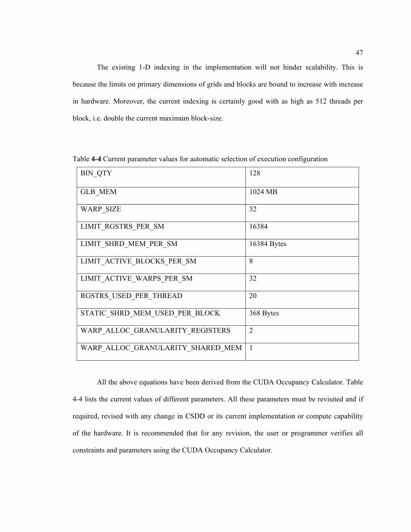
47

The existing 1-D indexing in the implementation will not hinder scalability. This is

because the limits on primary dimensions of grids and blocks are bound to increase with increase

in hardware. Moreover, the current indexing is certainly good with as high as 512 threads per

block, i.e. double the current maximum block-size.

Table 4-4 Current parameter values for automatic selection of execution configuration

BIN_QTY 128

GLB_MEM 1024 MB

WARP_SIZE 32

LIMIT_RGSTRS_PER_SM 16384

LIMIT_SHRD_MEM_PER_SM 16384 Bytes

LIMIT_ACTIVE_BLOCKS_PER_SM 8

LIMIT_ACTIVE_WARPS_PER_SM 32

RGSTRS_USED_PER_THREAD 20

STATIC_SHRD_MEM_USED_PER_BLOCK 368 Bytes

WARP_ALLOC_GRANULARITY_REGISTERS 2

WARP_ALLOC_GRANULARITY_SHARED_MEM 1

All the above equations have been derived from the CUDA Occupancy Calculator. Table

4-4 lists the current values of different parameters. All these parameters must be revisited and if

required, revised with any change in CSDD or its current implementation or compute capability

of the hardware. It is recommended that for any revision, the user or programmer verifies all

constraints and parameters using the CUDA Occupancy Calculator.

48

Chapter 5

RESULTS

This system takes in a variety of sizes of frames, square and rectangular, as inputs. It also

takes in colored images. However the results here are limited to gray-scale images consisting of a

single channel. The only implication of limiting this discussion to gray-scale is that the LoG

filtering execution time for 3-channel images is three times as large (for both CPU and GPU).

The overall speedup remains relatively unchanged.

Figure 5-1 depicts the overall application time of the CSDD implementation on both the

CPU and GPU for selected image sizes. Even after using an optimized CPU code, the algorithm

still requires anywhere from several seconds to a few minutes for a single frame. Considering 3-

channels, the execution time can be anywhere from 7~10 minutes for a single frame of larger

dimensions. The GPU however, improves upon this time significantly, consistently achieving

Figure 5-1: Execution times of Overall CSDD application on CPU and GPU

0.000

20.000

40.000

60.000

80.000

100.000

120.000

140.000

160.000

180.000

320x240 480x640 512x768 1280x1024 1600x1200

Time (s)

Image Size

Execution Time of CSDD using CPU and GPU

CPU

GPU w/o SM

GPU w/ SM

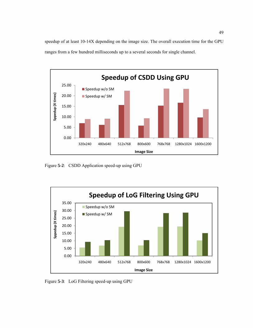
49

speedup of at least 10-14X depending on the image size. The overall execution time for the GPU

ranges from a few hundred milliseconds up to a several seconds for single channel.

Figure 5-2: CSDD Application speed-up using GPU

Figure 5-3: LoG Filtering speed-up using GPU

0.00

5.00

10.00

15.00

20.00

25.00

320x240 480x640 512x768 800x600 768x768 1280x1024 1600x1200

Sppedup (X tim

es)

Image Size

Speedup of CSDD Using GPU

Speedup w/o SM

Speedup w/ SM

0.00

5.00

10.00

15.00

20.00

25.00

30.00

35.00

320x240 480x640 512x768 800x600 768x768 1280x1024 1600x1200

Sppedup (X tim

es)

Image Size

Speedup of LoG Filtering Using GPU

Speedup w/o SM

Speedup w/ SM

50

Figure 5-2 shows the overall CSDD application speed-up using GPU. Figure 5-3 shows

the LoG filtering speed-up using GPU. In a few instances the GPU is able to improve upon the

CPU execution time by up to 30X. In particular this occurs with images with dimensions as

multiples of 256. This increase in speedup is actually due to an increase in the CPUs execution

time due to increased cache miss behavior when the data is being accessed column-wise and the

cache-line spatiality benefit is not being harnessed. The data being stored in column-major

fashion, loops 1-5-2-6 (kernel-1) access memory column-wise to access the image row-wise.

Thus, as shown in Figure 5-4, these loops take the most time. 256 being the cache-line size and a

power of 2, the problem is scaled taking around 3X more time. Upon profiling the CPU code for

hardware counters using PAPI (Performance Application Programming Interface), it was seen

that L1 cache misses increase by 1.5 times while L2 cache misses increase by around 9 times in

loops 1-5-2-6 (kernel-1) when the image dimensions are multiples of 256. This issue on the CPU

can be corrected by either storing a rotated input image as well or by padding the image by

another row or/and column of pixel. However, the GPU being the central idea for this work, these

corrections have not been implemented on the CPU. Also this could possibly be a general

problem with most image processing algorithms. Thus it was useful to discover it along the

course of this thesis.

Another interesting observation is that the dominant kernel changes from the CPU to

GPU implementation. Figure 5-4 shows the break-up of the times spent on different kernels by

the CPU. Kernel-1 takes the majority time on the CPU. Figure 5-5 shows the break-up of the

times spent on different kernels by the GPU. Contrary to as shown in Figure 5-4, kernel-2 takes

the majority time on the GPU. There being no caching, there are no caching related differences

between kernels -1 and -2 on the GPU. As can be explained from Figures 4-6 and 4-7, kernel-2

51

has manifold global and local memory accesses than kernel-1 on the GPU causing it to take up

the majority of the overall execution time.

Figure 5-4: Break-up of time spent by different kernels on the CPU

Figure 5-5: Break-up of time spent by different kernels on the GPU

0

50

100

150

200

250

300

Time (s)

Image Size

Kernel Execution Time (CPU)

Kernel 3

Kernel 2

Kernel 1

0

1

2

3

4

5

6

7

8

Time (s)

Image Size

Kernel Execution Time (GPU w/ SM)

Kernel 3

Kernel 2

Kernel 1

52

Chapter 6

CONCLUSION

CSDD is a unique feature extraction and matching algorithm that works well on textured

and natural images, and also performs very well under large changes of scale and in-plane

rotation.

Most accelerators are SIMD in nature, suffer from memory access as bottleneck, and are

best compared for massively parallel problems. Thus CSDD becomes a good candidate for

comparison of these accelerators for not-so massively parallel problems. This thesis is pioneering

in a way that it well exploits the capabilities and limitations of GPUs for a data-intensive as well

as data-dependent problem like CSDD and presents a highly scalable parallel programming

model for the application that can work efficiently and accurately on all image sizes. With better

hardware resources (like faster memories and more double precision units) or with CUDA

provision of Global Synchronization, the application shows promise to perform at real-time

speeds.

With the current GPU and CUDA provisions falling short in achieving real-time speeds

for the amount of data and computation involved in CSDD, benchmarking CSDD on IBM Cell

may be a good proposition for future work.

53

Appendix

TIPS ON TOOLS AND ENVIRONMENT SET-UP

There are many tools used in the entire process of CSDD implementation on the GPU.

Some of them are well documented and trivial to use but most are not because of lack of proper

documentation. They are either poorly documented or not documented at all by even NVIDIA.

Most information is scattered unstructured over multiple resources. This appendix compiles few

tips and directions on all such tools under one chapter of this thesis. They have been gathered

over the entire course of this research, either after lot of trials and errors or after extensive

searching on the internet. Thus this appendix will be a good reference for future users.

1. CUDA TOOLKIT – Download this from the NVIDIA website for specific version of CUDA

and install it. This sets up the basic environment for CUDA programming.

2. CUDA API – NVIDIA CUDA Programming Guide [14] for the specific CUDA version is

the best resource to learn about using CUDA API. NVIDA website also provides many other

supporting documents and tutorials that prove very useful. NVIDIA CUDA Forums are the

best place to look for information on programming practices and less developed or un-

documented CUDA provisions. Developers are more than happy to discuss your issues and

answer your queries.

3. CUDA SDK – CUDA SDK is the best demonstration of the use of CUDA API. The

deviceQuery.cu sample program queries and gives the hardware specifications of the GPU(s)

on the system. Other useful programs (for versions higher than CUDA 2.0) for querying

additional hardware data are cudaGetDeviceProperties.cu and canMapHostMemory.cu.

54

4. CUDA Occupancy Calculator – Extensive use of CUDA Occupancy Calculator is explained

in sections 4.2 and 4.5 of this thesis. This can be downloaded from the NVIDIA CUDA

website.

5. NVMEX – NVMEX is the MATLAB plug-in for CUDA that helps in calling a CUDA

function from MATLAB. The lone document available on NVMEX from NVIDIA doesn’t

suffice for all the information required to be able to use it. This thesis uses MATLAB for

image pre-processing, CUDA for the LoG implementation, C for non-maximal suppression

and again MATLAB for the rest of the post-processing. Hence NVMEX was employed. The

various aspects related to the use of NVMEX are listed as follows:

5.1 C function can be treated with either NVMEX as below or with standard MEX. This

implementation uses NVMEX to compile both CUDA and C portions of the project.

5.2 Download the CUDA plug-in for MATLAB for the specific CUDA version from the

NVIDIA website. Right now it comes as a collection of files in a folder. The README

in there only describes how to run the test codes using NVMEX. To set up the

environment for NVMEX, copy the files nvmexopts.bat, nvmex.m and nvmex_helper.m

in the folder Files\MATLAB\R2008a\bin\win32\mexopts. nvmexopts.bat is the NVIDIA

CUDA equivalent of mexopts.bat used for MEX.

5.3 Modify this copy of nvmexopts.bat to include all the compiler options required for LoG

implementation. The changes need to be made in the compiler parameters only.

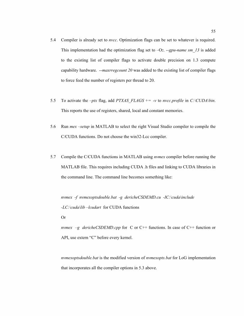
55

5.4 Compiler is already set to nvcc. Optimization flags can be set to whatever is required.

This implementation had the optimization flag set to –O2. --gpu-name sm_13 is added

to the existing list of compiler flags to activate double precision on 1.3 compute

capability hardware. --maxrregcount 20 was added to the existing list of compiler flags

to force feed the number of registers per thread to 20.

5.5 To activate the –ptx flag, add PTXAS_FLAGS += -v to nvcc.profile in C:\CUDA\bin.

This reports the use of registers, shared, local and constant memories.

5.6 Run mex –setup in MATLAB to select the right Visual Studio compiler to compile the

C/CUDA functions. Do not choose the win32-Lcc compiler.

5.7 Compile the C/CUDA functions in MATLAB using nvmex compiler before running the

MATLAB file. This requires including CUDA .h files and linking to CUDA libraries in

the command line. The command line becomes something like:

nvmex -f nvmexoptsdouble.bat -g dericheCSDEMD.cu -IC:\cuda\include

-LC:\cuda\lib –lcudart for CUDA functions

Or

nvmex –g dericheCSDEMD.cpp for C or C++ functions. In case of C++ function or

API, use extern “C” before every kernel.

nvmexoptsdouble.bat is the modified version of nvmexopts.bat for LoG implementation

that incorporates all the compiler options in 5.3 above.

56

6. CUDA Emulator – The CUDA function can be compiled in emulation mode by following

all the above steps with only one difference. Create a copy of nvmexoptsdouble.bat as

nvmexoptsemuldouble.bat with -c -deviceemu added at the beginning of the DEBUGFLAGS

under compiler parameters. Use nvmexoptsemuldouble.bat in the command line instead of

nvmexoptsdouble.bat. This allows using all features possible in the emulation mode including

debugging using Visual Studio. However, emulation on windows is not possible beyond

30,000 threads since that is the limit on the number of POSIX threads that can be created on

windows.

7. Debugging using Visual Studio in Emulation Mode – No CUDA documentation is

available on this (one can find documentation on gdb and Linux though). Compile the CUDA

portions of the project in MATLAB in emulation mode as described above. Open visual

Studio and select Tools → Attach to Process → MATLAB.exe. Open the C/CUDA file and

place break-points as needed. Run the MATLAB file for the project and the control will

break at the break-point. However limited Visual Studio provisions are available during

debugging, unlike debugging of general C/C++ program using Visual Studio. Debugging in

MATLAB can happen irrespective of whether the C/CUDA function has been compiled in

emulation or execution mode. This is because the MATLAB portion is anyways running on

the CPU and not on the GPU.

8. CUDA Visual Profiler – NVIDIA CUDA Visual Profiler is a very useful tool for

performance profiling of CUDA functions on the GPU. Version 1.1.08 was used for this

implementation. The use of this profiler first requires setting the environment variables in the

system. Go to Control Panel → System → Advanced → Environment Variables and set

CUDA_PROFILE to 1 in both User variables and System variables. Now compile the CUDA

57

function in MATLAB using nvmex. Then open the Visual Profiler and click on Session

settings. While running the profiler for a stand-alone CUDA program, the launch path is

expected to be a visual studio CUDA project executable. With NVMEX, set launch to

MATLAB i.e. C:/Program Files/MATLAB/R2008a/bin/win32/MATLAB.exe. Working

directory is the one in which the nvmex compiled .cu file lies. Set the Arguments to –r <name

of the .m file to run the project, without .m extension> (e.g. –r CSDD). Set the Max.

Execution Time to a sufficiently large value, say 3000secs. In other tabs of Session settings,

you can check all profiler counters (instead of 4 at a time) and all options at once. The only

difference will be, with more than 4 counters selected, the profiler will automatically perform

multiple runs to sample the selected counters (instead of we running it multiple times to

measure 4 different counters per run). With each run, the profiler will launch a MATLAB

session. Keep manually closing each MATLAB session as it ends. With these instructions,

the profiler is all set to be used. If command line profiler is to be used instead of visual

profiler, CUDA_PROFILE_CSV or CUDA_PROFILE_LOG could be set to 1 in both User

variables and System variables. Similarly, set CUDA_PROFILE_CONFIG to

cuda_profiler.conf in the working directory (e.g. C:\CSDD\cuda_profiler.conf) in both User

variables and System variables. Place the cuda_profiler.conf file in the working directory and

specify the counters to be measured. This would give the counters in the .csv or .log file

respectively. How to use various visual profiler provisions and interpret the results is very

well explained in the profiler README document. The environment variables can also be set

from the CUDA Visual Profiler → Options → Environment Variable Settings.

9. Syntax Highlighting for .cu file in Visual Studio – Use the resource in C:\Program

Files\NVIDIA Corporation\NVIDIA CUDA SDK\doc\syntax_highlighting. The readme file

there in has all the details on the needful. 

58

REFERENCES

1. R. T. Collins and W. Ge, "CSDD Features: Center-Surround Distribution Distance for

Feature Extraction and Matching," in European Conference on Computer Vision

(ECCV), Marseille, France, October 2008.

2. R. Deriche, "Fast algorithms for low-level vision," in 9th International Conference on

Pattern Recognition, vol. 1, 1988, pp. 434-438.

3. G. Farneback and C.-F. Westin, "Improving Deriche-style Recursive Gaussian Filters,"

Journal of Mathematical Imaging and Vision, vol. 26, no. 3, pp. 293-299, Dec. 2006.

4. Y. Allusse, P. Horain, A. Agarwal, and C. Saipriyadarshan, "GpuCV: an opensource

GPU-accelerated framework for image processing and computer vision," in International

Multimedia Conference, Vancouver, British Columbia, Canada, 2008, pp. 1089-1092.

5. N. Courty and P. Hellier, "Accelerating 3d Non-rigid Registration Using Graphics

Hardware," International Journal of Image and Graphics (IJIG), vol. 8, no. 1, pp. 81-98,

Jan. 2008.

6. D. Castano-Diez, D. Moser, A. Schoenegger, S. Pruggnaller, and A. S. Frangakis,

"Performance evaluation of image processing algorithms on the GPU," Journal of

Structural Biology, vol. 164, no. 1, pp. 153-160, Oct. 2008.

59

7. S. Che, et al., "A performance study of general-purpose applications on graphics

processors using CUDA," Journal of Parallel and Distributed Computing, vol. 68, no. 10,

pp. 1370-1380, Oct. 2008.

8. KM Hou, A. Belloum, M. Meribout, “A perception sensor for mobile robot,” Real-time

Imaging, vol. 3, pp. 379–90, 1997.

9. L. Torres, E. Bourennane, M. Robert, M. Paindavoine, “A Recursive Digital Filter

Implementation for Noisy and Blurred Images,” in Real Time Imaging Journal, vol. 4, no

3, pp. 181-191, June, 1998.

10. L. Kessal, N. Abel, D. Demigny, “Real-time image processing with dynamically

reconfigurable architecture,” Real-Time Imaging, vol. 9, 297–313, 2003.

11. E G. Lorca, L. Kessal, and D. Demigny, “Efficient asic and fpga implementations of iir

filters for real time edge detection,” in Proc. International Conference on Image

Processing (IEEE ICIP), no. 2, pages 406-409, Santa Barbara, October 1997.

12. E. Levina, P. Bickel, “The earth mover’s distance is the Mallows distance: Some insights

from statistics,” in International Conference on Computer Vision, vol. II, pp. 251–256,

2001.

13. Y. Ohta, T. Kanade, T. Sakai, “Color information for region segmentation,” Computer

Graphics and Image Processing, vol. 13, pp. 222–241, 1980.

60

14. NVIDIA. (2008, Jun.) NVIDIA CUDA. [Online].

http://developer.download.nvidia.com/compute/cuda/2_0/docs/NVIDIA_CUDA_Progra

mming_Guide_2.0.pdf