A Generalized Approach to Planar InductionHeating Magnetics

by

Richard Yi Zhang

B.E. (Hons), University of Canterbury, New Zealand (2009)

Submitted to the Department of Electrical Engineering and ComputerScience

in partial fulfillment of the requirements for the degree of

Master of Science

at the

MASSACHUSETTS INSTITUTE OF TECHNOLOGY

June 2012

c© Massachusetts Institute of Technology 2012. All rights reserved.

Author . . . . . . . . . . . . . . . . . . . . . . . . . . . . . . . . . . . . . . . . . . . . . . . . . . . . . . . . . . . . . . . .Department of Electrical Engineering and Computer Science

May 18, 2012

Certified by. . . . . . . . . . . . . . . . . . . . . . . . . . . . . . . . . . . . . . . . . . . . . . . . . . . . . . . . . . . .John G. Kassakian

Professor of Electrical Engineering and Computer ScienceThesis Supervisor

Accepted by . . . . . . . . . . . . . . . . . . . . . . . . . . . . . . . . . . . . . . . . . . . . . . . . . . . . . . . . . . .Leslie A. Kolodziejski

Chair, Department Committee on Graduate Theses

2

A Generalized Approach to Planar Induction Heating

Magnetics

by

Richard Yi Zhang

Submitted to the Department of Electrical Engineering and Computer Scienceon May 18, 2012, in partial fulfillment of the

requirements for the degree ofMaster of Science

Abstract

This thesis describes an efficient numerical simulation technique of magnetoquasistaticelectromagnetic fields for planar induction heating applications. The technique isbased on a volume-element discretization, integral formulation of Maxwell’s equa-tions, and uses the multilayer Green’s function to avoid volumetric meshing of theheated material. The technique demonstrates two orders of magnitude of computa-tional advantage compared to existing FEM techniques. Single-objective and multi-objective optimization of a domestic induction heating coil are performed using thenew technique, using more advanced algorithms than those previously used due to theincrease in speed. Both optimization algorithms produced novel, three-dimensionalinduction coil designs.

Thesis Supervisor: John G. KassakianTitle: Professor of Electrical Engineering and Computer Science

3

4

Acknowledgments

My work would not have been possible without the mentorship of my advisor, Prof.

John G. Kassakian. My deepest gratitude to Prof. Kassakian for his guidance and

support, and for providing me the environment to pursue my interests.

Much of the numerical foundations of this work resulted from helpful discussions

with Prof. Jacob K. White, who kindly and patiently shared his insights with me.

I am grateful to Yang Wang of The Vollrath Company for her industry perspec-

tives, and for supporting the experimental portions of my work. I would also like to

thank Laurent Jeanneteau of Electrolux Major Appliances Europe for our extensive

conversations.

My MIT experience has been greatly shaped by the friends I have made over the

past two years at Ashdown, in EECS, the GSC and the Energy Club. I would like to

thank all of my officemates for our interesting and insightful conversations, as well as

our spontaneous technical discussions. I would like to thank my girlfriend Amy for

making everything so much fun.

Finally, I am forever indebted to my parents for all the sacrifices they have made

for me throughout my life.

The financial support of the William Georgetti Charitable Trust and the John R

Templin Scholarship Trust are gratefully acknowledged.

5

6

Contents

1 Introduction 13

1.1 Motivation . . . . . . . . . . . . . . . . . . . . . . . . . . . . . . . . . 13

1.2 Proposed Method . . . . . . . . . . . . . . . . . . . . . . . . . . . . . 16

2 The Induction Heating Process 17

2.1 Equivalent Circuit Model . . . . . . . . . . . . . . . . . . . . . . . . . 17

2.2 The MQS Electromagnetic Formulation . . . . . . . . . . . . . . . . . 19

2.2.1 Mutual Impedance . . . . . . . . . . . . . . . . . . . . . . . . 20

2.2.2 Skin and Proximity Effect Losses . . . . . . . . . . . . . . . . 22

2.3 Analytical Methods . . . . . . . . . . . . . . . . . . . . . . . . . . . . 22

2.4 Numerical Methods . . . . . . . . . . . . . . . . . . . . . . . . . . . . 25

2.4.1 Domain methods . . . . . . . . . . . . . . . . . . . . . . . . . 25

2.4.2 Integral methods . . . . . . . . . . . . . . . . . . . . . . . . . 25

2.5 The Partial Element Equivalent Circuit (PEEC) Method and FastHenry 26

3 The PEEC Planar Induction Heating Field Model 29

3.1 The Multilayer Green’s Function Approach to Eddy Currents . . . . . 30

3.2 Derivation of the Multilayer Green’s functions . . . . . . . . . . . . . 34

3.2.1 The Dyadic Green’s Function for the Semi-Infinite Half-Space 35

3.2.2 The Dyadic Green’s function Multiple-Layered Configuration . 39

3.2.3 Application of Numerical Hankel Transforms . . . . . . . . . . 46

3.3 Evaluation of the Modified Green’s Function via Quadrature . . . . . 47

3.4 Eddy Current Loss Profile . . . . . . . . . . . . . . . . . . . . . . . . 51

7

3.4.1 Theoretical Basis . . . . . . . . . . . . . . . . . . . . . . . . . 52

3.4.2 Implementation Details . . . . . . . . . . . . . . . . . . . . . . 53

3.5 Comparison to Previous Analytical Models . . . . . . . . . . . . . . . 54

3.5.1 Acero et al. . . . . . . . . . . . . . . . . . . . . . . . . . . . . 55

3.5.2 The effect of discretization . . . . . . . . . . . . . . . . . . . . 55

3.6 Experimental Validation . . . . . . . . . . . . . . . . . . . . . . . . . 57

3.7 Performance . . . . . . . . . . . . . . . . . . . . . . . . . . . . . . . . 64

4 Optimal Design of an Induction Cooktop 67

4.1 The Fitness Function . . . . . . . . . . . . . . . . . . . . . . . . . . . 68

4.1.1 Encoding Algorithm . . . . . . . . . . . . . . . . . . . . . . . 68

4.1.2 The Electromagnetic Model . . . . . . . . . . . . . . . . . . . 69

4.1.3 Scoring Algorithm . . . . . . . . . . . . . . . . . . . . . . . . 70

4.2 Single-Objective Optimization of Temperature Profile . . . . . . . . . 73

4.3 Multi-Objective Optimization of Temperature, Efficiency and Cost . . 78

5 Conclusions and Future Work 83

8

List of Figures

1-1 Illustration of an induction cooktop . . . . . . . . . . . . . . . . . . . 14

2-1 Lumped parameter transformer model for an induction heating system 17

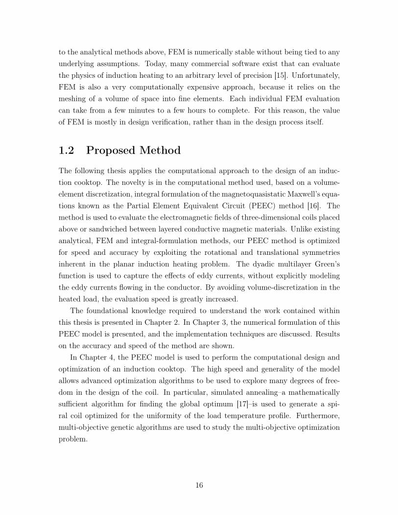
2-2 Four-element model for an induction heating system. . . . . . . . . . 18

2-3 Illustration of the Dodd and Deeds two-conductor plane system . . . 23

2-4 The circular filament approximation of the circular spiral . . . . . . . 24

3-1 Geometries of the point current source above a semi-infinite surface . 36

3-2 Geometry of the point current source within the multilayered configu-

ration . . . . . . . . . . . . . . . . . . . . . . . . . . . . . . . . . . . 40

3-3 Comparison between our filament model and measurements by Acero

et al. . . . . . . . . . . . . . . . . . . . . . . . . . . . . . . . . . . . . 56

3-4 The relative errors of our filament model . . . . . . . . . . . . . . . . 57

3-5 Comparison between the circular filament exact solution and results

generated by piecewise linear discretization . . . . . . . . . . . . . . . 58

3-6 Relative errors of the piecewise linear approximation of the circular

filament . . . . . . . . . . . . . . . . . . . . . . . . . . . . . . . . . . 59

3-7 Dimensions of the measured litz wire coil . . . . . . . . . . . . . . . 61

3-8 Measurements of the coil terminal impedance with and without the load 62

3-9 Comparison of experimentally measured coil impedances with simu-

lated results . . . . . . . . . . . . . . . . . . . . . . . . . . . . . . . . 63

4-1 Series resistance for a loop of wire of different constructions . . . . . . 71

4-2 Finite difference method stencil of the thermal system . . . . . . . . . 73

9

4-3 Original coil used as the starting point of the optimization analysis . 75

4-4 Improved coil after 2500 simulated annealing optimization iterations . 75

4-5 Improved coil at the end of the hybrid pattern search . . . . . . . . . 76

4-6 Comparison of the heat and temperature profiles of the designs . . . . 76

4-7 Heat and Temperature profiles of the three designs in 3D . . . . . . . 77

4-8 Comparison of single-objective optimized coil designs . . . . . . . . . 79

4-9 Results from multi-objective optimization with the NSGA-II Genetic

Algorithm . . . . . . . . . . . . . . . . . . . . . . . . . . . . . . . . . 81

4-10 Comparison of multi-objective optimized coil designs . . . . . . . . . 82

10

List of Tables

3.1 Speed benchmark of the axial-symmetric formulation. . . . . . . . . . 64

3.2 Speed benchmark of the 3D Formulation . . . . . . . . . . . . . . . . 65

3.3 Comparison of mutual impedance computation speeds with established

PEEC tools . . . . . . . . . . . . . . . . . . . . . . . . . . . . . . . . 66

11

12

Chapter 1

Introduction

In domestic applications, induction heating is most commonly found as the inductioncooktop (see Figure 1-1). Unlike traditional flame- or element-based appliances, theinduction cooktop heats its vessel directly by the use of a varying magnetic field.This magnetic field is generated within the cooktop by a flat spiral work coil, in turndriven by a high frequency power inverter connected to an ac supply. A temperedglass spacer is used to physically separate the work coil and associated electronicsfrom the corrosive kitchen environment above, and also to protect the work coil fromthe heat of the cooking vessel. Electromagnetic shielding is usually placed belowthe work coil (not shown) to reduce the radiated magnetic flux, and to enhance themagnetic coupling between the coil and the vessel [1].

Induction cooktops offer several distinct advantages for the culinary end userswhen compared to traditional cooking appliances. By avoiding the use of hot heatingelements, inflammable gases and open flames, induction cooktops are safer and easierto clean. Thermal inertia is reduced, and this allows their power outputs to beadjusted and controlled with great precision. Moreover, their high energy efficiencylowers energy costs and can considerably abate ambient heating to the rest of thekitchen.

1.1 Motivation

The design of the induction coil at the heart of the cooktop is a crucial but com-plicated process, because it lies at the crossroads of circuit theory, electromagnetismand thermal physics. A great coil design must balance several competing design con-siderations, including its cost of manufacture, its compatibility with the associatedpower electronics, its efficiency and the temperature profile of its associated load:

13

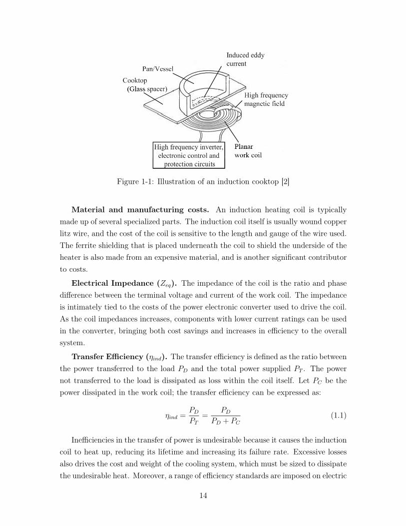
Figure 1-1: Illustration of an induction cooktop [2]

Material and manufacturing costs. An induction heating coil is typicallymade up of several specialized parts. The induction coil itself is usually wound copperlitz wire, and the cost of the coil is sensitive to the length and gauge of the wire used.The ferrite shielding that is placed underneath the coil to shield the underside of theheater is also made from an expensive material, and is another significant contributorto costs.

Electrical Impedance (Zeq). The impedance of the coil is the ratio and phasedifference between the terminal voltage and current of the work coil. The impedanceis intimately tied to the costs of the power electronic converter used to drive the coil.As the coil impedances increases, components with lower current ratings can be usedin the converter, bringing both cost savings and increases in efficiency to the overallsystem.

Transfer Efficiency (ηind). The transfer efficiency is defined as the ratio betweenthe power transferred to the load PD and the total power supplied PT . The powernot transferred to the load is dissipated as loss within the coil itself. Let PC be thepower dissipated in the work coil; the transfer efficiency can be expressed as:

ηind =PDPT

=PD

PD + PC(1.1)

Inefficiencies in the transfer of power is undesirable because it causes the inductioncoil to heat up, reducing its lifetime and increasing its failure rate. Excessive lossesalso drives the cost and weight of the cooling system, which must be sized to dissipatethe undesirable heat. Moreover, a range of efficiency standards are imposed on electric

14

appliances in some parts of the world, and the transfer efficiency of the inductioncooktop must be specially designed for these markets.

Heating and Temperature Profile. The heating profile describes the distri-bution of power output over the bottom of the heated pan, and the temperatureprofile describes the distribution of steady-state temperature over the pan. These arethe criteria that determine the quality of the cooking experience, and therefore areimportant proxies for consumer satisfaction.

Achieving a balance between all of these considerations is an exercise in multi-objective optimization. With the development of advanced computing technologies,computational design techniques have been applied to a wide range of multi-objectiveengineering optimizations problems. Regardless of the details, the core idea is toreplace the laborious and time intensive task of design by educated guesses and carefulexperimentation with a systematic process automated by a computer. In particular,two vital tasks are performed on the computer, at speeds many orders of magnitudefaster than those previously obtainable:

1. The intermediate experimental verification step, where successive iterations ofdesign are analyzed and assessed, is replaced by a software numerical optimiza-tion model.

2. Educated trial-and-error is replaced by numerical optimization algorithms thatsystematically explore the design space for better designs.

Compared to conventional design by experimental verification, computational tech-niques can analyze and assess many more designs in a span of time, without incurringextensive costs in prototyping. For these reasons, the computational design approachis found in a wide range of engineering applications, from the design of structures tocommunications and electronic devices [3, 4].

However, the computational design approach has mostly elluded domestic induc-tion heaters [5], due to the absence of the most vital ingredient – a fast and accuratecomputational technique. While fast analytical models of planar induction heatingphysics have existed since 1968 [6, 7, 8, 9, 10, 11, 12], a large collection of assumptionsare necessary for these analytical solutions to exist, such as rotational symmetry, lin-earity, isotropy, homogeneity. These assumptions limit the predictive power of themodels and the degree of freedom available to the designer. For these reasons, theusefulness of the analytical models is restricted to a limited set of conventional designs.

In more recent years, the finite element method (FEM) has become a favoredanalysis tool for the design of domestic induction heating coils [13, 14]. In comparison

15

to the analytical methods above, FEM is numerically stable without being tied to anyunderlying assumptions. Today, many commercial software exist that can evaluatethe physics of induction heating to an arbitrary level of precision [15]. Unfortunately,FEM is also a very computationally expensive approach, because it relies on themeshing of a volume of space into fine elements. Each individual FEM evaluationcan take from a few minutes to a few hours to complete. For this reason, the valueof FEM is mostly in design verification, rather than in the design process itself.

1.2 Proposed Method

The following thesis applies the computational approach to the design of an induc-tion cooktop. The novelty is in the computational method used, based on a volume-element discretization, integral formulation of the magnetoquasistatic Maxwell’s equa-tions known as the Partial Element Equivalent Circuit (PEEC) method [16]. Themethod is used to evaluate the electromagnetic fields of three-dimensional coils placedabove or sandwiched between layered conductive magnetic materials. Unlike existinganalytical, FEM and integral-formulation methods, our PEEC method is optimizedfor speed and accuracy by exploiting the rotational and translational symmetriesinherent in the planar induction heating problem. The dyadic multilayer Green’sfunction is used to capture the effects of eddy currents, without explicitly modelingthe eddy currents flowing in the conductor. By avoiding volume-discretization in theheated load, the evaluation speed is greatly increased.

The foundational knowledge required to understand the work contained withinthis thesis is presented in Chapter 2. In Chapter 3, the numerical formulation of thisPEEC model is presented, and the implementation techniques are discussed. Resultson the accuracy and speed of the method are shown.

In Chapter 4, the PEEC model is used to perform the computational design andoptimization of an induction cooktop. The high speed and generality of the modelallows advanced optimization algorithms to be used to explore many degrees of free-dom in the design of the coil. In particular, simulated annealing–a mathematicallysufficient algorithm for finding the global optimum [17]–is used to generate a spi-ral coil optimized for the uniformity of the load temperature profile. Furthermore,multi-objective genetic algorithms are used to study the multi-objective optimizationproblem.

16

Chapter 2

The Induction Heating Process

Induction heating traces its origins to the very early days of electromagnetism. Heat-ing by eddy currents was first discovered in 1865 by Leon Foucault, while experiment-ing with a rotating copper disc placed inside a permanent magnetic field. The firstpractical attempts at induction heating dates back to 1891, and the theoretical basiswas established by the luminaries of electrical engineering, including Hertz, Heaviside,Thomson, Ewing and others [18].

2.1 Equivalent Circuit Model

While its physics are strictly governed by Maxwell’s equations, the electrical proper-ties of induction heating are more easily understood in the context of an equivalentcircuit model. One common approach is to model the magnetic interaction betweenthe excited induction coil and the load as that of a standard transformer [8]. Theequivalent circuit for such a model is shown in Figure 2-1.

The lumped circuit elements included here are the primary coil resistance RC ,

Figure 2-1: Lumped parameter transformer model for an induction heating system[8]

17

Figure 2-2: Four-element model for an induction heating system.

leakage inductance Ll, magnetizing inductance Lm, turns ratio N and the load resis-tance RD. When a voltage Vp is applied to the terminals of the induction coil, primarycurrent Ip flows into the coil, inducing a voltage across Ll and Lm, but also causingsome losses to occur due to the presence of RC . The voltage induced across Lm istransformed N:1 steps down, where it appears as a voltage across the load resistanceRD. With some minor algebra, the transfer efficiency ηind can be expressed in termsof the lumped parameter component values:

ηind =RR

RR +RC (1 +R2R/X

2m)

(2.1)

Here, RR = N2RD is the resistance of the load reflected to the primary. It can beseen that the transfer efficiency is solely determined by the load resistance, windingresistance, and the magnetizing impedance.

A simpler but less physically intuitive approach used by domestic induction heat-ing researchers is to model the induction heating system as the series connection oftwo resistors and two inductors [1, 19, 20] (shown in Figure 2-2). Here, the values R0

and L0 are the resistance and inductance of the primary coil in free-space, and thevalues ∆R and ∆L are the changes in terminal resistance and inductance due to thepresence of the load. It is readily shown that this model is related to the previousmodel by the following equations:

R0 = RC (2.2)

∆R =N2RD

1 + (RR/ωLm)2(2.3)

L0 + ∆L = Ll +Lm

1 + (ωLm/RR)2(2.4)

With the four-element model, the transfer efficiency is reduced to a simple relation

18

between the two resistances:ηind =

∆R

R0 + ∆R(2.5)

It is clear from this relation that improvements in efficiency will come from an increasein ∆R or a reduction in R0.

Delving deeper into the circuit elements will require an understanding of the elec-tromagnetic field interactions that allow induction heating to occur. In particular,the parameters L0, ∆L and ∆R are the resultant of the magnetic coupling that existbetween the coil and the load. The foundational formulation of Maxwell’s Equationsare derived in Section 2.2, and a brief introduction to the modeling of magnetic cou-pling via mutual impedances is given in Section 2.2.1. The value of R0 also becomesstrongly affected by electromagnetic fields at higher frequencies, due to the skin andproximity effect; these effects are discussed in Section 2.2.2.

2.2 The MQS Electromagnetic Formulation

Maxwell’s equations solely govern the physics of practical induction heating, but themagnetoquasistatic (MQS) approximation is often used to reduce their complexity.In the conditions where frequencies rarely exceed a few hundred kilohertz, the MQSform of Maxwell’s equations is able to predict electromagnetic fields to high precision[21].

Maxwell’s equations have the following form for linear, homogenous and isotropicmedia under MQS conditions:

∇×B = µJ (2.6)

∇× E = − δ

δtB (2.7)

The simplification made by the MQS assumption is to set both displacementcurrent δD/δt and volumetric free charge ρf to zero. The physical interpretationof this is that all parasitic capacitances are neglected. The assumption allows themagnetic potential vector A to be defined with the Coulomb gauge as:

∇×A = B (2.8)

∇ ·A = 0 (2.9)

Combining (2.6)-(2.9) yields the well-known diffusion Helmholtz equation for time-

19

harmonic MQS systems:∇2A = jωµσA− µJsrc (2.10)

The right hand side of the equation describes the currents that flow within the system,and the left hand side describes the magnetic fields that are generated by thesecurrents. The first term on the right accounts for the induced eddy currents; thepresence of A in this term highlights its causal relationship with the system magneticfields. Clearly eddy currents will not flow if a material is non-conductive (σ = 0) orcompletely diamagnetic (µ = 0), and under these conditions this particular term isreduced to zero. The second term on the right accounts for the source currents thatare impressed upon the system, i.e. the currents in the coil.

For a system excited with a current Jsrc, equation (2.10) can be solved with a widerange of numerical and analytical tools to give A fields at all points in the system.The magnetic field H and the magnetic flux density B can be solved by applying thedefinition equation of the magnetic vector potential (2.8), and the electric field E canbe obtained by applying Faraday’s law (2.7):

E = −jωA (2.11)

H =1

µ∇×A (2.12)

Thus, for a given geometry of filaments and materials, the electromagnetic fieldsof the system are fully characterized once the A fields are characterized. Numericaltechniques for calculating the A fields are discussed further in Section 2.4.

2.2.1 Mutual Impedance

In circuit theory, the mutual impedance concept quantifies the coupling between theotherwise isolated elements in a circuit. In MQS systems where capacitances arezero, mutual impedance exists between different current-conducting elements due tothe magnetic coupling between them. When current flows through a conductor, amagnetic field is created according to Ampere’s law (2.6), and this magnetic field inturn induces an electric field according to Faraday’s law (2.7). If a second conductoris placed within this electric field, then a voltage is induced across this conductoraccording to:

V =

ˆcontour

E · ds (2.13)

20

Here, the line integration takes place along the contour of the second conductor.Themutual impedance Zm (with units of Ohms or Ω) is defined to be the ratio betweenthe voltage induced across the second conductor and the current that flows throughthe first conductor, i.e. for conductors 1 and 2:

Zm =1

I1

ˆcond2

E1 · ds (2.14)

I1 is the current through conductor 1, E1 is the electric field induced by conductor 1,and the integration is performed along the contour of conductor 2. Due to the reci-procity of electromagnetism, the mutual impedance of the two conductors is alwaysequal, regardless of the order of excitation and integration. It is interesting to notethat each of the conductors also exhibits mutual impedance with itself. This effect isnamed the self-impedance, but is more commonly known simply as the impedance ofthe conductor.

The self- and mutual-impedance concepts are used in induction heating to calcu-late the terminal impedance of the induction coil. In the four-element model of Figure2-2, the total terminal impedance of the coil is equivalent to the self-impedance ofcoil, in the presence of the load. To calculate this value, the coil is excited with aknown current to produce a magnetic field that induces eddy currents in the loadaccording to the diffusion Helmholtz equation (2.10). This changing magnetic fieldinduces an electric field according to Faraday’s law (2.7). The voltage induced acrossthe coil can then be measured by a line integral along the contour of the coil accordingto (2.13). Here, the integrand contains contributions to the electric field generatedby both the coil as well as the induced eddy currents in the load.

However in most realistic cases, the line integral along the contour of the coil canbe difficult to solve, and the geometry of the coil may not have an associated closed-form expression. In these cases, the calculation can be simplified by subdividing thecoil into a collection of linear filaments. The self- and mutual- impedance of andbetween each of these filaments can be separately evaluated, by exciting one pieceof the coil at a time and performing the integration independently for each filament.Since the filaments are connected in series, these self- and mutual- impedances of eachcomponent filament can be summed together to result in the self-impedance of thecombined coil.

It is important to note that each linear piecewise filament by itself does not form acomplete loop, and the resultant field that it produces does not satisfy all of Maxwell’sequations. Therefore, the impedances associated with the piecewise filaments can-

21

not be considered in the same sense as closed-loop impedances. In literature, theseimpedances are often referred to as partial impedances, to distinguish them from loopimpedances.

The calculation process for the transformer model shown earlier in Figure 2-1 isrelated but not identical to the procedure described above. An extensive discussion onhow the magnetizing inductance Lm, leakage inductance Ll, and the load impedanceRD of Figure 2-1 are related to the mutual impedances of the filaments can be foundin [8].

2.2.2 Skin and Proximity Effect Losses

The skin and proximity effects are names for the tendency of high frequency electriccurrents to distribute themselves at the outer surfaces of conductors. Because of theseeffects, the effective resistance of the conductors tend to increase dramatically at highfrequencies and also become frequency dependent. The effects stem from opposingeddy currents induced by magnetic fields, in turn a resultant of the currents thatflow within the wires. When the magnetic field is self-induced by the same conductorexperiencing the eddy currents, the increase in effective resistance is known as theskin effect. When the source of the magnetic field are external elements in proximityto the conductor, the effect is known as the proximity effect.

The skin and proximity effects can adversely affect the transfer efficiency of theinduction system according to (2.5). For the loss of efficiency to be controlled andcontained, one common technique is to use wires with strands that are individuallyinsulated from each other. The term litz wire is used to describe a special kind ofstranded wire, carefully woven in a pattern that minimizes the skin and proximity ef-fects. Due to their high frequency and high efficiency requirements, the vast majorityof domestic induction coils are wound with stranded or litz wire [1]. Thorough math-ematical models have been developed in literature to study the frequency-dependentresistances of plain and litz wires [20, 22, 23].

2.3 Analytical Methods

Many of the first investigators of induced eddy currents came from the related fieldsof non-destructive eddy current testing and from microelectronics, and analyticalsolutions had been derived for convenient symmetries. The first analytical solutionof the planar eddy current problem is often credited to Dodd and Deeds [6]. In

22

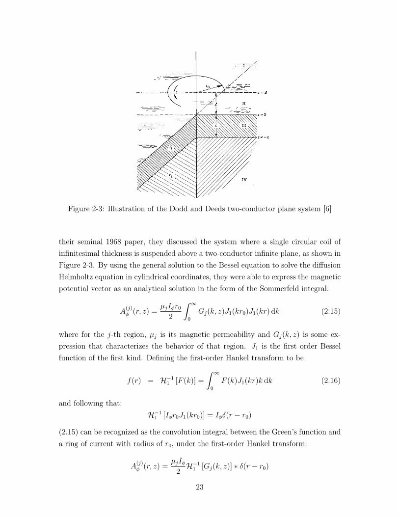
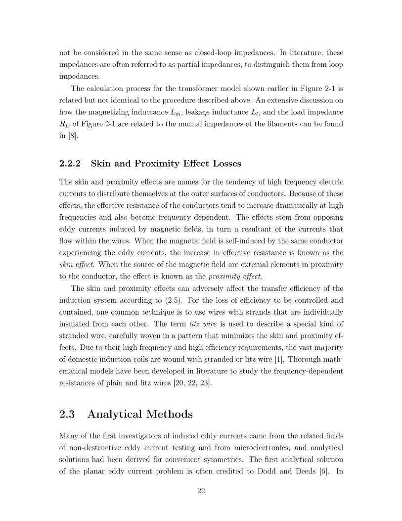
Figure 2-3: Illustration of the Dodd and Deeds two-conductor plane system [6]

their seminal 1968 paper, they discussed the system where a single circular coil ofinfinitesimal thickness is suspended above a two-conductor infinite plane, as shown inFigure 2-3. By using the general solution to the Bessel equation to solve the diffusionHelmholtz equation in cylindrical coordinates, they were able to express the magneticpotential vector as an analytical solution in the form of the Sommerfeld integral:

A(j)φ (r, z) =

µjIφr0

2

ˆ ∞0

Gj(k, z)J1(kr0)J1(kr) dk (2.15)

where for the j-th region, µj is its magnetic permeability and Gj(k, z) is some ex-pression that characterizes the behavior of that region. J1 is the first order Besselfunction of the first kind. Defining the first-order Hankel transform to be

f(r) = H−11 [F (k)] =

ˆ ∞0

F (k)J1(kr)k dk (2.16)

and following that:H−1

1 [Iφr0J1(kr0)] = Iφδ(r − r0)

(2.15) can be recognized as the convolution integral between the Green’s function anda ring of current with radius of r0, under the first-order Hankel transform:

A(j)φ (r, z) =

µjIφ2H−1

1 [Gj(k, z)] ∗ δ(r − r0)

23

It is important to note that the Dodds and Deeds result is a rotationally symmetricsolution for the circular closed loop. While not strictly rotationally symmetric, flatspirals can be modeled to good accuracy as the series connection of concentric circularturns [11, 24, 25] (see Figure 2-4). With this approximation, the fields generated byeach turn is superimposed together to obtain the total field of the entire spiral. Inmore recent years, the Dodds and Deeds solution has been extended to microelectronicinductors [24, 25] and induction cooktops [19, 11].

Figure 2-4: The circular filament approximation of the circular spiral

While fast and elegant, these analytic solutions do pose several concerns. Firstly,due to the use of the Green’s function, superposition is implied at the formulationstage. For these solutions to be valid, all materials must be linear, isotropic andhomogenous. These constraints preclude hysteresis from being modeled. Secondly,the analytical formulations impose rotational symmetry upon the shape of the coil.Noting the fact that the bulk of cookware are also circular, this is not a significantissue for the design of a basic induction cooktop. However, it does pose a problemwhen more creative designs are considered. For example, a three-layer array of hexag-onal coils has been proposed in the related field of induction power transfer. Thisnovel arrangement has been shown to generate a perfectly uniform magnetic field[26]. As they currently stand, none of these existing analytical formulations can bedirectly applied because the system analyzed cannot be approximated as rotationallysymmetric.

24

2.4 Numerical Methods

Numerical methods have been developed as the response to practical engineeringproblems with complicated boundary conditions and irregular geometries, where ana-lytical solutions often do not exist. Combined with advances in computing hardware,numerical methods have become an indispensable tool in the analysis of inductionheating systems.

2.4.1 Domain methods

The most well-known numerical methods are domain methods, such as the finitedifference method (FDM) and the finite element method (FEM). Here, the domainof the problem is discretized into some subdomains, and the problem is evaluated atspecial points such as the intersection of subdomains or Gaussian quadrature points.Maxwell’s equations are reduced into a finite set of linear algebraic equations atthese evaluation points, and the equations are solved as a matrix inversion problemusing LU decomposition or an iterative technique such as GMRES or the BiconjugateGradient method. [27]

The domain methods differ in how these subdomains are formulated and how thelinear equations are derived. In the FDM, the subdomains are constructed using agrid formation, and the derivative operator is approximated with differences betweenadjacent subdomains. In the FEM, the subdomains are constructed with elements,each defined by a set of basis functions. The governing differential equations aresolved by a set of trial functions, and integration is performed analytically or byGaussian quadrature.

2.4.2 Integral methods

Integral methods, such as the boundary element method (BEM), boundary integralmethod (BIM) and the method of moments (MoM), constitute an alternative setof numerical methods. These methods reformulate Maxwell’s equations as a set ofboundary integral equations by a combination of mathematical techniques such as theweighted residual method, integration by parts, Green’s identities, Green’s theorem,the Divergence theorem and Stoke’s theorem. The boundary integral equation is thendiscretized and transformed into a set of linear equations by analytical integrationor by Gaussian quadrature, and the equations are again solved as a matrix inversionproblem.

25

Unlike domain methods, integral methods require only the discretization of theboundary of the domain, one dimension less than the domain itself. As a result,mesh generation is greatly simplified, and the total degrees of freedom is significantlyreduced. The application of the Green’s function also allows boundary conditions tobe implicitly specified at infinity. [27]

One major downside to the integral methods is the fact that they usually resultwith densely packed linear equations, that can be evaluated and solved only withO[N2] speed even with iterative methods. Fortunately in many cases, compressiontechniques such as multipole expansion and adaptive grids can increase solve speedsto O[N ] or O[N logN ]. These techniques are not general, and must be applied on acase by case basis.

2.5 The Partial Element Equivalent Circuit (PEEC)

Method and FastHenry

The Partial Element Equivalent Circuit Method (PEEC) first described by Ruehli [16]is a volume-element discretization, integral formulation technique for the analysis ofcomplex 3D circuit elements. According to the PEEC method, complicated conductorgeometries are discretized as volume elements of straight filaments, interconnected inseries and parallel. Each of these filaments is electromagnetically coupled with otherfilaments according to self- and mutual- impedance terms. Once these impedanceterms are found, the filaments are connected together into an equivalent circuit. Theequivalent circuit is then quickly solved as a SPICE simulation.

The mathematical formulation of the PEEC as an electric field equation is thefollowing:

J(r)

σ+jωµ

4π

ˆV ′

J(r′)

‖r− r′‖dv′ = −∇Φ(r) (2.17)

where J is the current density and Φ is the scalar potential. The first term on the leftis the resistive contribution at the field point r, and the second term is the inductivecontribution by all source points r′ within the domain of interest V ′.

The PEEC is most famously implemented in FastHenry [28], a magnetoquasistatic(MQS) inductance extraction tool for complex 3D circuits in free-space–like condi-tions (µ = µ0, ε = ε0, σ = 0), ubiquitously used in the field of microelectronics andintegrated circuits. As an MQS tool, FastHenry ignores all capacitances inherent

26

between filaments, so that only the partial self- and mutual- inductances of the fila-ments are evaluated. Current flow within a long thin conductor is assumed to flowparallel to its surface, so that there is no charge accumulation on the surface. Whena geometry is inputed, FastHenry breaks all conductors down into smaller filamentsalong their lengths, widths and heights. Each filament is designated as a branch of alarge mesh, and the Z matrix is formed that will relate each branch voltage to eachbranch current:

Vb = ZIb = (R + jωL)Ib (2.18)

Once the Z matrix is created, the equivalent circuit system is solved via meshanalysis. Here, Kirchoff’s voltage law for the conservation of voltage can be writtenas:

MVb = Vs (2.19)

where Vs is the mostly zero vector of source branch voltages, and the matrixM definesthe set of meshes within the system. The same mesh matrix must also satisfy:

MT Im = Ib (2.20)

where Im is the vector of mesh currents. Combining (2.18), (2.19) and (2.20) yields:

MZMT Im = Vs (2.21)

This equation is then inverted with an iterative algorithm to result in a meshcurrent solution.

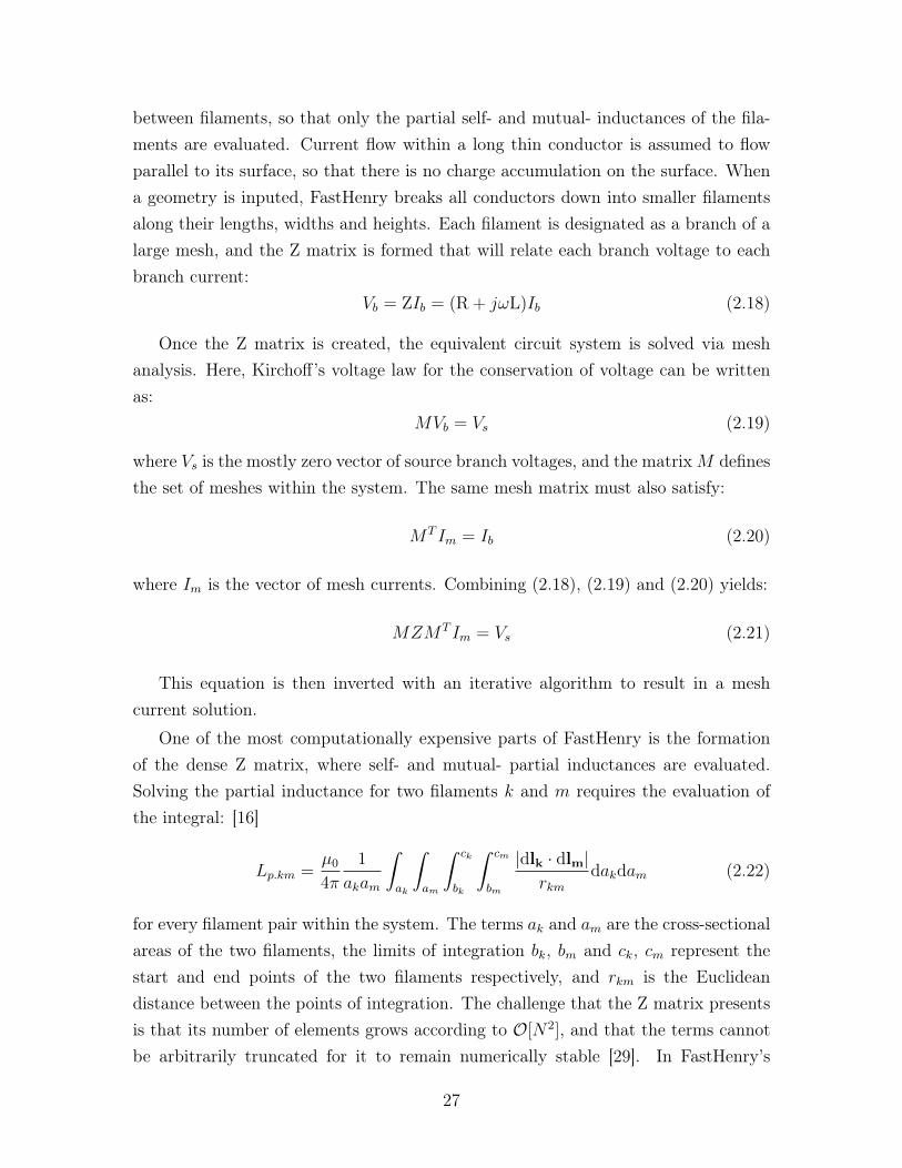
One of the most computationally expensive parts of FastHenry is the formationof the dense Z matrix, where self- and mutual- partial inductances are evaluated.Solving the partial inductance for two filaments k and m requires the evaluation ofthe integral: [16]

Lp.km =µ0

4π

1

akam

ˆak

ˆam

ˆ ck

bk

ˆ cm

bm

|dlk · dlm|rkm

dakdam (2.22)

for every filament pair within the system. The terms ak and am are the cross-sectionalareas of the two filaments, the limits of integration bk, bm and ck, cm represent thestart and end points of the two filaments respectively, and rkm is the Euclideandistance between the points of integration. The challenge that the Z matrix presentsis that its number of elements grows according to O[N2], and that the terms cannotbe arbitrarily truncated for it to remain numerically stable [29]. In FastHenry’s

27

implementation, these challenges are overcome in two ways:

• For close-by interactions, FastHenry is programmed with a plethora of closed-form analytical solutions to (2.22) from [30], [31], [32] and [16]. These solutionsavoid the need for numerical integration to be used.

• For far-away interactions, FastHenry uses the Fast Multipole Method (FMM)to compress many far-away filaments and to solve them together directly aspoint sources. The FMM reduces the order of the problem to O[N ].

These efficient techniques for obtaining the L matrix, along with clever precondition-ing of the iterative solver, are the secrets to FastHenry’s speed. Note that both ofthese techniques inherently require the Green’s function for magnetic interactions tobe that of the free-space solution to Laplace’s equation. This hard requirement onthe form of the Green’s function limits FastHenry’s usefulness in applications whereconductive, magnetic materials are used.

28

Chapter 3

The PEEC Planar Induction HeatingField Model

The accurate prediction of electromagnetic fields is crucial for the eddy current anal-ysis of induction heating. Over the past thirty years, a wealth of literature has beenbuilt around modeling the electromagnetic fields of eddy current processes using nu-merical simulation techniques. Today, there are several commercial software packagesthat can accurately treat complex eddy current physics coupled with non-linear ma-terial properties, thermal processes and mechanical deformations [15]. However, forthe purposes of computational design and optimization, the speed of the field solveris also important. In literature, order reduction and computational acceleration istypically achieved either through enforcing rotational symmetry [14, 33], or throughenforcing the so called “Manhattan symmetry”, where all heights, widths and lengthsare either parallel or perpendicular to each other [34, 35, 36].

In this chapter, we present a fast, fully three-dimensional electromagnetic fieldsolver based on the Partial Element Equivalent Circuit method (PEEC) that analyzesnon-symmetrical conductor structures placed on top, or sandwiched within infinite-extent, multilayered media. This model encapsulates a large collection of problemsincluding induction cooking [1], planar monolithic inductors and transformers [24, 34,37], microelectronic power and ground planes [35] and non-destructive eddy testingsystems [38].

The computational advantage gained by our method comes from its minimizationof volumetric meshing. As an integral formulation of Maxwell’s equations, PEECrequires only the meshing of conductive domains where current flow is expected [16],rather than over the entire system domain as in the case for domain formulationtechniques such as the finite element method (FEM) and the finite difference method

29

(FDM). However in traditional PEEC method solvers like FastHenry [28], much ofthis advantage is eroded away in the presence of a large conductive domain, such asa ground plane or conductive substrate in the case of microelectronics, or a heatedload in the case of induction heating. The traditional PEEC formulation requires theentire conductive volume to be meshed in order to account for the internally varyingcurrent flows [28]. This process dramatically increases the size of the problem andreduces the computational speed of the PEEC method.

Other integral formulations such as the boundary element method (BEM), bound-ary integral method (BIM) and the boundary integral equation method (BEIM) havebeen successfully used to replace the volumetric mesh over the conductive domainwith a surface mesh over its boundary [39, 40, 41, 42]. This is particularly efficientwhen the skin depth is negligible relative to the dimensions of the conductive domain,and the induced current is zero throughout most of the volume [27]. However on aper element basis, the formation of boundary mesh elements is more computationallyexpensive, because each element tends to be tightly coupled with all other elementsin the system.

In the method presented in this chapter, the PEEC method is modified to avoidthe explicit treatment of the conductive domains. With the assumption that theconductive domain can be approximated as an infinite-extent and uniform thicknessplane, the multilayer Green’s function can be derived to implicitly capture the effectsof the eddy currents induced within it. The multilayered Green’s function is thenembedded into the PEEC framework, and the volumetric meshing of the conduc-tive domain is avoided altogether. In previous multilayer Green’s function / PEECapproaches [37, 35], the convolution integral is resolved using the two-dimensionalFFT, restricting the conductors to cartesian Manhattan symmetry. In the followingwork, singularity-subtraction quadrature rules are used to expand the method to allthree-dimensional conductor arrangements.

3.1 The Multilayer Green’s Function Approach to

Eddy Currents

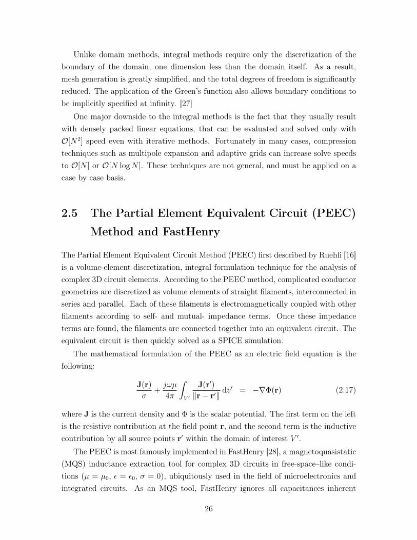
Magnetoquasistatic (MQS) systems with eddy currents are governed by the diffusionHelmholtz equation:

(∇2 − jωµσ)A = −µJsrc (3.1)

30

Here, A is the magnetic potential vector and Jsrc is the current density of the exci-tation currents. If linearity and isotropism are assumed, (3.1) can be rewritten as aconvolution integral equation:

A(r) =

ˆV ′G(r, r′) · J(r′) dv′ (3.2)

where r = (x, y, z) is the point of field evaluation, r′ = (x′, y′, z′) is one point sourceof magnetic fields, and the region of integration V ′ is the excitation currents withinthe system. Each component of the kernel of integration Gx,y,z(r, r

′) is the solutionto the magnetic diffusion Helmholtz equation for a point current source x, y, or zdirection:

(∇2 − jωµσ)Gx,y,z(r, r′) = −δ(x− x′)δ(y − y′)δ(z − z′) x, y, z (3.3)

If (3.3) is solved respecting all boundary conditions between different domains inthe z direction, the resultant solution–commonly known as the multilayer Green’sfunction–would implicitly capture the contributions of the induced eddy currents tothe magnetic fields within the system.

The multilayered Green’s function can be embedded into the PEEC formulation[16] as an electric field integral equation:

J(r)

σ+ jω

ˆV ′G(r, r′) · J(r′) dv′ = −∇Φ(r) (3.4)

where V ′ excludes the conductive layers above and below the excitation conductors.Using (3.4) with the MQS current conservation law:

∇ · J = 0 (3.5)

the excitation current density J and scalar potential Φ can be computed. With theexcitation current density J known, all fields within the system can be reconstructedusing the superposition integral (3.2).

Unfortunately, it can often be difficult to efficiently evaluate the integral in (3.4).The integration must be performed over at least three dimensions–a particularly dif-ficult task for most numerical integration techniques. Moreover, the Green’s functioncontains a singularity at r = r′, and this singularity causes the function to be numer-ically ill-conditioned when r− r′ is small.

In this chapter, both of these issues are tackled through the use of the singularity

31

subtraction technique. As discussed above, G(r, r′) is the solution to the diffusionHelmholtz equation (3.1) for the magnetic potential vector A at the field point r fora point current source at r′. Due to the superposition of fields, G(r, r′) contains botha free-space contribution from the current source itself at r′, as well as the responseof the eddy currents and magnetic domains spread throughout the entire system. Forthis reason, we can write:

G(r, r′) = Gfree(r, r′) +Gsys(r, r

′)

=µ0(xx+ yy + zz)

4π‖r− r′‖+Gsys(r, r

′) (3.6)

It is clear from (3.6) that the singularity within G originates through Gfree. Oncethe singularity is removed, the remainder Gsys is smoother and easier to integrate.Within this thesis, Gsys is denoted as the modified Green’s function.

Rewriting (3.4) with the modified Green’s function explicitly isolated:

J(r)

σ+jωµ

4π

ˆV ′

J(r′)

‖r− r′‖dv′ + jω

ˆV ′Gsys(r, r

′) · J(r′) dv′ = −∇Φ(r) (3.7)

The first two terms of the left hand side and the right hand side correspond exactlywith the traditional PEEC formulation as described by Ruehli [16], and they can beefficiently and accurately computed with existing closed-form expressions [30, 31, 32]as implemented in solvers like FastHenry [28]. The modified Green’s function termcorresponds to the eddy and magnetic domain responses of the system, and must benumerically integrated using quadrature rules. This is a considerably easier task thanbefore with the singularity removed.

The full method within this chapter can be described as a series of steps withinthe PEEC framework. One significant difference is the introduction of an initial char-acterization stage, where the modified Green’s function is computed and tabulated.This step only needs to be performed once for each layered design:

1. Derivation of the modified Green’s function. The analytical solutions forthe dyadic multilayered Green’s function are derived by hand for a specifiednumber of layers above and below the coil. The free-space Green’s functionis isolated and removed during the derivation stage, leaving an analytical ex-pression for the modified Green’s function. The mathematics of this step isdescribed in detail in Section 3.2. Here, all of the Green’s function are ex-pressed as Hankel transform integrals, and Section 3.2.3 discusses how they can

32

be quickly evaluated with numerical Hankel transform techniques.

2. Tabulation. The modified Green’s function is evaluated and tabulated sothat fast look-up table techniques can be used. Due to the inherent rotationalsymmetry, the system Green’s function is only dependent upon a fixed collectionof variables, serving as the axes of this table. These variables are the radialdistance of the source and field points r−r′ =

√(x− x′)2 + (y − y′)2, the sums

and differences of their heights (z + z′), (z − z′) and the frequency f .

Once the layers are characterized, each subsequent induction coil design can be eval-uated with the following steps :

1. Input. A list of N filaments is inputed and numbered from 1 to N .

2. Formulation of the free-space Z matrix. For each filament pair, the mutualimpedance between them in free-space conditions is calculated using closed-formsolutions and stored as a cell within an N ×N matrix denoted as the Z matrix.

3. Calculation of the system contribution. For each cell in the Z matrix, themutual impedance contribution of the system is calculated by convolving themodified Green’s function via multidimensional sparse grid quadrature. Thequadrature equations are (3.68)-(3.70), and (3.73)-(3.75); details on their im-plementation can be found in Section 3.3. This is the most computationallyexpensive step of the algorithm.

4. Solve for system currents. A known voltage excitation is applied to theterminals of the induction coil. The Z matrix, corrected with the system con-tribution, is used with the FastHenry implementation of the PEEC method.Mesh analysis is performed, and the linear equations are solved with GMRESto result in a current value for each filament. For details on how the Z matrixis used to solve for system currents, see the original FastHenry implementation[28]. The impedance of the coil is taken to be the ratio between the appliedvoltage and the terminal current solved through this step.

5. Solve for fields. With all the currents known, the fields are solved at areas ofinterest. Firstly, the free-space contribution is solved at each field point usingclosed-form solutions. Then, quadrature rules are used to solve for the systemcontributions, by numerically convolving the modified Green’s function withthe known current densities. The fields are used to calculate the induction heatprofile according to Section 3.4.

33

Note that step 4 can be avoided if the conductors are only discretized along theirlengths, and not over their cross-sectional areas. As all the filaments are connectedin series, the current flowing through all the filaments must be identical. The partialimpedances (i.e. each entry of the Z matrix) can be fused together into a singleequivalent circuit element by simple summation, and this value is indeed the terminalimpedance of the coil.

3.2 Derivation of the Multilayer Green’s functions

The multilayer Green’s functions for two geometries are presented in this section.The first is the semi-infinite half-space, which has been extensively studied boththeoretically and experimentally from the early days of eddy current analysis. Thesemi-infinite geometry is known to be an accurate model of eddy currents when thepenetration depth of the electromagnetic fields is small relative to the depth of thesurface. These are sufficient approximations for a wide range of applications in do-mestic induction heating [1].

The second geometry considered is the general multilayered problem, where N+1

distinct layers of homogenous magnetic permeability and conductivity are stackedon top of one another in the z direction. The excitation currents can either beplaced above the entire stack or sandwiched in between specific layers. This generalarrangement embodies the cases where the depth of penetration through at least oneof the layers is comparable to the thickness of that layer, and that the heated surfacecan no longer be considered to be semi-infinite in its depth. For domestic inductionheating, the multilayered problem is applicable when a non-ferromagnetic material(e.g. aluminum or copper) is heated.

In both cases, it is important to note that the multilayered Green’s function isdyadic, and that it is expressed as a tensor field rather than a vector or a scalar field.This reflects the fact that for each component of the current density vector J, cross-coupling can occur, causing the resultant A field to have components in all threedimensions. The dyadic Green’s function is often written using the tensor notation:

G =[Gx Gy Gz

]=

Gxx Gxy Gxz

Gyx Gyy Gyz

Gzx Gzy Gzz

(3.8)

such that Gjk is the Green’s function contribution of a current in the k direction to

34

the magnetic potential vector in the j direction. The Green’s function convolutionintegral is then rewritten as a dot product equation in the following form:

A(x, y, z) =

ˆC

I(x, y, z)G(x, y, z) · ds (3.9)

where ds is the line integral vector, C is the contour of the conductor and I(x, y, z)

is the magnitude of the current at that point.

3.2.1 The Dyadic Green’s Function for the Semi-Infinite Half-

Space

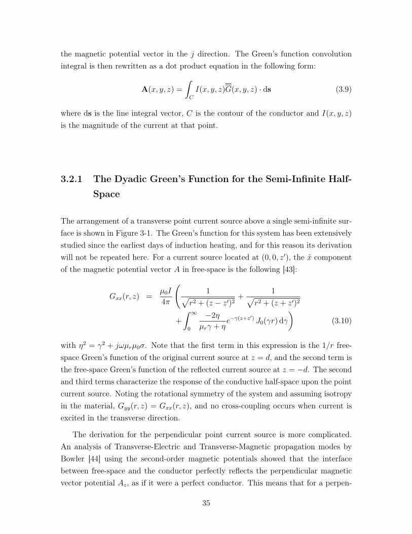
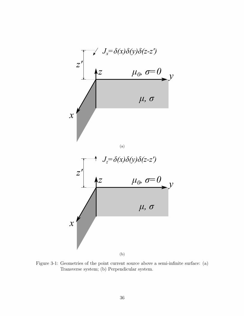
The arrangement of a transverse point current source above a single semi-infinite sur-face is shown in Figure 3-1. The Green’s function for this system has been extensivelystudied since the earliest days of induction heating, and for this reason its derivationwill not be repeated here. For a current source located at (0, 0, z′), the x componentof the magnetic potential vector A in free-space is the following [43]:

Gxx(r, z) =µ0I

4π

(1√

r2 + (z − z′)2+

1√r2 + (z + z′)2

+

ˆ ∞0

−2η

µrγ + ηe−γ(z+z′) J0(γr) dγ

)(3.10)

with η2 = γ2 + jωµrµ0σ. Note that the first term in this expression is the 1/r free-space Green’s function of the original current source at z = d, and the second term isthe free-space Green’s function of the reflected current source at z = −d. The secondand third terms characterize the response of the conductive half-space upon the pointcurrent source. Noting the rotational symmetry of the system and assuming isotropyin the material, Gyy(r, z) = Gxx(r, z), and no cross-coupling occurs when current isexcited in the transverse direction.

The derivation for the perpendicular point current source is more complicated.An analysis of Transverse-Electric and Transverse-Magnetic propagation modes byBowler [44] using the second-order magnetic potentials showed that the interfacebetween free-space and the conductor perfectly reflects the perpendicular magneticvector potential Az, as if it were a perfect conductor. This means that for a perpen-

35

μ, σ

μ0, σ=0

x

yz

Jx=δ(x)δ(y)δ(z-z')

z'

(a)

μ, σ

μ0, σ=0

x

yz

Jz=δ(x)δ(y)δ(z-z')

z'

(b)

Figure 3-1: Geometries of the point current source above a semi-infinite surface: (a)Transverse system; (b) Perpendicular system.

36

dicular source at (0, 0, z′):

Gzz(r, z) =µ0I

4π

[1√

r2 + (z − z′)2+

1√r2 + (z + z′)2

](3.11)

However, in the perpendicular mode of excitation, some energy is cross-coupledto the radial direction. Juillard et al. derived this Green’s function to be [43]:

Grz(r, z) =µrµ0I

2π

ˆ ∞0

γ

µrγ + ηe−γ(z+z′) J1(γr) dγ (3.12)

The Cartesian Green’s functions Gxz(r, z) and Gyz(r, z) can be retrieved by thesubstitution r = (x − x′)/‖r − r′‖x + (y − y′)/‖r − r′‖y. Thus the overall Green’sfunction tensor can be written as:

G(r, r′) =

Gxx(r, r

′) 0 0

0 Gxx(r, r′) 0

|x−x′|√(x−x′)2+(y−y′)2

Grz(r, r′) |y−y′|√

(x−x′)2+(y−y′)2Grz(r, r

′) Gzz(r, r′)

(3.13)

It is important to note that for each Green’s function, the quasistatic condition∇·E = −jω∇·A = 0 does not hold, because the current filament does not constitutea closed loop. Thus for these equations to have any physical significance, ∇ ·A = 0

must be explicitly enforced once the loop is closed. First, consider a closed loopconvolution integral along some contour with the dyadic Green’s function.

A(r) =

˛G(r, r′) · ds =

˛G(r, r′) · t dl (3.14)

A(r) denotes the magnetic vector potential of the final closed loop measured at thefield point r. The integration is performed with ds along the along the r′ = (x′, y′, z′)

source point coordinates. The tensor dot product can be broken up into its threecomponents:

A =

˛Gxxx(x · t) dl +

˛Gxxy(y · t) dl +

˛Gz(z · t) dl (3.15)

Note that only Gxx and Gyy of the vectors Gx and Gy are non-zero, because cross-coupling does not occur in the transverse direction. The divergence of this expression

37

is:

∇ ·A =

˛δ

δxGxx(x · t) dl +

˛δ

δyGxxy(y · t) dl

+

˛(∇ ·Gz)(z · t) dl (3.16)

To ensure that the closed loop divergence is zero, the line integral on the righthand side of (3.16) must evaluate to zero. By the fundamental theorem of calculus,this is guaranteed if the integrand of (3.16) can be expressed as a gradient vector fieldwith respect to the variables of integration, that is the source variables x′, y′, z′. Asit currently stands, (3.16) can be written as the line integral around the vector fieldF:

∇ ·A =

˛F · ds (3.17)

where

F =

δδxGxx

δδyGxx

∇ ·Gz

(3.18)

To show that F is a gradient field with respect to the source variables, note thatin the transverse directions, Gxx has a dependence on (r − r′). Because of this,

δ

δxGxx = − δ

δx′Gxx,

δ

δyGxx = − δ

δy′Gxx (3.19)

and

F =

−δδx′Gxx

− δδy′Gxx

∇ ·Gz

(3.20)

If the following gauge condition is imposed:

∇ ·Gz = − δ

δz′Gxx (3.21)

thenF = −∇′Gxx (3.22)

where ∇′ is the del operator with respect to the source variables x′, y′, z′. SinceGxx is smooth and continuous due to the boundary conditions imposed on it, F is aconservative gradient field, and the closed loop line integral around F by ds traversingas the vector r′ must sum to zero. Thus as it is shown, ∇ ·A = 0 is guaranteed if the

38

gauge condition in (3.21) is satisfied. One can verify that this is indeed the case for(3.11) and (3.12).

3.2.2 The Dyadic Green’s function Multiple-Layered Config-

uration

Preliminary work on multiple-layered conductors were first conducted in the earliestdays of eddy current analysis by Dodds and Deeds in 1968, with their derivation ofthe equations for the two-layered conductor [6]. A particularly interesting geometryfor the purpose of induction heating is known as the “sandwich” configuration, wherethe coil is placed between two conductive materials. Derivations for a circular coilplaced within specific sandwich arrangements were presented by Hurley et al. [25].These expressions were adapted by Acero et al. for the induction heating application[45], and developed into generalized expressions for all multilayered configurations[12].

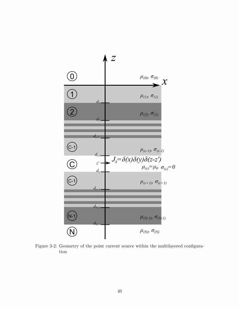
Transverse Component

Consider the multilayered system in Figure 3-2. The system is arranged with each ofthe multiple layers stretched infinitely along the x and y axes, with depth in the zdirection. For mathematical convenience, the boundary for the first, top layer startsat z = 0, and each subsequent layer boundary is located at z = di where di relatesto the deepest edge of layer i. Noting the rotational symmetry, the Hankel transformcan be taken along the radial dimension:

Ai(r, z) =

ˆ ∞0

A∗i (k, z)kJ0(kr) dk (3.23)

The transformed variables A∗i can be placed into the diffusion equation to resultin a general expression for A∗i :

A∗i =

Bi sinh(ηi(z − di)) + Ci cosh(ηi(z +−di)) i ∈ 1 . . . N − 1

C0e−η0z i = 0

CNeηN (z+dN ) i = N

(3.24)

where η2i = k2 + jωµiσi. The magnetic field in the y direction Hy has the following

39

1

0

2

C-1

C

C-1

N-1

N

x

z

μ(0), σ(0)

μ(1), σ(1)

μ(2), σ(2)

μ(c-1), σ(c-1)

μ(c)=μ0 σ(c)=0

μ(c+1), σ(c+1)

μ(N-1), σ(N-1)

μ(N), σ(N)

d1

d2

dc-2

dc-1

dc

dc+1

dN-1

dN-2

Jx=δ(x)δ(y)δ(z-z')z'

Figure 3-2: Geometry of the point current source within the multilayered configura-tion

40

values:

H∗i =

Biλi cosh(ηi(z − di)) + Ciλi sinh(ηi(z − di)) i ∈ 1 . . . N − 1

−C0λ0e−η0z i = 0

CNλNeηN (z+dN ) i = N

(3.25)

where λi = ηi/µi. The middle layers will require boundary matching. At the bottomof each middle layer (i ∈ 1 . . . N − 1) where z = di:

A∗i = Ci, H∗i = Biλi (3.26)

At the top of each middle layer where z = di−1:

A∗i = Bi sinh(ηiti) + Ci cosh(ηiti) (3.27)

H∗i = Biλi cosh(ηiti) + Ciλi sinh(ηiti) (3.28)

where ti is the depth of layer i: ti = di − di−1. Let both A∗i and H∗i be continuousalong each middle boundary:[

λi+1

λicosh(ηi+1ti+1) λi+1

λisinh(ηi+1ti+1)

sinh(ηi+1ti+1) cosh(ηi+1ti+1)

](Bi+1

Ci+1

)=

(Bi

Ci

)(3.29)

Let us denote this matrix as M i+1. Note that the matrix is easily inverted:

[λiλi+1

cosh(ηi+1ti+1) − sinh(ηi+1ti+1)

− λiλi+1

sinh(ηi+1ti+1) cosh(ηi+1ti+1)

](Bi

Ci

)=

(Bi+1

Ci+1

)(3.30)

Now, consider a transverse current filament of current I in layer c, at the depth ofz = z′. Furthermore, let this layer be free-space. This filament changes the boundaryconditions at the top and bottom of layer c to be respectively:

A∗c(z = dc−1) = Bc sinh(ktc) + Cc cosh(ktc) +µ0I

4πke−k(dc−1−z′) (3.31)

H∗c (z = dc−1) = Bck

µ0

cosh(ktc) + Cck

µ0

sinh(ktc)−I

4πe−k(dc−1−z′) (3.32)

A∗c(z = dc) = Cc +µ0I

4πke−k(dc+z′) (3.33)

H∗c (z = dc) = Bck

µ0

+I

4πe−k(dc+z′) (3.34)

41

The boundary conditions for the layers above and below the coil layer can bewritten as two matrix equations:

M c+1

(Bc+1

Cc+1

)=

(Bc

Cc

)+

(1

1

)µ0I

4πke−k(dc+z′) (3.35)

M c

(Bc

Cc

)+

(− kµ0λc−1

1

)µ0I

4πke−k(dc−1−z′) =

(Bc−1

Cc−1

)(3.36)

At the boundary of the uppermost layer, where z = 0:

M1

(B1

C1

)=

[λ1λ0

cosh(η1t1) λ1λ0

sinh(η1t1)

sinh(η1t1) cosh(η1t1)

](B1

C1

)=

(−1

1

)C0 (3.37)

Let Φ = λ1−λ0λ1+λ0

, eliminating this into one row and simplifying the hyperbolictrigonometry:

[1 2Φ

e2η1t1+Φ

]( B1

C1

)= 0 (3.38)

At the boundary of the lowermost layer, where z = dN−1:

[λN−1

λN−1

]( BN−1

CN−1

)= 0 (3.39)

Thus, the five matrix equations of (3.35), (3.36), (3.38) and (3.39) can be writtento match all the boundary conditions. Simultaneously solving the matrices as onelinear equation system:

C 0 0 0 0 0

−I2 M2 0 0 0

0 0. . . 0

−I2 M c

−I2 M c+1

0. . . 0 0

0 0 0 −I2 MN−2

0 0 0 0 0 D

Γ1

Γ2

...Γc−1

Γc

Γc+1

...ΓN−2

ΓN−1

=

0

0...0

Fc

Fc+1

...0

0

42

with M i defined according to (3.29), and:

Γi =

(Bi

Ci

)(3.40)

C =[

1 2Φe2η1t1+Φ

](3.41)

D =[

λN−1

λN−1

](3.42)

Fc =

(k

µ0λc−1

−1

)µ0I

4πke−k(dc−1−z′) (3.43)

Fc+1 =

(1

1

)µ0I

4πke−k(dc+z′) (3.44)

A number of matrix inversion technique can then be applied to solve for all un-known coefficients in the system. Once Bc and Cc are calculated from the matrixequation system, the Green’s function in the coil layer c can be written as:

Gxx.c(r, z) = Ac(r, z) =µ0I

4π

1√r2 + (z − z′)2

+

ˆ ∞0

[Bc sinh(k(z − dc))

+Cc cosh(k(z − dc))] kJ0(kr) dk (3.45)

In practice, both Bc and Cc are dependent upon k, and the matrix equation canonly be numerically solved for a single k value. In the interest of computationalspeed, it is necessary to tabulate the Green’s function with respect to r, z and z′,rather than to calculate it on-the-fly. Note that while (3.45) is similar in appearanceto previous works [12], its advantage is that the 1/r free-space Green’s function isexplicitly isolated during the formulation stage.

Perpendicular Component

The derivation for the perpendicular component of the multilayer Green’s functionextends the half-space derivation in Section 3.2.1. Here, the H field generated bya perpendicular current filament in the multilayered configuration exists only in theφ direction, due to the cylindrical symmetry of the system and the orthogonalityimposed by the definition of the magnetic potential vector and the diffusion equation.Because of this, A exists only in the r and z directions, and does not have any valueor any dependence along φ.

First, as shown in the case for the semi-infinite half-plane by Bowler [44], Az = 0

is enforced within all the regions except the source region. This means for a coil

43

placed in layer c at a depth of z′:

A∗z.i =

µ0I4πke−k|z−z

′| +Dc sinh(k(z − dc)) + Fc cosh(k(z − dc)) i = c

0 i 6= c(3.46)

The radial component is treated in a similar way to how it was treated in thetransverse case, but is now transformed with the first-order Hankel transform:

A∗ri =

Bi sinh(ηi(z − di)) + Ci cosh(ηi(z − di)) i ∈ 1 . . . N − 1

C0e−η0z i = 0

CNeηN (z+dN ) i = N

(3.47)

The radial magnetic field Hr = 1µ( δδrAz− δ

δzAr). Noting that δ

δrJ0(kr) = −kJ1(kr)

and keeping the same definition of λi from before:

H∗ri =

−Biλi cosh(ηi(z − di))− Ciλi sinh(ηi(z − di)) i ∈ 1 . . . N − 1, i 6= c

C0λ0e−η0z i = 0

−CNλNeηN (z+dN ) i = N

(3.48)

It is clear from these sets of equations that the boundary matching matrix M i+1

would be the same as in the transverse current case. This makes sense physicallybecause only the transverse A and H fields are matched in either cases. However, Hr

is more complicated than the transverse case at the layer containing the coil:

H∗rc = −λc[µ0I

4πke−k|z−z

′| +Dc cosh(k(z − dc)) + Fc sinh(k(z − dc))

+Bc cosh(ηc(z − dc)) + Cc sinh(ηc(z − dc))] (3.49)

The following conditions result from (3.46) and (3.49) at the coil layer boundaries:

M c+1

(Bc+1

Cc+1

)=

(Bc

Cc

)+

(1

0

)[Dc +

µ0I

4πke−k(dc+z′)

](3.50)

44

M c

(Bc

Cc

)+

(k

µ0λc−1

0

)[Dc cosh(ktc))

+Fc sinh(ktc)) +µ0I

4πke−k(dc−1−z′)

]=

(Bc−1

Cc−1

)(3.51)

The gauge condition of (3.21) is enforced as the final boundary condition. This ismost easily done with one of the layers without the coil, for example layers 0 and N:

C0 = −1

k

δ

δz′Cxx.0 (3.52)

CN = −1

k

δ

δz′Cxx.N (3.53)

where Cxx.0 is the coefficient for the Green’s function of layer 0 in the transversecase, also named C0 in (3.24). These equations combine to form a second set of matrixequations:

C 0 0 0 0 0

−I2 M2 0 0 0

0 0. . . 0

−I2 M c

−I2 M c+1

0. . . 0 0

0 0 0 −I2 MN−2

0 0 0 0 0 D

Γ1

Γ2

...Γc−1

Γc

Γc+1

...ΓN−2

ΓN−1

=

0

0...0

Fc

Fc+1

...0

0

with M i defined according to (3.29), and Γi, C and D as before in (3.40)-(3.42). Thenew right hand side is:

Fc =

(−k

µ0λc−1

0

)[Dc cosh(ktc)) + Fc sinh(ktc)) +

µ0I

4πke−k(dc−1−z′)

](3.54)

Fc+1 =

(1

0

)[µ0I

4πke−k(dc+z′) +Dc

](3.55)

and Dc, Fc are solved by the substitutions in (3.52) and (3.53). The final Green’s

45

functions are:

Gzz.c(r, z) =µ0I

4π

1√r2 + (z − z′)2

+

ˆ ∞0

[Dc sinh(k(z − dc))

+Fc cosh(k(z − dc))] kJ0(kr) dk (3.56)

and

Grz.c(r, z) =

ˆ ∞0

[Bc sinh(k(z − dc)) + Cc cosh(k(z − dc))] kJ1(kr) dk (3.57)

3.2.3 Application of Numerical Hankel Transforms

Due to the inherent radial symmetry for the planar-symmetric geometry, all of theGreen’s functions above can be expressed as Hankel transform integrals, where theHankel transform is defined to be

F (k) = Hν [f(r)] =

ˆ ∞0

f(r) Jν(kr)r dr (3.58)

f(r) = H−1ν [F (k)] =

ˆ ∞0

F (k) Jν(kr)k dk (3.59)

Here, Jν is the order ν Bessel function of the first kind. This integral is challenging formost numerical quadrature algorithms, due to the oscillating kernel of the integraland the unbounded integration domain. Fortunately, there exist a variety of algo-rithms designed to numerically evaluate the Hankel transform integral with a singletransformation operation for a set of r values. The use of these specialized algorithmsgreatly accelerates the computation of the Green’s functions.

Two important algorithms considered here are the Quasi-Fast Hankel Transform(QFHT) by Siegman [46] and the Quasi-Discrete Hankel Transform (QDHT) byGuizar-Sicairos and Gutierrez-Vega [47]. While other algorithms exist, such as theHigh-accuracy Fast Hankel Transform (HAFHT) [48] and various back projection andslice projection methods [49], these two algorithms stand out as the benchmark usedin literature due to their high performance and ease of implementation. Both wereincluded as components of the model, although empirically the QDHT was found tobe better performing.

Quasi-Fast Hankel Transform

The Quasi-Fast Hankel transform (QFHT) [46] characterizes an entire family of im-portant algorithms where the variables r and k from (3.58),(3.59) are discretely sam-

46

pled according to an exponential pattern:

rm = roeαm, kn = koe

αn (3.60)

Here, α is a common scaling factor shared between the two variables. By substi-tuting the exponentially sampled discrete rm and kn into the Hankel transform anddiscretizing, the Hankel transform is simplified to a discrete cross-correlation relation.The cross-correlation can then be rapidly evaluated using the fast Fourier transformalgorithm.

The QFHT and other exponentially sampled algorithms are widely praised fortheir O[N logN ] speed and their efficient use of memory [49]. Unfortunately, the useof exponential sampling is often inconvenient, and the interpolation, quadrature orresampling scheme required to rectify this adds an additional layer of computationtime and loss of accuracy. Moreover, it is often difficult to control the error size ofthe algorithm, because it is influenced by the arbitrary parameters ro, ko and α inaddition to the number of terms used to evaluate the transform.

Quasi-Discrete Hankel Transform

The Quasi-Discrete Hankel Transform (QDHT) is an algorithm first developed forthe zeroth order Hankel transform by Yu et al. [50], and later on extended to integerorder Hankel transforms by Guizar-Sicairos and Gutierrez-Vega [47]. The algorithmis based on using a closed-form approximation of the transform equations (3.58),(3.59) at the roots of the Bessel functions of the first kind. Addressing many issuesof the QFHT, the QDHT algorithm produces a uniformly sample output, and withits accuracy controlled only by the number of samples used. However, it is alsoconsiderably slower and more storage intensive, because the actual transformation isperformed with an O[N2] matrix multiplication.

3.3 Evaluation of the Modified Green’s Function via

Quadrature

As explained in Section 3.1, the dyadic Green’s function of a point current sourcewithin a multilayered system can be decomposed into two components: the free-space Green’s function due to the point current source itself, and the modified Green’sfunction due to the eddy currents and magnetic domains of the rest of the system.

47

While several closed form solutions to the free-space Green’s function have beenderived, the modified Green’s function must be numerically integrated to obtain theresponse of the conductive magnetic surface.

The challenge of the task lies in the need to integrate over several dimensions:the interaction between two finite-volume conductors will require integration oversix dimensions (twice for each cartesian dimension) [16]. Conventional numericalintegration algorithms are bound by the “curse of dimensionality”, because the costof such an operation grows at an exponential rate, to the point of being impracticalonce more than two or three dimensions are considered. This issue of dimensionalitywas identified as an overwhelming challenge by previous authors [37].

Fortunately, over the past two decade, several numerical integration schemes havebeen developed that can overcome the curse of dimensionality:

• Smolyak’s construction, also known in literature as the blending method, theboolean method, or the sparse grid method. In this approach, multidimensionalquadrature formulas are constructed from the tensor products of a suitable one-dimensional quadrature formula. [51]

• Lattice Methods, a simple and mathematically elegant technique, based on thegeneralizations of the rectangle rule, for integrating smooth, periodic functionsover many dimensions. Non-periodic functions can too be integrated by latticemethods when a nonlinear transformation is used before the quadrature [52].

• Monte Carlo and deterministic Monte Carlo techniques, based on probabilistictechniques [53].

• Adaptive subdivision rules, that intelligently allocates quadrature points to eachdimension according to its importance [54, 55].

Each one of these schemes is developed to be efficient for a specific set of problem,for which it can then evaluate with logarithmic growth of costs with increasing di-mensionality.

The quadrature scheme used within this thesis is a sparse grid formulation byHeiss and Winschel [56]. Compared to the other options, the sparse grid formulationis the fastest performing quadrature scheme of the options available, being a singleprocess involving only function evaluations and multiplication. However, the abilityto estimate and control the quadrature within a certain error tolerance is lost. Giventhe smoothness of the modified Green’s function with the singularity removed, thiswas deemed to be an acceptable price to pay.

48

In the version of the quadrature used, the standard Gauss-Legendre quadratureis used for the base one-dimensional quadrature scheme, and it is extended to higherdimensions using Smolyak’s combination of tensor products. The integration overa hypercube of many dimensions is then approximated as a series of weights andfunction evaluations at specific points. For example, a six-dimensional integrationover the hypercube Ω = [0, 1]6 is approximated with a six-dimensional quadraturescheme: ˆ

Ω

f(x, y, z, x′, y′, z′) d x, y, z, x′, y′, z′ ≈N∑j=0

wjf(pj) (3.61)

where wj is a series of weights and pj is a series of evaluation points. The supplementalcode library supplied by Heiss and Winschel was used to generate the weights andevaluation points.

Filament to filament interaction

The partial mutual inductance contribution can be calculated by integrating the elec-tric field generated by one filament with the remainder of the Green’s function alongthe contour of another. Using the modified multilayered dyadic Green’s function G,the field generated by filament 1 in the x direction can be expressed in tensor dotproduct form as:

Ek(r) = jωI

ˆ ck

bk

G(r, r′) · dl1

Integrating the electric field along the contour of filament 1, and dividing by thecurrent flowing through conductor 1 and jω yields the mutual inductance M :

M =

ˆ ck

bk

ˆ cm

bm

G(r, r′) · dl1 · dl2 (3.62)

M =

ˆ ck

bk

ˆ cm

bm

G(r, r′) · t1 · t2 dl1 dl1 (3.63)

The paths of integration are:

r′ = s1 + l1t1 (3.64)

r = s2 + l2t2 (3.65)

where s1 and s2 are the starting points and t1 and t2 are the unit vectors pointing

49

tangentially along the lengths of each filament. To resolve the anisotropy of the dyadicGreen’s function, let us define a new unit vector, T as the normalized projection oft1 to the transverse plane:

T =(t1 · x)x+ (t1 · y)y√

(t1 · x)2 + (t1 · y)2

(3.66)

With this, t1 can be broken down into its transverse and perpendicular compo-nents:

t1 = (t1 · T )T + (t1 · z)z (3.67)

The T component of t1 generates a field purely in the T direction. The portion ofthis field that is coupled to the second conductor is equal to (t2 · T ). Thus:

MT = (t1 · T )(t2 · T )

ˆ L1

0

ˆ L2

0

Gxx(r, r′) dl1 dl2 (3.68)

The z component of t1 generates two orthogonal fields, one in the z directionand one in the transverse radial direction r from the source point to the field point.Describing the components as interactions in three dimensions:

Mzz = (t1 · z)(t2 · z)

ˆ L1

0

ˆ L2

0

Gzz(r, r′) dl1 dl2 (3.69)

Mrz =

ˆ L1

0

ˆ L2

0

(t2 · x) |x− x′|+ (t2 · y) |y − y′|√(x− x′)2 + (y − y′)2

Grz(r, r′) dl1 dl2 (3.70)

The total mutual inductance is the sum of these orthogonal components, M =

MT +Mzz +Mrz.

Conductor to conductor interaction

The filament approximation used to derive these analytical solutions also introduceserrors, because real conductors have finite cross-sections that also contribute fieldstowards the fields of the system. This effect is well understood if the current densityis assumed to be constant throughout the conductor. The Geometric Mean Distance(GMD) method can be used to calculate correction factors to compensate for theerrors introduced by the filament approximation [31, 57]. With circular cross sections,the filament approximation is said to be accurate to about 15 parts in 1000 withoutthe need for a correction factor [31]. The constant current density assumption is

50

generally valid for a wide range of frequencies if the coil is wound with litz wires.As the volume of the filaments increases in proportion to their relative distances,

the cross-sectional areas can no longer be ignored. In this case, the average mutualimpedance over the cross-sectional areas of the conductors can be taken to extendthe zero-volume results to the finite-volume conductor. For this to be applicable, twoassumptions must hold: (1) current flows only in the direction along the length of theconductor; (2) current density is uniform within the conductor.

To perform this averaging over the cross-sectional areas of both conductors, con-sider extending the definition of r and r′ from (3.64) and (3.65) with two additionalcomponents in orthogonal directions:

r′ = s1 + l1t1 + w1w1 + h1h1 (3.71)

r = s2 + l2t2 + w2w2 + h2h2 (3.72)

where wj and hj are the unit vectors pointing along the widths and heights of eachfilament. Extending (3.68), the transverse component can now be written as:

MT =(t1 · T )(t2 · T )

W1W2H1H2

ˆ L1

0

ˆ L2

0

ˆ W1

0

ˆ W2

0

ˆ H1

0

ˆ H2

0

Gxx(r, r′) d l1, l2, w1, w2, h1, h2

(3.73)Similarly averaging over the cross-sectional areas in (3.69) and (3.70):

Mzz =(t1 · z)(t2 · z)

W1W2H1H2

ˆ L1

0

ˆ L2

0

ˆ W1

0

ˆ W2

0

ˆ H1

0

ˆ H2

0

Gzz(r, r′)

d l1, l2, w1, w2, h1, h2 (3.74)

Mrz =1

W1W2H1H2

ˆ L1

0

ˆ L2

0

ˆ W1

0

ˆ W2

0

ˆ H1

0

ˆ H2

0

(t2 · x) |x− x′|+ (t2 · y) |y − y′|√(x− x′)2 + (y − y′)2

·Grz(r, r′) d l1, l2, w1, w2, h1, h2 (3.75)

As before, the total mutual inductance is the sum of these orthogonal components,M = MT +Mzz +Mrz.

3.4 Eddy Current Loss Profile

In order to determine the heating profile and temperature profile of the heated load,the field model must also evaluate the eddy current loss profile within the conductive,magnetic media. As an integral formulation method, the PEEC model only solves forthe currents flowing through the filaments. In order to obtain the field strength within

51

the domain, the Green’s function must be convolved with the evaluated boundaryvalues at specific observation points.

3.4.1 Theoretical Basis

By the Poynting theorem, the complex power crossing the z = 0 interface from thez > 0 region can be described by the time-averaged Poynting’s vector in the z directionalong this plane:

S =

ˆsurface

1

2(E×H∗) · (−z) da (3.76)

where the asterisk here denotes the complex conjugate. If the bounds of the integra-tion are extended to infinity then the fields on the side of the box are reduced to zero.The only non-zero integration surface is z = 0. Applying the divergence theorem, theidentity ∇ · (E ×H∗) = (∇× E) ·H∗ − (∇×H∗) · E and the standard constitutiverelations:

S =jω

2µ

ˆV

‖B‖2 dV +σ

2

ˆV

‖E‖2 dV (3.77)

where the volume V corresponds to the conductive z < 0 region. The first term herecorresponds to the magnetic storage of energy, and the second term corresponds toeddy losses in the load. Due to the MQS approximation in place, the electric fieldstores no energy.

Most induction heating loads have magnetic permeabilities of µr 1. Becauseof this, their refractive indices are very high and the internal electromagnetic waveswithin them are approximately plane waves propagating in the −z direction. Underthese conditions, transverse power flow is negligible to perpendicular power flow, and:

1

2(E×H∗) · (−z) =

jω

2µ

ˆ −∞0

‖B‖2 dz +σ

2

ˆ −∞0

‖E‖2 dz (3.78)

The absence of tangential power flow beneath the interaction surface is an impor-tant assumption for our formulation to hold. Consider the scalar field P , defined asthe real component of the Poynting vector:

P = Re

1

2(E×H∗) · (−z)

(3.79)

such that˜P da = Re S. If tangential power flow is negligible, then P can be

used directly as the heating profile over the surface of the load.

52

The use of the Poynting vector is well-established in induction heating for thesemi-infinite half-plane configuration discussed previously in Section 3.2.1. With ahomogenous and isotropic eddy current media, it can be shown that all fields decayat a rate of the skin depth δ =

√2/(ωµσ). With this, P becomes the classic surface

resistance relation:

P =1

2σδ

(‖Hx(z = 0)‖2 + ‖Hy(z = 0)‖2

)For generality however, it is necessary to obtain a relation for P that will work

on heated loads conductors of all thickness and layer compositions. Noting that Azis approximately zero for a mostly planar coil system, (3.79) simplifies to:

P = − ω

2µIm

Ax

(δA∗xδz

)+ Ay

(δA∗yδz

)(3.80)

The values of A, and δA/δz can be calculated by convolving the Green’s functionalong the source currents, as discussed in Section 3.4.2.

An aside observation is that if conductive materials are only placed in the regionof x < 0, then heat flow is only in the direction of −z. The total integral of P overthe entire interface plane z = 0 should give the total eddy current power loss withinthe material. This is one method to obtain the reflected resistance of the load to theterminals of the coil, i.e.

∆R =2

I2

¨ +∞

−∞P (x, y) dx dy (3.81)

where I is the current driven into the coil, and ∆R is the terminal reflected resistanceof the load, from the four-element model of Figure 2-2.

3.4.2 Implementation Details

To calculate the heating profile of an induction coil, the result shown in (3.80) canbe applied by evaluating the A field along the interface surface. First, to obtainthe A field at relevant points, N observational points are placed in a grid formationalong the z = 0 plane, and N points at a small distance above, z = δ = 10−5m.This results in 2N observation points: Oj = (Ox.j, Oy.j, Oz.j), j ∈ 1 · · · 2N . The goalhere is to convolve the dyadic Green’s function over every filament, with each of theobservational points fixed as the field points.

First, for a system ofM filaments, we define the vector function φj(r), k ∈ 1 · · ·M

53

with

φj(r) =

tj within the filament j

0 outside the filament j

where tj is the unit vector tangential along the length of the filament. With this, thematrix L can be formed with each element at the j-th row and k-th column as

Ljk =

ˆS′G(Oj, r’) · φk(r′) dS ′ (3.82)

Effectively, each entry of L is the Green’s function, convolved over the support ofthe filament basis function φk(r) for observational point Oj. If the current of eachfilament Ij is combined into a column vector I, then the matrix equation can bewritten:

LI = A (3.83)

Each row of A is the A field measured at each of the 2N observational points. Toobtain a difference estimation of the gradient δA/δz, take the difference between thefirst N field points measured at z = 0 and the second N points measured at z = δ,and divide the result by δ. Substituting the evaluated Ax, Ay, δAx/δz and δAy/δz

values for each observational point Oj into (3.80), the value of the eddy current losspower flux is obtained at each observation point.

3.5 Comparison to Previous Analytical Models

Early seminal work in MQS partial differential equations have yielded a number ofanalytical solutions of the induction heating problem for the circular coil. In thissection, we will compare the simulated predictions based on our method with existinganalytical solutions.

The mutual impedance between two zero-volume circular filaments suspendedabove a semi-infinite half-plane can be written in the form of a Sommerfeld integral[58, 24, 19]:

Zm = jωµ0πr1r2

ˆ ∞0

(e−k|d1−d2| +kµr − ηkµr + η

e−k(d1+d2)) J1(kr1) J1(kr2) dk (3.84)

with η2 = k2 + jωµrµ0σ. The same solution can also be obtained by some minoralgebra on the Dodds and Deeds solution [6], or by taking the associated Green’sfunction from Section 3.2.1 and convolving it along the two circular contours in the

54

Hankel domain.

When solved for a circular coil, (3.84) gives the ∆R and L0 +∆L parts of the four-element model of Figure 2-2. The series resistance of the coil R0 must be separatelyevaluated.

3.5.1 Acero et al.

Equation (3.84) was experimentally verified by Acero et al. for a 23-turn inductionheating coil placed below a ferromagnetic plate [19]. We can recover the measurementsmade by Acero by evaluating (3.84) under the same conditions described. The heatedferromagnetic plate has the following properties: µr = 130, σ = 8 × 106 S/m. Theplate is placed a distance of 4 mm above the coils. The coils are arranged as aseries of flat concentric circular filaments, with 23 turns evenly spread from 2.5 cmto 10.5 cm. Evaluating the free-space mutual impedance Sommerfeld integral gives afrequency-independent free-space inductance of L0 = 61.914µH.

The Acero coil is then modeled using the three-dimensional filament method pre-sented within this chapter as 23 concentric circles, with each circle discretized as 30straight zero-volume filaments. The full Z matrix of these filaments are calculatedwith our technique, according to the steps described in Section 3.1. In Figure 3-3, thepredictions of our model are compared to the experimental results from Acero et al.that were analytically recovered with (3.84), showing excellent agreement. Figure 3-4shows the relative errors, defined here as the difference between our numerical resultsand the results measured by Acero, expressed as a fraction of Acero’s results.

3.5.2 The effect of discretization

In order to study the effect of discretization, a single circular filament is discretizedas 10, 15, 25, 63, 100 and 251 straight filaments respectively. For each discretizationlevel, the ∆R and ∆L components of the terminal impedance are calculated andcompared with that of the ideal solution from (3.84), shown in Figure 3-5. Therelative errors of each discretization is evaluated and plotted in Figure 3-6. Fromthese results it is clear that a discretization of around 25 filaments gives less than2% relatively error, which is more than adequate for induction heating analysis whencomponent tolerances and temperature variations are considered.

55

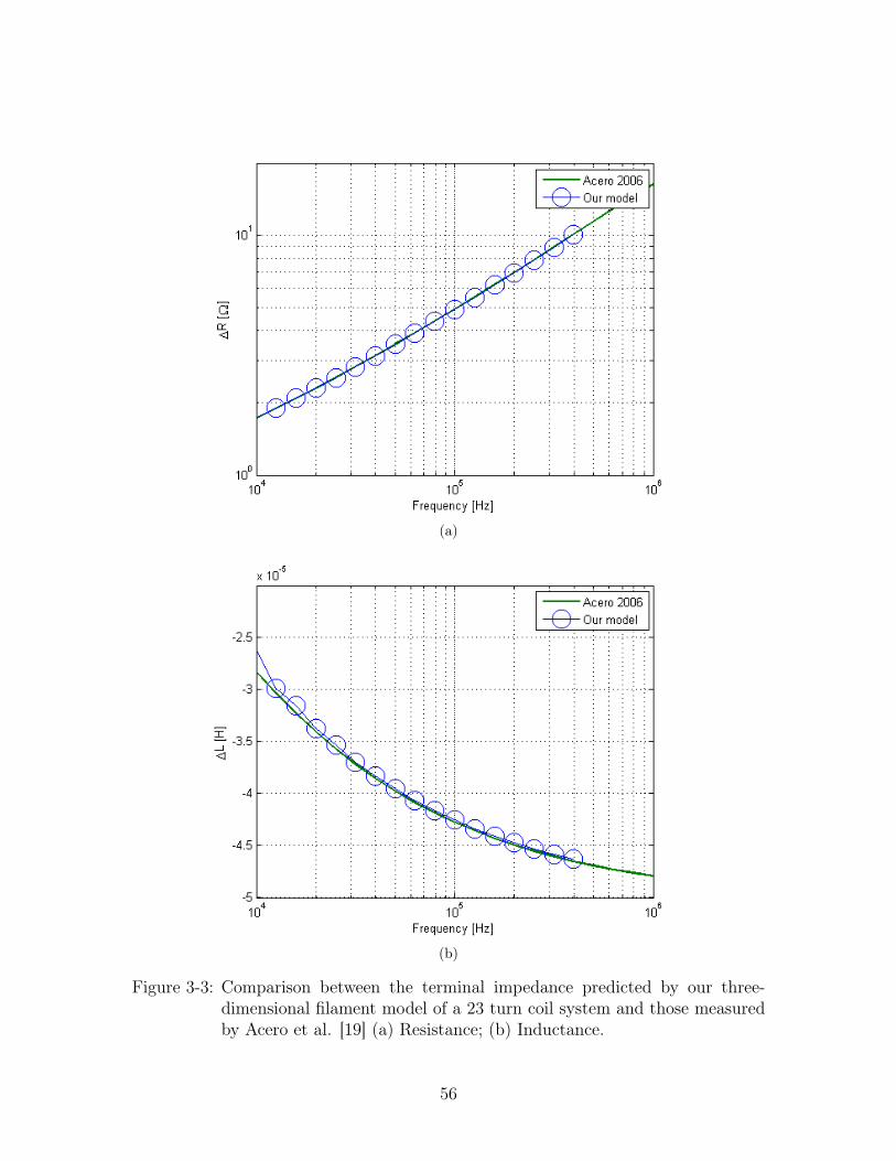
(a)

(b)

Figure 3-3: Comparison between the terminal impedance predicted by our three-dimensional filament model of a 23 turn coil system and those measuredby Acero et al. [19] (a) Resistance; (b) Inductance.

56

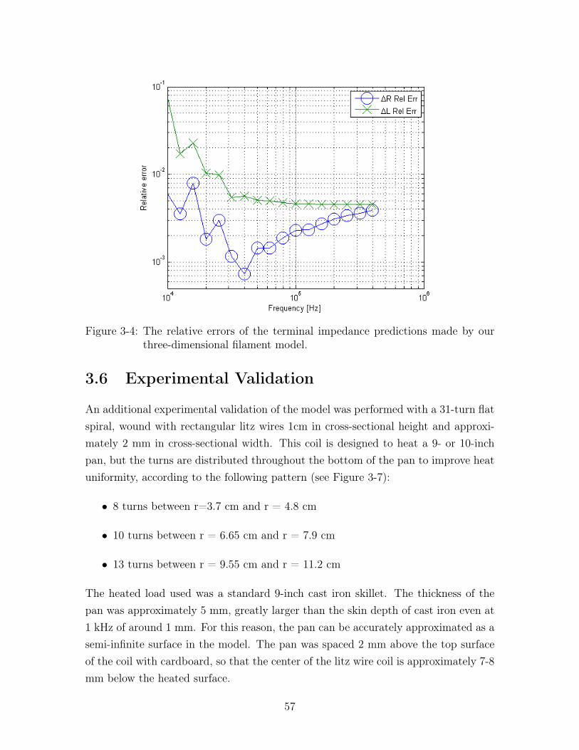
Figure 3-4: The relative errors of the terminal impedance predictions made by ourthree-dimensional filament model.

3.6 Experimental Validation

An additional experimental validation of the model was performed with a 31-turn flatspiral, wound with rectangular litz wires 1cm in cross-sectional height and approxi-mately 2 mm in cross-sectional width. This coil is designed to heat a 9- or 10-inchpan, but the turns are distributed throughout the bottom of the pan to improve heatuniformity, according to the following pattern (see Figure 3-7):

• 8 turns between r=3.7 cm and r = 4.8 cm

• 10 turns between r = 6.65 cm and r = 7.9 cm

• 13 turns between r = 9.55 cm and r = 11.2 cm

The heated load used was a standard 9-inch cast iron skillet. The thickness of thepan was approximately 5 mm, greatly larger than the skin depth of cast iron even at1 kHz of around 1 mm. For this reason, the pan can be accurately approximated as asemi-infinite surface in the model. The pan was spaced 2 mm above the top surfaceof the coil with cardboard, so that the center of the litz wire coil is approximately 7-8mm below the heated surface.

57

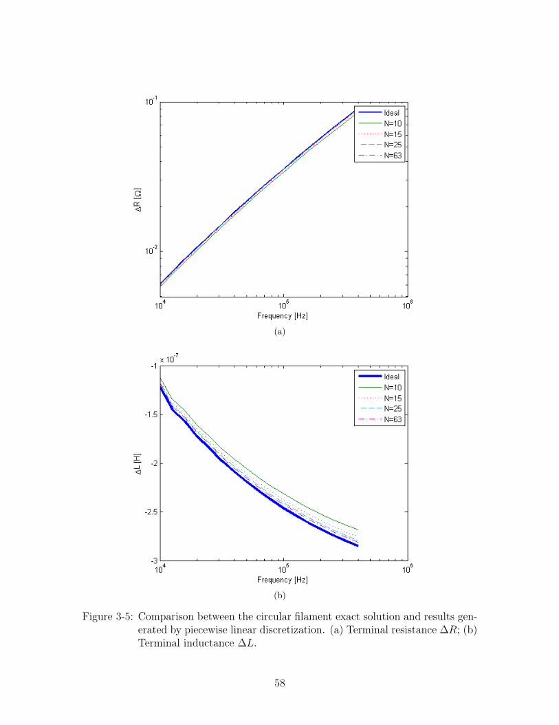
(a)

(b)

Figure 3-5: Comparison between the circular filament exact solution and results gen-erated by piecewise linear discretization. (a) Terminal resistance ∆R; (b)Terminal inductance ∆L.

58

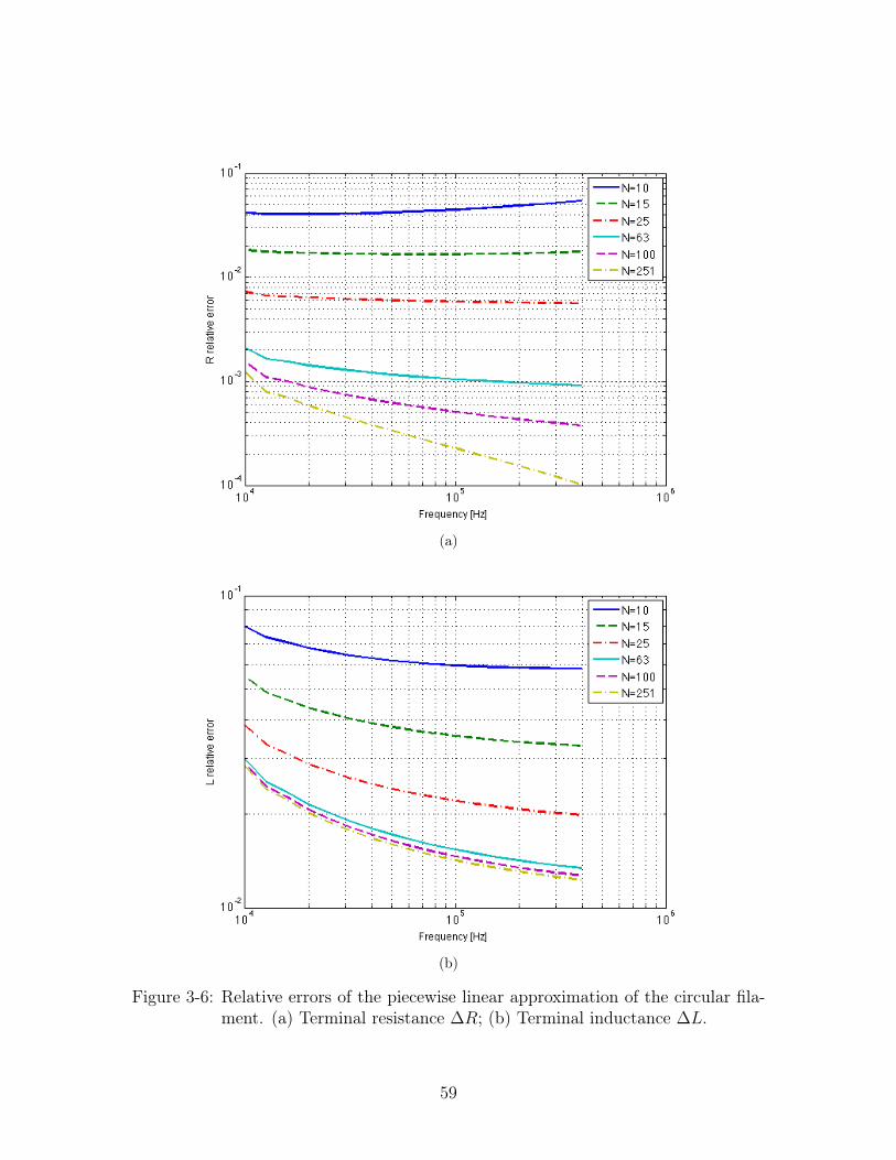
(a)

(b)

Figure 3-6: Relative errors of the piecewise linear approximation of the circular fila-ment. (a) Terminal resistance ∆R; (b) Terminal inductance ∆L.

59

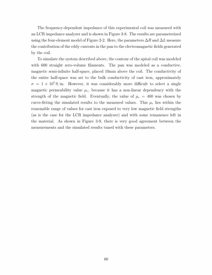
The frequency-dependent impedance of this experimental coil was measured withan LCR impedance analyzer and is shown in Figure 3-8. The results are parameterizedusing the four-element model of Figure 2-2. Here, the parameters ∆R and ∆Lmeasurethe contribution of the eddy currents in the pan to the electromagnetic fields generatedby the coil.

To simulate the system described above, the contour of the spiral coil was modeledwith 600 straight zero-volume filaments. The pan was modeled as a conductive,magnetic semi-infinite half-space, placed 10mm above the coil. The conductivity ofthe entire half-space was set to the bulk conductivity of cast iron, approximatelyσ = 1 × 107 S/m. However, it was considerably more difficult to select a singlemagnetic permeability value µr, because it has a non-linear dependency with thestrength of the magnetic field. Eventually, the value of µr = 400 was chosen bycurve-fitting the simulated results to the measured values. This µr lies within thereasonable range of values for cast iron exposed to very low magnetic field strengths(as is the case for the LCR impedance analyzer) and with some remanence left inthe material. As shown in Figure 3-9, there is very good agreement between themeasurements and the simulated results tuned with these parameters.

60

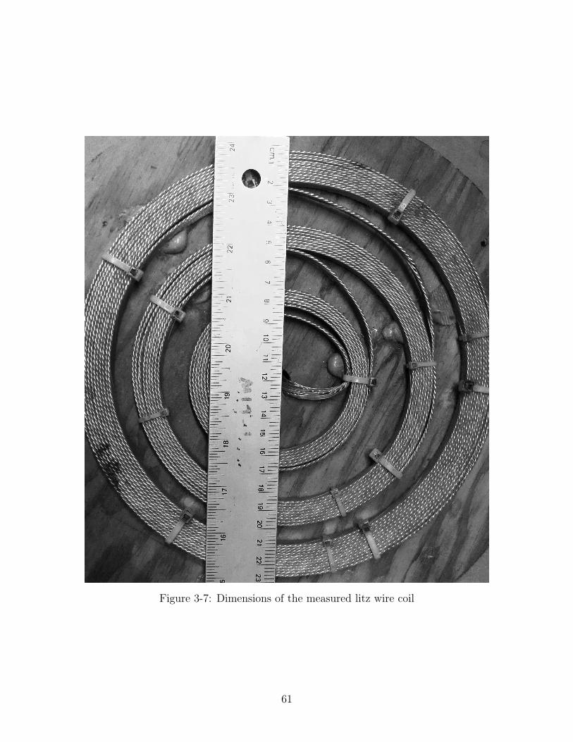
Figure 3-7: Dimensions of the measured litz wire coil

61

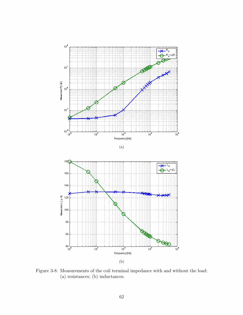
(a)

(b)

Figure 3-8: Measurements of the coil terminal impedance with and without the load:(a) resistances; (b) inductances.

62

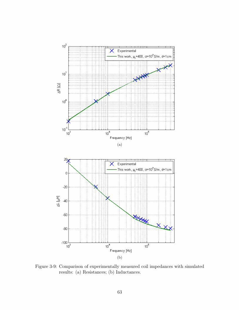
(a)

(b)

Figure 3-9: Comparison of experimentally measured coil impedances with simulatedresults: (a) Resistances; (b) Inductances.

63

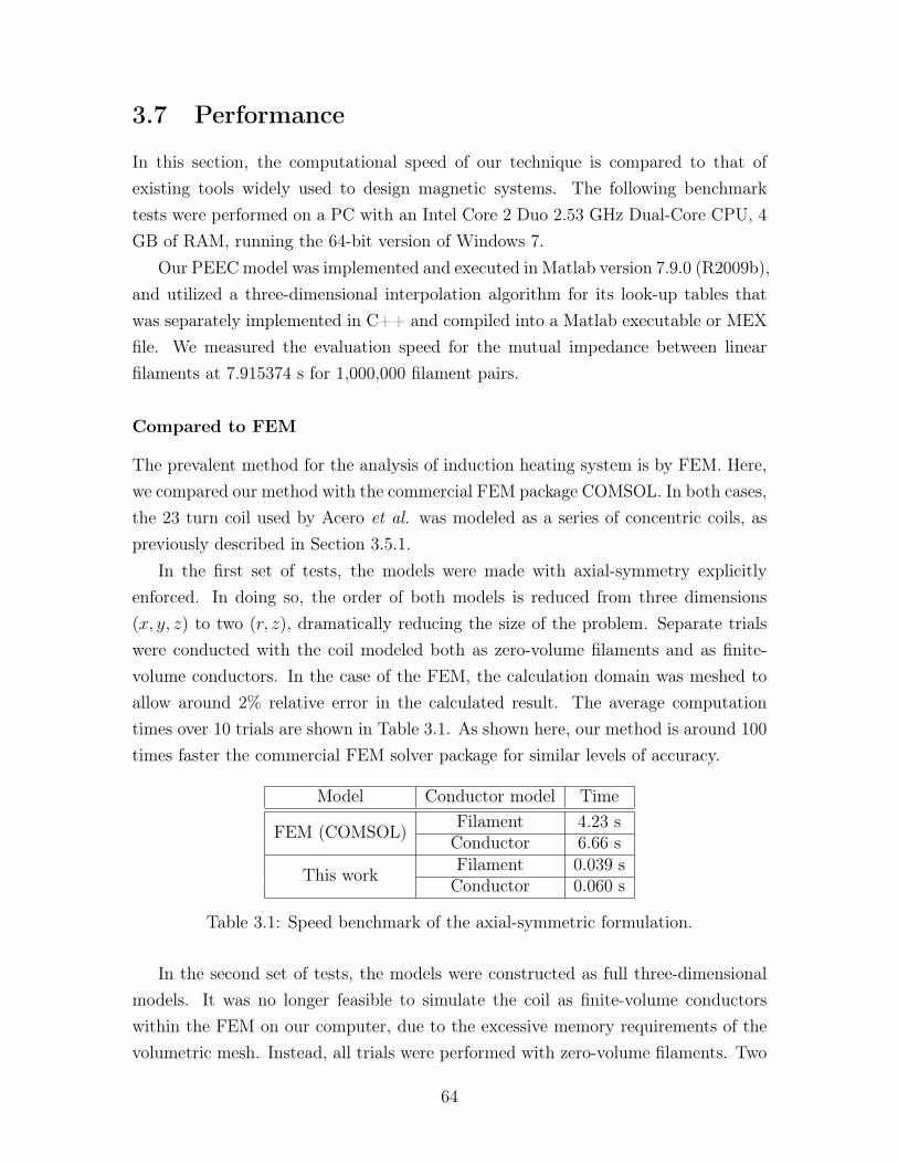
3.7 Performance

In this section, the computational speed of our technique is compared to that ofexisting tools widely used to design magnetic systems. The following benchmarktests were performed on a PC with an Intel Core 2 Duo 2.53 GHz Dual-Core CPU, 4GB of RAM, running the 64-bit version of Windows 7.

Our PEECmodel was implemented and executed in Matlab version 7.9.0 (R2009b),and utilized a three-dimensional interpolation algorithm for its look-up tables thatwas separately implemented in C++ and compiled into a Matlab executable or MEXfile. We measured the evaluation speed for the mutual impedance between linearfilaments at 7.915374 s for 1,000,000 filament pairs.

Compared to FEM

The prevalent method for the analysis of induction heating system is by FEM. Here,we compared our method with the commercial FEM package COMSOL. In both cases,the 23 turn coil used by Acero et al. was modeled as a series of concentric coils, aspreviously described in Section 3.5.1.

In the first set of tests, the models were made with axial-symmetry explicitlyenforced. In doing so, the order of both models is reduced from three dimensions(x, y, z) to two (r, z), dramatically reducing the size of the problem. Separate trialswere conducted with the coil modeled both as zero-volume filaments and as finite-volume conductors. In the case of the FEM, the calculation domain was meshed toallow around 2% relative error in the calculated result. The average computationtimes over 10 trials are shown in Table 3.1. As shown here, our method is around 100times faster the commercial FEM solver package for similar levels of accuracy.

Model Conductor model Time

FEM (COMSOL) Filament 4.23 sConductor 6.66 s

This work Filament 0.039 sConductor 0.060 s

Table 3.1: Speed benchmark of the axial-symmetric formulation.

In the second set of tests, the models were constructed as full three-dimensionalmodels. It was no longer feasible to simulate the coil as finite-volume conductorswithin the FEM on our computer, due to the excessive memory requirements of thevolumetric mesh. Instead, all trials were performed with zero-volume filaments. Two

64

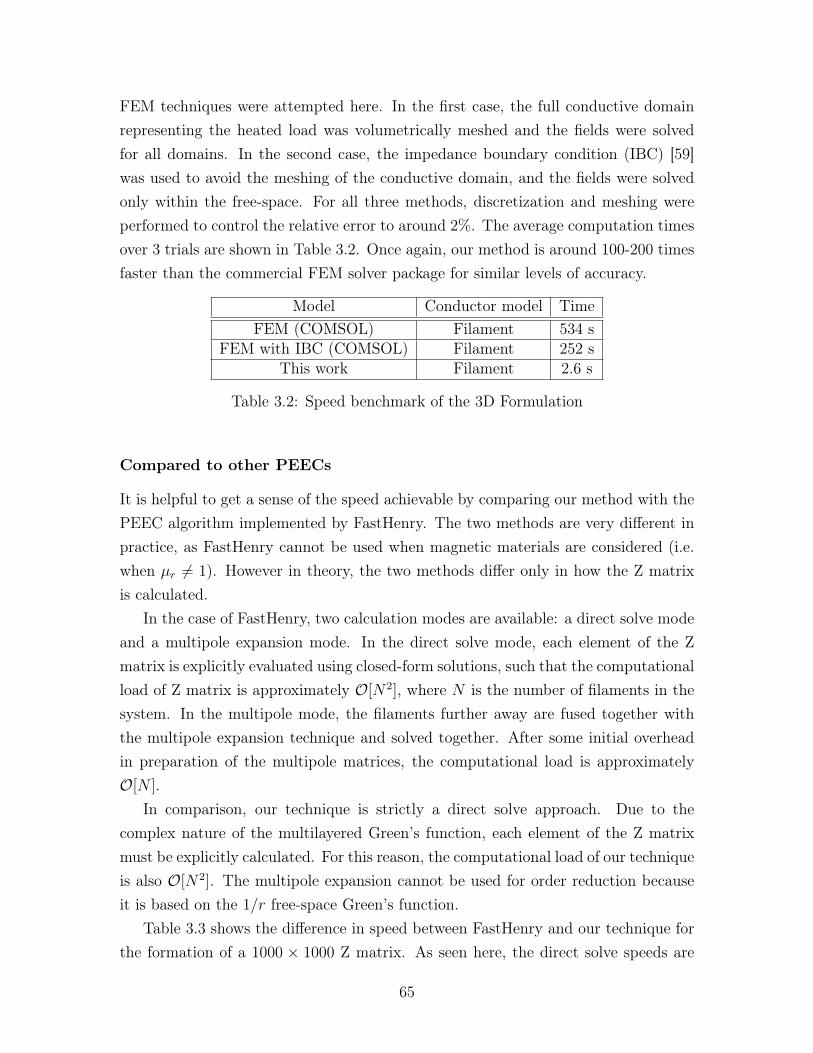
FEM techniques were attempted here. In the first case, the full conductive domainrepresenting the heated load was volumetrically meshed and the fields were solvedfor all domains. In the second case, the impedance boundary condition (IBC) [59]was used to avoid the meshing of the conductive domain, and the fields were solvedonly within the free-space. For all three methods, discretization and meshing wereperformed to control the relative error to around 2%. The average computation timesover 3 trials are shown in Table 3.2. Once again, our method is around 100-200 timesfaster than the commercial FEM solver package for similar levels of accuracy.

Model Conductor model TimeFEM (COMSOL) Filament 534 s

FEM with IBC (COMSOL) Filament 252 sThis work Filament 2.6 s

Table 3.2: Speed benchmark of the 3D Formulation

Compared to other PEECs

It is helpful to get a sense of the speed achievable by comparing our method with thePEEC algorithm implemented by FastHenry. The two methods are very different inpractice, as FastHenry cannot be used when magnetic materials are considered (i.e.when µr 6= 1). However in theory, the two methods differ only in how the Z matrixis calculated.

In the case of FastHenry, two calculation modes are available: a direct solve modeand a multipole expansion mode. In the direct solve mode, each element of the Zmatrix is explicitly evaluated using closed-form solutions, such that the computationalload of Z matrix is approximately O[N2], where N is the number of filaments in thesystem. In the multipole mode, the filaments further away are fused together withthe multipole expansion technique and solved together. After some initial overheadin preparation of the multipole matrices, the computational load is approximatelyO[N ].

In comparison, our technique is strictly a direct solve approach. Due to thecomplex nature of the multilayered Green’s function, each element of the Z matrixmust be explicitly calculated. For this reason, the computational load of our techniqueis also O[N2]. The multipole expansion cannot be used for order reduction becauseit is based on the 1/r free-space Green’s function.

Table 3.3 shows the difference in speed between FastHenry and our technique forthe formation of a 1000 × 1000 Z matrix. As seen here, the direct solve speeds are

65

comparable between the two methods. However, the multipole expansion is able toreduce computation time by around 500, making FastHenry significantly faster thanour technique. This computational advantage is a strong incentive for compressiontechniques (similar to the multipole expansion) to be adopted. The possible can-didates include pre-corrected FFT [60], singular value decomposition [29] and andpartial reluctances [61].

Model Time to evaluate 1,000,000 filament pairsFastHenry (Direct Solve) 2.486 sFastHenry (Multipole) 0.005 s

This work 7.9 s

Table 3.3: Comparison of mutual impedance computation speeds with establishedPEEC tools

66

Chapter 4

Optimal Design of an InductionCooktop

The following chapter presents a design procedure for an induction cooking coil basedupon mathematical single- and multiple-objective optimization algorithms. Similarapproaches with optimization algorithms had been applied to the Transverse-FluxHeating (TFH) of metal strips [62, 36], the rapid heating of an injection mold plate[63], the design of a passive and active induction heating shield [33], and the design ofan induction cooker [14]. In formulating their optimization strategies, these previousauthors have placed heavy emphasis upon obtaining a uniform temperature profilein the heated load. For this reason, finite element method (FEM) models were usedin many of these studies to capture the non-linear temperature- and field-dependentmaterial effects. While highly accurate, FEM is unfortunately a very computationallyexpensive approach: each individual FEM evaluation can take from a few minutes toa few hours to complete. As a result, only relatively basic optimization techniqueshave been applied with relatively few degrees of freedom explored [4].

In the following chapter, the Partial Element Equivalent Circuit (PEEC) methoddeveloped in Chapter 3 is used in lieu of the FEM to evaluate and assess the perfor-mance of proposed coil designs. By reducing the run time from several minutes to lessthan 5 seconds for each coil evaluated, our PEEC method allows optimization to beperformed with more advanced algorithms than those previously used for inductionheating in the literature, and also over many more degrees of freedom than tradition-ally afforded. In particular, the simulated annealing algorithm [64] is used to find theglobal optimum for the single-objective problem, and the NSGA-II multi-objectivegenetic algorithm [65] is used to study the multiple-objective problem.

67

4.1 The Fitness Function

In computational design and optimization, the analyzed problem is typically posedas three distinct components:

1. An encoding / decoding algorithm that translates the vector of numbers rep-resenting points in the design space into physical designs understood by thesoftware model.

2. A software model that simulates the physics of each design.

3. A scoring algorithm that analyzes the results of the software model and assignsfitness scores for the optimization algorithm to optimize.

Combined in series, these three components form what is known as the fitness func-tion: a function that takes in a vector of numbers and outputs a set of fitness scores.The optimization algorithm is then tasked with the sole job of finding the vector ofnumbers that will minimize the fitness function.

4.1.1 Encoding Algorithm

Beyond simply summarizing the physical system into design degrees of freedom thatcan be vectorized and processed by a numerical optimization algorithm, the designof the encoding algorithm also shapes the fitness function within the design space.If the fitness function is shaped with fewer peaks and smoother, gentler gradients,then optimization algorithms will have an easier time traversing the design space andconverging to the global optimum.

The approached used in this chapter is to constrain the coil to a spiral-path design,one that can be mathematically defined with the radius and height of the path asfunctions of the angle of rotation θ. For a spiral of N turns, the encoding methoddefines the input vector x as

x =

N

r0

z0

r1

z1

...rm

zm

(4.1)

68

where r0 · · · rm, z0 · · · zm are the radial and height functions r(θ) and z(θ), sampleduniformly with respect to θ. The starting points r0 and z0 are matched with r(θ = 0)

and z(θ = 0) and the ending points rm and zm are matched with r(θ = 2πN) andz(θ = 2πN). Additional turns can be added by incrementing the N parameter of thex vector. Defining the subscript k ∈ N : 0 ≤ k ≤ m, one can write

rk = r(k · 2πN

m), zk = z(k · 2πN

m) (4.2)

The encoding algorithm then generates P linear piece-wise filaments to approx-imate the spiral, by uniformly resampling both r(θ) and z(θ) to P + 1 points withcubic spline interpolation, and by generating linear filaments to connect these pointstogether sequentially. This way, areas closer to the center of the spiral are modeledwith shorter filaments than those further away, to ensure that parts of the coil withgreater curvature gradients are more finely meshed.

Some additional modifications to this encoding scheme were added to improvethe shape of the fitness function. Firstly, the sampled rk values (but not zk) valuesare sorted to make the resultant radius function r(θ) monotonically increasing withrespect to θ. Secondly, all values of x are normalized to lie within the range of 0 and1 so that the bounded constraint can be readily applied to fix each coil parameterwithin sensible values.

4.1.2 The Electromagnetic Model

Given a set of conductive filaments, the PEEC model developed in Chapter 3 can beused to efficiently solve for the electromagnetic fields and heating fluxes within thesystem. Within the framework of the PEEC model, the coil system is modeled as thefollowing:

• The z axis points in the upwards direction.

• Two semi-infinite half-spaces are defined with

– free-space and the induction coil in the z > 0 region,

– the pan modeled as a custom-defined conductive magnetic material in thez < 0 region and

– the plane z = 0 defined as the interface surface of interaction.

• The x and y axes are defined orthogonal to the z axis, on the surface of inter-action.

69

• Linear filaments of arbitrary lengths and angles of rotation and inclination aregenerated, contained within the 4 < z < 20 mm and −20 < x, y < +20 cm boxregion.

While fast and efficient, the PEEC model does makes several approximations in pur-suit of computational speed. The model requires everything to be linear by its inher-ent formulation, and so cannot accommodate properties that are field or temperaturedependent. This effectively eliminates hysteresis as a loss mechanism. This is accept-able in the great majority of induction heating applications, because the heat effectdue to hysteresis does not typically exceed 7% compared to the heat effect due toeddy current losses [66].

Another approximation made to enhance speed is to model the finite-volume con-ductors as zero-volume, point to point filaments. It was the empirical experience ofthe author and other works in literature such as [37] that optimization objectiveswithin this thesis are not strongly affected by the cross-sectional area of the conduc-tor itself. If necessary, the PEEC tool can also be used to simulate finite-volumeconductors, although the computational cost of this is high and so was not pursuedfurther.

4.1.3 Scoring Algorithm

The three major conflicting objectives for the design of the induction cooker coil arethe cost of the coil, its efficiency and the resultant heat profile that it produces. Afterevaluating the fields for each coil design, the scoring algorithm should assign it threescores, one based on each of these three criteria. All the optimization algorithms usedare minimizing algorithms (i.e. lower is better); where it is desired for a particularscore to be maximized instead, the score can be inverted by multiplying with −1.

Cost

In a mass-production environment, the largest variable cost is the coil material itself.Holding the cross-sectional area of the wire used constant, a longer coil requires morecopper to construct, and therefore will always cost more to manufacture. Here, thelength of the coil is used as a proxy to rank the designs by their production costs.

70

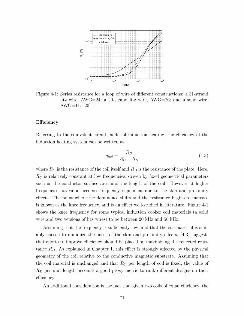
Figure 4-1: Series resistance for a loop of wire of different constructions: a 31-strandlitz wire, AWG=24; a 20-strand litz wire, AWG=26; and a solid wire,AWG=11. [20]

Efficiency

Referring to the equivalent circuit model of induction heating, the efficiency of theinduction heating system can be written as

ηind =RD

RC +RD

(4.3)

where RC is the resistance of the coil itself and RD is the resistance of the plate. Here,RC is relatively constant at low frequencies, driven by fixed geometrical parameterssuch as the conductor surface area and the length of the coil. However at higherfrequencies, its value becomes frequency dependent due to the skin and proximityeffects. The point where the dominance shifts and the resistance begins to increaseis known as the knee frequency, and is an effect well-studied in literature. Figure 4-1shows the knee frequency for some typical induction cooker coil materials (a solidwire and two versions of litz wires) to be between 20 kHz and 50 kHz.

Assuming that the frequency is sufficiently low, and that the coil material is suit-ably chosen to minimize the onset of the skin and proximity effects, (4.3) suggeststhat efforts to improve efficiency should be placed on maximizing the reflected resis-tance RD. As explained in Chapter 1, this effect is strongly affected by the physicalgeometry of the coil relative to the conductive magnetic substrate. Assuming thatthe coil material is unchanged and that RC per length of coil is fixed, the value ofRD per unit length becomes a good proxy metric to rank different designs on theirefficiency.

An additional consideration is the fact that given two coils of equal efficiency, the

71

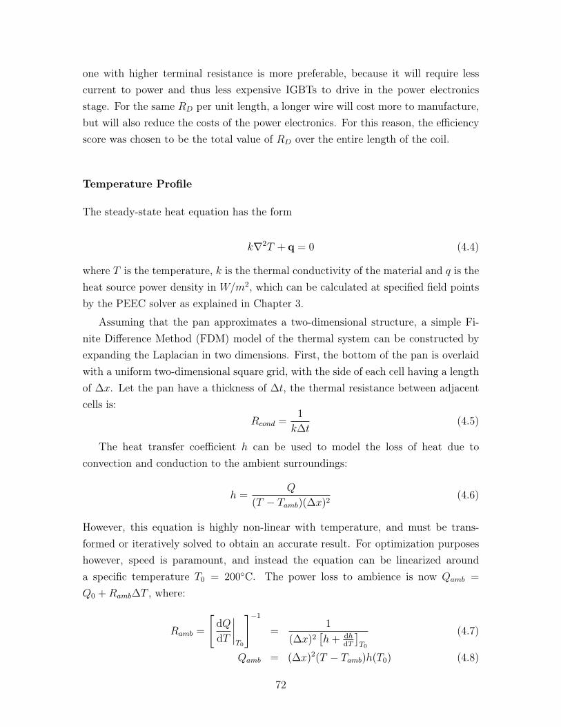
one with higher terminal resistance is more preferable, because it will require lesscurrent to power and thus less expensive IGBTs to drive in the power electronicsstage. For the same RD per unit length, a longer wire will cost more to manufacture,but will also reduce the costs of the power electronics. For this reason, the efficiencyscore was chosen to be the total value of RD over the entire length of the coil.

Temperature Profile

The steady-state heat equation has the form

k∇2T + q = 0 (4.4)

where T is the temperature, k is the thermal conductivity of the material and q is theheat source power density in W/m2, which can be calculated at specified field pointsby the PEEC solver as explained in Chapter 3.

Assuming that the pan approximates a two-dimensional structure, a simple Fi-nite Difference Method (FDM) model of the thermal system can be constructed byexpanding the Laplacian in two dimensions. First, the bottom of the pan is overlaidwith a uniform two-dimensional square grid, with the side of each cell having a lengthof ∆x. Let the pan have a thickness of ∆t, the thermal resistance between adjacentcells is:

Rcond =1

k∆t(4.5)

The heat transfer coefficient h can be used to model the loss of heat due toconvection and conduction to the ambient surroundings:

h =Q

(T − Tamb)(∆x)2(4.6)

However, this equation is highly non-linear with temperature, and must be trans-formed or iteratively solved to obtain an accurate result. For optimization purposeshowever, speed is paramount, and instead the equation can be linearized arounda specific temperature T0 = 200C. The power loss to ambience is now Qamb =

Q0 +Ramb∆T , where:

Ramb =

[dQ

dT

∣∣∣∣T0

]−1

=1

(∆x)2[h+ dh

dT

]T0

(4.7)

Qamb = (∆x)2(T − Tamb)h(T0) (4.8)

72

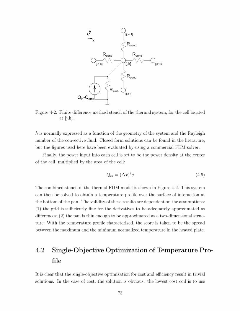
Rcond

Rcond

RcondRcond

Ramb

[j,k]

[j,k+1]

[j,k-1]

[j+1,k][j-1,k]

x

y

Qin-Qamb

Figure 4-2: Finite difference method stencil of the thermal system, for the cell locatedat [j,k].

h is normally expressed as a function of the geometry of the system and the Rayleighnumber of the convective fluid. Closed form solutions can be found in the literature,but the figures used here have been evaluated by using a commercial FEM solver.

Finally, the power input into each cell is set to be the power density at the centerof the cell, multiplied by the area of the cell:

Qin = (∆x)2q (4.9)

The combined stencil of the thermal FDM model is shown in Figure 4-2. This systemcan then be solved to obtain a temperature profile over the surface of interaction atthe bottom of the pan. The validity of these results are dependent on the assumptions:(1) the grid is sufficiently fine for the derivatives to be adequately approximated asdifferences; (2) the pan is thin enough to be approximated as a two-dimensional struc-ture. With the temperature profile characterized, the score is taken to be the spreadbetween the maximum and the minimum normalized temperature in the heated plate.

4.2 Single-Objective Optimization of Temperature Pro-

file

It is clear that the single-objective optimization for cost and efficiency result in trivialsolutions. In the case of cost, the solution is obvious: the lowest cost coil is to use

73

no coil at all; for high efficiency, the best coil is the one with as many large turns aspossible, as close as possible to the heated surface.

By contrast, it is non-trivial to design an induction heating coil to achieve auniform temperature profile. The single-objective optimization of the temperatureprofile is inherently non-linear, because it cannot be posed in a way for the objectivefunction to be formulated as a linear combination of input variables, subject to linearconstraints. In the following section, a two-part simulated annealing / hybrid patternsearch algorithm is used to perform the single-objective optimization of the loadtemperature profile.

The optimization strategy used combines the ability of statistical methods to breakaway from local stationary points and converge towards global minimums, with thefast convergence speed of traditional algorithmic search techniques. In the first stageof the optimization, simulated annealing is chosen over genetic algorithms and otherstatistical methods for its mathematically sufficient ability to converge towards theglobal minimum given enough iterations1. The search is initiated with a 23-turn flatcoil design from [19, 20, 11], shown in Figure 4-3. The radius of this initial coil is from2.5 to 10.5 cm, and it is placed at a distance of 4mm from the load. The scheme usesBoltzmann Annealing to guarantee convergence towards the global optimum, and has13 degrees of freedom: one that allows the number of turns to vary from 0 to 23, andthe other twelve to define the radius function r(θ) and the height function z(θ). Theencoder generates 600 linear filaments, and the heat profile is evaluated for a 30× 30

square grid in the z = 0 plane, spanning x, y = ±0.15 m. Bicubically interpolatingbetween these values, the temperature profile is calculated using the FDM schemedescribed above.

After 2500 iterations of simulated annealing, the normalized temperature spreaddrops from 11% in the initial design to 4%, which is an improvement of almost three.The resultant coil is shown in Figure 4-4. In the second stage of the optimization, amixed general pattern search / Nelder-Mead simplex-method search is performed toconverge upon the optimum point found by the simulated annealing algorithm. Thesearch begins with the design found at the end of the simulated annealing algorithm.It then polls the design points around it according to pattern search rules and alsoaccording to the Nelder-Mead simplex-method rules [67]. If any of these polled pointsperform better than the original point, it is chosen as the newest best design, and thesame process is repeated. Given that the step sizes are sufficiently small, the local

1An extensive discussion of the algorithm, the relevant terminology and its history can be foundin [17].

74

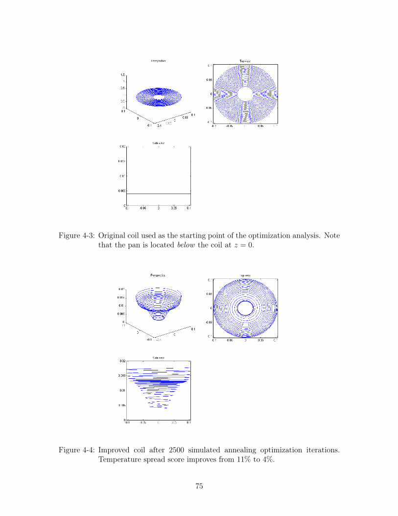
Figure 4-3: Original coil used as the starting point of the optimization analysis. Notethat the pan is located below the coil at z = 0.

Figure 4-4: Improved coil after 2500 simulated annealing optimization iterations.Temperature spread score improves from 11% to 4%.

75

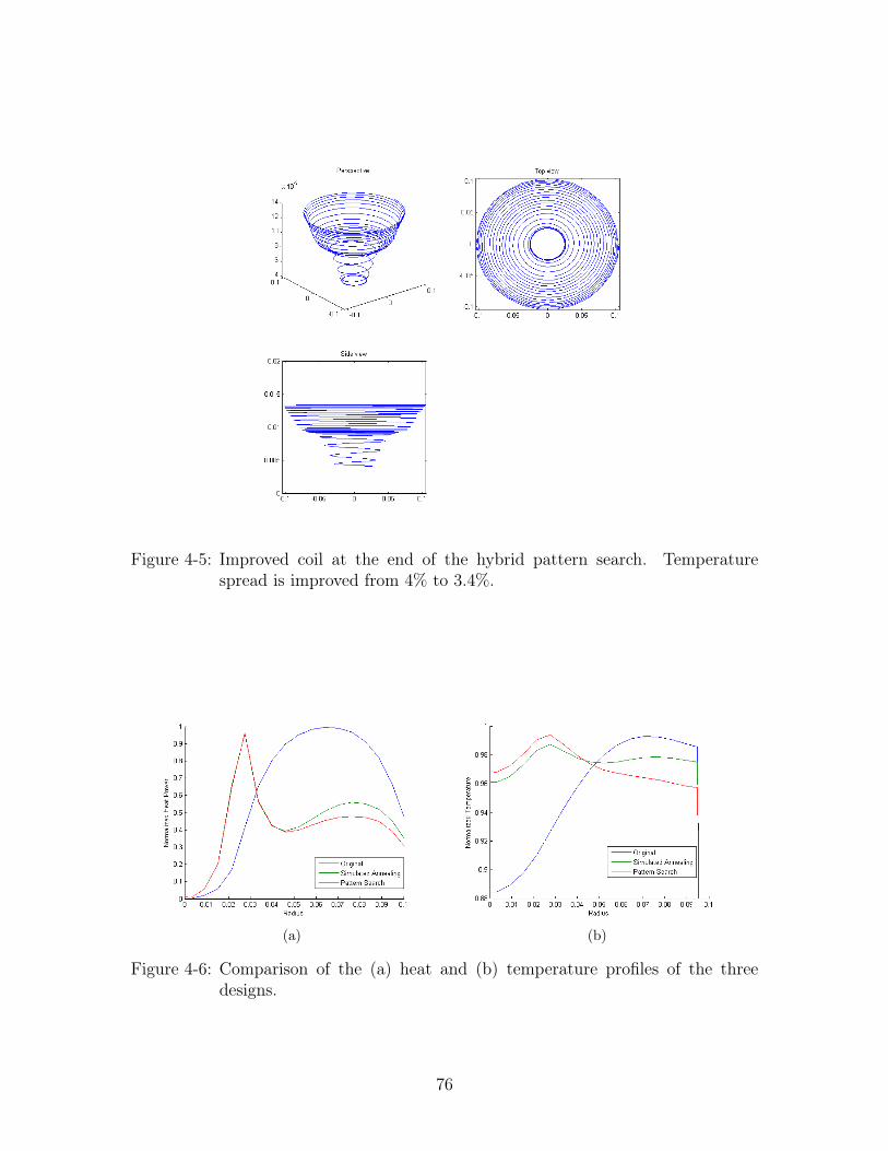
Figure 4-5: Improved coil at the end of the hybrid pattern search. Temperaturespread is improved from 4% to 3.4%.

(a) (b)

Figure 4-6: Comparison of the (a) heat and (b) temperature profiles of the threedesigns.

76

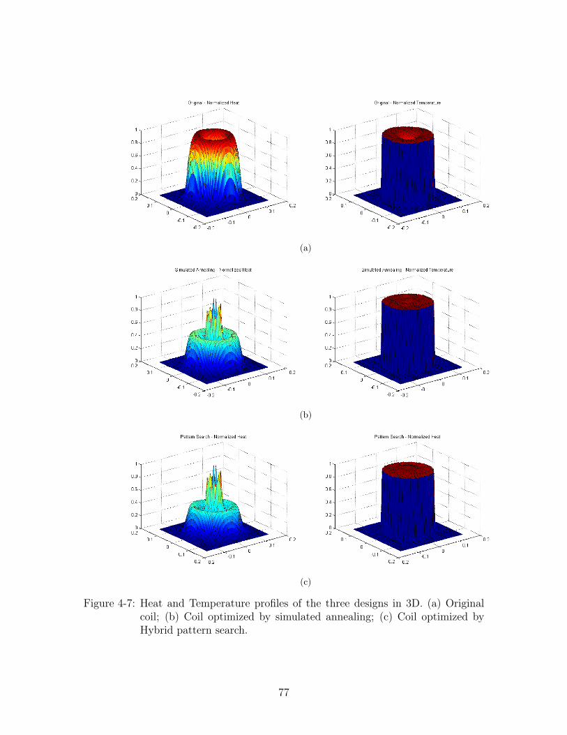
(a)

(b)

(c)

Figure 4-7: Heat and Temperature profiles of the three designs in 3D. (a) Originalcoil; (b) Coil optimized by simulated annealing; (c) Coil optimized byHybrid pattern search.

77

region around the starting point is expected to be convex. If this is indeed the case,then the hybrid method is sufficient for convergence to the true optimum. After 65iterations, the hybrid method improves the temperature spread further from 4% to3.4%. The improved design is shown in Figure 4-5.

Figure 4-6 shows the heat and temperature profiles of the three designs as cross-sectional slices in the z-r plane, starting from the center. Figure 4-7 shows thesesame results as three-dimensional surfaces. Seen here, a significant impediment to auniform temperature profile is the coil’s inability to heat the center of the load, anobservation that agrees with other authors [14, 63]. The radius and height functionsand their sampled values are plotted in Figure 4-8. As expected, the optimizationalgorithm has placed more turns of the coil towards the center and closer to theload in order to address the weaker heating ability there. However, an unexpectedinnovation found by the optimization algorithm is to placed the outer turns furtheraway from the load in the z direction.

4.3 Multi-Objective Optimization of Temperature,

Efficiency and Cost

An optimization problem is said to be multi-objective when more than one cost orscore function is considered. In this case, there is rarely an absolutely optimal so-lution, one that simultaneously out-performs all other solutions in all criteria. Forexample, there is no unique coil design that could simultaneously minimize cost, andmaximize efficiency and temperature uniformity, due to the conflicting nature of theseobjectives. Instead, the goal is to discover a set of solutions at the trade-off bound-aries between the different objectives, and to select one of these optimized solutionsaccording to designer preferences. [68]

The solutions of multi-objective optimization are formally known as Pareto op-timal solutions. A solution is considered to be Pareto optimal when it cannot bemodified to improve its performance in one design objective without adversely af-fecting its performance in other objectives. By contrast, a non-Pareto optimal or adominated solution is one that can be non-subjectively improved. For example a coildesign that can be modified to be more efficient while still costing the same amountto manufacture is said to be dominated by the modified design, and is non-Paretooptimal.

A wide range of methods have been developed to solve the multi-objective opti-

78

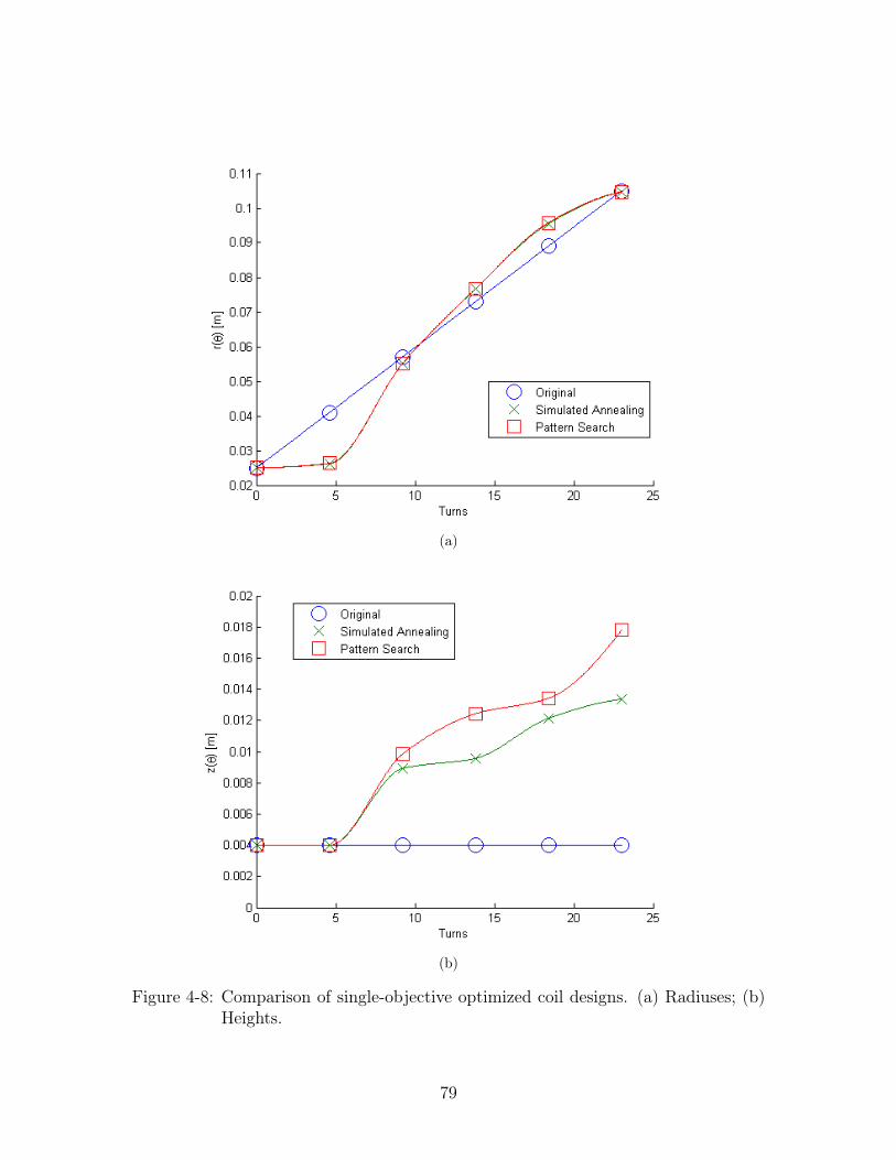
(a)

(b)

Figure 4-8: Comparison of single-objective optimized coil designs. (a) Radiuses; (b)Heights.

79

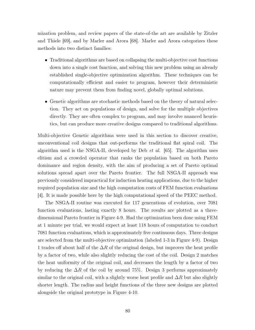
mization problem, and review papers of the state-of-the art are available by Zitzlerand Thiele [69], and by Marler and Arora [68]. Marler and Arora categorizes thesemethods into two distinct families:

• Traditional algorithms are based on collapsing the multi-objective cost functionsdown into a single cost function, and solving this new problem using an alreadyestablished single-objective optimization algorithm. These techniques can becomputationally efficient and easier to program, however their deterministicnature may prevent them from finding novel, globally optimal solutions.

• Genetic algorithms are stochastic methods based on the theory of natural selec-tion. They act on populations of design, and solve for the multiple objectivesdirectly. They are often complex to program, and may involve nuanced heuris-tics, but can produce more creative designs compared to traditional algorithms.

Multi-objective Genetic algorithms were used in this section to discover creative,unconventional coil designs that out-performs the traditional flat spiral coil. Thealgorithm used is the NSGA-II, developed by Deb et al. [65]. The algorithm useselitism and a crowded operator that ranks the population based on both Paretodominance and region density, with the aim of producing a set of Pareto optimalsolutions spread apart over the Pareto frontier. The full NSGA-II approach waspreviously considered impractical for induction heating applications, due to the higherrequired population size and the high computation costs of FEM function evaluations[4]. It is made possible here by the high computational speed of the PEEC method.

The NSGA-II routine was executed for 117 generations of evolution, over 7081function evaluations, lasting exactly 8 hours. The results are plotted as a three-dimensional Pareto frontier in Figure 4-9. Had the optimization been done using FEMat 1 minute per trial, we would expect at least 118 hours of computation to conduct7081 function evaluations, which is approximately five continuous days. Three designsare selected from the multi-objective optimization (labeled 1-3 in Figure 4-9). Design1 trades off about half of the ∆R of the original design, but improves the heat profileby a factor of two, while also slightly reducing the cost of the coil. Design 2 matchesthe heat uniformity of the original coil, and decreases the length by a factor of twoby reducing the ∆R of the coil by around 75%. Design 3 performs approximatelysimilar to the original coil, with a slightly worse heat profile and ∆R but also slightlyshorter length. The radius and height functions of the three new designs are plottedalongside the original prototype in Figure 4-10.

80

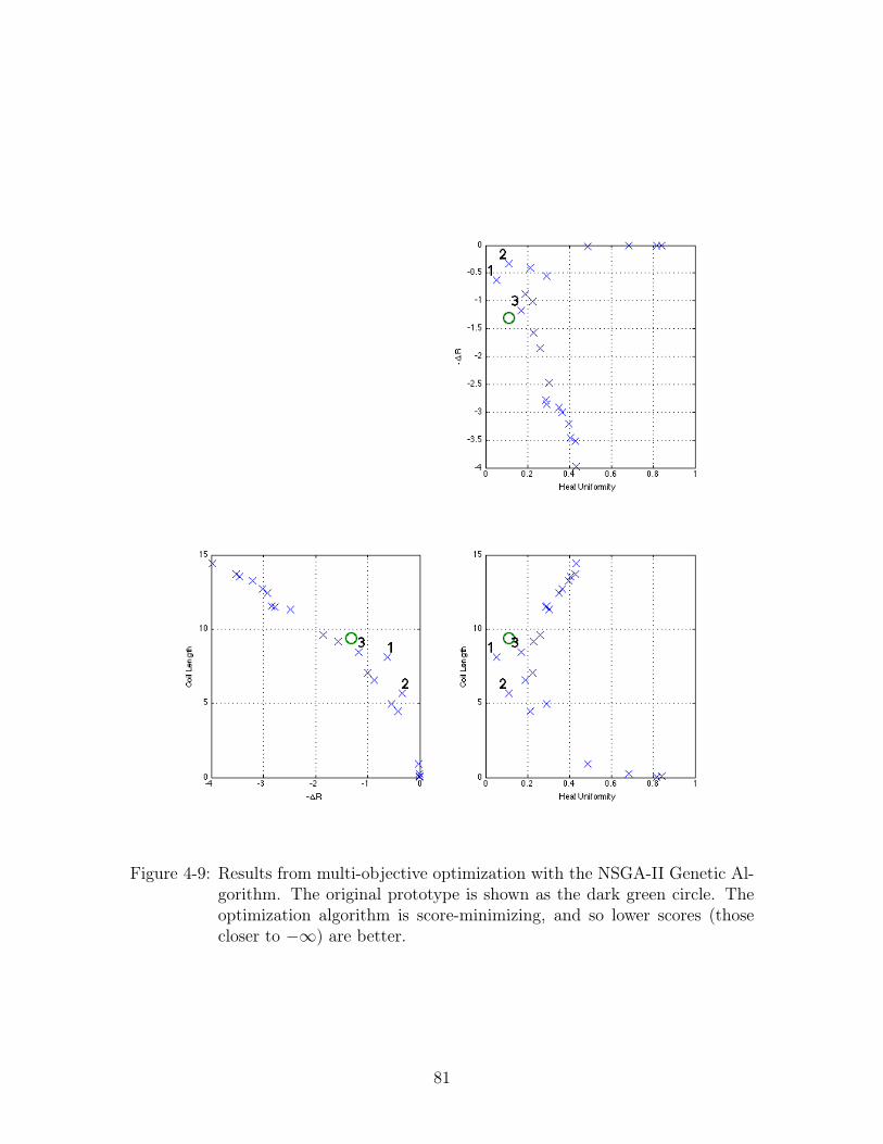
Figure 4-9: Results from multi-objective optimization with the NSGA-II Genetic Al-gorithm. The original prototype is shown as the dark green circle. Theoptimization algorithm is score-minimizing, and so lower scores (thosecloser to −∞) are better.

81

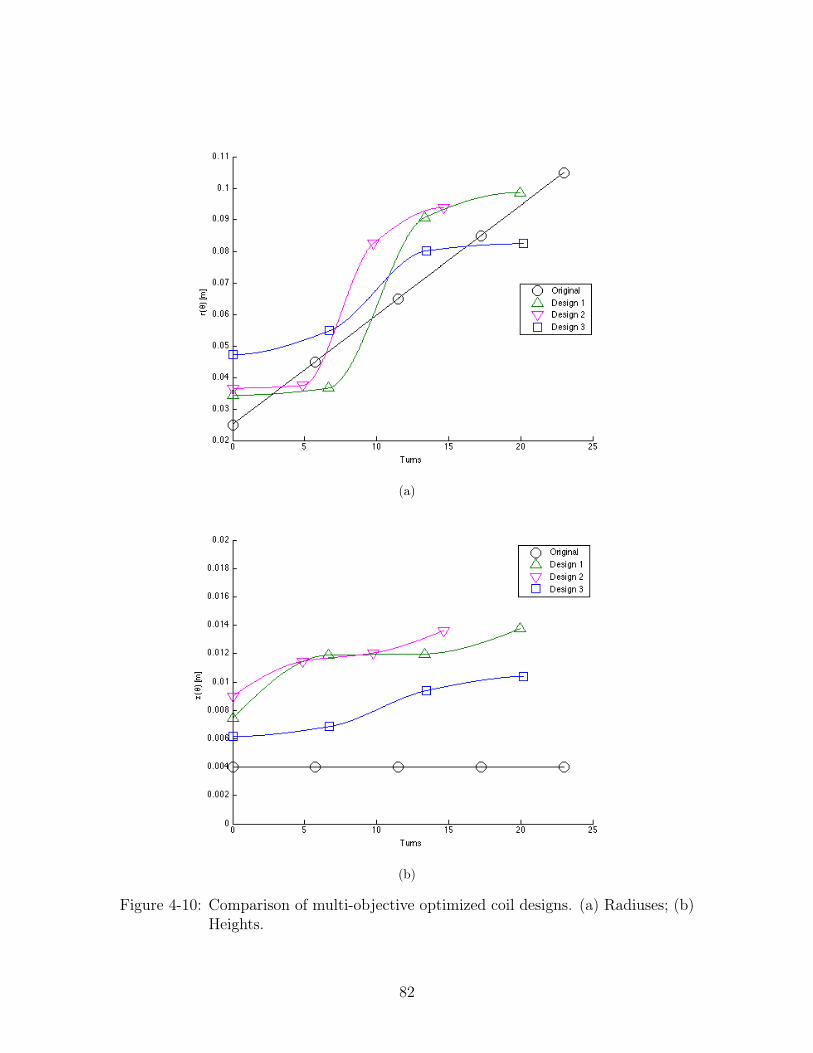
(a)

(b)

Figure 4-10: Comparison of multi-objective optimized coil designs. (a) Radiuses; (b)Heights.

82

Chapter 5

Conclusions and Future Work

In this thesis, it is shown that the multilayer Green’s function derived from the planargeometry of domestic induction heating can be used to substantially accelerate thecomputation of magnetoquasistatic electromagnetic fields. Controlling for similarlevels of relative error, our PEEC solver was able to perform at speeds of 100+ timesfaster than the tested commercial FEM package, an improvement of two orders ofmagnitude.

Our PEEC solver was used to perform the single-objective optimization of theload temperature profile, as well as the multi-objective optimization of the tempera-ture, efficiency and cost. In both cases, the optimization algorithms used–SimulatedAnnealing and NSGA-II–were previously deemed impractical due to the high compu-tational costs of fitness function evaluations. Both optimization algorithms producednovel, three-dimensional induction coil designs.

Further improvements to the results of this thesis can be made in the followingtwo areas:

Compression techniques. The bottleneck of the PEEC method proposedwithin this thesis is the formation of the dense Z matrix, currently formed at com-plexity order O[N2]. Significant speed advantages can be gained by compression /sparsification techniques, such as pre-corrected Fourier transform [60, 70], singularvalue decomposition [29] and partial reluctances [61]. It was shown in Section 3.7that the use of the Fast Multipole Method compression technique reduced the com-plexity of FastHenry to approximately O[N ], and increased its speed by two to threeorders of magnitude.

More comprehensive optimization routines. The optimization routine withinthis thesis retained the spiral property of the induction coil, and applied “vanilla”versions of two popular optimization algorithms. The “no free lunch” theorem of op-

83

timization asserts that no universal optimization algorithm exists that is efficient forall classes of problems [71], and this suggests that further gains can be obtained ifthe algorithms are adapted for their specific applications. Indeed, customized ver-sions of both algorithms are widespread for the induction heating application [4].Improvements on the optimization algorithms could allow more degrees of freedomto be explored in the design of the coil with fewer function evaluations.

84

Bibliography

[1] J. Acero, J. Burdio, L. Barragan, D. Navarro, R. Alonso, J. Garcia, F. Monterde,P. Hernandez, S. Llorente, and I. Garde, “Domestic Induction Appliances,” IEEEIndustry Applications Magazine, vol. 16, no. 2, pp. 39–47, 2010.

[2] A. Fujita, H. Sadakata, I. Hirota, H. Omori, and M. Nakaoka, “Latest Develop-ments of High-Frequency Series Load Resonant Inverter Type Built-In Cooktopsfor Induction Heated All Metallic Appliances,” in IEEE IPEMC ’09, vol. 3, 2009,pp. 2537–2544.

[3] L. Chambers, Ed., The Practical Handbook of Genetic Algorithms: Applications,Second Edition. Chapman and Hall/CRC, 2000.

[4] C. Coello and G. Lamont, Eds., Applications Of Multi-Objective EvolutionaryAlgorithms (Advances in Natural Computation). World Scientific Pub Co Inc,2004.

[5] H. Koertzen, J. van Wyk, and J. Ferreira, “Design of the half-bridge, seriesresonant converter for induction cooking,” in Power Electronics SpecialistsConference, 1995. PESC’95 Record., 26th Annual IEEE, vol. 2. IEEE, 1995,pp. 729–735.

[6] C. Dodd, “Analytical Solutions to Eddy-Current Probe-Coil Problems,” Journalof Applied Physics, vol. 39, no. 6, pp. 2829–2838, 1968.

[7] M. Adler, “A field-theoretical approach to magnetic induction heating of thincircular plates,” IEEE Transactions on Magnetics, vol. 10, no. 4, pp. 1118–1125,Dec. 1974.

[8] W. Hurley and J. Kassakian, “Induction heating of circular ferromagneticplates,” IEEE Transactions on Magnetics, vol. 15, no. 4, pp. 1174–1181, Jul.1979.

[9] W. Roshen and D. Turcotte, “Planar inductors on magnetic substrates,” IEEETransactions on Magnetics, vol. 24, no. 6, pp. 3213–3216, 1988.

[10] W. Roshen, “Effect of finite thickness of magnetic substrate on planarinductors,” IEEE Transactions on Magnetics, vol. 26, no. 1, pp. 270–275, 1990.

85

[11] J. Acero, R. Alonso, L. Barragán, and J. Burdio, “Modeling of planar spiralinductors between two multilayer media for induction heating applications,”Magnetics, IEEE Transactions on, vol. 42, no. 11, pp. 3719–3729, 2006.

[12] J. Acero, R. Alonso, J. M. Burdio, L. a. Barragan, and S. Llorente,“Electromagnetic induction of planar windings with cylindrical symmetrybetween two half-spaces,” Journal of Applied Physics, vol. 103, no. 10, p.104905, 2008.

[13] H. Koertzen, J. van Wyk, and J. Ferreira, “Investigating the influence ofmaterial properties on the efficiency of an induction heating load transformerusing FEM simulations,” in IAS ’95. Conference Record of the 1995 IEEEIndustry Applications Conference Thirtieth IAS Annual Meeting, vol. 1. IEEE,1995, pp. 868–873.

[14] J.-k. Byun, K. Choi, H. Roh, and S.-y. Hahn, “Optimal design procedure for apractical induction heating cooker,” Magnetics, IEEE Transactions on, vol. 36,no. 4, pp. 1390–1393, 2000.

[15] J. Lavers, “State of the art of numerical modeling for induction processes,”COMPEL: The International Journal for Computation and Mathematics inElectrical and Electronic Engineering, vol. 27, no. 2, pp. 335–349, 2008.

[16] A. E. Ruehli, “Inductance Calculations in a Complex Integrated CircuitEnvironment,” IBM Journal of Research and Development, vol. 16, no. 5, pp.470–481, Sep. 1972.

[17] L. Ingber, “Adaptive simulated annealing (ASA): Lessons learned,” Control andCybernetics, 1996.

[18] A. Mühlbauer, “History of induction heating and melting,” 2008.

[19] J. Acero, R. Alonso, J. Burdio, L. Barragán, and D. Puyal, “Analyticalequivalent impedance for a planar circular induction heating system,” Magnetics,IEEE Transactions on, vol. 42, no. 1, pp. 84–86, 2006.

[20] ——, “Frequency-dependent resistance in litz-wire planar windings for domesticinduction heating appliances,” Power Electronics, IEEE Transactions on,vol. 21, no. 4, pp. 856–866, 2006.

[21] H. A. Haus and J. R. Melcher, Electromagnetic fields and energy. Prentice-Hall,1989.

[22] J. Ferreira, “Analytical computation of AC resistance of round and rectangularlitz wire windings,” Electric Power Applications, IEE Proceedings B, vol. 139,no. 1, pp. 21–25, 1992.

86

[23] C. Sullivan, “Optimal choice for number of strands in a litz-wire transformerwinding,” in PESC97. Record 28th Annual IEEE Power Electronics SpecialistsConference. Formerly Power Conditioning Specialists Conference 1970-71.Power Processing and Electronic Specialists Conference 1972, vol. 1. IEEE,1997, pp. 28–35.

[24] W. Hurley and M. Duffy, “Calculation of self and mutual impedances in planarmagnetic structures,” IEEE Transactions on Magnetics, vol. 31, no. 4, pp.2416–2422, Jul. 1995.

[25] ——, “Calculation of self-and mutual impedances in planar sandwich inductors,”Magnetics, IEEE Transactions on, vol. 33, no. 3, pp. 2282–2290, 1997.

[26] S. Hui and W. Ho, “A new generation of universal contactless battery chargingplatform for portable consumer electronic equipment,” Power Electronics, IEEETransactions on, vol. 20, no. 3, pp. 620–627, 2005.

[27] W. Tang, Transforming Domain into Boundary Integrals in Bem: A GeneralizedApproach (Lecture Notes in Engineering). Springer-Verlag, 1988.

[28] M. Kamon, M. Ttsuk, and J. White, “FASTHENRY: a multipole-accelerated3-D inductance extraction program,” IEEE Transactions on Microwave Theoryand Techniques, vol. 42, no. 9, pp. 1750–1758, 1994.

[29] W. Kao, C. Lo, and M. Basel, “Parasitic extraction: Current state of the artand future trends,” Proceedings of the IEEE, vol. 89, no. 5, pp. 729–739, 2001.

[30] E. Rosa, “The self and mutual inductances of linear conductors,” 1908.

[31] F. W. Grover, Inductance Calculations: Working Formulas and Tables, secondedi ed. New York: Dover, 1962.

[32] C. Hoer and C. Love, “Exact inductance equations for rectangular conductorswith applications to more complicated geometries,” Journal of Research of theNational Bureau of Standards – C. Engineering and Instrumentation, vol. 69C,no. 2, pp. 127–137, 1965.

[33] P. Sergeant, L. Dupre, M. De Wulf, and J. Melkebeek, “Optimizing active andpassive magnetic shields in induction heating by a genetic algorithm,” IEEETransactions on Magnetics, vol. 39, no. 6, pp. 3486–3496, Nov. 2003.

[34] A. Niknejad and R. Meyer, “Analysis, design, and optimization of spiralinductors and transformers for Si RF ICs,” IEEE Journal of Solid-State Circuits,vol. 33, no. 10, pp. 1470–1481, 1998.

[35] D. Sitaram, Y. Zheng, and K. Shepard, “Full-chip, three-dimensional,shapes-based RLC extraction,” IEEE Transactions on Computer-Aided Designof Integrated Circuits and Systems, vol. 23, no. 5, p. 711, 2004.

87

[36] P. Alotto, A. Spagnolo, and B. Paya, “Particle Swarm Optimization of aMulti-Coil Transverse Flux Induction Heating System,” IEEE Transactions onMagnetics, vol. 47, no. 5, pp. 1270–1273, May 2011.

[37] A. Niknejad and R. Meyer, “Analysis of eddy-current losses over conductivesubstrates with applications to monolithic inductors and transformers,” IEEETransactions on Microwave Theory and Techniques, vol. 49, no. 1, pp. 166–176,2001.

[38] R. Ditchburn and S. Burke, “Planar rectangular spiral coils in eddy-currentnon-destructive inspection,” NDT & E International, vol. 38, no. 8, pp. 690–700,Dec. 2005.

[39] J. Shen, Computational Electromagnetics Using Boundary Elements: Advancesin Modelling Eddy Currents (Topics in Engineering). Computational Mechanics,1995.

[40] R. Sabariego, P. Sergeant, J. Gyselinck, P. Dular, L. Dupre, and J. Melkebeek,“Fast multipole accelerated finite element-boundary element analysis of shieldedinduction heaters,” IEEE Transactions on Magnetics, vol. 42, no. 4, pp.1407–1410, Apr. 2006.

[41] T. Todaka and M. Enokizono, “Optimal design method with the boundaryelement for high-frequency quenching coil,” IEEE Transactions on Magnetics,vol. 32, no. 3, pp. 1262–1265, May 1996.

[42] P. Sergeant, U. Adriano, L. Dupre, O. Bottauscio, M. DeWulf, M. Zucca,and J. Melkebeek, “Passive and Active Electromagnetic Shielding of InductionHeaters,” IEEE Transactions on Magnetics, vol. 40, no. 2, pp. 675–678, Mar.2004.

[43] J. Juillard and B. D. Barmon, “Simple analytical three-dimensional eddy-currentmodel,” IEEE Transactions on Magnetics, vol. 36, no. 1, pp. 258–266, 2000.

[44] J. Bowler, “Eddy current calculations using half-space Green’s functions,”Journal of applied physics, 1987.

[45] J. Acero, R. Alonso, J. Burdio, and L. Barragan, “Enhancement of inductionheating performance by sandwiched planar windings,” Electronics Letters,vol. 42, no. 4, p. 241, 2006.

[46] A. E. Siegman, “Quasi fast Hankel transform,” Optics Letters, vol. 1, no. 1,p. 13, Jul. 1977.

[47] M. Guizar-Sicairos and J. C. Gutierrez-Vega, “Computation of quasi-discreteHankel transforms of integer order for propagating optical wave fields,” Journalof the Optical Society of America A, vol. 21, no. 1, p. 53, Jan. 2004.

88

[48] V. Magni, G. Cerullo, and S. De Silvestri, “High-accuracy fast Hankel transformfor optical beam propagation,” Journal of the Optical Society of America A,vol. 9, no. 11, p. 2031, Nov. 1992.

[49] T. M. Pritchett, “Fast Hankel Transform Algorithms for Optical Beam Propa-gation,” Army Research Laboratory, Tech. Rep. December, 2001.

[50] L. Yu, M. Huang, M. Chen, and W. Chen, “Quasi-discrete Hankel transform,”Optics letters, 1998.

[51] T. Gerstner and M. Griebel, “Numerical integration using sparse grids,”Numerical algorithms, 1998.

[52] I. Sloan and S. Joe, Lattice methods for multiple integration. Oxford: ClarendonPress, 1994.

[53] J. Gentle, “Random number generation and Monte Carlo methods,” 2003.

[54] P. van Dooren and L. de Ridder, “An adaptive algorithm for numericalintegration over an N-dimensional cube,” Journal of Computational and Applied,1976.

[55] A. Genz and A. Malik, “Remarks on algorithm 006: An adaptive algorithmfor numerical integration over an N-dimensional rectangular region,” Journal ofComputational and Applied Mathematics, 1980.

[56] F. Heiss and V. Winschel, “Likelihood approximation by numerical integrationon sparse grids,” Journal of Econometrics, vol. 144, no. 1, pp. 62–80, May 2008.

[57] H. Greenhouse, “Design of planar rectangular microelectronic inductors,” Parts,Hybrids, and Packaging, IEEE Transactions on, vol. 10, no. 2, pp. 101–109,1974.

[58] J. A. Tegopoulos and E. Kriezis, Eddy Currents in Linear Conducting Media(Studies in Electrical and Electronic Engineering). Elsevier Science Ltd, 1984.

[59] T. B. A. Senior, “Impedance boundary conditions for imperfectly conductingsurfaces,” Applied Scientific Research, Section B, vol. 8, no. 1, pp. 418–436, Dec.1960.

[60] J. White, J. Phillips, and T. Korsmeyer, “Comparing Precorrected-FFT andFast Multipole Algorithms for Solving Three-Dimensional Potential IntegralEquations,",” in Proceedings of the Colorado Conference on Iterative Methods,Breckenridge, Colorado. Citeseer, 1994.

[61] A. Devgan, H. Ji, and W. Dai, “How to efficiently capture on-chip inductanceeffects: introducing a new circuit element K,” in Proceedings of the 2000IEEE/ACM international conference on Computer-aided design. IEEE Press,2000, pp. 150–155.

89

[62] P. Di Barba, F. Dughiero, and A. Savini, “Multiobjective shape design of aninductor for transverse-flux heating of metal strips,” IEEE Transactions onMagnetics, vol. 39, no. 3, pp. 1519–1522, May 2003.

[63] M.-S. Huang and Y.-L. Huang, “Effect of multi-layered induction coils onefficiency and uniformity of surface heating,” International Journal of Heat andMass Transfer, vol. 53, no. 11-12, pp. 2414–2423, May 2010.

[64] S. Kirkpatrick, “Optimization by simulated annealing,” Science, 1983.

[65] K. Deb, A. Pratap, S. Agarwal, and T. Meyarivan, “A fast andelitist multiobjective genetic algorithm: NSGA-II,” IEEE Transactions onEvolutionary Computation, vol. 6, no. 2, pp. 182–197, Apr. 2002.

[66] V. Rudnev, “Handbook of induction heating,” 2003.

[67] J. A. Nelder and R. Mead, “A Simplex Method for Function Minimization,”The Computer Journal, vol. 7, no. 4, pp. 308–313, Jan. 1965.

[68] R. Marler and J. Arora, “Survey of multi-objective optimization methods forengineering,” Structural and Multidisciplinary Optimization, vol. 26, no. 6, pp.369–395, Apr. 2004.

[69] E. Zitzler and L. Thiele, “Multiobjective evolutionary algorithms: a comparativecase study and the strength Pareto approach,” IEEE Transactions onEvolutionary Computation, vol. 3, no. 4, pp. 257–271, 1999.

[70] J. Phillips and J. White, “Precorrected-FFT methods for electromagneticanalysis of complex 3-D interconnect and packages,” in Progress Electromagn.Res. Symp, vol. 95, 1995.

[71] D. Wolpert and W. Macready, “No free lunch theorems for optimization,” IEEETransactions on Evolutionary Computation, vol. 1, no. 1, pp. 67–82, Apr. 1997.

90