1

A Genealogy for Finite Kneading Sequences

of Bimodal Maps on the Interval

John Ringland (1) and Charles Tresser (2)

Abstract

We generate all the finite kneading sequences of one of the two kinds of bimodal map on the interval,

building each sequence uniquely from a pair of shorter ones. There is a single pair at generation 0, with

members of length 1. Concomitant with this genealogy of kneading sequences is a unified genealogy

of all the periodic orbits.

(1) Math. Dept., SUNY Buffalo, Buffalo, NY 14214.

(2) I.B.M., PO Box 218, Yorktown Heights, NY 10598.

2

I. Introduction

A continuous map f:[0,1]→[0,1] is +-+-bimodal if there exists two points c, k with

0 < c < k < 1 such that f is increasing on [0,c]∪[k,1], and decreasing on [c,k]. If f is constant in

some interval containing c, c is chosen as the middle of this interval, and the same convention holds

for k. The points c and k are called the turning points of the map.

Following [MT], we code the dynamics of such a map in the following way. Given a

+-+-bimodal map, we define:

- the address a(x) of x∈[0,1] as

L if x ∈[0,c),C if x = c,M if x ∈(c,k),K if x = k,R if x ∈(k,1],

- the extended itinerary of x as the word

Ie(x) = a(x) a(f(x) a(f2(x)) ...

in the alphabet A =L,C,M,K,R, where

f0 = Id, fn = f°fn–1 for n>0,

- the itinerary of x as the word Ie(x) if it does not contain any C or K, and as the finite word obtained

from Ie(x) by cutting after the first symbol C or K if any,

- and the kneading data of the map f as the pair

K(f)=(K +(f),K–(f))=(I(f(c)),I(f(k))),

where the special itineraries K+(f) and K–(f) are called the kneading sequences of f.

What we do here is generate hierarchically all the finite kneading sequences realizable by

+-+-bimodal maps in a natural way that (i) is related to local bifurcation (Theorems 1 and 2),

(ii) allows for a direct comparison of entropies (Theorem 3), and (iii) provides a way to link different

3

dynamical behavior (Theorem 4). Our result can be compared to the generation of all itineraries for

rotations using the Farey tree (see e.g. [STZ] and references therein to an abundant previous

literature on this related subject) or the decomposition of kneading sequences for Lorenz-like maps

[TW]. It is also to be compared with a previous genealogical result for unimodal maps [D].

The paper is organized as follows. In section II, we present a symbolic space V, directly

motivated by the kneading theory of +-+-bimodal maps, whose finite words are all possible finite

kneading sequences of such maps, and we formulate our main results about the space V. Proofs are

provided in section III. The main result in section II can be interpreted as a hierarchical organization

of all the finite kneading sequences of +-+-bimodal maps, giving in particular a new partial order

on these sequences: this will be discussed in section IV in connection with what we call the

topological entropy of a kneading sequence. In section V, we use stunted +-+-saw-tooth maps to

display these results graphically: this two-parameter family is simple enough to allow for a fairly

complete description of the subset S of the parameter space corresponding to maps with (at least) one

finite kneading sequence. Hence one can draw pictures which are provably topologically exact.

Taking some quotient of the structure so generated for the stunted +-+-saw-tooth maps yields the

conjectural picture for the counterpart to S in families of smooth maps, proposed in [RS1] and [RS2]

on the basis of local bifurcation diagrams. A small subset of the conjectural picture, computed with

an explicit family of cubic maps, is presented in Figure 0 for orientation. (More fully described

figures appear in the last section.) Early pictures of this kind appeared in [FK] and [PG]: we refer

the reader to [MaT1-MaT3], [RS1], [RS2] and the more recent paper [Mi] for more complete

references.

The +-+-bimodal maps are often studied because they serve to describe the dynamics of

the simplest non-monotonic degree-one circle maps (see e.g. [B] and [MaT1]). There is another kind

of bimodal map, the -+--bimodal maps, which are decreasing on the first interval of

monotonocity. The -+--bimodal maps have a somewhat more complicated bifurcation diagram,

as suggested by some partial results in [MaT2, MaT3], and a description of this class of maps in

parallel to what is done here will be offered in a forthcoming paper [R].

4

II. Statement of the symbolic results

Sections II and III constitute a self-contained symbolic discussion, and do not rely on any

properties of interval maps. However, the theorems developed in these sections will later be

interpreted as providing a genealogy for the kneading sequences of +-+-bimodal maps, so we do

mention, as we go, some motivations in the theory of such maps.

II.1 Preliminary Definitions

We first make enough definitions to allow us to state the main results. Following standard

usage, we define A * to be the set of empty or finite words written with alphabet A

=L,C,M,K,R, and A to be the set of infinite words written with alphabet A. We further define

W to be the set of all words in A truncated after the first C or K if any, and W# to be the set of

finite words in W. We remark that W contains all kneading sequences of bimodal maps, and W#

all the finite kneading sequences. In order to discuss subwords of words in W# we introduce the

reduced alphabet B =L,M,R and define B* as the set of empty or finite words written with

alphabet B. Note that each word in W# is of the form BQ with B∈B* and Q∈C,K.

In what follows, we will use upper case letters not in A to denote words in the various sets

defined above. For F∈A*, G∈A*∪A , we write FG to mean the concatenation of the words F

and G. (FG ∈ A*∪A). We use 1 to denote the empty word: for G∈A*∪A , 1G=G1=G. For

F∈A* , we use [F]n to mean the concatenation of n copies of F: [F]0 = 1, and for n>0,

[F]n = F[F]n–1. |W| stands for the length of (number of letters in) W ∈ A*.

We define an ordering ≤ on W by first imposing the following ordering on A:

L < C < M < K < R

To induce an ordering on W, we define the parity of a word W in B* as even if it contains an even

number of M's, and odd otherwise, and a parity function ρ:B* → –1,1 by

+1 if W is evenρ(W) =

–1 if W is odd.

5

Then, if two distinct words V and W in W are written as V=TAX and W=TBY, with T∈B*,

A and B∈A and A<B, and X and Y ∈W,

V < W if ρ(T) = +1,

W < V if ρ(T) = –1.

We remark that for any +–+-bimodal map on [0,1] and any x,y in [0,1], we have x < y ⇒

I(x) ≤ I(y) and I(x) < I(y) ⇒ x < y (see e.g. [MT]).

In order to specify the words in W that are realizable as the kneading sequence of a

bimodal map, we introduce the shift map σ:A*∪A → A*∪A , defined by: σ(W) = 1 if |W|≤1,

and, for |W| > 1, writing W=AW', with |A|=1, σ(W) = W'. We will use the notation σ0(W) = W,

and σk(W) = σ(σk–1(W)), k>0. A word W in W will be called minimal if it bounds all its shifts

from below (W ≤ σk(W) ∀ k∈0,1,...|W|), maximal if it bounds all its shifts from above

(σk(W) ≤ W ∀ k∈0,1,...|W|), and extremal if it is minimal or maximal. We remark that being

extremal is a necessary and sufficient condition that the word occur as a kneading sequence of

some +-+-bimodal map: necessity is rather obvious, and a proof of sufficiency is easily

provided using stunted sawtooth families. We are thus motivated to define V as the set of all

extremal words in W, and V# as the set of finite words in V.

A pair, (V,W), of words in V will be called admissible iff all shifts of V and W are

bounded from above by V and from below by W: that is, iff ∀ i∈0,1,...|W|, W ≤ σi(W) < V

and ∀ j∈0,1,...|V|, W < σj(V) ≤ V. As motivation we point out that admissibility is a necessary

and sufficient condition that the pair appear as the kneading data of some +-+-bimodal map.

In the following, we will frequently be concerned with the replacement in a word of C by L

or M, and of K by M or R. We define C–1 = L, C+1 = M, K–1 = M, K+1 = R. Note that C–1 < C

< C+1 and K–1 < K < K+1. This exponential notation will frequently be used in conjunction with

the parity function. Observe that AC–ρ(A) < AC < AC+ρ(A) and AK–ρ(A) < AK < AK+ρ(A) .

6

II.2 Hierarchical generation of all words in V #

Definitions: Among finite admissible pairs we single out three classes.

An admissible pair of words in V#×V# of the form (AQ,BQ), Q∈C,K, will be called a ψ-seed.

An admissible pair of words in V#×V# of the form (AK,BC) will be called a χ-seed.

In the sequel, V#×V# will be understood as the quotient of the bare product by the relation

(C,C)≈(K,K); (C,C) and (K,K) will be considered as two equivalent representations of the α-seed.

Remarks: The ψ-seed corresponds to the kneading data of a map with one critical point periodic

and in the orbit of the other. The χ-seed corresponds to the kneading data of a map with both

critical points belonging to the same periodic orbit. The α-seed is thought of as the kneading data

of a map with a 1-periodic cubic-like inflection point. The class of finite admissible pairs not

mentioned above are those of the form (AC,BK), which correspond to the kneading data of a map

whose critical points belong to two different periodic orbits. They are not relevant to our present

purposes for they do not participate in the hierarchy: AC and BK are the only finite kneading

sequences that exist for smooth maps arbitrarily close to one with kneading data (AC,BK).

Theorem 1:α . The words

α+n ≡ [R]n–1K, n∈1,2,...,are maximal, and the words

α–n ≡ [L] n–1C, n∈1,2,...,are minimal.We say that these words emanate from the α-seed.

ψ . If (AK,BK) is a ψ-seed, then the wordsΨ±n(AK,BK) ≡ AK±ρ(A)[BKρ(B)]n–1BK, n∈1,2,...,

are maximal.If (AC,BC) is a ψ-seed, then the words

Ψ±n(AC,BC) ≡ BC±ρ(B)[AC–ρ(A)]n–1AC, n∈1,2,...,are minimal.We say that the words Ψ±n(AQ,BQ) emanate from the ψ-seed (AQ,BQ).

7

χ . If (AK,BC) is a χ-seed, then the wordsβ(+1,±1)(AK,BC) ≡ AK±ρ(A)BCχ(+1,±n)(AK,BC) ≡ AK+ρ(A)[BK±ρ(B)AK–(±ρ(A))]n–1BC–ρ(B)AK, n∈1,2,...,

are maximal, and the wordsβ(–1,±1)(AK,BC) ≡ BC±ρ(B)AKχ(–1,±n)(AK,BC) ≡ BC–ρ(B)[AK –(±ρ(A))BC±ρ(B)]n–1AK–(±ρ(A))BC, n∈1,2,...,

are minimal.We say that these words emanate from the χ-seed (AK,BC).

Remark: The word emanation is used because in smooth bimodal families an emanating word

exists as a kneading sequence of the map on a curve in the two-dimensional parameter space that

abuts on the point where the seed from which the sequence emanates is the kneading data [RS2].

We now state the main result of the paper.

Theorem 2: Every word in V# emanates from a unique seed.

III. Proof of Theorems 1 and 2

Theorems 1 and 2 are proved using a substantial number of preparatory lemmas. The

proofs of these lemmas are rather mechanical, and involve much near-repetition. For this reason,

we state most of them without proof. Exceptions are Lemma B which is fundamental, being used

in the proof of nearly every other statement, and Lemma C3a whose proof is included to illustrate

the character of the other proofs. The proofs of Theorems 1 and 2, using the lemmas, are given in

full.

In addition to the terminology introduced in section II, we will use the following. We

define the truncations, τk(W), of a word W in A*∪A , k in 0,1,..., by W = τk(W) σk(W).

Note that τ0(W) = 1, and τk(W) = W for k > |W|. Thus σk(W) is the word obtained from W by

deleting its first k letters, and τk(W) is the word consisting of the first k letters of W. Note that for

all k in 0,...,|W|, |σk(W)| = |W|–k, and |τk(W)| = k. We define an order function, O :W×W→

–1,0,1, by

8

+1 if V < W,O(V,W) = 0 if V=W,

–1 if W < V.

Note that for all (V,W) in V#×V#, O(W,V) = –O(V,W), and if τk(V) = τk(W) then O(V,W) =

ρ(τk(V)) O(σk(V),σk(W)). We define for W in A*, N (W) as the position of W in the list ordered

by < of all words in A* of length |W|. Every word W in V# has a least shift, E–1(W), and a

greatest shift, E+1(W). That is E±1(W)=σk(W) with k taking the value in 0,...,|W|–1 such that

O(σj(W),σk(W)) = ±1 respectively for all j in 0,...,|W|–1\k. The least and greatest shifts are

collectively called the extreme shifts. A word W in V# is maximal if E+1(W) = W, and minimal if

E–1(W) = W. The term Ω-extremal will mean minimal if Ω=–1, and maximal if Ω=+1. Note that

W is Ω-extremal if O(σk(W),W) = Ω for all k in 1,...,|W|–1.

Finally we note that for any true statement about words in V# there exists another true

statement, its dual, obtained from the former by involution, that is, by switching L and R, C and

K, < and >, maximal and minimal, and the order of pairs. As an example, the χ-seed (K,LC)

would be replaced by the χ-seed (RK,C).

III.1 Proof of Theorem 1

III.1.1 The Decide-or-Depute Lemma

Before presenting the pricipal tool we use in all the proofs, Lemma B, we make several

elementary assertions whose proofs are simple. First we give a name to the fact that, in the

comparison of a pair of words, what happens after the first discrepancy is of no consequence:

Lemma A1: If A, B, D and E are in A * ∪ A , and τ j (A) ≠ τ j (B) for some j in1,...,min(|A|,|B|), then O(A,B) = O(τj(A),τj(B)) = O(τj(A)D,τj(B)E).

Second, we note that when a terminal Q∈C,K is changed to Q±1, the ordering and parities of the

words produced are as given by the following lemma:

Lemma A2: For U in B*, Q∈C,K, O(UQ–ρ(U)...,UQ) = O(UQ,UQ+ρ(U)...) = 1,

ρ(UQ±ρ(U)) = ± O(M,Q).

9

And third, we point out the following adjacency property:

Lemma A3: For U in A*, Q∈C,K, there is no word in A* of length |UQ| between UQ–1

and UQ, nor between UQ and UQ+1.

We now introduce the decide-or-depute lemma: Lemma B. Theorem 1 asserts that certain

products of the words AP, AP+1, AP–1, BQ, BQ+1, BQ–1 (with AP and BQ in V#, P and Q in

C,K) are extremal as a consequence of the extremality and mutual bounding properties of the

basic words AP and BQ. Proving it boils down to repeatedly determining the effect, on the order

of a pair of words, of replacing a Q∈C,K in one of them by Q±1. Proving Lemmas D through

G of section III.2 requires similar determinations. Lemma B, given below, tells us that when the

Q is replaced by Q±1 either the order is unchanged, or it is determined in a specified way by the

order of the trailing subwords beyond the position of the Q±1.

Lemma B: If UP and VQ are in V#, P and Q are in C,K, and Ω ≡ O(UP,VQ) ≠ 0,then for any D in V#,

( i ) O(UP–Ωρ(U)D,VQ) = Ω, andeither τ|UP|(VQ) ≠ UP+Ωρ(U) and O(UP+Ωρ(U)D,VQ) = Ω,or τ|UP|(VQ) = UP+Ωρ(U) and O(UP+Ωρ(U)D,VQ) = ΩO(M,P)O(D,σ|UP|(VQ)),

( i i ) O(UP,VQ+Ωρ(U)D) = Ω, andeither τ|VQ|(UP) ≠ VQ–Ωρ(U) and O(UP,VQ–Ωρ(U)D) = Ω,or τ|VQ|(UP) = VQ–Ωρ(U) and O(UP,VQ–Ωρ(U)D) = –ΩO(M,Q)O(σ|VQ|(UP),D).

Proof:( i ) Case |UP| > |VQ|.

τ|UP|(VQ) ≠ UP because |τ|UP|(VQ)| = |VQ| ≠ |UP|,and O(UP±D,VQ) = O(UP,VQ) by Lemma A1.

Case |UP| = |VQ|.Case U=V.

Then P≠Q, and and O(UP±D,VQ) = O(UP,VQ) by the observation that O(C,K) = O(C±,K) = O(C,K±) = 1, and Lemma A1.

Case U≠V.O(UP±D,VQ) = O(UP,VQ) by Lemma A1.

Case |UP| < |VQ|.Case τ|U|(V) ≠ U.

10

From Lemma A1, O(UP±D,VQ) = O(UP,VQ).Case τ|U|(V) = U.

First note that O(UP,τ|UP|(VQ)) = O(P,Q) by Lemma A1. ThereforeΩ( N(UP) + Ω ) ≤ ΩN(τ|UP|(VQ)).Now by Lemma A3,N(UP–ρ(U)) + 1 = N(UP) = N(UP+ρ(U)) – 1, whenceN(UP–Ωρ(U)) + Ω = N(UP) = N(UP+Ωρ(U)) – Ω.ThusΩN(UP–Ωρ(U)) < ΩN(τ|UP|(VQ)), andΩN(UP+Ωρ(U)) ≤ ΩN(τ|UP|(VQ)).Therefore Ω = O(UP–Ωρ(U),τ|UP|(VQ))

= O(UP–Ωρ(U)D,VQ) by Lemma A1.If < holds in the last inequality above, we are done, for then

τ|UP|(VQ) ≠ UP+Ωρ(U), andΩ = O(UP+Ωρ(U),τ|UP|(VQ))

= O(UP+Ωρ(U)D,VQ) by Lemma A1. Otherwise (equality holds)

τ|UP|(VQ) = UP+Ωρ(U),and since ρ(UP+Ωρ(U)) = ΩO(M,P) by Lemma A2,we have O(UP+Ωρ(U)D,VQ) = ρ(UP+Ωρ(U)) O(D,σ|UP|(VQ))

= ΩO(M,P)O(D,σ|UP|(VQ)).(ii) Switch UP and VQ in (i).

III.1.2. Common Comparison Lemmas

As will be discussed in detail in section III.1.3, the extremality of the emanating words in

Theorem 1 is established by comparing each emanating word with each of its shifts. These shifts

fall into classes (for example: part of the way through the first A, beginning B, etc.), and each

class is treated by the repeated application of the decide-or-depute lemma. To minimize repetition

in the proof of Theorem 1, and in those of Lemmas D through G (were we to provide them), we

note that several applications of Lemma B often lead to one of a small number of common

comparisons, whose outcomes (themselves determined using Lemma B) are given here as Lemmas

C. As mentioned earlier, the proofs are quite repetitious and we give only one of them (that of

C3a) to serve as an example.

11

Lemma C1: If U and V are in B*, P and Q are in C,K, D is in V#, and(i) O(σj(UP),VQ) = –O(M,P) ≡ Ω for all j ∈ 0,...,|U|,(ii) O(σk(VQ),VQ) = Ω for all k ∈ 1,...,|V|, then if τ|V|(D) = V,O(σi(U)P±D,VQ) = Ω for all i ∈ 0,...,|U|.

The following instances are perhaps more readable than the lemma itself:

If AC and BQ are in V#, Q is in C,K, BQ is maximal, all shifts of AC are lessthan BQ, and begins B, then σj(A)C±1D < BQ for all j ∈0,...,|A|.

If AK and BQ are in V#, Q is in C,K, BQ is minimal, all shifts of AK aregreater than BQ, and D begins B, then BQ < σj(A)K±1D for all j ∈0,...,|A|.

Lemma C2: If VQ and D are in V#, Q is in C,K, τ|V|(D) = V, and O(σi(V)Q,VQ) = –O(M,Q) ≡ Ω for all i ∈ 1,...,|V|,

thenO(σj(V)Q–Ωρ(V)D,VQ) = Ω for all j ∈ 0,...,|V|,

Two instances are:If AK and D are in V#, AK is maximal and D begins A, then

σj(A)K–ρ(A)D < AK for all j ∈0,...,|A|.

If BC and D are in V#, BC is minimal and D begins B, thenBC < σj(B)C+ρ(B)D for all j ∈0,...,|B|.

Lemma C3: a . If VQ in V# is Ω-extremal, where Ω=–O(M,Q), thenO(σk(V)[Q–Ωρ(V)V] iQ, V[Q–Ωρ(B)V] jQ ) = Ω

for any k ∈1,...,|V|, i,j ∈0,1,....

b . If VQ is in V#, let Ω = –O(M,Q), thenO([VQ–Ωρ(V)]iQ, [VQ–Ωρ(V)]jQ ) = Ω

i,j ∈ 0,1,... iff i > j.

Proof: We arbitrarily choose Lemma C3a for an illustration of the methods of proof usedfor all the lemmas.Let Ω(i,j,k) ≡ O(σk(V)[Q–Ωρ(V)V] iQ, V[Q–Ωρ(B)V] jQ ).Then

Ω(0,j,k) = O(σk(V)Q, V[C–ρ(V)V] jQ ) = O(σk(V)Q, τ|σk(V)Q|(V) )

12

= O(σk(V)Q, VQ) by Lemma A1, = Ω by hypothesis.

Ω(i,0,k) = O(σk(V)[Q–ρ(V)V] iQ, VQ ) = Ω by Lemma C2.

For i > 0 and j > 0, since by Lemma A1O(σk(V)Q, BD ) = Ω for any D in V#,

applying Lemma B yields,Ω(i,j,k) = Ω if ρ(σk(V)) = ρ(V),

and otherwise (ρ(σk(V)) = –ρ(V))Ω(i,j,k) = Ω

unlessτ|σk(V)Q|(V) = σk(V)Q+Ωρ(σk(V))

= σk(V)Q–Ωρ(V)

in which case Ω(i,j,k) = Ω O(M,Q) O(V[Q–Ωρ(V)V] i–1Q, σk'(V)[Q–Ωρ(B)V] jQ),

where k' = |σk(V)Q|,= –Ω2 (–O(σk'(V)[Q–Ωρ(B)V] jQ, V[Q–Ωρ(V)V] i–1Q) )= Ω(j,i–1,k').

By induction on i,j, Ω(i,j,k) = Ω.

Lemma C4: If UQ and VQ are in V#, with Q in C,K, andO(σi(VQ),VQ) = O(σj(UQ),VQ) = –O(M,Q) ≡ Ω

for all i∈1,...,|V|, j ∈0,...,|U|, then for all n∈0,1,...,O(σk(U)Q±[VQ–Ωρ(V)]nVQ, [VQ–Ωρ(V)]mVQ ) = Ω

for any k∈0,...,|U|, m∈0,1,...,n.

III.1.3 Proof of Theorem 1

We are now in a position to give a proof of the extremality of the emanating words of

Theorem 1. The proof is long for three reasons: (i) there are altogether four different types of

emanation, and for each type we must compare the emanation with all of its own shifts; (ii) the

shifts of each emanation fall into a number of classes each of which must be treated separately; and

(iii) each class of shifts must be treated with regard to the various possibilities concerning the

relative length of compared subwords. However, the multiplicity of cases is really the only

difficulty, and the proof is quite mechanical. Each case is handled by applying Lemma B

repeatedly. The set of unresolved cases is systematically reduced, to consist of comparisons of

13

progressively shorter pairs of words. Eventually the only unresolved comparison either is one of

those given in the previous section, or involves only the basic words and is directly determined by

the defining properties of the seed.

Proof:α . Consider [B]nQ, B in L,R, Q in C,K, n in 0,1,....

If n=0, [B]nQ = Q is both minimal and maximal.If n>0, for j in 1,...,n, O(σj([B]nQ),[B]nQ) = O([B]n–jQ,[B]nQ)

= ρ([B]n–j)O(Q,[B]jQ) = 1 . O(Q,B) = O(M,B) .Therefore [B]nQ is O(M,B)-extremal.

ψ . Case 1 ≤ k ≤ |A|. We must show that O(AQ±Ωρ(A)[BQ–Ωρ(b)]n–1BQ, σk(A)Q±Ωρ(A)[BQ–Ωρ(B)]n–1BQ )

= –O(M,Q) ≡ Ω.By Lemma A1 and hypothesis

O(AQ±Ωρ(A)[BQ–Ωρ(b)]n–1BQ, σk(A)Q ) = Ω.So by Lemma B(ii),

O(AQ±Ωρ(A)[BQ–Ωρ(b)]n–1BQ, σk(A)Q+Ωρ(σk(A))[BQ–Ωρ(B)]n–1BQ ) = Ω,and

O(AQ±Ωρ(A)[BQ–Ωρ(b)]n–1BQ, σk(A)Q−Ωρ(σk(A))[BQ–Ωρ(B)]n–1BQ ) = Ωunless

τ|σk(A)Q|(AQ±Ωρ(A)[BQ–Ωρ(b)]n–1BQ) = σk(A)Q−Ωρ(σk(A))

in which caseO(AQ±Ωρ(A)[BQ–Ωρ(b)]n–1BQ, σk(A)Q−Ωρ(σk(A))[BQ–Ωρ(B)]n–1BC )= –Ω O(M,Q) O(σ|σk(A)Q|(A)Q±Ωρ(A)[BQ–Ωρ(b)]n–1BQ, [BQ–Ωρ(b)]n–1BQ),= (–Ω) (–Ω) Ω by Lemma C4,= Ω.

Case |A| < k. We must show that for any k' in 0,...,|B|, and m ≤ n,Γ ≡ O(AQ±Ωρ(A)[BQ–Ωρ(b)]n–1BQ, σk'(B)[Q–Ωρ(B)B]m–1BQ ) = –O(M,Q) ≡ Ω.We have

O(AQ, σk'(B)Q ) = –O(M,Q) = Ω.by hypothesis.Case |AQ| > |σk'(B)Q|.

O(AQ±Ωρ(A)[BQ–Ωρ(b)]n–1BQ, σk'(B)Q ) = Ω by Lemma A1.Thus for m–1=0, Γ = Ω.Otherwise (m–1 > 0), by Lemma B(i) if ρ(σk'(B)) = –ρ(B), Γ = Ω directly.If ρ(σk'(B)) = ρ(B),

Γ = O(AQ±Ωρ(A)[BQ–Ωρ(b)]n–1BQ, σk'(B)[Q–Ωρ(B)B]m–1Q )

14

= O(AQ±Ωρ(A)[BQ–Ωρ(b)]n–1BQ, σk'(B)[Q–Ωρ(σk'(B))B]m–1Q )= Ω

unlessτ|σk'(B)Q|(AQ±Ωρ(A)[BQ–Ωρ(b)]n–1BQ) = σk'(B)Q−Ωρ(σk'(B))

in which caseΓ = –Ω O(M,Q) O(σ|σk'(B)Q|(AQ±Ωρ(A)[BQ–Ωρ(b)]n–1BQ), B[Q–Ωρ(B)B]m–1Q )

= (–Ω) (–Ω) Ω by Lemma C3a,= Ω.

Case |AQ| = |σk'(B)Q|.The hypotheses imply that O(A, σk'(B) ) = Ω. So Γ = Ω by Lemma A1.

Case |AQ| < |σk'(B)Q|.We have Ω = O(AQ, σk'(B)Q )

= O(AQ, σk'(B)[Q–Ωρ(B)B]m–1Q).So by Lemma B(i),

O(AQ−Ωρ(A)..., σk'(B)[Q–Ωρ(B)B]m–1Q) = Ω,and

O(AQ+Ωρ(A)..., σk'(B)[Q–Ωρ(B)B]m–1Q) = Ωunless

τ|AQ|(σk'(B)) = AQ+Ωρ(A),in which case

O(AQ+Ωρ(A)..., σk'(B)[Q–Ωρ(B)B]m–1Q)= Ω O(M,Q) O(BQ–Ωρ(b)]n–1BQ, σk'+|AQ|(B)[Q–Ωρ(B)B]m–1Q)= Ω (–Ω) (–Ω) by Lemma C3a,= Ω.

χ. Let (AK,BC) be a χ-seed. (i) We show that β(+1,±1)(AK,BC) are maximal.

That is, we show O(σk(AK±ρ(A)BC),AK±ρ(A)BC) = 1, for any k in 1,...,|AK±B|).Case 1 ≤ k ≤ |A|:

O(σk(AK±ρ(A)BC),AK±ρ(A)BC) = O(σk(A)K±ρ(A)BC,AK±ρ(A)BC).Since O(σk(A)K,AK ±ρ(A)BC) = 1, (by hypothesis because |σk(A)| < |A|),by Lemma B(i) we have

O(σk(A)K–ρ(σk(A))BC,AK±ρ(A)BC) = 1,and

O(σk(A)K+ρ(σk(A))BC,AK±ρ(A)BC,) = 1unless

τ|σk(A)K|(AK±ρ(A)BC) = σk(A)K+ρ(σk(A))

in which case

15

O(σk(A)K+ρ(σk(A))BC,AK±ρ(A)BC)= +1.O(M,K)O(BC,σ|σk(A)K|(AK±ρ(A)BC))

= O(BC,σ|σk(A)K|(A)K±ρ(A)BC)= 1, by Lemma C1.

Case k = |AK|. O(BC,AK±ρ(A)BC) = 1, by Lemma C1.Case |AK| < k. We must show O(σk'(BC),AK±BC) = 1, k' in 0,...,|B|.

Since O(σk'(BC),AK) = 1, then by Lemma B(ii)O(σk'(BC),AK+ρ(A)BC) = 1,

andO(σk'(BC),AK–ρ(A)BC) = 1,

unlessτ|AK|(σk'(BC)) = AK–ρ(A)

in which caseO(σk'(BC),AK–ρ(A)BC)= –1.O(M,K)O(σ|AK|(σk'(BC)),BC)= –(–1)=1.

That β(–1,±1)(AK,BC) are minimal is the dual of the statement just proved.

(ii) We show that for all n in 1,2,..., χ(–1,±n)(AK,BC) are minimal. The followingdiscussion applies to any fixed n. Setting VC ≡ AK–±ρ(A)BC, we must show that

∆j ≡ O(BC–ρ(B)[VC–ρ(V)]n–1VC,σj(BC–ρ(B)[VC–ρ(V)]n–1VC)) = 1for all j in 1,...,|BC–ρ(B)[VC–ρ(V)]n–1V|.Case 1 ≤ j ≤ |B|.

Then ∆j = O(BC–ρ(B)[VC–ρ(V)]n–1VC,σj(B)C–ρ(B)[VC–ρ(V)]n–1VC).We have O(BC–ρ(B),σj(B)C) = 1, by hypothesis and Lemma A1,so by Lemma B(ii)∆j = 1 directly or (ρ(σj(B)) = ρ(B) and)∆j = –1.O(M,C).O(σ|σj(B)C|(B)C–ρ(B)[VC–ρ(V)]n–1VC,[VC–ρ(V)]n–1VC),

= –1.O(M,C).1, by Lemma C4 and Theorem 1χ(i).= 1.

Case j>|B|. Then either∆j = O(BC–ρ(B)[VC–ρ(V)]n–1VC,σj'(V)C) = 1 by hypothesis, or∆ j = ∆'j' ≡ O(BC–ρ(B)[VC–ρ(V)]n–1VC,σj'(V)C–ρ(V)[VC–ρ(V)]m–1VC)for some j' in 0,...,|V| and m in 1,...,n–1.Case j' = |AK|. ∆ = O(BC–ρ(B)[VC–ρ(V)]n–1VC,BC–ρ(V)[VC–ρ(V)]m–1VC).

Case ρ(B) = –ρ(V).∆ 'j' = 1 since O(BC–ρ(B),BC+ρ(B)) = 1.

Case ρ(B) = ρ(V).∆ 'j' = O(BC–ρ(B))O([VC–ρ(V)]n–1VC,[VC–ρ(V)]m–1VC) ,

= O(BC–ρ(B)). 1, by Lemma C3b,= 1.

Case j' > |AK|. Then

16

∆ 'j' = ∆ ''j'' ≡ O(BC–ρ(B)[VC–ρ(V)]n–1VC,σj''(B)C–ρ(V)[VC–ρ(V)]m–1VC), for some j'' in 1,...,|B|. We have by hypothesis and Lemma A1O(BC–ρ(B)[VC–ρ(V)]n–1VC,σj''(B)C) = 1.Case ρ(B) = –ρ(V).

∆ ' 'j'' = 1 by Lemma B(ii).Case ρ(B) = ρ(V).

By Lemma B(ii) ∆''j'' = 1 directly, or∆ ' 'j'' = O(σ|σj''(B)C|(B)C–ρ(B)[VC–ρ(V)]n–1VC,[VC–ρ(V)]m–1VC)

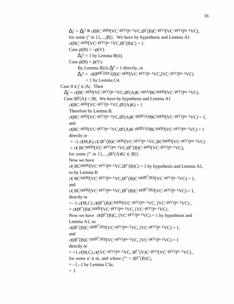
= 1 by Lemma C4.Case 0 ≤ j' ≤ |A|. Then ∆ 'j' = O(BC–ρ(B)[VC–ρ(V)]n–1VC,σj'(A)K–±ρ(A)BC±ρ(B)[VC–ρ(V)]m–1VC). Case |σj'(A)| < |B|. We have by hypothesis and Lemma A1

O(BC–ρ(B)[VC–ρ(V)]n–1VC,σj'(A)K) = 1Therefore by Lemma B,O(BC–ρ(B)[VC–ρ(V)]n–1VC,σj'(A)K+ρ(σj'(A))BC±ρ(B)[VC–ρ(V)]m–1VC) = 1,andO(BC–ρ(B)[VC–ρ(V)]n–1VC,σj'(A)K–ρ(σj'(A))BC±ρ(B)[VC–ρ(V)]m–1VC) = 1directly or = –1.O(M,K).O( σj'''(B)C–ρ(B)[VC–ρ(V)]n–1VC,BC±ρ(B)[VC–ρ(V)]m–1VC) = O( BC±ρ(B)[VC–ρ(V)]m–1VC,σj'''(B)C–ρ(B)[VC–ρ(V)]n–1VC),for some j''' in 1,...,|σj'(A)K| ≤ |B|.Now we haveO( BC±ρ(B)[VC–ρ(V)]m–1VC,σj'''(B)C) = 1 by hypothesis and Lemma A1, so by Lemma BO( BC±ρ(B)[VC–ρ(V)]m–1VC,σj'''(B)C+ρ(σj'''(B))[VC–ρ(V)]n–1VC) = 1,andO( BC±ρ(B)[VC–ρ(V)]m–1VC,σj'''(B)C–ρ(σj'''(B))[VC–ρ(V)]n–1VC) = 1,directly or= –1.O(M,C).O(σj'''(B)C±ρ(B)[VC–ρ(V)]m–1VC, [VC–ρ(V)]n–1VC) ,= O(σj'''(B)C±ρ(B)[VC–ρ(V)]m–1VC, [VC–ρ(V)]n–1VC) .Now we have O(σj'''(B)C, [VC–ρ(V)]n–1VC) = 1 by hypothesis andLemma A1, soO(σj'''(B)C–ρ(σj'''(B))[VC–ρ(V)]m–1VC, [VC–ρ(V)]n–1VC) = 1,andO(σj'''(B)C+ρ(σj'''(B))[VC–ρ(V)]m–1VC, [VC–ρ(V)]n–1VC) = 1directly or= +1.O(M,C).O([VC–ρ(V)]m–1VC, σj''''(V)C–ρ(V)[VC–ρ(V)]n'–1VC) , for some n' ≥ m, and where j'''' = |σj'''(B)C|,= –1.–1 by Lemma C3a,= 1.

17

Case |σj'(A)| = |B|. We haveO(BC,σj'(A)K) = 1 by hypothesis, and soO(BC–ρ(B)[VC–ρ(V)]n–1VC,σj'(A)K) = 1Then by Lemma B(ii)O(BC–ρ(B)[VC–ρ(V)]n–1VC,σj'(A)K+ρ(σj'(A))BC±ρ(B)[VC–ρ(V)]m–1VC)

= 1, andO(BC–ρ(B)[VC–ρ(V)]n–1VC,σj'(A)K–ρ(σj'''(B))BC±ρ(B)[VC–ρ(V)]m–1VC)

= 1 directly or= –O(M,K) O([VC–ρ(V)]n–1VC,BC±ρ(B)[VC–ρ(V)]m–1VC)= O(BC±ρ(B)[VC–ρ(V)]m–1VC,[VC–ρ(V)]n–1VC)

Now O(BC,[VC–ρ(V)]n–1VC) = 1 by hypothesis and Lemma A1, soO(BC–ρ(B)[VC–ρ(V)]m–1VC,[VC–ρ(V)]n–1VC) = 1, andO(BC+ρ(B)[VC–ρ(V)]m–1VC,[VC–ρ(V)]n–1VC) = 1unless BC+ρ(B) = τ|BC|(V), in which caseO(BC+ρ(B)[VC–ρ(V)]m–1VC,[VC–ρ(V)]n–1VC) = O(M,C) O([VC–ρ(V)]m–1VC,σ|BC|(V)C–ρ(V)[VC–ρ(V)]n–2VC) if n>1, = –1.–1 = 1 by Lemma C3a,

or, if n=1, = O(M,C) O([VC–ρ(V)]m–1VC,σ|BC|(V)C) = 1 by hypothesis.

Case |σj'(A)| > |B|. We have by hypothesis and Lemma A1O(BC,σj'(A)K–±ρ(A)BC±ρ(B)[VC–ρ(V)]m–1VC),so by Lemma B∆ = O(BC–ρ(B)[VC–ρ(V)]n–1VC,σj'(A)K–±ρ(A)BC±ρ(B)[VC–ρ(V)]m–1VC)= 1.

That χ(+1,±n)(AK,BC) are maximal is the dual of the statement just proven.

18

III.2 Proof of Theorem 2

III.2.1 Extreme-shift Lemmas

The proof of Theorem 2, to be given shortly, is constructive. It uses a deterministic algorithm

(the Retraction Algorithm; see III.2.4) to effect a decomposition of an extremal word in V# that

reveals its seed of origin. The "retraction" to the seed entails the repeated truncation of the word—

deletion of the extreme shift—and it relies both on the extremality of the word remaining at each

stage of the process, and on knowledge of the extreme shift of the remaining word. The first

lemma in this section identifies the extreme shifts of the extremal words that are specified as

emanations in Theorem 1. Those that follow assure the extremality of the words that remain after

each truncation, and enable us to identify the extreme shifts of those words.

Lemma D: α . For each n in 1,2,..., E+1([L] n–1C) = C and E–1([R]n–1K) = K.

ψ. If (UQ, VQ) is a ψ-seed, then with Ω=–O(M,Q), for each n in 1,2,...,EΩ( ψ±n(UQ,VQ) ) = VQ.

χ . If (AK,BC) is a χ-seed, then for each n in 1,2,...,the greatest shift of β(–1,±1)(AK,BC) is AK,

the greatest shift of χ(–1,±n)(AK,BC) is AK–(±ρ(A))BC,the least shift of β(+1,±1)(AK,BC) is BC, andthe least shift of χ(+1,±n)(AK,BC) is BC±ρ(B)AK.

Lemma E1: a . If UXVC, with X∈B, is in V# and is minimal, and WC is its greatest shift,then UC is minimal.

b . If UXVC, with X∈B, is in V# and maximal, and VC is its least shift,then UK is maximal.

Lemma E2: If UVXVC, with X ∈B, is in V# and minimal with greatest shift VC, then UVCis minimal with greatest shift VC.

Lemma E3: If UYVXUC, with X,Y ∈B, is in V# and minimal with greatest shift VXUC,then UC is the least shift of VXUC.

19

III.2.2 Uniqueness lemma

The Retraction Algorithm (III.2.4) ignores the letter that precedes the extreme shift at each

stage of the decomposition, except the last. The following lemma is needed to show that

knowledge of those letters is nevertheless not lost. The reason is that the extremal words specified

in Theorem 1 are unique in the following senses.

Lemma F: α . [L] nC, is the only word in V # of length |[L]nC| with greatest shift C,n ∈ 0,1,..., and [R]nK, is the only word in V# of length |[R]nK| with leastshift K.

ψ . If (AQ,BQ) is a ψ-seed, the words Ψn±(AQ,BQ) defined in Theorem 1 are theonly words in V# of the form

AX0BX1BX2...BXnBQ, with Xi ∈ Bfor which E–O(M,Q)(AX0BX1BX2...BXnBQ) = BQ.

χ. If (AK,BC) is a χ-seed, thenχ(–1,±n)(AK,BC) , n ∈ 1,2,...,

are the only minimal words in V# of the formW±x = BX0 AK±BX1 AK±BX2 ...AK±BXn–1 AK ±BC

for which E+1(W±x) = AK+ρ(A)BC, andχ(+1,±n)(AK,BC) , n ∈ 1,2,...,

are the only maximal words in V# of the formW±x = AX0 BC±AX1 BC±AX2 ...BC±AXn–1 BC±AK

for which E–1(W±x) = BC–ρ(B)AK.

III.2.3 Seed existence lemmas

The Retraction Algorithm eventually generates a pair of words in V#, (UP,VQ), with

P,Q∈C,K, which is asserted to be the seed from which the original word emanates. The

following lemmas are required to ensure that the pair generated does in fact have the defining

properties of a seed of the appropriate type.

Lemma G1: a . If AXBC in V#, with X∈B, has least shift BC, then O(BC,σj(AK)) = 1 for all j ∈ 0,...,|A|.

20

b . If AXBC in V#, with X∈B, is maximal with least shift BC, then O(σj(BC),AK) = 1 for all j ∈ 0,...,|B|.

Lemma G2: a . If AXBC is in V#, with X∈B, is minimal with greatest shift BC, and A isnot a shift of B, then O(AC,σj(BC)) = 1 for all j ∈ 0,...,|B|.

b . If AXBC is in V#, with X∈B, is minimal with greatest shift BC, and B isnot a shift of A, then O(σj(AC),BC) = 1 for all j ∈ 0,...,|A|.

Lemma H1: If AXBC in V#, with X∈A', is maximal with least shift BC, then (AK,BC) is aχ-seed.

Proof: BC is minimal by hypothesis.AK is maximal by Lemma E1b.O(BC,σj(AK)) = 1 for all j ∈ 0,...,|A| by Lemma G1a.O(σj(BC),AK) = 1 for all j ∈ 0,...,|B| by Lemma G1b.

Lemma H2: If AXBC in V#, with X∈B, is minimal with greatest shift BC, and neither A norB is a shift of the other, then (BC,AC) is a ψ-seed.

Proof: BC is maximal by hypothesis.AC is minimal by Lemma E1a.O(σj(AC),BC) = 1 for all j ∈ 0,...,|A| by Lemma G2b.O(AC,σj(BC)) = 1 for all j ∈ 0,...,|B| by Lemma G2a.

II.2.4 Proof of Theorem 2

We are finally in a position to present a proof of our result that every word in V# emanates

from a unique seed. Given a word in V#, the algorithm given below determines a seed from

which the word emanates, as well as the complete specification of the emanation. The letters X1,

X2,...,Xn of Lemma F are ignored by the algorithm, but by that lemma, those letters are

determined by X0, which is not ignored. Existence of a seed of origin is thus constructively

demonstrated. Using Lemma D, it is easily checked that all the emanations specified in Theorem 1

are correctly decomposed by the algorithm. That is, the A and B words are recovered, the type of

seed is identified, and the type and indices of the emanation are determined correctly. Uniqueness

therefore follows from the fact that if a word emanates from the seed (AP,BQ) and from the seed

21

(A'P',B'Q'), then the algorithm recovers (AP,BQ) and it recovers (A'P',B'Q'). Since the

algorithm is deterministic, (AP,BQ)=(A'P',B'Q').

Retraction Algorithm:

The seed from which a word in V# emanates is determined by applying the following algorithm.

Case: The word is of the form WC.

Case: WC is maximal.

Case: |W|=0.

WC = C is also minimal, and WC = α–1.

Case: |W|≠0.

Define U,V in B*, X in B, by WC=UXVC, where VC is the least shift of WC.

Then by Lemma H1, (UK,VC) is a χ-seed, and

WC = β(+1,ρ(UX))(UK,VC).

Case: WC is minimal.

I. If the greatest shift of WC is C, then WC= α–|WC|, by Lemma Fα.

Otherwise set TC = WC, and VC = E+1(WC) which is maximal.

II. If VC is not a shift of TC go to step III.

Otherwise, define UX, X in B, by TC = UXVC. By Lemma E1, UC is minimal.

By Lemma E2, if VC is a shift of UC, it is its greatest shift. Redefine T by

TC=UC and repeat step II.

III. Let n be the number of times the body of step II was performed.

If TC is a shift of VC, it is its least shift by Lemma E3.

Therefore defining SX, with X in B, by VC = SXTC, (SK,TC) is a

χ-seed by Lemma H1, and WC= χ(–1,–ρ(SX)n)(SK,TC).

Otherwise, neither TC nor VC is a shift of the other, whence by Lemma H2,

(VC,TC) is a ψ-seed, and WC = Ψ–ρ(TX)n(VC,TC).

(Note: TC cannot become empty by removal of VC because TC≠VC since one is

maximal and the other is minimal, and VC is not the one word, C, that is both. That

possibility was disposed of in step I.)

Case: The word is of the form WK.

The seed is determined by the dual under involution of the algorithm above.

22

Examples:

(i) We apply the algorithm to the word LLMMMC, which is minimal.

I. Set TC = LLMMMC, and VC = MC the greatest shift.

II. VC is a shift of TC, so set UX = LLMM, and redefine TC = UC = LLMC.

VC is a shift of TC, so set UX = LL, and redefine TC = UC = LC.

VC is not a shift of TC, so proceed to step III.

III. Now VC = MC, TC = LC, X=L, n=2, and ρ(TX) = ρ(LL) = +1.

TC is not a shift of VC, therefore LLMMMC = Ψ–2(MC,LC).

(ii) We apply the algorithm to the word LMC, which is minimal.

I. Set TC = LMC, and VC = MC the greatest shift.

II. VC is a shift of TC, so set UX = L, and redefine TC = UC = C.

VC=MC is not a shift of TC=C, so proceed to step III.

III. Now VC = MC, TC = C, X=L, n=1, and ρ(TX) = ρ(L) = +1.

TC is a shift of VC, so set SX by MC = SXTC, that is S=1 and X=M,

and so LMC = χ(–1,–1)(K,C).

IV. A new partial order on finite kneading sequences

Theorems 1 and 2 yield directly a new partial order on finite kneading sequences that we

formalize as follows:

- say K1 is a strict parent of K2 if K2 emanates from a seed of the form (K0,K1)or (K1,K0), (by

Theorem 2, each finite kneading sequences has exactly two strict parents),

- say K1 is a parent of K2 , in symbols K1«K2, if K1 is a strict parent of K2, or K1 = K2.

- say K1 is an ancestor of Kn , in symbols K1««Kn, if there exists a sequence (K1,K2,...Kn),

with n≥2, such that Ki«Ki+1 for 1 ≤ i ≤ n–1.

Defining the topological entropy h(K) of a kneading sequence K as the infimum of topological

entropies of maps f such that K is a kneading sequence of f, we have:

23

Theorem 3: K1««K2 ⇒ h(K1) ≤ h(K2).

The two-parameter family of stunted saw-tooth maps are defined in the next section. Since

the kneading data of a map determines its topological entropy[MT], and since any kneading data

for +-+-bimodal maps is realized by some stunted sawtooth map, we can also define the

topological entropy h(K) of a kneading sequence K as the infimum of topological entropies of

stunted saw-tooth maps Ta,b+ such that K is a kneading sequence of Ta,b

+ . The proof of Theorem 3

will be given in the next section, using this alternate but equivalent definition of h(K).

V. Stunted saw-tooth maps

We set define the full +-+-bimodal stunted saw-tooth map S+ as:

S+ =

5x if 0 ≤ x ≤ 15

,

5 (35

- x) if 25

≤ x ≤ 35

,

5 ( x - 45

) if 45

≤ x ≤ 1 ,

1 if 15

≤ x ≤ 25

,

0 if 35

≤ x ≤ 45

.

(The symbol S– will be reserved for the analogous -+--bimodal map, treated elsewhere[R].)

The graph of S+ is a succession of a hill and a valley. It is easy to check that the set of itineraries

for this map is the set of all possible itineraries for +-+-bimodal maps. We can now define a

two-parameter family of +-+-bimodal stunted saw-tooth maps Ta,b+ by setting

min ( S+(x), a ) under the hill,Ta

+,b(x) =

max ( S+(x), 1–b ) in the valley.

For the map Ta,b+ to be an endomorphism of the unit interval imposes the constraints

0 ≤ a ≤ 1, 0 ≤ b ≤ 1, a+b ≥ 1. (*)

24

The set of parameter values (a,b) satisfying (*) is denoted by P+. Figure 1.0 shows the graph of

S+ and the parameter space P+. All kneading sequences of the truncated maps Ta,b+ can be

understood as the itineraries under S+ of those points which are closer to one of the turning points

than any other point in their orbit. This makes the study of these maps quite simple: the arguments

presented in [GT] and [BMT] for stunted maps in the unimodal case extend easily; in particular,

any +-+ kneading data occurs for some pair (a,b). More on general stunted families will be

reported in [DGMT]; here we use these maps for the sake of illustration and to provide a geometric

picture to display the results of Theorems 2 and 3.

In P+, following [MaT1-MaT3], [M] and [RS1, RS2] we define subsets corresponding to

finite kneading sequences, which can be described as follows (proofs are straightforward and left

to the reader):

- Any finite maximal kneading sequence terminating K is realised on a single segment of straight

line parallel to the a-axis, with one external end point on the line b=1, and one end point called

internal in the interior of P+ or on the boundary a+b=1: this segment is called a K-ligament.

- Any finite minimal kneading sequence terminating C is realised on a single segment of straight

line parallel to the b-axis, with one external end point on the line a=1, and one end point called

internal in the interior of P+ or on the boundary a+b=1: this segment is callet a C-ligament; we say

ligament for either K-ligament or C-ligament.

- For any n>1 and a permutation s on n elements obtainable by restricting a +-+ bimodal map to

one of its periodic orbits, the bone Bs is the set of pairs (a,b) such that for Ta,b+ , one of the turning

points belongs to a periodic orbit where the restriction of Ta,b+ acts like s. Any bone is made of

two connected curves BsC and Bs

K where the superscript indicates which turning point belongs to

the periodic orbit. The curves BsC and Bs

K intersect at two points, one of which is a χ-point, the

other one corresponding to the coexistence of two periodic orbits with the same s, each of which

contains a turning point. The curve BsC has two segments parallel to the a-axis, each havingwith

one external end point on the line b=1. The interior end points of these segments are joined by a

piece of K-ligament which belongs to BsC. The curve Bs

K has two segments parallel to the b-axis,

25

each havingwith one external end point on the line a=1. The interior end points of these segments

are joined by a piece of C-ligament which belongs to BsK .

Figures 1.1, 1.2 and 1.3 represent (not to scale) respectively α, χ and ψ points, the

ligaments which cross at these points, and the ligaments and pieces of bones so generated in P+.

These figures give a geometrical interpretation of Lemma D and of Theorems 1 and 2. Since some

attention was paid in [MaT1-MaT3] to the relations of a bone Bs to the two bones corresponding to

periodic orbits obtained from those in Bs by a period doubling bifurcation, Figure 1.4 shows how

such triples of bones fit in the emanation discussion. In these figures, heavy black lines

correspond to bones or to the lines a=1 and b=1, light black lines correspond to ligaments. The

grey region in Figure 1.2 is the domain where the periodic orbit with maximal itinerary

(AK ρ(A)BC–ρ(B))∞ and minimal itinerary (BC–ρ(B)AK ρ(A))∞ is an attractor. To simplify the

annotation of the figures, we write WQ+ for WQρ(W) and WQ– for WQ–ρ(W). In Figures 1.1, 1.2

and 1.3, if the grey lines are contracted to points (without creating further crossings on the black

lines) one gets singular simplices which are embeded in the plane as would conjecturally be the

corresponding sets of bones and ligaments for a two parameter family of cubic maps (see

[DGMT]). In Figure 1.1, only the interior of the segment a+b=1 should be contracted to a point;

in all cases, the contraction should take place without affecting the underlying bone. Figures 2.1-

2.4 are counterparts respectively to Figures 1.1-1.4, obtained numerically from the cubic family

given by fa,b(x)=x3–ax+b. Figure 0 showed for this family the region of its parameter space that

corresponds most closely with P+: in the region shown in that figure, the maps are all bimodal

except at the α-seed (a=b=0), and there is an invariant interval containing both critical points.

Proof of Theorem 3:

Maximal kneading sequences are monotonously increasing with a, for fixed b, and with b,

for fixed a. Similarly, minimal kneading sequences are monotonously decreasing with a, for fixed

b, and with b, for fixed a. Consequently, the topological entropy of Ta,b+ increases when any of

the parameters increases, the other parameter being fixed. Hence, the topological entropy on a

ligament is minimal at its internal endpoint. On a bone Bs=BsC∪Bs

K, the topological entropy of Ta,b+

26

is minimal at the corners of BsC and Bs

K which are closest to the line a+b=1. Since up to a finite

number of periodic orbits, the periodic orbit structure of Ta,b+ is unchanged on the ligament part of

each bone (they correspond to lines in a hyperbolic region in the polynomial case), the topological

entropy is unchanged there, and can only change by increasing when following a non-ligament part

parallel to either the a-axis or the b-axis. This shows that at α, χ and ψ points, the topological

entropy is not greater than on the lines emanating there, which is what we had to prove.

Combining Theorems 2 and 3 with the elementary properties of the bones and ligaments in

P+ yields the following result:

Theorem 4: In P+, any two seeds can be joined by finite path made of pieces from finitely many

bones and ligaments.

27

References

[B] P.L. Boyland,"Bifurcations of circle maps: Arnol'd tongues, bistability and rotation

intervals," Commun. Math. Phys. 106 (1986) 353-381.

[DGMT] S.P. Dawson, R. Galeeva, J. Milnor and C. Tresser, to appear.

[D] R.L. Devaney, "Genealogy of periodic points of maps of the interval," Trans. AMS

265, (1981) 137-146.

[FK] S. Fraser and R. Kapral, "Universal vector scaling in one-dimensional maps", Phys.

Rev. A 30 (1984) 1017-1025.

[GT] J.M. Gambaudo and C. Tresser,"A monotonicity property in one dimensional

dynamics," Cont. Math. 135 (1992) 213-222.

[MaT1] R.S. Mackay and C. Tresser, "Transition to topological chaos for circle maps,"

Physica 19D (1986) 206-237.

[MaT2] R.S. Mackay and C. Tresser, "Some flesh on the skeleton: the bifurcation structure of

bimodal maps," Physica 27D (1987) 412-422.

[MaT3] R.S Mackay and C. Tresser,"Boundary of topological chaos for bimodal maps of the

interval," J. London Math. Soc. 37 (1988), 164-81.

[Mi1] J. Milnor, "Remarks on iterated cubic maps," Experimental Math. 1 (1992), 5-24.

[MT] J. Milnor and W. Thurston, "On iterated maps of the interval," Springer Lecture Notes

1342 (1988), 465-563.

[M] P. Mumbrù and I. Rodriguez, "Estructura, periòdica i entropia topològica de les

applications bimodals," Doctoral Thesis, Universidad Autùnoma de Barcelona (1987).

[BG] R. Perez and L. Glass, "", Phys. Rev. Lett. 48 (1982) 1772-XXXX.

[R] J. Ringland, to appear.

[RS1] J. Ringland and M. Schell, "The Farey tree embodied—in bimodal maps of the

interval," Phys. Lett. A 136 (1989) 379-386.

[RS2] J. Ringland and M. Schell, "Genealogy and bifurcation skeleton for cycles of the

iterated two-extremum map of the interval," SIAM J. Math. Anal. 22 (1989) 1354-

1371.

28

[STZ] R. Siegel, C. Tresser and G. Zettler, "A decoding problem in dynamics and in number

theory," Chaos 2 (1992) 473-493.

[TW] C. Tresser and R.F. Williams, "Splitting words and Lorenz braids," Physica D 62

(1993) 15-21.

See also W.-Z. Zeng and L. Glass, "Symbolic dynamics and skeletons of circle maps", Physica

D 40, 218-234 (1989).

29

Figure Captions

Figure 0 Loci of some finite kneading sequences for a two-parameter cubic family.

Figure 1.0 Graph and parameter space of the stunted sawtooth family, Ta,b+ .

Figure 1.1 The α-seed in the family Ta,b+ .

Figure 1.2 A χ-seed in the family Ta,b+ .

Figure 1.3 Two ψ-seeds in the family Ta,b+ .

Figure 1.4 Period-doubling in the family Ta,b+ .

Figure 2.1 The α-seed in the cubic family fa,b.

Figure 2.2 A χ-seed in the family fa,b.

Figure 2.3 Two ψ-seeds in the family fa,b.

Figure 2.4 Period-doubling in the family fa,b.