A Functional-Structural Plant Model--Theories and Its

Applications in Agronomy

MengZhen Kang 1, Paul-Henry Cournède

2, Amélie Mathieu

2, Véronique Letort

2, Rui Qi

1,2,

ZhiGang Zhan3

(1: LIAMA, Institute of Automation, Chinese Academy of Sciences, 100080, Beijing, China)

(2: Laboratory of Applied Mathematics, Ecole Centrale Paris, 92295 France)

(3: College of Resources and Environmental Sciences, China Agricultural University, 100094, Beijing, China)

Abstract: Functional-structural plant models (FSPM) simulate plant development and growth,

usually accompanied with visualization of the plant 3D architecture. GreenLab is a generic and

mechanistic FSPM: various botanical architectures can be produced by its organogenesis model,

the growth rate is computed from leaf area, and the biomass partitioning is governed by the sink

strength of growing individual organs present in plant structure. A distinguished feature of

GreenLab model is that, the plant organogenesis (in terms of the number of organs) and growth (in

terms of organ biomass) are formulated using dynamic equations, aside simulation software. This

facilitates analytical study of model behaviour, bug-proof of simulation software, and application of

efficient optimization algorithm for parameter identification and optimal control problems.

Currently several levels of GreenLab model exist: (1) the deterministic one (GL1): plants have a

fixed rule for development without feedback from the plant growth; (2) the stochastic level (GL2):

pant development is probabilistic because of bud activities, which has influence on plant growth; (3)

the feedback model (GL3): the plant development is dependent on the dynamic relationship

between biomass demand and supply (and in turn the environment).

This paper presents the typical GreenLab theories and applications in past ten years: (1) calibration

of GL1 for getting sink and source functions of maize; (2) features of GL2 and its application on

wheat plant; (3) rebuilt of the rhythmic pattern of cucumber using GL3; (4) optimization of model

parameters for yield improvement, such as wood quantity (for trees); (5) the possible introduction

of genetic information in the model through detection of quantitative trait loci for the model

parameters; (6) simulation of plant competition for light.

Keywords: GreenLab, FSPM, GL1, GL2, GL3, plant optimization, QTL, plant competition

1 Introduction

In past years, Functional-Structural Plant Models (FSPMs) were attracting interest from plant

modellers (Vos et al 2007). GreenLab methodology, began to develop around ten years ago, have

been applied for several different kinds of crops, including maize (Guo et al 2006, Ma et al 2007,

Ma et al 2008), tomato (Dong et al 2008), chrysanthemum (Kang et al 2006), pine tree (Guo et al

2007), arabidopsis (Letort et al 2007), and wheat (Kang et al 2008). Other undergoing

GreenLab-based application for various purposes includes modelling on beech tree, rice, cotton,

cucumber, sweet pepper, etc. On the other hand, theoretical work on GreenLab went on in parallel,

includes the formalism of the organogenesis model (de Reffye et al 2003), structure factorization of

complex plant structure for fast computation (Cournède et al 2006), analytical computation of mean

and variance of stochastic model (Kang et al 2007), generation of rhythmic pattern of branch or

fruits from GreenLab dynamic system (Mathieu et al 2007), link between GreenLab parameters and

QTL (Letort et al 2008), computation of inter-plant competition (Cournède et al 2008). Software

based on GreenLab model has been developed for simulation and parameter identification,

including CornerFit (for single-stem plants), GreenScilab (open-source and generic), and

DigiPlante (generic and efficient). In this paper, we review the general form of GreenLab model,

present its different levels, and its applications on real plants. Three theoretical works are presented

to show future possible applications.

2 General presentation

A time step (a growth cycle, GC) in GreenLab model corresponds to the temperature sum it takes to

generate a growth unit (GU), being a metamer for crops or an annual axis for trees. The plant

development is simulated using automaton (Zhao et al 2001). All organs (leaf blade and petiole,

internode pith, layer, female and male organs, root system) are sinks that share biomass from a

common pool. The sink strength of an organ can vary with time. The biomass of each organ is a

result of biomass competition in each GC. From its biomass, the size of each organ is computed.

Beside the seed that provide biomass in initial GCs, leaf is the main source organ. The production

of a plant is a function of green leaf area.

The number of GC since the appearance of an organ or a branch is called chronological age (CA).

Another property of organs or buds/branches is physiological age (PA). PA is expressed in integer

values too, being one for main stem. Branches are physiologically older than its parent axis, except

the case of reiteration. The tip of an axis can mute into another physiological age. The maximum

PA in plant is noted as Pm. Organs of the same CA and PA are supposed to have the same sink

strength and thus the same biomass (except for internodes that can have secondary growth). Based

on the notion PA, using substructure decomposition (Cournède et al 2006), the number of organs in

each GC can be computed with equations without resorting to simulation.

A highly compact form of GreenLab model can be expressed as in Eqn. 1:

),,(

),,(

Ef

Tf

gO

dO

PNQ

QPN

=

= (1)

In Eqn. 1, No are the number of new organs of each CA and PA in plant structure at each growth

cycle, O=B (blade), S (sheath), pith (P), layer (L), female (F), male (M), or root (R). Pd is the

vector of development parameters that define the plant topology, including the number and PA of

leaves, buds, flowers and axillary buds in each kind of GU, the repetition times of GU in an axis

before mutate into another PA, etc. T is the air temperature. In the model, the development speed of

the plant, or number of days per GC, is mainly decided by the air temperature. Q include the

biomass of ay part of plant at each growth cycle: those of individual organs, a certain type of

organs (say fruits), or the whole plant. E is the environmental data. Pg is the vector of growth

parameters that control the biomass production and partitioning among organs, includes:

(1) the relative sink strength of organs (POp), p being PA of organs. That of blade in main stem is set

to one as the reference, i.e. PB1=1;

(2) parameters of sink variation function (φOi) that describe the change of sink strength of

individual organs, i being CA of organs. The actual sink strength of an organ of PA p and CA i is

thus POpφO

i;

(3) the empirical parameters of source function ( β and γ in Eqn. 3);

(4) the functioning duration (tf) and expansion duration (tx) of organs;

(5) internode allometric parameters and specific leaf weight (e).

The total demand for biomass of plant at GC n is computed as sum of sink strength of all growing

organs, as in Eqn. 2:

∑∑∑= =

+−=O

P

p

t

i

i

O

p

O

inp

On

ox

PNDm

1 1

1, ϕ (2)

NOp,n-i+1

is number of organ O of PA p and CA i at plant age n. A commonly used biomass

production function of GreenLab is inspired by the Beer-Lambert law of light extinction:

))exp(1( nnn SEQ γβ −−= (3)

Where β, γ are empirical model parameters estimated by model inversion, Sn is the total green leaf

area of the plant at growth cycle n.

The biomass increment of an organ is a function of biomass supply and demand:

n

ni

O

p

O

ip

nOD

QPq 1,

,−=∆ ϕ (4)

The biomass of an organ is the sum of increment since its appearance:

∑∑= +−

−

=+−

=∆=i

j jn

jnj

O

p

O

i

j

jp

jno

ip

nOD

QPqq

1 11

,

1,

,

, ϕ (5)

From Eqn. 5, it can be seen that the biomass of an organ depends on the ratio (Q/D) during its life

span. Although organs of the same type and PA have the same sink strength in the model, their final

biomasses are not necessary the same if they appear at different moments. In this sense, the organ

architecture records the growth history of the plant.

3 Three Levels of the GreenLab model and their applications

Different levels of GreenLab model have been developed, namely GL1, GL2, and GL3. Among

them, GL1, the deterministic level, is the common part. An important issue of model application is

parameter identification. Part of the parameters can be observed directly, such as specific leaf

weight, internode allometric parameter, development parameters (case of deterministic model),

functioning and expansion time of organs. Organ sink strength, sink expansion functions, and

empirical parameters for biomass production, are difficult to measure directly. These (hidden)

parameters can be estimated using optimization algorithms aiming at minimizing the model output

and measured data. Below we present the parameterizing in GL1, and extra features in GL2 and

GL3.

3.1 GL1 and parameter identification for maize

GL1, the basic version, has been applied to simulate many plants: maize (Ma et al 2007), pine tree

(Guo et al 2006), arbidobisis (Letort et al 2008), chrysanthemum (Kang et al 2006), etc. In GL1,

the plant development (and consequently the number of organs) is not influenced by the biomass

supply, but follows a fixed rules. The form of GL1 is thus differs from Eqn. 1:

),,(

),(

Ef

Tf

gO

dO

PNQ

PN

=

= (6)

In the case that the plant is of single stem structure, the numbers of organs are easy to compute, and

one can concentrate on the identification of sink-source parameters. For field plants, the plant

growth rate Qn, and organ growth rate ∆qo,n are internal and transient variables, which are

technically difficult to be directly measured. Therefore, the source and sink functions cannot be

separately determined by using classical fitting methods. On the other hand, the plant architecture

and organ biomass are accumulative results of the dynamical processes since the plant emergence,

including plant growth and organ development. From the modeling point of view, since GreenLab

model output variables (number, size and mass of organs) implicitly and nonlinearly depend on the

hidden parameters in the recursive simulation process, these parameters can be identified through

inverse modeling, i.e., the parameter values are determined by minimizing the differences between

observed and simulated data. When this is achieved, GreenLab model can fit best to plant

morphological and architectural data observed at several points of time. There are several different

optimization algorithms available to minimize the proposed objective function, for example, the

Levenberg-Marquardt method, genetic algorithms, or stochastic methods. The

Levenberg-Marquardt method is practically proved more efficient than the others in terms of

computation time.

For maize, under moderate density, the final structure of the maize plant consists of four types of

organs: the main stem, the leaf sheathes and blades, a tassel (the male organ) at top, and one or

several ears (the female organs) set at different nodal positions along the stalk. For maize, the

variation of sink strength of individual organs was taken as the form of Eqn. 7:

MF,I,S,B,},1|max{

5.01

5.0where

0

1/

11

=≤≤=

−−

−=

>

≤≤=

−−

Otig

t

i

t

ig

ti

tig

Ox

i

OO

xOxO

i

O

Ox

OxO

i

Oi

O

OO

µ

µϕ

βα

(7)

There are 12 parameters to be estimated for maize plants, including two empirical parameters of the

source function (β and γ in Eqn. 3), and ten parameters of the sink functions (PO in Eqn. 2 and αO

in Eqn. 7, o = B, S, I, F, M, denoting leaf blade, sheath, internode, ear and tassel, respectively, αO

+βO ≡ 5 for all organs).

During the course of plant development and growth, plants were regularly sampled and measured

in detail, including size (length, diameter, area) and fresh or dry mass of each organ. The data were

stored in a specified structure according to the position, type and attribute of organs. From these

data the target was constructed for the model to fit. In order to get an estimate of the source and

sink parameters, we use the weighted least-square criterion:

))(())(()( θZWθZθ FF T −−=φ (8)

where Z is the target vector consisting of measurement data on plant samples at several stages; θθθθ is

the parameter vector to be estimated, a subset of Pg; F(θθθθ) is a vector function (i.e., the recursive

simulation equations) with respect to θθθθ, whose components are simulated data corresponding to Z;

W is a positive definite matrix which weights the various observations.

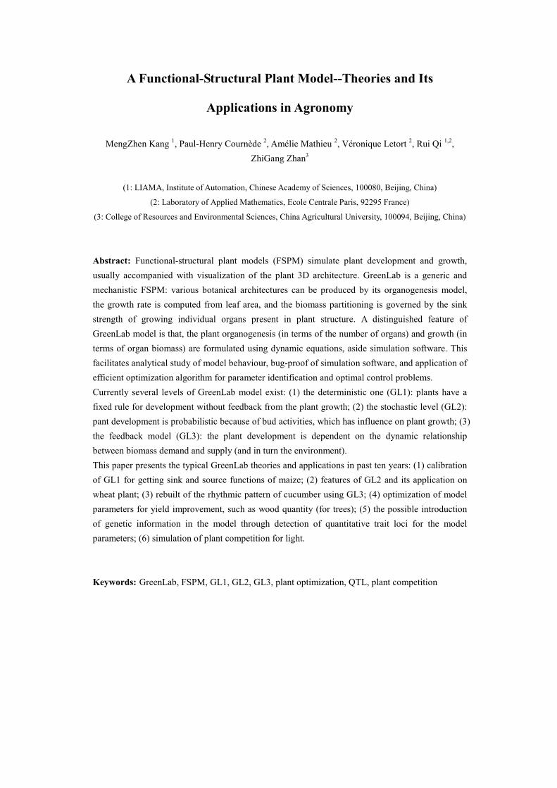
GL1 model were fitted to three stages of maize plants. The fitting results are shown in Fig. 1. Based

on the calibrated parameters, the model was tested against independent data from different years

(Ma et al 2007) and different population densities (Ma et al 2008).

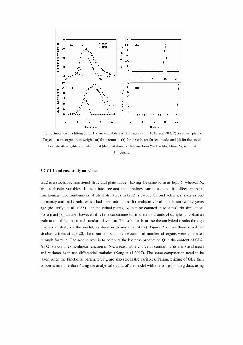
Fig. 1. Simultaneous fitting of GL1 to measured data at three ages (i.e., 10, 18, and 30 GC) for maize plants.

Target data are organ fresh weights (a) for internode, (b) for the cob, (c) for leaf blade, and (d) for the tassel.

Leaf sheath weights were also fitted (data not shown). Data are from YunTao Ma, China Agricultural

University.

3.2 GL2 and case study on wheat

GL2 is a stochastic functional-structural plant model, having the same form as Eqn. 6, whereas No

are stochastic variables. It take into account the topology variations and its effect on plant

functioning. The randomness of plant structures in GL2 is caused by bud activities, such as bud

dormancy and bud death, which had been introduced for realistic visual simulation twenty years

ago (de Reffye et al. 1988). For individual plants, NO can be counted in Monte-Carlo simulation.

For a plant population, however, it is time consuming to simulate thousands of samples to obtain an

estimation of the mean and standard deviation. The solution is to use the analytical results through

theoretical study on the model, as done in (Kang et al 2007). Figure 2 shows three simulated

stochastic trees at age 20; the mean and standard deviation of number of organs were computed

through formula. The second step is to compute the biomass production Q in the context of GL2.

As Q is a complex nonlinear function of NO, a reasonable choice of computing its analytical mean

and variance is to use differential statistics (Kang et al 2007). The same computation need to be

taken when the functional parameter, Pg, are also stochastic variables. Parameterizing of GL2 then

concerns no more than fitting the analytical output of the model with the corresponding data, using

the methods as for GL1.

Fig.2. Stochastic tree simulated using a single set of functional and developmental parameters. Analytical

mean and standard deviation of number of phytomers are 15120.1 and 3765.8 respectively.

GL2 feature is interesting for plants that show strong randomness in topology. First try of

application was on wheat plant. Through introducing tiller bud outgrowth probability and tiller

survival probability, the number of phytomers in tillers and the final remaining tillers were well

fitted, as shown in Fig. 3. This prepared the second step of model calibration concerns fitting on

biomass production. The average plant, instead of individual plants, is fitted, representing the

common plant among those of various topologies.

Plant age (cycle)

0 2 4 6 8

Mean of number of phytomers

0

5

10

15

20

PA 1

PA 2

PA 3

PA 1 Fit

PA 2 Fit

PA 3 Fit

(a) (b)

Fig.3. The number of phytomers and remaining ears in main stem (PA 1), primary tillers (PA 2), secondary

tillers (PA 3) of a wheat plant, with population density 100 plants m-2 (data from CWE group, Wageningen

University).

3 GL3 and sweet pepper

GL3 is a feedback version, having the same form as Eqn. 1 regarding the biomass production but

the topological events of the plant are assumed to be controlled by the ratio of biomass (Q; Eqn. 3)

to demand (D; Eqn. 2), that is to say that the numbers of the different type of organs NO are

computed as functions of this ratio. It allows reproducing the plant phenotypic plasticity as the

number of organs depending on the plant vigour.

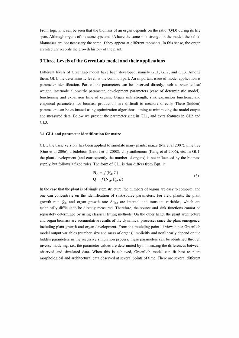
As an example, this GL3 model can be used to simulate the cyclic patterns of fruits that have been

observed in the sweet pepper plant (Marcelis et al 2004) or in the cucumber plant (Marcelis, 1992).

Fruit abortion can occur within the first days after fruit anthesis. In the GL3 model, we assume that

if the ratio of biomass to demand (Q/D) is under a given threshold a few growth cycles after the

fruit appearance, then the one will abort. Otherwise it will continue growing. This model was

calibrated on pruned cucumber plants where the fruit growth is not limited by fruit initiation

(Mathieu et al 2008). Fig. 4 shows the differences between the plant measurements and the model

simulation. Fruits appeared on the plant when the ratio of biomass to demand exceeds a threshold

(Fig. 5) which explains the two waves of fruits on the stem. The cyclic patterns of fruits are

explained as a consequence of the assimilate competition between organs.

(a) (b)

(c) (d)

Fig. 4. Simulation and measurement for a cucumber plant at three different ages (9GC, 15 GC, 31 GC). We

used a multifitting procedure with the same set of source-sink parameters. The variations in the phytomer

profile along the stem are a consequence of the competition between sinks.

(a) (b)

Fig. 5. Ratio of biomass production to demand as a function of growth cycles and corresponding plant.

Horizontal line represents threshold value (a). When the ratio exceeds this value, fruits grow on the main stem.

Two timeframes in which fruit set can take place are observed (b).

4 Theoretical study

The virtual plant itself as described by GreenLab model is a complex dynamic system. As it can

behave close to real plants through model calibration, it is meaningful to do virtual experiment on

GreenLab plants. The theoretical studies present here are experiments done in computer. These

works may pioneer the future applications.

4.1 Possible link with Quantitative Trait Loci (QTL)

In maize (Ma et al 2007) and tomato (Dong et al 2007), although the relative sink strength (of pith

and fruit) vary, their expansion function remain the same for plants grown under different

population densities. Consequently, it can be hypothesized that some of GreenLab parameters are

species-specific and gene-based. Let Y denote the vector of these ‘genetic’ parameters. Introducing

genetics in the model allows simulating plant reproduction and studying the evolution in time of a

virtual population without requiring to time- and space- consuming experiments. In our model, the

genotype of the plant is defined as a set of two vectors C1 and C2, representing the chromosomes

(for sake of simplicity, only pairs of chromosomes are considered, although maize is generally

haploid). The components of these vectors (alleles) are positive real numbers representing the

parameter variation around a reference value Yref. An application f defines the rules of allele

expression (dominance or additivity) and then the ‘genetic’ vector of GreenLab parameters Y is

calculated as a product of matrices:

Y = C × A × f (C1, C2) (9)

A is a matrix defining the influence of genes on each parameter, including pleiotropic rules (one

gene has an influence on several parameters) or combinations of several gene effects on one

parameter. C is a diagonal matrix introduced to ensure that the coefficients of Y are of the same

order range (similar to barycentre calculation). Reproduction between two plants is simulated with

realistic rules (Poisson law) driving the probability of crossing-over occurrences, see Letort et al.

(2007) for details. It allows generating a virtual mapping population (recombinant inbred lines) to

simulate the procedure of quantitative trait loci (QTL) detection, as done by geneticists on real

plants (de Vienne 2003). Their goal is to localize the chromosomal segments (called QTL) that

contain genes of interest (influencing the yield, for instance). In our model, QTL detection is

analogous to determination of the coefficients of matrix A that drives the link between the plant

genotype and the model parameters. Results shown in Fig. 6 are consistent with the opinion

defended in several recent papers that underlined the potential benefits of introducing physiological

knowledge into breeding programs (e.g. Chapman et al 2003; Hammer et al 2006; Tardieu et al

2003; Yin et al 2003). Our study illustrated that QTL detection on model parameters is more

accurate on model parameters than on the classical morphological data such as cob weight (Fig. 5).

We conclude that this method is worthy to be tested on real plant populations. GreenLab

parameters provide new criteria to renew the breeding process and to characterize model-based

ideoptypes.

=

...

4

3

2

1

Y

Y

Y

YEnvironment

LOD score for

parameter 1

(Blade Resistance)

LOD score for

parameter 2

(Sink of sheath)

LOD score for cob

weight

AllelesAEndogenous

parameters

GreenLab

0 0 1 0 0 0 0 1 0 0 0 0 0 0 0

0 0 0 3 0 0 0 0 2 0 0 0 0 1 0

0 0 1 0 0 0 0 0 0 0 1 1 0 0 0

0 1 0 1 0 3 0 0 0 0 3 1 1 0 0

1 0 0 1 1 1 0 1 0 1 1 0 1 1 1

…

⋅

...

8.0

7.0

1

95.0

⋅D=

...

4

3

2

1

Y

Y

Y

YEnvironment

LOD score for

parameter 1

(Blade Resistance)

LOD score for

parameter 2

(Sink of sheath)

LOD score for cob

weight

AllelesAEndogenous

parameters

GreenLab

0 0 1 0 0 0 0 1 0 0 0 0 0 0 0

0 0 0 3 0 0 0 0 2 0 0 0 0 1 0

0 0 1 0 0 0 0 0 0 0 1 1 0 0 0

0 1 0 1 0 3 0 0 0 0 3 1 1 0 0

1 0 0 1 1 1 0 1 0 1 1 0 1 1 1

…

⋅

...

8.0

7.0

1

95.0

⋅D

0 0 1 0 0 0 0 1 0 0 0 0 0 0 0

0 0 0 3 0 0 0 0 2 0 0 0 0 1 0

0 0 1 0 0 0 0 0 0 0 1 1 0 0 0

0 1 0 1 0 3 0 0 0 0 3 1 1 0 0

1 0 0 1 1 1 0 1 0 1 1 0 1 1 1

…

⋅

...

8.0

7.0

1

95.0

⋅D

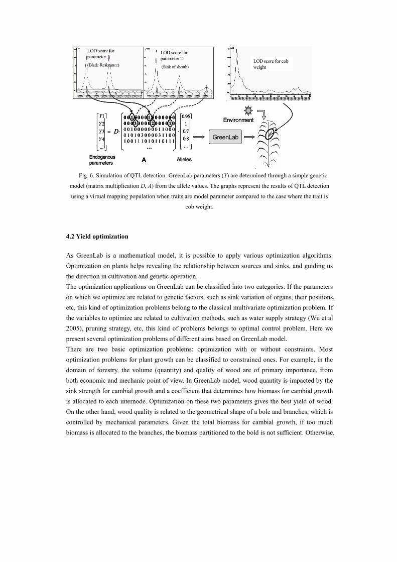
Fig. 6. Simulation of QTL detection: GreenLab parameters (Y) are determined through a simple genetic

model (matrix multiplication D, A) from the allele values. The graphs represent the results of QTL detection

using a virtual mapping population when traits are model parameter compared to the case where the trait is

cob weight.

4.2 Yield optimization

As GreenLab is a mathematical model, it is possible to apply various optimization algorithms.

Optimization on plants helps revealing the relationship between sources and sinks, and guiding us

the direction in cultivation and genetic operation.

The optimization applications on GreenLab can be classified into two categories. If the parameters

on which we optimize are related to genetic factors, such as sink variation of organs, their positions,

etc, this kind of optimization problems belong to the classical multivariate optimization problem. If

the variables to optimize are related to cultivation methods, such as water supply strategy (Wu et al

2005), pruning strategy, etc, this kind of problems belongs to optimal control problem. Here we

present several optimization problems of different aims based on GreenLab model.

There are two basic optimization problems: optimization with or without constraints. Most

optimization problems for plant growth can be classified to constrained ones. For example, in the

domain of forestry, the volume (quantity) and quality of wood are of primary importance, from

both economic and mechanic point of view. In GreenLab model, wood quantity is impacted by the

sink strength for cambial growth and a coefficient that determines how biomass for cambial growth

is allocated to each internode. Optimization on these two parameters gives the best yield of wood.

On the other hand, wood quality is related to the geometrical shape of a bole and branches, which is

controlled by mechanical parameters. Given the total biomass for cambial growth, if too much

biomass is allocated to the branches, the biomass partitioned to the bold is not sufficient. Otherwise,

if allocation is too much for the bole, the load of the bole will be too heavy and fall down easily,

see Fig. 7. As a result, besides maximizing the bole weight, the angle of the bold at the top is

limited under a threshold. The optimization problem on wood quantity and quality for a tree is the

classical optimization problem with constraints.

(a) (b)

Fig. 7. 3D illustration of wood quality and quantity, for a 40 years old virtual tree. (a) trunk weight

5.04E+4g (b) trunk weight 2.45E+5g.

Pruning is a common cultivation action in agriculture or forestry, in order to make plants growing

better and to get better yield. For example, most of side branches of tomatoes are removed to make

sure fruit yield. Obviously the behavior of plant is modified if pruning is done during plant growth.

A special case is to prune leaves, such as tea plant. Here leaf plays double roles: it is not only the

source organs the provide biomass to whole plant, but also the yield. For this problem, we add a

control variable that represents the proportion of number of leaves pruned among the living leaves.

With the objective being maximizing pruned leaves, it is an optimal control problem. An ongoing

optimization issue concerns the relationship among palm tree, insects and parasites. In this system,

leaves produce biomass through photosynthesis, insects eat leaves and parasites suppress the

population growth of insects. The optimization problem is complex because of interaction among

the three actors. It is necessary to study the population growth of insects and parasites, both affect

significantly the growth behaviour of the palm tree. In addition, to avoid destroying leaves,

pesticide is used. Considering the fact that pesticide kills not only insect adults but also parasite

adults, and the price of pesticide is very expensive, in order to reduce the cost and increase its use

efficiency (kill only insect adults), it is important to decide when pesticide is put to palm tree. This

is again an optimal control problem.

4.3 Plant competition

GreenLab is an individual-based plant growth model. However, for applications in agriculture and

forestry, it has to be extended to the scale of plant population. For this purpose, inter-plant

competition for light is taken into accounted, see Cournède et al (2008).

For high density crops at full cover, the model should be equivalent to the classical equation of

field crop production. For example, Howell and Musick (1985) showed that biomass production is

proportional to crop transpiration T. It is driven by the potential evapotranspiration, the soil water

content and the exposed green leaf surface area, evaluated using Beer-Lambert’s extinction law. If

at cycle n, En denotes the product of the potential evapotranspiration modulated by a function of the

soil water content, k is the Beer-Lambert extinction coefficient related to leaf angular deviation and

LAIn is the leaf area index, Tn is estimated as:

( )( )nnn LAIkET −−= exp1 (10)

Finally, the biomass production per unit surface area Qnc is:

( )( )nnn

c

n LAIkETQ −−== exp1µµ (11)

where µ is the Water Use Efficiency. From the individual plant production equation of GreenLab

( Eqn. 3) and in the case of a homogeneous crop of density d , the biomass production per unit

surface area is directly deduced:

( )( )nnn

c SdEQ ηβ −−= exp1 (12)

Let Sd=1/d. For a homogeneous crop, LAIn =Sn/Sd, by identifying (11) and (12), the empirical

parameters β and η are thus given by β=µSd and η=µ/Sd. This analogy helps us derive a general

formulation for the individual plant production equation:

( ) ( ) ( )( )( )pp /exp1 SnSkSnEnQ −−= µ (13)

Sp is a reference surface, such that Sp=Sd in the case of homogeneous high density crops (see the

application to maize for different densities in Ma et al 2008). In the case of spatially heterogeneous

crops (like rapeseed fields), a Voronoi tessellation can help determine the Sp of all individuals in the

population. For tree communities, things can get far more complex. First, the reference surface can

not be taken as a constant: it increases along plant growth. Cournède et al. (2008) proposed to

model it as a function of the leaf surface: Sp(n)=Sp0(Sn/Sp

0)

τ. Simulation results are shown in Fig. 8,

which shows the impact of density on tree architecture. Moreover, a generalized Poisson model of

leaf repartition inside the canopy was proposed by Cournède and de Reffye (2007) to compute

plant production for individuals in heterogeneous and potentially multi-specific tree stands.

Although the simulation results are encouraging, this model still lacks field validation.

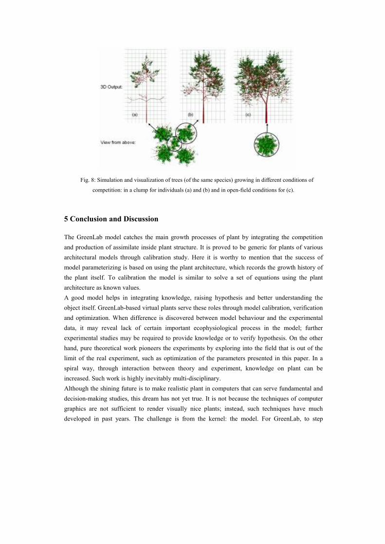
Fig. 8: Simulation and visualization of trees (of the same species) growing in different conditions of

competition: in a clump for individuals (a) and (b) and in open-field conditions for (c).

5 Conclusion and Discussion

The GreenLab model catches the main growth processes of plant by integrating the competition

and production of assimilate inside plant structure. It is proved to be generic for plants of various

architectural models through calibration study. Here it is worthy to mention that the success of

model parameterizing is based on using the plant architecture, which records the growth history of

the plant itself. To calibration the model is similar to solve a set of equations using the plant

architecture as known values.

A good model helps in integrating knowledge, raising hypothesis and better understanding the

object itself. GreenLab-based virtual plants serve these roles through model calibration, verification

and optimization. When difference is discovered between model behaviour and the experimental

data, it may reveal lack of certain important ecophysiological process in the model; further

experimental studies may be required to provide knowledge or to verify hypothesis. On the other

hand, pure theoretical work pioneers the experiments by exploring into the field that is out of the

limit of the real experiment, such as optimization of the parameters presented in this paper. In a

spiral way, through interaction between theory and experiment, knowledge on plant can be

increased. Such work is highly inevitably multi-disciplinary.

Although the shining future is to make realistic plant in computers that can serve fundamental and

decision-making studies, this dream has not yet true. It is not because the techniques of computer

graphics are not sufficient to render visually nice plants; instead, such techniques have much

developed in past years. The challenge is from the kernel: the model. For GreenLab, to step

forward this goal, the direction is the combination of GL2 and GL3, leading to a stochastic

functional-structural plant model with interaction (GL4). The demand of this new generation has

come already from plants in study, including sweet pepper, wheat, cucumber, etc.

In GreenLab, there are still several parameters that lack explicit physiological meanings. To stand

on sound basis, it is necessary to link them with actual measurable values, to make it easier to

compare the parameters of plants under different condition, or different species. Linkage between

GreenLab and traditional process-based models is also worthy to be made to benefit each other.

Acknowledgement

Special thanks to the father of GreenLab, Dr. Philippe de Reffye. Thanks to Dr. Ma YunTao

from China Agricultural University who provided data of maize. The work is supported in part

by Natural Science Foundation of China (#60703043), Chinese 863 program

(#2008AA10Z218 and # 2006AA10Z229).

Reference

1. Chapman S, Cooper M, Podlich D, Hammer G (2003) Evaluating plant breeding strategies by simulating gene action

and dryland environment effects. Agron J 95: 99–113

2. Cournède PH, Kang MZ, Mathieu A, et al (2006) Structural factorization of plants to compute their functional and

structural growth. Simul 82: 427–438

3. Cournède PH, de Reffye P (2007) A generalized Poisson model to estimate inter-plant competition for light. In:

Fourcaud T, Zhang XP (eds) proc PMA06 - Plant growth model, simul, vis and their appl. IEEE Computer Society,

Los Alamitos, California: 11-15

4. Cournède PH, Mathieu A, Barthélémy D, et al (2008) Computing competition for light in the GreenLab model of

plant growth: a contribution to the study of the effects of density on resource acquisition and architectural

development. Ann Bot 101: 1207-1219

5. Dong QX, Louarn G, Wang YM et al (2008) Does the structure–function model GREENLAB deal with crop

phenotypic plasticity induced by plant spacing? A case study on tomato. Ann Bot 101:1195-1206

6. Guo Y, Ma YT, Zhan ZG, et al (2006) Parameter optimization and field validation of the functional-structural model

GreenLab for maize. Ann Bot 97: 217–230

7. Hammer G, Cooper M, Tardieu F, et al (2006) Models for navigating biological complexity in breeding improved crop

plants. Trends Plant Sci 11: 587–593

8. Guo H, Letort V, Hong LX, et al (2007) Adaptation of the GreenLab model for analyzing sink-source relationships in

Chinese Pine saplings. In: Fourcaud T, Zhang XP (eds) proc PMA06 - Plant growth model, simul, vis and their appl.

IEEE Computer Society, Los Alamitos, California: 236-243

9. Kang MZ, Heuvelink E, de Reffye P (2006) Building virtual chrysanthemum based on sink-source relationships:

preliminary results. Acta Hortic 718: 129–136

10. Kang MZ, Cournède PH, de Reffye P, et al (2007) Analytic study of a stochastic plant growth model: application to

the GreenLab model. Mat Comput Simul 78: 57-75

11. Kang MZ, Evers JB, Vos J, et al (2008) The derivation of sink functions of wheat organs using the GreenLab model.

Ann Bot 101: 1099-1108

12. Letort V, Cournède PH, Lecoeur J, et al (2007) Effect of topological and phenological changes on biomass

partitioning in Arabidopsis thaliana inflorescence: a preliminary model-based study. In: Fourcaud T, Zhang XP (eds)

proc PMA06 - Plant growth model, simul, vis and their appl. IEEE Computer Society, Los Alamitos, California:

65-69

13. Letort V, Mahe P, Cournède PH, et al (2008) Quantitative genetics and functional-structural plant growth models:

simulation of quantitative trait loci detection for model parameters and application to potential yield optimization.

Ann Bot 101: 1243-1254

14. Ma YT, Li BG, Zhan ZG, et al (2007) Parameter stability of the functional-structural plant model GREENLAB as

affected by variation within populations, among seasons and among Growth Stages. Ann Bot 99: 61-73

15. Ma YT, Wen M, Guo Y, et al (2008) Parameter optimization and field validation of the functional structural model

GreenLab for maize at different population densities. Ann Bot 101: 1185-1194

16. Marcelis LFM (1992) The dynamics of growth and dry matter distribution in cucumber. Ann Bot 69: 487-492

17. Marcelis LFM, Heuvelink E, Baan Hofman-Eijer LR, et al (2004) Flower and fruit abortion in sweet pepper in

relation to source and sink strength. J Exp Bot 55: 2261-2268

18. Mathieu A, Cournède PH, Barthélémy D, et al (2007) Conditions for the generation of rhythms in a discrete dynamic

system. Case of a functional structural plant growth model. In: Fourcaud T, Zhang XP (eds) proc PMA06 - Plant

growth model, simul, vis and their appl. IEEE Computer Society, Los Alamitos, California: 26-33

19. Mathieu A, Cournède PH, Barthélémy D, et al (2008) Rhythms and alternating patterns in plants as emergent

properties of a model of interactions between development and functioning. Ann Bot 101: 1233-1242

20. de Reffye P, Edelin C, Francon J, et al (1988) Plant models faithful to botanical structure and development.

Computer Graphics 22: 151-158

21. de Reffye P, Goursat M, Quadrat J, et al (2003) The dynamic equations of the tree morphogenesis GreenLab model.

Research Report, INRIA-Rocquencourt, no RR-4877

22. Tardieu F (2003) Virtual plants: modelling as a tool for the genomics of tolerance to water deficit. Trends Plant Sci 8:

9-14

23. de Vienne D ( 2003) Les marqueurs moléculaires en génétique et biotechnologies végétales. INRA Editions

24. Vos J, Marcelis LFM, de Visser PHB, et al (ed) (2007) Functional–structural plant modelling in crop production.

Springer, Dordrecht

25. Wu L, Le Dimet FX, Hu BG, et al (2005) A water supply optimization problem for plant growth based on GreenLab

model. ARIMA J: 194-207

26. Yin X, Stam P, Kropff MJ, et al (2003) Crop modeling, QTL mapping, and their complementary role in plant breeding.

Agron J 95: 90–98

27. Zhao X, de Reffye P, Xiong FL, et al (2001) Dual-scale automaton model of virtual plant growth. Chin J Comput 24:

608–615