A Framework for Fault Diagnosis inManaged Pressure Drilling Applied to

Flow-Loop Data

Anders Willersrud ∗ Lars Imsland ∗ Alexey Pavlov ∗∗Glenn-Ole Kaasa ∗∗

∗Department of Engineering Cybernetics, Norwegian University ofScience and Technology, N-7491 Trondheim, Norway(email: [anders.willersrud, lars.imsland]@itk.ntnu.no).

∗∗Department of Intelligent Drilling, Statoil Research Centre,N-3905 Porsgrunn, Norway (email: [alepav, gkaa]@statoil.com).

Abstract: Data from a medium-scale horizontal flow loop test facility is used to test faultdiagnosis in managed pressure drilling. The faults are downhole incidents such as formationinflux, fluid loss, drillstring washout, pack-off, and plugging of the drill bit, which are importantto detect and handle in order to avoid downtime and possibly dangerous situations. In thispaper a fault diagnosis scheme based on an adaptive observer and the generalized likelihoodratio test is applied on the experimental data. The different types of faults are detected andtheir location are isolated using friction parameter estimates. Results indicate that the methodcan in most cases identify the type of fault, whereas the location is sometimes more uncertain.

Keywords: Fault diagnosis, managed pressure drilling, flow loop, nonlinear adaptive observer

1. INTRODUCTION

Drilling for oil and gas is always associated with risk. Asreservoirs become depleted or more difficult to reach, oper-ations become more complex, and safety margins smaller.It will then be increasingly important to improve monitor-ing and control of the downhole drilling process to avoidincidents and reduce downtime. In drilling the pressurein the well must be carefully monitored and controlledto be above the formation pore pressure and below itsfracture pressure. If the pressure is lower than the porepressure, formation fluids can start flowing into the well.If the pressure becomes too high, the formation can startto fracture leading to losses of drilling fluid (“mud”) tothe formation, damaging the reservoir. Managed pressuredrilling (MPD) is a method which seals off the annulusaround the drillstring and routes the return flow of thedrilling fluid through a controlled choke, making it possi-ble to more carefully control the downhole pressure. SeeFig. 1 for a schematic overview. With this technology it ispossible to drill wells with narrow pressure margins. In thiscase, detection and handling abnormal situation becomesvery important.A situation which is critical to detect is an influx ofreservoir fluids, also known as a kick. An influx can happenif some parts of the wellbore become underbalanced, i.e.,with well pressure below formation pore pressure. If gasenters the annulus, the hydrostatic pressure will decreasedue to lower mixed density. This can in turn increase theinflux, making the situation worse. If continued uncon-trolled, the situation can develop into a blowout, whichis an uncontrolled flow of reservoir fluids into the welland must be prevented at all costs. One of the causes

Fig. 1. Managed pressure drilling with possible faults.Measurements are labeled in blue, actuators in green.

for the well to become underbalanced is lost circulationof drilling fluid. If enough fluid is lost, the back-pressureis lost which will decrease the hydrostatic head in theannulus. Poor transport or accumulation of cuttings canresult in formation of a pack-off, which in turn changesthe annular friction and can also result in a stuck pipe.Moreover, lost circulation of drilling fluid is important

from a cost perspective since the drilling fluid can containexpensive chemicals. In addition to being a safety risk, thementioned incidents will increase the nonproductive timeduring drilling, which on average is 20-25 % of the drillingtime and thus a major cost (Godhavn, 2010).In this paper, data from a medium-scale flow loop isused to study contingency and fault diagnosis in managedpressure drilling. The test setup is made to mimic a realdrilling process as closely as possible, and manages toreproduce many of the possible faults in a realistic manner.The faults we study are illustrated in Fig. 1, which allcause changes in pressure. Some faults are also related tochanges of mass flow through the system, such as influxand lost circulation. In addition to topside pressure mea-surements, distributed pressure sensors is used along thedrill pipe. This is a rather new communication technologycalled wired drill pipe, which increases the number ofmeasurement points as well as data bandwidth (Nygaardet al., 2008). These measurements are used in an adaptiveobserver to estimate friction parameters throughout thesystem. Applying a detection algorithm on the estimatedfriction parameters, it is possible to detect and isolate thedifferent faults causing changes to friction and flow. Theposition is isolated to be in between two pressure sensors.This is done without using a flow meter downstream thechoke.Detection of influx and loss is studied in Hauge et al.(2013), where also the position is estimated. Reitsma(2010) considers the stand pipe and choke pressures fordetection of influx and loss, but does not isolate theposition. He argues that it is beneficial to have faultdiagnosis without a coriolis flow meter downstream thechoke, due to intolerance to gas flow, limited space, andvibrations offshore. In Gravdal and Lorentzen (2010),wired drill pipe is used to detect and isolate a kick inbetween pressure sensors.This study is based on the methods developed in Willer-srud and Imsland (2013), using an adaptive observer ap-proach for fault diagnosis. The model and the adaptiveobserver used are briefly presented in Sec. 2. The methodsfor fault diagnosis are presented in Sec. 3, using statisticalmethods to detect changes in estimated parameters. Somedetails about the flow loop are presented in in Sec. 4, andthe fault diagnosis framework is demonstrated in Sec. 5showing the main results. The results are discussed inSec. 6 and the paper is summarized in Sec. 7.

2. DRILLING MODEL AND OBSERVER

The model of the drilling system used in this study is asimplified hydraulics model (Kaasa et al., 2012) with twocontrol volumes, one for the drillstring and one for theannulus, connected through the drill bit. See Fig. 1 fora schematic overview. The model is represented by theordinary differential equationsdppdt

= βdVd

(qp − qbit) (1a)

dpcdt

= βaVa

(qbit + qbpp − qc) (1b)

dqbit

dt= 1M

(pp − pc − F (θ, qbit)− (ρa − ρd)ghTVD) (1c)

where pp is the drilling pump pressure, pc is the chokepressure, and qbit the flow through the bit. The parameterβ is the bulk modulus, V is the volume, and ρ is the densityin the control volume. Subscripts d and a denote thedrillstring and annulus control volumes, respectively. Theconstant g is the gravitational acceleration. The parameterM is the integrated density over the cross section A, givingan integrated value over the segment ∆Li = Li − Li−1 as

Mi =∫ Li

Li−1

ρi(x)Ai(x)dx.

The total integrated value from the the pump to the chokeis M = Md + Ma. Furthermore, the true vertical depthhTVD is assumed known.The choke flow can be represented by the choke equation

qc = θcCvg(uc)√pc − pc,0

where Cv is the choke constant, uc is the choke opening,and pc,0 is pressure downstream the choke. The choke char-acteristics g(uc) is found experimentally. The parameter θcrepresents possible choke plugging, and is nominally equalto 1. The total friction F (θ, qbit) is given by

F (θ, qbit) = (θd + θb + θa1 + θa2 + θa3 + θa4)q2bit (2)

which is the sum of friction in the drillstring, bit, andannular sections between pressure measurements, respec-tively. This friction model is best matched when thereis turbulent flow of a Newtonian fluid. The vector ofunknown parameters is

θ = [θd, θb, θa1, θa2, θa3, θa4, θc]> . (3)The relationship between the wired drill pipe pressuremeasurements and the annular friction is given by

pbit,0 = pp − θdq2bit +Gd(ρd) (4a)

pbit = pbit,0 − θbq2bit (4b)

p1 = pc + θa1q2bit +G1(ρa) (4c)

p2 = p1 + θa2q2bit +G2(ρa) (4d)

p3 = p2 + θa3q2bit +G3(ρa) (4e)

pbit = p3 + θa4q2bit +G4(ρa) (4f)

where Gi(ρa) = ρag(hi−1 − hi), i ∈ 1, . . . , 4 is the hydro-static pressure difference between the two measurementpoints in the annulus, and Gd = ρdghTVD is the hydro-static pressure in the drillstring. It is assumed that hi isknown.Note that in Willersrud and Imsland (2013) the formationof a pack-off giving unknown annular friction parameterswas studied, but where it was assumed that the bit anddrillstring parameters were known. In this paper thereare possible faults such as bit plugging and drillstringwashout, making it necessary to also have unknown bitand drillstring parameters.The adaptive observer in Willersrud and Imsland (2013),which is based on Besancon (2000), is used to estimatestates and parameters. The system above can be writtenon the form

x = α(x, z, u) + β(x, z, u)θ (5a)z = η(x, z, u) + λ(x, z, u)θ (5b)

where x(t) ∈ Rn are the states, z(t) ∈ Rm are ad-ditional measurements, u(t) ∈ Rp are the inputs, θ ∈Rq are unknown parameters we want to estimate, and

α(·), β(·), η(·) and λ(·) are locally Lipschitz. Specifically,x = [pp, pc, qbit]>, z = [ pbit,0, pbit, p1, p2, p3, pbit]>,u = [qp, qbpp, uc]>, and with system matrices

α(x, u) =

−βdVd

(x3 − u1)βaVa

(x3 + u2)1M

(x1 − x2 − (ρa − ρd)ghTVD)

(6a)

η(x, z) = [x1 +Gd, z1, x2 +G1, . . . (6b)z3 +G2, z4 +G3, z5 +G4]> (6c)

β(x, u) = [β3 β3 β3 β3 β3 β3 β2] (6d)λ(x) = [λ1 λ2 λ3 λ4 λ5 λ6 0] (6e)

where β2 = βa

Va

[0,−Cvg(u3)

√x2 − pc,0, 0

]>,β3 = 1

M

[0, 0,−x2

3]>, λ1 = λ2 = −x2

3ej , and λ3 = λ4 =λ5 = λ6 = x2

3ej , where ej is the jth column of the identitymatrix I6 ∈ R6×6.Theorem 1. Given an observer for system (5) on the form

˙x = α(x, z, u) + β(x, z, u)θ −Kx(x− x) (7a)˙θ = −Γβ>(x, z, u)(x− x)− Λλ>(x, z, u)(z − z) (7b)z = η(x, z, u) + λ(x, z, u)θ (7c)

where Kx,Λ,Γ > 0 are tuning matrices, and assume θ = 0.Let ex = x − x and eθ = θ − θ be variables for the errordynamics, where e = [e>x , e>θ ]> = 0 is an equilibrium point.Then e = 0 is globally exponentially stable if

Γ−1Λλ>(·)λ(·)− β>(·)K>Kβ(·) > kIq (8)for some constant k > 0, where Iq ∈ Rq×q is the identitymatrix, and K = 1

2(In −K−1

x

).

See Willersrud and Imsland (2013) for proof of Thm. 1.Note that the assumption θ = 0 is made to facilitate inthe convergence proof of the observer. In reality there arefaults and measurement noise, making θ stochastic.

3. FAULT DIAGNOSIS

Fault diagnosis is a term which typically describes methodsfor detecting a fault, isolating its location, and identifyingthe type of fault. Common for fault diagnosis methodsis that they rely on some residual sensitive to faults andpreferably insensitive to disturbances and modeling un-certainties (Blanke et al., 2006; Ding, 2008). The residualis typically designed to give zero value at the fault-freenormal case, and a nonzero value during a fault. Ding(2008) describes two strategies to evaluate the residual.One of them is norm based evaluation using robust controltheory. Another one is statistic testing using statisticalmethods, which is used in this paper.By estimating friction parameters throughout the systemit is possible to differentiate between pressure losses due tochange in flow from change in friction. If we then classifysets of parameter changes it is possible to identify thekind of fault, and to some extent its location. The frictionparameters can be estimated by an adaptive observer,such as the one described in Sec. 2. In order to haveresiduals sensitive to parameter changes with zero value

for the nominal case and nonzero for a faulty case, a changedetection algorithm is employed.

3.1 Change detection algorithms

The data used in this paper is quite noisy, and thusa statistical evaluation of the estimated parameters (3)is used to detect changes. These methods assume someknown probability distribution pθ(y) of a random variabley with known parameter θ = θ0 for the fault-free case H0and some known or unknown parameter θ1 for the faultcase H1. If θ1 is known, the cumulative sum (CUSUM)type of algorithms can be used, if not the generalizedlikelihood ratio (GLR) is typically applied. An excellentoverview of these algorithms is given in Basseville andNikiforov (1993).A change between the two hypotheses

H0 : θ(i) = θ0 for 1 ≤ i ≤ kH1 : θ(i) = θ0 for 1 ≤ i ≤ k0 and

θ(i) = θ1 for k0 ≤ i ≤ kat time k0 is detected if a decision function g(k) increasesabove a threshold h, namely

if g(k) ≤ h accept H0,

if g(k) > h accept H1.

The log-likelihood between the known and unknown pa-rameter is an expression for the probability of y havingeither parameter value θ0 or θ1 and is given by

Skj (θ1) =k∑i=j

ln pθ1(y(i))pθ0(y(i)) (9)

where k is the current sample time (Blanke et al., 2006).With both change time k0 and parameter θ1 unknown theGLR decision function is given by

g(k) = maxk−N+1≤j≤k

maxθ1

Skj (θ1), (10)

where we use a window of size N of the data series. If pθ(y)is Gaussian and the variance known, the decision functionis given by

g(k) = 12σ2 max

k−N+1≤j≤k

1k− j+ 1

k∑i=j

(y(i)− µ0)

2

(11)

which we will assume for the parameters in this paper. Inaddition, we will use sgn(g(k)) = sgn(µ0−µ1) to determinein which direction the parameter is moving. An underlyingassumption is that Gaussian parameter estimates is areasonable approximation.

3.2 Fault isolation and identification

In the previous section it was discussed how to detect achange in a parameter. A change due to a fault is called asymptom (Isermann, 2006; Ding, 2008). Since the differentfaults generate different symptoms, it may be possible toisolate and identify an occuring fault. In Tab. 1 the faultsare listed with the corresponding changes in parameters.The naming used for the faults is done in the same wayas for the parameters, where fault i is a fault happeningbetween sensor pi−1 and pi. As an example, ‘fluid loss4’ is a loss of fluids between sensors p3 and p4 in the

annulus. Following Isermann (2006); Blanke et al. (2006),we see that all faults can be uniquely identified based onthe symptoms, but that two or more faults may not beidentified correctly simultaneously. It is not possible to,e.g., detect fluid loss and drillstring washout simultane-ously. This is not necessary a weakness in practice, sincedownhole faults such as the ones described in this paperare all quite severe, requiring some counter-measures to betaken. By using the GLR decision function (11) on each of

Table 1. Fault symptoms with increasing (+),decreasing (−) and unchanged (0) behavior.

θd θb θa4 θa3 θa2 θa1 θc

Fluid loss 1 0 0 0 0 0 − +Fluid loss 2 0 0 0 0 − − +Fluid loss 3 0 0 0 − − − +Fluid loss 4 0 0 − − − − +Drillstring washout 1 − − − − − − 0Drillstring washout 2 − − − − − 0 0Drillstring washout 3 − − − − 0 0 0Drillstring washout 4 − − − 0 0 0 0Gas influx 1 0 0 0 0 0 + −Gas influx 2 0 0 0 0 + + −Gas influx 3 0 0 0 + + + −Gas influx 4 0 0 + + + + −Bit plugging 0 + 0 0 0 0 0Choke plugging 0 0 0 0 0 0 −

the parameters in Tab. 1 with a threshold vector h ∈ Rq,all faults can possibly be detected, isolated and identified.Note that this matrix only shows faults that are tested inthe experimental setup, whereas it can easily be extendedto diagnose faults such as pack-off and hole enlargement.

4. MEDIUM-SCALE FLOW LOOP

The experimental setup is a horizontal water-based flowloop of 1400 meters, designed to match a real drilling rigas closely as possible. It is developed by Statoil and setup at the International Research Institute of Stavangerin Norway. Parts of the loop is shown in Fig. 2. Pipesand equipment are full-size with a high rate conventionalpiston rig pump, 5 1/2”-7” outer diameter pipes, andtwo parallel MPD chokes. The setup can emulate faultssuch as gas influx, drillstring washout, loss of circulation,bit plugging, and choke plugging, see Fig. 1. In additionto topside measurements there are distributed pressuresensors, giving the same information as with wired drillpipe. The physical parameters for the flow loop used inthe hydraulic drilling model (1) is given in Tab. 2.

Table 2. Parameters in the hydraulic model.βd,a 22 000 bar Effective bulk modulusρd,a 1.0 kg/L Drilling fluid densityMa 0.374 bar s2/L Integrated density per cross sectionMd 0.581 bar s2/L Integrated density per cross sectionVa 13.2 × 103 L Volume of fluid in annulusVd 8.56 × 103 L Volume of fluid in drillstring

hTVD 2.14 m True vertical depth of bitLd, La 703 m Length of drillstring/annulus

There are some aspects in a real drilling process the flowloop cannot capture. Since the pipes are horizontal, gaspercolating up the annulus will not expand due to de-creased hydrostatic pressure. Furthermore, since the loopconsists of circular pipes, annular effects and drillstringrotation will not be captured.

Fig. 2. Flow loop with drillstring washout and gas injection(left), and fluid loss and drill bit (right).

During analysis of the data a noticeable deadband problemis found in the chokes. This can also be a problem on areal rig using an MPD control system. The servo motorangle is measured, not the actual choke opening. It willthus be a possible discrepancy between logged and actualopening which will affect the estimated choke parameterθc. The data is therefore filtered such that when the chokeopening is going from opening to closing action, or viceversa, it must first travel the deadband distance beforethe opening position actually changes. Another issue in thetest facility is bias on the pressure measurements, whichalso can occur on a real rig (Godhavn, 2010). This must behandled in order to get correct parameter estimates. Anauto-calibration is applied on the pressure sensors whenthere is no flow, since then the pressure drop is onlydependent on known hydrostatic pressure.

5. DIAGNOSIS OF EXPERIMENTAL DATA

The fault diagnosis framework in Sec. 3 is applied toa series of data sets containing the faults bit plugging,drillstring washout between sensors p1 and p2, fluid lossbetween sensors p3 and p4, and finally gas influx betweensensors p1 and p2. These faults are named ‘bit plugging’,‘washout 2’, ‘loss 4’, and ‘gas 2’, respectively. The time ofthe actual faults occurring are shown in the lower panelin Fig. 4. Note that this information is not known in thefault diagnosis.

State and parameter estimation. The observer is initial-ized with x(0) = [10, 20, 10]> and θi(0) = 0, and appliedon the series of data sets which has a sample rate of10 Hz. The observer gains used are Kx = diag{5, 5, 5},Γ = 5× 10−4 × diag{1, 1, 1, 1, 1, 102} and Λ = 5× 10−4 ×diag{1, 1, 1, 1, 1, 102}, where ‘diag’ denotes a diagonal ma-trix. Tuning of observer gains are done primarily to getcorrect scaling. Results for the state estimation is shownin Fig. 3. Since topside pressures are measured, pressureestimation shown in the upper panel is very good asexpected. Note that we measure the pump flow qp and notthe bit flow, shown in the lower panel, and that the bitflow estimate closely follows the measured pump flow. Ifthe flow through restrictions such as the bit or the chokeis different from what the model expects, there will bea change in estimates of θb or θc. This is used in thefault diagnosis framework, where, e.g., θc increases whenthere is a fluid loss. Parameter estimation is shown in

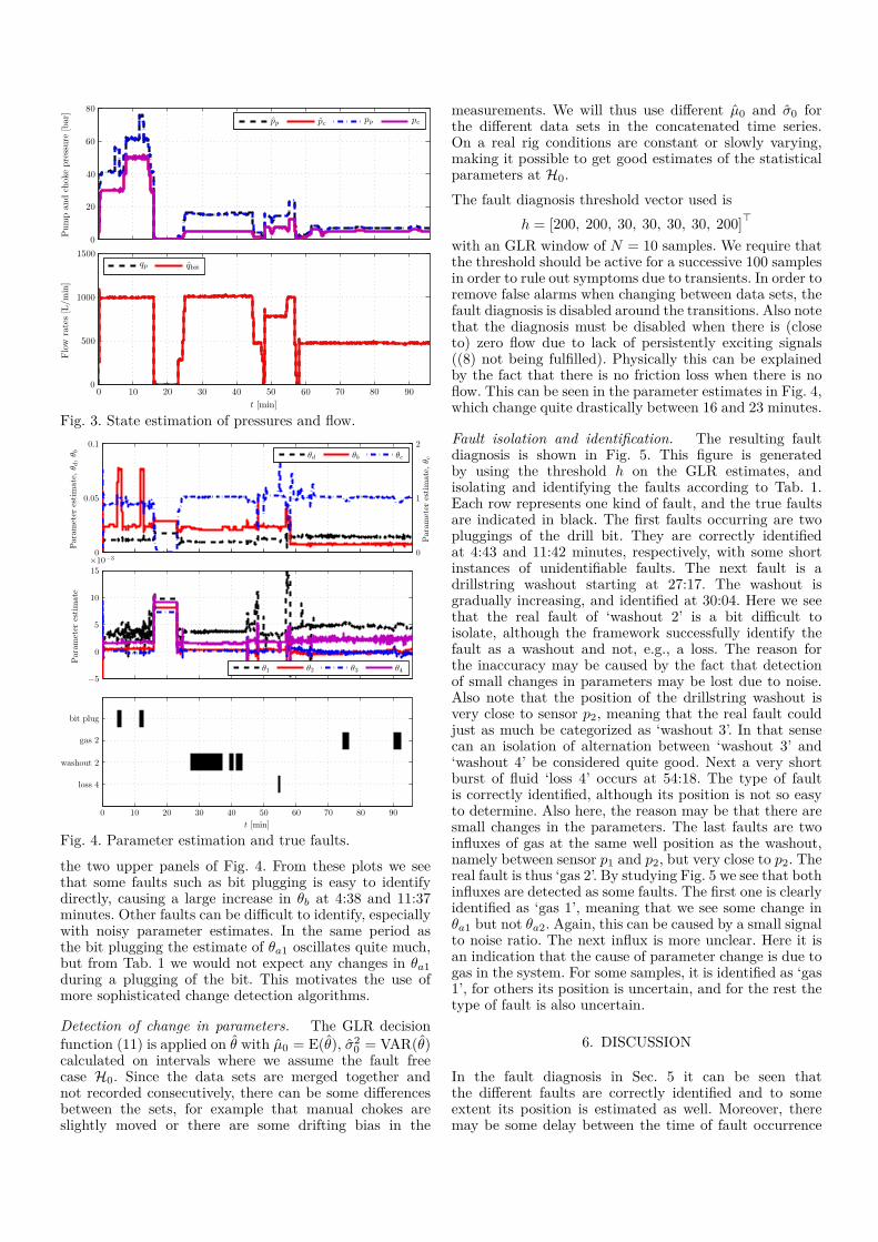
Fig. 3. State estimation of pressures and flow.

Fig. 4. Parameter estimation and true faults.

the two upper panels of Fig. 4. From these plots we seethat some faults such as bit plugging is easy to identifydirectly, causing a large increase in θb at 4:38 and 11:37minutes. Other faults can be difficult to identify, especiallywith noisy parameter estimates. In the same period asthe bit plugging the estimate of θa1 oscillates quite much,but from Tab. 1 we would not expect any changes in θa1during a plugging of the bit. This motivates the use ofmore sophisticated change detection algorithms.

Detection of change in parameters. The GLR decisionfunction (11) is applied on θ with µ0 = E(θ), σ2

0 = VAR(θ)calculated on intervals where we assume the fault freecase H0. Since the data sets are merged together andnot recorded consecutively, there can be some differencesbetween the sets, for example that manual chokes areslightly moved or there are some drifting bias in the

measurements. We will thus use different µ0 and σ0 forthe different data sets in the concatenated time series.On a real rig conditions are constant or slowly varying,making it possible to get good estimates of the statisticalparameters at H0.The fault diagnosis threshold vector used is

h = [200, 200, 30, 30, 30, 30, 200]>

with an GLR window of N = 10 samples. We require thatthe threshold should be active for a successive 100 samplesin order to rule out symptoms due to transients. In order toremove false alarms when changing between data sets, thefault diagnosis is disabled around the transitions. Also notethat the diagnosis must be disabled when there is (closeto) zero flow due to lack of persistently exciting signals((8) not being fulfilled). Physically this can be explainedby the fact that there is no friction loss when there is noflow. This can be seen in the parameter estimates in Fig. 4,which change quite drastically between 16 and 23 minutes.

Fault isolation and identification. The resulting faultdiagnosis is shown in Fig. 5. This figure is generatedby using the threshold h on the GLR estimates, andisolating and identifying the faults according to Tab. 1.Each row represents one kind of fault, and the true faultsare indicated in black. The first faults occurring are twopluggings of the drill bit. They are correctly identifiedat 4:43 and 11:42 minutes, respectively, with some shortinstances of unidentifiable faults. The next fault is adrillstring washout starting at 27:17. The washout isgradually increasing, and identified at 30:04. Here we seethat the real fault of ‘washout 2’ is a bit difficult toisolate, although the framework successfully identify thefault as a washout and not, e.g., a loss. The reason forthe inaccuracy may be caused by the fact that detectionof small changes in parameters may be lost due to noise.Also note that the position of the drillstring washout isvery close to sensor p2, meaning that the real fault couldjust as much be categorized as ‘washout 3’. In that sensecan an isolation of alternation between ‘washout 3’ and‘washout 4’ be considered quite good. Next a very shortburst of fluid ‘loss 4’ occurs at 54:18. The type of faultis correctly identified, although its position is not so easyto determine. Also here, the reason may be that there aresmall changes in the parameters. The last faults are twoinfluxes of gas at the same well position as the washout,namely between sensor p1 and p2, but very close to p2. Thereal fault is thus ‘gas 2’. By studying Fig. 5 we see that bothinfluxes are detected as some faults. The first one is clearlyidentified as ‘gas 1’, meaning that we see some change inθa1 but not θa2. Again, this can be caused by a small signalto noise ratio. The next influx is more unclear. Here it isan indication that the cause of parameter change is due togas in the system. For some samples, it is identified as ‘gas1’, for others its position is uncertain, and for the rest thetype of fault is also uncertain.

6. DISCUSSION

In the fault diagnosis in Sec. 5 it can be seen thatthe different faults are correctly identified and to someextent its position is estimated as well. Moreover, theremay be some delay between the time of fault occurrence

Fig. 5. Fault identification: Bit plugging, drillstring washout, fluid loss and gas kick. True faults are indicated in black.

and detection. One of the reasons is that the method inthis paper is somewhat sensitive to parameter estimation,where a good estimate of the fault free case H0 is required.If the parameter estimation has much noise, changes willnot be detected. Hence will there be a tuning trade-offbetween false and missed fault detection.The fault diagnosis framework in this paper is tested in aflow loop with full-size equipment such as rig pump andchokes, as well as long pipes with typical diameters. It isthus believed that the method could be applied on a realrig with managed pressure drilling installed. A significantdifference is that a real rig will have a true vertical depthof up to several thousand meters. This will change theconditions during a gas influx drastically. If the drillingfluid is oil based and not water based, gas can be dissolvedin the fluid at high pressure and liberated as it comes tolower depth. In addition will cuttings and non-Newtoniandrilling fluid change the friction behavior. These aspectswill have to be taken into consideration in a fault diagnosissystem for a real rig.

7. CONCLUSION AND FUTURE WORK

A novel framework is proposed for fault detection, isolationand identification of downhole faults in managed pressuredrilling. The framework is based on a simple and easyconfigurable hydraulic process model, a nonlinear adaptiveobserver, and threshold tests of generalized likelihood ratiofunctions. One of the challenges is to detect small changeswhen there are noisy signals. The method requires thatwe know when we are in a fault-free scenario, but it isnot limited to knowing the magnitude of the faults. Weapply the framework to data from a medium-scale flowloop and show that we can successfully detect and to someextent isolate and identify faults such as bit and chokeplugging, drillstring washout, fluid loss, and gas kick byusing distributed pressure sensors.As future work it would be interesting to include fault esti-mation in the framework, i.e., estimating the magnitude ofthe faults, such as gas influx or fluid loss flow rate. Anotherimprovement is to estimate the position of different faultswith a larger accuracy than in between measurements.

ACKNOWLEDGMENT

Financial support from Statoil ASA and the NorwegianResearch Council (NFR project 210432/E30 IntelligentDrilling) is gratefully acknowledged. Experimental dataare results from ongoing internal research in the depart-ment Intelligent Drilling in Statoil RDI.

REFERENCESBasseville, M. and Nikiforov, I.V. (1993). Detection of Abrupt

Changes: Theory and Applications. Prentice Hall, EnglewoodCliffs, NJ.

Besancon, G. (2000). Remarks on nonlinear adaptive observer design.Systems & Control Letters, 41(4), 271–280.

Blanke, M., Kinnaert, M., Lunze, J., and Staroswiecki, M. (2006).Diagnosis and fault-tolerant control. Springer, Berlin, 2nd edition.

Ding, S.X. (2008). Model-based Fault Diagnosis Techniques.Springer, Berlin.

Godhavn, J.M. (2010). Control Requirements for Automatic Man-aged Pressure Drilling System. SPE Drilling & Completion, 25(3),336–345.

Gravdal, J.E. and Lorentzen, R. (2010). Wired Drill Pipe TelemetryEnables Real-Time Evaluation of Kick During Managed PressureDrilling. SPE 132989, Brisbane, Australia.

Hauge, E., Aamo, O., Godhavn, J.M., and Nygaard, G. (2013). Anovel model-based scheme for kick and loss mitigation duringdrilling. Journal of Process Control, 23(4), 463–472.

Isermann, R. (2006). Fault-Diagnosis Systems. Springer, Berlin.Kaasa, G.O., Stamnes, O.N., Aamo, O.M., and Imsland, L. (2012).

Simplified Hydraulics Model Used for Intelligent Estimation ofDownhole Pressure for a Managed-Pressure-Drilling Control Sys-tem. SPE Drilling & Completion, 27(1), 127–138.

Nygaard, V., Jahangir, M., Gravem, T., Nathan, E., Evans, J.,Reeves, M., Wolter, H., and Hovda, S. (2008). A Step Changein Total System Approach Through Wired Drillpipe Technology.SPE/IADC 112742, Orlando, Florida.

Reitsma, D. (2010). A simplified and highly effective methodto identify influx and losses during Managed Pressure Drillingwithout the use of a Coriolis flow meter. SPE/IADC 130312,Kuala Lumpur, Malaysia.

Willersrud, A. and Imsland, L. (2013). Fault Diagnosis in ManagedPressure Drilling Using Nonlinear Adaptive Observers. In Proc.European Control Conference (ECC). Zurich, Switzerland.