
A few logs suffice to build (almost) all trees (I
42
Theoretical Computer Science ELSEVIER Theoretical Computer Science 221 (1999) 77-118 www.elsevier.com/locate/tcs A few logs suffice to build (almost) all trees: Part II P&er L. Erd6s a,*, Michael A. Steel b, Lfiszl6 A. Szfkely c, Yandy J. Warnow d aMathematieal Institute of the Hungarian Academy of Sciences, P.O.Box 127,1364 Budapest, Hunyary bBiomathematies Research Centre, University of Canterbury, Christchurch, New Zealand CDepartment of Mathematics, University of South Carolina, Columbia, SC, USA a Department of Computer and InJbrmation Science University of Pennsylvania, Philadelphia, PA, USA Abstract Inferring evolutionary trees is an interesting and important problem in biology, but one that is computationally difficult as most associated optimization problems are NP-hard. Although many methods are provably statistically consistent (i.e. the probability of recovering the correct tree converges to 1 as the sequence length increases), the actual rate of convergence for different methods has not been well understood. In a recent paper we introduced a new method for reconstructing evolutionary trees called the dyadic closure method (DCM), and we showed that DCM has a very fast convergence rate. DCM runs in O(n5 logn) time, where n is the number of sequences, and so, although polynomial, the computational requirements are potentially too large to be of use in practice. In this paper we present another tree reconstruction method, the witness-antiwitness method (WAM). WAM is faster than DCM, especially on random trees, and converges to the true tree topology at the same rate as DCM. We also compare WAM to other methods used to reconstruct trees, including Neighbor Joining (possibly the most popular method among molecular biologists), and new methods introduced in the computer science literature. @ 1999 Published by Elsevier Science B.V. All rights reserved. Keywords: Phylogeny; Evolutionary tree reconstruction; Distance-based methods; Quartet methods; Short quartet methods; Dyadic closure method; Witness-antiwitness method 1. Introduction Rooted leaf-labelled trees are a convenient way to represent historical relationships between extant objects, particularly in evolutionary biology (where such trees are called * Corresponding author. E-mail addresses: [email protected] (P.L. Erd6s), [email protected]. (M.A. Steel), laszlo@ math.sc.edu. (L.A. Sz6kely), [email protected]. (T.J. Warnow) 0304-3975/99/$-see front matter @ 1999 Published by Elsevier Science B.V. All rights reserved. PII: S0304-3975(99)00028-6
-
Upload
independent -
Category
Documents
-
view
0 -
download
0
Transcript of A few logs suffice to build (almost) all trees (I

Theoretical Computer Science
ELSEVIER Theoretical Computer Science 221 (1999) 77-118 www.elsevier.com/locate/tcs
A few logs suffice to build (almost) all trees: Part II
P&er L. Erd6s a,*, Michae l A. Steel b, Lfiszl6 A. S z f ke l y c,
Yandy J. W a r n o w d
aMathematieal Institute of the Hungarian Academy of Sciences, P.O.Box 127,1364 Budapest, Hunyary b Biomathematies Research Centre, University of Canterbury, Christchurch, New Zealand
CDepartment of Mathematics, University of South Carolina, Columbia, SC, USA a Department of Computer and InJbrmation Science University of Pennsylvania, Philadelphia, PA, USA
Abstract
Inferring evolutionary trees is an interesting and important problem in biology, but one that is computationally difficult as most associated optimization problems are NP-hard. Although many methods are provably statistically consistent (i.e. the probability of recovering the correct tree converges to 1 as the sequence length increases), the actual rate of convergence for different methods has not been well understood. In a recent paper we introduced a new method for reconstructing evolutionary trees called the dyadic closure method (DCM), and we showed that DCM has a very fast convergence rate. DCM runs in O(n 5 logn) time, where n is the number of sequences, and so, although polynomial, the computational requirements are potentially too large to be of use in practice. In this paper we present another tree reconstruction method, the witness-antiwitness method (WAM). WAM is faster than DCM, especially on random trees, and converges to the true tree topology at the same rate as DCM. We also compare WAM to other methods used to reconstruct trees, including Neighbor Joining (possibly the most popular method among molecular biologists), and new methods introduced in the computer science literature. @ 1999 Published by Elsevier Science B.V. All rights reserved.
Keywords: Phylogeny; Evolutionary tree reconstruction; Distance-based methods; Quartet methods; Short quartet methods; Dyadic closure method; Witness-antiwitness method
1. Introduction
Rooted leaf-labelled trees are a convenient way to represent historical relationships
between extant objects, particularly in evolutionary biology (where such trees are called
* Corresponding author. E-mail addresses: [email protected] (P.L. Erd6s), [email protected]. (M.A. Steel), laszlo@
math.sc.edu. (L.A. Sz6kely), [email protected]. (T.J. Warnow)
0304-3975/99/$- see front matter @ 1999 Published by Elsevier Science B.V. All rights reserved. PII: S0304-3975(99)00028-6

78 P.L. Erd6s et al. / Theoretieal Computer Science 221 (1999) 7~118
"phylogenies"). Molecular techniques have recently provided large amounts of sequence
(DNA, RNA, or amino-acid) data that are being used to reconstruct such trees. Statis-
tically based methods construct trees from sequence data, by exploiting the variation in the sequences due to random mutations that have occurred. A typical assumption made
by these tree construction methods is that the evolutionary process operates through "point mutations", where the positions, or "sites", within the sequences mutate down
the tree. Thus, by modelling how the different sites evolve down the tree, the entire
mutational process on the sequences can be described. A further assumption that is typically made is that the evolutionary processes governing each site are identical, and independent (i.i.d.). For such models of evolution, some tree construction methods are
guaranteed to recover the underlying unrooted tree from adequately long sequences
generated by the tree, with arbitrarily high probability. There are two basic types of tree reconstruction methods: sequence-based methods
and distance-based methods. Distance-based methods for tree reconstruction have two steps. In the first step, the input sequences are represented by an n x n matrix d of pair-
wise dissimilarities (these may or may not observe the triangle inequality, and hence may not be truly "distances"). In the second step, the method M computes an additive
matrix M ( d ) (that is, an n x n distance matrix which exactly fits an edge-weighted tree) from the pairwise dissimilarity matrix, d. Distance methods are typically polynomial time. Sequence-based methods, on the other hand, do not represent the relationship between the sequences as a distance matrix; instead, these methods typically attempt to
solve NP-hard optimization problems based upon the original sequence data, and are computationally intensive. See [26] for further information on phylogenetic methods in
general. A tree reconstruction method, whether sequence-based or distance-based, is con-
sidered to be accurate with respect to the topology prediction if the tree associated
(uniquely) with the computed additive matrix has the same unrooted topology as
the tree used to generate the observed sequences. A method is said to be statisti-
cally consistent for a model tree T if the probability of recovering the topology of
T from sequences generated randomly on T converges to 1 as the sequence length increases to infinity. It has long been understood that most distance-based methods are statistically consistent methods for inferring trees under models of evolution in which the sites evolve i.i.d., but that some sequence-based methods (notably, the op- timization problem maximum parsimony [25]) are not statistically consistent on all
trees under these models. For this reason, some biologists prefer to use distance- based methods. However, not much is known, even experimentally, about the se- quence length a given distance-based method needs for exact topological accuracy with high probability. How long the sequences have to be to guarantee high proba- bility of recovering the tree depends on the reconstruction method, the details of the model, and the number n of species. Determining bounds on that length and its growth with n has become more pressing since biologists have begun to reconstruct trees on increasingly larger numbers of species (often up to several hundred) from such
sequences.

P.L. Erd6s et al. / Theoretical Computer Science 221 (1999) 77-118 79
In a previous paper [20], we addressed this question for trees under the Neyman 2-state model of site evolution, and obtained the following results: 1. We established a lower bound of log n on the sequence length that every method,
randomized or deterministic, requires in order to reconstruct any given n-leaf tree in any 2-state model of sequence evolution,
2. We showed that the maximum compatibility method of phylogenetic tree construc- tion requires sequences of length at least n log n to obtain the tree with high prob- ability, and
3. We presented a new polynomial time method (the dyadic closure method (DCM)) for reconstructing trees in the Neyman 2-state model, and showed that polylogarith- mic length sequences suffÉce for accurate tree reconstruction with probability near one on almost all trees, and polynomial length sequence length always suffices for any tree under reasonable assumptions on mutation probabilities.
Thus, the DCM [20] has a very fast convergence rate, which on almost all trees is within a polynomial of our established lower bound of log n for any method. However, although DCM uses only polynomial time, it has large computational requirements (it has f~(n2k + n 5 log n) running time, and uses O(n 4) space), where k is the sequence length. This may make it infeasible for reconstructing large trees.
In this paper, we present the witness-antiwitness method (WAM), a new and faster quartet-based method for tree reconstruction, which has the same asymptotic conver- gence rate as the DCM. The running time of WAM has a worst-case bound O(n2k +
n 4 log n log k) where k is the sequence length, and is even faster under some reason- able restrictions on the model (see Theorem 12 for details). Thus, WAM is a faster algorithm than DCM, and has essentially the same convergence rate to the true tree topology as DCM. The provable bounds on the running time of WAM depend heavily on the depth of the model tree. We introduced the "depth" in [20] and showed that depth(T) is bounded from above by log n for all binary trees T, and that random trees have depths bounded by O(log log n).
In addition to presenting the new method, we present a framework for a comparative analysis of the convergence rates of different distance based methods. We apply this technique to several different methods, neighbor joining [43], the Agarwala et al. [1] "single-pivot" algorithm and its variant [21], the "double-pivot" algorithm, and the naive quartet method (a method we describe in this paper). We obtain upper bounds
on the sequence lengths that suffice for accuracy for these distance-based methods, and show that these upper bounds grow exponentially in the weighted diameter of the tree, which is the maximum number of expected mutations for a random site on any leaf- to-leaf path in the tree. We analyze the weighted diameter of random trees under two distributions. We show that the diameter of random trees is f~(x/~) under the uniform distribution, and f~(log n) under the Yule-Harding distribution. Consequently, these upper bounds on the sequence lengths that suffice for accuracy for these other distance- based methods are significantly larger than the upper bounds obtained for DCM and WAM. We note that our upper bounds for the algorithms in [1, 21] match those given by Sampath Kannan (personal communication). Finally, we generalize our methods and

80 P.L. Erd6s et al./Theoretical Computer Science 221 (1999) 77-118
results to more general Markov models, and find the same relative performance (these
results should be compared to those of Ambainis et al. in [4]). (While this framework provides a comparison between the convergence rates of these methods, it is limited by
the fact that these are upper bounds on the sequence lengths that suffice for accuracy for these distance methods. These upper bounds may be loose, but no better upper
bounds on these methods are yet known, to our knowledge. Obtaining better bounds on the convergence rates of these and other methods is an important open question.)
The structure of the paper is as follows. In Section 2 we provide definitions and discuss tree reconstruction methods in general. In Section 3, we describe the analytical framework for deriving upper bounds on the sequence lengths needed by different meth-
ods for exact accuracy in tree reconstruction, and we use this framework to provide an initial comparison between various distance-based methods. In Section 4, we describe
the witness-antiwitness tree construction algorithm (WATC), and in Section 5, we de- scribe the witness-antiwitness method (WAM) in full. In Section 6, we analyze the per- formance of WAM for reconstructing trees under the Neyman model of site evolution,
and compare its performance to other promising distance-based methods. We extend the analysis of WAM to reconstructing trees under the general r-state Markov model in Sec-
tion 7. Finally, in Section 8, we disucss the applicability of our results to biological data.
2. Definitions
Notation. P[A] denotes the probability of event A; I:[X] denotes the expectation of
random variable X. We denote the natural logarithm by log. The set [n] denotes
2 . . . . . n} and for any set S, ( s ) denotes the collection of subsets of S of size {1, k. E denotes the real numbers.
Definition. (I) Trees. We will represent a phylogenetic tree T by a semi-labelled tree
whose leaves (vertices of degree one) are labelled by extant species, numbered by 1,2 . . . . ,n, and whose remaining internal vertices (representing ancestral species) are unlabelled. We will adopt the biological convention that phylogenetic trees are binary, meaning that all internal nodes have degree three, and we will also assume that T is unrooted (this is due to scientific and technical reasons which indicate that the location of the root can be either difficult or impossible to determine from data). We let B(n) denote the set of all (2n - 5)!! -- (2n - 5)(2n - 7 ) . . • 3 • 1 semi-labelled binary trees on
the leaf set [hi. The path between vertices u and v in the tree is called the uv path, and is denoted
P(u, v). The topological distance L(u, v) between vertices u and v in a tree T is the number of edges in P(u, v). The edge set of the tree is denoted by E(T). Any edge adjacent to a leaf is called a leaf edge, any other edge is called an internal edge. For a phylogenetic tree T and S C_[n], there is a unique minimal subtree of T, containing all elements of S. We call this tree the subtree of T induced by S, and denote it by

P.L. Erdds et al. / Theoretical Computer Science 221 (1999) 77-118 81
Tis. We obtain the contracted subtree induced by S, denoted by TI], if we substitute edges for all maximal paths o f Tis in which every internal vertex has degree two. We
denote by ijlkl the tree on four leaves i , j ,k , l in which the pair i , j is separated from
the pair k, l by an internal edge. When the contracted subtree o f T induced by leaves
i,j,k, l is the tree ij]kl, we call ij]kl a valid quartet split of T on the quartet of leaves
{i,j,k, l}. Since all trees are assumed to be binary, all contracted subtrees (including,
in particular, the quartet subtrees) are also binary. Consequently, the set Q(T) of valid
quartet splits for a binary tree T has cardinality (4)" (II) Sites. Consider a set C of character states (such as C = {A, C, G, T} for DNA
sequences; C = {the 20 amino acids} for protein sequences; C = {R, Y} or {0, 1} for
purine-pyrimidine sequences). A sequence of length k is an ordered k-tuple from C
- that is, an element o f C k. A collection of n such sequences - one for each species
labelled from [n] - is called a collection o f aligned sequences. Aligned sequences have a convenient alternative description as follows. Place the
aligned sequences as rows of an n × k matrix, and call site i the ith column of this
matrix. A pattern is one o f the ]C] n possible columns.
(III) Site substitution models. Many models have been proposed to describe the evo-
lution o f sites as a stochastic process. Such models depend on the underlying phyloge-
netic tree T and some randomness. Most models assume that the sites are independently and identically distributed (i.i.d.).
The models on which we test our algorithm also assume the Markov property that
the random assignment o f a character state to a vertex v is determined by the character
state o f its immediate ancestor, and a random substitution on the connecting edge.
In the most general stochastic model that we study, the sequence sites evolve i.i.d.
according to the general Markov model from the root [47]. We now briefly discuss this
general Markov model. Since the i.i.d, condition is assumed, it is enough to consider
the evolution of a single site in the sequences. Substitutions (point mutations) at a site
are generally modelled by a probability distribution rc on a set of r > 1 character states
at the root p o f the tree (an arbitrary vertex or a subdividing point on an edge), and
each edge e oriented out from the root has an associated r × r stochastic transition
matrix M(e). The random character state at the root "evolves" down the tree - thereby
assigning characters randomly to the vertices, from the root down to the leaves. For
each edge e = (u, v), with u between v and the root, (M(e ) )~ is the probability that v
has character state /~ given that u has character state ~.
(IV) The Neyman model. The simplest stochastic model is a symmetric model
for binary characters due to Neyman [40], and was also developed independently by
Cavender [12] and Farris [24]. Let {0, 1 } denote the two states. The root is a fixed leaf,
the distribution ~ at the root is uniform. For each edge e o f T we have an associated
mutation probability, which lies strictly between 0 and 0.5. Let p:E(T)---~(O,O.5) denote the associated map. We have an instance o f the general Markov model with
M(e)ol =M(e)10 = p(e). We will call this the Neyman 2-state model, but note that it has also been called the Cavender-Farris model, and is equivalent to the Jukes-Cantor
model when restricted to two states.

82 P.L. Erdf~s et al. / Theoretical Computer Science 221 (1999) 77-118
The Neyman 2-state model is hereditary on subsets of the leaves - that is, if we select a subset S of [n], and form the subtree Tis, then eliminate vertices of degree two, we can define mutation probabilities on the edges of TI~ so that the probability distribution on the patterns on S is the same as the marginal of the distribution on patterns provided by the original tree T. Furthermore, the mutation probabilities that we assign to an edge of TI~ is just the probability p that the endpoints of the associated path in the original tree T are in different states.
L e m m a 1. The probability p that the endpo&ts of a path P of topological length k are in different states is related to the mutation probabilities pl, p2 . . . . . pk of edges of P as follows:
, (k ) p = ~ 1 - I-i(1 - 2 p i ) • i=1
Lemma 1 is folklore and is easy to prove by induction. (V) Distances. Any symmetric matrix, which is zero-diagonal and positive off-
diagonal, will be called a distance matrix. (These "distances", however, may not satisfy the triangle inequality, because the distance corrections used in phylogenetics, and de- scribed below, do not always satisfy the triangle inequality. Since it is nevertheless the practice in systematics to refer to these quantities as "distances", we will do so here as well.) An n × n distance matrix Dij is called additive, if there exists an n-leaf tree (not necessarily binary) with positive edge lengths on the internal edges and non-negative edge lengths on the leaf edges, so that Dq equals the sum of edge lengths in the tree along the P(i , j ) path connecting leaves i and j. In [10], Buneman showed that the following four-point condition characterizes additive matrices (see also [45, 64]):
T h e o r e m 1 (Four-point condition). A matrix D is additive if and only i f for all i,j,k, l (not necessarily distinct), the maximum of Dij+ Dkt, Dik +Djl, Dil+Ojk is not unique. The tree with positive lengths on internal edges and non-negative lengths on leaf edges representing the additive distance matrix is unique among the trees without vertices of degree two.
Given a pair of parameters (T, p) for the Neyman 2-state model, and sequences of length k generated by the model, let H(i , j ) denote the Hamming distance of sequences i and j and h ij =H( i , j ) / k denote the dissimilarity score of sequences i and j . The empirical corrected distance between i and j is denoted by
1 l o g ( 1 - 2h ij). di j= - (1)
The probability of a change in the state of any fixed character between the sequences i and j is denoted by E ij = E(hiJ), and we let
Dij = - ½ log(1 - 2E ij) (2)

P.L. Erd6s et al. I Theoretical Computer Science 221 (1999) 77-118 83
denote the corrected model distance between i and j . We assign to any edge e a positive length
l(e) = - 1 log(1 - 2p(e)). (3)
By Lemma 1, Dgj is the sum of the lengths (see previous equation) along the path P(i , j ) between i and j , and hence D;j is an additive distance matrix. Furthermore,
dij converges in probability to Dij as the sequence length tends to infinity. These mathematical facts also have significance in biology, since under certain continuous time Markov models [48], which may be used to justify our models, l(e) and Dij are the
expected number of back-and-forth state changes along edges and paths, respectively. A similar phenomenon and hence a similar distance correction exists for the general
stochastic model [47], and is discussed in detail in Section 7. (VI) Tree reconstruction. A phylogenetic tree reconstruction method is a function
that associates either a tree or the statement Fail to every collection of aligned sequences, the latter indicating that the method is unable to make such a selection for
the data given. According to the practice in systematic biology (see, for example, [31, 32, 52]), a
method is considered to be accurate if it recovers the unrooted binary tree T, even if
it does not provide any estimate of the mutation probabilities. A necessary condition for accuracy, under the models discussed above, is that two distinct trees, T, T/, do
not produce the same distribution of patterns no matter how the trees are rooted, and
no matter what their underlying Markov parameters are. This "identifiability" condition is violated under an extension of the i.i.d. Markov model when there is an unknown distribution of rates across sites as described by Steel et al. [49]. However, it is shown
in [47] (see also [13]) that the identifiability condition holds for the i.i.d model under the weak conditions that the components of ~ are not zero and, for each edge e, the determinant de t (M(e) )~ 0, 1 , -1 , and in fact we can recover the underlying tree from
the expected frequencies of patterns on just pairs of species. Theorem 1 and the discussion that follows it suggest that appropriate methods ap-
plied to corrected distances will recover the correct tree topology from sufficiently long sequences. Consequently, one approach (which is guaranteed to yield a statisti- cally consistent estimate) to reconstructing trees from distances is to seek an additive distance matrix of minimum distance (with respect to some metric on distance ma-
trices) from the input distance matrix. Many metrics have been considered, but all resultant optimization problems have been shown or are assumed to be NP-hard (see
[1, 17, 23] for results on such problems).
(VII) Specific tree construction algorithms. In this paper, we will be particularly interested in certain distance methods, the four-point method (FPM), the naive method, neighbor joining, and the Agarwala et al. algorithm. We now describe these methods.
Four-Point Method (FPM). Given a 4 × 4 distance matrix d, return the split ijlkl which satisfies dij +dkl < min{d/k +djt, dit +djk}. I f there is no such split, return Fail.

84 P.L. Erdds et al. / Theoretical Computer Science 221 (1999) 77-118
FPM is a not truly a tree reconstruction method, because it can only be applied to
datsets of size four. We include it here, because it is a subroutine in the Naive Method, which we now describe.
The Naive Method uses the four-point method to infer a split for every quartet
i,j,k,l. Thus, if the matrix is additive, the four-point method can be used to detect the valid quartet split on every quartet of vertices, and then standard algorithms [6, 14]
can be used to reconstruct the tree from the set of splits. Note that the naive method
is guaranteed to be accurate when the input distance matrix is additive, but it will also be accurate even for non-additive distance matrices under conditions which we
will describe later (see Section 3). Most quartet-based methods (see, for example, [7,50,51]) begin in the same way, constructing a split for every quartet, and then accommodate possible inconsistencies using some technique specific to the method;
the naive method, by contrast, only retums a tree if all inferred splits are consistent
with that tree. The obvious optimization problem (find a maximum number of quartets which are simultaneously realizable) is of unknown computational complexity.
The Agarwala et al. algorithm [1] is a 3-approximation algorithm for the nearest
tree with respect to the Lo~-metric, where Lo~(A,B) = maxij IAij - Bijl. Given input d, the result of applying the Agarwala et al. algorithm to d is an additive distance matrix D such that Lo~(d,D)<.3Lo~(d,D°pt), where O °pt is an optimal solution.
The use of the Agarwala et al. algorithm for inferring trees has been studied in two papers (see [22] for a study of its use for inferring trees under the Neyman model,
and [4] for a study of its use for inferring trees under the general Markov model). However, both [22, 4] consider the performance of the Agarwala et al. algorithm with
respect to the variational distance metric. Optimizing with respect to this metric is
related to - but distinct from - estimating the tree T, since it is concerned as well with the mutational parameters p.
The neighbor joining method [43] is a method for reconstructing trees from distance matrices, which is based upon agglomerative clustering. It is possibly the most popular method among molecular biologists for reconstructing trees, and does surprisingly well
in some experimental studies; see, for example, [34, 35]. All these methods are known to be statistically consistent for inferring trees both
under the Neyman 2-state model and under the general r-state Markov model of site
evolution.
3. A framework for the comparison of distance-based methods
Although it is understood that all reasonable distance-based methods will converge on the true tree given sequences of adequate length, understanding the rate of con- vergence (as a function of sequence length) to the true topology is more complicated. However, it is possible sometimes to compare different distance-based methods, without reference to the underlying model. The purpose of this section is to provide a frame- work for an explicit comparison among different distance-based methods. We will use

P.L. Erd~s et al. I Theoretical Computer Science 221 (1999) 77-118 85
this technique to compare the 3-approximation algorithm of Agarwala et al. to the Naive method. Our analysis of these two algorithms shows that on any distance matrix for which the first algorithm is guaranteed to reconstruct the true tree, so is the naive method. Since our new method, WAM, is guaranteed to reconstruct the true tree on any dataset for which the naive method is also guaranteed to reconstruct the true tree, this analysis also establishes a comparison between the Agarwala et al. algorithm and
WAM. By the four-point condition (Theorem 1 ) every additive distance matrix corresponds
to a unique tree without vertices of degree 2, and with positive internal edge lengths, and non-negative lengths on edges incident with leaves.
Suppose we have a binary model tree T with positively weighted internal edges. Let x be the minimum edge-weight among internal edges, and let D be the associated additive distance matrix. Let d be an observed distance matrix, and let A = L ~ ( d , D ) .
For every distance-based reconstruction method ~, we seek a constant c(~) such
that
c(~) = sup{c: A <cx ~ q~(d) yields T}.
Lemma 2. (i) Two additive distance matrices D and D ~ define the same topology if and only i f for all quartets the relative orders o f the pairwise sums of distances for that quartet are identical in the two matrices.
(ii) For every edge-weighted binary tree T with minimum internal edge weight x, and any 0 > O, there is a different binary tree T ~ such that L~(D, D ' ) = x/2 + O, where D' is the additive distance matrix for T ~.
(iii) Given any n × n distance matrix d, four indices i , j ,k , l in [hi, let Pijkl denote the difference between the maximum and the median of the three pairwise sums, dij q- dkt, dik q- djl, dil d- djk. Let P be the maximum of the Pijkl over all quartets i,j,k, l. Then there is no additive distance matrix D such that L ~ ( d , D ) < P / 4 .
Proof. Claim (i) is a direct consequence of the four-point condition (Theorem 1). To prove (ii), for a given T, contract an internal edge e having minimum edge
weight x, obtaining a non-binary tree T t. T I has exactly one vertex adjacent to four edges. Add x/4 to the weight of each of the four edges. Insert a new edge of weight z9 to resolve the vertex of degree four, so that we obtain a binary tree T", different from T. Let D be the additive distance matrix for T and let D" be the additive distance matrix for T". It is easy to see that then Lo~(D,D')=x/2 + zg.
For the proof of (iii), let D be an additive distance matrix with L ~ ( d , D ) = e<t/4. For all quartets i,j,k, l, the median and the maximum of the three pairwise sums induced by i , j ,k , l are identical in D. Now consider the quartet i , j ,k , l for which Pijkl = t. The maximum and the median of the three pairwise sums in d differ by pijkt. In order for the maximum and median of the three pairwise sums to be equal in D, at least one pairwise distance must change by at least pijkt/4. However e< pijkt/4, contradicting the assumption. []

86 P.L. Erd6s et al. I Theoretical Computer Science 221 (1999) 7~118
Theorem 2. Let D be an additive n × n distance matrix defining a binary tree T, d be a fixed distance matrix, and let fi =L~(d ,D) . Assume that x is the minimum weight of internal edges of T in the edge weighting corresponding to D.
(i) A hypothetical exact algorithm for the L~-nearest tree is guaranteed to return the topology of T from d i f 6 <x/4.
(ii) (a) The 3-approximation algorithm for the L~-nearest tree is guaranteed to return the topology of T from d i f 6 <x/8. (b) For all n there exists at least one d with 6=x/6 for which the method can err. (c) I f 6~x/4, the algorithm can err for every such d.
(iii) The naive method is guaranteed to return the topology of T from d i f 6 <x/2, and there exists a d for any 6>x/2 for which the method can err.
Proof. To prove (i), assume that D* is an additive distance matrix with Lo~(d,D*)<~ 6, and let T* denote the tree topology corresponding to D*. According to Lemma 2, Part (i), D* and D define the same tree iff the relative order of pairwise sums of
distances agree for all quartets in the two matrices. We will prove that D* and D define the same tree topology by contradiction.
So suppose D* and D do not define the same tree topology. Then there is a quartet, i,j,k, I, of leaves, where (without loss of generality) the topology induced by matrix
D is ij[kl and the topology induced by matrix D* is ik[jl. Thus, there exist positive
constants P a n d e so that 2P + D i j q- Dk, = Dik + D j l and D* + Dk* l = D i* k + D~ + 2e. Now P ~>x, since P is an internal path length in T. By the triangle inequality we have
Lo~(D,D*)<~26. (4)
We have
2P + 2e=Dik + D j l -- D i j - Dkl + D* + Dk* I -- Di* k -- D~ (5)
and hence by the triangle inequality
2 x < 2 P + 2e ~< 86. (6)
Since 6<x/4, this implies that such a quartet i,j,k, l does not exist, and so D and D*
define the same tree topology. To prove (ii)(a), let D* denote the output of the 3-approximation algorithm and
T* denote the corresponding tree. Following similar arguments, Lo~(d,D*)<~3fi, so that corresponding to formula (4) we have Lo~(D,D*)<~46, and corresponding to formula (6) we have 2x< 166. To prove (ii)(b), we now give an example where the 3-approximation algorithm can fail in which Lo~(D,d)=x/6. Let d be distance matrix defined by duv = dwx = 7/3, d~w = dvx = 3 and d~x = d~w = 10/3. By item (iii) of Lemma 2, it follows that there is no additive distance matrix D with Lo~(d,D)< 1/6. Now let D be the additive distance matrix induced by the binary tree T on leaves u,v,w,x with topology uv[wx and with edge length as follows: the central edge in T has weight 1 and all other edges have weight 13/12. Then, Loo(D,d)= 1/6 so that D

P.L. Erdgs et al. / Theoretical Computer Science 221 (1999) 77-118 87
is a closest additive distance matrix to d. Furthermore, L ~ ( d , D ) = x / 6 , since x = I is the lowest edge weight in T. However there is another additive distance ma-
trix induced by a different tree which lies within 3 times this minimal distance. Namely, let D" be the additive distance matrix induced by the binary tree with topoi- ogy uwlvx with interior edge weighted 1/3 and other edges weighted 5/4. Then,
L ~ ( D " , d ) = 1/2 = 3L~(D,d ) = 3 minD{Lo~(D,d)}, as claimed. It is easy to see that this example can be embedded in any size distance matrix so that for all n such exam-
ples exist. For (ii)(c), suppose d is a distance matrix, D is its closest additive distance matrix, and x is the smallest weight of any edge in D. Then contract the edge e of
weight x in T, the edge-weighted realization of D, and add x/4 to every edge originally
incident to e. Let D ~ be the distance matrix of the new edge-weighted tree, T'. It follows
that Lo~(D,D')=x/2 and so that L ~ ( d , D ' ) ~ L o o ( d , D ) + L ~ ( D , D ' ) . I f L ~ ( d , D ) = x / 4 ,
then L~(d,D')<~ 3x/4, by the triangle inequality. Hence the 3-approximation algorithm
could return the topology of T or of T', and since they are different there is a possibility
of making the wrong choice. To prove (iii), arguments similar to the ones above obtain
2P + 2~ = Dik + Djt - Dij - Dkt + dij + dkl - d i k - - d j l
and 2 x < 2 P + 2e~<46. The required example is in Lemma 2, Part (ii). []
In other words, 9iven any matrix d o f corrected distances, i f an exact algorithm.['or
the L~-nearest tree can be guaranteed - by this analysis - to correctly reconstruct the
topology o f the model tree, then so can the Naive method. This may suggest that there is an inherent limitation of the L~-nearest tree approach to reconstructing phylogenetic
tree topologies. However, note that the analytical results are pessimistic; that is, they guarantee a high probability of an accurate performance once sequence lengths exceed some threshold, but do not guarantee a low probability of accurate performance for
sequences below those lengths. Even so, these techniques are essentially the same ones
that have been used in other studies to obtain analytical results regarding convergence to the true tree (see also [4, 22]).
4. The witness-antiwitness tree construction (WATC)
4.1. Introduction
In this section we describe the witness-antiwitness tree construction algorithm (WATC). This procedure, which is the heart of our witness-antiwitness method (WAM), solves certain restricted instances of the NP-complete quartet consistency prob- lem [46], and solves them faster than the dyadic closure tree construction algorithm (DCTC) that we used as a procedure previously in our dyadic closure method (DCM) [20]. We therefore achieve an improvement with respect to computational requirements over DCM, and pay for it by requiring somewhat longer sequences.

88 P.L. Erdrs et al. I Theoretical Computer Science 221 (1999) 7~118
Let e be an edge in T. Deleting e but not its endpoints creates two rooted sub-
trees, /'1 and 7"2; these are called edi-subtrees, where "edi" stands for "edge-deletion- induced". Each edi-subtree having at least two leaves can be seen as being composed of two smaller edi-subtrees. The algorithm we will describe, the witness-antiwitness
tree construction algorithm, or WATC, constructs the tree "from the outside in", by
inferring larger and larger edi-subtrees, until the entire tree is defined. Thus, the algo-
rithm has to decide at each iteration at least one pair of edi-subtrees to "join" into a
new edi-subtree. In the tree, such pairs can be recognized by the constraints (a) that they are disjoint, and (b) that their roots are at distance two from each other. These
pairs of edi-subtrees are then said to be "siblings". The algorithm determines whether a pair of edi-subtrees are siblings by using the quartet splits. We will show that if the
set Q satisfies certain conditions then WATC is guaranteed to reconstruct the tree T from Q.
The conditions that Q must satisfy in order for WATC to be guaranteed to reconstruct the tree T are slightly more restrictive than those we required in the DCTC method,
but do not require significantly longer sequences. Sets Q which satisfy these conditions
are said to be T-forcing. The first stage of WATC assumes that Q is T-forcing, and on that basis attempts to reconstruct the tree T. If during the course of the algorithm it
can be determined that Q is not T-forcing, then the algorithm returns Fail. Otherwise, a tree T r is constructed. At this point, the second stage of WATC begins, in which we
determine whether T is the unique tree that is consistent with Q. If Q fails this test, then the algorithm returns Fail, and otherwise it returns T.
Just as in the dyadic closure method (DCM) we will need a search technique to find
an appropriate set Q. Whereas binary search was a feasible technique for the DCM, it is no longer feasible in this case. Search techniques for an appropriate set Q are discussed in Section 5.
4.2. Definitions and preliminary material
Within each edi-subtree t, select that unique leaf which is the lowest valued leaf
among those closest topologically to the root (recall that leaves are identified with positive integers). This is called the representative of t, and is denoted rep(t). If the edi-subtree consists of a single leaf, then the representative leaf is identical with this single leaf, which also happens to be the root of the edi-subtree at the same time.
The diameter of the tree T, diam(T), is the maximum topological distance in
the tree between any pair of leaves. We define the depth of an edi-subtree t to be L(root(t),rep(t)), and denote this quantity by depth(T). The depth of T is then maxt{depth(t)}, as t ranges over all edi-subtrees yielded by internal edges of T. We say that a path P in the tree T is short if its topological length is at most depth(T)+ 1, and say that a quartet i,j, k, l is a short quartet if it induces a subtree which contains a single edge connected to four disjoint short paths. The set of all short quartets of the tree T is denoted by Qshort(T). We will denote the set of valid quartet splits for the short quartets by Q~o~(T).

P.L. Erdrs et al./ Theoretical Computer Science 221 (1999) 7~118 89
For each of the n - 3 internal edges of the n-leaf binary tree T we assign a represen- tative quartet {i,j,k, l} as follows. The deletion of the internal edge and its endpoints defines four rooted subtrees. Pick the representative from each of these subtrees to obtain i,j,k, l; by definition, the quartet i,j,k, l is a short quartet in the tree. We call the split of this quartet a representative quartet split of T, and we denote the set of representative quartet splits of T by Rr. Note that by definition
RT C_ Q~o~( T) c_ Q( T). (7)
We will say that a set Q of quartet splits is consistent with a tree T if Q c_ Q(T). We will say that Q is consistent if there exists a tree T with which Q is consistent, and otherwise Q is said to be inconsistent. In [20], we proved:
Theorem 3. Let T be a binary tree on [n]. I f Rr & consistent with a binary tree T' on In], then T = T'. Therefore, i f Rr C_ Q, then either Q is inconsistent, or Q is consistent with T. Furthermore, Q cannot be consistent with two distinct trees i f Rr C_ Q.
Let S be a set of n sequences generated under the Neyman model of evolution, and let d be the matrix of corrected empirical distances. Given any four sequences i,j,k, 1 from S, we define the width of the quartet on i,j, k, l to be max(dij, dik, dil, djk, d il, dkl). For any w 6 E+, let Qw denote the set of quartet splits of width at most w, inferred
using the four-point method.
4.3. The dyadic closure method
The dyadic closure method is based on the dyadic closure tree construction (DCTC) algorithm, which uses dyadic closure (see [20, 18]) to reconstruct a tree T consistent with an input set Q of quartet splits. Recall that Q(T) denotes the set of all valid quartet splits in a tree T, and that given Q(T), the tree T is uniquely defined. The dyadic closure of a set Q is denoted by cl(Q), and consists of all splits that can be inferred by combining two splits at a time from Q, and from previously inferred quartet splits. In [20], we showed that the dyadic closure cl(Q) could be computed in O(n 5) time, and that if Q contained all the representative quartet splits of a tree,
and contained only valid quartet splits, (i.e. if Rr C_ Q c Q(T)) , then cl(Q) = Q(T). Consequently, the DCTC algorithm reconstructs the tree T i fR r C_ Q c_ Q(T). It is also easy to see that no set Q can simultaneously satisfy this condition for two distinct binary trees T, T', by Theorem 3, and furthermore, if Q satisfies this condition for T, it can be quickly verified that T is the unique solution to the reconstruction problem. Thus, when Q is such that for some binary tree T, RT C_ Q c_ Q(T), then the DCTC algorithm properly reconstructs T. The problem cases are when Q does not satisfy this condition for any T.
We handle the problem cases by specifying the output DCTC(Q) to be as follows: • binary tree T such that c l ( Q ) = Q ( T ) (this type of output is guaranteed when
RT C Q c_ Q(T)) ,

90 P.L. Erd6s et aL I Theoretical Computer Science 221 (1999) 77-118
• inconsistent when cl(Q) contains two contradictory splits for the same quartet, or • insufficient otherwise.
Note that this specification does not prohibit the algorithm from reconstructing a
binary tree T, even if Q does not contain all of Rr. In such a case, the tree T will nevertheless satisfy cl(Q)=Q(T); therefore, no other binary tree T ~ will sat-
isfy Q c_ Q(T')). Note that if DCTC(Q)= Inconsistent, then Q ~Q(T) for any binary tree T, so that if Q _c Q~ then DCTC(Q ~) =Inconsistent as well. On the other hand,
if DCTC(Q)=Insufficient and Q'C_Q, then DCTC(Q')=Insufficient also. Thus, if DCTC(Q) is Inconsistent, then there is no tree T consistent with Q, but if DCTC(Q) is Insufficient, then it is still possible that some tree exists consistent with Q, but the
set Q is insufficient with respect to the requirements of the DCTC method.
Now consider what happens if we let Q be Qw the set of quartet splits based upon quartets of width at most w. The output of the DCTC algorithm will indicate
whether w is too big (i.e. when DCTC(Qw)=Inconsistent), or too small (i.e. when
DCTC(Qw)=Insufficient). Consequently, DCTC can be used as part of a tree con- struction method, where splits of quartets (of some specified width w) are estimated
using some specified method, and we search through the possible widths w using binary search.
In [20], we studied a specific variant of this approach, called the Dyadic Closure
Method (DCM), in which quartet trees are estimated using the four-point method (see Definition VII in Section 2). We analyzed the sequence length that suffices for accu-
rate tree construction by DCM and showed that it grows very slowly; for almost all trees under two distributions on binary trees the sequence length that suffices for tree reconstruction under DCM is only polylogarithmic in n, once 0 < f ~<g <.5 are fixed
and p(e)E [f,g] is assumed. Thus, DCM has a very fast convergence rate. DCM uses O(n2k + n 5 log n) time and O(n 4) space; therefore it is a statistically consistent
polynomial time method for inferring trees under the Neyman model of evolution. For practical purposes, however, the computational requirements of the DCM method are excessive for inferring large trees, where n can be on the order of hundreds.
4.4. Witnesses, antiwitnesses, and T-forcing sets
Recall that the witness-antiwitness tree construction algorithm constructs T from the outside in, by determining in each iteration which pairs of edi-subtrees are siblings. This is accomplished by using the quartet splits to guide the inference of edi-subtrees. We now describe precisely how this is accomplished.
Definition 1. Recall that an edi-subtree is a subtree of T induced by the deletion of an edge in the tree. Two edi-subtrees are siblings if they are disjoint, the path between their roots contains exactly two edges, and there are at least two leaves not in either of these two edi-subtrees. (The last condition - that there are at least two leaves not in either of the two edi-subtrees - is nonstandard, but is assumed because it simplifies our discussion.) Let tl and t2 be two vertex disjoint edi-subtrees. A witness

P.L. Erd6s et al. I Theoretical Computer Science 221 (1999) 7~118 91
to the siblinohood of tl and t2 is a quartet split uvlwx such that u c q, v c t2, and {w,x} n(tl Ut2)= 0. We call such quartets witnesses. An anti-witness to the siblinghood of tl and t2 is a quartet split pq[rs, such that p E tl, r E t2, and {q,s} n (tl U t2) = 0.
We will call these anti-witnesses.
D e f i n i t i o n 2 .
of T. • Q has the
and T - tl
Let T be a binary tree and Q a set of quartet splits defined on the leaves
witness property for T: Whenever tl and t2 are sibling edi-subtrees of T - t2 has at least two leaves, then there is a quartet split of Q which is a
witness to the siblinghood of tl and t2. • Q has the antiwitness property for T: Whenever there is a witness in Q to the
siblinghood of two edi-subtrees tl and t2 which are not siblings in T, then there is a quartet split in Q which is an antiwitness to the siblinghood of tl and t2.
Theorem 4. I f Rr C Q, then Q has the witness property for T. Furthermore, i f Rv C_ Q c_ Q(T), and tl and t2 are sibling edi-subtrees, then Q contains at least one witness,
but no antiwitness, to the siblinghood of tl and t2.
The proof is straightforward, and is omitted. Suppose T is a fixed binary tree, and Q is a set of quartet splits defined on the
leaves of T. The problem of reconstructing T from Q is in general NP-hard [46], but in [20] we showed that if RT C_QC_ Q(T) we can reconstruct T in O(n 5) time, and
validate that T is the unique tree consistent with Q. Now we define a stronger property for Q which, when it holds, will allow us to reconstruct T from Q (and validate that
T is the unique tree consistent with Q) in O(n2+ IQ[log IOl) time. Thus, this is a
faster algorithm than the DCTC algorithm that we presented in [20].
Definition 3 (T-forcin9 sets o f quartet splits). A set Q of quartet splits is said to be
T-forcing if there exists a binary tree T such that
1. RT C_ Q c_ Q(T), and 2. Q has the antiwitness property for T.
Two points should be made about this definition. Since Rr C_ Q, Q has the witness property for T, and it is impossible for Q to be both T-forcing and T/-forcing for
distinct T and T t, since by Theorem 3, Rr is consistent with a unique tree. Finally, note that the first condition Rr C_ Q c Q(T) was the requirement we made for the dyadic closure tree construction (DCTC) algorithm in [20], and so T-forcing sets of quartet
splits have to satisfy the assumptions of the DCTC algorithm, plus one additional
assumption: having the antiwitness property.
4.5. WATC
The algorithm we will now describe operates by constructing the tree from the outside in, via a sequence of iterations. Each iteration involves determining a new set of edi-subtrees, where each edi-subtree is either an edi-subtree in the previous iteration or

92 P.L. Erdrs et al. /Theoretical Computer Science 221 (1999) 77-118
is the result of making two edi-subtrees from the previous iteration siblings. Thus, each
iteration involves determining which pairs of edi-subtrees from the previous iteration
are siblings, and hence should be joined into one edi-subtree in this iteration. We make the determination of siblinghood of edi-subtrees by applying the witness
and antiwitness properties, but we note that only certain splits are considered to be relevant to this determination. In other words, we will require that any split used either
as a witness or an anti-witness have leaves in four distinct edi-subtrees that exist at
the time of the determination of siblinghood for this particular pair. Such splits are considered to be active, and other splits are considered to be inactive. All splits begin
as active, but become inactive during the course of the algorithm (and once inactive, they remain inactive). We will use the terms "active witness" and "active antiwitness"
to refer to active splits which are used as witnesses and antiwitesses. We will infer that two edi-subtrees are siblings if and only if there is an active witness to their
siblinghood and no active anti-witness. (Note that this inference will be accurate if Q has the witness and antiwitness properties, but otherwise the algorithm may make a false inference, or fail to make any inference.)
We represent our determination of siblinghood as a graph on the edi-subtrees we
have currently found. Thus, suppose at the beginning of the current iteration there are p edi-subtrees, q, t2 . . . . , tp. The graph for this iteration has p nodes, one for each edi- subtree, and we put an edge between every pair of edi-subtrees which have at least one witness and no anti-witness in the set of quartet topologies. The algorithm proceeds
by then merging pairs of sibling edi-subtrees (recognized by edges in the graph) into
a single (new) edi-subtree. The next iteration of the algorithm then requires that the graph is reconstructed, since witnesses and antiwitnesses must consist of four leaves,
each drawn from distinct edi-subtrees (these are the active witnesses and antiwitnesses - thus, quartet splits begin as active, but can become inactive as edi-subtrees are merged).
The last iteration of the algorithm occurs when the number of edi-subtrees left is
four, or there are no pairs of edi-subtrees which satisfy the conditions for siblinghood. I f no pair of edi-subtrees satisfy the criteria for being siblings, then the algorithm
retums Fail. On the other hand, if there are exactly four edi-subtrees, and if there are two disjoint pairs of sibling edi-subtrees, then we return the tree formed by merging
each of the two pairs of sibling edi-subtrees into a single edi-subtree, and then joining the roots of these two (new) edi-subtrees by an edge.
If a tree T' is reconstructed by the algorithm, we will not return T t until we verify that
Rr, C Q c_ Q(T') .
I f the tree T' passes this test, then we return T ~, and in all other cases we return Fail.
We summarize this discussion in the following: The W A T C a lgor i thm S t a g e I:
• Start with every leaf of T defining an edi-subtree.

P.L. Erd6s et al. I Theoretical Computer Science 221 (1999) 7~118 93
• While there are at least four edi-subtrees do: o Form the graph G on vertex set given by the edi-subtrees, and with edge set de-
fined by siblinghood; i.e., (x, y ) c E (G) if and only if there is at least one witness
and no antiwitness to the siblinghood of edi-subtrees x and y. All witnesses and antiwitnesses must be splits on four leaves in which each leaf lies in a distinct
edi-subtree; these are the active witnesses and antiwitnesses. - Case: there are exact ly four edi-subtrees: Let the four subtrees be x, y,z, w. If
the edge set of the graph G is { ( x , y ) , ( z , w ) } , then construct the tree T formed by making the edi-subtrees x and y siblings, the edi-subtrees z and w siblings, and adding an edge between the roots of the two new edi-subtrees; else, return
Fail. - Case: there are more than four edi-subtrees: If the graph has at least one
edge, then select one, say (x ,y ) , and make the roots of the edi-subtrees x
and y children of a common root r, and replace the pair x and y by one
edi-subtree. I f no component edge exists, then Return Fail.
Stage II • Verify that T satisfies the constraints Rr C_ Q c_ Q(T) . If so, retum T, and else return
Fail. The runtime of this algorithm depends upon how the two edi-subtrees are found that
can be siblings.
4.6. Implementation o f WA TC
We describe here a fast implementation of the WATC algorithm. We begin by constructing a multigraph on n nodes, bijectively labelled by the species.
Edges in this multigraph will be colored either green or red, with one green edge be- tween i and j for each witness to the siblinghood of i and j , and one red edge between
i and j for each antiwitness. Thus, each quartet split ij[kl defines six edges in the multi-
graph, with two green edges ( ( i j ) and (k l ) ) and four red edges ( ( i k ) , ( i l ) , ( j k ) , ( j l ) ) . Each green edge is annotated with the quartet that defined it and the topology on that
quartet, so that the other edges associated to that quartet can be identified. Constructing this multi-graph takes O([QI ) time. Note that edi-subtrees x and y are determined to
be siblings if there exists a green edge (x, y) but no red edge (x, y).
We will maintain several data structures: • Red( i , j ) , the number of red edges between nodes i and j , so that accesses, incre-
ments, and decrements to Red( i , j ) take O(1) time, • Green( i, j ), the set of green edges between nodes i and j , maintained in such a way
that we can enumerate the elements in [Green(i,j)[ time, and so that we can union
two such sets in O(1) time, • T/, the ith edi-subtree (i.e. the edi-subtree corresponding to node i), maintained as a
directed graph with edges directed away from the root, • Tree, an array such that Tree[i] = j indicates that l e a f / i s in tree Tj. This is initialized
by Tree[i] = i for all i, and

94 P.L. Erd6s et al. / Theoretical Computer Science 221 (1999) 77-118
• Candidates, the set of pairs of edi-subtrees which have at least one green edge and
no red edges between them (and hence are candidates for siblinghood). We maintain
this set using doubly-linked lists, and we also have pointers into the list from other datastructures (Green (i,j)) so that we can access, add, and delete elements from the set in O(1 ) time.
Finding a sibling pair: A pair of edi-subtrees are inferred to be siblings if and only
if they have at least one green edges and no red edges between them. We maintain a list of possible sibling pairs of edi-subtrees in the set Candidates, and the members
of Candidates are pairs of the form i , j where both i and j are edi-subtrees. (Testing whether i is a current edi-subtree is easy; just check that Tree[i] = i.) We take an
element (i,j) from the set Candidates and verify that the pair is valid. This requires
verifying that both i and j are current names for edi-subtrees, which can be accom-
plished by checking that Tree[i] =i and Tree[j] =j . If (i,j) fails this test, we delete (i,j) from the set of Candidates, and examine instead a different pair. However, if (i,j) passes this test, we then verify that the pair i , j have at least one green edge and
no red edges between them. For technical reasons (which we describe below), it is possible that Green(i,j) will contain a ghost green edge. We now define what ghost
green edges are, and how we can recognize them in O(1) time.
Definition 4. A ghost green edge is a green edge (a, b) which was defined by a quartet split ablcd, but which was not deleted after the edi-subtrees containing c and d were merged into a single edi-subtree.
Detecting whether a green edge is a ghost is done as follows. Recall that every green edge (a, b) is annotated with the quartet (a, b, e,d) that gave rise to it. Therefore,
given a green edge (a,b), we look up the edi-subtrees for the members of the other green edge (c,d) (using the Tree array), and see if c and d still belong to distinct edi-subtrees. I f Tree[c] = Tree[d] then (a, b) is a ghost green edge (since c and d were already placed in the same edi-subtree) and otherwise it is a true green edge.
Every ghost we find in Green(i,j) we simply delete, and if Green(i,j) contains only ghost edges, we remove (i,j) from the set Candidates (the edi-subtrees i and j are not actually siblings). I f we find any non-ghost green edge in Green(i,j), then (i,j) are inferred to be sibling edi-subtrees, and we enter the next phase.
Processing a sibling pair: Having found a pair i and j of edi-subtrees which are siblings, we need to update all the data-structures appropriately. We now describe how we do this.
First, we process every green edge e in Green(i,j) by deleting the four red edges associated to e (this is accomplished by decrementing appropriate entries in the matrix Red). Note that we do not explicitly (or implicitly) delete the other green edge asso- ciated with edge e, and rather leave that green edge to be handled later; this is how ghost green edges arise.
After we finish processing every green edge, we merge the two edi-subtrees into one edi-subtree. We will use one index, say i, to indicate the number of the new edi-subtree

P.L. ErdSs et al. / Theoretical Computer Science 221 (1999) 77-118 95
created. We update Ti so that it has a new root, and the children of the new root are the roots of the previous edi-subtrees Ti and Tj, and we update the Tree array so that
all entries which previously held a j now hold i. We also have to reset Red(i,k) and Green(i,k) for every other edi-subtree k,
since the edi-subtree labelled i has changed. We set Red(i,k)= Red(i,k)+ Red(j,k), and Green(i,k)=Green(i,k)UGreen(j,k) for all k. We then set Red(j ,k)=O and Green(j,k) = ~, if we wish (this is for safety, but is not really needed).
We also have to update the Candidates set. This involves deletions of some pairs, and insertions of others. The only pairs which need to be deleted are those i, k for which there is now a red edge between edi-subtrees i and k, but for which previously there was none. This can be observed during the course of updating the Red(i,k) entries, since every pair (i,k) which should be deleted has Red(i,k)=O before the update, and Red(i,k) > 0 after the update. Pairs (i,k) which must be inserted in the Candidates set are those (i,k) which previously had Green(i,k)=O and which now have Green(i,k) ~ (~. Accessing, inserting, and deleting the elements of Candidates takes O(1 ) time each, so this takes O(1) additional time.
We now discuss the runtime analysis of the first stage of WATC:
Theorem 5. The first stage of WATC uses O(n 2 + [Q[) time.
Proof. Creating the multi-graph clearly costs only O([Q[) time. Initializing all the datastructures takes O(n 2) time. There are at most O(IQI) green edges in the multigraph we create, and each green edge is processed at most once, after which it is deleted. Processing a green edge costs O(1) time, since Tree can be accessed in O(1) time. There are at most n - 1 siblinghood detections, and updating the datastructures after detecting siblinghood only costs O(n) time (beyond the cost of processing green edges). Implementing the datastructures Green(i,j) and Candidates so that updates are efficient is easy through the use of pointers and records. Hence, the total cost of the first stage
is O(n 2 + IOl). []
So suppose the result of the first phase constructs a tree T from the set Q of splits. The second stage of the WATC algorithm needs to verify that RT C_ Q c_ Q(T); we now describe how this is accomplished efficiently.
Given T, we can compute Rr in O(n 2) time in a straightforward way: for each of the O(n) edi-subtrees t, we compute the representative rep(t) in O(n) time. We then use the representatives to compute Rr, which has size O(n), in O(n) additional time. Verifying that RT C_ Q then takes at most O(nlog n + [Q[ log [Q[) time. First we make sorted list of quartet splits by the lexicographic order of the 4 vertices involved. Sorting is in O([Q[ log [Q I) time. Then we use a binary search to determine membership, which costs O(log n) time for each element of Rr, since IQ[ = O(n4) - Verifying that Q c_ Q(T) then can be done by verifying that q C Q(T) for each q c Q. This is easily done in O(1) time per q using O(1) lca queries (to determine the valid split for each quartet which has a split in Q). Preprocessing T so that we can do lca queries in O(1) time

96 P.L. Erd6s et al. I Theoretical Computer Science 221 (1999) 7~118
per query can be done in O(n) time, using the algorithm of Harel and Tarjan [53]. Consequently, we have proven:
Theorem 6. The second staoe of WATC takes O(n 2 ÷ IQI log IQI) time. Therefore, WATC takes O(n 2 + IQI log IQI) time.
4. 7. Proof of correctness of WA TC
We begin by proving that the WATC algorithm correctly reconstructs the tree T provided that Q is T-forcing.
Theorem 7. I f Q is T-forcing, then WATC(Q)= T.
Proof. We first prove that all decisions made by the algorithm are correct, and then prove that the algorithm never fails to make a correct decision.
We use induction on the number of iterations to prove that no incorrect decisions are made by the algorithm. At the first iteration, every edi-subtree is a leaf, and these
are correct. Now assume that so far the WATC algorithm applied to Q has constructed only correct edi-subtrees, and the next step merges two edi-subtrees, tl and t2, into one, but that these are not actually siblings.
Since Q has the antiwitness property, there is a valid quartet split ablcd c Q with
a E q, c E t2 and {b, d} N (q U t2) = 0. We need only show that this antiwitness is still active at the time that we merged tl and t2 into one edi-subtree.
Suppose that the split ab[cd is not active at the time we merged q and t2. In this case, then the four leaves a, b, e,d are in fewer than four distinct edi-subtrees. The assumption {b,d} N (q U t2 )= 0 then implies that we have already created an edi- subtree t containing both b and d. This edi-subtree is true, since we have assumed all
edi-subtrees constructed so far are accurate. Now, consider the edge e ' whose deletion creates the subtree t. This edge cannot exist if ablcd is a valid quartet split and neither
b nor d are in tl U t2. Consequently, the antiwitness ab[cd is still active at the time we merged t~ and t2, contradicting that we made that merger, and hence all inferred edi-subtrees are correct.
We now show that the algorithm never fails to be able to make a correct decision. I f Q is T-forcing, then Rr C_ Q. Now if t and t ' are sibling edi-subtrees, then let e
be the edge in T whose deletion disconnects t U t ' from the rest of the tree T. Let q be the representative quartet split associated to e. This quartet split is a witness to the siblinghood of t and f , which will remain active throughout the iterations of the algorithm until the entire tree is constructed (otherwise there are only three edi-subtrees present at some point, and this is contradicted by the structure of the algorithm). Furthermore, since Q c_ Q(T), there is no invalid quartet split, and consequently no antiwitness to the siblinghood of t and t ~. Therefore, the algorithm will never fail to have opportunities to merge pairs o f sibling edi-subtrees. []

P.L. ErdfJs et al. I Theoretical Computer Science 221 (1999) 77-118 97
Theorem 8. I f the WA TC algorithm returns a tree T given a set Q o f quartet splits,
then Q is consistent with T and with no other tree T'. I f W A T C does not return a
tree T, then Q is not T-forcing.
Proof. The proof is not difficult. If T is returned by WATC, then Q satisfies Rr c_ Q c_ Q(T) . Under this condition Q is consistent with T and with no other tree, by Theorem 3. Hence the first assertion holds. For the second assertion, if Q is T-forcing, then by the previous theorem WATC returns T after the first stage. The conditions for being T-forcing include that Rr C_ Q c_ Q(T) , so that the verification step is successful,
and Q is returned. []
5. The witness-antiwitness method (WAM)
In the previous section we described the WATC algorithm which reconstructs T given a T-forcing set of quartet splits, Q. In this section we describe a set of search strategies for finding such a set Q. These strategies vary in their number of queries on quartet split sets (ranging from O(loglog n) to O(n2)), but also vary in the sequence length needed in order for the search strategy to be successful with high probability. All have the same asymptotic sequence length requirement as the dyadic closure method [20], but differ in terms of the multiplicative constant.
Before we describe and analyze these search strategies, we begin with some results on the four-point Method, and on random trees.
5.1. Previous results
Lemma 3 (Azuma-Hoeffding inequality, see [3]). Suppose X = ( XI,X2 . . . . . Xk ) are in-
dependent random variables taking values in any set S, and L : S k ~ • is any function
that satisfies the condition: ] L ( u ) - L(v)l <~t whenever u and v differ at jus t one co-
ordinate. Then, f o r any 2 > O, we have
P[L(X) - ~[L(X)] >/2] ~< exp - 2 ~ '
P[L(X) - n:[L(X] ~< - 2] ~< exp - 2-~-k "
In [20], we proved:
Theorem 9. Assume that z is a lower bound fo r the transition probability o f any
edge o f a tree T in the Neyman 2-state model, y ~ max UJ is an upper bound on the compound changing probability over all i j paths in a quartet q o f T. The probability
that F P M fails to return the correct quartet split on q is at most
18 exp(-(1 - ~ ) 2 ( 1 --2y)2k/8)). (8)

98 P.L. Erdrs et al. / Theoretical Computer Science 221 (1999) 7~118
In [20] we also provided an upper bound on the growth of the depth of random trees under two distributions:
Theorem 10. (i) For a random semilabelled binary tree T with n leaves under the uniform model, depth(T) <<, (2 + o(1 )) log 2 log 2 (2n) with probability 1 - o(1 ).
(ii) For a random semilabelled binary tree T with n leaves under the Yule-Hardin9 distribution, after suppressing the root, depth(T)= (1 + o(1 ))log 2 log 2 n with proba- bility 1 - o(1 ).
5.2. Search strategies
Let Qw denote the set of splits inferred using the four-point method on quartets whose width is at most w; recall that the width of a quartet i , j ,k , l is the maximum
of dij, dik,dil, djk,djl, dkl. The objective is to find a set Qw such that Qw is T-forcing.
Definition 5.
~¢ = {w C ~+: RT C_ Qw},
:~ = {w E ~+: Ow c_ Q(T)}.
We now state without proof the following observation which is straightforward.
Observation 1. d is either ~, or is ( w A , ~ ) for some positive real number WA. ~ is either (0, or is (0,ws), for some positive real number wB.
Sequential search for T-forcing Qw: A sequential search through the sets Qw, testing each Qw for being T-forcing by a simple application of WATC algorithm, is an obvious solution to the problem of finding a T-forcing set which will find a T-forcing set
from shorter sequences than any other search strategy through the sets Qw. However, in the worst case, it examines O(n 2) sets Qw, since w can be any of the values in
{dij: 1 <~i < j<~n}, and hence it has high computational requirements.
Sparse-high search for a T-forcing Qw: We describe here a sparse search that ex- amines at most O(log k) sets Qw and hence has lower computational requirements, but
may require longer sequences. Even so, we prove that the sequence length require- ment has the same order of magnitude as the sequential search. This sparse search examines the high end of the values of w, and so we call it the Sparse-high search strategy.
Let T < 1/4 be given. We define Z~ to be the set of quartets i , j ,k , l such that max{hiJ, hik, hil, hJk, hJl,hkt} < 1 / 2 - 2r. Note then that the set of splits (inferred using
the four-point method) on quartets in Z~ is Qw~), where w ( v ) = - ½(log(4v)). The sparse-high search examines r = 1/8, 1/16 .. . . . until it finds a • such that Z~ =
Qw~) is T-forcing, or until w(r) exceeds every dij. We now define conditions under which each of these search strategies are guaranteed
to find a T-forcing set Qw. Recall the sets d = {w: RT _C Qw},and ~ --= {w: QwC_Q(T)}.

P.L. Erd6s et al. / Theoretical Computer Science 221 (1999) 77-118
We now define the following assumptions:
3w* E d N ~ , s.t. Qw* has the antiwitness property,
99
(9)
(10)
3z*, s.t. Vz E [z*/2,z*],w(z)E d G M, and Qw(~) has the antiwitness property.
(11)
It is clear that if assumptions (16) and (17) hold, then the sequential search strategy will be guaranteed to succeed in reconstructing the tree, and that the Sparse-high search strategy requires that assumption (11 ) hold as well.
We now analyze the sequence length needed to get each of these assumptions to
hold with constant probability.
6. How WAM performs under the Neyman 2-state model
In this section we analyze the performance of the witness-antiwitness method (WAM), with respect to computational and sequence-length requirements. The anal- ysis of the sequence length requirement follows a similar analysis for DCM in [20], but turns out to be more complicated, and results in constant times longer sequences. The analysis of the computational complexity of WAM is both in the worst case, and under the assumption that the tree topology is drawn from a random distribution. Fi- nally, we compare the performance of WAM to other methods, with respect to both
these issues.
6.1. Sequence length needed by W A M
Theorem 11. Suppose k sites evolve under the Cavender-Farris model on a binary
tree T, so that for all edges e, p e E [ f , g ] , where we allow f = f ( n ) and g = g ( n ) to
be functions o f n. We assume that lim supn g(n) < 1/2. Then both the sparse-high
and sequential search based on the W A T C algorithm returns the true tree T with
probability 1 - o(1 ), i f
c • log n k > (12)
(1 - V/1 - 2f)2(1 - 2 g ) 4depth(T)'
where c is a f ixed constant.
Proof. Note that the sparse-high search requires assumptions (16)-(18), while the sequential search only requires assumptions (16) and (17). We will show that the given sequence length suffices for all three assumptions to hold with probability 1 - o ( 1 ) .
We begin by showing that assumption (9) holds, i.e. that Rr C_QwC_ Q(T) for some w.

100 P.L. Erd6s et al. I Theoretical Computer Science 221 (1999) 77-118
For k evolving sites (i.e. sequences of length k), and fixed z > O, let us define the
following two sets:
St= {{i,j}: h ij < 0 . 5 - ~'},
and
and the following four events:
a = Qsho.(:r) g L , (13)
Bq=FPM correctly retums the split of the quartet qE ([~ ]) , (14)
B = ( ~ Bq, (15) qcZr
C=$2~ contains all {i , j} with U j < 0 . 5 - 3z and no {i , j} with U J ~ 0 . 5 - z.
(16)
Note that B is the event that Qw(~) c_ Q(T), so that A MB is the event that Q~o~t c Qw(,) C_Q(T), or w ( z ) E ~ M ~ . Thus, P [ d M ~ ¢ 0]~>P[AMB]. Define
2 = ( 1 - 29)2depth(T)+3. (17)
We claim that
D[C] ~> 1 - (n z - n)e -T2k/2 (18)
and
P [ A ] C ] = 1 if z<~2/6. (19)
To establish (18), first note that h ij satisfies the hypothesis o f the Azuma-Hoeffding
inequality (Lemma 3 with Xt = 1 if the Ith bits o f the sequences o f leaves i and j
differ, and )(1 = 0 otherwise, and t = l/k). Suppose E ij >10.5 - z. Then,
P[{i , j} e S2d = P[h ij < 0.5 - 2z]
<~ P[h ij - U j ~<0.5 - 2z - E q] <<. P[h/j - F[h ij] <~ - z] <. e -~2k/2.
Since there are at most (2) pairs {i,j}, the probability that at least one pair {i , j} with
E/a/> 0.5 - z lies in $2~ is at most (2) e-rZk/2' By a similar argument, the probability
that $2, fails to contain a pair {i , j} with E/j < 0.5 - 3z is also at most (2) e-~2k/2" These two bounds establish (18).
We now establish (19). For q E Qsho~t(T) and i , j C q, if a path ele2 - • • et joins leaves i and j , then t<<.2depth(T) + 3 by the definixtion o f Qshort(T). Using these facts,

P.L. Erd6s et aLI Theoretical Computer Science 221 (1999) 77-118 101
Lemma 1, and the bound Pe <<-9, we obtain E/j = 0.5 [1 - (1 - 2 p l ) . . . (1 - 2pt)] ~< 0 .5 (1-2) . Consequently, E ij < 0 . 5 - 3 z (by assumption that z~<2/6) and so {i,j} C $2~ once we condition on the occurrence of event C. This holds for all i,j E q, so by
definition of Z~ we have q E Z,. This establishes (19).
Define a set
X = ( q E ( [ : ] ) : max{EiJ:i, j E q ' <0.5 - z }
(note that X is not a random variable, while Z~, S~ are). Now, for q EX, the induced
subtree in T has mutation probability at least f (n) on its central edge, and mutation probability of no more than max{EiJ: i,j C q} < 0 . 5 - z on any pendant edge. Then, by
Theorem 9 we have
P[Bq] ~ l - 1 8 exp(- (1 - V/-~-~)2752k /8) (20)
whenever q c X. Also, the occurrence of event C implies that
Z,C_X (21)
since if qCZ,, and i, jCq , then i, jES2T, and then (by event C), EiJ<0.5- ~, hence
q E X. Thus,
[\qEZ, ,] q_..Bq
where the second inequality follows from (21), as this shows that when C occurs, NqcZ~ Bq ~_ NqcX Bq. Invoking the Bonferonni inequality, we deduce that
P[B M C] >>. 1 - ~ P[Bq] - [P[C]. (22) qEX
Thus, from above,
P[A NB] ~> ~[A RB n C] =P [Bn C]
(since P[AIC ] = 1), and so, by (20) and (22),
Formula (12) follows by an easy calculation for z = c . 2, for any 0 < c~< 1/6.
We proceed to prove that assumption (10) holds. Recall the definition of Qw(~)= {FPM(q): q c Zr}. Now let D be the event that whenever t and t / are two edi-subtrees which are not siblings, but there is a witness in Qw(z) to the siblinghood of T, then there is also an antiwitness in Qw(z).
Recalling Theorem 4, it is obvious that event A M BMD implies Assumptions (9) and (10). We are going to show that P[A rqBMD] = 1 - o ( 1 ) under the conditions of

102 P.L. Erd6s et al. / Theoretical Computer Science 221 (1999) 7~118
c u=rep ( t 3 )
d ~ t3~~v=rep
a b
(t 4 )
Fig. 1. Finding an antiwimess.
the theorem for a certain choice of r, which is just slightly smaller than the ~ that sufficed for the assumption (9). Technically, we are going to show
P[DIA NB N C] = 1. (23)
proof of (23): D = Ut,,t2 Ht,,t2, where tl, t2 denote two disjoint edi-subtrees of T, and H,,,t: denotes the event that there is a witness but no antiwitness for the siblinghood of tl,t2 in Qw(~). Therefore, in order to prove (23), it suffices to prove
P[H,,,,2IA NBN C] =0. (24)
Assume that there is a witness for the siblinghood of tl, t2 where tl and t2 are not siblings. We will show that Qw(~) contains an antiwitness to the siblinghood of tl and t2. Let the witness to the siblinghood of tl and t2 be ablcd, where a E tl, b c t2, and c, d not in t~ U t2. Let pq be an internal edge of the unique ab path in T containing the midpoint of the path P(a, b) measured using the lengths defined by the corrected model distances D, and with p closer to a and q closer to b, i.e. the edge (p ,q ) maximizes the following quantity:
rain - 2E ap, 1 - 2E qb). (25) pq internal edge (1
Let p' and q' be neighbors of p and q respectively that are not on the path between nodes a and b. Consider the edi-subtrees t3 and t4 rooted at f f and q' respectively, formed by deleting (p, p ' ) and (q, q'), respectively. Set u = rep(t3), v = rep(t4) (Fig. 1 ).
We are going to show that
{a, b, u, v} E Z~, (26)
and au[bvc Qw(~). The proof of (26) is the only issue, since by (15) the split of {a, b, u, v} is correctly reconstructed, and is aulbv by construction. Clearly
P[H~,,t2 [An B n C] ~< P[{a, b, u, v} ¢ Z~ IA n B N C]. (27)

P.L. Erd6s et al. / Theoretical Computer Science 221 (1999) 77-118 103
The RHS of (27) can be further estimated by
P[h au/> 0.5 - - 2zlA n B n C] + P[h av/> 0.5 - 2rlA n B n c] ~[h bu/> 0.5 - - 2rlA N B n C] + P[h by >1 0.5 - - 2rlA n B N C]
+ P[h u~/> 0.5 - 2zlA n B n C]. (28)
The fifth term IZ[hU~/>0.5- 2r[A N B N C] = 0 , since it is easy to find a short quartet
which contains u,v; and therefore by (13), h u~ < 0 . 5 - 2~. Here is how to find a short
quartet containing u and v. Let a p denote the neighbor of p on the ab path towards a,
and let q denote the neighbor o f q on the ab path towards b. Consider the edi-subtree t5
defined by pa p, which contains the leaf a, and the edi-subtree t6 defined by qb p, which
contains the leaf b. It is easy to check that {u,v, rep( ts) ,rep( t6)} is a short quartet.
In order to finish the proof of (24), and hence the proof o f (23), it suffices to show
that the other four terms in (28) are zero as well. The third and fourth terms are
symmetric to the first and second, and in fact the second has a worse bound than the
first. Therefore it suffices to prove that
~[h av/>0.5 - 2vIA N B N C] = 0. (29)
We assume that {a,v} ~$2~, and show that consequently ~ is large. Hence, for a
properly small r, Formula (29), and hence (23) holds. From {a, v} ~ $2~, conditioning
on C,
E a~' > 0 . 5 - 3z, (30)
and {a,b} E $2~, and hence, conditioning on C,
E ab < 0 . 5 - r . (31)
There is no difficulty to extend the definition o f E ij to cases when at least one o f i , j is
an internal vertex of the tree. Simple algebra yields from formula (30) and Lemma 1,
that
6z/> 1 - 2E ~ = (1 - 2EPV)(1 - 2Epa). (32)
We have
1 - 2EPV/> (1 - 29) depth(T)+2 = V/2(1 - 29) (33)
by the definition o f 2 (see formula (17)) and the choice o f v as representative. By
formula (25), it is easy to see that
1 - 2E pa/>q(1 - 2y)2V/1 - 2E ab. (34)
Combining (31) - (34) , we obtain 6~ > V/2(1 - 2 9 ) ( 1 - 2 9 ) z x / ~ . This formula fails, if
we select
= c2 • (1 - 29)52 (35)
with a sufficiently small positive constant cz.
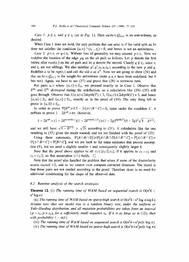
104 P.L. Erd6s et al. / Theoretical Computer Science 221 (1999) 77-118
Case 1: p q~ tl and q q~ t2 (as & Fig. 1). Then auIbvEQw(~) is an anti-witness, as desired.
When Case 1 does not hold, the only problem that can arise is if the valid split aulbv does not satisfies the condition {u,v} n ( q U t 2 ) = 0, and hence is not an antiwitness.
Case 2: p E tl or q c t2. Without loss of generality we may assume p E tt. Now we redefine the location of the edge pq on the ab path as follows. Let p denote the first
vertex after root(tl ) on the ab path and let q denote the second. Clearly q ~ t2, since tl
and t2 are not siblings. We also redefine p~, q~, t3, u, t4, v according to the new p and q. Redefine a to be rep(tl ) and call the old a as a*. Now we are going to show (26) and
that auibv E Qw(~) is the sought-for antiwitness (note a, u, v have been redefined, but b has not). Again, we have to see (27) and prove that (28) is termwise zero.
For pairs u,v where {u,v} C $2~, we proceed exactly as in Case 1. Observe that
E bu and E 6~' decreased during the redefinition, so a calculation like ( 2 9 ) - ( 3 5 ) still goes through. Observe that L( a, u) <~ 2depth(T) + 2, L( a, v) <~ 2depth(T) + 3, and hence
{a,u}ES2~ and {a,v}ES2~, exactly as in the proof of (19). The only thing left to prove is {a,b} E S2r.
In order to prove P[h ab > / 0 . 5 - 2~IA n B n C] = 0 , since under the condition C, it suffices to prove 1 - 2 E a b > 6~. However,
1 - 2E ab = (1 - 2E a'r°°t('' ))(1 - 2E r°°t(t' ),b)/> ( 1 - 2g)depth(T)(1 -- 29) 2 V/1 -- E a* b,
and we still have v / 1 - E a*b > v ~ according to (31). A calculation like the one resulting in (35) gives the result wanted, and we are finished with the proof of (23).
Using these statements, P [ A N B N D ] > , P [ A N B N D I A N B N C ] × f f ~ [ A N B N C ] =
~[A n B N C] = P[B n C], and we are back to the same estimates that proved assump- tion (9), but we need a slightly smaller r and consequently slightly larger k.
Note that the proof above applies to all c3 E [c2/2,c2], if it applies to c3 =c2 and c3 = c2/2, so that assumption (11) holds. []
Note that the proof also handled the problem that arises if some of the dissimilarity scores exceed 1/2, and so we cannot even compute corrected distances. The moral is that those pairs are not needed according to the proof. Therefore there is no need for additional conditioning for the shape of the observed data.
6.2. Runt ime analysis o f the search strategies
Theorem 12. (i) The running time o f W A M based on sequential search is O(n2k -I- n 6 log n)
(ii) The running time o f W A M based on sparse-high search is O(n2k +n 4 log n log k). Assume now that our model tree is a random binary tree, under the uniform or
Yule-Harding distribution, and all mutation probabilities are taken f r o m an interval
( p - e,n,p + en) , for a sufficiently small sequence ~. I f k is as large as in (12), then with probability 1 - 0(1 )
(iii) The running time o f W A M based on sequential search is O(n2k +n3poly log n). (iv) The running time o f W A M based on sparse-high search is O(n2k +n2poly log n).

P.L. Erdrs et al. / Theoretical Computer Science 221 (1999) 77-118 105
Proof. Computing the matrices h and d takes O(n2k) time. (All distance methods begin by computing these distance matrices, but this "overhead cost" is usually always mentioned in the running time analysis of a given method.) Let w0 be defined to be the smallest w C h ij such that Qw is T-forcing. Let i(w) be the order of w within the sorted h ij values. Then, since each call of the WATC algorithm uses O(n2+ [Q[ log IQ])
time, the running time of the sequential search is O(i(wo)(n 2 + IQwol log Iawol)), after
the preprocessing. For (i), the sequential search application of the WATC algorithm is O(n61ogn),
since we need never do more than examine all sets Qw, and the largest such set has cardinality O(n4).
Claim (ii) follows form the observations that the sparse-high search calls the WATC algorithm at most O(log k) times, and each call costs at most O(n 4 log n) time.
We now prove (iii). The depth of a random tree (under either the uniform or Yule- Harding distributions) is with high probability O(log log n) by Theorem 10, and so there are at most O(polylogn) leaves which are no more than about O(loglogn) distance (measured topologically) from any fixed leaf. This is the only fact that we exploit from the assumption of randomness of the tree. For two leaves i,j, recall that L(i , j) denotes the topological distance between i and j. We are going to show that if r is the value at which the search reconstructs the tree in the proof of Theorem 11, then with probability 1 - o ( 1 ) we have L( i , j )= O(log log n), whenever i , j c q c Qr. This yields IQwl~)l =n .polylog(n). In the proof of Theorem 11, according to formula (18), event C holds with probability 1 - o ( 1 ) . In that proof Qw(~) is denoted by Z~/4. Now
(1 - 2q) L(i'j)= 1 -- 2E ij >~ z/2, (36)
where the equality follows from Lemma 1, and the inequality follows from the condi- tioning on the event C. Plugging in (35) for z immediately yields L ( i , j )= O(log log n). Since the sequential search makes O(npolylog(n)) calls to the WATC algorithm, (iii)
follows. To obtain (iv), observe that Formulae (35), (17), and depth(T)= O(log log n) imply
that the number of iterations in the sparse-high search is
- log 2 z = O ( - log(1 - 29). depth(T)) = O(log log n). []
6.3. The performance of other distance methods under the Neyman 2-state model
In this section we describe the convergence rate for the WAM and DCM method, and compare it briefly to the rates for two other distance-based methods, the Agarwala et al. 3-approximation algorithm [1] for the L~-nearest tree, and neighbor joining [43]. We make the natural assumption that all methods use the same corrected empirical distances from Neyman 2-state model trees. The comparison we provide in this section will establish that our method requires exponentially shorter sequences in order to ensure accuracy of the topology estimation than the algorithm of Agarwala et al., for almost all trees under uniform or Yule-Harding probability distributions. The trees for which the two methods need comparable sequence lengths are those in which the

106 P.L. Erdrs et al. / Theoretical Computer Science 221 (1999) 77-118
diameter and the depth are as close as possible - such as complete binary trees. Even in these cases, WAM and DCM will nevertheless need shorter sequences than Agarwala
et al. to obtain the topology with high probability, as we showed it in Section 3. (Again, note that this analysis is inherently pessimistic, and it is possible that the methods may obtain accurate reconstructions from shorter sequences than suffice by this analysis.)
The neighbor joining method is perhaps the most popular distance-based method
used in phylogenetic reconstruction, and in many simulation studies (see [34, 35, 44] for an entry into this literature) it seems to outperform other popular distance based
methods. The Agarwala et al. algorithm [1] is a distance-based method which provides
a 3-approximation to the L ~ nearest tree problem, so that it is one of the few methods which provide a provable performance guarantee with respect to any relevant optimiza-
tion criterion. Thus, these two methods are two of the most promising distance-based methods against which to compare our method. All these methods use polynomial time.
In [22], Farach and Kannan analyzed the performance of the Agarwala et al. algo- rithm with respect to tree reconstruction in the Neyman 2-state model, and proved that
the Agarwala et al. algorithm converged quickly for the variational distance. Personal communication from S. Kannan gave a counterpart to (12): if T is a Neyman 2-state model tree with mutation rates in the range [ f , g], and if sequences of length k' are generated on this tree, where
c ~ • log n k' > f2(1 _ 2g)2diam(T ) (37)
for an appropriate constant c/, and where diam(T) denotes the "diameter" of T, then with probability 1 - o(1 ) the result of applying Agarwala et al. to corrected distances will return the topology of the model tree. In [5], Atteson proved the same result for Neighbor Joining though with a different constant. (The constant for neighbor joining is smaller than the constant for the Agarwala et al. algorithm, suggesting that neigh-
bor joining can be guaranteed to be accurate from shorter sequences than Agarwala
et al., on any tree in the Neyman 2-state model. However, remember that this anal- ysis is pessimistic, and it may be that correct reconstruction is possible from shorter sequences than this analysis suggests.)
Comparing this formula to (12), we note that the comparison of depth and diam- eter is the issue, since (1 - lxfi--L-~-2f)2 = E ) ( f 2) for small f . It is easy to see that
diam(T)>>.2depth(T) for binary trees T, but the diameter of a tree can in fact be quite
large (up to n - 1), while the depth is never more than log n. Thus, for every fixed range of mutation probabilities, the sequence length that suffices to guarantee accuracy for the Neighbor Joining or Agarwala et al. algorithms can be quite large (i.e. it can grow exponentially in the number of leaves), while the sequence length that suffices for the witness-antiwitness method will never grow more than polynomially.
In order to understand the bound on the sequence length needed by these methods, we now turn to an analysis of the diameter of random trees. The models for random trees are the uniform model, in which each tree has the same probability, and the

P.L. Erdrs et al. I Theoretical Computer Science 221 (1999) 7~118 107
Yule-Harding model, studied in [2, 8, 29]. This distribution is based upon a simple model of speciation, and results in "bushier" trees than the uniform model.
Theorem 13. (i) For a random semilabelled binary tree T with n leaves under the
uniform model, diam( T) > ev/-n with probability 1 - O(e.2). (ii) For a random semilabelled binary tree T with n leaves under the Yule-Harding
distribution, after suppressing the root, diam( T ) : O(log n ), with probability 1 -o (1) .
Proof. We begin by establishing (i). The result of Carter et al. [11] immediately implies that leaves a, b have distance m+l with probability exactly m!N(n-2 , m) / (2n -
5)!! under the uniform model. For small enough e, m ~< ev/-n, this probability is O(m/n). Summing up the probabilities from m = 1 to m = ex/-n, we see that diam(T)>ex/~ with probability at least 1 -O(e2) .
We now consider (ii). First we describe rooted Yule-Harding trees. These trees are defined by the following constructive procedure. Make a random permutation hi, n2 . . . . , n, of the n leaves, and join nl and n2 by edges to a root R of degree 2. Add each of the remaining leaves sequentially, by randomly (with the uniform probability) selecting an edge incident to a leaf in the tree already constructed, subdividing the edge, and make ni adjacent to the newly introduced node. For a rooted Yule-Harding tree T R, let h(T R) denote the maximum distance of any leaf from the root. Let T be the unrooted Yule-Harding tree obtained from T R by suppressing the root, and iden- tifying the two edges incident with the root. Let diam(T) denote the diameter of T. Then, we always have
h(TR)<~diam(T)<<.2h(T R) - 1.
Now Aldous [2] shows that h(TR)/log n converges in distribution to a (nonzero) constant c. Then, with probability tending to 1, diam(T)/log n will lie between c and 2c. []
In Table 1, we summarize sequence length that suffice for accurate reconstruction with high probability of WAM and DCM, and compare these to the sequence lengths that suffice for the Agarwala et al. algorithm, according to the analyses that we have given above (thus, our summary is based upon (12), (37), and Theorems 10 and 13). Sequence lengths are given in terms of growth as a function of n, and assume that mutation probabilities on edges lie within the specified ranges.
7. Extension to general stochastic models
In this section we consider the generalization of the WAM and DCM for inferring trees in the general stochastic model. Just as in the case of the Neyman 2-state model, we find that WAM and DCM obtains accurate estimations of the tree from sequences whose length is never more than polynomial in the number of leaves (for every fixed

108
Table 1
P.L. Erdrs et al./Theoretical Computer Science 221 (1999) 77-118
Range of mutation probabilities on edges
[f, 9] I 1 log log n ] f , g are constants Llog n' ~ ]
Binary trees DCM/WAM Polynomial Polylog Worst-case Agarwala et al. Superpolynomial Superpolynomial Random binary trees DCM/WAM Polylog Polylog (uniform model) Agarwala et al. Superpolynomial Superpolynomial Random binary trees DCM/WAM Polylog Polylog (Yule-Harding) Agarwala et al. Polynomial Polylog
range for the mutation probabilities), and in general only polylogarithmic in the number of leaves. This should be contrasted to the study of Ambainis et al. [4].
Suppose the sequence sites evolve i.i.d, according to the "general" Markov model - that is, there is some distribution of states rc at the root of the tree, and each edge e has an associated stochastic transition matrix M(e), and the (random) state at the root evolves down the tree under a natural Markov assumption, as in the general stochastic model of Definition (III).
Let J~j(~, r ) denote the probability that leaf i is in state ~ and leaf j is in state ft. By indexing the states, J~j(~, r ) forms a square matrix, F/j = [fij(a, fl)]. Then
c~ii = - log det(F/j) (38)
denotes the corrected model distance between i and j . (There will be a guarantee for det(Fij) > 0.)
The corrected empirical distance ~ij of two species is computed as in (38), but uses
the matrix ff'ij composed of the relative frequencies fq(ct, r ) of i being in state a and j being in state r , instead of the probability J~j(a, fl):
(~ij = -- log det(Fij). (39)
Then, dPij can be derived from a positive edge weighting of the model tree, provided that the identifiability condition described in Section 2 (Tree Reconstruction) holds. These mild conditions only require that det(M(e)) not take on the values 0, 1 , - 1, and that the components of ~z are nonzero (i.e. every state has a positive probability of occurrence at the root).
Note that det(M(e)) takes the values 1 or - 1 precisely if M(e) is a permutation matrix. Also, for the Neyman 2-state model det(M(e)) -- 1 - 2p(e), where p(e) is the mutation probability on edge e; thus, de t (M(e) )>0 and det(M(e)) tend to 0 as p approaches 0.5, and tend to 1 as p approaches 0. In general, (1/2)[1 -de t (M(e)] plays the role of p(e) in the general model. Thus, a natural extension of our restriction f<. p(e)<~9 and from the Neyman 2-state model corresponds to
0 < 1 - 2x I ~< det(M(e)) ~< 1 - 2x < 1, (40)

P.L. Erdds et al. I Theoretical Computer Science 221 (1999) 77-118 109
for suitable x,x ~, and we will henceforth impose this restriction for all edges of the tree. For technical reasons, we also impose the mildly restrictive condition that every vertex can be in each state p with at least a certain fixed positive probability:
7r(v)~ >e,. (41)
This condition (41) certainly holds under the Neyman 2-state model, the Kimura 3- state model [39], and much more general models (providing each state has positive probability of occurring at the root). Indeed this last weaker condition might be enough, but it would seem to complicate the analysis quite a lot.
Now, let Z(e) be the weight of edge e in the realization of ~b on the (unrooted version) of the true underlying tree T.
Lemma 4. Set 6 ( x ) = - 0 . 5 log(1 - 2 x ) . Then
2(e) 7> - 0.5 log(det(M(e))) ~> 3(x)
for every edge e of T.
(42)
Proof. The second inequality follows from the restriction we imposed above on det(M(e)). The first inequality in (42) follows from similar arguments to those ap- pearing in [47]; for the sake of completeness we give a proof.
Let T be the unrooted version of TP. Now the edges of T correspond bijectively to the edges of T p, except perhaps for one troublesome edge of T which arises whenever the root of T p has degree two - in that case, two edges el, e2 of TP adjacent to p are identified to form e. For convenience, we assume in this proof that p is not a leaf.
We now prove that 2(e)~> - 0 . 5 log det(M(e)) for all (non-troublesome) edges e of T, and if T has a troublesome edge e corresponding to edges el and e2 in TP, then ).(e) >~ - 0.5 log(det(M(el )) det(M(e2))).
For any edge e=(v,w) of TP where w is a leaf, let
while, for any edge e=(v,w) of TP for which neither of v, w are leaves, let
h(e)=-logdet(M(e))-O.51og[~rf fv) , 1 + 0.5 log [ ~ ~(w),] .
Thus, h describes a weighting of the edges of TP and thereby a weighting h* of the edges of T by setting h* equal to h on the non-troublesome edges, and the convention that if T has a troublesome edge e arising from the identification of a pair el, e2 of edges of T p then h*(e)=h(el)+ h(e2). Now, h realizes the 4~ij values on T p. Thus, h* also realizes the q~ij values, on T and since (as we show) the edge weighting is strictly positive, it follows, by classical results [10], that this is the unique such edge weighting of T. Thus 2 = h*.

110 P.L. Erdds et al. I Theoretical Computer Science 221 (1999) 77-118
Now for an edge e=(v,w) of TP where w is a leaf,
h(e) >1 - log det(M(e)) >~ - 0.5 log det(M(e))
as claimed. Alternatively, for an edge e = (v, w) of T for which neither of v, w are
leaves, we have
h(e)=-logdet(M(e))-0.5log I~rt(v)~ ] + 0.5log I ~ ( w ) ~ l .
In order to derive our desired inequality we establish a further result. Let us suppose M = [M~v] is any r × r matrix with non-negative entries and x is a row vector of length
r with non-negative entries. We claim that
1~ (xM),, ~> Idet(M)ll~ xu.
To obtain this, note that the left-hand side is just
~ (~v XvMvp) >J (~Ma(l'lM~r(2'2""Mff(r)r) ~xl z'
where the second summation is over all permutations a of (1,2 . . . . . r), and so this sum is at least [det(M)], since the permanent of a nonnegative matrix is never smaller than the absolute value of its determinant. Now, [z(w)l . . . . . z(w)r] = [Tr(V)l . . . . . rt(V)r]M(e), and so, applying the above inequality to the case M = M ( e ) and x = [z(V)l . . . . . rc(v)r],
we obtain
I] rc(w)~/> det(M(e))I- I re(v),.
Thus,
0.51ogdet(M(e))~O.51og[~(W)v]-0.5 log [ ~ 7z(v)~]
and so
h(e) = -0.5 log det(M(e))
] /> -0.5 log det(M(e)),
as claimed. The inequalities for h now extend to h * = 2 for all (non-troublesome) edges of T.
If T p has a troublesome edge e then 2 (e )= h*(e)= h(el )+ h(e2), and from the above we have h(ei)>- -0.51ogdet(M(ei)) for i = 1,2. []

P.L. Erd6s et al. I Theoretical Computer Science 221 (1999) 77-118 111
Theorem 14. Let x = x ( n ) and x ~ =xt(n) be such that f o r all edges in the tree T,
0 < 1 - 2x ~ ~< det(M(e)) ~< 1 - 2x < 1. Assume x ~ has an upper bound strictly less than
1/2. Mutat is mutandis, algorithms F P M , D C M and W A M , Theorems 9, 11, and 12 generalize to the general stochastic model under (40) and (41). W A M and D C M
returns the binary model tree T with probability 1 - o(1 ) i f
c • l o g n
k > x2 ( 1 - 2x t )4depth(T) (43)
with a certain constant c.
^
definition of the corrected empirical distance, q~ij, Proof. Recall the and 6(x) ( = - 0 . 5 log(1 - 2 x ) ) . We first establish the following
Claim: I f
[ff)ij -- ~)ijl > 6(x)/2 (44)
then
] det(Fij) - det( Pij)l >x det(U j)/4. (45)
Proo f o f Claim: By inequality (44),
1 /'det(FiJ ) ) ~1 [ log(det (XiJ)) - log(det(PU))l = o g ~ _ > - log(1 - 2x)
and so det(f "ij)/det(F ij ) is either greater than (1-2x)-1/4, or less than (1 - 2x) 1/4. Thus, [det(F ij) - det(FiJ)l > min{~-(x), ~+(x)} det(F ij) where ~+(x):= 1 - (1 - 2x)1/4; ~- = ( 1 - 2x) -1/4 - 1. Now, it can be checked that, for x strictly between 0 and 1/2, ~- (x ) , c~+(x)>x/4 which establishes the Claim.
To apply Lemma 3, we need to know how det(F i j) responds to the replacement at one site of a pattern by a different pattern. If ~iJ is the resulting F-matrix for this perturbed data set, then
FII ij = 1 ~ij ~- (1/k )D ij
where D ij has one entry of + 1, one entry of - l , and all other entries O. Consequently,
i det(~ij) _ det(/~ij)l ~< c l/k (46)
for some constant Cl. Next, for any real analytic function f defined on a vector x having a normalized
multinomial distribution with parameters k and p, we have (by Taylor expansion of f about p to the second derivative term, followed by application of the expectation operator):
1 M , s I~=[f(x)] - f(tOI < ~ .~ Icov(xi,xs)[,

112 P.L. Erd~s et al. / Theoretical Computer Science 221 (1999) 77-118
where COU(Xi,Xj) is the covariance of xi,x j (equal to /2i(1 - -#i) /k , when i= j , and -I~i#jk otherwise); and where M is the maximal value of any of the second derivatives of f over the unit simplex. Thus, since det(F ij) is a polynomial in the entries of F i j, we have:
I E[det( pij )] - det( Fij )l ~< c2/k (47)
for some constant c2. Combining (47) with the triangle inequality gives
Idet(F ij) - det(/6iJ) I ~< I det(P 'J) - E[det(FiJ)] I + c2/k
and so
P[Idet(Fij) - det( p'J)I > t] ~< P[Idet(pij) - E[det(F ~j)]l > (t - c=/k)] (48)
for any t > 0 . Hence by Lemma 3, applied with (46), we have
f "fxdet(FiJ)~ -4 c232k)k ~[I det(Fij) - det(ff'iJ)l >xdet(gij)/4] ~<2 exp ~ - a (49)
for a constant d. For the validity of the latter argument we need that
xdet(F ij) cz >0. (50) 4 k
Now, how can we set a lower bound for det(FiJ)? Note that det(F ij) is just the product of det(M(e)) over all edges on the path from i to j , times the product of ~(vij)~ over all states #, where rffv) is the vector of probabilities of states at vertex v, and v 6 is the most recent common ancestor of i and j in the tree. Due to our hypotheses (41), we have
det F ij > c3 (1 - 2x' )d(i'J) (51 )
with a positive constant c3. However, the conditions of the Theorem required k > cx- 1
(1 --2xt) -d(i'j), and therefore taking a sufficiently large c guarantees (50).
Putting the pieces (44), (45) and (49) together we see that
Combining (51) and (42), we have
2) (52)
4
where c4 is a positive constant, and d(i,j) is the number of edges in T separating leaves i and j . Hence, for any fixed quartet q of diameter diam(q),
~[FPM errs on q] <~Kexp(-D'x2(1 -2xt)2diam(q)k) (53)
for constants D',K. Thus we have an analogue of Theorem 9.

P.L. Erdrs et al. / Theoretical Computer Science 221 (1999) 77-118 113
Now we show how to generalize the proof of Theorem 11. To avoid needless rep- etitions, we give details for the proof of assumption (9) only, and leave the proofs of assumptions (10) and (11) to the Reader. Note that the proof of correctness of DCM hinges exactly on assumption (9). Having a distance function in the general model, the width and algorithmic operations based on width generalize in a straightforward
way. For k evolving sites (i.e. sequences of length k), and r > 0 , let us define the follow-
ing two sets, ST = {{i,j}: det(F ij) > 2z} and Z~ = {q E ([41): for all i , j C q, { i , j } c S2z} (note the similarity between the definition for the set Z~, and that for the set Qw of quartet splits of quartets of width at most w). We also define the following two events, A = {Qshort(T)C_ Z~} and B = FPM correctly reconstructs the tree for all q E Z~. Thus, P[~/N ~ ¢ ~] ~> P[A ?? B]. Let C be the event: "$2~ contains all pairs { i , j } with det(F ij) > 6r, and no pair { i , j } with det(F ij) ~ 2r". Define 2 = el( 1 - 2x')2depth(r 1+3.
We claim that
P[C] ~> 1 - ( n 2 - n)e -cdk (54)
for a constant c > 0 and
IP[AIC ] = 1 if z~<2/6. (55)
Suppose det(FiJ)<~2z. To establish (54), using arguments similar to those between
(45) and (49) one easily sees that Lemma 3 applies and
P[{i,j} C $2~] = P[det(F ij) >4z]
~< P[det(F ij) - det(F ij) >~ 2z] ~< e -¢~2k
for a constant c > 0. Since there are at most (2) such pairs { i , j } such that det(FiJ)<.2z, the probability
that at least one such pair lies in $2~ is at most (2) e-C~2k" By a similar argument, the probability that $2~ fails to contain a pair {i,j} with det(FiJ)>6z is also at most
n --cz2k (2)e . These two bounds establish (54). We now establish (55). For q C Qshort(T) and i , j E q, if a path ele2.. , et joins leaves
i and j , then t <~ 2dep th(T)+ 3 by the definition of Q s h o r t ( T ) . Using these facts, and the bound det(M(e)) ~> 1 - 2x ~, we obtain det( F ij ) >~ e r ( 1 - 2x' )t. Consequently, det( F ij ) > 6z
(by assumption that z ~<2/6 ) and so {i,j} E $2~ once we condition on the occurrence of event C. This holds for all i , j E q, so by definition of Z~ we have q E Z~. This
establishes (55). Then for any quartet q E Qshort(T), if e is the central edge of the contracted subtree
induced by q in T, then det(M(e))~< 1 - 2 x . Furthermore, conditional on C, for any pendant edge e, de t (M(e ) )> min{det(FiJ): i, j C q } > 2 z . Thus, by (53), which is the analogue of Theorem 9, and the Bonferroni inequality, we can follow the corresponding

114 P.L. Erd6s et al. / Theoretical Computer Science 221 (1999) 77-118
proof from Theorem 11, to obtain (using (54) and (55))
n P[A fq B] ~>1 - K ( 4 ) exp(-D'x2(1 - 2Xt)2depth(T)+3k) -- (n2 - n)e-a~)k
for constants K,D'> 0 Formula (43) now follows by an easy calculation. Note that the proof also handled the problem that arises if some logarithms are to
be taken of negative numbers and so we cannot even compute corrected distances. The morale is that those pairs are not needed according to the proof. Therefore there is no need for additional conditioning for the shape of the observed data.
8. Considerations for biological data analysis
The focus of this paper has been to establish analytically that every evolutionary tree is accurately reconstructable from quartets of closely related taxa, and, furthermore, this requires just very short sequences, given certain assumptions about the model tree. This is a significant theoretical result, especially since the bounds that we obtain indicate that the sequence lengths that suffices for accuracy with high probability using our new methods are very much shorter than those that suffice for accuracy using other very promising distance-based methods. However, are these observations significant for biological datasets? And if they are, are these methods likely to be practically useful (or merely indications of what might be achieved in future)?
The answer to the first question, concerning the significant for biological datasets, de- pends upon whether there are biologically realistic evolutionary trees that have smaller "weighted depth" than "weighted diameter", a concept that we now define.
Let T be an edge-weighted tree with positive weights on the internal edges and non-negative weights on the edges incident with leaves. Let e be an internal edge of the tree. The weighted depth around edge e is the minimum value of q so that there exists a set of four leaves, i,j, k, I, with one leaf in each of the four subtrees induced
T T T T T T by the removal of e and its endpoints, where q = max{dij, dik,dit, d~k,d~t, dkl }. The weighted depth of the tree T is then the maximum weighted depth of any edge in T. The weighted diameter of a tree T is simply the maximum dxry, taken over all pairs of leaves x,y. We will denote the weighted depth of a tree T by wdepth(T) and its weighted diameter by w diam(T).
The analysis given in the previous sections of the sequence length that suffices for accuracy for various methods can be restated as follows:
Corollary 1. D C M and WAM will be accurate with probability 1 - 6 if the sequence length exceeds
c log n e O(wdepth(T)),
where c is a constant that depends upon only f = mine p(e) and 6. The other distance based methods (Agarwala et al. 's single-pivot algorithm and its variant, the double-

P.L. Erd6s et al. / Theoretical Computer Science 221 (1999) 77-118 115
pivot algorithm, the naive method, and neighbor-joining) are accurate with the same
probability i f the sequence length exceeds
c t log ne O(wdiam(T)),
where c' is a constant that also depends only upon f = mine{p(e)} and 6.
These are only upper bounds (i.e. these may be loose, and exact accuracy may be possible from shorter sequences), but these are also currently the best upper bounds that are known for these methods, to our knowledge.
Thus, to compare the sequence lengths that suffice for exact topological accuracy, we need to compare the weighted depth to the weighted diameter. A reasonable comparison between these two quantities for biologically realistic trees is difficult, as there are very few well established evolutionary trees, especially of large divergent datasets. On the other hand, for some data sets, evolution may proceed in a more-or-less clock-like fashion (i.e. the number of mutations that occurs along an evolutionary lineage is roughly proportional to time). For such data sets, it can be seen that the weighted depth and the weighted diameter are exactly the same. Under these circumstances, there is no benefit to using DCM or WAM instead of one of the better other distance methods, such as neighbor joining, although this analysis also does not suggest that neighbor joining will outperform DCM or WAM (to be precise, the conditions that guarantee accuracy for neighbor-joining will also guarantee accuracy for DCM and WAM, and vice versa). Thus, for clock-like evolutionary conditions, these techniques do not provide any advantage from a theoretical standpoint.
On the other hand, there are important biological data sets for which evolution pro- ceeds in a very non-clock like fashion, according to various analyses by biologists and statisticians (see, for example, [55, 56]). For these data sets, there could be significant advantage obtained by using techniques such as DCM and WAM, which examine only closely related taxa in order to reconstruct the tree. The degree to which DCM and WAM could provide an advantage would theoretically depend upon the magnitude of the difference between the weighted depth and weighted diameter. This magnitude is likely to be largest for sets of highly divergent taxa, rather than for closely related taxa.
As a practical tool, DCM and WAM are not entirely satisfactory, in part because DCM and WAM only return trees when the conditions hold for exact accuracy. Al- though some biologists would rather get no tree than get an incorrect tree [41], not all biologists share this view, and so partially correct trees are often desirable. Thus, the answer to the second question is basically negative.
However, DCM and WAM were not designed to be practical tools, but rather to indicate theoretical possibilities, and to suggest how better methods might be invented which could have the theoretical guarantees that DCM and WAM provide, while having better performance in practice. Furthermore, such methods have recently been devel- oped. The disk-covering method of Huson et al. [36] the harmonic greedy triples
method of Csuros and Kao [16], and the method of Cryan et al. [15] have each used

116 P.L. Erd.rs et aL / Theoretical Computer Science 221 (1999) 77-118
the observations in this paper and obtained methods with convergence rates that are never worse than polynomial by using only small distances to (re)construct the tree.
Acknowledgements
We thank Scott Nettles for fruitful discussions of efficient implementations, and David Bryant and l~va Czabarka for proof reading the manuscript. We also thank A. Ambainis and another (anonymous) referee, for their careful reading of the manuscript and helpful suggestions for improving the exposition.
P&er L. Erdfs was supported in part by the Hungarian National Science Fund con- tract T 016 358. L~iszl6 A. Szrkely was supported by the National Science Foundation grant DMS 970121 l, the Hungarian National Science Fund contracts T 016 358 and T 019 367, and European Communities (Cooperation in Science and Technology with Central and Eastern European Countries) contract ERBCIPACT 930 113. Michael A. Steel was supported by the New Zealand Marsden Fund and the New Zealand Ministry of Research, Science and Technology. Tandy J. Warnow was supported by an NSF Young Investigator Award CCR-9457800, a David and Lucille Packard Foundation fel- lowship, and generous research support from the Penn Research Foundation and Paul Angello.
This research started in 1995 when the authors enjoyed the hospitality of DIMACS during the Special Year for Mathematical Support to Molecular Biology, and was completed in 1997 while enjoying the hospitality of Andreas Dress, at Universitiit Bielefeld, in Germany.
References
[1] R. Agarwala, V. Bafna, M. Farach, B. Narayanan, M. Paterson, M. Thorup, On the approximability of numerical taxonomy: fitting distances by tree metrics, in: Proc. 7th Annual ACM-SIAM Symp. on Discrete Algorithms, 1996, pp. 365 372.
[2] D.J. Aldous, Probability distributions on cladograms, in: D.J. Aldous, R. Permantle (Eds.), Discrete Random Structures, IMA Volume in Mathematics and its Applications, vol. 76, Springer, Berlin, 1995, pp. 1-18.
[3] N. Alon, J.H. Spencer, The Probabilistic Method, Wiley, New York, 1992. [4] A. Ambainis, R. Desper, M. Farach, S. Kannan, Nearly tight bounds on the leamability of evolution,
in: 38th Annual Symp. on Foundations of Computer Science, Miami Beach, FL, 20-22 October 1997. IEEE Science, New York, pp. 524-533.
[5] K. Atteson, The performance of neighbor-joining algorithms of phylogeny reconstruction, in: Computing and Combinatorics, 3rd Annual Intemat. Conf., COCOON'97, Shanghai, China, August 1997, COCOON'97, Lecture Notes in Computer Science, vol. 1276, Springer, Berlin, pp. 101-110.
[6] H.-J. Bandelt, A. Dress, Reconstructing the shape of a tree from observed dissimilarity data, Adv. Appl. Math. 7 (1986) 309-343.
[7] V. Berry, O. Gascuel, Inferring evolutionary trees with strong combinatorial evidence, in: Computing and Combinatorics, 3rd Annual Intemat. Conf., COCOON'97, Shanghai, China, August 1997, COCOON'97, Lecture Notes in Computer Science, vol. 1276, Springer, Berlin, pp. 111-123.
[8] J.K.M. Brown, Probabilities of evolutionary trees, Syst. Biol. 43 (1994) 78-91. [9] D.J. Bryant, M.A. Steel, Extension operations on sets of leaf-labelled trees, Adv. Appl. Math. 16 (1995)
425-453.

P. L. Er d6s et al. I Theoretical Computer Science 221 (1999) 77-118 117
[10] P. Buneman, The recovery of trees from measures of dissimilarity, in: F.R. Hodson, D.G. Kendall, P. Tautu (Eds.), Mathematics in the Archaeological and Historical Sciences, Edinburgh University Press, Edinburgh, 1971, pp. 387-395.
[11] M. Carter, M. Hendy, D. Penny, L.A. Szrkely, N.C. Wormald, On the distribution of lengths of evolutionary trees, SIAM J. Discrete Math. 3 (1990) 38-47.
[12] J.A. Cavender, Taxonomy with confidence, Math. Biosci. 40 (1978) 271-280. [13] J.T. Chang, J.A. Hartigan, Reconstruction of evolutionary trees from pairwise distributions on current
species, in: Computing Science and Statistics: Proc. 23rd Symp. on the Interface, 1991, pp. 254-257. [14] H. Colonius, H.H. Schultze, Tree structure for proximity data, Br. J. Math. Statist. Psychol. 34 (1981)
167-180. [15] M. Cryan, L.A. Goldberg, P.W. Goldberg, Evolutionary trees can be learned in polynomial time in
the two-state general Markov-model, in: Proc. 39th Annual IEEE Symp. on Foundations of Computer Science, 1998, pp. 436-445.
[16] M. Csuros, M.-Y. Kao, Fast reconstruction of evolutionary trees through Harmonic Greedy Triplets, in: Proc. ACM-SIAM Symp. on Discrete Algorithms, 1999, pp. 261-268.
[17] W.H.E. Day, Computational complexity of inferring phylogenies from dissimilarities matrices, Inform. Process. Lett. 30 (1989) 215-220.
[18] P.L. Erdrs, M.A. Steel, L.A. Szrkely, T. Warnow, Local quartet splits of a binary tree infer all quartet splits via one dyadic inference rule, Comput. Artif. Intell. 16 (2) (1997) 217-227.
[19] P.L. Erdrs, M.A. Steel, L.A. Szrkely, T. Warnow, Inferring big trees from short quartets, in: ICALP'97, 24th Internat. Colloquium on Automata, Languages, and Programming, Silver Jubilee of EATCS, Bologna, Italy, July 7-11, 1997, Lecture Notes in Computer Science, vol. 1256, Springer, Berlin, 1997, pp. 1-11.
[20] P.L. Erdrs, M.A. Steel, L.A. Szrkely, T. Warnow, A few logs suffice to build (almost) all trees (1), Random Struct. Algorithms 14 (1999) 153-184.
[21] M. Farach, J. Cohen, Numerical taxonomy on data: experimental results, in: Proc. ACM-SIAM Symp. on Discrete Algorithms, 1997.
[22] M. Farach, S. Kannan, Efficient algorithms for inverting evolution, in: Proc. ACM Symp. on the Foundations of Computer Science, 1996, pp. 230-236.
[23] M. Farach, S. Kannan, T. Warnow, A robust model for inferring optimal evolutionary trees, Algorithmica 13 (1995) 155-179.
[24] J.S. Farris, A probability model for inferring evolutionary trees, Syst. Zool. 22 (1973) 250-256. [25] J. Felsenstein, Cases in which parsimony or compatibility methods will be positively misleading, Syst.
Zool. 27 (1978) 401-410. [26] J. Felsenstein, Numerical methods for inferring evolutionary trees, Quart. Rev. Biol. 57 (1982) 379-404. [27] D. Feng, R. Doolittle, Progressive sequence alignment as a prerequisite to correct phylogenetic trees,
J. Mol. Evol. 25 (1987) 351-360. [28] Green Plant Phylogeny Research Coordination Group, Summary Report of Workshop #1: Current Status
of the Phylogeny of the Charophyte Green Algae and the Embryophytes (University and Jepson Herbaria, University of California, Berkeley, June 24-28, 1995), 1996.
[29] E.F. Harding, The probabilities of rooted tree shapes generated by random bifurcation, Adv. Appl. Probab. 3 (1971) 44-77.
[30] J. Hein, A new method that simultaneously aligns and reconstructs ancestral sequences for any number of homologous sequences, when the phylogeny is given, Mol. Biol. Evol. 6 (1989) 649-668.
[31] D. Hillis, Approaches for assessing phylogenetic accuracy, Syst. Biol. 44 (1995) 3-16. [32] D. Hillis, Inferring complex phylogenies, Nature 383 (1996) 130-131. [33] P. Hogeweg, B. Hesper, The alignment of sets of sequences and the construction of phylogenetic trees,
an integrated method, J. Mol. Evol. 20 (1984) 175-186. [34] J. Huelsenbeck, Performance of phylogenetic methods in simulation, Syst. Biol. 44 (1995) 17-48. [35] J.P. Huelsenbeck, D. Hillis, Success of phylogenetic methods in the four-taxon case, Syst. Biol.
42 (1993) 247-264. [36] D. Huson, S. Nettles, T. Wamow, Inferring very large evolutionary trees from very short sequences,
Proc., RECOMB, 1999. [37] T. Jiang, E. Lawler, L. Wang, Aligning sequences via an evolutionary tree: complexity and
approximation ACM STOC'94. [38] S. Kannan, personal communication.

118 P.L. Erdrs et al. / Theoretical Computer Science 221 (1999) 77-118
[39] M. Kimura, Estimation of evolutionary distances between homologous nucleotide sequences, Proc. Natl. Acad. Sci. USA 78 (1981) 454-458.
[40] J. Neyman, Molecular studies of evolution: a source of novel statistical problems, in: S.S. Gupta, J. Yackel (Eds.), Statistical Decision Theory and Related Topics, Academic Press, New York, 1971, pp. 1 27.
[41] K. Rice, personal communication. [42] K. Rice, T. Warnow, Parsimony is hard to beat, in: T. Jiang, D.T. Lee (Eds.), COCOON'97, Computing
and Combinatorics, 3rd Annual Internat. Conf., Shanghai, August 20-22, 1997, Lecture Notes in Computer Science, voh 1276, Springer, Berlin, pp. 124-133.
[43] N. Saitou, M. Nei, The neighbor-joining method: a new method for reconstructing phylogenetic trees, Mol. Biol. Evol. 4 (1987) 406-425.
[44] N. Saitou, T. Imanishi, Relative efficiencies of the Fitch-Margoliash, maximum parsimony, maximum likelihood, minimum evolution, and neighbor-joining methods of phylogenetic tree construction in obtaining the correct tree, Mol. Biol. Evoh 6 (1987) 514-525.
[45] Y.A. Smolensky, A method for linear recording of graphs, USSR Comput. Math. Phys. 2 (1969) 396 -397.
[46] M.A. Steel, The complexity of reconstructing trees from qualitative characters and subtrees, J. Classification 9 (1992) 91-116.
[47] M.A. Steel, Recovering a tree from the leaf colourations it generates under a Markov model, Appl. Math. Lett. 7 (1994) 19-24.
[48] M. Steel, M.D. Hendy, D. Penny, Reconstructing phylogenies from nucleotide pattern probabilities: a survey and some new results, Discrete Appl. Math. 89 (1999) 367-396.
[49] M.A. Steel, L.A. Szrkely, M.D. Hendy, Reconstructing trees when sequence sites evolve at variable rates, J. Comput. Biol. 1 (1994) 153-163.
[50] K. Strimmer, A. von Haeseler, Quartet Puzzling: a quartet Maximum Likelihood method for reconstructing tree topologies, Moh Biol. Evol. 13 (1996) 964-969.
[51] K. Strimmer, N. Goldman, A. von Haeseler, Bayesian probabilities and Quartet Puzzling, Mol. Biol. Evoh 14 (1997) 210 211.
[52] D.L. Swofford, G.J. OIsen, P.J. Waddell, D.M. Hillis, Phylogenetic inference, Ch. 11, in: D.M. Hillis, C. Moritz, B.K. Mable (Eds.), Molecular Systematics, 2nd ed., Sinauer Associates, Inc., Sunderland, 1996, pp. 407-514.
[53] D. Harel, R.E. Tarjan, Fast algorithms for finding nearest common ancestors, SIAM J. Comput. 13 (1984) 338-355.
[54] N. Takezaki, M. Nei, Inconsistency of the maximum parsimony method when the rate of nucleotide substitution is constant, J. Mol. Evol. 39 (1994) 210-218.
[55] L. Vawter, W. Brown, Nuclear and mitochondrial DNA comparisons reveal extreme rate variation in the molecular clock, Science 234 (1986) 194-196.
[56] L. Vawter, W. Brown, Rates and patterns of base change in the small subunit ribosomal RNA gene, Genetics 134 (1993) 597-608.
[57] L. Wang, D. Gusfield, improved approximation algorithms for tree alignment, J. Algorithms 25 (1997) 255-273.
[58] L. Wang, T. Jiang, On the complexity of multiple sequence alignment, J. Comput. Biol. 1 (1994) 337-348.
[59] L. Wang, T. Jiang, E. Lawler, Approximation algorithms for tree alignment with a given phylogeny, Algorithmica 16 (1996) 302-315.
[60] L. Wang, T. Jiang, D. Gusfield, A more efficient approximation scheme for tree alignment, in: Proc. 1st Annual lntemat. Conf. on Computational Molecular Biology, January 1997, Santa Fe, NM, USA.
[61] T. Warnow, Combinatorial algorithms for constructing phylogenetic trees, Ph.D. Thesis, University of California-Berkeley, 1991.
[62] M.S. Waterman, T.F. Smith, M. Singh, W.A. Beyer, Additive evolutionary trees, J. Theoret. Biol. 64 (1977) 199-213.
[63] A.C. Wilson, R.L. Cann, The recent African genesis of humans, Scientific Amer. 266 (1992) 68-73. [64] K.A. Zaretsky, Reconstruction of a tree from the distances between its pendant vertices, Uspekhi Math.
Nauk (Russian Mathematical Surveys) 20 (1965) 90-92 (in Russian).