A Feedback-Based Implementation Scheme for Batch

Process Optimization

E. Visser, B. Srinivasan, S. Palanki*, D. Bonvin ‡‡

Institut d’automatique, Ecole Polytechnique Federale de Lausanne,CH-1015 Lausanne, Switzerland.

*Florida State University, Tallahassee, Florida, USA.

The terminal-cost optimization of a control - affine nonlinear system leadsto a discontinuous solution that can be characterized in a piecewise man-ner. To implement such an optimal trajectory despite disturbances andparametric uncertainty, a cascade optimization scheme is proposed in thispaper, where optimal reference signals are tracked. Optimality is achievedby the appropriate definition of reference signals (input bounds, state con-straints, or switching functions) to track in various sub-intervals. Further-more, conservatism is introduced into the optimization problem to ensuresatisfaction of path constraints in the presence of uncertainty. Finally, theproposed cascade optimization scheme is illustrated on a simulation of afed-batch penicillin fermentation plant.

Key words: On-line optimization, Uncertainty, Feedback control, Optimal control,Batch process optimization

1 Introduction

A wide variety of specialty chemicals are made in batch reactors. To cope withcompetition, it is important to operate them in an optimal manner. The opti-mal operating policy for a given batch process is usually calculated under theassumption of a perfect model. However, realistic applications are subject touncertainty in initial conditions, model mismatch, and process disturbances,all of which affect the optimal solution. This provides the motivation for on-line calculation and implementation of the optimal operating policy. Also,recent developments in sensor technology has opened up new directions inprocess control and optimization. Thus, the availability of frequent measure-ments suggests a paradigm shift from open-loop model-based optimization toclosed-loop measurement-based optimization.

The two approaches to measurement-based optimization that have been pro-posed in the literature are discussed briefly below.

‡‡ Author to whom all correspondence should be addressed

Repeated optimization: Using this approach, the optimal inputs are updatedby solving a finite horizon optimization problem at each time step. The pa-rameters of the model required for the optimization are also estimated on-line.The solution to the optimization problem is either computed numerically [5] oranalytically [8]. Some of the drawbacks of this approach include: (i) high com-putational burden, especially in the presence of state and input constraints;(ii) necessity of full-state information; (iii) possible infeasibility of the solutionobtained [12]; (iv) conflict between parameter estimation which requires per-sistency of excitation and the optimization [11]; and (v) possible chattering ofthe feedback optimal solution [9].Cascade optimization: The optimal set-point trajectory that corresponds toperformance is computed. A ‘low level’ tracking controller ensures that thesystem does not stray very far away from the optimal trajectory [13,7]. Inaddition, a ‘high level’ optimizer is invoked periodically to ensure optimal-ity despite disturbances. This scheme, in general, requires neither full stateinformation nor on-line parameter estimation.

The cascade optimization approach combines the positive features of optimaloperation and feedback control. The basis of the cascade optimization schemeis tracking. Since there are typically more states than inputs, one cannot guar-antee that all the state trajectories will be accurately tracked in the presenceof disturbances. In general, a single combination of states that can be trackedduring the entire time interval does not exist. Instead, a piecewise definition ofthe outputs to track, i.e., different combinations of states/inputs for differenttime intervals, will be proposed.

Furthermore, conservatism has to be introduced in the optimization problemto guarantee feasibility in the presence of uncertainty. The use of margins fromconstraints, also called back-offs, and their computation as a function of theuncertainty will be developed within the framework of cascade optimization.

The paper is organized as follows. Section 2 formulates the problem. Section 3explains the cascade optimization framework in detail. The selection of outputsto track is treated in Section 4, and Section 5 discusses the conservatismrequired in the presence of uncertainty. Section 6 illustrates the approach viaa simulated example, and Section 7 concludes the paper.

2

2 Problem Formulation

The end-point optimization of a nonlinear, control - affine batch process canbe mathematically formulated as:

minu(t)

J = φ(x(tf )) (1)

s.t. x = f(x) +m∑i=1

gi(x) ui, x(0) = x0 (2)

S(x, u) ≤ 0 (3)

where u is the m-vector of manipulated inputs, x is the n-vector of states,f(x) and gi(x) are n-dimensional analytic vector fields. Also, the vector fieldsgi are assumed to be of full rank for all x. tf is the final time, φ is a smoothscalar function and S(x, u) is a σ-dimensional vector of path constraints. Notethat problem formulation (1) - (3) does not include terminal constraints.

Application of Pontryagin’s Minimum Principle (PMP) [3] to this end-pointoptimization problem involving a control-affine system, results in the followingHamiltonian:

H(x, u, λ) =λT(f(x) +

m∑i=1

gi(x)

)+ µTS(x, u) (4)

λT =−∂H∂x

= −λT(∂f

∂x+

m∑i=1

∂gi∂x

ui

)− µT ∂S

∂x(5)

λT (tf ) =∂φ

∂x

∣∣∣∣∣tf

(6)

where λ(t) 6= 0 is the vector of costates and µ(t) ≥ 0 are the Lagrangemultipliers for the state constraints and input bounds (µj > 0 only whenSj(x, u) = 0, j ∈ {1, · · · , σ}).The first-order necessary conditions for optimality are:

Hui = λTgi(x) + µT∂S

∂ui= 0, i = 1, · · · ,m (7)

Hui is independent of the inputs, if S(x, u) is affine in the manipulated inputvector, u. Thus, the necessary conditions, by themselves, cannot determine theinputs. For such problems, the optimal solution has the following properties:

– The inputs are in general discontinuous, yet inputs are analytic betweendiscontinuities.

– The solution between two discontinuities will be referred to as an arc. Threetypes of arcs are possible:

(i) inputs determined by active input bounds;(ii) inputs determined by active state constraints;

3

(iii) singular arc, when inputs are not determined by any of the active con-straints.

– Analytic expressions for these arcs can be obtained, though the sequenceand the switching times have to be computed numerically in most cases.

A piecewise analytic characterization of the optimal inputs helps to both im-prove the computational efficiency and to choose the implementation strategy.

Whether or not an arc is singular depends on the function ψi = λTgi(x), whichis referred to in the literature as the switching function. This function vanishesover the singular time interval. Outside the singular interval, the manipulatedinput ui(t) is on a state constraint or an input bound.

Methods for calculating the singular arcs are available in the optimal con-trol literature [8]. Since the switching function is zero over a time interval, itsderivatives with respect to time are also zero. Thus, a sequence of time differ-entiations is performed until the inputs ui(t) appear explicitly. The resultingexpression is then solved for ui(t) in terms of x and λ.

3 Cascade Optimization Framework

A cascade optimization structure is proposed to incorporate feedback into theoptimization framework (Figure 1). The ‘high level’ optimizer solves the op-timization problem and selects the appropriate outputs to track for specifictime intervals. Thus, it provides: (i) the feedforward inputs, u∗; (ii) the refer-ence signals, y∗; and (iii) the switching strategy between various subsequentoutputs. The optimizer constitutes the outer loop and is indicated by the thinlines in Figure 1. The reference signal of the corresponding output is thentracked with the help of the ‘low level’ feedback controller (inner loop - thicklines in Figure 1).

++

-

d

u

xu

y

y

Optimizer

ProcessFeedback

OutputConstruction

**

Fig. 1. Cascade Optimization

Due to the presence of the feedforward term u∗, the feedback is inactive inthe absence of uncertainties (model mismatch, disturbances). However, in thepresence of small uncertainties, the feedback ensures that the system does notstray far away from the optimal trajectory. To ensure optimality despite large

4

uncertainties, the reference signal and the switching strategy of the optimizercan be updated during the course of a run. In addition, if runs are repeated,the optimizer can adapt itself on a run-to-run basis.

Though the cascade optimization framework is quite general, most of the is-sues that follow will be restricted to terminal-cost optimization of control -affine nonlinear systems. The restriction is motivated by the fact that powerfulgeometric control concepts can be utilized for such systems.

The two goals of the optimizer are to: (i) select appropriate outputs to track;and (ii) calculate the reference signals numerically so as to guarantee feasibil-ity. The main issues discussed next concerns these two goals of the optimizer.When the solution lies on the feasibility boundaries, there is no maneuverabil-ity to implement the feedback proposed in the cascade optimization frame-work. In particular, care should be taken to ensure that the constraints arenot violated. This calls for the introduction of conservatism.

4 Selection of Outputs to Track

4.1 Definition of outputs

The ‘high level’ optimizer provides an open-loop solution which consists ofinput and state trajectories that minimize the objective function at the finaltime. In the absence of uncertainty, the tracking of any state will result inall the other states evolving on their optimal trajectories. However, in thepresence of uncertainty, this is no longer true. In fact, since there are m inputs,only m states or combination of states (outputs) can be kept at desired valuesover time.

Secondly, since the disturbances take the system to a state different fromthat expected in the nominal condition, it is interesting to know the optimaltrajectory from that new operating point onwards. Is tracking still a viableoption to achieve optimality ? If so, what are the outputs or the combinationof states that need to be tracked ? The answer to this question is provided inthe following proposition.

Theorem 1 Consider the end-point optimization problem (1) - (3) for whichmeasurements or estimates of all the states and costates are available. Feedbackoptimality is achieved by:

(i) open-loop application of the input when an input bound is active;(ii) ideal tracking of the state constraint when a state constraint is active;

(iii) ideal tracking of switching functions during a singular interval;

along with appropriate switching between the various sub-intervals.

5

Proof: The problem of feedback optimality is equivalent to that of satisfyingthe necessary conditions, which in turn, is reformulated as the problem oftracking Hu = 0. Tracking Hu = 0 has different interpretations with respectto the three types of arcs and is discussed below.

– In the case where an input is determined by its bound, assuming, withoutloss of generality, that the bound corresponding to µ1 is active, i.e., Hui =ψi+µ1 = 0. As long as ψi < 0, Hui = 0 implies that µ1 = −ψi. The optimalsolution remains on the active input bound as long as µ1 is non-zero.

– If the input is determined by a state constraint, following the same argu-ment, it is optimal to keep the constraint active as long as the ψi does notchange sign. In the input bound case, it is straightforward to determine theinput that keeps the constraint active. In contrast, an algorithmic approachis required to keep a state constraint active. Hence, optimality is achievedby choosing the output y = S(x, u) with a zero set point.

– For a singular arc, Condition (7) reduces to Hui = ψi = 0. Therefore, thechoice of y = ψi with a zero set point ensures optimality.

QED

An important point to note is that there is no single combination of statesthat can be tracked during the entire optimization interval. This is due to thefact that tracking Hu = 0 means tracking different combinations of states indifferent types of intervals.

The result provided in Proposition 1 not only chooses the outputs to trackbut also performs the input - output pairing. An active state constraint orthe switching function is differentiated with respect to time until an input ap-pears explicitely. The first input to appear is then paired with the appropriateoutput.

The numerical computation of the optimal solution has two parts, i.e., (i)the switching instants, and (ii) the value of the inputs between the switchinginstants. The proposition presented above deals only with the second problem,while the first calls for a periodic reoptimization.

4.2 Controllability and robustness issues

Having selected the outputs to track, the first issue that needs to be addressedis whether or not the outputs can be tracked. It is shown below that theoutputs are controllable and are robust with respect to parametric uncertainty.

4.2.1 Controllability

The outputs chosen for tracking should be controllable. A recent result [14]states that input - affine nonlinear systems always lose first-order differentialcontrollability along the optimal solution. This implies that a mode exists inthe optimal solution that cannot be controlled to its desired trajectory. How-ever, it can be shown that the outputs chosen by Proposition 1 are controllable.This can be shown as follows: (i) during open-loop application, the issue of

6

controllability does not arise; (ii) when on a state constraint (y = S(x, u)),or along a singular arc (y = ψi), the inputs can in general be obtained by afinite number of repeated differentiations of y. In such a case, y is controllablebecause of this explicit relationship between u and y. If the inputs do not ap-pear when deriving y an infinite number of times, the inputs are non-uniqueand the output tracking problem is ill-posed. For details, see [2].

4.2.2 Robustness

The cost sensitivity to non-optimal operation is in general much lower alonga singular arc than along constrained arcs. Consider the optimal solution de-termined by a constraint where Hui = λTgi(x) + µT ∂S

∂ui= 0. When the input

deviates from this constraint, the constraint is no longer active and the corre-sponding µi becomes zero. Thus, the change in cost is directly proportional toλTgi(x) 6= 0. In contrast, along a singular arc, Hui = λTgi(x) = 0. Since thefirst order gradient Hui is zero, any deviation of ui from the optimal trajectorywill cause a relatively small loss in cost.

Alternatively, the optimal output for a path constrained region is independentof the system parameters and requires only a reduced number of state esti-mates for its implementation. In contrast, along a singular arc, the dependenceon model parameters might be high and require full-state knowledge. However,the effect of errors in the singular region on the overall cost is negligible.

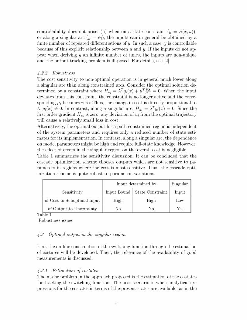
Table 1 summarizes the sensitivity discussion. It can be concluded that thecascade optimization scheme chooses outputs which are not sensitive to pa-rameters in regions where the cost is most sensitive. Thus, the cascade opti-mization scheme is quite robust to parametric variations.

Input determined by Singular

Sensitivity Input Bound State Constraint Input

of Cost to Suboptimal Input High High Low

of Output to Uncertainty No No YesTable 1Robustness issues

4.3 Optimal output in the singular region

First the on-line construction of the switching function through the estimationof costates will be developed. Then, the relevance of the availability of goodmeasurements is discussed.

4.3.1 Estimation of costates

The major problem in the approach proposed is the estimation of the costatesfor tracking the switching function. The best scenario is when analytical ex-pressions for the costates in terms of the present states are available, as in the

7

‘sweep method’ (λ = P x) used in the linear quadratic regulator. This is notthe case for the class of problems considered here.

Here, it is assumed that all the states are available. If full state measurementis not available, an appropriate state estimator needs to be set up. Considerthe case where all inputs are singular during the entire interval. An estimateλ(t) of λ(t) is obtained with the observer

˙λ(t) =−AT (x)λ(t)−G (λ(tf |t)− λ(tf |t)) (8)

A(x) =∂f

∂x(x) +

m∑i=1

∂gi∂x

(x)u∗i (9)

λ(tf |t) = T −1t,tf

(x) λ(t), λ(tf |t) =∂φ

∂x

∣∣∣∣∣x(tf |t)

(10)

Tt,tf (x) = e∫ tft

A(x(τ)) dτ , x(tf |t) = x∗(tf ) + Tt,tf (x(t)− x(t)∗) (11)

where x∗ and u∗i are the nominal state and input solutions to Problem (1) -(3). The estimated states x(tf |t) and costates λ(tf |t) at terminal time are pre-dicted using a state transition matrix, Tt,tf , to avoid having to repeat explicitintegration of the state and costate dynamic equations until final time at eachtime step. Note that the costate transition matrix is the inverse of the statetransition matrix. From the terminal states x(tf |t), the costates required forthe sake of optimality, λ(tf |t), are also calculated.

The gain matrix G is used to control the speed of correction. This is importantsince, if G = 0n×n, the λ trajectory deviates from its nominal value and thereis no guarantee that the final conditions on λ are met. Note that it is moreimportant to satisfy the final conditions on λ than the corresponding initialconditions. Thus, a closed-loop observer is proposed to force the costates atfinal time to their desired values.

The next complexity lies in the determination of Tt,tf (x). As a first approxi-mation, the nominal trajectory can be used to calculate the state transitionmatrix, i.e., Tt,tf (x) ≈ Tt,tf (x∗). In some cases, this is insufficient, and a first-

order Taylor series expansion can be used Tt,tf (x) ≈ Tt,tf (x∗) + (x− x∗)∂T∂x

.

When singular arcs are concatenated with other types of arcs, then predictionof the costates at final time becomes more involved. In such a case, the costatesat the end of the singular interval can be used instead of final time. The issuegets even more involved in the presence of state constraints, since the costatescan be discontinuous when entering or leaving the constraints.

4.3.2 Measurements

The costate estimation relies in general on full-state measurement which isnot always available. Also, some measurements may only be retrievable fromthe process with considerable delays. In such a case, the missing data maybe estimated with a suitable state estimator. However, as discussed above,the cost is rather insensitive to errors resulting from model or measurement

8

uncertainty along singular arcs. In the example section below, it will moreoverbe shown how the costate estimation scheme can be replaced by simple ad-hocadjustments of the singular input. Accurate full-state measurement is thus notessential in the singular case.

On the contrary, when process operation is limited by state constraints, it isessential to have accurate measurements or estimates of the states involvedin the constraint expressions as the process has to be operated as close aspossible to the constraints for optimal performance. Special instrumentationor algorithmic estimation efforts have to be provided in case of insufficientknowledge of this in general reduced set of states.

5 Conservatism to handle uncertainty

Here the feasibility of constraints in the presence of parametric uncertaintyand disturbance is considered next. The problem formulation is as follows:

minu(t)

Φ(x(tf )) (12)

s.t. x = f(x, θ) +m∑i=1

gi(x, θ)ui + d, x(0) = x0

S(x, u) ≤ 0

where d denotes a vector of randomly distributed process noise with zero meanand covariance vd. Assume that the disturbance is not correlated over time,i.e. E(d(τ) dT (τ ′)) = δ(τ − τ ′) diag(vd), where δ denotes the Dirac function.θ represents the set of uncertain parameters. The uncertainty description canbe either probabilistic or of the set membership type. In the former, θ isassociated with the probability distribution function p(θ), whilst in the latter,the only information available is θ ∈ Θ, where Θ is a bounded set. Note thatthe constraint expression does not explicitly depend on Θ: S(x, u) 6= S(x, u, θ).

5.1 Back-off calculations

The solution to the optimization problem (12) depends on the realization ofthe disturbance d and the value of θ, both of which are unknown. Thus, toensure feasibility of the path constraints despite the variations in d, back-offsfrom the constraints, which depend on the noise variance vd, have to be intro-duced. To calculate the back-offs amidst parametric uncertainty, two designvalues θ and vθ are necessary. They represent the mean and variance in thecase of probabilistic uncertainty description, θ = E[θ], vθ = E [(θ − E[θ])2 ] .When the uncertainty is of the set membership type, the worst case scenariois considered, θ = arg maxθ S(x(θ), u), vθ = 0.

9

The optimization then becomes:

Φb = minu(t)

Φ(x(tf )) (13)

s.t. x = f(x, θ) +m∑i=1

gi(x, θ)ui, x(0) = x0

S(x, u) + bS ≤ 0

The margins, or back-offs, bS are related to the uncertainty (disturbance andparametric errors) and will be calculated below. Note that the nominal solu-tion (x∗,u∗) to Problem (13) is obtained with the uncertainty being eliminatedfrom the system dynamics. The state evolution around the nominal trajectoryx∗ under the effect of uncertainty is considered via the back-offs in the pathconstraints. Since it has been assumed that d is zero-mean gaussian, Φb repre-sents, to a first-order approximation, the cost averaged over all the realizationsof d.The back-off expressions will now be derived. Let x(t) and u(t) denote theactual states and inputs of the system and ∆x(t) = x(t) − x∗(t), ∆u(t) =u(t) − u∗(t), ∆θ = θ − θ . The evolution of ∆x(t) can be calculated by thelinear time-varying state space model:

˙∆x(t) =A(t) ∆x(t) + B(t)∆u(t) + P (t)∆θ + d(t) (14)

A(t) =

(∂f

∂x+

m∑i=1

∂gi∂x

u∗i

) ∣∣∣∣∣x∗

(15)

B(t) = [g1 g2 · · · gm]∣∣∣x∗

P (t) =

(∂f

∂θ+

m∑i=1

∂gi∂θ

u∗i

) ∣∣∣∣∣x∗

(16)

Let the feedback provided by the cascade optimization structure be u = u∗ +ufb(y, y

∗, κ), where κ are the feedback controller parameters. The feedbackis analyzed in a neighbourhood of the nominal trajectory using the linearapproximation: ∆u(t) = −K(t) ∆x(t), where K(t) = −∂ufb

∂x. The variance of

∆x(t), vx = E[∆x(t) ∆x(t)T ], can be calculated as in [4] and reads:

vx(t) = vd

t∫0

Φ(τ) ΦT (τ) dτ + vθ

t∫0

Φ(τ) P (τ)P T (τ)Φ(τ) dτ (17)

where Φ(τ) = e∫ tτ

[A(t′) − B(t′) K(t′)]dt′ . The linearization of the constraintsgives:

S(x, u) = S(x∗(t), u∗(t)) +

(∂S

∂x− ∂S

∂uK(t)

)T∆x(t)

The back-off size is calculated such that feasible operation is ensured with theprobability α. For this, a factor β =

√2 erf−1(2α − 1) is introduced, where

erf−1 is the inverse error function of the normal distribution:

10

bS = β

(∣∣∣∣∣∂S∂x∣∣∣∣∣+

∣∣∣∣∣∂S∂u∣∣∣∣∣ |K(t)|

)T √diag(vx(t)) (18)

In practical applications, output measurements are also corrupted by noise:y = h(x, u) + η. Let the noise covariance matrix be vη. This can be taken

into account in the conservative design by replacing√diag(vx) by

√diag(vx)+√

diag(vη) in (18).

The back-offs needed in the open-loop case can be computed with (18) and set-ting K = 0m×n. Note that if the system matrix A(t) is unstable, the open-loopvariance of x may be large, requiring a lot of conservatism. The introductionof a feedback gain will stabilize the linearized system, thereby reducing vx. Al-ternatively, introduction of feedback increases

∣∣∣∂S∂u

∣∣∣ |K(t)|, which is zero in theopen-loop case. Feedback also introduces coupling between different inputs. Inthe process of reducing the back-off for Si, bSi , the back-off for Sj, bSj , mightbe increased. It is even possible that an inactive constraint Sj becomes activedue to an increase of bSj . Thus, a compromise between u∗(t) and K(t) has tobe sought in the solution to Problem (13).

5.2 Feedback design

The nominal input profile u∗(t) and feedback controller parameters κ are foundby solving the following optimization problem. Note that the back-offs bS givenby (18) implicitly depend on κ:

Φclb = min

u(t),κΦ(x(tf )) (19)

s.t. x = f(x, θ) +m∑i=1

gi(x, θ)ui, x(0) = x0

S(x, u) + bS ≤ 0

The following proposition is now formulated:

Theorem 2 Let Problem (13) be feasible and let there exists a κ such thatthe feedback ufb(y, y

∗, κ) = 0,∀y. Then the optimal cost Φclb of Problem (19)

is less than or equal to the optimal cost Φb of Problem (13).

Proof :

By choosing the κ which corresponds to ufb(y, y∗, κ) = 0,∀y, the feedback is

removed and Problems (13) and (19) are equivalent. Since it is assumed thatoptimization problem (13) is feasible, (19) also has a feasible solution. Due tothis inclusion, and since (19) has an additional degree of freedom, Φcl

b ≤ Φb.

QED

It has been observed that the sensitivity of the cost function with respect tothe parameters κ and the input vector u(t) are in general different. This leadsto conditioning problems in the numerical optimization. Therefore, instead ofsolving the optimization problem (19) which takes u(t) and κ simultaneously

11

as decision variables, it is preferable to solve it in an optimization structurewhere κ and u(t) are iterated in an inner-outer optimization structure:

minκ(t)

Φ(x(tf )

)= Φ

′(κ(t), u

)(20)

s.t. u(t) = argminu(t)

Φ(x(tf ))

x = f(x, Θ) +m∑i=1

gi(x, Θ)ui, x(0) = x0

S(x, u) + bS ≤ 0,

6 Case Study: Penicillin Fed-Batch Fermentation

In this section, the cascade optimization scheme is applied to the simulation ofa penicillin fed-batch fermentation process and is compared with both open-loop implementation and on-line optimization. Other biotechnology exampleshave been treated in [14,15].

6.1 Problem description

The kinetics of penicillin fermentation has been studied in [1]. These authorsproposed a simple model that is consistent with the observed functional depen-dencies of the specific growth rates, glucose uptake and penicillin formation,and estimated the model parameters to fit the experimental data. The modelcan be described as follows:

X =α(S,X) X − F X

V(21)

S=−α(S,X)X

Yx− θ(S)

X

Yp−Mx X + F

Sl − SV

(22)

P = θ(S) X −K P − F P

V(23)

V =F (24)

with F being the feed rate, Sl the feed concentration of the limiting substrate,X, S and P are the concentrations of biomass, substrate and penicillin respec-tively, and V the volume. A Contois law is used for the specific growth rateα(S,X) = αm S

S+Kl X. Yx and Yp are constant yield coefficients and Mx repre-

sents the cell maintenance term. The formation of penicillin is described by asubstrate inhibition model θ(S) = θm

1+KpS

+ SKi

and K is the first-order penicillin

decay rate. The model parameters are listed in Table 3. The model (21)-(24)presents a nonlinear affine-in-input structure with x = [X S P V ]T and u = F .

The operational constraints S ≤ Sm and X ≤ Xm are considered to avoidinduction of unwanted side reactions and for oxygen limitation respectively.

12

It is desirable to maximize the penicillin concentration for a given final time.The optimization problem reads thus:

minu(t)−P (tf ) (25)

s.t. x = f + gu, x(0) = x0

S − Sm ≤ 0, X −Xm ≤ 0

0 ≤ u ≤ um

The process parameters Yx and Sl are considered uncertain within the rangelisted in Table 4. Thus, the parameter uncertainty is of the set membershiptype. The nominal parameters (Table 3) are chosen in such a way that thesubstrate and biomass constraints will be satisfied for all possible combinationsof Yx and Sl when the nominal input is implemented on the process: θ =arg maxθ S(x(θ), u), vθ = 0.

The process is also perturbed by a random normally distributed disturbanced with standard variation σd = [0 0.02 0 0]T : x = f(x)+g(x)u+d. The distur-bance is physically motivated by additional fluctuations in the substrate inletflow. Additionally, it is supposed that full-state measurements are availableand, furthermore, are corrupted by normally distributed noise η with stan-dard deviation ση = [2 × 10−1 2 × 10−3 4 × 10−2 1]T . Note that full-statemeasurements are only required for tracking the switching function in thesingular region.

6.2 Nominal solution

Using Pontryagin’s Minimum Principle [3], it can be shown that the optimalsolution in fact consists of 6 arcs:

(i) an upper input bound arc for t ∈ [0 ts1];(ii) a substrate constraint arc for t ∈ [ts1 t

s2];

(iii) a lower input bound arc for t ∈ [ts2 ts3];

(iv) a biomass constraint arc for t ∈ [ts3 ts4];

(v) a singular arc for t ∈ [ts4 ts5];

(vi) a lower input bound arc for t ∈ [ts5 tf ].

The switching times are listed in Table 4. Some optimal trajectories and theswitching function are illustrated in Figure 3.

The optimal solution first lies on the upper input bound until the substrateconstraint S = Sm is reached. Then, it stays there in order to maximizethe biomass growth rate. Just before the biomass constraint is reached, thesubstrate level is lowered to the value Se for the following reason. When thebiomass constraint X = Xm is entered, it has to be tracked with the inputu = α(S,X) V (see equation (21) with X = 0). When such an input isapplied, it can be seen that the substrate dynamics (22) is unstable. To remainbounded, the biomass constraint has to be entered with the substrate value ofSe which corresponds to the equilibrium point of the internal dynamics. The

13

biomass constraint is exited again towards the end of the batch on a singulararc. A short arc with u = 0 terminates the batch since the final time cost issensitive to dilution.

Following the argument, it can be seen that the switching times ts1 to ts3 can bedetermined analytically, whilst ts4 and ts5 have to be determined numerically.The maximum penicillin concentration obtained with the set of parameterslisted in Table 3 is 8.23 g

l.

6.3 Open-loop implementation

In the presence of uncertainty, the open-loop input profile has to be designedand implemented with a certain conservatism in order not to violate the con-straints.

The back-offs are computed in the way exposed in Section 5 and using vθ = 0since the parametric uncertainty is of set membership type. The substrateand biomass profiles with the necessary back-offs can be seen in Figure 4 fordifferent parameter variations and disturbance realizations. Note the upperenvelope for the substrate uncertain evolution as predicted with formula (18).For the case of the nominal parameters YX = 0.47 1

hand Sl = 400g

l, the back-

off from the biomass constraint is very small due to fast and stable substratedynamics during this batch phase.

It is observed that the substrate concentration is considerably lower than Smwhich leads to a reduced growth rate. This causes a large loss in penicillinproductivity during the biomass constrained phase.

6.4 On-line optimization

A fine parametrization of the input was required during the initial batch phasesto model the sharp switching between constraints and to quickly correct theperturbed state profiles at the beginning of each reoptimization task. A piece-wise constant input parametrization with 80 elements was adopted for thetime interval t ∈ [0, 100] hours, whereas 20 elements were used on the remain-ing interval t ∈ [100, 150] hours. The optimization problem was solved using aSequential Quadratic Programming (SQP) routine in Matlab. The SQP rou-tine is time-consuming and frequently converged to a local minimum; thus, ithad to be restarted and manually guided to the optimal solution.

When the process is reoptimized, direct measurements of the process statesare used to estimate the uncertain parameters on-line. It is supposed thatthe inlet substrate concentration Sl can be measured and the yield factorYX determined from Yx = XV−X0V0

SlV−S0V0, under the assumption that most of the

substrate is indeed consumed by the biomass.

The back-offs can be reduced through on-line optimization since feedback isprovided by the reoptimization algorithm. Formulas (17) and (18) elaboratedin Section 5 can be suitably adapted for the back-off design along the substrate

14

constraint in this case. Indeed, at each reoptimization, the algorithm will at-tempt to bring the system back to the constraint if a deviation from S = Smoccurred. This feedback can then be modeled as the correction provided bya proportional controller ∆u(t) = −K(t) ∆x(t) which tracks the substrateconstraint. For a detailed derivation, see [14].

Since the back-off due to the disturbance is negligible along the biomass con-straint, no back-off from this constraint was used with this scheme. The per-formance of the on-line optimization scheme was found to be better the higherthe reoptimization frequency (see Table 2).

6.5 Cascade optimization with costate tracking

The proposed cascade optimization scheme was implemented in the followingmanner:

– When the input is on a bound (arcs (i),(iii) and (vi)), no feedback is applied.– A PI-controller tracks the substrate constraint in arc (ii). In arc (iv), a

controller (Figure 2) involving two cascaded PI controllers corrects any pos-sible offset from the biomass constraint and tracks the biomass at its upperbound. This structure was necessary to stabilize the substrate internal dy-namics and cope with the large time-scale differences between the biomassand substrate dynamics. Small back-offs from the state constraints are usedto cope with the noise effects. The sampling time is 5 minutes.

ProcessPI PI-

+

Se

X

X

SXm

-

+

S

F

Fig. 2. Biomass controller: Se is the off-line computed equilibrium value of theinternal dynamics

– The costate estimation scheme requires the computation of the final costate.As the final nonsingular arc is very short, the end of the singular arc isconsidered as the final time. The switching function was tracked with asuitably tuned PI-controller. No on-line parameter estimation is carried out.The G matrix in (8) is chosen in such a way that the costate estimationscheme is stable and the estimation transient fast.

– The switching instants ts1 to ts3 are adjusted on-line since they can be com-puted analytically. However, those switching instants which could not becharacterized analytically, i.e., the switching times ts4 to ts5 are left at theiroff-line computed values.

With the feedback design chosen, the back-offs for the cascade scheme wereconsiderably reduced in comparison to the open-loop case so that the substrate

15

and biomass could be tracked close to their constraints. This can be seen in thesimulations shown in Figure 5. The PI controller parameters for the substrateconstraint tracking were optimized iteratively. It was not necessary to optimizethe parameters for the cascade controller along the biomass constraint sincethe back-off given by the noise level was already very small. Note that theback-off is considerably reduced compared to the open-loop case (Figure 4).The switching function is tracked at its zero setpoint.

6.6 Cascade optimization without costate tracking

Note that in all batch phases apart from the singular arc, no parameter esti-mates and only partial state measurement are needed to achieve optimal per-formance. It was therefore investigated whether tracking the switching func-tion could be replaced by a simpler control strategy requiring no full-stateknowledge and parameter estimates.

From the off-line calculated optimal solution, it is seen that the input is con-tinuous as it enters the singular arc. Thus, the off-line computed singular inputalong with an additional offset is applied. The offset is adjusted to guaranteecontinuity. This adaptation of the input is expected to produce a good approx-imation of the singular input which maintains the substrate level to values forwhich the penicillin growth rate is optimal.

6.7 Performance comparison

Table 2 illustrates the average performance of the various implementationmethods for different parameter values. Note that the indicated costs corre-spond to average costs that are supposed to equal those obtained by solvingProblem (25) with the corresponding back-offs for each implementation case.

Yx Sl OL On-line opt. with no CO.co. CO.no. Ideal

2 4 64 150

0.43 360 7.14 7.55 7.87 7.91 7.94 7.94 7.91 7.95

0.47 360 7.43 7.75 7.91 7.94 7.99 7.99 7.98 8.00

0.45 380 7.67 7.91 7.95 8.07 8.09 8.09 8.09 8.10

0.43 400 7.89 8.04 8.14 8.17 8.18 8.19 8.18 8.20

0.47 400 8.19 8.19 8.19 8.21 8.22 8.22 8.22 8.23Table 2Performance comparison: OL = Open loop; no= number of optimizations; CO.co. =Cascade optimization with costate tracking; CO.no. = Cascade optimization with-out costate tracking; Ideal = Ideal solution with neither noise nor back-off

From any row in Table 2, the effect of back-offs on the average performancecan be observed. The back-offs are largest for the open loop case and are

16

reduced progressively with increasing reoptimization frequency. The smallestback-offs are obtained within the cascade optimization scheme. Thus, the av-erage performance augments from the open-loop implementation case to theon-line optimization scheme with increasing reoptimization frequency.

It is observed that a significant performance improvement is already obtainedwith a few reoptimizations. However, a total number of 150 optimizations, i.e.one reoptimization every hour, would be necessary to achieve the performanceof the cascade optimization scheme.

The benefit of cascade optimization over open-loop implementation is consid-erable. The improvement in performance is primarily achieved through reduc-tion of the offset from the biomass constraint.

When the cascade optimization strategy without costate tracking is consid-ered, the performance is only slightly lower than with the complete cascadeoptimization scheme. Consequently, the difficulties linked to the costate es-timation scheme can easily be avoided by a simple modification of the feed-back strategy. Hence, the cascade optimization scheme is able to achieve near-optimal performance despite model errors by using only a few state measure-ments.

The best performance for each parameter set was obtained by recomputingthe optimal solution with neither noise nor back-off. The performances of thecascade optimization scheme and on-line optimization with a total numberof 150 optimizations are very good and differ only insignificantly from theoptimal solution without back-off.

7 Conclusions

A cascade optimization scheme has been presented to implement an optimalsolution in the presence of uncertainty. The scheme relies on tracking appro-priate outputs during different time intervals. No feedback is applied whenan input is determined by its bound. The outputs to track are determinedfrom the state constraints when the optimal solution is determined by them.The switching function constitutes the optimal output when the solution issingular. Finally, feasibility of constraints is ensured despite uncertainty byintroducing margins from constraints.

The feedback scheme was applied to a simulated penicillin fed-batch fermen-tation process subject to disturbance and parameter variations. The optimalsolution was found and verified using Pontryagin’s Minimum Principle. Theperformance of the cascade optimization scheme was significantly superior tothat obtained by open-loop application of the off-line computed optimal so-lution. This was achieved by using only substrate and biomass measurementsand standard PI controllers. No numerical reoptimization or parameter esti-mation was required, making the performance of this scheme robust to modeland estimation errors.

Thus, the proposed cascade scheme constitutes a valuable improvement over

17

standard on-line optimization techniques by providing fast and robust feed-back which can be implemented in a well-instrumented industrial environment.Future research will focus on how to extend application of the proposed schemeto optimization problems involving terminal constraints.

Acknowledgements

The authors acknowledge the financial support of the Swiss National ScienceFoundation through the Project 21-46922.96.

References

[1] Bajpai, R.K., Reuss, R., Evaluation of Feeding Strategies in Carbon-Regulated Secondary Metabolite Production through Mathematical Modelling,Biotechnology and Bioengineering, Vol. 13, pp. 717-738, 1981.

[2] Baumann, T., Infinite Order Singularity in Terminal Cost Optimal Control:Application to Robotic Manipulators, Thesis No 1778, Ecole PolytechniqueFederale de Lausanne, Lausanne, 1998

[3] Bryson, A.E., Ho, Y.- C., Applied Optimal Control, Revised Printing,Hemisphere Publishing Corporation, New York, USA, 1975

[4] Chen, C.T., Linear System Theory and Design, Holt-Saunders, New York, 1970

[5] Eaton, J.W., Rawlings, J.B., Feedback Control of Nonlinear Processes usingOn-Line Optimization Techniques, Comp.Chem.Eng., Vol. 14, pp. 469-479,1990

[6] Kolavennu, N.S, Palanki, S., Cockburn, J.C., Nonlinear Controller Designby Uncovering Linear Dynamics Hidden by Input-Output Linearization,Proceedings ADCHEM 1997, pp. 511-516, Banff, 1997

[7] Krothapally, M., Palanki, S., A Neural Network Strategy for Batch ProcessOptimization, Comp.Chem.Eng., Vol. 21, pp. 463-468, 1997

[8] Palanki, S., Kravaris, C., Wang, H.Y., Synthesis of State Feedback Laws forEnd-Point Optimization in Batch Processes, Chem.Eng.Science, Vol. 48, 1, pp.135-152, 1993

[9] Robbins, H.M., A Generalized Legendre-Clebsch Condition for the SingularCases of Optimal Control, IBM Journal, pp. 361-372, July 1967

[10] Sampath, V., Palanki, S., Cockburn, J.C., Robust Nonlinear Control ofPolymethylmethacrylate Production in a Batch Reactor, Comp.Chem.Eng, Vol.22, pp. S451-S457, 1998

[11] Sastry, S., Bodson, M., Adaptive Control: Stability, Convergence andRobustness, Prentice-Hall, London, 1989

[12] Rawlings, J.B., Tutorial: Model Predictive Control Technology, Proceedings ofthe 1999 American Control Conference, Vol. 1, pp. 662-76, San Diego, 1999

18

[13] Srinivasan, B., Visser, E., Bonvin, D., Optimization-based Control withImposed Feedback Structures, Proceedings ADCHEM’97, pp. 635-640, Banff,1997

[14] Visser, E., A Feedback-based Implementation Scheme for Batch ProcessOptimization,, Thesis No 2097, Ecole Polytechnique Federale de Lausanne,Lausanne, 1999

[15] Visser, E., Srinivasan, B., Palanki, S., Bonvin, D., On-line Optimization ofBatch Processes by Tracking States and Costates, Proceedings IFAC WorldCongress, Vol. N, pp. 31-36, Beijing, 1999

19

0 50 100 1500

5

10

15

20

25

30

35

40Biomass (g/l)

Time (h)0 50 100 150

-0.1

0

0.1

0.2

0.3

0.4

0.5

0.6Substrate (g/l)

Time (h)

0 50 100 1500

2

4

6

8

10Flowrate (l/h)

Time (h)0 50 100 150

-0.2

0

0.2

0.4

0.6

0.8Switching function

Time (h)

Fig. 3. Optimal trajectories: analytical solution

0 50 100 1500

0.05

0.1

0.15

0.2

0.25

0.3

0.35

0.4

0.45

0.5

Substrate (g/l)

Time (h)

YX

= 0.43

S = 360l

YX

= 0.47

S = 400l

0 50 100 1500

5

10

15

20

25

30

35

40

Biomass (g/l)

Time (h)

YX

= 0.47

S = 400l

YX

= 0.43

S = 360l

Fig. 4. Biomass and substrate profiles with back-offs for various parameter valuesand disturbance realizations

20

0 50 100 1500

5

10

15

20

25

30

35

40

45

Biomass (g/l)

Time (h)0 50 100 150

-0.1

0

0.1

0.2

0.3

0.4

0.5

0.6Substrate (g/l)

Time (h)

0 50 100 1500

1

2

3

4

5

6

7

8

9

10Flowrate (l/h)

Time (h)

YX

= 0.43

S = 360l

YX

= 0.47

S = 400l

110 115 120 125 130 135 140 145 150-3.5

-3

-2.5

-2

-1.5

-1

-0.5

0

0.5

1x 10

-3Switching function

Time (h)

Fig. 5. Cascade optimization for various parameter values and disturbance realiza-tions: no numerical reoptimization

αm 0.11 1h Yx 0.47

Sl 400 gl Yp 1.2

Kl 0.006 Mx 0.029 1h

θm 0.004 1h Xm 40.0 g

l

Kp 0.0001 gl Sm 0.5 g

l

Ki 0.1 gl K 0.01 1

h

tf 150 h um 10 lh

Xo 1 gl Po 0 g

l

So 0.2 gl Vo 250 l

Table 3: Model parameters, operat-ing and initial conditions

ts1 0.019 h

ts2 40.897 h

ts3 40.997 h

ts4 113.467 h

ts5 149.998 h

Yx 0.43-0.47 1h

Sl 360-400 gl

Table 4: Off-line switching times andrange for parametric variations

21