Abstract— Railway control systems are largely based on data communication and network technologies. With the adoption of Ethernet-IP as the main technology for building end-to-end real-time networks on railway control systems, the requirement to deliver high availability, quality and secure services over Ethernet has become strategic. Critical real-time traffic is generally penalized and the maximum restoration time of 50 msec sometimes is exceeded because of real-time applications hangings, so passengers’ safety could be committed. It occurs on more than twenty percent of critical fail tests performed. Our main goal is to minimize restoration time from the application point of view. This article describes a protocol to improve critical real-time railway control systems. The algorithm designed gives us fast recoveries when railway computers fail down. The protocol permits to manage the railway control system from every computer in the network mixing unicast and multicast messages. Simulations obtained for a real railway line are shown. We have reached excellent results limiting critical failures recoveries to less than 50 msec.

Index terms—railway, critical systems, P2P architecture

A. INTRODUCTION Railway companies often have their own voice and

data communication infrastructure, usually based on SDH/PDH transmission systems over fiber or copper cables along the railway lines. This infrastructure supports general purpose and special computer services for railway traffic control and safety.

Only few years ago, railway systems were “islands” for traffic control and system safety, but now they are integrating network technologies, to permit easy growing, and central management.

With IP convergence, old serial communications via modem are migrating towards switched Ethernet networks over copper and fiber, with TCP/IP protocols.

New Critical or vital systems are based on Ethernet networks with physical ring topology, and fault tolerant procedures activated (such as Resilient Links, Fast Spanning Tree, HSRP o VRRP, routing protocols with load balancing capabilities, or redundant routes, and fast convergence such as EIGRP) [1].

Access networks are connected to regional nodes and different levels rings, to permit a central management of the systems. Regional networks usually are supported by SDH/PDH transmission systems, however, last trends in the core network points to MPLS/VPLS technology to implement VPNs and QoS [2].

We can distinguish two environments: Ethernet access networks with switches interconnected by dark fiber or xDSL links, and core network based on MPLS/VPLS

over SDH/PDH. The logical design in this networks is based on assign a separate VLAN for each application or real time traffic flow, establish a quality of service with level 2 or 3 marking, and make relationships between VLANs and VPNs at the core MPLS/VPLS network.

The main structure and technology for these networks respond basically to multimedia traffic requirements, but the behaviour is completely different when we are connecting critical real time systems to the same transport network. In fact, to avoid occasional blocking problems, is usual, to create two separate networks (one multiservice network to support non critical real time service and a second one to support critical real time services), These solutions increase complexity and difficult central management.

It is necessary to improve transport network to guarantee high quality communications. The main objectives of these improvements are three: minimize fail occurrences and get low recovery times (normally, lower than 50 milliseconds), guarantee quality of service to vital applications (also during the fail), and design network security to avoid unauthorized access.

Whereas the future on the network protocol seems to be decided for IP, there is no clear decision about the lower protocol layers (physical and data link access), which are the technological basis for today’s MAN and WAN backbone systems. To provide network fault resiliency, we can employ commercial level 1 methods based on physical redundancy (SDH/SONET), level 2 methods based on Ethernet common topologies (IEEE 802.1d, 802.1s, 802.1w, 802.3ad) or specific ring topologies (RPR/802.17 [3], EAPS/RFC3619 [4]) and level 3 methods based on routing protocols (EIGRP, ISIS, OSPF, BGP) and default-gateway backup protocols (VRRP, HSRP).

On the other hand, top levels of the communication architecture are implemented with proprietary protocols. There is no standard mechanism at these levels to obtain the necessary availability, reliability and safety ratios.

This paper is structured as follows. Section B describes components for railway control systems, how they work and their problems. Section C presents a protocol to solve railway control system problems, describes its messages and shows the fault-tolerant algorithms implemented. Simulations for a real railway topology are shown in Section D. Finally, Section E summarizes the conclusions and gives future works.

Jaime Lloret1, Francisco J. Sanchez2, Juan R. Diaz3 and Jose M. Jimenez4

A fault-tolerant protocol for railway control systems

Department of Communications, Polytechnic University of Valencia (Spain) 1jlloret@dcom.upv.es; 2jsbolumar@adif.es; 3jrdiaz@dcom.upv.es; 4jojiher@dcom.upv.es

B. RAILWAY TECHNOLOGY USED FOR CONTROL AND SAFETY

We can divide railway infrastructure technology in

control and safety technology. Control technology includes automatic train guidance, operating position representation and action tools in the event of deviations from the timetable. Safety technology or “signaling”, protects trains against collisions and derailment, using route protection (interlocking systems, block technology and level crossings) and train protection (monitoring the adherence to the permitted train speed). This article is focused on “signaling” systems, where RAMS (Reliability, Availability, Maintainability, and Safety) factors become critical for achieving the required overall passenger safety.

When a safety component fails, the affected system must revert to a non-dangerous (safe) state, to match with the fail-safe principle: signal sets to stop in the event of a fault in the interlocking system, switch maintains its position if a fault occurs in the interlocking system, etc.

Computers are not considered systems with intrinsic safety, and then it is necessary duplicate hardware. A dual-channel computer command system for the green lamp of a rail signal (see figure 1) is a simple example. In this example, the dual-computer system, which controls the lamp and performs a monitoring function (not shown in figure 1 for simplicity) is commanded by a single-channel, secure data transmission channel. This also serves in the rearward direction as a transmission channel for forwarding the “actual” state of the lamp (on/off/disturbed) to the secure central computer of the interlocking system. Really, for costs reasons, a dual-computer system controls and monitors several signals in parallel. This solution is enough to guarantee safety operation, but does not offer high availability and true fail-safe. Therefore, all signaling systems must be designed to “fail-safe”, adding an additional computer in “two-out-of-three” scheme, but, this model is not applied at normal stations for saving economic costs.

In the communication protocol stack for vital signaling and control applications, the lowest layers (physical layer and basic transport functions) are covered by commercially available components (network interface cards with communication software), for example, Ethernet with User Datagram Protocol (UDP) or field busses (such as Profibus or Controller Area Network bus) and communication loops (RS-232, RS-422, RS-485 and so on). Above these two layers are the fail-safe functions: connection supporting functions, safety-related functions and proprietary applications.

The most critical signaling systems are railway station interlocking systems (shown in figure 2), usually

composed by objects (sensors/actuators or input/output devices) installed on the track (signals, track circuits and so on), controller objects to manage several objects, concentrators for attending communications from controller objects, and finally, two or three redundant computers or CPUs that collect data and maintain station object database. Device connections are often based on Ethernet, or formerly on field buses and communication loops. Figure 3 shows a detailed functional diagram of railway station interlocking system. CPUs are continuously checking vital parts and components (track circuits, point motors, etc.) and non-vital parts (local control, centralized traffic control, etc.). In case of vital parts failure, all signals become red and the train is stopped, until service restoration by human interaction.

A real example of a complete railway control system network is shown in figure 4. Circles represent routers in each station interlocking system, rectangles represent switches using HSRP protocol and squares represent interlocking CPUs. Dotted lines are the backup network lines.

If a hardware component breaks down, an operating restriction would be created, and the staff must assume the responsibility for the safe working of the system, based on prescribed operating instructions. Several hours may elapse until the defective component is repaired. During this time, the risk of an accident increases substantially comparing direct human intervention with normal automatic operation. If the fail affects an object controller, only the controlled objects will be not in operational state, and is still possible maintain a minimum degraded functionality.

Generally, CPUs are the only redundant components. Theoretically, when a CPU fails down, a backup CPU must take control of the program in real-time, but unfortunately sometimes the switching sequence does not performed (specially when train traffic density is high or a log audit process is running) and complete hanging is caused: there is no communication with object controllers and block function with other stations is inoperative. For restore normal operation we must spend since several minutes (basic functions) to close to an hour (all functions). According to this, we can identify two main problems: first one, about CPU load balancing, and second one, about fault tolerance and service restoration.

C. PROTOCOL DESCRIPTION

Our purpose is to connect computers forming different

groups, in order to transmit sensor data and to provide data redundancy in the network, so if a computer fails, sensor data could be collected from computers from other groups.

Figure 1. Dual-channel computer control system for the green lamp

of a railway signal.

Figure 2. General view of railway station interlocking system.

Figure 3. Functional diagram for interlocking system.

Figure 4. Railway line control system network topology.

We have designed a scalable protocol because new computers and sensors could be needed in the network. The protocol used by computers to collect data from the sensors use to be private, so, the protocol created does not have to be dependent on particular manufacturers’ protocol and it has to work in conjunction with them using an additional service. The interconnection system overload issue needs to be addressed avoiding so many messages and using load balancing.

In order to create the protocol, we have divided railway stations in groups as it is shown in figure 4. Each group has a set of computers managing the sensors of the railway station. All computers, which collect data from the sensors, have to run the proposed protocol.

Technical people use technical support computers to control the state of sensors of the station. These computers will be able to access to all data collected from all redundant computers, but they will not need to run the algorithm described below, they will act just as a desktop client. From now, we are not going to consider these computers because the protocol runs without them.

1st. System components and parameters

The proposed interconnection system is divided in

three layers: - Organization layer: Computers in this layer organize

connections between computers from different

groups. One computer of each group makes it up. This computer acts as a representation of the other computers. We call this computer “primary”. Primary computers must have connections with primary computers from other groups.

- Distribution layer: Each group has its distribution layer, made up by all its computers. From now we are going to call to each one of them “secondary”. Each secondary computer has a connection with the primary computer in its group and connections with one secondary computer from every group as a hub-and-spoke. These connections allow sharing sensor data information between groups.

- Access layer: Technical support computers make it up.

A primary computer has organization and distribution layer functionalities, but secondary computers only have distribution layer functionalities.

Figure 5 shows the system described. One secondary computer has only connections with other secondary computers from other groups.

The backup computer is a secondary one, but it is the primary computer’s designated successor, so it keeps its information as a secondary computer and the same information of the primary computer. In case of primary computer failure, it will become primary computer and a new backup computer will be elected. The primary computer, as a function of secondary computer’s

Serial input: CRC code protection appendix, dual transmission, sequentil number, etc.

Computer channel 1

Computer channel 2

Computer - Computer connection

CRC: Cyclic Redundancy Check

220 V Green lamp

Secure 2-channel computer system (2-out-of-3 system)

Station 1 Station 2 Station 4Station 3

Station 5 Station 6 Station 7 Station 8

Train Management System, TMS

IInntteerrlloocckkiinngg CCPPUUss

Object Controllers Rail-yard

Concentrators

Transmission Loops

LAMPSOUTPUT

RELAYSOUTPUT

VITALINPUTS

NON VITAL

COMMUN.

CPUS

VITAL CONTINUOS COMMUN.

DIAGNOSTIC

REMOTECONTRO

IN OUT

TRFS

TRANSPATP

GENATP

Remote Control

ON/OFFSIGNALS

INTERLOCKRELAYS.

POINTMOTOR

TRACK CIRCUITS

INTERLOCK RELAYS

(1) COMMUNICATIONS WITH NEXT STATION. (2) COMMUNICATIONS WITH ANOTHER INTERLOCKING IN

ALFAFA

AUDIT TERMINAL TO STORE ACTIVITY LOGS

AND REPLAY EVENTS

VITAL CONTINUOS COMMUN.

MANAGEMENTTERMINAL.

CONTAC

ATPINTERFACE

available connections and the load they can support, takes the backup computer election. From now, the backup computer will be considered as a secondary one.

Every computer in the organization and distribution layers needs the following information: - GroupID. It is a unique 16-bit identifier indicating to

which group the computer is joined. Every group has one groupID and every new computer in the architecture has to choose it from its startup.

- NodeID. It is a 16-bit identifier indicating the number of the computer in the group. It is unique for each computer. The primary computer will have the first one and, then, assigns it sequentially when a computer joins the group. If a computer fails down, when it joins the network again, primary computer will assign last available nodeID to it.

- Max_Con: It is the maximum number of connections the computer supports from other computers.

- Max_Load: It is the maximum load the computer can carry out.

- Upstream and Downstream Bandwidth in Mbps. Max_Con value can be expressed using expression 1.

∑∑−

=

−

=

+=1

1

1

1_

n

j

g

ijiConMax (1)

Where g is the number of groups in the network and n

is the number of computers in its group. In case of a primary computer, the more computers are in a group lower connections available are for other primary computers. In case of a secondary computer, it uses only one connection for its primary computer and the rest are available. Considering every station in figure 4 as a group and Max_Con≥13, primary and secondary computers’ connections are shown in figure 6.

We have defined P parameter in order to know which computer is the best computer to promote and to be primary one. It depends on the computer upstream and downstream bandwidth and its stability in the group. We have considered that computers with higher bandwidth and more stable are preferred (in case of equal bandwidth, the most stable ones are preferred). Expression 2 is the one that fits best the P parameter.

( ) ( )( ) 12log16 KnodeIDBWBWP downup ⋅−++= (2)

K1 emphasizes bandwidth part. We have chosen a

value of 200 by default, but it can be changed. Computer upstream and downstream bandwidth is 10 Mbps, 100 Mbps and 1 Gbps. Figure 7 shows P parameter as a function of computers’ bandwidth. We can see that computers with log2(nodeID) values lower than 10 are preferred.

In order to know which is the best computer to have connections with, we have defined C parameter. It gives us the computer’s capacity and depends on its upstream and downstream bandwidth (in Kbps), its available number of connections with other computers, its maximum number of connections and its % of available load. C parameter is defined by expression 3.

( )

ConMaxKloadConAvailableBWBW

C downup

_100_)·(log 22 +−⋅+

= (3)

Where 0 ≤ Available_Con ≤ Max_Con. Load varies

from 0 to 100. A load of 100% indicates the node is overloaded. K2 give us C values different from 0 in case of a load of 100% or Available_Con=0. We have chosen K2=1 to get C into desired values. Figure 8 shows C values as a function of computers’ available connections. We have fixed node’s load to 85%.

Computer’s topology is different according to the layer where they are placed. Next sections describe organization and distribution layer computer operations.

2nd. Organization layer operation

There is only one primary computer per group and all

primary computers make up the organization layer. Primary computers must have a groupID and must

authenticate with primary computers from other groups previously known or by bootstrapping [5]. They establish that connections using “P connect” messages. Although each one has established a connection with the others, they must open a multicast address to receive keepalive messages (we have chosen 231.0.0.1). Every 10 milliseconds, primary computers send a keepalive message to that multicast address containing its groupID, its nodeID, and its C parameter.

Primary computers build two types of tables: the primary computers’ neighbour table and the access table.

The primary computers’ neighbour table is used to connect primary computers. Every primary computer has one with all its neighbours. This information is obtained through keepalive messages from other primary computers. Table 1 shows registers for one entry. Hold time is three times keepalive time, so when a computer does not receive a keepalive message for a 30 milliseconds, this entry has failed.

Primary computer sends only primary’s neighbour table to the backup computer using the “backup” message when changes take place (incremental updates).

In a small network primary computers’ neighbour table will have all primary computers in the network, so the topology will be a full-mesh, but in case of many groups, we propose the use of Short Path First algorithm for primary computer topology as it is explained in [6].

Figure 5. System layers.

02468

101214

Primary Station1

Primary Station2

Primary Station3, 4, 8

Primary Station5, 6, 7

Secondary

Computers

Used Connections

Other groupsIts group

Figure 6. Figure 4 primary and secondary computers’ connections.

0500

1000

15002000

2500300035004000

45005000

5500

0 4 8 12 16nodeID

P 10 Mbps 100 Mbps 1 Gbps

Figure 7. P as a function of computers’ bandwidth.

0

20

40

60

80

100

120

140

160

180

0 2 4 6 8 10 12 14 16Available_Con

C 10 Mbps 100 Mbps 1 Gbps

Figure 8. C as a function of computers’ available connections.

1st GroupID 2nd NodeID 3rd Network Address 4th Keepalive Time 5th Hold Time 6th C parameter 7th Backup nodeID 8th Backup Network Address

Table 1. Primary computers’ neighbour table.

All computers in the same group make up the access table. It is used to know online computers in the group and to send information when secondary nodes from other networks request it. When a new computer joins the group using a “S connect” message, the primary computer assigns it a nodeID, using a “nodeID” message, and adds it to the access table. Then, the secondary computer has to send it a keepalive message every 10 milliseconds. The keepalive contains its groupID, its nodeID, the keepalive time and the hold time, its P parameter and its C parameter. The computer with higher P value will be the backup computer. Table 2 shows registers for one entry.

First register will be the primary computer and the second registry will be the backup computer.

Secondary computers open a multicast address to receive multicast messages from the primary computer. We have chosen 230.0.0.0 as the start multicast address. Last 16 bits will be the groupID. Primary computers send secondary computers the access table through that multicast address using the “AT” message. It is sent using incremental updates when changes take place.

3rd. Distribution layer operation

Every new computer will authenticate with the

primary computer in its group previously known or by

bootstrapping [5]. They establish connections with primary computers using “S connect” messages. The connection is used to know which computers are in its group and to request neighbours from other groups.

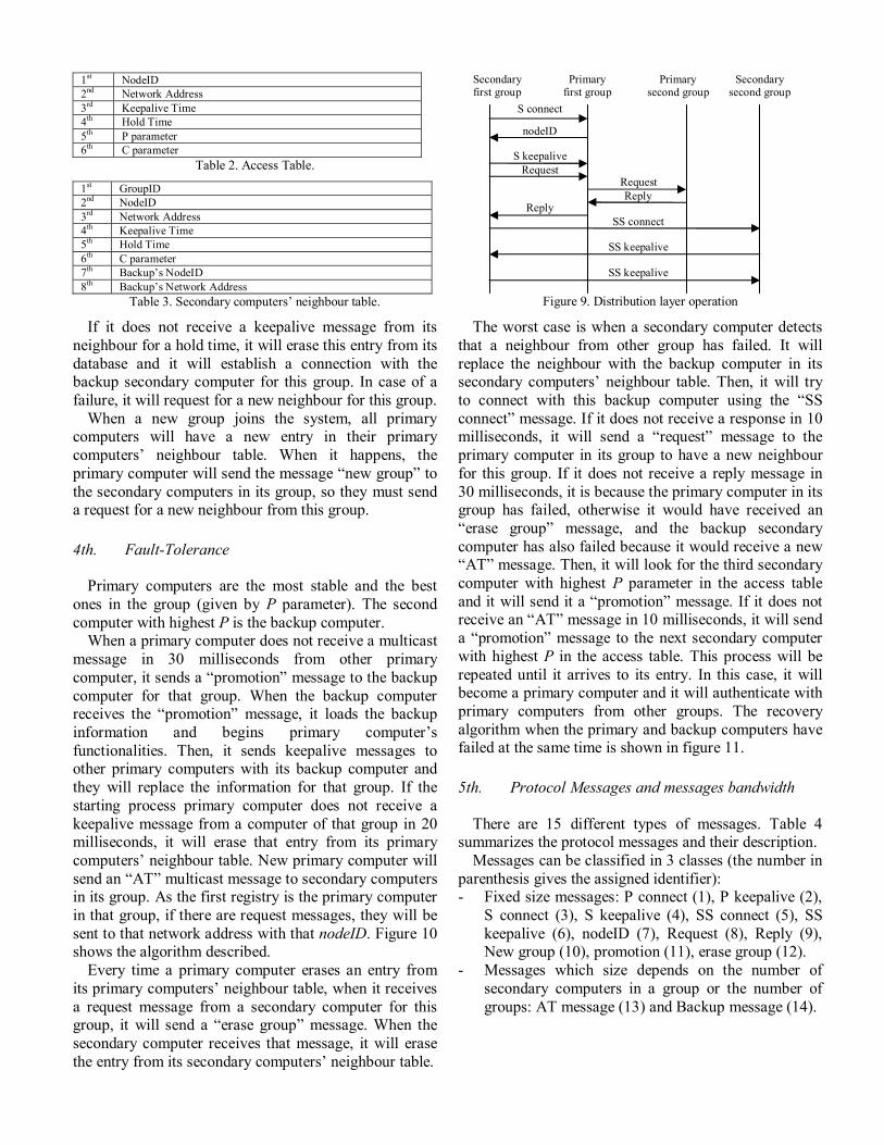
Secondary computers have to send sensor data to other groups to replicate their information. In order to know which secondary computers are the best ones to have connections with, a secondary computer has to send a “request” message to the primary computer in its group. This message contains the destination groupID (if it is the first time it sends this requesting message, groupID will be 0xFF indicating all groups). This primary computer will forward this request to the destination (unicast address in case of one destination and multicast address in case of all groups). Primary computer from second group will choose 2 highest C parameter second computers in its access table and it will reply with the “reply” message which has its groupID and their nodeID and network address to the primary computer from the first group. Primary computer from the first group will forward this reply to the requesting secondary computer. The second computer from the first group sends a “SS connect” message to its new neighbour and adds the secondary computer whit highest C parameter as the first entry for this group and the second one as a backup. The backup secondary computer is used in case of the first one failure. If both secondary computers fail, the process will begin again. Then, secondary computers can send sensor data to their neighbour using “D” messages. Steps explained are shown in figure 9.

All entries will be added to the secondary computers’ neighbour table (it is shown in table 3). A secondary computer must send keepalive messages to its neighbours every 10 milliseconds. The keepalive contains its groupID, its nodeID, and its C parameter.

Distribution Layer

Access Layer

Primary Backup Technical SupportSecondary

Group 1

Group 2

Group 3

Organization Layer

1st NodeID 2nd Network Address 3rd Keepalive Time 4th Hold Time 5th P parameter 6th C parameter

Table 2. Access Table.

1st GroupID 2nd NodeID 3rd Network Address 4th Keepalive Time 5th Hold Time 6th C parameter 7th Backup’s NodeID 8th Backup’s Network Address

Table 3. Secondary computers’ neighbour table.

Figure 9. Distribution layer operation

If it does not receive a keepalive message from its neighbour for a hold time, it will erase this entry from its database and it will establish a connection with the backup secondary computer for this group. In case of a failure, it will request for a new neighbour for this group.

When a new group joins the system, all primary computers will have a new entry in their primary computers’ neighbour table. When it happens, the primary computer will send the message “new group” to the secondary computers in its group, so they must send a request for a new neighbour from this group.

4th. Fault-Tolerance

Primary computers are the most stable and the best

ones in the group (given by P parameter). The second computer with highest P is the backup computer.

When a primary computer does not receive a multicast message in 30 milliseconds from other primary computer, it sends a “promotion” message to the backup computer for that group. When the backup computer receives the “promotion” message, it loads the backup information and begins primary computer’s functionalities. Then, it sends keepalive messages to other primary computers with its backup computer and they will replace the information for that group. If the starting process primary computer does not receive a keepalive message from a computer of that group in 20 milliseconds, it will erase that entry from its primary computers’ neighbour table. New primary computer will send an “AT” multicast message to secondary computers in its group. As the first registry is the primary computer in that group, if there are request messages, they will be sent to that network address with that nodeID. Figure 10 shows the algorithm described.

Every time a primary computer erases an entry from its primary computers’ neighbour table, when it receives a request message from a secondary computer for this group, it will send a “erase group” message. When the secondary computer receives that message, it will erase the entry from its secondary computers’ neighbour table.

The worst case is when a secondary computer detects that a neighbour from other group has failed. It will replace the neighbour with the backup computer in its secondary computers’ neighbour table. Then, it will try to connect with this backup computer using the “SS connect” message. If it does not receive a response in 10 milliseconds, it will send a “request” message to the primary computer in its group to have a new neighbour for this group. If it does not receive a reply message in 30 milliseconds, it is because the primary computer in its group has failed, otherwise it would have received an “erase group” message, and the backup secondary computer has also failed because it would receive a new “AT” message. Then, it will look for the third secondary computer with highest P parameter in the access table and it will send it a “promotion” message. If it does not receive an “AT” message in 10 milliseconds, it will send a “promotion” message to the next secondary computer with highest P in the access table. This process will be repeated until it arrives to its entry. In this case, it will become a primary computer and it will authenticate with primary computers from other groups. The recovery algorithm when the primary and backup computers have failed at the same time is shown in figure 11.

5th. Protocol Messages and messages bandwidth

There are 15 different types of messages. Table 4

summarizes the protocol messages and their description. Messages can be classified in 3 classes (the number in

parenthesis gives the assigned identifier): - Fixed size messages: P connect (1), P keepalive (2),

S connect (3), S keepalive (4), SS connect (5), SS keepalive (6), nodeID (7), Request (8), Reply (9), New group (10), promotion (11), erase group (12).

- Messages which size depends on the number of secondary computers in a group or the number of groups: AT message (13) and Backup message (14).

S connect

Secondary first group

Primary first group

Primary second group

Secondary second group

nodeID

S keepalive Request

Request Reply

Reply SS connect

SS keepalive

SS keepalive

Figure 10. Recovery algorithm for primary computers.

Figure 11. Recovery algorithm for primary computers when the

primary computer and the backup fail at the same time.

Name Type Description P connect Unicast Primary computers send that message to establish connections with primary computers from other groups. It has its groupID, its

nodeID and its C parameter. P keepalive Multicast It is a message between primary computers. It has the groupID of sender’s group, nodeID, keepalive time, hold time, C parameter and

the nodeID and network address of its backup computer. Its information updates primary computers’ neighbour table. S connect Unicast Secondary computers send that message to establish a connection with the primary computer from its group. It has its groupID. nodeID Unicast Primary computers send that message to the new secondary computer. It has its groupID and the assigned nodeID. S keepalive Unicast Secondary computers send that message to the primary computer in its group. It has the groupID, nodeID, keepalive time, hold time, P

parameter and C parameter. SS connect Unicast Secondary computers send that message to establish a connection with the secondary computer from the other group. It has its

groupID, nodeID and C parameter. SS keepalive Unicast Secondary computers send that message to the neighbour secondary computers from other groups. It has the groupID, nodeID,

keepalive time, hold time and C parameter. AT Multicast Primary computers send its access table to all nodes in its group. First message has its groupID and the nodeID, network address, P

and C parameters of all computers in the group. Next messages have only information related with new secondary computers. Backup Unicast Primary computers send this message to the backup computer. First message has the groupID, nodeID, network address and C

parameter of all primary computers in the network. Next messages have only information related with new primary computers. Request Unicast/

multicast They are messages from secondary computers to request secondary computers adjacencies. Primary computer forwards this request to some (or all) primary computers its primary computers’ neighbour table based on the destination. They have the destination groupID, the requesting computer groupID and its nodeID.

Reply Unicast They are messages from primary computers as a reply of a request message from secondary computers from other groups. They are used to build the secondary computers’ neighbour table. They have the requesting groupID and nodeID and the groupID, nodeID and the network address of the chosen secondary computer.

New group Multicast Primary computers send this message to their secondary computers every time there is a new group in the network. This message has new group’s groupID.

Promotion Unicast This message is sent from a primary computer, that detects a primary computer from other group has failed, or a secondary computer, that detects its primary computer has failed, to the backup computer or other secondary computers in that group. It has its groupID.

Erase group Unicast This message is sent from the primary computer that has sent a request message for a group that has failed, to the secondary computers. It has the groupID to be deleted from its secondary computers’ neighbour table.

D Unicast They are messages between secondary computers of different groups. They are used to send sensor data between groups. Table 4. Protocol messages

- Messages which size depends on the sensor data transferred: D message (15).

Taking into account the number of bits used for each field (shown in table 5), data messages from sensors have 64 bytes and message sizes are based on Ethernet and TCP/IP headers (the sum of these headers is 58 bytes as it has been considered for other P2P protocols [7]). Bandwidth cost in bytes for each message, when there are 8 groups and each one with 8 computers, is shown in figure 12. We can see that all messages are lower than the limit size of the payload for TCP/IP over Ethernet, so they will fit in one message and they will not be split.

D. SIMULATIONS We have simulated the topology shown in figure 4.

The time needed to send a 65 Bytes message to the medium (transmission delay) is lower than 120 µseconds. We have considered that the time needed to compute (processing delay) an average message is around 600 µseconds. Propagation time varies as a function of the distances between stations and the propagation delays through intervening network components (switches and routers). Distances between stations are 1 Km. The propagation delay is 10 µsecs.

Check keepalive times for other primary computers

Update the primary computers’ neighbour

table using the keepalive message

Yes

No

Yes No

Erase this entry from the primary

computers’ neighbour table

¿Is there any keepalive message for that group

before 20 msec?

Send a promotion message to the backup computer for that group

¿Is there any keealive time higher than the hold time (30 msec)?

Update the secondary

computers’ neighbour table

¿Is there any keealive time higher than the hold time (30 msec)?

Yes

No

¿Is there a keepalive message from that computer before 10

msec?

Yes

No

Check keepalive times for neighbours in its secondary computers’ neighbour table

Send a “SS connect” message to the backup secondary computer for this group

¿Is there a reply before 30 msec?

Send a request message for that group

Update the secondary

computers’ neighbour table

Yes Look for the next secondary computer with highest P parameter and send it a “promotion”message

No

¿Is there a new “AT” message before 10 msec

or I am the next?

No

Yes, there is an “AT” message

Become a primary computer and send

“P connect” messages

Yes, I am the next one

Field Bits Number of messages 8 groupID 16 nodeID 16 P parameter 16 C parameter 16 Keepalive time 4 Hold time 4

Table 5. Bits cost for messages’ fields. Bytes

0

20

40

60

80

100

120

140

160

180

1 2 3 4 5 6 7 8 9 10 11 12 13 14 15 Figure 12. Bandwidth cost for each message.

Physical layer and Data link layer failures are usually recovered by lower protocols such as HSRP protocol (as it can be read in [1]). We do not consider this type of failures because we focus our research on computer data recovery.

Figure 13 shows the simulations obtained using the Network Simulator-2 [8]. In t=-20 msecs. the system is stable and it works correctly. Back line shows the number of bits per msecs. in the network when a primary computer fails down in t=0 msec. In this case, the failed computer sent a keepalive message in t=-5 msecs. When t=25 msecs, all primary nodes from other groups send a keepalive message to the backup computer for that group. Then, the secondary computer becomes primary computer and, in t=32 msecs, sends AT messages to secondary nodes in its group. Finally, the system converges. Grey line shows the number of bits per msecs in the network when a secondary computer sends a request message and finds that the primary computer and the backup computer have failed at the same time. In this case, in t=0 msecs, the secondary computer sends a “request” message to the primary in its group in order to have an adjacency with a secondary computer from a group which does not have adjacencies with it. In t=30 msecs expires the time to have a reply, so the primary or the secondary computer in its group has failed, so it sends, in t=40 msecs, a “promotion” message to the third secondary computer in the access table. It is no reply, so it sends a “promotion” message to the fourth secondary computers in its group. The fourth secondary computer is alive, so it becomes a primary computer and sends an “AT” message to the secondary computers in the group.

Both simulations show us how many packets are exchanged between nodes. Finally, we have checked that all nodes have the correct adjacencies, so the recovery algorithm is faster than 50 msecs.

2000

3000

4000

5000

6000

7000

8000

-20 -10 0 10 20 30 40 50 60 70msec

Bits Primary Computer Failure Primay & Backup Computer Failre

Figure 13. Simulations for the protocol proposed in a real topology.

E. CONCLUSIONS This paper has described a fault-tolerant protocol for

railway control systems that allows topology changes. Connections between computers are based on computers’ capacity, so every computer sends its sensor data to the most capable computers in the network to provide redundancy. Algorithms implemented converge in less than 50 milliseconds to provide real-time recoveries. The protocol mixes unicast and multicast messages to decrease the bandwidth used. Although, we have defined some parameters (such as nodeID and C and P parameters) to have an autonomous system, the railway technicians could manage them manually.

Future works will use this protocol to contrast sensor data from different manufacturer sensors. Security and data integrity will also be implemented.

References

[1] Francisco J. Sánchez, Jaime Lloret, Juan R. Díaz, José M. Jiménez “Mecanismos de protección y recuperación en redes de tiempo real para el soporte de servicios de explotación ferroviaria”, XX Simposium Nacional de la Unión Científica Internacional de Radio (URSI’05), September 2005. [2] VPLS IETF drafts: http://www.ietf.org/internet-drafts/draft-ietf-ppvpn-vpls-requirements-01.txt [3] IEEE 802.17 Resilient Packet Ring Working Group: http://www.ieee802.org/17/ [4] RFC3619 “Ethernet Automatic Protection Switching”: http://www.faqs.org/rfcs/rfc3619.html [5] C. Cramer, K. Kutzner, and T. Fuhrmann. “Bootstrapping Locality-Aware P2P Networks”. The IEEE International Conference on Networks, Vol. 1. Pp. 357-361. 2004. [6] J. Lloret, F. Boronat, C. Palau, M. Esteve, “Two Levels SPF-Based System to Interconnect Partially Decentralized P2P File Sharing Networks”, International Conference on Autonomic and Autonomous Systems International Conference on Networking and Services, October 2005. [7] Beverly Yang and Hector Garcia-Molina. Improving Search in Peer-to-Peer Networks. Proceedings of the 22nd International Conf. on Distributed Computing Systems, 2002. [8] McCanne and S. Floyd, “ns-Network Simulator”. At http://wwwmash. cs.berkeley.edu/ns/, 1995.