A Discrete Variable Chain Graph for Applicants for CreditAuthor(s): E. Stanghellini, K. J. McConway and D. J. HandSource: Journal of the Royal Statistical Society. Series C (Applied Statistics), Vol. 48, No. 2(1999), pp. 239-251Published by: Wiley for the Royal Statistical SocietyStable URL: http://www.jstor.org/stable/2680800 .

Accessed: 07/02/2015 09:50

Your use of the JSTOR archive indicates your acceptance of the Terms & Conditions of Use, available at .http://www.jstor.org/page/info/about/policies/terms.jsp

.JSTOR is a not-for-profit service that helps scholars, researchers, and students discover, use, and build upon a wide range ofcontent in a trusted digital archive. We use information technology and tools to increase productivity and facilitate new formsof scholarship. For more information about JSTOR, please contact support@jstor.org.

.

Wiley and Royal Statistical Society are collaborating with JSTOR to digitize, preserve and extend access toJournal of the Royal Statistical Society. Series C (Applied Statistics).

http://www.jstor.org

This content downloaded from 141.250.1.55 on Sat, 7 Feb 2015 09:50:03 AMAll use subject to JSTOR Terms and Conditions

Appl. Statist. (1999) 48, Part 2, pp. 239-251

A discrete variable chain graph for applicants for credit

E. Stanghellini Universita di Perugia, Italy

and K. J. McConway and D. J. Hand The Open University, Milton Keynes, UK

[Received October 1996. Final revision June 1998]

Summary. A bank offering unsecured personal loans may be interested in several related outcome variables, including defaulting on the repayments, early repayment or failing to take up an offered loan. Current predictive models used by banks typically consider such variables individually. However, the fact that they are related to each other, and to many interrelated potential predictor variables, suggests that graphical models may provide an attractive alternative solution. We developed such a model for a data set of 15 variables measured on a set of 14000 applications for unsecured personal loans. The resulting global model of behaviour enabled us to identify several previously unsuspected relationships of considerable interest to the bank. For example, we dis- covered important but obscure relationships between taking out insurance, prior delinquency with a credit card and delinquency with the loan.

Keywords: Chain graphs; Conditional independence models; Credit scoring; Finance

1. Introduction

Over the last year, British consumers borrowed about ?500 billion. This came from various sources, including credit cards, mortgages and banks. Of these, the largest chunk, about 60%, was provided by High Street banks. To obtain credit, the typical applicant completed an application form, giving relevant details of financial affairs and demographic characteristics. Originally, this information would have been analysed by using human judgment to decide to whom credit should be granted. However, in response to the growth in demand, and facilitated by the opportunities provided by dramatic increases in computer power, formal statistical methods are now employed to yield a prediction of the risk that an applicant will default on the repayments. Methods used for formulating the prediction rule include simple linear regression, logistic regression, classical discriminant analysis and nonparametric discrim- ination techniques such as nearest neighbour methods and recursive partitioning methods. More recently, neural networks and genetic algorithms have been explored, though they have yet to see adoption in real day-to-day implementations. Details of work in the area are given in Rosenberg and Gleit (1994), Hand and Henley (1997), Hand and Jacka (1998) and the references cited therein. Collections of papers on credit scoring and credit control can

Addrl-ess for correspondence: D. J. Hand, Department of Statistics, The Open University, Walton Hall, Milton Keynes, MK7 6AA, UK. E-mail: d.j.hand@open.ac.uk

( 1999 Royal Statistical Society 0035-9254/99/48239

This content downloaded from 141.250.1.55 on Sat, 7 Feb 2015 09:50:03 AMAll use subject to JSTOR Terms and Conditions

240 E. Stanghellini, K J. McConway and D. J. Hand

be found in occasional issues of the IMA Jourzcnal of Mathematics Applied in Butsiness anid Industry as well as in Thomas et al. (1992).

For a simple classification into a restricted number of clearly defined classes, such methods can be highly effective. However, they have limitations. In particular, they assume that the criterion variable is selected beforehand, that the classes are well defined, that one is never interested in and never will be interested in - anything else and that the banking environ- ment is static. Sometimes these assumptions are appropriate hence the success of supervised classification methods in the past. But often they are less appropriate: new financial products are constantly being developed, customers want new kinds of services and the banking environ- ment is increasingly competitive. In any case, as we shall see, there are many different aspects of customer behaviour that the bank may be interested in predicting. It would also be useful if the model could be used 'in reverse': instead of looking at an applicant's characteristics and predicting their behaviour, we would like to be able to specify desirable behaviour and to identify the characteristics of people who are likely to behave in that way. The complexity and interrelated nature of all of this suggests that there is a need in modern banking applica- tions for a flexible system which models customers' behaviour and which can answer many different kinds of question. We believe that graphical models (Whittaker, 1990; Edwards, 1995; Lauritzen, 1996) can provide an answer to this need.

The particular problem with which we were concerned involved a data set of application details and outcome measures for about 14000 customers of a major clearing-bank, who were targeted for unsecured personal loans. A description of the early phase of the project is given in Hand et al. (1996).

The data were collected by the following process. The bank initiated the process by sending a letter to clients holding a credit card, offering them an unsecured personal loan of up to ?10000. At this stage the bank already held some information, such as the following:

(a) age; (b) prior delinquency on the credit card.

Only a small fraction of those targeted applied for a loan. These were asked to complete an application form giving further demographic as well as financial details. These included personal characteristics,

(c) housing tenure (home owner yes or no), (d) marital status (married or not), (e) employment code (public, private, self-employed or other), (f) current account (this bank or not), (g) disposable monthly income,

and features of the loan,

(h) amount of the loan, (i) amount of the monthly repayment and (j) reasons for taking out credit (consolidation of other loans or not).

The bank then constructed a predictive model to yield an overall measure of the credit- worthiness of each potential customer (which we call the 'final score'). This was compared with a threshold to select those applicants who are deemed creditworthy.

When applying for credit, the potential customers were also asked whether or not they wanted to take out insurance against being unable to repay the loan. Insurance is an extra cost for the applicant, but it allows the bank to recover, on average, a third of the cost of

This content downloaded from 141.250.1.55 on Sat, 7 Feb 2015 09:50:03 AMAll use subject to JSTOR Terms and Conditions

Chain Graph for Applicants for Credit 241

the delinquent accounts. (This information is not used in the determination of the final score.)

An applicant offered a loan may accept or decline it. The term attr-ition is used to describe the reduction in numbers between those offered a loan and those taking it up. In the situation that we studied, such attrition eliminates an important proportion of potentially good clients. If the customer accepts the loan, the record is opened.

Once a customer has been offered and has taken out a loan, they may or may not meet the regular monthly repayments. If they do not, the customer is classified as bad and actions to recover the money are undertaken by the bank. At the other extreme, the customer may decide to pay off the loan early.

The above description shows that the population and the amount of data on individuals evolves over the process. The selection stages mean that the data are, in a sense, incomplete. (Inevitably they are also incomplete for the usual more mundane reasons, such as missing information on application forms.) Given that we are attempting to construct a global graphical model for all applicants who complete a form and are subsequently offered credit, the incompleteness due to the selection steps will mean that the model will incorporate hypotheses about what would have been the behaviour of successful applicants who do not take up offered credit. Such issues are discussed in detail in Section 4.

Ultimately, of course, the bank is interested in profitability. Profitability is clearly related to the risk of default, but the risk is not the only determinant of profitability. For example, a client who defaults may still be profitable, provided that the default occurs sufficiently late in the repayment process. In a similar vein, the likelihood of early settlement needs to be predicted, since this will lead to a loss in interest payments on the credit (although a penalty for early payment may be imposed so that the bank does make a profit). Also, applicants who do not take up offered credit represent a cost (of processing the application) as well as a lost opportunity. Thus it is inadequate simply to build a model to predict a probability of default, and a more general model is needed. One way to do this would be to model the process as a sequence of decisions made by both the bank and the customers. Influence diagrams (e.g. Marshall and Oliver (1995)) can be used to construct models of this kind. Alternatively, and this is the approach which we explore here, we can model the distribution of variables conditional on other variables using graphical models. One strength of such models is that an investigation of the full fitted joint distribution may reveal unexpected features of the process, so leading to new insights.

Although the relationships between some of the variables listed above have a clear directional interpretation (e.g. the relationship between age and marital status), some variables (e.g. disposable income and housing tenure) do not exhibit a clear cause-and-effect relationship. In view of this, a graphical chain model (Wermuth and Lauritzen, 1990) seems to be a natural choice.

Some of the variables listed above are continuous (e.g. age and amount of loan) whereas others are intrinsically discrete (e.g. marital status). Results concerning the estimation of graphical chain models for both continuous and discrete variables exist (Lauritzen (1996), chapter 6) and could be used in the present study. However, as the practical application of these results is not straightforward, we decided to discretize the continuous variables. This choice allowed us to take advantage of fast computer programs to estimate and handle graphical chain models involving a substantial number of variables. These issues are dis- cussed in detail in Section 4 where a partial ordering among the variables is also presented.

Section 2 presents some initial analysis of the data. Section 3 outlines the ideas of graphical chain models, Section 4 describes the details of fitting such a model to our data and Section 5

This content downloaded from 141.250.1.55 on Sat, 7 Feb 2015 09:50:03 AMAll use subject to JSTOR Terms and Conditions

242 E. Stanghellini, K J. McConway and D. J. Hand

18 25 30 35 40 45 50 55 60 65 70 age

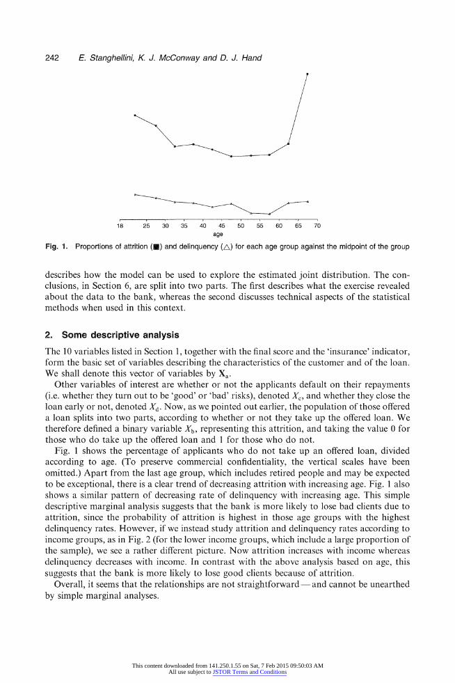
Fig. 1. Proportions of attrition (U) and delinquency (A) for each age group against the midpoint of the group

describes how the model can be used to explore the estimated joint distribution. The con- clusions, in Section 6, are split into two parts. The first describes what the exercise revealed about the data to the bank, whereas the second discusses technical aspects of the statistical methods when used in this context.

2. Some descriptive analysis

The 10 variables listed in Section 1, together with the final score and the 'insurance' indicator, form the basic set of variables describing the characteristics of the customer and of the loan. We shall denote this vector of variables by Xa.

Other variables of interest are whether or not the applicants default on their repayments (i.e. whether they turn out to be 'good' or 'bad' risks), denoted Xc, and whether they close the loan early or not, denoted Xd. Now, as we pointed out earlier, the population of those offered a loan splits into two parts, according to whether or not they take up the offered loan. We therefore defined a binary variable Xb, representing this attrition, and taking the value 0 for those who do take up the offered loan and 1 for those who do not.

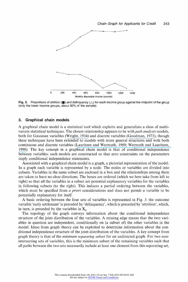
Fig. 1 shows the percentage of applicants who do not take up an offered loan, divided according to age. (To preserve commercial confidentiality, the vertical scales have been omitted.) Apart from the last age group, which includes retired people and may be expected to be exceptional, there is a clear trend of decreasing attrition with increasing age. Fig. I also shows a similar pattern of decreasing rate of delinquency with increasing age. This simple descriptive marginal analysis suggests that the bank is more likely to lose bad clients due to attrition, since the probability of attrition is highest in those age groups with the highest delinquency rates. However, if we instead study attrition and delinquency rates according to income groups, as in Fig. 2 (for the lower income groups, which include a large proportion of the sample), we see a rather different picture. Now attrition increases with income whereas delinquency decreases with income. In contrast with the above analysis based on age, this suggests that the bank is more likely to lose good clients because of attrition.

Overall, it seems that the relationships are not straightforward and cannot be unearthed by simple marginal analyses.

This content downloaded from 141.250.1.55 on Sat, 7 Feb 2015 09:50:03 AMAll use subject to JSTOR Terms and Conditions

Chain Graph for Applicants for Credit 243

0 200 400 600 800 1000 1200 1400

Monthly disposable income (pounds)

Fig. 2. Proportions of attrition (-) and delinquency (A) for each income group against the midpoint of the group (only the lower income groups, about 80% of the sample)

3. Graphical chain models

A graphical chain model is a statistical tool which exploits and generalizes a class of multi- variate statistical techniques. The closest relationship appears to be with path analysis models, both for Gaussian variables (Wright, 1934) and discrete variables (Goodman, 1973), though these techniques have been extended to models with more general structures and with both continuous and discrete variables (Lauritzen and Wermuth, 1989; Wermuth and Lauritzen, 1990). The key concept in a graphical chain model is that of conditional independence between variables: such models are constructed so that zero constraints on the parameters imply conditional independence statements.

Associated with a graphical chain model is a graph, a pictorial representation of the model. In a graph each variable is represented by a node. The nodes or variables are divided into subsets. Variables in the same subset are enclosed in a box and the relationships among them are taken to have no clear directions. The boxes are ordered (which we here take from left to right) so that all the variables in a subset are potential explanatory variables for the variables in following subsets (to the right). This induces a partial ordering between the variables, which must be specified from a priori considerations and does not permit a variable to be potentially explanatory for itself.

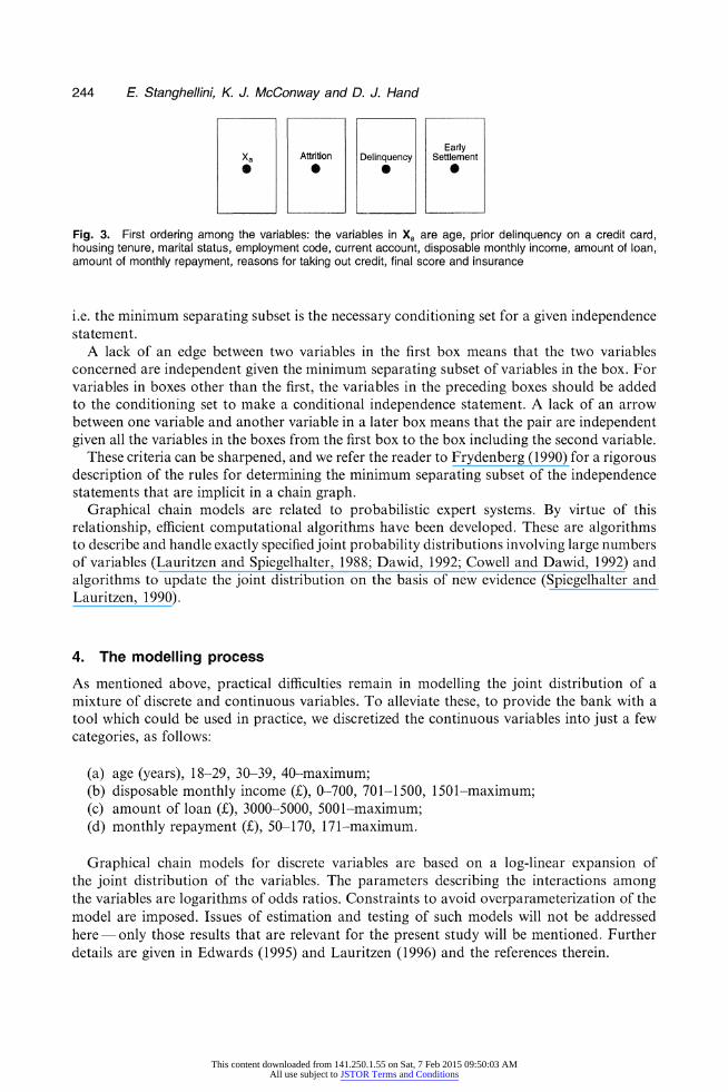
A basic ordering between the four sets of variables is represented in Fig. 3: the outcome variable 'early settlement' is preceded by 'delinquency', which is preceded by 'attrition', which, in turn, is preceded by the variables in Xa.

The topology of the graph conveys information about the conditional independence structure of the joint distribution of the variables. A missing edge means that the two vari- ables in question are independent, conditionally on (a subset of) the other variables in the model. Ideas from graph theory can be exploited to determine information about the con- ditional independence structure of the joint distribution of the variables. A key concept froin graph theory is that of the minimum separatinig subset for an undirected graph. For two non- intersecting sets of variables, this is the minimum subset of the remaining variables such that all paths between the two sets necessarily include at least one element from this separating set,

This content downloaded from 141.250.1.55 on Sat, 7 Feb 2015 09:50:03 AMAll use subject to JSTOR Terms and Conditions

244 E. Stanghellini, K. J. McConway and D. J. Hand

Early Xa Afttbon Delinquency Settlement 0 0 0

Fig. 3. First ordering among the variables: the variables in Xa are age, prior delinquency on a credit card, housing tenure, marital status, employment code, current account, disposable monthly income, amount of loan, amount of monthly repayment, reasons for taking out credit, final score and insurance

i.e. the minimum separating subset is the necessary conditioning set for a given independence statement.

A lack of an edge between two variables in the first box means that the two variables concerned are independent given the minimum separating subset of variables in the box. For variables in boxes other than the first, the variables in the preceding boxes should be added to the conditioning set to make a conditional independence statement. A lack of an arrow between one variable and another variable in a later box means that the pair are independent given all the variables in the boxes from the first box to the box including the second variable.

These criteria can be sharpened, and we refer the reader to Frydenberg (1990) for a rigorous description of the rules for determining the minimum separating subset of the independence statements that are implicit in a chain graph.

Graphical chain models are related to probabilistic expert systems. By virtue of this relationship, efficient computational algorithms have been developed. These are algorithms to describe and handle exactly specified joint probability distributions involving large numbers of variables (Lauritzen and Spiegelhalter, 1988; Dawid, 1992; Cowell and Dawid, 1992) and algorithms to update the joint distribution on the basis of new evidence (Spiegelhalter and Lauritzen, 1990).

4. The modelling process

As mentioned above, practical difficulties remain in modelling the joint distribution of a mixture of discrete and continuous variables. To alleviate these, to provide the bank with a tool which could be used in practice, we discretized the continuous variables into just a few categories, as follows:

(a) age (years), 18-29, 30-39, 40-maximum; (b) disposable monthly income (f), 0-700, 701-1500, 1501-maximum; (c) amount of loan (f), 3000-5000, 5001-maximum; (d) monthly repayment (?), 50-170, 171-maximum.

Graphical chain models for discrete variables are based on a log-linear expansion of the joint distribution of the variables. The parameters describing the interactions among the variables are logarithms of odds ratios. Constraints to avoid overparameterization of the model are imposed. Issues of estimation and testing of such models will not be addressed here only those results that are relevant for the present study will be mentioned. Further details are given in Edwards (1995) and Lauritzen (1996) and the references therein.

This content downloaded from 141.250.1.55 on Sat, 7 Feb 2015 09:50:03 AMAll use subject to JSTOR Terms and Conditions

Chain Graph for Applicants for Credit 245

4.1. Collapsibility and incomplete data Our aim is to model the joint distribution of the variables (Xa, Xb, Xc, Xd). We could, of course, restrict our investigation simply to those who take up the offer. This would allow us to make predictions about the likely behaviour, in terms of the outcome variables, Xc and Xd, of applicants with a given Xa-vector, as well as to characterize those Xa-values that are likely to lead to good outcomes. Such a restricted exercise would be of value to the bank. However, it would be even more valuable if we could build a model which would permit us to explore the effects of changes in banking policy e.g. how a change in the amount of the monthly repayment affects the rate of attrition and the rate of delinquency. It would also be attractive if we could see how the decision to sell or not to sell insurance affects both attrition and delinquency. As policy changes can, in general, affect attrition as well as the outcome vari- ables, we need to build a global model which includes all the four sets of variables.

The difficulty in modelling the joint distribution of these variables is that we observe Xc and Xd only for those applicants who take up the loan those who score 0 on Xb. This means, in particular, that the interactions between (Xc, Xd) and Xb cannot be observed. We can, however, make hypotheses about these interactions.

We assume that there are no arrows between Xb and Xc, Xd. This essentially says that, for people with a given vector Xa, whether they take up the loan or not has no relationship to whether or not they (would) default or repay. By noting that an implication is that

P(Xc, Xd IXa , Xb) = P(Xc, Xd IXa),

we observe that the above condition is sufficient to permit us to recover the joint distribution of the four variables from the observed data. Note that, without further assumptions, this condition does not imply that the conditional distribution (Xi,, Xc, Xd)lXb = 0 is equal to the conditional distribution (Xa, Xc, Xd)lXb = 1. (A suitable extra condition which would make these two conditional distributions identical is that X, is independent of Xb, Xa 11 Xb. How- ever, this is unlikely to hold in practice.) In the terminology of Rubin (1976), the condition Xb 11 (XC, Xd)IXa corresponds to data which are missing at random and this condition plus the extra condition Xa 11 Xb correspond to data which are mnissing completely at randomn.

Another way of looking at this is to observe that if Xb 11 (Xc, Xd)lXa then this condition ensures that the graph is collapsible on the (Xa, Xb) variables. There are various definitions of collapsibility for which we refer the reader to Whittaker (1990), chapter 12. Here we use the notion in the sense of Edwards (1995), pages 90-102. In words, an undirected graph is collapsible onto a subset of variables if and only if the boundary of every connected com- ponent of the variables not in the subset is complete. For a chain graph, collapsibility must be established on the skeleton of the graph, i.e. the graph without boxes obtained by dis- regarding the information about the type of the edge (see Cox and Wermuth (1996), p. 31, for the definition).

One implication of collapsibility is that the interaction parameters of the marginal distri- bution of (Xa, Xb) are equal to the corresponding parameters of the joint distribution of (X,, Xb, Xc, Xd). As the remaining parameters of the log-linear expansion of the joint distribution of (XMI, Xb, Xc, Xd) are equal to the corresponding parameters of the conditional distribution of (Xa, Xc, Xd)lXb = 0, which is the distribution that we observe, the parameters of the joint distribution can be derived from the corresponding terms of the above marginal and con- ditional distributions.

Collapsibility is a property of the topology of the graph and is therefore a property of the population. However, it also has strong implications for the estimation of a model.

This content downloaded from 141.250.1.55 on Sat, 7 Feb 2015 09:50:03 AMAll use subject to JSTOR Terms and Conditions

246 E. Stanghellini, K. J. McConway and D. J. Hand

(s) (t) Marital (w) Loan (i) Status Current A/C Amount Insurance

9 (f) 9(d) (e) II Final I(b) (c) Early Age Score Attrition Delinquency Settlement

Employm t using Tenure

C/Card Loan Monthly Income Delinquency Purpose Repayment

(r) Iy (u) (in) III II

Missing Arrows: None p>w s>t None e>i s>b p >c e>d

s>y s>u s>i h>b h >c s >d h>y h>u y>i y>b w >c h>d r >y w>u u>i t>b t >c i >d

y>u e>m f >b u >c b >d s>m m>b m>c c >d w>m b >c y > m u > m

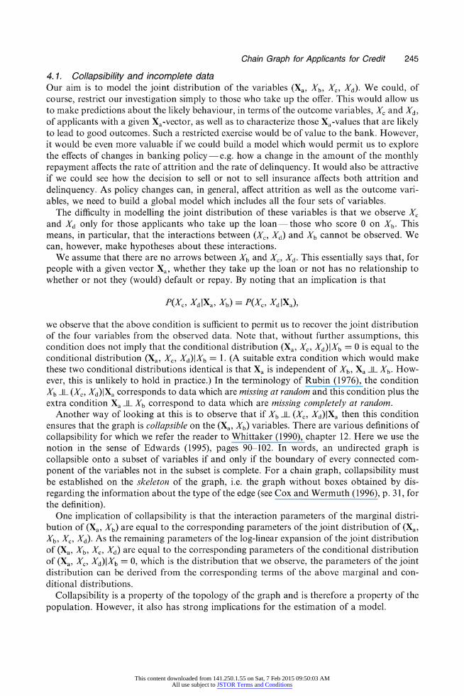
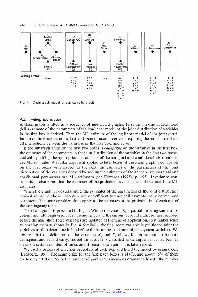
Fig. 4. Chain graph model for applicants for credit

4.2. Fitting the model A chain graph is fitted as a sequence of undirected graphs. First the maximum likelihood (ML) estimate of the parameters of the log-linear model of the joint distribution of variables in the first box is derived. Then the ML estimate of the log-linear model of the joint distri- bution of the variables in the first and second boxes is derived, requiring the model to include all interactions between the variables in the first box, and so on.

If the subgraph given by the first two boxes is collapsible on the variables in the first box, the estimates of the parameters in the joint distribution of the variables in the first two boxes, derived by adding the appropriate parameters of the marginal and conditional distributions, are ML estimates. A similar argument applies to later boxes: if the chain graph is collapsible on the first boxes with respect to the next, the estimates of the parameters of the joint distribution of the variables derived by adding the estimates of the appropriate marginal and conditional parameters are ML estimates (see Edwards (1995), p. 195). Invariance con- siderations also mean that the estimates of the probabilities of each cell of the model are ML estimates.

When the graph is not collapsible, the estimates of the parameters of the joint distribution derived using the above procedure are not efficient but are still asymptotically normal and consistent. The same considerations apply to the estimates of the probabilities of each cell of the contingency table.

The chain graph is presented in Fig. 4. Within the vector Xa a partial ordering can also be determined: although credit card delinquency and the current account indicator are recorded before the mail shot, these variables are updated at the time of application, so it makes sense to position them as shown in Fig. 4. Similarly, the final score variable is positioned after the variables used to determine it, but before the insurance and monthly repayment variables. We observe that the definition of the variables Xc and Xd allows for an account to be both delinquent and repaid early. Indeed an account is classified as delinquent if it has been in arrears a certain number of times and it remains so even if it is later repaid.

We used a backward selection procedure at each step and fitted the model by using CoCo (Badsberg, 1991). The sample size for the first seven boxes is 14473, and about 15% of them are lost by attrition. Since the number of parameters increases dramatically with the number

This content downloaded from 141.250.1.55 on Sat, 7 Feb 2015 09:50:03 AMAll use subject to JSTOR Terms and Conditions

Chain Graph for Applicants for Credit 247

of variables, a sparsity problem arises. We therefore decided to use the exact conditional likelihood ratio test (Kreiner, 1987), when the modelling process involved variables in boxes later than the third box. This forced us to restrict the model search in the last steps to the class of decomposable models (see Lauritzen (1996), chapter 4, for details). As the majority of the accounts are classified as good, there is a large proportion of empty cells in the contingency table when this variable is considered in the analysis. The significance level through all the analyses was set at 0.05.

In Fig. 4 the missing arrows between attrition and the other two outcome variables have a different meaning from the other missing arrows in the graph, since the associated hypotheses cannot be tested by using our data (see Section 3.1). We observe that the graph is collapsible on the first four boxes, so the estimate of the joint distribution is also an ML estimate. The collapsibility is lost in the fifth box because the final score is strongly related to all the variables in the preceding boxes and these do not form a complete subset. Therefore, the estimate of the joint distribution of the Xa-variables is not an ML estimate.

5. Exploring the estimated joint distribution

The bank would like to use the statistical model to investigate various aspects of the relationships between the variables, involving potentially complex manipulations of their estimated joint distribution. These manipulations require the calculation of marginal and conditional distributions of the log-linear model. We used the HUGIN software (Olesen et al., 1992) to manipulate the probabilities. Since the standard HUGIN interface handles only directed acyclic graphs, producing a 'compiled' undirected version, we translated the chain graph into an arbitrary directed acyclic graph with the same skeleton.

The estimation algorithms provide the exact marginal and conditional distributions of the variables provided that the joint distributions have been exactly specified. However, we are dealing with an estimated joint distribution. By an argument parallel to that in the previous section, any marginal distribution of a collapsible subset of variables obtained by mar- ginalizing an ML estimate of a joint distribution is an ML estimate. A similar argument applies to the conditional distribution if the conditioning subset is collapsible. Otherwise the estimated probabilities are consistent but not efficient estimates.

6. Conclusions

6. 1. The model The bank's first objective is to determine the population to target. Since the variables available before the mail shot are age and the credit card delinquency indicator, it is possible to inspect the behaviour of subgroups of the population produced by the cross-classification of these variables. This inspection led us to identify quite a large subgroup (we cannot state which for commercial reasons) which exhibited a delinquency probability about half the average and an attrition rate slightly less than average.

A second objective is to identify groups which are likely to demonstrate undesirable behaviour. We used the model to identify likely characteristics of customers who will turn out to be bad risks, who do not take out insurance on the loan and who do take up the loan (attrition, in this case, would be good for the bank).

A third objective concerns how changes in the bank's policy (e.g. the conditions associated with the offer of a loan) are likely to affect the behaviour of customers. A key role here is played by the insurance indicator: in a significant segment of the population, delinquency and

This content downloaded from 141.250.1.55 on Sat, 7 Feb 2015 09:50:03 AMAll use subject to JSTOR Terms and Conditions

248 E. Stanghellini, K. J. McConway and D. J. Hand

attrition are both lower for customers who do not take credit insurance than for those who do take insurance. There are several possible explanations:

(a) insurance increases the overall cost of the credit; price-sensitive custoiners may be less likely to take up a loan with an insurance premium;

(b) the protection given by insurance may make some customers less conscientious about their repayments;

(c) customers who believe themselves to be poor credit risks may also feel that they are more likely to fall ill or to lose their jobs; in other words, the option for insurance may communicate some information about the customer's perception of his or her own level of risk.

There is a trade-off for the lender in proposing insurance: for insured loans, the increase in attrition and delinquency reduces profits, but the insurance generates commission income and reduces the cost of delinquent accounts.

In another substantial subgroup, the risk of default is considerably worse for applicants who do not opt for insurance. This segment is partially defined by some prior delinquency on another credit product. As might be expected, the level of attrition is lower than average for this group, which has a demonstrated appetite for credit. In fact, it also suggests that the borrower who takes out insurance is cautious and that the prior delinquency is unlikely to be repeated on the new credit product.

This discussion suggests that the effect of insurance varies across segments of the portfolio. To maximize profitability, the lender may wish to offer insurance selectively to some segments of applicants and not to others.

As already mentioned, the monthly repayment variable is a deterministic function of the amount of the loan and of other variables not included in the study. To explore how changes in interest rate affect other variables, the term of credit should be included in the model to allow conditioning on its value. As it is, the model can be used to see the effects of changes in monthly repayment, keeping the interest rate constant. There is no direct edge between monthly repayment and attrition and no direct edge between monthly repayment and delin- quency the influence on these two variables is indirect and is via the insurance indicator. This may suggest that it is not the expected level of monthly repayments which affects these two variables, but further additional costs.

Monthly repayment is also related to early settlement. The marginal relationships suggest that early settlement is more likely for people with a low level of monthly repayment, but when we condition on small loan amounts we find that this relationship is reversed. We have found that such reversals between marginal and conditional relationships are quite common. Another example is the fact that, overall, married people are more likely to behave well in terms of delinquency but that this relationship is reversed for some subgroups. Such information is potentially important for the bank, and may lead to improved scoring systems.

We also note that the final score variable is not sufficient to separate the delinquency variables from the previous variables, and that some direct relationships remain (e.g. between income and delinquency). This means, essentially, that, for predicting delinquency, the final score does not capture all the information that is in its predictor variables: improved classi- fication rules could be built. Awareness of this can have important implications for the bank.

The work described in this paper was one of the first applications of graphical models in a credit scoring context, but our experience suggests that models of this kind hold great potential for such applications, offering insights into the data beyond those that are obtain- able by using standard credit scoring methods. To construct such models in house, a bank

This content downloaded from 141.250.1.55 on Sat, 7 Feb 2015 09:50:03 AMAll use subject to JSTOR Terms and Conditions

Chain Graph for Applicants for Credit 249

would require a small team comprising people who are familiar both with graphical models and with the data being modelled.

6.2. The method The general area of graphical and related models is currently attracting a tremendous amount of research attention, and rapid progress is being made (see, for example, Pearl (1995) and Buntine (1996) in addition to the references above). At the time of this project, however, there was no off-the-shelf software package which would permit integrated model selection, parameter estimation and probability propagation. We therefore had to use different pro- grams for each stage, as discussed above. Given the promising results of this project, and the relative ease with which similar projects will be able to be conducted in the future, it is clear that the general role for graphical models in consumer credit applications deserves further investigation.

An alternative elementary exploratory strategy to the construction of a graphical model is the careful use of multiple cross-tabulations. However, this has several shortcomings in the present application. In particular, of course, there is the danger of missing higher dimen- sional relationships which are lost by the marginalization process that is inherent in cross- tabulation. Graphical modelling helps us to decide which hypotheses to look at, as well as ultimately yielding an overall model.

The banking environment is increasingly dynamic and competitive. To react to this, banks need to assist their decision processes with flexible statistical tools which provide answers to various problems, many of them not specified at the time when the model was built. How- ever, accuracy is an important feature of any statistical model. There is a trade-off between these two issues. In Section 4.2 we noted that the estimate of the joint distribution in a chain graph model is not an ML estimate, unless some strong conditions on the topology of the graph are satisfied. Therefore, the estimates of the parameters are consistent but not efficient, and so are the estimates of the probabilities of the cells in the joint distribution.

To avoid the above loss of efficiency one possibility would be to derive an ML estimate of the undirected graph of the joint distribution. However, disregarding the ordering among the variables in the generating process may lead to graphs that are unacceptable, as an edge may be present in the undirected graph that does not correspond to an association between the variables in the generating process, or, conversely, parametric canicellation may obscure some associations. A discussion of these issues is contained in Cox and Wermuth (1996), chapter 8. Moreover, in our study, owing to the presence of the splitting variable attrition, fitting a joint graph for all the variables would be infeasible, and at least a two-step procedure would be necessary, leaving unsolved the problem of how to combine the estimates.

An alternative is to require that the graph is collapsible on each set of boxes, starting from the first, with respect to the next. However, this is a strong condition which is not necessarily satisfied. In our study, the presence of some variables strongly correlated with all the variables in the previous boxes, such as the final score, made this assumption unacceptable. Moreover, even when the graph satisfies this condition, any evaluation of a marignal of the joint dis- tributions which does not relate to a collapsible subset is not an efficient estimate of the marginal distribution, the efficiency being possible by obtaining separated ML estimates of different models. A parallel argument applies to the conditional distribution, if the con- ditioning subset is not collapsible.

The issue is, therefore, whether the loss of efficiency is compensated by a more realistic topology of the graph, in the first case, or a more flexible tool of analysis in the second. A

This content downloaded from 141.250.1.55 on Sat, 7 Feb 2015 09:50:03 AMAll use subject to JSTOR Terms and Conditions

250 E. Stanghellini, K J. McConway and D. J. Hand

common feature of banks' data sets is that they are reasonably large. As the consistency of the estimates is preserved, our view is that this provides a justification for the suggested use of graphical chain models in the credit scoring context.

A concern in any model fitting exercise, but perhaps especially relevant for a model as complex as that described in this paper, is the question of overfitting. Does our model go beyond fitting the underlying relationships between the variables to the extent of also fitting some of the random variation in the design sample? Overall, our model has 6746 parameters, approximately half in the first part of the model, based on about 14000 observations, and half in the second part, based on about 12000. However, the modular structure of the chain graph is such that the overfitting becomes dramatic in the last boxes. In classical multivariate analysis a rule of thumb of 5-10 times as many observations to variables is adopted. It is, in any case, merely a rule of thumb, and we do not yet have a feel for the applicability of this in models as complex as that outlined here. The topic of overfitting in complex models based on large data sets, as well as the development of suitable measures of goodness of fit, needs further work.

Acknowledgements

We would like to express our appreciation to the bank which funded this project for its vision and support throughout the work. We would also like to thank Gerard Scallan, for his helpful suggestions on an earlier draft of this paper, and a referee for painstaking and con- structive criticisms of an earlier draft. Some operational details of the application have been modified to maintain the confidentiality of the commercial context of the data. The revision of the paper has been made possible thanks to financial support from Consiglio Nazionale delle Ricerche, which is gratefully acknowledged.

References Badsberg, J. H. (1991) A guide to CoCo. Report. Institute for Electronic Systems, Aalborg. Buntine, W. (1996) A guide to the literature oni learning graphical models. IEEE Tranis. Know!l. Data Engng, 8,

195-210. Cowell, R. G. and Dawid, A. P. (1992) Fast retraction of evidence in a probabilistic expert systenm. Statist. Compilt.,

2, 37-40. Cox, D. R. and Wermuth, N. (1996) Multivariate Dependencies: Models, Analysis anid Interpretationi. London:

Chapman and Hall. Dawid, A. P. (1992) Applications of a general propagation algorithm for probabilistic expert system. Statist.

Comiipult., 2, 25-36. Edwards, D. (1995) Initrodulction to Gr-aphical Modelling. New York: Springer. Frydenberg, M. (1990) The chain graph Markov property. Scanid. J. Statist., 17, 333-353. Goodman, L. A. (1973) The analysis of multidimensional contingency tables when some variables are posterior to

others: a modified path analysis approach. Biomnetrika, 60, 179-192. Hand, D. J. and Henley, W. E. (1997) Statistical classification methods in consumer credit scoring: a review. J. R.

Statist. Soc. A, 160, 523-541. Hand, D. J. and Jacka, S. (eds) (1998) Statistics in Finiance. London: Arnold. Hand, D. J., McConway, K. J. and Stanghellini, E. (1996) Graphical models of applicants for credit. IMA J. Math.

Appl. Buls. Indstry, 8, 143-155. Kreiner, S. (1987) Analysis of multidimensionial contingency tables by exact conditionial tests: techniques and

strategies. Scand. J. Statist., 14, 97-112. Lauritzen, S. L. (1996) Graphical Models. Oxford: Oxford University Press. Lauritzen, S. L. and Spiegelhalter, D. J. (1988) Local computations with probabilities oni graphical structures and

their application to expert systems (with discussion). J. R. Statist. Soc. P, 50, 157-224. Lauritzen, S. L. and Wermuth, N. (1989) Graphical models for associations between variables, some of which are

qualitative and some quantitative. Ann. Math. Statist., 17, 31-54. Marshall, K. T. and Oliver, R. M. (1995) Decision Making and Forecasting. New York: McGraw-Hill.

This content downloaded from 141.250.1.55 on Sat, 7 Feb 2015 09:50:03 AMAll use subject to JSTOR Terms and Conditions

Chain Graph for Applicants for Credit 251

Olesen, K. G., Lauritzen, S. L. and Jensen, F. V. (1992) HUGIN: a system creating adaptive causal probabilistic networks. In Unicertainity in Artificial Intelligence (eds D. Dubois, M. P. Wellman, B. D'Ambrosio and P. Smets), vol. 8, pp. 223-229. San Mateo: Morgan Kaufmann.

Pearl, J. (1995) Causal diagrams for empirical research. Bionletrika, 82, 669-710. Rosenberg, E. and Gleit, A. (1994) Quantitative methods in credit management: a survey. Ops Res., 42, 589-613. Rubin, D. B. (1976) Inference and missing data (with discussion). Biomnetrika, 63, 581-592. Spiegelhalter, D. J. and Lauritzen, S. L. (1990) Sequential updating of conditional probabilities on directed graphical

structures. Networks, 20, 579-605. Thomas, L. C., Crook, J. N. and Edelman, D. B. (eds) (1992) Credit Scorinlg and Credit Control. Oxford: Clarendonl. Wermuth, N. and Lauritzen, S. L. (1990) On substantive research hypotheses, conditional independence graphs and

graphical chain models (with discussion). J. R. Statist. Soc. B, 52, 21-72. Whittaker, J. (1990) Graphical Models in Applied Mulltivariate Statistics. Chichester: Wiley. Wright, S. (1934) The method of path coefficients. Annti. Math. Statist., 5, 161-215.

This content downloaded from 141.250.1.55 on Sat, 7 Feb 2015 09:50:03 AMAll use subject to JSTOR Terms and Conditions