A Direct Georeferencing Imaging Technique to IdentifyEarth Surface Temperatures Using Oblique Angle

Airborne Measurements

byRyan Andrew Everett Byerlay

A Thesispresented to

The University of Guelph

In partial fulfilment of requirementsfor the degree of

Master of Applied Sciencein

Engineering

Guelph, Ontario, Canadac© Ryan A. E. Byerlay, December, 2019

ABSTRACT

A DIRECT GEOREFERENCING IMAGING TECHNIQUE TO IDENTIFY EARTH

SURFACE TEMPERATURES USING OBLIQUE ANGLE AIRBORNE

MEASUREMENTS

Ryan A. E. Byerlay Advisors:

University of Guelph, 2019 Dr. Amir A. Aliabadi

Dr. Mohammad Biglarbegian

This thesis describes a novel, open-source image processing method that directly georef-

erences oblique angle thermal images of the Earth’s surface and calculates Earth surface

temperatures at a high spatiotemporal resolution. Images were collected from a thermal

camera mounted on the Tethered And Navigated Air Blimp 2 (TANAB2). Median surface

temperatures are represented spatially in six four-hour time interval plots to display diurnal

surface temperature variation. The technique is applied to two data sets collected during

two separate field campaigns, one from a northern Canadian mining facility and one from

the University of Guelph, Guelph, Ontario, Canada. A comparison between surface tem-

peratures for images recorded from the mining facility and a MODerate resolution Imaging

Spectroradiometer (MODIS) image is completed with a resulting median absolute error of

0.64 K, bias of 0.5 K, and Root Mean Square Error (RMSE) of 5.45 K. Based on the find-

ings, the developed direct georeferencing oblique angle thermal image processing method is

capable of calculating surface temperatures with an accuracy of approximately 5 K at a spa-

tiotemporal resolution that is significantly higher than conventional satellite-based sensors.

Further applications of this direct georeferencing workflow are numerous and can be evalu-

ated with other cameras such as Red Green Blue (RGB), multispectral, and hyperspectral

imaging systems.

iii

Dedication

I would like to dedicate this work to my family, friends, teachers, and most of all my

parents for their encouragement and support throughout my educational pursuit.

iv

Acknowledgements

This work could not have been completed without the exceptional support and guidance

provided by my advisor Dr. Amir A. Aliabadi and my co-advisor Dr. Mohammad Biglarbe-

gian. Their thoughts and provision of new ideas were invaluable throughout the duration of

my graduate studies. I would also like to thank my colleagues Dr. Manoj K. Kizhakkeniyil,

Amir Nazem, Md. Rafsan Nahian, Dr. Mojtaba Ahmadi-Baloutaki, Seyedahmad Kia, and

Mohsen Moradi who assisted with the collection of data used in this work and provided

helpful support throughout the duration of my research.

Completing this work would not be possible without the technical support of Rowan

Williams Davies and Irwin Inc. (RWDI) and financial support from the University of Guelph,

the Ed McBean philanthropic fund, the Discovery Grant program (401231) from the Natural

Sciences and Engineering Research Council (NSERC) of Canada, the Government of Ontario

through the Ontario Centres of Excellence (OCE) under the Alberta-Ontario Innovation

Program (AOIP) (053450), and from Emission Reduction Alberta (ERA) (053498).

The Tethered And Navigated Air Blimp 2 (TANAB2) was partially developed by the assis-

tance of Denis Clement, Jason Dorssers, Katharine McNair, James Stock, Darian Vyriotes,

Amanda Pinto, and Phillip Labarge. The TANAB2 tether reel system was developed by An-

drew F. Byerlay. TANAB2 gondola electrical configuration advice provided by C. Harrison

Brodie is appreciated. Steve Nyman, Chris Duiker, Peter Purvis, Manuela Racki, Jeffrey

Defoe, Joanne Ryks, Ryan Smith, James Bracken, and Samantha French at the University

v

of Guelph assisted with field campaign logistics. Special credit is directed toward Amanda

Sawlor, Datev Dodkelian, Esra Mohamed, Di Cheng, Randy Regan, Margarent Love, and

Angela Vuk at the University of Guelph for administrative support. The computational

platforms were set up with the assistance of Jeff Madge, Joel Best, and Matthew Kent at

the University of Guelph. Technical discussions with John D. Wilson and Thomas Flesch

at the University of Alberta are highly appreciated. Field support from Alison M. Seguin

(RWDI), Andrew Bellavie (RWDI), and James Ravenhill at Southern Alberta Institute of

Technology (SAIT) is appreciated.

Most of all, I would like to express my sincere gratitude to my parents. Their endless

emotional and financial support towards my education contributed immeasurably to this

work.

vi

Table of Contents

Abstract ii

Dedication iv

Acknowledgements v

List of Tables ix

List of Figures xi

List of Abbreviations xii

List of Mathematical Symbols xiv

1 Introduction 11.1 Literature Review . . . . . . . . . . . . . . . . . . . . . . . . . . . . . . . . . 1

1.1.1 Measurement . . . . . . . . . . . . . . . . . . . . . . . . . . . . . . . 11.1.2 Direct Georeferencing . . . . . . . . . . . . . . . . . . . . . . . . . . . 51.1.3 Thermal and Oblique Imaging . . . . . . . . . . . . . . . . . . . . . . 5

1.2 Technology Gaps . . . . . . . . . . . . . . . . . . . . . . . . . . . . . . . . . 61.3 Objectives . . . . . . . . . . . . . . . . . . . . . . . . . . . . . . . . . . . . . 71.4 Thesis Structure . . . . . . . . . . . . . . . . . . . . . . . . . . . . . . . . . . 7

2 Method Development 82.1 Experimental Materials . . . . . . . . . . . . . . . . . . . . . . . . . . . . . . 82.2 Field Campaigns . . . . . . . . . . . . . . . . . . . . . . . . . . . . . . . . . 9

2.2.1 Mining Site Campaign . . . . . . . . . . . . . . . . . . . . . . . . . . 92.2.2 Guelph Campaign . . . . . . . . . . . . . . . . . . . . . . . . . . . . . 12

2.3 Image Processing Method Development . . . . . . . . . . . . . . . . . . . . . 132.3.1 Georeferencing . . . . . . . . . . . . . . . . . . . . . . . . . . . . . . 152.3.2 Thermal Camera Calibration . . . . . . . . . . . . . . . . . . . . . . 23

2.4 Principal Component Analysis (PCA) . . . . . . . . . . . . . . . . . . . . . . 27

vii

3 Results and Discussion 283.1 Mining Site Campaign . . . . . . . . . . . . . . . . . . . . . . . . . . . . . . 28

3.1.1 Diurnal Surface Temperature . . . . . . . . . . . . . . . . . . . . . . 293.1.2 Satellite Comparison . . . . . . . . . . . . . . . . . . . . . . . . . . . 323.1.3 Principal Component Analysis (PCA) . . . . . . . . . . . . . . . . . . 36

3.2 Guelph Campaign . . . . . . . . . . . . . . . . . . . . . . . . . . . . . . . . . 37

4 Conclusion and Future Work 424.1 Conclusion . . . . . . . . . . . . . . . . . . . . . . . . . . . . . . . . . . . . . 42

4.1.1 Georeferencing . . . . . . . . . . . . . . . . . . . . . . . . . . . . . . 424.1.2 Thermal Imaging . . . . . . . . . . . . . . . . . . . . . . . . . . . . . 43

4.2 Future Work . . . . . . . . . . . . . . . . . . . . . . . . . . . . . . . . . . . . 44

References 45

Appendices 55

A Source Code 56A.1 Thermal Camera Calibration . . . . . . . . . . . . . . . . . . . . . . . . . . . 56

A.1.1 Thermal Camera Calibration Plots . . . . . . . . . . . . . . . . . . . 58A.2 Mining Site Campaign . . . . . . . . . . . . . . . . . . . . . . . . . . . . . . 64

A.2.1 TriSonica Atmospheric Pressure to Altitude . . . . . . . . . . . . . . 64A.2.2 Spatial Coordinate Grid Overlaid on Mine Site . . . . . . . . . . . . . 75A.2.3 Emissivity Data Retrieval . . . . . . . . . . . . . . . . . . . . . . . . 79A.2.4 Direct Georeferencing and Temperature Calculation . . . . . . . . . . 82A.2.5 Data Separation for Diurnal Temperature Mapping . . . . . . . . . . 152A.2.6 Applying Thermal Camera Calibration Constants to Land Surface

Temperatures . . . . . . . . . . . . . . . . . . . . . . . . . . . . . . . 160A.2.7 Surface Temperature Map and Boxplots . . . . . . . . . . . . . . . . 183A.2.8 Principal Component Analysis (PCA) . . . . . . . . . . . . . . . . . . 221

A.3 Guelph Campaign . . . . . . . . . . . . . . . . . . . . . . . . . . . . . . . . . 229A.3.1 Identify TANAB2 Ascending and Descending Times . . . . . . . . . . 229A.3.2 TriSonica Atmospheric Pressure to Altitude . . . . . . . . . . . . . . 235A.3.3 Spatial Coordinate Grid Overlaid on University of Guelph Campus . 240A.3.4 Direct Georeferencing and Temperature Calculation . . . . . . . . . . 244A.3.5 Data Separation for Diurnal Temperature Mapping . . . . . . . . . . 305A.3.6 Surface Temperature Maps . . . . . . . . . . . . . . . . . . . . . . . . 313

B Published Work 347B.1 Peer-Reviewed Journal Papers . . . . . . . . . . . . . . . . . . . . . . . . . . 347B.2 Refereed Conferences . . . . . . . . . . . . . . . . . . . . . . . . . . . . . . . 347B.3 Poster Presentations . . . . . . . . . . . . . . . . . . . . . . . . . . . . . . . 348

viii

List of Tables

2.1 TANAB2 mining facility launch details. Times are in Local Daylight Time(LDT). . . . . . . . . . . . . . . . . . . . . . . . . . . . . . . . . . . . . . . . 12

2.2 TANAB2 launch details for July, 28, 2018 and August 13, 2018 Universityof Guelph, Guelph, Ontario, Canada deployments. Times are in EasternDaylight Time (EDT). . . . . . . . . . . . . . . . . . . . . . . . . . . . . . . 12

2.3 Default and calibrated camera parameters. . . . . . . . . . . . . . . . . . . . 262.4 Default and calibrated camera parameter statistics. . . . . . . . . . . . . . . 26

ix

List of Figures

2.1 (a) Diagram of the gondola on the TANAB2; (b) the TANAB2 deployed duringa field environmental monitoring campaign in May 2018. . . . . . . . . . . . 9

2.2 Diagram of the mining facility, where the black dots represent the edge ofthe facility, the red dots represent the outline of the open-pit mine, the tealdots represent the outline of the tailings pond, and the blue dots representwhere the TANAB2 was deployed during the field environmental monitoringcampaign in May 2018. . . . . . . . . . . . . . . . . . . . . . . . . . . . . . . 10

2.3 Use of three ropes controlled by personnel on the ground during a launch ofthe TANAB2 at the mining facility in May 2018. . . . . . . . . . . . . . . . . 11

2.4 Diagram of TANAB2 launches in relation to other notable buildings at ReekWalk, University of Guelph, Guelph, Ontario, Canada. . . . . . . . . . . . . 13

2.5 Process flow diagram of the image processing workflow. . . . . . . . . . . . . 142.6 Relationship between pixels and horizontal geographic distances. . . . . . . . 202.7 Relationship between vertical image pixels and the camera V FOV . . . . . . 212.8 Certified temperature compared to radiometric image pixel signal value for

water, soil, developed land, and grass. . . . . . . . . . . . . . . . . . . . . . . 25

3.1 Median temperatures over four-hour time intervals at 1 km × 1 km resolution;times are in Local Daylight Time (LDT). . . . . . . . . . . . . . . . . . . . . 30

3.2 Box plots representing temperature distribution over four-hour time intervalsfor the tailings pond and mine, where the orange line is the median tempera-ture; times are in Local Daylight Time (LDT). . . . . . . . . . . . . . . . . . 31

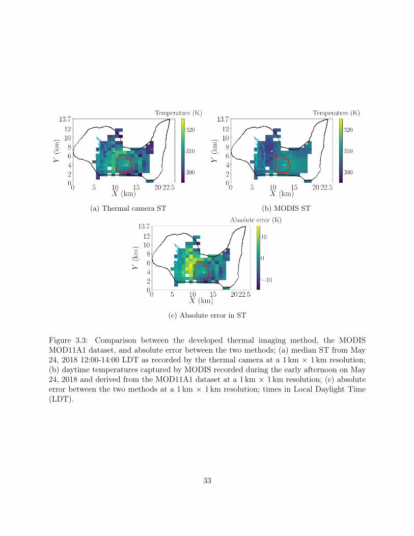
3.3 Comparison between the developed thermal imaging method, the MODISMOD11A1 dataset, and absolute error between the two methods; (a) medianST from May 24, 2018 12:00-14:00 LDT as recorded by the thermal cameraat a 1 km × 1 km resolution; (b) daytime temperatures captured by MODISrecorded during the early afternoon on May 24, 2018 and derived from theMOD11A1 dataset at a 1 km × 1 km resolution; (c) absolute error betweenthe two methods at a 1 km × 1 km resolution; times in Local Daylight Time(LDT). . . . . . . . . . . . . . . . . . . . . . . . . . . . . . . . . . . . . . . . 33

3.4 Representative horizontal directions encompassing the mining facility whichdisplay the largest surface temperature variation for each time interval; timesare in Local Daylight Time (LDT). . . . . . . . . . . . . . . . . . . . . . . . 36

x

3.5 Median surface temperatures over four-hour time intervals at 20 m × 20 mspatial resolution, where the red dot represents the TANAB2 launch location(Reek Walk), the black circle represents the Gryphon Centre Arena, the ma-genta circle represents the University Centre, the blue circle represents theAthletic Centre, the yellow circle represents Varsity Field, the cyan circle rep-resents Johnston Green, and the white circle represents the Fieldhouse. . . . 40

3.6 Median surface temperatures over four-hour time intervals at 50 m × 50 mspatial resolution, where the red dot represents the TANAB2 launch location(Reek Walk), the black circle represents the Gryphon Centre Arena, the ma-genta circle represents the University Centre, the blue circle represents theAthletic Centre, the yellow circle represents Varsity Field, the cyan circle rep-resents Johnston Green, and the white circle represents the Fieldhouse. . . . 41

xi

List of Abbreviations

ABI Advanced Baseline Imager

ALOS Advanced Land Observing Satellite

AVHRR Advanced Very High Resolution Radiometer

BBE BroadBand Emissivity

DEM Digital Elevation Model

DSM Digital Surface Model

EDT Eastern Daylight Time

ETM+ Enhanced Thematic Mapper Plus

GIS Geographic Information System

GNSS Global Navigation Satellite System

GOES Geostationary Operational Environmental Satellite

GPS Global Positioning System

HFOV Horizontal Field of View

HPR Horizontal Pixel Range

IMU Inertial Measurement Unit

LDT Local Daylight Time

LiDAR Light Detection And Ranging

LMFIT Non-Linear Least-Squares Minimization and Curve-Fitting

LWIR Long Wave Infrared Radiation

MODIS MODerate resolution Imaging Spectroradiometer

NASA National Aeronautics and Space Administration

NOAA National Oceanic and Atmospheric Administration

xii

PCA Principal Component Analysis

POES Polar-orbiting Operational Environmental Satellite

PPK Post-Processing Kinematic

PPP Precise Point Positioning

PRISM Panchromatic Remote-sensing for Stereo Mapping

RTK Real-Time Kinematic

RMSE Root Mean Square Error

ST Surface or Skin Temperature

sUAS small Unmanned Aerial System

TANAB2 Tethered And Navigated Air Blimp 2

TIR Thermal InfRared

TIRS Thermal InfRared Sensor

UAV Unmanned Aerial Vehicle

USGS United States Geological Survey

VFOV Vertical Field of View

VPR Vertical Pixel Range

xiii

List of Mathematical Symbols

Latin Symbolsa Constant

B Constant

BBE Emissivity

b Constant

c Constant

dedge Distance

dhoriz Distance

dhoriztop Distance

dlaunch Distance

F Constant

HFOV Angle

HPR Pixel

i Pixel

k Distance

Lat1 Latitude

Lat2 Latitude

lat1 Latitude

lat2 Latitude

Lon1 Longitude

Lon2 Longitude

lon1 Longitude

xiv

lon2 Longitude

n Integer

O Constant

P0 Pixel

P256 Pixel

P512 Pixel

P1 Pressure

P2 Pressure

Px Pixel

R1 Constant

R2 Constant

R Constant

z1 Altitude

z2 Altitude

zAGL Altitude

Slope Slope

TObj Temperature

Tv Temperature

UAtm Signal Value

UObj Signal Value

URefl Signal Value

UTot Signal Value

V FOV Angle

V PR Pixel

X Pixel

Y aw Angle

Y b Pixel

Y c Pixel

ypixel Pixel

xv

Y t Pixel

Y tx Pixel

Greek Symbolsα Angle

β Angle

η Angle

γ Angle

κ Angle

θ Angle

∆ Implies difference

ε Emissivity

ε29 Emissivity

ε31 Emissivity

ε32 Emissivity

τ Transmissivity

xvi

Chapter 1

Introduction

Earth surface temperature, otherwise known as Skin Temperature (ST), is an importantgeophysical variable that has been measured with remote sensing technologies since the1970s [60, 72]. Accurate quantification of ST is important for many Earth system models,including meteorological, climate, and planetary boundary layer models [58, 77, 89]. Micro-,meso-, and macro-scale climate models all consider ST as a key variable, as noted by Gémeset al. [28]. Land surface temperature is a key variable when quantifying the impacts ofurban heat islands. Specifically, the diurnal impact of ST with respect to the surroundingenvironment are of importance to many researchers [44, 59]. Furthermore, macro- and meso-scale models, including those that model the change of climate, consider ST over both landand waterbodies as a boundary condition [25, 34]. The impact of ST on large freshwaterlakes has also been studied as surface water temperature influences thermal stratification inlakes [49, 64].

1.1 Literature Review

1.1.1 Measurement

ST can be quantified as a function of Long Wave Infrared Radiation (LWIR) emitted fromthe Earth’s surface [100]. The emitted LWIR is an important variable when considering theEarth energy budget from incoming solar radiation [100]. Before the advent of satellites andother remote sensing platforms, multiple point sources recording either surface temperatureor air temperature were used in conjunction with weighting algorithms and other GeographicInformation Systems (GIS) techniques to spatially represent ST [75]. These historical meth-

1

ods can introduce significant inaccuracies during interpolation of the data, as a result, remotesensing tools have since been utilised to reduce these data analysis errors [75].

Satellite-Based Sensors

Conventionally, ST has been quantified from remote sensing satellites with onboard ST sen-sors including the MODerate resolution Imaging Spectroradiometer (MODIS), the AdvancedSpaceborne Thermal Emission and Reflection Radiometer (ASTER), the Advanced BaselineImager (ABI), the Enhanced Thematic Mapper Plus (ETM+), the Thermal InfRared Sensor(TIRS), and the Advanced Very High Resolution Radiometer (AVHRR) amongst other datasources [36, 89]. These sensors record data within the Thermal InfRared (TIR) or LWIRspectra between 8 and 15 µm [94].

MODIS is located on both the Terra and Aqua satellites which are operated by the Na-tional Aeronautics and Space Administration (NASA) [51]. Both satellites have polar, sun-synchronous orbits1,2 and both MODIS sensors record two distinct images daily at differenttimes, approximately three hours apart [19]. The horizontal resolution of MODIS images isapproximately 1 km × 1 km [56]. MODIS records data from 36 spectral bands in total whichinclude wavelengths between 0.41 and 14.4 µm, of specific importance for ST are the bands20 to 36 which cover the spectral range between 3.66 and 14.4 µm [56, 104]. In additionto MODIS, ASTER is also located onboard the Terra satellite [66]. ASTER images theEarth’s surface with a high spatial resolution of 90 m × 90 m and a revisit time of 16 daysfor each imaged location [30, 32]. ASTER contains three subsystems, including a systemwhich records data within the TIR spectrum between 8.13 and 11.7 µm.3

Geostationary Operational Environmental Satellite (GOES) satellites are operated througha collaboration between NASA and the National Oceanic and Atmospheric Administration(NOAA).4 The GOES-R series of satellites are the most recent geostationary satellites to bedeveloped and launched by this partnership, specifically GOES-16 and GOES-17 which wereoperational as of December 18, 2017 and February 12, 2019 respectively5,6 [4]. Onboardboth GOES-16 and GOES-17, the ABI records images for 16 spectral bands which rangebetween 0.45 and 13.6 µm7 [83]. The ABI on GOES-R series satellites records images over

1https://aqua.nasa.gov/content/about-aqua2https://terra.nasa.gov/about3https://asterweb.jpl.nasa.gov/characteristics.asp4https://www.nasa.gov/content/goes-overview/index.html5https://www.goes-r.gov/users/transitionToOperations16.html6https://www.goes-r.gov/users/transitionToOperations17.html7https://www.goes-r.gov/spacesegment/ABI-tech-summary.html

2

the continental United States every 5 minutes for all 16 spectral bands and at a spatialresolution of 2 km × 2 km [17, 82].

Landsat satellites are developed and operated by NASA in collaboration with the UnitedStates Geological Survey (USGS).8 Currently, Landsat 7 ETM+ records images with eightspectral bands, one of which records within the 10.4 and 12.5 µm spectrum. Landsat 8 TIRSrecords images with 11 spectral bands; one band records data within the 10.6 to 11.19 µm

range and another records data within the 11.5 to 12.5 µm range [23]. Landsat 7 ETM+records TIR data at a spatial resolution of 60 m × 60 m, while Landsat 8 TIRS records TIRdata at a spatial resolution of 120 m × 120 m [37]. Both Landsat 7 and 8 have a revisit timeperiod of 16 days [15].

AVHRR is a sensor that is operated by NOAA and is located onboard the Polar orbitingOperational Environmental Satellites (POES) series [41]. The third generation AVHRR islocated onboard NOAA-15, -16, -17, -18, and -19, of which NOAA-15, -18, and -19 are stilloperational [41].9 AVHRR has 6 channels in total and two channels which image withinthe LWIR spectrum, one channel records data within the 10.3 to 11.3 µm range while theother channel records data within the 11.5 to 12.5 µm range.10 The NOAA-15, -18, and-19 satellites are sun-synchronous polar orbiting satellites and AVHRR records images at aspatial resolution of 1.1 km × 1.1 km. These satellites have a short revisit period that variesbetween four and six AVHRR revisits per day as AVHRR is located on multiple satellites[43, 47, 52].

Although there are many remote sensing instruments which map ST, satellite-based STsources have limitations, for example, land surface temperature measurements are impactedby the atmosphere and surface emissivity [54]. If atmospheric characteristics are known, analgorithmic model can be used to extract land surface temperature from satellite imagery[62]. Even with corrections to quantify ST, both high spatial and temporal resolution landsurface temperature data is not available from satellite sources [11]. High spatial resolutiondata is associated with low temporal resolution data and high temporal resolution data isassociated with low spatial resolution data [11, 106]. Furthermore, satellites are known tobe impacted by cloud cover, atmospheric dust, and sensor failure [57, 68]. Miniaturisationof thermal imaging technologies and the development of reliable Unmanned Aerial Vehicles(UAVs) and Unmanned Aerial Systems (UASs), such as drones, kites, and blimps, provide

8https://landsat.gsfc.nasa.gov/9https://www.ospo.noaa.gov/Operations/POES/status.html

10https://noaasis.noaa.gov/NOAASIS/ml/avhrr.html

3

another airborne platform to derive ST from images [7, 48]. Furthermore, coupling smallUnmanned Aerial System (sUAS) platforms with oblique thermal imaging technology andconcurrent image processing methods can result in increased ST coverage.

Unmanned Aerial Systems

Recently it has become increasingly common for sUAS platforms to include thermal cameras[18]. Uncooled thermal cameras are most often used on sUASs as they are physically lighter,inexpensive, and require less power to operate as compared to cooled thermal cameras [74,80, 84]. There are many types of sUAS devices used to deploy camera systems, includingbut not limited to fixed wing and multi-rotor drones, kites, blimps, and balloons [21].

Tethered balloons are another aerial platform that have several advantages as comparedto conventional sUASs. Tethered balloons can be deployed for hours without changingbatteries, be launched in remote and complex environments where drones are unable to fly(e.g. airports), are inexpensive relative to other sUAS platforms, and their altitude can beprecisely controlled, amongst other advantages [65, 96]. A few studies have been completedinvolving thermal imaging and tethered balloons. Vierling et al. [96] deployed a helium-filled, tethered aerostat equipped with a thermal infrared sensor, capable of lifting a payloadof 78 kg and flying in a maximum wind speed greater than 11 m s-1. Rahaghi et al. [74]launched a tethered-helium-filled balloon equipped with a FLIR Tau 2 thermal camera overLake Geneva, Switzerland, “under weak wind conditions.”

Airborne sUAS vectors, including drones and balloons, have been noted to be deployed inmaximum wind speeds up to 10 m s-1, after which sUAS performance is significantly degraded[78]. von Burern et al. [97] and Hardin et al. [31] reported that many manufacturers claimthat UAVs are capable of flying in wind speeds up to 8.3 m s-1. However, Hardin et al.[31] stated that wind speeds greater than 7 m s-1 can impact flight time and performance.Ren et al. [79] noted that the DJI Phantom 4 quadcopter, a popular drone produced forthe consumer market, has a maximum wind resistance speed of 10 m s-1. Puliti et al. [73]collected earth surface images from a UAV over multiple flights in wind speeds up to 7 m s-1,where each flight lasted approximately 24 minutes. Boon et al. [9] used two types of UAVs(fixed wing and multi-rotor) for an environmental mapping study. Both UAVs were capableof flying in a maximum wind speed of 11.1 m s-1. Rankin and Wolff [76] used a tetheredballoon during a field campaign in which the manufacturer recommended use in maximumwind speeds up to 12 m s-1, however the blimp was not flown in wind speeds above 8 m s-1.Hot-air-based balloons experience inflation and positioning difficultly in wind speeds greater

4

than 4.17 m s-1 and helium-filled balloons were found to be destabilised in winds greaterthan 1.4 m s-1 as described by Aber [1].

1.1.2 Direct Georeferencing

With advancing sUAS technology, including the integration of Inertial Measurement Units(IMUs) and Global Navigation Satellite System (GNSS) units, sUAS imaging systems havebeen able to directly georeference images without the use of ground control [18, 70, 86].The angular and positioning data provided by these systems can either be used directlyor processed with Real-Time Kinematic (RTK), Post-Processing Kinematic (PPK), PrecisePoint Positioning (PPP), or differential correction techniques prior to being utilised in di-rect georeferencing methods [6, 61, 86, 109]. Without the use of differential correction forgeographical coordinates calculated from direct georeferencing, positional accuracy in therange of 2 m to 5 m is typical [92, 102]. Padró et al. [70] quantified Root Mean Square Error(RMSE) for GNSS direct georeferencing without correction and PPK methods with respectto pre-defined ground control point locations. Planimetric RMSE for the uncorrected GNSSdirectly georeferenced data was 1.06 m, while vertical error was 4.21 m. The RMSE for thePPK methods were at least one order of magnitude less than that of the uncorrected directgeoreferencing method. However, Padró et al. [70] noted that the uncorrected GNSS ap-proach may be appropriate, such as in cases of analysing satellite images with a pixel sizegreater than 2 m.

1.1.3 Thermal and Oblique Imaging

Thermal cameras use microbolometer focal plane arrays to observe incoming radiant energy[26, 69]. When an image is captured, the microbolometer array represents the observedenergy as a signal value (commonly referred to as digital numbers or A/D counts) whichincludes the radiant energy emitted from the atmosphere, reflected by the surface, andrecorded from the imaged surface of the object [107]. Microbolometer temperature is knownto vary as a function of sensor, camera, and ambient temperatures [12, 26, 55]. Cooledthermal cameras are significantly more sensitive than uncooled systems and provide moreaccurate, absolute temperatures [80]. However, current cooled camera technology requiresan airborne vector capable of lifting more than 4 kg, which is greater than the capacity ofsUAS and smaller tethered-balloon-system payloads [91]. It has been noted in literaturethat uncooled thermal cameras can be radiometrically calibrated to reduce uncooled camera

5

error to ±5 K [27, 46].Oblique imaging systems coupled with sUAS or tethered-balloon systems can significantly

increase the recorded land surface area as compared to nadir imaging systems. However,radiometric thermal imaging systems can be impacted from non-nadir setups, where surfacetemperature error is introduced as a function of observation angle [22]. Viewing anglesgreater than 30◦ of nadir over waterbodies have been noted to introduce surface temperatureerror of approximately 0.5 K [22, 45, 90]. This error is introduced as the surface emissivityof water changes as the viewing angle of the thermal camera becomes more oblique andreflected radiation from the surface increasingly influences the internal sensor of the thermalcamera [22]. Horton et al. [35] noted that sea surface temperature emissivity varied between0.36 and 0.98 for viewing angles between 90◦ (nadir) and 5◦ (below horizontal), respectively.James et al. [40] recorded ground-based oblique thermal images of lava flows and quantifieda ±3 % difference in radiative power from the lava flows where error increases as more distantobjects had high emissivities as compared to closer ones. More distant objects were likely tobe influenced the most by increasingly oblique viewing angles. In the study, they accountedfor atmospheric transmission effects of the radiation [40]. Hopkinson et al. [33] recordedground-based oblique thermal images of a glacier at varying diurnal times. It was noted thatthe maximum temperature difference was ±3 K, where the emissivity was assumed to be0.98 However, the calculated glacier surface temperatures were not validated. As a result, itis possible that these temperature variations could be influenced by transmitted and reflectedradiation.

1.2 Technology Gaps

High spatial and temporal resolution data of the Earth’s surface capable of characterisingdiurnal ST patterns is difficult to obtain from conventional remote sensing sources [58].Furthermore, the use of open-source direct georeferencing methods and surface temperaturecalculation for thermal images collected from airborne vectors at oblique angles are not widelyreported [95]. The coupling of direct georeferencing thermal images captured from a tethered-balloon-based vector is novel, and the focus of this thesis is the development of an open-source image processing workflow to map surface temperatures with a high spatiotemporalresolution.

6

1.3 Objectives

In this thesis, the development of an open-source, Python-based thermal image direct geo-referencing and ST calculation method is described and evaluated with respect to MODISsatellite imagery. The developed program quantifies ST at a high spatiotemporal resolutionas compared to conventional satellite sources. The images were collected during two differentfield campaigns, both of which will be detailed further, the first within a remote northernCanadian mining facility in May 2018 and the second on campus at the University of Guelphduring July and August 2018. The diurnal ST variation will be represented for both fieldcampaigns and trends will be discussed and explained.

1.4 Thesis Structure

The structure of this thesis is as follows:Chapter 1: An overview of current thermal remote sensing techniques is provided in

addition to recent advancements made in UAS remote sensing technology, direct georefer-encing, thermal imaging, and oblique imaging. Relevant literature supporting each topic isincluded and reviewed appropriately. This chapter also highlights the existing technologygaps in the presented research and details the objectives and motivation for this thesis.

Chapter 2: The specifics of the two field campaigns and instrumentation used to collectdata are detailed. Section 2.3.1 specifies the direct georeferencing method, Section 2.3.2specifies the ST calculation, and Section 2.3.2 specifies the calibration procedure applied tothe thermal camera used in both field experiments. Section 2.4 briefly describes the workflowused to develop the Principal Component Analysis (PCA).

Chapter 3: The results from the method discussed in Chapter 2, are displayed. DiurnalST variation, ST comparison to MODIS, and PCA figures are presented and discussed indetail with references to recently published, relevant literature.

Chapter: 4: Conclusions from Chapter 3 are reiterated and potential applications ofthe imaging workflow are discussed.

7

Chapter 2

Method Development

2.1 Experimental Materials

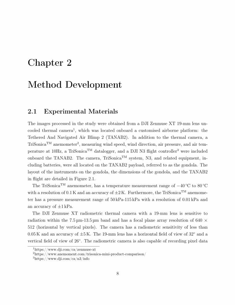
The images processed in the study were obtained from a DJI Zenmuse XT 19-mm lens un-cooled thermal camera1, which was located onboard a customised airborne platform: theTethered And Navigated Air Blimp 2 (TANAB2). In addition to the thermal camera, aTriSonicaTM anemometer2, measuring wind speed, wind direction, air pressure, and air tem-perature at 10Hz, a TriSonicaTM datalogger, and a DJI N3 flight controller3 were includedonboard the TANAB2. The camera, TriSonicaTM system, N3, and related equipment, in-cluding batteries, were all located on the TANAB2 payload, referred to as the gondola. Thelayout of the instruments on the gondola, the dimensions of the gondola, and the TANAB2in flight are detailed in Figure 2.1.

The TriSonicaTM anemometer, has a temperature measurement range of −40 ◦C to 80 ◦C

with a resolution of 0.1 K and an accuracy of ±2 K. Furthermore, the TriSonicaTM anemome-ter has a pressure measurement range of 50 kPa-115 kPa with a resolution of 0.01 kPa andan accuracy of ±1 kPa.

The DJI Zenmuse XT radiometric thermal camera with a 19-mm lens is sensitive toradiation within the 7.5 µm-13.5 µm band and has a focal plane array resolution of 640 ×512 (horizontal by vertical pixels). The camera has a radiometric sensitivity of less than0.05 K and an accuracy of ±5 K. The 19-mm lens has a horizontal field of view of 32◦ and avertical field of view of 26◦. The radiometric camera is also capable of recording pixel data

1https://www.dji.com/ca/zenmuse-xt2https://www.anemoment.com/trisonica-mini-product-comparison/3https://www.dji.com/ca/n3/info

8

(a) (b)

Figure 2.1: (a) Diagram of the gondola on the TANAB2; (b) the TANAB2 deployed duringa field environmental monitoring campaign in May 2018.

at 14-bit resolution.

2.2 Field Campaigns

2.2.1 Mining Site Campaign

During May 2018, the TANAB2 was deployed in a northern Canadian remote open-pit miningfacility. The specifics of the project, including the name of the mine, location, and client,cannot be disclosed due to the signing of a non-disclosure agreement with the industrialpartner of the project. As a result, figures included in this thesis are void of geographicalidentifying features, such as latitude and longitude data. Instead, ST in relation to the siteperimeter, tailings pond, and open-pit mine is quantified.

The TANAB2 and DJI thermal camera have been deployed and surface images have beenrecorded in a remote mining site in northern Canada during dawn, day, dusk, and night.The TANAB2 was deployed a total of twelve times at three different locations as denotedby Figure 2.2 [65]. Within the boundaries of the remote mining site, the TANAB2 andDJI camera setup were used in conjunction with a Lightbridge2 controller and either anAndroid- or iOS-powered smartphone. With the TANAB2 deployed, using the Lightbridge2,the thermal camera was tilted parallel to the horizon and was positioned at either the left

9

or right most Yaw maximum of the camera gimbal. Methodically, the camera was pannedhorizontally and an image was captured approximately every 5◦. When the maximum Yawlimitation of the gimbal was reached, the camera was tilted approximately 5◦ towards theEarth’s surface and the imaging procedure repeated again until the camera was perpendicularto the ground. This imaging procedure occurred approximately every hour during eachTANAB2 profile in an effort to record the diurnal variation of surface temperature.

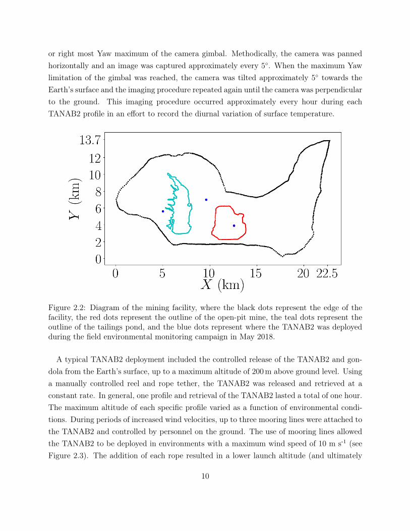
Figure 2.2: Diagram of the mining facility, where the black dots represent the edge of thefacility, the red dots represent the outline of the open-pit mine, the teal dots represent theoutline of the tailings pond, and the blue dots represent where the TANAB2 was deployedduring the field environmental monitoring campaign in May 2018.

A typical TANAB2 deployment included the controlled release of the TANAB2 and gon-dola from the Earth’s surface, up to a maximum altitude of 200 m above ground level. Usinga manually controlled reel and rope tether, the TANAB2 was released and retrieved at aconstant rate. In general, one profile and retrieval of the TANAB2 lasted a total of one hour.The maximum altitude of each specific profile varied as a function of environmental condi-tions. During periods of increased wind velocities, up to three mooring lines were attached tothe TANAB2 and controlled by personnel on the ground. The use of mooring lines allowedthe TANAB2 to be deployed in environments with a maximum wind speed of 10 m s-1 (seeFigure 2.3). The addition of each rope resulted in a lower launch altitude (and ultimately

10

less mapped area) due to addition of weight during periods of atmospheric instability suchas the afternoons. This trade-off was deemed acceptable as it was imperative to launch theTANAB2 in both stable and unstable atmospheric conditions to successfully map diurnalsurface temperatures. The TANAB2 was launched a total of 12 times at the mining facility(Figure 2.2), recording approximately 50 hours of TriSonicaTM data. The details of eachdeployment is noted in Table 2.1 below.

The DJI Zenmuse XT was also deployed either on top of stacked crates or on top of a ladderdeployed behind a stationary vehicle. In both instances, the camera had an altitude aboveground of approximately 2 m. The details of each surface-based thermal camera deploymentare included in Table 2.1 where the number of TANAB2 profiles is not specified.

Figure 2.3: Use of three ropes controlled by personnel on the ground during a launch of theTANAB2 at the mining facility in May 2018.

11

Table 2.1: TANAB2 mining facility launch details. Times are in Local Daylight Time (LDT).

Experiment Location Start date Start time End time No. Profiles Duration1 Tailings pond 2018/05/05 13:07:00 17:00:00 - 04:07:002 Tailings pond 2018/05/06 09:55:00 16:45:00 - 06:50:003 Tailings pond 2018/05/07 21:41:00 02:47:00 14 05:06:004 Tailings pond 2018/05/09 03:30:00 04:00:00 02 00:30:005 Tailings pond 2018/05/10 02:30:00 08:30:00 21 06:00:006 Tailings pond 2018/05/11 18:28:00 23:00:00 - 04:32:007 Tailings pond 2018/05/12 12:02:00 12:44:00 - 00:42:008 Tailings pond 2018/05/13 04:12:00 09:13:00 - 05:01:009 Tailings pond 2018/05/15 04:55:00 11:00:00 22 06:05:0010 Tailings pond 2018/05/17 05:37:00 09:00:00 - 03:23:0011 Mine 2018/05/18 04:12:00 11:12:00 20 07:00:0012 Mine 2018/05/19 18:52:00 23:15:00 17 04:23:0013 Mine 2018/05/21 11:00:00 12:17:00 04 01:17:0014 Mine 2018/05/23 01:47:00 05:30:00 10 02:43:0015 Mine 2018/05/24: 11:19:00 14:25:00 12 03:06:0016 Mine 2018/05/27 14:38:00 17:50:00 18 03:12:0017 Tailings pond 2018/05/30 10:55:00 18:57:00 24 08:02:0018 Tailings pond 2018/05/31 11:07:00 14:43:00 08 03:36:00

2.2.2 Guelph Campaign

The TANAB2 was launched at the University of Guelph, Guelph, Ontario, Canada on July28, 2018 and August 13, 2018. The launches occurred in the Reek Walk, a conventionaltwo-dimensional urban canyon, at 43.5323◦ N and 80.2253◦ W [63]. Specific launch sitegeographical features are illustrated in Figure 2.4, where the yellow dot represents the ReekWalk TANAB2 launch site and other proximal buildings are labelled appropriately. Thermalimages were captured between 05:04 and 21:21 Eastern Daylight Time (EDT) on July 28th

and between 05:20 and 20:31 EDT on August 13th. This field campaign seeked to identifythe diurnal ST variation of the campus buildings with respect to adjacent green spaces at ahigh spatiotemporal resolution. Images were captured in the same manner as described inSection 2.2.1. The details of the two TANAB2 deployments are described in Table 2.2.

Table 2.2: TANAB2 launch details for July, 28, 2018 and August 13, 2018 University ofGuelph, Guelph, Ontario, Canada deployments. Times are in Eastern Daylight Time (EDT).

Exp. Location Start date Start time End time No.Profiles Experiment time1 Reek Walk 2018/07/28 02:04:00 21:31:00 20 19:27:002 Reek Walk 2018/08/13 04:49:00 20:36:00 12 15:47:00

12

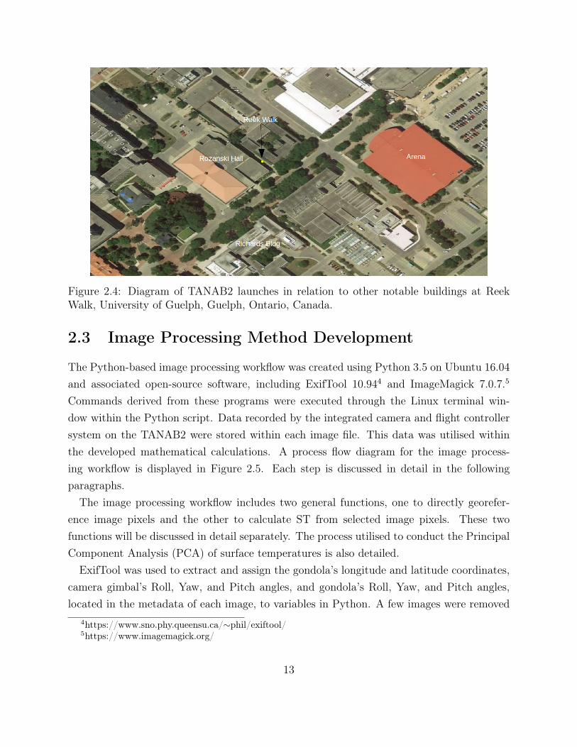
Figure 2.4: Diagram of TANAB2 launches in relation to other notable buildings at ReekWalk, University of Guelph, Guelph, Ontario, Canada.

2.3 Image Processing Method Development

The Python-based image processing workflow was created using Python 3.5 on Ubuntu 16.04and associated open-source software, including ExifTool 10.944 and ImageMagick 7.0.7.5

Commands derived from these programs were executed through the Linux terminal win-dow within the Python script. Data recorded by the integrated camera and flight controllersystem on the TANAB2 were stored within each image file. This data was utilised withinthe developed mathematical calculations. A process flow diagram for the image process-ing workflow is displayed in Figure 2.5. Each step is discussed in detail in the followingparagraphs.

The image processing workflow includes two general functions, one to directly georefer-ence image pixels and the other to calculate ST from selected image pixels. These twofunctions will be discussed in detail separately. The process utilised to conduct the PrincipalComponent Analysis (PCA) of surface temperatures is also detailed.

ExifTool was used to extract and assign the gondola’s longitude and latitude coordinates,camera gimbal’s Roll, Yaw, and Pitch angles, and gondola’s Roll, Yaw, and Pitch angles,located in the metadata of each image, to variables in Python. A few images were removed

4https://www.sno.phy.queensu.ca/∼phil/exiftool/5https://www.imagemagick.org/

13

Figure 2.5: Process flow diagram of the image processing workflow.

14

from the workflow due to excessive angles of the gondola or camera. The camera Roll angledid not significantly impact the method as the Zenmuse XT was self stabilised. However,if the gondola Roll degree was greater than 45◦ or less than −45◦, the camera becamedestabilised. Images with gondola Roll angles outside of this range were omitted from theworkflow. Furthermore, the mechanical Pitch range of the camera was noted to be between45◦ and −135◦. Gimbal Pitch angles greater than 0◦ primarily included images of the sky,gimbal Pitch angles equivalent to 0◦ were images of the horizon and gimbal Pitch anglesless than 0◦ included images primarily of the ground. It was determined that the recordedcamera gimbal Pitch angle corresponded to the Pitch angle for the middle of each image.Any images with a gimbal Pitch angle greater than or equal to −2◦ were omitted from theimage processing analysis. Furthermore, very oblique pitch angles, greater than −30◦ fromthe horizon, were noted to possibly introduce errors into the ST calculations6 but were notnecessarily eliminated. Based on physical parameters of the camera, including the Verticaland Horizontal Fields Of View (V FOV and HFOV ) angles, images with a gimbal Pitchangle less than or equivalent to −76◦ were also removed from the analysis. This filter waschosen because the bottom of the image would have a corresponding Pitch angle of therecorded gimbal Pitch angle, plus one half of the V FOV that would result in an angle closeto or less than −89◦ which may disrupt direct georeferencing calculations. The Pitch anglesfiltered are related to the compromise between ST spatial distribution and ST accuracybecause the TANAB2 only reached a maximum altitude of 200 m above ground level.

2.3.1 Georeferencing

As reported in literature, the Global Positioning System (GPS)-sensor-derived altitude canvary significantly up to 50 m as stated by Eynard et al. [24]. Padró et al. [70] reported avertical RMSE of 4.21 m for a system that used data collected from the GNSS system of theUAV deployed in their experiment. The TANAB2 system utilised the DJI N3 flight controllerwhich includes a GNSS-Compass unit (a GPS module is included within this system).7 Sincean accurate measurement of TANAB2 gondola altitude was required for direct georeferencingof thermal images with the developed method, the hypsometric equation was used to calculatealtitude for images recorded during TANAB2 launches. Images recorded from surface-basedstructures (on crate or ladder) were assumed to have an altitude of 2 m. The hypsometricequation (Equation 2.1) uses atmospheric pressure and accounts for atmospheric temperature

6https://dl.djicdn.com/downloads/zenmuse_xt/en/sUAS_Radiometry_Technical_Note.pdf7http://dl.djicdn.com/downloads/N3/N3+User+manual.pdf

15

changes within the formula [8, 88]

z2 − z1 ≈ aTv ln

(P1

P2

), (2.1)

where z1 and z2 represent the altitudes (in meters) corresponding to the recorded pressuremeasurements (in mBar, however the units of pressure do not affect this equation), P1 andP2, Tv represents the average virtual temperature between the two altitudes (z1 and z2),and a is a constant equivalent to 29.3 m K-1 [88]. The gondola altitude was calculatedin the code in a similar manner as described in Sections A.2.1 and A.3.2 for the miningfacility and the Guelph campaigns respectively. For the Guelph campaign, the ascendingTANAB2 indices were identified using the code in Section A.3.1. The uncertainty of errorfor Equation 2.1 was quantified using Equations 2.2, 2.3, and 2.4 [50]. A sample calculationwas completed using the theory of error propagation, where P2 is 100 kPa, P1 is 101.3 kPa,and Tv is 300 K. The atmospheric pressure and temperature measurements were obtainedfrom the TriSonicaTM anemometer where the pressure measurement had an uncertainty of0.01 kPa and the temperature measurement had an uncertainty of 2 K. The uncertaintycalculated was 1.2 m using

∆z2 =

√(∂z2

∂Tv

)2

∆Tv2

+

(∂z2∂P2

)2

∆P 22 , (2.2)

∂z2

∂Tv= a ln

(P1

P2

), (2.3)

∂z2∂P2

= aTv

(−1

P2

). (2.4)

Note that since differential altitude from the ground is desired, the appropriate uncertaintyfor the pressure is the resolution of the measurement. With this known uncertainty, thismethod was deemed acceptable over using the raw GPS altitude data provided by the DJIN3 flight controller unit.

All recorded TriSonicaTM data were averaged to the nearest whole second (see SectionA.2.1 for detailed code). The averaging procedure was replicated for surface-based thermalcamera deployments. For each image, the corresponding day of year in seconds was calculatedand the altitude index with the smallest difference between the TriSonicaTM and image dayof year in seconds was selected. This altitude was referred to as the altitude in meters of the

16

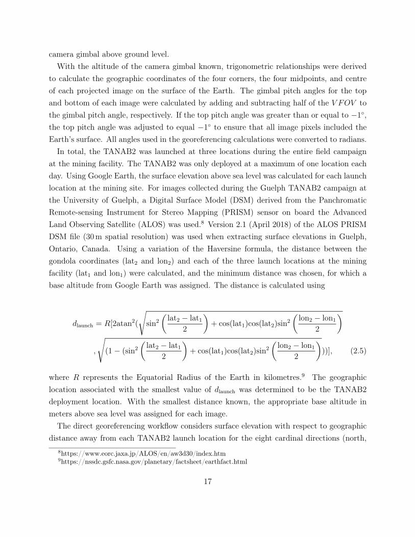
camera gimbal above ground level.With the altitude of the camera gimbal known, trigonometric relationships were derived

to calculate the geographic coordinates of the four corners, the four midpoints, and centreof each projected image on the surface of the Earth. The gimbal pitch angles for the topand bottom of each image were calculated by adding and subtracting half of the V FOV tothe gimbal pitch angle, respectively. If the top pitch angle was greater than or equal to −1◦,the top pitch angle was adjusted to equal −1◦ to ensure that all image pixels included theEarth’s surface. All angles used in the georeferencing calculations were converted to radians.

In total, the TANAB2 was launched at three locations during the entire field campaignat the mining facility. The TANAB2 was only deployed at a maximum of one location eachday. Using Google Earth, the surface elevation above sea level was calculated for each launchlocation at the mining site. For images collected during the Guelph TANAB2 campaign atthe University of Guelph, a Digital Surface Model (DSM) derived from the PanchromaticRemote-sensing Instrument for Stereo Mapping (PRISM) sensor on board the AdvancedLand Observing Satellite (ALOS) was used.8 Version 2.1 (April 2018) of the ALOS PRISMDSM file (30 m spatial resolution) was used when extracting surface elevations in Guelph,Ontario, Canada. Using a variation of the Haversine formula, the distance between thegondola coordinates (lat2 and lon2) and each of the three launch locations at the miningfacility (lat1 and lon1) were calculated, and the minimum distance was chosen, for which abase altitude from Google Earth was assigned. The distance is calculated using

dlaunch = R[2atan2(

√sin2

(lat2 − lat1

2

)+ cos(lat1)cos(lat2)sin2

(lon2 − lon1

2

)

,

√(1− (sin2

(lat2 − lat1

2

)+ cos(lat1)cos(lat2)sin2

(lon2 − lon1

2

)))], (2.5)

where R represents the Equatorial Radius of the Earth in kilometres.9 The geographiclocation associated with the smallest value of dlaunch was determined to be the TANAB2deployment location. With the smallest distance known, the appropriate base altitude inmeters above sea level was assigned for each image.

The direct georeferencing workflow considers surface elevation with respect to geographicdistance away from each TANAB2 launch location for the eight cardinal directions (north,

8https://www.eorc.jaxa.jp/ALOS/en/aw3d30/index.htm9https://nssdc.gsfc.nasa.gov/planetary/factsheet/earthfact.html

17

north-west, west, south-west, south, south-east, east, and north-east) and the line of sightfrom the camera for a given image pixel. Land surface elevation data in meters above sealevel for the eight cardinal directions up to 10 km away from each TANAB2 deploymentlocation at the mining facility, were obtained from the Geocontext-Profiler10 and saved asindividual text files. The camera gimbal Yaw angles were recorded in degrees positive clock-wise from north. If the Yaw angles were negative, 360◦ was added to the gimbal Yaw angle.Based on the Yaw angle of the camera gimbal and the base altitude, the appropriate file,containing data from the Geocontext-Profiler, was loaded into the Python script and a thirdorder polynomial was fitted to the data. Third order models have been used to representcurved Earth surfaces ([81]), such as those encountered in this mining facility.

The line of sight for a given image pixel was constructed by calculating the slope, whichis represented by the tangent of the pitch angle. For example, for the top centre pixel, thetangent of the top pitch angle is the slope of the line of sight for the top pixel, equal tothe TANAB2 altitude divided by the horizontal distance from the TANAB2 launch locationto where the line of sight intercepts the horizontal axis. This slope is negative because thecamera’s line of sight is always below the horizon.

From the derived third order polynomial for land surface elevation, the horizontal distancefrom the TANAB2 to where the image pixel is positioned was determined (dhoriz). The rootsof the intersection of the polynomial curve and the line of sight give the horizontal distance.If the roots were not real, the specific image was omitted from the ST calculation process.If multiple roots were found, the smallest real positive solution was chosen. For the miningfacility, if dhoriz was greater than 100 km, the pixel was omitted from the analysis. Likewise,for the Guelph campaign, if dhoriz was greater than 5 km, for the top centre and centre of animage especially, the pixel was omitted from the analysis. If the bottom centre of an imagehad a horizontal distance away from the TANAB2 above 5 km, the image was omitted fromthe analysis. This value was chosen as the TANAB2 was launched in an urban canyon aroundnumerous multi-story buildings where the camera line of sight likely would have intersectedan object at least 5 km away. This condition was implemented in the event the ALOS DSMfile spatial resolution did not fully consider building heights on the University of Guelphcampus. As a result, this filter value could be changed depending on the imaging location.

With the horizontal distance from the TANAB2 to where the image pixel is located known,the geographic coordinate pair for the corresponding horizontal (left to right) and vertical(top to bottom) pixel locations in the image were calculated using a variation of the Haversine

10http://www.geocontext.org/publ/2010/04/profiler/pl/

18

formula

Lat2 = asin[sin(Lat1)cos(dhorizR

)+ cos(Lat1)sin

(dhorizR

)cos(Yaw)] (2.6)

Lon2 = Lon1 + atan2([sin(Yaw)sin(dhorizR

)cos(Lat1)]

, [cos(dhorizR

)− sin(Lat1)sin(Lat2)]), (2.7)

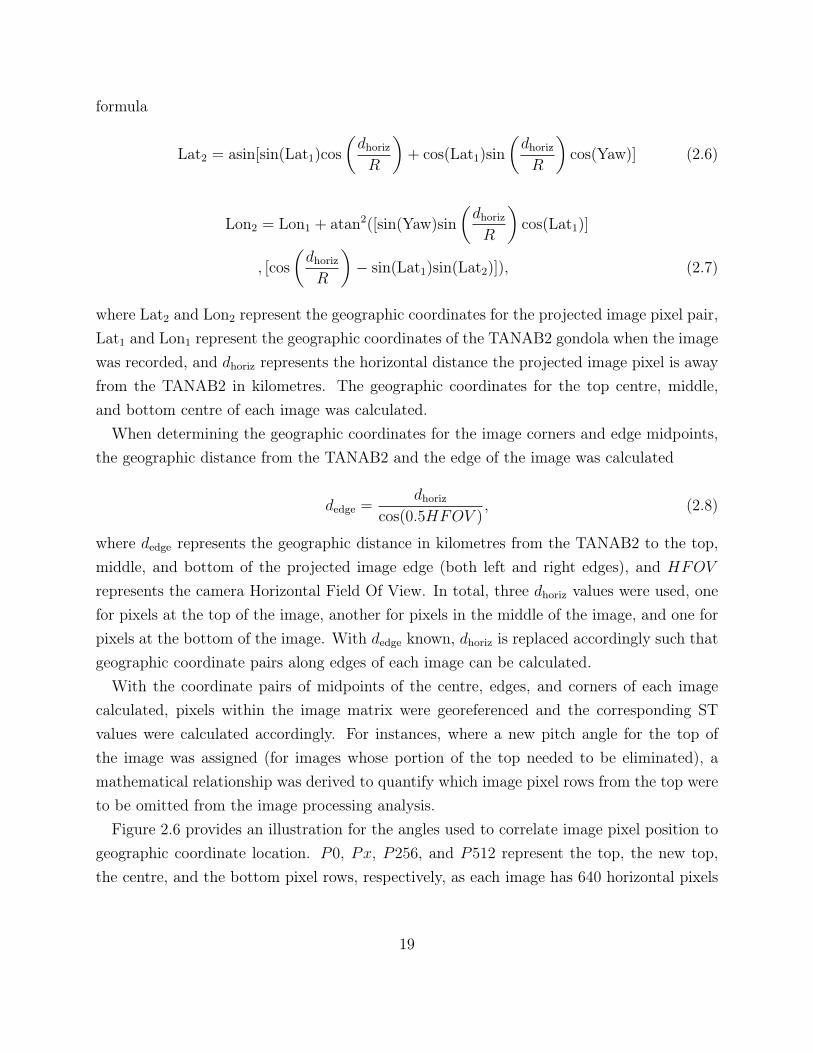
where Lat2 and Lon2 represent the geographic coordinates for the projected image pixel pair,Lat1 and Lon1 represent the geographic coordinates of the TANAB2 gondola when the imagewas recorded, and dhoriz represents the horizontal distance the projected image pixel is awayfrom the TANAB2 in kilometres. The geographic coordinates for the top centre, middle,and bottom centre of each image was calculated.

When determining the geographic coordinates for the image corners and edge midpoints,the geographic distance from the TANAB2 and the edge of the image was calculated

dedge =dhoriz

cos(0.5HFOV ), (2.8)

where dedge represents the geographic distance in kilometres from the TANAB2 to the top,middle, and bottom of the projected image edge (both left and right edges), and HFOV

represents the camera Horizontal Field Of View. In total, three dhoriz values were used, onefor pixels at the top of the image, another for pixels in the middle of the image, and one forpixels at the bottom of the image. With dedge known, dhoriz is replaced accordingly such thatgeographic coordinate pairs along edges of each image can be calculated.

With the coordinate pairs of midpoints of the centre, edges, and corners of each imagecalculated, pixels within the image matrix were georeferenced and the corresponding STvalues were calculated accordingly. For instances, where a new pitch angle for the top ofthe image was assigned (for images whose portion of the top needed to be eliminated), amathematical relationship was derived to quantify which image pixel rows from the top wereto be omitted from the image processing analysis.

Figure 2.6 provides an illustration for the angles used to correlate image pixel position togeographic coordinate location. P0, Px, P256, and P512 represent the top, the new top,the centre, and the bottom pixel rows, respectively, as each image has 640 horizontal pixels

19

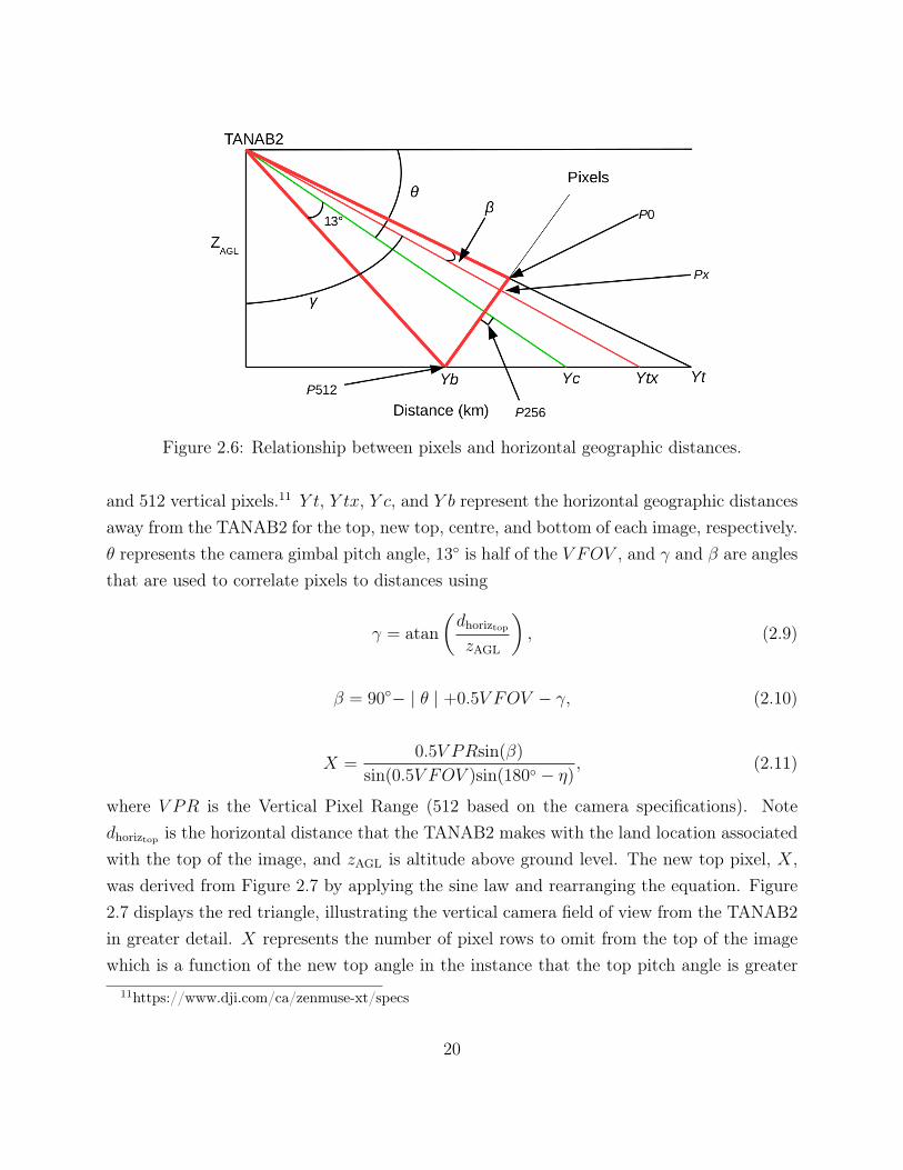
Figure 2.6: Relationship between pixels and horizontal geographic distances.

and 512 vertical pixels.11 Y t, Y tx, Y c, and Y b represent the horizontal geographic distancesaway from the TANAB2 for the top, new top, centre, and bottom of each image, respectively.θ represents the camera gimbal pitch angle, 13◦ is half of the V FOV , and γ and β are anglesthat are used to correlate pixels to distances using

γ = atan(dhoriztopzAGL

), (2.9)

β = 90◦− | θ | +0.5V FOV − γ, (2.10)

X =0.5V PRsin(β)

sin(0.5V FOV )sin(180◦ − η), (2.11)

where V PR is the Vertical Pixel Range (512 based on the camera specifications). Notedhoriztop is the horizontal distance that the TANAB2 makes with the land location associatedwith the top of the image, and zAGL is altitude above ground level. The new top pixel, X,was derived from Figure 2.7 by applying the sine law and rearranging the equation. Figure2.7 displays the red triangle, illustrating the vertical camera field of view from the TANAB2in greater detail. X represents the number of pixel rows to omit from the top of the imagewhich is a function of the new top angle in the instance that the top pitch angle is greater

11https://www.dji.com/ca/zenmuse-xt/specs

20

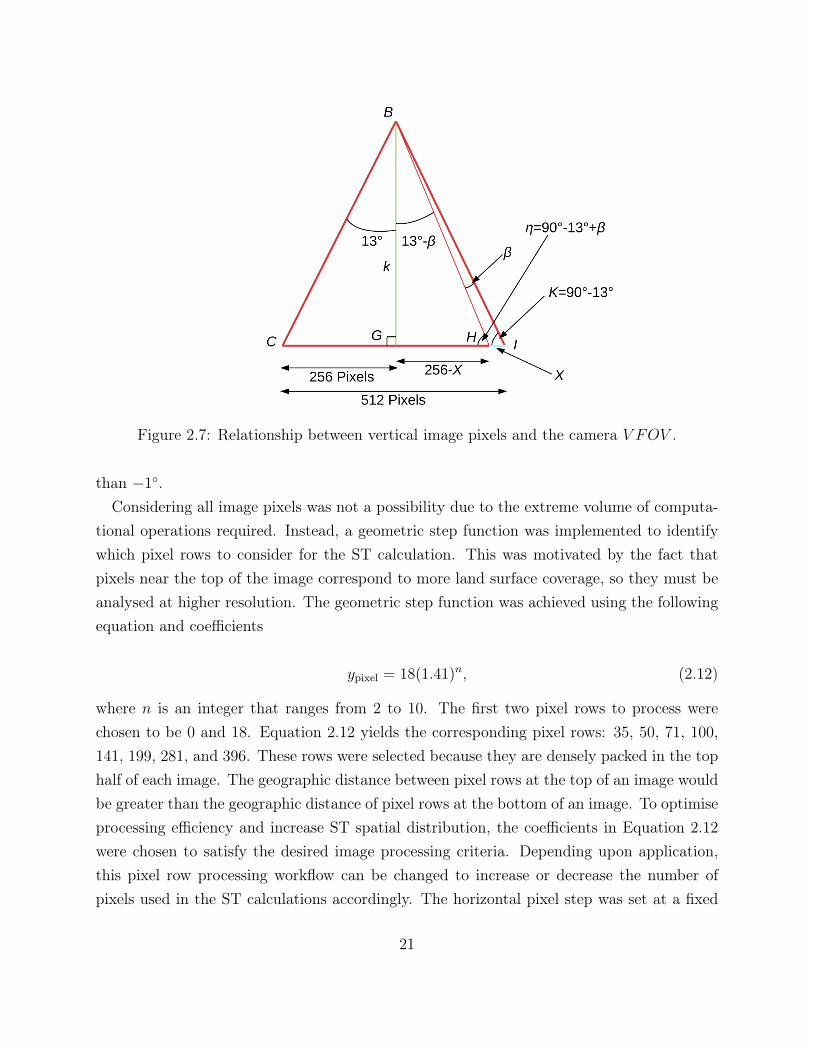
Figure 2.7: Relationship between vertical image pixels and the camera V FOV .

than −1◦.Considering all image pixels was not a possibility due to the extreme volume of computa-

tional operations required. Instead, a geometric step function was implemented to identifywhich pixel rows to consider for the ST calculation. This was motivated by the fact thatpixels near the top of the image correspond to more land surface coverage, so they must beanalysed at higher resolution. The geometric step function was achieved using the followingequation and coefficients

ypixel = 18(1.41)n, (2.12)

where n is an integer that ranges from 2 to 10. The first two pixel rows to process werechosen to be 0 and 18. Equation 2.12 yields the corresponding pixel rows: 35, 50, 71, 100,141, 199, 281, and 396. These rows were selected because they are densely packed in the tophalf of each image. The geographic distance between pixel rows at the top of an image wouldbe greater than the geographic distance of pixel rows at the bottom of an image. To optimiseprocessing efficiency and increase ST spatial distribution, the coefficients in Equation 2.12were chosen to satisfy the desired image processing criteria. Depending upon application,this pixel row processing workflow can be changed to increase or decrease the number ofpixels used in the ST calculations accordingly. The horizontal pixel step was set at a fixed

21

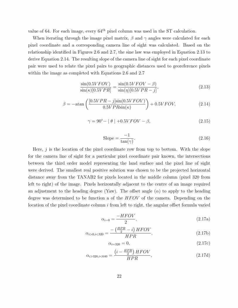
value of 64. For each image, every 64th pixel column was used in the ST calculation.When iterating through the image pixel matrix, β and γ angles were calculated for each

pixel coordinate and a corresponding camera line of sight was calculated. Based on therelationship identified in Figures 2.6 and 2.7, the sine law was employed in Equation 2.13 toderive Equation 2.14. The resulting slope of the camera line of sight for each pixel coordinatepair were used to relate the pixel pairs to geographic distances used to georeference pixelswithin the image as completed with Equations 2.6 and 2.7

sin(0.5V FOV )

sin(κ)[0.5V PR]=

sin(0.5V FOV − β)

sin(η)[0.5V PR− j], (2.13)

β = −atan(

[0.5V PR− j]sin(0.5V FOV )

0.5V PRsin(κ)

)+ 0.5V FOV, (2.14)

γ = 90◦− | θ | +0.5V FOV − β, (2.15)

Slope =−1

tan(γ). (2.16)

Here, j is the location of the pixel coordinate row from top to bottom. With the slopefor the camera line of sight for a particular pixel coordinate pair known, the intersectionsbetween the third order model representing the land surface and the pixel line of sightwere derived. The smallest real positive solution was chosen to be the projected horizontaldistance away from the TANAB2 for pixels located in the middle column (pixel 320 fromleft to right) of the image. Pixels horizontally adjacent to the centre of an image requiredan adjustment to the heading degree (Yaw). The offset angle (α) to apply to the headingdegree was determined to be function a of the HFOV of the camera. Depending on thelocation of the pixel coordinate column i from left to right, the angular offset formula varied

αi=0 =−HFOV

2, (2.17a)

αi>0,i<320 =−(HPR

2− i)HFOV

HPR, (2.17b)

αi=320 = 0, (2.17c)

αi>320,i<640 =

(i− HPR

2

)HFOV

HPR, (2.17d)

22

αi=640 =HFOV

2, (2.17e)

where HPR represents the Horizontal Pixel Range (640 pixels based on the physical cameraspecifications). The Yaw heading of the camera gimbal corresponded to the middle of theimage. As a result the heading for any pixels to the left of the centre of the image requiredthe angular offset to be removed from the recorded Yaw. Likewise, any pixels to the right ofthe image required the angular offset to be added to the recorded Yaw. In cases where theaddition of the angular offset to the heading angle resulted in a negative value or a valuegreater than 2π radians, then 2π radians were either added or subtracted, respectively, toensure that only positive angles between 0 and 2π radians were passed to Equations 2.6 and2.7.

The code for the direct georeferencing method is included in Sections A.2.4 and A.3.4 forthe mining facility and the Guelph campaigns.

2.3.2 Thermal Camera Calibration

Using ExifTool and ImageMagick, recorded signal values from individual pixels were ex-tracted and saved to a matrix in the Python script. These raw signal values were convertedto surface temperatures considering a variation of Planck’s Law.

Due to field conditions and physical limitations encountered at the mining facility, errorsintroduced from reflections and transmission could not be accounted for. However, thethermal camera used in the field campaign was calibrated in a pre-field outdoors experimenton campus at the University of Guelph, Guelph, Ontario, Canada. Three radiometric imageswere captured roughly thirty seconds apart for every hour between 06:00 and 23:00 EDTover two consecutive days. The thirty second time interval was selected as Olbrycht andWięcek [69] noted that uncooled thermal cameras can experience temperature drift up to1 K per minute if a radiometric calibration was not recently completed. Four different landsurface types were imaged including water, soil, grass, and developed land (urban surfaces).Each image included a certified thermometer which measured the corresponding land surfacetemperature as recorded by the image.

Surface temperatures from the top of the thermometer were calculated from the thermalimages using FLIR Tools. For each hourly image set, the average of the surface temperaturesderived in FLIR Tools was calculated and used to calibrate the R, B, O, and F constantsaccordingly, where R = R1

R2. The temperatures recorded by the certified thermometer were

scaled to adjust for the test location’s height above sea level (334 m for Guelph, Ontario,

23

Canada). For the thermal image temperatures, (UObj) was calculated from Equation 2.18.

UObj =R

exp(

BTObj

)− F

−O, (2.18)

where UObj represents the radiative energy emitted from the imaged object, TObj representsthe surface temperature of the imaged object derived from FLIR Tools, R represents theuncooled camera response, B is a constant related to Planck’s radiation law, F relates to thenon-linear response of the thermal imaging system, and O represents an offset [12]. Equation2.18 can be rearranged to calculate TObj as per Equation 2.19.

TObj =B

ln(

RUObj+O

+ F) . (2.19)

The R, B, O, and F constants used to calculate the UObj value were the default constantsstored in the metadata of each thermal image. The default constants and calibrated constantsare displayed in Table 2.3.

Using the empirical line method, described by Smith and Milton [85], the UObj values andthe corresponding certified thermometer temperatures were plotted against each other tocalibrate the constants used in Equation 2.19 as a function of land surface type. The figuresillustrating the empirical line method are displayed in Figure 2.8. The Non-Linear Least-Squares Minimization and Curve-Fitting (LMFIT) of Python library version 0.9.1312 wasused with Equation 2.19 to fit and optimise the camera constants while minimising residualsfor each specific land surface type.

Using the LMFIT library to fit camera constants for each land surface ultimately reducedthe bias and RMSE values when compared to the default camera constants shown in Table2.4. Using the calibrated constants for the calculation of land ST at the mining facilityimproved accuracy of the measurement. These findings are comparable to Gallardo-Saavedraet al. [27] who reported that the manufacturer stated accuracy of the FLIR Vue Pro R 640,Tau 2 640, and Zenmuse XT 640 was ±5 K. Similarly, Kelly et al. [46] used the empiricalline calibration method for a FLIR Vue Pro 640 uncooled thermal camera and quantified theaccuracy of the camera to be ±5 K.

The Python code used to calculate the calibrated camera constants and the plots in Figure2.8, are located in Sections A.1 and A.1.1 respectively.

12https://lmfit.github.io/lmfit-py/index.html

24

(a) Default and calibrated temperature for water. (b) Default and calibrated temperature for soil.

(c) Default and calibrated temperature for devel-oped land. (d) Default and calibrated temperature for grass.

Figure 2.8: Certified temperature compared to radiometric image pixel signal value for water,soil, developed land, and grass.

25

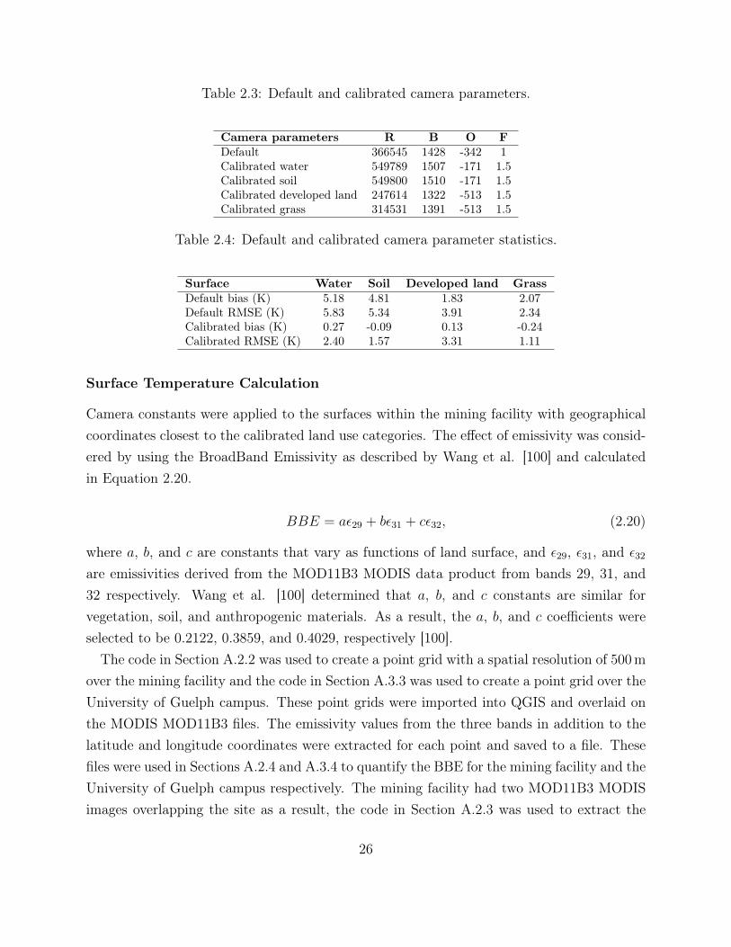
Table 2.3: Default and calibrated camera parameters.

Camera parameters R B O FDefault 366545 1428 -342 1Calibrated water 549789 1507 -171 1.5Calibrated soil 549800 1510 -171 1.5Calibrated developed land 247614 1322 -513 1.5Calibrated grass 314531 1391 -513 1.5

Table 2.4: Default and calibrated camera parameter statistics.

Surface Water Soil Developed land GrassDefault bias (K) 5.18 4.81 1.83 2.07Default RMSE (K) 5.83 5.34 3.91 2.34Calibrated bias (K) 0.27 -0.09 0.13 -0.24Calibrated RMSE (K) 2.40 1.57 3.31 1.11

Surface Temperature Calculation

Camera constants were applied to the surfaces within the mining facility with geographicalcoordinates closest to the calibrated land use categories. The effect of emissivity was consid-ered by using the BroadBand Emissivity as described by Wang et al. [100] and calculatedin Equation 2.20.

BBE = aε29 + bε31 + cε32, (2.20)

where a, b, and c are constants that vary as functions of land surface, and ε29, ε31, and ε32are emissivities derived from the MOD11B3 MODIS data product from bands 29, 31, and32 respectively. Wang et al. [100] determined that a, b, and c constants are similar forvegetation, soil, and anthropogenic materials. As a result, the a, b, and c coefficients wereselected to be 0.2122, 0.3859, and 0.4029, respectively [100].

The code in Section A.2.2 was used to create a point grid with a spatial resolution of 500 m

over the mining facility and the code in Section A.3.3 was used to create a point grid over theUniversity of Guelph campus. These point grids were imported into QGIS and overlaid onthe MODIS MOD11B3 files. The emissivity values from the three bands in addition to thelatitude and longitude coordinates were extracted for each point and saved to a file. Thesefiles were used in Sections A.2.4 and A.3.4 to quantify the BBE for the mining facility and theUniversity of Guelph campus respectively. The mining facility had two MOD11B3 MODISimages overlapping the site as a result, the code in Section A.2.3 was used to extract the

26

emissivity band data from the original satellite images. This problem was not encounteredfor the Guelph field campaign.

The total signal (UTot) recorded by the uncooled thermal camera can be separated intothree components as in Equation 2.21. The first component represents the radiative energyemitted from the imaged object (UObj), the second component represents the reflected energyfrom the imaged object (URefl), and the third component accounts for the radiative energytransmitted from the atmosphere (UAtm). ε represents the emissivity of the surface andis accounted for by Equation 2.20 and τ represents the transmissivity of the atmospherewhose value is generally close to 1.0 [93]. As a result, only the radiative energy reflectedand emitted from the imaged object are considered in Equation 2.21, where to retrieve UObj

and subsequently TObj, URefl is removed from UTot. The calibration of camera constants wascompleted to correct for incoming reflected radiation via

UTot = ετUObj + τ(1− ε)URefl + (1− τ)UAtm. (2.21)

These calculations are detailed in Sections A.2.4 and A.3.4 corresponding to the miningfacility and the Guelph campaign. On average, it takes 17.8 seconds to directly georeferenceand calculate surface temperature from one image.

2.4 Principal Component Analysis (PCA)

In order to determine the geographical direction for which one has the largest variationsin surface temperature, a PCA was performed. PCA is a very well-known approach foranalysing data (especially large data) to deduce meaningful conclusions about it. The prin-ciple behind PCA lies in the fact that it can mathematically determine the principal com-ponents (eigenvectors) showing the directions of the largest deviations in the data; for moreinformation about PCA see for instance the work of Jolliffe [42]. Note that this method givesthe main axes along which the variations in the data are the largest. In this analysis, it wasof interest to find the direction of the land surface for which the temperature gradient wasthe largest. Therefore, the axis that had the most variation was picked and the results wereanalysed accordingly. PCA was completed for six four-hour time intervals.

The Python code created to calculate and plot the PCA is located in Section A.2.8.

27

Chapter 3

Results and Discussion

3.1 Mining Site Campaign

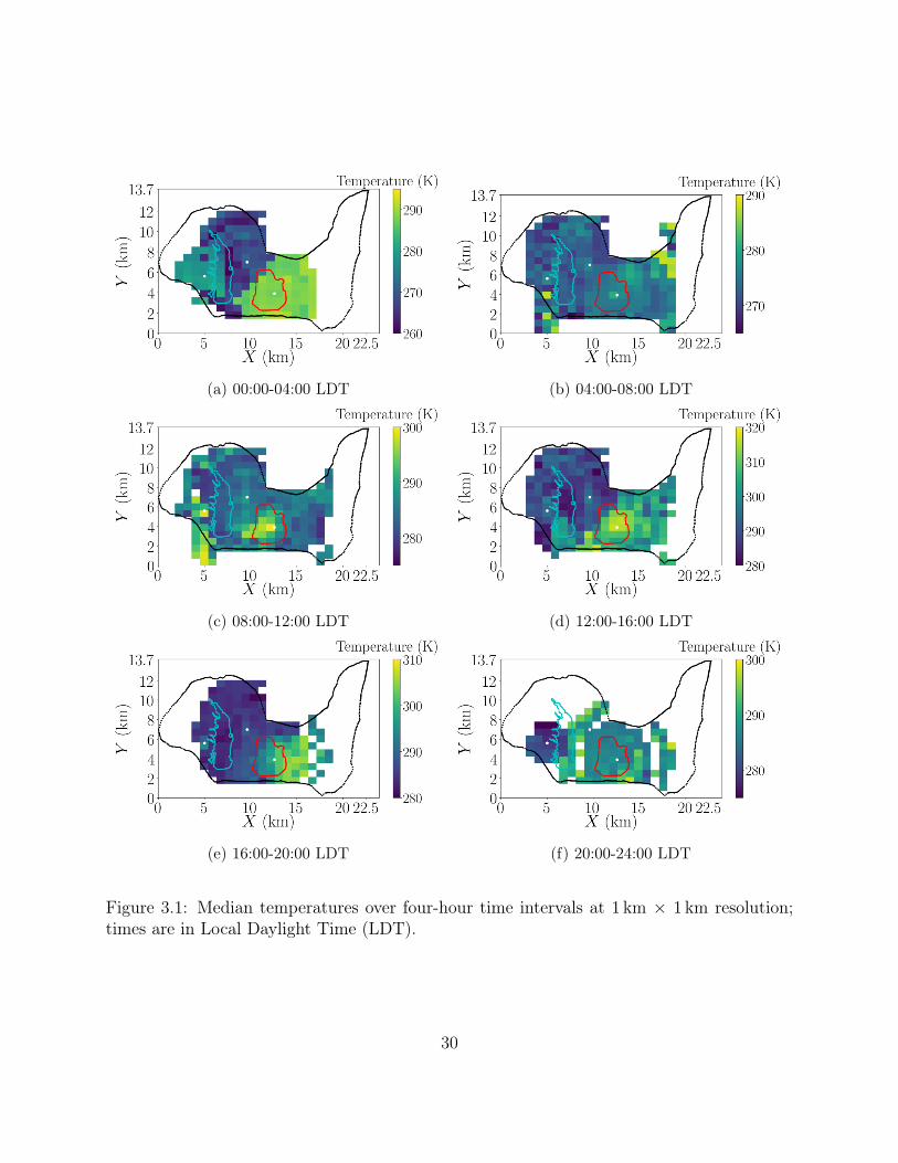
Three analyses were conducted on the processed image data. The first analysis representsmedian ST distribution at a spatial resolution of 1 km × 1 km derived from images recordedover the entire length of the field campaign. In total, six four-hour time intervals in LocalDaylight Time (LDT) (00:00-04:00 LDT, 04:00-08:00 LDT, 08:00-12:00 LDT, 12:00-16:00LDT, 16:00-20:00 LDT, and 20:00-24:00 LDT) representing ST for the entire field campaignwere produced highlighting diurnal ST variation with respect to the mining facility bound-ary, the mine, and the tailings pond as displayed in Figure 3.1. Corresponding box plotsrepresenting the temperature variation of the mine and tailings pond are also included foreach time interval as per Figure 3.2. For each survey, on average 1910 images were used foreach four-hour time interval.

The second analysis focuses on comparing the calculated ST derived from the images col-lected on May 24, 2018 over the 12:00-14:00 LDT time interval with respect to the MODISMOD11A1 image recorded during the early afternoon on May 24, 2018. Three plots werecreated (as per Figure 3.3) including the ST spatial distribution map at 1 km × 1 km resolu-tion derived from the workflow, the MOD11A1 dataset for each corresponding ST tile, andthe absolute error for each tile is included.

The third analysis focuses on identifying horizontal direction of the highest surface tem-perature variances. The direction with the highest surface temperature variances for eachtime interval was calculated from the images collected during the field campaign by complet-ing a PCA on the data derived from each time interval. The results are presented in Figure3.4.

28

The code used to separate the data into six four-hour intervals is included in Section A.2.5,the code to correct surface temperatures as a function of land material type is included inSection A.2.6, and the code used to create the surface temperature maps and box plots isincluded in Section A.2.7.

3.1.1 Diurnal Surface Temperature

Surface temperature maps with a spatial resolution of 1 km × 1 km for the entire miningfacility at six four-hour time intervals are displayed in Figure 3.1. These plots were createdby calculating the median temperature for all data recorded within each time interval overthe entire field campaign within a 1 km × 1 km area (tile). The axes represent distance inkilometres and the colour bar represents surface temperature in Kelvin.

Box plots (Figure 3.2) representing the surface temperature range in Kelvin of the twokey geographical features of the mining facility, the mine, and the tailings pond, at thecorresponding six four-hour time intervals were created to compare diurnal ST variation.The ST values included in the box plot are located within the red and teal perimeters ofthe mine and tailings pond, respectively, shown in Figure 2.2. The black circles representtemperature values outside of the 95th and 5th percentiles. The upper black line and lowerblack line of the box plot correspond to the 95th and 5th percentiles. The middle orange linerepresents the median surface temperature of each geographical feature.

During the 00:00-04:00 LDT time interval, there was a distinct temperature gradientbetween the mine, the land west of the pond, and the pond itself. This gradient is furtherquantified by the corresponding box plot where the median surface temperature gradientbetween the two surface features was approximately 20 K.

There was a clear surface temperature gradient between the mine and the pond duringthe 04:00-08:00 LDT time interval. However, the magnitude of the temperature gradientbetween the mine and the pond was the lowest during this time period. Both the surfacetemperature map and the box plot display this trend as this time interval includes imagescaptured during and after sunrise.

Over the 08:00-12:00 LDT interval, the surface temperatures of both the mine and thepond increase. Likewise, the temperature gradient between the two land surface featuresalso grows, where the mine’s surface temperature is higher than the tailings pond surfacetemperature.

During the 12:00-16:00 LDT interval, an apparent temperature gradient existed between

29

(a) 00:00-04:00 LDT (b) 04:00-08:00 LDT

(c) 08:00-12:00 LDT (d) 12:00-16:00 LDT

(e) 16:00-20:00 LDT (f) 20:00-24:00 LDT

Figure 3.1: Median temperatures over four-hour time intervals at 1 km × 1 km resolution;times are in Local Daylight Time (LDT).

30

(a) 00:00-04:00 LDT (b) 04:00-08:00 LDT

(c) 08:00-12:00 LDT (d) 12:00-16:00 LDT

(e) 16:00-20:00 LDT (f) 20:00-24:00 LDT

Figure 3.2: Box plots representing temperature distribution over four-hour time intervals forthe tailings pond and mine, where the orange line is the median temperature; times are inLocal Daylight Time (LDT).

31

the tailings pond and the mine. The area to the north-west of the mine had a lower surfacetemperature as compared to areas south and east of the mine.

The variability of surface temperatures between the mine and the pond decreased over the16:00-20:00 LDT interval. Although a clear temperature gradient was present, the box plotdisplays a narrower temperature range as compared to most other time intervals.

The same temperature gradient as discussed during other time periods occurs within the20:00-24:00 LDT period. There are a few data gaps for ST north-west of the mine as theTANAB2 was deployed less during these hours compared to other time periods. Nonetheless,the west side of the pond possesses a lower surface temperature as compared to the mine itself.The overall surface temperature magnitude for both land surface features was determinedto be decreasing during this interval, after sunset.

3.1.2 Satellite Comparison

On May 24, 2018 MODIS on the Terra satellite imaged the remote mining site during theearly afternoon. The TANAB2 was launched within the mine between 12:00 and 14:00 LDTon the same date. Figure 3.3 displays the surface temperatures recorded by the thermal cam-era from the TANAB2, the surface temperatures recorded by MODIS from the MOD11A1dataset, and the absolute error between the two datasets.

Absolute error with respect to MODIS temperatures on May 24, 2018 was calculatedand the spatial distribution of temperature bias is displayed in Figure 3.3. The maximum,minimum, and median absolute error were calculated to be 14.3 K, −12.2 K, and 0.64 K,respectively. The bias and RMSE were determined to be 0.5 K and 5.45 K, respectively.Furthermore, it was noted that the absolute error increased north-west of the mine, towardsthe pond. This likely occurred as the TANAB2 was launched within the mine, below gradelevel (with respect to the mining facility), while the land elevation increases north-west ofthe mine towards the tailings pond. With this change in elevation, the calculated surfacetemperatures northwest of the mine are estimated from very oblique angle images, possiblycontributing to the increased error. In addition, that region contains very localised hot spots,such as pipelines, that are beyond MODIS data product resolutions to be detected by thesatellite but within the resolution of the thermal images in the current method. This canalso explain the discrepancy between the methods. On the other hand, the elevation of theland surface decreased south and east of the mine. This decrease is likely attributed to lessoblique images and therefore lower absolute error between the two datasets. Nevertheless,

32

(a) Thermal camera ST (b) MODIS ST

(c) Absolute error in ST

Figure 3.3: Comparison between the developed thermal imaging method, the MODISMOD11A1 dataset, and absolute error between the two methods; (a) median ST from May24, 2018 12:00-14:00 LDT as recorded by the thermal camera at a 1 km × 1 km resolution;(b) daytime temperatures captured by MODIS recorded during the early afternoon on May24, 2018 and derived from the MOD11A1 dataset at a 1 km × 1 km resolution; (c) absoluteerror between the two methods at a 1 km × 1 km resolution; times in Local Daylight Time(LDT).

33

the localised warm regions of surface temperatures within the mine and east of the minerecorded by MODIS were also captured from the thermal images as displayed by the surfacetemperature plots in Figure 3.3.

The increase in error between the mine and the pond can be accounted for from the rapidchange in topography. In this region, the bottom of the mine pit is approximately 100 m

into the earth. Conversely, the area directly to the east of the pond (the levee) is the highestlocation of the entire site. The total change of land surface elevation between the mine andthe pond is very significant and may not be fully considered by the Digital Elevation Model(DEM) acquired from Google Earth. Wang et al. [101] evaluated the accuracy of elevationdata provided by Google Earth for over 20,000 locations of the conterminous United States.They determined that the mean average error, RMSE, and bias of elevation was 10.72 m,22.31 m, and 0.13 m, respectively. Based on Wang et al. [101], Google Earth accuracy variessignificantly by location. Furthermore, since the landscape of the mining facility is changingrapidly, the use of the Google Earth elevation data likely introduces further error into themethod. For more accurate results, sUAS-based Light Detection And Ranging (LiDAR)could be a feasible solution, especially in areas where high time resolution data is requiredor very high resolution satellite imagery capable of creating elevation models is required[3, 29, 67].

Further improvement of the imaging workflow may also reduce errors. The imaging methodonly considers elevation profiles for the eight cardinal directions of each TANAB2 launch site.Using a high spatial resolution DEM raster and QGIS, the elevation profile for individualimages could be quantified programmatically in Python. The elevation profiles for individualpixels within the image could also be quantified using this method. However, the accuracyof this method is dependent upon the accuracy and resolution of the DEM data source.Nonetheless, the accuracy of the Google Earth elevation data was deemed to be acceptablefor this application.

Using oblique and very oblique images in the method may have contributed to surface tem-perature error even with using the corrected camera parameters R, B, O, and F . Obliqueimaging is known to affect observed surface temperatures as a function of camera pitch an-gle [22]. Increasingly oblique imaging angles can result in a higher proportion of reflectedradiation and more varied emissivity values over waterbodies [5, 22, 90]. The proportion ofwaterbodies within the mining facility is low and even the tailings pond may not truly berepresentative of a pond due to byproducts introduced from the mine ore extraction process.It is known that imaging angles higher than 30◦ of nadir can affect surface temperature by

34

0.5 K [22, 45, 90]. For land surfaces, James et al. [40] recorded lava flows with ±3 % radia-tive power differences. The areas with the highest temperature error were not waterbodies.Oblique images of land surfaces likely have less impact on emissivity as opposed to imagesof water bodies. Nonetheless, the presence of this error source is acknowledged in this the-sis. Additionally, the processing of oblique and very oblique images may have introducedgeoreferencing (positioning) error into the quantified pixel latitude and longitude values, es-pecially for the upper half of each image. Pixel rows at the top of each image are increasinglyfurther away from each other as compared to pixel rows at the bottom of an image. As aresult, georeferenced pixels near the top of oblique images may not fully consider surfaceterrain variation, thus leading to increased positioning errors. Since the direct evaluation ofthe georeferencing method was not evaluated, quantitative impact of these potential errorscannot be fully determined.

Other than surface elevation variation, calculated temperature errors may have been in-troduced from the camera constant calibration completed in Guelph, Ontario, Canada. Thesurface materials at the mining site may have been different as opposed to the tested surfacetemperatures recorded during the calibration experiment. The difference in physical prop-erties may have contributed to the increased minimum and maximum errors of −12.2 K and14.3 K, respectively. However, the overall median error was calculated to be 0.64 K which issignificantly below the manufacturer reported accuracy of ± 5 K and the calibrated accuracyof a FLIR Vue Pro 640 of ± 5 K [27, 46]. These elevated maximum and minimum errors maybe due to highly oblique images, near horizontal, where reflected radiation can significantlyimpact the radiometric measurement. To avoid these errors, deploying the TANAB2 at ahigher altitude would be necessary to reduce oblique imaging angles. However, this was notpossible as the TANAB2 profile height was predetermined from aviation and site specificregulations.

Certain parameters (such as filtering angles or calculated distances away from the TANAB2)included in the direct georeferencing and temperature calculation code could be changedand a sensitivity analysis could be performed. It is possible to reduce errors through thecompletion of sensitivity analyses on all relevant parameters. The benefits and drawbacksassociated with changing these parameters would need to be considered before new valuesare selected. For example, omitting very oblique images would reduce the area of coveredby the surface temperature maps but the errors associated with reflected radiation may beminimised. The developed image processing method is very customisable depending on thedesired application.

35

3.1.3 Principal Component Analysis (PCA)

Figure 3.4: Representative horizontal directions encompassing the mining facility whichdisplay the largest surface temperature variation for each time interval; times are in LocalDaylight Time (LDT).

The result of the PCA analysis is shown in Figure 3.4. As can be seen, the highest surfacetemperature variation is the north-west-south-east direction. Referring to Figure 2.2, thenorth-west-south-east direction intersects the mine and processing facilities to the south-eastand the pond and forest, beyond the facility, to the north-west. This surface temperaturevariation was present in each time interval, especially during 00:00-04:00 LDT, 04:00-08:00LDT, and 16:00-20:00 LDT, where the normalised PCA horizontal directions are close tooverlapping each other.

36

3.2 Guelph Campaign

One analysis was conducted on the images collected during the University of Guelph Summer2018 field campaign. Diurnal median ST distribution was calculated from the images col-lected on July 28, 2018 and August 13, 2018 over a 1 km × 1 km study area of the Universityof Guelph campus. Surface temperature plots were created at two spatial resolutions, 20 m

× 20 m and 50 m × 50 m, respectively. In total, five ST plots were created representing ReekWalk and the land surrounding the TANAB2 launch site for 04:00-08:00 Eastern DaylightTime (EDT), 08:00-12:00 EDT, 12:00-16:00 EDT, 16:00-20:00 EDT, and 20:00-24:00 EDT.Additional landmarks were identified in Figures 3.5 and 3.6.

For each plot in Figure 3.5, differing median ST patterns exist in relation to urban surfacesand green spaces on and around the University of Guelph campus. Although Figure 3.6represents ST at a lower spatial resolution, the median ST distribution follows a similartrend as depicted in Figure 3.5.

During the 04:00-08:00 EDT interval, the area to the bottom left of the TANAB2 launchsite was cooler as compared to other regions. This area consists of green space mixed withurban surfaces. The green space could have contributed to lower surface temperatures. Thearea at the bottom right of the plot has higher median ST values as compared to the bottomleft region. The area to the bottom right primarily consists of a built-up residential areawhich may contribute to the increased temperatures. The upper right region in relation tothe TANAB2 launch location is The Arboretum at University of Guelph, which primarilyconsists of trees and green space. The top right of the plot (The Arboretum) appears tohave higher median ST values as compared the green space to the bottom right of thelaunch. These higher median ST values may be influenced by errors attributed to highlyoblique imaging angles where the ST calculation does not account for the increased fractionof reflected or transmitted radiation [33, 40].

During the 08:00-12:00 EDT interval, urban surfaces had higher median ST values as com-pared to green spaces. Furthermore, this time range had a greater ST range and increasinglynon-uniform temperature variations as compared to the 04:00-08:00 EDT interval. Thesetrends may be developed as the sunrise for nearby Hamilton, Ontario, Canada was 06:06EDT on July 28, 2018 and 06:23 EDT on August 13, 2018.1 Chudnovsky et al. [16] notedthat the minimal surface temperature values occurred immediately before sunrise. As aresult, with approximately only two hours of influent solar radiation, the 04:00-08:00 EDT

1https://www.nrc-cnrc.gc.ca/eng/services/sunrise/index.html

37

interval should be cooler than the 08:00-12:00 EDT plot with four hours of increasinglyintense solar radiation.

Over the 12:00-16:00 EDT interval, the trend of increasing surface temperatures continuewith respect to the 08:00-12:00 EDT interval. The plot represents median ST for middayand afternoon, which is commonly one of the intervals with the highest land surface temper-atures. Highly urbanized surfaces, such as parking lots, especially in close proximity to theTANAB2 launch site, had the highest median surface temperatures. Furthermore, campusbuildings generally had higher ST values as compared to their surroundings. This trend isespecially true for the Edmund C. Bovey Building, the Albert A. Thornbrough Building,the Crop Science Building, the Fieldhouse, and the Athletic Centre. Johnston Green andthe residential area at the bottom right of the launch site, had cooler temperatures as com-pared to the rest of the ST plot. Outside of these specific landmarks, the median surfacetemperature distribution is rather uniform within the 290 K to 300 K range.

The urban surfaces of the University of Guelph campus had increased surface temperaturesas compared to the other areas in the 12:00-16:00 EDT interval. Specifically, areas to theright of the TANAB2 launch site had the highest ST, including the Athletic Centre, theGryphon Centre Arena, the Crop Science Building, the Landscape Architecture Building,and Rozanski Hall. The region to the far right and bottom right of Reek Walk also had highersurface temperatures within the residential area. Urbanized areas with mixed green spacehad generally uniform surface temperatures within the 290 K to 300 K range. Furthermore,the far top left region of the plot had cooler surface temperatures as compared to other areas.The Cutten Fields golf course and the University of Guelph North Residences, intermixedwith green spaces, are situated in the region.

The spatial pattern of ST where green spaces have lower ST compared to urbanized areashas been reported in literature [108]. In nearby Hamilton, Ontario, Canada on July 28,2018, the sunset occurred at 20:46 EDT and 20:26 EDT on July 28, 2018 and August 13,2018, respectively. The 16:00-20:00 EDT interval was the last time range with continualincoming solar radiation. The time period with the highest ST values varies by location.Urban ST is known to be highly influenced by the height and width of buildings, streetorientation, building and street orientation, and the sky view factor of the location [2].The time interval with the highest surface temperatures was calculated to be the 16:00-20:00 EDT period. However Ahmed et al. [2] conducted a study which determined thatbuilding roof temperatures achieved a maximum at noon and building wall and sidewalksurface temperatures reached a maximum later in the afternoon. As a result, urban surface

38

temperature trends cannot be generalised.The surface temperature values decrease between the 16:00-20:00 EDT and the 20:00-24:00

EDT intervals. Without incoming solar radiation, object surfaces have a net radiative lossand ultimately possess lower surface temperatures values. The highest surface temperaturesoccur at the bottom right and top right regions of the plot, in the residential area andThe Arboretum respectively. Additionally, the parking lots to the right of the TANAB2launch, Johnston Hall, and McLaughlin library had higher temperatures as opposed to otherbuildings and regions. The lowest ST values were located at the bottom left of the plot,adjacent to the University of Guelph Equine Sport & Reproduction Center. However, surfacetemperatures near the edges of this plot may be influenced by highly oblique images wherethe fraction of reflected and transmitted radiation is higher than the values used in the STcalculation.

Surface temperature plots were created at two spatial resolutions, 20 m × 20 m, and 50 m

× 50 m. Although the 20 m spatial resolution figures provide more detail, the 50 m spatialresolution plots may be more useful for analysis. Due to the nature of the image processingmethod, pixels in the same vertical rows are selected for each image. In the event wheremore images are recorded during a particular TANAB2 profile, surface temperatures fromthe same region would be calculated. This process would result in concentric-like circles oftemperature gradients. In Figure 3.5, concentric-like surface temperature patterns appear forall time periods. Conversely, the 50 m spatial resolution temperature plots do not have anynoticeable concentric temperature patterns. With a lower spatial resolution, the quantifiedmedian temperature for each square is large enough to omit spatial temperature distributioneffects imposed from the image processing workflow.

The code used to separate the data into the five four-hour time intervals is included inSection A.3.5 and the code used to calculate surface temperatures as a function of landmaterial type and to plot the surface temperature maps is included in Section A.3.6.

39

(a) 04:00-08:00 EDT (b) 08:00-12:00 EDT

(c) 12:00-16:00 EDT (d) 16:00-20:00 EDT

(e) 20:00-24:00 EDT

Figure 3.5: Median surface temperatures over four-hour time intervals at 20 m × 20 m spa-tial resolution, where the red dot represents the TANAB2 launch location (Reek Walk), theblack circle represents the Gryphon Centre Arena, the magenta circle represents the Uni-versity Centre, the blue circle represents the Athletic Centre, the yellow circle representsVarsity Field, the cyan circle represents Johnston Green, and the white circle represents theFieldhouse.

40

(a) 04:00-08:00 EDT (b) 08:00-12:00 EDT

(c) 12:00-16:00 EDT (d) 16:00-20:00 EDT

(e) 20:00-24:00 EDT

Figure 3.6: Median surface temperatures over four-hour time intervals at 50 m × 50 m spa-tial resolution, where the red dot represents the TANAB2 launch location (Reek Walk), theblack circle represents the Gryphon Centre Arena, the magenta circle represents the Uni-versity Centre, the blue circle represents the Athletic Centre, the yellow circle representsVarsity Field, the cyan circle represents Johnston Green, and the white circle represents theFieldhouse.

41

Chapter 4

Conclusion and Future Work

4.1 Conclusion

A novel, small Unmanned Aerial System (sUAS)-based and open-source thermal image pro-cessing approach was developed to directly georeference and calculate Earth surface temper-atures with a high spatiotemporal resolution. An uncooled thermal camera was launchedon a tethered balloon during May 2018 at a remote northern Canadian mining facility andat the University of Guelph, Guelph, Ontario, Canada on July 28, 2018 and August 13,2018. Based on the topography of the surrounding land, the camera’s Global PositioningSystem (GPS) location, the balloon altitude, and the camera’s Pitch, Yaw, and Roll angles,individual pixels within each image were directly georeferenced by assigning a calculated lon-gitude and latitude to each respective pixel. The derived imaging workflow was developedfor images recorded with oblique angles relative to the land surface.

4.1.1 Georeferencing

The accuracy of the direct georeferencing method was indirectly evaluated through the com-parison with an image from the MODerate resolution Imaging Spectroradiometer (MODIS).However a similar direct georeferencing system using a Global Navigation Satellite System(GNSS) module reported horizontal positioning errors of 1.06 m [70]. A direct comparison ofplanimetric geographical pixel positioning could be completed with the images obtained fromthe Guelph field campaign in relation to GPS coordinates of recognizable building footprintsfrom satellite images in a Geographic Information System (GIS) application. The TetheredAnd Navigated Air Blimp 2 (TANAB2) vertical altitude accuracy however was quantified

42

to be 1.2 m as calculated with the uncertainty of error equation. Aside from potential posi-tioning errors, the direct georeferencing workflow is economically and conceptually efficient.When recording images, Ground Control Points (GCPs) are not required as the geographicalpositioning of the camera is used in conjunction with camera field of view, Pitch, Roll, andYaw parameters to calculate planimetric pixel position. The omission of GCPs from fieldcampaigns allows airborne imaging platforms to be deployed in environments where GCPscannot be placed such as industrial facilities, large waterbodies, and urban centres whereit is generally assumed to be unsafe, logistically challenging, or legally restrictive to deployGCPs.

4.1.2 Thermal Imaging

A radiometric calibration was completed for the DJI Zenmuse XT 19-mm camera for grass,water, soil, and developed land surfaces in an outdoors field experiment at the University ofGuelph, Guelph, Ontario, Canada. Using a non-linear fitting library in Python, the cameraconstants (B, R, O, and F ) used in the surface temperature calculation of individual thermalimage pixels were optimised as a function of land surface material. These constants wereused to quantify surface temperatures from images collected from both the mining facilityand the University of Guelph field campaigns.

The calculated land surface temperatures from images recorded during the mining cam-paign accurately represented the diurnal variation of surface temperature with a high degreeof spatiotemporal accuracy as compared to conventional remote sensing techniques includingsatellites. A comparison between a MODIS satellite image and the results from the imagingworkflow yielded a bias of 0.5 K, a Root Mean Square Error (RMSE) of 5.45 K, and a medianabsolute error of 0.64 K of surface temperatures surrounding the mining facility. A PrincipalComponent Analysis (PCA) was conducted for each four-hour time interval and the directionwith the highest surface temperature variation was determined to be north-west-south-east.The PCA agrees well with the diurnal surface temperature maps and the MODIS image.

The quantified land surface temperatures from images recorded during the Guelph cam-paign displayed temperature variations diurnally. Two sets of surface temperature plots at20 m × 20 m and 50 m × 50 m spatial resolution were created for five four-hour time periods.Based on the image processing workflow, the 50 m spatial resolution figures may be moreappropriate than the 20 m resolution plots as circles of concentric surface temperature vari-ations are easily identifiable in plots with the higher spatial resolution. This issue could be

43

corrected by changing the image processing workflow or by recording more images for eachfour-hour interval at a variety of altitudes, camera Pitch, and Yaw angles respectively.

The developed direct georeferencing thermal imaging method is able to quantify surfacetemperatures at a high spatiotemporal resolution as compared to satellite-based remotesensing alternatives. The use of an airborne platform enables operators to measure Earthsurface temperature over any time interval. Furthermore, the low level flight of the airbornevector significantly increases the spatial resolution of the imaged Earth surface. Physicalcapabilities of the thermal imaging camera limit the accuracy of the measured Earth surfacetemperature such that calculated absolute temperature measurements may not be suitablefor applications where a high degree of accuracy is required. However, the calculated Earthsurface temperatures are suitable for representing relative surface temperatures. Nonetheless,the derivation of the direct georeferencing equations are applicable to a wide range of remotesensing cameras and will continue to be relevant as thermal imaging technology advances.

4.2 Future Work

Proper, direct validation of the direct georeferencing method should be quantified, espe-cially if very high spatial resolution temperature data (below 10 m) is desired. Quantitativepositional accuracy is also required if the workflow were to be used to process images andcalculate temperatures comparable to a legal standard. Similarly, methods to reduce theRMSE of the surface temperature measurement should be studied and implemented to in-crease surface temperature accuracy. Furthermore, the use of a very high resolution (lessthan 10 m) Digital Surface Model (DSM) or Digital Elevation Model (DEM) to quantifyterrain elevation above sea level for any camera Yaw degree would reduce georeferencing er-rors in environments with highly variable surfaces (for example urban areas or mountainousregions). The use of Unmanned Aerial System (UAS)-based Light Detection And Ranging(LiDAR) could be equipped to the TANAB2 to develop very high resolution DSM files forthermally imaged locations [38, 98, 99]. To increase versatility of the imaging method, itis recommended that images are acquired through the use of an airborne vehicle, such asa drone. Deployment of the TANAB2 requires multiple personnel to control mooring ropesthat stabilise the balloon in strong wind conditions.

The developed imaging workflow could be applied to other Earth surfaces such as wa-terbodies. Evaluation and mapping of thermal plume distribution in waterbodies, such aslakes and rivers, especially in urban areas has been published in literature [13, 20, 53]. The

44

direct georeferencing method could be applied to other imaging systems such as hyperspec-tral, multispectral, and Red Green Blue (RGB)-colour cameras. Hyperspectral cameras havebeen used in remote sensing for a wide variety of applications including but not limited toprecision agriculture and for geological mapping of minerals [10, 39, 87]. Multispectral cam-eras have been used heavily for precision agriculture and forestry applications [7, 14, 71].RGB cameras have been used, along with multispectral cameras, to identify algal blooms inwaterbodies [103, 105]. The developed direct georeferencing method functions independentlyof camera type. As a result, the detailed mathematical equations in this thesis are suitablefor numerous applications.

45

Bibliography

[1] Aber, J. S. Lighter-than-air platforms for small-format aerial photography. Transac-tions of the Kansas Academy of Science 107, 1 (2004), 39–44.

[2] Ahmed, A. Q., Ossen, D. R., Jamei, E., Manaf, N. A., Said, I., and Ahmad,M. H. Urban surface temperature behaviour and heat island effect in a tropical plannedcity. Theor. Appl. Climatol. 119, 3-4 (2015), 493–514.

[3] Akturk, E., and Altunel, A. O. Accuracy assessment of a low-cost UAV deriveddigital elevation model (DEM) in a highly broken and vegetated terrain. Measurement136 (2019), 382–386.

[4] Bah, M. K., Gunshor, M. M., and Schmit, T. J. Generation of GOES-16 truecolor imagery without a green band. Earth Space Sci. 5, 9 (2018), 549–558.

[5] Baker, E. A., Lautz, L. K., McKenzie, J. M., and Aubry-Wake, C. Improvingthe accuracy of time-lapse thermal infrared imaging for hydrologic applications. J.Hydrol. 571 (2019), 60–70.

[6] Bakuła, K., Salach, A., Wziątek, D. Z., Ostrowski, W., Górski, K., andKurczyński, Z. Evaluation of the accuracy of lidar data acquired using a UAS forlevee monitoring: preliminary results. Int. J. Remote Sens. 38, 8-10 (2017), 2921–2937.

[7] Berni, J. A., Zarco-Tejada, P. J., Suárez, L., and Fereres, E. Thermal andnarrowband multispectral remote sensing for vegetation monitoring from an unmannedaerial vehicle. IEEE T. Geosci. Remote 47, 3 (2009), 722–738.

[8] Bolanakis, D. E., Kotsis, K. T., and Laopoulos, T. Temperature influence ondifferential barometric altitude measurements. In 2015 IEEE 8th International Con-ference on Intelligent Data Acquisition and Advanced Computing Systems: Technologyand Applications (IDAACS) (Warsaw, Poland, Sep. 2015), vol. 1, pp. 120–124.

[9] Boon, M. A., Drijfhout, A. P., and Tesfamichael, S. Comparison of a fixed-wing and multi-rotor UAV for environmental mapping applications: a case study. Int.Arch. Photogramm. Remote Sens. Spatial Inf. Sci. XLII-2/W6 (2017), 47–54.

46

[10] Boubanga-Tombet, S., Huot, A., Vitins, I., Heuberger, S., Veuve, C.,Eisele, A., Hewson, R., Guyot, E., Marcotte, F., and Chamberland, M.Thermal infrared hyperspectral imaging for mineralogy mapping of a mine face. RemoteSens-Basel 10, 10 (2018), 1518.

[11] Brenner, C., Zeeman, M., Bernhardt, M., and Schulz, K. Estimation ofevapotranspiration of temperate grassland based on high-resolution thermal and visiblerange imagery from unmanned aerial systems. Int. J. Remote Sens. 39, 15-16 (2018),5141–5174.

[12] Budzier, H., and Gerlach, G. Calibration of uncooled thermal infrared cameras.J. Sens. Sens. Syst. 4, 1 (2015), 187–197.

[13] Caldwell, S. H., Kelleher, C., Baker, E. A., and Lautz, L. K. Relative infor-mation from thermal infrared imagery via unoccupied aerial vehicle informs simulationsand spatially-distributed assessments of stream temperature. Sci. Total Environ. 661(2019), 364–374.

[14] Candiago, S., Remondino, F., De Giglio, M., Dubbini, M., and Gattelli,M. Evaluating multispectral images and vegetation indices for precision farming ap-plications from UAV images. Remote Sens-Basel 7, 4 (2015), 4026–4047.

[15] Chastain, R., Housman, I., Goldstein, J., Finco, M., and Tenneson, K.Empirical cross sensor comparison of Sentinel-2A and 2B MSI, Landsat-8 OLI, andLandsat-7 ETM+ top of atmosphere spectral characteristics over the conterminousUnited States. Remote Sens. Environ. 221 (2019), 274–285.

[16] Chudnovsky, A., Ben-Dor, E., and Saaroni, H. Diurnal thermal behavior ofselected urban objects using remote sensing measurements. Energ. Buildings 36, 11(2004), 1063–1074.

[17] Cintineo, R. M., Otkin, J. A., Jones, T. A., Koch, S., and Stensrud, D. J.Assimilation of synthetic GOES-R ABI infrared brightness temperatures and WSR-88D radar observations in a high-resolution OSSE. Mon. Weather Rev. 144, 9 (2016),3159–3180.

[18] Colomina, I., and Molina, P. Unmanned aerial systems for photogrammetry andremote sensing: A review. ISPRS J. Photogramm. 92 (2014), 79–97.

[19] Crosson, W. L., Al-Hamdan, M. Z., Hemmings, S. N. J., and Wade, G. M.A daily merged MODIS Aqua-Terra land surface temperature data set for the conter-minous United States. Remote Sens. Environ. 119, 8 (2012), 315–324.

[20] DeMario, A., Lopez, P., Plewka, E., Wix, R., Xia, H., Zamora, E., Gessler,D., and Yalin, A. P. Water plume temperature measurements by an UnmannedAerial System (UAS). Sensors-Basel 17, 2 (2017), 306.

47

[21] Duffy, J. P., and Anderson, K. A 21st-century renaissance of kites as platformsfor proximal sensing. Prog. Phys. Geog. 40, 2 (2016), 352–361.

[22] Dugdale, S. J. A practitioner’s guide to thermal infrared remote sensing of riversand streams: recent advances, precautions and considerations. WIREs Water 3 (2016),251–268.

[23] Estoque, R. C., and Murayama, Y. Classification and change detection of built-uplands from landsat-7 etm+ and landsat-8 oli/tirs imageries: a comparative assessmentof various spectral indices. Ecol. Indic. 56 (2015), 205–217.

[24] Eynard, D., Vasseur, P., Demonceaux, C., and Frémont, V. Real time UAValtitude, attitude and motion estimation from hybrid stereovison. Auton. Robot. 33,1-2 (2012), 157–172.

[25] Fang, L., Zhan, X., Hain, C. R., Yin, J., Liu, J., and Schull, M. A. Anassessment of the impact of land thermal infrared observation on regional weatherforecasts using two different data assimilation approaches. Remote Sens-Basel 10, 4(2018), 625.

[26] FLIR-Systems. The ultimate infrared handbook for R&D professionals. FLIR Sys-tems, 2012.

[27] Gallardo-Saavedra, S., Hernández-Callejo, L., and Duque-Perez, O.Technological review of the instrumentation used in aerial thermographic inspectionof photovoltaic plants. Renew. Sust. Energ. Rev. 93 (2018), 566–579.

[28] Gémes, O., Tobak, Z., and van Leeuwen, B. Satellite based analysis of surfaceurban heat island intensity. J. Environ. Geogr. 9, 1-2 (2016), 23–30.

[29] Gray, P. C., Ridge, J. T., Poulin, S. K., Seymour, A. C., Schwantes, A. M.,Swenson, J. J., and Johnston, D. W. Integrating drone imagery into high resolu-tion satellite remote sensing assessments of estuarine environments. Remote Sens-Basel10, 8 (2018), 1257.

[30] Hais, M., and Kuc̆era, T. The influence of topography on the forest surface tem-perature retrieved from landsat TM, ETM+ and ASTER thermal channels. ISPRS J.Photogramm. 64, 6 (2009), 585–591.

[31] Hardin, P. J., Lulla, V., Jensen, R. R., and Jensen, J. R. Small unmannedaerial systems (sUAS) for environmental remote sensing: challenges and opportunitiesrevisited. Gisci. Remote Sens. 56, 2 (2019), 309–322.

[32] Hirano, A., Welch, R., and Lang, H. Mapping from ASTER stereo image data:DEM validation and accuracy assessment. ISPRS J. Photogramm. 57, 5-6 (2003),356–370.

48

[33] Hopskinson, C., Barlow, J., Demuth, M., and Pomeroy, J. Mapping changingtemperature patterns over a glacial moraine using oblique thermal imagery and lidar.Can. J. Remote Sensing. 36, Suppl. 2 (2010), S257–S265.

[34] Horrocks, L. A., Candy, B., Nightingale, T. J., Saunders, R. W.,O’Carroll, A., and Harris, A. R. Parameterizations of the ocean skin effectand implications for satellite-based measurement of sea-surface temperature. J. Geo-phys. Res-Oceans 108, C3 (2003), 3096.

[35] Horton, T. W., Oline, A., Hauser, N., Khan, T. M., Laute, A., Stoller, A.,Tison, K., and Zawar-Reza, P. Thermal imaging and biometrical thermographyof humpback whales. Front. Mar. Sci. 4 (2017), 424.

[36] Inamdar, A. K., French, A., Hook, S., Vaughan, G., and Luckett, W.Land surface temperature retrieval at high spatial and temporal resolutions over thesouthwestern United States. J. Geophys. Res-Atmos. 113, D7 (2008), 1–18.

[37] Irons, J. R., Dwyer, J. L., and Barsi, J. A. The next landsat satellite: thelandsat data continuity mission. Remote Sens. Environ. 122 (2012), 11–21.

[38] Jaakkola, A., Hyyppä, J., Kukko, A., Yu, X., Kaartinen, H., Lehtomäki,M., and Lin, Y. A low-cost multi-sensoral mobile mapping system and its feasibilityfor tree measurements. ISPRS. J. Photogramm. 65, 6 (2010), 514–522.

[39] Jakob, S., Zimmermann, R., and Gloaguen, R. The need for accurate geo-metric and radiometric corrections of drone-borne hyperspectral data for mineral ex-ploration: MEPHySTo-a toolbox for pre-processing drone-borne hyperspectral data.Remote Sens-Basel 9, 1 (2017), 88.

[40] James, M. R., Robson, S., Pinkerton, H., and Ball, M. Oblique photogram-metry with visible and thermal images of active lava flows. B. Volcanol. 69, 1 (2006),105–108.

[41] Ji, L., and Brown, J. F. Effect of NOAA satellite orbital drift on AVHRR-derivedphenological metrics. Int. J. Appl. Earth Obs. 62 (2017), 215–223.

[42] Jolliffe, I. Principal component analysis, second edition. Springer-Verlag, New York,2002.

[43] Kalegaev, V. V., and Vlasova, N. A. Some peculiarities of longitudinal distri-bution of proton fluxes at high latitudes. Adv. Space Res. 48, 12 (2011), 2028–2035.

[44] Kawai, Y., and Wada, A. Diurnal sea surface temperature variation and its impacton the atmosphere and ocean: a review. J. Oceanogr. 63, 5 (2007), 721–744.

49

[45] Kay, J. E., Kampf, S. K., Handcock, R. N., Cherkauer, K. A., Gillespie,A. R., and Burges, S. J. Accuracy of lake and stream temperatures estimated fromthermal infrared images. J. Am. Water Resour. As. 41, 5 (2005), 1161–1175.

[46] Kelly, J., Kljun, N., Olsson, P.-O., Mihai, L., Liljeblad, B., Weslien, P.,Klemedtsson, L., and Eklundh, L. Challenges and best practices for derivingtemperature data from an uncalibrated UAV thermal infrared camera. Remote Sens-Basel 11, 5 (2019), 567.

[47] Klemas, V. Remote sensing of coastal plumes and ocean fronts: overview and casestudy. J. Coastal Res. 28, 1 (2012), 1–7.

[48] Klemas, V. V. Coastal and environmental remote sensing from unmanned aerialvehicles: An overview. J. Coastal Res. 31, 5 (2015), 1260–1267.

[49] Kolodochka, A. A. Schemes of profile models of heat and mass transfer in largelakes. Water Resour. 30, 1 (2003), 34–41.

[50] Ku, H. H. Notes on the use of propagation of error formulas. J. Res. Nat. Bur. Stand.Sec. C: Eng. Inst. 70, 4 (1966), 263.

[51] Kumar, A. Long term (2003-2012) spatio-temporal MODIS (Terra/Aqua level 3)derived climatic variations of aerosol optical depth and cloud properties over a semiarid urban tropical region of Northern India. Atmos. Environ. 83 (2014), 291–300.

[52] Lázaro, J. R. G., Ruiz, J. A. M., and Arbeló, M. Effect of spatial resolutionon the accuracy of satellite-based fire scar detection in the northwest of the IberianPeninsula. Int. J. Remote Sens. 34 (2013), 4736–4753.

[53] Lee, E., Yoon, H., Hyun, S. P., Burnett, W. C., Koh, D.-C., Ha, K., Kim,D.-j., Kim, Y., and Kang, K.-m. Unmanned aerial vehicles (UAVs)-based thermalinfrared (TIR) mapping, a novel approach to assess groundwater discharge into thecoastal zone. Limnol. Oceanogr.: Methods 14, 11 (2016), 725–735.

[54] Li, Z.-L., Tang, B.-H., Wu, H., Ren, H., Yan, G., Wan, Z., Trigo, I. F.,and Sobrino, J. A. Satellite-derived land surface temperature: Current status andperspectives. Remote Sens. Environ. 131 (2013), 14–37.

[55] Lin, D., Maas, H.-G., Westfeld, P., Budzier, H., and Gerlach, G. An ad-vanced radiometric calibration approach for uncooled thermal cameras. Photogramm.Rec. 33, 161 (2018), 30–48.

[56] Liu, L., Li, C., Lei, Y., Yin, J., and Zhao, J. Volcanic ash cloud detection fromMODIS image based on CPIWS method. Acta Geophys. 65, 1 (2017), 151–163.

50

[57] Malamiri, H. R. G., Rousta, I., Olafsson, H., Zare, H., and Zhang, H. Gap-filling of MODIS time series Land Surface Temperature (LST) products using SingularSpectrum Analysis (SSA). Atmosphere-Basel 9, 9 (2018), 334.

[58] Malbéteau, Y., Parkes, S., Aragon, B., Rosas, J., and McCabe, M. F.Capturing the diurnal cycle of land surface temperature using an unmanned aerialvehicle. Remote Sens-Basel 10, 9 (2018), 1407.

[59] Mathew, A., Khandelwal, S., and Kaul, N. Analysis of diurnal surface tem-perature variations for the assessment of surface urban heat island effect over indiancities. Energ. Buildings 159 (2018), 271–295.

[60] Mildrexler, D. J., Zhao, M., and Running, S. W. Satellite finds highest landskin temperatures on Earth. B. Am. Meteorol. Soc. 92, 7 (2011), 855–860.

[61] Moen, R., Pastor, J., and Cohen, Y. Accuracy of GPS telemetry collar locationswith differential correction. J. Wildlife Manage. 61, 2 (1997), 530–539.

[62] Mohamed, A. A., Odindi, J., and Mutanga, O. Land surface temperatureand emissivity estimation for urban heat island assessment using medium- and low-resolution space-borne sensors: a review. Geocarto Int. 32, 4 (2017), 455–470.

[63] Moradi, M., Dyer, B., Nazem, A., Nambiar, M. K., Nahian, M. R., Bueno,B., Mackey, C., Vasanthakumar, S., Nazarian, N., Krayenhoff, E. S.,Norford, L. K., and Aliabadi, A. A. The Vertical City Weather Generator(VCWG v1.0.0). Geosci. Model Dev. Discuss. (2019).

[64] Moukomla, S., and Blanken, P. D. Remote sensing of the North AmericanLaurentian Great Lakes’ surface temperature. Remote Sens-Basel 8, 4 (2016), 286.

[65] Nambiar, M. K., Byerlay, R., Nazem, A., Nahian, M. R., Moradi, M., andAliabadi, A. A. A Tethered and Navigated Air Blimp (TANAB) for observing themicroclimate over a complex terrain. Geosci. Instrum. Method. Data Syst. Discuss.(2019).

[66] Nefeslioglu, H. A., San, B. T., Gokceoglu, C., and Duman, T. Y. Anassessment on the use of Terra ASTER L3A data in landslide susceptibility mapping.Int. J. Appl. Earth Obs. 14, 1 (2012), 40–60.

[67] Nemmaoui, A., Aguilar, F. J., Aguilar, M. A., and Qin, R. DSM and DTMgeneration from VHR satellite stereo imagery over plastic covered greenhouse areas.Comput. Electron. Agr. 164 (2019), 104903.

[68] Neteler, M. Estimating daily land surface temperatures in mountainous environ-ments by reconstructed MODIS LST data. Remote Sens-Basel 2, 1 (2010), 333–351.

51

[69] Olbrycht, R., and Więcek, B. New approach to thermal drift correction in mi-crobolometer thermal cameras. Quant. Infr. Therm. J. 12, 2 (2015), 184–195.

[70] Padró, J.-C., Muñoz, F.-J., Planas, J., and Pons, X. Comparison of fourUAV georeferencing methods for environmental monitoring purposes focusing on thecombined use with airborne and satellite remote sensing platforms. Int. J. Appl. EarthObs. 75 (2019), 130–140.

[71] Pajares, G. Overview and current status of remote sensing applications based onunmanned aerial vehicles (UAVs). Photogramm. Eng. Rem. S. 81, 4 (2015), 281–330.

[72] Patel, N. R. Investigating relations between satellite derived land surface parametersand meteorological variables. Geocarto Int. 21, 3 (2006), 47–53.

[73] Puliti, S., Ørka, H. O., Gobakken, T., and Næsset, E. Inventory of small forestareas using an unmanned aerial system. Remote Sens-Basel 7, 8 (2015), 9632–9654.

[74] Rahaghi, A. I., Lemmin, U., Sage, D., and Barry, D. A. Achieving high-resolution thermal imagery in low-contrast lake surface waters by aerial remote sensingand image registration. Remote Sens. Environ. 221 (2019), 773–783.

[75] Rahaman, K. R., Hassan, Q. K., and Chowdhury, E. H. Quantification of localwarming trend: a remote sensing-based approach. PLOS ONE 13, 5 (2018), e0196882.

[76] Rankin, A. M., and Wolff, E. W. Aerosol profiling using a tethered balloon incoastal Antarctica. J. Atmos. Ocean. Tech. 19, 12 (2002), 1978–1985.

[77] Reichle, R. H., Kumar, S. V., Mahanama, S. P. P., Koster, R. D., and Liu,Q. Assimilation of satellite-derived skin temperature observations into land surfacemodels. J. Hydrometeorol. 11 (2010), 1103–1122.

[78] Reintsma, K. M., McGowan, P. C., Callahan, C., Collier, T., Gray, D.,Sullivan, J. D., and Prosser, D. J. Preliminary evaluation of behavioral responseof nesting waterbirds to small unmanned aircraft flight. Waterbirds 41, 3 (2018), 326–331.

[79] Ren, L., Castillo-Effen, M., Yu, H., Johnson, E., Yoon, Y., Takuma, N.,and Ippolito, C. A. Small unmanned aircraft system (sUAS) categorization frame-work for low altitude traffic services. In 2017 IEEE/AIAA 36th Digital Avionics Sys-tems Conference (DASC) (St. Petersburg, FL, USA, September 2017).

[80] Ribeiro-Gomes, K., Hernández-López, D., Ortega, J. F., Ballesteros, R.,Poblete, T., and Moreno, M. A. Uncooled thermal camera calibration and opti-mization of the photogrammetry process for UAV applications in agriculture. Sensors-Basel 17, 10 (2017), 2173.

52

[81] Schmidt, J., Evans, I. S., and Brinkmann, J. Comparison of polynomial modelsfor land surface curvature calculation. Int. J. Geogr. Inf. Sci. 17, 8 (2003), 797–814.

[82] Schmit, T. J., Griffith, P., Gunshor, M. M., Daniels, J. M., Goodman,S. J., and Lebair, W. J. A closer look at the ABI on the GOES-R series. B. Am.Meteorol. Soc. 98, 4 (2017), 681–698.

[83] Schmit, T. J., Gunshor, M. M., Menzel, W. P., Gurka, J. J., Li, J., andBachmeier, A. S. Introducing the next-generation advanced baseline imager onGOES-R. B. Am. Meteorol. Soc. 86, 8 (2005), 1079–1096.

[84] Sheng, H., Chao, H., Coopmans, C., Han, J., McKee, M., and Chen, Y. Low-cost UAV-based thermal infrared remote sensing: platform, calibration and applica-tions. In Proceedings of 2010 IEEE/ASME International Conference on Mechatronicand Embedded Systems and Applications (Qingdao, China, 2010), pp. 38–43.

[85] Smith, G. M., and Milton, E. J. The use of the empirical line method to calibrateremotely sensed data to reflectance. Int. J. Remote Sens. 20, 13 (1999), 2653–2662.

[86] Stöcker, C., Nex, F., Koeva, M., and Gerke, M. Quality assessment of com-bined IMU/GNSS data for direct georeferencing in the context of UAV-based mapping.Int. Arch. Photogramm. Remote Sens. Spatial Inf. Sci. XLII-2/W6 (2017), 355–361.

[87] Stuart, M. B., McGonigle, A. J. S., and Willmott, J. R. Hyperspectral imag-ing in environmental monitoring: a review of recent developments and technologicaladvances in compact field deployable systems. Sensors-Basel 19, 14 (2019), 3071.

[88] Stull, R. B. Practical Meteorology: An Algebra-based Survey of Atmospheric Science.Univ. of British Columbia, 2015.

[89] Tomlinson, C. J., Chapman, L., Thornes, J. E., and Baker, C. Remotesensing land surface temperature for meteorology and climatology: a review. Meteorol.Appl. 18, 3 (2011), 296–306.

[90] Torgersen, C. E., Faux, R. N., McIntosh, B. A., Poage, N. J., and Norton,D. J. Airborne thermal remote sensing for water temperature assessment in rivers andstreams. Remote Sens. Environ. 76, 3 (2001), 386–398.

[91] Torres-Rua, A. Vicarious calibration of sUAS microbolometer temperature imageryfor estimation of radiometric land surface temperature. Sensors-Basel 17, 7 (2017),1499.

[92] Turner, D., Lucieer, A., and Wallace, L. Direct georeferencing of ultrahigh-resolution UAV imagery. IEEE T. Geosci. Remote 52, 5 (2014), 2738–2745.

53

[93] Usamentiaga, R., Venegas, P., Guerediaga, J., Vega, L., Molleda, J.,and Bulnes, F. G. Infrared thermography for temperature measurement and non-destructive testing. Sensors-Basel 14, 7 (2014), 12305–12348.

[94] van der Meer, F. Near-infrared laboratory spectroscopy of mineral chemistry: areview. Int. J. Appl. Earth Obs. 65 (2018), 71–78.

[95] Verykokou, S., and Ioannidis, C. Oblique aerial images: a review focusing ongeoreferencing procedures. Int. J. Remote Sens. 39, 11 (2018), 3452–3496.

[96] Vierling, L. A., Fersdahl, M., Chen, X., Li, Z., and Zimmerman, P. TheShort Wave Aerostat-Mounted Imager (SWAMI): A novel platform for acquiring re-motely sensed data from a tethered balloon. Remote Sens. Environ. 103, 3 (2006),255–264.

[97] von Bueren, S. K., Burkart, A., Hueni, A., Rascher, U., Tuohy, M. P.,and Yule, I. J. Deploying four optical UAV-based sensors over grassland: challengesand limitations. Biogeosciences 12, 1 (2015), 163–175.

[98] Wallace, L., Lucieer, A., Watson, C., and Turner, D. Development of aUAV-LiDAR system with application to forest inventory. Remote Sens-Basel 6, 4(2012), 1519–1543.

[99] Wallace, L., Lucieer, A., and Watson, C. S. Evaluating tree detection andsegmentation routines on very high resolution UAV LiDAR data. IEEE T. Geosci.Remote. 52, 12 (2014), 7619–7628.

[100] Wang, K., Wan, Z., Wang, P., Sparrow, M., Liu, J., Zhou, X., and Hagi-noya, S. Estimation of surface long wave radiation and broadband emissivity us-ing Moderate Resolution Imaging Spectroradiometer (MODIS) land surface tempera-ture/emissivity products. J. Geophys. Res-Atmos. 110, 11 (2005).

[101] Wang, Y., Zou, Y., Henrickson, K., Wang, Y., Tang, J., and Park, B.-J.Google Earth elevation data extraction and accuracy assessment for transportationapplications. PLoS ONE 12, 4 (2017), 1–17.

[102] Whitehead, K., Hugenholtz, C. H., Myshak, S., Brown, O., LeClair, A.,and Tamminga, A. Remote sensing of the environment with small unmanned aircraftsystems (UASs), part 2: scientific and commercial applications. J. Unmanned Veh.Syst. 2, 3 (2014), 86–102.

[103] Wu, D., Li, R., Zhang, F., and Liu, J. A review on drone-based harmful algaeblooms monitoring. Enviorn. Monit. Assess. (2019), 191–211.

[104] Xiong, X., Cao, C., and Chander, G. An overview of sensor calibration inter-comparison and applications. Front. Earth Sci. Chin. 4, 2 (2010), 237–252.

54

[105] Xu, F., Gao, Z., Jiang, X., Shang, W., Ning, J., Song, D., and Ai, J. AUAV and S2A data-based estimation of the initial biomass of green algae in the SouthYellow Sea. Mar. Pollut. Bull. 128 (2018), 408–414.

[106] Zakšek, K., and Oštir, K. Downscaling land surface temperature for urban heatisland diurnal cycle analysis. Remote Sens. Environ. 117 (2012), 114–124.

[107] Zeise, B., Kleinschmidt, S. P., and Wagner, B. Improving the interpretationof thermal images with the aid of emissivity’s angular dependency. In 2015 IEEEInternational Symposium on Safety, Security and Rescue Robotics (SSRR) (2015),pp. 1–8.

[108] Zhang, X., Zhong, T., Feng, X., and Wang, K. Estimation of the relationshipbetween vegetation patches and urban land surface temperature with remote sensing.Int. J. Remote Sens. 30, 8 (2009), 2105–2118.

[109] Zhang, X. H., Guo, F., and Li, X. X. A novel Stop&Go GPS precise point posi-tioning (PPP) method and its application in geophysical exploration and prospecting.Surv. Rev. 44, 327 (2012), 251–255.

55

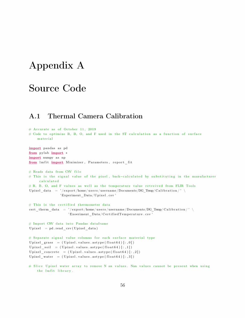
Appendix A

Source Code

A.1 Thermal Camera Calibration

# Accurate as o f October 11 , 2019# Code to opt imize R, B, O, and F used in the ST c a l c u l a t i o n as a func t i on o f s u r f a c e

mate r i a l

import pandas as pdfrom pylab import ∗import numpy as npfrom lm f i t import Minimizer , Parameters , r epo r t_ f i t

# Reads data from CSV f i l e# This i s the s i g n a l va lue o f the p ixe l , back−c a l c u l a t ed by sub s t i t u t i n g in the manufacturer

c a l c u l a t ed# R, B, O, and F va lues as we l l as the temperature va lue r e t r e i v e d from FLIR ToolsUpixel_data = ’ / export /home/ us e r s /username/Documents/DG_Temp/Ca l i b ra t i on / ’ \

’ Experiment_Data/Upixel . csv ’

# This i s the c e r t i f i e d thermometer datacert_therm_data = ’ / export /home/ use r s /username/Documents/DG_Temp/Ca l i b r a t i on / ’ \

’ Exoeriment_Data/Cert i f i edTemperature . csv ’

# Import CSV data in to Pandas dataframeUpixel = pd . read_csv ( Upixel_data )

# Separate s i g n a l va lue columns f o r each su r f a c e mate r i a l typeUpixel_grass = ( Upixel . va lue s . astype ( f l o a t 6 4 ) [ : , 0 ] )Up ixe l_so i l = ( Upixel . va lue s . astype ( f l o a t 6 4 ) [ : , 1 ] )Upixe l_concrete = ( Upixel . va lue s . astype ( f l o a t 6 4 ) [ : , 2 ] )Upixel_water = ( Upixel . va lue s . astype ( f l o a t 6 4 ) [ : , 3 ] )

# S l i c e Upixel water array to remove N an va lues . Nan va lue s cannot be pre sent when us ingthe lm f i t l i b r a r y .

56

# Water temperature data was not c o l l e c t e d f o r each time i n t e r va l , Nan va lues cannot be# present when us ing the lm f i t l i b r a r yUpixel_water = Upixel_water [ 0 : 7 ]

# Cal l in the c e r t i f i e d thermometer temperature datacert_therm = pd . read_csv ( cert_therm_data )

# Separate c e r t i f i e d temperature columns f o r each su r f a c e mate r i a l typecert_therm_grass = ( cert_therm . va lue s . astype ( f l o a t 6 4 ) [ : , 0 ] )cert_therm_soi l = ( cert_therm . va lue s . astype ( f l o a t 6 4 ) [ : , 1 ] )cert_therm_concrete = ( cert_therm . va lue s . astype ( f l o a t 6 4 ) [ : , 2 ] )cert_therm_water = ( cert_therm . va lue s . astype ( f l o a t 6 4 ) [ : , 3 ] )

# S l i c e thermometer water array . Nan va lues cannot be pre sent when us ing the lm f i t l i b r a r y .# Water temperature data was not c o l l e c t e d f o r each time i n t e r v a lcert_therm_water = cert_therm_water [ 0 : 7 ]

########################################################################################## Create ar rays f o r the s i g n a l va lue and c e r t i f i e d temperature f o r each land su r f a c e

mate r i a l .# Can on l t c a l i b r a t e one su r f a c e mate r i a l at a time .# For GrassUpixel_counts = np . array ( Upixel_grass , dtype=f l o a t 6 4 )cert_temp = np . array ( cert_therm_grass , dtype=f l o a t 6 4 )

# # For S o i l# Upixel_counts = np . array ( Upixe l_so i l , dtype=f l o a t 6 4 )# cert_temp = np . array ( cert_therm_soil , dtype=f l o a t 6 4 )

# # For Concrete# Upixel_counts = np . array ( Upixel_concrete , dtype=f l o a t 6 4 )# cert_temp = np . array ( cert_therm_concrete , dtype=f l o a t 6 4 )

# # For Water# Upixel_counts = np . array ( Upixel_water , dtype=f l o a t 6 4 )# cert_temp = np . array ( cert_therm_water , dtype=f l o a t 6 4 )########################################################################################### Def ine ob j e c t i v e funct ion , r e turn the array to be minimiseddef fcn2min ( params , Upixel_counts , cert_temp ) :

B = params [ ’B ’ ]R = params [ ’R ’ ]O = params [ ’O ’ ]F = params [ ’F ’ ]

model = B / np . l og (R / ( Upixel_counts + O) + F)

return model − cert_temp

# Create a s e t o f Parameters (R, B, O, and F) with the manufacturer va lue and maximum/minimum va lues

params = Parameters ( )

57

# Declare manufacturer constant va lue s and s e t maximum/minimum po s s i b l e constant va lue sparams . add ( ’B ’ , va lue=1428 , min=714 , max=2142)params . add ( ’R ’ , va lue =366545 , min=183272 , max=549817)params . add ( ’O’ , va lue=−342, min=−513, max=−171)params . add ( ’F ’ , va lue=1, min=0.5 , max=1.5)

# Use the l e a s t squares model and f i t the curve to the imported dataminner = Minimizer ( fcn2min , params , fcn_args=(Upixel_counts , cert_temp ) )r e s u l t = minner . minimize ( )

# Calcu la te the f i n a l r e s u l tf i n a l = cert_temp + r e s u l t . r e s i d u a l

# Print Fi t S t a t i s t i c s , Var i ab l e s (R, B, O, and F) and Cor r e l a t i on sr epo r t_ f i t ( r e s u l t )

# Try to p l o t the non l i n e a r f i ttry :

import matp lo t l i b . pyplot as p l t

p l t . p l o t ( Upixel_counts , cert_temp , ’ k+’ )p l t . p l o t ( Upixel_counts , f i n a l , ’ ro ’ )p l t . show ( )

except ImportError :pass

A.1.1 Thermal Camera Calibration Plots

import numpyfrom matp lo t l i b import pyplot as p l t

# F i l e with c e r t i f i e d temperaturec e r t i f i e d_t empe ra tu r e_ f i l e = ’ / export /home/ use r s /username/Documents/DG_Temp/ ’ \

’ Ca l i b ra t i on /Experiment_Data/Cert i f i edTemperature . csv ’

# F i l e with cor re spond ing Upixel ( raw s i g n a l ) va lue sUpixe l_va lues_f i l e = ’ / export /home/ use r s /username/Documents/ ’ \

’DG_Temp/Ca l i b ra t i on /Experiment_Data/Upixel . csv ’

# Import c e r t i f i e d temperature datacert i f i ed_temperature_data = numpy . genfromtxt ( c e r t i f i ed_tempe ra tu r e_ f i l e , d e l im i t e r=’ , ’ )

# Separate Columnscert_grass_temp = cert i f i ed_temperature_data [ : , 0 ]cert_soi l_temp = cert i f i ed_temperature_data [ : , 1 ]cert_concrete_temp = cert i f i ed_temperature_data [ : , 2 ]cert_water_temp = cert i f i ed_temperature_data [ : , 3 ]

########################################################################################################################

58

# Import image Upixel ( raw s i g n a l ) dataUpixel_values_data = numpy . genfromtxt ( Upixe l_va lues_f i l e , d e l im i t e r=’ , ’ )

# Separate ColumnsUpixel_values_grass = Upixel_values_data [ : , 0 ]Upixe l_values_so i l = Upixel_values_data [ : , 1 ]Upixel_values_concrete = Upixel_values_data [ : , 2 ]Upixel_values_water = Upixel_values_data [ : , 3 ]

# Remove Nan dataUpixel_values_water = Upixel_values_water [ 0 : 8 ]

# State o r i g i n a l FLIR f a c t o r y Planck constants , from image metadataR1_f l i r = 17096.453R2_f l i r = 0.046642166B_f l i r = 1428O_fl i r =−342F_f l i r =1

R_f l i r = R1_f l i r /R2_f l i r

# Back−c a l c u l a t e Temperature From Upixel va lue s# I n i t i a l i z e Arraysbackcalc_grass_temp = numpy . z e r o s ( ( len ( Upixel_values_grass ) ) )backcalc_soil_temp = numpy . z e r o s ( ( len ( Upixe l_values_so i l ) ) )backcalc_concrete_temp = numpy . z e r o s ( ( len ( Upixel_values_concrete ) ) )backcalc_water_temp = numpy . z e r o s ( ( len ( Upixel_values_water ) ) )

# Back−c a l c u l a t e image p i x e l temperature based on Upixel data and Factory s e t FLIR Constantsfor i in range (0 , len ( Upixel_values_grass ) ) :

backcalc_grass_temp [ i ] = B_f l i r /(numpy . l og ( R1_f l i r /( R2_f l i r ∗( Upixel_values_grass [ i ]+O_fl i r ) )+F_f l i r ) )

backcalc_soil_temp [ i ] = B_f l i r /(numpy . l og ( R1_f l i r /( R2_f l i r ∗( Upixe l_values_so i l [ i ]+O_fl i r) )+F_f l i r ) )

backcalc_concrete_temp [ i ] = B_f l i r /(numpy . l og ( R1_f l i r /( R2_f l i r ∗( Upixel_values_concrete [ i]+O_fl i r ) )+F_f l i r ) )

for i in range (0 , len ( backcalc_water_temp ) ) :backcalc_water_temp [ i ] = B_f l i r / (numpy . l og ( R1_f l i r / ( R2_f l i r ∗ ( Upixel_values_water [ i

] + O_fl i r ) ) + F_f l i r ) )

# Calcu la te Error , Square Error , Percentage Error , Bias , RMSE, and average percentage e r r o r# between c e r t i f i e d temperature and back−c a l c u l a t ed temperature# I n i t i a l i z e a r rays# Back−c a l c u l a t e Grassbackca lc_grass_error = numpy . z e r o s ( ( len ( Upixel_values_grass ) ) )backcalc_grass_sq_error = numpy . z e r o s ( ( len ( Upixel_values_grass ) ) )backcalc_grass_PE = numpy . z e r o s ( ( len ( Upixel_values_grass ) ) )

# Back−c a l c u l a t e S o i lbackca l c_so i l_er ro r = numpy . z e r o s ( ( len ( Upixe l_values_so i l ) ) )

59

backca lc_so i l_sq_error = numpy . z e r o s ( ( len ( Upixe l_values_so i l ) ) )backcalc_soil_PE = numpy . z e r o s ( ( len ( Upixe l_values_so i l ) ) )

# Back−c a l c u l a t e Concretebackca lc_concrete_error = numpy . z e r o s ( ( len ( Upixel_values_concrete ) ) )backcalc_concrete_sq_error = numpy . z e r o s ( ( len ( Upixel_values_concrete ) ) )backcalc_concrete_PE = numpy . z e r o s ( ( len ( Upixel_values_concrete ) ) )

# Back−c a l c u l a t e Waterbackcalc_water_error = numpy . z e r o s ( ( len ( Upixel_values_water ) ) )backcalc_water_sq_error = numpy . z e r o s ( ( len ( Upixel_values_water ) ) )backcalc_water_PE = numpy . z e r o s ( ( len ( Upixel_values_water ) ) )

# Calcu la te e r r o r in back−c a l c u l a t ed temperaturesfor i in range (0 , len ( Upixel_values_grass ) ) :

backca lc_grass_error [ i ] = backcalc_grass_temp [ i ]−cert_grass_temp [ i ]backca l c_so i l_er ro r [ i ] = backcalc_soil_temp [ i ]− cert_soi l_temp [ i ]backca lc_concrete_error [ i ] = backcalc_concrete_temp [ i ]−cert_concrete_temp [ i ]

for i in range (0 , len ( backcalc_water_temp ) ) :backcalc_water_error [ i ] = backcalc_water_temp [ i ]−cert_water_temp [ i ]

# Ca lcu la te Temperature Bias f o r each mate r i a lbackcalc_grass_bias = numpy . average ( backca lc_grass_error )backca l c_so i l_bias = numpy . average ( backca l c_so i l_er ro r )backcalc_concrete_bias = numpy . average ( backca lc_concrete_error )backcalc_water_bias = numpy . average ( backcalc_water_error )

# Calcu la te Square Errorfor i in range (0 , len ( Upixel_values_grass ) ) :

backcalc_grass_sq_error [ i ] = backca lc_grass_error [ i ]∗∗2backca lc_so i l_sq_error [ i ] = backca l c_so i l_er ro r [ i ]∗∗2backcalc_concrete_sq_error [ i ] = backca lc_concrete_error [ i ]∗∗2

for i in range (0 , len ( backcalc_water_temp ) ) :backcalc_water_sq_error [ i ] = backcalc_water_error [ i ]∗∗2

# Calcu la te RMSEbackcalc_grass_RMSE = numpy . sq r t (numpy . average ( backcalc_grass_sq_error ) )backcalc_soil_RMSE = numpy . sq r t (numpy . average ( backca lc_so i l_sq_error ) )backcalc_concrete_RMSE = numpy . sq r t (numpy . average ( backcalc_concrete_sq_error ) )backcalc_water_RMSE = numpy . sq r t (numpy . average ( backcalc_water_sq_error ) )

# Calcu la te Percentage Error (PE)for i in range (0 , len ( Upixel_values_grass ) ) :

backcalc_grass_PE [ i ] = numpy . abs ( ( cert_grass_temp [ i ]−backcalc_grass_temp [ i ] ) /cert_grass_temp [ i ] ) ∗100

backcalc_soil_PE [ i ] = numpy . abs ( ( cert_soi l_temp [ i ]−backcalc_soil_temp [ i ] ) / cert_soi l_temp[ i ] ) ∗100

backcalc_concrete_PE [ i ] = numpy . abs ( ( cert_concrete_temp [ i ]−backcalc_concrete_temp [ i ] ) /cert_concrete_temp [ i ] ) ∗100

60

for i in range (0 , len ( backcalc_water_temp ) ) :backcalc_water_PE [ i ] = numpy . abs ( ( cert_water_temp [ i ]−backcalc_water_temp [ i ] ) /

cert_water_temp [ i ] ) ∗100

# Calcu la te Average Percentage Errorbackcalc_grass_average_PE = numpy . average ( backcalc_grass_PE )backcalc_soil_average_PE = numpy . average ( backcalc_soil_PE )backcalc_concrete_average_PE = numpy . average ( backcalc_concrete_PE )backcalc_water_average_PE = numpy . average ( backcalc_water_PE )

########################################################################################################################

# LMFIT ( us ing the lm f i t l i b r a r y ) Planck Constants and Temperature back−c a l c u l a t e# GrassR_lmfit_grass = 314531B_lmfit_grass = 1391O_lmfit_grass = −513F_lmfit_grass = 1 .5

# So i lR_lmfit_soi l = 549800B_lmfit_soi l = 1510O_lmfit_soi l = −171F_lmfit_soi l = 1 .5

# ConcreteR_lmfit_concrete = 247614B_lmfit_concrete = 1322O_lmfit_concrete = −513F_lmfit_concrete = 1 .5

# WaterR_lmfit_water = 549789B_lmfit_water = 1507O_lmfit_water = −171F_lmfit_water = 1 .5

# Back−c a l c u l a t e temperature g iven new cons tant s and Upixel va lue s# I n i t i a l i z e a r rays# Grasslmfit_grass_temp = numpy . z e r o s ( ( len ( Upixel_values_grass ) ) )lmf i t_gras s_error = numpy . z e r o s ( ( len ( Upixel_values_grass ) ) )lmf i t_grass_sq_error = numpy . z e r o s ( ( len ( Upixel_values_grass ) ) )

# So i llmfit_soi l_temp = numpy . z e r o s ( ( len ( Upixe l_values_so i l ) ) )lm f i t_so i l_e r r o r = numpy . z e r o s ( ( len ( Upixe l_values_so i l ) ) )lmf i t_so i l_sq_error = numpy . z e r o s ( ( len ( Upixe l_values_so i l ) ) )

# Concretelmfit_concrete_temp = numpy . z e r o s ( ( len ( Upixel_values_concrete ) ) )

61

lmf i t_concre te_error = numpy . z e r o s ( ( len ( Upixel_values_concrete ) ) )lmf i t_concrete_sq_error = numpy . z e r o s ( ( len ( Upixel_values_concrete ) ) )

# Waterlmfit_water_temp = numpy . z e r o s ( ( len ( Upixel_values_water ) ) )lmf it_water_error = numpy . z e r o s ( ( len ( Upixel_values_water ) ) )lmfit_water_sq_error = numpy . z e r o s ( ( len ( Upixel_values_water ) ) )

# Back−c a l c u l a t e temperature ac co rd ing lyfor i in range (0 , len ( Upixel_values_grass ) ) :

lmfit_grass_temp [ i ] = B_lmfit_grass / (numpy . l og ( R_lmfit_grass / ( Upixel_values_grass [ i ]+ O_lmfit_grass ) + F_lmfit_grass ) )

lmfit_soi l_temp [ i ] = B_lmfit_soi l / (numpy . l og ( R_lmfit_soi l / ( Upixe l_values_so i l [ i ] +O_lmfit_soi l ) + F_lmfit_soi l ) )

lmfit_concrete_temp [ i ] = B_lmfit_concrete / (numpy . l og ( R_lmfit_concrete / (Upixel_values_concrete [ i ] + O_lmfit_concrete ) + F_lmfit_concrete ) )

for i in range (0 , len ( backcalc_water_temp ) ) :lmfit_water_temp [ i ] = B_lmfit_water / (numpy . l og ( R_lmfit_water / ( Upixel_values_water [ i ]

+ O_lmfit_water ) + F_lmfit_water ) )

# Calcu la te e r ro r , Square Error , b i a s and RMSE f o r back−c a l c u l a t ed LMFIT temperature# I n i t i a l i z e a r rays# LMFIT e r r o rfor i in range (0 , len ( Upixel_values_grass ) ) :

lmf i t_gras s_error [ i ] = lmfit_grass_temp [ i ] − cert_grass_temp [ i ]lm f i t_so i l_e r r o r [ i ] = lmfit_soi l_temp [ i ] − cert_soi l_temp [ i ]lmf i t_concre te_error [ i ] = lmfit_concrete_temp [ i ] − cert_concrete_temp [ i ]

for i in range (0 , len ( backcalc_water_temp ) ) :lmf it_water_error [ i ] = lmfit_water_temp [ i ] − cert_water_temp [ i ]

# Bias c a l c u l a t i o nlmf i t_grass_bias = numpy . average ( lmf i t_gras s_error )lm f i t_so i l_b ia s = numpy . average ( lm f i t_so i l_e r r o r )lmf i t_concrete_bias = numpy . average ( lmf i t_concre te_error )lmfit_water_bias = numpy . average ( lmf it_water_error )

# LMFIT square e r r o rfor i in range (0 , len ( Upixel_values_grass ) ) :

lmf i t_grass_sq_error [ i ] = lmf i t_gras s_error [ i ]∗∗2lmf i t_so i l_sq_error [ i ] = lm f i t_so i l_e r r o r [ i ]∗∗2lmf i t_concrete_sq_error [ i ] = lmf i t_concre te_error [ i ]∗∗2

for i in range (0 , len ( backcalc_water_temp ) ) :lmfit_water_sq_error [ i ] = lmfit_water_error [ i ]∗∗2

# Calcu la te RMSElmfit_grass_rmse = numpy . sq r t (numpy . average ( lmf it_grass_sq_error ) )lmf i t_so i l_rmse = numpy . sq r t (numpy . average ( lmf i t_so i l_sq_error ) )lmfit_concrete_rmse = numpy . sq r t (numpy . average ( lmf i t_concrete_sq_error ) )lmfit_water_rmse = numpy . sq r t (numpy . average ( lmfit_water_sq_error ) )

62

########################################################################################################################

# Plot Upixel vs c e r t i f i e d temperature f o r Grass , s o i l , concrete , and water c on s i d e r i ng thec a l i b r a t i o n

# experiment , the c a l i b r a t e d camera parameters , and the d e f au l t camera parametersf i g_d i r e c t = ’ / export /home/ us e r s /username/Documents/DG_Temp/ ’ \

’ Ca l i b ra t i on /Cal ibrated_Figures / ’# Grassp l t . f i g u r e ( )# Ca l i b r a t i on experimentp l t . s c a t t e r ( Upixel_values_grass , cert_grass_temp , c=’k ’ , marker=’+’ )# Defau l t Camera Parametersp l t . s c a t t e r ( Upixel_values_grass , backcalc_grass_temp , c=’ g ’ , marker=’d ’ )# Caibrated camera parametersp l t . s c a t t e r ( Upixel_values_grass , lmfit_grass_temp , c=’ r ’ , marker=’ ∗ ’ )p l t . x l ab e l ( ’ Uobject ␣ [A/D␣Counts ] ’ )p l t . y l ab e l ( ’ C e r t i f i e d ␣Temperature␣ [K] ’ )p l t . l egend ( [ ’ Ca l i b ra t i on ␣Experiment ’ , ’ De fau l t ␣Camera␣Parameters ’ , ’ Ca l ib rated ␣Camera␣

Parameters ’ ] )p l t . s a v e f i g ( f i g_d i r e c t+’ Gras sCa l ib ra t i on . png ’ )p l t . show ( )

# So i lp l t . f i g u r e ( )# Ca l i b r a t i on experimentp l t . s c a t t e r ( Upixe l_values_soi l , cert_soil_temp , c=’k ’ , marker=’+’ )# Defau l t Camera Parametersp l t . s c a t t e r ( Upixe l_values_soi l , backcalc_soil_temp , c=’ g ’ , marker=’d ’ )# Caibrated camera parametersp l t . s c a t t e r ( Upixe l_values_soi l , lmfit_soi l_temp , c=’ r ’ , marker=’ ∗ ’ )p l t . x l ab e l ( ’ Uobject ␣ [A/D␣Counts ] ’ )p l t . y l ab e l ( ’ C e r t i f i e d ␣Temperature␣ [K] ’ )p l t . l egend ( [ ’ Ca l i b ra t i on ␣Experiment ’ , ’ De fau l t ␣Camera␣Parameters ’ , ’ Ca l ib rated ␣Camera␣

Parameters ’ ] )p l t . s a v e f i g ( f i g_d i r e c t+’ S o i lCa l i b r a t i o n . png ’ )p l t . show ( )

# Concrete /Developed landp l t . f i g u r e ( )# Ca l i b r a t i on experimentp l t . s c a t t e r ( Upixel_values_concrete , cert_concrete_temp , c=’k ’ , marker=’+’ )# Defau l t Camera Parametersp l t . s c a t t e r ( Upixel_values_concrete , backcalc_concrete_temp , c=’ g ’ , marker=’d ’ )# Caibrated camera parametersp l t . s c a t t e r ( Upixel_values_concrete , lmfit_concrete_temp , c=’ r ’ , marker=’ ∗ ’ )p l t . x l ab e l ( ’ Uobject ␣ [A/D␣Counts ] ’ )p l t . y l ab e l ( ’ C e r t i f i e d ␣Temperature␣ [K] ’ )p l t . l egend ( [ ’ Ca l i b ra t i on ␣Experiment ’ , ’ De fau l t ␣Camera␣Parameters ’ , ’ Ca l ib rated ␣Camera␣

Parameters ’ ] )p l t . s a v e f i g ( f i g_d i r e c t+’ DevelopedLandCal ibrat ion . png ’ )

63

p l t . show ( )

# Remove Nan water datacert_water_temp = cert_water_temp [ 0 : 8 ]

# Waterp l t . f i g u r e ( )# Ca l i b r a t i on experimentp l t . s c a t t e r ( Upixel_values_water , cert_water_temp , c=’k ’ , marker=’+’ )# Defau l t Camera Parametersp l t . s c a t t e r ( Upixel_values_water , backcalc_water_temp , c=’ g ’ , marker=’d ’ )# Caibrated camera parametersp l t . s c a t t e r ( Upixel_values_water , lmfit_water_temp , c=’ r ’ , marker=’ ∗ ’ )p l t . x l ab e l ( ’ Uobject ␣ [A/D␣Counts ] ’ )p l t . y l ab e l ( ’ C e r t i f i e d ␣Temperature␣ [K] ’ )p l t . l egend ( [ ’ Ca l i b ra t i on ␣Experiment ’ , ’ De fau l t ␣Camera␣Parameters ’ , ’ Ca l ib rated ␣Camera␣

Parameters ’ ] )p l t . s a v e f i g ( f i g_d i r e c t+’WaterCal ibrat ion . png ’ )p l t . show ( )

A.2 Mining Site Campaign

A.2.1 TriSonica Atmospheric Pressure to Altitude

# Code to load in Tr i s on i ca data , concatenate data f o r e n t i r e May 2018 campaign , andc a l c u l a t e 1 second averaged data

# Current as o f October 16 , 2019import sysimport numpyimport datet imeimport matp lo t l i b . dates as datesfrom datet ime import date

# Cal l in Tr i s on i ca data f o r each day a f t e r complet ing pre l im inary# proc e s s i ng ( us ing ex c e l / l i b r e o f f i c e Calc to remove co lon / cha rac t e r# d e l im i t e r s and remove Nan data e tc . such that data can e a s i l y# be post proce s sed in Python )

# The TriSonica data has been pre−proces sed be f o r e being loaded in to t h i s s c r i p t . I nd i c e s o fascending and

# descending TANAB2 launches have been i d e n t i f e d from another s c r i p t and were used toc r e a t e a f i l e used in

# th i s s c r i p t i d e n t i f y i n g the ground l e v e l Pres sure ( A l t i tude ) at the s t a r t o f each TANAB2p r o f i l e

# May 7/2018# Cal l in a l l Pres sure Data in c l ud ing year , month , hour , minute , secondsfileName_MFT = ’ / export /home/ use r s /username/Documents/DG_Temp/Mining_Facil ity_2018/Tr iSonica

/Unaveraged/ ’ \’ Cleaned_Files / Ind iv idua l_F i l e s /2018−05−07−Data . txt ’

64

data_MFT = numpy . genfromtxt ( fileName_MFT , skip_header=5, i nva l i d_ra i s e=False ,u s e c o l s =(0 , 1 , 2 , 3 , 4 , 5 , 11 , 13) , miss ing_values=’ ’ ,

f i l l i n g_v a l u e s=numpy . nan )

# Separate columnsyear_MFT = data_MFT [ : , 0 ]month_MFT = data_MFT [ : , 1 ]day_MFT = data_MFT [ : , 2 ]hour_MFT = data_MFT [ : , 3 ]minute_MFT = data_MFT [ : , 4 ]seconds_MFT = data_MFT [ : , 5 ]temp_MFT = data_MFT [ : , 6 ]P_MFT = data_MFT [ : , 7 ]

# May 9/2018fileName_09_05_2018 = ’ / export /home/ use r s /username/Documents/DG_Temp/Mining_Facil ity_2018/

Tr iSonica /Unaveraged/ ’ \’ Cleaned_Files / Ind iv idua l_F i l e s /2018−05−09−Data . txt ’

data_09_05_2018 = numpy . genfromtxt ( fileName_09_05_2018 , skip_header=5, i n va l i d_ra i s e=False ,u s e c o l s =(0 , 1 , 2 , 3 , 4 , 5 , 11 , 13) , miss ing_values=’ ’ ,

f i l l i n g_v a l u e s=numpy . nan )

# Separate columnsyear_09_05_2018 = data_09_05_2018 [ : , 0 ]month_09_05_2018 = data_09_05_2018 [ : , 1 ]day_09_05_2018 = data_09_05_2018 [ : , 2 ]hour_09_05_2018 = data_09_05_2018 [ : , 3 ]minute_09_05_2018 = data_09_05_2018 [ : , 4 ]seconds_09_05_2018 = data_09_05_2018 [ : , 5 ]temp_09_05_2018 = data_09_05_2018 [ : , 6 ]P_09_05_2018 = data_09_05_2018 [ : , 7 ]

# May 10/2018fileName_10_05_2018 = ’ / export /home/ use r s /username/Documents/DG_Temp/Mining_Facil ity_2018/

Tr iSonica /Unaveraged/ ’ \’ Cleaned_Files / Ind iv idua l_F i l e s /2018−05−10−Data . txt ’

data_10_05_2018 = numpy . genfromtxt ( fileName_10_05_2018 , skip_header=5, i n va l i d_ra i s e=False ,u s e c o l s =(0 , 1 , 2 , 3 , 4 , 5 , 11 , 13) , miss ing_values=’ ’ ,

f i l l i n g_v a l u e s=numpy . nan )

# Separate columnsyear_10_05_2018 = data_10_05_2018 [ : , 0 ]month_10_05_2018 = data_10_05_2018 [ : , 1 ]day_10_05_2018 = data_10_05_2018 [ : , 2 ]hour_10_05_2018 = data_10_05_2018 [ : , 3 ]minute_10_05_2018 = data_10_05_2018 [ : , 4 ]seconds_10_05_2018 = data_10_05_2018 [ : , 5 ]temp_10_05_2018 = data_10_05_2018 [ : , 6 ]P_10_05_2018 = data_10_05_2018 [ : , 7 ]

65

# May 15/2018fileName_15_05_2018 = ’ / export /home/ use r s /username/Documents/DG_Temp/Mining_Facil ity_2018/

Tr iSonica /Unaveraged/ ’ \’ Cleaned_Files / Ind iv idua l_F i l e s /2018−05−15−Data . txt ’

data_15_05_2018 = numpy . genfromtxt ( fileName_15_05_2018 , skip_header=5, i n va l i d_ra i s e=False ,u s e c o l s =(0 , 1 , 2 , 3 , 4 , 5 , 11 , 13) , miss ing_values=’ ’ ,

f i l l i n g_v a l u e s=numpy . nan )

# Separate columnsyear_15_05_2018 = data_15_05_2018 [ : , 0 ]month_15_05_2018 = data_15_05_2018 [ : , 1 ]day_15_05_2018 = data_15_05_2018 [ : , 2 ]hour_15_05_2018 = data_15_05_2018 [ : , 3 ]minute_15_05_2018 = data_15_05_2018 [ : , 4 ]seconds_15_05_2018 = data_15_05_2018 [ : , 5 ]temp_15_05_2018 = data_15_05_2018 [ : , 6 ]P_15_05_2018 = data_15_05_2018 [ : , 7 ]

# May 18/2018fileName_18_05_2018 = ’ / export /home/ use r s /username/Documents/DG_Temp/Mining_Facil ity_2018/

Tr iSonica /Unaveraged/ ’ \’ Cleaned_Files / Ind iv idua l_F i l e s /2018−05−18−Data . txt ’

data_18_05_2018 = numpy . genfromtxt ( fileName_18_05_2018 , skip_header=5, i n va l i d_ra i s e=False ,u s e c o l s =(0 , 1 , 2 , 3 , 4 , 5 , 11 , 13) , miss ing_values=’ ’ ,

f i l l i n g_v a l u e s=numpy . nan )

# Separate columnsyear_18_05_2018 = data_18_05_2018 [ : , 0 ]month_18_05_2018 = data_18_05_2018 [ : , 1 ]day_18_05_2018 = data_18_05_2018 [ : , 2 ]hour_18_05_2018 = data_18_05_2018 [ : , 3 ]minute_18_05_2018 = data_18_05_2018 [ : , 4 ]seconds_18_05_2018 = data_18_05_2018 [ : , 5 ]temp_18_05_2018 = data_18_05_2018 [ : , 6 ]P_18_05_2018 = data_18_05_2018 [ : , 7 ]

# May 19/2018fileName_19_05_2018 = ’ / export /home/ use r s /username/Documents/DG_Temp/Mining_Facil ity_2018/

Tr iSonica /Unaveraged/ ’ \’ Cleaned_Files / Ind iv idua l_F i l e s /2018−05−19−Data . txt ’

data_19_05_2018 = numpy . genfromtxt ( fileName_19_05_2018 , skip_header=5, i n va l i d_ra i s e=False ,u s e c o l s =(0 , 1 , 2 , 3 , 4 , 5 , 11 , 13) , miss ing_values=’ ’ ,

f i l l i n g_v a l u e s=numpy . nan )

# Separate columnsyear_19_05_2018 = data_19_05_2018 [ : , 0 ]month_19_05_2018 = data_19_05_2018 [ : , 1 ]day_19_05_2018 = data_19_05_2018 [ : , 2 ]

66

hour_19_05_2018 = data_19_05_2018 [ : , 3 ]minute_19_05_2018 = data_19_05_2018 [ : , 4 ]seconds_19_05_2018 = data_19_05_2018 [ : , 5 ]temp_19_05_2018 = data_19_05_2018 [ : , 6 ]P_19_05_2018 = data_19_05_2018 [ : , 7 ]

# May 21/2018fileName_21_05_2018 = ’ / export /home/ use r s /username/Documents/DG_Temp/Mining_Facil ity_2018/

Tr iSonica /Unaveraged/ ’ \’ Cleaned_Files / Ind iv idua l_F i l e s /Tr iSonica/2018−05−21−Data . txt ’

data_21_05_2018 = numpy . genfromtxt ( fileName_21_05_2018 , skip_header=5, i n va l i d_ra i s e=False ,u s e c o l s =(0 , 1 , 2 , 3 , 4 , 5 , 11 , 13) , miss ing_values=’ ’ ,

f i l l i n g_v a l u e s=numpy . nan )

# Separate columnsyear_21_05_2018 = data_21_05_2018 [ : , 0 ]month_21_05_2018 = data_21_05_2018 [ : , 1 ]day_21_05_2018 = data_21_05_2018 [ : , 2 ]hour_21_05_2018 = data_21_05_2018 [ : , 3 ]minute_21_05_2018 = data_21_05_2018 [ : , 4 ]seconds_21_05_2018 = data_21_05_2018 [ : , 5 ]temp_21_05_2018 = data_21_05_2018 [ : , 6 ]P_21_05_2018 = data_21_05_2018 [ : , 7 ]

# May 23/2018fileName_23_05_2018 = ’ / export /home/ use r s /username/Documents/DG_Temp/Mining_Facil ity_2018/

Tr iSonica /Unaveraged/ ’ \’ Cleaned_Files / Ind iv idua l_F i l e s /2018−05−23−Data . txt ’

data_23_05_2018 = numpy . genfromtxt ( fileName_23_05_2018 , skip_header=5, i n va l i d_ra i s e=False ,u s e c o l s =(0 , 1 , 2 , 3 , 4 , 5 , 11 , 13) , miss ing_values=’ ’ ,

f i l l i n g_v a l u e s=numpy . nan )

# Separate columnsyear_23_05_2018 = data_23_05_2018 [ : , 0 ]month_23_05_2018 = data_23_05_2018 [ : , 1 ]day_23_05_2018 = data_23_05_2018 [ : , 2 ]hour_23_05_2018 = data_23_05_2018 [ : , 3 ]minute_23_05_2018 = data_23_05_2018 [ : , 4 ]seconds_23_05_2018 = data_23_05_2018 [ : , 5 ]temp_23_05_2018 = data_23_05_2018 [ : , 6 ]P_23_05_2018 = data_23_05_2018 [ : , 7 ]

# May 24/2018fileName_24_05_2018 = ’ / export /home/ use r s /username/Documents/DG_Temp/Mining_Facil ity_2018/

Tr iSonica /Unaveraged/ ’ \’ Cleaned_Files / Ind iv idua l_F i l e s /2018−05−24−Data . txt ’

data_24_05_2018 = numpy . genfromtxt ( fileName_24_05_2018 , skip_header=5, i n va l i d_ra i s e=False ,u s e c o l s =(0 , 1 , 2 , 3 , 4 , 5 , 11 , 13) , miss ing_values=’ ’ ,

f i l l i n g_v a l u e s=numpy . nan )

67

# Separate columnsyear_24_05_2018 = data_24_05_2018 [ : , 0 ]month_24_05_2018 = data_24_05_2018 [ : , 1 ]day_24_05_2018 = data_24_05_2018 [ : , 2 ]hour_24_05_2018 = data_24_05_2018 [ : , 3 ]minute_24_05_2018 = data_24_05_2018 [ : , 4 ]seconds_24_05_2018 = data_24_05_2018 [ : , 5 ]temp_24_05_2018 = data_24_05_2018 [ : , 6 ]P_24_05_2018 = data_24_05_2018 [ : , 7 ]

# May 27/2018fileName_27_05_2018 = ’ / export /home/ use r s /username/Documents/DG_Temp/Mining_Facil ity_2018/

Tr iSonica /Unaveraged/ ’ \’ Cleaned_Files / Ind iv idua l_F i l e s /Tr iSonica/2018−05−27−Data . txt ’

data_27_05_2018 = numpy . genfromtxt ( fileName_27_05_2018 , skip_header=5, i n va l i d_ra i s e=False ,u s e c o l s =(0 , 1 , 2 , 3 , 4 , 5 , 11 , 13) , miss ing_values=’ ’ ,

f i l l i n g_v a l u e s=numpy . nan )

# Separate columnsyear_27_05_2018 = data_27_05_2018 [ : , 0 ]month_27_05_2018 = data_27_05_2018 [ : , 1 ]day_27_05_2018 = data_27_05_2018 [ : , 2 ]hour_27_05_2018 = data_27_05_2018 [ : , 3 ]minute_27_05_2018 = data_27_05_2018 [ : , 4 ]seconds_27_05_2018 = data_27_05_2018 [ : , 5 ]temp_27_05_2018 = data_27_05_2018 [ : , 6 ]P_27_05_2018 = data_27_05_2018 [ : , 7 ]

# May 30/2018fileName_30_05_2018 = ’ / export /home/ use r s /username/Documents/DG_Temp/Mining_Facil ity_2018/

Tr iSonica /Unaveraged/ ’ \’ Cleaned_Files / Ind iv idua l_F i l e s /2018−05−30−Data . txt ’

data_30_05_2018 = numpy . genfromtxt ( fileName_30_05_2018 , skip_header=5, i n va l i d_ra i s e=False ,u s e c o l s =(0 , 1 , 2 , 3 , 4 , 5 , 11 , 13) , miss ing_values=’ ’ ,

f i l l i n g_v a l u e s=numpy . nan )

# Separate columnsyear_30_05_2018 = data_30_05_2018 [ : , 0 ]month_30_05_2018 = data_30_05_2018 [ : , 1 ]day_30_05_2018 = data_30_05_2018 [ : , 2 ]hour_30_05_2018 = data_30_05_2018 [ : , 3 ]minute_30_05_2018 = data_30_05_2018 [ : , 4 ]seconds_30_05_2018 = data_30_05_2018 [ : , 5 ]temp_30_05_2018 = data_30_05_2018 [ : , 6 ]P_30_05_2018 = data_30_05_2018 [ : , 7 ]

# May 31/2018fileName_31_05_2018 = ’ / export /home/ use r s /username/Documents/DG_Temp/Mining_Facil ity_2018/

Tr iSonica /Unaveraged/ ’ \

68

’ Cleaned_Files / Ind iv idua l_F i l e s /2018−05−31−Data . txt ’

data_31_05_2018 = numpy . genfromtxt ( fileName_31_05_2018 , skip_header=5, i n va l i d_ra i s e=False ,u s e c o l s =(0 , 1 , 2 , 3 , 4 , 5 , 11 , 13) , miss ing_values=’ ’ ,

f i l l i n g_v a l u e s=numpy . nan )

# Separate columnsyear_31_05_2018 = data_31_05_2018 [ : , 0 ]month_31_05_2018 = data_31_05_2018 [ : , 1 ]day_31_05_2018 = data_31_05_2018 [ : , 2 ]hour_31_05_2018 = data_31_05_2018 [ : , 3 ]minute_31_05_2018 = data_31_05_2018 [ : , 4 ]seconds_31_05_2018 = data_31_05_2018 [ : , 5 ]temp_31_05_2018 = data_31_05_2018 [ : , 6 ]P_31_05_2018 = data_31_05_2018 [ : , 7 ]

# Concatenate columns toge the ryear = numpy . concatenate ( [ year_MFT, year_09_05_2018 , year_10_05_2018 , year_15_05_2018 ,

year_18_05_2018 ,year_19_05_2018 , year_21_05_2018 , year_23_05_2018 , year_24_05_2018

,year_27_05_2018 , year_30_05_2018 , year_31_05_2018 ] )

month = numpy . concatenate ( [month_MFT, month_09_05_2018 , month_10_05_2018 , month_15_05_2018 ,month_18_05_2018 ,

month_19_05_2018 , month_21_05_2018 , month_23_05_2018 ,month_24_05_2018 ,

month_27_05_2018 , month_30_05_2018 , month_31_05_2018 ] )day = numpy . concatenate ( [day_MFT, day_09_05_2018 , day_10_05_2018 , day_15_05_2018 ,

day_18_05_2018 ,day_19_05_2018 , day_21_05_2018 , day_23_05_2018 , day_24_05_2018 ,

day_27_05_2018 ,day_30_05_2018 , day_31_05_2018 ] )

hour = numpy . concatenate ( [ hour_MFT, hour_09_05_2018 , hour_10_05_2018 , hour_15_05_2018 ,hour_18_05_2018 ,

hour_19_05_2018 , hour_21_05_2018 , hour_23_05_2018 , hour_24_05_2018, hour_27_05_2018 ,

hour_30_05_2018 , hour_31_05_2018 ] )minute = numpy . concatenate ( [minute_MFT, minute_09_05_2018 , minute_10_05_2018 ,

minute_15_05_2018 ,minute_18_05_2018 , minute_19_05_2018 , minute_21_05_2018 ,

minute_23_05_2018 ,minute_24_05_2018 , minute_27_05_2018 , minute_30_05_2018 ,

minute_31_05_2018 ] )seconds = numpy . concatenate ( [ seconds_MFT , seconds_09_05_2018 , seconds_10_05_2018 ,

seconds_15_05_2018 ,seconds_18_05_2018 , seconds_19_05_2018 , seconds_21_05_2018 ,

seconds_23_05_2018 ,seconds_24_05_2018 , seconds_27_05_2018 , seconds_30_05_2018 ,

seconds_31_05_2018 ] )temp = numpy . concatenate ( ( [ temp_MFT, temp_09_05_2018 , temp_10_05_2018 , temp_15_05_2018 ,

temp_18_05_2018 ,temp_19_05_2018 , temp_21_05_2018 , temp_23_05_2018 ,

69

temp_24_05_2018 , temp_27_05_2018 ,temp_30_05_2018 , temp_31_05_2018 ] ) )

P = numpy . concatenate ( [P_MFT, P_09_05_2018 , P_10_05_2018 , P_15_05_2018 , P_18_05_2018 ,P_19_05_2018 , P_21_05_2018 ,

P_23_05_2018 , P_24_05_2018 , P_27_05_2018 , P_30_05_2018 , P_31_05_2018] )

# Calcu la te A l t i tude s from pre s su r e# From another an a l y s i s ( v ia f i r s t order f i t o f hypsometr ic equat ion ) d e f i n e 1 s t# order p o l y f i t c o e f f i c i e n t s to convert p r e s su r e to a l t i t u d e a l t=a∗p+ba = −8.51514286 e+00b = 8.62680905 e+03

# I n i t i a l i z e a l t i t u d e arraya l t i t u d e = numpy . z e r o s ( len ( year ) )print (P)

# Calcu la te a l t i t u d e f o r each indexfor i in range (0 , len ( a l t i t u d e ) ) :

a l t i t u d e [ i ] =(a∗P[ i ] )+b

# Calcu la te the number o f minutes passed s i n c e the beg inning o f 2018 ( based on day o f year )doy_min = numpy . z e r o s ( len ( year ) )for i in range (0 , len ( year ) ) :

i f day [ i ] == 7 :doy_min [ i ] = (127∗24∗60)+(hour [ i ]∗60 )+minute [ i ]

e l i f day [ i ] == 8 :doy_min [ i ] = (128∗24∗60)+(hour [ i ]∗60 )+minute [ i ]

e l i f day [ i ] == 9 :doy_min [ i ] = (129∗24∗60)+(hour [ i ]∗60 )+minute [ i ]

e l i f day [ i ] == 10 :doy_min [ i ] = (130∗24∗60)+(hour [ i ]∗60 )+minute [ i ]

e l i f day [ i ] == 15 :doy_min [ i ] = (135∗24∗60)+(hour [ i ]∗60 )+minute [ i ]

e l i f day [ i ] == 18 :doy_min [ i ] = (138∗24∗60)+(hour [ i ]∗60 )+minute [ i ]

e l i f day [ i ] == 19 :doy_min [ i ] = (139∗24∗60)+(hour [ i ]∗60 )+minute [ i ]

e l i f day [ i ] == 21 :doy_min [ i ] = (141∗24∗60)+(hour [ i ]∗60 )+minute [ i ]

e l i f day [ i ] == 23 :doy_min [ i ] = (143∗24∗60)+(hour [ i ]∗60 )+minute [ i ]

e l i f day [ i ] == 24 :

70

doy_min [ i ] = (144∗24∗60)+(hour [ i ]∗60 )+minute [ i ]

e l i f day [ i ] == 27 :doy_min [ i ] = (147∗24∗60)+(hour [ i ]∗60 )+minute [ i ]

e l i f day [ i ] == 30 :doy_min [ i ] = (150∗24∗60)+(hour [ i ]∗60 )+minute [ i ]

e l i f day [ i ] == 31 :doy_min [ i ] = (151∗24∗60)+(hour [ i ]∗60 )+minute [ i ]

else :print ( ’More␣Dates␣need␣ to ␣be␣ inc luded ␣above ’ )

# Save Unaveraged concatenated v a r i a b l e s and a l t i t u d e s to f i l etoday_date = datet ime . date . today ( ) . s t r f t im e ( "%B_%d_%Y" )

outputFileName = ’ / export /home/ us e r s /username/Documents/DG_Temp/Mining_Facil ity_2018/Tr iSonica /Unaveraged/ ’ \

’ Cleaned_Files /TriSonica_May_2018_Unaveraged_Airborne_Altitudes . txt ’outputF i l e = open( outputFileName , ’w ’ )outputF i l e . wr i t e ( "#␣Data␣ c o l l e c t e d ␣by␣Tr iSonica ␣ f o r ␣May␣2018␣ f i e l d ␣campaign . ␣ Inc lude s ␣

Al t i tude ␣ c a l c u l a t i o n ␣\n" )outputF i l e . wr i t e ( "#By : ␣Ryan␣Byerlay ␣\n" )outputF i l e . wr i t e ( "#Created␣on␣"+today_date+"␣\n" )outputF i l e . wr i t e ( "#Recorded␣Time␣ i s ␣Local ␣Time␣ (MDT)␣\n" )outputF i l e . wr i t e ( "#0:Year␣\ t ␣#1:Month␣\ t ␣#2:Day␣\ t ␣#3:Hour␣\ t ␣#4:Minute␣\ t ␣#5:Seconds␣\ t "

"␣#6:DOY␣In␣Minutes␣\ t ␣␣#7: Pressure ␣\ t ␣#8:Al t i tude ␣\n" )for i in range (0 , len ( year ) ) :

outputF i l e . wr i t e ( "%i ␣\ t ␣%i ␣\ t ␣%i ␣\ t ␣%i ␣\ t ␣%i ␣\ t ␣%f ""␣\ t ␣%f ␣\ t ␣%f ␣\ t ␣%f ␣\ t ␣%f ␣\n" % ( year [ i ] , month [ i ] , day [ i ] , hour [ i ] ,

minute [ i ] ,seconds [ i ] , doy_min [ i ] , P [ i ] , a l t i t u d e

[ i ] , temp [ i ] ) )outputF i l e . c l o s e ( )

########################################################################################################################

# Complete 1 second averag ing# Second Averaging (10 Hz Frequency )AverageSample = 10

# Total number o f samplesNtota l = numpy . s i z e ( a l t i t u d e )NSample = int ( Ntota l /AverageSample )

# Calcu la te 1 second averaged a l t i t ud e s , year , month , day , hour , minute , second ,# pressure , day o f year in minutes , and temperature averages f o r each sampleyearavg = numpy . z e r o s ( ( NSample , 1) )

71

monthavg = numpy . z e r o s ( ( NSample , 1) )houravg = numpy . z e r o s ( ( NSample , 1) )dayavg = numpy . z e r o s ( ( NSample , 1) )minuteavg = numpy . z e r o s ( ( NSample , 1) )secondavg = numpy . z e r o s ( ( NSample , 1) )pre s sureavg = numpy . z e r o s ( ( NSample , 1) )a l t i t udeavg = numpy . z e r o s ( ( NSample , 1) )doy_min_avg = numpy . z e r o s ( ( NSample , 1) )temp_avg = numpy . z e r o s ( ( NSample , 1) )

# Calcu la te Averagesfor i in range (0 , NSample ) :

yearavg [ i ] = numpy .mean( year [ i ∗AverageSample : ( i +1)∗AverageSample ] )monthavg [ i ] = numpy .mean(month [ i ∗AverageSample : ( i +1)∗AverageSample ] )houravg [ i ] = numpy .mean( hour [ i ∗AverageSample : ( i +1)∗AverageSample ] )dayavg [ i ] = numpy .mean( day [ i ∗AverageSample : ( i +1)∗AverageSample ] )minuteavg [ i ] = numpy .mean(minute [ i ∗AverageSample : ( i +1)∗AverageSample ] )secondavg [ i ] = numpy .mean( seconds [ i ∗AverageSample : ( i +1)∗AverageSample ] )pre s sureavg [ i ] = numpy .mean(P[ i ∗AverageSample : ( i +1)∗AverageSample ] )a l t i t udeavg [ i ] = numpy .mean( a l t i t u d e [ i ∗AverageSample : ( i +1)∗AverageSample ] )doy_min_avg [ i ] = numpy .mean(doy_min [ i ∗AverageSample : ( i +1)∗AverageSample ] )temp_avg [ i ] = numpy .mean( temp [ i ∗AverageSample : ( i +1)∗AverageSample ] )

# The f o l l ow i ng i s to the f i x the i s s u e where in the averaged second column ,# the 59 th averaged second does not equal 59 , i n s t ead i t i s a lower value . For example :# 58 , 59 , 0 are being averaged toge the r so the value w i l l be < 59# Inc lude a cond i t i on to omit Nan va lue s too# When saving , put in a check to see i f the va lue s are Nan , i f index has Nan values , then

sk ip indexfor i in range (0 , len ( secondavg ) ) :

print ( secondavg [ i ] )i f numpy . i snan ( secondavg [ i ] ) == True :

continue

else :print ( type ( secondavg [ i ] ) )print ( int ( secondavg [ i ] ) )i f int ( secondavg [ i ] ) == 58 and int ( secondavg [ i +1]) != 59 :

yearavg [ i +1] = numpy . nanmonthavg [ i +1] = numpy . nanhouravg [ i +1] = numpy . nandayavg [ i +1] = numpy . nanminuteavg [ i +1] = numpy . nansecondavg [ i +1] = numpy . nanpres sureavg [ i +1] = numpy . nana l t i t udeavg [ i +1] = numpy . nandoy_min_avg [ i +1] = numpy . nantemp_avg [ i +1] = numpy . nan

# Cal l in Tr iSonica Base Al t i tude f i l e s : Prev ious ly c rea ted from the i n d i c e s f i l e s f o r# each TANAB2 launch . The i n d i c e s f i l e i d e n t i f i e s the time and l o c a t i o n o f each TANAB2

launch .

72

f i leName_BaseAlt = ’ / export /home/ use r s /username/Documents/DG_Temp/Mining_Facil ity_2018/Tr iSonica /Unaveraged/ ’ \

’ Cleaned_Files /Ascending_Descending_TANAB2/BaseAltitudesTriSonica_V3 . txt ’

data_BaseAlt = numpy . genfromtxt ( fileName_BaseAlt , skip_header=5)

day_BaseAlt = data_BaseAlt [ : , 2 ]hour_BaseAlt = data_BaseAlt [ : , 3 ]minute_BaseAlt = data_BaseAlt [ : , 4 ]doy_BaseAlt = data_BaseAlt [ : , 6 ]BasePres sure_tr i son i ca = data_BaseAlt [ : , 7 ]BaseAl t_tr i son ica = data_BaseAlt [ : , 8 ]Location_BaseAlt = data_BaseAlt [ : , 9 ]

# I n i t i a l i z e v a r i a b l e that s t o r e s the d i f f e r e n c e between day o f year in minutes# f o r the Tr iSonica base a l t i t u d e and f o r the second averaged f i l edelta_doy = numpy . z e r o s ( ( len ( data_BaseAlt ) , 1 ) )

# I n i t i a l i z e BaseAlt i tude used to c a l c u l a t e change in a l t i t u d e and index_Base to# ind i c a t e the index with the sma l l e s t day o f year in minutes d i f f e r e n c eBaseAlt i tude = numpy . z e r o s ( ( NSample , 1 ) )BasePressure = numpy . z e r o s ( ( NSample , 1 ) )Locat ion = numpy . empty (NSample , dtype=str )index_Base = numpy . z e r o s ( ( NSample , 1 ) )

# Match day o f year in minutes i n d i c e s from Base Al t i tude f i l e & second averaged f i l e# loop through averaged day o f year in minutes i n d i c e sfor i in range (0 , len ( yearavg ) ) :

# Skip Nan va luesi f numpy . i snan ( yearavg [ i ] ) == True :

continueelse :

# Loop through Base Al t i tude i n d i c e sfor j in range (0 , len ( day_BaseAlt ) ) :

# Ca lcu la te d i f f e r e n c e between day o f year in minutes t imesdelta_doy [ j ] = abs ( doy_BaseAlt [ j ]−doy_min_avg [ i ] )

# When at the l a s t va lue o f the Base Al t i tude f i l e , f i nd the index with theminimum value

# Also record l o c a t i o n and index o f the Base Al t i tude f i l ei f j == ( len ( BaseAl t_tr i son ica )−1) :

BaseAlt i tude [ i ] = BaseAlt_tr i son ica [ numpy . argmin ( delta_doy ) ]BasePressure [ i ] = BasePres sure_tr i son i ca [ numpy . argmin ( delta_doy ) ]index_Base [ i ] = numpy . argmin ( delta_doy [ j ] )

# I n i t i a l i z e v a r i a b l e s f o r change in atmospher ic p r e s su r e and change in a l t i t u d e r e l a t i v e tothe ground

de l t aPr e s su r e = numpy . z e r o s ( ( NSample , 1 ) )d e l t aA l t i t ud e = numpy . z e r o s ( ( NSample , 1 ) )

# Calcu la te the change in p r e s su r e and the change in a l t i t u d e and a s s i gn geographicl o c a t i o n s to each index

73

for i in range (0 , NSample ) :# Skip Nan va luesi f numpy . i snan ( pres sureavg [ i ] ) == True :

continueelse :

d e l t aPr e s su r e [ i ] = abs ( BasePressure [ i ]−pres sureavg [ i ] )d e l t aA l t i t ud e [ i ] = abs ( BaseAlt i tude [ i ]− a l t i t udeavg [ i ] )

i f dayavg [ i ] == 7 or dayavg [ i ] == 8 :Locat ion [ i ] = ’T ’

e l i f dayavg [ i ] == 9 or dayavg [ i ] == 10 or dayavg [ i ] == 15 or dayavg [ i ] == 30 or dayavg [ i] == 31 :Locat ion [ i ] = ’B ’

e l i f dayavg [ i ] == 18 or dayavg [ i ] == 19 or dayavg [ i ] == 21 or dayavg [ i ] == 23 or dayavg [i ] == 24 or dayavg [ i ] == 27 :Locat ion [ i ] = ’M’

else :# Note : Need to manually remove rows with ’N ’ in the r e s u l t i n g text f i l eLocat ion [ i ] = ’N ’print ( ’Day␣ f a l l s ␣ ou t s id e ␣ o f ␣ the ␣ ones ␣ l i s t e d ␣above ’ )

print ( BaseAlt i tude )

# Save Averaged data to f i l eoutputFileName_avg = ’ / export /home/ use r s /username/Documents/DG_Temp/Mining_Facil ity_2018/

Tr iSonica / ’ \’ TriSonica_May2018_Altitudes_averaged . txt ’

outputFile_avg = open( outputFileName_avg , ’w ’ )outputFile_avg . wr i t e ( "#␣Second␣Avgeraged␣Data␣ c o l l e c t e d ␣by␣Tr iSonica ␣ f o r ␣May"

"␣2018␣ f i e l d ␣campiagn . ␣ Inc lude s ␣Al t i tude ␣ c a l c u l a t i o n ␣\n" )outputFile_avg . wr i t e ( "#By : ␣Ryan␣Byerlay ␣\n" )outputFile_avg . wr i t e ( "#Created␣on␣"+today_date+"␣\n" )outputFile_avg . wr i t e ( "#Recorded␣Time␣ i s ␣Local ␣Time␣ (MDT)␣\n" )outputFile_avg . wr i t e ( "#0:AvgYear␣\ t ␣#1:AvgMonth␣\ t ␣#2:AvgDay␣\ t "

"␣#3:AvgHour␣\ t ␣#4:AvgMinute␣\ t ␣#5:AvgSeconds␣\ t ␣#6: Locat ion ␣ (T=MFT/B=Berm/M=Mine/N=NoMatch) "

"␣\ t ␣#7:Day␣ o f ␣Year␣ in ␣minutes ␣\ t ␣#8:AvgPressure ␣\ t ␣#9:BasePressure ␣\ t ""␣#10: De l taPres sure ␣\ t ␣#11:AvgAltitude ␣\ t ␣#12: BaseAlt i tude ␣\ t ␣#13:

De l taAl t i tude ␣\ t ""␣#14:Temperature (degC) ␣\ t ␣#15: Index␣ in ␣BaseAlt ␣ F i l e ␣\n" )

for i in range (0 , NSample ) :# I f index has Nan value , sk ip and do not wr i t ei f numpy . i snan ( yearavg [ i ] ) == True :

continueelse :

outputFile_avg . wr i t e ( "%i ␣\ t ␣%i ␣\ t ␣%i ␣\ t ␣%i ␣\ t ␣%i ""␣\ t ␣%i ␣\ t ␣%s␣\ t ␣%f ␣\ t ␣%f ␣\ t ␣%f ""␣\ t ␣%f ␣\ t ␣%f ␣\ t ␣%f ␣\ t ␣%f ␣\ t ␣%f ""␣\ t ␣%i ␣\n" % ( yearavg [ i ] , monthavg [ i ] , dayavg [ i ] , houravg [ i ] ,

minuteavg [ i ] ,secondavg [ i ] , Locat ion [ i ] , doy_min_avg [ i ] ,

74

pres sureavg [ i ] , BasePressure [ i ] ,d e l t aPr e s su r e [ i ] , a l t i t udeavg [ i ] , BaseAlt i tude [ i

] , d e l t aA l t i t ude [ i ] ,temp_avg [ i ] , index_Base [ i ] ) )

outputFile_avg . c l o s e ( )

A.2.2 Spatial Coordinate Grid Overlaid on Mine Site

import numpyimport mathfrom math import rad iansfrom math import degree sfrom math import a s infrom math import tanfrom math import atan2from math import s i nfrom math import cosfrom math import acosfrom math import s q r tfrom math import atan

# Current as o f October 16 , 2019# Given a de s i r ed s p a t i a l r e s o l u t i on , c oo rd ina t e s about an approximately# 40km by 30km re c t ang l e around mine are c a l c u l a t ed and saved to a f i l e

# The crea ted f i l e can be imported in to QGIS and the coo rd ina t e s can be l a i d on top o fs a t e l l i t e images / r a s t e r

# f i l e s (MODIS emi s s i v i t y , s u r f a c e temperature and su r f a c e e l e v a t i o n e tc . ) and data from# the images can be ext rac t ed f o r each po int

# Calcu la te l a t i t u d e / l ong i tude coo rd ina t e s based on the de f ined s p a t i a l r e s o l u t i o ndef S i t eCoord inate sCa l c ( res_x , y_iterator , TLeft_lat_rads , R, TLeft_lon_rads , GPS_matrix ) :

for a in range (0 , res_x ) :for b in range (0 , res_y ) :

i f a == 0 and b == 0 :continue

e l i f a == 0 and b != 0 :d_km = y_ite ra to r [ b−1]Yaw = 180Yaw_rads = math . rad ians (Yaw)

l a t 2 = math . a s in (math . s i n ( TLeft_lat_rads ) ∗ math . cos (d_km / R) + math . cos (TLeft_lat_rads )

∗ math . s i n (d_km / R) ∗ math . cos (Yaw_rads ) )lon2 = TLeft_lon_rads + math . atan2 (math . s i n (Yaw_rads ) ∗ math . s i n (d_km / R) ∗

math . cos ( TLeft_lat_rads ) ,math . cos (d_km / R) − math . s i n (

TLeft_lat_rads ) ∗ math . s i n ( l a t 2 ) )

# Convert back to decimal degree sl a t 2 = math . degree s ( l a t 2 )

75

lon2 = math . degree s ( lon2 )

# Save to GPS MatrixGPS_matrix [ a ] [ b ] [ 0 ] = l a t 2GPS_matrix [ a ] [ b ] [ 1 ] = lon2continue

e l i f b == 0 and a != 0 :d_km = x_ite ra to r [ a−1]Yaw = 90Yaw_rads = math . rad ians (Yaw)

l a t 2 = math . a s in (math . s i n ( TLeft_lat_rads ) ∗ math . cos (d_km / R) + math . cos (TLeft_lat_rads )

∗ math . s i n (d_km / R) ∗ math . cos (Yaw_rads ) )lon2 = TLeft_lon_rads + math . atan2 (math . s i n (Yaw_rads ) ∗ math . s i n (d_km / R) ∗

math . cos ( TLeft_lat_rads ) ,math . cos (d_km / R) − math . s i n (

TLeft_lat_rads ) ∗ math . s i n ( l a t 2 ) )

# Convert back to decimal degree sl a t 2 = math . degree s ( l a t 2 )lon2 = math . degree s ( lon2 )

# Save to GPS MatrixGPS_matrix [ a ] [ b ] [ 0 ] = l a t 2GPS_matrix [ a ] [ b ] [ 1 ] = lon2continue

else :d_km = y_ite ra to r [ b ]Yaw = 180Yaw_rads = math . rad ians (Yaw)

l a t 2 = math . a s in (math . s i n (math . rad ians (GPS_matrix [ a ] [ 0 ] [ 0 ] ) ) ∗math . cos (d_km /R)

+ math . cos (math . rad ians (GPS_matrix [ a ] [ 0 ] [ 0 ] ) ) ∗ math . s i n (d_km/R) ∗math . cos (Yaw_rads ) )

lon2 = math . rad ians (GPS_matrix [ a ] [ 0 ] [ 1 ] ) + \math . atan2 (math . s i n (Yaw_rads ) ∗math . s i n (d_km/R) ∗ math . cos (math .

rad ians (GPS_matrix [ a ] [ 0 ] [ 0 ] ) ) ,math . cos (d_km/R)−math . s i n (math . rad ians (GPS_matrix [ a

] [ 0 ] [ 0 ] ) ) ∗math . s i n ( l a t 2 ) )

# Convert back to decimal degree sl a t 2 = math . degree s ( l a t 2 )lon2 = math . degree s ( lon2 )

# Save to GPS MatrixGPS_matrix [ a ] [ b ] [ 0 ] = l a t 2GPS_matrix [ a ] [ b ] [ 1 ] = lon2

76

return GPS_matrix

# Get GPS coo rd ina t e s f o r an approximately 40km by 30km re c t ang l e around mine# Id en t i f y the Top Le f t l a t i t u d e / l ong i tude# For the ho r i z on t a l loop# Use the top l e f t as a r e f e r e n c e po intTLeft_lat = XX.XXXXXXTLeft_lon = −XXX.XXXXXX

# Convert degree s to rad iansTLeft_lat_rads = rad ians ( TLeft_lat )TLeft_lon_rads = rad ians ( TLeft_lon )

# Ending l a t / lonTRight_lat = XX.XXXXXXTRight_lon = −XXX.XXXXX

# For the v e r t i c a l loop# Sta r t i ng l a t i t u d e / l ong i tudeBRight_lat = XX.XXXXXXBRight_lon = −XXX.XXXXXX

# Ending l a t i t u d e / l ong i tudeBLeft_lat = XX.XXXXXXBLeft_lon = −XXX.XXXXXX

# Equator ia l r ad iu s o f earth as per : https : // nssdc . g s f c . nasa . gov/ p lanetary / f a c t s h e e t /e a r t h f a c t . html

R = 6378.1

########################################################################################################################

# Number o f ho r i z on t a l and v e r t i c a l squares per s p a t i a l r e s o l u t i o n# 500m by 500m r e s o l u t i o nres500_x = 113res500_y = 114

# 100m by 100m r e s o l u t i o nres100_x = 570res100_y = 570

# 1km by 1km r e s o l u t i o nres1000_x = 57res1000_y = 57

########################################################################################################################

# For code below use the f o l l ow i n g r e s o l u t i o nres_x = res100_x

77

res_y = res100_y

# Create array f o r d e c l a r i n g the i t e r a t o r to be used f o r the ho r i z on t a l and v e r t i c a ld i r e c t i o n s

x_i te ra to r = numpy . z e r o s ( ( res_x , 1 ) )y_i te ra to r = numpy . z e r o s ( ( res_y , 1 ) )

# I n i t i a l i z e l ong i tude / l a t i t u d e matrixGPS_matrix = numpy . z e r o s ( ( res_x , res_y , 2) )

# Assign Known GPS l a t i t u d e / l ong i tude to matrixGPS_matrix [ 0 ] [ 0 ] [ 0 ] = TLeft_latGPS_matrix [ 0 ] [ 0 ] [ 1 ] = TLeft_lon

# The number o f GPS coo rd ina t e s to save to f i l elen_save = res_x∗ res_ysave_GPS_matrix = numpy . z e r o s ( ( len_save , 2 ) )save_GPS_matrix [ : ] = numpy . nan

# Set up x_i te ra to r vec to r f o r l e f t to r i g h t GPS coo rd ina t e si f res_x == res100_x :

d_ite rator = 0 .1e l i f res_x == res500_x :

d_ite rator = 0 .5e l i f res_x == res1000_x :

d_ite rator = 1

for i in range (0 , res_x ) :i f i == 0 :

x_i te ra to r [ i ] = d_ite ratorelse :

x_i t e ra to r [ i ] = d_ite rator ∗( i +1)

# Set up y_i te ra to r vec to r f o r top to bottom GPS coo rd ina t e sfor i in range (0 , res_y ) :

i f i == 0 :y_i te ra to r [ i ] = d_ite rator

else :y_i t e ra to r [ i ] = d_ite rator ∗( i +1)

# Calcu la te new l a t i t u d e and long i tude coo rd ina t e s 500m apart from each other and save totext f i l e

# Create S i t e GridS i t eCoord inate sCa l c ( res_x , y_iterator , TLeft_lat_rads , R, TLeft_lon_rads , GPS_matrix )

# Save GPS coo rd ina t e s in matrixfor i in range (0 , res_x ) :

for j in range (0 , res_y ) :for k in range (0 , len_save ) :

i f numpy . i snan ( save_GPS_matrix [ k ] [ 0 ] ) == True :save_GPS_matrix [ k ] [ 0 ] = GPS_matrix [ i ] [ j ] [ 0 ]

78

save_GPS_matrix [ k ] [ 1 ] = GPS_matrix [ i ] [ j ] [ 1 ]break

# Save Data to f i l ei f res_x == res100_x :

outputFileName = ’ / export /home/ us e r s /username/Documents/DG_Temp/Mining_Facil ity_2018/MODIS/QGIS/ ’ \

’ 100m_Resolution_Mine_Site_Grid . csv ’e l i f res_x == res500_x :

outputFileName = ’ / export /home/ us e r s /username/Documents/DG_Temp/Mining_Facil ity_2018/MODIS/QGIS/ ’ \

’ 500m_Resolution_Mine_Site_Grid . csv ’e l i f res_x == res1000_x :

outputFileName = ’ / export /home/ us e r s /username/Documents/DG_Temp/Mining_Facil ity_2018/MODIS/QGIS/ ’ \

’ 1000m_Resolution_Mine_Site_Grid . csv ’

outputF i l e = open( outputFileName , ’w ’ )

numpy . savetxt ( outputFileName , save_GPS_matrix , d e l im i t e r=’ , ’ , fmt=’%f ’ , header=’#0:Lat ,#1:Lon ’ )

A.2.3 Emissivity Data Retrieval

import numpy

# Current as o f October 16 , 2019

# Import outputted em i s s i v i t y data ext rac t ed from QGIS f o r the two adjacent MODIS images# I f one MODIS l a t i t u d e / l ong i tude i s ze ro /Nan , the other image should have the data# Id en t i f y l a t i t u d e / l ong i tude with em i s s i v i t y o f 0 , Nan etc . and output# CSV with l a t i t u d e / l ong i tude and a s i n g l e em i s s i v i t y value f o r each band

# Load em i s s i v i t y data (3 bands ) from the two adjacent MODIS imagesemis_fi lename = ’ / export /home/ us e r s /username/Documents/DG_Temp/Mining_Facil ity_2018/MODIS/

Emis s iv i ty /QGIS/ ’ \’Emis_29_31_32_May_2018_MODIS11B3_C6_V2 . txt ’

emis_data = numpy . genfromtxt ( emis_filename , d e l im i t e r=’ , ’ , skip_header=1)

# Assign emiss iv i ty_data to v a r i a b l e sLat i tude = emis_data [ : , 0 ]Longitude = emis_data [ : , 1 ]

N_emis_29 = emis_data [ : , 2 ]N_emis_31 = emis_data [ : , 3 ]N_emis_32 = emis_data [ : , 4 ]

S_emis_29 = emis_data [ : , 5 ]S_emis_31 = emis_data [ : , 6 ]S_emis_32 = emis_data [ : , 7 ]

79

# Create new vec to r s f o r l a t i t u d e s and l ong i tude s with zero em i s s i v i t yLat_zero = numpy . empty ( ( len ( Lat i tude ) ,1 ) )Lat_zero [ : ] = numpy . nanLon_zero = numpy . empty ( ( len ( Longitude ) ,1 ) )Lon_zero [ : ] = numpy . nan

# Create new vec to r s f o r em i s s i v i t y in bands 29 , 31 , and 32# correspond ing to each r e s p e c t i v e l a t i t u d e / l ong i tude coord inateLat_emis = numpy . empty ( ( len ( Lat i tude ) ,1 ) )Lat_emis [ : ] = numpy . nanLon_emis = numpy . empty ( ( len ( Lat i tude ) ,1 ) )Lon_emis [ : ] = numpy . nan

emis_29 = numpy . empty ( ( len ( Lat i tude ) ,1 ) )emis_29 [ : ] = numpy . nan

emis_31 = numpy . empty ( ( len ( Lat i tude ) ,1 ) )emis_31 [ : ] = numpy . nan

emis_32 = numpy . empty ( ( len ( Lat i tude ) ,1 ) )emis_32 [ : ] = numpy . nan

# I f any em i s s i v i t y value i s 0 , wr i t e the l a t i t u d e / l ong i tude l o c a t i o n to CSVfor i in range (0 , len ( Lat i tude ) ) :

# Check i f ze roi f N_emis_29 [ i ] == 0 and N_emis_31 [ i ] == 0 and N_emis_32 [ i ] == 0\

and S_emis_29 [ i ] == 0 and S_emis_31 [ i ] == 0 and S_emis_32 [ i ] == 0 :for j in range (0 , len ( Lat_zero ) ) :

i f numpy . i snan ( Lat_zero [ j ] ) == True :Lat_zero [ j ] = Lat i tude [ i ]Lon_zero [ j ] = Longitude [ i ]break

# Check i f North image i s zero , i f so , wr i t e South image data to appropr ia t e a r rayse l i f (N_emis_29 [ i ] == 0 and N_emis_31 [ i ] == 0 and N_emis_32 [ i ] == 0) \

and (S_emis_29 [ i ] != 0 and S_emis_31 [ i ] != 0 and S_emis_32 [ i ] != 0) :for j in range ( len ( Lat_emis ) ) :

i f numpy . i snan ( Lat_emis [ j ] ) == True :Lat_emis [ j ] = Lat i tude [ i ]Lon_emis [ j ] = Longitude [ i ]

emis_29 [ j ] = S_emis_29 [ i ]emis_31 [ j ] = S_emis_31 [ i ]emis_32 [ j ] = S_emis_32 [ i ]break

# Check i f South image i s zero , i f so wr i t e North image data to appropr ia t e ar rayse l i f (N_emis_29 [ i ] != 0 and N_emis_31 [ i ] != 0 and N_emis_32 [ i ] != 0) \

and (S_emis_29 [ i ] == 0 and S_emis_31 [ i ] == 0 and S_emis_32 [ i ] == 0) :for j in range ( len ( Lat_emis ) ) :

i f numpy . i snan ( Lat_emis [ j ] ) == True :

80

Lat_emis [ j ] = Lat i tude [ i ]Lon_emis [ j ] = Longitude [ i ]

emis_29 [ j ] = N_emis_29 [ i ]emis_31 [ j ] = N_emis_31 [ i ]emis_32 [ j ] = N_emis_32 [ i ]break

# Check to see i f the em i s s i v i t y va lue s from the north image = the em i s s i v i t y va lue sfrom the south image

e l i f (N_emis_29 [ i ] == S_emis_29 [ i ] and N_emis_31 [ i ] == S_emis_31 [ i ] and N_emis_32 [ i ] ==S_emis_32 [ i ] ) :for j in range ( len ( Lat_emis ) ) :

i f numpy . i snan ( Lat_emis [ j ] ) == True :Lat_emis [ j ] = Lat i tude [ i ]Lon_emis [ j ] = Longitude [ i ]

# I f both the south and north image data are the same ,# i t doesnt matter which data i s saved to the f i n a l arrayemis_29 [ j ] = N_emis_29 [ i ]emis_31 [ j ] = N_emis_31 [ i ]emis_32 [ j ] = N_emis_32 [ i ]break

# I f em i s s i v i t y va lue s from both images are pre sent f o r each band and# they are d i f f e r e n t values , average the band em i s s i v i t i e se l i f (N_emis_29 [ i ] > 0 and S_emis_29 [ i ] > 0 and N_emis_29 [ i ] != S_emis_29 [ i ] ) or\

(N_emis_31 [ i ] > 0 and S_emis_31 [ i ] > 0 and N_emis_31 [ i ] != S_emis_31 [ i ] ) or\(N_emis_32 [ i ] > 0 and S_emis_32 [ i ] > 0 and N_emis_32 [ i ] != S_emis_32 [ i ] ) :

for j in range ( len ( Lat_emis ) ) :i f numpy . i snan ( Lat_emis [ j ] ) == True :

Lat_emis [ j ] = Lat i tude [ i ]Lon_emis [ j ] = Longitude [ i ]

# I f both the south and north image data are the same ,# i t doesnt matter which data i s saved to the f i n a l arrayemis_29 [ j ] = f loat ( (N_emis_29 [ i ]+S_emis_29 [ i ] ) /2)emis_31 [ j ] = f loat ( (N_emis_31 [ i ]+S_emis_31 [ i ] ) /2)emis_32 [ j ] = f loat ( (N_emis_32 [ i ]+S_emis_32 [ i ] ) /2)break

# Column stack l a t i t u d e zero / l ong i tude zero and em i s s i v i t y bands with the corre spond ingl a t i t u d e s and l ong i tude s

GPS_zero = numpy . column_stack ( ( Lat_zero , Lon_zero ) )GPS_emis = numpy . column_stack ( ( ( Lat_emis , Lon_emis , emis_29 , emis_31 , emis_32 ) ) )

# Save combined em i s s i v i t y / l a t i t u d e / l ong i tude f i l eoutputFileName_emis = ’ / export /home/ use r s /username/Documents/DG_Temp/Mining_Facil ity_2018/

MODIS/Emis s iv i ty / ’ \’May_2018_MODIS_Lat_Lon_Emissivity . csv ’

outputFi le_emis = open( outputFileName_emis , ’w ’ )

81

# Save zero em i s s i v i t y / l a t i t u d e / l ong i tude f i l enumpy . savetxt ( outputFileName_emis , GPS_emis , d e l im i t e r=’ , ’ ,

header=’#0:Lat ,#1:Lon ,#2: Band_29_Emissivity ,#3: Band_31_Emissivity ,#4:Band_32_Emissivity ’ )

A.2.4 Direct Georeferencing and Temperature Calculation

# Calcu la te temperatures (degK and degC) and GPS po s i t i o n from ind i v i dua l p i x e l s with in eachimage

# Created By : Ryan Byerlay On: Apr i l 26 , 2018 , Current as o f : October 15 , 2019

# Su c c e s s f u l l y works on ImageMagick (IM) 7 . 0 . 7 and Exi fTool 10 .94 on a l inux OS# ( both Ubuntu 16 .04 and Ubuntu 18 .04 ) with Python 3 .5# NOTE: Syntax f o r IM be fo r e 7 i s d i f f e r e n t# NOTE: The Raw Thermal Image Type must be TIFF , to check put image in same f o l d e r as IM7 ,# Exi fTool and t h i s s c r i p t and type the f o l l ow i ng in to the command l i n e : " e x i f t o o l f i l ename

. jpg "# NOTE: May need to i n s t a l l ubuntu/ l i nux deve loper t o o l s f o r TIFF , PNG, JPEG etc as IM 7 may# not be ab le to p roce s s images# NOTE: Updated v e r s i o n s o f Exi fTool may have more f u n c t i o n a l i t y f o r FLIR Images , may r e s u l t# in improved quan t i t a t i v e image ana l y s i s# Check here f o r the l a t e s t on Exi fTool : https : //www. sno . phy . queensu . ca/~ ph i l / e x i f t o o l /#

#######################################################################################################################

import osimport subproces simport numpyimport timeimport mathfrom math import tanfrom math import s i nfrom math import cosfrom math import a s infrom math import s q r tfrom math import atan2from math import rad iansfrom math import atanimport datet imeimport simplekmlfrom numba import j i timport pytemperature

# Data der ived from the Geocontext−P r o f i l e r# ( http ://www. geocontext . org /publ /2010/04/ p r o f i l e r /en /) and saved to tex t documentsdef LandSlopeEquations ( BaseAlt itude , heading ) :

# Convert the heading from f l o a t to i n theading_int = int ( heading )

82

# Degree o f poly f i t . Use degree o f 3 f o r Earth su r f a c e e l e v a t i o n as# per : https : // doi . org /10.1080/13658810310001596058poly_deg = 3

# For the Berm (TANAB2 launch l o c a t i o n )i f BaseAlt i tude == 337 :

# For the North d i r e c t i o n# Between N (0 deg ) and NNE (22 . 5 deg ) or NNW (337 .5 deg ) and N (360 deg )i f heading_int >= 0 and heading_int < 22 .5 or heading_int > 337 .5 and heading_int

<=360:# Elevat ion data f o r 10 km due North o f the TANAB2 launch l o c a t i o nBerm_N_filename = ’ / export /home/ us e r s /username/Documents/DG_Temp/

Mining_Facil ity_2018/Elevation_Data/ ’ \’Berm/Berm_N. txt ’

# Load d i s t ance and e l e v a t i o n data from f i l eBerm_N_data = numpy . genfromtxt (Berm_N_filename , d e l im i t e r=’ , ’ )

# Distance away from the TANAB2 launch l o c a t i o n in metersdistance_Berm_N = Berm_N_data [ : , 0 ]

# Elevat ion above sea l e v e l in meters f o r each data po int away from the TANAB2launch l o c a t i o n

elevation_Berm_N = Berm_N_data [ : , 1 ]

# Returns c o e f f i c i e n t s f o r the p o l y f i t equat ion between the d i s t anc e away from# the TANAB2 launch l o c a t i o n and the cor re spond ing e l e v a t i o n above sea l e v e l in

metersLand_Poly_Coeff = numpy . p o l y f i t ( distance_Berm_N , elevation_Berm_N , poly_deg )

# Evaluate the polynomial at s p e c i f i c va lue s as g iven by the d i s t ance away from# the TANAB2 launch l o c a t i o n in the North d i r e c t i o nground_elev_ASL_fitted = numpy . po lyva l ( Land_Poly_Coeff , distance_Berm_N)

# Detrend the r e s u l t i n g land su r f a c e e l e v a t i o n s c a l c u l a t ed from the der ived# polynomial with r e sp e c t to the e l e v a t i o n data der ived from Geocontext−P r o f i l e rground_elev_AGL = elevation_Berm_N − ground_elev_ASL_fitted

return ground_elev_ASL_fitted , ground_elev_AGL

# For the North−East d i r e c t i o n# Between NNE (22 . 5 deg ) and ENE (67 . 5 deg )e l i f heading_int > 22 .5 and heading_int < 67 . 5 :

# Elevat ion data f o r 10 km due North East o f the TANAB2 launch l o c a t i o nBerm_NE_filename = ’ / export /home/ use r s /username/Documents/DG_Temp/

Mining_Facil ity_2018/Elevation_Data/ ’ \’Berm/Berm_NE. txt ’

# Load data from f i l eBerm_NE_data = numpy . genfromtxt (Berm_NE_filename , d e l im i t e r=’ , ’ )

# Distance away from the TANAB2 launch l o c a t i o n in meters

83

distance_Berm_NE = Berm_NE_data [ : , 0 ]

# Elevat ion above sea l e v e l in meters f o r each data po int away from the TANAB2launch l o c a t i o n in meters

elevation_Berm_NE = Berm_NE_data [ : , 1 ]

# Returns c o e f f i c i e n t s f o r the p o l y f i t equat ion between the d i s t anc e away from# the TANAB2 launch l o c a t i o n and the cor re spond ing su r f a c e e l e v a t i o n above sea

l e v e l in metersLand_Poly_Coeff = numpy . p o l y f i t ( distance_Berm_NE , elevation_Berm_NE , poly_deg )

# Evaluate the polynomial at s p e c i f i c va lue s as g iven by the d i s t ance away from# the TANAB2 launch l o c a t i o n in the North East d i r e c t i o nground_elev_ASL_fitted = numpy . po lyva l ( Land_Poly_Coeff , distance_Berm_NE)

# Detrend the r e s u l t i n g land su r f a c e e l e v a t i o n s from the der ived# polynomial with r e sp e c t to the e l e v a t i o n data der ived from the Geocontext−

P r o f i l e rground_elev_AGL = elevation_Berm_NE − ground_elev_ASL_fitted

return ground_elev_ASL_fitted , ground_elev_AGL

# For the East d i r e c t i o n# Between ENE (67 . 5 deg ) and ESE (112 . 5 deg )e l i f heading_int > 67 .5 and heading_int < 112 . 5 :

# Elevat ion data f o r 10 km due East o f the TANAB2 launch l o c a t i o nBerm_E_filename = ’ / export /home/ use r s /username/Documents/DG_Temp/

Mining_Facil ity_2018/Elevation_Data/ ’ \’Berm/Berm_E. txt ’

# Load data from f i l eBerm_E_data = numpy . genfromtxt (Berm_E_filename , d e l im i t e r=’ , ’ )

# Distance away from the TANAB2 launch l o c a t i o n in metersdistance_Berm_E = Berm_E_data [ : , 0 ]

# Elevat ion above sea l e v e l in meters f o r each data po int away from the TANAB2launch l o c a t i o n

elevation_Berm_E = Berm_E_data [ : , 1 ]

# Returns c o e f f i c i e n t s f o r the p o l y f i t equat ion between the d i s t anc e away from# the TANAB2 launch l o c a t i o n and the cor re spond ing e l e v a t i o n above sea l e v e l in

metersLand_Poly_Coeff = numpy . p o l y f i t ( distance_Berm_E , elevation_Berm_E , poly_deg )

# Evaluate the polynomial at s p e c i f i c va lue s as g iven by the d i s t ance away from# the TANAB2 launch l o c a t i o n in the East d i r e c t i o nground_elev_ASL_fitted = numpy . po lyva l ( Land_Poly_Coeff , distance_Berm_E)

# Detrend the r e s u l t i n g land su r f a c e e l e v a t i o n s c a l c u l a t ed from the der ived# polynomial with r e sp e c t to the e l e v a t i o n data der ived from Geocontext−

P r o f i l e r

84

ground_elev_AGL = elevation_Berm_E − ground_elev_ASL_fitted

return ground_elev_ASL_fitted , ground_elev_AGL

# For the South−East d i r e c t i o n# Between ESE (112 . 5 deg ) and SSE (157 . 5 deg )e l i f heading_int > 112 .5 and heading_int < 157 . 5 :

# Elevat ion data f o r 10 km due South East o f the TANAB2 launch l o c a t i o nBerm_SE_filename = ’ / export /home/ us e r s /username/Documents/DG_Temp/

Mining_Facil ity_2018/Elevation_Data/ ’ \’Berm/Berm_SE. txt ’

# Load data from f i l eBerm_SE_data = numpy . genfromtxt (Berm_SE_filename , d e l im i t e r=’ , ’ )

# Distance away from TANAB2 launch l o c a t i o n in metersdistance_Berm_SE = Berm_SE_data [ : , 0 ]

# Elevat ion above sea l e v e l in meters f o r each data po int away from TANAB2launch l o c a t i o n

elevation_Berm_SE = Berm_SE_data [ : , 1 ]

# Returns c o e f f i c i e n t s f o r the p o l y f i t equat ion between the d i s t anc e away from# the TANAB2 launch l o c a t i o n and the cor re spond ing e l e v a t i o n above sea l e v e l in

metersLand_Poly_Coeff = numpy . p o l y f i t ( distance_Berm_SE , elevation_Berm_SE , poly_deg )

# Evaluate the polynomial at s p e c i f i c va lue s as g iven by the d i s t ance away from# the TANAB2 launch l o c a t i o n in the South East d i r e c t i o nground_elev_ASL_fitted = numpy . po lyva l ( Land_Poly_Coeff , distance_Berm_SE )

# Detrend the r e s u l t i n g land su r f a c e e l e v a t i o n s c a l c u l a t ed from the der ived# polynomial with r e sp e c t to the e l e v a t i o n data der ived from Geocontext−

P r o f i l e rground_elev_AGL = elevation_Berm_SE − ground_elev_ASL_fitted

return ground_elev_ASL_fitted , ground_elev_AGL

# For the South d i r e c t i o n# Between SSE (157 .5 deg ) and SSW (202 .5 deg )e l i f heading_int > 157 .5 and heading_int < 202 . 5 :

# Elevat ion data f o r 10 km due South o f the TANAB2 launch l o c a t i o nBerm_S_filename = ’ / export /home/ use r s /username/Documents/DG_Temp/

Mining_Facil ity_2018/Elevation_Data/ ’ \’Berm/Berm_S . txt ’

# Load data from f i l eBerm_S_data = numpy . genfromtxt (Berm_S_filename , d e l im i t e r=’ , ’ )

# Distance away from TANAB2 launch l o c a t i o n in metersdistance_Berm_S = Berm_S_data [ : , 0 ]

85

# Elevat ion above sea l e v e l in meters f o r each data po int away from TANAB2launch l o c a t i o n

elevation_Berm_S = Berm_S_data [ : , 1 ]

# Returns c o e f f i c i e n t s f o r the p o l y f i t equat ion between the d i s t anc e away from# the TANAB2 launch l o c a t i o n and the cor re spond ing e l e v a t i o n above sea l e v e l in

metersLand_Poly_Coeff = numpy . p o l y f i t ( distance_Berm_S , elevation_Berm_S , poly_deg )

# Evaluate the polynomial at s p e c i f i c va lue s as g iven by the d i s t ance away from# the TANAB2 launch l o c a t i o n in the South d i r e c t i o nground_elev_ASL_fitted = numpy . po lyva l ( Land_Poly_Coeff , distance_Berm_S )

# Detrend the r e s u l t i n g land su r f a c e e l e v a t i o n s c a l c u l a t ed from the der ived# polynomial with r e sp e c t to the e l e v a t i o n data der ived from Geocontext−

P r o f i l e rground_elev_AGL = elevation_Berm_S − ground_elev_ASL_fitted

return ground_elev_ASL_fitted , ground_elev_AGL

# For the South−West d i r e c t i o n# Between SSW (202 .5 deg ) and WSW (247 .5 deg )e l i f heading_int > 202 .5 and heading_int < 247 . 5 :

# Elevat ion data f o r 10 km due South West o f the TANAB2 launch l o c a t i o nBerm_SW_filename = ’ / export /home/ use r s /username/Documents/DG_Temp/

Mining_Facil ity_2018/Elevation_Data/ ’ \’Berm/Berm_SW. txt ’

# Load data from f i l eBerm_SW_data = numpy . genfromtxt (Berm_SW_filename , d e l im i t e r=’ , ’ )

# Distance away from TANAB2 launch l o c a t i o n in metersdistance_Berm_SW = Berm_SW_data [ : , 0 ]

# Elevat ion above sea l e v e l in meters f o r each data po int away from TANAB2launch l o c a t i o n

elevation_Berm_SW = Berm_SW_data [ : , 1 ]

# Returns c o e f f i c i e n t s f o r the p o l y f i t equat ion between the d i s t anc e away from# the TANAB2 launch l o c a t i o n and the cor re spond ing e l e v a t i o n above sea l e v e l in

metersLand_Poly_Coeff = numpy . p o l y f i t (distance_Berm_SW , elevation_Berm_SW , poly_deg )

# Evaluate the polynomial at s p e c i f i c va lue s as g iven by the d i s t ance away from# the TANAB2 launch l o c a t i o n in the South West d i r e c t i o nground_elev_ASL_fitted = numpy . po lyva l ( Land_Poly_Coeff , distance_Berm_SW)

# Detrend the r e s u l t i n g land su r f a c e e l e v a t i o n s c a l c u l a t ed from the der ived# polynomial with r e sp e c t to the e l e v a t i o n data der ived from Geocontext−

P r o f i l e rground_elev_AGL = elevation_Berm_SW − ground_elev_ASL_fitted

86

return ground_elev_ASL_fitted , ground_elev_AGL

# For the West d i r e c t i o n# Between WSW (247 .5 deg ) and WNW (292 .5 deg )e l i f heading_int > 247 .5 and heading_int < 292 . 5 :

# Elevat ion data f o r 10 km due West o f the TANAB2 launch l o c a t i o nBerm_W_filename = ’ / export /home/ use r s /username/Documents/DG_Temp/

Mining_Facil ity_2018/Elevation_Data/ ’ \’Berm/Berm_W. txt ’

# Load data from f i l eBerm_W_data = numpy . genfromtxt (Berm_W_filename , d e l im i t e r=’ , ’ )

# Distance from TANAB2 launch l o c a t i o n in metersdistance_Berm_W = Berm_W_data [ : , 0 ]

# Elevat ion above sea l e v e l in meters f o r each data po int away from TANAB2launch l o c a t i o n

elevation_Berm_W = Berm_W_data [ : , 1 ]

# Returns c o e f f i c i e n t s f o r the p o l y f i t equat ion between the d i s t anc e away from# the TANAB2 launch l o c a t i o n and the cor re spond ing e l e v a t i o n above sea l e v e l in

metersLand_Poly_Coeff = numpy . p o l y f i t (distance_Berm_W , elevation_Berm_W , poly_deg )

# Evaluate the polynomial at s p e c i f i c va lue s as g iven by the d i s t ance away from# the TANAB2 launch l o c a t i o n in the West d i r e c t i o nground_elev_ASL_fitted = numpy . po lyva l ( Land_Poly_Coeff , distance_Berm_W)

# Detrend the r e s u l t i n g land su r f a c e e l e v a t i o n s c a l c u l a t ed from the der ived# polynomial with r e sp e c t to the e l e v a t i o n data der ived from Geocontext−

P r o f i l e rground_elev_AGL = elevation_Berm_W − ground_elev_ASL_fitted

return ground_elev_ASL_fitted , ground_elev_AGL

# For the North−West d i r e c t i o n# Between WNW (292 .5 deg ) and NNW (337 .5 deg )e l i f heading_int > 292 .5 and heading_int < 337 . 5 :

# Elevat ion data f o r 10 km due North West o f the TANAB2 launch l o c a t i o nBerm_NW_filename = ’ / export /home/ use r s /username/Documents/DG_Temp/

Mining_Facil ity_2018/Elevation_Data/ ’ \’Berm/Berm_NW. txt ’

# Load data from f i l eBerm_NW_data = numpy . genfromtxt (Berm_NW_filename , d e l im i t e r=’ , ’ )

# Distance from TANAB2 launch l o c a t i o n in metersdistance_Berm_NW = Berm_NW_data [ : , 0 ]

# Elevat ion above sea l e v e l in meters f o r each data po int away from TANAB2launch l o c a t i o n

87

elevation_Berm_NW = Berm_NW_data [ : , 1 ]

# Returns c o e f f i c i e n t s f o r the p o l y f i t equat ion between the d i s t anc e away from# the TANAB2 launch l o c a t i o n and the cor re spond ing e l e v a t i o n above sea l e v e l in

metersLand_Poly_Coeff = numpy . p o l y f i t (distance_Berm_NW , elevation_Berm_NW , poly_deg )

# Evaluate the polynomial at s p e c i f i c va lue s as g iven by the d i s t ance away from# the TANAB2 launch l o c a t i o n in the North West d i r e c t i o nground_elev_ASL_fitted = numpy . po lyva l ( Land_Poly_Coeff , distance_Berm_NW)

# Detrend the r e s u l t i n g land su r f a c e e l e v a t i o n s c a l c u l a t ed from the der ived# polynomial with r e sp e c t to the e l e v a t i o n data der ived from Geocontext−

P r o f i l e rground_elev_AGL = elevation_Berm_NW − ground_elev_ASL_fitted

return ground_elev_ASL_fitted , ground_elev_AGL

# For the Mine (TANAB2 launch l o c a t i o n )e l i f BaseAlt i tude == 317 :

# For the North d i r e c t i o n# Between N (0 deg /360 deg ) , NNE (22 . 5 deg ) and NNW (337 .5 deg )i f heading_int >= 0 and heading_int < 22 .5 or heading_int > 337 .5 and heading_int

<=360:# Elevat ion data f o r 10 km due North o f the TANAB2 launch l o c a t i o nMine_N_filename = ’ / export /home/ us e r s /username/Documents/DG_Temp/

Mining_Facil ity_2018/Elevation_Data/ ’ \’Mine/Mine_N. txt ’

# Load data from f i l eMine_N_data = numpy . genfromtxt (Mine_N_filename , d e l im i t e r=’ , ’ )

# Distance from TANAB2 launch l o c a t i o n in metersdistance_Mine_N = Mine_N_data [ : , 0 ]

# Elevat ion above sea l e v e l in meters f o r each data po int away from TANAB2launch l o c a t i o n

elevation_Mine_N = Mine_N_data [ : , 1 ]

# Returns c o e f f i c i e n t s f o r the p o l y f i t equat ion between the d i s t anc e away from# the TANAB2 launch l o c a t i o n and the cor re spond ing e l e v a t i o n above sea l e v e l in

metersLand_Poly_Coeff = numpy . p o l y f i t ( distance_Mine_N , elevation_Mine_N , poly_deg )

# Evaluate the polynomial at s p e c i f i c va lue s as g iven by the d i s t ance away from# the TANAB2 launch l o c a t i o n in the North d i r e c t i o nground_elev_ASL_fitted = numpy . po lyva l ( Land_Poly_Coeff , distance_Mine_N )

# Detrend the r e s u l t i n g land su r f a c e e l e v a t i o n s c a l c u l a t ed from the der ived# polynomial with r e sp e c t to the e l e v a t i o n data der ived from Geocontext−

P r o f i l e rground_elev_AGL = elevation_Mine_N − ground_elev_ASL_fitted

88

return ground_elev_ASL_fitted , ground_elev_AGL

# For the North−East d i r e c t i o n# Between NNE (22 . 5 deg ) and ENE (67 . 5 deg )ye l i f heading_int > 22 .5 and heading_int < 67 . 5 :

# Elevat ion data f o r 10 km due North East o f the TANAB2 launch l o c a t i o nMine_NE_filename = ’ / export /home/ use r s /username/Documents/DG_Temp/

Mining_Facil ity_2018/Elevation_Data/ ’ \’Mine/Mine_NE. txt ’

# Load data from f i l eMine_NE_data = numpy . genfromtxt (Mine_NE_filename , d e l im i t e r=’ , ’ )

# Distance from TANAB2 launch l o c a t i o n in metersdistance_Mine_NE = Mine_NE_data [ : , 0 ]

# Elevat ion above sea l e v e l in meters f o r each data po int away from TANAB2launch l o c a t i o n

elevation_Mine_NE = Mine_NE_data [ : , 1 ]

# Returns c o e f f i c i e n t s f o r the p o l y f i t equat ion between the d i s t anc e away from# the TANAB2 launch l o c a t i o n and the cor re spond ing e l e v a t i o n above sea l e v e l in

metersLand_Poly_Coeff = numpy . p o l y f i t ( distance_Mine_NE , elevation_Mine_NE , poly_deg )

# Evaluate the polynomial at s p e c i f i c va lue s as g iven by the d i s t ance away from# the TANAB2 launch l o c a t i o n in the North East d i r e c t i o nground_elev_ASL_fitted = numpy . po lyva l ( Land_Poly_Coeff , distance_Mine_NE)

# Detrend the r e s u l t i n g land su r f a c e e l e v a t i o n s c a l c u l a t ed from the der ived# polynomial with r e sp e c t to the e l e v a t i o n data der ived from Geocontext−

P r o f i l e rground_elev_AGL = elevation_Mine_NE − ground_elev_ASL_fitted

return ground_elev_ASL_fitted , ground_elev_AGL

# For the East d i r e c t i o n# Between ENE (67 . 5 deg ) and ESE (112 . 5 deg )e l i f heading_int > 67 .5 and heading_int < 112 . 5 :

# Elevat ion data f o r 10 km due East o f the TANAB2 launch l o c a t i o nMine_E_filename = ’ / export /home/ use r s /username/Documents/DG_Temp/

Mining_Facil ity_2018/Elevation_Data/ ’ \’Mine/Mine_E . txt ’

# Load data from f i l eMine_E_data = numpy . genfromtxt (Mine_E_filename , d e l im i t e r=’ , ’ )

# Distance from TANAB2 launch l o c a t i o n in metersdistance_Mine_E = Mine_E_data [ : , 0 ]

# Elevat ion above sea l e v e l in meters f o r each data po int away from TANAB2

89

launch l o c a t i o nelevation_Mine_E = Mine_E_data [ : , 1 ]

# Returns c o e f f i c i e n t s f o r the p o l y f i t equat ion between the d i s t anc e away from# the TANAB2 launch l o c a t i o n and the cor re spond ing e l e v a t i o n above sea l e v e l in

metersLand_Poly_Coeff = numpy . p o l y f i t ( distance_Mine_E , elevation_Mine_E , poly_deg )

# Evaluate the polynomial at s p e c i f i c va lue s as g iven by the d i s t ance away from# the TANAB2 launch l o c a t i o n in the East d i r e c t i o nground_elev_ASL_fitted = numpy . po lyva l ( Land_Poly_Coeff , distance_Mine_E )

# Detrend the r e s u l t i n g land su r f a c e e l e v a t i o n s c a l c u l a t ed from the der ived# polynomial with r e sp e c t to the e l e v a t i o n data der ived from Geocontext−

P r o f i l e rground_elev_AGL = elevation_Mine_E − ground_elev_ASL_fitted

return ground_elev_ASL_fitted , ground_elev_AGL

# For the South−East d i r e c t i o n# Between ESE (112 . 5 deg ) and SSE (157 . 5 deg )e l i f heading_int > 112 .5 and heading_int < 157 . 5 :

# Elevat ion data f o r 10 km due South East o f the TANAB2 launch l o c a t i o nMine_SE_filename = ’ / export /home/ use r s /username/Documents/DG_Temp/

Mining_Facil ity_2018/Elevation_Data/ ’ \’Mine/Mine_SE . txt ’

# Load data from f i l eMine_SE_data = numpy . genfromtxt (Mine_SE_filename , d e l im i t e r=’ , ’ )

# Distance from TANAB2 launch l o c a t i o n in metersdistance_Mine_SE = Mine_SE_data [ : , 0 ]

# Elevat ion above sea l e v e l in meters f o r each data po int away from TANAB2launch l o c a t i o n

elevation_Mine_SE = Mine_SE_data [ : , 1 ]

# Returns c o e f f i c i e n t s f o r the p o l y f i t equat ion between the d i s t anc e away from# the TANAB2 launch l o c a t i o n and the cor re spond ing e l e v a t i o n above sea l e v e l in

metersLand_Poly_Coeff = numpy . p o l y f i t ( distance_Mine_SE , elevation_Mine_SE , poly_deg )

# Evaluate the polynomial at s p e c i f i c va lue s as g iven by the d i s t ance away from# the TANAB2 launch l o c a t i o n in the South East d i r e c t i o nground_elev_ASL_fitted = numpy . po lyva l ( Land_Poly_Coeff , distance_Mine_SE )

# Detrend the r e s u l t i n g land su r f a c e e l e v a t i o n s c a l c u l a t ed from the der ived# polynomial with r e sp e c t to the e l e v a t i o n data der ived from Geocontext−

P r o f i l e rground_elev_AGL = elevation_Mine_SE − ground_elev_ASL_fitted

return ground_elev_ASL_fitted , ground_elev_AGL

90

# For the South d i r e c t i o n# Between SSE (157 .5 deg ) and SSW (202 .5 deg )e l i f heading_int > 157 .5 and heading_int < 202 . 5 :

# Elevat ion data f o r 10 km due South o f the TANAB2 launch l o c a t i o nMine_S_filename = ’ / export /home/ use r s /username/Documents/DG_Temp/

Mining_Facil ity_2018/Elevation_Data/ ’ \’Mine/Mine_S . txt ’

# Load data from f i l eMine_S_data = numpy . genfromtxt (Mine_S_filename , d e l im i t e r=’ , ’ )

# Distance from TANAB2 launch l o c a t i o n in metersdistance_Mine_S = Mine_S_data [ : , 0 ]

# Elevat ion above sea l e v e l in meters f o r each data po int away from TANAB2launch l o c a t i o n

elevation_Mine_S = Mine_S_data [ : , 1 ]

# Returns c o e f f i c i e n t s f o r the p o l y f i t equat ion between the d i s t anc e away from# the TANAB2 launch l o c a t i o n and the cor re spond ing e l e v a t i o n above sea l e v e l in

metersLand_Poly_Coeff = numpy . p o l y f i t ( distance_Mine_S , elevation_Mine_S , poly_deg )

# Evaluate the polynomial at s p e c i f i c va lue s as g iven by the d i s t ance away from# the TANAB2 launch l o c a t i o n in the South d i r e c t i o nground_elev_ASL_fitted = numpy . po lyva l ( Land_Poly_Coeff , distance_Mine_S )

# Detrend the r e s u l t i n g land su r f a c e e l e v a t i o n s c a l c u l a t ed from the der ived# polynomial with r e sp e c t to the e l e v a t i o n data der ived from Geocontext−

P r o f i l e rground_elev_AGL = elevation_Mine_S − ground_elev_ASL_fitted

return ground_elev_ASL_fitted , ground_elev_AGL

# For the South−West d i r e c t i o n# Between SSW (202 .5 deg ) and WSW (247 .5 deg )e l i f heading_int > 202 .5 and heading_int < 247 . 5 :

# Elevat ion data f o r 10 km due South West o f the TANAB2 launch l o c a t i o nMine_SW_filename = ’ / export /home/ us e r s /username/Documents/DG_Temp/

Mining_Facil ity_2018/Elevation_Data/ ’ \’Mine/Mine_SW. txt ’

# Load data from f i l eMine_SW_data = numpy . genfromtxt (Mine_SW_filename , d e l im i t e r=’ , ’ )

# Distance from TANAB2 launch l o c a t i o n in metersdistance_Mine_SW = Mine_SW_data [ : , 0 ]

# Elevat ion above sea l e v e l in meters f o r each data po int away from TANAB2launch l o c a t i o n

elevation_Mine_SW = Mine_SW_data [ : , 1 ]

91

# Returns c o e f f i c i e n t s f o r the p o l y f i t equat ion between the d i s t anc e away from# the TANAB2 launch l o c a t i o n and the cor re spond ing e l e v a t i o n above sea l e v e l in

metersLand_Poly_Coeff = numpy . p o l y f i t ( distance_Mine_SW , elevation_Mine_SW , poly_deg )

# Evaluate the polynomial at s p e c i f i c va lue s as g iven by the d i s t ance away from# the TANAB2 launch l o c a t i o n in the South West d i r e c t i o nground_elev_ASL_fitted = numpy . po lyva l ( Land_Poly_Coeff , distance_Mine_SW)

# Detrend the r e s u l t i n g land su r f a c e e l e v a t i o n s c a l c u l a t ed from the der ived# polynomial with r e sp e c t to the e l e v a t i o n data der ived from Geocontext−

P r o f i l e rground_elev_AGL = elevation_Mine_SW − ground_elev_ASL_fitted

return ground_elev_ASL_fitted , ground_elev_AGL

# For the West d i r e c t i o n# Between WSW (247 .5 deg ) and WNW (292 .5 deg )e l i f heading_int > 247 .5 and heading_int < 292 . 5 :

# Elevat ion data f o r 10 km due West o f the TANAB2 launch l o c a t i o nMine_W_filename = ’ / export /home/ use r s /username/Documents/DG_Temp/

Mining_Facil ity_2018/Elevation_Data/ ’ \’Mine/Mine_W. txt ’

# Load data from f i l eMine_W_data = numpy . genfromtxt (Mine_W_filename , d e l im i t e r=’ , ’ )

# Distance from TANAB2 launch l o c a t i o n in metersdistance_Mine_W = Mine_W_data [ : , 0 ]

# Elevat ion above sea l e v e l in meters f o r each data po int away from TANAB2launch l o c a t i o n

elevation_Mine_W = Mine_W_data [ : , 1 ]

# Returns c o e f f i c i e n t s f o r the p o l y f i t equat ion between the d i s t anc e away from# the TANAB2 launch l o c a t i o n and the cor re spond ing e l e v a t i o n above sea l e v e l in

metersLand_Poly_Coeff = numpy . p o l y f i t ( distance_Mine_W , elevation_Mine_W , poly_deg )

# Evaluate the polynomial at s p e c i f i c va lue s as g iven by the d i s t ance away from# the TANAB2 launch l o c a t i o n in the West d i r e c t i o nground_elev_ASL_fitted = numpy . po lyva l ( Land_Poly_Coeff , distance_Mine_W)

# Detrend the r e s u l t i n g land su r f a c e e l e v a t i o n s c a l c u l a t ed from the der ived# polynomial with r e sp e c t to the e l e v a t i o n data der ived from Geocontext−

P r o f i l e rground_elev_AGL = elevation_Mine_W − ground_elev_ASL_fitted

return ground_elev_ASL_fitted , ground_elev_AGL

# For the North−West d i r e c t i o n

92

# Between WNW (292 .5 deg ) and NNW (337 .5 deg )e l i f heading_int > 292 .5 and heading_int < 337 . 5 :

# Elevat ion data f o r 10 km due North West o f the TANAB2 launch l o c a t i o nMine_NW_filename = ’ / export /home/ use r s /username/Documents/DG_Temp/

Mining_Facil ity_2018/Elevation_Data/ ’ \’Mine/Mine_NW. txt ’

# Load data from f i l eMine_NW_data = numpy . genfromtxt (Mine_NW_filename , d e l im i t e r=’ , ’ )

# Distance from TANAB2 launch l o c a t i o n in metersdistance_Mine_NW = Mine_NW_data [ : , 0 ]

# Elevat ion above sea l e v e l in meters f o r each data po int away from TANAB2launch l o c a t i o n

elevation_Mine_NW = Mine_NW_data [ : , 1 ]

# Returns c o e f f i c i e n t s f o r the p o l y f i t equat ion between the d i s t anc e away from# the TANAB2 launch l o c a t i o n and the cor re spond ing e l e v a t i o n above sea l e v e l in

metersLand_Poly_Coeff = numpy . p o l y f i t (distance_Mine_NW , elevation_Mine_NW , poly_deg )

# Evaluate the polynomial at s p e c i f i c va lue s as g iven by the d i s t ance away from# the TANAB2 launch l o c a t i o n in the North West d i r e c t i o nground_elev_ASL_fitted = numpy . po lyva l ( Land_Poly_Coeff , distance_Mine_NW)

# Detrend the r e s u l t i n g land su r f a c e e l e v a t i o n s c a l c u l a t ed from the der ived# polynomial with r e sp e c t to the e l e v a t i o n data der ived from Geocontext−

P r o f i l e rground_elev_AGL = elevation_Mine_NW − ground_elev_ASL_fitted

return ground_elev_ASL_fitted , ground_elev_AGL

# For MFT (TANAB2 launch l o c a t i o n )e l i f BaseAlt i tude == 398 :

# For the North d i r e c t i o n# Between N (0 deg /360 deg ) , NNE (22 . 5 deg ) and NNW (337 .5 deg )i f heading_int >= 0 and heading_int < 22 .5 or heading_int > 337 .5 and heading_int

<=360:# Elevat ion data f o r 10 km due North o f the TANAB2 launch l o c a t i o nMFT_N_filename = ’ / export /home/ use r s /username/Documents/DG_Temp/

Mining_Facil ity_2018/Elevation_Data/ ’ \’MFT/MFT_N. txt ’

# Load data from f i l eMFT_N_data = numpy . genfromtxt (MFT_N_filename , d e l im i t e r=’ , ’ )

# Distance from TANAB2 launch l o c a t i o n in metersdistance_MFT_N = MFT_N_data [ : , 0 ]

# Elevat ion above sea l e v e l in meters f o r each data po int away from TANAB2launch l o c a t i o n

93

elevation_MFT_N = MFT_N_data [ : , 1 ]

# Returns c o e f f i c i e n t s f o r the p o l y f i t equat ion between the d i s t anc e away from# the TANAB2 launch l o c a t i o n and the cor re spond ing e l e v a t i o n above sea l e v e l in

metersLand_Poly_Coeff = numpy . p o l y f i t (distance_MFT_N , elevation_MFT_N , poly_deg )

# Evaluate the polynomial at s p e c i f i c va lue s as g iven by the d i s t ance away from# the TANAB2 launch l o c a t i o n in the North d i r e c t i o nground_elev_ASL_fitted = numpy . po lyva l ( Land_Poly_Coeff , distance_MFT_N)

# Detrend the r e s u l t i n g land su r f a c e e l e v a t i o n s c a l c u l a t ed from the der ived# polynomial with r e sp e c t to the e l e v a t i o n data der ived from Geocontext−

P r o f i l e rground_elev_AGL = elevation_MFT_N − ground_elev_ASL_fitted

return ground_elev_ASL_fitted , ground_elev_AGL

# For the North−East d i r e c t i o n# Between NNE (22 . 5 deg ) and ENE (67 . 5 deg )e l i f heading_int > 22 .5 and heading_int < 67 . 5 :

# Elevat ion data f o r 10 km due North East o f the TANAB2 launch l o c a t i o nMFT_NE_filename = ’ / export /home/ use r s /username/Documents/DG_Temp/

Mining_Facil ity_2018/Elevation_Data/ ’ \’MFT/MFT_NE. txt ’

# Load data from f i l eMFT_NE_data = numpy . genfromtxt (MFT_NE_filename , d e l im i t e r=’ , ’ )

# Distance from TANAB2 launch l o c a t i o n in metersdistance_MFT_NE = MFT_NE_data [ : , 0 ]

# Elevat ion above sea l e v e l in meters f o r each data po int away from TANAB2launch l o c a t i o n

elevation_MFT_NE = MFT_NE_data [ : , 1 ]

# Returns c o e f f i c i e n t s f o r the p o l y f i t equat ion between the d i s t anc e away from# the TANAB2 launch l o c a t i o n and the cor re spond ing e l e v a t i o n above sea l e v e l in

metersLand_Poly_Coeff = numpy . p o l y f i t (distance_MFT_NE , elevation_MFT_NE , poly_deg )

# Evaluate the polynomial at s p e c i f i c va lue s as g iven by the d i s t ance away from# the TANAB2 launch l o c a t i o n in the North East d i r e c t i o nground_elev_ASL_fitted = numpy . po lyva l ( Land_Poly_Coeff , distance_MFT_NE)

# Detrend the r e s u l t i n g land su r f a c e e l e v a t i o n s c a l c u l a t ed from the der ived# polynomial with r e sp e c t to the e l e v a t i o n data der ived from Geocontext−

P r o f i l e rground_elev_AGL = elevation_MFT_NE − ground_elev_ASL_fitted

return ground_elev_ASL_fitted , ground_elev_AGL

94

# For the East d i r e c t i o n# Between ENE (67 . 5 deg ) and ESE (112 . 5 deg )e l i f heading_int > 67 .5 and heading_int < 112 . 5 :

# Elevat ion data f o r 10 km due East o f the TANAB2 launch l o c a t i o nMFT_E_filename = ’ / export /home/ use r s /username/Documents/DG_Temp/

Mining_Facil ity_2018/Elevation_Data/ ’ \’MFT/MFT_E. txt ’

# Load data from f i l eMFT_E_data = numpy . genfromtxt (MFT_E_filename , d e l im i t e r=’ , ’ )

# Distance from TANAB2 launch l o c a t i o n in metersdistance_MFT_E = MFT_E_data [ : , 0 ]

# Elevat ion above sea l e v e l in meters f o r each data po int away from TANAB2launch l o c a t i o n

elevation_MFT_E = MFT_E_data [ : , 1 ]

# Returns c o e f f i c i e n t s f o r the p o l y f i t equat ion between the d i s t anc e away from# the TANAB2 launch l o c a t i o n and the cor re spond ing e l e v a t i o n above sea l e v e l in

metersLand_Poly_Coeff = numpy . p o l y f i t (distance_MFT_E , elevation_MFT_E , poly_deg )

# Evaluate the polynomial at s p e c i f i c va lue s as g iven by the d i s t ance away# from the TANAB2 launch l o c a t i o n in the East d i r e c t i o nground_elev_ASL_fitted = numpy . po lyva l ( Land_Poly_Coeff , distance_MFT_E)

# Detrend the r e s u l t i n g land su r f a c e e l e v a t i o n s c a l c u l a t ed from the der ived# polynomial with r e sp e c t to the e l e v a t i o n data der ived from Geocontext−

P r o f i l e rground_elev_AGL = elevation_MFT_E − ground_elev_ASL_fitted

return ground_elev_ASL_fitted , ground_elev_AGL

# For the South−East d i r e c t i o n# Between ESE (112 . 5 deg ) and SSE (157 . 5 deg )e l i f heading_int > 112 .5 and heading_int < 157 . 5 :

# Elevat ion data f o r 10 km due South East o f the TANAB2 launch l o c a t i o nMFT_SE_filename = ’ / export /home/ us e r s /username/Documents/DG_Temp/

Mining_Facil ity_2018/Elevation_Data/ ’ \’MFT/MFT_SE. txt ’

# Load data from f i l eMFT_SE_data = numpy . genfromtxt (MFT_SE_filename , d e l im i t e r=’ , ’ )

# Distance from TANAB2 launch l o c a t i o n in metersdistance_MFT_SE = MFT_SE_data [ : , 0 ]

# Elevat ion above sea l e v e l in meters f o r each data po int away from TANAB2launch l o c a t i o n

elevation_MFT_SE = MFT_SE_data [ : , 1 ]

95

# Returns c o e f f i c i e n t s f o r the p o l y f i t equat ion between the d i s t anc e away from# the TANAB2 launch l o c a t i o n and the cor re spond ing e l e v a t i o n above sea l e v e l in

metersLand_Poly_Coeff = numpy . p o l y f i t (distance_MFT_SE , elevation_MFT_SE , poly_deg )

# Evaluate the polynomial at s p e c i f i c va lue s as g iven by the d i s t ance away from# the TANAB2 launch l o c a t i o n in the South East d i r e c t i o nground_elev_ASL_fitted = numpy . po lyva l ( Land_Poly_Coeff , distance_MFT_SE)

# Detrend the r e s u l t i n g land su r f a c e e l e v a t i o n s c a l c u l a t ed from the der ived# polynomial with r e sp e c t to the e l e v a t i o n data der ived from Geocontext−

P r o f i l e rground_elev_AGL = elevation_MFT_SE − ground_elev_ASL_fitted

return ground_elev_ASL_fitted , ground_elev_AGL

# For the South d i r e c t i o n# Between SSE (157 .5 deg ) and SSW (202 .5 deg )e l i f heading_int > 157 .5 and heading_int < 202 . 5 :

# Elevat ion data f o r 10 km due South o f the TANAB2 launch l o c a t i o nMFT_S_filename = ’ / export /home/ us e r s /username/Documents/DG_Temp/

Mining_Facil ity_2018/Elevation_Data/ ’ \’MFT/MFT_S. txt ’

# Load data from f i l eMFT_S_data = numpy . genfromtxt (MFT_S_filename , d e l im i t e r=’ , ’ )

# Distance from TANAB2 launch l o c a t i o n in metersdistance_MFT_S = MFT_S_data [ : , 0 ]

# Elevat ion above sea l e v e l in meters f o r each data po int away from TANAB2launch l o c a t i o n

elevation_MFT_S = MFT_S_data [ : , 1 ]

# Returns c o e f f i c i e n t s f o r the p o l y f i t equat ion between the d i s t anc e away from# the TANAB2 launch l o c a t i o n and the cor re spond ing e l e v a t i o n above sea l e v e l in

metersLand_Poly_Coeff = numpy . p o l y f i t (distance_MFT_S , elevation_MFT_S , poly_deg )

# Evaluate the polynomial at s p e c i f i c va lue s as g iven by the d i s t ance away from# the TANAB2 launch l o c a t i o n in the South d i r e c t i o nground_elev_ASL_fitted = numpy . po lyva l ( Land_Poly_Coeff , distance_MFT_S)

# Detrend the r e s u l t i n g land su r f a c e e l e v a t i o n s c a l c u l a t ed from the der ived# polynomial with r e sp e c t to the e l e v a t i o n data der ived from Geocontext−

P r o f i l e rground_elev_AGL = elevation_MFT_S − ground_elev_ASL_fitted

return ground_elev_ASL_fitted , ground_elev_AGL

# For the South−West d i r e c t i o n# Between SSW (202 .5 deg ) and WSW (247 .5 deg )

96

e l i f heading_int > 202 .5 and heading_int < 247 . 5 :# Elevat ion data f o r 10 km due South West o f the TANAB2 launch l o c a t i o nMFT_SW_filename = ’ / export /home/ us e r s /username/Documents/DG_Temp/

Mining_Facil ity_2018/Elevation_Data/ ’ \’MFT/MFT_SW. txt ’

# Load data from f i l eMFT_SW_data = numpy . genfromtxt (MFT_SW_filename , d e l im i t e r=’ , ’ )

# Distance from TANAB2 launch l o c a t i o n in metersdistance_MFT_SW = MFT_SW_data [ : , 0 ]

# Elevat ion above sea l e v e l in meters f o r each data po int away from TANAB2launch l o c a t i o n

elevation_MFT_SW = MFT_SW_data [ : , 1 ]

# Returns c o e f f i c i e n t s f o r the p o l y f i t equat ion between the d i s t anc e away from# the TANAB2 launch l o c a t i o n and the cor re spond ing e l e v a t i o n above sea l e v e l in

metersLand_Poly_Coeff = numpy . p o l y f i t (distance_MFT_SW, elevation_MFT_SW , poly_deg )

# Evaluate the polynomial at s p e c i f i c va lue s as g iven by the d i s t ance away from# the TANAB2 launch l o c a t i o n in the South West d i r e c t i o nground_elev_ASL_fitted = numpy . po lyva l ( Land_Poly_Coeff , distance_MFT_SW)

# Detrend the r e s u l t i n g land su r f a c e e l e v a t i o n s c a l c u l a t ed from the der ived# polynomial with r e sp e c t to the e l e v a t i o n data der ived from Geocontext−

P r o f i l e rground_elev_AGL = elevation_MFT_SW − ground_elev_ASL_fitted

return ground_elev_ASL_fitted , ground_elev_AGL

# For the West d i r e c t i o n# Between WSW (247 .5 deg ) and WNW (292 .5 deg )e l i f heading_int > 247 .5 and heading_int < 292 . 5 :

# Elevat ion data f o r 10 km due West o f the TANAB2 launch l o c a t i o nMFT_W_filename = ’ / export /home/ us e r s /username/Documents/DG_Temp/

Mining_Facil ity_2018/Elevation_Data/ ’ \’MFT/MFT_W. txt ’

# Load data from f i l eMFT_W_data = numpy . genfromtxt (MFT_W_filename , d e l im i t e r=’ , ’ )

# Distance from TANAB2 launch l o c a t i o n in metersdistance_MFT_W = MFT_W_data [ : , 0 ]

# Elevat ion above sea l e v e l in meters f o r each data po int away from TANAB2launch l o c a t i o n

elevation_MFT_W = MFT_W_data [ : , 1 ]

# Returns c o e f f i c i e n t s f o r the p o l y f i t equat ion between the d i s t anc e away from# the TANAB2 launch l o c a t i o n and the cor re spond ing e l e v a t i o n above sea l e v e l in

97

metersLand_Poly_Coeff = numpy . p o l y f i t (distance_MFT_W, elevation_MFT_W , poly_deg )

# Evaluate the polynomial at s p e c i f i c va lue s as g iven by the d i s t ance away from# the TANAB2 launch l o c a t i o n in the West d i r e c t i o nground_elev_ASL_fitted = numpy . po lyva l ( Land_Poly_Coeff , distance_MFT_W)

# Detrend the r e s u l t i n g land su r f a c e e l e v a t i o n s c a l c u l a t ed from the der ived# polynomial with r e sp e c t to the e l e v a t i o n data der ived from Geocontext−

P r o f i l e rground_elev_AGL = elevation_MFT_W − ground_elev_ASL_fitted

return ground_elev_ASL_fitted , ground_elev_AGL

# For the North−West d i r e c t i o n# Between WNW (292 .5 deg ) and NNW (337 .5 deg )e l i f heading_int > 292 .5 and heading_int < 337 . 5 :

# Elevat ion data f o r 10 km due North West o f the TANAB2 launch l o c a t i o nMFT_NW_filename = ’ / export /home/ us e r s /username/Documents/DG_Temp/

Mining_Facil ity_2018/Elevation_Data/ ’ \’MFT/MFT_NW. txt ’

# Load data from f i l eMFT_NW_data = numpy . genfromtxt (MFT_NW_filename , d e l im i t e r=’ , ’ )

# Distance from TANAB2 launch l o c a t i o n in me t e r s qua l i f y i ng t r an sa c t i ondistance_MFT_NW = MFT_NW_data[ : , 0 ]

# Elevat ion above sea l e v e l in meters f o r e qu a l i f y i n g t ransac t i onach data po intaway from TANAB2 launch l o c a t i o n

elevation_MFT_NW = MFT_NW_data[ : , 1 ]

# Returns c o e f f i c i e n t s f o r the p o l y f i t equat ion between the d i s t anc e away from# the TANAB2 launch l o c a t i o n and the cor re spond ing e l e v a t i o n above sea l e v e l in

metersLand_Poly_Coeff = numpy . p o l y f i t (distance_MFT_NW, elevation_MFT_NW, poly_deg )

# Evaluate the polynomial at s p e c i f i c va lue s as g iven by the d i s t ance away from# the TANAB2 launch l o c a t i o n in the North West d i r e c t i o nground_elev_ASL_fitted = numpy . po lyva l ( Land_Poly_Coeff , distance_MFT_NW)

# Detrend the r e s u l t i n g land su r f a c e e l e v a t i o n s c a l c u l a t ed from the der ived# polynomial with r e sp e c t to the e l e v a t i o n data der ived from Geocontext−

P r o f i l e rground_elev_AGL = elevation_MFT_NW − ground_elev_ASL_fitted

return ground_elev_ASL_fitted , ground_elev_AGL

########################################################################################################################

# NOTE: Using the Numba l i b r a r y and the @j i t ( Just In Time compi le r ) ,

98

# these f unc t i on s are sped up with p a r a l l e l p r o c e s s i ng as t h i s func t i on# i s executed in another compi le r in the computer a f t e r the code i s transformed to machine

code

# This l i b r a r y supports CUDA GPU proc e s s i ng with in Python

# This l i b r a r y i s c on t i nua l l y being updated and fu tu r e v e r s i o n s should have in c r e a s ed# f un c t i o n a l i t y with r e sp e c t to p a r a l l e l p roce s s ing , GPU/CUDA proc e s s i ng from a Python

s c r i p t

########################################################################################################################

# Calcu la te p i x e l d i s t anc e to a s s i gn em i s s i v i t y value . For s e l e c t e d p i x e l s# Use the JIT compi le r to t r a n s l a t e Python/numpy code in to machine code# that i s executed in p a r a l l e l with the Python code

# This compi le r reduced the run time o f the code by 90%# The f o l l ow i ng formulas are based o f f o f :# https : // s tackove r f l ow . com/ que s t i on s /19412462/ get t ing−di s tance−between−two−points−based−on−

l a t i t ude−l ong i tude@j i t ( nopython=True , p a r a l l e l=True )def Havers inePixe lCa lc ( emis_lat , l a t2_pixe l , emis_lon , lon2_pixel , Radius_Earth , haversine_d

) :# Calcu la te the have r s ine d i s t ance between each coord ina te pa i rfor k in range (0 , len ( emis_lat ) ) :

# Ca lcu la te the d i f f e r e n c e between the two l a t i t u d e l o c a t i o n shavers ine_dlat = math . rad ians ( emis_lat [ k ] − l a t 2_p ixe l )# Calcu la te the d i f f e r e n c e between the two long i tude l o c a t i o n shavers ine_dlon = math . rad ians ( emis_lon [ k ] − l on2_pixe l )

# Separate par t s o f the have r s ine formula in to d i f f e r e n t v a r i a b l e s f o r c a l c u l a t i o ns imp l i c i t y

haversine_a = math . s i n ( havers ine_dlat / 2) ∗∗ 2 + math . cos (math . rad ians ( l a t2_p ixe l ) )∗ \

math . cos (math . rad ians ( emis_lat [ k ] ) ) ∗ math . s i n ( havers ine_dlon / 2) ∗∗2

havers ine_c = 2 ∗ math . atan2 (math . s q r t ( haversine_a ) , math . s q r t (1 − haversine_a ) )

# Solve f o r the geographic d i s t ance between the two coord ina te pa i r shaversine_d [ k ] = Radius_Earth ∗ havers ine_c

return haversine_d

# Calcu la te p i x e l d i s t anc e to a s s i gn em i s s i v i t y value f o r the top l e f t p i x e l# Use the JIT compi le r to t r a n s l a t e Python/numpy code in to machine# code that i s executed in p a r a l l e l with the Python code# This compi le r reduced the run time o f the code by 90%@j i t ( nopython=True , p a r a l l e l=True )def Havers inePixe lCalc_top_le f t ( emis_lat , lat2_top_le ft , emis_lon , lon2_top_left ,

Radius_Earth , haversine_d ) :# Calcu la te the have r s ine d i s t ance between each coord ina te pa i r

99

for k in range (0 , len ( emis_lat ) ) :# Ca lcu la te the d i f f e r e n c e between the two l a t i t u d e l o c a t i o n shavers ine_dlat = math . rad ians ( emis_lat [ k ] − l a t2_top_le f t )# Calcu la te the d i f f e r e n c e between the two long i tude l o c a t i o n shavers ine_dlon = math . rad ians ( emis_lon [ k ] − lon2_top_left )

# Separate par t s o f the have r s ine formula in to d i f f e r e n t v a r i a b l e s f o r c a l c u l a t i o ns imp l i c i t y

haversine_a = math . s i n ( havers ine_dlat / 2) ∗∗ 2 + math . cos (math . rad ians (la t2_top_le f t ) ) ∗ \

math . cos (math . rad ians ( emis_lat [ k ] ) ) ∗ math . s i n ( havers ine_dlon / 2) ∗∗2

havers ine_c = 2 ∗ math . atan2 (math . s q r t ( haversine_a ) , math . s q r t (1 − haversine_a ) )

# Solve f o r the geographic d i s t ance between the two coord ina te pa i r shaversine_d [ k ] = Radius_Earth ∗ havers ine_c

return haversine_d

# Calcu la te p i x e l d i s t anc e to a s s i gn em i s s i v i t y value f o r the top cente r p i x e l# Use the JIT compi le r to t r a n s l a t e Python/numpy code in to machine# code that i s executed in p a r a l l e l with the Python code# This compi le r reduced the run time o f the code by 90%@j i t ( nopython=True , p a r a l l e l=True )def Havers inePixelCalc_top_center ( emis_lat , lat2_top , emis_lon , lon2_top , Radius_Earth ,

haversine_d ) :# Calcu la te the have r s ine d i s t ance between each coord ina te pa i rfor k in range (0 , len ( emis_lat ) ) :

# Ca lcu la te the d i f f e r e n c e between the two l a t i t u d e l o c a t i o n shavers ine_dlat = math . rad ians ( emis_lat [ k ] − lat2_top )# Calcu la te the d i f f e r e n c e between the two long i tude l o c a t i o n shavers ine_dlon = math . rad ians ( emis_lon [ k ] − lon2_top )

# Separate par t s o f the have r s ine formula in to d i f f e r e n t v a r i a b l e s f o r c a l c u l a t i o ns imp l i c i t y

haversine_a = math . s i n ( havers ine_dlat / 2) ∗∗ 2 + math . cos (math . rad ians ( lat2_top ) ) ∗\

math . cos (math . rad ians ( emis_lat [ k ] ) ) ∗ math . s i n ( havers ine_dlon / 2) ∗∗2

havers ine_c = 2 ∗ math . atan2 (math . s q r t ( haversine_a ) , math . s q r t (1 − haversine_a ) )

# Solve f o r the geographic d i s t ance between the two coord ina te pa i r shaversine_d [ k ] = Radius_Earth ∗ havers ine_c

return haversine_d

# Calcu la te p i x e l d i s t anc e to a s s i gn em i s s i v i t y value f o r the top r i gh t p i x e l# Use the JIT compi le r to t r a n s l a t e Python/numpy code in to machine# code that i s executed in p a r a l l e l with the Python code# This compi le r reduced the run time o f the code by 90%@j i t ( nopython=True , p a r a l l e l=True )def Havers inePixe lCalc_top_right ( emis_lat , lat2_top_right , emis_lon , lon2_top_right ,

100

Radius_Earth , haversine_d ) :# Calcu la te the have r s ine d i s t ance between each coord ina te pa i rfor k in range (0 , len ( emis_lat ) ) :

# Ca lcu la te the d i f f e r e n c e between the two l a t i t u d e l o c a t i o n shavers ine_dlat = math . rad ians ( emis_lat [ k ] − lat2_top_right )# Calcu la te the d i f f e r e n c e between the two long i tude l o c a t i o n shavers ine_dlon = math . rad ians ( emis_lon [ k ] − lon2_top_right )

# Separate par t s o f the have r s ine formula in to d i f f e r e n t v a r i a b l e s f o r c a l c u l a t i o ns imp l i c i t y

haversine_a = math . s i n ( havers ine_dlat / 2) ∗∗ 2 + math . cos ( rad ians ( lat2_top_right ) )∗ \

math . cos ( rad ians ( emis_lat [ k ] ) ) ∗ math . s i n ( havers ine_dlon / 2) ∗∗ 2havers ine_c = 2 ∗ math . atan2 (math . s q r t ( haversine_a ) , math . s q r t (1 − haversine_a ) )

# Solve f o r the geographic d i s t ance between the two coord ina te pa i r shaversine_d [ k ] = Radius_Earth ∗ havers ine_c

return haversine_d

# Calcu la te p i x e l d i s t anc e to a s s i gn em i s s i v i t y value f o r the cent e r l e f t p i x e l# Use the JIT compi le r to t r a n s l a t e Python/numpy code in to machine# code that i s executed in p a r a l l e l with the Python code# This compi le r reduced the run time o f the code by 90%@j i t ( nopython=True , p a r a l l e l=True )def Havers ineP ixe lCa lc_cente r_le f t ( emis_lat , l a t2_cente r_le f t , emis_lon , lon2_center_le f t ,

Radius_Earth , haversine_d ) :# Calcu la te the have r s ine d i s t ance between each coord ina te pa i rfor k in range (0 , len ( emis_lat ) ) :

# Ca lcu la te the d i f f e r e n c e between the two l a t i t u d e l o c a t i o n shavers ine_dlat = math . rad ians ( emis_lat [ k ] − l a t 2_cente r_ l e f t )# Calcu la te the d i f f e r e n c e between the two long i tude l o c a t i o n shavers ine_dlon = math . rad ians ( emis_lon [ k ] − l on2_center_le f t )

# Separate par t s o f the have r s ine formula in to d i f f e r e n t v a r i a b l e s f o r c a l c u l a t i o ns imp l i c i t y

haversine_a = math . s i n ( havers ine_dlat / 2) ∗∗ 2 + math . cos (math . rad ians (l a t2_cente r_ l e f t ) ) ∗ \

math . cos (math . rad ians ( emis_lat [ k ] ) ) ∗ math . s i n ( havers ine_dlon / 2) ∗∗2

havers ine_c = 2 ∗ math . atan2 (math . s q r t ( haversine_a ) , math . s q r t (1 − haversine_a ) )

# Solve f o r the geographic d i s t ance between the two coord ina te pa i r shaversine_d [ k ] = Radius_Earth ∗ havers ine_c

return haversine_d

# Calcu la te p i x e l d i s t anc e to a s s i gn em i s s i v i t y value f o r the cent e r p i x e l# Use the JIT compi le r to t r a n s l a t e Python/numpy code in to machine# code that i s executed in p a r a l l e l with the Python code# This compi le r reduced the run time o f the code by 90%@j i t ( nopython=True , p a r a l l e l=True )def Havers inePixe lCalc_center ( emis_lat , lat2_center , emis_lon , lon2_center , Radius_Earth ,

haversine_d ) :

101

# Calcu la te the have r s ine d i s t ance between each coord ina te pa i rfor k in range (0 , len ( emis_lat ) ) :

# Ca lcu la te the d i f f e r e n c e between the two l a t i t u d e l o c a t i o n shavers ine_dlat = math . rad ians ( emis_lat [ k ] − l a t2_center )# Calcu la te the d i f f e r e n c e between the two long i tude l o c a t i o n shavers ine_dlon = math . rad ians ( emis_lon [ k ] − lon2_center )

# Separate par t s o f the have r s ine formula in to d i f f e r e n t v a r i a b l e s f o r c a l c u l a t i o ns imp l i c i t y

haversine_a = math . s i n ( havers ine_dlat / 2) ∗∗ 2 + math . cos (math . rad ians ( la t2_center )) ∗ \

math . cos (math . rad ians ( emis_lat [ k ] ) ) ∗ math . s i n ( havers ine_dlon / 2) ∗∗2

havers ine_c = 2 ∗ math . atan2 (math . s q r t ( haversine_a ) , math . s q r t (1 − haversine_a ) )

# Solve f o r the geographic d i s t ance between the two coord ina te pa i r shaversine_d [ k ] = Radius_Earth ∗ havers ine_c

return haversine_d

# Calcu la te p i x e l d i s t anc e to a s s i gn em i s s i v i t y value f o r the cent e r r i g h t p i x e l# Use the JIT compi le r to t r a n s l a t e Python/numpy code in to machine# code that i s executed in p a r a l l e l with the Python code# This compi le r reduced the run time o f the code by 90%@j i t ( nopython=True , p a r a l l e l=True )def Havers inePixe lCalc_center_r ight ( emis_lat , lat2_center_right , emis_lon , lon2_center_right

,Radius_Earth , haversine_d ) :

# Calcu la te the have r s ine d i s t ance between each coord ina te pa i rfor k in range (0 , len ( emis_lat ) ) :

# Ca lcu la te the d i f f e r e n c e between the two l a t i t u d e l o c a t i o n shavers ine_dlat = math . rad ians ( emis_lat [ k ] − l a t2_center_r ight )# Calcu la te the d i f f e r e n c e between the two long i tude l o c a t i o n shavers ine_dlon = math . rad ians ( emis_lon [ k ] − lon2_center_right )

# Separate par t s o f the have r s ine formula in to d i f f e r e n t v a r i a b l e s f o r c a l c u l a t i o ns imp l i c i t y

haversine_a = math . s i n ( havers ine_dlat / 2) ∗∗ 2 + math . cos (math . rad ians (lat2_center_r ight ) ) ∗ \

math . cos (math . rad ians ( emis_lat [ k ] ) ) ∗ math . s i n ( havers ine_dlon / 2) ∗∗2

havers ine_c = 2 ∗ math . atan2 (math . s q r t ( haversine_a ) , math . s q r t (1 − haversine_a ) )

# Solve f o r the geographic d i s t ance between the two coord ina te pa i r shaversine_d [ k ] = Radius_Earth ∗ havers ine_c

return haversine_d

# Calcu la te p i x e l d i s t anc e to a s s i gn em i s s i v i t y value f o r the bottom l e f t p i x e l# Use the JIT compi le r to t r a n s l a t e Python/numpy code in to machine# code that i s executed in p a r a l l e l with the Python code# This compi le r reduced the run time o f the code by 90%@j i t ( nopython=True , p a r a l l e l=True )def Havers inePixelCalc_bottom_left ( emis_lat , lat2_bottom_left , emis_lon , lon2_bottom_left ,

102

Radius_Earth , haversine_d ) :# Calcu la te the have r s ine d i s t ance between each coord ina te pa i rfor k in range (0 , len ( emis_lat ) ) :

# Ca lcu la te the d i f f e r e n c e between the two l a t i t u d e l o c a t i o n shavers ine_dlat = math . rad ians ( emis_lat [ k ] − lat2_bottom_left )# Calcu la te the d i f f e r e n c e between the two long i tude l o c a t i o n shavers ine_dlon = math . rad ians ( emis_lon [ k ] − lon2_bottom_left )

# Separate par t s o f the have r s ine formula in to d i f f e r e n t v a r i a b l e s f o r c a l c u l a t i o ns imp l i c i t y

haversine_a = math . s i n ( havers ine_dlat / 2) ∗∗ 2 + math . cos (math . rad ians (lat2_bottom_left ) ) ∗ \

math . cos (math . rad ians ( emis_lat [ k ] ) ) ∗ math . s i n ( havers ine_dlon / 2) ∗∗2

havers ine_c = 2 ∗ math . atan2 (math . s q r t ( haversine_a ) , math . s q r t (1 − haversine_a ) )

# Solve f o r the geographic d i s t ance between the two coord ina te pa i r shaversine_d [ k ] = Radius_Earth ∗ havers ine_c

return haversine_d

# Calcu la te p i x e l d i s t anc e to a s s i gn em i s s i v i t y value f o r the bottom cente r p i x e l# Use the JIT compi le r to t r a n s l a t e Python/numpy code in to machine# code that i s executed in p a r a l l e l with the Python code# This compi le r reduced the run time o f the code by 90%@j i t ( nopython=True , p a r a l l e l=True )def HaversinePixelCalc_bottom ( emis_lat , lat2_bottom , emis_lon , lon2_bottom , Radius_Earth ,

haversine_d ) :# Calcu la te the have r s ine d i s t ance between each coord ina te pa i rfor k in range (0 , len ( emis_lat ) ) :

# Ca lcu la te the d i f f e r e n c e between the two l a t i t u d e l o c a t i o n shavers ine_dlat = math . rad ians ( emis_lat [ k ] − lat2_bottom )# Calcu la te the d i f f e r e n c e between the two long i tude l o c a t i o n shavers ine_dlon = math . rad ians ( emis_lon [ k ] − lon2_bottom )

# Separate par t s o f the have r s ine formula in to d i f f e r e n t v a r i a b l e s f o r c a l c u l a t i o ns imp l i c i t y

haversine_a = math . s i n ( havers ine_dlat / 2) ∗∗ 2 + math . cos (math . rad ians ( lat2_bottom )) ∗ \

math . cos (math . rad ians ( emis_lat [ k ] ) ) ∗ math . s i n ( havers ine_dlon / 2) ∗∗2

havers ine_c = 2 ∗ math . atan2 (math . s q r t ( haversine_a ) , math . s q r t (1 − haversine_a ) )

# Solve f o r the geographic d i s t ance between the two coord ina te pa i r shaversine_d [ k ] = Radius_Earth ∗ havers ine_c

return haversine_d

# Calcu la te p i x e l d i s t anc e to a s s i gn em i s s i v i t y value f o r the bottom r i gh t p i x e l# Use the JIT compi le r to t r a n s l a t e Python/numpy code in to machine# code that i s executed in p a r a l l e l with the Python code# This compi le r reduced the run time o f the code by 90%@j i t ( nopython=True , p a r a l l e l=True )def HaversinePixelCalc_bottom_right ( emis_lat , lat2_bottom_right , emis_lon , lon2_bottom_right

103

,Radius_Earth , haversine_d ) :

# Calcu la te the have r s ine d i s t ance between each coord ina te pa i rfor k in range (0 , len ( emis_lat ) ) :

# Ca lcu la te the d i f f e r e n c e between the two l a t i t u d e l o c a t i o n shavers ine_dlat = math . rad ians ( emis_lat [ k ] − lat2_bottom_right )# Calcu la te the d i f f e r e n c e between the two long i tude l o c a t i o n shavers ine_dlon = math . rad ians ( emis_lon [ k ] − lon2_bottom_right )

# Separate par t s o f the have r s ine formula in to d i f f e r e n t v a r i a b l e s f o r c a l c u l a t i o ns imp l i c i t y

haversine_a = math . s i n ( havers ine_dlat / 2) ∗∗ 2 + math . cos (math . rad ians (lat2_bottom_right ) ) ∗ \

math . cos ( rad ians ( emis_lat [ k ] ) ) ∗ math . s i n ( havers ine_dlon / 2) ∗∗ 2havers ine_c = 2 ∗ math . atan2 (math . s q r t ( haversine_a ) , math . s q r t (1 − haversine_a ) )

# Solve f o r the geographic d i s t ance between the two coord ina te pa i r shaversine_d [ k ] = Radius_Earth ∗ havers ine_c

return haversine_d

########################################################################################################################

# Save p i c tu r e data to master f i l e ( master f i l e saves to text f i l e with a l l image data# with in the ’RawImages ’ f o l d e r# Save image_matrix data to master matrix@j i t ( nopython=True , p a r a l l e l=True )def SaveMasterMatrix ( x_pixel_range , v_pixel_top , y_pixel_range , image_matrix ,

all_pixel_data_multi_image , fi lename_image , f i l enames_tota l ) :for i in range (0 , x_pixel_range ) :

for j in range ( v_pixel_top , y_pixel_range ) :# I f a r e a l va lue e x i s t s with l a t i t u d e / l ong i tude etc , then save to master matrixi f numpy . i snan ( image_matrix [ i ] [ j ] [ 5 ] ) == False :

for k in range (0 , len ( all_pixel_data_multi_image ) ) :# Write data to matrix i f index i s Nani f numpy . i snan ( all_pixel_data_multi_image [ k ] [ 0 ] ) == True :

# Save name o f f i l e to master arrayf i l enames_tota l [ k ] [ 0 ] = fi lename_image [ i ] [ j ] [ 0 ]

# Save year image was taken to master arrayall_pixel_data_multi_image [ k ] [ 0 ] = image_matrix [ i ] [ j ] [ 0 ]# Save month image was taken to master arrayall_pixel_data_multi_image [ k ] [ 1 ] = image_matrix [ i ] [ j ] [ 1 ]# Save day image was taken to master arrayall_pixel_data_multi_image [ k ] [ 2 ] = image_matrix [ i ] [ j ] [ 2 ]# Save hour image was taken to master arrayall_pixel_data_multi_image [ k ] [ 3 ] = image_matrix [ i ] [ j ] [ 3 ]# Save minute image was taken to master arrayall_pixel_data_multi_image [ k ] [ 4 ] = image_matrix [ i ] [ j ] [ 4 ]# Save c a l c u l a t ed geographic l a t i t u d e to master arrayall_pixel_data_multi_image [ k ] [ 5 ] = image_matrix [ i ] [ j ] [ 5 ]# Save c a l c u l a t ed geographic l ong i tude to master array

104

all_pixel_data_multi_image [ k ] [ 6 ] = image_matrix [ i ] [ j ] [ 6 ]# Save the ho r i z on t a l p i x e l va lue o f the image where ST was

c a l c u l a t ed# to master arrayall_pixel_data_multi_image [ k ] [ 7 ] = image_matrix [ i ] [ j ] [ 7 ]# Save the v e r t i c a l p i x e l va lue o f the image where ST was c a l c u l a t ed# to master arrayall_pixel_data_multi_image [ k ] [ 8 ] = image_matrix [ i ] [ j ] [ 8 ]# Save the ST in ke l v i n con s i d e r i ng the MODIS em i s s i v i t y o f the land

su r f a c e# to master arrayall_pixel_data_multi_image [ k ] [ 9 ] = image_matrix [ i ] [ j ] [ 9 ]# Save the ST in degC con s i d e r i ng the MODIS em i s s i v i t y o f the land

su r f a c e to# master arrayall_pixel_data_multi_image [ k ] [ 1 0 ] = image_matrix [ i ] [ j ] [ 1 0 ]break

return all_pixel_data_multi_image

########################################################################################################################

# Calcu la te the s t a r t time o f the s c r i p ts t a r t = time . time ( )

# Direc tory where RAW ’DJI_XXX. jpg ’ images to p roce s s are l o ca t edd i r e c t o r y = ’ / export /home/ use r s /username/Documents/DG_Temp/Mining_Facil ity_2018/RawImages ’

# Return the number o f images in ’RawImages ’ d i r e c t o r ynumFiles = sum( [ len ( f i l e s ) for r , d , f i l e s in os . walk ( d i r e c t o r y ) ] )

# Loop through each thermal image in the ’RawImages ’ d i r e c t o r yfor f i l e in os . l i s t d i r ( d i r e c t o r y ) :

# Read the f i l ename that would be shown in the Linux Terminalf i l ename = os . f sdecode ( f i l e )print ( ’The␣Image␣ being ␣ proce s s ed ␣now␣ i s : ␣ ’+str ( f i l ename ) )

# Extract v a r i a b l e s in image metadata used f o r g e o r e f e r e n c i n g c a l c u l a t i o n s# Extract GPS Lat i tude from image v ia the Linux termina l with Exi fTool# ( Exi fTool conver t s to decimal degree s )Lat i tude = subproces s . Popen ( [ " e x i f t o o l ␣−b␣−GPSLatitude␣" + d i r e c t o r y + "/" + f i l ename ] ,

s h e l l=True , s tdout=subproces s . PIPE) . communicate ( ) [ 0 ]# Decode Lat i tude to data type s t r i n gLat i tude = Lat i tude . decode ( " utf−8" )# Convert from s t r i n g to f l o a tLat i tude = f loat ( Lat i tude )

# Extract GPS Longitude from image v ia the Linux te rmina l with Exi fTool# ( Exi fTool conver t s to decimal degree s )Longitude = subproces s . Popen ( [ " e x i f t o o l ␣−b␣−GPSLongitude␣" + d i r e c t o r y + "/" + f i l ename

] ,s h e l l=True , s tdout=subproces s . PIPE) . communicate ( ) [ 0 ]

105

# Decode Longitude to data type s t r i n gLongitude = Longitude . decode ( " utf−8" )# Convert from s t r i n g to f l o a tLongitude = f loat ( Longitude )

# Extract camera Gimbal Rol l Degree from image v ia the Linux termina l with Exi fToolgRollDeg = subproces s . Popen ( [ " e x i f t o o l ␣−b␣−GimbalRollDegree ␣" + d i r e c t o r y + "/" +

f i l ename ] ,s h e l l=True , s tdout=subproces s . PIPE) . communicate ( ) [ 0 ]

# Decode Gimbal Rol l Degree to data type s t r i n ggRollDeg = gRollDeg . decode ( " utf−8" )# Convert from s t r i n g to f l o a tgRollDeg = f loat ( gRollDeg )

# Extract camera Gimbal Yaw Degree from image v ia the Linux te rmina l with Exi fToolgYawDeg = subproces s . Popen ( [ " e x i f t o o l ␣−b␣−GimbalYawDegree␣" + d i r e c t o r y + "/" + f i l ename

] ,s h e l l=True , s tdout=subproces s . PIPE) . communicate ( ) [ 0 ]

# Decode Gimbal Yaw Degree to data type s t r i n ggYawDeg = gYawDeg . decode ( " utf−8" )# Convert from s t r i n g to f l o a tgYawDeg = f loat (gYawDeg)

# Extract camera Gimbal Pitch Degree from image v ia the Linux te rmina l with Exi fToolgPitchDeg = subproces s . Popen ( [ " e x i f t o o l ␣−b␣−GimbalPitchDegree␣" + d i r e c t o r y + "/" +

f i l ename ] ,s h e l l=True , s tdout=subproces s . PIPE) . communicate ( ) [ 0 ]

# Decode Gimbal Pitch Degree to data type s t r i n ggPitchDeg = gPitchDeg . decode ( " utf−8" )# Convert from s t r i n g to f l o a tgPitchDeg = f loat ( gPitchDeg )

# Extract F l i gh t (Gondola ) Rol l Degree from image as recorded by N3 v ia the Linuxtermina l with Exi fTool

fRol lDeg = subproces s . Popen ( [ " e x i f t o o l ␣−b␣−Fl ightRo l lDegree ␣" + d i r e c t o r y + "/" +f i l ename ] ,

s h e l l=True , s tdout=subproces s . PIPE) . communicate ( ) [ 0 ]# Decode F l i gh t Rol l Degree to data type s t r i n gfRol lDeg = fRol lDeg . decode ( " utf−8" )# Convert from s t r i n g to f l o a tfRol lDeg = f loat ( fRol lDeg )

# Extract F l i gh t (Gondola ) Yaw Degree from image as recorded by N3 via the Linuxtermina l with Exi fTool

fYawDeg = subproces s . Popen ( [ " e x i f t o o l ␣−b␣−FlightYawDegree␣" + d i r e c t o r y + "/" + f i l ename] ,

s h e l l=True , s tdout=subproces s . PIPE) . communicate ( ) [ 0 ]# Decode F l i gh t Yaw Degree to data type s t r i n gfYawDeg = fYawDeg . decode ( " utf−8" )# Convert from s t r i n g to f l o a tfYawDeg = f loat ( fYawDeg)

106

# Extract F l i gh t (Gondola ) Pitch Degree from image as recorded by N3 via the Linuxtermina l with Exi fTool

fPitchDeg = subproces s . Popen ( [ " e x i f t o o l ␣−b␣−Fl ightPi tchDegree ␣" + d i r e c t o r y + "/" +f i l ename ] ,

s h e l l=True , s tdout=subproces s . PIPE) . communicate ( ) [ 0 ]# Decode F l i gh t Pitch Degree to data type s t r i n gfPitchDeg = fPitchDeg . decode ( " utf−8" )# Convert from s t r i n g to f l o a tfPitchDeg = f loat ( fPitchDeg )

####################################################################################################################

# F i l t e r i n g Parameters f o r GPS geo r e f e r e n c i n g :# I f Gondola Rol l > +/− 45 deg ( s i n c e camera i s s e l f s t a b i l i z e d , r o l l should be minimal )# I f Gondola t i l t ( fPitchDeg ) i s > +45 degree s or < −135 degree s ( as per mechanical

range o f# Zenmuse XT: https : //www. d j i . com/zenmuse−xt / i n f o ) This can a f f e c t the s e l f

s t a b i l i z a t i o n o f the camera# I f l a t i t u d e or l ong i tude = 0 degrees , Longitude > 180 degree s or# Longitude < 180 degrees , Lat i tude > 90 degree s or Lat i tude < 90 degree s# I f Camera Gimbal p i t ch i s >= to 0 degree s ( c en te r o f the image ) , GPS geo r e f e r e n c i n g# w i l l not work as the camera l i n e o f s i g h t w i l l extend to the skyi f fRol lDeg > 45 or fRol lDeg < −45 or fPitchDeg > 45 or fPitchDeg < −135 or gPitchDeg >=

0 :continue

e l i f Lat i tude <= 0 or Lat i tude > 90 or Lat i tude < −90:continue

e l i f Longitude == 0 or Longitude > 180 or Longitude < −180:continue

# I f the gimbal p i t ch p lus h a l f o f the v e r t i c a l f i e l d o f view i s <= −76 degrees , thensk ip the image

# I f t h i s was not inc luded , the bottom o f the image could t h e o r e t i c a l l y be# pos i t i on ed behind the camera which could compl i cate c a l c u l a t i o n si f gPitchDeg <= −76:

continue

# I f gimbal p i t ch i s g r e a t e r than 2 degrees , sk ip imagei f gPitchDeg > −2:

continue

####################################################################################################################

# Parameters f o r temperature c a l c u l a t i o n# For a l l Planck Constants below , r e f e r e n c e Martiny et a l . 1996 ,# " In S i tu Ca l i b ra t i on f o r Quant i ta t ive I n f r a r ed Thermography " :# http :// q i r t . g e l . u l ava l . ca/ a r ch i v e s / q i r t 1996 / papers /001 . pdf# Also r e f e r e n c e FLIR Systems , I n s t a l l a t i o n manual : FLIR A3XX and FLIR A6XX s e r i e s ,# 2010 : http : / /91 . 143 . 1 08 . 2 45/ Downloads/ F l i r /Dokumentation/T559498$a461_Manual . pdf

107

# Get Planck R1 constant from image metadata with Exi fTool v ia Linux te rmina lR1 = subproces s . Popen ( [ " e x i f t o o l ␣−b␣−PlanckR1␣" + d i r e c t o r y + "/" + f i l ename ] ,

s h e l l=True , s tdout=subproces s . PIPE) . communicate ( ) [ 0 ]# Decode Planck R1 constant to data type s t r i n gR1 = R1 . decode ( " utf−8" )# Convert from s t r i n g to f l o a tR1 = f loat (R1)

# Get Planck R2 constant from image metadata with Exi fTool v ia Linux te rmina lR2 = subproces s . Popen ( [ " e x i f t o o l ␣−b␣−PlanckR2␣" + d i r e c t o r y + "/" + f i l ename ] ,

s h e l l=True , s tdout=subproces s . PIPE) . communicate ( ) [ 0 ]# Decode Planck R2 constant to data type s t r i n gR2 = R2 . decode ( " utf−8" )# Convert from s t r i n g to f l o a tR2 = f loat (R2)

# Get Planck B constant from image metadata with Exi fTool v ia Linux te rmina lB = subproces s . Popen ( [ " e x i f t o o l ␣−b␣−PlanckB␣" + d i r e c t o r y + "/" + f i l ename ] ,

s h e l l=True , s tdout=subproces s . PIPE) . communicate ( ) [ 0 ]# Decode Planck B constant to data type s t r i n gB = B. decode ( " utf−8" )# Convert from s t r i n g to f l o a tB = f loat (B)

# Get Planck O constant from image metadata with Exi fTool v ia Linux te rmina lplanck_O = subproces s . Popen ( [ " e x i f t o o l ␣−b␣−PlanckO␣" + d i r e c t o r y + "/" + f i l ename ] ,

s h e l l=True , s tdout=subproces s . PIPE) . communicate ( ) [ 0 ]# Decode Planck O constant to data type s t r i n gplanck_O = planck_O . decode ( " utf−8" )# Convert from s t r i n g to f l o a tplanck_O = f loat ( planck_O)

# Get Planck F constant from image metadata with Exi fTool v ia Linux te rmina lF = subproces s . Popen ( [ " e x i f t o o l ␣−b␣−PlanckF␣" + d i r e c t o r y + "/" + f i l ename ] ,

s h e l l=True , s tdout=subproces s . PIPE) . communicate ( ) [ 0 ]# Decode Planck F constant to data type s t r i n gF = F. decode ( " utf−8" )# Convert from s t r i n g to f l o a tF = f loat (F)

####################################################################################################################

# The next few l i n e s i s f o r Tr iSonica Al t i tude c a l c u l a t i o n s to de r i v e TANAB2 a l t i t u d eabove ground l e v e l

# Need to c a l l in the date from each p i c tu r e and convert to day o f year# ( doy ) in minutes , then the hours in minutes and add the minutes# Next , f i nd the c l o s e s t doy in Tr iSonica doy , re turn the index with the c l o s e s t# value to i d e n t i f y the a l t i t u d e o f TANAB2.

# Get date and time when p i c t u r e s were taken# I f the f o l l ow i n g v a r i a b l e s do not e x i s t as a l o c a l va r i ab l e ,

108

# then i n i t i a l i z e them ( t h i s only occurs f o r the f i r s t image )i f ’ Year ’ not in locals ( ) :

Year = numpy . empty ( numFiles , dtype=object )Month = numpy . empty ( numFiles , dtype=object )Days = numpy . empty ( numFiles , dtype=object )Hour = numpy . empty ( numFiles , dtype=object )Minutes = numpy . empty ( numFiles , dtype=object )

# Get date and time from images v ia the Linux termina l with Exi fTooldates = subproces s . Popen ( [ " e x i f t o o l ␣−b␣−DateTimeOriginal ␣" + d i r e c t o r y + "/" + f i l ename

] ,s h e l l=True , s tdout=subproces s . PIPE) . communicate ( ) [ 0 ]

# Convert dates to data type s t r i n gdates = str ( dates )# S l i c e s t r i n g to only in c lude date and timeprint ( ’The␣Image␣Date␣and␣Time␣ i s : ␣ ’+str ( dates [ 2 : 2 1 ] ) )# Date & time as ’YYYY:MM:DD HH:MM: SS ’ formatdates = dates [ 2 : 2 1 ]# Convert date format to date time from s t r i n gdates = datet ime . datet ime . s t rpt ime ( dates , "%Y:%m:%d␣%H:%M:%S" )

# Separate image date and time in to v a r i a b l e s and change data type from datet ime tos t r i n g

yr = str ( dates . year )mnth = str ( dates . month)day = str ( dates . day )hr = str ( dates . hour )minute = str ( dates . minute )

####################################################################################################################

# Assign the Base Al t i tude ( e l e v a t i o n above sea l e v e l ) f o r each TANAB2 launch l o c a t i o n# (MFT, Berm , and Mine f o r May 2018 campaign )# Estimated e l e v a t i o n s from Google Earth ,

# Had to convert GPS coo rd ina t e s to decimal degree s from Degrees Minutes Seconds v ia :# https : //www. l a t l o n g . net / degrees−minutes−seconds−to−decimal−degrees ,# a l s o : https : //www. f c c . gov/media/ rad io /dms−decimal# Lat i tude o f TANAB2 MFT LaunchBaseLatMFT = XX.XXXXXXXX# Longitude o f TANAB2 MFT LaunchBaseLonMFT = −XXX.XXXXXXXX# Elevat ion o f land above sea l e v e l o f TANAB2 MFT LaunchBaseAltMFT = 398 # [m]

# Lat i tude o f TANAB2 Berm LaunchBaseLatBerm = XX.XXXXXXXX# Longitude o f TANAB2 Berm LaunchBaseLonBerm = −XXX.XXXXXXXX# Elevat ion o f land above sea l e v e l o f TANAB2 Berm LaunchBaseAltBerm = 337 # [m]

109

# Lat i tude o f TANAB2 Mine LaunchBaseLatMine = XX.XXXXXXXX# Longitude o f TANAB2 Mine LaunchBaseLonMine = −XXX.XXXXXXXX# Elevat ion o f land above sea l e v e l o f TANAB2 Mine LaunchBaseAltMine = 317 # [m]

# Assign a l l Base Lat i tude /Longitude /Al t i tude in to a cor re spond ing array f o r s imp l i c i t yBaseLat = [BaseLatMFT , BaseLatBerm , BaseLatMine ]

# Change BaseLat from type l i s t to type numpy arrayBaseLat = numpy . asar ray ( BaseLat )BaseLon = [BaseLonMFT , BaseLonBerm , BaseLonMine ]

# Change BaseLon from type l i s t to type numpy arrayBaseLon = numpy . asar ray (BaseLon )BaseAlt = [ BaseAltMFT , BaseAltBerm , BaseAltMine ]

# I n i t i a l i z e array f o r d i s t ance between two geographic l o c a t i o n s# For each image , r e i n i t i a l i z e a r rays# The goa l i s the i d e n t i f y where the TANAB2 was launched from (MFT, Berm , or Mine )distance_LaunchSite_TANAB = numpy . z e r o s (3 )

# Equator ia l r ad iu s Radius o f earth in km: https : // nssdc . g s f c . nasa . gov/ p lanetary /f a c t s h e e t / e a r t h f a c t . html

Radius_Earth = 6378.1

# To f i nd d i s t ance between two pa i r s o f l a t i t u d e s and long i tudes , use the Havers inefunc t i on

for i in range (0 , len ( BaseLat ) ) :# The geographic l o c a t i o n o f the TANAB2 launch l o c a t i o n [ rad ians ]launchSite_lat_rads = math . rad ians ( BaseLat [ i ] )launchSite_lon_rads = math . rad ians (BaseLon [ i ] )

# The geographic l o c a t i o n o f the gondola /camera [ rad ians ]FLIR_image_lat_rads = math . rad ians ( Lat i tude )FLIR_image_lon_rads = math . rad ians ( Longitude )

# Calcu la te the d i s t ance between the l a t i t u d e and the l ong i tude between the twocoo rd ina t e s

de lta_lat_rads = FLIR_image_lat_rads − launchSite_lat_radsdelta_lon_rads = FLIR_image_lon_rads − launchSite_lon_rads

# Assign two va r i a b l e s to s imply have r s ine formulaa_launch = math . s i n ( delta_lat_rads / 2) ∗∗2 + cos ( launchSite_lat_rads ) ∗ \

cos ( FLIR_image_lat_rads ) ∗ s i n ( delta_lon_rads / 2) ∗∗2c_launch = 2 ∗ math . atan2 ( sq r t ( a_launch ) , s q r t (1 − a_launch ) )

distance_LaunchSite_TANAB [ i ] = c_launch ∗ Radius_Earth

# Find sma l l e s t va lue in d i s t ance and a s s i gn BaseAlt i tude o f launch to each image

110

BaseAlt_idx = distance_LaunchSite_TANAB . t o l i s t ( ) . index (min( distance_LaunchSite_TANAB) )

# I n i t i a l i z e BaseAlt i tude va r i ab l e as a type f l o a t v a r i ab l eBaseAlt i tude = 0.00000

# I f the minimum index returned was 0 , the TANAB2 was launched at MFT, t h e r e f o r e a s s i gn# the BaseAlt i tude as MFT BaseAlt above sea l e v e li f BaseAlt_idx == 0 :

BaseAlt i tude = BaseAlt [ 0 ]# I f the minimum index returned was 1 , the TANAB2 was launched at the Berm , t h e r e f o r e

a s s i gn# the BaseAlt i tude as Berm BaseAlt above sea l e v e le l i f BaseAlt_idx == 1 :

BaseAlt i tude = BaseAlt [ 1 ]# I f the minimum index returned was 2 , the TANAB2 was launched at the Mine , t h e r e f o r e

a s s i gn# the BaseAlt i tude as Mine BaseAlt above sea l e v e le l i f BaseAlt_idx == 2 :

BaseAlt i tude = BaseAlt [ 2 ]else :

print ( ’ Something␣ i s ␣wrong␣with␣ the ␣ code␣above ’ )print ( ’The␣Base␣Al t i tude ␣above␣ sea ␣ l e v e l ␣ f o r ␣ the ␣TANAB␣ launch␣ s i t e ␣ i s : ␣ ’+str (

BaseAlt i tude )+’ ␣ [m] ’ )

########################################################################################################################

# Cal l in averaged data ext rac t ed from TriSonica# (manual copying / pas t ing was completed to c rea ted the compiled averaged f i l e . )

# As o f Sept 20/2018: i n c l ud e s average temperature from ba l l oon f l i g h t s and f i x f o rsecond averaged

# data where the 0 second was averaged with the 59 second .tr i sonica_avg_fi leName = ’ / export /home/ use r s /username/Documents/DG_Temp/

Mining_Facil ity_2018/Tr iSonica / ’ \’ TriSonica_May2018_Altitudes_averaged . txt ’

# Cal l in Tr iSonica averaged datat r i son i ca_avg = numpy . genfromtxt ( tr isonica_avg_fi leName , u s e c o l s = [5 , 7 , 13 ] )# Cal l in second averaged data column (A data value i s a v a i l a b l e f o r every second )# TriSonica recorded data at 10Hz , averaged these va lue s about each whole secondt r i s on i ca_seconds = tr i son i ca_avg [ : , 0 ]# Cal l in the p r ev i ou s l y c a l c u l a t ed day o f the year ( from Jan . 1/2018) in minutest r i son ica_doy = tr i son i ca_avg [ : , 1 ]

# Ca lcu la te the day o f year in seconds ( from Jan . 1/2018)# I n i t i a l i z e Tr iSonica doy in terms o f seconds ( soy )t r i s on i ca_soy = numpy . z e r o s ( len ( t r i son ica_doy ) )

# Convert from minute_doy to second_doyfor i in range (0 , len ( t r i s on i ca_seconds ) ) :

111

t r i s on i ca_soy [ i ] = ( tr i son ica_doy [ i ]∗60 ) + t r i s on i ca_seconds [ i ]

# Cal l in the Tr iSonica der ived a l t i t u d e from pr e s su r e s . The a l t i t u d e i s r e l a t i v e to theland su r f a c e

# (Base Al t i tude must be added to get a l t i t u d e above sea l e v e l )t r i s o n i c a_a l t i t u d e = tr i son i ca_avg [ : , 2 ]

# Day/hour/minute in May when p i c tu r e was taken ( some va r i a b l e s may be redundant as theday ,

# hour and minute from each image was as s i gned to v a r i a b l e s above )month_picture = dates . monthday_picture = dates . dayhour_picture = dates . hourminute_picture = dates . minuteseconds_picture = dates . second

# I n i t i a l i z e doy seconds f o r p i c t u r e sdoy_seconds_picture = 0

# Convert day/hour/minute in to doy seconds based on the day the p i c tu r e was recorded (day_picture )

# Assuming month o f May in 2018i f day_picture == 5 :

doy_seconds_picture = (((125∗24∗60)+(hour_picture ∗60)+minute_picture ) ∗60)+seconds_picture

e l i f day_picture == 6 :doy_seconds_picture = (((126∗24∗60)+(hour_picture ∗60)+minute_picture ) ∗60)+

seconds_picture

e l i f day_picture == 7 :doy_seconds_picture = (((127∗24∗60)+(hour_picture ∗60)+minute_picture ) ∗60)+

seconds_picture

e l i f day_picture == 8 :doy_seconds_picture = (((128∗24∗60)+(hour_picture ∗60)+minute_picture ) ∗60)+

seconds_picture

e l i f day_picture == 9 :doy_seconds_picture = (((129∗24∗60)+(hour_picture ∗60)+minute_picture ) ∗60)+

seconds_picture

e l i f day_picture == 10 :doy_seconds_picture = (((130∗24∗60)+(hour_picture ∗60)+minute_picture ) ∗60)+

seconds_picture

e l i f day_picture == 11 :doy_seconds_picture = (((131∗24∗60)+(hour_picture ∗60)+minute_picture ) ∗60)+

seconds_picture

e l i f day_picture == 12 :doy_seconds_picture = (((132∗24∗60)+(hour_picture ∗60)+minute_picture ) ∗60)+

112

seconds_picture

e l i f day_picture == 13 :doy_seconds_picture = (((133∗24∗60)+(hour_picture ∗60)+minute_picture ) ∗60)+

seconds_picture

e l i f day_picture == 14 :doy_seconds_picture = (((134∗24∗60)+(hour_picture ∗60)+minute_picture ) ∗60)+

seconds_picture

e l i f day_picture == 15 :doy_seconds_picture = (((135∗24∗60)+(hour_picture ∗60)+minute_picture ) ∗60)+

seconds_picture

e l i f day_picture == 16 :doy_seconds_picture = (((136∗24∗60)+(hour_picture ∗60)+minute_picture ) ∗60)+

seconds_picture

e l i f day_picture == 17 :doy_seconds_picture = (((137∗24∗60)+(hour_picture ∗60)+minute_picture ) ∗60)+

seconds_picture

e l i f day_picture == 18 :doy_seconds_picture = (((138∗24∗60)+(hour_picture ∗60)+minute_picture ) ∗60)+

seconds_picture

e l i f day_picture == 19 :doy_seconds_picture = (((139∗24∗60)+(hour_picture ∗60)+minute_picture ) ∗60)+

seconds_picture

# May 21 s t was the day the Tr iSonica did not work proper ly , , , i t stopped around noon .# Extract abso lu t e a l t i t u d e from the image metadata with Exi fTool and# subt rac t from Mine Base Alt ( This opera t i on i s coded below )e l i f day_picture == 21 :

print ( ’ A l t i tude ␣ w i l l ␣be␣ dea l t ␣with␣ v ia ␣ ex t r a c t i n g ␣ abso lu t e ␣ a l t ␣ from␣image ’’ ␣&␣ ca l c ␣ the ␣ abso lu te ␣ o f ␣ ( image␣Alt ␣−␣Mine␣Base␣Alt ) ’ )

e l i f day_picture == 23 :doy_seconds_picture = (((143∗24∗60)+(hour_picture ∗60)+minute_picture ) ∗60)+

seconds_picture

e l i f day_picture == 24 :doy_seconds_picture = (((144∗24∗60)+(hour_picture ∗60)+minute_picture ) ∗60)+

seconds_picture

e l i f day_picture == 26 :doy_seconds_picture = (((146∗24∗60)+(hour_picture ∗60)+minute_picture ) ∗60)+

seconds_picture

e l i f day_picture == 27 :doy_seconds_picture = (((147∗24∗60)+(hour_picture ∗60)+minute_picture ) ∗60)+

seconds_picture

113

e l i f day_picture == 30 :doy_seconds_picture = (((150∗24∗60)+(hour_picture ∗60)+minute_picture ) ∗60)+

seconds_picture

e l i f day_picture == 31 :doy_seconds_picture = (((151∗24∗60)+(hour_picture ∗60)+minute_picture ) ∗60)+

seconds_picture

else :print ( ’More␣Dates␣need␣ to ␣be␣ inc luded ␣above ’ )

# I n i t i a l i z e d e l t a doy in seconds ( soy ) v a r i ab l e# ( d i f f e r e n c e between image capture time and TriSonica data time index )delta_soy = numpy . z e r o s ( len ( t r i son ica_doy ) )

# Fix f o r the day the Tr iSonica stopped measuring , Use Al t i tude recorded by N3 and savedin image metadata

i f day_picture == 21 :# Cal l in Po s i t i on ing Data# GPS Alt i tude ( meters above sea l e v e l (msl ) )A l t i tude = subproces s . Popen ( [ " e x i f t o o l ␣−b␣−GPSAltitude␣" + d i r e c t o r y + "/" +

f i l ename ] ,s h e l l=True , s tdout=subproces s . PIPE) . communicate ( ) [ 0 ]

# Decode Al t i tude to data type s t r i n gAl t i tude = Alt i tude . decode ( " utf−8" )# Convert from s t r i n g to f l o a tAl t i tude = f loat ( A l t i tude )

# Subtract Base Al t i tude from abso lu t e a l t i t u d eAltitude_AGL = abs ( A l t i tude − BaseAltMine )

# Match DOY_second i n d i c e s from second averaged f i l e & each i nd i v i dua l image# Loop through averaged doy i n d i c e s from TriSonica data

for i in range (0 , len ( t r i s on i ca_soy ) ) :# I f the image i s dated May 21 , break loop as Tr iSonica# data i s not a v a i l a b l e on t h i s date ( use N3 data in s t ead )i f day_picture == 21 :

breakelse :

# Loop through Base Al t i tude i n d i c e s# Calcu la te d i f f e r e n c e between doy t imes# ( each i nd i v i dua l image and each second averaged Tr iSonica indexdelta_soy [ i ] = abs ( doy_seconds_picture − t r i s on i ca_soy [ i ] )

# When at the l a s t va lue o f the Tr iSonica averaged f i l e ,# f i nd index o f minimum value and wr i t e cor re spond ing BaseAlt to the Al t i tude

va r i ab l e# Also record the index o f the Base Al t i tude f i l ei f i == ( len ( t r i s on i ca_soy ) − 1) :

Altitude_AGL = t r i s o n i c a_a l t i t u d e [ numpy . argmin ( delta_soy ) ]

114

print ( ’The␣Al t i tude ␣above␣ the ␣TANAB␣ launch␣ l o c a t i o n ␣ i s : ␣ ’+str (Altitude_AGL)+’ ␣ [m] ’ )

####################################################################################################################

# Set up va r i a b l e s that are used with in the g e o r e f e r e n c i n g c a l c u l a t i o n s below

# Reference t h i s image f o r Yaw, Rol l and Pitch frame o f# r e f e r e n c e s : http :// blog−gh4−f r anc e . over−blog . com/2015/12/ te s t−du−d j i−ronin−m−sur−l e−

gh4 . html# Yaw of gimbal i s c a l i b r a t e d to the True North , i t i s not nece s sa ry to add the f l i g h t

yaw angleYaw = gYawDeg

# Assume the gimbal r o l l i s ze ro ( cannot be c on t r o l l e d )Rol l = fRol lDeg

# Pitch and Rol l ang l e s are independent o f each other , i . e . i f one changes# ( ex . the f l i g h t parameter ) , i t w i l l d i r e c t l y a f f e c t the gimbal but i t w i l l# not be accounted f o r by the gimbal p i t ch / r o l l v a r i a b l e# Po s i t i v e upward from ho r i z on t a l ; u sua l l y negat ive f o r l i n e s o f s i g h t below ho r i z on t a lPitch = gPitchDeg

# Fie ld o f View ang l e s in degree s f o r the 19 mm Zenmuse XT thermal# camera ( S p e c i f i c a t i o n s : https : //www. d j i . com/ca/zenmuse−xt / spec s )# Ve r t i c a l F i e ld o f View [ degree ]FoVV = 26# Hor i zonta l F i e ld o f View [ degree ]FoVH = 32

# When the camera l e n s i s exac t l y pe rpend i cu l a r to the ground ( pointed towards tohor i zon ) ,

# the r e s u l t i n g p i t ch ang le f o r the cen te r o f an image i s 0 degree s# I f the camera i s t i l t e d towards the ground , the p i t ch ang le i s negat ive ,# i f camera t i l e d upwards , the p i t ch ang le i s p o s i t i v e

# Refe rences f o r mechanical r o t a t i o n a l l im i t s o f the Zenmuse XT: https : //www. d j i . com/zenmuse−xt / i n f o

# Find GPS coo rd ina t e s f o r middle ( t i l t_ c en t e r ) ,# top middle ( t i l t_top ) , and bottom middle ( t i l t_bottom ) o f each image# These three va lue s are a l l r e l a t e d to the gimbal p i t ch ang le from the image metadata# and the phy s i c a l v e r t i c a l f i e l d o f view f o r the 19mm l en s camera# T i l t ang le [ degree ]t i l t_ c en t e r = Pitcht i l t_bottom = Pitch−(FoVV/2)t i l t_top = Pitch+(FoVV/2)

# Need to check i f the sky w i l l be in the image . Images with a top t i l t# angle w i l l have t h e i r t i l t ang le ad justed to in c lude p i x e l s below an assumed p i x e l# row which i s a d i r e c t func t i on o f an assumed t i l t ang le# The cente r t i l t ang le does not need to be cons ide r ed as images

115

# with a gimbal p i t ch ang le >= 0 were a l r eady skipped over in the code near the top o fthe s c r i p t

# I f top o f the image has a t i l t ang le >= 0 then , a s s i gn an assumed t i l t ang le i sa s s i gned

# to omit p i x e l s that may conta in the sky ( i . e . above ho r i z on t a l )i f t i l t_top >= −1:

print ( ’The␣ t i l t ␣ ang le ␣ f o r ␣ the ␣ top␣ o f ␣ the ␣ image␣ i s : ␣ ’ + str ( t i l t_top ) )# Change t i l t ang le so i t i s equal to an a rb i t r a r y t i l t ang le . −1 deg was assumed

and can be changed .t i l t_top = −1

print ( ’The␣ top␣ t i l t ␣ ang le ␣ ( deg ) ␣ f o r ␣ the ␣ image␣ i s : ␣ ’ + str ( t i l t_top ) )print ( ’The␣ cente r ␣ t i l t ␣ ang le ␣ ( deg ) ␣ f o r ␣ the ␣ image␣ i s : ␣ ’ + str ( t i l t_ c en t e r ) )print ( ’The␣bottom␣ t i l t ␣ ang le ␣ ( deg ) ␣ f o r ␣ the ␣ image␣ i s : ␣ ’ + str ( t i l t_bottom ) )

####################################################################################################################

# Used t h i s s e c t i o n o f code to implement a s e n s i t i v i t y an a l y s i s . Can be r e v i s i t e d i fr equ i r ed .

# Apply an o f f s e t to each Pitch ang le used during the s e n s i t i v i t y an a l y s i s as o f Dec .5/2018.

# December 17 , 2018 : After complet ing a few t e s t s , the developed method does not needthe

# t i l t ang le adjusted , t h e r e f o r e s e t theta o f f s e t as 0th e t aO f f s e t = 0

theta_top_degrees = t i l t_top−t h e t aO f f s e ttheta_center_degrees = t i l t_cen t e r−t h e t aO f f s e ttheta_bottom_degrees = ti lt_bottom−t h e t aO f f s e t

####################################################################################################################

# Convert theta ang l e s to rad ians . Al l t r i gonomet r i c f unc t i on s in Python assume thatang l e s are in rad ians

theta_top_rads = math . rad ians ( theta_top_degrees )theta_center_rads = math . rad ians ( theta_center_degrees )theta_bottom_rads = math . rad ians ( theta_bottom_degrees )

# Note : I f heading i s 0 deg or 360 deg = north exact ly , i f 90 deg = east , 180 deg =south , 270 deg = west

# Set Heading va r i ab l e f o r g e o r e f e r e n c i n g c a l c u l a t i o n sheading = Yaw

# Adjust heading i f l e s s than 0 degrees , add 360 degrees , so the ang l e s w i l l always bep o s i t i v e

i f heading < 0 :heading = heading + 360

116

# Convert Lat i tude /Longitude /Yaw to rad ians f o r g e o r e f e r e n c i n g c a l c u l a t i o n sYaw_rads = math . rad ians ( heading )Latitude_rads = math . rad ians ( Lat i tude )Longitude_rads = math . rad ians ( Longitude )

# Cal l the LandSlopeEquations Function# Function f i t s a polynomial r e l a t i n g the e l e v a t i o n above sea# l e v e l f o r the land in the 8 ca rd i na l d i r e c t i o n s at each TANAB2 launch s i t e to# a d i s t ance away from the launch s i t e (up to 10km away from the o r i g i n o f each TANAB2

launch )ground_elev_ASL_fitted , ground_elev_AGL = LandSlopeEquations ( BaseAlt itude , heading )

# Calcu la te l a t i t u d e / l ong i tude o f top/ v i r t u a l top o f image# Find c o e f f i c i e n t s f o r l i n e o f s i g h t from camera that i n t e r s e c t s with the groundl ine_of_s ight = numpy . z e r o s (4 )# Find s l ope o f the l i n e a s s o c i a t ed with l i n e o f s i g h t which i s negat ive because

theta_top i s negat ivel ine_of_s ight [ 2 ] = math . tan ( theta_top_rads )# Find a l t i t u d e o f the TANAB2 from the ground .# This i s the y−i n t e r c e p t o f the l i n e o f s i g h t with r e sp e c t to o r i g i n l o ca t ed at ground

l e v e ll ine_of_s ight [ 3 ] = Altitude_AGL

# Create equat ions and detrend the data# Create a numeric sequence s t a r t i n g at 0 , ending at 30 ,000 ,# the number o f i n d i c e s to use i s equal to the l ength o f ground_elev_AGL# ( as c a l c u l a t ed in LandSlopeEquations func t i on ) ( g iven in format ion ,# the numerica l d i f f e r e n c e between each value i s c a l c u l a t ed by the func t i on# x_test r ep r e s en t s d i s t ance in meters away from the TANAB2 launch s i t ex_test = numpy . l i n s p a c e (0 , 30000 , len ( ground_elev_AGL) )

# Make a p o l y f i t o f the x_test d i s t ance away from TANAB2 launch s i t e with# re sp e c t to the detrended land su r f a c e e l e v a t i o n# Return the c o e f f i c i e n t s f o r a 3 rd order polynomial o f the detrended# su r f a c e e l e v a t i o n with r e sp e c t to d i s t ance away from the TANAB2 launch s i t eland_elevation_equation_AGL = numpy . p o l y f i t ( x_test , ground_elev_AGL , 3 )

# Find the roo t s and s e l e c t the sma l l e s t p o s i t i v e va lue to be the ho r i z on t a l# d i s t anc e away from the TANAB2 launch s i t ec o e f f i c i e n t s_o f_ i n t e r s e c t i o n = land_elevation_equation_AGL − l i ne_of_s ightRoots_Top = numpy . r oo t s ( c o e f f i c i e n t s_o f_ i n t e r s e c t i o n )print ( ’The␣ roo t s ␣ are : ␣ ’ + str (Roots_Top) )print ( ’The␣ a l t i t u d e ␣ o f ␣ the ␣ ba l l oon ␣above␣ grade ␣ l e v e l ␣ i s : ␣ ’+str ( l ine_of_s ight [ 3 ] ) )print ( ’The␣ T i l t ␣ ang le ␣ i s : ␣ ’+str (math . degree s ( theta_top_degrees ) ) )

# Create an array f o r the roo t s that are r e a l numbers ( not complex )real_roots_top = numpy . empty (3 )real_roots_top [ : ] = numpy . nan

# Check f o r r oo t s that are not complex numbers and wr i t e r e a l r oo t s to arrayfor i in range (0 , len (Roots_Top) ) :

i f numpy . i scomplex (Roots_Top [ i ] ) == False :

117

real_roots_top [ i ] = Roots_Top [ i ]

print ( ’The␣Real ␣Roots␣ f o r ␣ the ␣Top␣Center ␣ are : ␣ ’+str ( real_roots_top ) )

# I n i t i a l i z e a va r i ab l e that counts the number o f non r e a l r oo t sroot_counter = 0

# Id en t i f y the number o f non r e a l r oo t sfor non_real_root in range (0 , len (Roots_Top) ) :

i f real_roots_top [ non_real_root ] < 0 or numpy . i snan ( real_roots_top [ non_real_root ] )== True :root_counter += 1

# I f no r e a l r oo t s ex i s t , then cont inue to the next imagei f root_counter == len (Roots_Top) :

continue

# Choose the root that i s the sma l l e s t r e a l p o s i t i v e s o l u t i o n to be the d i s t ance away# from the TANAB2 launch l o c a t i o n to# the top o f the p ro j e c t ed image on the land su r f a c ed_top = min( i for i in real_roots_top i f i > 0)# Convert d_top to kmd_top_km = d_top/1000

# Get the l a t i t u d e / l ong i tude f o r the top , c en te r and bottom of each image v ia theva r i a t i o n o f the Havers ine Formula

# Formulas f o r l a t i t u d e / l ong i tude are from :# https : //www. movable−type . co . uk/ s c r i p t s / l a t l o n g . html , as o f Aug.17/2018 , completed a

t e s t to# ensure that the se formulas are c o r r e c t# Calcu la te l a t i t u d e / l ong i tude ( l a t 2 / lon2 ) f o r top cente r p i x e l o f the image

# Note : Ensure a l l ang l e s are in rad ians be f o r e us ing a t r i gonomet r i c func t i onlat2_top = as in ( s i n ( Latitude_rads ) ∗ cos (d_top_km/Radius_Earth )+

cos ( Latitude_rads ) ∗ s i n (d_top_km/Radius_Earth ) ∗ cos (Yaw_rads ) )

lon2_top = Longitude_rads + atan2 ( s i n (Yaw_rads ) ∗ s i n (d_top_km/Radius_Earth ) ∗ cos (Latitude_rads ) ,cos (d_top_km/Radius_Earth )−s i n ( Latitude_rads ) ∗ s i n ( lat2_top ) )

# Convert coo rd ina t e s to decimal degree slat2_top = math . degree s ( lat2_top )lon2_top = math . degree s ( lon2_top )

####################################################################################################################

# Calcu la te l a t i t u d e / l ong i tude f o r the cen te r o f the image# Find c o e f f i c i e n t s f o r l i n e o f s i g h t from camera that i n t e r s e c t s with the groundl ine_of_s ight = numpy . z e r o s (4 )l ine_of_s ight [ 2 ] = math . tan ( theta_center_rads )l ine_of_s ight [ 3 ] = Altitude_AGL

118

# Create equat ions and detrend the data# Create a numeric sequence s t a r t i n g at 0 , ending at 30 ,000 ,# the number o f i n d i c e s to use i s equal to the l ength o f ground_elev_AGL# ( as c a l c u l a t ed in LandSlopeEquations func t i on )# ( given informat ion , the numerica l d i f f e r e n c e between each value i s c a l c u l a t ed by the

func t i on# x_test r ep r e s en t s d i s t ance in meters away from the TANAB2 launchx_test = numpy . l i n s p a c e (0 , 30000 , len ( ground_elev_AGL) )

# Make a p o l y f i t o f the x_test d i s t ance away from TANAB2 launch s i t e with# re sp e c t to the detrended land su r f a c e e l e v a t i o n# Return the c o e f f i c i e n t s f o r a 3 rd order polynomial o f the detrended# su r f a c e e l e v a t i o n with r e sp e c t to d i s t ance away from the TANAB2 launch s i t eland_elevation_equation_AGL = numpy . p o l y f i t ( x_test , ground_elev_AGL , 3)

# Find the roo t s and s e l e c t the sma l l e s t p o s i t i v e va lue to be the ho r i z on t a l# d i s t anc e away from the TANAB2 launch s i t ec o e f f i c i e n t s_o f_ i n t e r s e c t i o n = land_elevation_equation_AGL − l i ne_of_s ightRoots_Center = numpy . r oo t s ( c o e f f i c i e n t s_o f_ i n t e r s e c t i o n )print ( ’The␣ roo t s ␣ are : ␣ ’ + str ( Roots_Center ) )print ( ’The␣ a l t i t u d e ␣ o f ␣ the ␣ ba l l oon ␣ i s : ␣ ’ + str ( l ine_of_s ight [ 3 ] ) )print ( ’The␣ T i l t ␣ ang le ␣ i s : ␣ ’ + str (math . degree s ( theta_center_rads ) ) )

# Create an array f o r the roo t s that are r e a l numbers ( not complex )rea l_roots_center = numpy . empty (3 )rea l_roots_center [ : ] = numpy . nanfor i in range (0 , len ( Roots_Center ) ) :

i f numpy . i scomplex ( Roots_Center [ i ] ) == False :rea l_roots_center [ i ] = Roots_Center [ i ]

# I n i t i a l i z e a va r i ab l e that counts the number o f non r e a l r oo t sroot_counter = 0

# Id en t i f y the number o f non r e a l r oo t sfor non_real_root in range (0 , len ( Roots_Center ) ) :

i f rea l_roots_center [ non_real_root ] <= 0 or numpy . i snan ( rea l_roots_center [non_real_root ] ) == True :root_counter += 1

# I f no r e a l r oo t s ex i s t , then cont inue to the next imagei f root_counter == len ( Roots_Center ) :

continue

# Choose the root that i s the sma l l e s t r e a l p o s i t i v e s o l u t i o n to be the d i s t ance# away from the TANAB2 launch l o c a t i o n to the cent e r o f the p ro j e c t ed image on the land

su r f a c ed_center = min( i for i in rea l_roots_center i f i > 0)

# Convert d_center to kmd_center_km = d_center / 1000

119

# Formulas f o r l a t i t u d e / l ong i tude are from :# https : //www. movable−type . co . uk/ s c r i p t s / l a t l o n g . html , as o f Aug.17/2018 , completed a

t e s t to# ensure that the se formulas are c o r r e c t# Calcu la te l a t i t u d e / l ong i tude ( l a t 2 / lon2 ) f o r the middle c en te r o f the image

# Note : Ensure a l l ang l e s are in rad ians be f o r e us ing a t r i g func t i onlat2_center = as in ( s i n ( Latitude_rads ) ∗ cos (d_center_km/Radius_Earth )+

cos ( Latitude_rads ) ∗ s i n (d_center_km/Radius_Earth ) ∗ cos (Yaw_rads ) )

lon2_center = Longitude_rads + atan2 ( s i n (Yaw_rads ) ∗ s i n (d_center_km/Radius_Earth ) ∗ cos (Latitude_rads ) ,

cos (d_center_km/Radius_Earth )−s i n ( Latitude_rads ) ∗ s i n (la t2_center ) )

# Convert back to decimal degree sla t2_center = math . degree s ( la t2_center )lon2_center = math . degree s ( lon2_center )

####################################################################################################################

# Calcu la te l a t i t u d e / l ong i tude f o r the cen te r o f the image# Find c o e f f i c i e n t s f o r l i n e o f s i g h t from camera that i n t e r s e c t s with the groundl ine_of_s ight = numpy . z e r o s (4 )l ine_of_s ight [ 2 ] = math . tan ( theta_bottom_rads )l ine_of_s ight [ 3 ] = Altitude_AGL

# Create equat ions and detrend the data# Create a numeric sequence s t a r t i n g at 0 , ending at 30 ,000 ,# the number o f i n d i c e s to use i s equal to the l ength o f ground_elev_AGL# ( as c a l c u l a t ed in LandSlopeEquations func t i on )# ( given informat ion , the numerica l d i f f e r e n c e between each value i s c a l c u l a t ed by the

func t i on# x_test r ep r e s en t s d i s t ance in meters away from the TANAB2 launch s i t ex_test = numpy . l i n s p a c e (0 , 30000 , len ( ground_elev_AGL) )

# Make a p o l y f i t o f the x_test d i s t ance away from TANAB2 launch s i t e with# re sp e c t to the detrended land su r f a c e e l e v a t i o n# Return the c o e f f i c i e n t s f o r a 3 rd order polynomial o f the detrended# su r f a c e e l e v a t i o n with r e sp e c t to d i s t ance away from the TANAB2 launch s i t eland_elevation_equation_AGL = numpy . p o l y f i t ( x_test , ground_elev_AGL , 3)

# Find the roo t s and s e l e c t the sma l l e s t p o s i t i v e va lue to be the ho r i z on t a l# d i s t anc e away from the TANAB2 launch s i t ec o e f f i c i e n t s_o f_ i n t e r s e c t i o n = land_elevation_equation_AGL − l i ne_of_s ightRoots_Bottom = numpy . r oo t s ( c o e f f i c i e n t s_o f_ i n t e r s e c t i o n )

print ( ’The␣ roo t s ␣ are : ␣ ’ + str (Roots_Bottom) )print ( ’The␣ a l t i t u d e ␣ o f ␣ the ␣ ba l l oon ␣ i s : ␣ ’ + str ( l ine_of_s ight [ 3 ] ) )print ( ’The␣ T i l t ␣ ang le ␣ i s : ␣ ’ + str (math . degree s ( theta_bottom_rads ) ) )

120

# Create an array f o r the roo t s that are r e a l numbers ( not complex )real_roots_bottom = numpy . empty (3 )real_roots_bottom [ : ] = numpy . nanfor i in range (0 , len (Roots_Bottom) ) :

i f numpy . i scomplex (Roots_Bottom [ i ] ) == False :real_roots_bottom [ i ] = Roots_Bottom [ i ]

# I n i t i a l i z e a va r i ab l e that counts the number o f non r e a l r oo t sroot_counter = 0

# Id en t i f y the number o f non r e a l r oo t sfor non_real_root in range (0 , len (Roots_Bottom) ) :

i f real_roots_bottom [ non_real_root ] < 0 or numpy . i snan ( real_roots_bottom [non_real_root ] ) == True :root_counter += 1

# I f no r e a l r oo t s ex i s t , then cont inue to the next imagei f root_counter == len (Roots_Bottom) :

continue

# Choose the root that i s the sma l l e s t r e a l p o s i t i v e s o l u t i o n to be the d i s t ance# from the TANAB2 launch l o c a t i o n to the bottom of the p ro j e c t ed image on the land

su r f a c ed_bottom = min( i for i in real_roots_bottom i f i > 0)# Convert d_bottom to kmd_bottom_km = d_bottom / 1000

# Formulas f o r l a t i t u d e / l ong i tude are from : https : //www. movable−type . co . uk/ s c r i p t s /l a t l o n g . html )

# Calcu la te l a t i t u d e / l ong i tude ( l a t 2 / lon2 ) f o r the cen te r bottom p i x e l o f the image# Note : Ensure a l l ang l e s are in rad ians be f o r e us ing a t r i gonomet r i c func t i onlat2_bottom = as in ( s i n ( Latitude_rads ) ∗ cos (d_bottom_km/Radius_Earth )+

cos ( Latitude_rads ) ∗ s i n (d_bottom_km/Radius_Earth ) ∗ cos (Yaw_rads ) )

lon2_bottom = Longitude_rads + atan2 ( s i n (Yaw_rads ) ∗ s i n (d_bottom_km/Radius_Earth ) ∗ cos (Latitude_rads ) ,

cos (d_bottom_km/Radius_Earth )−s i n ( Latitude_rads ) ∗ s i n (lat2_bottom ) )

# Convert back to decimal degree slat2_bottom = math . degree s ( lat2_bottom )lon2_bottom = math . degree s ( lon2_bottom )

# Print Resu l t sprint ( ’The␣Al t i tude ␣ o f ␣ the ␣ ba l l oon ␣with␣ r e sp e c t ␣ to ␣ grade ␣ l e v e l ␣ i s : ␣ ’+str (Altitude_AGL)+’

\n ’ )print ( ’The␣Orig in ␣ l a t ␣ i s : ␣ ’+str ( Lat i tude ) )print ( ’The␣Orig in ␣ lon ␣ i s : ␣ ’+str ( Longitude )+’ \n ’ )print ( ’The␣ lat_top␣ i s : ␣ ’ + str ( lat2_top ) )print ( ’The␣ lon_top␣ i s : ␣ ’ + str ( lon2_top ) + ’ \n ’ )print ( ’The␣ lat2_center ␣ i s : ␣ ’ + str ( la t2_center ) )

121

print ( ’The␣ lon2_center ␣ i s : ␣ ’ + str ( lon2_center ) + ’ \n ’ )print ( ’The␣ lat2_bottom␣ i s : ␣ ’ + str ( lat2_bottom ) )print ( ’The␣ lon2_bottom␣ i s : ␣ ’ + str ( lon2_bottom ) + ’ \n ’ )print ( ’The␣d_center ␣ i s : ␣ ’+str ( d_center ) )print ( ’The␣d_bottom␣ i s : ␣ ’+str (d_bottom) )print ( ’The␣d_top␣ i s : ␣ ’+str ( d_top ) )

####################################################################################################################

# Calcu la te GPS coo rd ina t e s f o r p i x e l s a long the edge/ co rne r s o f the image# Find the top r i gh t and top l e f t l a t i t u d e / l ong i tude f o r each image

# Find the geographic d i s t ance in km f o r both the top r i g h t and l e f t o f each imaged_geographic_top_km = d_top_km/ cos (math . rad ians (FoVH / 2) )

# For p i x e l s on the l e f t edge o f the imageYaw_left_rads = math . rad ians ( heading − (FoVH / 2) )

# Ensure t h i s ang le i s s t r i c t l y p o s i t i v ei f Yaw_left_rads < 0 :

Yaw_left_rads = Yaw_left_rads + 2 ∗ numpy . p i

# For p i x e l s on the r i g h t edge o f the imageYaw_right_rads = math . rad ians ( heading + (FoVH / 2) )

# Ensure t h i s ang le i s s t r i c t l y l e s s than 360 degree si f Yaw_right_rads > 2 ∗ numpy . p i :

Yaw_right_rads = Yaw_right_rads − 2 ∗ numpy . p i

# Find the l a t i t u d e / l ong i tude f o r the top l e f t p i x e l o f the imagelat2_top_left_rads = as in ( s i n ( Latitude_rads ) ∗ cos ( d_geographic_top_km / Radius_Earth ) +

cos ( Latitude_rads ) ∗ s i n ( d_geographic_top_km / Radius_Earth ) ∗cos ( Yaw_left_rads ) )

lon2_top_left_rads = Longitude_rads + atan2 ( s i n ( Yaw_left_rads )∗ s i n ( d_geographic_top_km / Radius_Earth ) ∗cos ( Latitude_rads ) , cos ( d_geographic_top_km

/ Radius_Earth )− s i n ( Latitude_rads ) ∗ s i n (

lat2_top_left_rads ) )

# Convert back to decimal degree sla t2_top_le f t = math . degree s ( lat2_top_left_rads )lon2_top_left = math . degree s ( lon2_top_left_rads )

# Find the l a t i t u d e / l ong i tude f o r the top r i g h t p i x e l o f the imagelat2_top_right_rads = as in ( s i n ( Latitude_rads ) ∗ cos ( d_geographic_top_km / Radius_Earth )

+ cos ( Latitude_rads )∗ s i n ( d_geographic_top_km / Radius_Earth ) ∗ cos (

Yaw_right_rads ) )

122

lon2_top_right_rads = Longitude_rads + atan2 ( s i n (Yaw_right_rads )∗ s i n ( d_geographic_top_km / Radius_Earth ) ∗

cos ( Latitude_rads ) ,cos ( d_geographic_top_km / Radius_Earth )− s i n ( Latitude_rads ) ∗ s i n (

lat2_top_right_rads ) )

# Convert back to decimal degree slat2_top_right = math . degree s ( lat2_top_right_rads )lon2_top_right = math . degree s ( lon2_top_right_rads )

####################################################################################################################

# Find the geographic d i s t ance in km f o r both the cente r r i g h t and l e f t o f each imaged_geographic_center_km = d_center_km / cos (math . rad ians (FoVH / 2) )

# Find the l a t i t u d e / l ong i tude f o r the cen te r l e f t p i x e l o f the imagelat2_center_le f t_rads = as in ( s i n ( Latitude_rads ) ∗ cos ( d_geographic_center_km /

Radius_Earth ) + cos ( Latitude_rads )∗ s i n ( d_geographic_center_km / Radius_Earth ) ∗ cos (

Yaw_left_rads ) )

lon2_center_le ft_rads = Longitude_rads + atan2 ( s i n ( Yaw_left_rads )∗ s i n ( d_geographic_center_km /

Radius_Earth ) ∗ cos ( Latitude_rads ) ,cos ( d_geographic_center_km / Radius_Earth

)− s i n ( Latitude_rads ) ∗ s i n (

lat2_center_le f t_rads ) )

# Convert back to decimal degree sl a t2_cente r_ l e f t = math . degree s ( la t2_center_le f t_rads )lon2_center_le f t = math . degree s ( lon2_center_le ft_rads )

# Find the l a t i t u d e / l ong i tude f o r the cen te r r i g h t p i x e l o f the imagelat2_center_right_rads = as in ( s i n ( Latitude_rads ) ∗ cos ( d_geographic_center_km /

Radius_Earth ) + cos ( Latitude_rads )∗ s i n ( d_geographic_center_km / Radius_Earth ) ∗ cos (

Yaw_right_rads ) )

lon2_center_right_rads = Longitude_rads + atan2 ( s i n (Yaw_right_rads )∗ s i n ( d_geographic_center_km /

Radius_Earth ) ∗ cos ( Latitude_rads ) ,cos ( d_geographic_center_km /

Radius_Earth )− s i n ( Latitude_rads ) ∗ s i n (

lat2_center_right_rads ) )

# Convert back to decimal degree slat2_center_r ight = math . degree s ( lat2_center_right_rads )lon2_center_right = math . degree s ( lon2_center_right_rads )

123

####################################################################################################################

# Find the geographic d i s t ance in km f o r both the bottom r i gh t and l e f t o f each imaged_geographic_bottom_km = d_bottom_km / cos (math . rad ians (FoVH / 2) )

# Find the l a t i t u d e / l ong i tude f o r the bottom l e f t p i x e l o f the imagelat2_bottom_left_rads = as in ( s i n ( Latitude_rads ) ∗ cos ( d_geographic_bottom_km /

Radius_Earth ) + cos ( Latitude_rads )∗ s i n ( d_geographic_bottom_km / Radius_Earth ) ∗ cos (

Yaw_left_rads ) )

lon2_bottom_left_rads = Longitude_rads + atan2 ( s i n ( Yaw_left_rads )∗ s i n ( d_geographic_bottom_km /

Radius_Earth ) ∗ cos ( Latitude_rads ) ,cos ( d_geographic_bottom_km / Radius_Earth

)− s i n ( Latitude_rads ) ∗ s i n (

lat2_bottom_left_rads ) )

# Convert back to decimal degree slat2_bottom_left = math . degree s ( lat2_bottom_left_rads )lon2_bottom_left = math . degree s ( lon2_bottom_left_rads )

# Find the l a t i t u d e / l ong i tude f o r the bottom r i gh t p i x e l o f the imagelat2_bottom_right_rads = as in ( s i n ( Latitude_rads ) ∗ cos ( d_geographic_bottom_km /

Radius_Earth ) + cos ( Latitude_rads )∗ s i n ( d_geographic_bottom_km / Radius_Earth ) ∗ cos (

Yaw_right_rads ) )

lon2_bottom_right_rads = Longitude_rads + atan2 ( s i n (Yaw_right_rads )∗ s i n ( d_geographic_bottom_km /

Radius_Earth ) ∗ cos ( Latitude_rads ) ,cos ( d_geographic_bottom_km /

Radius_Earth )− s i n ( Latitude_rads ) ∗ s i n (

lat2_bottom_right_rads ) )

# Convert back to decimal degree slat2_bottom_right = math . degree s ( lat2_bottom_right_rads )lon2_bottom_right = math . degree s ( lon2_bottom_right_rads )

# Print c a l c u l a t ed geographic coo rd ina t e sprint ( ’The␣ lat2_top_le f t ␣ i s : ␣ ’ + str ( la t2_top_le f t ) )print ( ’The␣ lon2_top_left ␣ i s : ␣ ’ + str ( lon2_top_left ) + ’ \n ’ )print ( ’The␣ lat2_top_right ␣ i s : ␣ ’ + str ( lat2_top_right ) )print ( ’The␣ lon2_top_right ␣ i s : ␣ ’ + str ( lon2_top_right ) + ’ \n ’ )

print ( ’The␣ l a t2_cent e r_ l e f t ␣ i s : ␣ ’ + str ( l a t2_cente r_ l e f t ) )print ( ’The␣ lon2_center_le f t ␣ i s : ␣ ’ + str ( l on2_center_le f t ) + ’ \n ’ )print ( ’The␣ lat2_center_r ight ␣ i s : ␣ ’ + str ( la t2_center_r ight ) )

124

print ( ’The␣ lon2_center_right ␣ i s : ␣ ’ + str ( lon2_center_right ) + ’ \n ’ )

print ( ’The␣ lat2_bottom_left ␣ i s : ␣ ’ + str ( lat2_bottom_left ) )print ( ’The␣ lon2_bottom_left ␣ i s : ␣ ’ + str ( lon2_bottom_left ) + ’ \n ’ )print ( ’The␣ lat2_bottom_right ␣ i s : ␣ ’ + str ( lat2_bottom_right ) )print ( ’The␣ lon2_bottom_right␣ i s : ␣ ’ + str ( lon2_bottom_right ) + ’ \n ’ )

####################################################################################################################

# Maximum p i x e l width and he ight o f each image based on the DJI 19 mm l en s Zenmuse XTx_pixel_range = 640y_pixel_range = 512

# I f the t i l t ang le f o r the top o f the image i s g r e a t e r than zero and an assumed topt i l t ang le was ass igned ,

# Calcu la te the new p i x e l top row , only i f the top t i l t ang le i s > or = to −1 degi f t i l t_top >= −1:

# Get r e l a t i o n between t r i gonomet r i c ang l e s and p i x e l s# See c rea ted f i g u r e s in t h e s i s f o r v i s u a l r e f e r e n c e# The f o l l ow i ng v a r i a b l e s are a l l in degree s# Note : d_top was a l r eady ca l c u l a t ed by assuming a new top which looked down# −1 degree s below the hor i zongamma = math . degree s (math . atan (d_top/Altitude_AGL) )beta = 90 − abs ( Pitch ) + (FoVV/2) − gammakappa = 90−(FoVV/2)eta = 90−(FoVV/2)+beta

y_pixel_top = int ( ( ( y_pixel_range /2) ∗ s i n ( rad ians ( beta ) ) ) /( s i n ( rad ians (FoVV/2) ) ∗ s i n (rad ians (180− eta ) ) ) )

print ( ’The␣ top␣ o f ␣ the ␣ image␣ i s ␣ l o ca t ed ␣ at : ␣ ’+str ( y_pixel_top ) )

# The value to d iv id e the ho r i z on t a l and v e r t i c a l p i x e l r e s o l u t i o n by# Used to c a l c u l a t e the maximum p i x e l s tep f o r the ho r i z on t a l d i r e c t i o ndelta_x_pixel = 10delta_y_pixel = 8

# Returns a maximum p i x e l s tep o f 64 columns/rows based on# the 19mm−Zenmuse XT image ho r i z on t a l and v e r t i c a l r e s o l u t i o nx_max_step = int ( x_pixel_range/delta_x_pixel )y_max_step = int ( y_pixel_range/delta_y_pixel )

# I n i t i a l i z e matrix f o r s i n gu l a r image f o r p i x e l s .# Inc lud ing : x/y p i x e l coord inate s , l a t i t ude , long i tude , temperature , and s e t va lue s to

Nan

# Note : The amount o f data r e t r e i v e d per image should be l e s s than the f u l l image# as a r e su l t , the s i z e o f image_matrix could l i k e l y be opt imizedimage_matrix = numpy . z e r o s ( ( x_pixel_range , y_pixel_range , 11) )image_matrix [ : ] = numpy . nan

125

# Create an array f o r the f i l ename f o r the cor re spond ing p i x e l r e t r i e v e d from each image# This i s r equ i r ed as t h i s s c r i p t does not p roce s s images from ’RawImages ’ in

ch r ono l o g i c a l orderfi lename_image = numpy . chararray ( ( x_pixel_range , y_pixel_range , 1 ) , i t ems i z e =12)

# I n i t i a l i z e matrix to save data from a l l p i c t u r e s ( and a separa te v a r i a b l e f o rf i l enames )

# Check i f v a r i a b l e e x i s t s in l o c a l s ( do only f o r the f i r s t image )i f ’ al l_pixel_data_multi_image ’ not in locals ( ) :

all_pixel_data_multi_image = numpy . z e r o s ( ( x_max_step∗y_max_step∗numFiles , 11) )all_pixel_data_multi_image [ : ] = numpy . nan

f i l enames_tota l = numpy . chararray ( ( x_max_step∗y_max_step∗numFiles , 1) , i t ems i z e =12)

# Create v a r i a b l e s to save known coo rd ina t e s to# S i z e w i l l depend on the number o f f i l e s in the f o l d e r ( numFiles )# These v a r i a b l e s are to conta in the data f o r the cen te r and edges o f each image# This s e c t i o n o f code i s only executed f o r the 1 s t image proce s s edi f ’ f i le_names_array ’ not in globals ( ) :

# f i l enamesf i le_names_array = numpy . chararray ( numFiles ∗1 , i t ems i z e =12)f i le_names_array [ : ] = b ’ ’

# TANAB2 launch l o c a t i o nlat_TANAB_array = numpy . z e r o s ( ( numFiles , 1) )lon_TANAB_array = numpy . z e r o s ( ( numFiles , 1) )

# Top l e f t o f image# Create ar rays f o r the l a t i t ude , long i tude , and p i x e l l o c a t i o n s f o r the top l e f t

corner o f the imagetLeft_lat_array = numpy . z e r o s ( ( numFiles , 1) )tLeft_lon_array = numpy . z e r o s ( ( numFiles , 1) )tLeft_x_pixel_array = numpy . z e r o s ( ( numFiles , 1) )tLeft_y_pixel_array = numpy . z e r o s ( ( numFiles , 1) )

# Top cente r o f image# Create ar rays f o r the l a t i t ude , long i tude , and p i x e l l o c a t i o n s f o r the top middle

o f the imagetCenter_lat_array = numpy . z e r o s ( ( numFiles , 1) )tCenter_lon_array = numpy . z e r o s ( ( numFiles , 1) )tCenter_x_pixel_array = numpy . z e r o s ( ( numFiles , 1) )tCenter_y_pixel_array = numpy . z e r o s ( ( numFiles , 1) )

# Top r i gh t o f image# Create ar rays f o r the l a t i t ude , long i tude , and p i x e l l o c a t i o n s f o r the top r i gh t

corner o f the imagetRight_lat_array = numpy . z e r o s ( ( numFiles , 1) )tRight_lon_array = numpy . z e r o s ( ( numFiles , 1) )tRight_x_pixel_array = numpy . z e r o s ( ( numFiles , 1) )tRight_y_pixel_array = numpy . z e r o s ( ( numFiles , 1) )

# Center l e f t o f image

126

# Create ar rays f o r the l a t i t ude , long i tude , and p i x e l l o c a t i o n s f o r the cen te r l e f tedge o f the image

cLeft_lat_array = numpy . z e r o s ( ( numFiles , 1) )cLeft_lon_array = numpy . z e r o s ( ( numFiles , 1) )cLeft_x_pixel_array = numpy . z e r o s ( ( numFiles , 1) )cLeft_y_pixel_array = numpy . z e r o s ( ( numFiles , 1) )

# Center o f image# Create ar rays f o r the l a t i t ude , long i tude , and p i x e l l o c a t i o n s f o r the middle (

c en te r ) o f the imagecenter_lat_array = numpy . z e r o s ( ( numFiles , 1) )center_lon_array = numpy . z e r o s ( ( numFiles , 1) )center_x_pixel_array = numpy . z e r o s ( ( numFiles , 1) )center_y_pixel_array = numpy . z e r o s ( ( numFiles , 1) )

# Center r i g h t o f image# Create ar rays f o r the l a t i t ude , long i tude , and p i x e l l o c a t i o n s f o r the cen te r

r i g h t edge o f the imagecRight_lat_array = numpy . z e r o s ( ( numFiles , 1) )cRight_lon_array = numpy . z e r o s ( ( numFiles , 1) )cRight_x_pixel_array = numpy . z e r o s ( ( numFiles , 1) )cRight_y_pixel_array = numpy . z e r o s ( ( numFiles , 1) )

# Bottom l e f t o f image# Create ar rays f o r the l a t i t ude , long i tude , and p i x e l l o c a t i o n s f o r the bottom l e f t

corner o f the imagebLeft_lat_array = numpy . z e r o s ( ( numFiles , 1) )bLeft_lon_array = numpy . z e r o s ( ( numFiles , 1) )bLeft_x_pixel_array = numpy . z e r o s ( ( numFiles , 1) )bLeft_y_pixel_array = numpy . z e r o s ( ( numFiles , 1) )

# Bottom cente r image# Create ar rays f o r the l a t i t ude , long i tude , and p i x e l l o c a t i o n s f o r the bottom

cente r o f the imagebCenter_lat_array = numpy . z e r o s ( ( numFiles , 1) )bCenter_lon_array = numpy . z e r o s ( ( numFiles , 1) )bCenter_x_pixel_array = numpy . z e r o s ( ( numFiles , 1) )bCenter_y_pixel_array = numpy . z e r o s ( ( numFiles , 1) )

# Bottom r i gh t o f image# Create ar rays f o r the l a t i t ude , long i tude , and p i x e l l o c a t i o n s f o r the bottom

r i gh t corner o f the imagebRight_lat_array = numpy . z e r o s ( ( numFiles , 1) )bRight_lon_array = numpy . z e r o s ( ( numFiles , 1) )bRight_x_pixel_array = numpy . z e r o s ( ( numFiles , 1) )bRight_y_pixel_array = numpy . z e r o s ( ( numFiles , 1) )

# Write f i l enames to array . Used in kml ( Google Earth ) savefor j in range (0 , numFiles ) :

i f f i le_names_array [ j ] == ’ ’ :f i le_names_array [ j ] = f i l enamebreak

127

####################################################################################################################

# Check i f the top p i x e l i s not at the top o f the image# I f the gimbal p i t ch ang le f o r the top o f the image based on the recorded p i t ch p lus# ha l f o f the FoVV i s > 0 degrees , use the c a l c u l a t ed new top p i x e l row as the " top" o f

the imagei f t i l t_top >= −1:

v_pixel_top = y_pixel_topelse :

v_pixel_top = 0

# Calcu la te and implement geometr ic s tep to determine how many v e r t i c a l p i x e l s to sk ipover when c a l c u l a t i n g ST

# The goa l i s to have h igher r e s o l u t i o n f o r s t ep s at the top o f the image# as p i x e l rows at the top o f the image would r e s u l t in a l a r g e r geographic d i s t ance# away from the TANAB2 as compared to p i x e l rows near the bottom of the image .# Data a s s o c i a t ed with p i x e l s at the top o f the image should re turn ST maps f u r t h e r away

from# the TANAB2 launch s i t e s and r e s u l t in a more even and po s s i b l y c o n s i s t s p a t i a l ST map

# I n i t i a l i z e the p i x e l s tep arrayy_pixel_step = numpy . z e r o s ( (10 , 1) )# Id en t i f y the c o e f f i c i e n t to use in the geometr ic p i x e l s tep formulaaStepGeometric = 18# Id en t i f y the constant to use in the geometr ic p i x e l s tep c a l c u l a t i o nrStepGeometric = 1 .41

# Star t at the top o f the image (Row 0) , i f a new "top" i s chosen ,# a f i l t e r i n g loop below sk ip s over any p i x e l s in# y_pixel_step that are out o f the c a l c u l a t ed v e r t i c a l p i x e l range .y_pixel_step [ 0 ] = 0

# The second index in the geometr ic s tep func t i on was s e l e c t e d to be row 18 .y_pixel_step [ 1 ] = aStepGeometricfor GeometricStep in range (2 , 10) :

# Ca lcu la te the geometr ic p i x e l s tep f o r the 8 remaining p i x e l s and save to theappropr ia t e array

y_pixel_step [ GeometricStep ] = int ( aStepGeometric ∗ ( ( rStepGeometric ) ∗∗GeometricStep ) )

print ( ’The␣ v i r t u a l ␣ p i x e l ␣ top␣ i s : ␣ ’+str ( v_pixel_top ) )print ( ’The␣y_pixel_step␣ i s ␣ as ␣ f o l l ow s : ␣ ’+str ( y_pixel_step ) )

####################################################################################################################

# This nested loop chooses p i x e l s based on the predetermined ho r i z on t a l# p i x e l s tep and the c a l c u l a t ed geometr ic p i x e l s s tep# Within the loop , each p i x e l i s g eo r e f e r enc ed with the der ived# mathematical formulas between p i x e l s and geographic d i s t ance

128

# ST i s c a l c u l a t ed based on recorded p i x e l s i g n a l va lue s# The outer loop r ep r e s en t s the ho r i z on t a l ( column ) p i x e l s tepfor i in range (0 , x_pixel_range , x_max_step) :

print ( ’The␣ p i x e l ␣column␣number␣ being ␣ proce s sed ␣now␣ i s : ␣ ’+str ( i ) )# I n i t i a l i z e a counter v a r i ab l e to be used to correspond to the geometr ic s tep

matrix index# Count must be −1 as y_pixel_step [ 0 ] = 0# ( i f count = 0 , y_pixel_step [ 1 ] = 18 and i f a new "top" i s NOT used , j MUST equal

0 !count = −1# The inner loop r ep r e s en t s the v e r t i c a l ( row ) p i x e l s tepfor j in y_pixel_step :

# Add one to the counter v a r i a b l ecount += 1# Check to see i f the chosen geometr ic p i x e l s tep value i s l e s s than the v i r t u a l

p i x e l top ,# i f i t i s , cont inue to next y_pixel_step valuei f y_pixel_step [ count ] < v_pixel_top :

continue

print ( ’The␣ p i x e l ␣row␣number␣ being ␣ proces s ed ␣now␣ i s : ␣ ’+str ( j ) )

# Need to convert data type o f p i x e l s t ep to i n tj = int ( j )

# Print p i x e l l o c a t i o n in image matrixprint ( ’ x␣ P ixe l ␣ Locat ion : ␣ ’+str ( i ) )print ( ’ y␣ P ixe l ␣ Locat ion : ␣ ’+str ( j )+’ \n ’ )

# Pixe l to Geographic d i s t anc e r e l a t i o n s h i p# Find Slope f o r l i n e o f s i g h t f o r each s p e c i f i c p i x e l coo rd ina te from the

camera to the ground# Need Beta_new ( t i l t ang le o f camera g iven known y p i x e l coo rd inate )# Must c o r r e l a t e p i x e l s to l a t i t u d e / l ong i tude . . . need to c a l c u l a t e new beta

g iven p i x e l c oo rd ina t e s# From Sine Law so l v e f o r beta , Where kappa = 90−FoVV/2# Refer to diagrams o f TANAB2 camera with r e sp e c t to# image p r o j e c t i o n on the Earth ’ s s u r f a c e f o r f u r t h e r c l a r i f i c a t i o nkappa = 90−FoVV/2

# Go from p i x e l s to d i s tance , Using the s i n e law , r ea r range f o r Beta .beta_new_rads = −1∗atan ( ( ( 0 . 5 ∗ y_pixel_range−j ) ∗

s i n (math . rad ians ( 0 . 5∗FoVV) ) ) / (0 . 5∗ y_pixel_range∗ s i n (math . rad ians ( kappa ) ) ) ) \

+(math . rad ians ( 0 . 5∗FoVV) )

# Convert beta_new to degree sbeta_new = math . degree s ( beta_new_rads )

# Next get gamma_new. This i s the ang le away from the ho r i z on t a l ax i s ( ze rodegree s )

# corre spond ing to the cur rent p i x e l

129

gamma_new = 90−abs ( Pitch )+(FoVV/2)−beta_newgamma_new_rads = math . rad ians (gamma_new)

# Calcu la te the s l ope f o r l i n e o f s i g h t through the cur rent p i x e l from thecamera .

s l ope = (1/ tan (gamma_new_rads) )∗−1

# Cal l LandSlopeEquations Functionground_elev_ASL_fitted , ground_elev_AGL = LandSlopeEquations ( BaseAlt itude ,

heading )

print ( ’The␣ s l ope ␣ f o r ␣ the ␣ l i n e ␣ o f ␣ s i g h t ␣ from␣ the ␣camera␣ to ␣ the ␣ground ’’ ␣on␣ the ␣ cur rent ␣ p i x e l ␣ i s : ␣ ’+str ( s l ope ) )

# Find c o e f f i c i e n t s f o r l i n e o f s i g h t from camera that i n t e r s e c t s with theground

l ine_of_s ight_pixe l = numpy . z e r o s (4 )l ine_of_s ight_pixe l [ 2 ] = s l opel ine_of_s ight_pixe l [ 3 ] = Altitude_AGL

# Create equat ions and detrend the data# Create a numeric sequence s t a r t i n g at 0 , ending at 30 ,000 ,# the number o f i n d i c e s to use i s equal to the l ength o f ground_elev_AGL# ( as c a l c u l a t ed in LandSlopeEquations func t i on )# ( given informat ion , the numerica l d i f f e r e n c e between each value i s c a l c u l a t ed

by the func t i on# x_test r ep r e s en t s d i s t ance in meters away from the TANAB2 launch s i t ex_test_pixel = numpy . l i n s p a c e (0 , 30000 , len ( ground_elev_AGL) )

# Make a p o l y f i t o f the x_test d i s t ance away from TANAB2 launch s i t e# with r e sp e c t to the detrended land su r f a c e e l e v a t i o n

# Return the c o e f f i c i e n t s f o r a 3 rd order polynomial o f the detrended# su r f a c e e l e v a t i o n with r e sp e c t to d i s t ance away from the TANAB2 launch s i t eland_elevation_equation_pixel_AGL = numpy . p o l y f i t ( x_test_pixel , ground_elev_AGL ,

3)

# Find the roo t s and s e l e c t the sma l l e s t p o s i t i v e va lue to be the ho r i z on t a l# d i s t anc e away from the TANAB2 launch s i t ei n t e r s e c t i o n s_p i x e l = land_elevation_equation_pixel_AGL − l i ne_of_s ight_pixe lRoots_new = numpy . r oo t s ( i n t e r s e c t i o n s_p i x e l )

print ( ’The␣ roo t s ␣ are : ␣ ’ + str (Roots_new) )

# Create an array f o r the roo t s that are r e a l numbers ( not complex )real_roots_new = numpy . empty (3 )real_roots_new [ : ] = numpy . nanfor m in range (0 , len (Roots_new) ) :

i f numpy . i scomplex (Roots_new [m] ) == False :real_roots_new [m] = Roots_new [m]

# I n i t i a l i z e a va r i ab l e that counts the number o f non r e a l r oo t s

130

root_counter_new = 0

# Id en t i f y the number o f non r e a l r oo t sfor non_real_root_new in range (0 , len (Roots_new) ) :

i f real_roots_new [ non_real_root_new ] < 0 or numpy . i snan ( real_roots_new [non_real_root_new ] ) == True :root_counter_new += 1

# I f no r e a l r oo t s ex i s t , then cont inue to the next imagei f root_counter_new == len (Roots_new) :

continueelse :

# Choose the root that i s the sma l l e s t r e a l p o s i t i v e s o l u t i o n to be thed i s t anc e

# from the TANAB2 launch l o c a t i o nd_pixel_proj_ctr = min(n for n in real_roots_new i f n > 0)# Convert d_center to kmd_pixel_proj_ctr_km = d_pixel_proj_ctr / 1000

# Put check in f o r d_pixel . I f > 100 km ( too f a r ) , cont inue on to next yp i x e l

i f d_pixel_proj_ctr_km > 100 :continue

else :print ( ’The␣ ho r i z on t a l ␣ geographic ␣ p i x e l ␣ d i s t ance ␣ as ’

’ ␣ p ro j e c t ed ␣on␣ the ␣ cente r ␣ o f ␣ the ␣ image␣ i s : ␣ ’+str (d_pixel_proj_ctr_km ) )

# Get the alpha ang le . The ang le away from the geographic d i s t ance away# from the TANAB2 and p a r a l l e l to the camera l i n e o f s i g h t# The alpha value i s used to c a l c u l a t e the geographic d i s t ance away# from the TANAB2 f o r p i x e l s that are not p a r a l l e l to the camera l i n e

o f s i g h t

# Find the ang le from the cente r l i n e o f the image g iven index i f o r thecur rent p i x e l

# This w i l l change the " e f f e c t i v e " yaw anglei f i == 0 :

alpha = − FoVH/2alpha_rads = math . rad ians ( alpha )

e l i f ( i > 0) and ( i < x_pixel_range /2) :alpha = − ( x_pixel_range/2− i ) ∗ FoVH / ( x_pixel_range )alpha_rads = math . rad ians ( alpha )

e l i f i == x_pixel_range /2 :alpha_rads = 0

e l i f ( i > x_pixel_range /2) and ( i < x_pixel_range ) :alpha = ( i − x_pixel_range / 2) ∗ FoVH / ( x_pixel_range )alpha_rads = math . rad ians ( alpha )

e l i f i == x_pixel_range :alpha = FoVH/2alpha_rads = math . rad ians ( alpha )

131

print ( "alpha_rads␣ i s ␣ equal ␣ to : ␣" + str ( alpha_rads ) )print ( "Yaw_rads␣ i s ␣ equal ␣ to : ␣" + str (Yaw_rads ) )

# Find the d_hyp d i s t ance in km f o r each r e s p e c t i v e p i x e ld_pixel_km = d_pixel_proj_ctr_km/( cos ( alpha_rads ) )

# Ensure t h i s ang le i s s t r i c t l y p o s i t i v e and l e s s than 2∗ pi rad iansi f Yaw_rads + alpha_rads < 0 :

Yaw_rads_adjusted = Yaw_rads + alpha_rads + 2 ∗ numpy . p i

e l i f Yaw_right_rads + alpha_rads > 2 ∗ numpy . p i :Yaw_rads_adjusted = Yaw_rads + alpha_rads − 2 ∗ numpy . p i

else :Yaw_rads_adjusted = Yaw_rads + alpha_rads

print ( "Yaw_rads_adjusted␣ i s ␣ equal ␣ to : ␣" + str (Yaw_rads_adjusted ) )

# Find the geographic coo rd ina t e s f o r each s p e c i f i c p i x e l coord inate ,# must add the c a l c u l a t ed alpha to the Yaw value so we use

Yaw_rads_adjustedl a t2_p ixe l = as in ( s i n ( Latitude_rads ) ∗ cos ( d_pixel_km / Radius_Earth ) +

cos ( Latitude_rads )∗ s i n (d_pixel_km / Radius_Earth ) ∗ cos (

Yaw_rads_adjusted ) )lon2_pixe l = Longitude_rads + atan2 ( s i n (Yaw_rads_adjusted ) ∗ s i n (

d_pixel_km / Radius_Earth )∗ cos ( Latitude_rads ) , cos ( d_pixel_km

/ Radius_Earth )− s i n ( Latitude_rads ) ∗ s i n (

l a t2_p ixe l ) )

# Convert back to decimal degree sl a t2_p ixe l = math . degree s ( l a t2_p ixe l )lon2_pixe l = math . degree s ( lon2_pixe l )

print ( ’The␣ l a t2_p ixe l ␣ i s : ␣ ’+str ( l a t2_p ixe l )+’ , ␣ g iven ␣a␣x␣ p i x e l ␣ o f : ␣ ’+str ( i ) )

print ( ’The␣ lon2 ␣ p i x e l ␣ i s : ␣ ’+str ( lon2_pixe l )+’ , ␣ g iven ␣a␣y␣ p i x e l ␣ o f : ␣ ’+str ( j )+’ \n ’ )

####################################################################################################

# Temperature Ca l cu l a t i on# Some r e f e r e n c e source on temperatures :# http : / /91 . 143 . 1 08 . 2 45/ Downloads/ F l i r /Dokumentation/

T559498$a461_Manual . pdf# Temperature formula r e f e r e n c e :# https : // g r a f t e k . b i z / system/ f i l e s /137/# o r i g i n a l /FLIR_AX5_GenICam_ICD_Guide_052013 . pdf ?1376925336# Radiance r e l a t i o n to A/D counts r e f e r e n c e : http :// f l i r . cu s the lp . com/ c i

/ f a t t a ch / get /1667/

132

# Use fu l r e f e r e n c e from FLIR f o r thermal imaging and# A/D counts / S i gna l s generated from Thermal cameras :# http ://www. hoskin . ca/wp−content / uploads /2016/10/# f l i r_thermal_camera_guide_for_research_profess iona ls . pdf

# Extract the RAW to t a l s i g n a l va lue conta ined with the s p e c i f i c p i x e las denoted by i and j

# Return the value to a va r i ab l eRAW_total = subproces s . Popen ( [ " e x i f t o o l ␣−b␣−RawThermalImage␣" +

d i r e c t o r y + "/" + f i l ename +"␣2>/dev/ zero ␣ | ␣magick␣−␣−crop ␣1X1+" +

str ( i ) + "+" + str ( j ) +"␣−co l o r spa c e ␣ gray␣−format ␣ ’%[mean ] ’ ␣ i n f o :

␣" ] , s h e l l=True ,s tdout=subproces s . PIPE) . communicate ( ) [ 0 ]

# Need to decode RAW as i t s a bytes ob j e c t to data type s t r i n gRAW_total = RAW_total . decode ( " utf−8" )

# Convert RAW from s t r i n g to f l o a tRAW_total = f loat (RAW_total)

####################################################################################################

# Calcu la te temperature f o r each s p e c i f i c p i x e l in in K and degC whenem i s s i v i t y < 1 .0

# Cal l in Emis_29 , Emis_31 , Emis_32 and# apply Wang et a l 2005 BroadBand Emis s iv i ty (BBE) formula# See the f o l l ow i n g f o r more ino f rmat ion : https : // doi . org /10.1029/2004

JD005566

# Check i f BBE va r i a b l e s are in l o c a l s ( do t h i s f o r the f i r s t image only)

i f ’ emis_fi lename ’ not in locals ( ) :

# Emis s iv i ty va lue s are der ived from the MODIS MODIS11B3 monthlyland su r f a c e em i s s i v i t y f i l e

# MODIS image and a g r id o f c o o r i n a t e s at 500m r e s o l u t i o n wereover layed on each other in QGIS

# Using the po int ex t r a c t too l , em i s s i v i t y data and the# correspond ing geographic coo rd ina t e s were ex t rac t ed and saved to

both a CSV and text f i l eemis_fi lename = ’ / export /home/ us e r s /username/Documents/DG_Temp/

Mining_Facil ity_2018/MODIS/ ’ \’ Emiss ivty /QGIS/MODIS_Lat_Lon_Emissivity . txt ’

# Cal l in em i s s i v i t y dataemis_data = numpy . genfromtxt ( emis_filename , d e l im i t e r=’ , ’ ,

skip_header=1)

# Lat i tude o f Emis s iv i ty va lue s

133

emis_lat = emis_data [ : , 0 ]# Longitude o f Emis s iv i ty Valuesemis_lon = emis_data [ : , 1 ]# MODIS Band 32 Emis s iv i ty Valuesemis_32_uncorrected = emis_data [ : , 2 ]# MODIS Band 29 Emis s iv i ty Valuesemis_29_uncorrected = emis_data [ : , 3 ]# MODIS Band 31 Emis s iv i ty Valuesemis_31_uncorrected = emis_data [ : , 4 ]

# I n i t i a l i z e c o r r e c t ed em i s s i v i t y v a r i a b l e semis_32_corrected = numpy . z e r o s ( ( len ( emis_32_uncorrected ) , 1) )emis_29_corrected = numpy . z e r o s ( ( len ( emis_32_uncorrected ) , 1) )emis_31_corrected = numpy . z e r o s ( ( len ( emis_32_uncorrected ) , 1) )

# Convert a l l em i s s i v i t y va lue s i . e . mul t ip ly by s c a l e f a c t o r andadd o f f s e t as per

# MODIS documentation : https : // lpdaac . usgs . gov/ s i t e s /# de f au l t / f i l e s / pub l i c /product_documentation/mod11_user_guide . pdfemis_scale = 0.002emis_of f s e t = 0 .49

# Calcu la te the t rue em i s s i v i t y va lue s f o r each band by apply ing theappropr ia t e

# s c a l e f a c t o r and add i t i v e o f f s e t f o r each index o f each arrayfor k in range (0 , len ( emis_lat ) ) :

# Apply Emis s iv i ty s c a l e / o f f s e t f a c t o r s to Band 29emis_29_corrected [ k ] = ( emis_29_uncorrected [ k ]∗ emis_scale )+

emis_of f s e t# Apply Emis s iv i ty s c a l e / o f f s e t f a c t o r s to Band 31emis_31_corrected [ k ] = ( emis_31_uncorrected [ k ]∗ emis_scale )+

emis_of f s e t# Apply Emis s iv i ty s c a l e / o f f s e t f a c t o r s to Band 32emis_32_corrected [ k ] = ( emis_32_uncorrected [ k ]∗ emis_scale )+

emis_of f s e t

# Create new array f o r BroadBand Emis s iv i ty (BBE) , BBE i s used toc a l c u l a t i o n ST

BBEmissivity = numpy . z e r o s ( ( len ( emis_lat ) , 1) )

# I n i t i a l i z e c o e f f i c i e n t s f o r BBE formula as per Wang et a l 2005 pg7 o f 12 Table 2

BBE_constant_29 = 0.2122BBE_constant_31 = 0.3859BBE_constant_32 = 0.4029

# Calcu la te BBE f o r each index# Havers ine Distance Formula from : https : // s tackove r f l ow . com/

que s t i on s /19412462/# get t ing−di s tance−between−two−points−based−on−l a t i t ude−l ong i tudefor k in range (0 , len ( emis_lat ) ) :

134

BBEmissivity [ k ] = (BBE_constant_29∗ emis_29_corrected [ k ] ) +\(BBE_constant_31∗ emis_31_corrected [ k ] ) +\(BBE_constant_32∗ emis_32_corrected [ k ] )

# I n i t i a l i z e Havers ine d i s t anc e array# This array i s used to c a l c u l a t e the geographic d i s t ance between

the# BBE va lue s and the s p e c i f i c p i x e l l o c a t i o n# The BBE index with the sma l l e s t d i s t ance between the two

geographic coo rd ina t e s# w i l l be used as the em i s s i v i t y value in the ST c a l c u l a t i o nhaversine_d = numpy . empty ( ( len ( emis_lat ) , 1) )

# I n i t i a l i z e have r s ine formula va r i ab l e to be used in theHavers inePixe lCa lc func t i on

haversine_d [ : ] = numpy . nan

# Run f o l l ow i ng func t i on in p a r a l l e l with @j i t compi le r# Havers ine Distance Formula from :# https : // s tackove r f l ow . com/ que s t i on s /19412462/# get t ing−di s tance−between−two−points−based−on−l a t i t ude−l ong i tude# As o f Feb .5/2019 , t e s t ed the s tackove r f l ow example above and the

have r s ine# d i s t anc e formula works when t e s t ed with Google Earthhaversine_d = Havers inePixe lCa lc ( emis_lat , l a t2_pixe l , emis_lon ,

lon2_pixel , Radius_Earth , haversine_d )

# Find minimum index o f the output o f the have r s ine formula with thesma l l e s t d i s t ance

# This w i l l be the index that has the su r f a c e em i s s i v i t y# value that w i l l be used in the temperature c a l c u l a t i o n f o r the

s p e c i f i c p i x e lmin_idx = numpy . argmin ( haversine_d )

# For the temperature c a l c u l a t i o n assume that t r a n sm i s s i v i t y i s c l o s e to1

# Source : Usamentiaga et a l . do i : https : // doi . org /10.3390/ s140712305

# Re f l e c t ed Apparent Temperature as per FLIR manual# ( http ://www. c c t v c e n t e r s l . e s /upload/Manuales/A3xxx_A6xxx_manual_eng .

pdf )# and image metadata ( use Exi fTool in Linux te rmina l )

# NOTE: For other remote s en s ing app l i c a t i o n s# ( e . g . thermal plumes in waterbodies ) , t h i s va lue may change .# Return the r e f l e c t e d apparent temperature ( degree s C) from the# image metadata with the Linux te rmina l and Exi fTool# The r e f l e c t e d apparent temperature i s s e t as a constant by the

manufacturer# and i s not changed during the temperature c a l c u l a t i o nrefl_temp_degC = subproces s . Popen ( [ " e x i f t o o l ␣−b␣−

ReflectedApparentTemperature ␣" + d i r e c t o r y

135

+ "/" + f i l ename ] , s h e l l=True ,s tdout=subproces s . PIPE) . communicate ( )

[ 0 ]

# Decode the value and convert i t ’ s data type to a f l o a trefl_temp_degC = refl_temp_degC . decode ( " utf−8" )refl_temp_degC = f loat ( refl_temp_degC )

# Convert r e f l e c t e d apparent temp from degC to Krefl_temp_K = pytemperature . c2k ( refl_temp_degC )

# Get Raw r e f l e c t e d apparent temperature s i g n a l va lue# See the FLIR Manual : http ://www. c c t v c e n t e r s l . e s /upload/Manuales/

A3xxx_A6xxx_manual_eng . pdf# RAWrefl remains the same f o r a l l p i x e l s as i t i s a func t i on# of the constant apparent r e f l e c t e d temperatureRAWrefl = (R1/(R2∗(math . exp (B/( refl_temp_K) )−F) )−planck_O)

# Get RAW obj e c t s i g n a l va lueRAWobj = (RAW_total−(1−BBEmissivity [ min_idx ] ) ∗RAWrefl ) /BBEmissivity [

min_idx ]

# Rearrange the RAW obj e c t s i g n a l va lue to c a l c u l a t e the ob j e c t# temperature (LST) o f each p i x e l in degC and K# Consider the case f o r when em i s s i v i t y i s not equ iva l en t to 1LST_kelvin = (B/numpy . l og (R1/(R2∗(RAWobj+planck_O) )+F) )LST_degree = (B/numpy . l og (R1/(R2∗(RAWobj+planck_O) )+F) −273.15)

# Save data to matrix f o r the s p e c i f i c image# The data in t h i s matrix i s then saved to a master matrix which w i l l

i n c lude a l l# LST data f o r p i x e l s from each f i l e in the d i r e c t o r y# Save the f i l ename f o r each corre spond ing p i x e l l o ca t i on , not used in

data ana ly s i s ,# only used as a check as the f i l e s are not proce s sed c h r o n o l o g i c a l l yfi lename_image [ i ] [ j ] [ 0 ] = f i l ename

# Save the year f o r each cor re spond ing p i x e l l o c a t i o n f o r when the imagewas recorded

image_matrix [ i ] [ j ] [ 0 ] = yr# Save the month f o r each cor re spond ing p i x e l l o c a t i o n f o r when the

image was recordedimage_matrix [ i ] [ j ] [ 1 ] = mnth# Save the day f o r each corre spond ing p i x e l l o c a t i o n f o r when the image

was recordedimage_matrix [ i ] [ j ] [ 2 ] = day# Save the hour f o r each cor re spond ing p i x e l l o c a t i o n f o r when the image

was recordedimage_matrix [ i ] [ j ] [ 3 ] = hr# Save the minute f o r each corre spond ing p i x e l l o c a t i o n f o r when the

image was recordedimage_matrix [ i ] [ j ] [ 4 ] = minute

136

# Save the c a l c u l a t ed l a t i t u d e f o r each cor re spond ing p i x e l l o c a t i o nimage_matrix [ i ] [ j ] [ 5 ] = la t2_p ixe l# Save the c a l c u l a t ed l ong i tude f o r each cor re spond ing p i x e l l o c a t i o nimage_matrix [ i ] [ j ] [ 6 ] = lon2_pixe l# Save the ho r i z on t a l p i x e l coo rd inate that was proce s s ed to obta in LSTimage_matrix [ i ] [ j ] [ 7 ] = i# Save the v e r t i c a l p i x e l coo rd inate that was proce s s ed to obta in LSTimage_matrix [ i ] [ j ] [ 8 ] = j# Save the LST in ke l v i n o f each cor respond ing p i x e l l o c a t i o n where

em i s s i v i t y does not equal 1image_matrix [ i ] [ j ] [ 9 ] = LST_kelvin# Save the LST in degC o f each cor re spond ing p i x e l l o c a t i o n where

em i s s i v i t y does not equal 1image_matrix [ i ] [ j ] [ 1 0 ] = LST_degree

####################################################################################################################

# Save known l a t i t ude , long i tude , x , and y p i x e l s to ar rays# TANAB2 launch l o c a t i o nfor o r i g i n in range (0 , numFiles ) :

i f int ( lat_TANAB_array [ o r i g i n ] ) == 0 :lat_TANAB_array [ o r i g i n ] = Lat i tudelon_TANAB_array [ o r i g i n ] = Longitudebreak

# Save known l o c a t i o n f o r the top l e f t p i x e l# I n i t i a l i z e v a r i a b l e s i d e n t i f y i n g top l e f t p i x e l in terms o f ho r i z on t a l / v e r t i c a l p i x e l

row/column l o c a t i o nhor i z_p ixe l = 0ver t_pixe l = v_pixel_top

# Extract the RAW to t a l va lue f o r the top l e f t p i x e l through the te rmina l with Exi fTooland ImageMagcick

RAW_total = subproces s . Popen ( [ " e x i f t o o l ␣−b␣−RawThermalImage␣" + d i r e c t o r y + "/" +f i l ename +

"␣2>/dev/ zero ␣ | ␣magick␣−␣−crop ␣1X1+" + str ( hor i z_p ixe l ) +"+" + str ( ver t_pixe l ) +

"␣−co l o r spa c e ␣ gray␣−format ␣ ’%[mean ] ’ ␣ i n f o : ␣" ] , s h e l l=True ,s tdout=subproces s . PIPE) . communicate ( ) [ 0 ]

# Need to decode RAW to t a l as i t ’ s a bytes ob j e c t to a data type s t r i n gRAW_total = RAW_total . decode ( " utf−8" )

# Convert RAW to t a l from s t r i n g to f l o a tRAW_total = f loat (RAW_total)

# I n i t i a l i z e a r rays used in have r s ine c a l c u l a t i o nhaversine_d [ : ] = numpy . nan

# Calcu la te Havers ine d i s t anc e f o r the top l e f t p i x e l to i d e n t i f y the em i s s i v i t y valueto use in the ST c a l c u l a t i o n

137

haversine_d = Havers inePixe lCalc_top_le f t ( emis_lat , lat2_top_le ft , emis_lon ,lon2_top_left , Radius_Earth , haversine_d )

# Find the index with the sma l l e s t d i s t ance between the 2 geographic coo rd ina t e smin_idx = numpy . argmin ( haversine_d )

# For the temperature c a l c u l a t i o n assume that t r a n sm i s s i v i t y i s c l o s e to 1# Source : Usamentiaga et a l . do i : https : // doi . org /10.3390/ s140712305

# Calcu la te RAW obj e c t s i g n a l value , RAWrefl does not change as the apparent# r e f l e c t i v e temperature i s constantRAWobj = (RAW_total − (1 − BBEmissivity [ min_idx ] ) ∗ RAWrefl ) / BBEmissivity [ min_idx ]

# Calcu la te temperature o f each p i x e l in k e l v i n and degC r e s p e c t i v e l yLST_kelvin = (B / numpy . l og (R1 / (R2 ∗ (RAWobj + planck_O) ) + F) )LST_degree = (B / numpy . l og (R1 / (R2 ∗ (RAWobj + planck_O) ) + F) − 273 .15)

# Save data to matrix f o r s p e c i f i c imagefi lename_image [ hor i z_p ixe l ] [ ve r t_pixe l ] [ 0 ] = f i l ename

image_matrix [ ho r i z_p ixe l ] [ ve r t_pixe l ] [ 0 ] = yrimage_matrix [ ho r i z_p ixe l ] [ ve r t_pixe l ] [ 1 ] = mnthimage_matrix [ ho r i z_p ixe l ] [ ve r t_pixe l ] [ 2 ] = dayimage_matrix [ ho r i z_p ixe l ] [ ve r t_pixe l ] [ 3 ] = hrimage_matrix [ ho r i z_p ixe l ] [ ve r t_pixe l ] [ 4 ] = minuteimage_matrix [ ho r i z_p ixe l ] [ ve r t_pixe l ] [ 5 ] = lat2_top_le f timage_matrix [ ho r i z_p ixe l ] [ ve r t_pixe l ] [ 6 ] = lon2_top_leftimage_matrix [ ho r i z_p ixe l ] [ ve r t_pixe l ] [ 7 ] = hor i z_p ixe limage_matrix [ ho r i z_p ixe l ] [ ve r t_pixe l ] [ 8 ] = ver t_pixe limage_matrix [ ho r i z_p ixe l ] [ ve r t_pixe l ] [ 9 ] = LST_kelvinimage_matrix [ ho r i z_p ixe l ] [ ve r t_pixe l ] [ 1 0 ] = LST_degree

# Save l a t i t ude , long i tude , x , and y p i x e l va lue s to ar raysfor i in range (0 , numFiles ) :

i f int ( tLeft_lat_array [ i ] ) == 0 :tLeft_lat_array [ i ] = lat2_top_le f ttLeft_lon_array [ i ] = lon2_top_lefttLeft_x_pixel_array [ i ] = hor i z_p ixe ltLeft_y_pixel_array [ i ] = ver t_pixe lbreak

####################################################################################################################

# Save known l o c a t i o n f o r the top cente r p i x e l# I n i t i a l i z e v a r i a b l e s i d e n t i f y i n g top cente r p i x e l in terms o f ho r i z on t a l / v e r t i c a l

p i x e l row/column l o c a t i o nhor i z_p ixe l = int ( x_pixel_range /2)ver t_pixe l = v_pixel_top

# Extract the RAW to t a l va lue f o r the top cente r p i x e l through the te rmina l withExi fTool and ImageMagcick

RAW_total = subproces s . Popen ( [ " e x i f t o o l ␣−b␣−RawThermalImage␣" + d i r e c t o r y + "/" +

138

f i l ename +"␣2>/dev/ zero ␣ | ␣magick␣−␣−crop ␣1X1+" + str ( hor i z_p ixe l ) +

"+" + str ( ver t_pixe l ) +"␣−co l o r spa c e ␣ gray␣−format ␣ ’%[mean ] ’ ␣ i n f o : ␣" ] , s h e l l=True ,

s tdout=subproces s . PIPE) . communicate ( ) [ 0 ]

# Need to decode RAW as i t s a bytes ob j e c t to a data type s t r i n gRAW_total = RAW_total . decode ( " utf−8" )

# Convert RAW from s t r i n g to f l o a tRAW_total = f loat (RAW_total)

# I n i t i a l i z e a r rays used in have r s ine c a l c u l a t i o nhaversine_d [ : ] = numpy . nan

# Cal l Havers ine top cente r p i x e l f unc t i on to i d e n t i f y the em i s s i v i t y value to use inthe ST c a l c u l a t i o n

haversine_d = Havers inePixelCalc_top_center ( emis_lat , lat2_top , emis_lon , lon2_top ,Radius_Earth , haversine_d )

# Find the index with the sma l l e s t d i s t ance between the 2 geographic coo rd ina t e smin_idx = numpy . argmin ( haversine_d )

# For the temperature c a l c u l a t i o n assume that t r a n sm i s s i v i t y i s c l o s e to 1# Source : Usamentiaga et a l . do i : https : // doi . org /10.3390/ s140712305

# Calcu la te RAW obj e c t s i g n a l value , RAWrefl does not change as the apparent r e f l e c t i v etemperature i s constant

RAWobj = (RAW_total − (1 − BBEmissivity [ min_idx ] ) ∗ RAWrefl ) / BBEmissivity [ min_idx ]

# Calcu la te temperature o f each p i x e l in k e l v i n and degC r e s p e c t i v e l yLST_kelvin = (B / numpy . l og (R1 / (R2 ∗ (RAWobj + planck_O) ) + F) )LST_degree = (B / numpy . l og (R1 / (R2 ∗ (RAWobj + planck_O) ) + F) − 273 .15)

# Save data to matrix f o r s p e c i f i c imagefi lename_image [ hor i z_p ixe l ] [ ve r t_pixe l ] [ 0 ] = f i l ename

image_matrix [ ho r i z_p ixe l ] [ ve r t_pixe l ] [ 0 ] = yrimage_matrix [ ho r i z_p ixe l ] [ ve r t_pixe l ] [ 1 ] = mnthimage_matrix [ ho r i z_p ixe l ] [ ve r t_pixe l ] [ 2 ] = dayimage_matrix [ ho r i z_p ixe l ] [ ve r t_pixe l ] [ 3 ] = hrimage_matrix [ ho r i z_p ixe l ] [ ve r t_pixe l ] [ 4 ] = minuteimage_matrix [ ho r i z_p ixe l ] [ ve r t_pixe l ] [ 5 ] = lat2_topimage_matrix [ ho r i z_p ixe l ] [ ve r t_pixe l ] [ 6 ] = lon2_topimage_matrix [ ho r i z_p ixe l ] [ ve r t_pixe l ] [ 7 ] = hor i z_p ixe limage_matrix [ ho r i z_p ixe l ] [ ve r t_pixe l ] [ 8 ] = ver t_pixe limage_matrix [ ho r i z_p ixe l ] [ ve r t_pixe l ] [ 9 ] = LST_kelvinimage_matrix [ ho r i z_p ixe l ] [ ve r t_pixe l ] [ 1 0 ] = LST_degree

# Save l a t i t ude , long i tude , x , and y p i x e l va lue s to ar raysfor i in range (0 , numFiles ) :

i f int ( tCenter_lat_array [ i ] ) == 0 :

139

tCenter_lat_array [ i ] = lat2_toptCenter_lon_array [ i ] = lon2_toptCenter_x_pixel_array [ i ] = hor i z_p ixe ltCenter_y_pixel_array [ i ] = ver t_pixe lbreak

####################################################################################################################

# Save known coo rd ina t e s f o r the top r i gh t p i x e l# I n i t i a l i z e v a r i a b l e s i d e n t i f y i n g top r i gh t p i x e l in terms o f ho r i z on t a l / v e r t i c a l p i x e l

row/column l o c a t i o nhor i z_p ixe l = x_pixel_range−1ver t_pixe l = v_pixel_top

# Extract the RAW to t a l va lue f o r the top r i gh t p i x e l through the te rmina l with Exi fTooland ImageMagcick

RAW_total = subproces s . Popen ( [ " e x i f t o o l ␣−b␣−RawThermalImage␣" + d i r e c t o r y + "/" +f i l ename +

"␣2>/dev/ zero ␣ | ␣magick␣−␣−crop ␣1X1+" + str ( hor i z_p ixe l ) +"+" + str ( ver t_pixe l ) +

"␣−co l o r spa c e ␣ gray␣−format ␣ ’%[mean ] ’ ␣ i n f o : ␣" ] , s h e l l=True ,s tdout=subproces s . PIPE) . communicate ( ) [ 0 ]

# Need to decode RAW as i t s a bytes ob j e c t to a data type s t r i n gRAW_total = RAW_total . decode ( " utf−8" )

# Convert RAW from s t r i n g to f l o a tRAW_total = f loat (RAW_total)

# I n i t i a l i z e a r rays used in have r s ine c a l c u l a t i o nhaversine_d [ : ] = numpy . nan

# Cal l Havers ine top r i gh t p i x e l f unc t i on to i d e n t i f y the em i s s i v i t y value to use in theST c a l c u l a t i o n

haversine_d = Havers inePixe lCalc_top_right ( emis_lat , lat2_top_right , emis_lon ,lon2_top_right ,

Radius_Earth , haversine_d )

# Find the index with the sma l l e s t d i s t ance between the 2 geographic coo rd ina t e smin_idx = numpy . argmin ( haversine_d )

# For the temperature c a l c u l a t i o n assume that t r a n sm i s s i v i t y i s c l o s e to 1# Source : Usamentiaga et a l . do i : https : // doi . org /10.3390/ s140712305

# Calcu la te RAW obj e c t s i g n a l value , RAWrefl does not change as the apparent r e f l e c t i v etemperature i s constant

RAWobj = (RAW_total − (1 − BBEmissivity [ min_idx ] ) ∗ RAWrefl ) / BBEmissivity [ min_idx ]

# Calcu la te temperature o f each p i x e l in k e l v i n and degC r e s p e c t i v e l yLST_kelvin = (B / numpy . l og (R1 / (R2 ∗ (RAWobj + planck_O) ) + F) )LST_degree = (B / numpy . l og (R1 / (R2 ∗ (RAWobj + planck_O) ) + F) − 273 .15)

140

# Save data to matrix f o r s p e c i f i c imagefi lename_image [ hor i z_p ixe l ] [ ve r t_pixe l ] [ 0 ] = f i l ename

image_matrix [ ho r i z_p ixe l ] [ ve r t_pixe l ] [ 0 ] = yrimage_matrix [ ho r i z_p ixe l ] [ ve r t_pixe l ] [ 1 ] = mnthimage_matrix [ ho r i z_p ixe l ] [ ve r t_pixe l ] [ 2 ] = dayimage_matrix [ ho r i z_p ixe l ] [ ve r t_pixe l ] [ 3 ] = hrimage_matrix [ ho r i z_p ixe l ] [ ve r t_pixe l ] [ 4 ] = minuteimage_matrix [ ho r i z_p ixe l ] [ ve r t_pixe l ] [ 5 ] = lat2_top_rightimage_matrix [ ho r i z_p ixe l ] [ ve r t_pixe l ] [ 6 ] = lon2_top_rightimage_matrix [ ho r i z_p ixe l ] [ ve r t_pixe l ] [ 7 ] = hor i z_p ixe limage_matrix [ ho r i z_p ixe l ] [ ve r t_pixe l ] [ 8 ] = ver t_pixe limage_matrix [ ho r i z_p ixe l ] [ ve r t_pixe l ] [ 9 ] = LST_kelvinimage_matrix [ ho r i z_p ixe l ] [ ve r t_pixe l ] [ 1 0 ] = LST_degree

# Save l a t i t ude , long i tude , x , and y p i x e l va lue s to ar raysfor i in range (0 , numFiles ) :

i f int ( tRight_lat_array [ i ] ) == 0 :tRight_lat_array [ i ] = lat2_top_righttRight_lon_array [ i ] = lon2_top_righttRight_x_pixel_array [ i ] = hor i z_p ixe ltRight_y_pixel_array [ i ] = ver t_pixe lbreak

####################################################################################################################

# For the cent e r l e f t p i x e l# I n i t i a l i z e v a r i a b l e s i d e n t i f y i n g the cent e r l e f t p i x e l in terms o f ho r i z on t a l / v e r t i c a l

p i x e l row/column l o c a t i o nhor i z_p ixe l = 0ver t_pixe l = int ( y_pixel_range / 2)

# Extract the RAW to t a l va lue f o r the cent e r l e f t p i x e l through the te rmina l withExi fTool and ImageMagcick

RAW_total = subproces s . Popen ( [ " e x i f t o o l ␣−b␣−RawThermalImage␣" + d i r e c t o r y + "/" +f i l ename +

"␣2>/dev/ zero ␣ | ␣magick␣−␣−crop ␣1X1+" + str ( hor i z_p ixe l ) +"+" + str ( ver t_pixe l ) +

"␣−co l o r spa c e ␣ gray␣−format ␣ ’%[mean ] ’ ␣ i n f o : ␣" ] , s h e l l=True ,s tdout=subproces s . PIPE) . communicate ( ) [ 0 ]

# Need to decode RAW as i t s a bytes ob j e c t to a data type s t r i n gRAW_total = RAW_total . decode ( " utf−8" )

# Convert RAW from s t r i n g to f l o a tRAW_total = f loat (RAW_total)

# I n i t i a l i z e a r rays used in have r s ine c a l c u l a t i o nhaversine_d [ : ] = numpy . nan

# Cal l Havers ine c en te r l e f t p i x e l f unc t i on to i d e n t i f y the em i s s i v i t y value to use in

141

the ST c a l c u l a t i o nhaversine_d = Havers ineP ixe lCa l c_cente r_le f t ( emis_lat , l a t2_cente r_le f t , emis_lon ,

lon2_center_le f t , Radius_Earth , haversine_d)

# Find the index with the sma l l e s t d i s t ance between the 2 geographic coo rd ina t e smin_idx = numpy . argmin ( haversine_d )

# For the temperature c a l c u l a t i o n assume that t r a n sm i s s i v i t y i s c l o s e to 1# Source : Usamentiaga et a l . do i : https : // doi . org /10.3390/ s140712305

# Calcu la te RAW obj e c t s i g n a l value , RAWrefl does not change as the apparent r e f l e c t i v etemperature i s constant

RAWobj = (RAW_total − (1 − BBEmissivity [ min_idx ] ) ∗ RAWrefl ) / BBEmissivity [ min_idx ]

# Calcu la te temperature o f each p i x e l in k e l v i n and degC r e s p e c t i v e l yLST_kelvin = (B / numpy . l og (R1 / (R2 ∗ (RAWobj + planck_O) ) + F) )LST_degree = (B / numpy . l og (R1 / (R2 ∗ (RAWobj + planck_O) ) + F) − 273 .15)

# Save data to matrix f o r s p e c i f i c imagefi lename_image [ hor i z_p ixe l ] [ ve r t_pixe l ] [ 0 ] = f i l ename

image_matrix [ ho r i z_p ixe l ] [ ve r t_pixe l ] [ 0 ] = yrimage_matrix [ ho r i z_p ixe l ] [ ve r t_pixe l ] [ 1 ] = mnthimage_matrix [ ho r i z_p ixe l ] [ ve r t_pixe l ] [ 2 ] = dayimage_matrix [ ho r i z_p ixe l ] [ ve r t_pixe l ] [ 3 ] = hrimage_matrix [ ho r i z_p ixe l ] [ ve r t_pixe l ] [ 4 ] = minuteimage_matrix [ ho r i z_p ixe l ] [ ve r t_pixe l ] [ 5 ] = la t2_cente r_ l e f timage_matrix [ ho r i z_p ixe l ] [ ve r t_pixe l ] [ 6 ] = lon2_center_le f timage_matrix [ ho r i z_p ixe l ] [ ve r t_pixe l ] [ 7 ] = hor i z_p ixe limage_matrix [ ho r i z_p ixe l ] [ ve r t_pixe l ] [ 8 ] = ver t_pixe limage_matrix [ ho r i z_p ixe l ] [ ve r t_pixe l ] [ 9 ] = LST_kelvinimage_matrix [ ho r i z_p ixe l ] [ ve r t_pixe l ] [ 1 0 ] = LST_degree

# Save l a t i t ude , long i tude , x , and y p i x e l va lue s to ar raysfor i in range (0 , numFiles ) :

i f int ( cLeft_lat_array [ i ] ) == 0 :cLeft_lat_array [ i ] = la t2_cente r_ l e f tcLeft_lon_array [ i ] = lon2_center_le f tcLeft_x_pixel_array [ i ] = hor i z_p ixe lcLeft_y_pixel_array [ i ] = ver t_pixe lbreak

####################################################################################################################

# For the cent e r p i x e l# I n i t i a l i z e v a r i a b l e s i d e n t i f y i n g the cent e r p i x e l in terms o f ho r i z on t a l / v e r t i c a l

p i x e l row/column l o c a t i o nhor i z_p ixe l = int ( x_pixel_range /2)ver t_pixe l = int ( y_pixel_range /2)

# Extract the RAW to t a l va lue f o r the cent e r p i x e l through the te rmina l with Exi fTool

142

and ImageMagcickRAW_total = subproces s . Popen ( [ " e x i f t o o l ␣−b␣−RawThermalImage␣" + d i r e c t o r y + "/" +

f i l ename +"␣2>/dev/ zero ␣ | ␣magick␣−␣−crop ␣1X1+" + str ( hor i z_p ixe l ) +

"+" + str ( ver t_pixe l ) +"␣−co l o r spa c e ␣ gray␣−format ␣ ’%[mean ] ’ ␣ i n f o : ␣" ] , s h e l l=True ,

s tdout=subproces s . PIPE) . communicate ( ) [ 0 ]

# Need to decode RAW as i t s a bytes ob j e c t to a data type s t r i n gRAW_total = RAW_total . decode ( " utf−8" )

# Convert RAW from s t r i n g to f l o a tRAW_total = f loat (RAW_total)

# I n i t i a l i z e a r rays used in have r s ine c a l c u l a t i o nhaversine_d [ : ] = numpy . nan

# Cal l Havers ine c en te r p i x e l f unc t i on to i d e n t i f y the em i s s i v i t y value to use in the STc a l c u l a t i o n

haversine_d = Havers inePixe lCa lc_center ( emis_lat , lat2_center , emis_lon , lon2_center ,Radius_Earth , haversine_d )

# Find minimum d i s t anc e indexmin_idx = numpy . argmin ( haversine_d )

# For the temperature c a l c u l a t i o n assume that t r a n sm i s s i v i t y i s c l o s e to 1# Source : Usamentiaga et a l . do i : https : // doi . org /10.3390/ s140712305

# Calcu la te RAW obj e c t s i g n a l value , RAWrefl does not change as the apparent r e f l e c t i v etemperature i s constant

RAWobj = (RAW_total − (1 − BBEmissivity [ min_idx ] ) ∗ RAWrefl ) / BBEmissivity [ min_idx ]

# Calcu la te temperature o f each p i x e l in degCLST_kelvin = (B / numpy . l og (R1 / (R2 ∗ (RAWobj + planck_O) ) + F) )LST_degree = (B / numpy . l og (R1 / (R2 ∗ (RAWobj + planck_O) ) + F) − 273 .15)

# Save data to matrix f o r s p e c i f i c imagefi lename_image [ hor i z_p ixe l ] [ ve r t_pixe l ] [ 0 ] = f i l ename

image_matrix [ ho r i z_p ixe l ] [ ve r t_pixe l ] [ 0 ] = yrimage_matrix [ ho r i z_p ixe l ] [ ve r t_pixe l ] [ 1 ] = mnthimage_matrix [ ho r i z_p ixe l ] [ ve r t_pixe l ] [ 2 ] = dayimage_matrix [ ho r i z_p ixe l ] [ ve r t_pixe l ] [ 3 ] = hrimage_matrix [ ho r i z_p ixe l ] [ ve r t_pixe l ] [ 4 ] = minuteimage_matrix [ ho r i z_p ixe l ] [ ve r t_pixe l ] [ 5 ] = lat2_centerimage_matrix [ ho r i z_p ixe l ] [ ve r t_pixe l ] [ 6 ] = lon2_centerimage_matrix [ ho r i z_p ixe l ] [ ve r t_pixe l ] [ 7 ] = hor i z_p ixe limage_matrix [ ho r i z_p ixe l ] [ ve r t_pixe l ] [ 8 ] = ver t_pixe limage_matrix [ ho r i z_p ixe l ] [ ve r t_pixe l ] [ 9 ] = LST_kelvinimage_matrix [ ho r i z_p ixe l ] [ ve r t_pixe l ] [ 1 0 ] = LST_degree

# Save l a t i t ude , long i tude , x , and y p i x e l va lue s to ar rays

143

for i in range (0 , numFiles ) :i f int ( center_lat_array [ i ] ) == 0 :

center_lat_array [ i ] = lat2_centercenter_lon_array [ i ] = lon2_centercenter_x_pixel_array [ i ] = hor i z_p ixe lcenter_y_pixel_array [ i ] = ver t_pixe lbreak

####################################################################################################################

# For the cent e r r i g h t p i x e l# I n i t i a l i z e v a r i a b l e s i d e n t i f y i n g the cent e r r i g h t p i x e l in terms o f ho r i z on t a l /

v e r t i c a l p i x e l row/column l o c a t i o nhor i z_p ixe l = x_pixel_range−1ver t_pixe l = int ( y_pixel_range /2)

# Extract the RAW to t a l va lue f o r the cent e r r i g h t p i x e l through the te rmina l withExi fTool and ImageMagcick

RAW_total = subproces s . Popen ( [ " e x i f t o o l ␣−b␣−RawThermalImage␣" + d i r e c t o r y + "/" +f i l ename +

"␣2>/dev/ zero ␣ | ␣magick␣−␣−crop ␣1X1+" + str ( hor i z_p ixe l ) +"+" + str ( ver t_pixe l ) +

"␣−co l o r spa c e ␣ gray␣−format ␣ ’%[mean ] ’ ␣ i n f o : ␣" ] , s h e l l=True ,s tdout=subproces s . PIPE) . communicate ( ) [ 0 ]

# Need to decode RAW as i t s a bytes ob j e c t to a data type s t r i n gRAW_total = RAW_total . decode ( " utf−8" )

# Convert RAW from s t r i n g to f l o a tRAW_total = f loat (RAW_total)

# I n i t i a l i z e a r rays used in have r s ine c a l c u l a t i o nhaversine_d [ : ] = numpy . nan

# Cal l Havers ine c en te r r i g h t p i x e l f unc t i on to i d e n t i f y the em i s s i v i t y value to use inthe ST c a l c u l a t i o n

haversine_d = Havers inePixe lCalc_center_r ight ( emis_lat , lat2_center_right , emis_lon ,lon2_center_right , Radius_Earth ,

haversine_d )

# Find minimum d i s t anc e indexmin_idx = numpy . argmin ( haversine_d )

# For the temperature c a l c u l a t i o n assume that t r a n sm i s s i v i t y i s c l o s e to 1# Source : Usamentiaga et a l . do i : https : // doi . org /10.3390/ s140712305

# Calcu la te RAW obj e c t s i g n a l value , RAWrefl does not change as the apparent r e f l e c t i v etemperature i s constant

RAWobj = (RAW_total − (1 − BBEmissivity [ min_idx ] ) ∗ RAWrefl ) / BBEmissivity [ min_idx ]

# Calcu la te temperature o f each p i x e l in Kelvin and degC r e s p e c t i v e l y

144

LST_kelvin = (B / numpy . l og (R1 / (R2 ∗ (RAWobj + planck_O) ) + F) )LST_degree = (B / numpy . l og (R1 / (R2 ∗ (RAWobj + planck_O) ) + F) − 273 .15)

# Save data to matrix f o r s p e c i f i c imagefi lename_image [ hor i z_p ixe l ] [ ve r t_pixe l ] [ 0 ] = f i l ename

image_matrix [ ho r i z_p ixe l ] [ ve r t_pixe l ] [ 0 ] = yrimage_matrix [ ho r i z_p ixe l ] [ ve r t_pixe l ] [ 1 ] = mnthimage_matrix [ ho r i z_p ixe l ] [ ve r t_pixe l ] [ 2 ] = dayimage_matrix [ ho r i z_p ixe l ] [ ve r t_pixe l ] [ 3 ] = hrimage_matrix [ ho r i z_p ixe l ] [ ve r t_pixe l ] [ 4 ] = minuteimage_matrix [ ho r i z_p ixe l ] [ ve r t_pixe l ] [ 5 ] = lat2_center_r ightimage_matrix [ ho r i z_p ixe l ] [ ve r t_pixe l ] [ 6 ] = lon2_center_rightimage_matrix [ ho r i z_p ixe l ] [ ve r t_pixe l ] [ 7 ] = hor i z_p ixe limage_matrix [ ho r i z_p ixe l ] [ ve r t_pixe l ] [ 8 ] = ver t_pixe limage_matrix [ ho r i z_p ixe l ] [ ve r t_pixe l ] [ 9 ] = LST_kelvinimage_matrix [ ho r i z_p ixe l ] [ ve r t_pixe l ] [ 1 0 ] = LST_degree

# Save l a t i t ude , long i tude , x , and y p i x e l va lue s to ar raysfor i in range (0 , numFiles ) :

i f int ( cRight_lat_array [ i ] ) == 0 :cRight_lat_array [ i ] = lat2_center_r ightcRight_lon_array [ i ] = lon2_center_rightcRight_x_pixel_array [ i ] = hor i z_p ixe lcRight_y_pixel_array [ i ] = ver t_pixe lbreak

####################################################################################################################

# For the bottom l e f t p i x e l# I n i t i a l i z e v a r i a b l e s i d e n t i f y i n g the bottom l e f t p i x e l in terms o f ho r i z on t a l / v e r t i c a l

p i x e l row/column l o c a t i o nhor i z_p ixe l = 0ver t_pixe l = y_pixel_range−1

# Extract the RAW to t a l va lue f o r the bottom l e f t p i x e l through the te rmina l withExi fTool and ImageMagcick

RAW_total = subproces s . Popen ( [ " e x i f t o o l ␣−b␣−RawThermalImage␣" + d i r e c t o r y + "/" +f i l ename +

"␣2>/dev/ zero ␣ | ␣magick␣−␣−crop ␣1X1+" + str ( hor i z_p ixe l ) +"+" + str ( ver t_pixe l ) +

"␣−co l o r spa c e ␣ gray␣−format ␣ ’%[mean ] ’ ␣ i n f o : ␣" ] , s h e l l=True ,s tdout=subproces s . PIPE) . communicate ( ) [ 0 ]

# Need to decode RAW as i t s a bytes ob j e c t to a data type s t r i n gRAW_total = RAW_total . decode ( " utf−8" )

# Convert RAW from s t r i n g to f l o a tRAW_total = f loat (RAW_total)

# I n i t i a l i z e a r rays used in have r s ine c a l c u l a t i o n

145

haversine_d [ : ] = numpy . nan

# Cal l Havers ine bottom l e f t p i x e l f unc t i on to i d e n t i f y the em i s s i v i t y value to use inthe ST c a l c u l a t i o n

haversine_d = Havers inePixe lCalc_bottom_left ( emis_lat , lat2_bottom_left , emis_lon ,lon2_bottom_left , Radius_Earth , haversine_d

)

# Find minimum d i s t anc e indexmin_idx = numpy . argmin ( haversine_d )

# For the temperature c a l c u l a t i o n assume that t r a n sm i s s i v i t y i s c l o s e to 1# Source : Usamentiaga et a l . do i : https : // doi . org /10.3390/ s140712305

# Calcu la te RAW obj e c t s i g n a l value , RAWrefl does not change as the apparent r e f l e c t i v etemperature i s constant

RAWobj = (RAW_total − (1 − BBEmissivity [ min_idx ] ) ∗ RAWrefl ) / BBEmissivity [ min_idx ]

# Calcu la te temperature o f each p i x e l in k e l v i n and degC r e s p e c t i v e l yLST_kelvin = (B / numpy . l og (R1 / (R2 ∗ (RAWobj + planck_O) ) + F) )LST_degree = (B / numpy . l og (R1 / (R2 ∗ (RAWobj + planck_O) ) + F) − 273 .15)

# Save data to matrix f o r s p e c i f i c imagefi lename_image [ hor i z_p ixe l ] [ ve r t_pixe l ] [ 0 ] = f i l ename

image_matrix [ ho r i z_p ixe l ] [ ve r t_pixe l ] [ 0 ] = yrimage_matrix [ ho r i z_p ixe l ] [ ve r t_pixe l ] [ 1 ] = mnthimage_matrix [ ho r i z_p ixe l ] [ ve r t_pixe l ] [ 2 ] = dayimage_matrix [ ho r i z_p ixe l ] [ ve r t_pixe l ] [ 3 ] = hrimage_matrix [ ho r i z_p ixe l ] [ ve r t_pixe l ] [ 4 ] = minuteimage_matrix [ ho r i z_p ixe l ] [ ve r t_pixe l ] [ 5 ] = lat2_bottom_leftimage_matrix [ ho r i z_p ixe l ] [ ve r t_pixe l ] [ 6 ] = lon2_bottom_leftimage_matrix [ ho r i z_p ixe l ] [ ve r t_pixe l ] [ 7 ] = hor i z_p ixe limage_matrix [ ho r i z_p ixe l ] [ ve r t_pixe l ] [ 8 ] = ver t_pixe limage_matrix [ ho r i z_p ixe l ] [ ve r t_pixe l ] [ 9 ] = LST_kelvinimage_matrix [ ho r i z_p ixe l ] [ ve r t_pixe l ] [ 1 0 ] = LST_degree

# Save l a t i t ude , long i tude , x , and y p i x e l va lue s to ar raysfor i in range (0 , numFiles ) :

i f int ( bLeft_lat_array [ i ] ) == 0 :bLeft_lat_array [ i ] = lat2_bottom_leftbLeft_lon_array [ i ] = lon2_bottom_leftbLeft_x_pixel_array [ i ] = hor i z_p ixe lbLeft_y_pixel_array [ i ] = ver t_pixe lbreak

####################################################################################################################

# For the bottom cente r p i x e l# I n i t i a l i z e v a r i a b l e s i d e n t i f y i n g the bottom cente r p i x e l in terms o f ho r i z on t a l /

v e r t i c a l p i x e l row/column l o c a t i o nhor i z_p ixe l = int ( x_pixel_range /2)

146

ver t_pixe l = y_pixel_range−1

# Extract the RAW to t a l va lue f o r the bottom cente r p i x e l through the te rmina l withExi fTool and ImageMagcick

RAW_total = subproces s . Popen ( [ " e x i f t o o l ␣−b␣−RawThermalImage␣" + d i r e c t o r y + "/" +f i l ename +

"␣2>/dev/ zero ␣ | ␣magick␣−␣−crop ␣1X1+" + str ( hor i z_p ixe l ) +"+" + str ( ver t_pixe l ) +

"␣−co l o r spa c e ␣ gray␣−format ␣ ’%[mean ] ’ ␣ i n f o : ␣" ] , s h e l l=True ,s tdout=subproces s . PIPE) . communicate ( ) [ 0 ]

# Need to decode RAW as i t s a bytes ob j e c t to a data type s t r i n gRAW_total = RAW_total . decode ( " utf−8" )

# Convert RAW from s t r i n g to f l o a tRAW_total = f loat (RAW_total)

# I n i t i a l i z e a r rays used in have r s ine c a l c u l a t i o nhaversine_d [ : ] = numpy . nan

# Cal l Havers ine bottom p i x e l f unc t i on to i d e n t i f y the em i s s i v i t y value to use in the STc a l c u l a t i o n

haversine_d = HaversinePixelCalc_bottom ( emis_lat , lat2_bottom , emis_lon , lon2_bottom ,Radius_Earth , haversine_d )

# Find minimum d i s t anc e indexmin_idx = numpy . argmin ( haversine_d )

# For the temperature c a l c . assume that t r an sm i s s i v i t y i s approx 1# Source : Usamentiaga et a l . do i : https : // doi . org /10.3390/ s140712305

# Calcu la te RAW obj e c t s i g n a l value , RAWrefl does not change as the apparent r e f l e c t i v etemp i s constant

RAWobj = (RAW_total − (1 − BBEmissivity [ min_idx ] ) ∗ RAWrefl ) / BBEmissivity [ min_idx ]

# Calcu la te temperature o f each p i x e l in k e l v i n and degC r e s p e c t i v e l yLST_kelvin = (B / numpy . l og (R1 / (R2 ∗ (RAWobj + planck_O) ) + F) )LST_degree = (B / numpy . l og (R1 / (R2 ∗ (RAWobj + planck_O) ) + F) − 273 .15)

# Save data to matrix f o r s p e c i f i c imagefi lename_image [ hor i z_p ixe l ] [ ve r t_pixe l ] [ 0 ] = f i l ename

image_matrix [ ho r i z_p ixe l ] [ ve r t_pixe l ] [ 0 ] = yrimage_matrix [ ho r i z_p ixe l ] [ ve r t_pixe l ] [ 1 ] = mnthimage_matrix [ ho r i z_p ixe l ] [ ve r t_pixe l ] [ 2 ] = dayimage_matrix [ ho r i z_p ixe l ] [ ve r t_pixe l ] [ 3 ] = hrimage_matrix [ ho r i z_p ixe l ] [ ve r t_pixe l ] [ 4 ] = minuteimage_matrix [ ho r i z_p ixe l ] [ ve r t_pixe l ] [ 5 ] = lat2_bottomimage_matrix [ ho r i z_p ixe l ] [ ve r t_pixe l ] [ 6 ] = lon2_bottomimage_matrix [ ho r i z_p ixe l ] [ ve r t_pixe l ] [ 7 ] = hor i z_p ixe limage_matrix [ ho r i z_p ixe l ] [ ve r t_pixe l ] [ 8 ] = ver t_pixe limage_matrix [ ho r i z_p ixe l ] [ ve r t_pixe l ] [ 9 ] = LST_kelvin

147

image_matrix [ ho r i z_p ixe l ] [ ve r t_pixe l ] [ 1 0 ] = LST_degree

# Save l a t i t ude , long i tude , x , and y p i x e l va lue s to ar raysfor i in range (0 , numFiles ) :

i f int ( bCenter_lat_array [ i ] ) == 0 :bCenter_lat_array [ i ] = lat2_bottombCenter_lon_array [ i ] = lon2_bottombCenter_x_pixel_array [ i ] = hor i z_p ixe lbCenter_y_pixel_array [ i ] = ver t_pixe lbreak

####################################################################################################################

# For the bottom r i gh t p i x e l# I n i t i a l i z e v a r i a b l e s i d e n t i f y i n g the bottom r i gh t p i x e l in terms o f ho r i z on t a l /

v e r t i c a l p i x e l row/column l o c a t i o nhor i z_p ixe l = x_pixel_range−1ver t_pixe l = y_pixel_range−1

# Extract the RAW to t a l va lue f o r the bottom r i gh t p i x e l through the te rmina l withExi fTool and ImageMagcick

RAW_total = subproces s . Popen ( [ " e x i f t o o l ␣−b␣−RawThermalImage␣" + d i r e c t o r y + "/" +f i l ename +

"␣2>/dev/ zero ␣ | ␣magick␣−␣−crop ␣1X1+" + str ( hor i z_p ixe l ) +"+" + str ( ver t_pixe l ) +

"␣−co l o r spa c e ␣ gray␣−format ␣ ’%[mean ] ’ ␣ i n f o : ␣" ] , s h e l l=True ,s tdout=subproces s . PIPE) . communicate ( ) [ 0 ]

# Need to decode RAW as i t s a bytes ob j e c t to a data type s t r i n gRAW_total = RAW_total . decode ( " utf−8" )

# Convert RAW from s t r i n g to f l o a tRAW_total = f loat (RAW_total)

# I n i t i a l i z e a r rays used in have r s ine c a l c u l a t i o nhaversine_d [ : ] = numpy . nan

# Cal l Havers ine bottom r i gh t p i x e l f unc t i onhaversine_d = HaversinePixelCalc_bottom_right ( emis_lat , lat2_bottom_right , emis_lon ,

lon2_bottom_right , Radius_Earth ,haversine_d )

# Find minimum d i s t anc e indexmin_idx = numpy . argmin ( haversine_d )

# For the temperature c a l c u l a t i o n assume that t r a n sm i s s i v i t y i s c l o s e to 1# Source : Usamentiaga et a l . do i : https : // doi . org /10.3390/ s140712305

# Calcu la te RAW obj e c t s i g n a l value , RAWrefl does not change as the apparent r e f l e c t i v etemperature i s constant

RAWobj = (RAW_total − (1 − BBEmissivity [ min_idx ] ) ∗ RAWrefl ) / BBEmissivity [ min_idx ]

148

# Calcu la te temperature o f each p i x e l in k e l v i n and degC r e s p e c t i v e l yLST_kelvin = (B / numpy . l og (R1 / (R2 ∗ (RAWobj + planck_O) ) + F) )LST_degree = (B / numpy . l og (R1 / (R2 ∗ (RAWobj + planck_O) ) + F) − 273 .15)

# Save data to matrix f o r s p e c i f i c imagefi lename_image [ hor i z_p ixe l ] [ ve r t_pixe l ] [ 0 ] = f i l ename

image_matrix [ ho r i z_p ixe l ] [ ve r t_pixe l ] [ 0 ] = yrimage_matrix [ ho r i z_p ixe l ] [ ve r t_pixe l ] [ 1 ] = mnthimage_matrix [ ho r i z_p ixe l ] [ ve r t_pixe l ] [ 2 ] = dayimage_matrix [ ho r i z_p ixe l ] [ ve r t_pixe l ] [ 3 ] = hrimage_matrix [ ho r i z_p ixe l ] [ ve r t_pixe l ] [ 4 ] = minuteimage_matrix [ ho r i z_p ixe l ] [ ve r t_pixe l ] [ 5 ] = lat2_bottom_rightimage_matrix [ ho r i z_p ixe l ] [ ve r t_pixe l ] [ 6 ] = lon2_bottom_rightimage_matrix [ ho r i z_p ixe l ] [ ve r t_pixe l ] [ 7 ] = hor i z_p ixe limage_matrix [ ho r i z_p ixe l ] [ ve r t_pixe l ] [ 8 ] = ver t_pixe limage_matrix [ ho r i z_p ixe l ] [ ve r t_pixe l ] [ 9 ] = LST_kelvinimage_matrix [ ho r i z_p ixe l ] [ ve r t_pixe l ] [ 1 0 ] = LST_degree

# Save l a t i t ude , long i tude , x , and y p i x e l va lue s to ar raysfor i in range (0 , numFiles ) :

i f int ( bRight_lat_array [ i ] ) == 0 :bRight_lat_array [ i ] = lat2_bottom_rightbRight_lon_array [ i ] = lon2_bottom_rightbRight_x_pixel_array [ i ] = hor i z_p ixe lbRight_y_pixel_array [ i ] = ver t_pixe lbreak

####################################################################################################################

# Save image matrix data to master matrixall_pixel_data_multi_image = SaveMasterMatrix ( x_pixel_range , v_pixel_top ,

y_pixel_range , image_matrix ,all_pixel_data_multi_image ,

fi lename_image , f i l enames_tota l )

# The number o f e lements i s equ iva l en t to the t o t a l l ength o f the a l l_p i x e l# _data_multi_image array ( the t o t a l l ength i s the maximum number# of data po in t s that could be ext rac t ed from each imagenum_elements = int ( ( numFiles∗x_max_step∗y_max_step)−1)

# Var iab le cor re spond ing to the row where the Nan va lues s t a r trow_nan = 0

# Find the index where the Nan rows s t a r t ( do t h i s so Nan va lues are not wr i t t en to the f i l e)

# This v a r i a b l e w i l l be used when sav ing the data to omit any Nan data va lue s from theProcessed_data text f i l e

for i in range (0 , num_elements ) :i f numpy . i snan ( all_pixel_data_multi_image [ i ] [ 5 ] ) == True :

149

row_nan = ibreak

# Today ’ s date i stoday_date = datet ime . date . today ( ) . s t r f t im e ( "%B_%d_%Y" )

# Write Geographic , ST and Image P ixe l Data to F i l e# XXXMEDIA r e f e r s to the naming convent ion o f the DJI Zenmuse XT, where XXX s t a r t s at 100

and i n c r e a s e s by 1# f o r every new f o l d e r . Up to 999 images can be s to r ed in each f o l d e r . Replace XXX with the

image f o l d e r number# that i s cu r r en t l y being proce s sedoutputFileName = ’ / export /home/ us e r s /username/Documents/DG_Temp/Mining_Facil ity_2018/

Processed_Data/ ’ \’XXXMEDIA_temperature . txt ’

outputF i l e = open( outputFileName , ’w ’ )outputF i l e . wr i t e ( "#␣Date , ␣Time , ␣Lat , ␣Long␣and␣Temp␣ f o r ␣ each␣ image␣\n" )outputF i l e . wr i t e ( "#By : ␣Ryan␣Byerlay ␣\n" )outputF i l e . wr i t e ( "#Created␣on␣"+today_date+"␣\n" )outputF i l e . wr i t e ( "#Recorded␣Time␣ i s ␣Local ␣Time␣ (MDT)␣\n" )outputF i l e . wr i t e ( "#0:␣ P ic ture ␣ F i l e ␣Name␣\ t ␣#1:Year␣\ t ␣␣#2:Month␣\ t ␣␣#3:Day␣\ t ␣#4:Hour␣\ t ␣#5:

Minute""␣\ t ␣#6:␣ Lat i tude ␣\ t ␣#7:␣Longitude ␣\ t ␣#8:␣X␣Pixe l ␣Coordinate ␣\ t ␣#9:␣Y␣Pixe l

␣Coordinate ␣\ t ""␣#12:␣Temperature␣ (K) ␣ (Emis␣!=␣1) ␣\ t ␣#13:␣Temperature␣ (C) ␣ (Emis␣!=␣1) ␣\n" )

# Save data to f i l efor i in range (0 , row_nan) :

outputF i l e . wr i t e ( "%s ␣\ t ␣%i ␣\ t ␣%i ␣\ t ␣%i ␣\ t ␣%i ␣\ t ␣%i ␣\ t ␣%f ␣\ t ␣%f ␣\ t ␣%i ␣\ t ␣%i ␣\ t ␣%f ␣\ t ␣%f ␣\n" %

( f i l enames_tota l [ i ] [ 0 ] , int ( all_pixel_data_multi_image [ i ] [ 0 ] ) ,int ( all_pixel_data_multi_image [ i ] [ 1 ] ) , int ( all_pixel_data_multi_image

[ i ] [ 2 ] ) ,int ( all_pixel_data_multi_image [ i ] [ 3 ] ) , int ( all_pixel_data_multi_image

[ i ] [ 4 ] ) ,all_pixel_data_multi_image [ i ] [ 5 ] , al l_pixel_data_multi_image [ i ] [ 6 ] ,int ( all_pixel_data_multi_image [ i ] [ 7 ] ) , int ( all_pixel_data_multi_image

[ i ] [ 8 ] ) ,all_pixel_data_multi_image [ i ] [ 9 ] , al l_pixel_data_multi_image [ i ] [ 1 0 ] ) )

outputF i l e . c l o s e ( )

# Function to populate known l a t i t u d e / l ong i tude coo rd ina t e s f o r each imagedef determineFileName ( f i l enames_tota l , f i le_names_array ) :

for w in range (0 , numFiles ) :i f f i l enames_tota l [ k ] [ 0 ] == fi le_names_array [w ] :

# NOTE x_lat i tudes [ 0 ] and y_longitudes [ 0 ] correspond to the TANAB2 l o c a t i o n# For every new f i l ename , populate the known l a t i t ude , long i tude ,# x p ixe l , and y p i x e l a r raysx_Latitudes = [ lat_TANAB_array [w] , tLeft_lat_array [w] , tCenter_lat_array [w] ,

tRight_lat_array [w] ,cLeft_lat_array [w] , center_lat_array [w] , cRight_lat_array [w] ,

bLeft_lat_array [w] ,

150

bCenter_lat_array [w] , bRight_lat_array [w ] ]y_Longitudes = [ lon_TANAB_array [w] , tLeft_lon_array [w] , tCenter_lon_array [w] ,

tRight_lon_array [w] ,cLeft_lon_array [w] , center_lon_array [w] , cRight_lon_array [w] ,

bLeft_lon_array [w] ,bCenter_lon_array [w] , bRight_lon_array [w ] ]

x_pixe ls = [ tLeft_x_pixel_array [w] , tCenter_x_pixel_array [w] ,tRight_x_pixel_array [w] ,

cLeft_x_pixel_array [w] , center_x_pixel_array [w] ,cRight_x_pixel_array [w] ,

bLeft_x_pixel_array [w] , bCenter_x_pixel_array [w] ,bRight_x_pixel_array [w ] ]

y_pixe ls = [ tLeft_y_pixel_array [w] , tCenter_y_pixel_array [w] ,tRight_y_pixel_array [w] ,

cLeft_y_pixel_array [w] , center_y_pixel_array [w] ,cRight_y_pixel_array [w] ,

bLeft_y_pixel_array [w] , bCenter_y_pixel_array [w] ,bRight_y_pixel_array [w ] ]

breakreturn x_Latitudes , y_Longitudes , x_pixels , y_pixe ls

########################################################################################################################

# Save kml ( Google Earth ) f i l e# Save edge coo rd ina t e s as red markers and inner image coo rd ina t e s as ye l low markerskml = simplekml .Kml(open=1)pt_labe l = [ ’ Bal loon ’ , ’Top␣ Le f t ’ , ’Top␣Center ’ , ’Top␣Right ’ , ’ Center ␣ Le f t ’ , ’ Center ’ , ’

Center ␣Right ’ ,’Bottom␣Le f t ’ , ’Bottom␣Center ’ , ’Bottom␣Right ’ ]

# Loop through a l l rows o f f i n a l save matrixfor k in range (0 , row_nan) :

# Find i n d i c e s where the index and index+1 has mismatched f i l e names# I f f i l e names are not equal , then save kml f i l e f o r the s p e c i f i c image f i l ei f f i l enames_tota l [ k ] [ 0 ] != f i l enames_tota l [ k +1 ] [ 0 ] :

# I n i t i a l i z e v a r i a b l e s# cons id e r edge coo rd ina t e s and TANAB2 l o c a t i o n f o r l a t i t u d e s and l ong i tude sx_Latitudes = numpy . z e r o s (10)y_Longitudes = numpy . z e r o s (10)# Only con s id e r p i x e l c oo rd ina t e s f o r the s p e c i f i c imagex_pixe ls = numpy . z e r o s (9 )y_pixe ls = numpy . z e r o s (9 )

# Concatenate l a t i t ud e s , l ong i tudes , and p i x e l a r rays ac co rd ing ly and returnx_Latitudes , y_Longitudes , x_pixels , y_pixe ls = determineFileName ( f i l enames_tota l ,

f i le_names_array )

# Save edge coord inate po in t s to kml f i l e# Set o r i g i n a l counter va luei = 0while i <= 9 :

known_pnts = kml . newpoint (name=str ( pt_label [ i ] ) , coords =[( f loat ( y_Longitudes [ i ] )

151

, f loat ( x_Latitudes [ i ] ) ) ] )known_pnts . s t y l e . i c o n s t y l e . c o l o r = simplekml . Color . red# Inc r ea s e counter by 1i += 1

# Save e x i s t i n g kml f i l e , update XXX to match the f o l d e r with the images that youare p ro c e s s i ng

kml . save ( "/ export /home/ us e r s /username/Documents/DG_Temp/Mining_Facil ity_2018/Google_Earth_Projections /"

"XXXMEDIA/GPS_visualize_"+ str ( f i l enames_tota l [ k ] [ 0 ] )+"_OCT_15_2019_test . kml" )

# Delete o ld kml f i l e v a r i a b l e s i n c l ud ing kml , known_pnts , x_coordinates ,# y_coordinates then cont inue to the next image f i l edel kmldel known_pntsdel x_Latitudesdel y_Longitudes

# Create new kml f i l ei f ’ kml ’ not in locals ( ) :

kml = simplekml .Kml(open=1)# Save s p e c i f i c coo rd inate to e x i s t i n g kml f i l eelse :

pnt = kml . newpoint (name=’P( ’+str ( all_pixel_data_multi_image [ k ] [ 7 ] )+’ , ’+str ( all_pixel_data_multi_image [ k ] [ 8 ] )+’ ) ’ , coords =

[ ( all_pixel_data_multi_image [ k ] [ 6 ] , al l_pixel_data_multi_image [ k ] [ 5 ] ) ] )

# Get ending run timeend = time . time ( )

# Print s c r i p t run time in secondsprint ( ’The␣ t o t a l ␣ run␣ time␣ o f ␣ t h i s ␣ s c r i p t ␣ i s : ␣ ’+str ( end−s t a r t )+’ ␣ s ’ )

A.2.5 Data Separation for Diurnal Temperature Mapping

import numpyfrom numba import j i t

# Current as o f October 16 , 2019# Prev ious ly completed : Manually concatenated a l l p roce s s ed image text# f i l e conta in ing su r f a c e temperatures f o r i nd i v i dua l p i x e l s# Import the combined f i l e i n to s c r i p t , manually combined a l l XXXMEDIA_temperature . txt f i l e s

i n to one .f i l ename = ’ / export /home/ us e r s /username/Documents/DG_Temp/Mining_Facil ity_2018/ ’ \

’ Processed_Data/May_2018_Mine_compiled_temperature . txt ’

data = numpy . genfromtxt ( f i l ename , skip_header=6)

# Separate dataf i l ename = data [ : , 0 ]

152

year = data [ : , 1 ]month = data [ : , 2 ]day = data [ : , 3 ]hour = data [ : , 4 ]min = data [ : , 5 ]l a t = data [ : , 6 ]lon = data [ : , 7 ]xpix = data [ : , 8 ]ypix = data [ : , 9 ]tempk_emis = data [ : , 1 0 ]tempc_emis = data [ : , 1 1 ]

len_year = int ( len ( year ) )

# Create new arrays f o r data ( s i x four−hour i n t e r v a l s )zero_four_array = numpy . z e r o s ( (14 , len_year ) )four_eight_array = numpy . z e r o s ( ( 14 , len_year ) )eight_twelve_array = numpy . z e r o s ( ( 14 , len_year ) )twelve_sixteen_array = numpy . z e r o s ( (14 , len_year ) )sixteen_twenty_array = numpy . z e r o s ( ( 14 , len_year ) )twenty_twentyfour_array = numpy . z e r o s ( (14 , len_year ) )

# Process func t i on in p a r a l l e l to f i nd i n d i c e s with hours cor re spond ing to the s i x# four−hour time i n t e r v a l s d e l i n e a t ed above@j i t ( nopython=True , p a r a l l e l=True )def FindHour ( year , month , day , hour , min , l a t , lon , xpix , ypix , tempk_emis , tempc_emis ,

zero_four_array ,four_eight_array , eight_twelve_array , twelve_sixteen_array ,

sixteen_twenty_array , twenty_twentyfour_array ) :for i in range (0 , len ( year ) ) :

print ( i )i f ( int ( hour [ i ] ) < 0) :

print ( ’ There␣ i s ␣a␣problem␣with␣ the ␣hour␣ in ␣ index : ␣ ’+str ( i ) )

# 00:00 to 04 :00 Checki f ( ( int ( hour [ i ] ) >= 0) and ( int ( hour [ i ] <= 3) ) ) or int ( hour [ i ] ) == 24 :

for j in range (0 , len ( year ) ) :i f zero_four_array [ 1 ] [ j ] == 0 :

zero_four_array [ 1 ] [ j ] = year [ i ]zero_four_array [ 2 ] [ j ] = month [ i ]zero_four_array [ 3 ] [ j ] = day [ i ]zero_four_array [ 4 ] [ j ] = hour [ i ]zero_four_array [ 5 ] [ j ] = min [ i ]zero_four_array [ 6 ] [ j ] = l a t [ i ]zero_four_array [ 7 ] [ j ] = lon [ i ]zero_four_array [ 8 ] [ j ] = xpix [ i ]zero_four_array [ 9 ] [ j ] = ypix [ i ]zero_four_array [ 1 0 ] [ j ] = tempk_emis [ i ]zero_four_array [ 1 1 ] [ j ] = tempc_emis [ i ]break

# 04:00 to 08 :00 check

153

e l i f ( int ( hour [ i ] ) >= 4 and int ( hour [ i ] ) <= 7) :for j in range (0 , len ( year ) ) :

i f four_eight_array [ 1 ] [ j ] == 0 :four_eight_array [ 1 ] [ j ] = year [ i ]four_eight_array [ 2 ] [ j ] = month [ i ]four_eight_array [ 3 ] [ j ] = day [ i ]four_eight_array [ 4 ] [ j ] = hour [ i ]four_eight_array [ 5 ] [ j ] = min [ i ]four_eight_array [ 6 ] [ j ] = l a t [ i ]four_eight_array [ 7 ] [ j ] = lon [ i ]four_eight_array [ 8 ] [ j ] = xpix [ i ]four_eight_array [ 9 ] [ j ] = ypix [ i ]four_eight_array [ 1 0 ] [ j ] = tempk_emis [ i ]four_eight_array [ 1 1 ] [ j ] = tempc_emis [ i ]break

# 08:00 to 12 :00 checke l i f ( int ( hour [ i ] ) >= 8 and int ( hour [ i ] ) <= 11) :

for j in range (0 , len ( year ) ) :i f eight_twelve_array [ 1 ] [ j ] == 0 :

eight_twelve_array [ 1 ] [ j ] = year [ i ]e ight_twelve_array [ 2 ] [ j ] = month [ i ]e ight_twelve_array [ 3 ] [ j ] = day [ i ]e ight_twelve_array [ 4 ] [ j ] = hour [ i ]e ight_twelve_array [ 5 ] [ j ] = min [ i ]e ight_twelve_array [ 6 ] [ j ] = l a t [ i ]e ight_twelve_array [ 7 ] [ j ] = lon [ i ]e ight_twelve_array [ 8 ] [ j ] = xpix [ i ]e ight_twelve_array [ 9 ] [ j ] = ypix [ i ]e ight_twelve_array [ 1 0 ] [ j ] = tempk_emis [ i ]e ight_twelve_array [ 1 1 ] [ j ] = tempc_emis [ i ]break

# 12:00 to 16 :00 checke l i f ( int ( hour [ i ] ) >= 12 and int ( hour [ i ] ) <= 15) :

for j in range (0 , len ( year ) ) :i f twelve_sixteen_array [ 1 ] [ j ] == 0 :

twelve_sixteen_array [ 1 ] [ j ] = year [ i ]twelve_sixteen_array [ 2 ] [ j ] = month [ i ]twelve_sixteen_array [ 3 ] [ j ] = day [ i ]twelve_sixteen_array [ 4 ] [ j ] = hour [ i ]twelve_sixteen_array [ 5 ] [ j ] = min [ i ]twelve_sixteen_array [ 6 ] [ j ] = l a t [ i ]twelve_sixteen_array [ 7 ] [ j ] = lon [ i ]twelve_sixteen_array [ 8 ] [ j ] = xpix [ i ]twelve_sixteen_array [ 9 ] [ j ] = ypix [ i ]twelve_sixteen_array [ 1 0 ] [ j ] = tempk_emis [ i ]twelve_sixteen_array [ 1 1 ] [ j ] = tempc_emis [ i ]break

# 16:00 to 20 :00 checke l i f ( int ( hour [ i ] ) >= 16 and int ( hour [ i ] ) <= 19) :

154

for j in range (0 , len ( year ) ) :i f sixteen_twenty_array [ 1 ] [ j ] == 0 :

sixteen_twenty_array [ 1 ] [ j ] = year [ i ]s ixteen_twenty_array [ 2 ] [ j ] = month [ i ]s ixteen_twenty_array [ 3 ] [ j ] = day [ i ]s ixteen_twenty_array [ 4 ] [ j ] = hour [ i ]s ixteen_twenty_array [ 5 ] [ j ] = min [ i ]s ixteen_twenty_array [ 6 ] [ j ] = l a t [ i ]s ixteen_twenty_array [ 7 ] [ j ] = lon [ i ]s ixteen_twenty_array [ 8 ] [ j ] = xpix [ i ]s ixteen_twenty_array [ 9 ] [ j ] = ypix [ i ]s ixteen_twenty_array [ 1 0 ] [ j ] = tempk_emis [ i ]s ixteen_twenty_array [ 1 1 ] [ j ] = tempc_emis [ i ]break

# 20:00 to 24 :00 checke l i f ( int ( hour [ i ] ) >= 20 and int ( hour [ i ] ) <= 23) :

for j in range (0 , len ( year ) ) :i f twenty_twentyfour_array [ 1 ] [ j ] == 0 :

twenty_twentyfour_array [ 1 ] [ j ] = year [ i ]twenty_twentyfour_array [ 2 ] [ j ] = month [ i ]twenty_twentyfour_array [ 3 ] [ j ] = day [ i ]twenty_twentyfour_array [ 4 ] [ j ] = hour [ i ]twenty_twentyfour_array [ 5 ] [ j ] = min [ i ]twenty_twentyfour_array [ 6 ] [ j ] = l a t [ i ]twenty_twentyfour_array [ 7 ] [ j ] = lon [ i ]twenty_twentyfour_array [ 8 ] [ j ] = xpix [ i ]twenty_twentyfour_array [ 9 ] [ j ] = ypix [ i ]twenty_twentyfour_array [ 1 0 ] [ j ] = tempk_emis [ i ]twenty_twentyfour_array [ 1 1 ] [ j ] = tempc_emis [ i ]break

return zero_four_array , eight_twelve_array , twelve_sixteen_array , sixteen_twenty_array ,twenty_twentyfour_array

# Cal l f unc t i on to s epara t e hours and c r ea t e s i x four−hour ar rays with the appropr ia t e dataFindHour ( year , month , day , hour , min , l a t , lon , xpix , ypix , tempk_emis , tempc_emis ,

zero_four_array ,four_eight_array , eight_twelve_array , twelve_sixteen_array , sixteen_twenty_array ,

twenty_twentyfour_array )

########################################################################################################################

# Save ar rays to text f i l e s# Declare f i l e namesf i lename_zero_four =’ / export /home/ use r s /username/Documents/DG_Temp/Mining_Facil ity_2018/

Processed_Data/ ’ \’ Separated_Hours/Manufacturer_Calibrated /Zero_Four_Data_Processed . txt ’

f i l ename_four_eight = ’ / export /home/ use r s /username/Documents/DG_Temp/Mining_Facil ity_2018/Processed_Data/ ’ \

’ Separated_Hours/Manufacturer_Calibrated /Four_Eight_Data_Processed . txt

155

’f i l ename_eight_twelve = ’ / export /home/ us e r s /username/Documents/DG_Temp/Mining_Facil ity_2018/

Processed_Data/ ’ \’ Separated_Hours/Manufacturer_Calibrated /Eight_Twelve_Data_Processed

. txt ’f i l ename_twelve_sixteen = ’ / export /home/ us e r s /username/Documents/DG_Temp/

Mining_Facil ity_2018/Processed_Data/ ’ \’ Separated_Hours/Manufacturer_Calibrated /

Twelve_Sixteen_Data_Processed . txt ’f i lename_sixteen_twenty = ’ / export /home/ us e r s /username/Documents/DG_Temp/

Mining_Facil ity_2018/Processed_Data/ ’ \’ Separated_Hours/Manufacturer_Calibrated /

Sixteen_Twenty_Data_Processed . txt ’f i lename_twenty_twentyfour = ’ / export /home/ use r s /username/Documents/DG_Temp/

Mining_Facil ity_2018/Processed_Data/ ’ \’ Separated_Hours/Manufacturer_Calibrated /

Twenty_Twentyfour_Data_Processed . txt ’

########################################################################################################################

# Zero_four (0000−0400) dataoutputFi le_zero_four = open( f i lename_zero_four , ’w ’ )outputFi le_zero_four . wr i t e ( "#␣Date , ␣Time , ␣Lat , ␣Long␣and␣Temp␣ f o r ␣ each␣ image␣ from␣ 00 :00 ␣ to ␣

03 :59 ␣\n" )outputFi le_zero_four . wr i t e ( "#By : ␣Ryan␣Byerlay ␣\n" )outputFi le_zero_four . wr i t e ( "#Recorded␣Time␣ i s ␣Local ␣Time␣ (MDT)␣\n" )outputFi le_zero_four . wr i t e ( "#Note : ␣Under␣column␣#6␣ time␣with␣a␣ s i n g l e ␣ d i g i t ␣ r ep r e s en t i ng ␣ the

␣minutes ␣ i s ␣=␣ to ␣0X""␣where␣X␣ i s ␣ the ␣number␣ in ␣ the ␣column␣ so ␣ at ␣ the ␣ top␣ o f ␣ the ␣hr␣

only ␣0␣would␣be␣ pre sent ␣\n" )outputFi le_zero_four . wr i t e ( "#0:␣ Pic ture ␣ F i l e ␣Name␣\ t ␣#1:Year␣\ t ␣␣#2:Month␣\ t ␣␣#3:Day␣\ t ␣#4:

Hour␣\ t ␣#5:Minute""␣\ t ␣#6:␣ Lat i tude ␣\ t ␣#7:␣Longitude ␣\ t ␣#8:␣X␣Pixe l ␣Coordinate ␣\ t ␣

#9:␣Y␣Pixe l ␣Coordinate ""␣\ t ␣#10:␣Temperature␣ (K) ␣ (Emis␣!=␣1) ␣\ t ␣#11:␣Temperature␣ (C) ␣ (

Emis␣!=␣1) ␣\n" )

# Save data to f i l efor i in range (0 , len_year ) :

i f zero_four_array [ 1 ] [ i ] != 0 :outputFi le_zero_four . wr i t e ( "%s␣\ t ␣%i ␣\ t ␣%i ␣\ t ␣%i ␣\ t ␣%i ␣\ t ␣%i ␣\ t "

"␣%f ␣\ t ␣%f ␣\ t ␣%i ␣\ t ␣%i ␣\ t ␣%f ␣\ t ␣%f ␣\n" %( zero_four_array [ 0 ] [ i ] , int ( zero_four_array [ 1 ] [ i ] ) , int (

zero_four_array [ 2 ] [ i ] ) ,int ( zero_four_array [ 3 ] [ i ] ) , int ( zero_four_array [ 4 ] [ i ] ) ,

int ( zero_four_array [ 5 ] [ i ] ) ,zero_four_array [ 6 ] [ i ] , zero_four_array [ 7 ] [ i ] , int (

zero_four_array [ 8 ] [ i ] ) ,int ( zero_four_array [ 9 ] [ i ] ) , zero_four_array [ 1 0 ] [ i ] ,

zero_four_array [ 1 1 ] [ i ] ) )outputFi le_zero_four . c l o s e ( )

156

########################################################################################################################

# Four_eight (0400−0800) dataoutputFi le_four_eight = open( f i lename_four_eight , ’w ’ )outputFi le_four_eight . wr i t e ( "#␣Date , ␣Time , ␣Lat , ␣Long␣and␣Temp␣ f o r ␣ each␣ image␣ from␣ 04 :00 ␣ to ␣

07 :59 ␣\n" )outputFi le_four_eight . wr i t e ( "#By : ␣Ryan␣Byerlay ␣\n" )outputFi le_four_eight . wr i t e ( "#Recorded␣Time␣ i s ␣Local ␣Time␣ (MDT)␣\n" )outputFi le_four_eight . wr i t e ( "#NOTE: ␣Under␣column␣#6␣time␣with␣a␣ s i n g l e ␣ d i g i t ␣ r ep r e s en t i ng ␣

the ␣minutes ␣ i s ␣=␣ to ␣0X""␣where␣X␣ i s ␣ the ␣number␣ in ␣ the ␣column␣ so ␣ at ␣ the ␣ top␣ o f ␣ the ␣hr␣

only ␣0␣would␣be␣ pre sent ␣\n" )outputFi le_four_eight . wr i t e ( "#0:␣ Pic ture ␣ F i l e ␣Name␣\ t ␣#1:Year␣\ t ␣␣#2:Month␣\ t ␣␣#3:Day␣\ t ␣#4:

Hour␣\ t ␣#5:Minute""␣\ t ␣#6:␣ Lat i tude ␣\ t ␣#7:␣Longitude ␣\ t ␣#8:␣X␣Pixe l ␣Coordinate ␣\ t ␣

#9:␣Y␣Pixe l ␣Coordinate ""␣\ t ␣#10:␣Temperature␣ (K) ␣ (Emis␣!=␣1) ␣\ t ␣#11:␣Temperature␣ (C) ␣ (

Emis␣!=␣1) ␣\n" )

# Save data to f i l efor i in range (0 , len_year ) :

i f four_eight_array [ 1 ] [ i ] != 0 :outputFi le_four_eight . wr i t e ( "%s␣\ t ␣%i ␣\ t ␣%i ␣\ t ␣%i ␣\ t ␣%i ␣\ t ␣%i ␣\ t ␣%f ␣\ t ␣%f ␣\ t ␣%i ␣\ t ␣%

i ␣\ t ␣%f ␣\ t ␣%f ␣\n"% ( four_eight_array [ 0 ] [ i ] , int ( four_eight_array [ 1 ] [ i ] ) ,

int ( four_eight_array [ 2 ] [ i ] ) , int ( four_eight_array [ 3 ] [i ] ) ,

int ( four_eight_array [ 4 ] [ i ] ) , int ( four_eight_array [ 5 ] [i ] ) ,

four_eight_array [ 6 ] [ i ] , four_eight_array [ 7 ] [ i ] , int (four_eight_array [ 8 ] [ i ] ) ,

int ( four_eight_array [ 9 ] [ i ] ) , four_eight_array [ 1 0 ] [ i ] ,four_eight_array [ 1 1 ] [ i ] ) )

outputFi le_four_eight . c l o s e ( )#

#######################################################################################################################

# Eight_twelve (0800−1200) dataoutputFi le_eight_twelve = open( f i lename_eight_twelve , ’w ’ )outputFi le_eight_twelve . wr i t e ( "#␣Date , ␣Time , ␣Lat , ␣Long␣and␣Temp␣ f o r ␣ each␣ image␣ from␣ 08 :00 ␣ to

␣ 11 :59 ␣\n" )outputFi le_eight_twelve . wr i t e ( "#By : ␣Ryan␣Byerlay ␣\n" )outputFi le_eight_twelve . wr i t e ( "#Recorded␣Time␣ i s ␣Local ␣Time␣ (MDT)␣\n" )outputFi le_eight_twelve . wr i t e ( "#NOTE: ␣Under␣column␣#6␣ time␣with␣a␣ s i n g l e ␣ d i g i t ␣ r ep r e s en t i ng ␣

the ␣minutes ␣ i s ""␣=␣ to ␣0X␣where␣X␣ i s ␣ the ␣number␣ in ␣ the ␣column␣ so ␣ at ␣ the ␣ top␣ o f

␣ the ␣hr␣ only ␣0""␣would␣be␣ pre sent ␣\n" )

outputFi le_eight_twelve . wr i t e ( "#0:␣ Pic ture ␣ F i l e ␣Name␣\ t ␣#1:Year␣\ t ␣␣#2:Month␣\ t ␣␣#3:Day␣\ t ␣#4:Hour␣\ t "

157

"␣#5:Minute␣\ t ␣#6:␣ Lat i tude ␣\ t ␣#7:␣Longitude ␣\ t ␣#8:␣X␣Pixe l ␣Coordinate "

"␣\ t ␣#9:␣Y␣Pixe l ␣Coordinate ␣\ t ␣␣#10:␣Temperature␣ (K) ␣ (Emis␣!=␣1) ␣\ t "

"␣#11:␣Temperature␣ (C) ␣ (Emis␣!=␣1) ␣\n" )

# Save data to f i l efor i in range (0 , len_year ) :

i f eight_twelve_array [ 1 ] [ i ] != 0 :outputFi le_eight_twelve . wr i t e ( "%s␣\ t ␣%i ␣\ t ␣%i ␣\ t ␣%i ␣\ t ␣%i ␣\ t ␣%i ␣\ t ␣%f ␣\ t ␣%f ␣\ t ␣%i ␣\ t

␣%i ␣\ t ␣%f ␣\ t ␣%f ␣\n" %( eight_twelve_array [ 0 ] [ i ] , int ( eight_twelve_array [ 1 ] [ i

] ) ,int ( eight_twelve_array [ 2 ] [ i ] ) , int ( eight_twelve_array

[ 3 ] [ i ] ) ,int ( eight_twelve_array [ 4 ] [ i ] ) , int ( eight_twelve_array

[ 5 ] [ i ] ) ,e ight_twelve_array [ 6 ] [ i ] , e ight_twelve_array [ 7 ] [ i ] ,int ( eight_twelve_array [ 8 ] [ i ] ) , int ( eight_twelve_array

[ 9 ] [ i ] ) ,e ight_twelve_array [ 1 0 ] [ i ] , e ight_twelve_array [ 1 1 ] [ i ] )

)outputFi le_eight_twelve . c l o s e ( )

########################################################################################################################

# Twelve_sixteen (1200−1600) dataoutputFi le_twelve_sixteen = open( f i lename_twelve_sixteen , ’w ’ )outputFi le_twelve_sixteen . wr i t e ( "#␣Date , ␣Time , ␣Lat , ␣Long␣and␣Temp␣ f o r ␣ each␣ image␣ from␣ 12 :00 ␣

to ␣ 15 :59 ␣\n" )outputFi le_twelve_sixteen . wr i t e ( "#By : ␣Ryan␣Byerlay ␣\n" )outputFi le_twelve_sixteen . wr i t e ( "#Recorded␣Time␣ i s ␣Local ␣Time␣ (MDT)␣\n" )outputFi le_twelve_sixteen . wr i t e ( "#NOTE: ␣Under␣column␣#6␣ time␣with␣a␣ s i n g l e ␣ d i g i t ␣

r ep r e s en t i ng ␣ the ␣minutes ␣ i s ␣=""␣ to ␣0X␣where␣X␣ i s ␣ the ␣number␣ in ␣ the ␣column␣ so ␣ at ␣ the ␣ top␣ o f

␣ the ␣hr␣ only ␣0""␣would␣be␣ pre sent ␣\n" )

outputFi le_twelve_sixteen . wr i t e ( "#0:␣ P ic ture ␣ F i l e ␣Name␣\ t ␣#1:Year␣\ t ␣␣#2:Month␣\ t ␣␣#3:Day␣\ t␣#4:Hour␣\ t ␣#5:Minute"

"␣\ t ␣#6:␣ Lat i tude ␣\ t ␣#7:␣Longitude ␣\ t ␣#8:␣X␣Pixe l ␣Coordinate␣\ t "

"␣#9:␣Y␣Pixe l ␣Coordinate ␣\ t ␣#10:␣Temperature␣ (K) ␣ (Emis␣!=␣1)"

"␣\ t ␣#11:␣Temperature␣ (C) ␣ (Emis␣!=␣1) ␣\n" )

# Save data to f i l efor i in range (0 , len_year ) :

i f twelve_sixteen_array [ 1 ] [ i ] != 0 :outputFi le_twelve_sixteen . wr i t e ( "%s␣\ t ␣%i ␣\ t ␣%i ␣\ t ␣%i ␣\ t ␣%i ␣\ t ␣%i ␣\ t ␣%f ␣\ t ␣%f ␣\ t ␣%i ␣

\ t ␣%i ␣\ t ␣%f ␣\ t ␣%f ␣\n" %( twelve_sixteen_array [ 0 ] [ i ] , int (

158

twelve_sixteen_array [ 1 ] [ i ] ) ,int ( twelve_sixteen_array [ 2 ] [ i ] ) , int (

twelve_sixteen_array [ 3 ] [ i ] ) ,int ( twelve_sixteen_array [ 4 ] [ i ] ) , int (

twelve_sixteen_array [ 5 ] [ i ] ) ,twelve_sixteen_array [ 6 ] [ i ] , twelve_sixteen_array

[ 7 ] [ i ] ,int ( twelve_sixteen_array [ 8 ] [ i ] ) , int (

twelve_sixteen_array [ 9 ] [ i ] ) ,twelve_sixteen_array [ 1 0 ] [ i ] , twelve_sixteen_array

[ 1 1 ] [ i ] ) )outputFi le_twelve_sixteen . c l o s e ( )

########################################################################################################################

# Sixteen_twenty (1600−2000) dataoutputFi le_sixteen_twenty = open( f i lename_sixteen_twenty , ’w ’ )outputFi le_sixteen_twenty . wr i t e ( "#␣Date , ␣Time , ␣Lat , ␣Long␣and␣Temp␣ f o r ␣ each␣ image␣ from␣ 16 :00 ␣

to ␣ 19 :59 ␣\n" )outputFi le_sixteen_twenty . wr i t e ( "#By : ␣Ryan␣Byerlay ␣\n" )outputFi le_sixteen_twenty . wr i t e ( "#Recorded␣Time␣ i s ␣Local ␣Time␣ (MDT)␣\n" )outputFi le_sixteen_twenty . wr i t e ( "#NOTE: ␣Under␣column␣#6␣ time␣with␣a␣ s i n g l e ␣ d i g i t ␣

r ep r e s en t i ng ␣ the ␣minutes ␣ i s ␣=""␣ to ␣0X␣where␣X␣ i s ␣ the ␣number␣ in ␣ the ␣column␣ so ␣ at ␣ the ␣ top␣ o f

␣ the ␣hr␣ only ␣0""␣would␣be␣ pre sent ␣\n" )

outputFi le_sixteen_twenty . wr i t e ( "#0:␣ Pic ture ␣ F i l e ␣Name␣\ t ␣#1:Year␣\ t ␣␣#2:Month␣\ t ␣␣#3:Day␣\ t␣#4:Hour␣\ t ␣#5:Minute"

"␣\ t ␣#6:␣ Lat i tude ␣\ t ␣#7:␣Longitude ␣\ t ␣#8:␣X␣Pixe l ␣Coordinate"

"␣\ t ␣#9:␣Y␣Pixe l ␣Coordinate ␣\ t ␣#10:␣Temperature␣ (K) ␣ (Emis␣!=␣1) "

"␣\ t ␣#11:␣Temperature␣ (C) ␣ (Emis␣!=␣1) ␣\n" )

# Save data to f i l efor i in range (0 , len_year ) :

i f sixteen_twenty_array [ 1 ] [ i ] != 0 :outputFi le_sixteen_twenty . wr i t e ( "%s␣\ t ␣%i ␣\ t ␣%i ␣\ t ␣%i ␣\ t ␣%i ␣\ t ␣%i ␣\ t ␣%f ␣\ t ␣%f ␣\ t ␣%i ␣

\ t ␣%i ␣\ t ␣%f ␣\ t ␣%f ␣\n" %( sixteen_twenty_array [ 0 ] [ i ] , int (

sixteen_twenty_array [ 1 ] [ i ] ) ,int ( sixteen_twenty_array [ 2 ] [ i ] ) , int (

sixteen_twenty_array [ 3 ] [ i ] ) ,int ( sixteen_twenty_array [ 4 ] [ i ] ) , int (

sixteen_twenty_array [ 5 ] [ i ] ) ,s ixteen_twenty_array [ 6 ] [ i ] , s ixteen_twenty_array

[ 7 ] [ i ] ,int ( sixteen_twenty_array [ 8 ] [ i ] ) , int (

sixteen_twenty_array [ 9 ] [ i ] ) ,s ixteen_twenty_array [ 1 0 ] [ i ] , s ixteen_twenty_array

[ 1 1 ] [ i ] ) )

159

outputFi le_sixteen_twenty . c l o s e ( )

########################################################################################################################

# Twenty_twenty−f our (2000−2400) dataoutputFile_twenty_twentyfour = open( fi lename_twenty_twentyfour , ’w ’ )outputFile_twenty_twentyfour . wr i t e ( "#␣Date , ␣Time , ␣Lat , ␣Long␣and␣Temp␣ f o r ␣ each␣ image␣ from␣

20 :00 ␣ to ␣ 23 :59 ␣\n" )outputFile_twenty_twentyfour . wr i t e ( "#By : ␣Ryan␣Byerlay ␣\n" )outputFile_twenty_twentyfour . wr i t e ( "#Recorded␣Time␣ i s ␣Local ␣Time␣ (MDT)␣\n" )outputFile_twenty_twentyfour . wr i t e ( "#NOTE: ␣Under␣column␣#6␣ time␣with␣a␣ s i n g l e ␣ d i g i t ␣

r ep r e s en t i ng ␣ the ␣minutes ␣ i s ␣=""␣ to ␣0X␣where␣X␣ i s ␣ the ␣number␣ in ␣ the ␣column␣ so ␣ at ␣ the ␣ top

␣ o f ␣ the ␣hr␣ only ␣0""␣would␣be␣ pre sent ␣\n" )

outputFile_twenty_twentyfour . wr i t e ( "#0:␣ Pic ture ␣ F i l e ␣Name␣\ t ␣#1:Year␣\ t ␣␣#2:Month␣\ t ␣␣#3:Day␣\ t ␣#4:Hour␣\ t "

"␣#5:Minute␣\ t ␣#6:␣ Lat i tude ␣\ t ␣#7:␣Longitude ␣\ t ␣#8:␣X␣Pixe l ␣Coordinate "

"␣\ t ␣#9:␣Y␣Pixe l ␣Coordinate ␣\ t ␣#10:␣Temperature␣ (K) ␣ (Emis␣!=␣1) "

"␣\ t ␣#11:␣Temperature␣ (C) ␣ (Emis␣!=␣1) ␣\n" )

# Save data to f i l efor i in range (0 , len_year ) :

i f twenty_twentyfour_array [ 1 ] [ i ] != 0 :outputFile_twenty_twentyfour . wr i t e ( "%s␣\ t ␣%i ␣\ t ␣%i ␣\ t ␣%i ␣\ t ␣%i ␣\ t ␣%i ␣\ t ␣%f ␣\ t ␣%f ␣\ t ␣

%i ␣\ t ␣%i ␣\ t ␣%f ␣\ t ␣%f ␣\n" %( twenty_twentyfour_array [ 0 ] [ i ] , int (

twenty_twentyfour_array [ 1 ] [ i ] ) ,int ( twenty_twentyfour_array [ 2 ] [ i ] ) , int (

twenty_twentyfour_array [ 3 ] [ i ] ) ,int ( twenty_twentyfour_array [ 4 ] [ i ] ) , int (

twenty_twentyfour_array [ 5 ] [ i ] ) ,twenty_twentyfour_array [ 6 ] [ i ] ,

twenty_twentyfour_array [ 7 ] [ i ] ,int ( twenty_twentyfour_array [ 8 ] [ i ] ) , int (

twenty_twentyfour_array [ 9 ] [ i ] ) ,twenty_twentyfour_array [ 1 0 ] [ i ] ,

twenty_twentyfour_array [ 1 1 ] [ i ] ) )outputFile_twenty_twentyfour . c l o s e ( )

A.2.6 Applying Thermal Camera Calibration Constants to Land

Surface Temperatures

import numpy

# Current as o f October 18 , 2019# Apply thermal camera c a l i b r a t i o n cons tant s to c a l c u l a t ed su r f a c e temperatures based on

160

# land su r f a c e mate r i a l and geographic p o s i t i o n

# State o r i g i n a l FLIR f a c t o r y Planck cons tant sR1_f l i r = 17096.453R2_f l i r = 0.046642166R_f l i r = R1_f l i r /R2_f l i rB_f l i r = 1428O_fl i r =−342F_f l i r =1

# So i l FLIR cons tant sR_soil = 549800B_soil = 1510O_soil = −171F_soi l = 1 .5

# Developed land ( Concrete ) FLIR ConstantsR_concrete = 247614B_concrete = 1322O_concrete = −513F_concrete = 1 .5

# Water FLIR ConstantsR_water = 549789B_water = 1507O_water = −171F_water = 1 .5

########################################################################################################################

# Load data f o r 00 :00 to 04 :00zero_four_fi lename = ’ / export /home/ use r s /username/Documents/DG_Temp/Mining_Facil ity_2018/

Processed_Data/ ’ \’ Separated_Hours/Manufacturer_Calibrated /Zero_Four_Data_Processed . txt ’

zero_four_data = numpy . genfromtxt ( zero_four_fi lename , u s e c o l s = [6 , 7 , 10 ] )

# Consider em i s s i v i t y does not equal 1zero_four_lat_pre_f i l t e r = zero_four_data [ : , 0 ]zero_four_lon_pre_f i l ter = zero_four_data [ : , 1 ]zero_four_tempK_pre_filter = zero_four_data [ : , 2 ]

# F i l t e r the data based on known geographic coo rd ina t e s and c o r r e c t temperature ac co rd ing ly# I n i t i a l i z e new arrays to be equal to Nanzero_four_lat = numpy . z e r o s ( ( len ( ze ro_four_lat_pre_f i l t e r ) ) )zero_four_lat [ : ] = numpy . nanzero_four_lon = numpy . z e r o s ( ( len ( ze ro_four_lat_pre_f i l t e r ) ) )zero_four_lon [ : ] = numpy . nanzero_four_tempK = numpy . z e r o s ( ( len ( ze ro_four_lat_pre_f i l t e r ) ) )zero_four_tempK [ : ] = numpy . nan

161

# F i l t e r out geographic coo rd ina t e s f o r the heat mapsfor point in range (0 , len ( zero_four_lat ) ) :

print ( zero_four_lon_pre_f i l te r [ po int ] )print ( ze ro_four_lat_pre_f i l t e r [ po int ] )i f zero_four_lon_pre_f i l ter [ po int ] >= −XXX.XXXXXX:

continuee l i f ( ( zero_four_lon_pre_f i l te r [ po int ] >= −XXX.XXXXXX and zero_four_lon_pre_f i l ter [ po int

] <= −XXX.XXXXXX)and ( ze ro_four_lat_pre_f i l t e r [ po int ] >= XX.XXXXXX and zero_four_lat_pre_f i l t e r [

po int ] <= XX.XXXXXX) ) :continue

e l i f ( ( zero_four_lon_pre_f i l te r [ po int ] >= −XXX.XXXXXX and zero_four_lon_pre_f i l ter [ po int] <= −XXX.XXXXXX)

and ( ze ro_four_lat_pre_f i l t e r [ po int ] >= XX.XXXXXX and zero_four_lat_pre_f i l t e r [po int ] <= XX.XXXXXX) ) :

continuee l i f ( ( zero_four_lon_pre_f i l te r [ po int ] >= −XXX.XXXXXX and zero_four_lon_pre_f i l ter [ po int

] <= −XXX.XXXXX)and ( ze ro_four_lat_pre_f i l t e r [ po int ] >= XX.XXXXXX and zero_four_lat_pre_f i l t e r [

po int ] <= XX.XXXXXX) ) :continue

else :for index in range (0 , len ( zero_four_lat ) ) :

# Check i f index i s Nani f numpy . i snan ( zero_four_lat [ index ] ) == True :

zero_four_lat [ index ] = zero_four_lat_pre_f i l t e r [ po int ]zero_four_lon [ index ] = zero_four_lon_pre_f i l te r [ po int ]zero_four_tempK [ index ] = zero_four_tempK_pre_filter [ po int ]break

# Id en t i f y index where Nan s t a r t sfor nan_index in range (0 , len ( zero_four_lat ) ) :

i f numpy . i snan ( zero_four_lat [ nan_index ] ) == True :# Remove Nan va lue s from arrayszero_four_lat = zero_four_lat [ 0 : nan_index ]zero_four_lon = zero_four_lon [ 0 : nan_index ]zero_four_tempK = zero_four_tempK [ 0 : nan_index ]break

########################################################################################################################

# Apply Temperature Correc t ion Constants# Calcu la te Upixel us ing Horny , 2003 formula :# https : //www. s c i e n c e d i r e c t . com/ s c i e n c e / a r t i c l e / p i i /S1350449502001834 ? v ia%3Dihub

# I n i t i a l i z e UpixelUpixel_zero_four = numpy . z e r o s ( ( len ( zero_four_lat ) ) )

# I n i t i a l i z e new co r r e c t ed temperature arraycorrected_temp_zero_four = numpy . z e r o s ( ( len ( zero_four_lon ) ) )

162

# Calcu la te p i x e l coo rd ina te A/D Counts f o r each l a t i t u d e / l ong i tude pa i rfor i in range (0 , len ( zero_four_lat ) ) :

Upixel_zero_four [ i ] = ( R_f l i r /(numpy . exp ( B_f l i r /zero_four_tempK [ i ] )−F_f l i r ) )−O_fl i r

# Apply land use camera parameters f i l t e r and c a l c u l a t e co r r e c t ed temperaturefor i in range (0 , len ( zero_four_tempK ) ) :

# I f l ong i tude i s g r e a t e r than −XXX.XXXX or l ong i tude i s l e s s than −XXX.XXXX, use s o i lparameters

# ( except the po in t s that over l ay the s o l i d waste carbon/water a reas ) .# The t a i l i n g s pond corresponds to developed land parametersi f ( zero_four_lon [ i ] >= −XXX.XXXX) or ( zero_four_lon [ i ] <= −XXX.XXXX) :

# So l i d waste carbon coord inate s , use developed land cons tant si f ( ( zero_four_lon [ i ] >= −XXX.XXXXXX and zero_four_lon [ i ] <= −XXX.XXXXXX) and

( zero_four_lat [ i ] >= XX.XXXXXX and zero_four_lat [ i ] <= XX.XXXXXX) ) \or ( ( zero_four_lon [ i ] >= −XXX.XXXXXX and zero_four_lon [ i ] <= −XXX.XXXXXX)

and ( zero_four_lat [ i ] >= XX.XXXXXX and zero_four_lat [ i ] <= XX.XXXXXX) ) :# Developed Land ( conc re t e )R = R_concreteB = B_concreteO = O_concreteF = F_concrete

# Water body near the camp , use the water parameterse l i f ( ( zero_four_lon [ i ] >= −XXX.XXXXXX and zero_four_lon [ i ] <= −XXX.XXXXXX) and

( zero_four_lat [ i ] >= XX.XXXXXXX and zero_four_lat [ i ] <= XX.XXXXXX) ) :# WaterR = R_waterB = B_waterO = O_waterF = F_water

# For the f o l l ow i n g area , i n c l ud ing the Berm , west o f the mine , and ea s t o f the openwater , use s o i l cons tant s

e l i f ( ( zero_four_lon [ i ] >= −XXX.XXXXXX and zero_four_lon [ i ] <= −XXXX.XXXXXXX)and ( zero_four_lat [ i ] >= XX.XXXXXX and zero_four_lat [ i ] <= XX.XXXXXX) ) :

# So i lR = R_soilB = B_soilO = O_soilF = F_soi l

# For a l l other areas , use developed land cons tant selse :

# Developed land ( conc re t e )R = R_concreteB = B_concreteO = O_concreteF = F_concrete

# Ta i l i n g s Pond , use developed land ( conc re t e ) cons tant selse :

# Developed land ( conc re t e )R = R_concrete

163

B = B_concreteO = O_concreteF = F_concrete

# Calcu la te co r r e c t ed temperaturecorrected_temp_zero_four [ i ] = B / (numpy . l og (R / ( Upixel_zero_four [ i ] + O) + F) )

########################################################################################################################

# Save To f i l eoutputFileName_zero_four = ’ / export /home/ use r s /username/Documents/DG_Temp/

Mining_Facil ity_2018/Processed_Data ’ \’ /Separated_Hours/Campus_Calibrated/Zero_four_data_cal ibrated . txt

’outputFi le_zero_four = open( outputFileName_zero_four , ’w ’ )outputFi le_zero_four . wr i t e ( "#0:␣Longitude ␣\ t ␣#1: Lat i tude ␣\ t ␣#2:FLIR␣Land␣Use␣Corrected ␣Temp␣

[K] ␣\n" )

# Save data to f i l efor i in range (0 , len ( zero_four_lat ) ) :

outputFi le_zero_four . wr i t e ( "%f ␣\ t ␣%f ␣\ t ␣%f ␣\n" % ( zero_four_lon [ i ] , zero_four_lat [ i ] ,corrected_temp_zero_four [ i ] ) )

outputFi le_zero_four . c l o s e ( )

########################################################################################################################

# Load data f o r 04 :00 to 08 :00four_eight_f i lename = ’ / export /home/ use r s /username/Documents/DG_Temp/Mining_Facil ity_2018/

Processed_Data/ ’ \’ Separated_Hours/Manufacturer_Calibrated /Four_Eight_Data_Processed . txt ’

four_eight_data = numpy . genfromtxt ( four_eight_fi lename , u s e c o l s =[6 , 7 , 1 0 ] )

# Consider em i s s i v i t y does not equal 1four_e ight_lat_pre_f i l t e r = four_eight_data [ : , 0 ]four_e ight_lon_pre_f i l t e r = four_eight_data [ : , 1 ]four_eight_tempK_pre_filter = four_eight_data [ : , 2 ]

# F i l t e r the data based on known geographic coo rd ina t e s and c o r r e c t temperature ac co rd ing ly# I n i t i a l i z e new arrays to be equal to Nanfour_eight_lat = numpy . z e r o s ( ( len ( f our_e ight_lat_pre_f i l t e r ) ) )four_eight_lat [ : ] = numpy . nanfour_eight_lon = numpy . z e r o s ( ( len ( f our_e ight_lat_pre_f i l t e r ) ) )four_eight_lon [ : ] = numpy . nanfour_eight_tempK = numpy . z e r o s ( ( len ( f our_e ight_lat_pre_f i l t e r ) ) )four_eight_tempK [ : ] = numpy . nan

# F i l t e r out geographic coo rd ina t e s f o r the heat mapsfor point in range (0 , len ( four_eight_lat ) ) :

print ( four_e ight_lon_pre_f i l t e r [ po int ] )

164

print ( f our_e ight_lat_pre_f i l t e r [ po int ] )i f f our_e ight_lon_pre_f i l t e r [ po int ] >= −XXX.XXXXXX:

continuee l i f ( ( four_e ight_lon_pre_f i l t e r [ po int ] >= −XXX.XXXXXX and f our_e ight_lon_pre_f i l t e r [

po int ] <= −XXX.XXXXXX) and( f our_e ight_lat_pre_f i l t e r [ po int ] >= XX.XXXXXX and f our_e ight_lat_pre_f i l t e r [ po int

] <= XX.XXXXXX) ) :continue

e l i f ( ( four_e ight_lon_pre_f i l t e r [ po int ] >= −XXX.XXXXXX and f our_e ight_lon_pre_f i l t e r [po int ] <= −XXX.XXXXXX) and

( f our_e ight_lat_pre_f i l t e r [ po int ] >= XX.XXXXXX and f our_e ight_lat_pre_f i l t e r [ po int] <= XX.XXXXXX) ) :

continuee l i f ( ( four_e ight_lon_pre_f i l t e r [ po int ] >= −XXX.XXXXXX and f our_e ight_lon_pre_f i l t e r [

po int ] <= −XXX.XXXXXX) and( f our_e ight_lat_pre_f i l t e r [ po int ] >= XX.XXXXXX and f our_e ight_lat_pre_f i l t e r [ po int

] <= XX.XXXXXX) ) :continue

else :for index in range (0 , len ( four_eight_lat ) ) :

# Check i f index i s Nani f numpy . i snan ( four_eight_lat [ index ] ) == True :

four_eight_lat [ index ] = four_e ight_lat_pre_f i l t e r [ po int ]four_eight_lon [ index ] = four_e ight_lon_pre_f i l t e r [ po int ]four_eight_tempK [ index ] = four_eight_tempK_pre_filter [ po int ]break

# Id en t i f y index where Nan s t a r t sfor nan_index in range (0 , len ( four_eight_lat ) ) :

i f numpy . i snan ( four_eight_lat [ nan_index ] ) == True :# Remove Nan va lue s from arraysfour_eight_lat = four_eight_lat [ 0 : nan_index ]four_eight_lon = four_eight_lon [ 0 : nan_index ]four_eight_tempK = four_eight_tempK [ 0 : nan_index ]break

########################################################################################################################

# Apply Temperature Correc t ion Constants# Calcu la te Upixel us ing Horny , 2003 formula# https : //www. s c i e n c e d i r e c t . com/ s c i e n c e / a r t i c l e / p i i /S1350449502001834 ? v ia%3Dihub

# I n i t i a l i z e UpixelUpixel_four_eight = numpy . z e r o s ( ( len ( four_eight_lat ) ) )

# I n i t i a l i z e new co r r e c t ed temperature arraycorrected_temp_four_eight = numpy . z e r o s ( ( len ( four_eight_lon ) ) )

# Calcu la te P ixe l coo rd inate A/D Counts f o r each l a t i t u d e / l ong i tude pa i rfor i in range (0 , len ( four_eight_lat ) ) :

Upixel_four_eight [ i ] = ( R_f l i r / (numpy . exp ( B_f l i r / four_eight_tempK [ i ] ) − F_f l i r ) ) −

165

O_fl i r

# Apply land use camera parameters f i l t e r and c a l c u l a t e co r r e c t ed temperaturefor i in range (0 , len ( four_eight_tempK ) ) :

# I f Longitude i s g r e a t e r than −XXX.XXXX or l ong i tude i s l e s s than −XXX.XXXX, use s o i lparameters

# ( except the po in t s that over l ay the s o l i d waste carbon/water a reas ) .# The waterbodies correspond to developed land parametersi f ( four_eight_lon [ i ] >= −XXX.XXXX) or ( four_eight_lon [ i ] <= −XXX.XXXX) :

# So l i d waste carbon coord inate s , use developed land cons tant si f ( ( four_eight_lon [ i ] >= −XXX.XXXXXX and four_eight_lon [ i ] <= −XXX.XXXXXX) and

( four_eight_lat [ i ] >= XX.XXXXXX and four_eight_lat [ i ] <= XX.XXXXXX) ) or\( ( four_eight_lon [ i ] >= −XXX.XXXXXX and four_eight_lon [ i ] <= −XXX.XXXXXX) and( four_eight_lat [ i ] >= XX.XXXXXX and four_eight_lat [ i ] <= XX.XXXXXX) ) :

# Developed land ( conc re t e )R = R_concreteB = B_concreteO = O_concreteF = F_concrete

# Water body near the camp , use the water parameterse l i f ( ( four_eight_lon [ i ] >= −XXX.XXXXXX and four_eight_lon [ i ] <= −XXX.XXXXXX) and

( four_eight_lat [ i ] >= XX.XXXXXX and four_eight_lat [ i ] <= XX.XXXXXX) ) :# WaterR = R_waterB = B_waterO = O_waterF = F_water

# For the f o l l ow i n g area , i n c l ud ing the Berm , west o f the mine , and ea s t o f the openwater , use s o i l cons tant s

e l i f ( ( four_eight_lon [ i ] >= −XXX.XXXXXX and four_eight_lon [ i ] <= −XXX.XXXXXX) and( four_eight_lat [ i ] >= XX.XXXXXX and four_eight_lat [ i ] <= XX.XXXXXXX) ) :

# So i lR = R_soilB = B_soilO = O_soilF = F_soi l

# For a l l other areas , use developed land cons tant selse :

# Developed land ( conc re t e )R = R_concreteB = B_concreteO = O_concreteF = F_concrete

# Ta i l i n g s Pond , use developed land constant selse :

# Developed land ( conc re t e )R = R_concreteB = B_concreteO = O_concrete

166

F = F_concrete

# Calcu la te co r r e c t ed temperaturecorrected_temp_four_eight [ i ] = B / (numpy . l og (R / ( Upixel_four_eight [ i ] + O) + F) )

########################################################################################################################

# Save To f i l eoutputFileName_four_eight = ’ / export /home/ use r s /username/Documents/DG_Temp/

Mining_Facil ity_2018/Processed_Data ’ \’ /Separated_Hours/Campus_Calibrated/Four_eight_data_calibrated .

txt ’outputFi le_four_eight = open( outputFileName_four_eight , ’w ’ )outputFi le_four_eight . wr i t e ( "#0:␣Longitude ␣\ t ␣#1: Lat i tude ␣\ t ␣#2:FLIR␣Land␣Use␣Corrected ␣Temp

␣ [K] ␣\n" )

# Save data to f i l efor i in range (0 , len ( four_eight_lat ) ) :

outputFi le_four_eight . wr i t e ( "%f ␣\ t ␣%f ␣\ t ␣%f ␣\n" % ( four_eight_lon [ i ] ,four_eight_lat [ i ] ,

corrected_temp_four_eight [ i ] ) )outputFi le_four_eight . c l o s e ( )

########################################################################################################################

# Load data f o r 08 :00 to 12 :00e ight_twelve_f i lename = ’ / export /home/ us e r s /username/Documents/DG_Temp/Mining_Facil ity_2018/

Processed_Data/ ’ \’ Separated_Hours/Manufacturer_Calibrated /Eight_Twelve_Data_Processed .

txt ’

eight_twelve_data = numpy . genfromtxt ( eight_twelve_fi lename , u s e c o l s =[6 , 7 , 1 0 ] )

# Consider em i s s i v i t y does not equal 1e ight_twe lve_lat_pre_f i l t e r = eight_twelve_data [ : , 0 ]e ight_twelve_lon_pre_f i l ter = eight_twelve_data [ : , 1 ]eight_twelve_tempK_pre_filter = eight_twelve_data [ : , 2 ]

# F i l t e r the data based on known geographic coo rd ina t e s and c o r r e c t temperature ac co rd ing ly# I n i t i a l i z e new arrays to be equal to Naneight_twelve_lat = numpy . z e r o s ( ( len ( e ight_twe lve_lat_pre_f i l t e r ) ) )e ight_twelve_lat [ : ] = numpy . naneight_twelve_lon = numpy . z e r o s ( ( len ( e ight_twe lve_lat_pre_f i l t e r ) ) )eight_twelve_lon [ : ] = numpy . naneight_twelve_tempK = numpy . z e r o s ( ( len ( e ight_twe lve_lat_pre_f i l t e r ) ) )eight_twelve_tempK [ : ] = numpy . nan

# F i l t e r out geographic coo rd ina t e s f o r the heat mapsfor point in range (0 , len ( e ight_twelve_lat ) ) :

print ( e ight_twelve_lon_pre_f i l ter [ po int ] )

167

print ( e ight_twe lve_lat_pre_f i l t e r [ po int ] )i f e ight_twelve_lon_pre_f i l ter [ po int ] >= −XXX.XXXXXX:

continuee l i f ( ( e ight_twelve_lon_pre_f i l te r [ po int ] >= −XXX.XXXXXX and e ight_twelve_lon_pre_f i l ter

[ po int ] <= −XXX.XXXXXX)and ( e ight_twe lve_lat_pre_f i l t e r [ po int ] >= XX.XXXXXX and

e ight_twe lve_lat_pre_f i l t e r [ po int ] <= XX.XXXXXXX) ) :continue

e l i f ( ( e ight_twelve_lon_pre_f i l te r [ po int ] >= −XXX.XXXXXXX ande ight_twelve_lon_pre_f i l ter [ po int ] <= −XXX.XXXXXX)

and ( e ight_twe lve_lat_pre_f i l t e r [ po int ] >= XX.XXXXXX ande ight_twe lve_lat_pre_f i l t e r [ po int ] <= XX.XXXXXX) ) :

continuee l i f ( ( e ight_twelve_lon_pre_f i l te r [ po int ] >= −XXX.XXXXXXX and

e ight_twelve_lon_pre_f i l ter [ po int ] <= −XXX.XXXXXX)and ( e ight_twe lve_lat_pre_f i l t e r [ po int ] >= XX.XXXXXXX and

e ight_twe lve_lat_pre_f i l t e r [ po int ] <= XX.XXXXXX) ) :continue

else :for index in range (0 , len ( e ight_twelve_lat ) ) :

# Check i f index i s Nani f numpy . i snan ( e ight_twelve_lat [ index ] ) == True :

e ight_twelve_lat [ index ] = e ight_twe lve_lat_pre_f i l t e r [ po int ]e ight_twelve_lon [ index ] = eight_twelve_lon_pre_f i l te r [ po int ]eight_twelve_tempK [ index ] = eight_twelve_tempK_pre_filter [ po int ]break

# Id en t i f y index where Nan s t a r t sfor nan_index in range (0 , len ( e ight_twelve_lat ) ) :

i f numpy . i snan ( e ight_twelve_lat [ nan_index ] ) == True :# Remove Nan va lue s from arrayse ight_twelve_lat = eight_twelve_lat [ 0 : nan_index ]eight_twelve_lon = eight_twelve_lon [ 0 : nan_index ]eight_twelve_tempK = eight_twelve_tempK [ 0 : nan_index ]break

########################################################################################################################

# Apply Temperature Correc t ion Constants# Calcu la te Upixel us ing Horny , 2003 formula# https : //www. s c i e n c e d i r e c t . com/ s c i e n c e / a r t i c l e / p i i /S1350449502001834 ? v ia%3Dihub

# I n i t i a l i z e UpixelUpixel_eight_twelve = numpy . z e r o s ( ( len ( e ight_twelve_lat ) ) )

# I n i t i a l i z e new co r r e c t ed temperature arraycorrected_temp_eight_twelve = numpy . z e r o s ( ( len ( eight_twelve_lon ) ) )

# Calcu la te P ixe l coo rd inate A/D Counts f o r each l a t i t u d e / l ong i tude pa i rfor i in range (0 , len ( e ight_twelve_lat ) ) :

Upixel_eight_twelve [ i ] = ( R_f l i r / (numpy . exp ( B_f l i r / eight_twelve_tempK [ i ] ) − F_f l i r ) )

168

− O_fl i r

# Apply land use camera parameters f i l t e r and c a l c u l a t e co r r e c t ed temperaturefor i in range (0 , len ( eight_twelve_tempK ) ) :

# I f l ong i tude i s g r e a t e r than −XXX.XXXX or l ong i tude i s l e s s than −XXX.XXXX, use s o i lparameters

# ( except the po in t s that over l ay the s o l i d waste carbon/water a reas ) .# The waterbodies correspond to developed land parametersi f ( eight_twelve_lon [ i ] >= −XXX.XXXXX) or ( eight_twelve_lon [ i ] <= −XXX.XXXX) :

# So l i d waste carbon coord inate s , use developed landi f ( ( eight_twelve_lon [ i ] >= −XXX.XXXXXX and eight_twelve_lon [ i ] <= −XXX.XXXXXX) and

( e ight_twelve_lat [ i ] >= XX.XXXXXX and e ight_twelve_lat [ i ] <= XX.XXXXXX) ) or\( ( eight_twelve_lon [ i ] >= −XXX.XXXXXX and eight_twelve_lon [ i ] <= −XXX.XXXXXX)

and( e ight_twelve_lat [ i ] >= XX.XXXXXX and e ight_twelve_lat [ i ] <= XX.XXXXXX) ) :

# Developed land ( conc re t e )R = R_concreteB = B_concreteO = O_concreteF = F_concrete

# Water body near the campe l i f ( ( eight_twelve_lon [ i ] >= −XXX.XXXXXX and eight_twelve_lon [ i ] <= −XXX.XXXXXX)

and( e ight_twelve_lat [ i ] >= XX.XXXXXXX and e ight_twelve_lat [ i ] <= XX.XXXXXX) ) :

# WaterR = R_waterB = B_waterO = O_waterF = F_water

# For the f o l l ow i n g area , i n c l ud ing the Berm , west o f the mine , and ea s t o f the openwater , use s o i l cons tant s

e l i f ( ( eight_twelve_lon [ i ] >= −XXX.XXXXXX and eight_twelve_lon [ i ] <= −XXX.XXXXXX)and

( e ight_twelve_lat [ i ] >= XX.XXXXXXX and e ight_twelve_lat [ i ] <= XX.XXXXXXXX) ) :# So i lR = R_soilB = B_soilO = O_soilF = F_soi l

# For a l l other areas , use developed land cons tant selse :

# Developed land ( conc re t e )R = R_concreteB = B_concreteO = O_concreteF = F_concrete

# Ta i l i n g s Pond , use developed land ( conc re t e )else :

169

# Developed land ( conc re t e )R = R_concreteB = B_concreteO = O_concreteF = F_concrete

# Calcu la te co r r e c t ed temperaturecorrected_temp_eight_twelve [ i ] = B / (numpy . l og (R / ( Upixel_eight_twelve [ i ] + O) + F) )

########################################################################################################################

# Save To f i l eoutputFileName_eight_twelve = ’ / export /home/ use r s /username/Documents/DG_Temp/

Mining_Facil ity_2018/Processed_Data ’ \’ /Separated_Hours/Campus_Calibrated/Eight_twelve_data_cal ibrated .

txt ’outputFi le_eight_twelve = open( outputFileName_eight_twelve , ’w ’ )outputFi le_eight_twelve . wr i t e ( "#0:␣Longitude ␣\ t ␣#1: Lat i tude ␣\ t ␣#2:FLIR␣Land␣Use␣Corrected ␣

Temp␣ [K] ␣\n" )

# Save data to f i l efor i in range (0 , len ( e ight_twelve_lat ) ) :

outputFi le_eight_twelve . wr i t e ( "%f ␣\ t ␣%f ␣\ t ␣%f ␣\n" % ( eight_twelve_lon [ i ] ,e ight_twelve_lat [ i ] ,

corrected_temp_eight_twelve [ i ] ) )outputFi le_eight_twelve . c l o s e ( )

########################################################################################################################

# Load data f o r 12 :00 to 16 :00twelve_sixteen_f i lename = ’ / export /home/ us e r s /username/Documents/DG_Temp/

Mining_Facil ity_2018/Processed_Data/ ’ \’ Separated_Hours/Manufacturer_Calibrated /Twelve_Sixteen_Data_Processed .

txt ’

twelve_sixteen_data = numpy . genfromtxt ( twelve_sixteen_fi lename , u s e c o l s =[6 , 7 , 1 0 ] )

# Consider em i s s i v i t y does not equal 1twe lve_s ixteen_lat_pre_f i l t e r = twelve_sixteen_data [ : , 0 ]twe lve_s ixteen_lon_pre_f i l t e r = twelve_sixteen_data [ : , 1 ]twelve_sixteen_tempK_pre_fi lter = twelve_sixteen_data [ : , 2 ]

# F i l t e r the data based on known geographic coo rd ina t e s and c o r r e c t temperature ac co rd ing ly# I n i t i a l i z e new arrays to be equal to Nantwelve_s ixteen_lat = numpy . z e r o s ( ( len ( twe lve_s ixteen_lat_pre_f i l t e r ) ) )twe lve_s ixteen_lat [ : ] = numpy . nantwelve_sixteen_lon = numpy . z e r o s ( ( len ( twe lve_s ixteen_lat_pre_f i l t e r ) ) )twelve_sixteen_lon [ : ] = numpy . nantwelve_sixteen_tempK = numpy . z e r o s ( ( len ( twe lve_s ixteen_lat_pre_f i l t e r ) ) )twelve_sixteen_tempK [ : ] = numpy . nan

170

# F i l t e r out geographic coo rd ina t e s f o r the heat mapsfor point in range (0 , len ( twe lve_s ixteen_lat ) ) :

print ( twe lve_s ixteen_lon_pre_f i l t e r [ po int ] )print ( twe lve_s ixteen_lat_pre_f i l t e r [ po int ] )i f twe lve_s ixteen_lon_pre_f i l t e r [ po int ] >= −XXX.XXXXXX:

continuee l i f ( ( twe lve_s ixteen_lon_pre_f i l t e r [ po int ] >= −XXX.XXXXXXX and

twe lve_s ixteen_lon_pre_f i l t e r [ po int ] <= −XXX.XXXXXXX) and( twe lve_s ixteen_lat_pre_f i l t e r [ po int ] >= XX.XXXXX and

twe lve_s ixteen_lat_pre_f i l t e r [ po int ] <= XX.XXXXXX) ) :continue

e l i f ( ( twe lve_s ixteen_lon_pre_f i l t e r [ po int ] >= −XXX.XXXXXX andtwe lve_s ixteen_lon_pre_f i l t e r [ po int ] <= −XXX.XXXXXX)

and ( twe lve_s ixteen_lat_pre_f i l t e r [ po int ] >= XX.XXXXXX andtwe lve_s ixteen_lat_pre_f i l t e r [ po int ] <= XX.XXXXXX) ) :

continuee l i f ( ( twe lve_s ixteen_lon_pre_f i l t e r [ po int ] >= −XXX.XXXXXX and

twe lve_s ixteen_lon_pre_f i l t e r [ po int ] <= −XXX.XXXXXX)and ( twe lve_s ixteen_lat_pre_f i l t e r [ po int ] >= XX.XXXXXXX and

twe lve_s ixteen_lat_pre_f i l t e r [ po int ] <= XX.XXXXXX) ) :continue

else :for index in range (0 , len ( twe lve_s ixteen_lat ) ) :

# Check i f index i s Nani f numpy . i snan ( twelve_s ixteen_lat [ index ] ) == True :

twe lve_s ixteen_lat [ index ] = twe lve_s ixteen_lat_pre_f i l t e r [ po int ]twelve_sixteen_lon [ index ] = twe lve_s ixteen_lon_pre_f i l t e r [ po int ]twelve_sixteen_tempK [ index ] = twelve_sixteen_tempK_pre_fi lter [ po int ]break

# Id en t i f y index where Nan s t a r t sfor nan_index in range (0 , len ( twe lve_s ixteen_lat ) ) :

i f numpy . i snan ( twelve_s ixteen_lat [ nan_index ] ) == True :# Remove Nan va lue s from arraystwe lve_s ixteen_lat = twelve_s ixteen_lat [ 0 : nan_index ]twelve_sixteen_lon = twelve_sixteen_lon [ 0 : nan_index ]twelve_sixteen_tempK = twelve_sixteen_tempK [ 0 : nan_index ]break

########################################################################################################################

# Apply Temperature Correc t ion Constants# Calcu la te Upixel us ing Horny , 2003 formula# https : //www. s c i e n c e d i r e c t . com/ s c i e n c e / a r t i c l e / p i i /S1350449502001834 ? v ia%3Dihub

# I n i t i a l i z e UpixelUpixel_twelve_sixteen = numpy . z e r o s ( ( len ( twe lve_s ixteen_lat ) ) )

# I n i t i a l i z e new co r r e c t ed temperature arraycorrected_temp_twelve_sixteen = numpy . z e r o s ( ( len ( twelve_sixteen_lon ) ) )

171

# Calcu la te P ixe l coo rd inate A/D Counts f o r each l a t i t u d e / l ong i tude pa i rfor i in range (0 , len ( twe lve_s ixteen_lat ) ) :

Upixel_twelve_sixteen [ i ] = ( R_f l i r / (numpy . exp ( B_f l i r / twelve_sixteen_tempK [ i ] ) −F_f l i r ) ) − O_fl i r

# Apply land use camera parameters f i l t e r and c a l c u l a t e co r r e c t ed temperaturefor i in range (0 , len ( twelve_sixteen_tempK ) ) :

# I f Longitude i s g r e a t e r than −XXX.XXXX or l ong i tude i s l e s s than −XXX.XXXX, use s o i lparameters

# ( except the po in t s that over l ay the s o l i d carbon waste /water a reas ) .# The waterbodies correspond to developed land ( conc re t e ) parametersi f ( twelve_sixteen_lon [ i ] >= −XXX.XXXX) or ( twelve_sixteen_lon [ i ] <= −XXX.XXXX) :

# So l i d waste carbon coord inate s , use developed land parametersi f ( ( twelve_sixteen_lon [ i ] >= −XXX.XXXXXX and twelve_sixteen_lon [ i ] <= −XXX.XXXXXX)

and( twe lve_s ixteen_lat [ i ] >= XX.XXXXXX and twe lve_s ixteen_lat [ i ] <= XX.XXXXXX) ) or\

( ( twelve_sixteen_lon [ i ] >= −XXX.XXXXXX and twelve_sixteen_lon [ i ] <= −XXX.XXXXXX) and

( twe lve_s ixteen_lat [ i ] >= XX.XXXXXX and twe lve_s ixteen_lat [ i ] <= XX.XXXXXXX) ) :

# Developed land ( conc re t e )R = R_concreteB = B_concreteO = O_concreteF = F_concrete

# Water body near the campe l i f ( ( twelve_sixteen_lon [ i ] >= −XXX.XXXXXX and twelve_sixteen_lon [ i ] <= −XXX.XXXXXX

) and( twe lve_s ixteen_lat [ i ] >= XX.XXXXXXX and twe lve_s ixteen_lat [ i ] <= XX.XXXXXXX) )

:# WaterR = R_waterB = B_waterO = O_waterF = F_water

# For the f o l l ow i n g area , i n c l ud ing the Berm , west o f the mine , and ea s t o f the openwater , use s o i l cons tant s

e l i f ( ( twelve_sixteen_lon [ i ] >= −XXX.XXXXXX and twelve_sixteen_lon [ i ] <= −XXX.XXXXXX) and

( twe lve_s ixteen_lat [ i ] >= XX.XXXXXXX and twe lve_s ixteen_lat [ i ] <= XX.XXXXXXX) ):

# So i lR = R_soilB = B_soilO = O_soilF = F_soi l

# For a l l other areas , use developed land cons tant selse :

172

# Developed land ( conc re t e )R = R_concreteB = B_concreteO = O_concreteF = F_concrete

# Ta i l i n g s Pond , use developed land constant selse :

# Developed land ( conc re t e )R = R_concreteB = B_concreteO = O_concreteF = F_concrete

# Calcu la te co r r e c t ed temperaturecorrected_temp_twelve_sixteen [ i ] = B / (numpy . l og (R / ( Upixel_twelve_sixteen [ i ] + O) + F

) )

########################################################################################################################

# Save To f i l eoutputFileName_twelve_sixteen = ’ / export /home/ us e r s /username/Documents/DG_Temp/

Mining_Facil ity_2018/Processed_Data ’ \’ /Separated_Hours/Campus_Calibrated/

Twelve_sixteen_data_cal ibrated . txt ’outputFi le_twelve_sixteen = open( outputFileName_twelve_sixteen , ’w ’ )outputFi le_twelve_sixteen . wr i t e ( "#0:␣Longitude ␣\ t ␣#1: Lat i tude ␣\ t ␣#2:FLIR␣Land␣Use␣Corrected ␣

Temp␣ [K] ␣\n" )

# Save data to f i l efor i in range (0 , len ( twe lve_s ixteen_lat ) ) :

outputFi le_twelve_sixteen . wr i t e ( "%f ␣\ t ␣%f ␣\ t ␣%f ␣\n" % ( twelve_sixteen_lon [ i ] ,twe lve_s ixteen_lat [ i ] ,

corrected_temp_twelve_sixteen [ i ] ))

outputFi le_twelve_sixteen . c l o s e ( )

########################################################################################################################

# Load data f o r 16 :00 to 20 :00sixteen_twenty_fi lename = ’ / export /home/ us e r s /username/Documents/DG_Temp/

Mining_Facil ity_2018/Processed_Data/ ’ \’ Separated_Hours/Manufacturer_Calibrated /Sixteen_Twenty_Data_Processed .

txt ’

sixteen_twenty_data = numpy . genfromtxt ( sixteen_twenty_fi lename , u s e c o l s =[6 , 7 , 1 0 ] )

# Consider em i s s i v i t y does not equal 1s ixteen_twenty_lat_pre_f i l te r = sixteen_twenty_data [ : , 0 ]s ixteen_twenty_lon_pre_f i l ter = sixteen_twenty_data [ : , 1 ]

173

sixteen_twenty_tempK_pre_filter = sixteen_twenty_data [ : , 2 ]

# F i l t e r the data based on known geographic coo rd ina t e s and c o r r e c t temperature ac co rd ing ly# I n i t i a l i z e new arrays to be equal to Nansixteen_twenty_lat = numpy . z e r o s ( ( len ( s ixteen_twenty_lat_pre_f i l te r ) ) )s ixteen_twenty_lat [ : ] = numpy . nansixteen_twenty_lon = numpy . z e r o s ( ( len ( s ixteen_twenty_lat_pre_f i l te r ) ) )sixteen_twenty_lon [ : ] = numpy . nansixteen_twenty_tempK = numpy . z e r o s ( ( len ( s ixteen_twenty_lat_pre_f i l te r ) ) )sixteen_twenty_tempK [ : ] = numpy . nan

# F i l t e r out geographic coo rd ina t e s f o r the heat mapsfor point in range (0 , len ( s ixteen_twenty_lat ) ) :

print ( s ixteen_twenty_lon_pre_f i l ter [ po int ] )print ( s ixteen_twenty_lat_pre_f i l te r [ po int ] )i f s ixteen_twenty_lon_pre_f i l ter [ po int ] >= −XXX.XXXXXX:

continuee l i f ( ( s ixteen_twenty_lon_pre_f i l ter [ po int ] >= −XXX.XXXXXX and

s ixteen_twenty_lon_pre_f i l ter [ po int ] <= −XXX.XXXXXX)and ( s ixteen_twenty_lat_pre_f i l te r [ po int ] >= XX.XXXXXXX and

s ixteen_twenty_lat_pre_f i l te r [ po int ] <= XX.XXXXXXX) ) :continue

e l i f ( ( s ixteen_twenty_lon_pre_f i l ter [ po int ] >= −XXX.XXXXXXX ands ixteen_twenty_lon_pre_f i l ter [ po int ] <= −XXX.XXXXXX)

and ( s ixteen_twenty_lat_pre_f i l te r [ po int ] >= XX.XXXXXX ands ixteen_twenty_lat_pre_f i l te r [ po int ] <= XX.XXXXXXX) ) :

continuee l i f ( ( s ixteen_twenty_lon_pre_f i l ter [ po int ] >= −XXX.XXXXXX and

s ixteen_twenty_lon_pre_f i l ter [ po int ] <= −XXX.XXXXXX)and ( s ixteen_twenty_lat_pre_f i l te r [ po int ] >= XX.XXXXXX and

s ixteen_twenty_lat_pre_f i l te r [ po int ] <= XX.XXXXXX) ) :continue

else :for index in range (0 , len ( s ixteen_twenty_lat ) ) :

# Check i f index i s Nani f numpy . i snan ( s ixteen_twenty_lat [ index ] ) == True :

s ixteen_twenty_lat [ index ] = s ixteen_twenty_lat_pre_f i l te r [ po int ]sixteen_twenty_lon [ index ] = sixteen_twenty_lon_pre_f i l ter [ po int ]sixteen_twenty_tempK [ index ] = sixteen_twenty_tempK_pre_filter [ po int ]break

# Id en t i f y index where Nan s t a r t sfor nan_index in range (0 , len ( s ixteen_twenty_lat ) ) :

i f numpy . i snan ( s ixteen_twenty_lat [ nan_index ] ) == True :# Remove Nan va lue s from arrayss ixteen_twenty_lat = sixteen_twenty_lat [ 0 : nan_index ]sixteen_twenty_lon = sixteen_twenty_lon [ 0 : nan_index ]sixteen_twenty_tempK = sixteen_twenty_tempK [ 0 : nan_index ]break

########################################################################################################################

174

# Apply Temperature Correc t ion Constants# Calcu la te Upixel us ing Horny , 2003 formula# https : //www. s c i e n c e d i r e c t . com/ s c i e n c e / a r t i c l e / p i i /S1350449502001834 ? v ia%3Dihub

# I n i t i a l i z e UpixelUpixel_sixteen_twenty = numpy . z e r o s ( ( len ( s ixteen_twenty_lat ) ) )

# I n i t i a l i z e new co r r e c t ed temperature arraycorrected_temp_sixteen_twenty = numpy . z e r o s ( ( len ( sixteen_twenty_lon ) ) )

# Calcu la te P ixe l coo rd inate A/D Counts f o r each l a t i t u d e / l ong i tude pa i rfor i in range (0 , len ( s ixteen_twenty_lat ) ) :

Upixel_sixteen_twenty [ i ] = ( R_f l i r / (numpy . exp ( B_f l i r / sixteen_twenty_tempK [ i ] ) −F_f l i r ) ) − O_fl i r

# Apply land use camera parameters f i l t e r and c a l c u l a t e co r r e c t ed temperaturefor i in range (0 , len ( sixteen_twenty_tempK ) ) :

# I f l ong i tude i s g r e a t e r than −XXX.XXXX or l ong i tude i s l e s s than −XXX.XXXX, use s o i lparameters

# ( except the po in t s that over l ay the s o l i d waste carbon/water a reas ) .# The waterbodies correspond to developed land ( conc re t e ) parametersi f ( sixteen_twenty_lon [ i ] >= −XXX.XXXX) or ( sixteen_twenty_lon [ i ] <= −XXX.XXXX) :

# So l i d waste carbon coord inate s , use developed land ( conc re t e ) parametersi f ( ( sixteen_twenty_lon [ i ] >= −XXX.XXXXXX and sixteen_twenty_lon [ i ] <= −XXX.XXXXXX)

and( s ixteen_twenty_lat [ i ] >= XX.XXXXXX and s ixteen_twenty_lat [ i ] <= XX.XXXXXX) ) or\

( ( sixteen_twenty_lon [ i ] >= −XXX.XXXXXX and sixteen_twenty_lon [ i ] <= −XXX.XXXXXX) and

( s ixteen_twenty_lat [ i ] >= XX.XXXXXX and s ixteen_twenty_lat [ i ] <= XX.XXXXXX)) :

# Developed land ( conc re t e )R = R_concreteB = B_concreteO = O_concreteF = F_concrete

# Water body near the campe l i f ( ( sixteen_twenty_lon [ i ] >= −XXX.XXXXXX and sixteen_twenty_lon [ i ] <= −XXX.XXXXXX

) and( s ixteen_twenty_lat [ i ] >= XX.XXXXXX and s ixteen_twenty_lat [ i ] <= XX.XXXXXX) ) :

# WaterR = R_waterB = B_waterO = O_waterF = F_water

# For the f o l l ow i n g area , i n c l ud ing the Berm , west o f the mine , and ea s t o f the openwater , use s o i l cons tant s

e l i f ( ( sixteen_twenty_lon [ i ] >= −XXX.XXXXXX and sixteen_twenty_lon [ i ] <= −XXX.XXXXXX) and

( s ixteen_twenty_lat [ i ] >= XX.XXXXXX and s ixteen_twenty_lat [ i ] <= XX.XXXXXXX) ) :

175

# So i lR = R_soilB = B_soilO = O_soilF = F_soi l

# For a l l other areas , use developed land cons tant selse :

# Developed land ( conc re t e )R = R_concreteB = B_concreteO = O_concreteF = F_concrete

# Ta i l i n g s Pond , use developed land constant selse :

# Developed land ( conc re t e )R = R_concreteB = B_concreteO = O_concreteF = F_concrete

# Calcu la te co r r e c t ed temperaturecorrected_temp_sixteen_twenty [ i ] = B / (numpy . l og (R / ( Upixel_sixteen_twenty [ i ] + O) + F

) )

########################################################################################################################

# Save To f i l eoutputFileName_sixteen_twenty = ’ / export /home/ us e r s /username/Documents/DG_Temp/

Mining_Facil ity_2018/Processed_Data ’ \’ /Separated_Hours/Campus_Calibrated/

Sixteen_twenty_data_cal ibrated . txt ’outputFi le_sixteen_twenty = open( outputFileName_sixteen_twenty , ’w ’ )outputFi le_sixteen_twenty . wr i t e ( "#0:␣Longitude ␣\ t ␣#1: Lat i tude ␣\ t ␣#2:FLIR␣Land␣Use␣Corrected ␣

Temp␣ [K] ␣\n" )

# Save data to f i l efor i in range (0 , len ( s ixteen_twenty_lat ) ) :

outputFi le_sixteen_twenty . wr i t e ( "%f ␣\ t ␣%f ␣\ t ␣%f ␣\n" % ( sixteen_twenty_lon [ i ] ,s ixteen_twenty_lat [ i ] ,

corrected_temp_sixteen_twenty [ i ] ))

outputFi le_sixteen_twenty . c l o s e ( )

########################################################################################################################

# Load data f o r 20 :00 to 24 :00twenty_twentyfour_filename = ’ / export /home/ use r s /username/Documents/DG_Temp/

Mining_Facil ity_2018/Processed_Data/ ’ \’ Separated_Hours/Manufacturer_Calibrated /

176

Twenty_Twentyfour_Data_Processed . txt ’

twenty_twentyfour_data = numpy . genfromtxt ( twenty_twentyfour_filename , u s e c o l s =[6 , 7 , 1 0 ] )

# Consider em i s s i v i t y does not equal 1twenty_twentyfour_lat_pre_fi l ter = twenty_twentyfour_data [ : , 0 ]twenty_twentyfour_lon_pre_fi lter = twenty_twentyfour_data [ : , 1 ]twenty_twentyfour_tempK_pre_filter = twenty_twentyfour_data [ : , 2 ]

# F i l t e r the data based on known geographic coo rd ina t e s and c o r r e c t temperature ac co rd ing ly# I n i t i a l i z e new arrays to be equal to Nantwenty_twentyfour_lat = numpy . z e r o s ( ( len ( twenty_twentyfour_lat_pre_fi l ter ) ) )twenty_twentyfour_lat [ : ] = numpy . nantwenty_twentyfour_lon = numpy . z e r o s ( ( len ( twenty_twentyfour_lat_pre_fi l ter ) ) )twenty_twentyfour_lon [ : ] = numpy . nantwenty_twentyfour_tempK = numpy . z e r o s ( ( len ( twenty_twentyfour_lat_pre_fi l ter ) ) )twenty_twentyfour_tempK [ : ] = numpy . nan

# F i l t e r out geographic coo rd ina t e s f o r the heat mapsfor point in range (0 , len ( twenty_twentyfour_lat ) ) :

print ( twenty_twentyfour_lon_pre_fi lter [ po int ] )print ( twenty_twentyfour_lat_pre_fi l ter [ po int ] )i f twenty_twentyfour_lon_pre_fi lter [ po int ] >= −XXX.XXXXXX:

continuee l i f ( ( twenty_twentyfour_lon_pre_fi lter [ po int ] >= −XXX.XXXXXX and

twenty_twentyfour_lon_pre_fi lter [ po int ] <= −XXX.XXXXXX) and( twenty_twentyfour_lat_pre_fi l ter [ po int ] >= XX.XXXXXX andtwenty_twentyfour_lat_pre_fi l ter [ po int ] <= XX.XXXXXX) ) :

continuee l i f ( ( twenty_twentyfour_lon_pre_fi lter [ po int ] >= −XXX.XXXXXX and

twenty_twentyfour_lon_pre_fi lter [ po int ] <= −XXX.XXXXXX) and( twenty_twentyfour_lat_pre_fi l ter [ po int ] >= XX.XXXXXX andtwenty_twentyfour_lat_pre_fi l ter [ po int ] <= XX.XXXXXX) ) :

continuee l i f ( ( twenty_twentyfour_lon_pre_fi lter [ po int ] >= −XXX.XXXXXX and

twenty_twentyfour_lon_pre_fi lter [ po int ] <= −XXX.XXXXXX) and( twenty_twentyfour_lat_pre_fi l ter [ po int ] >= XX.XXXXXX andtwenty_twentyfour_lat_pre_fi l ter [ po int ] <= XX.XXXXXX) ) :

continueelse :

for index in range (0 , len ( twenty_twentyfour_lat ) ) :# Check i f index i s Nani f numpy . i snan ( twenty_twentyfour_lat [ index ] ) == True :

twenty_twentyfour_lat [ index ] = twenty_twentyfour_lat_pre_fi l ter [ po int ]twenty_twentyfour_lon [ index ] = twenty_twentyfour_lon_pre_fi lter [ po int ]twenty_twentyfour_tempK [ index ] = twenty_twentyfour_tempK_pre_filter [ po int ]break

# Id en t i f y index where Nan s t a r t sfor nan_index in range (0 , len ( twenty_twentyfour_lat ) ) :

i f numpy . i snan ( twenty_twentyfour_lat [ nan_index ] ) == True :# Remove Nan va lue s from good ar rays

177

twenty_twentyfour_lat = twenty_twentyfour_lat [ 0 : nan_index ]twenty_twentyfour_lon = twenty_twentyfour_lon [ 0 : nan_index ]twenty_twentyfour_tempK = twenty_twentyfour_tempK [ 0 : nan_index ]break

########################################################################################################################

# Apply Temperature Correc t ion Constants# Calcu la te Upixel us ing Horny , 2003 formula# https : //www. s c i e n c e d i r e c t . com/ s c i e n c e / a r t i c l e / p i i /S1350449502001834 ? v ia%3Dihub

# I n i t i a l i z e UpixelUpixel_twenty_twentyfour = numpy . z e r o s ( ( len ( twenty_twentyfour_lat ) ) )

# I n i t i a l i z e new co r r e c t ed temperature arraycorrected_temp_twenty_twentyfour = numpy . z e r o s ( ( len ( twenty_twentyfour_lon ) ) )

# Calcu la te P ixe l coo rd inate A/D Counts f o r each l a t i t u d e / l ong i tude pa i rfor i in range (0 , len ( twenty_twentyfour_lat ) ) :

Upixel_twenty_twentyfour [ i ] = ( R_f l i r / (numpy . exp ( B_f l i r / twenty_twentyfour_tempK [ i ] )− F_f l i r ) ) − O_fl i r

# Apply land use camera parameters f i l t e r and c a l c u l a t e co r r e c t ed temperaturefor i in range (0 , len ( twenty_twentyfour_tempK ) ) :

# I f Longitude i s g r e a t e r than −XXX.XXXX or l ong i tude i s l e s s than −XXX.XXXX, use s o i lparameters

# ( except the po in t s that over l ay the s o l i d waste carbon/water a reas ) .# The waterbodies correspond to developed land ( conc re t e ) parametersi f ( twenty_twentyfour_lon [ i ] >= −XXX.XXXX) or ( twenty_twentyfour_lon [ i ] <= −XXX.XXXX) :

# So l i d waste carbon coord inate s , use developed land parameters ( conc r e t e )i f ( ( twenty_twentyfour_lon [ i ] >= −XXX.XXXXXX and twenty_twentyfour_lon [ i ] <= −XXX.

XXXXXX) and( twenty_twentyfour_lat [ i ] >= XX.XXXXXX and twenty_twentyfour_lat [ i ] <= XX.XXXXXX

) ) or\( ( twenty_twentyfour_lon [ i ] >= −XXX.XXXXXX and twenty_twentyfour_lon [ i ] <= −

XXX.XXXXXX) and( twenty_twentyfour_lat [ i ] >= XX.XXXXXX and twenty_twentyfour_lat [ i ] <= XX.

XXXXXXX) ) :# Developed Land ( conc re t e )R = R_concreteB = B_concreteO = O_concreteF = F_concrete

# Water body near the campe l i f ( ( twenty_twentyfour_lon [ i ] >= −XXX.XXXXXX and twenty_twentyfour_lon [ i ] <= −XXX.

XXXXXX) and( twenty_twentyfour_lat [ i ] >= XX.XXXXXX and twenty_twentyfour_lat [ i ] <= XX.

XXXXXX) ) :# WaterR = R_water

178

B = B_waterO = O_waterF = F_water

# For the f o l l ow i n g area , i n c l ud ing the Berm , west o f the mine , and ea s t o f the openwater , use s o i l cons tant s

e l i f ( ( twenty_twentyfour_lon [ i ] >= −XXX.XXXXXXX and twenty_twentyfour_lon [ i ] <= −XXX.XXXXXX) and

( twenty_twentyfour_lat [ i ] >= XX.XXXXXX and twenty_twentyfour_lat [ i ] <= XX.XXXXXX) ) :

# So i lR = R_soilB = B_soilO = O_soilF = F_soi l

# For a l l other areas , use developed land cons tant selse :

# Developed land ( conc re t e )R = R_concreteB = B_concreteO = O_concreteF = F_concrete

# Ta i l i n g s Pond , use developed land parameters ( conc r e t e )else :

# ConcreteR = R_concreteB = B_concreteO = O_concreteF = F_concrete

# Calcu la te co r r e c t ed temperaturecorrected_temp_twenty_twentyfour [ i ] = B / (numpy . l og (R / ( Upixel_twenty_twentyfour [ i ] +

O) + F) )

########################################################################################################################

# Save To f i l eoutputFileName_twenty_twentyfour = ’ / export /home/ us e r s /username/Documents/DG_Temp/

Mining_Facil ity_2018/Processed_Data ’ \’ /Separated_Hours/Campus_Calibrated/

Twenty_twentyfour_data_calibrated . txt ’outputFile_twenty_twentyfour = open( outputFileName_twenty_twentyfour , ’w ’ )outputFile_twenty_twentyfour . wr i t e ( "#0:␣Longitude ␣\ t ␣#1: Lat i tude ␣\ t ␣#2:FLIR␣Land␣Use␣

Corrected ␣Temp␣ [K] ␣\n" )

# Save data to f i l efor i in range (0 , len ( twenty_twentyfour_lat ) ) :

outputFile_twenty_twentyfour . wr i t e ( "%f ␣\ t ␣%f ␣\ t ␣%f ␣\n" % ( twenty_twentyfour_lon [ i ] ,twenty_twentyfour_lat [ i ] ,

corrected_temp_twenty_twentyfour

179

[ i ] ) )outputFile_twenty_twentyfour . c l o s e ( )

########################################################################################################################

# Load data f o r May 24 FLIR/MODIS comparison# This data was c rea ted from TempExtract_May_2018_Mine_Campaign . py , where only images

recorded# on May 24 , 2018 were proce s s edMay_24_SA_FLIR_filename = ’ / export /home/ us e r s /username/Documents/DG_Temp’ \

’ /Mining_Facil ity_2018/Processed_Data/Separated_Hours/May24_Data_Processed . txt ’

May_24_SA_FLIR_data = numpy . genfromtxt (May_24_SA_FLIR_filename , u s e c o l s =[6 , 7 , 1 0 ] )

# Consider em i s s i v i t y does not equal 1May_24_SA_FLIR_lat_pre_filter = May_24_SA_FLIR_data [ : , 0 ]May_24_SA_FLIR_lon_pre_filter = May_24_SA_FLIR_data [ : , 1 ]May_24_SA_FLIR_tempK_pre_filter = May_24_SA_FLIR_data [ : , 2 ]

# F i l t e r the data based on known geographic coo rd ina t e s and c o r r e c t temperature ac co rd ing ly# I n i t i a l i z e new arrays to be equal to NanMay_24_SA_FLIR_lat = numpy . z e r o s ( ( len (May_24_SA_FLIR_lat_pre_filter ) ) )May_24_SA_FLIR_lat [ : ] = numpy . nanMay_24_SA_FLIR_lon = numpy . z e r o s ( ( len (May_24_SA_FLIR_lat_pre_filter ) ) )May_24_SA_FLIR_lon [ : ] = numpy . nanMay_24_SA_FLIR_tempK = numpy . z e r o s ( ( len (May_24_SA_FLIR_lat_pre_filter ) ) )May_24_SA_FLIR_tempK [ : ] = numpy . nan

# F i l t e r out geographic coo rd ina t e s f o r the heat mapsfor point in range (0 , len (May_24_SA_FLIR_lat) ) :

print (May_24_SA_FLIR_lon_pre_filter [ po int ] )print (May_24_SA_FLIR_lat_pre_filter [ po int ] )i f May_24_SA_FLIR_lon_pre_filter [ po int ] >= −XXX.XXXXXX:

continuee l i f ( (May_24_SA_FLIR_lon_pre_filter [ po int ] >= −XXX.XXXXXX and

May_24_SA_FLIR_lon_pre_filter [ po int ] <= −XXX.XXXXXX)and (May_24_SA_FLIR_lat_pre_filter [ po int ] >= XX.XXXXXX and

May_24_SA_FLIR_lat_pre_filter [ po int ] <= XX.XXXXXX) ) :continue

e l i f ( (May_24_SA_FLIR_lon_pre_filter [ po int ] >= −XXX.XXXXXX andMay_24_SA_FLIR_lon_pre_filter [ po int ] <= −XXX.XXXXXX)

and (May_24_SA_FLIR_lat_pre_filter [ po int ] >= XX.XXXXXX andMay_24_SA_FLIR_lat_pre_filter [ po int ] <= XX.XXXXXX) ) :

continuee l i f ( (May_24_SA_FLIR_lon_pre_filter [ po int ] >= −XXX.XXXXXX and

May_24_SA_FLIR_lon_pre_filter [ po int ] <= −XXX.XXXXXX)and (May_24_SA_FLIR_lat_pre_filter [ po int ] >= XX.XXXXXX and

May_24_SA_FLIR_lat_pre_filter [ po int ] <= XX.XXXXXX) ) :continue

else :

180

for index in range (0 , len (May_24_SA_FLIR_lat) ) :# Check i f index i s Nani f numpy . i snan (May_24_SA_FLIR_lat [ index ] ) == True :

May_24_SA_FLIR_lat [ index ] = May_24_SA_FLIR_lat_pre_filter [ po int ]May_24_SA_FLIR_lon [ index ] = May_24_SA_FLIR_lon_pre_filter [ po int ]May_24_SA_FLIR_tempK[ index ] = May_24_SA_FLIR_tempK_pre_filter [ po int ]break

# Id en t i f y index where Nan s t a r t sfor nan_index in range (0 , len (May_24_SA_FLIR_lat) ) :

i f numpy . i snan (May_24_SA_FLIR_lat [ nan_index ] ) == True :# Remove Nan va lue s from arraysMay_24_SA_FLIR_lat = May_24_SA_FLIR_lat [ 0 : nan_index ]May_24_SA_FLIR_lon = May_24_SA_FLIR_lon [ 0 : nan_index ]May_24_SA_FLIR_tempK = May_24_SA_FLIR_tempK [ 0 : nan_index ]break

########################################################################################################################

# Apply Temperature Correc t ion Constants# Calcu la te Upixel us ing Horny , 2003 formula# https : //www. s c i e n c e d i r e c t . com/ s c i e n c e / a r t i c l e / p i i /S1350449502001834 ? v ia%3Dihub

# I n i t i a l i z e UpixelUpixel_May_24_SA_FLIR = numpy . z e r o s ( ( len (May_24_SA_FLIR_lat) ) )

# I n i t i a l i z e new co r r e c t ed temperature arraycorrected_temp_May_24_SA_FLIR = numpy . z e r o s ( ( len (May_24_SA_FLIR_lon) ) )

# Calcu la te P ixe l coo rd inate A/D Counts f o r each l a t i t u d e / l ong i tude pa i rfor i in range (0 , len (May_24_SA_FLIR_lat) ) :

Upixel_May_24_SA_FLIR [ i ] = ( R_f l i r / (numpy . exp ( B_f l i r / May_24_SA_FLIR_tempK[ i ] ) −F_f l i r ) ) − O_fl i r

# Apply land use camera parameters f i l t e r and c a l c u l a t e co r r e c t ed temperaturefor i in range (0 , len (May_24_SA_FLIR_tempK) ) :

# I f l ong i tude i s g r e a t e r than −XXX.XXXX or l ong i tude i s l e s s than −XXX.XXXX, use s o i lparameters

# ( except the po in t s that over l ay the s o l i d waste carbon/water a reas ) .# The waterbodies correspond to developed land ( conc re t e ) parametersi f (May_24_SA_FLIR_lon [ i ] >= −XXX.XXXX) or (May_24_SA_FLIR_lon [ i ] <= −XXX.XXXX) :

# So l i d waste carbon coord inate s , use developed land ( conc re t e ) parametersi f ( (May_24_SA_FLIR_lon [ i ] >= −XXX.XXXXXX and May_24_SA_FLIR_lon [ i ] <= −XXX.XXXXXX)

and(May_24_SA_FLIR_lat [ i ] >= XX.XXXXXX and May_24_SA_FLIR_lat [ i ] <= XX.XXXXXX) ) or\

( (May_24_SA_FLIR_lon [ i ] >= −XXX.XXXXXX and May_24_SA_FLIR_lon [ i ] <= −XXX.XXXXXX) and

(May_24_SA_FLIR_lat [ i ] >= XX.XXXXXX and May_24_SA_FLIR_lat [ i ] <= XX.XXXXXX)) :

# Developed Land ( conc re t e )R = R_concrete

181

B = B_concreteO = O_concreteF = F_concrete

# Water body near the campe l i f ( (May_24_SA_FLIR_lon [ i ] >= −XXX.XXXXXX and May_24_SA_FLIR_lon [ i ] <= −XXX.XXXXXX

) and(May_24_SA_FLIR_lat [ i ] >= XX.XXXXXX and May_24_SA_FLIR_lat [ i ] <= XX.XXXXXX) ) :

# WaterR = R_waterB = B_waterO = O_waterF = F_water

# For the f o l l ow i n g area , i n c l ud ing the Berm , west o f the mine , and ea s t o f the openwater , use s o i l cons tant s

e l i f ( (May_24_SA_FLIR_lon [ i ] >= −XXX.XXXXXX and May_24_SA_FLIR_lon [ i ] <= −XXX.XXXXXX) and

(May_24_SA_FLIR_lat [ i ] >= XX.XXXXXX and May_24_SA_FLIR_lat [ i ] <= XX.XXXXXX) ) :# So i lR = R_soilB = B_soilO = O_soilF = F_soi l

# For a l l other areas , use developed land cons tant selse :

# Developed land ( conc re t e )R = R_concreteB = B_concreteO = O_concreteF = F_concrete

# Ta i l i n g s Pond , use developed land ( conc re t e ) parameterselse :

# Developed land ( conc re t e )R = R_concreteB = B_concreteO = O_concreteF = F_concrete

# Calcu la te co r r e c t ed temperaturecorrected_temp_May_24_SA_FLIR [ i ] = B / (numpy . l og (R / (Upixel_May_24_SA_FLIR [ i ] + O) + F

) )

########################################################################################################################

# Save To f i l eoutputFileName_May_24_SA_FLIR = ’ / export /home/ us e r s / rbye r l ay /Documents/

Geoscienti f ic_Information_Manoj_Paper / ’ \’GI_Review_CurveFit/May_24_FLIR_data_calibrated . txt ’

outputFile_May_24_SA_FLIR = open(outputFileName_May_24_SA_FLIR , ’w ’ )

182

outputFile_May_24_SA_FLIR . wr i t e ( "#0:␣Longitude ␣\ t ␣#1: Lat i tude ␣\ t ␣#2:FLIR␣Land␣Use␣Corrected ␣Temp␣ [K] ␣\n" )

# Save data to f i l efor i in range (0 , len (May_24_SA_FLIR_lat) ) :

outputFile_May_24_SA_FLIR . wr i t e ( "%f ␣\ t ␣%f ␣\ t ␣%f ␣\n" % (May_24_SA_FLIR_lon [ i ] ,May_24_SA_FLIR_lat [ i ] ,

corrected_temp_May_24_SA_FLIR [ i ] ))

outputFile_May_24_SA_FLIR . c l o s e ( )

A.2.7 Surface Temperature Map and Boxplots

# Current as o f October 18 , 2019# Plot s Diurnal ST as Maps and Boxplots# Plot s f o r May 24 , 2018 (FLIR , MODIS and Percentage Error /Absolute e r r o r )

import numpyimport matp lo t l i b . pyplot as p l timport matp lo t l i b . dates as mdates

########################################################################################################################

# Load data f o r 00 :00 to 04 :00zero_four_fi lename = ’ / export /home/ use r s /username/Documents/DG_Temp/Mining_Facil ity_2018/

Processed_Data/ ’ \’ Separated_Hours/Campus_Calibrated/Zero_four_data_cal ibrated . txt ’

zero_four_data = numpy . genfromtxt ( zero_four_fi lename )

zero_four_lon = zero_four_data [ : , 0 ]zero_four_lat = zero_four_data [ : , 1 ]zero_four_tempK = zero_four_data [ : , 2 ]

########################################################################################################################

# Load in data f o r 04 :00 to 08 :00four_eight_f i lename = ’ / export /home/ use r s /username/Documents/DG_Temp/Mining_Facil ity_2018/

Processed_Data/ ’ \’ Separated_Hours/Campus_Calibrated/Four_eight_data_calibrated . txt ’

four_eight_data = numpy . genfromtxt ( four_eight_f i lename )

four_eight_lon = four_eight_data [ : , 0 ]four_eight_lat = four_eight_data [ : , 1 ]four_eight_tempK = four_eight_data [ : , 2 ]

########################################################################################################################

183

# Load in data f o r 08 :00 to 12 :00e ight_twelve_f i lename = ’ / export /home/ us e r s /username/Documents/DG_Temp/Mining_Facil ity_2018/

Processed_Data/ ’ \’ Separated_Hours/Campus_Calibrated/Eight_twelve_data_cal ibrated . txt ’

eight_twelve_data = numpy . genfromtxt ( e ight_twelve_fi lename )

eight_twelve_lon = eight_twelve_data [ : , 0 ]e ight_twelve_lat = eight_twelve_data [ : , 1 ]eight_twelve_tempK = eight_twelve_data [ : , 2 ]

########################################################################################################################

# # Load in data f o r 12 :00 to 16 :00twelve_sixteen_f i lename = ’ / export /home/ us e r s /username/Documents/DG_Temp/

Mining_Facil ity_2018/Processed_Data/ ’ \’ Separated_Hours/Campus_Calibrated/Twelve_sixteen_data_cal ibrated . txt ’

twelve_sixteen_data = numpy . genfromtxt ( twelve_sixteen_f i lename )

twelve_sixteen_lon = twelve_sixteen_data [ : , 0 ]twe lve_s ixteen_lat = twelve_sixteen_data [ : , 1 ]twelve_sixteen_tempK = twelve_sixteen_data [ : , 2 ]

########################################################################################################################

# Load in data f o r 16 :00 to 20 :00sixteen_twenty_fi lename = ’ / export /home/ us e r s /username/Documents/DG_Temp/

Mining_Facil ity_2018/Processed_Data/ ’ \’ Separated_Hours/Campus_Calibrated/Sixteen_twenty_data_cal ibrated . txt ’

sixteen_twenty_data = numpy . genfromtxt ( s ixteen_twenty_fi lename )

sixteen_twenty_lon = sixteen_twenty_data [ : , 0 ]s ixteen_twenty_lat = sixteen_twenty_data [ : , 1 ]sixteen_twenty_tempK = sixteen_twenty_data [ : , 2 ]

########################################################################################################################

# Load in data f o r 20 :00 to 24 :00twenty_twentyfour_filename = ’ / export /home/ use r s /username/Documents/DG_Temp/

Mining_Facil ity_2018/Processed_Data/ ’ \’ Separated_Hours/Campus_Calibrated/Twenty_twentyfour_data_calibrated .

txt ’

twenty_twentyfour_data = numpy . genfromtxt ( twenty_twentyfour_filename , d e l im i t e r=’ , ’ )

twenty_twentyfour_lon = twenty_twentyfour_data [ : , 0 ]

184

twenty_twentyfour_lat = twenty_twentyfour_data [ : , 1 ]twenty_twentyfour_tempK = twenty_twentyfour_data [ : , 2 ]

########################################################################################################################

# For MODIS and Re la t i v e /Absolute e r r o r data# For Re la t i v e Error# May_24_SA_MODIS_filename = ’/ export /home/ use r s /username/Documents/DG_Temp/

Mining_Facil ity_2018/Processed_Data/# Separated_Hours/Campus_Calibrated/May_24_MODIS_data_calibrated . txt ’# For Absolute ErrorMay_24_SA_MODIS_filename = ’ / export /home/ use r s /username/Documents/DG_Temp/

Mining_Facil ity_2018/Processed_Data/ ’ \’ Separated_Hours/Campus_Calibrated/

MODIS_LST_May_24_Calibrated_Absolute_Error . txt ’May_24_SA_MODIS_data = numpy . genfromtxt (May_24_SA_MODIS_filename , d e l im i t e r=’ , ’ )

# MODIS, FLIR , and Re la t i v e /Absolute e r r o rMay_24_SA_MODIS_lon = May_24_SA_MODIS_data [ : , 0 ]May_24_SA_MODIS_lat = May_24_SA_MODIS_data [ : , 1 ]

# For FLIRMay_24_SA_FLIR_lat = May_24_SA_MODIS_latMay_24_SA_FLIR_lon = May_24_SA_MODIS_lonMay_24_SA_FLIR_tempK = May_24_SA_MODIS_data [ : , 2 ]

May_24_SA_MODIS_tempK = May_24_SA_MODIS_data [ : , 4 ]May_24_SA_PE = May_24_SA_MODIS_data [ : , 5 ]

########################################################################################################################

# Temperature d i s t r i b u t i o n boundar ies# Jan .19/19 Newly chosen boundar iesLatmin = XX.XXXXXXLatmax = XX.XXXXXX

Lonmax = −XXX.XXXXXXLonmin = −XXX.XXXXXX

########################################################################################################################

# Choose the number o f h o r i z on t a l and v e r t i c a l " b ins " to p l o t . These v a r i a b l e s correspond toho r i z on t a l

# and s p a t i a l r e s o l u t i o n r e s p e c t i v e l y# For 2000 m ( l a t i t u d e ) by 2500m ( long i tude ) r e s o l u t i o n# nLat = 10# nLon = 10

# For 1000 m r e s o l u t i o n

185

nLat = 20nLon = 25

# For 500m r e s o l u t i o n# nLat = 40# nLon = 48

# For 100m r e s o l u t i o n# nLat = 200# nLon = 250

# For 200m r e s o l u t i o n# nLat = 100# nLon = 125

########################################################################################################################

# Create temperature array f o r each time i n t e r v a l# 00:00 to 04 :00TMatrix_zero_four = numpy . z e r o s ( ( ( nLat+1) , (nLon+1) , ( len ( zero_four_lat ) ) ) )TMatrix_zero_four [ : ] = numpy . nan

# 04:00 to 08 :00TMatrix_four_eight = numpy . z e r o s ( ( ( nLat+1) , (nLon+1) , ( len ( four_eight_lat ) ) ) )TMatrix_four_eight [ : ] = numpy . nan

# 08:00 to 12 :00TMatrix_eight_twelve = numpy . z e r o s ( ( ( nLat+1) , (nLon+1) , ( len ( e ight_twelve_lat ) ) ) )TMatrix_eight_twelve [ : ] = numpy . nan

# 12:00 to 16 :00TMatrix_twelve_sixteen = numpy . z e r o s ( ( ( nLat+1) , (nLon+1) , ( len ( twe lve_s ixteen_lat ) ) ) )TMatrix_twelve_sixteen [ : ] = numpy . nan

# 16:00 to 20 :00TMatrix_sixteen_twenty = numpy . z e r o s ( ( ( nLat+1) , (nLon+1) , ( len ( s ixteen_twenty_lat ) ) ) )TMatrix_sixteen_twenty [ : ] = numpy . nan

# 20:00 to 24 :00TMatrix_twenty_twentyfour = numpy . z e r o s ( ( ( nLat+1) , (nLon+1) , ( len ( twenty_twentyfour_lat ) ) ) )TMatrix_twenty_twentyfour [ : ] = numpy . nan

# For May 24 FLIRTMatrix_May_24_SA_FLIR = numpy . z e r o s ( ( ( nLat+1) , (nLon+1) , ( len (May_24_SA_FLIR_lat) ) ) )TMatrix_May_24_SA_FLIR [ : ] = numpy . nan

# For May 24 MODISTMatrix_May_24_SA_MODIS = numpy . z e r o s ( ( ( nLat+1) , (nLon+1) , ( len (May_24_SA_MODIS_lat) ) ) )TMatrix_May_24_SA_MODIS [ : ] = numpy . nan

# For May 24 Percentage Error or Absolute Error

186

PE_Matrix_May_24_SA = numpy . z e r o s ( ( ( nLat+1) , (nLon+1) , ( len (May_24_SA_MODIS_lat) ) ) )PE_Matrix_May_24_SA [ : ] = numpy . nan

########################################################################################################################

# Create median temperature array f o r each i n t e r v a l# For 00 :00 to 04 :00TMatrix_zero_four_median = numpy . z e r o s ( ( ( nLat+1) , (nLon+1) ) )TMatrix_zero_four_median [ : ] = numpy . nan

# For 04 :00 to 08 :00TMatrix_four_eight_median = numpy . z e r o s ( ( ( nLat+1) , (nLon+1) ) )TMatrix_four_eight_median [ : ] = numpy . nan

# For 08 :00 to 12 :00TMatrix_eight_twelve_median = numpy . z e r o s ( ( ( nLat+1) , (nLon+1) ) )TMatrix_eight_twelve_median [ : ] = numpy . nan

# For 12 :00 to 16 :00TMatrix_twelve_sixteen_median = numpy . z e r o s ( ( ( nLat+1) , (nLon+1) ) )TMatrix_twelve_sixteen_median [ : ] = numpy . nan

# For 16 :00 to 20 :00TMatrix_sixteen_twenty_median = numpy . z e r o s ( ( ( nLat+1) , (nLon+1) ) )TMatrix_sixteen_twenty_median [ : ] = numpy . nan

# For 20 :00 to 24 :00TMatrix_twenty_twentyfour_median = numpy . z e r o s ( ( ( nLat+1) , (nLon+1) ) )TMatrix_twenty_twentyfour_median [ : ] = numpy . nan

# For May 24 FLIRTMatrix_May_24_SA_FLIR_Median = numpy . z e r o s ( ( ( nLat+1) , (nLon+1) ) )TMatrix_May_24_SA_FLIR_Median [ : ] = numpy . nan

# For May 24 MODISTMatrix_May_24_SA_MODIS_Median = numpy . z e r o s ( ( ( nLat+1) , (nLon+1) ) )TMatrix_May_24_SA_MODIS_Median [ : ] = numpy . nan

# For May 24 Percentage Error or Absolute ErrorPE_Matrix_May_24_SA_Median = numpy . z e r o s ( ( ( nLat+1) , (nLon+1) ) )PE_Matrix_May_24_SA_Median [ : ] = numpy . nan

########################################################################################################################

# I n i t i a l i z e Boxplot a r rays f o r Mine and Pond f o r each time i n t e r v a l# For 00 :00 to 04 :00Boxplot_mine_temps_zero_four = numpy . z e r o s ( len ( zero_four_lat ) )Boxplot_mine_temps_zero_four [ : ] = numpy . nan

Boxplot_pond_temps_zero_four = numpy . z e r o s ( len ( zero_four_lat ) )

187

Boxplot_pond_temps_zero_four [ : ] = numpy . nan

# For 04 :00 to 08 :00Boxplot_mine_temps_four_eight = numpy . z e r o s ( len ( four_eight_lat ) )Boxplot_mine_temps_four_eight [ : ] = numpy . nan

Boxplot_pond_temps_four_eight = numpy . z e r o s ( len ( four_eight_lat ) )Boxplot_pond_temps_four_eight [ : ] = numpy . nan

# For 08 :00 to 12 :00Boxplot_mine_temps_eight_twelve = numpy . z e r o s ( len ( e ight_twelve_lat ) )Boxplot_mine_temps_eight_twelve [ : ] = numpy . nan

Boxplot_pond_temps_eight_twelve = numpy . z e r o s ( len ( e ight_twelve_lat ) )Boxplot_pond_temps_eight_twelve [ : ] = numpy . nan

# For 12 :00 to 16 :00Boxplot_mine_temps_twelve_sixteen = numpy . z e r o s ( len ( twe lve_s ixteen_lat ) )Boxplot_mine_temps_twelve_sixteen [ : ] = numpy . nan

Boxplot_pond_temps_twelve_sixteen = numpy . z e r o s ( len ( twe lve_s ixteen_lat ) )Boxplot_pond_temps_twelve_sixteen [ : ] = numpy . nan

# For 16 :00 to 20 :00Boxplot_mine_temps_sixteen_twenty = numpy . z e r o s ( len ( s ixteen_twenty_lat ) )Boxplot_mine_temps_sixteen_twenty [ : ] = numpy . nan

Boxplot_pond_temps_sixteen_twenty = numpy . z e r o s ( len ( s ixteen_twenty_lat ) )Boxplot_pond_temps_sixteen_twenty [ : ] = numpy . nan

# For 20 :00 to 24 :00Boxplot_mine_temps_twenty_twentyfour = numpy . z e r o s ( len ( twenty_twentyfour_lat ) )Boxplot_mine_temps_twenty_twentyfour [ : ] = numpy . nan

Boxplot_pond_temps_twenty_twentyfour = numpy . z e r o s ( len ( twenty_twentyfour_lat ) )Boxplot_pond_temps_twenty_twentyfour [ : ] = numpy . nan

########################################################################################################################

# Mine and Pond GPS boundar ies ( in decimal degree format ) , Based on May 2018 Landsat 8 OLIImage

# Mine boundar iesmin_mine_lat = XX.XXXXXXmax_mine_lat = XX.XXXXXXmin_mine_lon = −XXX.XXXXXXmax_mine_lon = −XXX.XXXXXX

# Pond Boundariesmin_pond_lat = XX.XXXXXXmax_pond_lat = XX.XXXXXXmin_pond_lon = −XXX.XXXXXX

188

max_pond_lon = −XXX.XXXXXX

########################################################################################################################

# Compute binned data# For hour averag ing# From 00:00 to 04 :00for i in range (0 , len ( zero_four_lat ) ) :

print ( zero_four_lat [ i ] )print ( zero_four_lon [ i ] )print ( ’The␣Max␣ l a t ␣ i s : ␣ ’+str (Latmax)+’ \n ’ )print ( ’The␣Min␣ l a t ␣ i s : ␣ ’+str ( Latmin )+’ \n ’ )print ( ’The␣Max␣ lon ␣ i s : ␣ ’+str (Lonmax)+’ \n ’ )print ( ’The␣Min␣ lon ␣ i s : ␣ ’+str (Lonmin )+’ \n ’ )i f numpy . i snan ( zero_four_lat [ i ] ) == False or numpy . i snan ( zero_four_lon [ i ] ) == False :

LatIndex_zero_four = int ( ( zero_four_lat [ i ] − Latmin ) ∗ nLat / (Latmax − Latmin ) )LonIndex_zero_four = int ( ( zero_four_lon [ i ] − Lonmin ) ∗ nLon / (Lonmax − Lonmin ) )

# Ignore l a t i t u d e / l ong i tude va lue s g r e a t e r than the l a t i t u d e / l ong i tude maximum orl e s s than the

# l a t i t u d e / l ong i tude minimumi f zero_four_lat [ i ] > Latmax or zero_four_lat [ i ] < Latmin or zero_four_lon [ i ] <

Lonmax or\zero_four_lon [ i ] > Lonmin :

continue

# Manually crop temperatures ou t s id e o f s i t e boundarye l i f ( zero_four_lat [ i ] >= XX.XXXX and zero_four_lon [ i ] <= −XXX.XXXX and

zero_four_lon [ i ] >= −XXX.XXXX)\or ( zero_four_lat [ i ] >= XX.XXXX and zero_four_lon [ i ] <=−XXX.XXXX and

zero_four_lon [ i ] >= −XXX.XXXX) :continue

e l i f ( zero_four_lat [ i ] >= XX.XXXX and zero_four_lon [ i ] <= −XXX.XXXX andzero_four_lon [ i ] >= −XXX.XXXX)\

or ( zero_four_lat [ i ] <= XX.XXXX and zero_four_lon [ i ] <= −XXX.XXXX andzero_four_lon [ i ] >= −XXX.XXXX) :

continuee l i f ( zero_four_lat [ i ] <= XX.XXXX and zero_four_lon [ i ] <= −XXX.XXXX and

zero_four_lon [ i ] >= −XXX.XXXX)\or ( zero_four_lat [ i ] >= XX.XXXX and zero_four_lon [ i ] <= −XXX.XXXX and

zero_four_lon [ i ] >= −XXX.XXXX) :continue

e l i f ( zero_four_lat [ i ] >= XX.XXXX and zero_four_lon [ i ] <= −XXX.XXXX andzero_four_lon [ i ] >= −XXX.XXXX)\

or ( zero_four_lat [ i ] <= XX.XXXX and zero_four_lon [ i ] <= −XXX.XXXX andzero_four_lon [ i ] >= −XXX.XXXX) :

continue

else :TMatrix_zero_four [ LatIndex_zero_four ] [ LonIndex_zero_four ] [ i ] = zero_four_tempK [ i

]

189

# Check i f image i s with in mine or pond boundar ies# Check mine l a t i t u d e and long i tude boundar iesi f ( zero_four_lat [ i ] >= min_mine_lat and zero_four_lat [ i ] <= max_mine_lat ) and\

( zero_four_lon [ i ] >= min_mine_lon and zero_four_lon [ i ] <= max_mine_lon) :Boxplot_mine_temps_zero_four [ i ] = zero_four_tempK [ i ]

# Check pond l a t i t u d e and long i tude boundar iese l i f ( zero_four_lat [ i ] >= min_pond_lat and zero_four_lat [ i ] <= max_pond_lat ) and\

( zero_four_lon [ i ] >= min_pond_lon and zero_four_lon [ i ] <= max_pond_lon) :Boxplot_pond_temps_zero_four [ i ] = zero_four_tempK [ i ]

else :print ( ’ Image␣not␣with in ␣mine␣ or ␣pond␣bounds ’ )

# Calcu la te the median temperature f o r each binfor i in range (0 , nLat+1) :

for j in range (0 , nLon+1) :# Check f o r Nanfor k in range (0 , len ( zero_four_lat ) ) :

# I f a r e a l number i s encountered , a median can be c a l c u l a t edi f TMatrix_zero_four [ i ] [ j ] [ k ] != numpy . nan :

break# I f at the l a s t index and i t i s a Nan , a s s i gn TMatrix to be equal to Nan , o therw i se

c a l c u l a t e the median# temperature exc lud ing Nan va luesi f ( k == len ( zero_four_lat ) ) & ( TMatrix_zero_four [ i ] [ j ] [ k ] == numpy . nan ) :

TMatrix_zero_four_median [ i ] [ j ] = numpy . nanelse :

TMatrix_zero_four_median [ i ] [ j ] = numpy . nanpe r c en t i l e ( TMatrix_zero_four [ i ] [ j] [ : ] , 5 0 )

########################################################################################################################

# From 04:00 to 08 :00for i in range (0 , len ( four_eight_lat ) ) :

i f numpy . i snan ( four_eight_lat [ i ] ) == False or numpy . i snan ( four_eight_lon [ i ] ) == False :LatIndex_four_eight = int ( ( four_eight_lat [ i ] − Latmin ) ∗ nLat / (Latmax − Latmin ) )LonIndex_four_eight = int ( ( four_eight_lon [ i ] − Lonmin ) ∗ nLon / (Lonmax − Lonmin ) )

# Ignore l a t i t u d e / l ong i tude va lue s g r e a t e r than the l a t i t u d e / l ong i tude maximum orl e s s than the

# l a t i t u d e / l ong i tude minimumi f four_eight_lat [ i ] > Latmax or four_eight_lat [ i ] < Latmin or four_eight_lon [ i ] <

Lonmax or\four_eight_lon [ i ] > Lonmin :

continue

# Manually crop temperatures ou t s id e o f the s i t e boundarye l i f ( four_eight_lat [ i ] >= XX.XXXX and four_eight_lon [ i ] <= −XXX.XXXX and

four_eight_lon [ i ] >= −XXX.XXXX)\

190

or ( four_eight_lat [ i ] >= XX.XXXX and four_eight_lon [ i ] <=−XXX.XXXX andfour_eight_lon [ i ] >= −XXX.XXXX) :

continuee l i f ( four_eight_lat [ i ] >= XX.XXXX and four_eight_lon [ i ] <= −XXX.XXXX and

four_eight_lon [ i ] >= −XXX.XXXX)\or ( four_eight_lat [ i ] <= XX.XXXX and four_eight_lon [ i ] <= −XXX.XXXX and

four_eight_lon [ i ] >= −XXX.XXXX) :continue

e l i f ( four_eight_lat [ i ] <= XX.XXXX and four_eight_lon [ i ] <= −XXX.XXXX andfour_eight_lon [ i ] >= −XXX.XXXX)\

or ( four_eight_lat [ i ] >= XX.XXXX and four_eight_lon [ i ] <= −XXX.XXXX andfour_eight_lon [ i ] >= −XXX.XXXX) :

continuee l i f ( four_eight_lat [ i ] >= XX.XXXX and four_eight_lon [ i ] <= −XXX.XXXX and

four_eight_lon [ i ] >= −XXX.XXXX)\or ( four_eight_lat [ i ] <= XX.XXXX and four_eight_lon [ i ] <= −XXX.XXXX and

four_eight_lon [ i ] >= −XXX.XXXX) :continue

else :TMatrix_four_eight [ LatIndex_four_eight ] [ LonIndex_four_eight ] [ i ] =

four_eight_tempK [ i ]

# Check i f image i s with in mine or pond boundar ies# Check mine l a t i t u d e and long i tude boundar iesi f ( four_eight_lat [ i ] >= min_mine_lat and four_eight_lat [ i ] <= max_mine_lat ) and\

( four_eight_lon [ i ] >= min_mine_lon and four_eight_lon [ i ] <= max_mine_lon) :Boxplot_mine_temps_four_eight [ i ] = four_eight_tempK [ i ]

# Check pond l a t i t u d e and long i tude boundar iese l i f ( four_eight_lat [ i ] >= min_pond_lat and four_eight_lat [ i ] <= max_pond_lat ) and\

( four_eight_lon [ i ] >= min_pond_lon and four_eight_lon [ i ] <= max_pond_lon) :Boxplot_pond_temps_four_eight [ i ] = four_eight_tempK [ i ]

else :print ( ’ Image␣not␣with in ␣mine␣ or ␣pond␣bounds ’ )

# Calcu la te the median temperature f o r each binfor i in range (0 , nLat+1) :

for j in range (0 , nLon+1) :# Check f o r Nanfor k in range (0 , len ( four_eight_lat ) ) :

# I f a r e a l number i s encountered , a median can be c a l c u l a t edi f TMatrix_four_eight [ i ] [ j ] [ k ] != numpy . nan :

break# I f at the l a s t index and i t i s a Nan , a s s i gn TMatrix to be equal to Nan , o therw i se

c a l c u l a t e the median# temperature exc lud ing Nan va luesi f ( k == len ( four_eight_lat ) ) & ( TMatrix_four_eight [ i ] [ j ] [ k ] == numpy . nan ) :

TMatrix_four_eight_median [ i ] [ j ] = numpy . nanelse :

TMatrix_four_eight_median [ i ] [ j ] = numpy . nanpe r c en t i l e ( TMatrix_four_eight [ i ] [ j] [ : ] , 5 0 )

191

########################################################################################################################

# From 08:00 to 12 :00for i in range (0 , len ( e ight_twelve_lat ) ) :

i f numpy . i snan ( e ight_twelve_lat [ i ] ) == False or numpy . i snan ( eight_twelve_lon [ i ] ) ==False :LatIndex_eight_twelve = int ( ( e ight_twelve_lat [ i ] − Latmin ) ∗ nLat / (Latmax − Latmin

) )LonIndex_eight_twelve = int ( ( eight_twelve_lon [ i ] − Lonmin ) ∗ nLon / (Lonmax − Lonmin

) )

# Ignore l a t i t u d e / l ong i tude va lue s g r e a t e r than the l a t i t u d e / l ong i tude maximum orl e s s than the

# l a t i t u d e / l ong i tude minimumi f e ight_twelve_lat [ i ] > Latmax or e ight_twelve_lat [ i ] < Latmin or eight_twelve_lon [

i ] < Lonmax\or eight_twelve_lon [ i ] > Lonmin :

continue

# Manually crop temperatures ou t s id e o f the s i t e boundarye l i f ( e ight_twelve_lat [ i ] >= XX.XXXX and eight_twelve_lon [ i ] <= −XXX.XXXX and

eight_twelve_lon [ i ] >= −XXX.XXXX)\or ( e ight_twelve_lat [ i ] >= XX.XXXX and eight_twelve_lon [ i ] <= −XXX.XXXX and

eight_twelve_lon [ i ] >= −XXX.XXXX) :continue

e l i f ( e ight_twelve_lat [ i ] >= XX.XXXX and eight_twelve_lon [ i ] <= −XXX.XXXX andeight_twelve_lon [ i ] >= −XXX.XXXX)\

or ( e ight_twelve_lat [ i ] <= XX.XXXX and eight_twelve_lon [ i ] <= −XXX.XXXX andeight_twelve_lon [ i ] >= −XXX.XXXX) :

continuee l i f ( e ight_twelve_lat [ i ] <= XX.XXXX and eight_twelve_lon [ i ] <= −XXX.XXXX and

eight_twelve_lon [ i ] >= −XXX.XXXX)\or ( e ight_twelve_lat [ i ] >= XX.XXXX and eight_twelve_lon [ i ] <= −XXX.XXXX and

eight_twelve_lon [ i ] >= −XXX.XXXX) :continue

e l i f ( e ight_twelve_lat [ i ] >= XX.XXXX and eight_twelve_lon [ i ] <= −XXX.XXXX andeight_twelve_lon [ i ] >= −XXX.XXXX)\

or ( e ight_twelve_lat [ i ] <= XX.XXXX and eight_twelve_lon [ i ] <= −XXX.XXXX andeight_twelve_lon [ i ] >= −XXX.XXXX) :

continueelse :

TMatrix_eight_twelve [ LatIndex_eight_twelve ] [ LonIndex_eight_twelve ] [ i ] =eight_twelve_tempK [ i ]

# Check i f image i s with in mine or pond boundar ies# Check mine l a t i t u d e and long i tude boundar iesi f ( e ight_twelve_lat [ i ] >= min_mine_lat and e ight_twelve_lat [ i ] <= max_mine_lat )

and\( eight_twelve_lon [ i ] >= min_mine_lon and eight_twelve_lon [ i ] <= max_mine_lon

) :Boxplot_mine_temps_eight_twelve [ i ] = eight_twelve_tempK [ i ]

192

# Check pond l a t i t u d e and long i tude boundar iese l i f ( e ight_twelve_lat [ i ] >= min_pond_lat and e ight_twelve_lat [ i ] <= max_pond_lat )

and\( eight_twelve_lon [ i ] >= min_pond_lon and eight_twelve_lon [ i ] <= max_pond_lon

) :Boxplot_pond_temps_eight_twelve [ i ] = eight_twelve_tempK [ i ]

else :print ( ’ Image␣not␣with in ␣mine␣ or ␣pond␣bounds ’ )

# Calcu la te the median temperature f o r each binfor i in range (0 , nLat+1) :

for j in range (0 , nLon+1) :# Check f o r Nanfor k in range (0 , len ( e ight_twelve_lat ) ) :

# I f a r e a l number i s encountered , a median can be c a l c u l a t edi f TMatrix_eight_twelve [ i ] [ j ] [ k ] != numpy . nan :

break# I f at the l a s t index and i t i s a Nan , a s s i gn TMatrix to be equal to Nan , o therw i se

c a l c u l a t e the median# temperature exc lud ing Nan va luesi f ( k == len ( e ight_twelve_lat ) ) & ( TMatrix_eight_twelve [ i ] [ j ] [ k ] == numpy . nan ) :

TMatrix_eight_twelve_median [ i ] [ j ] = numpy . nanelse :

TMatrix_eight_twelve_median [ i ] [ j ] = numpy . nanpe r c en t i l e ( TMatrix_eight_twelve [ i ] [j ] [ : ] , 5 0 )

########################################################################################################################

# From 12:00 to 16 :00for i in range (0 , len ( twe lve_s ixteen_lat ) ) :

i f numpy . i snan ( twelve_s ixteen_lat [ i ] ) == False or numpy . i snan ( twelve_sixteen_lon [ i ] ) ==False :LatIndex_twelve_sixteen = int ( ( twe lve_s ixteen_lat [ i ] − Latmin ) ∗ nLat / (Latmax −

Latmin ) )LonIndex_twelve_sixteen = int ( ( twelve_sixteen_lon [ i ] − Lonmin ) ∗ nLon / (Lonmax −

Lonmin ) )

# Ignore l a t i t u d e / l ong i tude va lue s g r e a t e r than the l a t i t u d e / l ong i tude maximum orl e s s than the

# l a t i t u d e / l ong i tude minimumi f twe lve_s ixteen_lat [ i ] > Latmax or twe lve_s ixteen_lat [ i ] < Latmin or

twelve_sixteen_lon [ i ] < Lonmax\or twelve_sixteen_lon [ i ] > Lonmin :

continue

# Manually crop temperatures ou t s id e o f s i t e boundarye l i f ( twe lve_s ixteen_lat [ i ] >= XX.XXXX and twelve_sixteen_lon [ i ] <= −XXX.XXXX and

twelve_sixteen_lon [ i ] >= −XXX.XXXX) or ( twe lve_s ixteen_lat [ i ] >= XX.XXXX andtwelve_sixteen_lon [ i ] <= −XXX.XXXX andtwelve_sixteen_lon [ i ] >= −XXX.XXXX) :

193

continuee l i f ( twe lve_s ixteen_lat [ i ] >= XX.XXXX and twelve_sixteen_lon [ i ] <= −XXX.XXXX and

twelve_sixteen_lon [ i ] >= −XXX.XXXX) or ( twe lve_s ixteen_lat [ i ] <= XX.XXXX andtwelve_sixteen_lon [ i ] <= −XXX.XXXX andtwelve_sixteen_lon [ i ] >= −XXX.XXXX) :

continuee l i f ( twe lve_s ixteen_lat [ i ] <= XX.XXXX and twelve_sixteen_lon [ i ] <= −XXX.XXXX and

twelve_sixteen_lon [ i ] >= −XXX.XXXX) or ( twe lve_s ixteen_lat [ i ] >= XX.XXXX andtwelve_sixteen_lon [ i ] <= −XXX.XXXX andtwelve_sixteen_lon [ i ] >= −XXX.XXXX) :

continuee l i f ( twe lve_s ixteen_lat [ i ] >= XX.XXXX and twelve_sixteen_lon [ i ] <= −XXX.XXXX and

twelve_sixteen_lon [ i ] >= −XXX.XXXX) or ( twe lve_s ixteen_lat [ i ] <= XX.XXXX andtwelve_sixteen_lon [ i ] <= −XXX.XXXX andtwelve_sixteen_lon [ i ] >= −XXX.XXXX) :

continueelse :

TMatrix_twelve_sixteen [ LatIndex_twelve_sixteen ] [ LonIndex_twelve_sixteen ] [ i ] =twelve_sixteen_tempK [ i ]

# Check i f image i s with in mine or pond boundar ies# Check mine l a t i t u d e and long i tude boundar iesi f ( twe lve_s ixteen_lat [ i ] >= min_mine_lat and twe lve_s ixteen_lat [ i ] <= max_mine_lat )

and\( twelve_sixteen_lon [ i ] >= min_mine_lon and twelve_sixteen_lon [ i ] <=

max_mine_lon) :Boxplot_mine_temps_twelve_sixteen [ i ] = twelve_sixteen_tempK [ i ]

# Check pond l a t i t u d e and long i tude boundar iese l i f ( twe lve_s ixteen_lat [ i ] >= min_pond_lat and twe lve_s ixteen_lat [ i ] <=

max_pond_lat ) and\( twelve_sixteen_lon [ i ] >= min_pond_lon and twelve_sixteen_lon [ i ] <=

max_pond_lon) :Boxplot_pond_temps_twelve_sixteen [ i ] = twelve_sixteen_tempK [ i ]

else :print ( ’ Image␣not␣with in ␣mine␣ or ␣pond␣bounds ’ )

# Calcu la te the median temperature f o r each binfor i in range (0 , nLat+1) :

for j in range (0 , nLon+1) :# Check f o r Nanfor k in range (0 , len ( twe lve_s ixteen_lat ) ) :

# I f a r e a l number i s encountered , a median can be c a l c u l a t edi f TMatrix_twelve_sixteen [ i ] [ j ] [ k ] != numpy . nan :

break# I f at the l a s t index and i t i s a Nan , a s s i gn TMatrix to be equal to Nan , o therw i se

c a l c u l a t e the median# temperature exc lud ing Nan va luesi f ( k == len ( twe lve_s ixteen_lat ) ) & ( TMatrix_twelve_sixteen [ i ] [ j ] [ k ] == numpy . nan ) :

TMatrix_twelve_sixteen_median [ i ] [ j ] = numpy . nanelse :

TMatrix_twelve_sixteen_median [ i ] [ j ] = numpy . nanpe r c en t i l e ( TMatrix_twelve_sixteen

194

[ i ] [ j ] [ : ] , 5 0 )

########################################################################################################################

# From 16:00 to 20 :00for i in range (0 , len ( s ixteen_twenty_lat ) ) :

i f numpy . i snan ( s ixteen_twenty_lat [ i ] ) == False or numpy . i snan ( sixteen_twenty_lon [ i ] ) ==False :LatIndex_sixteen_twenty = int ( ( s ixteen_twenty_lat [ i ] − Latmin ) ∗ nLat / (Latmax −

Latmin ) )LonIndex_sixteen_twenty = int ( ( sixteen_twenty_lon [ i ] − Lonmin ) ∗ nLon / (Lonmax −

Lonmin ) )

# Ignore l a t i t u d e / l ong i tude va lue s g r e a t e r than the l a t i t u d e / l ong i tude maximum orl e s s than the

# l a t i t u d e / l ong i tude minimumi f s ixteen_twenty_lat [ i ] > Latmax or s ixteen_twenty_lat [ i ] < Latmin or

sixteen_twenty_lon [ i ] < Lonmax\or sixteen_twenty_lon [ i ] > Lonmin :

continue

# Manually crop temperatures ou t s id e the s i t e boundarye l i f ( s ixteen_twenty_lat [ i ] >= XX.XXXX and sixteen_twenty_lon [ i ] <= −XXX.XXXX and

sixteen_twenty_lon [ i ] >= −XXX.XXXX) or ( s ixteen_twenty_lat [ i ] >= XX.XXXX andsixteen_twenty_lon [ i ] <= −XXX.XXXX andsixteen_twenty_lon [ i ] >= −XXX.XXXX) :

continuee l i f ( s ixteen_twenty_lat [ i ] >= XX.XXXX and sixteen_twenty_lon [ i ] <= −XXX.XXXX and

sixteen_twenty_lon [ i ] >= −XXX.XXXX) or ( s ixteen_twenty_lat [ i ] <= XX.XXXX andsixteen_twenty_lon [ i ] <= −XXX.XXXX andsixteen_twenty_lon [ i ] >= −XXX.XXXX) :

continuee l i f ( s ixteen_twenty_lat [ i ] <= XX.XXXX and sixteen_twenty_lon [ i ] <= −XXX.XXXX and

sixteen_twenty_lon [ i ] >= −XXX.XXXX) or ( s ixteen_twenty_lat [ i ] >= XX.XXXX andsixteen_twenty_lon [ i ] <= −XXX.XXXX andsixteen_twenty_lon [ i ] >= −XXX.XXXX) :

continuee l i f ( s ixteen_twenty_lat [ i ] >= XX.XXXX and sixteen_twenty_lon [ i ] <= −XXX.XXXX and

sixteen_twenty_lon [ i ] >= −XXX.XXXX) or ( s ixteen_twenty_lat [ i ] <= XX.XXXX andsixteen_twenty_lon [ i ] <= −XXX.XXXX andsixteen_twenty_lon [ i ] >= −XXX.XXXX) :

continueelse :

TMatrix_sixteen_twenty [ LatIndex_sixteen_twenty ] [ LonIndex_sixteen_twenty ] [ i ] =sixteen_twenty_tempK [ i ]

# Check i f image i s with in mine or pond boundar ies# Check mine l a t i t u d e and long i tude boundar iesi f ( s ixteen_twenty_lat [ i ] >= min_mine_lat and s ixteen_twenty_lat [ i ] <= max_mine_lat )

and\( sixteen_twenty_lon [ i ] >= min_mine_lon and sixteen_twenty_lon [ i ] <=

195

max_mine_lon) :Boxplot_mine_temps_sixteen_twenty [ i ] = sixteen_twenty_tempK [ i ]

# Check pond l a t i t u d e and long i tude boundar iese l i f ( s ixteen_twenty_lat [ i ] >= min_pond_lat and s ixteen_twenty_lat [ i ] <=

max_pond_lat ) and\( sixteen_twenty_lon [ i ] >= min_pond_lon and sixteen_twenty_lon [ i ] <=

max_pond_lon) :Boxplot_pond_temps_sixteen_twenty [ i ] = sixteen_twenty_tempK [ i ]

else :print ( ’ Image␣not␣with in ␣mine␣ or ␣pond␣bounds ’ )

# Calcu la te the median temperature f o r each binfor i in range (0 , nLat+1) :

for j in range (0 , nLon+1) :# Check f o r Nanfor k in range (0 , len ( s ixteen_twenty_lat ) ) :

# I f a r e a l number i s encountered , a median can be c a l c u l a t edi f TMatrix_sixteen_twenty [ i ] [ j ] [ k ] != numpy . nan :

break# I f at the l a s t index and i t i s a Nan , a s s i gn TMatrix to be equal to Nan , o therw i se

c a l c u l a t e the median# temperature exc lud ing Nan va luesi f ( k == len ( s ixteen_twenty_lat ) ) & ( TMatrix_sixteen_twenty [ i ] [ j ] [ k ] == numpy . nan ) :

TMatrix_sixteen_twenty_median [ i ] [ j ] = numpy . nanelse :

TMatrix_sixteen_twenty_median [ i ] [ j ] = numpy . nanpe r c en t i l e ( TMatrix_sixteen_twenty[ i ] [ j ] [ : ] , 5 0 )

########################################################################################################################

# From 20:00 to 24 :00for i in range (0 , len ( twenty_twentyfour_lat ) ) :

i f numpy . i snan ( twenty_twentyfour_lat [ i ] ) == False or numpy . i snan ( twenty_twentyfour_lon [ i] ) == False :LatIndex_twenty_twentyfour = int ( ( twenty_twentyfour_lat [ i ] − Latmin ) ∗ nLat / (

Latmax − Latmin ) )LonIndex_twenty_twentyfour = int ( ( twenty_twentyfour_lon [ i ] − Lonmin ) ∗ nLon / (

Lonmax − Lonmin ) )

# Ignore l a t i t u d e / l ong i tude va lue s g r e a t e r than the l a t i t u d e / l ong i tude maximum orl e s s than the

# l a t i t u d e / l ong i tude minimumi f twenty_twentyfour_lat [ i ] > Latmax or twenty_twentyfour_lat [ i ] < Latmin or

twenty_twentyfour_lon [ i ] < Lonmax\or twenty_twentyfour_lon [ i ] > Lonmin :

continue

# Manually crop temperatures ou t s id e o f s i t e boundarye l i f ( twenty_twentyfour_lat [ i ] >= XX.XXXX and twenty_twentyfour_lon [ i ] <= −XXX.XXXX

196

andtwenty_twentyfour_lon [ i ] >= −XXX.XXXX) or ( twenty_twentyfour_lat [ i ] >= XX.XXXX

andtwenty_twentyfour_lon [ i ] <= −

XXX.XXXX andtwenty_twentyfour_lon [ i ] >= −

XXX.XXXX) :continue

e l i f ( twenty_twentyfour_lat [ i ] >= XX.XXXX and twenty_twentyfour_lon [ i ] <= −XXX.XXXXand

twenty_twentyfour_lon [ i ] >= −XXX.XXXX) or ( twenty_twentyfour_lat [ i ] <= XX.XXXXand

twenty_twentyfour_lon [ i ] <= −XXX.XXXX and

twenty_twentyfour_lon [ i ] >= −XXX.XXXX) :

continuee l i f ( twenty_twentyfour_lat [ i ] <= XX.XXXX and twenty_twentyfour_lon [ i ] <= −XXX.XXXX

andtwenty_twentyfour_lon [ i ] >= −XXX.XXXX) or ( twenty_twentyfour_lat [ i ] >= XX.XXXX

andtwenty_twentyfour_lon [ i ] <= −XXX.

XXXX andtwenty_twentyfour_lon [ i ] >= −XXX.

XXXX) :continue

e l i f ( twenty_twentyfour_lat [ i ] >= XX.XXXX and twenty_twentyfour_lon [ i ] <= −XXX.XXXXand

twenty_twentyfour_lon [ i ] >= −XXX.XXXX) or ( twenty_twentyfour_lat [ i ] <= XX.XXXXand

twenty_twentyfour_lon [ i ] <= −XXX.XXXX and

twenty_twentyfour_lon [ i ] >= −XXX.XXXX) :

continueelse :

TMatrix_twenty_twentyfour [ LatIndex_twenty_twentyfour ] [ LonIndex_twenty_twentyfour] [ i ] \= twenty_twentyfour_tempK [ i ]

# Check i f image i s with in mine or pond boundar ies# Check mine l a t i t u d e and long i tude boundar iesi f ( twenty_twentyfour_lat [ i ] >= min_mine_lat and twenty_twentyfour_lat [ i ] <=

max_mine_lat ) and\( twenty_twentyfour_lon [ i ] >= min_mine_lon and twenty_twentyfour_lon [ i ] <=

max_mine_lon) :Boxplot_mine_temps_twenty_twentyfour [ i ] = twenty_twentyfour_tempK [ i ]

# Check pond l a t i t u d e and long i tude boundar iese l i f ( twenty_twentyfour_lat [ i ] >= min_pond_lat and twenty_twentyfour_lat [ i ] <=

max_pond_lat ) and\( twenty_twentyfour_lon [ i ] >= min_pond_lon and twenty_twentyfour_lon [ i ] <=

197

max_pond_lon) :Boxplot_pond_temps_twenty_twentyfour [ i ] = twenty_twentyfour_tempK [ i ]

else :print ( ’ Image␣not␣with in ␣mine␣ or ␣pond␣bounds ’ )

# Calcu la te the median temperature f o r each binfor i in range (0 , nLat+1) :

for j in range (0 , nLon+1) :# Check f o r Nanfor k in range (0 , len ( twenty_twentyfour_lat ) ) :

# I f a r e a l number i s encountered , a median can be c a l c u l a t edi f TMatrix_twenty_twentyfour [ i ] [ j ] [ k ] != numpy . nan :

break# I f at the l a s t index and i t i s a Nan , a s s i gn TMatrix to be equal to Nan , o therw i se

c a l c u l a t e the median# temperature exc lud ing Nan va luesi f ( k == len ( twenty_twentyfour_lat ) ) & (TMatrix_twenty_twentyfour [ i ] [ j ] [ k ] == numpy .

nan ) :TMatrix_twenty_twentyfour_median [ i ] [ j ] = numpy . nan

else :TMatrix_twenty_twentyfour_median [ i ] [ j ] = numpy . nanpe r c en t i l e (

TMatrix_twenty_twentyfour [ i ] [ j ] [ : ] , 5 0 )

########################################################################################################################

# For May 24 FLIR temperaturesfor i in range (0 , len (May_24_SA_FLIR_lat) ) :

i f numpy . i snan (May_24_SA_FLIR_lat [ i ] ) == False or numpy . i snan (May_24_SA_FLIR_lon [ i ] ) ==False :LatIndex_May_24_SA_FLIR = int ( (May_24_SA_FLIR_lat [ i ] − Latmin ) ∗ nLat / (Latmax −

Latmin ) )LonIndex_May_24_SA_FLIR = int ( (May_24_SA_FLIR_lon [ i ] − Lonmin ) ∗ nLon / (Lonmax −

Lonmin ) )

# Ignore l a t i t u d e / l ong i tude va lue s g r e a t e r than the l a t i t u d e / l ong i tude maximum orl e s s than the

# l a t i t u d e / l ong i tude minimumi f May_24_SA_FLIR_lat [ i ] > Latmax or May_24_SA_FLIR_lat [ i ] < Latmin or

May_24_SA_FLIR_lon [ i ] < Lonmax or\May_24_SA_FLIR_lon [ i ] > Lonmin :

continue

# Manually crop temperatures ou t s id e o f s i t e boundarye l i f (May_24_SA_FLIR_lat [ i ] >= XX.XXXX and May_24_SA_FLIR_lon [ i ] <= −XXX.XXXX and

May_24_SA_FLIR_lon [ i ] >= −XXX.XXXX) or (May_24_SA_FLIR_lat [ i ] >= XX.XXXX andMay_24_SA_FLIR_lon [ i ] <= −XXX.XXXX andMay_24_SA_FLIR_lon [ i ] >= −XXX.XXXX) :

continuee l i f (May_24_SA_FLIR_lat [ i ] >= XX.XXXX and May_24_SA_FLIR_lon [ i ] <= −XXX.XXXX and

May_24_SA_FLIR_lon [ i ] >= −XXX.XXXX) or (May_24_SA_FLIR_lat [ i ] <= XX.XXXX andMay_24_SA_FLIR_lon [ i ] <= −XXX.XXXX and

198

May_24_SA_FLIR_lon [ i ] >= −XXX.XXXX) :continue

e l i f (May_24_SA_FLIR_lat [ i ] <= XX.XXXX and May_24_SA_FLIR_lon [ i ] <= −XXX.XXXX andMay_24_SA_FLIR_lon [ i ] >= −XXX.XXXX) or (May_24_SA_FLIR_lat [ i ] >= XX.XXXX and

May_24_SA_FLIR_lon [ i ] <= −XXX.XXXX andMay_24_SA_FLIR_lon [ i ] >= −XXX.XXXX) :

continuee l i f (May_24_SA_FLIR_lat [ i ] >= XX.XXXX and May_24_SA_FLIR_lon [ i ] <= −XXX.XXXX and

May_24_SA_FLIR_lon [ i ] >= −XXX.XXXX) or (May_24_SA_FLIR_lat [ i ] <= XX.XXXX andMay_24_SA_FLIR_lon [ i ] <= −XXX.XXXX andMay_24_SA_FLIR_lon [ i ] >= −XXX.XXXX) :

continueelse :

TMatrix_May_24_SA_FLIR [ LatIndex_May_24_SA_FLIR ] [ LonIndex_May_24_SA_FLIR ] [ i ] =May_24_SA_FLIR_tempK[ i ]

# Ca lcu la te the median temperature f o r each binfor i in range (0 , nLat+1) :

for j in range (0 , nLon+1) :# Check f o r Nanfor k in range (0 , len (May_24_SA_FLIR_lat) ) :

# I f a r e a l number i s encountered , a median can be c a l c u l a t edi f TMatrix_May_24_SA_FLIR [ i ] [ j ] [ k ] != numpy . nan :

break# I f at the l a s t index and i t i s a Nan , a s s i gn TMatrix to be equal to Nan , o therw i se

c a l c u l a t e the median# temperature exc lud ing Nan va luesi f ( k == len (May_24_SA_FLIR_lat) ) & (TMatrix_May_24_SA_FLIR [ i ] [ j ] [ k ] == numpy . nan ) :

TMatrix_May_24_SA_FLIR_Median [ i ] [ j ] = numpy . nanelse :

TMatrix_May_24_SA_FLIR_Median [ i ] [ j ] = numpy . nanpe r c en t i l e (TMatrix_May_24_SA_FLIR[ i ] [ j ] [ : ] , 5 0 )

########################################################################################################################

# For May 24 MODIS temperaturesfor i in range (0 , len (May_24_SA_MODIS_lat) ) :

i f numpy . i snan (May_24_SA_MODIS_lat [ i ] ) == False or numpy . i snan (May_24_SA_MODIS_lon [ i ] )== False :LatIndex_May_24_SA_MODIS = int ( (May_24_SA_MODIS_lat [ i ] − Latmin ) ∗ nLat / (Latmax −

Latmin ) )LonIndex_May_24_SA_MODIS = int ( (May_24_SA_MODIS_lon [ i ] − Lonmin ) ∗ nLon / (Lonmax −

Lonmin ) )

# Ignore l a t i t u d e / l ong i tude va lue s g r e a t e r than the l a t i t u d e / l ong i tude maximum orl e s s than the

# l a t i t u d e / l ong i tude minimumi f May_24_SA_MODIS_lat [ i ] > Latmax or May_24_SA_MODIS_lat [ i ] < Latmin or

May_24_SA_MODIS_lon [ i ] < Lonmax\or May_24_SA_MODIS_lon [ i ] > Lonmin :

continue

199

# Manually crop temperatures ou t s id e o f s i t e boundarye l i f (May_24_SA_MODIS_lat [ i ] >= XX.XXXX and May_24_SA_MODIS_lon [ i ] <= −XXX.XXXX and

May_24_SA_MODIS_lon [ i ] >= −XXX.XXXX) or (May_24_SA_MODIS_lat [ i ] >= XX.XXXX andMay_24_SA_MODIS_lon [ i ] <= −XXX.XXXX

andMay_24_SA_MODIS_lon [ i ] >= −XXX.XXXX) :

continuee l i f (May_24_SA_MODIS_lat [ i ] >= XX.XXXX and May_24_SA_MODIS_lon [ i ] <= −XXX.XXXX and

May_24_SA_MODIS_lon [ i ] >= −XXX.XXXX) or (May_24_SA_MODIS_lat [ i ] <= XX.XXXX andMay_24_SA_MODIS_lon [ i ] <= −XXX.XXXX

andMay_24_SA_MODIS_lon [ i ] >= −XXX.XXXX) :

continuee l i f (May_24_SA_MODIS_lat [ i ] <= XX.XXXX and May_24_SA_MODIS_lon [ i ] <= −XXX.XXXX and

May_24_SA_MODIS_lon [ i ] >= −XXX.XXXX) or (May_24_SA_MODIS_lat [ i ] >= XX.XXXX andMay_24_SA_MODIS_lon [ i ] <= −XXX.XXXX

andMay_24_SA_MODIS_lon [ i ] >= −XXX.XXXX) :

continuee l i f (May_24_SA_MODIS_lat [ i ] >= XX.XXXX and May_24_SA_MODIS_lon [ i ] <= −XXX.XXXX and

May_24_SA_MODIS_lon [ i ] >= −XXX.XXXX) or (May_24_SA_MODIS_lat [ i ] <= XX.XXXX andMay_24_SA_MODIS_lon [ i ] <= −XXX.XXXX

andMay_24_SA_MODIS_lon [ i ] >= −XXX.XXXX) :

continueelse :

TMatrix_May_24_SA_MODIS [LatIndex_May_24_SA_MODIS ] [ LonIndex_May_24_SA_MODIS ] [ i ] =May_24_SA_MODIS_tempK[ i ]

# Ca lcu la te the median temperature f o r each binfor i in range (0 , nLat+1) :

for j in range (0 , nLon+1) :# Check f o r Nanfor k in range (0 , len (May_24_SA_MODIS_lat) ) :

# I f a r e a l number i s encountered , a median can be c a l c u l a t edi f TMatrix_May_24_SA_MODIS [ i ] [ j ] [ k ] != numpy . nan :

break# I f at the l a s t index and i t i s a Nan , a s s i gn TMatrix to be equal to Nan , o therw i se

c a l c u l a t e the median# temperature exc lud ing Nan va luesi f ( k == len (May_24_SA_MODIS_lat) ) & (TMatrix_May_24_SA_MODIS [ i ] [ j ] [ k ] == numpy . nan )

:TMatrix_May_24_SA_MODIS_Median [ i ] [ j ] = numpy . nan

else :TMatrix_May_24_SA_MODIS_Median [ i ] [ j ] = numpy . nanpe r c en t i l e (

TMatrix_May_24_SA_MODIS [ i ] [ j ] [ : ] , 5 0 )

########################################################################################################################

# For May 24 Percentage Error /Absolute Error

200

# Note : l a t i t u d e s and l ong i tude s are the same as MODIS abovefor i in range (0 , len (May_24_SA_MODIS_lat) ) :

i f numpy . i snan (May_24_SA_MODIS_lat [ i ] ) == False or numpy . i snan (May_24_SA_MODIS_lon [ i ] )== False :LatIndex_May_24_SA_PE = int ( (May_24_SA_MODIS_lat [ i ] − Latmin ) ∗ nLat / (Latmax −

Latmin ) )LonIndex_May_24_SA_PE = int ( (May_24_SA_MODIS_lon [ i ] − Lonmin ) ∗ nLon / (Lonmax −

Lonmin ) )

# Ignore l a t i t u d e / l ong i tude va lue s g r e a t e r than the l a t i t u d e / l ong i tude maximum orl e s s than the

# l a t i t u d e / l ong i tude minimumi f May_24_SA_MODIS_lat [ i ] > Latmax or May_24_SA_MODIS_lat [ i ] < Latmin or

May_24_SA_MODIS_lon [ i ] < Lonmax\or May_24_SA_MODIS_lon [ i ] > Lonmin :

continue

# Manually crop temperatures ou t s id e o f s i t e boundarye l i f (May_24_SA_MODIS_lat [ i ] >= XX.XXXX and May_24_SA_MODIS_lon [ i ] <= −XXX.XXXX and

May_24_SA_MODIS_lon [ i ] >= −XXX.XXXX) or (May_24_SA_MODIS_lat [ i ] >= XX.XXXX andMay_24_SA_MODIS_lon [ i ] <= −XXX.XXXX

andMay_24_SA_MODIS_lon [ i ] >= −XXX.XXXX) :

continuee l i f (May_24_SA_MODIS_lat [ i ] >= XX.XXXX and May_24_SA_MODIS_lon [ i ] <= −XXX.XXXX and

May_24_SA_MODIS_lon [ i ] >= −XXX.XXXX) or (May_24_SA_MODIS_lat [ i ] <= XX.XXXX andMay_24_SA_MODIS_lon [ i ] <= −XXX.XXXX

andMay_24_SA_MODIS_lon [ i ] >= −XXX.XXXX) :

continuee l i f (May_24_SA_MODIS_lat [ i ] <= XX.XXXX and May_24_SA_MODIS_lon [ i ] <= −XXX.XXXX and

May_24_SA_MODIS_lon [ i ] >= −XXX.XXXX) or (May_24_SA_MODIS_lat [ i ] >= XX.XXXX andMay_24_SA_MODIS_lon [ i ] <= −XXX.XXXX

andMay_24_SA_MODIS_lon [ i ] >= −XXX.XXXX) :

continuee l i f (May_24_SA_MODIS_lat [ i ] >= XX.XXXX and May_24_SA_MODIS_lon [ i ] <= −XXX.XXXX and

May_24_SA_MODIS_lon [ i ] >= −XXX.XXXX) or (May_24_SA_MODIS_lat [ i ] <= XX.XXXX andMay_24_SA_MODIS_lon [ i ] <= −XXX.XXXX

andMay_24_SA_MODIS_lon [ i ] >= −XXX.XXXX) :

continueelse :

PE_Matrix_May_24_SA [LatIndex_May_24_SA_PE ] [ LonIndex_May_24_SA_PE ] [ i ] =May_24_SA_PE[ i ]

# Ca lcu la te the median temperature f o r each binfor i in range (0 , nLat+1) :

for j in range (0 , nLon+1) :# Check f o r Nanfor k in range (0 , len (May_24_SA_MODIS_lat) ) :

# I f a r e a l number i s encountered , a median can be c a l c u l a t ed

201

i f PE_Matrix_May_24_SA [ i ] [ j ] [ k ] != numpy . nan :break

# I f at the l a s t index and i t i s a Nan , a s s i gn TMatrix to be equal to Nan , o therw i sec a l c u l a t e the median

# temperature exc lud ing Nan va luesi f ( k == len (May_24_SA_MODIS_lat) ) & (PE_Matrix_May_24_SA [ i ] [ j ] [ k ] == numpy . nan ) :

PE_Matrix_May_24_SA_Median [ i ] [ j ] = numpy . nanelse :

PE_Matrix_May_24_SA_Median [ i ] [ j ] = numpy . nanpe r c en t i l e (PE_Matrix_May_24_SA [ i ] [ j] [ : ] , 5 0 )

########################################################################################################################

# Color p l o t t i n g# State maximum and minimum co lour bar ranges f o r each r e s p e c t i v e time i n t e r v a l# 0−4color_bar_min_zero_four = 260color_bar_max_zero_four = 295

# 4−8color_bar_min_four_eight = 265color_bar_max_four_eight = 290

# 8−12color_bar_min_eight_twelve = 275color_bar_max_eight_twelve = 300

# 12−16color_bar_min_twelve_sixteen = 280color_bar_max_twelve_sixteen = 320

# 16−20color_bar_min_sixteen_twenty = 280color_bar_max_sixteen_twenty = 310

# 20−24color_bar_min_twenty_twentyfour = 275color_bar_max_twenty_twentyfour = 300

# May 24 su r f a c e temperature co l our bar rangecolor_bar_min_May_24_SA = 295color_bar_max_May_24_SA = 325

# Figure s i z ef i g u r e s i z e = (10 ,6 )

# Font s i z ef ont_s i z e = 16t i t l e_ f on t_s i z e = 16

202

# X/Y d i s t ance and co lour bar t i c k s i z e st i c k_s i z e = 11cbar_t ick_size = 16

# Figure parameters# For su r f a c e temperature mapsaxe s_labe l_font s i z e = 36axe s_t i ck s_font s i z e = 34

# For boxp lot saxes_bxplt_labe l_fonts i ze = 42axes_bxplt_t icks_fonts i ze = 40

# For co l ou r barsaxes_c l rbar_labe l_font s i z e = 32axes_c l rbar_t i cks_font s i z e = 30

# Pos i t i on o f x and y l a b e l s away from r e s p e c t i v e axes in po in t sx_labelpad = −5y_labelpad = −5

########################################################################################################################

# For May 24 Plot sMay_24_axes_label_fontsize = 18May_24_axes_ticks_fontsize = 17May_24_axes_clrbar_ticks_fontsize = 17

# FLIR ST Map ParametersMay_24_cbar_FLIR_min = 295May_24_cbar_FLIR_max = 325May_24_cbar_FLIR_label = ’$T$␣ [K] ’May_24_cbar_FLIR_fontsize = 18

# MODIS ST Map ParametersMay_24_cbar_MODIS_min = 295May_24_cbar_MODIS_max = 325May_24_cbar_MODIS_label = ’$T$␣ [K] ’May_24_cbar_MODIS_fontsize = 18

# Percentage Error Map Parameters# May_24_cbar_PE_min = 0# May_24_cbar_PE_max = 5# May_24_cbar_PE_label = ’ Re la t i v e e r r o r in percentage ’# May_24_cbar_PE_fontsize = 12

# Absolute Error in KelvinMay_24_cbar_PE_min = −15May_24_cbar_PE_max = 15May_24_cbar_PE_label = ’ Absolute ␣Error ␣ [K] ’May_24_cbar_PE_fontsize = 18

203

########################################################################################################################

# Filename r e s o l u t i o ni f nLat == 20 :

f i l ename_res = ’ 1km ’e l i f nLat == 40 :

f i l ename_res = ’ 500m’e l i f nLat == 100 :

f i l ename_res = ’ 200m’e l i f nLat == 10 and nLon == 10 :

f i l ename_res = ’ 2000m_x_2500m ’else :

print ( ’ There␣ are ␣problems␣with␣ the ␣ r e s o l u t i o n ␣ s i z e ␣ in ␣ the ␣ outputted ␣ f i l ename ’ )

########################################################################################################################

# Import mining f a c i l i t y boundary coord inate s ,property_bounds_filename = ’ / export /home/ us e r s /username/Documents/DG_Temp/

Mining_Facil ity_2018/QGIS ’ \’ /Facil ityPerimeter_May_2018 . txt ’

property_bounds_data = numpy . genfromtxt ( property_bounds_filename , d e l im i t e r=’ , ’ )

property_bounds_lon = property_bounds_data [ : , 0 ]property_bounds_lat = property_bounds_data [ : , 1 ]

property_bounds_lon_update = numpy . z e r o s ( ( len ( property_bounds_lon ) ,1 ) )property_bounds_lat_update = numpy . z e r o s ( ( len ( property_bounds_lon ) ,1 ) )

# Import pond property boundaries , used Landsat 8 OLI May 17 , 2018 imagepond_boundary_filename = ’ / export /home/ use r s /username/Documents/DG_Temp/Mining_Facil ity_2018

/QGIS ’ \’ /PondPerimeter_May_2018 . txt ’

pond_bounds_data = numpy . genfromtxt ( pond_boundary_filename , d e l im i t e r=’ , ’ )

pond_bounds_lon = pond_bounds_data [ : , 0 ]pond_bounds_lat = pond_bounds_data [ : , 1 ]

# Import mine boundary coord inate s , used Landsat 8 OLI May 17 , 2018 imagemine_bounds_filename = ’ / export /home/ us e r s /username/Documents/DG_Temp/Mining_Facil ity_2018/

QGIS ’ \’ /MinePerimeter_May_2018 . txt ’

mine_bounds_data = numpy . genfromtxt (mine_bounds_filename , d e l im i t e r=’ , ’ )

mine_bounds_lon = mine_bounds_data [ : , 0 ]mine_bounds_lat = mine_bounds_data [ : , 1 ]

204

# Declare TANAB2 launch l o c a t i o n s (MFT, Berm , Mine )base_lon = [−XXX.XXXX, −XXX.XXXX, −XXX.XXXX]base_lat = [XX.XXXX, XX.XXXX, XX.XXXX]

# This i s equal to 5km in decimal degree s ( l ong i tude only )five_km_decimal_deg = 0.083314

# This i s equal to 2km in decimal degree s ( l a t i t u d e only )two_km_decimal_deg = 0.017384

# Longitude l o c a t i o n s f o r x t i c k sxt icks_array = [ Lonmax , Lonmax+(five_km_decimal_deg ) , Lonmax+(five_km_decimal_deg ∗2) ,

Lonmax+(five_km_decimal_deg ∗3) , Lonmax+(five_km_decimal_deg ∗4) , Lonmin ]

# Lat i tude l o c a t i o n s f o r y t i c k syt icks_array = [ Latmin , Latmin+two_km_decimal_deg , Latmin+(two_km_decimal_deg∗2) , Latmin+(

two_km_decimal_deg∗3) ,Latmin+(two_km_decimal_deg∗4) , Latmin+(two_km_decimal_deg∗5) , Latmin+(

two_km_decimal_deg∗6) , Latmax ]

# Longitude l a b e l s f o r x t i c k sx t i ck s_ labe l = [ ’ 0 ’ , ’ 5 ’ , ’ 10 ’ , ’ 15 ’ , ’ 20 ’ , ’ 22 .5 ’ ]xax i s_labe l = ’$X$␣ [km] ’

# Lat i tude l a b e l s f o r y t i c k sy t i ck s_ labe l = [ ’ 0 ’ , ’ 2 ’ , ’ 4 ’ , ’ 6 ’ , ’ 8 ’ , ’ 10 ’ , ’ 12 ’ , ’ 13 .7 ’ ]yax i s_labe l = ’$Y$␣ [km] ’

# co lou r bar l a b e lco lor_bar_labe l = ’$T$␣ [K] ’

# TANAB2_dot s i z elaunch_size = 25

# Use l a t ex font f o r l a b e l sp l t . r c ( ’ t ex t ’ , usetex=True )p l t . r c ( ’ f ont ’ , f ami ly=’ s e r i f ’ )

# Direc tory to save imagesd i rect_save =’ / export /home/ use r s /username/Documents/DG_Temp/ ’ \

’ Mining_Facil ity_2018/Processed_Data/ Figures / ’

########################################################################################################################

# Create su r f a c e temperature maps and boxplots f o r each time i n t e r v a l and f o r FLIR , MODIS,and Percentage

# Error /Absolute Error data# At 00 :00 to 04 :00Lataxis_zero_four = numpy . l i n s p a c e ( Latmin , Latmax , nLat+1)Lonaxis_zero_four = numpy . l i n s p a c e (Lonmin , Lonmax , nLon+1)LonAxis_zero_four , LatAxis_zero_four = numpy . meshgrid ( Lonaxis_zero_four , Lataxis_zero_four )

205

f ig_zero_four , ax = p l t . subp lo t s ( f i g s i z e=f i g u r e s i z e )Tpcolor_zero_four=p l t . pco l o r ( LonAxis_zero_four , LatAxis_zero_four , TMatrix_zero_four_median ,

vmin=color_bar_min_zero_four , vmax=color_bar_max_zero_four )cbar_zero_four = p l t . c o l o rba r ( Tpcolor_zero_four )cbar_zero_four . s e t_ labe l ( color_bar_label , l abe lpad=−75,y=1.1 , r o t a t i on =0, f o n t s i z e=

axes_c l rbar_labe l_font s i z e )cbar_zero_four . ax . tick_params ( l a b e l s i z e=axes_c l rbar_t i cks_font s i z e )p l t . s c a t t e r ( property_bounds_lon , property_bounds_lat , c=’k ’ , s =4.5)p l t . s c a t t e r ( pond_bounds_lon , pond_bounds_lat , c=’ c ’ , s=3)p l t . s c a t t e r ( base_lon , base_lat , c=’w ’ , s=launch_size )p l t . s c a t t e r (mine_bounds_lon , mine_bounds_lat , c=’ r ’ , s=3)# Ver i f ed d i s t an c e s v ia https : //www. nhc . noaa . gov/ gc ca l c . shtmlp l t . x t i c k s ( xt icks_array , x t i ck s_labe l , f o n t s i z e=axes_t i ck s_font s i z e )p l t . y t i c k s ( yt icks_array , y t i ck s_labe l , f o n t s i z e=axes_t i ck s_font s i z e )p l t . x l ab e l ( xax i s_labe l , f o n t s i z e=axes_labe l_fonts i ze , l abe lpad=x_labelpad )p l t . y l ab e l ( yax i s_labe l , f o n t s i z e=axes_labe l_fonts i ze , l abe lpad=y_labelpad )p l t . g c f ( ) . subplots_adjust ( bottom=0.15)p l t . t ight_layout ( )f ig_zero_four . show ( )

f ig_zero_four . s a v e f i g ( d i rect_save+’ 0000_0400_map . png ’ )p l t . show ( )

# F i l t e r Nan f o r boxplotBoxplot_mine_temps_zero_four_filtered = Boxplot_mine_temps_zero_four [~numpy . i snan (

Boxplot_mine_temps_zero_four ) ]Boxplot_pond_temps_zero_four_filtered = Boxplot_pond_temps_zero_four [~numpy . i snan (

Boxplot_pond_temps_zero_four ) ]

# Plot boxplot i f data f o r e i t h e r the pond OR the mine e x i s ti f Boxplot_mine_temps_zero_four_filtered != [ ] or Boxplot_pond_temps_zero_four_filtered !=

[ ] :# Plot Boxplot with f i l t e r e d Nan datafig_bp_zero_four , ax = p l t . subp lo t s ( f i g s i z e=f i g u r e s i z e )bp = p l t . boxplot ( [ Boxplot_pond_temps_zero_four_filtered ,

Boxplot_mine_temps_zero_four_filtered ] ,l a b e l s =[ ’ Ta i l i n g s ␣Pond ’ , ’Mine ’ ] )

p l t . y l ab e l ( color_bar_label , f o n t s i z e=axes_bxplt_labe l_fonts i ze )p l t . x t i c k s ( f o n t s i z e=axes_bxplt_t icks_fonts i ze )p l t . y t i c k s ( f o n t s i z e=axes_bxplt_t icks_fonts i ze )p l t . t ight_layout ( )fig_bp_zero_four . s a v e f i g ( d i rect_save+’ 0000_0400_boxplot . png ’ )p l t . show ( )

# Save the median temperature cor re spond ing to the middle o f each bin to a f i l eLatAxis_median_zero_four = numpy . z e r o s ( ( nLat , 1) )LonAxis_median_zero_four = numpy . z e r o s ( ( nLon , 1) )

LatAxisIndex_zero_four = numpy . empty ( ( nLat+1 ,1) )LatAxisIndex_zero_four [ : ] = numpy . nan

206

LonAxisIndex_zero_four = numpy . empty ( ( nLon+1 ,1) )LonAxisIndex_zero_four [ : ] = numpy . nan

# Calcu la te average between each "bin " and save to new median arrayfor a in range (0 , nLat ) :

LatAxis_median_zero_four [ a ] = ( ( Lataxis_zero_four [ a ] ) +(Lataxis_zero_four [ ( a+1) ] ) ) /2

for j in range (0 , nLon) :LonAxis_median_zero_four [ j ] = ( Lonaxis_zero_four [ j ]+Lonaxis_zero_four [ j +1]) /2

# Save l a t i t u d e / l ong i tude i n d i c e s and median temperaturesoutput_zero_four_fi lename = direct_save+’ Figure_Data/Zero_Four_MedianTemp_ ’+f i l ename_res+’ .

txt ’outputFi le_zero_four = open( output_zero_four_filename , ’w ’ )outputFi le_zero_four . wr i t e ( "#␣Latitude , ␣Longitude ␣ ind i c e s , ␣median␣ temperature ␣and␣ l a t i t u d e /

l ong i tude ""␣bounds␣ f o r ␣mining␣ f a c i l i t y , ␣pond␣and␣mine␣\n" )

outputFi le_zero_four . wr i t e ( "#By : ␣Ryan␣Byerlay ␣\n" )outputFi le_zero_four . wr i t e ( "#Recorded␣Time␣ i s ␣Local ␣Time␣ (MDT)␣\n" )outputFi le_zero_four . wr i t e ( ’The␣nLat␣ i s : ␣ ’+str ( nLat )+’ , ␣The␣nLon␣ i s : ␣ ’+str (nLon)+’ \n ’ )outputFi le_zero_four . wr i t e ( ’The␣Latmax␣ i s : ␣ ’+str (Latmax)+’ , ␣The␣Latmin␣ i s : ␣ ’+str ( Latmin )+’ , ␣

The␣Lonmax␣ i s : ␣ ’+str (Lonmax)+’ , ␣The␣Lonmin␣ i s : ␣ ’+str (Lonmin )+’ \n ’ )

outputFi le_zero_four . wr i t e ( ’The␣max␣mine␣ l a t ␣ i s : ␣ ’+str (max_mine_lat )+’ , ␣The␣min␣mine␣ l a t ␣ i s :␣ ’+str (min_mine_lat )+

’ , ␣The␣max␣mine␣ lon ␣ i s : ␣ ’+str (max_mine_lon)+’ , ␣The␣min␣mine␣ lon ␣i s : ␣ ’

+str (min_mine_lon )+’ \n ’ )outputFi le_zero_four . wr i t e ( ’The␣max␣pond␣ l a t ␣ i s : ␣ ’+str (max_pond_lat )+’ , ␣The␣min␣pond␣ l a t ␣ i s :

␣ ’+str (min_pond_lat )+’ , ␣The␣max␣pond␣ lon ␣ i s : ␣ ’+str (max_pond_lon)+’ , ␣The␣min␣pond␣ lon ␣

i s : ␣ ’+str (min_pond_lon )+’ \n ’ )

outputFi le_zero_four . wr i t e ( "#0:LatAxis_zero_four␣\ t ␣#1:LonAxis_zero_four␣\ t ␣""#2:MedianTemp_zero_four (K) ␣{ la t , lon }␣␣\n" )

# Save data to f i l efor i in range (0 , len ( LatAxis_zero_four )−1) :

for j in range (0 , len ( LonAxis_zero_four )−1) :print ( TMatrix_zero_four_median [ i ] [ j ] )i f numpy . i snan (TMatrix_zero_four_median [ i ] [ j ] ) == False :

outputFi le_zero_four . wr i t e ( "%f ␣\ t ␣%f ␣\ t ␣%f ␣\n" % ( LatAxis_median_zero_four [ i ] ,LonAxis_median_zero_four [ j ] ,TMatrix_zero_four_median [ i ] [ j

] ) )outputFi le_zero_four . c l o s e ( )

########################################################################################################################

# At 04:00 to 08 :00Lataxis_four_eight = numpy . l i n s p a c e ( Latmin , Latmax , nLat+1)

207

Lonaxis_four_eight = numpy . l i n s p a c e (Lonmin , Lonmax , nLon+1)LonAxis_four_eight , LatAxis_four_eight = numpy . meshgrid ( Lonaxis_four_eight , Lataxis_four_eight

)

f ig_four_eight , ax = p l t . subp lo t s ( f i g s i z e=f i g u r e s i z e )Tpcolor_four_eight=p l t . pco l o r ( LonAxis_four_eight , LatAxis_four_eight ,

TMatrix_four_eight_median ,vmin=color_bar_min_four_eight , vmax=color_bar_max_four_eight )

cbar_four_eight = p l t . c o l o rba r ( Tpcolor_four_eight )cbar_four_eight . s e t_ labe l ( color_bar_label , l abe lpad=−75,y=1.1 , r o t a t i on =0, f o n t s i z e=

axes_c l rbar_labe l_font s i z e )cbar_four_eight . ax . tick_params ( l a b e l s i z e=axes_c l rbar_t i cks_font s i z e )p l t . s c a t t e r ( property_bounds_lon , property_bounds_lat , c=’k ’ , s =4.5)p l t . s c a t t e r ( pond_bounds_lon , pond_bounds_lat , c=’ c ’ , s=3)p l t . s c a t t e r ( base_lon , base_lat , c=’w ’ , s=launch_size )p l t . s c a t t e r (mine_bounds_lon , mine_bounds_lat , c=’ r ’ , s=3)# Ver i f ed d i s t an c e s v ia https : //www. nhc . noaa . gov/ gc ca l c . shtmlp l t . x t i c k s ( xt icks_array , x t i ck s_labe l , f o n t s i z e=axes_t i ck s_font s i z e )p l t . y t i c k s ( yt icks_array , y t i ck s_labe l , f o n t s i z e=axes_t i ck s_font s i z e )p l t . x l ab e l ( xax i s_labe l , f o n t s i z e=axes_labe l_fonts i ze , l abe lpad=x_labelpad )p l t . y l ab e l ( yax i s_labe l , f o n t s i z e=axes_labe l_fonts i ze , l abe lpad=y_labelpad )p l t . g c f ( ) . subplots_adjust ( bottom=0.15)p l t . t ight_layout ( )f ig_four_e ight . show ( )p l t . s a v e f i g ( d i rect_save+’ 0400_0800_map . png ’ )p l t . show ( )

# F i l t e r Nan f o r boxplotBoxplot_mine_temps_four_eight_filtered = Boxplot_mine_temps_four_eight [~numpy . i snan (

Boxplot_mine_temps_four_eight ) ]Boxplot_pond_temps_four_eight_filtered = Boxplot_pond_temps_four_eight [~numpy . i snan (

Boxplot_pond_temps_four_eight ) ]

# Plot boxplot i f data f o r e i t h e r the pond OR the mine e x i s ti f Boxplot_mine_temps_four_eight_filtered != [ ] or Boxplot_pond_temps_four_eight_filtered !=

[ ] :f ig_bp_four_eight , ax = p l t . subp lo t s ( f i g s i z e=f i g u r e s i z e )# Plot Boxplot with f i l t e r e d Nan datap l t . boxplot ( [ Boxplot_pond_temps_four_eight_filtered ,

Boxplot_mine_temps_four_eight_filtered ] ,l a b e l s =[ ’ Ta i l i n g s ␣Pond ’ , ’Mine ’ ] )

p l t . y l ab e l ( color_bar_label , f o n t s i z e=axes_bxplt_labe l_fonts i ze )p l t . x t i c k s ( f o n t s i z e=axes_bxplt_t icks_fonts i ze )p l t . y t i c k s ( f o n t s i z e=axes_bxplt_t icks_fonts i ze )p l t . t ight_layout ( )p l t . s a v e f i g ( d i rect_save+’ 0400_0800_boxplot . png ’ )p l t . show ( )

# Save the median temperature cor re spond ing to the middle o f each bin to a f i l eLatAxis_median_four_eight = numpy . z e r o s ( ( nLat , 1) )LonAxis_median_four_eight = numpy . z e r o s ( ( nLon , 1) )

208

LatAxisIndex_four_eight = numpy . empty ( ( nLat+1 ,1) )LatAxisIndex_four_eight [ : ] = numpy . nan

LonAxisIndex_four_eight = numpy . empty ( ( nLon+1 ,1) )LonAxisIndex_four_eight [ : ] = numpy . nan

# Calcu la te average between each "bin " and save to new median arrayfor a in range (0 , nLat ) :

LatAxis_median_four_eight [ a ] = ( ( Lataxis_four_eight [ a ] ) +(Lataxis_four_eight [ a+1]) ) /2

for j in range (0 , nLon) :LonAxis_median_four_eight [ j ] = ( Lonaxis_four_eight [ j ]+Lonaxis_four_eight [ j +1]) /2

# Save l a t i t u d e / l ong i tude i n d i c e s and median temperaturesoutput_four_eight_fi lename = direct_save+’ Figure_Data/Four_Eight_MedianTemp ’+f i l ename_res+’ .

txt ’outputFi le_four_eight = open( output_four_eight_fi lename , ’w ’ )outputFi le_four_eight . wr i t e ( "#␣Latitude , ␣Longitude ␣ ind i c e s , ␣median␣ temperature ␣and␣ l a t i t u d e /

l ong i tude ␣bounds␣ f o r ""␣ the ␣mining␣ f a c i l i t y , ␣pond␣and␣mine␣\n" )

outputFi le_four_eight . wr i t e ( "#By : ␣Ryan␣Byerlay ␣\n" )outputFi le_four_eight . wr i t e ( "#Recorded␣Time␣ i s ␣Local ␣Time␣ (MDT)␣\n" )outputFi le_four_eight . wr i t e ( ’The␣nLat␣ i s : ␣ ’+str ( nLat )+’ , ␣The␣nLon␣ i s : ␣ ’+str (nLon)+’ \n ’ )outputFi le_four_eight . wr i t e ( ’The␣Latmax␣ i s : ␣ ’+str (Latmax)+’ , ␣The␣Latmin␣ i s : ␣ ’+str ( Latmin )+’ ,

␣The␣Lonmax␣ i s : ␣ ’+str (Lonmax)+’ , ␣The␣Lonmin␣ i s : ␣ ’+str (Lonmin )+’ \n ’ )

outputFi le_four_eight . wr i t e ( ’The␣max␣mine␣ l a t ␣ i s : ␣ ’+str (max_mine_lat )+’ , ␣The␣min␣mine␣ l a t ␣ i s: ␣ ’

+str (min_mine_lat )+’ , ␣The␣max␣mine␣ lon ␣ i s : ␣ ’+str (max_mine_lon)+’, ␣The␣min␣mine␣ lon ␣ i s : ␣ ’

+str (min_mine_lon )+’ \n ’ )outputFi le_four_eight . wr i t e ( ’The␣max␣pond␣ l a t ␣ i s : ␣ ’+str (max_pond_lat )+’ , ␣The␣min␣pond␣ l a t ␣ i s

: ␣ ’+str (min_pond_lat )+’ , ␣The␣max␣pond␣ lon ␣ i s : ␣ ’+str (max_pond_lon)+’ , ␣The␣min␣pond␣ lon ␣

i s : ␣ ’+str (min_pond_lon )+’ \n ’ )

outputFi le_four_eight . wr i t e ( "#0:LatAxis_four_eight ␣\ t ␣#1:LonAxis_four_eight""␣\ t ␣#2:MedianTemp_four_eight (K) ␣{ la t , lon }␣␣\n" )

# Save data to f i l efor i in range (0 , len ( LatAxis_four_eight )−1) :

for j in range (0 , len ( LonAxis_four_eight )−1) :print ( TMatrix_four_eight_median [ i ] [ j ] )i f numpy . i snan ( TMatrix_four_eight_median [ i ] [ j ] ) == False :

outputFi le_four_eight . wr i t e ( "%f ␣\ t ␣%f ␣\ t ␣%f ␣\n" % ( LatAxis_median_four_eight [ i ] ,LonAxis_median_four_eight [ j ] ,TMatrix_four_eight_median [ i ] [

j ] ) )outputFi le_four_eight . c l o s e ( )

########################################################################################################################

209

# At 08:00 to 12 :00Lataxis_eight_twelve = numpy . l i n s p a c e ( Latmin , Latmax , nLat+1)Lonaxis_eight_twelve = numpy . l i n s p a c e (Lonmin , Lonmax , nLon+1)LonAxis_eight_twelve , LatAxis_eight_twelve = numpy . meshgrid ( Lonaxis_eight_twelve ,

Lataxis_eight_twelve )

f ig_eight_twelve , ax = p l t . subp lo t s ( f i g s i z e=f i g u r e s i z e )Tpcolor_eight_twelve=p l t . pco l o r ( LonAxis_eight_twelve , LatAxis_eight_twelve ,

TMatrix_eight_twelve_median ,vmin=color_bar_min_eight_twelve , vmax=

color_bar_max_eight_twelve )cbar_eight_twelve = p l t . c o l o rba r ( Tpcolor_eight_twelve )cbar_eight_twelve . s e t_ labe l ( color_bar_label , l abe lpad=−75,y=1.1 , r o t a t i on =0, f o n t s i z e=

axes_c l rbar_labe l_font s i z e )cbar_eight_twelve . ax . tick_params ( l a b e l s i z e=axes_c l rbar_t i cks_font s i z e )p l t . s c a t t e r ( property_bounds_lon , property_bounds_lat , c=’k ’ , s =4.5)p l t . s c a t t e r ( pond_bounds_lon , pond_bounds_lat , c=’ c ’ , s=3)p l t . s c a t t e r ( base_lon , base_lat , c=’w ’ , s=launch_size )p l t . s c a t t e r (mine_bounds_lon , mine_bounds_lat , c=’ r ’ , s=3)# Ver i f ed d i s t an c e s v ia https : //www. nhc . noaa . gov/ gc ca l c . shtmlp l t . x t i c k s ( xt icks_array , x t i ck s_labe l , f o n t s i z e=axes_t i ck s_font s i z e )p l t . y t i c k s ( yt icks_array , y t i ck s_labe l , f o n t s i z e=axes_t i ck s_font s i z e )p l t . x l ab e l ( xax i s_labe l , f o n t s i z e=axes_labe l_fonts i ze , l abe lpad=x_labelpad )p l t . y l ab e l ( yax i s_labe l , f o n t s i z e=axes_labe l_fonts i ze , l abe lpad=y_labelpad )p l t . g c f ( ) . subplots_adjust ( bottom=0.15)p l t . t ight_layout ( )f ig_eight_twelve . show ( )p l t . s a v e f i g ( d i rect_save+’ 0800_1200_map . png ’ )p l t . show ( )

# F i l t e r Nan f o r boxplotBoxplot_mine_temps_eight_twelve_filtered =\

Boxplot_mine_temps_eight_twelve [~numpy . i snan ( Boxplot_mine_temps_eight_twelve ) ]Boxplot_pond_temps_eight_twelve_filtered =\

Boxplot_pond_temps_eight_twelve [~numpy . i snan ( Boxplot_pond_temps_eight_twelve ) ]

# Plot boxplot i f data f o r e i t h e r the pond OR the mine e x i s ti f Boxplot_mine_temps_eight_twelve_filtered != [ ] or

Boxplot_pond_temps_eight_twelve_filtered != [ ] :f ig_bp_eight_twelve , ax = p l t . subp lo t s ( f i g s i z e=f i g u r e s i z e )# Plot boxplot with f i l t e r e d Nan datap l t . boxplot ( [ Boxplot_pond_temps_eight_twelve_filtered ,

Boxplot_mine_temps_eight_twelve_filtered ] ,l a b e l s =[ ’ Ta i l i n g s ␣Pond ’ , ’Mine ’ ] )

p l t . y l ab e l ( color_bar_label , f o n t s i z e=axes_bxplt_labe l_fonts i ze )p l t . x t i c k s ( f o n t s i z e=axes_bxplt_t icks_fonts i ze )p l t . y t i c k s ( f o n t s i z e=axes_bxplt_t icks_fonts i ze )p l t . t ight_layout ( )p l t . s a v e f i g ( d i rect_save+’ 0800_1200_boxplot . png ’ )p l t . show ( )

210

# Save the median temperature cor re spond ing to the middle o f each bin to a f i l eLatAxis_median_eight_twelve = numpy . z e r o s ( ( nLat , 1) )LonAxis_median_eight_twelve = numpy . z e r o s ( ( nLon , 1) )

LatAxisIndex_eight_twelve = numpy . empty ( ( nLat+1 ,1) )LatAxisIndex_eight_twelve [ : ] = numpy . nan

LonAxisIndex_eight_twelve = numpy . empty ( ( nLon+1 ,1) )LonAxisIndex_eight_twelve [ : ] = numpy . nan

# Calcu la te average between each "bin " and save to new median arrayfor a in range (0 , nLat ) :

LatAxis_median_eight_twelve [ a ] = ( ( Lataxis_eight_twelve [ a ] ) +(Lataxis_eight_twelve [ a+1]) )/2

for j in range (0 , nLon) :LonAxis_median_eight_twelve [ j ] = ( Lonaxis_eight_twelve [ j ]+Lonaxis_eight_twelve [ j +1]) /2

# Save l a t i t u d e / l ong i tude i n d i c e s and median temperaturesoutput_eight_twelve_fi lename = direct_save+’ Figure_Data/Eight_Twelve_MedianTemp ’+

f i l ename_res+’ . txt ’outputFi le_eight_twelve = open( output_eight_twelve_filename , ’w ’ )outputFi le_eight_twelve . wr i t e ( "#␣Latitude , ␣Longitude ␣ ind i c e s , ␣median␣ temperature ␣and␣

l a t i t u d e / l ong i tude ""␣bounds␣ f o r ␣ the ␣mining␣ f a c i l i t y , ␣pond␣and␣mine␣\n" )

outputFi le_eight_twelve . wr i t e ( "#By : ␣Ryan␣Byerlay ␣\n" )outputFi le_eight_twelve . wr i t e ( "#Recorded␣Time␣ i s ␣Local ␣Time␣ (MDT)␣\n" )outputFi le_eight_twelve . wr i t e ( ’The␣nLat␣ i s : ␣ ’+str ( nLat )+’ , ␣The␣nLon␣ i s : ␣ ’+str (nLon)+’ \n ’ )outputFi le_eight_twelve . wr i t e ( ’The␣Latmax␣ i s : ␣ ’+str (Latmax)+’ , ␣The␣Latmin␣ i s : ␣ ’+str ( Latmin )+

’ , ␣The␣Lonmax␣ i s : ␣ ’+str (Lonmax)+’ , ␣The␣Lonmin␣ i s : ␣ ’+str (Lonmin )+’ \n ’ )

outputFi le_eight_twelve . wr i t e ( ’The␣max␣mine␣ l a t ␣ i s : ␣ ’+str (max_mine_lat )+’ , ␣The␣min␣mine␣ l a t ␣i s : ␣ ’+str (min_mine_lat )+

’ , ␣The␣max␣mine␣ lon ␣ i s : ␣ ’+str (max_mine_lon)+’ , ␣The␣min␣mine␣lon ␣ i s : ␣ ’

+str (min_mine_lon )+’ \n ’ )outputFi le_eight_twelve . wr i t e ( ’The␣max␣pond␣ l a t ␣ i s : ␣ ’+str (max_pond_lat )+’ , ␣The␣min␣pond␣ l a t ␣

i s : ␣ ’+str (min_pond_lat )+’ , ␣The␣max␣pond␣ lon ␣ i s : ␣ ’+str (max_pond_lon)+’ , ␣The␣mib␣pond␣

lon ␣ i s : ␣ ’+str (min_pond_lon )+’ \n ’ )

outputFi le_eight_twelve . wr i t e ( "#0:LatAxis_eight_twelve ␣\ t ␣#1:LonAxis_eight_twelve␣\ t ""␣#2:MedianTemp_eight_twelve (K) ␣{ la t , lon }␣␣\n" )

# Save data to f i l efor i in range (0 , len ( LatAxis_eight_twelve )−1) :

for j in range (0 , len ( LonAxis_eight_twelve )−1) :print ( TMatrix_eight_twelve_median [ i ] [ j ] )i f numpy . i snan ( TMatrix_eight_twelve_median [ i ] [ j ] ) == False :

outputFi le_eight_twelve . wr i t e ( "%f ␣\ t ␣%f ␣\ t ␣%f ␣\n" % ( LatAxis_median_eight_twelve[ i ] ,

211

LonAxis_median_eight_twelve[ j ] ,

TMatrix_eight_twelve_median[ i ] [ j ] ) )

outputFi le_eight_twelve . c l o s e ( )

########################################################################################################################

# At 12:00 to 16 :00Lataxis_twelve_sixteen = numpy . l i n s p a c e ( Latmin , Latmax , nLat+1)Lonaxis_twelve_sixteen = numpy . l i n s p a c e (Lonmin , Lonmax , nLon+1)LonAxis_twelve_sixteen , LatAxis_twelve_sixteen = numpy . meshgrid ( Lonaxis_twelve_sixteen ,

Lataxis_twelve_sixteen )

f ig_twelve_sixteen , ax = p l t . subp lo t s ( f i g s i z e=f i g u r e s i z e )Tpcolor_twelve_sixteen=p l t . pco l o r ( LonAxis_twelve_sixteen , LatAxis_twelve_sixteen ,

TMatrix_twelve_sixteen_median ,vmin=color_bar_min_twelve_sixteen , vmax=

color_bar_max_twelve_sixteen )cbar_twelve_sixteen = p l t . c o l o rba r ( Tpcolor_twelve_sixteen )cbar_twelve_sixteen . s e t_ labe l ( color_bar_label , l abe lpad=−75,y=1.1 , r o t a t i on =0, f o n t s i z e=

axes_c l rbar_labe l_font s i z e )cbar_twelve_sixteen . ax . tick_params ( l a b e l s i z e=axes_c l rbar_t i cks_font s i z e )p l t . s c a t t e r ( property_bounds_lon , property_bounds_lat , c=’k ’ , s =4.5)p l t . s c a t t e r ( pond_bounds_lon , pond_bounds_lat , c=’ c ’ , s=3)p l t . s c a t t e r ( base_lon , base_lat , c=’w ’ , s=launch_size )p l t . s c a t t e r (mine_bounds_lon , mine_bounds_lat , c=’ r ’ , s=3)# Ver i f ed d i s t an c e s v ia https : //www. nhc . noaa . gov/ gc ca l c . shtmlp l t . x t i c k s ( xt icks_array , x t i ck s_labe l , f o n t s i z e=axes_t i ck s_font s i z e )p l t . y t i c k s ( yt icks_array , y t i ck s_labe l , f o n t s i z e=axes_t i ck s_font s i z e )p l t . x l ab e l ( xax i s_labe l , f o n t s i z e=axes_labe l_fonts i ze , l abe lpad=x_labelpad )p l t . y l ab e l ( yax i s_labe l , f o n t s i z e=axes_labe l_fonts i ze , l abe lpad=y_labelpad )p l t . g c f ( ) . subplots_adjust ( bottom=0.15)p l t . t ight_layout ( )f ig_twe lve_s ixteen . show ( )p l t . s a v e f i g ( d i rect_save+’ 1200_1600_map . png ’ )p l t . show ( )

# F i l t e r Nan f o r boxplotBoxplot_mine_temps_twelve_sixteen_fi ltered =\

Boxplot_mine_temps_twelve_sixteen [~numpy . i snan ( Boxplot_mine_temps_twelve_sixteen ) ]Boxplot_pond_temps_twelve_sixteen_filtered =\

Boxplot_pond_temps_twelve_sixteen [~numpy . i snan ( Boxplot_pond_temps_twelve_sixteen ) ]

# Plot boxplot i f data f o r e i t h e r the pond OR the mine e x i s ti f Boxplot_mine_temps_twelve_sixteen_filtered != [ ] or

Boxplot_pond_temps_twelve_sixteen_filtered != [ ] :f ig_bp_twelve_sixteen , ax = p l t . subp lo t s ( f i g s i z e=f i g u r e s i z e )# Plot Boxplot with f i l t e r e d Nan datap l t . boxplot ( [ Boxplot_pond_temps_twelve_sixteen_filtered ,

212

Boxplot_mine_temps_twelve_sixteen_filtered ] ,l a b e l s =[ ’ Ta i l i n g s ␣Pond ’ , ’Mine ’ ] )

p l t . y l ab e l ( color_bar_label , f o n t s i z e=axes_bxplt_labe l_fonts i ze )p l t . x t i c k s ( f o n t s i z e=axes_bxplt_t icks_fonts i ze )p l t . y t i c k s ( f o n t s i z e=axes_bxplt_t icks_fonts i ze )p l t . t ight_layout ( )p l t . s a v e f i g ( d i rect_save+’ 1200_1600_boxplot . png ’ )p l t . show ( )

# Save the median temperature cor re spond ing to the middle o f each bin to a f i l eLatAxis_median_twelve_sixteen = numpy . z e r o s ( ( nLat , 1) )LonAxis_median_twelve_sixteen = numpy . z e r o s ( ( nLon , 1) )

LatAxisIndex_twelve_sixteen = numpy . empty ( ( nLat+1 ,1) )LatAxisIndex_twelve_sixteen [ : ] = numpy . nan

LonAxisIndex_twelve_sixteen = numpy . empty ( ( nLon+1 ,1) )LonAxisIndex_twelve_sixteen [ : ] = numpy . nan

# Calcu la te average between each "bin " and save to new median arrayfor a in range (0 , nLat ) :

LatAxis_median_twelve_sixteen [ a ] = ( ( Lataxis_twelve_sixteen [ a ] ) +(Lataxis_twelve_sixteen [a+1]) ) /2

for j in range (0 , nLon) :LonAxis_median_twelve_sixteen [ j ] = ( Lonaxis_twelve_sixteen [ j ]+Lonaxis_twelve_sixteen [ j

+1]) /2

# Save l a t i t u d e / l ong i tude i n d i c e s and median temperaturesoutput_twelve_sixteen_fi lename = direct_save+’ Figure_Data/Twelve_Sixteen_MedianTemp ’+

f i l ename_res+’ . txt ’outputFi le_twelve_sixteen = open( output_twelve_sixteen_fi lename , ’w ’ )outputFi le_twelve_sixteen . wr i t e ( "#␣Latitude , ␣Longitude ␣ ind i c e s , ␣median␣ temperature ␣and␣

l a t i t u d e / l ong i tude ""␣bounds␣ f o r ␣mining␣ f a c i l i t y , ␣pond␣and␣mine␣\n" )

outputFi le_twelve_sixteen . wr i t e ( "#By : ␣Ryan␣Byerlay ␣\n" )outputFi le_twelve_sixteen . wr i t e ( "#Recorded␣Time␣ i s ␣Local ␣Time␣ (MDT)␣\n" )outputFi le_twelve_sixteen . wr i t e ( ’The␣nLat␣ i s : ␣ ’+str ( nLat )+’ , ␣The␣nLon␣ i s : ␣ ’+str (nLon)+’ \n ’ )outputFi le_twelve_sixteen . wr i t e ( ’The␣Latmax␣ i s : ␣ ’+str (Latmax)+’ , ␣The␣Latmin␣ i s : ␣ ’+str ( Latmin

)+’ , ␣The␣Lonmax␣ i s : ␣ ’+str (Lonmax)+’ , ␣The␣Lonmin␣ i s : ␣ ’+str (Lonmin )+’ \n ’ )

outputFi le_twelve_sixteen . wr i t e ( ’The␣max␣mine␣ l a t ␣ i s : ␣ ’+str (max_mine_lat )+’ , ␣The␣min␣mine␣l a t ␣ i s : ␣ ’+str (min_mine_lat )+

’ , ␣The␣max␣mine␣ lon ␣ i s : ␣ ’+str (max_mine_lon)+’ , ␣The␣min␣mine␣lon ␣ i s : ␣ ’

+str (min_mine_lon )+’ \n ’ )outputFi le_twelve_sixteen . wr i t e ( ’The␣max␣pond␣ l a t ␣ i s : ␣ ’+str (max_pond_lat )+’ , ␣The␣min␣pond␣

l a t ␣ i s : ␣ ’+str (min_pond_lat )+’ , ␣The␣max␣pond␣ lon ␣ i s : ␣ ’+str (max_pond_lon)+’ , ␣The␣min␣pond␣

lon ␣ i s : ␣ ’+str (min_pond_lon )+’ \n ’ )

outputFi le_twelve_sixteen . wr i t e ( "#0:LatAxis_twelve_sixteen ␣\ t ␣#1:LonAxis_twelve_sixteen␣\ t "

213

"␣#2:MedianTemp_twelve_sixteen (K) ␣{ la t , lon }␣␣\n" )

# Save data to f i l efor i in range (0 , len ( LatAxis_twelve_sixteen )−1) :

for j in range (0 , len ( LonAxis_twelve_sixteen )−1) :print ( TMatrix_twelve_sixteen_median [ i ] [ j ] )i f numpy . i snan ( TMatrix_twelve_sixteen_median [ i ] [ j ] ) == False :

outputFi le_twelve_sixteen . wr i t e ( "%f ␣\ t ␣%f ␣\ t ␣%f ␣\n" % (LatAxis_median_twelve_sixteen [ i ] ,

LonAxis_median_twelve_sixteen[ j ] ,

TMatrix_twelve_sixteen_median[ i ] [ j ] ) )

outputFi le_twelve_sixteen . c l o s e ( )

########################################################################################################################

# At 16:00 to 20 :00Lataxis_sixteen_twenty = numpy . l i n s p a c e ( Latmin , Latmax , nLat+1)Lonaxis_sixteen_twenty = numpy . l i n s p a c e (Lonmin , Lonmax , nLon+1)LonAxis_sixteen_twenty , LatAxis_sixteen_twenty = numpy . meshgrid ( Lonaxis_sixteen_twenty ,

Lataxis_sixteen_twenty )

f ig_sixteen_twenty , ax = p l t . subp lo t s ( f i g s i z e=f i g u r e s i z e )Tpcolor_sixteen_twenty=p l t . pco l o r ( LonAxis_sixteen_twenty , LatAxis_sixteen_twenty ,

TMatrix_sixteen_twenty_median ,vmin=color_bar_min_sixteen_twenty , vmax=

color_bar_max_sixteen_twenty )cbar_sixteen_twenty = p l t . c o l o rba r ( Tpcolor_sixteen_twenty )cbar_sixteen_twenty . s e t_ labe l ( color_bar_label , l abe lpad=−75,y=1.1 , r o t a t i on =0, f o n t s i z e=

axes_c l rbar_labe l_font s i z e )cbar_sixteen_twenty . ax . tick_params ( l a b e l s i z e=axes_c l rbar_t i cks_font s i z e )p l t . s c a t t e r ( property_bounds_lon , property_bounds_lat , c=’k ’ , s =4.5)p l t . s c a t t e r ( pond_bounds_lon , pond_bounds_lat , c=’ c ’ , s=3)p l t . s c a t t e r ( base_lon , base_lat , c=’w ’ , s=launch_size )p l t . s c a t t e r (mine_bounds_lon , mine_bounds_lat , c=’ r ’ , s=3)# Ver i f ed d i s t an c e s v ia https : //www. nhc . noaa . gov/ gc ca l c . shtmlp l t . x t i c k s ( xt icks_array , x t i ck s_labe l , f o n t s i z e=axes_t i ck s_font s i z e )p l t . y t i c k s ( yt icks_array , y t i ck s_labe l , f o n t s i z e=axes_t i ck s_font s i z e )p l t . x l ab e l ( xax i s_labe l , f o n t s i z e=axes_labe l_fonts i ze , l abe lpad=x_labelpad )p l t . y l ab e l ( yax i s_labe l , f o n t s i z e=axes_labe l_fonts i ze , l abe lpad=y_labelpad )p l t . g c f ( ) . subplots_adjust ( bottom=0.15)p l t . t ight_layout ( )f ig_sixteen_twenty . show ( )p l t . s a v e f i g ( d i rect_save+’ 1600_2000_map . png ’ )p l t . show ( )

# F i l t e r Nan f o r boxplotBoxplot_mine_temps_sixteen_twenty_filtered =\

Boxplot_mine_temps_sixteen_twenty [~numpy . i snan ( Boxplot_mine_temps_sixteen_twenty ) ]Boxplot_pond_temps_sixteen_twenty_filtered =\

214

Boxplot_pond_temps_sixteen_twenty [~numpy . i snan ( Boxplot_pond_temps_sixteen_twenty ) ]

# Plot boxplot i f data f o r e i t h e r the pond OR the mine e x i s ti f Boxplot_mine_temps_sixteen_twenty_filtered != [ ] or

Boxplot_pond_temps_sixteen_twenty_filtered != [ ] :fig_bp_sixteen_twenty , ax = p l t . subp lo t s ( f i g s i z e=f i g u r e s i z e )# Plot boxplot with f i l t e r e d Nan datap l t . boxplot ( [ Boxplot_pond_temps_sixteen_twenty_filtered ,

Boxplot_mine_temps_sixteen_twenty_filtered ] ,l a b e l s =[ ’ Ta i l i n g s ␣Pond ’ , ’Mine ’ ] )

p l t . x t i c k s ( f o n t s i z e=axes_bxplt_labe l_fonts i ze )p l t . y t i c k s ( f o n t s i z e=axes_bxplt_t icks_fonts i ze )p l t . y l ab e l ( color_bar_label , f o n t s i z e=axes_bxplt_labe l_fonts i ze )p l t . t ight_layout ( )p l t . s a v e f i g ( d i rect_save+’ 1600_2000_boxplot . png ’ )p l t . show ( )

# Save the median temperature cor re spond ing to the middle o f each bin to a f i l eLatAxis_median_sixteen_twenty = numpy . z e r o s ( ( nLat , 1) )LonAxis_median_sixteen_twenty = numpy . z e r o s ( ( nLon , 1) )

LatAxisIndex_sixteen_twenty = numpy . empty ( ( nLat+1 ,1) )LatAxisIndex_sixteen_twenty [ : ] = numpy . nan

LonAxisIndex_sixteen_twenty = numpy . empty ( ( nLon+1 ,1) )LonAxisIndex_sixteen_twenty [ : ] = numpy . nan

# Calcu la te average between each "bin " and save to new median arrayfor a in range (0 , nLat ) :

LatAxis_median_sixteen_twenty [ a ] = ( ( Lataxis_sixteen_twenty [ a ] ) +(Lataxis_sixteen_twenty [a+1]) ) /2

for j in range (0 , nLon) :LonAxis_median_sixteen_twenty [ j ] = ( Lonaxis_sixteen_twenty [ j ]+Lonaxis_sixteen_twenty [ j

+1]) /2

# Save Lat i tude /Longitude i n d i c e s and median temperaturesoutput_sixteen_twenty_fi lename = direct_save+’ Figure_Data/Sixteen_Twenty_MedianTemp ’+

f i l ename_res+’ . txt ’outputFi le_sixteen_twenty = open( output_sixteen_twenty_filename , ’w ’ )outputFi le_sixteen_twenty . wr i t e ( "#␣Latitude , ␣Longitude ␣ ind i c e s , ␣median␣ temperature ␣and␣

l a t i t u d e / l ong i tude ␣bounds␣ f o r ""␣mining␣ f a c i l i t y , ␣pond␣and␣mine␣\n" )

outputFi le_sixteen_twenty . wr i t e ( "#By : ␣Ryan␣Byerlay ␣\n" )outputFi le_sixteen_twenty . wr i t e ( "#Recorded␣Time␣ i s ␣Local ␣Time␣ (MDT)␣\n" )outputFi le_sixteen_twenty . wr i t e ( ’The␣nLat␣ i s : ␣ ’+str ( nLat )+’ , ␣The␣nLon␣ i s : ␣ ’+str (nLon)+’ \n ’ )outputFi le_sixteen_twenty . wr i t e ( ’The␣Latmax␣ i s : ␣ ’+str (Latmax)+’ , ␣The␣Latmin␣ i s : ␣ ’+str ( Latmin

)+’ , ␣The␣Lonmax␣ i s : ␣ ’+str (Lonmax)+’ , ␣The␣Lonmin␣ i s : ␣ ’+str (Lonmin )+’ \n ’ )

outputFi le_sixteen_twenty . wr i t e ( ’The␣max␣mine␣ l a t ␣ i s : ␣ ’+str (max_mine_lat )+’ , ␣The␣min␣mine␣l a t ␣ i s : ␣ ’

+str (min_mine_lat )+’ , ␣The␣max␣mine␣ lon ␣ i s : ␣ ’+str (

215

max_mine_lon)+’ , ␣The␣min␣mine␣ lon ␣ i s : ␣ ’+str (min_mine_lon )+’ \n ’ )

outputFi le_sixteen_twenty . wr i t e ( ’The␣max␣pond␣ l a t ␣ i s : ␣ ’+str (max_pond_lat )+’ , ␣The␣min␣pond␣l a t ␣ i s : ␣ ’+str (min_pond_lat )+

’ , ␣The␣max␣pond␣ lon ␣ i s : ␣ ’+str (max_pond_lon)+’ , ␣The␣min␣pond␣lon ␣ i s : ␣ ’

+str (min_pond_lon )+’ \n ’ )outputFi le_sixteen_twenty . wr i t e ( "#0:LatAxis_sixteen_twenty␣\ t ␣#1:LonAxis_sixteen_twenty␣\ t "

"␣#2:MedianTemp_sixteen_twenty (K) ␣{ la t , lon }␣␣\n" )

# Save data to f i l efor i in range (0 , len ( LatAxis_sixteen_twenty )−1) :

for j in range (0 , len ( LonAxis_sixteen_twenty )−1) :print ( TMatrix_sixteen_twenty_median [ i ] [ j ] )i f numpy . i snan (TMatrix_sixteen_twenty_median [ i ] [ j ] ) == False :

outputFi le_sixteen_twenty . wr i t e ( "%f ␣\ t ␣%f ␣\ t ␣%f ␣\n" % (LatAxis_median_sixteen_twenty [ i ] ,

LonAxis_median_sixteen_twenty[ j ] ,

TMatrix_sixteen_twenty_median[ i ] [ j ] ) )

outputFi le_sixteen_twenty . c l o s e ( )

########################################################################################################################

# At 20:00 to 24 :00Lataxis_twenty_twentyfour = numpy . l i n s p a c e ( Latmin , Latmax , nLat+1)Lonaxis_twenty_twentyfour = numpy . l i n s p a c e (Lonmin , Lonmax , nLon+1)LonAxis_twenty_twentyfour , LatAxis_twenty_twentyfour = numpy . meshgrid (

Lonaxis_twenty_twentyfour ,Lataxis_twenty_twentyfour

)

fig_twenty_twentyfour , ax = p l t . subp lo t s ( f i g s i z e=f i g u r e s i z e )Tpcolor_twenty_twentyfour=p l t . pco l o r ( LonAxis_twenty_twentyfour , LatAxis_twenty_twentyfour ,

TMatrix_twenty_twentyfour_median , vmin=color_bar_min_twenty_twentyfour ,

vmax=color_bar_max_twenty_twentyfour )cbar_twenty_twentyfour = p l t . c o l o rba r ( Tpcolor_twenty_twentyfour )cbar_twenty_twentyfour . s e t_ labe l ( color_bar_label , l abe lpad=−75,y=1.1 , r o t a t i on =0, f o n t s i z e=

axes_c l rbar_labe l_font s i z e )cbar_twenty_twentyfour . ax . tick_params ( l a b e l s i z e=axes_c l rbar_t i cks_font s i z e )p l t . s c a t t e r ( property_bounds_lon , property_bounds_lat , c=’k ’ , s =4.5)p l t . s c a t t e r ( pond_bounds_lon , pond_bounds_lat , c=’ c ’ , s=3)p l t . s c a t t e r ( base_lon , base_lat , c=’w ’ , s=launch_size )p l t . s c a t t e r (mine_bounds_lon , mine_bounds_lat , c=’ r ’ , s=3)# Ver i f ed d i s t an c e s v ia https : //www. nhc . noaa . gov/ gc ca l c . shtmlp l t . x t i c k s ( xt icks_array , x t i ck s_labe l , f o n t s i z e=axes_t i ck s_font s i z e )p l t . y t i c k s ( yt icks_array , y t i ck s_labe l , f o n t s i z e=axes_t i ck s_font s i z e )p l t . x l ab e l ( xax i s_labe l , f o n t s i z e=axes_labe l_fonts i ze , l abe lpad=x_labelpad )p l t . y l ab e l ( yax i s_labe l , f o n t s i z e=axes_labe l_fonts i ze , l abe lpad=y_labelpad )

216

p l t . g c f ( ) . subplots_adjust ( bottom=0.15)p l t . t ight_layout ( )f ig_twenty_twentyfour . show ( )p l t . s a v e f i g ( d i rect_save+’ 2000_2400_map . png ’ )p l t . show ( )

# F i l t e r Nan f o r boxplotBoxplot_mine_temps_twenty_twentyfour_filtered =\

Boxplot_mine_temps_twenty_twentyfour [~numpy . i snan (Boxplot_mine_temps_twenty_twentyfour ) ]Boxplot_pond_temps_twenty_twentyfour_filtered =\

Boxplot_pond_temps_twenty_twentyfour [~numpy . i snan (Boxplot_pond_temps_twenty_twentyfour ) ]

# Plot boxplot i f data f o r e i t h e r the pond OR the mine e x i s ti f Boxplot_mine_temps_twenty_twentyfour_filtered != [ ] or

Boxplot_pond_temps_twenty_twentyfour_filtered != [ ] :fig_bp_twenty_twentyfour , ax = p l t . subp lo t s ( f i g s i z e=f i g u r e s i z e )# Plot Boxplot with f i l t e r e d Nan datap l t . boxplot ( [ Boxplot_pond_temps_twenty_twentyfour_filtered ,

Boxplot_mine_temps_twenty_twentyfour_filtered ] ,l a b e l s =[ ’ Ta i l i n g s ␣Pond ’ , ’Mine ’ ] )

p l t . y l ab e l ( color_bar_label , f o n t s i z e=axes_bxplt_labe l_fonts i ze )p l t . x t i c k s ( f o n t s i z e=axes_bxplt_labe l_fonts i ze )p l t . y t i c k s ( f o n t s i z e=axes_bxplt_t icks_fonts i ze )p l t . t ight_layout ( )p l t . s a v e f i g ( d i rect_save+’ 2000_2400_boxplot . png ’ )p l t . show ( )

# Save the median temperature cor re spond ing to the middle o f each bin to a f i l eLatAxis_median_twenty_twentyfour = numpy . z e r o s ( ( nLat , 1) )LonAxis_median_twenty_twentyfour = numpy . z e r o s ( ( nLon , 1) )

LatAxisIndex_twenty_twentyfour = numpy . empty ( ( nLat+1 ,1) )LatAxisIndex_twenty_twentyfour [ : ] = numpy . nan

LonAxisIndex_twenty_twentyfour = numpy . empty ( ( nLon+1 ,1) )LonAxisIndex_twenty_twentyfour [ : ] = numpy . nan

# Calcu la te average between each "bin " and save to new median arrayfor a in range (0 , nLat ) :

LatAxis_median_twenty_twentyfour [ a ] = ( ( Lataxis_twenty_twentyfour [ a ] ) +(Lataxis_twenty_twentyfour [ a+1]) ) /2

for j in range (0 , nLon) :LonAxis_median_twenty_twentyfour [ j ] = ( Lonaxis_twenty_twentyfour [ j ]+

Lonaxis_twenty_twentyfour [ j +1]) /2

# Save Lat i tude /Longitude i n d i c e s and median temperaturesoutput_twenty_twentyfour_filename = direct_save+’ Figure_Data/Twenty_Twentyfour_MedianTemp ’+

f i l ename_res+’ . txt ’outputFile_twenty_twentyfour = open( output_twenty_twentyfour_filename , ’w ’ )outputFile_twenty_twentyfour . wr i t e ( "#␣Latitude , ␣Longitude ␣ ind i c e s , ␣median␣ temperature ␣and"

"␣ l a t i t u d e / l ong i tude ␣bounds␣ f o r ␣mining␣ f a c i l i t y , ␣pond␣and

217

␣mine␣\n" )outputFile_twenty_twentyfour . wr i t e ( "#By : ␣Ryan␣Byerlay ␣\n" )outputFile_twenty_twentyfour . wr i t e ( "#Recorded␣Time␣ i s ␣Local ␣Time␣ (MDT)␣\n" )outputFile_twenty_twentyfour . wr i t e ( ’The␣nLat␣ i s : ␣ ’+str ( nLat )+’ , ␣The␣nLon␣ i s : ␣ ’+str (nLon)+’ \n

’ )outputFile_twenty_twentyfour . wr i t e ( ’The␣Latmax␣ i s : ␣ ’+str (Latmax)+’ , ␣The␣Latmin␣ i s : ␣ ’+str (

Latmin )+’ , ␣The␣Lonmax␣ i s : ␣ ’+str (Lonmax)+’ , ␣The␣Lonmin␣ i s : ␣ ’+str (Lonmin )+’ \n ’ )

outputFile_twenty_twentyfour . wr i t e ( ’The␣max␣mine␣ l a t ␣ i s : ␣ ’+str (max_mine_lat )+’ , ␣The␣min␣mine␣ l a t ␣ i s : ␣ ’

+str (min_mine_lat )+’ , ␣The␣max␣mine␣ lon ␣ i s : ␣ ’+str (max_mine_lon)+

’ , ␣The␣min␣mine␣ lon ␣ i s : ␣ ’+str (min_mine_lon )+’ \n ’ )outputFile_twenty_twentyfour . wr i t e ( ’The␣max␣pond␣ l a t ␣ i s : ␣ ’+str (max_pond_lat )+’ , ␣The␣min␣pond

␣ l a t ␣ i s : ␣ ’+str (min_pond_lat )+’ , ␣The␣max␣pond␣ lon ␣ i s : ␣ ’+str (

max_pond_lon)+’ , ␣The␣min␣pond␣ lon ␣ i s : ␣ ’+str (min_pond_lon )+’ \n ’ )

outputFile_twenty_twentyfour . wr i t e ( "#0:LatAxis_twenty_twentyfour␣\ t ␣#1:LonAxis_twenty_twentyfour␣\ t "

"␣#2:MedianTemp_twenty_twentyfour (K) ␣{ la t , lon }␣␣\n" )

# Save data to f i l efor i in range (0 , len ( LatAxis_twenty_twentyfour )−1) :

for j in range (0 , len ( LonAxis_twenty_twentyfour )−1) :print ( TMatrix_twenty_twentyfour_median [ i ] [ j ] )i f numpy . i snan (TMatrix_twenty_twentyfour_median [ i ] [ j ] ) == False :

outputFile_twenty_twentyfour . wr i t e ( "%f ␣\ t ␣%f ␣\ t ␣%f ␣\n" % (LatAxis_median_twenty_twentyfour [ i ] ,

LonAxis_median_twenty_twentyfour[ j ] ,

TMatrix_twenty_twentyfour_median[ i ] [ j ] ) )

outputFile_twenty_twentyfour . c l o s e ( )

########################################################################################################################

# May 24 FLIR ST PlotLataxis_May_24_SA_FLIR = numpy . l i n s p a c e ( Latmin , Latmax , nLat+1)Lonaxis_May_24_SA_FLIR = numpy . l i n s p a c e (Lonmin , Lonmax , nLon+1)LonAxis_May_24_SA_FLIR , LatAxis_May_24_SA_FLIR = numpy . meshgrid (Lonaxis_May_24_SA_FLIR ,

Lataxis_May_24_SA_FLIR)

fig_May_24_SA_FLIR , ax = p l t . subp lo t s ( f i g s i z e=f i g u r e s i z e )Tpcolor_May_24_SA_FLIR = p l t . pco l o r (LonAxis_May_24_SA_FLIR , LatAxis_May_24_SA_FLIR ,

TMatrix_May_24_SA_FLIR_Median , vmin=May_24_cbar_FLIR_min,

vmax=May_24_cbar_FLIR_max)cbar_May_24_SA_FLIR = p l t . c o l o rba r (Tpcolor_May_24_SA_FLIR)cbar_May_24_SA_FLIR . s e t_ labe l (May_24_cbar_FLIR_label , l abe lpad=−75, y=1.1 , r o t a t i on =0,

f o n t s i z e=May_24_cbar_FLIR_fontsize )

218

cbar_May_24_SA_FLIR . ax . tick_params ( l a b e l s i z e=May_24_axes_clrbar_ticks_fontsize )p l t . s c a t t e r ( property_bounds_lon , property_bounds_lat , c=’k ’ , s =4.5)p l t . s c a t t e r ( pond_bounds_lon , pond_bounds_lat , c=’ c ’ , s=3)p l t . s c a t t e r ( base_lon , base_lat , c=’w ’ , s=launch_size )p l t . s c a t t e r (mine_bounds_lon , mine_bounds_lat , c=’ r ’ , s=3)# Ver i f ed d i s t an c e s v ia https : //www. nhc . noaa . gov/ gc ca l c . shtmlp l t . x t i c k s ( xt icks_array , x t i ck s_labe l , f o n t s i z e=May_24_axes_ticks_fontsize )p l t . y t i c k s ( yt icks_array , y t i ck s_labe l , f o n t s i z e=May_24_axes_ticks_fontsize )p l t . x l ab e l ( xax i s_labe l , f o n t s i z e=May_24_axes_label_fontsize , l abe lpad=x_labelpad )p l t . y l ab e l ( yax i s_labe l , f o n t s i z e=May_24_axes_label_fontsize , l abe lpad=y_labelpad )p l t . g c f ( ) . subplots_adjust ( bottom=0.15)p l t . t ight_layout ( )fig_May_24_SA_FLIR . show ( )p l t . s a v e f i g ( d i rect_save+’May_24_FLIR_ST_map. png ’ )p l t . show ( )

########################################################################################################################

# May 24 MODIS ST PlotLataxis_May_24_SA_MODIS = numpy . l i n s p a c e ( Latmin , Latmax , nLat+1)Lonaxis_May_24_SA_MODIS = numpy . l i n s p a c e (Lonmin , Lonmax , nLon+1)LonAxis_May_24_SA_MODIS, LatAxis_May_24_SA_MODIS = numpy . meshgrid (Lonaxis_May_24_SA_MODIS ,

Lataxis_May_24_SA_MODIS)

fig_May_24_SA_MODIS, ax = p l t . subp lo t s ( f i g s i z e=f i g u r e s i z e )Tpcolor_May_24_SA_MODIS = p l t . pco l o r (LonAxis_May_24_SA_MODIS, LatAxis_May_24_SA_MODIS ,

TMatrix_May_24_SA_MODIS_Median , vmin=May_24_cbar_MODIS_min ,

vmax=May_24_cbar_MODIS_max)cbar_May_24_SA_MODIS = p l t . c o l o rba r (Tpcolor_May_24_SA_MODIS)cbar_May_24_SA_MODIS . s e t_ labe l (May_24_cbar_MODIS_label , l abe lpad=−75, y=1.1 , r o t a t i on =0,

f o n t s i z e=May_24_cbar_MODIS_fontsize )cbar_May_24_SA_MODIS . ax . tick_params ( l a b e l s i z e=May_24_axes_clrbar_ticks_fontsize )p l t . s c a t t e r ( property_bounds_lon , property_bounds_lat , c=’k ’ , s =4.5)p l t . s c a t t e r ( pond_bounds_lon , pond_bounds_lat , c=’ c ’ , s=3)p l t . s c a t t e r ( base_lon , base_lat , c=’w ’ , s=launch_size )p l t . s c a t t e r (mine_bounds_lon , mine_bounds_lat , c=’ r ’ , s=3)# Ver i f ed d i s t an c e s v ia https : //www. nhc . noaa . gov/ gc ca l c . shtmlp l t . x t i c k s ( xt icks_array , x t i ck s_labe l , f o n t s i z e=May_24_axes_ticks_fontsize )p l t . y t i c k s ( yt icks_array , y t i ck s_labe l , f o n t s i z e=May_24_axes_ticks_fontsize )p l t . x l ab e l ( xax i s_labe l , f o n t s i z e=May_24_axes_label_fontsize , l abe lpad=x_labelpad )p l t . y l ab e l ( yax i s_labe l , f o n t s i z e=May_24_axes_label_fontsize , l abe lpad=y_labelpad )p l t . g c f ( ) . subplots_adjust ( bottom=0.15)p l t . t ight_layout ( )fig_May_24_SA_MODIS . show ( )p l t . s a v e f i g ( d i rect_save+’May_24_MODIS_ST_map. png ’ )p l t . show ( )

########################################################################################################################

219

# May 24 Percentage Error /Absolute Error PlotLataxis_May_24_SA_PE = numpy . l i n s p a c e ( Latmin , Latmax , nLat+1)Lonaxis_May_24_SA_PE = numpy . l i n s p a c e (Lonmin , Lonmax , nLon+1)LonAxis_May_24_SA_PE, LatAxis_May_24_SA_PE = numpy . meshgrid (Lonaxis_May_24_SA_PE ,

Lataxis_May_24_SA_PE)

print ( ’The␣Median␣Error ␣ i s : ␣ ’+str (numpy . nanmedian (PE_Matrix_May_24_SA_Median) ) )print ( ’The␣Max␣Error ␣ i s : ␣ ’+str (numpy . nanmax(PE_Matrix_May_24_SA_Median) ) )print ( ’The␣Minimum␣Error ␣ i s : ␣ ’+str (numpy . nanmin (PE_Matrix_May_24_SA_Median) ) )

print ( ’The␣Bias ␣ i s : ␣ ’+str (numpy . nanmean(PE_Matrix_May_24_SA_Median) ) )print ( ’The␣RMSE␣ i s : ␣ ’+str (numpy . sq r t (numpy . nanmean(PE_Matrix_May_24_SA_Median∗∗2) ) ) )

fig_May_24_SA_PE, ax = p l t . subp lo t s ( f i g s i z e=f i g u r e s i z e )Tpcolor_May_24_SA_PE = p l t . pco l o r (LonAxis_May_24_SA_PE, LatAxis_May_24_SA_PE,

PE_Matrix_May_24_SA_Median ,vmin=May_24_cbar_PE_min , vmax=May_24_cbar_PE_max)

cbar_May_24_SA_PE = p l t . c o l o rba r (Tpcolor_May_24_SA_PE)cbar_May_24_SA_PE. s e t_ labe l (May_24_cbar_PE_label , l abe lpad=−75, y=1.1 , r o t a t i on =0, f o n t s i z e=

May_24_cbar_PE_fontsize )cbar_May_24_SA_PE. ax . tick_params ( l a b e l s i z e=May_24_axes_clrbar_ticks_fontsize )p l t . s c a t t e r ( property_bounds_lon , property_bounds_lat , c=’k ’ , s =4.5)p l t . s c a t t e r ( pond_bounds_lon , pond_bounds_lat , c=’ c ’ , s=3)p l t . s c a t t e r ( base_lon , base_lat , c=’w ’ , s=launch_size )p l t . s c a t t e r (mine_bounds_lon , mine_bounds_lat , c=’ r ’ , s=3)# Ver i f ed d i s t an c e s v ia https : //www. nhc . noaa . gov/ gc ca l c . shtmlp l t . x t i c k s ( xt icks_array , x t i ck s_labe l , f o n t s i z e=May_24_axes_ticks_fontsize )p l t . y t i c k s ( yt icks_array , y t i ck s_labe l , f o n t s i z e=May_24_axes_ticks_fontsize )p l t . x l ab e l ( xax i s_labe l , f o n t s i z e=May_24_axes_label_fontsize , l abe lpad=x_labelpad )p l t . y l ab e l ( yax i s_labe l , f o n t s i z e=May_24_axes_label_fontsize , l abe lpad=y_labelpad )p l t . g c f ( ) . subplots_adjust ( bottom=0.15)p l t . t ight_layout ( )fig_May_24_SA_PE . show ( )# For Percentage Error# p l t . s a v e f i g ( d i rect_save+’May_24_PE_map. png ’ )# For Absolute Errorp l t . s a v e f i g ( d i rect_save+’May_24_Absolute_Error_map . png ’ )p l t . show ( )

########################################################################################################################

# Mining f a c i l i t y , pond , and mine ou t l i n e p l o tf i g_s i t e_out l i n e , ax = p l t . subp lo t s ( f i g s i z e=f i g u r e s i z e )p l t . s c a t t e r ( property_bounds_lon , property_bounds_lat , c=’k ’ , s =4.5)p l t . s c a t t e r ( pond_bounds_lon , pond_bounds_lat , c=’ c ’ , s=3)p l t . s c a t t e r ( base_lon , base_lat , c=’b ’ , s=launch_size )p l t . s c a t t e r (mine_bounds_lon , mine_bounds_lat , c=’ r ’ , s=3)# Ver i f ed d i s t an c e s v ia https : //www. nhc . noaa . gov/ gc ca l c . shtmlp l t . x t i c k s ( xt icks_array , x t i ck s_labe l , f o n t s i z e=May_24_axes_ticks_fontsize )p l t . y t i c k s ( yt icks_array , y t i ck s_labe l , f o n t s i z e=May_24_axes_ticks_fontsize )p l t . x l ab e l ( xax i s_labe l , f o n t s i z e=May_24_axes_label_fontsize , l abe lpad=x_labelpad )

220

p l t . y l ab e l ( yax i s_labe l , f o n t s i z e=May_24_axes_label_fontsize , l abe lpad=y_labelpad )p l t . g c f ( ) . subplots_adjust ( bottom=0.15)p l t . t ight_layout ( )f i g_s i t e_ou t l i n e . show ( )p l t . s a v e f i g ( d i rect_save+’ Facility_Mine_Pond_Outlines . png ’ )p l t . show ( )

A.2.8 Principal Component Analysis (PCA)

import numpyimport matp lo t l i b . pyplot as p l timport pandas as pdfrom pandas import DataFramefrom math import s q r t

# Current as o f October 16 , 2019# This s c r i p t i s to complete the PCA ana l y s i s f o r temperatures c on s i d e r i ng land use type# as a func t i on o f geographic p o s i t i o n .# For zero to fourf i l ename = ’ / export /home/ use r s /username/Documents/DG_temp/Mining_Facil ity_2018/

Processed_Data/Separated_Hours/ ’ \’ Campus_Calibrated/PCA_Data/Zero_four_data_calibrated_PCA . csv ’

# Read in data ( sk ip the f i r s t row with the header ) and de c l a r e column namesx = pd . read_csv ( f i l ename , names=[ ’#0: Lat i tude ’ , ’#1:Longitude ’ , ’#2:Temperature (K) ’ ] ,

sk iprows=1)

# Get l ength o f dataN = len ( x [ ’#0: Lat i tude ’ ] )

# Keep o r i g i n a l xx_or ig ina l = x

# Get the mean o f each columnmean_lat = numpy . nanmean(x [ ’#0: Lat i tude ’ ] )mean_lon = numpy . nanmean(x [ ’#1:Longitude ’ ] )mean_tempK = numpy . nanmean(x [ ’#2:Temperature (K) ’ ] )

# Create array and subt rac t appropr ia t e mean from each column indexmean_x = numpy . ones ( ( int (N) ,3 ) )mean_x = mean_x [ : , 0 ] ∗mean_lat , mean_x [ : , 1 ] ∗mean_lon , mean_x [ : , 2 ] ∗mean_tempKmean_x_array = x−mean_x

# Calcu la te the covar ianceCx = mean_x_array . cov ( )

# Calcu la te e i g enva lu e s and e i g env e c t o r se ig_vals , e ig_vecs = numpy . l i n a l g . e i g (Cx)print ( ’The␣ covar iance ␣matrix ␣ i s : ␣\n ’+str (Cx) )print ( ’The␣ e i g enva lu e s ␣ are : ␣\n ’+str ( e ig_va l s ) )print ( ’The␣ e i g env e c t o r s ␣ are : ␣\n ’+str ( e ig_vecs ) )

221

# Separate E igenvector se i gvec1 = eig_vecs [ : , 0 ]e i gvec2 = eig_vecs [ : , 1 ]e i gvec3 = eig_vecs [ : , 2 ]

# Line coo rd ina t e s to r ep r e s en t va r i ance s f o r the three most v a r i ab l e d i r e c t i o n seigVal_1_Line = ( [ 0 , ( e ig_va l s [ 0 ] ∗ e i gvec1 [ 0 ] ) ] , [ 0 , ( e ig_va l s [ 0 ] ∗ e i gvec1 [ 1 ] ) ] , [ 0 , ( e ig_va l s [ 0 ] ∗

e i gvec1 [ 2 ] ) ] )eigVal_2_Line = ( [ 0 , ( e ig_va l s [ 1 ] ∗ e i gvec2 [ 0 ] ) ] , [ 0 , ( e ig_va l s [ 1 ] ∗ e i gvec2 [ 1 ] ) ] , [ 0 , ( e ig_va l s [ 1 ] ∗

e i gvec2 [ 2 ] ) ] )eigVal_3_Line = ( [ 0 , ( e ig_va l s [ 2 ] ∗ e i gvec3 [ 0 ] ) ] , [ 0 , ( e ig_va l s [ 2 ] ∗ e i gvec3 [ 1 ] ) ] , [ 0 , ( e ig_va l s [ 2 ] ∗

e i gvec3 [ 2 ] ) ] )

# Add the removed mean to the p l o t t ed l i n e seigVal_1_Line_no_mean = ([0+mean_lat , ( e ig_va l s [ 0 ] ∗ e i gvec1 [ 0 ] )+mean_lat ] ,

[0+mean_lon , ( e ig_va l s [ 0 ] ∗ e i gvec1 [ 1 ] )+mean_lon ] ,[0+mean_tempK , ( e ig_va l s [ 0 ] ∗ e i gvec1 [ 2 ] )+mean_tempK ] )

# Save the l i n e with the g r e a t e s t var iance , w i l l be p l o t t ed at the end o f t h i s s c r i p teigVal_zero_four_Line = eigVal_1_Line

########################################################################################################################

# For four to e i gh tf i l ename = ’ / export /home/ use r s /username/Documents/DG_temp/Mining_Facil ity_2018/

Processed_Data/Separated_Hours/ ’ \’ Campus_Calibrated/PCA_Data/Four_eight_data_calibrated_PCA . csv ’

# Read in data ( sk ip the f i r s t row with the header ) and de c l a r e column namesx = pd . read_csv ( f i l ename , names=[ ’#0: Lat i tude ’ , ’#1:Longitude ’ , ’#2:Temperature (K) ’ ] ,

sk iprows=1)

# Get l ength o f dataN = len ( x [ ’#0: Lat i tude ’ ] )

# Keep o r i g i n a l xx_or ig ina l = x

# Get mean o f each columnmean_lat = numpy . nanmean(x [ ’#0: Lat i tude ’ ] )print (mean_lat )mean_lon = numpy . nanmean(x [ ’#1:Longitude ’ ] )print (mean_lon )mean_tempK = numpy . nanmean(x [ ’#2:Temperature (K) ’ ] )print (mean_tempK)

# Create array and subt rac t appropr ia t e mean from each column indexmean_x = numpy . ones ( ( int (N) ,3 ) )mean_x = mean_x [ : , 0 ] ∗mean_lat , mean_x [ : , 1 ] ∗mean_lon , mean_x [ : , 2 ] ∗mean_tempK

222

mean_x_array = x−mean_x

# Calcu la te the covar ianceCx = mean_x_array . cov ( )

# Calcu la te e i g enva lu e s and e i g env e c t o r se ig_vals , e ig_vecs = numpy . l i n a l g . e i g (Cx)print ( ’The␣ covar iance ␣matrix ␣ i s : ␣\n ’+str (Cx) )print ( ’The␣ e i g enva lu e s ␣ are : ␣\n ’+str ( e ig_va l s ) )print ( ’The␣ e i g env e c t o r s ␣ are : ␣\n ’+str ( e ig_vecs ) )

# Separate E igenvector se i gvec1 = eig_vecs [ : , 0 ]e i gvec2 = eig_vecs [ : , 1 ]e i gvec3 = eig_vecs [ : , 2 ]

# Line coo rd ina t e s to r ep r e s en t va r i ance s f o r the three most v a r i ab l e d i r e c t i o n seigVal_1_Line = ( [ 0 , ( e ig_va l s [ 0 ] ∗ e i gvec1 [ 0 ] ) ] , [ 0 , ( e ig_va l s [ 0 ] ∗ e i gvec1 [ 1 ] ) ] , [ 0 , ( e ig_va l s [ 0 ] ∗

e i gvec1 [ 2 ] ) ] )eigVal_2_Line = ( [ 0 , ( e ig_va l s [ 1 ] ∗ e i gvec2 [ 0 ] ) ] , [ 0 , ( e ig_va l s [ 1 ] ∗ e i gvec2 [ 1 ] ) ] , [ 0 , ( e ig_va l s [ 1 ] ∗

e i gvec2 [ 2 ] ) ] )eigVal_3_Line = ( [ 0 , ( e ig_va l s [ 2 ] ∗ e i gvec3 [ 0 ] ) ] , [ 0 , ( e ig_va l s [ 2 ] ∗ e i gvec3 [ 1 ] ) ] , [ 0 , ( e ig_va l s [ 2 ] ∗

e i gvec3 [ 2 ] ) ] )

# Add the removed mean to the l i n e with the h i ghe s t var i anceeigVal_1_Line_no_mean = ([0+mean_lat , ( e ig_va l s [ 0 ] ∗ e i gvec1 [ 0 ] )+mean_lat ] ,

[0+mean_lon , ( e ig_va l s [ 0 ] ∗ e i gvec1 [ 1 ] )+mean_lon ] ,[0+mean_tempK , ( e ig_va l s [ 0 ] ∗ e i gvec1 [ 2 ] )+mean_tempK ] )

# I f necessary , Reverse d i r e c t i o n o f four_eight Line to ensure that a l l l i n e s are in thesame quadrant

e igVal_four_eight_reversed = ( [ 0 , ( eigVal_1_Line [ 0 ] [ 1 ] ) ] , [ 0 , ( eigVal_1_Line [ 1 ] [ 1 ] ) ] , [ 0 , (eigVal_1_Line [ 2 ] [ 1 ] ) ] )

# Save the r eve r s ed l i n e with the g r e a t e s t var iance , w i l l be p l o t t ed at the end o f t h i ss c r i p t

eigVal_four_eight_Line = eigVal_four_eight_reversed

#########################################################################################################################

# For Eight to Twelvef i l ename = ’ / export /home/ use r s /username/Documents/DG_temp/Mining_Facil ity_2018/

Processed_Data/Separated_Hours/ ’ \’ Campus_Calibrated/PCA_Data/Eight_twelve_data_calibrated_PCA . csv ’

# Read in data ( sk ip the f i r s t row with the header ) and de c l a r e column namesx = pd . read_csv ( f i l ename , names=[ ’#0: Lat i tude ’ , ’#1:Longitude ’ , ’#2:Temperature (K) ’ ] ,

sk iprows=1)

# Get l ength o f dataN = len ( x [ ’#0: Lat i tude ’ ] )

223

# Keep o r i g i n a l xx_or ig ina l = x

# Get mean o f each columnmean_lat = numpy .mean(x [ ’#0: Lat i tude ’ ] )mean_lon = numpy .mean(x [ ’#1:Longitude ’ ] )mean_tempK = numpy .mean(x [ ’#2:Temperature (K) ’ ] )

# Create array and subt rac t appropr ia t e mean from each column indexmean_x = numpy . ones ( ( int (N) ,3 ) )mean_x = mean_x [ : , 0 ] ∗mean_lat , mean_x [ : , 1 ] ∗mean_lon , mean_x [ : , 2 ] ∗mean_tempKmean_x_array = x−mean_x

# Calcu la te the covar ianceCx = mean_x_array . cov ( )

# Calcu la te e i g enva lu e s and e i g env e c t o r se ig_vals , e ig_vecs = numpy . l i n a l g . e i g (Cx)print ( ’The␣ covar iance ␣matrix ␣ i s : ␣\n ’+str (Cx) )print ( ’The␣ e i g enva lu e s ␣ are : ␣\n ’+str ( e ig_va l s ) )print ( ’The␣ e i g env e c t o r s ␣ are : ␣\n ’+str ( e ig_vecs ) )

# Separate E igenvector se i gvec1 = eig_vecs [ : , 0 ]e i gvec2 = eig_vecs [ : , 1 ]e i gvec3 = eig_vecs [ : , 2 ]

# Line coo rd ina t e s to r ep r e s en t va r i ance s f o r the three most v a r i ab l e d i r e c t i o n seigVal_1_Line = ( [ 0 , ( e ig_va l s [ 0 ] ∗ e i gvec1 [ 0 ] ) ] , [ 0 , ( e ig_va l s [ 0 ] ∗ e i gvec1 [ 1 ] ) ] , [ 0 , ( e ig_va l s [ 0 ] ∗

e i gvec1 [ 2 ] ) ] )eigVal_2_Line = ( [ 0 , ( e ig_va l s [ 1 ] ∗ e i gvec2 [ 0 ] ) ] , [ 0 , ( e ig_va l s [ 1 ] ∗ e i gvec2 [ 1 ] ) ] , [ 0 , ( e ig_va l s [ 1 ] ∗

e i gvec2 [ 2 ] ) ] )eigVal_3_Line = ( [ 0 , ( e ig_va l s [ 2 ] ∗ e i gvec3 [ 0 ] ) ] , [ 0 , ( e ig_va l s [ 2 ] ∗ e i gvec3 [ 1 ] ) ] , [ 0 , ( e ig_va l s [ 2 ] ∗

e i gvec3 [ 2 ] ) ] )

# Add the removed mean to the l i n e with the h i ghe s t var i anceeigVal_1_Line_no_mean = ([0+mean_lat , ( e ig_va l s [ 0 ] ∗ e i gvec1 [ 0 ] )+mean_lat ] , [ 0+mean_lon , (

e ig_va l s [ 0 ] ∗ e i gvec1 [ 1 ] )+mean_lon ] ,[0+mean_tempK , ( e ig_va l s [ 0 ] ∗ e i gvec1 [ 2 ] )+mean_tempK ] )

# Save l i n e with the g r e a t e s t var iance , w i l l be p l o t t ed at the end o f t h i s s c r i p teigVal_eight_twelve_Line = eigVal_1_Line#

########################################################################################################################

# For Twelve to S ixteenf i l ename = ’ / export /home/ us e r s /username/Documents/DG_temp/Mining_Facil ity_2018/

Processed_Data/Separated_Hours/ ’ \’ Campus_Calibrated/PCA_Data/Twelve_sixteen_data_calibrated_PCA . csv ’

# Read in data ( sk ip the f i r s t row with the header ) and de c l a r e column names

224

x = pd . read_csv ( f i l ename , names=[ ’#0: Lat i tude ’ , ’#1:Longitude ’ , ’#2:Temperature (K) ’ ] ,sk iprows=1)

# Get l ength o f dataN = len ( x [ ’#0: Lat i tude ’ ] )

# Keep o r i g i n a l xx_or ig ina l = x

# Get mean o f each columnmean_lat = numpy .mean(x [ ’#0: Lat i tude ’ ] )mean_lon = numpy .mean(x [ ’#1:Longitude ’ ] )mean_tempK = numpy .mean(x [ ’#2:Temperature (K) ’ ] )

# Create array and subt rac t appropr ia t e mean from each column indexmean_x = numpy . ones ( ( int (N) ,3 ) )mean_x = mean_x [ : , 0 ] ∗mean_lat , mean_x [ : , 1 ] ∗mean_lon , mean_x [ : , 2 ] ∗mean_tempKmean_x_array = x−mean_x

# Calcu la te the covar ianceCx = mean_x_array . cov ( )

# Calcu la te e i g enva lu e s and e i g env e c t o r se ig_vals , e ig_vecs = numpy . l i n a l g . e i g (Cx)print ( ’The␣ covar iance ␣matrix ␣ i s : ␣\n ’+str (Cx) )print ( ’The␣ e i g enva lu e s ␣ are : ␣\n ’+str ( e ig_va l s ) )print ( ’The␣ e i g env e c t o r s ␣ are : ␣\n ’+str ( e ig_vecs ) )

# Separate E igenvector se i gvec1 = eig_vecs [ : , 0 ]e i gvec2 = eig_vecs [ : , 1 ]e i gvec3 = eig_vecs [ : , 2 ]

# Line coo rd ina t e s to r ep r e s en t va r i ance s f o r the three most v a r i ab l e d i r e c t i o n seigVal_1_Line = ( [ 0 , ( e ig_va l s [ 0 ] ∗ e i gvec1 [ 0 ] ) ] , [ 0 , ( e ig_va l s [ 0 ] ∗ e i gvec1 [ 1 ] ) ] , [ 0 , ( e ig_va l s [ 0 ] ∗

e i gvec1 [ 2 ] ) ] )eigVal_2_Line = ( [ 0 , ( e ig_va l s [ 1 ] ∗ e i gvec2 [ 0 ] ) ] , [ 0 , ( e ig_va l s [ 1 ] ∗ e i gvec2 [ 1 ] ) ] , [ 0 , ( e ig_va l s [ 1 ] ∗

e i gvec2 [ 2 ] ) ] )eigVal_3_Line = ( [ 0 , ( e ig_va l s [ 2 ] ∗ e i gvec3 [ 0 ] ) ] , [ 0 , ( e ig_va l s [ 2 ] ∗ e i gvec3 [ 1 ] ) ] , [ 0 , ( e ig_va l s [ 2 ] ∗

e i gvec3 [ 2 ] ) ] )

# Add the removed mean to the l i n e with the h i ghe s t var i anceeigVal_1_Line_no_mean = ([0+mean_lat , ( e ig_va l s [ 0 ] ∗ e i gvec1 [ 0 ] )+mean_lat ] , [ 0+mean_lon , (

e ig_va l s [ 0 ] ∗ e i gvec1 [ 1 ] )+mean_lon ] ,[0+mean_tempK , ( e ig_va l s [ 0 ] ∗ e i gvec1 [ 2 ] )+mean_tempK ] )

# Save l i n e with the g r e a t e s t var iance , w i l l be p l o t t ed at the end o f t h i s s c r i p teigVal_twelve_sixteen_Line = eigVal_1_Line

#########################################################################################################################

225

# For S ixteen to Twentyf i l ename = ’ / export /home/ us e r s /username/Documents/DG_temp/Mining_Facil ity_2018/

Processed_Data/Separated_Hours/ ’ \’ Campus_Calibrated/PCA_Data/Sixteen_twenty_data_calibrated_PCA . csv ’

# Read in data ( sk ip the f i r s t row with the header ) and de c l a r e column namesx = pd . read_csv ( f i l ename , names=[ ’#0: Lat i tude ’ , ’#1:Longitude ’ , ’#2:Temperature (K) ’ ] ,

sk iprows=1)

# Get l ength o f dataN = len ( x [ ’#0: Lat i tude ’ ] )

# Keep o r i g i n a l xx_or ig ina l = x

# Get mean o f each columnmean_lat = numpy .mean(x [ ’#0: Lat i tude ’ ] )mean_lon = numpy .mean(x [ ’#1:Longitude ’ ] )mean_tempK = numpy .mean(x [ ’#2:Temperature (K) ’ ] )

# Create array and subt rac t appropr ia t e mean from each column indexmean_x = numpy . ones ( ( int (N) ,3 ) )mean_x = mean_x [ : , 0 ] ∗mean_lat , mean_x [ : , 1 ] ∗mean_lon , mean_x [ : , 2 ] ∗mean_tempKmean_x_array = x−mean_x

# Calcu la te the covar ianceCx = mean_x_array . cov ( )

# Calcu la te e i g enva lu e s and e i g env e c t o r se ig_vals , e ig_vecs = numpy . l i n a l g . e i g (Cx)print ( ’The␣ covar iance ␣matrix ␣ i s : ␣\n ’+str (Cx) )print ( ’The␣ e i g enva lu e s ␣ are : ␣\n ’+str ( e ig_va l s ) )print ( ’The␣ e i g env e c t o r s ␣ are : ␣\n ’+str ( e ig_vecs ) )

# Separate E igenvector se i gvec1 = eig_vecs [ : , 0 ]e i gvec2 = eig_vecs [ : , 1 ]e i gvec3 = eig_vecs [ : , 2 ]

# Line coo rd ina t e s to r ep r e s en t va r i ance s f o r the three most v a r i ab l e d i r e c t i o n seigVal_1_Line = ( [ 0 , ( e ig_va l s [ 0 ] ∗ e i gvec1 [ 0 ] ) ] , [ 0 , ( e ig_va l s [ 0 ] ∗ e i gvec1 [ 1 ] ) ] , [ 0 , ( e ig_va l s [ 0 ] ∗

e i gvec1 [ 2 ] ) ] )eigVal_2_Line = ( [ 0 , ( e ig_va l s [ 1 ] ∗ e i gvec2 [ 0 ] ) ] , [ 0 , ( e ig_va l s [ 1 ] ∗ e i gvec2 [ 1 ] ) ] , [ 0 , ( e ig_va l s [ 1 ] ∗

e i gvec2 [ 2 ] ) ] )eigVal_3_Line = ( [ 0 , ( e ig_va l s [ 2 ] ∗ e i gvec3 [ 0 ] ) ] , [ 0 , ( e ig_va l s [ 2 ] ∗ e i gvec3 [ 1 ] ) ] , [ 0 , ( e ig_va l s [ 2 ] ∗

e i gvec3 [ 2 ] ) ] )

# Add the removed mean to the l i n e with the h i ghe s t var i anceeigVal_1_Line_no_mean = ([0+mean_lat , ( e ig_va l s [ 0 ] ∗ e i gvec1 [ 0 ] )+mean_lat ] , [ 0+mean_lon , (

e ig_va l s [ 0 ] ∗ e i gvec1 [ 1 ] )+mean_lon ] ,[0+mean_tempK , ( e ig_va l s [ 0 ] ∗ e i gvec1 [ 2 ] )+mean_tempK ] )

226

# Save l i n e with the g r e a t e s t var iance , w i l l be p l o t t ed at the end o f t h i s s c r i p teigVal_sixteen_twenty_Line = eigVal_1_Line

#########################################################################################################################

# For Twenty to Twenty four hour i n t e r v a lf i l ename= ’ / export /home/ use r s /username/Documents/DG_temp/Mining_Facil ity_2018/Processed_Data

/Separated_Hours/ ’ \’ Campus_Calibrated/PCA_Data/Twenty_twentyfour_data_calibrated_PCA . csv ’

# Read in data ( sk ip the f i r s t row with the header ) and de c l a r e column namesx = pd . read_csv ( f i l ename , names=[ ’#0: Lat i tude ’ , ’#1:Longitude ’ , ’#2:Temperature (K) ’ ] ,

sk iprows=1)

# Get l ength o f dataN = len ( x [ ’#0: Lat i tude ’ ] )

# Keep o r i g i n a l xx_or ig ina l = x

# Get mean o f each columnmean_lat = numpy .mean(x [ ’#0: Lat i tude ’ ] )mean_lon = numpy .mean(x [ ’#1:Longitude ’ ] )mean_tempK = numpy .mean(x [ ’#2:Temperature (K) ’ ] )

# Create array and subt rac t appropr ia t e mean from each column indexmean_x = numpy . ones ( ( int (N) ,3 ) )mean_x = mean_x [ : , 0 ] ∗mean_lat , mean_x [ : , 1 ] ∗mean_lon , mean_x [ : , 2 ] ∗mean_tempKmean_x_array = x−mean_x

# Calcu la te the covar ianceCx = mean_x_array . cov ( )

# Calcu la te e i g enva lu e s and e i g env e c t o r se ig_vals , e ig_vecs = numpy . l i n a l g . e i g (Cx)print ( ’The␣ covar iance ␣matrix ␣ i s : ␣\n ’+str (Cx) )print ( ’The␣ e i g enva lu e s ␣ are : ␣\n ’+str ( e ig_va l s ) )print ( ’The␣ e i g env e c t o r s ␣ are : ␣\n ’+str ( e ig_vecs ) )

# Separate E igenvector se i gvec1 = eig_vecs [ : , 0 ]e i gvec2 = eig_vecs [ : , 1 ]e i gvec3 = eig_vecs [ : , 2 ]

# # Line coo rd ina t e s to r ep r e s en t va r i ance s f o r the three most va r i a b l e d i r e c t i o n seigVal_1_Line = ( [ 0 , ( e ig_va l s [ 0 ] ∗ e i gvec1 [ 0 ] ) ] , [ 0 , ( e ig_va l s [ 0 ] ∗ e i gvec1 [ 1 ] ) ] , [ 0 , ( e ig_va l s [ 0 ] ∗

e i gvec1 [ 2 ] ) ] )eigVal_2_Line = ( [ 0 , ( e ig_va l s [ 1 ] ∗ e i gvec2 [ 0 ] ) ] , [ 0 , ( e ig_va l s [ 1 ] ∗ e i gvec2 [ 1 ] ) ] , [ 0 , ( e ig_va l s [ 1 ] ∗

e i gvec2 [ 2 ] ) ] )eigVal_3_Line = ( [ 0 , ( e ig_va l s [ 2 ] ∗ e i gvec3 [ 0 ] ) ] , [ 0 , ( e ig_va l s [ 2 ] ∗ e i gvec3 [ 1 ] ) ] , [ 0 , ( e ig_va l s [ 2 ] ∗

e i gvec3 [ 2 ] ) ] )

227

# Add the removed mean to the l i n e with the h i ghe s t var i anceeigVal_1_Line_no_mean = ([0+mean_lat , ( e ig_va l s [ 0 ] ∗ e i gvec1 [ 0 ] )+mean_lat ] , [ 0+mean_lon , (

e ig_va l s [ 0 ] ∗ e i gvec1 [ 1 ] )+mean_lon ] ,[0+mean_tempK , ( e ig_va l s [ 0 ] ∗ e i gvec1 [ 2 ] )+mean_tempK ] )

# Reverse d i r e c t i o n o f twenty_twentyfour Line to ensure that a l l l i n e s are in the samequadrant

eigVal_twenty_twentyfour_reversed = ( [ 0 , ( eigVal_1_Line [ 0 ] [ 1 ]∗ −1 ) ] , [ 0 , ( eigVal_1_Line[ 1 ] [ 1 ]∗ −1 ) ] ,

[ 0 , ( eigVal_1_Line [ 2 ] [ 1 ]∗ −1 ) ] )

# Save the r eve r s ed l i n e with the g r e a t e s t var iance , w i l l be p l o t t ed at the end o f t h i ss c r i p t

eigVal_twenty_twentyfour_Line = eigVal_twenty_twentyfour_reversed

########################################################################################################################

# Calcu la te the magnitude o f each vec to r with the mean removedsqrt_eigVal_zero_four_Line = sq r t ( ( eigVal_zero_four_Line [ 0 ] [ 1 ] ∗ ∗ 2 ) +(eigVal_zero_four_Line

[ 1 ] [ 1 ] ∗ ∗ 2 ) )sqrt_eigVal_four_eight_Line = sq r t ( ( eigVal_four_eight_Line [ 0 ] [ 1 ] ∗ ∗ 2 ) +(eigVal_four_eight_Line

[ 1 ] [ 1 ] ∗ ∗ 2 ) )sqrt_eigVal_eight_twelve_Line = sq r t ( ( eigVal_eight_twelve_Line [ 0 ] [ 1 ] ∗ ∗ 2 ) +(

eigVal_eight_twelve_Line [ 1 ] [ 1 ] ∗ ∗ 2 ) )sqrt_eigVal_twelve_sixteen_Line = sq r t ( ( eigVal_twelve_sixteen_Line [ 0 ] [ 1 ] ∗ ∗ 2 ) +(

eigVal_twelve_sixteen_Line [ 1 ] [ 1 ] ∗ ∗ 2 ) )sqrt_eigVal_sixteen_twenty_Line = sq r t ( ( eigVal_sixteen_twenty_Line [ 0 ] [ 1 ] ∗ ∗ 2 ) +(

eigVal_sixteen_twenty_Line [ 1 ] [ 1 ] ∗ ∗ 2 ) )sqrt_eigVal_twenty_twentyfour_Line = sq r t ( ( eigVal_twenty_twentyfour_Line [ 0 ] [ 1 ] ∗ ∗ 2 )+

( eigVal_twenty_twentyfour_Line [ 1 ] [ 1 ] ∗ ∗ 2 ) )

# Create normal ized ve c to r s with the mean removed from the l a t i t u d e and long i tudenorm_eigVal_Line_zero_four = ( [ 0 , ( eigVal_zero_four_Line [ 0 ] [ 1 ] / sqrt_eigVal_zero_four_Line ) ] ,

[ 0 , ( eigVal_zero_four_Line [ 1 ] [ 1 ] / sqrt_eigVal_zero_four_Line ) ] )norm_eigVal_Line_four_eight = ( [ 0 , ( eigVal_four_eight_Line [ 0 ] [ 1 ] / sqrt_eigVal_four_eight_Line

) ] ,[ 0 , ( eigVal_four_eight_Line [ 1 ] [ 1 ] / sqrt_eigVal_four_eight_Line )

] )norm_eigVal_Line_eight_twelve = ( [ 0 , ( eigVal_eight_twelve_Line [ 0 ] [ 1 ] /

sqrt_eigVal_eight_twelve_Line ) ] ,[ 0 , ( eigVal_eight_twelve_Line [ 1 ] [ 1 ] /

sqrt_eigVal_eight_twelve_Line ) ] )norm_eigVal_Line_twelve_sixteen = ( [ 0 , ( eigVal_twelve_sixteen_Line [ 0 ] [ 1 ] /

sqrt_eigVal_twelve_sixteen_Line ) ] ,[ 0 , ( e igVal_twelve_sixteen_Line [ 1 ] [ 1 ] /

sqrt_eigVal_twelve_sixteen_Line ) ] )norm_eigVal_Line_sixteen_twenty = ( [ 0 , ( eigVal_sixteen_twenty_Line [ 0 ] [ 1 ] /

sqrt_eigVal_sixteen_twenty_Line ) ] ,[ 0 , ( eigVal_sixteen_twenty_Line [ 1 ] [ 1 ] /

sqrt_eigVal_sixteen_twenty_Line ) ] )

228

norm_eigVal_Line_twenty_twentyfour = ( [ 0 , ( eigVal_twenty_twentyfour_Line [ 0 ] [ 1 ] /sqrt_eigVal_twenty_twentyfour_Line ) ] ,

[ 0 , ( eigVal_twenty_twentyfour_Line [ 1 ] [ 1 ] /sqrt_eigVal_twenty_twentyfour_Line ) ] )

# Create 2D p lo t o f PCA l i n e s with h i ghe s t va r i ance s f o r each time i n t e r v a lf i g = p l t . f i g u r e ( )# 0000−0400p l t . p l o t ( norm_eigVal_Line_zero_four [ 1 ] , norm_eigVal_Line_zero_four [ 0 ] ,

c=’ r ’ , l i n e s t y l e=’ : ’ , marker=’x ’ , markers i ze=5, l i n ew id th=2)# 0400−0800p l t . p l o t ( norm_eigVal_Line_four_eight [ 1 ] , norm_eigVal_Line_four_eight [ 0 ] ,

c=’k ’ , marker=’ s ’ , markers i ze=3, l i n ew id th=2)# 0800−1200p l t . p l o t ( norm_eigVal_Line_eight_twelve [ 1 ] , norm_eigVal_Line_eight_twelve [ 0 ] ,

c=’k ’ , l i n e s t y l e=’ : ’ , marker=’+’ , markers i ze=5, l i n ew id th=2)# 1200−1600p l t . p l o t ( norm_eigVal_Line_twelve_sixteen [ 1 ] , norm_eigVal_Line_twelve_sixteen [ 0 ] ,

c=’ r ’ , l i n e s t y l e=’−. ’ , marker=’d ’ , markers i ze=5, l i n ew id th=2)# 1600−2000p l t . p l o t ( norm_eigVal_Line_sixteen_twenty [ 1 ] , norm_eigVal_Line_sixteen_twenty [ 0 ] ,

c=’b ’ , l i n e s t y l e=’−− ’ , marker=’ ∗ ’ , markers i ze=5, l i n ew id th=2)# 2000−2400p l t . p l o t ( norm_eigVal_Line_twenty_twentyfour [ 1 ] , norm_eigVal_Line_twenty_twentyfour [ 0 ] ,

c=’b ’ , marker=’v ’ , markers i ze=5, l i n ew id th=2)

# Create PCA Plotp l t . p l o t ( [ 0 , 0 ] , [ 0 , 1 ] , c=’ k ’ , l i n ew id th =0.4 , zorder=1)p l t . p l o t ([−1 , 0 ] , [ 0 , 0 ] , c=’k ’ , l i n ew id th =0.4 , zorder=1)p l t . yl im ( [ 0 , 1 ] )p l t . xl im ( [ −1 ,0 ] )ax = p l t . gca ( )ax . s e t_xt i ck s ( [ −1 ,0 ] )ax . s e t_x t i c k l ab e l s ( [ ’West ’ , ’ East ’ ] , f o n t s i z e =14)ax . s e t_yt i ck s ( [ 0 , 1 ] )ax . s e t_y t i c k l ab e l s ( [ ’ South ’ , ’ North ’ ] , f o n t s i z e =14)p l t . l egend ( [ ’ 0000−0400 ’ , ’ 0400−0800 ’ , ’ 0800−1200 ’ , ’ 1200−1600 ’ , ’ 1600−2000 ’ , ’ 2000−2400 ’ ] ,

f o n t s i z e =14)p l t . show ( )

A.3 Guelph Campaign

A.3.1 Identify TANAB2 Ascending and Descending Times

import sysimport numpyimport datet ime

# Current as o f October 16 , 2019# Use t h i s s c r i p t to c r e a t e a text f i l e o f known TANAB2 s t a r t i n g a l t i t i d e s with the

229

# correspond ing geographic l o c a t i o n and time stamps . This data w i l l be used to i d e n t i f y the# base a l t i t u d e f o r images and p i x e l s

# From another an a l y s i s ( v ia l i n e a r f i t to the hypsometr ic equat ion )# de f i n e 1 s t order p o l y f i t c o e f f i c i e n t s to convert p r e s su r e to a l t i t u d e a l t=a∗p+ba=−8.51514286e+00b=8.62680905 e+03

########################################################################################################################

# Open f i l e with i n d i c e s i n d i c a t i n g s t a r t /end o f p r o f i l e s f o r July 28 , 2018 Launch ( Thisf i l e was manually

# concatenated / compiled toge the r )indices_28_07_2018 = numpy . l oadtx t ( ’ / export /home/ use r s /username/Documents/DG_Temp/ ’

’Guelph_2018/Tr iSonica /Unaveraged/Cleaned_Data/18−07−28−I nd i c e s . txt ’ )

# Separate Columnsprofi le_Start_28_07_2018 = indices_28_07_2018 [ : , 0 ]profile_End_28_07_2018 = indices_28_07_2018 [ : , 1 ]profile_Ascending_28_07_2018 = indices_28_07_2018 [ : , 2 ]

# I n i t i a l i z e the s t a r t i n g i n d i c e s from ground l e v e lstart_28_07_2018 = numpy . z e r o s (17)

# For the t o t a l l ength o f the s t a r t p r o f i l e arrayfor i in range (0 , numpy . s i z e ( profi le_Start_28_07_2018 ) ) :

i f ( profile_Ascending_28_07_2018 [ i ] == 1) :for j in range (0 , numpy . s i z e ( start_28_07_2018 ) ) :

i f start_28_07_2018 [ j ] == 0 :start_28_07_2018 [ j ] = profi le_Start_28_07_2018 [ i ]break

# Import Tr iSonica Data f o r July 28 , 2018 ( This f i l e was manually concatenated / compiledtoge the r )

fileName_28_07_2018 = ’ / export /home/ use r s /username/Documents/DG_Temp/Guelph_2018/Tr iSonica /Unaveraged/ ’ \

’ Cleaned_Data/18−07−28−Data . csv ’data_28_07_2018 = numpy . genfromtxt ( fileName_28_07_2018 , skip_header=5, i n va l i d_ra i s e=False ,

u s e c o l s =(0 , 1 , 2 , 3 , 4 , 5 , 13) , miss ing_values=’ ’ ,f i l l i n g_v a l u e s=numpy . nan ,

d e l im i t e r=’ , ’ )

# Separate Columnsyear_28_07_2018 = data_28_07_2018 [ : , 0 ]month_28_07_2018 = data_28_07_2018 [ : , 1 ]day_28_07_2018 = data_28_07_2018 [ : , 2 ]hour_28_07_2018 = data_28_07_2018 [ : , 3 ]minute_28_07_2018 = data_28_07_2018 [ : , 4 ]seconds_28_07_2018 = data_28_07_2018 [ : , 5 ]P_28_07_2018 = data_28_07_2018 [ : , 6 ]

230

# Get s t a r t i n g p r e s su r e s from s t a r t o f p r o f i l e indexstart_P_28_07_2018 = numpy . z e r o s ( len ( start_28_07_2018 ) )BaseAlt_28_07_2018 = numpy . z e r o s ( len ( start_28_07_2018 ) )year_base_28_07_2018 = numpy . z e r o s ( len ( start_28_07_2018 ) )month_base_28_07_2018 = numpy . z e r o s ( len ( start_28_07_2018 ) )day_base_28_07_2018 = numpy . z e r o s ( len ( start_28_07_2018 ) )hour_base_28_07_2018 = numpy . z e r o s ( len ( start_28_07_2018 ) )minute_base_28_07_2018 = numpy . z e r o s ( len ( start_28_07_2018 ) )seconds_base_28_07_2018 = numpy . z e r o s ( len ( start_28_07_2018 ) )index_28_07_2018 = numpy . z e r o s ( len ( start_28_07_2018 ) )

# Write i n d i c e s data to new va r i a b l e s f o r the s t a r t and end o f each p r o f i l e as per theimported i n d i c e s f i l e

for i in range (0 , len ( data_28_07_2018 ) ) :for j in range (0 , len ( start_28_07_2018 ) ) :

i f start_28_07_2018 [ j ] == i :start_P_28_07_2018 [ j ] = P_28_07_2018 [ i ]year_base_28_07_2018 [ j ] = year_28_07_2018 [ i ]month_base_28_07_2018 [ j ] = month_28_07_2018 [ i ]day_base_28_07_2018 [ j ] = day_28_07_2018 [ i ]hour_base_28_07_2018 [ j ] = hour_28_07_2018 [ i ]minute_base_28_07_2018 [ j ] = minute_28_07_2018 [ i ]seconds_base_28_07_2018 [ j ] = seconds_28_07_2018 [ i ]index_28_07_2018 [ j ] = i

# Calcu la te the base a l t i t u d e in metersfor i in range (0 , len (BaseAlt_28_07_2018 ) ) :

BaseAlt_28_07_2018 [ i ] =(a∗start_P_28_07_2018 [ i ] )+b

# Get today ’ s datetoday_date = datet ime . date . today ( ) . s t r f t im e ( "%B_%d_%Y" )

# Save Base A l t i tude s f i l e f o r July 28 , 2018 LaunchoutputFileName_28_07_2018 = ’ / export /home/ us e r s /username/Documents/DG_Temp/Guelph_2018/

Tr iSonica /Unaveraged/ ’ \’ Cleaned_Data/BaseAltitudes_18 −07−28. txt ’

outputFile_28_07_2018 = open( outputFileName_28_07_2018 , ’w ’ )outputFile_28_07_2018 . wr i t e ( "#␣Base␣ A l t i tude s ␣ f o r ␣ s t a r t ␣ o f ␣ each␣ p r o f i l e ␣ as ␣determined␣by␣

l o c a t i o n \n" )outputFile_28_07_2018 . wr i t e ( "#By : ␣Ryan␣Byerlay ␣\n" )outputFile_28_07_2018 . wr i t e ( "#Created␣on␣"+today_date+"␣\n" )outputFile_28_07_2018 . wr i t e ( "#0:Year␣\ t ␣#1:Month␣\ t ␣#2:Day␣\ t ␣#3:Hour␣\ t ␣#4:Minute␣\ t ␣"

"#5:Seconds␣\ t ␣#6:Base␣Pressure ␣\ t ␣#7:Base␣Al t i tude ␣\ t ␣#8: Index␣\n" )

for i in range (0 , len (BaseAlt_28_07_2018 ) ) :outputFile_28_07_2018 . wr i t e ( "%i ␣\ t ␣%i ␣\ t ␣%i ␣\ t ␣%i ␣\ t ␣%i ␣"

"\ t ␣%i ␣\ t ␣%f ␣\ t ␣%f ␣\ t ␣%f ␣\n" % ( year_base_28_07_2018 [ i ] ,month_base_28_07_2018 [ i ] ,

day_base_28_07_2018 [ i ] ,hour_base_28_07_2018 [ i ] ,

minute_base_28_07_2018 [ i ] ,

231

seconds_base_28_07_2018 [ i ] ,start_P_28_07_2018 [ i ] ,

BaseAlt_28_07_2018 [ i ] ,index_28_07_2018 [ i ] ) )

outputFile_28_07_2018 . c l o s e ( )

########################################################################################################################

# Open f i l e with i n d i c e s i n d i c a t i n g s t a r t /end o f p r o f i l e s f o r August 13 , 2018 Launchindices_13_08_2018 = numpy . l oadtx t ( ’ / export /home/ use r s /username/Documents/DG_Temp/

Guelph_2018/Tr iSonica /Unaveraged/ ’ \’ Cleaned_Data/18−08−13− I nd i c e s . txt ’ )

# Separate Columnsprofi le_Start_13_08_2018 = indices_13_08_2018 [ : , 0 ]profile_End_13_08_2018 = indices_13_08_2018 [ : , 1 ]profile_Ascending_13_08_2018 = indices_13_08_2018 [ : , 2 ]

# I n i t i a l i z e the s t a r t i n g i n d i c e s from ground l e v e lstart_13_08_2018 = numpy . z e r o s (11)

# For the t o t a l l ength o f the s t a r t p r o f i l e arrayfor i in range (0 , numpy . s i z e ( profi le_Start_13_08_2018 ) ) :

i f ( profile_Ascending_13_08_2018 [ i ] == 1) :for j in range (0 , numpy . s i z e ( start_13_08_2018 ) ) :

i f start_13_08_2018 [ j ] == 0 :start_13_08_2018 [ j ] = profi le_Start_13_08_2018 [ i ]break

print ( start_13_08_2018 )

# Import Cleaned Tr iSonica Data from August 13 , 2018fileName_13_08_2018 = ’ / export /home/ use r s /username/Documents/DG_Temp/Guelph_2018/Tr iSonica /

Unaveraged/ ’ \’ Cleaned_Data/18−08−13_Data . csv ’

data_13_08_2018 = numpy . genfromtxt ( fileName_13_08_2018 , skip_header=5, i n va l i d_ra i s e=False ,u s e c o l s =(0 , 1 , 2 , 3 , 4 , 5 , 13) , miss ing_values=’ ’ ,

f i l l i n g_v a l u e s=numpy . nan ,d e l im i t e r=’ , ’ )

# Separate Columnsyear_13_08_2018 = data_13_08_2018 [ : , 0 ]month_13_08_2018 = data_13_08_2018 [ : , 1 ]day_13_08_2018 = data_13_08_2018 [ : , 2 ]hour_13_08_2018 = data_13_08_2018 [ : , 3 ]minute_13_08_2018 = data_13_08_2018 [ : , 4 ]seconds_13_08_2018 = data_13_08_2018 [ : , 5 ]P_13_08_2018 = data_13_08_2018 [ : , 6 ]

# Get s t a r t i n g p r e s su r e s from s t a r t o f p r o f i l e indexstart_P_13_08_2018 = numpy . z e r o s ( len ( start_13_08_2018 ) )

232

BaseAlt_13_08_2018 = numpy . z e r o s ( len ( start_13_08_2018 ) )year_base_13_08_2018 = numpy . z e r o s ( len ( start_13_08_2018 ) )month_base_13_08_2018 = numpy . z e r o s ( len ( start_13_08_2018 ) )day_base_13_08_2018 = numpy . z e r o s ( len ( start_13_08_2018 ) )hour_base_13_08_2018 = numpy . z e r o s ( len ( start_13_08_2018 ) )minute_base_13_08_2018 = numpy . z e r o s ( len ( start_13_08_2018 ) )seconds_base_13_08_2018 = numpy . z e r o s ( len ( start_13_08_2018 ) )index_13_08_2018 = numpy . z e r o s ( len ( start_13_08_2018 ) )

# Write i n d i c e s data to new va r i a b l e s f o r the s t a r t and end o f each p r o f i l e as per theimported i n d i c e s f i l e

for i in range (0 , len ( data_13_08_2018 ) ) :for j in range (0 , len ( start_13_08_2018 ) ) :

i f start_13_08_2018 [ j ] == i :start_P_13_08_2018 [ j ] = P_13_08_2018 [ i ]year_base_13_08_2018 [ j ] = year_13_08_2018 [ i ]month_base_13_08_2018 [ j ] = month_13_08_2018 [ i ]day_base_13_08_2018 [ j ] = day_13_08_2018 [ i ]hour_base_13_08_2018 [ j ] = hour_13_08_2018 [ i ]minute_base_13_08_2018 [ j ] = minute_13_08_2018 [ i ]seconds_base_13_08_2018 [ j ] = seconds_13_08_2018 [ i ]index_13_08_2018 [ j ] = i

# Calcu la te the base a l t i t u d e in metersfor i in range (0 , len (BaseAlt_13_08_2018 ) ) :

BaseAlt_13_08_2018 [ i ] =(a∗start_P_13_08_2018 [ i ] )+b

# Save Base A l t i tude s f i l e f o r August 13 , 2018 LaunchoutputFileName_13_08_2018 = ’ / export /home/ us e r s /username/Documents/DG_Temp/Guelph_2018/

Tr iSonica /Unaveraged/ ’ \’ Cleaned_Data/BaseAltitudes_18 −08−13. txt ’

outputFile_13_08_2018 = open( outputFileName_13_08_2018 , ’w ’ )outputFile_13_08_2018 . wr i t e ( "#␣Base␣ A l t i tude s ␣ f o r ␣ s t a r t ␣ o f ␣ each␣ p r o f i l e ␣ as ␣determined␣by␣ the

␣Tr iSonica ␣\n" )outputFile_13_08_2018 . wr i t e ( "#By : ␣Ryan␣Byerlay ␣\n" )outputFile_13_08_2018 . wr i t e ( "#Created␣on␣"+today_date+"␣\n" )outputFile_13_08_2018 . wr i t e ( "#0:Year␣\ t ␣#1:Month␣\ t ␣#2:Day␣\ t ␣#3:Hour␣\ t ␣#4:Minute␣\ t "

"␣#5:Seconds␣\ t ␣#6:Base␣Pressure ␣\ t ␣#7:Base␣Al t i tude ␣\ t ␣#8: Index␣\n" )

for i in range (0 , len (BaseAlt_13_08_2018 ) ) :outputFile_13_08_2018 . wr i t e ( "%i ␣\ t ␣%i ␣\ t ␣%i ␣\ t ␣%i ␣\ t ␣%i ␣\ t ␣%i ␣"

"\ t ␣%f ␣\ t ␣%f ␣\ t ␣%f ␣\n" % ( year_base_13_08_2018 [ i ] ,month_base_13_08_2018 [ i ] ,

day_base_13_08_2018 [ i ] ,hour_base_13_08_2018 [ i ] ,

minute_base_13_08_2018 [ i ] ,seconds_base_13_08_2018 [ i ] ,

start_P_13_08_2018 [ i ] ,BaseAlt_13_08_2018 [ i ] ,

index_13_08_2018 [ i ] ) )outputFile_13_08_2018 . c l o s e ( )

233

#########################################################################################################################

# Calcu la te day o f year in seconds and save Unaveraged concatenated Base Al t i tude va lue s f o rurban data s e t

# Concatenate columnsyear = numpy . concatenate ( [ year_base_28_07_2018 , year_base_13_08_2018 ] )month = numpy . concatenate ( [ month_base_28_07_2018 , month_base_13_08_2018 ] )day = numpy . concatenate ( [ day_base_28_07_2018 , day_base_13_08_2018 ] )hour = numpy . concatenate ( [ hour_base_28_07_2018 , hour_base_13_08_2018 ] )minute = numpy . concatenate ( [ minute_base_28_07_2018 , minute_base_13_08_2018 ] )seconds = numpy . concatenate ( [ seconds_base_28_07_2018 , seconds_base_13_08_2018 ] )BaseAlt i tude = numpy . concatenate ( [ BaseAlt_28_07_2018 , BaseAlt_13_08_2018 ] )index = numpy . concatenate ( [ index_28_07_2018 , index_13_08_2018 ] )BasePressure = numpy . concatenate ( [ start_P_28_07_2018 , start_P_13_08_2018 ] )

# I n i t i a l i z e v a r i a b l e f o r day o f year in secondsdoy_sec = numpy . z e r o s ( len ( day ) )

for i in range (0 , len ( day ) ) :# For July 28 , 2018i f day [ i ] == 28 :

# Day o f year ∗ Hours ∗ Minutes ∗ Secondsdoy_sec [ i ] = (209 ∗ 24 ∗ 60 ∗ 60) + ( hour [ i ] ∗ 60 ∗ 60) + (minute [ i ]∗60 ) + seconds [ i

]

# For August 13 , 2018e l i f day [ i ] == 13 :

# DOY ∗ Hours ∗ Minutes ∗ Secondsdoy_sec [ i ] = (225 ∗ 24 ∗ 60 ∗ 60) + ( hour [ i ] ∗ 60 ∗ 60) + (minute [ i ] ∗ 60) + seconds

[ i ]

else :print ( ’More␣Dates␣need␣ to ␣be␣ inc luded ␣above ’ )

# Save Unaveraged concatenated v a r i a b l e s and a l t i t u d e s to f i l eoutputFileName = ’ / export /home/ us e r s /username/Documents/DG_Temp/Guelph_2018/ ’ \

’ Tr iSonica /Unaveraged/TANAB2_Ascending_Indices . txt ’outputF i l e = open( outputFileName , ’w ’ )outputF i l e . wr i t e ( "#␣Data␣ c o l l e c t e d ␣by␣Tr iSonica ␣ f o r ␣ July /August␣Guelph␣Urban␣ F i e ld ␣Campaign .

""␣ Inc lude s ␣Al t i tude ␣ c a l c u l a t i o n ␣\n" )

outputF i l e . wr i t e ( "#By : ␣Ryan␣Byerlay ␣\n" )outputF i l e . wr i t e ( "#Created␣on␣"+today_date+"␣\n" )outputF i l e . wr i t e ( "#Recorded␣Time␣ i s ␣Local ␣Time␣ (EDT) ␣\n" )outputF i l e . wr i t e ( "#0:Year␣\ t ␣#1:Month␣\ t ␣#2:Day␣\ t ␣#3:Hour␣\ t ␣#4:Minute␣\ t ␣#5:Seconds␣"

"\ t ␣#6:DOY␣In␣Minutes␣\ t ␣#7:Base␣Pressure ␣\ t ␣#8:Base␣Al t i tude ␣\ t ␣#9: Index␣\n" )

for i in range (0 , len ( year ) ) :outputF i l e . wr i t e ( "%i ␣\ t ␣%i ␣\ t ␣%i ␣\ t ␣%i ␣\ t ␣%i ␣"

"\ t ␣%f ␣\ t ␣%f ␣\ t ␣%f ␣\ t ␣%f ␣\ t ␣%i ␣\n" % ( year [ i ] , month [ i ] , day [ i ] , hour [ i] , minute [ i ] ,

234

seconds [ i ] , doy_sec [ i ] ,BasePressure [ i ] ,

BaseAlt i tude [ i ] , index [ i ] ) )outputF i l e . c l o s e ( )

A.3.2 TriSonica Atmospheric Pressure to Altitude

import numpyimport datet ime

# Current as o f October 18 , 2019# Code to load in Tr iSonica data ( from the two UofG TANAB2 launches ) ,# concatenate data f o r the two days and c a l c u l a t e the 1 second averaged data

# July 28/2018fileName_28_07_2018 = ’ / export /home/ use r s /username/Documents/DG_Temp/Guelph_2018/ ’ \

’ Tr iSonica /Unaveraged/Cleaned_Data/18−07−28−Data . csv ’

data_28_07_2018 = numpy . genfromtxt ( fileName_28_07_2018 , skip_header=5, i n va l i d_ra i s e=False ,u s e c o l s =(0 , 1 , 2 , 3 , 4 , 5 , 11 , 13) , miss ing_values=’ ’ ,f i l l i n g_v a l u e s=numpy . nan , d e l im i t e r=’ , ’ )

# Separate columnsyear_28_07_2018 = data_28_07_2018 [ : , 0 ]month_28_07_2018 = data_28_07_2018 [ : , 1 ]day_28_07_2018 = data_28_07_2018 [ : , 2 ]hour_28_07_2018 = data_28_07_2018 [ : , 3 ]minute_28_07_2018 = data_28_07_2018 [ : , 4 ]seconds_28_07_2018 = data_28_07_2018 [ : , 5 ]temp_28_07_2018 = data_28_07_2018 [ : , 6 ]P_28_07_2018 = data_28_07_2018 [ : , 7 ]

# August 13/2018fileName_13_08_2018 = ’ / export /home/ use r s /username/Documents/DG_Temp/Guelph_2018/ ’ \

’ Tr iSonica /Unaveraged/Cleaned_Data/18−08−13_Data . csv ’

data_13_08_2018 = numpy . genfromtxt ( fileName_13_08_2018 , skip_header=5, i n va l i d_ra i s e=False ,u s e c o l s =(0 , 1 , 2 , 3 , 4 , 5 , 11 , 13) , miss ing_values=’ ’ ,f i l l i n g_v a l u e s=numpy . nan , d e l im i t e r=’ , ’ )

# Separate columnsyear_13_08_2018 = data_13_08_2018 [ : , 0 ]month_13_08_2018 = data_13_08_2018 [ : , 1 ]day_13_08_2018 = data_13_08_2018 [ : , 2 ]hour_13_08_2018 = data_13_08_2018 [ : , 3 ]minute_13_08_2018 = data_13_08_2018 [ : , 4 ]seconds_13_08_2018 = data_13_08_2018 [ : , 5 ]temp_13_08_2018 = data_13_08_2018 [ : , 6 ]P_13_08_2018 = data_13_08_2018 [ : , 7 ]

# Concatenate columns f o r a l l days

235

year = numpy . concatenate ( [ year_28_07_2018 , year_13_08_2018 ] )month = numpy . concatenate ( [ month_28_07_2018 , month_13_08_2018 ] )day = numpy . concatenate ( [ day_28_07_2018 , day_13_08_2018 ] )hour = numpy . concatenate ( [ hour_28_07_2018 , hour_13_08_2018 ] )minute = numpy . concatenate ( [ minute_28_07_2018 , minute_13_08_2018 ] )seconds = numpy . concatenate ( [ seconds_28_07_2018 , seconds_13_08_2018 ] )temp = numpy . concatenate ( [ temp_28_07_2018 , temp_13_08_2018 ] )P = numpy . concatenate ( [ P_28_07_2018 , P_13_08_2018 ] )

########################################################################################################################

# Calcu la te A l t i tude s from pre s su r e# From another an a l y s i s ( v ia f i r s t order f i t o f hypsometr ic equat ion ) d e f i n e 1 s t order

p o l y f i t# c o e f f i c i e n t s to convert p r e s su r e to a l t i t u d e a l t=a∗p+ba=−8.51514286e+00b=8.62680905 e+03

# I n i t i a l i z e a l t i t u d e arraya l t i t u d e = numpy . z e r o s ( len ( year ) )

# Calcu la te Al t i tudefor i in range (0 , len ( a l t i t u d e ) ) :

a l t i t u d e [ i ] =(a∗P[ i ] )+b

# Calcu la te the number o f seconds passed s i n c e the beg inning o f 2018 based on day o f yeardoy_sec = numpy . z e r o s ( len ( year ) )for i in range (0 , len ( year ) ) :

# For July 28 , 2018i f day [ i ] == 28 :

doy_sec [ i ] = (209∗24∗60∗60)+(hour [ i ]∗60∗60)+(minute [ i ]∗60 )+seconds [ i ]

# For August 13 , 2018e l i f day [ i ] == 13 :

doy_sec [ i ] = (225∗24∗60∗60)+(hour [ i ]∗60∗60)+(minute [ i ]∗60 )+seconds [ i ]

else :print ( ’More␣ dates ␣need␣ to ␣be␣ inc luded ␣above ’ )

# Save Unaveraged concatenated v a r i a b l e s and a l t i t u d e to f i l etoday_date = datet ime . date . today ( ) . s t r f t im e ( "%B_%d_%Y" )

outputFileName = ’ / export /home/ us e r s /username/Documents/DG_Temp/Guelph_2018/Tr iSonica ’ \’ /Unaveraged/TriSonica_Unaveraged_2018_Urban_Campaign_Altitudes . txt ’

outputF i l e = open( outputFileName , ’w ’ )outputF i l e . wr i t e ( "#␣Data␣ c o l l e c t e d ␣by␣Tr iSonica ␣ f o r ␣UofG␣Campus␣ F i e ld ␣Campaigns . ␣ Inc lude s ␣

Al t i tude ␣ c a l c u l a t i o n ␣\n" )outputF i l e . wr i t e ( "#By : ␣Ryan␣Byerlay ␣\n" )outputF i l e . wr i t e ( "#Created␣on␣"+today_date+"␣\n" )outputF i l e . wr i t e ( "#Recorded␣Time␣ i s ␣Local ␣Time␣ (EDT) ␣\n" )outputF i l e . wr i t e ( "#0:Year␣\ t ␣#1:Month␣\ t ␣#2:Day␣\ t ␣#3:Hour␣\ t ␣#4:Minute␣\ t ␣#5:Seconds␣ [ s ec ] ␣

236

\ t ␣#6:DOY␣In␣Seconds␣ [ s ec ] ""␣\ t ␣␣#7: Pressure ␣ [ hPa ] ␣\ t ␣#8:Al t i tude ␣ [m]\ t ␣#9:␣Temperature␣ [ degC ]\ n" )

for i in range (0 , len ( year ) ) :# Check f o r Pres sure va lue s o f 0 and sk ipi f P[ i ] == 0 :

continueelse :

outputF i l e . wr i t e ( "%i ␣\ t ␣%i ␣\ t ␣%i ␣\ t ␣%i ␣\ t ␣%i ␣\ t ␣%f ␣\ t ␣%f ␣\ t ␣%f ␣""\ t ␣%f ␣\ t ␣%f ␣\n" % ( year [ i ] , month [ i ] , day [ i ] , hour [ i ] , minute [ i ] ,

seconds [ i ] , doy_sec [ i ] ,P [ i ] , a l t i t u d e [ i ] , temp [ i ] ) )

outputF i l e . c l o s e ( )

########################################################################################################################

# Complete 1 second averag ing# Second Averaging (10 Hz Frequency )AverageSample = 10

# Total number o f samplesNtota l = numpy . s i z e ( a l t i t u d e )NSample = int ( Ntota l /AverageSample )

# Calcu la te 1 second averaged a l t i t u d e s and year , month , day , hour , minute , second , pres sure, doy second , and

# temperature averages f o r each sampleyearavg = numpy . z e r o s ( ( NSample , 1 ) )monthavg = numpy . z e r o s ( ( NSample , 1 ) )houravg = numpy . z e r o s ( ( NSample , 1 ) )dayavg = numpy . z e r o s ( ( NSample , 1 ) )minuteavg = numpy . z e r o s ( ( NSample , 1 ) )secondavg = numpy . z e r o s ( ( NSample , 1 ) )pre s sureavg = numpy . z e r o s ( ( NSample , 1 ) )a l t i t udeavg = numpy . z e r o s ( ( NSample , 1 ) )doy_sec_avg = numpy . z e r o s ( ( NSample , 1 ) )temp_avg = numpy . z e r o s ( ( NSample , 1 ) )

for i in range (0 , NSample ) :# Ca lcu la te Averagesyearavg [ i ] = numpy .mean( year [ i ∗AverageSample : ( i +1)∗AverageSample ] )monthavg [ i ] = numpy .mean(month [ i ∗AverageSample : ( i +1)∗AverageSample ] )houravg [ i ] = numpy .mean( hour [ i ∗AverageSample : ( i +1)∗AverageSample ] )dayavg [ i ] = numpy .mean( day [ i ∗AverageSample : ( i +1)∗AverageSample ] )minuteavg [ i ] = numpy .mean(minute [ i ∗AverageSample : ( i +1)∗AverageSample ] )secondavg [ i ] = numpy .mean( seconds [ i ∗AverageSample : ( i +1)∗AverageSample ] )pre s sureavg [ i ] = numpy .mean(P[ i ∗AverageSample : ( i +1)∗AverageSample ] )a l t i t udeavg [ i ] = numpy .mean( a l t i t u d e [ i ∗AverageSample : ( i +1)∗AverageSample ] )doy_sec_avg [ i ] = numpy .mean( doy_sec [ i ∗AverageSample : ( i +1)∗AverageSample ] )temp_avg [ i ] = numpy .mean( temp [ i ∗AverageSample : ( i +1)∗AverageSample ] )

237

# The f o l l ow i ng i s to the f i x the i s s u e where in the averaged second column , the 59 thaveraged

# second does not equal 59 , i n s t ead i t i s a lower value as I th ink t h i s i s whats# happening : 58 , 59 , 0 are being averaged so the value w i l l be < 59# Note : As o f May 2/2019 This problem occurs when the U−99.99 e tc are manually de l e t ed ( from

raw TriSonica f i l e ) ,# with in 1 second o f data , 10 data po in t s do not always e x i s t# Put cond i t i on in to omit Nan va lue s in the base a l t i t u d e s e c t i o n too# When saving , put in a check to see i f the va lue s are Nan , i f index has Nan values , then

sk ipfor i in range (0 , len ( secondavg ) ) :

print ( secondavg [ i ] )i f numpy . i snan ( secondavg [ i ] ) == True :

continueelse :

i f int ( secondavg [ i ] ) == 58 and int ( secondavg [ i +1]) != 59 :yearavg [ i +1] = numpy . nanmonthavg [ i +1] = numpy . nanhouravg [ i +1] = numpy . nandayavg [ i +1] = numpy . nanminuteavg [ i +1] = numpy . nansecondavg [ i +1] = numpy . nanpres sureavg [ i +1] = numpy . nana l t i t udeavg [ i +1] = numpy . nandoy_sec_avg [ i +1] = numpy . nantemp_avg [ i +1] = numpy . nan

# Cal l in Tr iSonica Ascending TANAB2 launch base a l t i t u d e datafileName_BaseAlt = ’ / export /home/ use r s /username/Documents/DG_Temp/Guelph_2018/Tr iSonica /

Unaveraged/ ’ \’TANAB2_Ascending_Indices . txt ’

data_BaseAlt = numpy . genfromtxt ( fileName_BaseAlt , skip_header=5)

# Separate columnsday_BaseAlt = data_BaseAlt [ : , 2 ]hour_BaseAlt = data_BaseAlt [ : , 3 ]minute_BaseAlt = data_BaseAlt [ : , 4 ]seconds_BaseAlt = data_BaseAlt [ : , 5 ]doy_sec_BaseAlt = data_BaseAlt [ : , 6 ]BasePres sure_tr i son i ca = data_BaseAlt [ : , 7 ]BaseAl t_tr i son ica = data_BaseAlt [ : , 8 ]

# I n i t i a l i z e v a r i a b l e that s t o r e s the d i f f e r e n c e between day o f year in seconds f o r theTr iSonica TANAB2 ascending

# i nd i c e s and f o r the second averaged f i l edelta_doy = numpy . z e r o s ( ( len ( data_BaseAlt ) , 1 ) )

# I n i t i a l i z e v a r i a b l e s to c a l c u l a t e a l t i t u d e above the groundBaseAlt i tude = numpy . z e r o s ( ( NSample , 1 ) )BasePressure = numpy . z e r o s ( ( NSample , 1 ) )Locat ion = numpy . empty (NSample , dtype=str )

238

index_Base = numpy . z e r o s ( ( NSample , 1 ) )

# Match day o f year in seconds i n d i c e s from TANAB2 ascending i n d i c e s f i l e & second averageddata

# loop through averaged dy o f year in seconds i n d i c e sfor i in range (0 , len ( yearavg ) ) :

# Skip Nan va luesi f numpy . i snan ( yearavg [ i ] ) == True :

continueelse :

# loop through Base Al t i tude i n d i c e sfor j in range (0 , len ( day_BaseAlt ) ) :

# Ca lcu la te d i f f e r e n c e between t imesdelta_doy [ j ] = abs ( doy_sec_BaseAlt [ j ]−doy_sec_avg [ i ] )

# When at the l a s t va lue o f the Tr iSonica TANAB2 Ascending Ind i c e s f i l e ,# f i nd index o f minimum value and wr i t e cor re spond ing Al t i tude to f i l e# Also record index o f the Base Al t i tude f i l ei f j == ( len ( BaseAl t_tr i son ica )−1) :

BaseAlt i tude [ i ] = BaseAlt_tr i son ica [ numpy . argmin ( delta_doy ) ]BasePressure [ i ] = BasePres sure_tr i son i ca [ numpy . argmin ( delta_doy ) ]index_Base [ i ] = numpy . argmin ( delta_doy [ j ] )

# I n i t i a l i z e v a r i a b l e s f o r de l t aPr e s su r e and de l t aA l t i t udede l t aPr e s su r e = numpy . z e r o s ( ( NSample , 1 ) )d e l t aA l t i t ud e = numpy . z e r o s ( ( NSample , 1 ) )

# Calcu la te de l t aPr e s su r e ( change in p r e s su r e with r e sp e c t to the s t a r t o f the TANAB2 launch) and de l t aA l t i t ud e

# ( change in a l t i t u d e ) with r e sp e c t to the groundfor i in range (0 , NSample ) :

# sk ip Nan va lue si f numpy . i snan ( pres sureavg [ i ] ) == True :

continueelse :

d e l t aPr e s su r e [ i ] = abs ( BasePressure [ i ]−pres sureavg [ i ] )d e l t aA l t i t ud e [ i ] = abs ( BaseAlt i tude [ i ]− a l t i t udeavg [ i ] )

# Save Averaged data to f i l eoutputFileName_avg = ’ / export /home/ use r s /username/Documents/DG_Temp/Guelph_2018/Tr iSonica / ’

\’ TriSonica_Averaged_Guelph_Urban_Altitudes . txt ’

outputFile_avg = open( outputFileName_avg , ’w ’ )outputFile_avg . wr i t e ( "#␣Second␣Averaged␣Data␣ c o l l e c t e d ␣by␣Tr iSonica ␣ f o r ␣2018␣Guelph␣Urban␣

f i e l d ␣campaign . ""␣ Inc lude s ␣Al t i tude ␣ c a l c u l a t i o n ␣\n" )

outputFile_avg . wr i t e ( "#By : ␣Ryan␣Byerlay ␣\n" )outputFile_avg . wr i t e ( "#Created␣on␣"+today_date+"␣\n" )outputFile_avg . wr i t e ( "#Recorded␣Time␣ i s ␣Local ␣Time , ␣EDT␣\n" )outputFile_avg . wr i t e ( "#0:AvgYear␣\ t ␣#1:AvgMonth␣\ t ␣#2:AvgDay␣\ t ␣#3:AvgHour␣\ t ␣#4:AvgMinute␣\

t ␣#5:AvgSeconds␣\ t "

239

"␣#6:Day␣ o f ␣Year␣ in ␣Seconds␣\ t ␣#7:AvgPressure ␣\ t ␣#8:BasePressure ␣\ t ␣#9:De l taPres sure ␣\ t "

"␣#10:AvgAltitude ␣\ t ␣#11: BaseAlt i tude ␣\ t ␣#12: De l taAl t i tude ␣\ t ␣#13:Temperature (degC) ␣\ t "

"␣#14: Index␣ in ␣BaseAlt ␣ F i l e ␣\n" )for i in range (0 , NSample ) :

# I f index has Nan value , sk ip and do not wr i t ei f numpy . i snan ( yearavg [ i ] ) == True :

continueelse :

outputFile_avg . wr i t e ( "%i ␣\ t ␣%i ␣\ t ␣%i ␣\ t ␣%i ␣\ t ␣%i ␣\ t ␣%i ␣\ t ␣%f ␣\ t ␣%f ␣\ t ␣%f ␣\ t ␣%f ␣\ t ␣%f␣\ t ␣%f ␣"

"\ t ␣%f ␣\ t ␣%f ␣\ t ␣%i ␣\n" % ( yearavg [ i ] , monthavg [ i ] , dayavg [ i ] ,houravg [ i ] , minuteavg [ i ] ,

secondavg [ i ] , doy_sec_avg [ i ] ,p re s sureavg [ i ] , BasePressure [ i ] ,

d e l t aPr e s su r e [ i ] , a l t i t udeavg [ i ] ,BaseAlt i tude [ i ] ,

d e l t aA l t i t ud e [ i ] , temp_avg [ i ] ,index_Base [ i ] ) )

outputFile_avg . c l o s e ( )

A.3.3 Spatial Coordinate Grid Overlaid on University of Guelph

Campus

import numpyimport mathfrom math import rad iansfrom math import degree sfrom math import a s infrom math import tanfrom math import atan2from math import s i nfrom math import cosfrom math import acosfrom math import s q r tfrom math import atan

def S i t eCoord inate sCa l c ( res_x , y_iterator , TLeft_lat_rads , R, TLeft_lon_rads , GPS_matrix ) :for a in range (0 , res_x ) :

for b in range (0 , res_y ) :i f a == 0 and b == 0 :

continuee l i f a == 0 and b != 0 :

d_km = y_ite ra to r [ b−1]Yaw = 180Yaw_rads = math . rad ians (Yaw)

l a t 2 = math . a s in (math . s i n ( TLeft_lat_rads ) ∗ math . cos (d_km / R) + math . cos (TLeft_lat_rads )

240

∗ math . s i n (d_km / R) ∗ math . cos (Yaw_rads ) )lon2 = TLeft_lon_rads + math . atan2 (math . s i n (Yaw_rads ) ∗ math . s i n (d_km / R) ∗

math . cos ( TLeft_lat_rads ) ,math . cos (d_km / R) − math . s i n (

TLeft_lat_rads ) ∗ math . s i n ( l a t 2 ) )

# Convert back to decimal degree sl a t 2 = math . degree s ( l a t 2 )lon2 = math . degree s ( lon2 )

# Save to GPS MatrixGPS_matrix [ a ] [ b ] [ 0 ] = l a t 2GPS_matrix [ a ] [ b ] [ 1 ] = lon2continue

e l i f b == 0 and a != 0 :d_km = x_ite ra to r [ a−1]Yaw = 90Yaw_rads = math . rad ians (Yaw)

l a t 2 = math . a s in (math . s i n ( TLeft_lat_rads ) ∗ math . cos (d_km / R) + math . cos (TLeft_lat_rads ) ∗

math . s i n (d_km / R) ∗ math . cos (Yaw_rads ) )lon2 = TLeft_lon_rads + math . atan2 (math . s i n (Yaw_rads ) ∗ math . s i n (d_km / R) ∗

math . cos ( TLeft_lat_rads ) ,math . cos (d_km / R) − math . s i n (

TLeft_lat_rads ) ∗ math . s i n ( l a t 2 ) )

# Convert back to decimal degree sl a t 2 = math . degree s ( l a t 2 )lon2 = math . degree s ( lon2 )

# Save to GPS MatrixGPS_matrix [ a ] [ b ] [ 0 ] = l a t 2GPS_matrix [ a ] [ b ] [ 1 ] = lon2continue

else :d_km = y_ite ra to r [ b ]Yaw = 180Yaw_rads = math . rad ians (Yaw)

l a t 2 = math . a s in (math . s i n (math . rad ians (GPS_matrix [ a ] [ 0 ] [ 0 ] ) ) ∗math . cos (d_km /R) +

math . cos (math . rad ians (GPS_matrix [ a ] [ 0 ] [ 0 ] ) ) ∗math . s i n (d_km/R) ∗math . cos (Yaw_rads ) )

lon2 = math . rad ians (GPS_matrix [ a ] [ 0 ] [ 1 ] ) + \math . atan2 (math . s i n (Yaw_rads ) ∗ math . s i n (d_km/R) ∗math . cos (math .

rad ians (GPS_matrix [ a ] [ 0 ] [ 0 ] ) ) ,math . cos (d_km/R)−math . s i n (math . rad ians (GPS_matrix [ a

] [ 0 ] [ 0 ] ) ) ∗math . s i n ( l a t 2 ) )

241

# Convert back to decimal degree sl a t 2 = math . degree s ( l a t 2 )lon2 = math . degree s ( lon2 )

# Save to GPS MatrixGPS_matrix [ a ] [ b ] [ 0 ] = l a t 2GPS_matrix [ a ] [ b ] [ 1 ] = lon2

return GPS_matrix

# Get GPS coo rd ina t e s f o r an approximately 15 km by 13 km re c t ang l e around the Un ive r s i ty o fGuelph TANAB2 launch

# with a s p a t i a l r e s o l u t i o n o f 500m

# Id en t i f y the Top Le f t l a t i t u d e and long i tude# Use the top l e f t as a r e f e r e n c e po intTLeft_lat = 43.594589TLeft_lon = −80.331025

# Convert degree s to radsTLeft_lat_rads = rad ians ( TLeft_lat )TLeft_lon_rads = rad ians ( TLeft_lon )

# Top r i gh t l a t i t u d e / l ong i tudeTRight_lat = TLeft_latTRight_lon = −80.145714

# Bottom r i gh t l a t i t u d e / l ong i tude# Sta r t i ng l a t i t u d e / l ong i tudeBRight_lat = 43.472844BRight_lon = −80.145714

# Bottom l e f t l a t i t u d e / l ong i tudeBLeft_lat = BRight_latBLeft_lon = −80.331025

# Equator ia l r ad iu s o f earth in km as per : https : // nssdc . g s f c . nasa . gov/ p lanetary / f a c t s h e e t /e a r t h f a c t . html

R = 6378.1

# Number o f b ins per r e s o l u t i o n# 500m r e s o l u t i o nres500_x = 30res500_y = 28

# 100m r e s o l u t i o nres100_x = 150res100_y = 140

# 1km r e s o l u t i o nres1000_x = 15

242

res1000_y = 14

# For Code below use the f o l l ow i n g r e s o l u t i o nres_x = res500_xres_y = res500_y

x_ite ra to r = numpy . z e r o s ( ( res_x , 1 ) )y_i te ra to r = numpy . z e r o s ( ( res_y , 1 ) )

# I n i t i a l i z e array f o r l a t i t u d e and long i tude c a l c u l a t i o nGPS_matrix = numpy . z e r o s ( ( res_x , res_y , 2) )

# Assign Known GPS l a t i t u d e / l ong i tudeGPS_matrix [ 0 ] [ 0 ] [ 0 ] = TLeft_latGPS_matrix [ 0 ] [ 0 ] [ 1 ] = TLeft_lon

# The number o f GPS coo rd ina t e s to save to f i l elen_save = res_x∗ res_ysave_GPS_matrix = numpy . z e r o s ( ( len_save , 2 ) )save_GPS_matrix [ : ] = numpy . nan

# Set up x_i te ra to r vec to r f o r l e f t to r i g h t GPS coo rd ina t e si f res_x == res100_x :

d_ite rator = 0 .1e l i f res_x == res500_x :

d_ite rator = 0 .5e l i f res_x == res1000_x :

d_ite rator = 1

for i in range (0 , res_x ) :i f i == 0 :

x_i te ra to r [ i ] = d_ite ratorelse :

x_i t e ra to r [ i ] = d_ite rator ∗( i +1)

# Set up y_i te ra to r vec to r f o r top to bottom GPS coo rd ina t e sfor i in range (0 , res_y ) :

i f i == 0 :y_i te ra to r [ i ] = d_ite rator

else :y_i t e ra to r [ i ] = d_ite rator ∗( i +1)

# Calcu la te new l a t i t u d e and long i tude coo rd ina t e s 500m apart from each other and save totext f i l e

S i t eCoord inate sCa l c ( res_x , y_iterator , TLeft_lat_rads , R, TLeft_lon_rads , GPS_matrix )

for i in range (0 , res_x ) :for j in range (0 , res_y ) :

for k in range (0 , len_save ) :i f numpy . i snan ( save_GPS_matrix [ k ] [ 0 ] ) == True :

save_GPS_matrix [ k ] [ 0 ] = GPS_matrix [ i ] [ j ] [ 0 ]

243

save_GPS_matrix [ k ] [ 1 ] = GPS_matrix [ i ] [ j ] [ 1 ]break

# Save Data to f i l e , name f i l e based on s p a t i a l r e s o l u t i o ni f res_x == res100_x :

outputFileName = ’ / export /home/ us e r s /username/Documents/DG_Temp/Guelph_2018/ ’ \’MODIS/Emis s iv i ty /100m_Resolution_GPS_Data . csv ’

e l i f res_x == res500_x :outputFileName = ’ / export /home/ us e r s /username/Documents/DG_Temp/Guelph_2018/ ’ \

’MODIS/Emis s iv i ty /500m_Resolution_GPS_Data . csv ’e l i f res_x == res1000_x :

outputFileName = ’ / export /home/ us e r s /username/Documents/DG_Temp/Guelph_2018/ ’ \’MODIS/Emis s iv i ty /1000m_Resolution_GPS_Data . csv ’

outputF i l e = open( outputFileName , ’w ’ )numpy . savetxt ( outputFileName , save_GPS_matrix , d e l im i t e r=’ , ’ , fmt=’%f ’ , header=’#0:Lat ,#1:

Lon ’ )

A.3.4 Direct Georeferencing and Temperature Calculation

# Extract temperatures (degC and K) from ind i v i dua l p i x e l s with in each image# Extract l ong i tude and l a t i t u d e f o r each image# Created By : Ryan Byerlay On: Apr i l 26 , 2018 , Current as o f : October 18 , 2019

# Su c c e s s f u l l y works on ImageMagick (IM) 7 . 0 . 7 and Exi fTool 10 .94 on a l inux OS ( both Ubuntu16 .04 and Ubuntu 18 . 04 )

# with Python 3 .5# NOTE: Syntax f o r IM be fo r e v e r s i on 7 i s d i f f e r e n t# NOTE: The Raw Thermal Image Type must be TIFF , to check put image in same f o l d e r as IM7 ,

Exi fTool and t h i s s c r i p t# and type the f o l l ow i n g in to the command l i n e : "Exi fTool f i l ename . jpg "# NOTE: May need to i n s t a l l Ubuntu/Linux deve loper t o o l s f o r TIFF , PNG, JPEG etc as IM 7 may# not be ab le to p roce s s images# NOTE: Updated v e r s i o n s o f Exi fTool may have more f u n c t i o n a l i t y f o r FLIR Images , may r e s u l t

in improved# quan t i t a t i v e image ana l y s i s# Check here f o r the l a t e s t on Exi fTool : https : //www. sno . phy . queensu . ca/~ ph i l / e x i f t o o l /#

#######################################################################################################################

import osimport subproces simport numpyimport timeimport mathfrom math import tanfrom math import s i nfrom math import cosfrom math import a s infrom math import s q r t

244

from math import pifrom math import f absfrom math import atan2from math import rad iansfrom math import atanimport datet imeimport simplekmlfrom numba import j i timport pytemperature

# Data der ived from the Advanced Land Observing S a t e l l i t e (ALOS) D i g i t a l Sur face Model# (DSM) Vers ion 2 .1 f i l e with a s p a t i a l r e s o l u t i o n o f 30 mdef LandSlopeEquations ( BaseAlt itude , heading ) :

# Convert the heading from a f l o a t to an i n theading_int = int ( heading )

# Degree o f poly f i t . Use degree o f 3 f o r Earth su r f a c e e l e v a t i o n as# per : https : // doi . org /10.1080/13658810310001596058poly_deg = 3# For the TANAB2 launch l o c a t i o n at Reek Walk , Un ive r s i ty o f Guelph , Guelph , Ontario ,

Canada# For the North d i r e c t i o n# Between N (0 deg ) and NNE (22 . 5 deg ) or NNW (337 .5 deg ) and N (360 deg )i f heading_int >= 0 and heading_int < 22 .5 or heading_int > 337 .5 and heading_int <=360:

# Elevat ion data f o r 10 km due North o f the Reek Walk launch l o c a t i o nGuelph_N_filename = ’ / export /home/ use r s /username/Documents/DG_Temp/Guelph_2018/ ’ \

’ Elevation_Data/Card ina l_Direc t i on_Pro f i l e s /ALOS_DSM_N. csv ’

# Load data from f i l eGuelph_N_data = numpy . genfromtxt (Guelph_N_filename , d e l im i t e r=’ , ’ )

# Distance away from the TANAB2 launch l o c a t i o n in metersdistance_Guelph_N = Guelph_N_data [ : , 0 ]

# Elevat ion above sea l e v e l in meters f o r each data po int away from the TANAB2launch l o c a t i o n

elevation_Guelph_N = Guelph_N_data [ : , 3 ]

# Returns c o e f f i c i e n t s f o r the p o l y f i t equat ion between the d i s t anc e away from the# TANAB2 launch l o c a t i o n and the cor respond ing e l e v a t i o n above sea l e v e l in metersLand_Poly_Coeff = numpy . p o l y f i t ( distance_Guelph_N , elevation_Guelph_N , poly_deg )

# Evaluate the polynomial at s p e c i f i c va lue s as g iven by the d i s t ance away from the# TANAB2 Launch l o c a t i o n in the North d i r e c t i o n# Elevat ion above sea l e v e lground_elev_ASL_fitted = numpy . po lyva l ( Land_Poly_Coeff , distance_Guelph_N )

# Detrend the r e s u l t i n g land su r f a c e e l e v a t i o n s c a l c u l a t ed from the der ivedpolynomial

# with r e sp e c t to the e l e v a t i o n data der ived from the ALOS DSM f i l e# Elevat ion above groundground_elev_AGL = elevation_Guelph_N − ground_elev_ASL_fitted

245

return ground_elev_ASL_fitted , ground_elev_AGL

# For the North East d i r e c t i o n# Between NNE (22 . 5 deg ) and ENE (67 . 5 deg )e l i f heading_int > 22 .5 and heading_int < 67 . 5 :

# Elevat ion data f o r 10 km due North East o f the Reek Walk launch l o c a t i o nGuelph_NE_filename = ’ / export /home/ us e r s /username/Documents/DG_Temp/Guelph_2018/ ’ \

’ Elevation_Data/Card ina l_Direc t i on_Pro f i l e s /ALOS_DSM_NE. csv ’

# Load data from f i l eGuelph_NE_data = numpy . genfromtxt (Guelph_NE_filename , d e l im i t e r=’ , ’ )

# Distance away from the TANAB2 launch l o c a t i o n in metersdistance_Guelph_NE = Guelph_NE_data [ : , 0 ]

# Elevat ion above sea l e v e l in meters f o r each data po int away from the TANAB2launch l o c a t i o n in meters

elevation_Guelph_NE = Guelph_NE_data [ : , 3 ]

# Returns c o e f f i c i e n t s f o r the p o l y f i t equat ion between the d i s t anc e away from theTANAB2

# launch l o c a t i o n and the corre spond ing su r f a c e e l e v a t i o n above sea l e v e l in metersLand_Poly_Coeff = numpy . p o l y f i t ( distance_Guelph_NE , elevation_Guelph_NE , poly_deg )

# Evaluate the polynomial at s p e c i f i c va lue s as g iven by the d i s t ance away from theTANAB2

# Launch l o c a t i o n in the North East d i r e c t i o nground_elev_ASL_fitted = numpy . po lyva l ( Land_Poly_Coeff , distance_Guelph_NE )

# Detrend the r e s u l t i n g land su r f a c e e l e v a t i o n s from the der ived polynomial withr e sp e c t to the

# e l e v a t i o n data der ived from the ALOS DSM f i l eground_elev_AGL = elevation_Guelph_NE − ground_elev_ASL_fitted

return ground_elev_ASL_fitted , ground_elev_AGL

# For the East d i r e c t i o n# Between ENE (67 . 5 deg ) and ESE (112 . 5 deg )e l i f heading_int > 67 .5 and heading_int < 112 . 5 :

# Elevat ion data f o r 10 km due East o f the Reek Walk launch l o c a t i o nGuelph_E_filename = ’ / export /home/ use r s /username/Documents/DG_Temp/Guelph_2018/ ’ \

’ Elevation_Data/Card ina l_Direc t i on_Pro f i l e s /ALOS_DSM_E. csv ’

# Load data from f i l eGuelph_E_data = numpy . genfromtxt (Guelph_E_filename , d e l im i t e r=’ , ’ )

# Distance away from the TANAB2 launch l o c a t i o n in metersdistance_Guelph_E = Guelph_E_data [ : , 0 ]

# Elevat ion above sea l e v e l in meters f o r each data po int away from the TANAB2launch l o c a t i o n

246

elevation_Guelph_E = Guelph_E_data [ : , 3 ]

# Returns c o e f f i c i e n t s f o r the p o l y f i t equat ion between the d i s t anc e away from theTANAB2 launch

# l o c a t i o n and the cor re spond ing e l e v a t i o n above sea l e v e l in metersLand_Poly_Coeff = numpy . p o l y f i t ( distance_Guelph_E , elevation_Guelph_E , poly_deg )

# Evaluate the polynomial at s p e c i f i c va lue s as g iven by the d i s t ance away from theTANAB2

# Launch l o c a t i o n in the East d i r e c t i o nground_elev_ASL_fitted = numpy . po lyva l ( Land_Poly_Coeff , distance_Guelph_E )

# Detrend the r e s u l t i n g land su r f a c e e l e v a t i o n s c a l c u l a t ed from the der ivedpolynomial with r e sp e c t to the

# e l e v a t i o n data der ived from the ALOS DSM f i l eground_elev_AGL = elevation_Guelph_E − ground_elev_ASL_fitted

return ground_elev_ASL_fitted , ground_elev_AGL

# For the South East d i r e c t i o n# Between ESE (112 . 5 deg ) and SSE (157 . 5 deg )e l i f heading_int > 112 .5 and heading_int < 157 . 5 :

# Elevat ion data f o r 10 km due South East o f the Reek Walk launch l o c a t i o nGuelph_SE_filename = ’ / export /home/ use r s /username/Documents/DG_Temp/Guelph_2018/ ’ \

’ Elevation_Data/Card ina l_Direc t i on_Pro f i l e s /ALOS_DSM_SE. csv ’

# Load data from f i l eGuelph_SE_data = numpy . genfromtxt (Guelph_SE_filename , d e l im i t e r=’ , ’ )

# Distance away from TANAB2 launch l o c a t i o n in metersdistance_Guelph_SE = Guelph_SE_data [ : , 0 ]

# Elevat ion above sea l e v e l in meters f o r each data po int away from TANAB2 launchl o c a t i o n

elevation_Guelph_SE = Guelph_SE_data [ : , 3 ]

# Returns c o e f f i c i e n t s f o r the p o l y f i t equat ion between the d i s t anc e away from theTANAB2 launch

# l o c a t i o n and the cor re spond ing e l e v a t i o n above sea l e v e l in metersLand_Poly_Coeff = numpy . p o l y f i t ( distance_Guelph_SE , elevation_Guelph_SE , poly_deg )

# Evaluate the polynomial at s p e c i f i c va lue s as g iven by the d i s t ance away from theTANAB2

# Launch l o c a t i o n in the South East d i r e c t i o nground_elev_ASL_fitted = numpy . po lyva l ( Land_Poly_Coeff , distance_Guelph_SE )

# Detrend the r e s u l t i n g land su r f a c e e l e v a t i o n s c a l c u l a t ed from the der ivedpolynomial with r e sp e c t to the

# e l e v a t i o n data der ived from the ALOS DSM f i l eground_elev_AGL = elevation_Guelph_SE − ground_elev_ASL_fitted

return ground_elev_ASL_fitted , ground_elev_AGL

247

# For the South d i r e c t i o n# Between SSE (157 .5 deg ) and SSW (202 .5 deg )e l i f heading_int > 157 .5 and heading_int < 202 . 5 :

# Elevat ion data f o r 10 km due South o f the Reek Walk launch l o c a t i o nGuelph_S_filename = ’ / export /home/ use r s /username/Documents/DG_Temp/Guelph_2018/ ’ \

’ Elevation_Data/Card ina l_Direc t i on_Pro f i l e s /ALOS_DSM_S. csv ’

# Load data from f i l eGuelph_S_data = numpy . genfromtxt (Guelph_S_filename , d e l im i t e r=’ , ’ )

# Distance away from TANAB2 launch l o c a t i o n in metersdistance_Guelph_S = Guelph_S_data [ : , 0 ]

# Elevat ion above sea l e v e l in meters f o r each data po int away from TANAB2 launchl o c a t i o n

elevation_Guelph_S = Guelph_S_data [ : , 3 ]

# Returns c o e f f i c i e n t s f o r the p o l y f i t equat ion between the d i s t anc e away from theTANAB2

# launch l o c a t i o n and the corre spond ing e l e v a t i o n above sea l e v e l in metersLand_Poly_Coeff = numpy . p o l y f i t ( distance_Guelph_S , elevation_Guelph_S , poly_deg )

# Evaluate the polynomial at s p e c i f i c va lue s as g iven by the d i s t ance away from theTANAB2

# Launch l o c a t i o n in the South d i r e c t i o nground_elev_ASL_fitted = numpy . po lyva l ( Land_Poly_Coeff , distance_Guelph_S )

# Detrend the r e s u l t i n g land su r f a c e e l e v a t i o n s c a l c u l a t ed from the der ivedpolynomial with r e sp e c t

# to the e l e v a t i o n data der ived from the ALOS DSM f i l eground_elev_AGL = elevation_Guelph_S − ground_elev_ASL_fitted

return ground_elev_ASL_fitted , ground_elev_AGL

# For the South West d i r e c t i o n# Between SSW (202 .5 deg ) and WSW (247 .5 deg )e l i f heading_int > 202 .5 and heading_int < 247 . 5 :

# Elevat ion data f o r 10 km due South West o f the Reek Walk launch l o c a t i o nGuelph_SW_filename = ’ / export /home/ use r s /username/Documents/DG_Temp/Guelph_2018/ ’ \

’ Elevation_Data/Card ina l_Direc t i on_Pro f i l e s /ALOS_DSM_SW. csv ’

# Load data from f i l eGuelph_SW_data = numpy . genfromtxt (Guelph_SW_filename , d e l im i t e r=’ , ’ )

# Distance away from TANAB2 launch l o c a t i o n in metersdistance_Guelph_SW = Guelph_SW_data [ : , 0 ]

# Elevat ion above sea l e v e l in meters f o r each data po int away from TANAB2 launchl o c a t i o n

elevation_Guelph_SW = Guelph_SW_data [ : , 3 ]

248

# Returns c o e f f i c i e n t s f o r the p o l y f i t equat ion between the d i s t anc e away from theTANAB2

# launch l o c a t i o n and the corre spond ing e l e v a t i o n above sea l e v e l in metersLand_Poly_Coeff = numpy . p o l y f i t ( distance_Guelph_SW , elevation_Guelph_SW , poly_deg )

# Evaluate the polynomial at s p e c i f i c va lue s as g iven by the d i s t ance away from theTANAB2

# Launch l o c a t i o n in the South West d i r e c t i o nground_elev_ASL_fitted = numpy . po lyva l ( Land_Poly_Coeff , distance_Guelph_SW)

# Detrend the r e s u l t i n g land su r f a c e e l e v a t i o n s c a l c u l a t ed from the der ivedpolynomial with r e sp e c t

# to the e l e v a t i o n data der ived from the ALOS DSM f i l eground_elev_AGL = elevation_Guelph_SW − ground_elev_ASL_fitted

return ground_elev_ASL_fitted , ground_elev_AGL

# For the West d i r e c t i o n# Between WSW (247 .5 deg ) and WNW (292 .5 deg )e l i f heading_int > 247 .5 and heading_int < 292 . 5 :

# Elevat ion data f o r 10 km due West o f the Reek Walk launch l o c a t i o nGuelph_W_filename = ’ / export /home/ use r s /username/Documents/DG_Temp/Guelph_2018/ ’ \

’ Elevation_Data/Card ina l_Direc t i on_Pro f i l e s /ALOS_DSM_W. csv ’

# Load data from f i l eGuelph_W_data = numpy . genfromtxt (Guelph_W_filename , d e l im i t e r=’ , ’ )

# Distance from TANAB2 launch l o c a t i o n in metersdistance_Guelph_W = Guelph_W_data [ : , 0 ]

# Elevat ion above sea l e v e l in meters f o r each data po int away from TANAB2 launchl o c a t i o n

elevation_Guelph_W = Guelph_W_data [ : , 3 ]

# Returns c o e f f i c i e n t s f o r the p o l y f i t equat ion between the d i s t anc e away from theTANAB2

# launch l o c a t i o n and the corre spond ing e l e v a t i o n above sea l e v e l in metersLand_Poly_Coeff = numpy . p o l y f i t ( distance_Guelph_W , elevation_Guelph_W , poly_deg )

# Evaluate the polynomial at s p e c i f i c va lue s as g iven by the d i s t ance away from theTANAB2

# Launch l o c a t i o n in the West d i r e c t i o nground_elev_ASL_fitted = numpy . po lyva l ( Land_Poly_Coeff , distance_Guelph_W)

# Detrend the r e s u l t i n g land su r f a c e e l e v a t i o n s c a l c u l a t ed from the der ivedpolynomial with r e sp e c t

# to the e l e v a t i o n data der ived from the ALOS DSM f i l eground_elev_AGL = elevation_Guelph_W − ground_elev_ASL_fitted

return ground_elev_ASL_fitted , ground_elev_AGL

# For the North West d i r e c t i o n

249

# Between WNW (292 .5 deg ) and NNW (337 .5 deg )e l i f heading_int > 292 .5 and heading_int < 337 . 5 :

# Elevat ion data f o r 10 km due North West o f the Reek Walk launch l o c a t i o nGuelph_NW_filename = ’ / export /home/ us e r s /username/Documents/DG_Temp/Guelph_2018/ ’ \

’ Elevation_Data/Card ina l_Direc t i on_Pro f i l e s /ALOS_DSM_NW. csv ’

# Load data from f i l eGuelph_NW_data = numpy . genfromtxt (Guelph_NW_filename , d e l im i t e r=’ , ’ )

# Distance from TANAB2 launch l o c a t i o n in metersdistance_Guelph_NW = Guelph_NW_data [ : , 0 ]

# Elevat ion above sea l e v e l in meters f o r each data po int away from TANAB2 launchl o c a t i o n

elevation_Guelph_NW = Guelph_NW_data [ : , 3 ]

# Returns c o e f f i c i e n t s f o r the p o l y f i t equat ion between the d i s t anc e away from theTANAB2

# launch l o c a t i o n and the corre spond ing e l e v a t i o n above sea l e v e l in metersLand_Poly_Coeff = numpy . p o l y f i t ( distance_Guelph_NW , elevation_Guelph_NW , poly_deg )

# Evaluate the polynomial at s p e c i f i c va lue s as g iven by the d i s t ance away from theTANAB2

# Launch l o c a t i o n in the North West d i r e c t i o nground_elev_ASL_fitted = numpy . po lyva l ( Land_Poly_Coeff , distance_Guelph_NW)

# Detrend the r e s u l t i n g land su r f a c e e l e v a t i o n s c a l c u l a t ed from the der ivedpolynomial with r e sp e c t

# to the e l e v a t i o n data der ived from the ALOS DSM f i l eground_elev_AGL = elevation_Guelph_NW − ground_elev_ASL_fitted

return ground_elev_ASL_fitted , ground_elev_AGL

# Note : Using the Numba l i b r a r y and the @j i t ( Just In Time compi le r ) , the se f unc t i on s aresped up with p a r a l l e l

# pro c e s s i ng as t h i s f unc t i on i s executed in another compi le r a f t e r the code i s transformedto machine code

## Depending on the app l i c a t i on o f t h i s so f tware , t h i s l i b r a r y supports CUDA/GPU proc e s s i ng

with in Python## This l i b r a r y i s c on t i nua l l y being updated and fu tu r e v e r s i o n s should have in c r e a s ed

f u n c t i o n a l i t y with# re sp e c t to p a r a l l e l p r o c e s s i ng and GPU/CUDA proc e s s i ng from a Python s c r i p t

# Calcu la te P ixe l d i s t anc e to a s s i gn em i s s i v i t y value . For s e l e c t e d p i x e l s# Use the JIT compi le r to t r a n s l a t e Python/numpy code in to machine code that i s executed in

p a r a l l e l with# the Python code# This compi le r reduced the run time o f the code by 90%# The f o l l ow i ng formulas are based o f f o f :# https : // s tackove r f l ow . com/ que s t i on s /19412462/ get t ing−di s tance−between−two−points−based−on

250

−l a t i t ude−l ong i tude@j i t ( nopython=True , p a r a l l e l=True )def Havers inePixe lCa lc ( emis_lat_Jul , l a t2_pixe l , emis_lon_Jul , lon2_pixel , Radius_Earth ,

haversine_d ) :# Calcu la te the have r s ine d i s t ance between each coord ina te pa i rfor k in range (0 , len ( emis_lat_Jul ) ) :

# Ca lcu la te the d i f f e r e n c e between the two l a t i t u d e l o c a t i o n shavers ine_dlat = math . rad ians ( emis_lat_Jul [ k ] − l a t 2_p ixe l )# Calcu la te the d i f f e r e n c e between the two long i tude l o c a t i o n shavers ine_dlon = math . rad ians ( emis_lon_Jul [ k ] − l on2_pixe l )

# Separate par t s o f the have r s ine formula in to d i f f e r e n t v a r i a b l e s f o r c a l c u l a t i o ns imp l i c i t y

haversine_a = math . s i n ( havers ine_dlat / 2) ∗∗ 2 + math . cos (math . rad ians ( l a t2_p ixe l ) )\

∗ math . cos (math . rad ians ( emis_lat_Jul [ k ] ) ) ∗ math . s i n ( havers ine_dlon /2) ∗∗ 2

havers ine_c = 2 ∗ math . atan2 (math . s q r t ( haversine_a ) , math . s q r t (1 − haversine_a ) )

# Solve f o r the geographic d i s t ance between the two coord ina te pa i r shaversine_d [ k ] = Radius_Earth ∗ havers ine_c

return haversine_d

# Calcu la te P ixe l d i s t anc e to a s s i gn em i s s i v i t y value . For top l e f t p i x e l# Use the JIT compi le r to t r a n s l a t e Python/numpy code in to machine code that i s executed in

p a r a l l e l with# the Python code# This compi le r reduced the run time o f the code by 90%@j i t ( nopython=True , p a r a l l e l=True )def Havers inePixe lCalc_top_le f t ( emis_lat_Jul , lat2_top_le ft , emis_lon_Jul , lon2_top_left ,

Radius_Earth , haversine_d ) :# Calcu la te the have r s ine d i s t ance between each coord ina te pa i rfor k in range (0 , len ( emis_lat_Jul ) ) :

# Ca lcu la te the d i f f e r e n c e between the two l a t i t u d e l o c a t i o n shavers ine_dlat = math . rad ians ( emis_lat_Jul [ k ] − l a t2_top_le f t )# Calcu la te the d i f f e r e n c e between the two long i tude l o c a t i o n shavers ine_dlon = math . rad ians ( emis_lon_Jul [ k ] − lon2_top_left )

# Separate par t s o f the have r s ine formula in to d i f f e r e n t v a r i a b l e s f o r c a l c u l a t i o ns imp l i c i t y

haversine_a = math . s i n ( havers ine_dlat / 2) ∗∗ 2 + math . cos (math . rad ians (la t2_top_le f t ) ) \

∗ math . cos (math . rad ians ( emis_lat_Jul [ k ] ) ) ∗ math . s i n ( havers ine_dlon /2) ∗∗ 2

havers ine_c = 2 ∗ math . atan2 (math . s q r t ( haversine_a ) , math . s q r t (1 − haversine_a ) )

# Solve f o r the geographic d i s t ance between the two coord ina te pa i r shaversine_d [ k ] = Radius_Earth ∗ havers ine_c

return haversine_d

251

# Calcu la te p i x e l d i s t anc e to a s s i gn em i s s i v i t y value . For top cente r p i x e l# Use the JIT compi le r to t r a n s l a t e Python/numpy code in to machine code that i s executed in

p a r a l l e l with# the Python code# This compi le r reduced the run time o f the code by 90%@j i t ( nopython=True , p a r a l l e l=True )def Havers inePixelCalc_top_center ( emis_lat_Jul , lat2_top , emis_lon_Jul , lon2_top ,

Radius_Earth , haversine_d ) :# Calcu la te the have r s ine d i s t ance between each coord ina te pa i rfor k in range (0 , len ( emis_lat_Jul ) ) :

# Ca lcu la te the d i f f e r e n c e between the two l a t i t u d e l o c a t i o n shavers ine_dlat = math . rad ians ( emis_lat_Jul [ k ] − lat2_top )# Calcu la te the d i f f e r e n c e between the two long i tude l o c a t i o n shavers ine_dlon = math . rad ians ( emis_lon_Jul [ k ] − lon2_top )

# Separate par t s o f the have r s ine formula in to d i f f e r e n t v a r i a b l e s f o r c a l c u l a t i o ns imp l i c i t y

haversine_a = math . s i n ( havers ine_dlat / 2) ∗∗ 2 + math . cos (math . rad ians ( lat2_top ) ) \∗ math . cos (math . rad ians ( emis_lat_Jul [ k ] ) ) ∗ math . s i n ( havers ine_dlon /

2) ∗∗ 2havers ine_c = 2 ∗ math . atan2 (math . s q r t ( haversine_a ) , math . s q r t (1 − haversine_a ) )

# Solve f o r the geographic d i s t ance between the two coord ina te pa i r shaversine_d [ k ] = Radius_Earth ∗ havers ine_c

return haversine_d

# Calcu la te p i x e l d i s t anc e to a s s i gn em i s s i v i t y value . For top r i gh t p i x e l# Use the JIT compi le r to t r a n s l a t e Python/numpy code in to machine code that i s executed in

p a r a l l e l with# the Python code# This compi le r reduced the run time o f the code by 90%@j i t ( nopython=True , p a r a l l e l=True )def Havers inePixe lCalc_top_right ( emis_lat_Jul , lat2_top_right , emis_lon_Jul , lon2_top_right ,

Radius_Earth , haversine_d ) :# Calcu la te the have r s ine d i s t ance between each coord ina te pa i rfor k in range (0 , len ( emis_lat_Jul ) ) :

# Ca lcu la te the d i f f e r e n c e between the two l a t i t u d e l o c a t i o n shavers ine_dlat = math . rad ians ( emis_lat_Jul [ k ] − lat2_top_right )# Calcu la te the d i f f e r e n c e between the two long i tude l o c a t i o n shavers ine_dlon = math . rad ians ( emis_lon_Jul [ k ] − lon2_top_right )

# Separate par t s o f the have r s ine formula in to d i f f e r e n t v a r i a b l e s f o r c a l c u l a t i o ns imp l i c i t y

haversine_a = math . s i n ( havers ine_dlat / 2) ∗∗ 2 + math . cos ( rad ians ( lat2_top_right ) ) \∗ math . cos ( rad ians ( emis_lat_Jul [ k ] ) ) ∗ math . s i n ( havers ine_dlon / 2) ∗∗

2havers ine_c = 2 ∗ math . atan2 (math . s q r t ( haversine_a ) , math . s q r t (1 − haversine_a ) )

# Solve f o r the geographic d i s t ance between the two coord ina te pa i r shaversine_d [ k ] = Radius_Earth ∗ havers ine_c

return haversine_d

252

# Calcu la te p i x e l d i s t anc e to a s s i gn em i s s i v i t y value . For cent e r l e f t p i x e l# Use the JIT compi le r to t r a n s l a t e Python/numpy code in to machine code that i s executed in

p a r a l l e l with# the Python code# This compi le r reduced the run time o f the code by 90%@j i t ( nopython=True , p a r a l l e l=True )def Havers ineP ixe lCa lc_cente r_le f t ( emis_lat_Jul , l a t2_cente r_le f t , emis_lon_Jul ,

lon2_center_le f t , Radius_Earth ,haversine_d ) :

# Calcu la te the have r s ine d i s t ance between each coord ina te pa i rfor k in range (0 , len ( emis_lat_Jul ) ) :

# Ca lcu la te the d i f f e r e n c e between the two l a t i t u d e l o c a t i o n shavers ine_dlat = math . rad ians ( emis_lat_Jul [ k ] − l a t 2_cente r_ l e f t )# Calcu la te the d i f f e r e n c e between the two long i tude l o c a t i o n shavers ine_dlon = math . rad ians ( emis_lon_Jul [ k ] − l on2_center_le f t )

# Separate par t s o f the have r s ine formula in to d i f f e r e n t v a r i a b l e s f o r c a l c u l a t i o ns imp l i c i t y

haversine_a = math . s i n ( havers ine_dlat / 2) ∗∗ 2 + math . cos (math . rad ians (l a t2_cente r_ l e f t ) ) \

∗ math . cos (math . rad ians ( emis_lat_Jul [ k ] ) ) ∗ math . s i n ( havers ine_dlon /2) ∗∗ 2

havers ine_c = 2 ∗ math . atan2 (math . s q r t ( haversine_a ) , math . s q r t (1 − haversine_a ) )

# Solve f o r the geographic d i s t ance between the two coord ina te pa i r shaversine_d [ k ] = Radius_Earth ∗ havers ine_c

return haversine_d

# Calcu la te p i x e l d i s t anc e to a s s i gn em i s s i v i t y value . For cent e r p i x e l# Use the JIT compi le r to t r a n s l a t e Python/numpy code in to machine code that i s executed in

p a r a l l e l with the# Python code# This compi le r reduced the run time o f the code by 90%@j i t ( nopython=True , p a r a l l e l=True )def Havers inePixe lCalc_center ( emis_lat_Jul , lat2_center , emis_lon_Jul , lon2_center ,

Radius_Earth , haversine_d ) :# Calcu la te the have r s ine d i s t ance between each coord ina te pa i rfor k in range (0 , len ( emis_lat_Jul ) ) :

# Ca lcu la te the d i f f e r e n c e between the two l a t i t u d e l o c a t i o n shavers ine_dlat = math . rad ians ( emis_lat_Jul [ k ] − l a t2_center )# Calcu la te the d i f f e r e n c e between the two long i tude l o c a t i o n shavers ine_dlon = math . rad ians ( emis_lon_Jul [ k ] − lon2_center )

# Separate par t s o f the have r s ine formula in to d i f f e r e n t v a r i a b l e s f o r c a l c u l a t i o ns imp l i c i t y

haversine_a = math . s i n ( havers ine_dlat / 2) ∗∗ 2 + math . cos (math . rad ians ( la t2_center )) \

∗ math . cos (math . rad ians ( emis_lat_Jul [ k ] ) ) ∗ math . s i n ( havers ine_dlon /2) ∗∗ 2

havers ine_c = 2 ∗ math . atan2 (math . s q r t ( haversine_a ) , math . s q r t (1 − haversine_a ) )

253

# Solve f o r the geographic d i s t ance between the two coord ina te pa i r shaversine_d [ k ] = Radius_Earth ∗ havers ine_c

return haversine_d

# Calcu la te p i x e l d i s t anc e to a s s i gn em i s s i v i t y value . For cent e r r i g h t p i x e l# Use the JIT compi le r to t r a n s l a t e Python/numpy code in to machine code that i s executed in

p a r a l l e l with the# Python code# This compi le r reduced the run time o f the code by 90%@j i t ( nopython=True , p a r a l l e l=True )def Havers inePixe lCalc_center_r ight ( emis_lat_Jul , lat2_center_right , emis_lon_Jul ,

lon2_center_right , Radius_Earth ,haversine_d ) :

# Calcu la te the have r s ine d i s t ance between each coord ina te pa i rfor k in range (0 , len ( emis_lat_Jul ) ) :

# Ca lcu la te the d i f f e r e n c e between the two l a t i t u d e l o c a t i o n shavers ine_dlat = math . rad ians ( emis_lat_Jul [ k ] − l a t2_center_r ight )# Calcu la te the d i f f e r e n c e between the two long i tude l o c a t i o n shavers ine_dlon = math . rad ians ( emis_lon_Jul [ k ] − lon2_center_right )

# Separate par t s o f the have r s ine formula in to d i f f e r e n t v a r i a b l e s f o r c a l c u l a t i o ns imp l i c i t y

haversine_a = math . s i n ( havers ine_dlat / 2) ∗∗ 2 + math . cos (math . rad ians (lat2_center_r ight ) ) \

∗ math . cos (math . rad ians ( emis_lat_Jul [ k ] ) ) ∗ math . s i n ( havers ine_dlon /2) ∗∗ 2

havers ine_c = 2 ∗ math . atan2 (math . s q r t ( haversine_a ) , math . s q r t (1 − haversine_a ) )

# Solve f o r the geographic d i s t ance between the two coord ina te pa i r shaversine_d [ k ] = Radius_Earth ∗ havers ine_c

return haversine_d

# Calcu la te p i x e l d i s t anc e to a s s i gn em i s s i v i t y value . For bottom l e f t p i x e l# Use the JIT compi le r to t r a n s l a t e Python/numpy code in to machine code that i s executed in

p a r a l l e l with the# Python code# This compi le r reduced the run time o f the code by 90%@j i t ( nopython=True , p a r a l l e l=True )def Havers inePixelCalc_bottom_left ( emis_lat_Jul , lat2_bottom_left , emis_lon_Jul ,

lon2_bottom_left , Radius_Earth ,haversine_d ) :

# Calcu la te the have r s ine d i s t ance between each coord ina te pa i rfor k in range (0 , len ( emis_lat_Jul ) ) :

# Ca lcu la te the d i f f e r e n c e between the two l a t i t u d e l o c a t i o n shavers ine_dlat = math . rad ians ( emis_lat_Jul [ k ] − lat2_bottom_left )# Calcu la te the d i f f e r e n c e between the two long i tude l o c a t i o n shavers ine_dlon = math . rad ians ( emis_lon_Jul [ k ] − lon2_bottom_left )

# Separate par t s o f the have r s ine formula in to d i f f e r e n t v a r i a b l e s f o r c a l c u l a t i o ns imp l i c i t y

haversine_a = math . s i n ( havers ine_dlat / 2) ∗∗ 2 + math . cos (math . rad ians (lat2_bottom_left ) ) \

254

∗ math . cos (math . rad ians ( emis_lat_Jul [ k ] ) ) ∗ math . s i n ( havers ine_dlon /2) ∗∗ 2

havers ine_c = 2 ∗ math . atan2 (math . s q r t ( haversine_a ) , math . s q r t (1 − haversine_a ) )

# Solve f o r the geographic d i s t ance between the two coord ina te pa i r shaversine_d [ k ] = Radius_Earth ∗ havers ine_c

return haversine_d

# Calcu la te p i x e l d i s t anc e to a s s i gn em i s s i v i t y value . For bottom cente r p i x e l# Use the JIT compi le r to t r a n s l a t e Python/numpy code in to machine code that i s executed in

p a r a l l e l with the# Python code# This compi le r reduced the run time o f the code by 90%@j i t ( nopython=True , p a r a l l e l=True )def HaversinePixelCalc_bottom ( emis_lat_Jul , lat2_bottom , emis_lon_Jul , lon2_bottom ,

Radius_Earth , haversine_d ) :# Calcu la te the have r s ine d i s t ance between each coord ina te pa i rfor k in range (0 , len ( emis_lat_Jul ) ) :

# Ca lcu la te the d i f f e r e n c e between the two l a t i t u d e l o c a t i o n shavers ine_dlat = math . rad ians ( emis_lat_Jul [ k ] − lat2_bottom )# Calcu la te the d i f f e r e n c e between the two long i tude l o c a t i o n shavers ine_dlon = math . rad ians ( emis_lon_Jul [ k ] − lon2_bottom )

# Separate par t s o f the have r s ine formula in to d i f f e r e n t v a r i a b l e s f o r c a l c u l a t i o ns imp l i c i t y

haversine_a = math . s i n ( havers ine_dlat / 2) ∗∗ 2 + math . cos (math . rad ians ( lat2_bottom )) \

∗ math . cos (math . rad ians ( emis_lat_Jul [ k ] ) ) ∗ math . s i n ( havers ine_dlon /2) ∗∗ 2

havers ine_c = 2 ∗ math . atan2 (math . s q r t ( haversine_a ) , math . s q r t (1 − haversine_a ) )

# Solve f o r the geographic d i s t ance between the two coord ina te pa i r shaversine_d [ k ] = Radius_Earth ∗ havers ine_c

return haversine_d

# Calcu la te p i x e l d i s t anc e to a s s i gn em i s s i v i t y value . For bottom r i gh t p i x e l# Use the JIT compi le r to t r a n s l a t e Python/numpy code in to machine code that i s executed in

p a r a l l e l# with the Python code# This compi le r reduced the run time o f the code by 90%@j i t ( nopython=True , p a r a l l e l=True )def HaversinePixelCalc_bottom_right ( emis_lat_Jul , lat2_bottom_right , emis_lon_Jul ,

lon2_bottom_right , Radius_Earth ,haversine_d ) :

# Calcu la te the have r s ine d i s t ance between each coord ina te pa i rfor k in range (0 , len ( emis_lat_Jul ) ) :

# Ca lcu la te the d i f f e r e n c e between the two l a t i t u d e l o c a t i o n shavers ine_dlat = math . rad ians ( emis_lat_Jul [ k ] − lat2_bottom_right )# Calcu la te the d i f f e r e n c e between the two long i tude l o c a t i o n shavers ine_dlon = math . rad ians ( emis_lon_Jul [ k ] − lon2_bottom_right )

# Separate par t s o f the have r s ine formula in to d i f f e r e n t v a r i a b l e s f o r c a l c u l a t i o n

255

s imp l i c i t yhaversine_a = math . s i n ( havers ine_dlat / 2) ∗∗ 2 + math . cos (math . rad ians (

lat2_bottom_right ) ) \∗ math . cos ( rad ians ( emis_lat_Jul [ k ] ) ) ∗ math . s i n ( havers ine_dlon / 2) ∗∗

2havers ine_c = 2 ∗ math . atan2 (math . s q r t ( haversine_a ) , math . s q r t (1 − haversine_a ) )

# Solve f o r the geographic d i s t ance between the two coord ina te pa i r shaversine_d [ k ] = Radius_Earth ∗ havers ine_c

return haversine_d

# Save p i c tu r e data to master f i l e ( master f i l e saves to text f i l e with a l l image data fromthe ’RawImages ’ f o l d e r

@j i t ( nopython=True , p a r a l l e l=True )def SaveMasterMatrix ( x_pixel_range , v_pixel_top , y_pixel_range , image_matrix ,

all_pixel_data_multi_image ,fi lename_image , f i l enames_tota l ) :

for i in range (0 , x_pixel_range ) :for j in range ( v_pixel_top , y_pixel_range ) :

# I f a r e a l va lue e x i s t s with l a t i t u d e / l ong i tude etc , save to master matrixi f numpy . i snan ( image_matrix [ i ] [ j ] [ 5 ] ) == False :

for k in range (0 , len ( all_pixel_data_multi_image ) ) :i f numpy . i snan ( all_pixel_data_multi_image [ k ] [ 0 ] ) == True :

# Save name o f f i l e to master arrayf i l enames_tota l [ k ] [ 0 ] = fi lename_image [ i ] [ j ] [ 0 ]# Save year image was taken to master arrayall_pixel_data_multi_image [ k ] [ 0 ] = image_matrix [ i ] [ j ] [ 0 ]# Save month image was taken to master arrayall_pixel_data_multi_image [ k ] [ 1 ] = image_matrix [ i ] [ j ] [ 1 ]# Save day image was taken to master arrayall_pixel_data_multi_image [ k ] [ 2 ] = image_matrix [ i ] [ j ] [ 2 ]# Save hour image was taken to master arrayall_pixel_data_multi_image [ k ] [ 3 ] = image_matrix [ i ] [ j ] [ 3 ]# Save minute image was taken to master arrayall_pixel_data_multi_image [ k ] [ 4 ] = image_matrix [ i ] [ j ] [ 4 ]# Save c a l c u l a t ed geographic l a t i t u d e to arrayall_pixel_data_multi_image [ k ] [ 5 ] = image_matrix [ i ] [ j ] [ 5 ]# Save c a l c u l a t ed geographic l ong i tude to arrayall_pixel_data_multi_image [ k ] [ 6 ] = image_matrix [ i ] [ j ] [ 6 ]# Save the ho r i z on t a l p i x e l va lue o f the image where ST was

c a l c u l a t edall_pixel_data_multi_image [ k ] [ 7 ] = image_matrix [ i ] [ j ] [ 7 ]# Save the v e r t i c a l p i x e l va lue o f the image where ST was c a l c u l a t edall_pixel_data_multi_image [ k ] [ 8 ] = image_matrix [ i ] [ j ] [ 8 ]# Save the ST in ke l v i n con s i d e r i ng the MODIS em i s s i v i t y o f the land

su r f a c eall_pixel_data_multi_image [ k ] [ 9 ] = image_matrix [ i ] [ j ] [ 9 ]# Save the ST in degC con s i d e r i ng the MODIS em i s s i v i t y o f the land

su r f a c eall_pixel_data_multi_image [ k ] [ 1 0 ] = image_matrix [ i ] [ j ] [ 1 0 ]break

return all_pixel_data_multi_image

256

# Time the f o l l ow i n g proce s ss t a r t = time . time ( )

# Direc tory where RAW DJI_XXX. jpg Images are l o ca t edd i r e c t o r y = ’ / export /home/ us e r s /username/Documents/DG_Temp/Guelph_2018/Elevation_Data/

RawImages ’

# Return the Number o f images in RawImages Di rec to rynumFiles = sum( [ len ( f i l e s ) for r , d , f i l e s in os . walk ( d i r e c t o r y ) ] )

# Loop through each thermal image in the RawImages d i r e c t o r yfor f i l e in os . l i s t d i r ( d i r e c t o r y ) :

# Read the f i l e name that would be shown in the Linux Terminalf i l ename = os . f sdecode ( f i l e )print ( ’The␣Image␣ being ␣ proce s s ed ␣now␣ i s : ␣ ’+str ( f i l ename ) )

# Extract v a r i a b l e s used f o r g e o r e f e r e n c i n g c a l c u l a t i o n s# Extract GPS Lat i tude from image v ia the Linux Terminal with Exi fTool ( Exi fTool

conver t s to decimal degree s )Lat i tude = subproces s . Popen ( [ " e x i f t o o l ␣−b␣−GPSLatitude␣" + d i r e c t o r y + "/" + f i l ename ] ,

s h e l l=True ,s tdout=subproces s . PIPE) . communicate ( ) [ 0 ]

# Decode Lat i tude to s t r i ng , a readab le formatLat i tude = Lat i tude . decode ( " utf−8" )# Convert from s t r i n g to f l o a tLat i tude = f loat ( Lat i tude )

# Extract GPS Longitude from image v ia the Linux Terminal with Exi fTool ( Exi fToolconver t s to decimal degree s )

Longitude = subproces s . Popen ( [ " e x i f t o o l ␣−b␣−GPSLongitude␣" + d i r e c t o r y + "/" + f i l ename] , s h e l l=True ,

s tdout=subproces s . PIPE) . communicate ( ) [ 0 ]# Decode Longitude to s t r i ng , a readab le formatLongitude = Longitude . decode ( " utf−8" )# Convert from s t r i n g to f l o a tLongitude = f loat ( Longitude )

# Extract camera Gimbal Rol l Degree from image v ia the Linux termina l with Exi fToolgRollDeg = subproces s . Popen ( [ " e x i f t o o l ␣−b␣−GimbalRollDegree ␣" + d i r e c t o r y + "/" +

f i l ename ] , s h e l l=True ,s tdout=subproces s . PIPE) . communicate ( ) [ 0 ]

# Decode Gimbal Rol l Degree to s t r i ng , a readab le formatgRollDeg = gRollDeg . decode ( " utf−8" )# Convert from s t r i n g to f l o a tgRollDeg = f loat ( gRollDeg )

# Extract camera Gimbal Yaw Degree from image v ia the Linux te rmina l with Exi fToolgYawDeg = subproces s . Popen ( [ " e x i f t o o l ␣−b␣−GimbalYawDegree␣" + d i r e c t o r y + "/" + f i l ename

] , s h e l l=True ,s tdout=subproces s . PIPE) . communicate ( ) [ 0 ]

# Decode Gimbal Yaw Degree to s t r i n g

257

gYawDeg = gYawDeg . decode ( " utf−8" )# Convert from s t r i n g to f l o a tgYawDeg = f loat (gYawDeg)

# Extract camera Gimbal Pitch Degree from image v ia the Linux te rmina l with Exi fToolgPitchDeg = subproces s . Popen ( [ " e x i f t o o l ␣−b␣−GimbalPitchDegree␣" + d i r e c t o r y + "/" +

f i l ename ] , s h e l l=True ,s tdout=subproces s . PIPE) . communicate ( ) [ 0 ]

# Decode Gimbal Pitch Degree to s t r i n ggPitchDeg = gPitchDeg . decode ( " utf−8" )# Convert from s t r i n g to f l o a tgPitchDeg = f loat ( gPitchDeg )

# Extract F l i gh t (Gondola ) Rol l Degree from image as recorded by N3 v ia the Linuxtermina l with Exi fTool

fRol lDeg = subproces s . Popen ( [ " e x i f t o o l ␣−b␣−Fl ightRo l lDegree ␣" + d i r e c t o r y + "/" +f i l ename ] , s h e l l=True ,

s tdout=subproces s . PIPE) . communicate ( ) [ 0 ]# Decode F l i gh t Rol l Degree to s t r i n gfRol lDeg = fRol lDeg . decode ( " utf−8" )# Convert from s t r i n g to f l o a tfRol lDeg = f loat ( fRol lDeg )

# Extract F l i gh t (Gondola ) Yaw Degree from image as recorded by N3 via the LinuxTerminal with Exi fTool

fYawDeg = subproces s . Popen ( [ " e x i f t o o l ␣−b␣−FlightYawDegree␣" + d i r e c t o r y + "/" + f i l ename] , s h e l l=True ,

s tdout=subproces s . PIPE) . communicate ( ) [ 0 ]# Decode F l i gh t Yaw Degree to s t r i n gfYawDeg = fYawDeg . decode ( " utf−8" )# Convert from s t r i n g to f l o a tfYawDeg = f loat ( fYawDeg)

# Extract F l i gh t (Gondola ) Pitch Degree from image as recorded by N3 via the Linuxtermina l with Exi fTool

fPitchDeg = subproces s . Popen ( [ " e x i f t o o l ␣−b␣−Fl ightPi tchDegree ␣" + d i r e c t o r y + "/" +f i l ename ] , s h e l l=True ,

s tdout=subproces s . PIPE) . communicate ( ) [ 0 ]# Decode F l i gh t Pitch Degree to s t r i n gfPitchDeg = fPitchDeg . decode ( " utf−8" )# Convert from s t r i n g to f l o a tfPitchDeg = f loat ( fPitchDeg )

####################################################################################################################

# F i l t e r i n g Parameters f o r GPS geo r e f e r e n c i n g :# I f Gondola Rol l > +/− 45 degree s ( s i n c e camera i s s e l f s t a b i l i z e d , r o l l should be

minimal )# I f Gondola t i l t ( fPitchDeg ) i s > +45 degree s or < −135 degree s ( as per mechanical

range o f# Zenmuse XT: https : //www. d j i . com/zenmuse−xt / i n f o ) This can a f f e c t the s e l f

258

s t a b i l i z a t i o n o f the camera# I f l a t i t u d e or l ong i tude = 0 degrees , Longitude > 180 degree s or# Longitude < 180 degrees , Lat i tude > 90 degree s or Lat i tude < 90 degree s# I f Camera Gimbal p i t ch i s >= to 0 degree s ( c en te r o f the image ) , GPS geo r e f e r e n c i n g

w i l l not work# as the camera l i n e o f s i g h t w i l l extend to the skyi f fRol lDeg > 45 or fRol lDeg < −45 or fPitchDeg > 45 or fPitchDeg < −135 or gPitchDeg >=

0 :continue

e l i f Lat i tude <= 0 or Lat i tude > 90 or Lat i tude < −90:continue

e l i f Longitude == 0 or Longitude > 180 or Longitude < −180:continue

# I f the gimbal p i t ch p lus h a l f o f the v e r t i c a l f i e l d o f view i s <= −76 deg , then sk ipthe image

# I f t h i s was not inc luded , the bottom o f the image could t h e o r e t i c a l l y be po s i t i on edbehind the camera

# which would compl i cate c a l c u l a t i o n si f gPitchDeg <= −76:

continue

# I f gimbal p i t ch i s g r e a t e r than 2 deg , sk ip imagei f gPitchDeg > −2:

continue

####################################################################################################################

# Parameters f o r temperature c a l c u l a t i o n# For a l l Planck Constants below , r e f e r e n c e Martiny et a l . 1996 , " In S i tu Ca l i b r a t i on

f o r Quant i tat ive I n f r a r ed# Thermography " : http :// q i r t . g e l . u l ava l . ca/ a r ch i v e s / q i r t 1996 / papers /001 . pdf# Also r e f e r e n c e FLIR Systems , I n s t a l l a t i o n manual : FLIR A3XX and FLIR A6XX s e r i e s ,# 2010 : http : / /91 . 143 . 1 08 . 2 45/ Downloads/ F l i r /Dokumentation/T559498$a461_Manual . pdf

# Get Planck R1 constant from image metadata with Exi fTool v ia Linux te rmina lR1 = subproces s . Popen ( [ " e x i f t o o l ␣−b␣−PlanckR1␣" + d i r e c t o r y + "/" + f i l ename ] , s h e l l=

True ,s tdout=subproces s . PIPE) . communicate ( ) [ 0 ]

# Decode Planck R1 constant to s t r i n gR1 = R1 . decode ( " utf−8" )# Convert from s t r i n g to f l o a tR1 = f loat (R1)

# Get Planck R2 constant from image metadata with Exi fTool v ia Linux te rmina lR2 = subproces s . Popen ( [ " e x i f t o o l ␣−b␣−PlanckR2␣" + d i r e c t o r y + "/" + f i l ename ] , s h e l l=

True ,s tdout=subproces s . PIPE) . communicate ( ) [ 0 ]

# Decode Planck R2 constant to s t r i n gR2 = R2 . decode ( " utf−8" )# Convert from s t r i n g to f l o a t

259

R2 = f loat (R2)

# Get Planck B constant from image metadata with Exi fTool v ia Linux te rmina lB = subproces s . Popen ( [ " e x i f t o o l ␣−b␣−PlanckB␣" + d i r e c t o r y + "/" + f i l ename ] , s h e l l=True ,

s tdout=subproces s . PIPE) . communicate ( ) [ 0 ]# Decode Planck B constant to s t r i n gB = B. decode ( " utf−8" )# Convert from s t r i n g to f l o a tB = f loat (B)

# Get Planck O constant from image metadata with Exi fTool v ia Linux te rmina lplanck_O = subproces s . Popen ( [ " e x i f t o o l ␣−b␣−PlanckO␣" + d i r e c t o r y + "/" + f i l ename ] ,

s h e l l=True ,s tdout=subproces s . PIPE) . communicate ( ) [ 0 ]

# Decode Planck O constant to s t r i n gplanck_O = planck_O . decode ( " utf−8" )# Convert from s t r i n g to f l o a tplanck_O = f loat ( planck_O)

# Get Planck F constant from image metadata with Exi fTool v ia Linux te rmina lF = subproces s . Popen ( [ " e x i f t o o l ␣−b␣−PlanckF␣" + d i r e c t o r y + "/" + f i l ename ] , s h e l l=True ,

s tdout=subproces s . PIPE) . communicate ( ) [ 0 ]# Decode Planck F constant to s t r i n gF = F. decode ( " utf−8" )# Convert from s t r i n g to f l o a tF = f loat (F)

####################################################################################################################

# The next few l i n e s i s f o r Tr iSonica Al t i tude c a l c u l a t i o n s to de r i v e TANAB2 a l t i t u d eabove ground l e v e l

# Need to c a l l in the date from each p i c tu r e and convert to day o f year in seconds ( doy )( add the hours , minutes ,

# and the seconds )# Next , f i nd the c l o s e s t doy in Tr iSonica doy , re turn the index with the c l o s e s t va lue

to i d e n t i f y the# a l t i t u d e o f ba l l oon

# Get date and time when p i c t u r e s were taken# I f the f o l l ow i n g v a r i a b l e s do not e x i s t as a l o c a l va r i ab l e , then i n i t i a l i z e themi f ’ Year ’ not in locals ( ) :

Year = numpy . empty ( numFiles , dtype=object )Month = numpy . empty ( numFiles , dtype=object )Days = numpy . empty ( numFiles , dtype=object )Hour = numpy . empty ( numFiles , dtype=object )Minutes = numpy . empty ( numFiles , dtype=object )

# Get date and time from images v ia the Linux termina l with Exi fTooldates = subproces s . Popen ( [ " e x i f t o o l ␣−b␣−DateTimeOriginal ␣" + d i r e c t o r y + "/" + f i l ename

] , s h e l l=True ,s tdout=subproces s . PIPE) . communicate ( ) [ 0 ]

260

# convert dates to s t r i n gdates = str ( dates )# S l i c e s t r i n g to only in c lude date and timeprint ( ’The␣Image␣Date␣and␣Time␣ i s : ␣ ’+str ( dates [ 2 : 2 1 ] ) )# Date & time as YYYY:MM:DD HH:MM: SSdates = dates [ 2 : 2 1 ]# Convert date format to date time from s t r i n gdates = datet ime . datet ime . s t rpt ime ( dates , "%Y:%m:%d␣%H:%M:%S" )

# Separate image date and time in to v a r i a b l e s and change data type from datet ime tos t r i n g

yr = str ( dates . year )mnth = str ( dates . month)day = str ( dates . day )hr = str ( dates . hour )minute = str ( dates . minute )

####################################################################################################################

# Assign the Base Al t i tude ( e l e v a t i o n above sea l e v e l ) f o r the TANAB2 launch l o c a t i o nf o r the Urban F ie ld Campaign

# Estimated e l e v a t i o n s from Google Earth ,BaseLat = 43.532381BaseLon = −80.225408BaseAlt i tude = 334 # meters above sea l e v e l#

###################################################################################################################

# Cal l in averaged data ext rac t ed from TriSonica# This f i l e i n c l ud e s data from the July 28 , 2018 and August 13 , 2018 TANAB2 Launchestr i sonica_avg_fi leName = ’ / export /home/ use r s /username/Documents/DG_Temp/Guelph_2018/ ’ \

’ Tr iSonica /TriSonica_Averaged_Guelph_Urban_Altitudes . txt ’

# Cal l in Tr iSonica averaged datat r i son i ca_avg = numpy . genfromtxt ( tr isonica_avg_fi leName , u s e c o l s = [6 ,10 ] )# Cal l in second averaged data column# TriSonica day o f year ( s i n c e January 1 , 2018) in secondst r i s on i ca_soy = tr i son i ca_avg [ : , 0 ]

# Cal l in the Tr iSonica der ived a l t i t u d e from pr e s su r e s . The a l t i t u d e i s r e l a t i v e to theland su r f a c e

t r i s o n i c a_a l t i t u d e = tr i son i ca_avg [ : , 1 ]

# Day/hour/minute in July /August when p i c t u r e s were takenmonth_picture = dates . monthday_picture = dates . dayhour_picture = dates . hourminute_picture = dates . minuteseconds_picture = dates . second

# I n i t i a l i z e doy in seconds f o r p i c t u r e s

261

doy_seconds_picture = 0

# Convert day/hour/minute in to doy seconds based on the day the p i c tu r e was recorded# Where 209 DOY = July 28 , 2018 and 225 DOY − August 13 , 2018i f day_picture == 28 :

doy_seconds_picture = (209∗24∗60∗60)+(hour_picture ∗60∗60)+(minute_picture ∗60)+seconds_picture

e l i f day_picture == 13 :doy_seconds_picture = (225∗24∗60∗60)+(hour_picture ∗60∗60)+(minute_picture ∗60)+

seconds_picture

else :print ( ’More␣Dates␣need␣ to ␣be␣ inc luded ␣above ’ )

# I n i t i a l i z e d e l t a doy in seconds ( soy ) v a r i ab l e ( d i f f e r e n c e between image capture timeand TriSonica data )

delta_soy = numpy . z e r o s ( len ( t r i s on i ca_soy ) )

# Match doy second i n d i c e s from second averaged f i l e & each i nd i v i dua l image# Loop through averaged doy i n d i c e s from TriSonica datafor i in range (0 , len ( t r i s on i ca_soy ) ) :

# Ca lcu la te d i f f e r e n c e between doy t imes ( each i nd i v i dua l image and each secondaveraged Tr iSonica index )

delta_soy [ i ] = abs ( doy_seconds_picture − t r i s on i ca_soy [ i ] )

# When at the l a s t va lue o f the Tr iSonica averaged f i l e , f i nd index o f minimum valueand wr i t e cor re spond ing

# a l t i t u d e value to the Al t i tude va r i ab l ei f i == ( len ( t r i s on i ca_soy ) − 1) :

Altitude_AGL = t r i s o n i c a_a l t i t u d e [ numpy . argmin ( delta_soy ) ]

print ( ’The␣Al t i tude ␣above␣ the ␣TANAB␣ launch␣ l o c a t i o n ␣ i s : ␣ ’+str (Altitude_AGL)+’ ␣ [m] ’ )

####################################################################################################################

# Set up va r i a b l e s that are used with in the g e o r e f e r e n c i n g c a l c u l a t i o n s below# Yaw, Rol l and Pitch frame o f r e f e r e n c e s correspond to :# http :// blog−gh4−f r anc e . over−blog . com/2015/12/ te s t−du−d j i−ronin−m−sur−l e−gh4 . html# Yaw of gimbal i s c a l i b r a t e d to the True North , t h e r e f o r e i t i s not nece s sa ry to add

the f l i g h t yaw angleYaw = gYawDeg

# Assume the gimbal r o l l i s ze ro ( camera i s s e l f −s t a b i l i z e d )Rol l = fRol lDeg

# Pitch and Rol l ang l e s are independent o f each other , i e i f one changes ( ex . the f l i g h tparameter ) ,

# i t w i l l d i r e c t l y a f f e c t the gimbal but i t w i l l not be accounted f o r by the gimbalp i t ch / r o l l v a r i a b l e

# Po s i t i v e upward from ho r i z on t a l ; u sua l l y negat ive f o r l i n e s o f s i g h t below ho r i z on t a l

262

Pitch = gPitchDeg

# Fie ld o f View ang l e s in degree s f o r the 19 mm Zenmuse XT thermal camera# ( S p e c i f i c a t i o n s : https : //www. d j i . com/ca/zenmuse−xt / spec s )# Ve r t i c a l F i e ld o f View [ degree ]FoVV = 26# Hor i zonta l F i e ld o f View [ degree ]FoVH = 32

# When the camera l e n s i s exac t l y pe rpend i cu l a r to the ground ( pointed towards thehor i zon ) ,

# the r e s u l t i n g p i t ch ang le f o r the cen te r o f an image i s 0 degree s# I f the camera i s t i l t e d towards the ground , the p i t ch ang le i s negat ive , i f camera

t i l e d upwards ,# the p i t ch ang le i s p o s i t i v e

# Refe rences f o r mechanical r o t a t i o n a l l im i t s o f the Zenmuse XT: https : //www. d j i . com/zenmuse−xt / i n f o

# Find GPS coo rd ina t e s f o r middle ( t i l t_ c en t e r ) , top middle ( t i l t_top ) and# bottom middle ( t i l t_bottom ) o f each image# These three va lue s are a l l r e l a t e d to the gimbal p i t ch ang le from the image metadata

and the# phys i c a l v e r t i c a l f i e l d o f view f o r the 19mm l en s camera# T i l t ang l e s [ degree ]t i l t_ c en t e r = Pitcht i l t_bottom = Pitch−(FoVV/2)t i l t_top = Pitch+(FoVV/2)

# Need to check i f the sky w i l l be in the image . Images with a top t i l t ang le# above 0 degree s w i l l have t h e i r t i l t ang le ad justed to in c lude p i x e l s below an

assumed# p i x e l row which i s a d i r e c t func t i on o f an assumed t i l t ang le# The cente r t i l t ang le does not need to be cons ide r ed as images with a gimbal p i t ch

ang le# >= 0 degree s were a l r eady skipped over in the code near the top o f the s c r i p t

# i f top o f image has a t i l t ang le >= −1 degree s then , a s s i gn an assumed t i l t ang le toomit p i x e l s that may

# conta in the sky ( i . e . above the hor i zon / ho r i z on t a l )i f t i l t_top >= −1:

print ( ’The␣ t i l t ␣ ang le ␣ f o r ␣ the ␣ top␣ o f ␣ the ␣ image␣ i s : ␣ ’ + str ( t i l t_top ) )# Change t i l t ang le so i t i s equal to an a rb i t r a r y t i l t ang le . I assumed −1 degree s

( can be changed )t i l t_top = −1

print ( ’The␣ top␣ t i l t ␣ ang le ␣ ( deg ) ␣ f o r ␣ the ␣ image␣ i s : ␣ ’ + str ( t i l t_top ) )print ( ’The␣ cente r ␣ t i l t ␣ ang le ␣ ( deg ) ␣ f o r ␣ the ␣ image␣ i s : ␣ ’ + str ( t i l t_ c en t e r ) )print ( ’The␣bottom␣ t i l t ␣ ang le ␣ ( deg ) ␣ f o r ␣ the ␣ image␣ i s : ␣ ’ + str ( t i l t_bottom ) )

####################################################################################################################

263

# Used t h i s s e c t i o n o f code to implement a s e n s i t i v i t y an a l y s i s . Can be r e v i s i t e d i fr equ i r ed .

# Apply an o f f s e t to each Pitch ang le used during the s e n s i t i v i t y an a l y s i s as o f Dec .5/2018.

# December 17 , 2018 : After complet ing a few t e s t s , the developed method does not needthe t i l t ang le adjusted ,

# th e r e f o r e s e t the theta o f f s e t as 0 .t h e t aO f f s e t = 0

theta_top_degrees = t i l t_top−t h e t aO f f s e ttheta_center_degrees = t i l t_cen t e r−t h e t aO f f s e ttheta_bottom_degrees = ti lt_bottom−t h e t aO f f s e t

####################################################################################################################

# Convert theta ang l e s to rad ians . Al l t r i gonomet r i c f unc t i on s in Python assume thatang l e s are in rad ians

theta_top_rads = math . rad ians ( theta_top_degrees )theta_center_rads = math . rad ians ( theta_center_degrees )theta_bottom_rads = math . rad ians ( theta_bottom_degrees )

# Note : I f heading i s 0 deg or 360 deg = north exact ly , i f 90 deg = east , 180 deg =south , 270 deg = west

# Set Heading va r i ab l e f o r g e o r e f e r e n c i n g c a l c u l a t i o n sheading = Yaw

# Adjust heading i f l e s s than 0 degrees , add 360 degrees , so the ang l e s w i l l always bep o s i t i v e

i f heading < 0 :heading = heading + 360

# Convert Lat i tude /Longitude /Yaw to Rads f o r g e o r e f e r e n c i n g c a l c u l a t i o n sYaw_rads = math . rad ians ( heading )Latitude_rads = math . rad ians ( Lat i tude )Longitude_rads = math . rad ians ( Longitude )

# Cal l LandSlopeEquations Function# Function f i t s a polynomial r e l a t i n g the e l e v a t i o n above sea l e v e l f o r the land in the

8 ca rd i na l# d i r e c t i o n s at the Reek Walk TANAB2 launch s i t e to d i s t ance away from the launch s i t e# (up to 10km away from the o r i g i n o f each launch s i t e )ground_elev_ASL_fitted , ground_elev_AGL = LandSlopeEquations ( BaseAlt itude , heading )

# Calcu la te l a t i t u d e / l ong i tude o f top/ v i r t u a l top o f image# Find c o e f f i c i e n t s f o r l i n e o f s i g h t from camera that i n t e r s e c t s with the groundl ine_of_s ight = numpy . z e r o s (4 )# Find s l ope o f the l i n e a s s o c i a t ed with l i n e o f s i g h t which i s negat ive because

theta_top i s negat ivel ine_of_s ight [ 2 ] = math . tan ( theta_top_rads )# Find a l t i t u d e o f the TANAB2 from the ground . t h i s i s the y−i n t e r c e p t o f the l i n e o f

264

s i g h t with r e sp e c t to# TANAB2 launch o r i g i n l o ca t ed at ground l e v e ll ine_of_s ight [ 3 ] = Altitude_AGL

# Create equat ions and detrend the data# Create a numeric sequence s t a r t i n g at 0 , ending at 30 ,000 , the number o f i n d i c e s to

use i s equal to the# length o f ground_elev_AGL ( as c a l c u l a t ed in LandSlopeEquations func t i on ) ( g iven

in format ion ,# the numerica l d i f f e r e n c e between each value i s c a l c u l a t ed by the func t i on# x_test r ep r e s en t s d i s t ance in meters away from the TANAB2 launch s i t ex_test = numpy . l i n s p a c e (0 , 30000 , len ( ground_elev_AGL) )

# Make a p o l y f i t o f the x_test d i s t ance away from TANAB2 launch s i t e with r e sp e c t to thedetrended

# land su r f a c e e l e v a t i o n# Return the c o e f f i c i e n t s f o r a 3 rd order polynomial o f the detrended su r f a c e e l e v a t i o n

with r e sp e c t to d i s t anc e# away from the TANAB2 launch s i t eland_elevation_equation_AGL = numpy . p o l y f i t ( x_test , ground_elev_AGL , 3 )

# Find the roo t s and s e l e c t the sma l l e s t p o s i t i v e va lue to be the ho r i z on t a l d i s t anceaway from the

# TANAB2 launch l o c a t i o nc o e f f i c i e n t s_o f_ i n t e r s e c t i o n = land_elevation_equation_AGL − l i ne_of_s ightRoots_Top = numpy . r oo t s ( c o e f f i c i e n t s_o f_ i n t e r s e c t i o n )print ( ’The␣ roo t s ␣ are : ␣ ’ + str (Roots_Top) )print ( ’The␣ a l t i t u d e ␣ o f ␣ the ␣ ba l l oon ␣above␣ grade ␣ l e v e l ␣ i s : ␣ ’+str ( l ine_of_s ight [ 3 ] ) )print ( ’The␣ T i l t ␣ ang le ␣ i s : ␣ ’+str (math . degree s ( theta_top_degrees ) ) )

# Create an array f o r the roo t s that are r e a l numbers ( not complex )real_roots_top = numpy . empty (3 )real_roots_top [ : ] = numpy . nan

# Check f o r r oo t s that are not complex numbers and wr i t e r e a l r oo t s to arrayfor i in range (0 , len (Roots_Top) ) :

i f numpy . i scomplex (Roots_Top [ i ] ) == False :real_roots_top [ i ] = Roots_Top [ i ]

print ( ’The␣Real ␣Roots␣ f o r ␣ the ␣Top␣Center ␣ are : ␣ ’+str ( real_roots_top ) )

# I n i t i a l i z e a va r i ab l e that counts the number o f non r e a l r oo t sroot_counter = 0

# Id en t i f y the number o f non r e a l r oo t sfor non_real_root in range (0 , len (Roots_Top) ) :

i f real_roots_top [ non_real_root ] < 0 or numpy . i snan ( real_roots_top [ non_real_root ] )== True :root_counter += 1

# I f no r e a l r oo t s ex i s t , then cont inue to the next imagei f root_counter == len (Roots_Top) :

265

continue

# Choose the root that i s the sma l l e s t r e a l p o s i t i v e s o l u t i o n to be the d i s t ance fromthe TANAB2 launch l o c a t i o n

# to the top o f the p ro j e c t ed image on the land su r f a c ed_top = min( i for i in real_roots_top i f i > 0)# Convert d_top to kmd_top_km = d_top/1000

# Volumetric Mean Radius o f earth in km: https : // nssdc . g s f c . nasa . gov/ p lanetary / f a c t s h e e t/ e a r t h f a c t . html

Radius_Earth = 6378.1

# I f the d i s t ance i s l e s s than 5km, then c a l c u l a t e coo rd ina t e s . This i s inc luded as theurban environment

# l i k e l y impacts the camera l i n e o f s i g h t . The 5 km value i s assumed and can be changed.

i f d_top_km < 5 :# Get the l a t i t u d e / l ong i tude f o r the top , center , and bottom of each image v ia the# va r i a t i o n o f the Havers ine Formula# Formulas f o r l a t i t u d e / l ong i tude are from : https : //www. movable−type . co . uk/ s c r i p t s /

l a t l o n g . html ,# as o f August 17/2018 , I v e r i f i e d that the se formulas are c o r r e c t# Calcu la te l a t 2 / lon2 f o r top o f image

lat2_top = as in ( s i n ( Latitude_rads ) ∗ cos (d_top_km/Radius_Earth )+cos ( Latitude_rads ) ∗ s i n(d_top_km/Radius_Earth )

∗ cos (Yaw_rads ) )

lon2_top = Longitude_rads + atan2 ( s i n (Yaw_rads ) ∗ s i n (d_top_km/Radius_Earth ) ∗ cos (Latitude_rads ) ,cos (d_top_km/Radius_Earth )−s i n ( Latitude_rads ) ∗ s i n ( lat2_top ) )

# Convert coo rd ina t e s to decimal degree slat2_top = math . degree s ( lat2_top )lon2_top = math . degree s ( lon2_top )

####################################################################################################################

# Calcu la te l a t i t u d e / l ong i tude f o r the cen te r o f the image# Find c o e f f i c i e n t s f o r l i n e o f s i g h t from camera that i n t e r s e c t s with the groundl ine_of_s ight = numpy . z e r o s (4 )l ine_of_s ight [ 2 ] = math . tan ( theta_center_rads )l ine_of_s ight [ 3 ] = Altitude_AGL

# Create equat ions and detrend the data# Create a numeric sequence s t a r t i n g at 0 , ending at 30 ,000 , the number o f i n d i c e s to

use i s equal to the# length o f ground_elev_AGL ( as c a l c u l a t ed in LandSlopeEquations func t i on )# ( given informat ion , the numerica l d i f f e r e n c e between each value i s c a l c u l a t ed by the

func t i on

266

# x_test r ep r e s en t s d i s t ance in meters away from the TANAB2 launch s i t ex_test = numpy . l i n s p a c e (0 , 30000 , len ( ground_elev_AGL) )

# Make a p o l y f i t o f the x_test d i s t ance away from TANAB2 launch s i t e with r e sp e c t to thedetrended

# land su r f a c e e l e v a t i o n# Return the c o e f f i c i e n t s f o r a 3 rd order polynomial o f the detrended su r f a c e e l e v a t i o n

with r e sp e c t# to d i s t ance away from the TANAB2 launch s i t eland_elevation_equation_AGL = numpy . p o l y f i t ( x_test , ground_elev_AGL , 3)

# Find the roo t s and s e l e c t the sma l l e s t p o s i t i v e va lue to be the ho r i z on t a l d i s t anceaway from the

# TANAB2 launch l o c a t i o nc o e f f i c i e n t s_o f_ i n t e r s e c t i o n = land_elevation_equation_AGL − l i ne_of_s ightRoots_Center = numpy . r oo t s ( c o e f f i c i e n t s_o f_ i n t e r s e c t i o n )print ( ’The␣ roo t s ␣ are : ␣ ’ + str ( Roots_Center ) )print ( ’The␣ a l t i t u d e ␣ o f ␣ the ␣ ba l l oon ␣ i s : ␣ ’ + str ( l ine_of_s ight [ 3 ] ) )print ( ’The␣ T i l t ␣ ang le ␣ i s : ␣ ’ + str (math . degree s ( theta_center_rads ) ) )

# Create an array f o r the roo t s that are r e a l numbers ( not complex )rea l_roots_center = numpy . empty (3 )rea l_roots_center [ : ] = numpy . nanfor i in range (0 , len ( Roots_Center ) ) :

i f numpy . i scomplex ( Roots_Center [ i ] ) == False :rea l_roots_center [ i ] = Roots_Center [ i ]

# I n i t i a l i z e a va r i ab l e that counts the number o f non r e a l r oo t sroot_counter = 0

# Id en t i f y the number o f non r e a l r oo t sfor non_real_root in range (0 , len ( Roots_Center ) ) :

i f rea l_roots_center [ non_real_root ] <= 0 or numpy . i snan ( rea l_roots_center [non_real_root ] ) == True :root_counter += 1

# I f no r e a l r oo t s ex i s t , then cont inue to the next imagei f root_counter == len ( Roots_Center ) :

continue

# Choose the root that i s the sma l l e s t r e a l p o s i t i v e s o l u t i o n to be the d i s t ance fromthe TANAB2 launch l o c a t i o n

# to the cente r o f the p ro j e c t ed image on the land su r f a c ed_center = min( i for i in rea l_roots_center i f i > 0)

# Convert d_center to kmd_center_km = d_center / 1000

# I f the cen te r ho r i z on t a l d i s t anc e i s l e s s than 5km, c a l c u l a t e the corre spond ing p i x e lc oo rd ina t e s .

# This i s inc luded as the urban environment l i k e l y impacts the camera l i n e o f s i g h t .# The 5 km value i s assumed and can be changed .

267

i f d_center_km < 5 :# Formulas f o r l a t i t u d e / l ong i tude are from : https : //www. movable−type . co . uk/ s c r i p t s /

l a t l o n g . html ,# as o f Aug.17/2018 , I v e r i f i e d that the se formulas are c o r r e c t# Calcu la te l a t 2 / lon2 f o r the cent e r o f the imagelat2_center = as in ( s i n ( Latitude_rads ) ∗ cos (d_center_km/Radius_Earth )+cos (

Latitude_rads )∗ s i n (d_center_km/Radius_Earth ) ∗ cos (Yaw_rads ) )

lon2_center = Longitude_rads + atan2 ( s i n (Yaw_rads ) ∗ s i n (d_center_km/Radius_Earth ) ∗ cos( Latitude_rads ) ,

cos (d_center_km/Radius_Earth )−s i n ( Latitude_rads ) ∗s i n ( la t2_center ) )

# Convert back to decimal degree sla t2_center = math . degree s ( la t2_center )lon2_center = math . degree s ( lon2_center )

####################################################################################################################

# Calcu la te l a t i t u d e / l ong i tude f o r the cen te r o f the image# Find c o e f f i c i e n t s f o r l i n e o f s i g h t from camera that i n t e r s e c t s with the groundl ine_of_s ight = numpy . z e r o s (4 )l ine_of_s ight [ 2 ] = math . tan ( theta_bottom_rads )l ine_of_s ight [ 3 ] = Altitude_AGL

# Create equat ions and detrend the data# Create a numeric sequence s t a r t i n g at 0 , ending at 30 ,000 , the number o f i n d i c e s to

use i s equal# to the l ength o f ground_elev_AGL ( as c a l c u l a t ed in LandSlopeEquations func t i on )# ( given informat ion , the numerica l d i f f e r e n c e between each value i s c a l c u l a t ed by the

func t i on# x_test r ep r e s en t s d i s t ance in meters away from the TANAB2 launch s i t e a long thex_test = numpy . l i n s p a c e (0 , 30000 , len ( ground_elev_AGL) )

# Make a p o l y f i t o f the x_test d i s t ance away from TANAB2 launch s i t e with r e sp e c t to the# detrended land su r f a c e e l e v a t i o n# Return the c o e f f i c i e n t s f o r a 3 rd order polynomial o f the detrended su r f a c e e l e v a t i o n

with r e sp e c t# to d i s t ance away from the TANAB2 launch s i t eland_elevation_equation_AGL = numpy . p o l y f i t ( x_test , ground_elev_AGL , 3)

# Find the roo t s and s e l e c t the sma l l e s t p o s i t i v e va lue to be the ho r i z on t a l d i s t anceaway from the

# TANAB2 launch l o c a t i o nc o e f f i c i e n t s_o f_ i n t e r s e c t i o n = land_elevation_equation_AGL − l i ne_of_s ightRoots_Bottom = numpy . r oo t s ( c o e f f i c i e n t s_o f_ i n t e r s e c t i o n )

print ( ’The␣ roo t s ␣ are : ␣ ’ + str (Roots_Bottom) )print ( ’The␣ a l t i t u d e ␣ o f ␣ the ␣ ba l l oon ␣ i s : ␣ ’ + str ( l ine_of_s ight [ 3 ] ) )print ( ’The␣ T i l t ␣ ang le ␣ i s : ␣ ’ + str (math . degree s ( theta_bottom_rads ) ) )

268

# Create an array f o r the roo t s that are r e a l numbers ( not complex )real_roots_bottom = numpy . empty (3 )real_roots_bottom [ : ] = numpy . nanfor i in range (0 , len (Roots_Bottom) ) :

i f numpy . i scomplex (Roots_Bottom [ i ] ) == False :real_roots_bottom [ i ] = Roots_Bottom [ i ]

# I n i t i a l i z e a va r i ab l e that counts the number o f non r e a l r oo t sroot_counter = 0

# Id en t i f y the number o f non r e a l r oo t sfor non_real_root in range (0 , len (Roots_Bottom) ) :

i f real_roots_bottom [ non_real_root ] < 0 or numpy . i snan ( real_roots_bottom [non_real_root ] ) == True :root_counter += 1

# I f no r e a l r oo t s ex i s t , then cont inue to the next imagei f root_counter == len (Roots_Bottom) :

continue

# Choose the root that i s the sma l l e s t r e a l p o s i t i v e s o l u t i o n to be the d i s t ance fromthe TANAB2 launch l o c a t i o n to

# the bottom of the p ro j e c t ed image on the land su r f a c ed_bottom = min( i for i in real_roots_bottom i f i > 0)# Convert d_bottom to kmd_bottom_km = d_bottom / 1000

# I f the ho r i z on t a l d i s t anc e f o r the bottom o f the image i s g r e a t e r than 5 km,# sk ip the image as the l i n e o f s i g h t l i k e l y i n t e r s e c t s a s t r u c tu r ei f d_bottom_km > 5 :

continue

# Formulas f o r l a t i t u d e / l ong i tude are from : https : //www. movable−type . co . uk/ s c r i p t s /l a t l o n g . html ,

# as o f Aug.17/2018 , I v e r i f i e d that the se formulas are c o r r e c t# Calcu la te l a t 2 / lon2 f o r the bottom of the imagelat2_bottom = as in ( s i n ( Latitude_rads ) ∗ cos (d_bottom_km/Radius_Earth )+cos ( Latitude_rads )

∗ s i n (d_bottom_km/Radius_Earth ) ∗ cos (Yaw_rads ) )

lon2_bottom = Longitude_rads + atan2 ( s i n (Yaw_rads ) ∗ s i n (d_bottom_km/Radius_Earth ) ∗ cos (Latitude_rads ) ,

cos (d_bottom_km/Radius_Earth )−s i n ( Latitude_rads ) ∗ s i n (lat2_bottom ) )

# Convert back to decimal degree slat2_bottom = math . degree s ( lat2_bottom )lon2_bottom = math . degree s ( lon2_bottom )

# Print Resu l t sprint ( ’The␣Al t i tude ␣ o f ␣ the ␣ ba l l oon ␣with␣ r e sp e c t ␣ to ␣ grade ␣ l e v e l ␣ i s : ␣ ’+str (Altitude_AGL)+’

\n ’ )

269

print ( ’The␣Orig in ␣ l a t ␣ i s : ␣ ’+str ( Lat i tude ) )print ( ’The␣Orig in ␣ lon ␣ i s : ␣ ’+str ( Longitude )+’ \n ’ )i f ’ lat2_top ’ in locals ( ) :

print ( ’The␣ lat_top␣ i s : ␣ ’ + str ( lat2_top ) )print ( ’The␣ lon_top␣ i s : ␣ ’ + str ( lon2_top ) + ’ \n ’ )print ( ’The␣d_top␣ i s : ␣ ’ + str ( d_top ) )

i f ’ l a t2_center ’ in locals ( ) :print ( ’The␣ lat2_center ␣ i s : ␣ ’ + str ( la t2_center ) )print ( ’The␣ lon2_center ␣ i s : ␣ ’ + str ( lon2_center ) + ’ \n ’ )print ( ’The␣d_center ␣ i s : ␣ ’ + str ( d_center ) )

i f ’ lat2_bottom ’ in locals ( ) :print ( ’The␣ lat2_bottom␣ i s : ␣ ’ + str ( lat2_bottom ) )print ( ’The␣ lon2_bottom␣ i s : ␣ ’ + str ( lon2_bottom ) + ’ \n ’ )print ( ’The␣d_bottom␣ i s : ␣ ’+str (d_bottom) )

####################################################################################################################

# Calcu la te GPS coo rd ina t e s f o r p i x e l s on the edge/ co rne r s o f the image# Find the top r i gh t and top l e f t l a t i t u d e / l ong i tude f o r each image# Find the geographic d i s t ance in km f o r both the top r i g h t and l e f t o f each imaged_geographic_top_km = d_top_km/ cos (math . rad ians (FoVH / 2) )

# For p i x e l s on the l e f t edge o f the imageYaw_left_rads = math . rad ians ( heading − (FoVH / 2) )

# Ensure t h i s ang le i s s t r i c t l y p o s i t i v ei f Yaw_left_rads < 0 :

Yaw_left_rads = Yaw_left_rads + 2 ∗ numpy . p i

# For p i x e l s on the r i g h t edge o f the imageYaw_right_rads = math . rad ians ( heading + (FoVH / 2) )

# Ensure t h i s ang le i s s t r i c t l y l e s s than 360 degree si f Yaw_right_rads > 2 ∗ numpy . p i :

Yaw_right_rads = Yaw_right_rads − 2 ∗ numpy . p i

# Find the l a t i t u d e / l ong i tude f o r the top l e f t o f the imagelat2_top_left_rads = as in ( s i n ( Latitude_rads ) ∗ cos ( d_geographic_top_km / Radius_Earth ) +

cos ( Latitude_rads )∗ s i n ( d_geographic_top_km / Radius_Earth ) ∗ cos ( Yaw_left_rads )

)

lon2_top_left_rads = Longitude_rads + atan2 ( s i n ( Yaw_left_rads ) ∗ s i n ( d_geographic_top_km/ Radius_Earth )

∗ cos ( Latitude_rads ) , cos (d_geographic_top_km / Radius_Earth )

− s i n ( Latitude_rads ) ∗ s i n (lat2_top_left_rads ) )

# Convert back to decimal degree sla t2_top_le f t = math . degree s ( lat2_top_left_rads )

270

lon2_top_left = math . degree s ( lon2_top_left_rads )

# Find the l a t i t u d e / l ong i tude f o r the top r i g h t o f the imagelat2_top_right_rads = as in ( s i n ( Latitude_rads ) ∗ cos ( d_geographic_top_km / Radius_Earth )

+ cos ( Latitude_rads )∗ s i n ( d_geographic_top_km / Radius_Earth ) ∗ cos (

Yaw_right_rads ) )

lon2_top_right_rads = Longitude_rads + atan2 ( s i n (Yaw_right_rads ) ∗ s i n (d_geographic_top_km / Radius_Earth )

∗ cos ( Latitude_rads ) , cos (d_geographic_top_km / Radius_Earth )

− s i n ( Latitude_rads ) ∗ s i n (lat2_top_right_rads ) )

# Convert back to decimal degree slat2_top_right = math . degree s ( lat2_top_right_rads )lon2_top_right = math . degree s ( lon2_top_right_rads )

####################################################################################################################

# Find the geographic d i s t ance in km f o r both the cente r r i g h t and l e f t o f each imaged_geographic_center_km = d_center_km / cos (math . rad ians (FoVH / 2) )

# Find the l a t i t u d e / l ong i tude f o r the cen te r l e f t o f the imagelat2_center_le f t_rads = as in ( s i n ( Latitude_rads ) ∗ cos ( d_geographic_center_km /

Radius_Earth ) + cos ( Latitude_rads )∗ s i n ( d_geographic_center_km / Radius_Earth ) ∗ cos (

Yaw_left_rads ) )

lon2_center_le f t_rads = Longitude_rads + atan2 ( s i n ( Yaw_left_rads ) ∗ s i n (d_geographic_center_km / Radius_Earth )

∗ cos ( Latitude_rads ) , cos (d_geographic_center_km / Radius_Earth)

− s i n ( Latitude_rads ) ∗ s i n (lat2_center_le f t_rads ) )

# Convert back to decimal degree sl a t2_cente r_ l e f t = math . degree s ( la t2_center_le f t_rads )lon2_center_le f t = math . degree s ( lon2_center_le ft_rads )

# Find the l a t i t u d e / l ong i tude f o r the cen te r r i g h t o f the imagelat2_center_right_rads = as in ( s i n ( Latitude_rads ) ∗ cos ( d_geographic_center_km /

Radius_Earth ) + cos ( Latitude_rads )∗ s i n ( d_geographic_center_km / Radius_Earth ) ∗ cos (

Yaw_right_rads ) )

lon2_center_right_rads = Longitude_rads + atan2 ( s i n (Yaw_right_rads ) ∗ s i n (d_geographic_center_km / Radius_Earth )

∗ cos ( Latitude_rads ) , cos (

271

d_geographic_center_km /Radius_Earth )

− s i n ( Latitude_rads ) ∗ s i n (lat2_center_right_rads ) )

# Convert back to decimal degree slat2_center_r ight = math . degree s ( lat2_center_right_rads )lon2_center_right = math . degree s ( lon2_center_right_rads )

####################################################################################################################

# Find the geographic d i s t ance in km f o r both the bottom r i gh t and l e f t o f each imaged_geographic_bottom_km = d_bottom_km / cos (math . rad ians (FoVH / 2) )

# Find the l a t i t u d e / l ong i tude f o r the bottom l e f t o f the imagelat2_bottom_left_rads = as in ( s i n ( Latitude_rads ) ∗ cos ( d_geographic_bottom_km /

Radius_Earth ) + cos ( Latitude_rads )∗ s i n ( d_geographic_bottom_km / Radius_Earth ) ∗ cos (

Yaw_left_rads ) )

lon2_bottom_left_rads = Longitude_rads + atan2 ( s i n ( Yaw_left_rads ) ∗ s i n (d_geographic_bottom_km / Radius_Earth )

∗ cos ( Latitude_rads ) , cos (d_geographic_bottom_km / Radius_Earth)

− s i n ( Latitude_rads ) ∗ s i n (lat2_bottom_left_rads ) )

# Convert back to decimal degree slat2_bottom_left = math . degree s ( lat2_bottom_left_rads )lon2_bottom_left = math . degree s ( lon2_bottom_left_rads )

# Find the l a t i t u d e / l ong i tude f o r the bottom r i gh t o f the imagelat2_bottom_right_rads = as in ( s i n ( Latitude_rads ) ∗ cos ( d_geographic_bottom_km /

Radius_Earth ) + cos ( Latitude_rads )∗ s i n ( d_geographic_bottom_km / Radius_Earth ) ∗ cos (

Yaw_right_rads ) )

lon2_bottom_right_rads = Longitude_rads + atan2 ( s i n (Yaw_right_rads ) ∗ s i n (d_geographic_bottom_km / Radius_Earth )

∗ cos ( Latitude_rads ) , cos (d_geographic_bottom_km /Radius_Earth )

− s i n ( Latitude_rads ) ∗ s i n (lat2_bottom_right_rads ) )

# Convert back to decimal degree slat2_bottom_right = math . degree s ( lat2_bottom_right_rads )lon2_bottom_right = math . degree s ( lon2_bottom_right_rads )

print ( ’The␣ lat2_top_le f t ␣ i s : ␣ ’ + str ( la t2_top_le f t ) )

272

print ( ’The␣ lon2_top_left ␣ i s : ␣ ’ + str ( lon2_top_left ) + ’ \n ’ )print ( ’The␣ lat2_top_right ␣ i s : ␣ ’ + str ( lat2_top_right ) )print ( ’The␣ lon2_top_right ␣ i s : ␣ ’ + str ( lon2_top_right ) + ’ \n ’ )

print ( ’The␣ l a t2_cent e r_ l e f t ␣ i s : ␣ ’ + str ( l a t2_cente r_ l e f t ) )print ( ’The␣ lon2_center_le f t ␣ i s : ␣ ’ + str ( l on2_center_le f t ) + ’ \n ’ )print ( ’The␣ lat2_center_r ight ␣ i s : ␣ ’ + str ( la t2_center_r ight ) )print ( ’The␣ lon2_center_right ␣ i s : ␣ ’ + str ( lon2_center_right ) + ’ \n ’ )

print ( ’The␣ lat2_bottom_left ␣ i s : ␣ ’ + str ( lat2_bottom_left ) )print ( ’The␣ lon2_bottom_left ␣ i s : ␣ ’ + str ( lon2_bottom_left ) + ’ \n ’ )print ( ’The␣ lat2_bottom_right ␣ i s : ␣ ’ + str ( lat2_bottom_right ) )print ( ’The␣ lon2_bottom_right␣ i s : ␣ ’ + str ( lon2_bottom_right ) + ’ \n ’ )

####################################################################################################################

# Maximum p i x e l width and he ight o f each image based on the FLIR 19 mm l en s Zenmuse XTx_pixel_range = 640y_pixel_range = 512

# I f the t i l t ang le f o r the top o f the image i s g r e a t e r than zero degree s and an assumedtop

# t i l t ang le was ass igned , Ca l cu la te the new p i x e l top row , only i f the top t i l t ang lei s > or = to −1 degree s

i f t i l t_top >= −1:# Get r e l a t i o n between Trigonometr ic ang l e s and p i x e l s# See c rea ted f i g u r e s in t h e s i s f o r v i s u a l r e f e r e n c e# The f o l l ow i ng v a r i a b l e s are a l l in degree s# Note : d_top was a l r eady ca l c u l a t ed by assuming a new top which looked down −1

degree s below hor i zongamma = math . degree s (math . atan (d_top/Altitude_AGL) )beta = 90 − abs ( Pitch ) + (FoVV/2) − gammakappa = 90−(FoVV/2)eta = 90−(FoVV/2)+beta

y_pixel_top = int ( ( ( y_pixel_range /2) ∗ s i n ( rad ians ( beta ) ) ) /( s i n ( rad ians (FoVV/2) ) ∗ s i n (rad ians (180− eta ) ) ) )

print ( ’The␣ top␣ o f ␣ the ␣ image␣ i s ␣ l o ca t ed ␣ at : ␣ ’+str ( y_pixel_top ) )

# The value to d iv id e the ho r i z on t a l and v e r t i c a l p i x e l r e s o l u t i o n by# Used to c a l c u l a t e the maximum p i x e l s tep f o r the ho r i z on t a l d i r e c t i o ndelta_x_pixel = 10delta_y_pixel = 8

# Returns a maximum p i x e l s tep o f 64 columns/rows based on the 19mm−Zenmuse XT image# ho r i z on t a l and v e r t i c a l r e s o l u t i o nx_max_step = int ( x_pixel_range/delta_x_pixel )y_max_step = int ( y_pixel_range/delta_y_pixel )

273

# I n i t i a l i z e matrix f o r s i n gu l a r image f o r p i x e l s i n c lude : x/y p i x e l coord inate s ,l a t i t ude , long i tude , temperature ,

# and s e t va lue s to Nan

# Note : The amount o f data r e t r i e v e d per image should be l e s s than the f u l l image as ar e s u l t the s i z e o f

# image_matrix could l i k e l y be opt imizedimage_matrix = numpy . z e r o s ( ( x_pixel_range , y_pixel_range , 11) )image_matrix [ : ] = numpy . nan

# Create an array f o r the f i l ename f o r the cor re spond ing p i x e l r e t r i e v e d from each image# This i s r equ i r ed as t h i s s c r i p t does not p roce s s images in ch r ono l o g i c a l orderfi lename_image = numpy . chararray ( ( x_pixel_range , y_pixel_range , 1 ) , i t ems i z e =12)

# I n i t i a l i z e matrix to save data from a l l p i c t u r e s ( and a separa te v a r i a b l e f o rf i l enames )

# check i f v a r i a b l e e x i s t s in l o c a l ( do only f o r the f i r s t image )# This s e c t i o n i s only run f o r the 1 s t image proce s s edi f ’ al l_pixel_data_multi_image ’ not in locals ( ) :

all_pixel_data_multi_image = numpy . z e r o s ( ( x_max_step∗y_max_step∗numFiles , 11) )all_pixel_data_multi_image [ : ] = numpy . nanf i l enames_tota l = numpy . chararray ( ( x_max_step∗y_max_step∗numFiles , 1) , i t ems i z e =12)

# Create v a r i a b l e s to save known coo rd ina t e s to# S i z e w i l l depend on the number o f f i l e s in the f o l d e r ( numFiles )# These v a r i a b l e s are to conta in the data f o r the cen te r and edges o f each image# This s e c t i o n o f code i s only executed f o r the 1 s t image proce s s edi f ’ f i le_names_array ’ not in globals ( ) :

# f i l e namesf i le_names_array = numpy . chararray ( numFiles ∗1 , i t ems i z e =12)f i le_names_array [ : ] = b ’ ’

# TANAB2 launch l o c a t i o nlat_TANAB_array = numpy . z e r o s ( ( numFiles , 1) )lon_TANAB_array = numpy . z e r o s ( ( numFiles , 1) )

# Top l e f t o f image# Create ar rays f o r the l a t i t ude , long i tude , and p i x e l l o c a t i o n s f o r the top l e f t

corner o f the imagetLeft_lat_array = numpy . z e r o s ( ( numFiles , 1) )tLeft_lon_array = numpy . z e r o s ( ( numFiles , 1) )tLeft_x_pixel_array = numpy . z e r o s ( ( numFiles , 1) )tLeft_y_pixel_array = numpy . z e r o s ( ( numFiles , 1) )

# Top cente r o f image# Create ar rays f o r the l a t i t ude , long i tude , and p i x e l l o c a t i o n s f o r the top middle

o f the imagetCenter_lat_array = numpy . z e r o s ( ( numFiles , 1) )tCenter_lon_array = numpy . z e r o s ( ( numFiles , 1) )tCenter_x_pixel_array = numpy . z e r o s ( ( numFiles , 1) )tCenter_y_pixel_array = numpy . z e r o s ( ( numFiles , 1) )

274

# Top r i gh t o f image# Create ar rays f o r the l a t i t ude , long i tude , and p i x e l l o c a t i o n s f o r the top r i gh t

corner o f the imagetRight_lat_array = numpy . z e r o s ( ( numFiles , 1) )tRight_lon_array = numpy . z e r o s ( ( numFiles , 1) )tRight_x_pixel_array = numpy . z e r o s ( ( numFiles , 1) )tRight_y_pixel_array = numpy . z e r o s ( ( numFiles , 1) )

# Center l e f t o f image# Create ar rays f o r the l a t i t ude , long i tude , and p i x e l l o c a t i o n s f o r the cen te r l e f t

edge o f the imagecLeft_lat_array = numpy . z e r o s ( ( numFiles , 1) )cLeft_lon_array = numpy . z e r o s ( ( numFiles , 1) )cLeft_x_pixel_array = numpy . z e r o s ( ( numFiles , 1) )cLeft_y_pixel_array = numpy . z e r o s ( ( numFiles , 1) )

# Center o f image# Create ar rays f o r the l a t i t ude , long i tude , and p i x e l l o c a t i o n s f o r the middle (

c en te r ) o f the imagecenter_lat_array = numpy . z e r o s ( ( numFiles , 1) )center_lon_array = numpy . z e r o s ( ( numFiles , 1) )center_x_pixel_array = numpy . z e r o s ( ( numFiles , 1) )center_y_pixel_array = numpy . z e r o s ( ( numFiles , 1) )

# Center r i g h t o f image# Create ar rays f o r the l a t i t ude , long i tude , and p i x e l l o c a t i o n s f o r the cen te r

r i g h t edge o f the imagecRight_lat_array = numpy . z e r o s ( ( numFiles , 1) )cRight_lon_array = numpy . z e r o s ( ( numFiles , 1) )cRight_x_pixel_array = numpy . z e r o s ( ( numFiles , 1) )cRight_y_pixel_array = numpy . z e r o s ( ( numFiles , 1) )

# Bottom l e f t o f image# Create ar rays f o r the l a t i t ude , long i tude , and p i x e l l o c a t i o n s f o r the bottom l e f t

corner o f the imagebLeft_lat_array = numpy . z e r o s ( ( numFiles , 1) )bLeft_lon_array = numpy . z e r o s ( ( numFiles , 1) )bLeft_x_pixel_array = numpy . z e r o s ( ( numFiles , 1) )bLeft_y_pixel_array = numpy . z e r o s ( ( numFiles , 1) )

# Bottom cente r image# Create ar rays f o r the l a t i t ude , long i tude , and p i x e l l o c a t i o n s f o r the bottom

cente r o f the imagebCenter_lat_array = numpy . z e r o s ( ( numFiles , 1) )bCenter_lon_array = numpy . z e r o s ( ( numFiles , 1) )bCenter_x_pixel_array = numpy . z e r o s ( ( numFiles , 1) )bCenter_y_pixel_array = numpy . z e r o s ( ( numFiles , 1) )

# Bottom r i gh t o f image# Create ar rays f o r the l a t i t ude , long i tude , and p i x e l l o c a t i o n s f o r the bottom

r i gh t corner o f the imagebRight_lat_array = numpy . z e r o s ( ( numFiles , 1) )

275

bRight_lon_array = numpy . z e r o s ( ( numFiles , 1) )bRight_x_pixel_array = numpy . z e r o s ( ( numFiles , 1) )bRight_y_pixel_array = numpy . z e r o s ( ( numFiles , 1) )

# Write f i l enames to array . Used in kml ( goog l e earth ) savefor j in range (0 , numFiles ) :

i f f i le_names_array [ j ] == ’ ’ :f i le_names_array [ j ] = f i l enamebreak

################################################################################################################

# Check i f the top p i x e l i s not at the top o f the image# I f the gimbal p i t ch ang le f o r the top o f the image based on the recorded p i t ch p lus

h a l f o f# the v e r t i c a l f i e l d o f view i s > 0 degrees , use the c a l c u l a t ed new top p i x e l row as

the " top" o f the imagei f t i l t_top >= −1:

v_pixel_top = y_pixel_topelse :

v_pixel_top = 0

# Calcu la te and implement geometr ic s tep to determine how many v e r t i c a l p i x e l s to sk ipover when c a l c u l a t i n g

# p i x e l temperature# The goa l i s to have h igher r e s o l u t i o n f o r s t ep s at the top o f the image as p i x e l rows

at the top o f the image# would r e s u l t in a l a r g e r geographic d i s t anc e away from the TANAB2 as compared to

p i x e l rows near# the bottom of the image .# Data a s s o c i a t ed with p i x e l s at the top o f the image should re turn su r f a c e temperatures

f u r t h e r away from the# TANAB2 launch s i t e and r e s u l t in a more even and po s s i b l y c on s i s t e n t s p a t i a l s u r f a c e

temperature map

# I n i t i a l i z e the p i x e l s tep arrayy_pixel_step = numpy . z e r o s ( (10 , 1) )# Id en t i f y the c o e f f i c i e n t to use in the geometr ic p i x e l s tep formulaaStepGeometric = 18# Id en t i f y the constant to use in the geometr ic p i x e l s tep c a l c u l a t i o nrStepGeometric = 1 .41

# Star t at the top o f the image (Row 0) , i f a new "top" i s chosen , a f i l t e r i n g loopbelow sk ip s over any p i x e l s

# in y_pixel_step that are out o f the c a l c u l a t ed v e r t i c a l p i x e l range .y_pixel_step [ 0 ] = 0

# The second index in the geometr ic s tep func t i on was s e l e c t e d to be p i x e l row 18 .y_pixel_step [ 1 ] = aStepGeometricfor GeometricStep in range (2 , 10) :

# Ca lcu la te the geometr ic p i x e l s tep f o r the 8 remaining p i x e l s and save to the

276

appropr ia t e arrayy_pixel_step [ GeometricStep ] = int ( aStepGeometric ∗ ( ( rStepGeometric ) ∗∗

GeometricStep ) )

print ( ’The␣ v i r t u a l ␣ p i x e l ␣ top␣ i s : ␣ ’+str ( v_pixel_top ) )print ( ’The␣y_pixel_step␣ i s ␣ as ␣ f o l l ow s : ␣ ’+str ( y_pixel_step ) )

####################################################################################################################

# This nested loop chooses p i x e l s based on the predetermined ho r i z on t a l p i x e l s tep andthe

# ca l c u l a t ed geometr ic p i x e l s tep# Within the loop , each p i x e l i s g e o r e f e r e c ed with the der ived mathematical formulas

between p i x e l s and# geographic d i s t anc e . Sur face tempertaures are c a l c u l a t ed based on recorded p i x e l

s i g n a l va lue s# The outer loop r ep r e s en t s the ho r i z on t a l ( column ) p i x e l s tepfor i in range (0 , x_pixel_range , x_max_step) :

print ( ’The␣ p i x e l ␣column␣number␣ being ␣ proce s sed ␣now␣ i s : ␣ ’+str ( i ) )# I n i t i a l i z e a counter v a r i ab l e to be used to correspond to the geometr ic s tep

matrix index# Count must be −1 as y_pixel_step [ 0 ] = 0 ( i f count = 0 , y_pixel_step [ 1 ] = 18 and i f

a new "top" i s NOT used ,# j must equal 0 !count = −1# The inner loop r ep r e s en t s the v e r t i c a l ( row ) p i x e l s tepfor j in y_pixel_step :

# Add one to the counter v a r i a b l ecount += 1# Check to see i f the chosen geometr ic p i x e l s tep value i s l e s s than the v i r t u a l

p i x e l top , i f i t i s ,# cont inue to next y_pixel_step valuei f y_pixel_step [ count ] < v_pixel_top :

continue

print ( ’The␣ p i x e l ␣row␣number␣ being ␣ proces s ed ␣now␣ i s : ␣ ’+str ( j ) )

# Need to convert data type o f p i x e l s t ep to int , same as ij = int ( j )

print ( ’ x␣ P ixe l ␣ Locat ion : ␣ ’+str ( i ) )print ( ’ y␣ P ixe l ␣ Locat ion : ␣ ’+str ( j )+’ \n ’ )

# Pixe l to Geographic d i s t anc e r e l a t i o n s h i p# Find Slope f o r l i n e o f s i g h t f o r each s p e c i f i c p i x e l coo rd ina te from the

camera to the ground# Need Beta_new ( t i l t ang le o f camera g iven known y p i x e l coo rd inate )# Must c o r r e l a t e p i x e l s to l a t i t u d e / l ong i tude . . . need to c a l c u l a t e new beta

g iven p i x e l c oo rd ina t e s . . .# From Sine Law so l v e f o r beta , Where kappa = 90−FoVV/2# Refer to diagrams o f TANAB2 camera with r e sp e c t to image p r o j e c t i o n on the

277

# Earth ’ s s u r f a c e in t h e s i s f o r f u r t h e r c l a r i f i c a t i o nkappa = 90−FoVV/2

# Go from p i x e l s to d i s tance , Using the s i n e law , r ea r range f o r Betabeta_new_rads = −1∗atan ( ( ( 0 . 5 ∗ y_pixel_range−j ) ∗ s i n (math . rad ians ( 0 . 5∗FoVV) ) ) /

(0 . 5∗ y_pixel_range∗ s i n (math . rad ians ( kappa ) ) ) )+(math .rad ians ( 0 . 5∗FoVV) )

# Convert beta_new to degree sbeta_new = math . degree s ( beta_new_rads )

# Next get gamma_new. This i s the ang le away from the ho r i z on t a l ax i s ( ze rodegree s )

# corre spond ing to the cur rent p i x e lgamma_new = 90−abs ( Pitch )+(FoVV/2)−beta_newgamma_new_rads = math . rad ians (gamma_new)

# Calcu la te the s l ope f o r l i n e o f s i g h t through the cur rent p i x e l from camera .s l ope = (1/ tan (gamma_new_rads) )∗−1

# Cal l LandSlopeEquations Functionground_elev_ASL_fitted , ground_elev_AGL = LandSlopeEquations ( BaseAlt itude ,

heading )

print ( ’The␣ s l ope ␣ f o r ␣ the ␣ l i n e ␣ o f ␣ s i g h t ␣ from␣ the ␣camera␣ to ␣ the ␣ground␣on␣ the ␣cur rent ␣ p i x e l ␣ i s : ␣ ’+str ( s l ope ) )

# Find c o e f f i c i e n t s f o r l i n e o f s i g h t from camera that i n t e r s e c t s with theground

l ine_of_s ight_pixe l = numpy . z e r o s (4 )l ine_of_s ight_pixe l [ 2 ] = s l opel ine_of_s ight_pixe l [ 3 ] = Altitude_AGL

# Create equat ions and detrend the data# Create a numeric sequence s t a r t i n g at 0 , ending at 30 ,000 , the number o f

i n d i c e s to use i s equal to# the l ength o f ground_elev_AGL ( as c a l c u l a t ed in LandSlopeEquations func t i on )

( g iven in format ion ,# the numerica l d i f f e r e n c e between each value i s c a l c u l a t ed by the func t i on# x_test r ep r e s en t s d i s t ance in meters away from the TANAB2 launch s i t ex_test_pixel = numpy . l i n s p a c e (0 , 30000 , len ( ground_elev_AGL) )

# Make a p o l y f i t o f the x_test d i s t ance away from TANAB2 launch s i t e withr e sp e c t to

# the detrended land su r f a c e e l e v a t i o n# Return the c o e f f i c i e n t s f o r a 3 rd order polynomial o f the detrended su r f a c e

e l e v a t i o n with# re sp e c t to d i s t ance away from the TANAB2 launch s i t eland_elevation_equation_pixel_AGL = numpy . p o l y f i t ( x_test_pixel , ground_elev_AGL ,

3)

# Find the roo t s and s e l e c t the sma l l e s t p o s i t i v e va lue to be the ho r i z on t a l

278

d i s t anc e away from the# TANAB2 launch l o c a t i o ni n t e r s e c t i o n s_p i x e l = land_elevation_equation_pixel_AGL − l i ne_of_s ight_pixe lRoots_new = numpy . r oo t s ( i n t e r s e c t i o n s_p i x e l )print ( ’The␣ roo t s ␣ are : ␣ ’ + str (Roots_new) )

# Create an array f o r the roo t s that are r e a l numbers ( not complex )real_roots_new = numpy . empty (3 )real_roots_new [ : ] = numpy . nanfor m in range (0 , len (Roots_new) ) :

i f numpy . i scomplex (Roots_new [m] ) == False :real_roots_new [m] = Roots_new [m]

# I n i t i a l i z e a va r i ab l e that counts the number o f non r e a l r oo t sroot_counter_new = 0

# Id en t i f y the number o f non r e a l r oo t sfor non_real_root_new in range (0 , len (Roots_new) ) :

i f real_roots_new [ non_real_root_new ] < 0 or numpy . i snan ( real_roots_new [non_real_root_new ] ) == True :root_counter_new += 1

# I f no r e a l r oo t s ex i s t , then cont inue to the next imagei f root_counter_new == len (Roots_new) :

continueelse :

# Choose the root that i s the sma l l e s t r e a l p o s i t i v e s o l u t i o n to be thed i s t anc e from the TANAB2

# launch l o c a t i o nd_pixel_proj_ctr = min(n for n in real_roots_new i f n > 0)# Convert d_center to kmd_pixel_proj_ctr_km = d_pixel_proj_ctr / 1000

# Put check in f o r d_pixel . I f g r e a t e r than 5 km ( too f a r ) , cont inue on tonext y p i x e l

# ( This cond i t i on can be changed )i f d_pixel_proj_ctr_km > 5 :

continueelse :

print ( ’The␣ ho r i z on t a l ␣ geographic ␣ p i x e l ␣ d i s t ance ␣ as ␣ p ro j e c t ed ␣on␣ the ␣cente r ␣ o f ␣ the ␣ image␣ i s : ␣ ’

+str ( d_pixel_proj_ctr_km ) )

# Get the alpha ang le . The ang le away from the geographic d i s t ance awayfrom the

# TANAB2 and p a r a l l e l to the camera l i n e o f s i g h t# The alpha value i s used to c a l c u l a t e the geographic d i s t ance away from

the# TANAB2 f o r p i x e l s that are not p a r a l l e l to the camera l i n e o f s i g h t

# Find the ang le from the cente r l i n e o f the image g iven index i f o r thecur rent p i x e l

279

# This w i l l change the " e f f e c t i v e " yaw anglei f i == 0 :

alpha = − FoVH/2alpha_rads = math . rad ians ( alpha )

e l i f ( i > 0) and ( i < x_pixel_range /2) :alpha = − ( x_pixel_range/2− i ) ∗ FoVH / ( x_pixel_range )alpha_rads = math . rad ians ( alpha )

e l i f i == x_pixel_range /2 :alpha_rads = 0

e l i f ( i > x_pixel_range /2) and ( i < x_pixel_range ) :alpha = ( i − x_pixel_range / 2) ∗ FoVH / ( x_pixel_range )alpha_rads = math . rad ians ( alpha )

e l i f i == x_pixel_range :alpha = FoVH/2alpha_rads = math . rad ians ( alpha )

print ( "alpha_rads␣ i s ␣ equal ␣ to : ␣"+ str ( alpha_rads ) )print ( "Yaw_rads␣ i s ␣ equal ␣ to : ␣" + str (Yaw_rads ) )

# Find the d_hyp d i s t ance in km f o r each r e s p e c t i v e p i x e ld_pixel_km = d_pixel_proj_ctr_km/( cos ( alpha_rads ) )

# Ensure t h i s ang le i s s t r i c t l y p o s i t i v e and l e s s than 2∗ pii f Yaw_rads + alpha_rads < 0 :

Yaw_rads_adjusted = Yaw_rads + alpha_rads + 2 ∗ numpy . p i

e l i f Yaw_right_rads + alpha_rads > 2 ∗ numpy . p i :Yaw_rads_adjusted = Yaw_rads + alpha_rads − 2 ∗ numpy . p i

else :Yaw_rads_adjusted = Yaw_rads + alpha_rads

print ( "Yaw_rads_adjusted␣ i s ␣ equal ␣ to : ␣" + str (Yaw_rads_adjusted ) )

# Find the geographic coo rd ina t e s f o r each s p e c i f i c p i x e l coord inate ,# must add the c a l c u l a t ed alpha to the Yaw value so we use

Yaw_rads_adjustedl a t2_p ixe l = as in ( s i n ( Latitude_rads ) ∗ cos ( d_pixel_km / Radius_Earth ) +

cos ( Latitude_rads )∗ s i n (d_pixel_km / Radius_Earth ) ∗ cos (

Yaw_rads_adjusted ) )lon2_pixe l = Longitude_rads + atan2 ( s i n (Yaw_rads_adjusted ) ∗ s i n (

d_pixel_km / Radius_Earth )∗ cos ( Latitude_rads ) , cos ( d_pixel_km

/ Radius_Earth )− s i n ( Latitude_rads ) ∗ s i n (

l a t2_p ixe l ) )

# Convert back to decimal degree sl a t2_p ixe l = math . degree s ( l a t2_p ixe l )lon2_pixe l = math . degree s ( lon2_pixe l )

print ( ’The␣ l a t2_p ixe l ␣ i s : ␣ ’+str ( l a t2_p ixe l )+’ , ␣ g iven ␣a␣x␣ p i x e l ␣ o f : ␣ ’+

280

str ( i ) )print ( ’The␣ lon2 ␣ p i x e l ␣ i s : ␣ ’+str ( lon2_pixe l )+’ , ␣ g iven ␣a␣y␣ p i x e l ␣ o f : ␣ ’+

str ( j )+’ \n ’ )

####################################################################################################

# Temperature Ca l cu l a t i on# Some r e f e r e n c e source on temperatures :# http : / /91 . 143 . 1 08 . 2 45/ Downloads/ F l i r /Dokumentation/

T559498$a461_Manual . pdf# Temperature formula r e f e r e n c e :# https : // g r a f t e k . b i z / system/ f i l e s /137/ o r i g i n a l /

FLIR_AX5_GenICam_ICD_Guide_052013 . pdf ?1376925336# Radiance r e l a t i o n to A/D counts r e f e r e n c e : http :// f l i r . cu s the lp . com/ c i

/ f a t t a ch / get /1667/# Use fu l r e f e r e n c e from FLIR f o r thermal imaging and A/D counts / S i gna l s

generated from# Thermal cameras : http ://www. hoskin . ca/wp−content / uploads /2016/10/

fl ir_thermal_camera_guide# _for_resea rch_pro f e s s i ona l s . pdf

# Extract the RAW to t a l s i g n a l va lue conta ined with in the s p e c i f i c p i x e las denoted by i and j

# Return the value to a va r i ab l eRAW_total = subproces s . Popen ( [ " e x i f t o o l ␣−b␣−RawThermalImage␣" +

d i r e c t o r y + "/" + f i l ename +"␣2>/dev/ zero ␣ | ␣magick␣−␣−crop ␣1X1+" +

str ( i ) + "+" + str ( j ) +"␣−co l o r spa c e ␣ gray␣−format ␣ ’%[mean ] ’ ␣ i n f o :

␣" ] , s h e l l=True ,s tdout=subproces s . PIPE) . communicate ( ) [ 0 ]

# Need to decode RAW as i t s a bytes ob j e c t to a s t r i n gRAW_total = RAW_total . decode ( " utf−8" )

# Convert RAW from s t r i n g to f l o a tRAW_total = f loat (RAW_total)

################################################################################################################

# Calcu la te temperature f o r each s p e c i f i c p i x e l in in K and degC whenem i s s i v i t y < 1 .0

# Cal l in Emis_29 , Emis_31 , Emis_32 and apply Wang et a l . 2005# BroadBand Emis s iv i ty (BBE) formula

# Check i f BBE va r i a b l e s are in l o c a l va r i ab l e s , i f they are do not c a l lin f i l e

# (do t h i s f o r the f i r s t image only )i f ’ emis_fi lename ’ not in locals ( ) :

281

# Emiss iv i ty va lue s are der ived from the MODIS11B3 monthly landsu r f a c e em i s s i v i t y f i l e

# MODIS image and a g r id o f coo rd ina t e s at 500m r e s o l u t i o n wereov e r l a i d on each other in

# QGIS ( same procedure as the mining campaign )# Using the po int ex t r a c t too l , em i s s i v i t y data and the

corre spond ing geographic# coo rd ina t e s were ex t rac t ed and saved to both a CSV and text f i l e

# For July 2018 Imagesemis_filename_Jul = ’ / export /home/ use r s /username/Documents/DG_Temp/

Guelph_2018/MODIS/ ’ \’ Emis s iv i ty /LatLonEmisData_Jul18 . csv ’

# For August 2018 Imagesemis_filename_Aug = ’ / export /home/ use r s /username/Documents/DG_Temp/

Guelph_2018/MODIS/ ’ \’ Emis s iv i ty /LatLonEmisData_Aug18 . csv ’

# Cal l in em i s s i v i t y dataemis_data_Jul = numpy . genfromtxt ( emis_filename_Jul , d e l im i t e r=’ , ’ ,

skip_header=1)

emis_data_Aug = numpy . genfromtxt ( emis_filename_Aug , d e l im i t e r=’ , ’ ,skip_header=1)

# For July 2018# Lat i tude o f Emis s iv i ty va lue semis_lat_Jul = emis_data_Jul [ : , 0 ]# Longitude o f Emis s iv i ty Valuesemis_lon_Jul = emis_data_Jul [ : , 1 ]# MODIS Band 32 Emis s iv i ty Valuesemis_32_uncorrected_Jul = emis_data_Jul [ : , 2 ]# MODIS Band 29 Emis s iv i ty Valuesemis_29_uncorrected_Jul = emis_data_Jul [ : , 3 ]# MODIS Band 31 Emis s iv i ty Valuesemis_31_uncorrected_Jul = emis_data_Jul [ : , 4 ]

# For August 2018# Lat i tude o f Emis s iv i ty va lue semis_lat_Aug = emis_data_Aug [ : , 0 ]# Longitude o f Emis s iv i ty Valuesemis_lon_Aug = emis_data_Aug [ : , 1 ]# MODIS Band 32 Emis s iv i ty Valuesemis_32_uncorrected_Aug = emis_data_Aug [ : , 2 ]# MODIS Band 29 Emis s iv i ty Valuesemis_29_uncorrected_Aug = emis_data_Aug [ : , 3 ]# MODIS Band 31 Emis s iv i ty Valuesemis_31_uncorrected_Aug = emis_data_Aug [ : , 4 ]

# I n i t i a l i z e c o r r e c t ed em i s s i v i t y v a r i a b l e s# For July 2018

282

emis_32_corrected_Jul = numpy . z e r o s ( ( len ( emis_32_uncorrected_Jul ) ,1) )

emis_29_corrected_Jul = numpy . z e r o s ( ( len ( emis_32_uncorrected_Jul ) ,1) )

emis_31_corrected_Jul = numpy . z e r o s ( ( len ( emis_32_uncorrected_Jul ) ,1) )

# For August 2018emis_32_corrected_Aug = numpy . z e r o s ( ( len ( emis_32_uncorrected_Aug ) ,

1) )emis_29_corrected_Aug = numpy . z e r o s ( ( len ( emis_32_uncorrected_Aug ) ,

1) )emis_31_corrected_Aug = numpy . z e r o s ( ( len ( emis_32_uncorrected_Aug ) ,

1) )

# Convert a l l em i s s i v i t y va lue s ( mult ip ly by s c a l e f a c t o r and addo f f s e t ) as per :

# MODIS documentation : https : // lpdaac . usgs . gov/ s i t e s / d e f au l t / f i l e s /pub l i c /

# product_documentation/mod11_user_guide . pdfemis_scale = 0.002emis_of f s e t = 0 .49

# Calcu la te the t rue em i s s i v i t y va lue s f o r each band by apply ing theappropr ia t e s c a l e

# f a c t o r and add i t i v e o f f s e t f o r each index o f each arrayfor k in range (0 , len ( emis_lat_Jul ) ) :

# For July 2018# Apply Emis s iv i ty s c a l e / o f f s e t f a c t o r s to Band 29emis_29_corrected_Jul [ k ] = ( emis_29_uncorrected_Jul [ k ]∗

emis_scale )+emis_of f s e t# Apply Emis s iv i ty s c a l e / o f f s e t f a c t o r s to Band 31emis_31_corrected_Jul [ k ] = ( emis_31_uncorrected_Jul [ k ]∗

emis_scale )+emis_of f s e t# Apply Emis s iv i ty s c a l e / o f f s e t f a c t o r s to Band 32emis_32_corrected_Jul [ k ] = ( emis_32_uncorrected_Jul [ k ]∗

emis_scale )+emis_of f s e t

# For August 2018# Apply Emis s iv i ty s c a l e / o f f s e t f a c t o r s to Band 29emis_29_corrected_Aug [ k ] = ( emis_29_uncorrected_Aug [ k ] ∗

emis_scale ) + emis_of f s e t# Apply Emis s iv i ty s c a l e / o f f s e t f a c t o r s to Band 31emis_31_corrected_Aug [ k ] = ( emis_31_uncorrected_Aug [ k ] ∗

emis_scale ) + emis_of f s e t# Apply Emis s iv i ty s c a l e / o f f s e t f a c t o r s to Band 32emis_32_corrected_Aug [ k ] = ( emis_32_uncorrected_Aug [ k ] ∗

emis_scale ) + emis_of f s e t

# Create new array f o r BBE, i s used to c a l c u l a t i o n ST# For July 2018BBEmissivity_Jul = numpy . z e r o s ( ( len ( emis_lat_Jul ) , 1 ) )

283

# For August 2018BBEmissivity_Aug = numpy . z e r o s ( ( len ( emis_lat_Aug ) , 1) )

# I n i t i a l i z e c o e f f i c i e n t s f o r BBE formula as per Wang et a l 2005 pg7 o f 12 Table 2

# See the f o l l ow i n g f o r more in fo rmat ion : https : // doi . org/10.1029/2004 JD005566

BBE_constant_29 = 0.2122BBE_constant_31 = 0.3859BBE_constant_32 = 0.4029

# Calcu la te BBE f o r each index# Havers ine Distance Formula from :# https : // s tackove r f l ow . com/ que s t i on s /19412462/ get t ing−di s tance−

between−two−po in t s# −based−on−l a t i t ude−l ong i tudefor k in range (0 , len ( emis_lat_Jul ) ) :

BBEmissivity_Jul [ k ] = (BBE_constant_29∗ emis_29_corrected_Jul [ k ] )+\

(BBE_constant_31∗ emis_31_corrected_Jul [ k ] )+\

(BBE_constant_32∗ emis_32_corrected_Jul [ k ] )BBEmissivity_Aug [ k ] = (BBE_constant_29∗emis_29_corrected_Aug [ k ] )

+\(BBE_constant_31∗emis_31_corrected_Aug [ k ] )

+\(BBE_constant_32∗emis_32_corrected_Aug [ k ] )

# I n i t i a l i z e Havers ine d i s t anc e array# This array i s used to c a l c u l a t e the geographic d i s t ance between

the BBE va lue s and the# s p e c i f i c p i x e l l o c a t i o n# The BBE index with sma l l e s t d i s t ance between the two geographic

coo rd ina t e s w i l l be used as# the em i s s i v i t y value in the su r f a c e temperature c a l c u l a t i o n# Note : The l ength o f emis_lat_Jul and emis_lat_Aug are the same .

The l a t i t u d e / l ong i tude# coo rd ina t e s are the same f o r each case . Only em i s s i v i t y changes

between the two monthshaversine_d = numpy . empty ( ( len ( emis_lat_Jul ) , 1) )

# I n i t i a l i z e have r s ine formula v a r i a b l e s to be used in theHavers inePixe lCa lc func t i on \

haversine_d [ : ] = numpy . nanhaversine_a = 0havers ine_c = 0havers ine_dlat = 0havers ine_dlon = 0

# Run f o l l ow i ng func t i on with the @j i t compi le r in p a r a l l e l# Havers ine Distance Formula from :# https : // s tackove r f l ow . com/ que s t i on s /19412462/ get t ing−di s tance−between

284

−two−po in t s# −based−on−l a t i t ude−l ong i tudehaversine_d = Havers inePixe lCa lc ( emis_lat_Jul , l a t2_pixe l , emis_lon_Jul ,

lon2_pixel , Radius_Earth , haversine_d )

# Find minimum index o f the output o f the have r s ine formula with thesma l l e s t d i s t ance

# This w i l l be the index that has the su r f a c e em i s s i v i t y value that w i l lbe used

# in the temperature c a l c u l a t i o n f o r the s p e c i f i c p i x e lmin_idx = numpy . argmin ( haversine_d )

# For the temperature c a l c u l a t i o n assume that t r a n sm i s s i v i t y i s c l o s e to1

# Source : Usamentiaga et a l . : https : // doi . org /10.3390/ s140712305

# Re f l e c t ed Apparent Temperature as per FLIR manual# ( http ://www. c c t v c e n t e r s l . e s /upload/Manuales/A3xxx_A6xxx_manual_eng .

pdf )# and image metadata ( use Exi fTool in Linux te rmina l )# Note : Depending on the imaged sur face , t h i s paramater may change

# Return the r e f l e c t e d apparent temperature ( degree s C) from the imagemetadata with

# the Linux te rmina l and Exi fToolrefl_temp_degC = subproces s . Popen ( [ " e x i f t o o l ␣−b␣−

ReflectedApparentTemperature ␣"+ d i r e c t o r y + "/" + f i l ename ] , s h e l l=

True ,s tdout=subproces s . PIPE) . communicate ( )

[ 0 ]

# Decode the value and convert i t s type to a f l o a trefl_temp_degC = refl_temp_degC . decode ( " utf−8" )refl_temp_degC = f loat ( refl_temp_degC )

# Convert r e f l e c t e d apparent temp from degC to Krefl_temp_K = pytemperature . c2k ( refl_temp_degC )

# Get Raw r e f l e c t e d apparent temperature s i g n a l va lue# See the FLIR Manual : http ://www. c c t v c e n t e r s l . e s /upload/Manuales/

A3xxx_A6xxx_manual_eng . pdf andRAWrefl = (R1/(R2∗(math . exp (B/( refl_temp_K) )−F) )−planck_O)

# RAWrefl remains the same f o r a l l p i x e l s as i t i s a func t i on o f theassumed

# constant apparent r e f l e c t e d temperature

# Check to see i f July or August BBE should be usedi f mnth == str (7 ) :

RAWobj = (RAW_total − (1 − BBEmissivity_Jul [ min_idx ] ) ∗ RAWrefl ) /BBEmissivity_Jul [ min_idx ]

285

e l i f mnth == str (8 ) :RAWobj = (RAW_total − (1 − BBEmissivity_Aug [ min_idx ] ) ∗ RAWrefl ) /

BBEmissivity_Aug [ min_idx ]else :

print ( ’ Double␣ check␣ the ␣ value ␣and␣data␣ type␣ o f ␣ the ␣mnth␣ va r i ab l e ’ )

# Rearrange the RAW obj e c t s i g n a l va lue to c a l c u l a t e the ob j e c ttemperature o f each p i x e l in

# degC and Kelvin# Consider the case f o r when em i s s i v i t y i s not equ iva l en t to 1LST_kelvin = (B/numpy . l og (R1/(R2∗(RAWobj+planck_O) )+F) )LST_degree = (B/numpy . l og (R1/(R2∗(RAWobj+planck_O) )+F) −273.15)

# Save data to matrix f o r the s p e c i f i c image# The data in t h i s matrix i s then saved to a master matrix which w i l l

i n c lude a l l s u r f a c e# temperature data f o r p i x e l s from each f i l e in the ’RawImages ’

d i r e c t o r y# Save the f i l ename f o r each corre spond ing p i x e l l o ca t i on , not used in

data ana ly s i s ,# only used as a check as the f i l e s are not proce s sed c h r o n o l o g i c a l l yfi lename_image [ i ] [ j ] [ 0 ] = f i l ename

# Save the year f o r each cor re spond ing p i x e l l o c a t i o n f o r when the imagewas recorded

image_matrix [ i ] [ j ] [ 0 ] = yr# Save the month f o r each cor re spond ing p i x e l l o c a t i o n f o r when the

image was recordedimage_matrix [ i ] [ j ] [ 1 ] = mnth# Save the day f o r each corre spond ing p i x e l l o c a t i o n f o r when the image

was recordedimage_matrix [ i ] [ j ] [ 2 ] = day# Save the hour f o r each cor re spond ing p i x e l l o c a t i o n f o r when the image

was recordedimage_matrix [ i ] [ j ] [ 3 ] = hr# Save the minute f o r each corre spond ing p i x e l l o c a t i o n f o r when the

image was recordedimage_matrix [ i ] [ j ] [ 4 ] = minute# Save the c a l c u l a t ed l a t i t u d e f o r each cor respond ing p i x e l l o c a t i o nimage_matrix [ i ] [ j ] [ 5 ] = la t2_p ixe l# Save the c a l c u l a t ed l ong i tude f o r each cor re spond ing p i x e l l o c a t i o nimage_matrix [ i ] [ j ] [ 6 ] = lon2_pixe l# Save the ho r i z on t a l p i x e l coo rd inate that was proce s s ed to obta in STimage_matrix [ i ] [ j ] [ 7 ] = i# Save the v e r t i c a l p i x e l coo rd inate that was proce s s ed to obta in STimage_matrix [ i ] [ j ] [ 8 ] = j# Save the ST in ke l v i n o f each cor respond ing p i x e l l o c a t i o n where

em i s s i v i t y does not equal 1image_matrix [ i ] [ j ] [ 9 ] = LST_kelvin# Save the ST in degC o f each cor re spond ing p i x e l l o c a t i o n where

em i s s i v i t y does not equal 1image_matrix [ i ] [ j ] [ 1 0 ] = LST_degree

286

####################################################################################################################

# Save known l a t i t ude , long i tude , and x/y p i x e l s to ar rays# TANAB2 launch l o c a t i o nfor o r i g i n in range (0 , numFiles ) :

i f int ( lat_TANAB_array [ o r i g i n ] ) == 0 :lat_TANAB_array [ o r i g i n ] = Lat i tudelon_TANAB_array [ o r i g i n ] = Longitudebreak

# Save known l o c a t i o n f o r the top l e f t p i x e l# I n i t i a l i z e v a r i a b l e s i d e n t i f y i n g top l e f t p i x e l in terms o f ho r i z on t a l / v e r t i c a l p i x e l

row/column l o c a t i o nhor i z_p ixe l = 0ver t_pixe l = v_pixel_top

# Extract the RAW to t a l va lue f o r the top l e f t p i x e l through the Linux termina l withExi fTool and ImageMagcick

RAW_total = subproces s . Popen ( [ " e x i f t o o l ␣−b␣−RawThermalImage␣" + d i r e c t o r y + "/" +f i l ename +

"␣2>/dev/ zero ␣ | ␣magick␣−␣−crop ␣1X1+" + str ( hor i z_p ixe l ) +"+" + str ( ver t_pixe l ) +

"␣−co l o r spa c e ␣ gray␣−format ␣ ’%[mean ] ’ ␣ i n f o : ␣" ] ,s h e l l=True , s tdout=subproces s . PIPE) . communicate ( ) [ 0 ]

# Need to decode RAW to t a l as i t s a bytes ob j e c t to a s t r i n gRAW_total = RAW_total . decode ( " utf−8" )

# Convert RAW to t a l from s t r i n g to f l o a tRAW_total = f loat (RAW_total)

# I n i t i a l i z e a r rays used in have r s ine c a l c u l a t i o nhaversine_d [ : ] = numpy . nanhaversine_a = 0havers ine_c = 0havers ine_dlat = 0havers ine_dlon = 0

i f ’ lat2_top ’ in locals ( ) :# Ca lcu la te Havers ine d i s t anc e f o r the top l e f t p i x e l to i d e n t i f y the em i s s i v i t y# value to use in the ST c a l c u l a t i o nhaversine_d = Havers inePixe lCalc_top_le f t ( emis_lat_Jul , lat2_top_le ft , emis_lon_Jul ,

lon2_top_left , Radius_Earth , haversine_d )

# Find the index with the lowest d i s t ance between the 2 geographic coo rd ina t e smin_idx = numpy . argmin ( haversine_d )

# For the temperature c a l c u l a t i o n assume that t r a n sm i s s i v i t y i s c l o s e to 1# Source : Usamentiaga et a l . : https : // doi . org /10.3390/ s140712305

287

# Check to see i f July or August BBE should be usedi f mnth == str (7 ) :

RAWobj = (RAW_total − (1 − BBEmissivity_Jul [ min_idx ] ) ∗ RAWrefl ) /BBEmissivity_Jul [ min_idx ]

e l i f mnth == str (8 ) :RAWobj = (RAW_total − (1 − BBEmissivity_Aug [ min_idx ] ) ∗ RAWrefl ) /

BBEmissivity_Aug [ min_idx ]else :

print ( ’ Double␣ check␣ the ␣ value ␣and␣data␣ type␣ o f ␣ the ␣mnth␣ va r i ab l e ’ )

# Ca lcu la te temperature o f each p i x e l in k e l v i n and degC r e s p e c t i v e l yLST_kelvin = (B / numpy . l og (R1 / (R2 ∗ (RAWobj + planck_O) ) + F) )LST_degree = (B / numpy . l og (R1 / (R2 ∗ (RAWobj + planck_O) ) + F) − 273 .15)

# Save data to matrix f o r s p e c i f i c imagefi lename_image [ hor i z_p ixe l ] [ ve r t_pixe l ] [ 0 ] = f i l ename

image_matrix [ ho r i z_p ixe l ] [ ve r t_pixe l ] [ 0 ] = yrimage_matrix [ ho r i z_p ixe l ] [ ve r t_pixe l ] [ 1 ] = mnthimage_matrix [ ho r i z_p ixe l ] [ ve r t_pixe l ] [ 2 ] = dayimage_matrix [ ho r i z_p ixe l ] [ ve r t_pixe l ] [ 3 ] = hrimage_matrix [ ho r i z_p ixe l ] [ ve r t_pixe l ] [ 4 ] = minuteimage_matrix [ ho r i z_p ixe l ] [ ve r t_pixe l ] [ 5 ] = lat2_top_le f timage_matrix [ ho r i z_p ixe l ] [ ve r t_pixe l ] [ 6 ] = lon2_top_leftimage_matrix [ ho r i z_p ixe l ] [ ve r t_pixe l ] [ 7 ] = hor i z_p ixe limage_matrix [ ho r i z_p ixe l ] [ ve r t_pixe l ] [ 8 ] = ver t_pixe limage_matrix [ ho r i z_p ixe l ] [ ve r t_pixe l ] [ 9 ] = LST_kelvinimage_matrix [ ho r i z_p ixe l ] [ ve r t_pixe l ] [ 1 0 ] = LST_degree

# Save l a t i t ude , long i tude , x , and y p i x e l va lue s to ar raysfor i in range (0 , numFiles ) :

i f int ( tLeft_lat_array [ i ] ) == 0 :tLeft_lat_array [ i ] = lat2_top_le f ttLeft_lon_array [ i ] = lon2_top_lefttLeft_x_pixel_array [ i ] = hor i z_p ixe ltLeft_y_pixel_array [ i ] = ver t_pixe lbreak

####################################################################################################################

# Save known l o c a t i o n f o r the top cente r p i x e l# I n i t i a l i z e v a r i a b l e s i d e n t i f y i n g top cente r p i x e l in terms o f ho r i z on t a l / v e r t i c a l

p i x e l row/column l o c a t i o nhor i z_p ixe l = int ( x_pixel_range /2)ver t_pixe l = v_pixel_top

# Extract the RAW to t a l va lue f o r the top cente r p i x e l through the Linux termina l withExi fTool and ImageMagcick

RAW_total = subproces s . Popen ( [ " e x i f t o o l ␣−b␣−RawThermalImage␣" + d i r e c t o r y + "/" +f i l ename +

"␣2>/dev/ zero ␣ | ␣magick␣−␣−crop ␣1X1+" + str ( hor i z_p ixe l ) +

288

"+" + str ( ver t_pixe l ) +"␣−co l o r spa c e ␣ gray␣−format ␣ ’%[mean ] ’ ␣ i n f o : ␣" ] , s h e l l=True ,

s tdout=subproces s . PIPE) . communicate ( ) [ 0 ]

# Need to decode RAW as i t s a bytes ob j e c t to a s t r i n gRAW_total = RAW_total . decode ( " utf−8" )

# Convert RAW from s t r i n g to f l o a tRAW_total = f loat (RAW_total)

# I n i t i a l i z e a r rays used in have r s ine c a l c u l a t i o nhaversine_d [ : ] = numpy . nanhaversine_a = 0havers ine_c = 0havers ine_dlat = 0havers ine_dlon = 0

# Cal l Havers ine top cente r p i x e l f unc t i on to i d e n t i f y the em i s s i v i t y value to use inthe

# su r f a c e temperature c a l c u l a t i o ni f ’ lat2_top ’ in locals ( ) :

haversine_d = Havers inePixelCalc_top_center ( emis_lat_Jul , lat2_top , emis_lon_Jul ,lon2_top , Radius_Earth , haversine_d )

# Find the index with the lowest d i s t ance between the 2 geographic coo rd ina t e smin_idx = numpy . argmin ( haversine_d )

# For the temperature c a l c u l a t i o n assume that t r a n sm i s s i v i t y i s c l o s e to 1# Source : Usamentiaga et a l . : https : // doi . org /10.3390/ s140712305

# Check to see i f July or August BBE should be used and c a l c u l a t e Raw ob j e c ttemperature

i f mnth == str (7 ) :RAWobj = (RAW_total − (1 − BBEmissivity_Jul [ min_idx ] ) ∗ RAWrefl ) /

BBEmissivity_Jul [ min_idx ]e l i f mnth == str (8 ) :

RAWobj = (RAW_total − (1 − BBEmissivity_Aug [ min_idx ] ) ∗ RAWrefl ) /BBEmissivity_Aug [ min_idx ]

else :print ( ’ Double␣ check␣ the ␣ value ␣and␣data␣ type␣ o f ␣ the ␣mnth␣ va r i ab l e ’ )

# Ca lcu la te temperature o f each p i x e l in k e l v i n and degC r e s p e c t i v e l yLST_kelvin = (B / numpy . l og (R1 / (R2 ∗ (RAWobj + planck_O) ) + F) )LST_degree = (B / numpy . l og (R1 / (R2 ∗ (RAWobj + planck_O) ) + F) − 273 .15)

# Save data to matrix f o r s p e c i f i c imagefi lename_image [ hor i z_p ixe l ] [ ve r t_pixe l ] [ 0 ] = f i l ename

image_matrix [ ho r i z_p ixe l ] [ ve r t_pixe l ] [ 0 ] = yrimage_matrix [ ho r i z_p ixe l ] [ ve r t_pixe l ] [ 1 ] = mnthimage_matrix [ ho r i z_p ixe l ] [ ve r t_pixe l ] [ 2 ] = dayimage_matrix [ ho r i z_p ixe l ] [ ve r t_pixe l ] [ 3 ] = hr

289

image_matrix [ ho r i z_p ixe l ] [ ve r t_pixe l ] [ 4 ] = minuteimage_matrix [ ho r i z_p ixe l ] [ ve r t_pixe l ] [ 5 ] = lat2_topimage_matrix [ ho r i z_p ixe l ] [ ve r t_pixe l ] [ 6 ] = lon2_topimage_matrix [ ho r i z_p ixe l ] [ ve r t_pixe l ] [ 7 ] = hor i z_p ixe limage_matrix [ ho r i z_p ixe l ] [ ve r t_pixe l ] [ 8 ] = ver t_pixe limage_matrix [ ho r i z_p ixe l ] [ ve r t_pixe l ] [ 9 ] = LST_kelvinimage_matrix [ ho r i z_p ixe l ] [ ve r t_pixe l ] [ 1 0 ] = LST_degree

# Save l a t i t ude , long i tude , x , and y p i x e l va lue s to ar raysfor i in range (0 , numFiles ) :

i f int ( tCenter_lat_array [ i ] ) == 0 :tCenter_lat_array [ i ] = lat2_toptCenter_lon_array [ i ] = lon2_toptCenter_x_pixel_array [ i ] = hor i z_p ixe ltCenter_y_pixel_array [ i ] = ver t_pixe lbreak

####################################################################################################################

# Save known coo rd ina t e s f o r the top r i gh t p i x e l# I n i t i a l i z e v a r i a b l e s i d e n t i f y i n g top r i gh t p i x e l in terms o f ho r i z on t a l / v e r t i c a l p i x e l

row/column l o c a t i o nhor i z_p ixe l = x_pixel_range−1ver t_pixe l = v_pixel_top

# Extract the RAW to t a l va lue f o r the top r i gh t p i x e l through the te rmina l with Exi fTooland ImageMagcick

RAW_total = subproces s . Popen ( [ " e x i f t o o l ␣−b␣−RawThermalImage␣" + d i r e c t o r y + "/" +f i l ename +

"␣2>/dev/ zero ␣ | ␣magick␣−␣−crop ␣1X1+" + str ( hor i z_p ixe l ) +"+" + str ( ver t_pixe l ) +

"␣−co l o r spa c e ␣ gray␣−format ␣ ’%[mean ] ’ ␣ i n f o : ␣" ] , s h e l l=True ,s tdout=subproces s . PIPE) . communicate ( ) [ 0 ]

# Need to decode RAW as i t s a bytes ob j e c t to a s t r i n gRAW_total = RAW_total . decode ( " utf−8" )

# Convert RAW from s t r i n g to f l o a tRAW_total = f loat (RAW_total)

# I n i t i a l i z e a r rays used in have r s ine c a l c u l a t i o nhaversine_d [ : ] = numpy . nanhaversine_a = 0havers ine_c = 0havers ine_dlat = 0havers ine_dlon = 0

i f ’ lat2_top ’ in locals ( ) :# Cal l Havers ine top r i gh t p i x e l f unc t i on to i d e n t i f y the em i s s i v i t y value to use in

the# su r f a c e temperature c a l c u l a t i o n

290

haversine_d = Havers inePixe lCalc_top_right ( emis_lat_Jul , lat2_top_right ,emis_lon_Jul ,

lon2_top_right , Radius_Earth , haversine_d)

# Find the index with the lowest d i s t ance between the 2 geographic coo rd ina t e smin_idx = numpy . argmin ( haversine_d )

# For the temperature c a l c u l a t i o n assume that t r a n sm i s s i v i t y i s c l o s e to 1# Source : Usamentiaga et a l : https : // doi . org /10.3390/ s140712305

# Check to see i f July or August BBE should be usedi f mnth == str (7 ) :

RAWobj = (RAW_total − (1 − BBEmissivity_Jul [ min_idx ] ) ∗ RAWrefl ) /BBEmissivity_Jul [ min_idx ]

e l i f mnth == str (8 ) :RAWobj = (RAW_total − (1 − BBEmissivity_Aug [ min_idx ] ) ∗ RAWrefl ) /

BBEmissivity_Aug [ min_idx ]else :

print ( ’ Double␣ check␣ the ␣ value ␣and␣data␣ type␣ o f ␣ the ␣mnth␣ va r i ab l e ’ )

# Ca lcu la te temperature o f each p i x e l in k e l v i n and degC r e s p e c t i v e l yLST_kelvin = (B / numpy . l og (R1 / (R2 ∗ (RAWobj + planck_O) ) + F) )LST_degree = (B / numpy . l og (R1 / (R2 ∗ (RAWobj + planck_O) ) + F) − 273 .15)

# Save data to matrix f o r s p e c i f i c imagefi lename_image [ hor i z_p ixe l ] [ ve r t_pixe l ] [ 0 ] = f i l ename

image_matrix [ ho r i z_p ixe l ] [ ve r t_pixe l ] [ 0 ] = yrimage_matrix [ ho r i z_p ixe l ] [ ve r t_pixe l ] [ 1 ] = mnthimage_matrix [ ho r i z_p ixe l ] [ ve r t_pixe l ] [ 2 ] = dayimage_matrix [ ho r i z_p ixe l ] [ ve r t_pixe l ] [ 3 ] = hrimage_matrix [ ho r i z_p ixe l ] [ ve r t_pixe l ] [ 4 ] = minuteimage_matrix [ ho r i z_p ixe l ] [ ve r t_pixe l ] [ 5 ] = lat2_top_rightimage_matrix [ ho r i z_p ixe l ] [ ve r t_pixe l ] [ 6 ] = lon2_top_rightimage_matrix [ ho r i z_p ixe l ] [ ve r t_pixe l ] [ 7 ] = hor i z_p ixe limage_matrix [ ho r i z_p ixe l ] [ ve r t_pixe l ] [ 8 ] = ver t_pixe limage_matrix [ ho r i z_p ixe l ] [ ve r t_pixe l ] [ 9 ] = LST_kelvinimage_matrix [ ho r i z_p ixe l ] [ ve r t_pixe l ] [ 1 0 ] = LST_degree

# Save l a t i t ude , long i tude , x , and y p i x e l va lue s to ar raysfor i in range (0 , numFiles ) :

i f int ( tRight_lat_array [ i ] ) == 0 :tRight_lat_array [ i ] = lat2_top_righttRight_lon_array [ i ] = lon2_top_righttRight_x_pixel_array [ i ] = hor i z_p ixe ltRight_y_pixel_array [ i ] = ver t_pixe lbreak

####################################################################################################################

# For the middle l e f t p i x e l

291

# I n i t i a l i z e v a r i a b l e s i d e n t i f y i n g the middle l e f t p i x e l in terms o f ho r i z on t a l / v e r t i c a lp i x e l row/column l o c a t i o n

hor i z_p ixe l = 0ver t_pixe l = int ( y_pixel_range / 2)

# Extract the RAW to t a l va lue f o r the middle l e f t p i x e l through the Linux te rmina l withExi fTool and ImageMagcick

RAW_total = subproces s . Popen ( [ " e x i f t o o l ␣−b␣−RawThermalImage␣" + d i r e c t o r y + "/" +f i l ename +

"␣2>/dev/ zero ␣ | ␣magick␣−␣−crop ␣1X1+" + str ( hor i z_p ixe l ) +"+" + str ( ver t_pixe l ) +

"␣−co l o r spa c e ␣ gray␣−format ␣ ’%[mean ] ’ ␣ i n f o : ␣" ] , s h e l l=True ,s tdout=subproces s . PIPE) . communicate ( ) [ 0 ]

# Need to decode RAW as i t s a bytes ob j e c t to a s t r i n gRAW_total = RAW_total . decode ( " utf−8" )

# Convert RAW from s t r i n g to f l o a tRAW_total = f loat (RAW_total)

# I n i t i a l i z e a r rays used in have r s ine c a l c u l a t i o nhaversine_d [ : ] = numpy . nanhaversine_a = 0havers ine_c = 0havers ine_dlat = 0havers ine_dlon = 0

i f ’ l a t2_center ’ in locals ( ) :# Cal l Havers ine c en te r l e f t p i x e l f unc t i on to i d e n t i f y the em i s s i v i t y value to use in

the su r f a c e# temperature c a l c u l a t i o n

haversine_d = Havers ineP ixe lCa l c_cente r_le f t ( emis_lat_Jul , l a t2_cente r_le f t ,emis_lon_Jul , lon2_center_le f t ,

Radius_Earth , haversine_d )

# Find the index with the lowest d i s t ance between the 2 geographic coo rd ina t e smin_idx = numpy . argmin ( haversine_d )

# For the temperature c a l c u l a t i o n assume that t r a n sm i s s i v i t y i s c l o s e to 1# Source : Usamentiaga et a l . : https : // doi . org /10.3390/ s140712305

# Check to see i f July or August BBE should be usedi f mnth == str (7 ) :

RAWobj = (RAW_total − (1 − BBEmissivity_Jul [ min_idx ] ) ∗ RAWrefl ) /BBEmissivity_Jul [ min_idx ]

e l i f mnth == str (8 ) :RAWobj = (RAW_total − (1 − BBEmissivity_Aug [ min_idx ] ) ∗ RAWrefl ) /

BBEmissivity_Aug [ min_idx ]else :

print ( ’ Double␣ check␣ the ␣ value ␣and␣data␣ type␣ o f ␣ the ␣mnth␣ va r i ab l e ’ )

# Ca lcu la te temperature o f each p i x e l in k e l v i n and degC r e s p e c t i v e l y

292

LST_kelvin = (B / numpy . l og (R1 / (R2 ∗ (RAWobj + planck_O) ) + F) )LST_degree = (B / numpy . l og (R1 / (R2 ∗ (RAWobj + planck_O) ) + F) − 273 .15)

# Save data to matrix f o r s p e c i f i c imagefi lename_image [ hor i z_p ixe l ] [ ve r t_pixe l ] [ 0 ] = f i l ename

image_matrix [ ho r i z_p ixe l ] [ ve r t_pixe l ] [ 0 ] = yrimage_matrix [ ho r i z_p ixe l ] [ ve r t_pixe l ] [ 1 ] = mnthimage_matrix [ ho r i z_p ixe l ] [ ve r t_pixe l ] [ 2 ] = dayimage_matrix [ ho r i z_p ixe l ] [ ve r t_pixe l ] [ 3 ] = hrimage_matrix [ ho r i z_p ixe l ] [ ve r t_pixe l ] [ 4 ] = minuteimage_matrix [ ho r i z_p ixe l ] [ ve r t_pixe l ] [ 5 ] = la t2_cente r_ l e f timage_matrix [ ho r i z_p ixe l ] [ ve r t_pixe l ] [ 6 ] = lon2_center_le f timage_matrix [ ho r i z_p ixe l ] [ ve r t_pixe l ] [ 7 ] = hor i z_p ixe limage_matrix [ ho r i z_p ixe l ] [ ve r t_pixe l ] [ 8 ] = ver t_pixe limage_matrix [ ho r i z_p ixe l ] [ ve r t_pixe l ] [ 9 ] = LST_kelvinimage_matrix [ ho r i z_p ixe l ] [ ve r t_pixe l ] [ 1 0 ] = LST_degree

# Save l a t i t ude , long i tude , x , and y p i x e l va lue s to ar raysfor i in range (0 , numFiles ) :

i f int ( cLeft_lat_array [ i ] ) == 0 :cLeft_lat_array [ i ] = la t2_cente r_ l e f tcLeft_lon_array [ i ] = lon2_center_le f tcLeft_x_pixel_array [ i ] = hor i z_p ixe lcLeft_y_pixel_array [ i ] = ver t_pixe lbreak

####################################################################################################################

# For the middle c en te r p i x e l# I n i t i a l i z e v a r i a b l e s i d e n t i f y i n g the cent e r p i x e l in terms o f ho r i z on t a l / v e r t i c a l

p i x e l# row/column l o c a t i o nhor i z_p ixe l = int ( x_pixel_range /2)ver t_pixe l = int ( y_pixel_range /2)

# Extract the RAW to t a l va lue f o r the cent e r p i x e l through the Linux termina l withExi fTool and ImageMagcick

RAW_total = subproces s . Popen ( [ " e x i f t o o l ␣−b␣−RawThermalImage␣" + d i r e c t o r y + "/" +f i l ename +

"␣2>/dev/ zero ␣ | ␣magick␣−␣−crop ␣1X1+" + str ( hor i z_p ixe l ) +"+" + str ( ver t_pixe l ) +

"␣−co l o r spa c e ␣ gray␣−format ␣ ’%[mean ] ’ ␣ i n f o : ␣" ] , s h e l l=True ,s tdout=subproces s . PIPE) . communicate ( ) [ 0 ]

# Need to decode RAW as i t s a bytes ob j e c t to a s t r i n gRAW_total = RAW_total . decode ( " utf−8" )

# Convert RAW from s t r i n g to f l o a tRAW_total = f loat (RAW_total)

# I n i t i a l i z e a r rays used in have r s ine c a l c u l a t i o n

293

haversine_d [ : ] = numpy . nanhaversine_a = 0havers ine_c = 0havers ine_dlat = 0havers ine_dlon = 0

i f ’ l a t2_center ’ in locals ( ) :# Cal l Havers ine c en te r p i x e l f unc t i on to i d e n t i f y the em i s s i v i t y value to use in

the su r f a c e# temperature c a l c u l a t i o nhaversine_d = Havers inePixe lCa lc_center ( emis_lat_Jul , lat2_center , emis_lon_Jul ,

lon2_center , Radius_Earth , haversine_d )

# Find minimum d i s t anc e indexmin_idx = numpy . argmin ( haversine_d )

# For the temperature c a l c u l a t i o n assume that t r a n sm i s s i v i t y i s c l o s e to 1# Source : Usamentiaga et a l : https : // doi . org /10.3390/ s140712305

# Check to see i f July or August BBE should be usedi f mnth == str (7 ) :

RAWobj = (RAW_total − (1 − BBEmissivity_Jul [ min_idx ] ) ∗ RAWrefl ) /BBEmissivity_Jul [ min_idx ]

e l i f mnth == str (8 ) :RAWobj = (RAW_total − (1 − BBEmissivity_Aug [ min_idx ] ) ∗ RAWrefl ) /

BBEmissivity_Aug [ min_idx ]else :

print ( ’ Double␣ check␣ the ␣ value ␣and␣data␣ type␣ o f ␣ the ␣mnth␣ va r i ab l e ’ )

# Ca lcu la te temperature o f each p i x e l in degCLST_kelvin = (B / numpy . l og (R1 / (R2 ∗ (RAWobj + planck_O) ) + F) )LST_degree = (B / numpy . l og (R1 / (R2 ∗ (RAWobj + planck_O) ) + F) − 273 .15)

# Save data to matrix f o r s p e c i f i c imagefi lename_image [ hor i z_p ixe l ] [ ve r t_pixe l ] [ 0 ] = f i l ename

image_matrix [ ho r i z_p ixe l ] [ ve r t_pixe l ] [ 0 ] = yrimage_matrix [ ho r i z_p ixe l ] [ ve r t_pixe l ] [ 1 ] = mnthimage_matrix [ ho r i z_p ixe l ] [ ve r t_pixe l ] [ 2 ] = dayimage_matrix [ ho r i z_p ixe l ] [ ve r t_pixe l ] [ 3 ] = hrimage_matrix [ ho r i z_p ixe l ] [ ve r t_pixe l ] [ 4 ] = minuteimage_matrix [ ho r i z_p ixe l ] [ ve r t_pixe l ] [ 5 ] = lat2_centerimage_matrix [ ho r i z_p ixe l ] [ ve r t_pixe l ] [ 6 ] = lon2_centerimage_matrix [ ho r i z_p ixe l ] [ ve r t_pixe l ] [ 7 ] = hor i z_p ixe limage_matrix [ ho r i z_p ixe l ] [ ve r t_pixe l ] [ 8 ] = ver t_pixe limage_matrix [ ho r i z_p ixe l ] [ ve r t_pixe l ] [ 9 ] = LST_kelvinimage_matrix [ ho r i z_p ixe l ] [ ve r t_pixe l ] [ 1 0 ] = LST_degree

# Save l a t i t ude , long i tude , x , and y p i x e l va lue s to ar raysfor i in range (0 , numFiles ) :

i f int ( center_lat_array [ i ] ) == 0 :center_lat_array [ i ] = lat2_center

294

center_lon_array [ i ] = lon2_centercenter_x_pixel_array [ i ] = hor i z_p ixe lcenter_y_pixel_array [ i ] = ver t_pixe lbreak

####################################################################################################################

# For the middle r i g h t p i x e l# I n i t i a l i z e v a r i a b l e s i d e n t i f y i n g the middle r i g h t p i x e l in terms o f ho r i z on t a l /

v e r t i c a l p i x e l row/column l o c a t i o nhor i z_p ixe l = x_pixel_range−1ver t_pixe l = int ( y_pixel_range /2)

# Extract the RAW to t a l va lue f o r the middle r i g h t p i x e l through the te rmina l withEx i f t o o l and ImageMagcick

RAW_total = subproces s . Popen ( [ " e x i f t o o l ␣−b␣−RawThermalImage␣" + d i r e c t o r y + "/" +f i l ename +

"␣2>/dev/ zero ␣ | ␣magick␣−␣−crop ␣1X1+" + str ( hor i z_p ixe l ) +"+" + str ( ver t_pixe l ) +

"␣−co l o r spa c e ␣ gray␣−format ␣ ’%[mean ] ’ ␣ i n f o : ␣" ] , s h e l l=True ,s tdout=subproces s . PIPE) . communicate ( ) [ 0 ]

# Need to decode RAW as i t s a bytes ob j e c t to a s t r i n gRAW_total = RAW_total . decode ( " utf−8" )

# Convert RAW from s t r i n g to f l o a tRAW_total = f loat (RAW_total)

# I n i t i a l i z e a r rays used in have r s ine c a l c u l a t i o nhaversine_d [ : ] = numpy . nanhaversine_a = 0havers ine_c = 0havers ine_dlat = 0havers ine_dlon = 0

i f ’ l a t2_center ’ in locals ( ) :# Cal l Havers ine c en te r r i g h t p i x e l f unc t i on to i d e n t i f y the em i s s i v i t y value to use

in the su r f a c e# temperature c a l c u l a t i o nhaversine_d = Havers inePixe lCalc_center_r ight ( emis_lat_Jul , lat2_center_right ,

emis_lon_Jul ,lon2_center_right , Radius_Earth ,

haversine_d )

# Find minimum d i s t anc e indexmin_idx = numpy . argmin ( haversine_d )

# For the temperature c a l c u l a t i o n assume that t r a n sm i s s i v i t y i s c l o s e to 1# Source : Usamentiaga et a l . : https : // doi . org /10.3390/ s140712305

# Check to see i f July or August BBE should be used

295

i f mnth == str (7 ) :RAWobj = (RAW_total − (1 − BBEmissivity_Jul [ min_idx ] ) ∗ RAWrefl ) /

BBEmissivity_Jul [ min_idx ]e l i f mnth == str (8 ) :

RAWobj = (RAW_total − (1 − BBEmissivity_Aug [ min_idx ] ) ∗ RAWrefl ) /BBEmissivity_Aug [ min_idx ]

else :print ( ’ Double␣ check␣ the ␣ value ␣and␣data␣ type␣ o f ␣ the ␣mnth␣ va r i ab l e ’ )

# Ca lcu la te temperature o f each p i x e l in Kelvin and degC r e s p e c t i v e l yLST_kelvin = (B / numpy . l og (R1 / (R2 ∗ (RAWobj + planck_O) ) + F) )LST_degree = (B / numpy . l og (R1 / (R2 ∗ (RAWobj + planck_O) ) + F) − 273 .15)

# Save data to matrix f o r s p e c i f i c imagefi lename_image [ hor i z_p ixe l ] [ ve r t_pixe l ] [ 0 ] = f i l ename

image_matrix [ ho r i z_p ixe l ] [ ve r t_pixe l ] [ 0 ] = yrimage_matrix [ ho r i z_p ixe l ] [ ve r t_pixe l ] [ 1 ] = mnthimage_matrix [ ho r i z_p ixe l ] [ ve r t_pixe l ] [ 2 ] = dayimage_matrix [ ho r i z_p ixe l ] [ ve r t_pixe l ] [ 3 ] = hrimage_matrix [ ho r i z_p ixe l ] [ ve r t_pixe l ] [ 4 ] = minuteimage_matrix [ ho r i z_p ixe l ] [ ve r t_pixe l ] [ 5 ] = lat2_center_r ightimage_matrix [ ho r i z_p ixe l ] [ ve r t_pixe l ] [ 6 ] = lon2_center_rightimage_matrix [ ho r i z_p ixe l ] [ ve r t_pixe l ] [ 7 ] = hor i z_p ixe limage_matrix [ ho r i z_p ixe l ] [ ve r t_pixe l ] [ 8 ] = ver t_pixe limage_matrix [ ho r i z_p ixe l ] [ ve r t_pixe l ] [ 9 ] = LST_kelvinimage_matrix [ ho r i z_p ixe l ] [ ve r t_pixe l ] [ 1 0 ] = LST_degree

# Save l a t i t ude , long i tude , x , and y p i x e l va lue s to ar raysfor i in range (0 , numFiles ) :

i f int ( cRight_lat_array [ i ] ) == 0 :cRight_lat_array [ i ] = lat2_center_r ightcRight_lon_array [ i ] = lon2_center_rightcRight_x_pixel_array [ i ] = hor i z_p ixe lcRight_y_pixel_array [ i ] = ver t_pixe lbreak

####################################################################################################################

# For the bottom l e f t p i x e l# I n i t i a l i z e v a r i a b l e s i d e n t i f y i n g the bottom l e f t p i x e l in terms o f ho r i z on t a l / v e r t i c a l

p i x e l row/column l o c a t i o nhor i z_p ixe l = 0ver t_pixe l = y_pixel_range−1

# Extract the RAW to t a l va lue f o r the bottom l e f t p i x e l through the Linux te rmina l withExi fTool and ImageMagcick

RAW_total = subproces s . Popen ( [ " e x i f t o o l ␣−b␣−RawThermalImage␣" + d i r e c t o r y + "/" +f i l ename +

"␣2>/dev/ zero ␣ | ␣magick␣−␣−crop ␣1X1+" + str ( hor i z_p ixe l ) +"+" + str ( ver t_pixe l ) +

296

"␣−co l o r spa c e ␣ gray␣−format ␣ ’%[mean ] ’ ␣ i n f o : ␣" ] , s h e l l=True ,s tdout=subproces s . PIPE) . communicate ( ) [ 0 ]

# Need to decode RAW as i t s a bytes ob j e c t to a s t r i n gRAW_total = RAW_total . decode ( " utf−8" )

# Convert RAW from s t r i n g to f l o a tRAW_total = f loat (RAW_total)

# I n i t i a l i z e a r rays used in have r s ine c a l c u l a t i o nhaversine_d [ : ] = numpy . nanhaversine_a = 0havers ine_c = 0havers ine_dlat = 0havers ine_dlon = 0

i f ’ lat2_bottom ’ in locals ( ) :# Cal l Havers ine bottom l e f t p i x e l f unc t i on to i d e n t i f y the em i s s i v i t y value to use

in the# su r f a c e temperature c a l c u l a t i o nhaversine_d = Havers inePixe lCalc_bottom_left ( emis_lat_Jul , lat2_bottom_left ,

emis_lon_Jul ,lon2_bottom_left , Radius_Earth ,

haversine_d )

# Find minimum d i s t anc e indexmin_idx = numpy . argmin ( haversine_d )

# For the temperature c a l c u l a t i o n assume that t r a n sm i s s i v i t y i s c l o s e to 1# Source : Usamentiaga et a l . : https : // doi . org /10.3390/ s140712305

# Check to see i f July or August BBE should be usedi f mnth == str (7 ) :

RAWobj = (RAW_total − (1 − BBEmissivity_Jul [ min_idx ] ) ∗ RAWrefl ) /BBEmissivity_Jul [ min_idx ]

e l i f mnth == str (8 ) :RAWobj = (RAW_total − (1 − BBEmissivity_Aug [ min_idx ] ) ∗ RAWrefl ) /

BBEmissivity_Aug [ min_idx ]else :

print ( ’ Double␣ check␣ the ␣ value ␣and␣data␣ type␣ o f ␣ the ␣mnth␣ va r i ab l e ’ )

# Ca lcu la te temperature o f each p i x e l in k e l v i n and degC r e s p e c t i v e l yLST_kelvin = (B / numpy . l og (R1 / (R2 ∗ (RAWobj + planck_O) ) + F) )LST_degree = (B / numpy . l og (R1 / (R2 ∗ (RAWobj + planck_O) ) + F) − 273 .15)

# Save data to matrix f o r s p e c i f i c imagefi lename_image [ hor i z_p ixe l ] [ ve r t_pixe l ] [ 0 ] = f i l ename

image_matrix [ ho r i z_p ixe l ] [ ve r t_pixe l ] [ 0 ] = yrimage_matrix [ ho r i z_p ixe l ] [ ve r t_pixe l ] [ 1 ] = mnthimage_matrix [ ho r i z_p ixe l ] [ ve r t_pixe l ] [ 2 ] = dayimage_matrix [ ho r i z_p ixe l ] [ ve r t_pixe l ] [ 3 ] = hr

297

image_matrix [ ho r i z_p ixe l ] [ ve r t_pixe l ] [ 4 ] = minuteimage_matrix [ ho r i z_p ixe l ] [ ve r t_pixe l ] [ 5 ] = lat2_bottom_leftimage_matrix [ ho r i z_p ixe l ] [ ve r t_pixe l ] [ 6 ] = lon2_bottom_leftimage_matrix [ ho r i z_p ixe l ] [ ve r t_pixe l ] [ 7 ] = hor i z_p ixe limage_matrix [ ho r i z_p ixe l ] [ ve r t_pixe l ] [ 8 ] = ver t_pixe limage_matrix [ ho r i z_p ixe l ] [ ve r t_pixe l ] [ 9 ] = LST_kelvinimage_matrix [ ho r i z_p ixe l ] [ ve r t_pixe l ] [ 1 0 ] = LST_degree

# Save l a t i t ude , long i tude , x , and y p i x e l va lue s to ar raysfor i in range (0 , numFiles ) :

i f int ( bLeft_lat_array [ i ] ) == 0 :bLeft_lat_array [ i ] = lat2_bottom_leftbLeft_lon_array [ i ] = lon2_bottom_leftbLeft_x_pixel_array [ i ] = hor i z_p ixe lbLeft_y_pixel_array [ i ] = ver t_pixe lbreak

####################################################################################################################

# For the bottom cente r p i x e l# I n i t i a l i z e v a r i a b l e s i d e n t i f y i n g the bottom cente r p i x e l in terms o f ho r i z on t a l /

v e r t i c a l# p i x e l row/column l o c a t i o nhor i z_p ixe l = int ( x_pixel_range /2)ver t_pixe l = y_pixel_range−1

# Extract the RAW to t a l va lue f o r the bottom cente r p i x e l through the Linux te rmina lwith Exi fTool and ImageMagcick

RAW_total = subproces s . Popen ( [ " e x i f t o o l ␣−b␣−RawThermalImage␣" + d i r e c t o r y + "/" +f i l ename +

"␣2>/dev/ zero ␣ | ␣magick␣−␣−crop ␣1X1+" + str ( hor i z_p ixe l ) +"+" + str ( ver t_pixe l ) +

"␣−co l o r spa c e ␣ gray␣−format ␣ ’%[mean ] ’ ␣ i n f o : ␣" ] , s h e l l=True ,s tdout=subproces s . PIPE) . communicate ( ) [ 0 ]

# Need to decode RAW as i t s a bytes ob j e c t to a s t r i n gRAW_total = RAW_total . decode ( " utf−8" )

# Convert RAW from s t r i n g to f l o a tRAW_total = f loat (RAW_total)

# I n i t i a l i z e a r rays used in have r s ine c a l c u l a t i o nhaversine_d [ : ] = numpy . nanhaversine_a = 0havers ine_c = 0havers ine_dlat = 0havers ine_dlon = 0

i f ’ lat2_bottom ’ in locals ( ) :# Cal l Havers ine bottom p i x e l f unc t i on to i d e n t i f y the em i s s i v i t y value to use in

the su r f a c e# temperature c a l c u l a t i o n

298

haversine_d = HaversinePixelCalc_bottom ( emis_lat_Jul , lat2_bottom , emis_lon_Jul ,lon2_bottom ,

Radius_Earth , haversine_d )

# Find minimum d i s t anc e indexmin_idx = numpy . argmin ( haversine_d )

# For the temperature c a l c u l a t i o n assume that t r a n sm i s s i v i t y i s c l o s e to 1# Source : Usamentiaga et a l . : https : // doi . org /10.3390/ s140712305

# Check to see i f July or August BBE should be usedi f mnth == str (7 ) :

RAWobj = (RAW_total − (1 − BBEmissivity_Jul [ min_idx ] ) ∗ RAWrefl ) /BBEmissivity_Jul [ min_idx ]

e l i f mnth == str (8 ) :RAWobj = (RAW_total − (1 − BBEmissivity_Aug [ min_idx ] ) ∗ RAWrefl ) /

BBEmissivity_Aug [ min_idx ]else :

print ( ’ Double␣ check␣ the ␣ value ␣and␣data␣ type␣ o f ␣ the ␣mnth␣ va r i ab l e ’ )

# Ca lcu la te temperature o f each p i x e l in k e l v i n and degC r e s p e c t i v e l yLST_kelvin = (B / numpy . l og (R1 / (R2 ∗ (RAWobj + planck_O) ) + F) )LST_degree = (B / numpy . l og (R1 / (R2 ∗ (RAWobj + planck_O) ) + F) − 273 .15)

# Save data to matrix f o r s p e c i f i c imagefi lename_image [ hor i z_p ixe l ] [ ve r t_pixe l ] [ 0 ] = f i l ename

image_matrix [ ho r i z_p ixe l ] [ ve r t_pixe l ] [ 0 ] = yrimage_matrix [ ho r i z_p ixe l ] [ ve r t_pixe l ] [ 1 ] = mnthimage_matrix [ ho r i z_p ixe l ] [ ve r t_pixe l ] [ 2 ] = dayimage_matrix [ ho r i z_p ixe l ] [ ve r t_pixe l ] [ 3 ] = hrimage_matrix [ ho r i z_p ixe l ] [ ve r t_pixe l ] [ 4 ] = minuteimage_matrix [ ho r i z_p ixe l ] [ ve r t_pixe l ] [ 5 ] = lat2_bottomimage_matrix [ ho r i z_p ixe l ] [ ve r t_pixe l ] [ 6 ] = lon2_bottomimage_matrix [ ho r i z_p ixe l ] [ ve r t_pixe l ] [ 7 ] = hor i z_p ixe limage_matrix [ ho r i z_p ixe l ] [ ve r t_pixe l ] [ 8 ] = ver t_pixe limage_matrix [ ho r i z_p ixe l ] [ ve r t_pixe l ] [ 9 ] = LST_kelvinimage_matrix [ ho r i z_p ixe l ] [ ve r t_pixe l ] [ 1 0 ] = LST_degree

# Save l a t i t ude , long i tude , x , and y p i x e l va lue s to ar raysfor i in range (0 , numFiles ) :

i f int ( bCenter_lat_array [ i ] ) == 0 :bCenter_lat_array [ i ] = lat2_bottombCenter_lon_array [ i ] = lon2_bottombCenter_x_pixel_array [ i ] = hor i z_p ixe lbCenter_y_pixel_array [ i ] = ver t_pixe lbreak

####################################################################################################################

# For the bottom r i gh t p i x e l

299

# I n i t i a l i z e v a r i a b l e s i d e n t i f y i n g the bottom r i gh t p i x e l in terms o f ho r i z on t a l /v e r t i c a l p i x e l row/column l o c a t i o n

hor i z_p ixe l = x_pixel_range−1ver t_pixe l = y_pixel_range−1

# Extract the RAW to t a l va lue f o r the bottom r i gh t p i x e l through the Linux te rmina l withExi fTool and ImageMagcick

RAW_total = subproces s . Popen ( [ " e x i f t o o l ␣−b␣−RawThermalImage␣" + d i r e c t o r y + "/" +f i l ename +

"␣2>/dev/ zero ␣ | ␣magick␣−␣−crop ␣1X1+" + str ( hor i z_p ixe l ) +"+" + str ( ver t_pixe l ) +

"␣−co l o r spa c e ␣ gray␣−format ␣ ’%[mean ] ’ ␣ i n f o : ␣" ] , s h e l l=True ,s tdout=subproces s . PIPE) . communicate ( ) [ 0 ]

# Need to decode RAW as i t s a bytes ob j e c t to a s t r i n gRAW_total = RAW_total . decode ( " utf−8" )

# Convert RAW from s t r i n g to f l o a tRAW_total = f loat (RAW_total)

# I n i t i a l i z e a r rays used in have r s ine c a l c u l a t i o nhaversine_d [ : ] = numpy . nanhaversine_a = 0havers ine_c = 0havers ine_dlat = 0havers ine_dlon = 0

i f ’ lat2_bottom ’ in locals ( ) :# Cal l Havers ine bottom r i gh t p i x e l f unc t i onhaversine_d = HaversinePixelCalc_bottom_right ( emis_lat_Jul , lat2_bottom_right ,

emis_lon_Jul ,lon2_bottom_right , Radius_Earth ,

haversine_d )

# Find minimum d i s t anc e indexmin_idx = numpy . argmin ( haversine_d )

# For the temperature c a l c u l a t i o n assume that t r a n sm i s s i v i t y i s c l o s e to 1# Source : Usamentiaga et a l . : https : // doi . org /10.3390/ s140712305

# Check to see i f July or August BBE should be usedi f mnth == str (7 ) :

RAWobj = (RAW_total − (1 − BBEmissivity_Jul [ min_idx ] ) ∗ RAWrefl ) /BBEmissivity_Jul [ min_idx ]

e l i f mnth == str (8 ) :RAWobj = (RAW_total − (1 − BBEmissivity_Aug [ min_idx ] ) ∗ RAWrefl ) /

BBEmissivity_Aug [ min_idx ]else :

print ( ’ Double␣ check␣ the ␣ value ␣and␣data␣ type␣ o f ␣ the ␣mnth␣ va r i ab l e ’ )

# Ca lcu la te temperature o f each p i x e l in k e l v i n and degC r e s p e c t i v e l yLST_kelvin = (B / numpy . l og (R1 / (R2 ∗ (RAWobj + planck_O) ) + F) )

300

LST_degree = (B / numpy . l og (R1 / (R2 ∗ (RAWobj + planck_O) ) + F) − 273 .15)

# Save data to matrix f o r s p e c i f i c imagefi lename_image [ hor i z_p ixe l ] [ ve r t_pixe l ] [ 0 ] = f i l ename

image_matrix [ ho r i z_p ixe l ] [ ve r t_pixe l ] [ 0 ] = yrimage_matrix [ ho r i z_p ixe l ] [ ve r t_pixe l ] [ 1 ] = mnthimage_matrix [ ho r i z_p ixe l ] [ ve r t_pixe l ] [ 2 ] = dayimage_matrix [ ho r i z_p ixe l ] [ ve r t_pixe l ] [ 3 ] = hrimage_matrix [ ho r i z_p ixe l ] [ ve r t_pixe l ] [ 4 ] = minuteimage_matrix [ ho r i z_p ixe l ] [ ve r t_pixe l ] [ 5 ] = lat2_bottom_rightimage_matrix [ ho r i z_p ixe l ] [ ve r t_pixe l ] [ 6 ] = lon2_bottom_rightimage_matrix [ ho r i z_p ixe l ] [ ve r t_pixe l ] [ 7 ] = hor i z_p ixe limage_matrix [ ho r i z_p ixe l ] [ ve r t_pixe l ] [ 8 ] = ver t_pixe limage_matrix [ ho r i z_p ixe l ] [ ve r t_pixe l ] [ 9 ] = LST_kelvinimage_matrix [ ho r i z_p ixe l ] [ ve r t_pixe l ] [ 1 0 ] = LST_degree

# Save l a t i t ude , long i tude , x , and y p i x e l va lue s to ar raysfor i in range (0 , numFiles ) :

i f int ( bRight_lat_array [ i ] ) == 0 :bRight_lat_array [ i ] = lat2_bottom_rightbRight_lon_array [ i ] = lon2_bottom_rightbRight_x_pixel_array [ i ] = hor i z_p ixe lbRight_y_pixel_array [ i ] = ver t_pixe lbreak

####################################################################################################################

# Delete the f o l l ow i n g v a r i a b l e s f o r the next loop i t e r a t i o ni f ’ lat2_top ’ in locals ( ) :

del l a t2_top_le f tdel lon2_top_leftdel lat2_topdel lon2_topdel lat2_top_rightdel lon2_top_right

i f ’ l a t2_center ’ in locals ( ) :del l a t 2_cente r_ l e f tdel l on2_center_le f tdel l a t2_centerdel lon2_centerdel l a t2_center_r ightdel lon2_center_right

i f ’ lat2_bottom ’ in locals ( ) :del lat2_bottom_leftdel lon2_bottom_leftdel lat2_bottomdel lon2_bottomdel lat2_bottom_rightdel lon2_bottom_right

# Save image matrix data to master matrixall_pixel_data_multi_image = SaveMasterMatrix ( x_pixel_range , v_pixel_top , y_pixel_range ,

301

image_matrix ,all_pixel_data_multi_image , fi lename_image

, f i l enames_tota l )

# The number o f e lements i s equ iva l en t to the t o t a l l ength o f the all_pixel_data_multi_imagearray

# ( the t o t a l l ength i s the maximum po s s i b l e data po in t s ex t rac t ed from each imagenum_elements = int ( ( numFiles∗x_max_step∗y_max_step)−1)

# Var iab le cor re spond ing to the row where the Nan va lues s t a r trow_nan = 0

# Find the index where the Nan rows s t a r t ( do t h i s so Nan va lues are not wr i t t en to the f i l e)

# This v a r i a b l e w i l l be used when sav ing the data to omit any Nan data va lue s from theProcessed_data text f i l e

for i in range (0 , num_elements ) :i f numpy . i snan ( all_pixel_data_multi_image [ i ] [ 5 ] ) == True :

row_nan = ibreak

# Today ’ s date i stoday_date = datet ime . date . today ( ) . s t r f t im e ( "%B_%d_%Y" )

# Write Geographic , temperature , and Image P ixe l Data to F i l e . The name o f the f i l e XXXMEDIA,

# corresponds to the f i l e name o f images being proce s sedoutputFileName = ’ / export /home/ us e r s /username/Documents/DG_Temp/Guelph_2018/Processed_Data/

August /102MEDIA_Temps. txt ’outputF i l e = open( outputFileName , ’w ’ )outputF i l e . wr i t e ( "#␣Date , ␣Time , ␣Lat , ␣Long␣and␣Temp␣ f o r ␣ each␣ image␣\n" )outputF i l e . wr i t e ( "#By : ␣Ryan␣Byerlay ␣\n" )outputF i l e . wr i t e ( "#Created␣on␣"+today_date+"␣\n" )outputF i l e . wr i t e ( "#Recorded␣Time␣ i s ␣Local ␣Time␣ (EDT) ␣\n" )outputF i l e . wr i t e ( "#NOTE: ␣The␣column␣ r ep r e sn t i ng ␣minutes ␣may␣have␣a␣ s i n g l e ␣ d i g i t ␣ such␣ as ␣0X␣

where␣X""␣ i s ␣ the ␣number␣ in ␣ the ␣column␣ so ␣ at ␣ the ␣ top␣ o f ␣ the ␣hr␣ only ␣0␣would␣be␣

pre sent ␣\n" )outputF i l e . wr i t e ( "#0:␣ P ic ture ␣ F i l e ␣Name␣\ t ␣#1:Year␣\ t ␣␣#2:Month␣\ t ␣␣#3:Day␣\ t ␣#4:Hour␣\ t ␣#5:

Minute␣\ t ""␣#6:␣ Lat i tude ␣\ t ␣#7:␣Longitude ␣\ t ␣#8:␣X␣Pixe l ␣Coordinate ␣\ t ␣#9:␣Y␣Pixe l ␣

Coordinate ␣\ t ␣""#12:␣Temperature␣ (K) ␣ (Emis␣!=␣1) ␣\ t ␣#13:␣Temperature␣ (C) ␣ (Emis␣!=␣1) ␣\n" )

# Save data to f i l efor i in range (0 , row_nan) :

outputF i l e . wr i t e ( "%s ␣\ t ␣%i ␣\ t ␣%i ␣\ t ␣%i ␣\ t ␣%i ␣\ t ␣%i ␣\ t ␣%f ␣\ t ␣%f ␣\ t ␣%i ␣\ t ␣%i ␣\ t ␣%f ␣\ t ␣%f ""␣\n" % ( f i l enames_tota l [ i ] [ 0 ] , int ( all_pixel_data_multi_image [ i ] [ 0 ] ) ,

int ( all_pixel_data_multi_image [ i ] [ 1 ] ) , int (all_pixel_data_multi_image [ i ] [ 2 ] ) ,

int ( all_pixel_data_multi_image [ i ] [ 3 ] ) , int (all_pixel_data_multi_image [ i ] [ 4 ] ) ,

302

all_pixel_data_multi_image [ i ] [ 5 ] , al l_pixel_data_multi_image [i ] [ 6 ] ,

int ( all_pixel_data_multi_image [ i ] [ 7 ] ) , int (all_pixel_data_multi_image [ i ] [ 8 ] ) ,

all_pixel_data_multi_image [ i ] [ 9 ] , al l_pixel_data_multi_image [i ] [ 1 0 ] ) )

outputF i l e . c l o s e ( )

########################################################################################################################

# Function to populate known l a t i t u d e / l ong i tude coo rd ina t e s f o r each imagedef determineFileName ( f i l enames_tota l , f i le_names_array ) :

for w in range (0 , numFiles ) :i f f i l enames_tota l [ k ] [ 0 ] == fi le_names_array [w ] :

# NOTE x_lat i tudes [ 0 ] and y_longitudes [ 0 ] correspond to the TANAB2 l o c a t i o n# For every new f i l ename populate the known l a t i t ude , long i tude , x p ixe l , and y

p i x e l a r raysx_Latitudes = [ lat_TANAB_array [w] , tLeft_lat_array [w] , tCenter_lat_array [w] ,

tRight_lat_array [w] ,cLeft_lat_array [w] , center_lat_array [w] , cRight_lat_array [w] ,

bLeft_lat_array [w] ,bCenter_lat_array [w] , bRight_lat_array [w ] ]

y_Longitudes = [ lon_TANAB_array [w] , tLeft_lon_array [w] , tCenter_lon_array [w] ,tRight_lon_array [w] ,

cLeft_lon_array [w] , center_lon_array [w] , cRight_lon_array [w] ,bLeft_lon_array [w] ,

bCenter_lon_array [w] , bRight_lon_array [w ] ]x_pixe ls = [ tLeft_x_pixel_array [w] , tCenter_x_pixel_array [w] ,

tRight_x_pixel_array [w] ,cLeft_x_pixel_array [w] , center_x_pixel_array [w] ,

cRight_x_pixel_array [w] ,bLeft_x_pixel_array [w] , bCenter_x_pixel_array [w] ,

bRight_x_pixel_array [w ] ]y_pixe ls = [ tLeft_y_pixel_array [w] , tCenter_y_pixel_array [w] ,

tRight_y_pixel_array [w] ,cLeft_y_pixel_array [w] , center_y_pixel_array [w] ,

cRight_y_pixel_array [w] ,bLeft_y_pixel_array [w] , bCenter_y_pixel_array [w] ,

bRight_y_pixel_array [w ] ]break

return x_Latitudes , y_Longitudes , x_pixels , y_pixe ls

########################################################################################################################

# Save kml ( Google Earth ) f i l e# Save edge coo rd ina t e s as red markers and inner image coo rd ina t e s as ye l low markerskml = simplekml .Kml(open=1)pt_labe l = [ ’ Bal loon ’ , ’Top␣ Le f t ’ , ’Top␣Center ’ , ’Top␣Right ’ , ’ Center ␣ Le f t ’ , ’ Center ’ , ’

Center ␣Right ’ ,’Bottom␣Le f t ’ , ’Bottom␣Center ’ , ’Bottom␣Right ’ ]

303

# Loop through a l l rows o f f i n a l save matrixfor k in range (0 , row_nan) :

# Find i n d i c e s where the index and index+1 has mismatched f i l e names# I f f i l e names are not equal , then save kml f i l e f o r the s p e c i f i c image f i l ei f f i l enames_tota l [ k ] [ 0 ] != f i l enames_tota l [ k +1 ] [ 0 ] :

# I n i t i a l i z e v a r i a b l e s# Consider edge coo rd ina t e s and TANAB2 l o c a t i o n f o r l a t i t u d e s and l ong i tude sx_Latitudes = numpy . z e r o s (10)y_Longitudes = numpy . z e r o s (10)# Only con s id e r p i x e l c oo rd ina t e s f o r the s p e c i f i c imagex_pixe ls = numpy . z e r o s (9 )y_pixe ls = numpy . z e r o s (9 )

# Concatenate l a t i t ud e s , l ong i tudes , and p i x e l a r rays ac co rd ing ly and returnx_Latitudes , y_Longitudes , x_pixels , y_pixe ls = determineFileName ( f i l enames_tota l ,

f i le_names_array )

# Save edge coord inate po in t s to kml f i l e# Set o r i g i n a l counter va luei = 0while i <= 9 :

known_pnts = kml . newpoint (name=str ( pt_label [ i ] ) , coords =[( f loat ( y_Longitudes [ i ] ), f loat ( x_Latitudes [ i ] ) ) ] )

known_pnts . s t y l e . i c o n s t y l e . c o l o r = simplekml . Color . red# Inc r ea s e counter by 1i += 1

# Save e x i s t i n g kml f i l e , change July /August and XXXMEDIA d i r e c t o r i e s based on theRawImages being proce s s ed

kml . save ( "/ export /home/ us e r s /username/Documents/DG_Temp/Guelph_2018/Google_Earth_Projections /August /102MEDIA/"

"Lat_Lon_visualize_"+str ( f i l enames_tota l [ k ] [ 0 ] )+" . kml" )

# Delete o ld kml f i l e v a r i a b l e s i n c l ud ing kml , known_pnts , x_coordinates ,y_coordinates to get ready f o r

# next image f i l edel kmldel known_pntsdel x_Latitudesdel y_Longitudes

# Create new kml f i l ei f ’ kml ’ not in locals ( ) :

kml = simplekml .Kml(open=1)# Save s p e c i f i c coo rd inate to e x i s t i n g kml f i l eelse :

pnt = kml . newpoint (name=’P( ’+str ( all_pixel_data_multi_image [ k ] [ 7 ] )+’ , ’+str (all_pixel_data_multi_image [ k ] [ 8 ] )+

’ ) ’ , coords = [ ( all_pixel_data_multi_image [ k ] [ 6 ] ,al l_pixel_data_multi_image [ k ] [ 5 ] ) ] )

# Print p roce s s time in seconds

304

end = time . time ( )

# Get ending run timeprint ( ’The␣ t o t a l ␣ run␣ time␣ o f ␣ t h i s ␣ s c r i p t ␣ i s : ␣ ’+str ( end−s t a r t )+’ ␣ s ’ )

A.3.5 Data Separation for Diurnal Temperature Mapping

import numpyfrom numba import j i t

# Current as o f October 19 , 2019# Load in proce s s ed data and s p l i t up the data in to f i v e four−hour time i n t e r v a l s

c on s i d e r i ng# data from each TANAB2 launch

# import the combined data f i l ef i l ename = ’ / export /home/ us e r s /username/Documents/DG_Temp/Guelph_2018/Processed_Data/

Guelph_2018_Processed_Data . txt ’

# Load data and separa t e columnsdata = numpy . genfromtxt ( f i l ename , skip_header=6)

f i l ename = data [ : , 0 ]year = data [ : , 1 ]month = data [ : , 2 ]day = data [ : , 3 ]hour = data [ : , 4 ]min = data [ : , 5 ]l a t = data [ : , 6 ]lon = data [ : , 7 ]xpix = data [ : , 8 ]ypix = data [ : , 9 ]tempk_emis = data [ : , 1 0 ]tempc_emis = data [ : , 1 1 ]

len_year = int ( len ( year ) )

# Create new arrays f o r datazero_four_array = numpy . z e r o s ( (14 , len_year ) )four_eight_array = numpy . z e r o s ( ( 14 , len_year ) )eight_twelve_array = numpy . z e r o s ( ( 14 , len_year ) )twelve_sixteen_array = numpy . z e r o s ( (14 , len_year ) )sixteen_twenty_array = numpy . z e r o s ( ( 14 , len_year ) )twenty_twentyfour_array = numpy . z e r o s ( (14 , len_year ) )

@j i t ( nopython=True , p a r a l l e l=True )def FindHour ( year , month , day , hour , min , l a t , lon , xpix , ypix , tempk_emis , tempc_emis ,

zero_four_array ,four_eight_array , eight_twelve_array , twelve_sixteen_array ,

sixteen_twenty_array , twenty_twentyfour_array ) :for i in range (0 , len ( year ) ) :

305

print ( i )i f ( int ( hour [ i ] ) < 0) :

print ( ’ This ␣hour␣ i s ␣ l e s s ␣ than␣Zero . ␣There␣ i s ␣a␣problem␣with␣ the ␣hour␣ in ␣ the ␣index ’ )

# 00:00 to 04 :00 Checki f ( ( int ( hour [ i ] ) >= 0) and ( int ( hour [ i ] <= 3) ) ) or int ( hour [ i ] ) == 24 :

for j in range (0 , len ( year ) ) :i f zero_four_array [ 1 ] [ j ] == 0 :

zero_four_array [ 1 ] [ j ] = year [ i ]zero_four_array [ 2 ] [ j ] = month [ i ]zero_four_array [ 3 ] [ j ] = day [ i ]zero_four_array [ 4 ] [ j ] = hour [ i ]zero_four_array [ 5 ] [ j ] = min [ i ]zero_four_array [ 6 ] [ j ] = l a t [ i ]zero_four_array [ 7 ] [ j ] = lon [ i ]zero_four_array [ 8 ] [ j ] = xpix [ i ]zero_four_array [ 9 ] [ j ] = ypix [ i ]zero_four_array [ 1 0 ] [ j ] = tempk_emis [ i ]zero_four_array [ 1 1 ] [ j ] = tempc_emis [ i ]break

# 04:00 to 08 :00 checke l i f ( int ( hour [ i ] ) >= 4 and int ( hour [ i ] ) <= 7) :

for j in range (0 , len ( year ) ) :i f four_eight_array [ 1 ] [ j ] == 0 :

four_eight_array [ 1 ] [ j ] = year [ i ]four_eight_array [ 2 ] [ j ] = month [ i ]four_eight_array [ 3 ] [ j ] = day [ i ]four_eight_array [ 4 ] [ j ] = hour [ i ]four_eight_array [ 5 ] [ j ] = min [ i ]four_eight_array [ 6 ] [ j ] = l a t [ i ]four_eight_array [ 7 ] [ j ] = lon [ i ]four_eight_array [ 8 ] [ j ] = xpix [ i ]four_eight_array [ 9 ] [ j ] = ypix [ i ]four_eight_array [ 1 0 ] [ j ] = tempk_emis [ i ]four_eight_array [ 1 1 ] [ j ] = tempc_emis [ i ]break

# 08:00 to 12 :00 checke l i f ( int ( hour [ i ] ) >= 8 and int ( hour [ i ] ) <= 11) :

for j in range (0 , len ( year ) ) :i f eight_twelve_array [ 1 ] [ j ] == 0 :

eight_twelve_array [ 1 ] [ j ] = year [ i ]e ight_twelve_array [ 2 ] [ j ] = month [ i ]e ight_twelve_array [ 3 ] [ j ] = day [ i ]e ight_twelve_array [ 4 ] [ j ] = hour [ i ]e ight_twelve_array [ 5 ] [ j ] = min [ i ]e ight_twelve_array [ 6 ] [ j ] = l a t [ i ]e ight_twelve_array [ 7 ] [ j ] = lon [ i ]e ight_twelve_array [ 8 ] [ j ] = xpix [ i ]e ight_twelve_array [ 9 ] [ j ] = ypix [ i ]

306

eight_twelve_array [ 1 0 ] [ j ] = tempk_emis [ i ]e ight_twelve_array [ 1 1 ] [ j ] = tempc_emis [ i ]break

# 12:00 to 16 :00 checke l i f ( int ( hour [ i ] ) >= 12 and int ( hour [ i ] ) <= 15) :

for j in range (0 , len ( year ) ) :i f twelve_sixteen_array [ 1 ] [ j ] == 0 :

twelve_sixteen_array [ 1 ] [ j ] = year [ i ]twelve_sixteen_array [ 2 ] [ j ] = month [ i ]twelve_sixteen_array [ 3 ] [ j ] = day [ i ]twelve_sixteen_array [ 4 ] [ j ] = hour [ i ]twelve_sixteen_array [ 5 ] [ j ] = min [ i ]twelve_sixteen_array [ 6 ] [ j ] = l a t [ i ]twelve_sixteen_array [ 7 ] [ j ] = lon [ i ]twelve_sixteen_array [ 8 ] [ j ] = xpix [ i ]twelve_sixteen_array [ 9 ] [ j ] = ypix [ i ]twelve_sixteen_array [ 1 0 ] [ j ] = tempk_emis [ i ]twelve_sixteen_array [ 1 1 ] [ j ] = tempc_emis [ i ]break

# 16:00 to 20 :00 checke l i f ( int ( hour [ i ] ) >= 16 and int ( hour [ i ] ) <= 19) :

for j in range (0 , len ( year ) ) :i f sixteen_twenty_array [ 1 ] [ j ] == 0 :

sixteen_twenty_array [ 1 ] [ j ] = year [ i ]s ixteen_twenty_array [ 2 ] [ j ] = month [ i ]s ixteen_twenty_array [ 3 ] [ j ] = day [ i ]s ixteen_twenty_array [ 4 ] [ j ] = hour [ i ]s ixteen_twenty_array [ 5 ] [ j ] = min [ i ]s ixteen_twenty_array [ 6 ] [ j ] = l a t [ i ]s ixteen_twenty_array [ 7 ] [ j ] = lon [ i ]s ixteen_twenty_array [ 8 ] [ j ] = xpix [ i ]s ixteen_twenty_array [ 9 ] [ j ] = ypix [ i ]s ixteen_twenty_array [ 1 0 ] [ j ] = tempk_emis [ i ]s ixteen_twenty_array [ 1 1 ] [ j ] = tempc_emis [ i ]break

# 20:00 to 24 :00 checke l i f ( int ( hour [ i ] ) >= 20 and int ( hour [ i ] ) <= 23) :

for j in range (0 , len ( year ) ) :i f twenty_twentyfour_array [ 1 ] [ j ] == 0 :

twenty_twentyfour_array [ 1 ] [ j ] = year [ i ]twenty_twentyfour_array [ 2 ] [ j ] = month [ i ]twenty_twentyfour_array [ 3 ] [ j ] = day [ i ]twenty_twentyfour_array [ 4 ] [ j ] = hour [ i ]twenty_twentyfour_array [ 5 ] [ j ] = min [ i ]twenty_twentyfour_array [ 6 ] [ j ] = l a t [ i ]twenty_twentyfour_array [ 7 ] [ j ] = lon [ i ]twenty_twentyfour_array [ 8 ] [ j ] = xpix [ i ]twenty_twentyfour_array [ 9 ] [ j ] = ypix [ i ]twenty_twentyfour_array [ 1 0 ] [ j ] = tempk_emis [ i ]

307

twenty_twentyfour_array [ 1 1 ] [ j ] = tempc_emis [ i ]break

return zero_four_array , eight_twelve_array , twelve_sixteen_array , sixteen_twenty_array ,twenty_twentyfour_array

# Cal l f un c t i on sFindHour ( year , month , day , hour , min , l a t , lon , xpix , ypix , tempk_emis , tempc_emis ,

zero_four_array ,four_eight_array , eight_twelve_array , twelve_sixteen_array , sixteen_twenty_array ,

twenty_twentyfour_array )

# Save ar raysf i lename_zero_four =’ / export /home/ use r s /username/Documents/DG_Temp/Guelph_2018/

Processed_Data/Separated_Hours/ ’ \’ Manufacturer_Calibrated /Zero_Four_Data_Processed . txt ’

f i l ename_four_eight = ’ / export /home/ use r s /username/Documents/DG_Temp/Guelph_2018/Processed_Data/Separated_Hours/ ’ \

’ Manufacturer_Calibrated /Four_Eight_Data_Processed . txt ’f i lename_eight_twelve = ’ / export /home/ us e r s /username/Documents/DG_Temp/Guelph_2018/

Processed_Data/Separated_Hours/ ’ \’ Manufacturer_Calibrated /Eight_Twelve_Data_Processed . txt ’

f i l ename_twelve_sixteen = ’ / export /home/ us e r s /username/Documents/DG_Temp/Guelph_2018/Processed_Data/Separated_Hours/ ’ \

’ Manufacturer_Calibrated /Twelve_Sixteen_Data_Processed . txt ’f i lename_sixteen_twenty = ’ / export /home/ us e r s /username/Documents/DG_Temp/Guelph_2018/

Processed_Data/Separated_Hours/ ’ \’ Manufacturer_Calibrated /Sixteen_Twenty_Data_Processed . txt ’

f i lename_twenty_twentyfour = ’ / export /home/ use r s /username/Documents/DG_Temp/Guelph_2018/Processed_Data/ ’ \

’ Separated_Hours/Manufacturer_Calibrated /Twenty_Twentyfour_Data_Processed . txt ’

########################################################################################################################

# zero_four dataoutputFi le_zero_four = open( f i lename_zero_four , ’w ’ )outputFi le_zero_four . wr i t e ( "#␣Date , ␣Time , ␣Latitude , ␣Longitude ␣and␣Temperature␣ f o r ␣ each␣ image

␣ from␣ 00 :00 ␣ to ␣ 03 :59 ␣\n" )outputFi le_zero_four . wr i t e ( "#By : ␣Ryan␣Byerlay ␣\n" )outputFi le_zero_four . wr i t e ( "#Recorded␣Time␣ i s ␣Local ␣Time␣ (EDT)␣\n" )outputFi le_zero_four . wr i t e ( "#NOTE: ␣The␣column␣ r ep r e s en t i ng ␣minutes ␣may␣have␣a␣ s i n g l e ␣ d i g i t ␣

such␣ as ␣0X␣where␣X""␣ i s ␣ the ␣number␣ in ␣ the ␣column␣ so ␣ at ␣ the ␣ top␣ o f ␣ the ␣hr␣ only ␣0␣would␣be␣

pre sent ␣\n" )outputFi le_zero_four . wr i t e ( "#0:␣ Pic ture ␣ F i l e ␣Name␣\ t ␣#1:Year␣\ t ␣␣#2:Month␣\ t ␣␣#3:Day␣\ t ␣#4:

Hour␣\ t ␣#5:Minute␣\ t ""␣#6:␣ Lat i tude ␣\ t ␣#7:␣Longitude ␣\ t ␣#8:␣X␣Pixe l ␣Coordinate ␣\ t ␣#9:␣

Y␣Pixe l ␣Coordinate ␣\ t ␣""#10:␣Temperature␣ (K) ␣ (Emis␣!=␣1) ␣\ t ␣#11:␣Temperature␣ (C) ␣ (Emis␣

!=␣1) ␣\n" )

308

# Save data to f i l efor i in range (0 , len_year ) :

i f zero_four_array [ 1 ] [ i ] != 0 :outputFi le_zero_four . wr i t e ( "%s␣\ t ␣%i ␣\ t ␣%i ␣\ t ␣%i ␣\ t ␣%i ␣\ t ␣%i ␣\ t ␣%f ␣\ t ␣%f ␣\ t ␣%i ␣\ t ␣%i

␣\ t ␣%f ␣\ t ␣%f ␣""\n" % ( zero_four_array [ 0 ] [ i ] , int ( zero_four_array [ 1 ] [ i ] )

,int ( zero_four_array [ 2 ] [ i ] ) , int ( zero_four_array

[ 3 ] [ i ] ) ,int ( zero_four_array [ 4 ] [ i ] ) , int ( zero_four_array

[ 5 ] [ i ] ) ,zero_four_array [ 6 ] [ i ] , zero_four_array [ 7 ] [ i ] ,

int ( zero_four_array [ 8 ] [ i ] ) ,int ( zero_four_array [ 9 ] [ i ] ) , zero_four_array [ 1 0 ] [ i

] , zero_four_array [ 1 1 ] [ i ] ) )outputFi le_zero_four . c l o s e ( )

########################################################################################################################

# four e i gh t dataoutputFi le_four_eight = open( f i lename_four_eight , ’w ’ )outputFi le_four_eight . wr i t e ( "#␣Date , ␣Time , ␣Latitude , ␣Longitude ␣and␣Temperature␣ f o r ␣ each␣

image␣ from␣ 04 :00 ␣ to ␣ 07 :59 ␣\n" )outputFi le_four_eight . wr i t e ( "#By : ␣Ryan␣Byerlay ␣\n" )outputFi le_four_eight . wr i t e ( "#Recorded␣Time␣ i s ␣Local ␣Time␣ (EDT)␣\n" )outputFi le_four_eight . wr i t e ( "#NOTE: ␣The␣column␣ r ep r e s en t i ng ␣minutes ␣may␣have␣a␣ s i n g l e ␣ d i g i t ␣

such␣ as ␣0X␣where␣X""␣ i s ␣ the ␣number␣ in ␣ the ␣column␣ so ␣ at ␣ the ␣ top␣ o f ␣ the ␣hr␣ only ␣0␣would␣be␣

pre sent ␣\n" )outputFi le_four_eight . wr i t e ( "#0:␣ Pic ture ␣ F i l e ␣Name␣\ t ␣#1:Year␣\ t ␣␣#2:Month␣\ t ␣␣#3:Day␣\ t ␣#4:

Hour␣\ t ␣#5:Minute""␣\ t ␣#6:␣ Lat i tude ␣\ t ␣#7:␣Longitude ␣\ t ␣#8:␣X␣Pixe l ␣Coordinate ␣\ t ␣

#9:␣Y␣Pixe l ␣Coordinate ""␣\ t ␣#10:␣Temperature␣ (K) ␣ (Emis␣!=␣1) ␣\ t ␣#11:␣Temperature␣ (C) ␣ (

Emis␣!=␣1) ␣\n" )

# Save data to f i l efor i in range (0 , len_year ) :

i f four_eight_array [ 1 ] [ i ] != 0 :outputFi le_four_eight . wr i t e ( "%s␣\ t ␣%i ␣\ t ␣%i ␣\ t ␣%i ␣\ t ␣%i ␣\ t ␣%i ␣\ t ␣%f ␣\ t ␣%f ␣\ t ␣%i ␣\ t ␣%

i ␣\ t ␣%f ␣\ t ␣%f ""␣\n" % ( four_eight_array [ 0 ] [ i ] , int ( four_eight_array

[ 1 ] [ i ] ) ,int ( four_eight_array [ 2 ] [ i ] ) , int (

four_eight_array [ 3 ] [ i ] ) ,int ( four_eight_array [ 4 ] [ i ] ) , int (

four_eight_array [ 5 ] [ i ] ) ,four_eight_array [ 6 ] [ i ] , four_eight_array [ 7 ] [ i ] ,int ( four_eight_array [ 8 ] [ i ] ) , int (

four_eight_array [ 9 ] [ i ] ) ,

309

four_eight_array [ 1 0 ] [ i ] , four_eight_array [ 1 1 ] [ i] ) )

outputFi le_four_eight . c l o s e ( )

########################################################################################################################

# e igh t twelve dataoutputFi le_eight_twelve = open( f i lename_eight_twelve , ’w ’ )outputFi le_eight_twelve . wr i t e ( "#␣Date , ␣Time , ␣Latitude , ␣Longitude ␣and␣Temperature␣ f o r ␣ each␣

image␣ from␣ 08 :00 ␣ to ␣ 11 :59 ␣\n" )outputFi le_eight_twelve . wr i t e ( "#By : ␣Ryan␣Byerlay ␣\n" )outputFi le_eight_twelve . wr i t e ( "#Recorded␣Time␣ i s ␣Local ␣Time␣ (EDT)␣\n" )outputFi le_eight_twelve . wr i t e ( "#NOTE: ␣The␣column␣ r ep r e s en t i ng ␣minutes ␣may␣have␣a␣ s i n g l e ␣

d i g i t ␣ such␣ as ␣0X␣where␣X""␣ i s ␣ the ␣number␣ in ␣ the ␣column␣ so ␣ at ␣ the ␣ top␣ o f ␣ the ␣hr␣ only ␣0␣would␣be␣

pre sent \n" )outputFi le_eight_twelve . wr i t e ( "#0:␣ Pic ture ␣ F i l e ␣Name␣\ t ␣#1:Year␣\ t ␣␣#2:Month␣\ t ␣␣#3:Day␣\ t ␣

#4:Hour␣\ t ␣#5:Minute""␣\ t ␣#6:␣ Lat i tude ␣\ t ␣#7:␣Longitude ␣\ t ␣#8:␣X␣Pixe l ␣Coordinate ␣\

t ␣#9:␣Y␣Pixe l ␣Coordinate ""␣\ t ␣␣#10:␣Temperature␣ (K) ␣ (Emis␣!=␣1) ␣\ t ␣#11:␣Temperature␣ (C)

␣ (Emis␣!=␣1) ␣\n" )

# Save data to f i l efor i in range (0 , len_year ) :

i f eight_twelve_array [ 1 ] [ i ] != 0 :outputFi le_eight_twelve . wr i t e ( "%s␣\ t ␣%i ␣\ t ␣%i ␣\ t ␣%i ␣\ t ␣%i ␣\ t ␣%i ␣\ t ␣%f ␣\ t ␣%f ␣\ t ␣%i ␣\ t

␣%i ␣\ t ␣%f ␣\ t ␣%f ␣""\n" % ( eight_twelve_array [ 0 ] [ i ] , int (

eight_twelve_array [ 1 ] [ i ] ) ,int ( eight_twelve_array [ 2 ] [ i ] ) , int (

eight_twelve_array [ 3 ] [ i ] ) ,int ( eight_twelve_array [ 4 ] [ i ] ) , int (

eight_twelve_array [ 5 ] [ i ] ) ,e ight_twelve_array [ 6 ] [ i ] , e ight_twelve_array

[ 7 ] [ i ] ,int ( eight_twelve_array [ 8 ] [ i ] ) , int (

eight_twelve_array [ 9 ] [ i ] ) ,e ight_twelve_array [ 1 0 ] [ i ] , e ight_twelve_array

[ 1 1 ] [ i ] ) )outputFi le_eight_twelve . c l o s e ( )

########################################################################################################################

# twelve s i x t e en dataoutputFi le_twelve_sixteen = open( f i lename_twelve_sixteen , ’w ’ )outputFi le_twelve_sixteen . wr i t e ( "#␣Date , ␣Time , ␣Latitude , ␣Longitude ␣and␣Temperature␣ f o r ␣ each␣

image␣ from␣ 12 :00 ␣ to ␣ 15 :59 ""␣\n" )

outputFi le_twelve_sixteen . wr i t e ( "#By : ␣Ryan␣Byerlay ␣\n" )

310

outputFi le_twelve_sixteen . wr i t e ( "#Recorded␣Time␣ i s ␣Local ␣Time␣ (EDT)␣\n" )outputFi le_twelve_sixteen . wr i t e ( "#NOTE: ␣The␣column␣ r ep r e sn t i ng ␣minutes ␣may␣have␣a␣ s i n g l e ␣

d i g i t ␣ such␣ as ␣0X␣where␣X""␣ i s ␣ the ␣number␣ in ␣ the ␣column␣ so ␣ at ␣ the ␣ top␣ o f ␣ the ␣hr␣ only ␣0␣would␣be␣

pre sent ␣\n" )outputFi le_twelve_sixteen . wr i t e ( "#0:␣ P ic ture ␣ F i l e ␣Name␣\ t ␣#1:Year␣\ t ␣␣#2:Month␣\ t ␣␣#3:Day␣\ t

␣#4:Hour␣\ t ␣#5:Minute␣\ t ""␣#6:␣ Lat i tude ␣\ t ␣#7:␣Longitude ␣\ t ␣#8:␣X␣Pixe l ␣Coordinate ␣\ t

␣#9:␣Y␣Pixe l ␣Coordinate ""␣\ t ␣#10:␣Temperature␣ (K) ␣ (Emis␣!=␣1) ␣\ t ␣#11:␣Temperature␣ (C

) ␣ (Emis␣!=␣1) ␣\n" )

# Save data to f i l efor i in range (0 , len_year ) :

i f twelve_sixteen_array [ 1 ] [ i ] != 0 :outputFi le_twelve_sixteen . wr i t e ( "%s␣\ t ␣%i ␣\ t ␣%i ␣\ t ␣%i ␣\ t ␣%i ␣\ t ␣%i ␣\ t ␣%f ␣\ t ␣%f ␣\ t ␣%i ␣

\ t ␣%i ␣\ t ␣%f ␣\ t ␣%f ""␣\n" % ( twelve_sixteen_array [ 0 ] [ i ] , int (

twelve_sixteen_array [ 1 ] [ i ] ) ,int ( twelve_sixteen_array [ 2 ] [ i ] ) , int (

twelve_sixteen_array [ 3 ] [ i ] ) ,int ( twelve_sixteen_array [ 4 ] [ i ] ) , int (

twelve_sixteen_array [ 5 ] [ i ] ) ,twelve_sixteen_array [ 6 ] [ i ] ,

twelve_sixteen_array [ 7 ] [ i ] ,int ( twelve_sixteen_array [ 8 ] [ i ] ) , int (

twelve_sixteen_array [ 9 ] [ i ] ) ,twelve_sixteen_array [ 1 0 ] [ i ] ,

twelve_sixteen_array [ 1 1 ] [ i ] ) )outputFi le_twelve_sixteen . c l o s e ( )

########################################################################################################################

# s ix t e en twenty dataoutputFi le_sixteen_twenty = open( f i lename_sixteen_twenty , ’w ’ )outputFi le_sixteen_twenty . wr i t e ( "#␣Date , ␣Time , ␣Latitude , ␣Longitude ␣and␣Temperature␣ f o r ␣ each␣

image␣ from␣ 16 :00 ␣ to ␣ 19 :59 ""␣\n" )

outputFi le_sixteen_twenty . wr i t e ( "#By : ␣Ryan␣Byerlay ␣\n" )outputFi le_sixteen_twenty . wr i t e ( "#Recorded␣Time␣ i s ␣Local ␣Time␣ (EDT)␣\n" )outputFi le_sixteen_twenty . wr i t e ( "#NOTE: ␣The␣column␣ r ep r e s en t i ng ␣minutes ␣may␣have␣a␣ s i n g l e ␣

d i g i t ␣ such␣ as ␣0X␣where␣X""␣ i s ␣ the ␣number␣ in ␣ the ␣column␣ so ␣ at ␣ the ␣ top␣ o f ␣ the ␣hr␣ only ␣0␣would␣be␣

pre sent ␣\n" )outputFi le_sixteen_twenty . wr i t e ( "#0:␣ Pic ture ␣ F i l e ␣Name␣\ t ␣#1:Year␣\ t ␣␣#2:Month␣\ t ␣␣#3:Day␣\ t

␣#4:Hour␣\ t ␣#5:Minute␣\ t ""␣#6:␣ Lat i tude ␣\ t ␣#7:␣Longitude ␣\ t ␣#8:␣X␣Pixe l ␣Coordinate ␣\ t

␣#9:␣Y␣Pixe l ␣Coordinate ␣\ t ""␣#10:␣Temperature␣ (K) ␣ (Emis␣!=␣1) ␣\ t ␣#11:␣Temperature␣ (C) ␣ (

Emis␣!=␣1) ␣\n" )

311

# Save data to f i l efor i in range (0 , len_year ) :

i f sixteen_twenty_array [ 1 ] [ i ] != 0 :outputFi le_sixteen_twenty . wr i t e ( "%s␣\ t ␣%i ␣\ t ␣%i ␣\ t ␣%i ␣\ t ␣%i ␣\ t ␣%i ␣\ t ␣%f ␣\ t ␣%f ␣\ t ␣%i ␣

\ t ␣%i ␣\ t ␣%f ␣\ t ␣%f ␣""\n" % ( sixteen_twenty_array [ 0 ] [ i ] , int (

sixteen_twenty_array [ 1 ] [ i ] ) ,int ( sixteen_twenty_array [ 2 ] [ i ] ) , int (

sixteen_twenty_array [ 3 ] [ i ] ) ,int ( sixteen_twenty_array [ 4 ] [ i ] ) , int (

sixteen_twenty_array [ 5 ] [ i ] ) ,s ixteen_twenty_array [ 6 ] [ i ] ,

s ixteen_twenty_array [ 7 ] [ i ] ,int ( sixteen_twenty_array [ 8 ] [ i ] ) , int (

sixteen_twenty_array [ 9 ] [ i ] ) ,s ixteen_twenty_array [ 1 0 ] [ i ] ,

s ixteen_twenty_array [ 1 1 ] [ i ] ) )outputFi le_sixteen_twenty . c l o s e ( )

########################################################################################################################

# twenty twenty−f our dataoutputFile_twenty_twentyfour = open( fi lename_twenty_twentyfour , ’w ’ )outputFile_twenty_twentyfour . wr i t e ( "#␣Date , ␣Time , ␣Latitude , ␣Longitude ␣and␣Temperature␣ f o r ␣

each␣ image␣ from␣ 20 :00 ␣ to ""␣ 23 :59 ␣\n" )

outputFile_twenty_twentyfour . wr i t e ( "#By : ␣Ryan␣Byerlay ␣\n" )outputFile_twenty_twentyfour . wr i t e ( "#Recorded␣Time␣ i s ␣Local ␣Time␣ (EDT)␣\n" )outputFile_twenty_twentyfour . wr i t e ( "#NOTE: ␣The␣column␣ r ep r e s en t i ng ␣minutes ␣may␣have␣a␣ s i n g l e

␣ d i g i t ␣ such␣ as ␣0X␣where␣X""␣ i s ␣ the ␣number␣ in ␣ the ␣column␣ so ␣ at ␣ the ␣ top␣ o f ␣ the ␣hr␣ only ␣0␣would␣be␣

pre sent ␣\n" )outputFile_twenty_twentyfour . wr i t e ( "#0:␣ Pic ture ␣ F i l e ␣Name␣\ t ␣#1:Year␣\ t ␣␣#2:Month␣\ t ␣␣#3:Day

␣\ t ␣#4:Hour␣\ t ␣#5:Minute␣\ t ""␣#6:␣ Lat i tude ␣\ t ␣#7:␣Longitude ␣\ t ␣#8:␣X␣Pixe l ␣Coordinate

␣\ t ␣#9:␣Y␣Pixe l ␣Coordinate ""␣\ t ␣#10:␣Temperature␣ (K) ␣ (Emis␣!=␣1) ␣\ t ␣#11:␣Temperature

␣ (C) ␣ (Emis␣!=␣1) ␣\n" )

# Save data to f i l efor i in range (0 , len_year ) :

i f twenty_twentyfour_array [ 1 ] [ i ] != 0 :outputFile_twenty_twentyfour . wr i t e ( "%s␣\ t ␣%i ␣\ t ␣%i ␣\ t ␣%i ␣\ t ␣%i ␣\ t ␣%i ␣\ t ␣%f ␣\ t ␣%f ␣\ t ␣

%i ␣\ t ␣%i ␣\ t ␣%f ␣\ t ␣%f ␣""\n" % ( twenty_twentyfour_array [ 0 ] [ i ] , int (

twenty_twentyfour_array [ 1 ] [ i ] ) ,int ( twenty_twentyfour_array [ 2 ] [ i ] ) ,int ( twenty_twentyfour_array [ 3 ] [ i ] ) ,int ( twenty_twentyfour_array [ 4 ] [ i ] ) ,int ( twenty_twentyfour_array [ 5 ] [ i ] ) ,

twenty_twentyfour_array [ 6 ] [ i ] ,

312

twenty_twentyfour_array [ 7 ] [ i ] , int (twenty_twentyfour_array [ 8 ] [ i ] ) ,

int ( twenty_twentyfour_array [ 9 ] [ i ] ) ,twenty_twentyfour_array [ 1 0 ] [ i ] ,

twenty_twentyfour_array [ 1 1 ] [ i ] ) )outputFile_twenty_twentyfour . c l o s e ( )

A.3.6 Surface Temperature Maps

# Current as o f October 19 , 2019# Plot Guelph d iu rna l s u r f a c e temperatures

import numpyimport sysimport osimport numpyimport matp lo t l i b . pyplot as p l t

# Declare c a l i b r a t i o n cons tant s and o r i g i n a l cons tant s# State o r i g i n a l FLIR f a c t o r y Planck cons tant sR1_f l i r = 17096.453R2_f l i r = 0.046642166R_f l i r = R1_f l i r /R2_f l i rB_f l i r = 1428O_fl i r =−342F_f l i r =1

# Cal ibrated camera cons tant s# Grass cons tant sR_grass = 314531B_grass = 1391O_grass = −513F_grass = 1 .5

# Developed land ( conc re t e ) ConstantsR_concrete = 247614B_concrete = 1322O_concrete = −513F_concrete = 1 .5

# Note : Images were not recorded during the 00:00−04:00 time i n t e r v a l#

#######################################################################################################################

# Load in data f o r 04 :00 to 08 :00four_eight_f i lename = ’ / export /home/ use r s /username/Documents/DG_Temp/Guelph_2018/

Processed_Data/Separated_Hours/ ’ \’ Manufacturer_Calibrated /Four_Eight_Data_Processed . txt ’

four_eight_data = numpy . genfromtxt ( four_eight_f i lename )four_eight_lon = four_eight_data [ : , 7 ]

313

four_eight_lat = four_eight_data [ : , 6 ]four_eight_tempK = four_eight_data [ : , 1 0 ]

# Apply Temperature Correc t ion Constants# Calcu la te Upixel us ing the Horny , 2003 ( https : // doi . org /10.1016/ S1350−4495(02) 00183−4)

formula# I n i t i a l i z e UpixelUpixel_four_eight = numpy . z e r o s ( ( len ( four_eight_lat ) ) )

# I n i t i a l i z e new co r r e c t ed temperature arraycorrected_temp_four_eight = numpy . z e r o s ( ( len ( four_eight_lon ) ) )

# Calcu la te P ixe l coo rd inate A/D Counts f o r each l a t i t u d e / l ong i tude pa i rfor i in range (0 , len ( four_eight_lat ) ) :

Upixel_four_eight [ i ] = ( R_f l i r /(numpy . exp ( B_f l i r / four_eight_tempK [ i ] )−F_f l i r ) )−O_fl i rprint ( Upixel_four_eight )

# Apply land use camera parameters f i l t e r and c a l c u l a t e co r r e c t ed temperaturefor i in range (0 , len ( four_eight_tempK ) ) :

# For Johnston Greeni f ( ( four_eight_lon [ i ] >= −80.2323044000 and four_eight_lon [ i ] <= −80.2276727000)

and ( four_eight_lat [ i ] >= 43.5302811700 and four_eight_lat [ i ] <= 43.5337142400) ):

# GrassR = R_grassB = B_grassO = O_grassF = F_grass

# South East Grass Area , corner o f Gordon and Stonee l i f ( ( four_eight_lon [ i ] >= −80.2262640000 and four_eight_lon [ i ] <= −80.2241124000)

and ( four_eight_lat [ i ] >= 43.5268688200 and four_eight_lat [ i ] <= 43.5283545100) ) :# GrassR = R_grassB = B_grassO = O_grassF = F_grass

# South Residence Areae l i f ( ( four_eight_lon [ i ] >= −80.2240591000 and four_eight_lon [ i ] <= −80.2190782000)

and ( four_eight_lat [ i ] >= 43.5284211000 and four_eight_lat [ i ] <= 43.5320258200) ) :# GrassR = R_grassB = B_grassO = O_grassF = F_grass

# Gryphons Footba l l F i e lde l i f ( ( four_eight_lon [ i ] >= −80.2274877882 and four_eight_lon [ i ] <= −80.2257549752)

and ( four_eight_lat [ i ] >= 43.5344304570 and four_eight_lat [ i ] <= 43.5357193383) ) :# GrassR = R_grass

314

B = B_grassO = O_grassF = F_grass

# Main ba s eba l l diamonde l i f ( ( four_eight_lon [ i ] >= −80.2258437615 and four_eight_lon [ i ] <= −80.2241568215)

and ( four_eight_lat [ i ] >= 43.5354322626 and four_eight_lat [ i ] <= 43.5367196642) ) :# GrassR = R_grassB = B_grassO = O_grassF = F_grass

# Stone Rd Baseba l l Diamondse l i f ( ( four_eight_lon [ i ] >= −80.2186283934 and four_eight_lon [ i ] <= −80.2161897292)

and ( four_eight_lat [ i ] >= 43.5321175734 and four_eight_lat [ i ] <= 43.5338193111) ) :# GrassR = R_grassB = B_grassO = O_grassF = F_grass

# Stone Rd Soccer F i e ld 1e l i f ( ( four_eight_lon [ i ] >= −80.2193490000 and four_eight_lon [ i ] <= −80.2172004000)

and ( four_eight_lat [ i ] >= 43.5329714000 and four_eight_lat [ i ] <= 43.5345399600) ) :# GrassR = R_grassB = B_grassO = O_grassF = F_grass

# Stone Rd Soccer F i e ld 2e l i f ( ( four_eight_lon [ i ] >= −80.2210063870 and four_eight_lon [ i ] <= −80.2182125775)

and ( four_eight_lat [ i ] >= 43.5333383853 and four_eight_lat [ i ] <= 43.5352265743) ) :# GrassR = R_grassB = B_grassO = O_grassF = F_grass

# Stone Road Soccer F i e ld 3e l i f ( ( four_eight_lon [ i ] >= −80.2211869000 and four_eight_lon [ i ] <= −80.2197589000)

and ( four_eight_lat [ i ] >= 43.5322655500 and four_eight_lat [ i ] <= 43.5333013900) ) :# GrassR = R_grassB = B_grassO = O_grassF = F_grass

# Stone Road Soccer F i e ld 4e l i f ( ( four_eight_lon [ i ] >= −80.2211469653 and four_eight_lon [ i ] <= −80.2198270087)

and ( four_eight_lat [ i ] >= 43.5344970467 and four_eight_lat [ i ] <= 43.5355092107) ) :

315

# GrassR = R_grassB = B_grassO = O_grassF = F_grass

# Main Soccer F i e lde l i f ( ( four_eight_lon [ i ] >= −80.2256395530 and four_eight_lon [ i ] <= −80.2233103919)

and ( four_eight_lat [ i ] >= 43.5360685645 and four_eight_lat [ i ] <= 43.5378975627) ) :# GrassR = R_grassB = B_grassO = O_grassF = F_grass

# East Res idence Forest Areae l i f ( ( four_eight_lon [ i ] >= −80.2231505765 and four_eight_lon [ i ] <= −80.2200726509)

and ( four_eight_lat [ i ] >= 43.5352206552 and four_eight_lat [ i ] <= 43.5375823712) ) :# GrassR = R_grassB = B_grassO = O_grassF = F_grass

# Al l other a reas are cons ide r ed to be developed land ( conc r e t e )else :

# Developed land ( conc re t e )R = R_concreteB = B_concreteO = O_concreteF = F_concrete

# Calcu la te co r r e c t ed temperaturecorrected_temp_four_eight [ i ] = B / (numpy . l og (R / ( Upixel_four_eight [ i ] + O) + F) )

# Save To f i l eoutputFileName_four_eight = ’ / export /home/ use r s /username/Documents/DG_Temp/Guelph_2018/

Processed_Data/ ’ \’ Separated_Hours/Campus_Calibrated/Four_eight_data_fi l tered . txt ’

outputFi le_four_eight = open( outputFileName_four_eight , ’w ’ )outputFi le_four_eight . wr i t e ( "#0:␣Longitude ␣\ t ␣#1: Lat i tude ␣\ t ␣#2:FLIR␣Land␣Use␣Corrected ␣Temp

␣ [K] ␣\n" )

# Save data to f i l efor i in range (0 , len ( four_eight_lat ) ) :

outputFi le_four_eight . wr i t e ( "%f ␣\ t ␣%f ␣\ t ␣%f ␣\n" % ( four_eight_lon [ i ] , four_eight_lat [ i ] ,corrected_temp_four_eight [ i ] ) )

outputFi le_four_eight . c l o s e ( )

########################################################################################################################

316

# Load in data f o r 08 :00 to 12 :00e ight_twelve_f i lename = ’ / export /home/ us e r s /username/Documents/DG_Temp/Guelph_2018/

Processed_Data/Separated_Hours/ ’ \’ Manufacturer_Calibrated /Eight_Twelve_Data_Processed . txt ’

eight_twelve_data = numpy . genfromtxt ( e ight_twelve_fi lename )eight_twelve_lon = eight_twelve_data [ : , 7 ]e ight_twelve_lat = eight_twelve_data [ : , 6 ]eight_twelve_tempK = eight_twelve_data [ : , 1 0 ]

# Apply Temperature Correc t ion Constants# Calcu la te Upixel /Uobject us ing the Horny , 2003 ( https : // doi . org /10.1016/ S1350−4495(02)

00183−4) formula# I n i t i a l i z e UpixelUpixel_eight_twelve = numpy . z e r o s ( ( len ( e ight_twelve_lat ) ) )

# I n i t i a l i z e new co r r e c t ed temperature arraycorrected_temp_eight_twelve = numpy . z e r o s ( ( len ( eight_twelve_lon ) ) )

# Calcu la te P ixe l coo rd inate A/D Counts f o r each l a t i t u d e / l ong i tude pa i rfor i in range (0 , len ( e ight_twelve_lat ) ) :

Upixel_eight_twelve [ i ] = ( R_f l i r /(numpy . exp ( B_f l i r /eight_twelve_tempK [ i ] )−F_f l i r ) )−O_fl i r

print ( Upixel_eight_twelve )

# Apply land use camera parameters f i l t e r and c a l c u l a t e co r r e c t ed temperaturefor i in range (0 , len ( eight_twelve_tempK ) ) :

# For Johnston Greeni f ( ( eight_twelve_lon [ i ] >= −80.2323044000 and eight_twelve_lon [ i ] <= −80.2276727000)

and ( e ight_twelve_lat [ i ] >= 43.5302811700 and e ight_twelve_lat [ i ] <=43.5337142400) ) :

# GrassR = R_grassB = B_grassO = O_grassF = F_grass

# South East Grass Area , corner o f Gordon and Stonee l i f ( ( eight_twelve_lon [ i ] >= −80.2262640000 and eight_twelve_lon [ i ] <= −80.2241124000)

and ( e ight_twelve_lat [ i ] >= 43.5268688200 and e ight_twelve_lat [ i ] <=43.5283545100) ) :

# GrassR = R_grassB = B_grassO = O_grassF = F_grass

# South Residence Areae l i f ( ( eight_twelve_lon [ i ] >= −80.2240591000 and eight_twelve_lon [ i ] <= −80.2190782000)

and ( e ight_twelve_lat [ i ] >= 43.5284211000 and e ight_twelve_lat [ i ] <=43.5320258200) ) :

# Grass

317

R = R_grassB = B_grassO = O_grassF = F_grass

# Gryphons Footba l l F i e lde l i f ( ( eight_twelve_lon [ i ] >= −80.2274877882 and eight_twelve_lon [ i ] <= −80.2257549752)

and ( e ight_twelve_lat [ i ] >= 43.5344304570 and e ight_twelve_lat [ i ] <=43.5357193383) ) :

# GrassR = R_grassB = B_grassO = O_grassF = F_grass

# Main ba s eba l l diamonde l i f ( ( eight_twelve_lon [ i ] >= −80.2258437615 and eight_twelve_lon [ i ] <= −80.2241568215)

and ( e ight_twelve_lat [ i ] >= 43.5354322626 and e ight_twelve_lat [ i ] <=43.5367196642) ) :

# GrassR = R_grassB = B_grassO = O_grassF = F_grass

# Stone Rd Baseba l l Diamondse l i f ( ( eight_twelve_lon [ i ] >= −80.2186283934 and eight_twelve_lon [ i ] <= −80.2161897292)

and ( e ight_twelve_lat [ i ] >= 43.5321175734 and e ight_twelve_lat [ i ] <=43.5338193111) ) :

# GrassR = R_grassB = B_grassO = O_grassF = F_grass

# Stone Rd Soccer F i e ld 1e l i f ( ( eight_twelve_lon [ i ] >= −80.2193490000 and eight_twelve_lon [ i ] <= −80.2172004000)

and ( e ight_twelve_lat [ i ] >= 43.5329714000 and e ight_twelve_lat [ i ] <=43.5345399600) ) :

# GrassR = R_grassB = B_grassO = O_grassF = F_grass

# Stone Rd Soccer F i e ld 2e l i f ( ( eight_twelve_lon [ i ] >= −80.2210063870 and eight_twelve_lon [ i ] <= −80.2182125775)

and ( e ight_twelve_lat [ i ] >= 43.5333383853 and e ight_twelve_lat [ i ] <=43.5352265743) ) :

# GrassR = R_grassB = B_grass

318

O = O_grassF = F_grass

# Stone Road Soccer F i e ld 3e l i f ( ( eight_twelve_lon [ i ] >= −80.2211869000 and eight_twelve_lon [ i ] <= −80.2197589000)

and ( e ight_twelve_lat [ i ] >= 43.5322655500 and e ight_twelve_lat [ i ] <=43.5333013900) ) :

# GrassR = R_grassB = B_grassO = O_grassF = F_grass

# Stone Road Soccer F i e ld 4e l i f ( ( eight_twelve_lon [ i ] >= −80.2211469653 and eight_twelve_lon [ i ] <= −80.2198270087)

and ( e ight_twelve_lat [ i ] >= 43.5344970467 and e ight_twelve_lat [ i ] <=43.5355092107) ) :

# GrassR = R_grassB = B_grassO = O_grassF = F_grass

# Main Soccer F i e lde l i f ( ( eight_twelve_lon [ i ] >= −80.2256395530 and eight_twelve_lon [ i ] <= −80.2233103919)

and ( e ight_twelve_lat [ i ] >= 43.5360685645 and e ight_twelve_lat [ i ] <=43.5378975627) ) :

# GrassR = R_grassB = B_grassO = O_grassF = F_grass

# East Res idence Forest Areae l i f ( ( eight_twelve_lon [ i ] >= −80.2231505765 and eight_twelve_lon [ i ] <= −80.2200726509)

and ( e ight_twelve_lat [ i ] >= 43.5352206552 and e ight_twelve_lat [ i ] <= 43.5375823712) ):

# GrassR = R_grassB = B_grassO = O_grassF = F_grass

# Al l other a reas are cons ide r ed to be developed land ( conc r e t e )else :

# Developed land ( conc re t e )R = R_concreteB = B_concreteO = O_concreteF = F_concrete

# Calcu la te co r r e c t ed temperature

319

corrected_temp_eight_twelve [ i ] = B / (numpy . l og (R / ( Upixel_eight_twelve [ i ] + O) + F) )

# Save To f i l eoutputFileName_eight_twelve = ’ / export /home/ use r s /username/Documents/DG_Temp/Guelph_2018/

Processed_Data/ ’ \’ Separated_Hours/Manufacturer_Calibrated /

Eight_twelve_data_f i l tered . txt ’outputFi le_eight_twelve = open( outputFileName_eight_twelve , ’w ’ )outputFi le_eight_twelve . wr i t e ( "#0:␣Longitude ␣\ t ␣#1: Lat i tude ␣\ t ␣#2:FLIR␣Land␣Use␣Corrected ␣

Temp␣ [K] ␣\n" )

# Save data to f i l efor i in range (0 , len ( e ight_twelve_lat ) ) :

outputFi le_eight_twelve . wr i t e ( "%f ␣\ t ␣%f ␣\ t ␣%f ␣\n" % ( eight_twelve_lon [ i ] ,e ight_twelve_lat [ i ] ,

corrected_temp_eight_twelve [ i ] ) )outputFi le_eight_twelve . c l o s e ( )

########################################################################################################################

# Load in data f o r 12:00−16:00twelve_sixteen_f i lename = ’ / export /home/ us e r s /username/Documents/DG_Temp/Guelph_2018/

Processed_Data/ ’ \’ Separated_Hours/Manufacturer_Calibrated /

Twelve_Sixteen_Data_Processed . txt ’

twelve_sixteen_data = numpy . genfromtxt ( twelve_sixteen_f i lename )

twelve_sixteen_lon = twelve_sixteen_data [ : , 7 ]twe lve_s ixteen_lat = twelve_sixteen_data [ : , 6 ]twelve_sixteen_tempK = twelve_sixteen_data [ : , 1 0 ]

# Apply Temperature Correc t ion Constants# Calcu la te Upixel /Uobject us ing the Horny , 2003 ( https : // doi . org /10.1016/ S1350−4495(02)

00183−4) formula# I n i t i a l i z e UpixelUpixel_twelve_sixteen = numpy . z e r o s ( ( len ( twe lve_s ixteen_lat ) ) )

# I n i t i a l i z e new co r r e c t ed temperature arraycorrected_temp_twelve_sixteen = numpy . z e r o s ( ( len ( twelve_sixteen_lon ) ) )

# Calcu la te P ixe l coo rd inate A/D Counts f o r each l a t i t u d e / l ong i tude pa i rfor i in range (0 , len ( twe lve_s ixteen_lat ) ) :

Upixel_twelve_sixteen [ i ] = ( R_f l i r /(numpy . exp ( B_f l i r / twelve_sixteen_tempK [ i ] )−F_f l i r ) )−O_fl i r

print ( Upixel_twelve_sixteen )

# Apply land use camera parameters f i l t e r and c a l c u l a t e co r r e c t ed temperaturefor i in range (0 , len ( twelve_sixteen_tempK ) ) :

# For Johnston Greeni f ( ( twelve_sixteen_lon [ i ] >= −80.2323044000 and twelve_sixteen_lon [ i ] <=

320

−80.2276727000)and ( twe lve_s ixteen_lat [ i ] >= 43.5302811700 and twe lve_s ixteen_lat [ i ] <=

43.5337142400) ) :# GrassR = R_grassB = B_grassO = O_grassF = F_grass

# South East Grass Area , corner o f Gordon and Stonee l i f ( ( twelve_sixteen_lon [ i ] >= −80.2262640000 and twelve_sixteen_lon [ i ] <=

−80.2241124000)and ( twe lve_s ixteen_lat [ i ] >= 43.5268688200 and twe lve_s ixteen_lat [ i ] <=

43.5283545100) ) :# GrassR = R_grassB = B_grassO = O_grassF = F_grass

# South Residence Areae l i f ( ( twelve_sixteen_lon [ i ] >= −80.2240591000 and twelve_sixteen_lon [ i ] <=

−80.2190782000)and ( twe lve_s ixteen_lat [ i ] >= 43.5284211000 and twe lve_s ixteen_lat [ i ] <=

43.5320258200) ) :# GrassR = R_grassB = B_grassO = O_grassF = F_grass

# Gryphons Footba l l F i e lde l i f ( ( twelve_sixteen_lon [ i ] >= −80.2274877882 and twelve_sixteen_lon [ i ] <=

−80.2257549752)and ( twe lve_s ixteen_lat [ i ] >= 43.5344304570 and twe lve_s ixteen_lat [ i ] <=

43.5357193383) ) :# GrassR = R_grassB = B_grassO = O_grassF = F_grass

# Main ba s eba l l diamonde l i f ( ( twelve_sixteen_lon [ i ] >= −80.2258437615 and twelve_sixteen_lon [ i ] <=

−80.2241568215)and ( twe lve_s ixteen_lat [ i ] >= 43.5354322626 and twe lve_s ixteen_lat [ i ] <=

43.5367196642) ) :# GrassR = R_grassB = B_grassO = O_grassF = F_grass

321

# Stone Rd Baseba l l Diamondse l i f ( ( twelve_sixteen_lon [ i ] >= −80.2186283934 and twelve_sixteen_lon [ i ] <=

−80.2161897292)and ( twe lve_s ixteen_lat [ i ] >= 43.5321175734 and twe lve_s ixteen_lat [ i ] <=

43.5338193111) ) :# GrassR = R_grassB = B_grassO = O_grassF = F_grass

# Stone Rd Soccer F i e ld 1e l i f ( ( twelve_sixteen_lon [ i ] >= −80.2193490000 and twelve_sixteen_lon [ i ] <=

−80.2172004000)and ( twe lve_s ixteen_lat [ i ] >= 43.5329714000 and twe lve_s ixteen_lat [ i ] <=

43.5345399600) ) :# GrassR = R_grassB = B_grassO = O_grassF = F_grass

# Stone Rd Soccer F i e ld 2e l i f ( ( twelve_sixteen_lon [ i ] >= −80.2210063870 and twelve_sixteen_lon [ i ] <=

−80.2182125775)and ( twe lve_s ixteen_lat [ i ] >= 43.5333383853 and twe lve_s ixteen_lat [ i ] <=

43.5352265743) ) :# GrassR = R_grassB = B_grassO = O_grassF = F_grass

# Stone Road Soccer F i e ld 3e l i f ( ( twelve_sixteen_lon [ i ] >= −80.2211869000 and twelve_sixteen_lon [ i ] <=

−80.2197589000)and ( twe lve_s ixteen_lat [ i ] >= 43.5322655500 and twe lve_s ixteen_lat [ i ] <=

43.5333013900) ) :# GrassR = R_grassB = B_grassO = O_grassF = F_grass

# Stone Road Soccer F i e ld 4e l i f ( ( twelve_sixteen_lon [ i ] >= −80.2211469653 and twelve_sixteen_lon [ i ] <=

−80.2198270087)and ( twe lve_s ixteen_lat [ i ] >= 43.5344970467 and twe lve_s ixteen_lat [ i ] <=

43.5355092107) ) :# GrassR = R_grass

322

B = B_grassO = O_grassF = F_grass

# Main Soccer F i e lde l i f ( ( twelve_sixteen_lon [ i ] >= −80.2256395530 and twelve_sixteen_lon [ i ] <=

−80.2233103919)and ( twe lve_s ixteen_lat [ i ] >= 43.5360685645 and twe lve_s ixteen_lat [ i ] <=

43.5378975627) ) :# GrassR = R_grassB = B_grassO = O_grassF = F_grass

# East Res idence Forest Areae l i f ( ( twelve_sixteen_lon [ i ] >= −80.2231505765 and twelve_sixteen_lon [ i ] <=

−80.2200726509)and ( twe lve_s ixteen_lat [ i ] >= 43.5352206552 and twe lve_s ixteen_lat [ i ] <=

43.5375823712) ) :# GrassR = R_grassB = B_grassO = O_grassF = F_grass

# Al l other a reas are cons ide r ed to be developed land ( conc r e t e )else :

# Developed land ( conc re t e )R = R_concreteB = B_concreteO = O_concreteF = F_concrete

# Calcu la te co r r e c t ed temperaturecorrected_temp_twelve_sixteen [ i ] = B / (numpy . l og (R / ( Upixel_twelve_sixteen [ i ] + O) + F

) )

# Save To f i l eoutputFileName_twelve_sixteen = ’ / export /home/ us e r s /username/Documents/DG_Temp/Guelph_2018/

Processed_Data/ ’ \’ Separated_Hours/Manufacturer_Calibrated /

Twelve_sixteen_data_f i l tered . txt ’outputFi le_twelve_sixteen = open( outputFileName_twelve_sixteen , ’w ’ )outputFi le_twelve_sixteen . wr i t e ( "#0:␣Longitude ␣\ t ␣#1: Lat i tude ␣\ t ␣#2:FLIR␣Land␣Use␣Corrected ␣

Temp␣ [K] ␣\n" )

# Save data to f i l efor i in range (0 , len ( twe lve_s ixteen_lat ) ) :

outputFi le_twelve_sixteen . wr i t e ( "%f ␣\ t ␣%f ␣\ t ␣%f ␣\n" % ( twelve_sixteen_lon [ i ] ,twe lve_s ixteen_lat [ i ] ,

corrected_temp_twelve_sixteen [ i ] )

323

)outputFi le_twelve_sixteen . c l o s e ( )

########################################################################################################################

# Load in data f o r 16 :00 to 20 :00sixteen_twenty_fi lename = ’ / export /home/ us e r s /username/Documents/DG_Temp/Guelph_2018/

Processed_Data/Separated_Hours/ ’ \’ Manufacturer_Calibrated /Sixteen_Twenty_Data_Processed . txt ’

sixteen_twenty_data = numpy . genfromtxt ( s ixteen_twenty_fi lename )

sixteen_twenty_lon = sixteen_twenty_data [ : , 7 ]s ixteen_twenty_lat = sixteen_twenty_data [ : , 6 ]sixteen_twenty_tempK = sixteen_twenty_data [ : , 1 0 ]

# Apply Temperature Correc t ion Constants# Calcu la te Upixel /Uobject us ing the Horny , 2003 ( https : // doi . org /10.1016/ S1350−4495(02)

00183−4) formula# I n i t i a l i z e UpixelUpixel_sixteen_twenty = numpy . z e r o s ( ( len ( s ixteen_twenty_lat ) ) )

# I n i t i a l i z e new co r r e c t ed temperature arraycorrected_temp_sixteen_twenty = numpy . z e r o s ( ( len ( sixteen_twenty_lon ) ) )

# Calcu la te P ixe l coo rd inate A/D Counts f o r each l a t i t u d e / l ong i tude pa i rfor i in range (0 , len ( s ixteen_twenty_lat ) ) :

Upixel_sixteen_twenty [ i ] = ( R_f l i r /(numpy . exp ( B_f l i r /sixteen_twenty_tempK [ i ] )−F_f l i r ) )−O_fl i r

print ( Upixel_sixteen_twenty )

# Apply land use camera parameters f i l t e r and c a l c u l a t e co r r e c t ed temperaturefor i in range (0 , len ( sixteen_twenty_tempK ) ) :

# For Johnston Greeni f ( ( sixteen_twenty_lon [ i ] >= −80.2323044000 and sixteen_twenty_lon [ i ] <=

−80.2276727000)and ( s ixteen_twenty_lat [ i ] >= 43.5302811700 and s ixteen_twenty_lat [ i ] <=

43.5337142400) ) :# GrassR = R_grassB = B_grassO = O_grassF = F_grass

# South East Grass Area , corner o f Gordon and Stonee l i f ( ( sixteen_twenty_lon [ i ] >= −80.2262640000 and sixteen_twenty_lon [ i ] <=

−80.2241124000)and ( s ixteen_twenty_lat [ i ] >= 43.5268688200 and s ixteen_twenty_lat [ i ] <=

43.5283545100) ) :# GrassR = R_grass

324

B = B_grassO = O_grassF = F_grass

# South Residence Areae l i f ( ( sixteen_twenty_lon [ i ] >= −80.2240591000 and sixteen_twenty_lon [ i ] <=

−80.2190782000)and ( s ixteen_twenty_lat [ i ] >= 43.5284211000 and s ixteen_twenty_lat [ i ] <=

43.5320258200) ) :# GrassR = R_grassB = B_grassO = O_grassF = F_grass

# Gryphons Footba l l F i e lde l i f ( ( sixteen_twenty_lon [ i ] >= −80.2274877882 and sixteen_twenty_lon [ i ] <=

−80.2257549752)and ( s ixteen_twenty_lat [ i ] >= 43.5344304570 and s ixteen_twenty_lat [ i ] <=

43.5357193383) ) :# GrassR = R_grassB = B_grassO = O_grassF = F_grass

# Main ba s eba l l diamonde l i f ( ( sixteen_twenty_lon [ i ] >= −80.2258437615 and sixteen_twenty_lon [ i ] <=

−80.2241568215)and ( s ixteen_twenty_lat [ i ] >= 43.5354322626 and s ixteen_twenty_lat [ i ] <=

43.5367196642) ) :# GrassR = R_grassB = B_grassO = O_grassF = F_grass

# Stone Rd Baseba l l Diamondse l i f ( ( sixteen_twenty_lon [ i ] >= −80.2186283934 and sixteen_twenty_lon [ i ] <=

−80.2161897292)and ( s ixteen_twenty_lat [ i ] >= 43.5321175734 and s ixteen_twenty_lat [ i ] <=

43.5338193111) ) :# GrassR = R_grassB = B_grassO = O_grassF = F_grass

# Stone Rd Soccer F i e ld 1e l i f ( ( sixteen_twenty_lon [ i ] >= −80.2193490000 and sixteen_twenty_lon [ i ] <=

−80.2172004000)and ( s ixteen_twenty_lat [ i ] >= 43.5329714000 and s ixteen_twenty_lat [ i ] <=

325

43.5345399600) ) :# GrassR = R_grassB = B_grassO = O_grassF = F_grass

# Stone Rd Soccer F i e ld 2e l i f ( ( sixteen_twenty_lon [ i ] >= −80.2210063870 and sixteen_twenty_lon [ i ] <=

−80.2182125775)and ( s ixteen_twenty_lat [ i ] >= 43.5333383853 and s ixteen_twenty_lat [ i ] <=

43.5352265743) ) :# GrassR = R_grassB = B_grassO = O_grassF = F_grass

# Stone Road Soccer F i e ld 3e l i f ( ( sixteen_twenty_lon [ i ] >= −80.2211869000 and sixteen_twenty_lon [ i ] <=

−80.2197589000)and ( s ixteen_twenty_lat [ i ] >= 43.5322655500 and s ixteen_twenty_lat [ i ] <=

43.5333013900) ) :# GrassR = R_grassB = B_grassO = O_grassF = F_grass

# Stone Road Soccer F i e ld 4e l i f ( ( sixteen_twenty_lon [ i ] >= −80.2211469653 and sixteen_twenty_lon [ i ] <=

−80.2198270087)and ( s ixteen_twenty_lat [ i ] >= 43.5344970467 and s ixteen_twenty_lat [ i ] <=

43.5355092107) ) :# GrassR = R_grassB = B_grassO = O_grassF = F_grass

# Main Soccer F i e lde l i f ( ( sixteen_twenty_lon [ i ] >= −80.2256395530 and sixteen_twenty_lon [ i ] <=

−80.2233103919)and ( s ixteen_twenty_lat [ i ] >= 43.5360685645 and s ixteen_twenty_lat [ i ] <=

43.5378975627) ) :# GrassR = R_grassB = B_grassO = O_grassF = F_grass

# East Res idence Forest Area

326

e l i f ( ( sixteen_twenty_lon [ i ] >= −80.2231505765 and sixteen_twenty_lon [ i ] <=−80.2200726509)

and ( s ixteen_twenty_lat [ i ] >= 43.5352206552 and s ixteen_twenty_lat [ i ] <=43.5375823712) ) :

# GrassR = R_grassB = B_grassO = O_grassF = F_grass

# Al l other a reas are cons ide r ed to be developed land ( conc r e t e )else :

# Developed land ( conc re t e )R = R_concreteB = B_concreteO = O_concreteF = F_concrete

# Calcu la te co r r e c t ed temperaturecorrected_temp_sixteen_twenty [ i ] = B / (numpy . l og (R / ( Upixel_sixteen_twenty [ i ] + O) + F

) )

# Save To f i l eoutputFileName_sixteen_twenty = ’ / export /home/ us e r s /username/Documents/DG_Temp/Guelph_2018/

Processed_Data/ ’ \’ Separated_Hours/Manufacturer_Calibrated /

Sixteen_twenty_data_fi l tered . txt ’outputFi le_sixteen_twenty = open( outputFileName_sixteen_twenty , ’w ’ )outputFi le_sixteen_twenty . wr i t e ( "#0:␣Longitude ␣\ t ␣#1: Lat i tude ␣\ t ␣#2:FLIR␣Land␣Use␣Corrected ␣

Temp␣ [K] ␣\n" )

# Save data to f i l efor i in range (0 , len ( s ixteen_twenty_lat ) ) :

outputFi le_sixteen_twenty . wr i t e ( "%f ␣\ t ␣%f ␣\ t ␣%f ␣\n" % ( sixteen_twenty_lon [ i ] ,s ixteen_twenty_lat [ i ] ,

corrected_temp_sixteen_twenty [ i ] ))

outputFi le_sixteen_twenty . c l o s e ( )

########################################################################################################################

# Load in data f o r 20 :00 to 24 :00twenty_twentyfour_filename = ’ / export /home/ use r s /username/Documents/DG_Temp/Guelph_2018/

Processed_Data/ ’ \’ Separated_Hours/Manufacturer_Calibrated /

Twenty_Twentyfour_Data_Processed . txt ’

twenty_twentyfour_data = numpy . genfromtxt ( twenty_twentyfour_filename )

twenty_twentyfour_lon = twenty_twentyfour_data [ : , 7 ]twenty_twentyfour_lat = twenty_twentyfour_data [ : , 6 ]

327

twenty_twentyfour_tempK = twenty_twentyfour_data [ : , 1 0 ]

# Apply Temperature Correc t ion Constants# Calcu la te Upixel /Uobject us ing the Horny , 2003 ( https : // doi . org /10.1016/ S1350−4495(02)

00183−4) formula# I n i t i a l i z e UpixelUpixel_twenty_twentyfour = numpy . z e r o s ( ( len ( twenty_twentyfour_lat ) ) )

# I n i t i a l i z e new co r r e c t ed temperature arraycorrected_temp_twenty_twentyfour = numpy . z e r o s ( ( len ( twenty_twentyfour_lon ) ) )

# Calcu la te P ixe l coo rd inate A/D Counts f o r each l a t i t u d e / l ong i tude pa i rfor i in range (0 , len ( twenty_twentyfour_lat ) ) :

Upixel_twenty_twentyfour [ i ] = ( R_f l i r /(numpy . exp ( B_f l i r /twenty_twentyfour_tempK [ i ] )−F_f l i r ) )−O_fl i r

print ( Upixel_twenty_twentyfour )

# Apply land use camera parameters f i l t e r and c a l c u l a t e co r r e c t ed temperaturefor i in range (0 , len ( twenty_twentyfour_tempK ) ) :

# For Johnston Greeni f ( ( twenty_twentyfour_lon [ i ] >= −80.2323044000 and twenty_twentyfour_lon [ i ] <=

−80.2276727000)and ( twenty_twentyfour_lat [ i ] >= 43.5302811700 and twenty_twentyfour_lat [ i ] <=

43.5337142400) ) :# GrassR = R_grassB = B_grassO = O_grassF = F_grass

# South East Grass Area , corner o f Gordon and Stonee l i f ( ( twenty_twentyfour_lon [ i ] >= −80.2262640000 and twenty_twentyfour_lon [ i ] <=

−80.2241124000)and ( twenty_twentyfour_lat [ i ] >= 43.5268688200 and twenty_twentyfour_lat [ i ] <=

43.5283545100) ) :# GrassR = R_grassB = B_grassO = O_grassF = F_grass

# South Residence Areae l i f ( ( twenty_twentyfour_lon [ i ] >= −80.2240591000 and twenty_twentyfour_lon [ i ] <=

−80.2190782000)and ( twenty_twentyfour_lat [ i ] >= 43.5284211000 and twenty_twentyfour_lat [ i ] <=

43.5320258200) ) :# GrassR = R_grassB = B_grassO = O_grassF = F_grass

328

# Gryphons Footba l l F i e lde l i f ( ( twenty_twentyfour_lon [ i ] >= −80.2274877882 and twenty_twentyfour_lon [ i ] <=

−80.2257549752)and ( twenty_twentyfour_lat [ i ] >= 43.5344304570 and twenty_twentyfour_lat [ i ] <=

43.5357193383) ) :# GrassR = R_grassB = B_grassO = O_grassF = F_grass

# Main ba s eba l l diamonde l i f ( ( twenty_twentyfour_lon [ i ] >= −80.2258437615 and twenty_twentyfour_lon [ i ] <=

−80.2241568215)and ( twenty_twentyfour_lat [ i ] >= 43.5354322626 and twenty_twentyfour_lat [ i ] <=

43.5367196642) ) :# GrassR = R_grassB = B_grassO = O_grassF = F_grass

# Stone Rd Baseba l l Diamondse l i f ( ( twenty_twentyfour_lon [ i ] >= −80.2186283934 and twenty_twentyfour_lon [ i ] <=

−80.2161897292)and ( twenty_twentyfour_lat [ i ] >= 43.5321175734 and twenty_twentyfour_lat [ i ] <=

43.5338193111) ) :# GrassR = R_grassB = B_grassO = O_grassF = F_grass

# Stone Rd Soccer F i e ld 1e l i f ( ( twenty_twentyfour_lon [ i ] >= −80.2193490000 and twenty_twentyfour_lon [ i ] <=

−80.2172004000)and ( twenty_twentyfour_lat [ i ] >= 43.5329714000 and twenty_twentyfour_lat [ i ] <=

43.5345399600) ) :# GrassR = R_grassB = B_grassO = O_grassF = F_grass

# Stone Rd Soccer F i e ld 2e l i f ( ( twenty_twentyfour_lon [ i ] >= −80.2210063870 and twenty_twentyfour_lon [ i ] <=

−80.2182125775)and ( twenty_twentyfour_lat [ i ] >= 43.5333383853 and twenty_twentyfour_lat [ i ] <=

43.5352265743) ) :# GrassR = R_grassB = B_grass

329

O = O_grassF = F_grass

# Stone Road Soccer F i e ld 3e l i f ( ( twenty_twentyfour_lon [ i ] >= −80.2211869000 and twenty_twentyfour_lon [ i ] <=

−80.2197589000)and ( twenty_twentyfour_lat [ i ] >= 43.5322655500 and twenty_twentyfour_lat [ i ] <=

43.5333013900) ) :# GrassR = R_grassB = B_grassO = O_grassF = F_grass

# Stone Road Soccer F i e ld 4e l i f ( ( twenty_twentyfour_lon [ i ] >= −80.2211469653 and twenty_twentyfour_lon [ i ] <=

−80.2198270087)and ( twenty_twentyfour_lat [ i ] >= 43.5344970467 and twenty_twentyfour_lat [ i ] <=

43.5355092107) ) :# GrassR = R_grassB = B_grassO = O_grassF = F_grass

# Main Soccer F i e lde l i f ( ( twenty_twentyfour_lon [ i ] >= −80.2256395530 and twenty_twentyfour_lon [ i ] <=

−80.2233103919)and ( twenty_twentyfour_lat [ i ] >= 43.5360685645 and twenty_twentyfour_lat [ i ] <=

43.5378975627) ) :# GrassR = R_grassB = B_grassO = O_grassF = F_grass

# East Res idence Forest Areae l i f ( ( twenty_twentyfour_lon [ i ] >= −80.2231505765 and twenty_twentyfour_lon [ i ] <=

−80.2200726509)and ( twenty_twentyfour_lat [ i ] >= 43.5352206552 and twenty_twentyfour_lat [ i ] <=

43.5375823712) ) :# GrassR = R_grassB = B_grassO = O_grassF = F_grass

# Al l other a reas are cons ide r ed to be developed land ( conc r e t e )else :

# Developed land ( conc re t e )R = R_concreteB = B_concrete

330

O = O_concreteF = F_concrete

# Calcu la te co r r e c t ed temperaturecorrected_temp_twenty_twentyfour [ i ] = B / (numpy . l og (R / ( Upixel_twenty_twentyfour [ i ] +

O) + F) )

# Save To f i l eoutputFileName_twenty_twentyfour = ’ / export /home/ us e r s /username/Documents/DG_Temp/

Guelph_2018/Processed_Data/ ’ \’ Separated_Hours/Manufacturer_Calibrated /

Twenty_twentyfour_data_filtered . txt ’outputFile_twenty_twentyfour = open( outputFileName_twenty_twentyfour , ’w ’ )outputFile_twenty_twentyfour . wr i t e ( "#0:␣Longitude ␣\ t ␣#1: Lat i tude ␣\ t ␣#2:FLIR␣Land␣Use␣

Corrected ␣Temp␣ [K] ␣\n" )

# Save data to f i l efor i in range (0 , len ( twenty_twentyfour_lat ) ) :

outputFile_twenty_twentyfour . wr i t e ( "%f ␣\ t ␣%f ␣\ t ␣%f ␣\n" % ( twenty_twentyfour_lon [ i ] ,twenty_twentyfour_lat [ i ] ,

corrected_temp_twenty_twentyfour[ i ] ) )

outputFile_twenty_twentyfour . c l o s e ( )

########################################################################################################################

# Temperature d i s t r i b u t i o n boundar ies# Guelph Summer 2018 S i t e Boundaries as o f Sept 23/2019Latmin = 43.5257257364Latmax = 43.5385583188

Lonmax = −80.2324729223Lonmin = −80.2150621430

# # For 20 m re s o l u t i on , maximum/minimum l a t i t u d e and long i tude = 1 km areanLat = 50nLon = 50

# # For 50 m re s o l u t i on , maximum/minimum l a t i t u d e and long i tude = 1 km area# nLat = 20# nLon = 20#

#######################################################################################################################

# Crete temperature array f o r each i n t e r v a l# 04:00 to 08 :00TMatrix_four_eight = numpy . z e r o s ( ( ( nLat+1) , (nLon+1) , ( len ( four_eight_lat ) ) ) )TMatrix_four_eight [ : ] = numpy . nan

# 08:00 to 12 :00

331

TMatrix_eight_twelve = numpy . z e r o s ( ( ( nLat+1) , (nLon+1) , ( len ( e ight_twelve_lat ) ) ) )TMatrix_eight_twelve [ : ] = numpy . nan

# 12:00 to 16 :00TMatrix_twelve_sixteen = numpy . z e r o s ( ( ( nLat+1) , (nLon+1) , ( len ( twe lve_s ixteen_lat ) ) ) )TMatrix_twelve_sixteen [ : ] = numpy . nan

# 16:00 to 20 :00TMatrix_sixteen_twenty = numpy . z e r o s ( ( ( nLat+1) , (nLon+1) , ( len ( s ixteen_twenty_lat ) ) ) )TMatrix_sixteen_twenty [ : ] = numpy . nan

# 20:00 to 24 :00TMatrix_twenty_twentyfour = numpy . z e r o s ( ( ( nLat+1) , (nLon+1) , ( len ( twenty_twentyfour_lat ) ) ) )TMatrix_twenty_twentyfour [ : ] = numpy . nan

########################################################################################################################

# Create median temperature array f o r each i n t e r v a l# For 04 :00 to 08 :00TMatrix_four_eight_median = numpy . z e r o s ( ( ( nLat+1) , (nLon+1) ) )TMatrix_four_eight_median [ : ] = numpy . nan

# For 08 :00 to 12 :00TMatrix_eight_twelve_median = numpy . z e r o s ( ( ( nLat+1) , (nLon+1) ) )TMatrix_eight_twelve_median [ : ] = numpy . nan

# For 12 :00 to 16 :00TMatrix_twelve_sixteen_median = numpy . z e r o s ( ( ( nLat+1) , (nLon+1) ) )TMatrix_twelve_sixteen_median [ : ] = numpy . nan

# For 16 :00 to 20 :00TMatrix_sixteen_twenty_median = numpy . z e r o s ( ( ( nLat+1) , (nLon+1) ) )TMatrix_sixteen_twenty_median [ : ] = numpy . nan

# For 20 :00 to 24 :00TMatrix_twenty_twentyfour_median = numpy . z e r o s ( ( ( nLat+1) , (nLon+1) ) )TMatrix_twenty_twentyfour_median [ : ] = numpy . nan

########################################################################################################################

# From 04:00 to 08 :00for i in range (0 , len ( four_eight_lat ) ) :

i f numpy . i snan ( four_eight_lat [ i ] ) == False or numpy . i snan ( four_eight_lon [ i ] ) == False :LatIndex_four_eight = int ( ( four_eight_lat [ i ] − Latmin ) ∗ nLat / (Latmax − Latmin ) )LonIndex_four_eight = int ( ( four_eight_lon [ i ] − Lonmin ) ∗ nLon / (Lonmax − Lonmin ) )

# Ignore l a t i t u d e / l ong i tude va lue s g r e a t e r than the l a t i t u d e / l ong i tude maximum orl e s s than the

# l a t i t u d e / l ong i tude minimumi f four_eight_lat [ i ] > Latmax or four_eight_lat [ i ] < Latmin or four_eight_lon [ i ] <

332

Lonmax\or four_eight_lon [ i ] > Lonmin :

continueelse :

TMatrix_four_eight [ LatIndex_four_eight ] [ LonIndex_four_eight ] [ i ] =corrected_temp_four_eight [ i ]

# Ca lcu la te the median temperature f o r each binfor i in range (0 , nLat+1) :

for j in range (0 , nLon+1) :# Check f o r Nanfor k in range (0 , len ( four_eight_lat ) ) :

# I f a r e a l number i s encountered , a median can be c a l c u l a t edi f TMatrix_four_eight [ i ] [ j ] [ k ] != numpy . nan :

break# I f at the l a s t index and i t i s a Nan , a s s i gn TMatrix to be = to Nani f ( k == len ( four_eight_lat ) ) & ( TMatrix_four_eight [ i ] [ j ] [ k ] == numpy . nan ) :

TMatrix_four_eight_median [ i ] [ j ] = numpy . nanelse :

TMatrix_four_eight_median [ i ] [ j ] = numpy . nanpe r c en t i l e ( TMatrix_four_eight [ i ] [ j] [ : ] , 5 0 )

########################################################################################################################

# From 08:00 to 12 :00for i in range (0 , len ( e ight_twelve_lat ) ) :

i f numpy . i snan ( e ight_twelve_lat [ i ] ) == False or numpy . i snan ( eight_twelve_lon [ i ] ) ==False :LatIndex_eight_twelve = int ( ( e ight_twelve_lat [ i ] − Latmin ) ∗ nLat / (Latmax − Latmin

) )LonIndex_eight_twelve = int ( ( eight_twelve_lon [ i ] − Lonmin ) ∗ nLon / (Lonmax − Lonmin

) )

# Ignore l a t i t u d e / l ong i tude va lue s g r e a t e r than the l a t i t u d e / l ong i tude maximum orl e s s than the

# l a t i t u d e / l ong i tude minimumi f e ight_twelve_lat [ i ] > Latmax or e ight_twelve_lat [ i ] < Latmin or eight_twelve_lon [

i ] < Lonmax\or eight_twelve_lon [ i ] > Lonmin :

continue

else :TMatrix_eight_twelve [ LatIndex_eight_twelve ] [ LonIndex_eight_twelve ] [ i ] =

corrected_temp_eight_twelve [ i ]

# Ca lcu la te the median temperature f o r each binfor i in range (0 , nLat+1) :

for j in range (0 , nLon+1) :# Check i f Nanfor k in range (0 , len ( e ight_twelve_lat ) ) :

# I f a r e a l number i s encountered , a median can be c a l c u l a t ed

333

i f TMatrix_eight_twelve [ i ] [ j ] [ k ] != numpy . nan :break

# I f at the l a s t index and i t i s a Nan , a s s i gn TMatrix to be = to Nani f ( k == len ( e ight_twelve_lat ) ) & ( TMatrix_eight_twelve [ i ] [ j ] [ k ] == numpy . nan ) :

TMatrix_eight_twelve_median [ i ] [ j ] = numpy . nanelse :

TMatrix_eight_twelve_median [ i ] [ j ] = numpy . nanpe r c en t i l e ( TMatrix_eight_twelve [ i ] [j ] [ : ] , 5 0 )

########################################################################################################################

# From 12:00 to 16 :00for i in range (0 , len ( twe lve_s ixteen_lat ) ) :

i f numpy . i snan ( twelve_s ixteen_lat [ i ] ) == False or numpy . i snan ( twelve_sixteen_lon [ i ] ) ==False :LatIndex_twelve_sixteen = int ( ( twe lve_s ixteen_lat [ i ] − Latmin ) ∗ nLat / (Latmax −

Latmin ) )LonIndex_twelve_sixteen = int ( ( twelve_sixteen_lon [ i ] − Lonmin ) ∗ nLon / (Lonmax −

Lonmin ) )

# Ignore l a t i t u d e / l ong i tude va lue s g r e a t e r than the l a t i t u d e / l ong i tude maximum orl e s s than the

# l a t i t u d e / l ong i tude minimumi f twe lve_s ixteen_lat [ i ] > Latmax or twe lve_s ixteen_lat [ i ] < Latmin or

twelve_sixteen_lon [ i ] < Lonmax\or twelve_sixteen_lon [ i ] > Lonmin :

continue

else :TMatrix_twelve_sixteen [ LatIndex_twelve_sixteen ] [ LonIndex_twelve_sixteen ] [ i ] \

= corrected_temp_twelve_sixteen [ i ]

# Ca lcu la te the median temperature f o r each binfor i in range (0 , nLat+1) :

for j in range (0 , nLon+1) :# Check i f Nanfor k in range (0 , len ( twe lve_s ixteen_lat ) ) :

# I f a r e a l number i s encountered , a median can be c a l c u l a t edi f TMatrix_twelve_sixteen [ i ] [ j ] [ k ] != numpy . nan :

break# I f at the l a s t index and i t i s a Nan , a s s i gn TMatrix to be = to Nani f ( k == len ( twe lve_s ixteen_lat ) ) & ( TMatrix_twelve_sixteen [ i ] [ j ] [ k ] == numpy . nan ) :

TMatrix_twelve_sixteen_median [ i ] [ j ] = numpy . nanelse :

TMatrix_twelve_sixteen_median [ i ] [ j ] = numpy . nanpe r c en t i l e ( TMatrix_twelve_sixteen[ i ] [ j ] [ : ] , 5 0 )

########################################################################################################################

# From 16:00 to 20 :00

334

for i in range (0 , len ( s ixteen_twenty_lat ) ) :i f numpy . i snan ( s ixteen_twenty_lat [ i ] ) == False or numpy . i snan ( sixteen_twenty_lon [ i ] ) ==

False :LatIndex_sixteen_twenty = int ( ( s ixteen_twenty_lat [ i ] − Latmin ) ∗ nLat / (Latmax −

Latmin ) )LonIndex_sixteen_twenty = int ( ( sixteen_twenty_lon [ i ] − Lonmin ) ∗ nLon / (Lonmax −

Lonmin ) )

# Ignore l a t i t u d e / l ong i tude va lue s g r e a t e r than the l a t i t u d e / l ong i tude maximum orl e s s than the

# l a t i t u d e / l ong i tude minimumi f s ixteen_twenty_lat [ i ] > Latmax or s ixteen_twenty_lat [ i ] < Latmin or

sixteen_twenty_lon [ i ] < Lonmax\or sixteen_twenty_lon [ i ] > Lonmin :

continue

else :TMatrix_sixteen_twenty [ LatIndex_sixteen_twenty ] [ LonIndex_sixteen_twenty ] [ i ] \

= corrected_temp_sixteen_twenty [ i ]

# Ca lcu la te the median temperature f o r each binfor i in range (0 , nLat+1) :

for j in range (0 , nLon+1) :# Check f o r Nanfor k in range (0 , len ( s ixteen_twenty_lat ) ) :

# I f a r e a l number i s encountered , a median can be c a l c u l a t edi f TMatrix_sixteen_twenty [ i ] [ j ] [ k ] != numpy . nan :

break# I f at the l a s t index and i t i s a Nan , a s s i gn TMatrix to be = to Nani f ( k == len ( s ixteen_twenty_lat ) ) & ( TMatrix_sixteen_twenty [ i ] [ j ] [ k ] == numpy . nan ) :

TMatrix_sixteen_twenty_median [ i ] [ j ] = numpy . nanelse :

TMatrix_sixteen_twenty_median [ i ] [ j ] = numpy . nanpe r c en t i l e ( TMatrix_sixteen_twenty[ i ] [ j ] [ : ] , 5 0 )

########################################################################################################################

# From 20:00 to 24 :00for i in range (0 , len ( twenty_twentyfour_lat ) ) :

i f numpy . i snan ( twenty_twentyfour_lat [ i ] ) == False or numpy . i snan ( twenty_twentyfour_lon [ i] ) == False :LatIndex_twenty_twentyfour = int ( ( twenty_twentyfour_lat [ i ] − Latmin ) ∗ nLat / (

Latmax − Latmin ) )LonIndex_twenty_twentyfour = int ( ( twenty_twentyfour_lon [ i ] − Lonmin ) ∗ nLon / (

Lonmax − Lonmin ) )

# Ignore l a t i t u d e / l ong i tude va lue s g r e a t e r than the l a t i t u d e / l ong i tude maximum orl e s s than the

# l a t i t u d e / l ong i tude minimumi f twenty_twentyfour_lat [ i ] > Latmax or twenty_twentyfour_lat [ i ] < Latmin or

twenty_twentyfour_lon [ i ] < Lonmax\

335

or twenty_twentyfour_lon [ i ] > Lonmin :continue

else :TMatrix_twenty_twentyfour [ LatIndex_twenty_twentyfour ] [ LonIndex_twenty_twentyfour

] [ i ] \= corrected_temp_twenty_twentyfour [ i ]

# Ca lcu la te the median temperature f o r each binfor i in range (0 , nLat+1) :

for j in range (0 , nLon+1) :# Check i f Nanfor k in range (0 , len ( twenty_twentyfour_lat ) ) :

# I f a r e a l number i s encountered , a median can be c a l c u l a t edi f TMatrix_twenty_twentyfour [ i ] [ j ] [ k ] != numpy . nan :

break# I f at the l a s t index and i t i s a Nan , a s s i gn TMatrix to be = to Nani f ( k == len ( twenty_twentyfour_lat ) ) & (TMatrix_twenty_twentyfour [ i ] [ j ] [ k ] == numpy .

nan ) :TMatrix_twenty_twentyfour_median [ i ] [ j ] = numpy . nan

else :TMatrix_twenty_twentyfour_median [ i ] [ j ] = numpy . nanpe r c en t i l e (

TMatrix_twenty_twentyfour [ i ] [ j ] [ : ] , 5 0 )

########################################################################################################################

# State minimum and maximum co lour bar ranges f o r each r e s p e c t i v e time i n t e r v a l# 4−8color_bar_min_four_eight = 280color_bar_max_four_eight = 295

# 8−12color_bar_min_eight_twelve = 285color_bar_max_eight_twelve = 315

# 12−16color_bar_min_twelve_sixteen = 285color_bar_max_twelve_sixteen = 315

# 16−20color_bar_min_sixteen_twenty = 290color_bar_max_sixteen_twenty = 315

# 20−24color_bar_min_twenty_twentyfour = 280color_bar_max_twenty_twentyfour = 300

# May 24 su r f a c e temperature co l our bar rangecolor_bar_min_May_24_SA = 295color_bar_max_May_24_SA = 325

# Figure s i z e

336

f i g u r e s i z e = (10 ,6 )

# Font s i z ef ont_s i z e = 16t i t l e_ f on t_s i z e = 16

t i c k_s i z e = 11cbar_t ick_size = 16

# Figure parameters# For su r f a c e temperature mapsaxe s_labe l_font s i z e = 36axe s_t i ck s_font s i z e = 34

# For boxp lot saxes_bxplt_labe l_fonts i ze = 42axes_bxplt_t icks_fonts i ze = 40

# For co l ou r barsaxes_c l rbar_labe l_font s i z e = 32axes_c l rbar_t i cks_font s i z e = 30

# Pos i t i on o f x and y l a b e l s away from r e s p e c t i v e axes in po in t sx_labelpad = −5y_labelpad = −5

# Geographic i d e n t i f i e r marker s i z egeog_ident_size = 175

########################################################################################################################

# Filename r e s o l u t i o n# 20m and 50m r e s o l u t i o ni f nLat == 50 :

f i l ename_res = ’ 20m’e l i f nLat == 20 :

f i l ename_res = ’ 50m’else :

print ( ’You␣have␣problems␣with␣ the ␣ r e s o l u t i o n ␣ s i z e ␣ in ␣ the ␣ outputted ␣ f i l ename ’ )

########################################################################################################################

# Declare TANAB2 launch l o c a t i o n at Reek Walkbase_lon = [−80.2253889000]base_lat = [43 . 5323355400 ]

# Declare Known geog raph i ca l l o c a t i o n s :arena_lon = [−80.2235723116]arena_lat = [43 . 5323454583 ]

337

uc_lon = [−80.2263779592]uc_lat = [43 . 5305549342 ]

a th l e t i c s_ l on = [−80.2244601747]a t h l e t i c s_ l a t = [43 . 5336269408 ]

f o o tba l l_ f i e l d_ l on = [−80.2266413586]f o o t b a l l_ f i e l d_ l a t = [43 . 5350800769 ]

johnston_green_lon = [−80.2299619669]johnston_green_lat = [43 . 5320435848 ]

f i e ldhouse_lon = [−80.2251245923]f i e l dhou s e_ l a t = [43 . 5343054162 ]

# co lour bar l a b e lco lor_bar_labe l = ’$T$␣ [K] ’

# TANAB2_dot s i z elaunch_size = 25

# Use l a t ex font f o r l a b e l sp l t . r c ( ’ t ex t ’ , usetex=True )p l t . r c ( ’ f ont ’ , f ami ly=’ s e r i f ’ )

# Direc tory to save imagesd i rect_save =’ / export /home/ use r s /username/Documents/DG_Temp/Guelph_2018/ ’ \

’ Processed_Data/ Figures / ’

########################################################################################################################

# At 04:00 to 08 :00Lataxis_four_eight = numpy . l i n s p a c e ( Latmin , Latmax , nLat+1)Lonaxis_four_eight = numpy . l i n s p a c e (Lonmin , Lonmax , nLon+1)LonAxis_four_eight , LatAxis_four_eight = numpy . meshgrid ( Lonaxis_four_eight , Lataxis_four_eight

)

f ig_four_eight , ax = p l t . subp lo t s ( f i g s i z e=f i g u r e s i z e )Tpcolor_four_eight=p l t . pco l o r ( LonAxis_four_eight , LatAxis_four_eight ,

TMatrix_four_eight_median ,vmin=color_bar_min_four_eight , vmax=color_bar_max_four_eight )

cbar_four_eight = p l t . c o l o rba r ( Tpcolor_four_eight )cbar_four_eight . s e t_ labe l ( color_bar_label , l abe lpad=−75,y=1.1 , r o t a t i on =0, f o n t s i z e=

axes_c l rbar_labe l_font s i z e )cbar_four_eight . ax . tick_params ( l a b e l s i z e=axes_c l rbar_t i cks_font s i z e )p l t . s c a t t e r ( arena_lon , arena_lat , edg e co l o r s=’k ’ , f a c e c o l o r s=’ none ’ , s=geog_ident_size )p l t . s c a t t e r ( uc_lon , uc_lat , edg e co l o r s=’m’ , f a c e c o l o r s=’ none ’ , s=geog_ident_size )p l t . s c a t t e r ( a th l e t i c s_ lon , a th l e t i c s_ l a t , edg e co l o r s=’b ’ , f a c e c o l o r s=’ none ’ , s=

geog_ident_size )p l t . s c a t t e r ( f oo tba l l_ f i e l d_ lon , f o o tba l l_ f i e l d_ l a t , edg e co l o r s=’y ’ , f a c e c o l o r s=’ none ’ , s=

geog_ident_size )

338

p l t . s c a t t e r ( johnston_green_lon , johnston_green_lat , edg e co l o r s=’ c ’ , f a c e c o l o r s =’ none ’ , s=geog_ident_size )

p l t . s c a t t e r ( f i e ldhouse_lon , f i e l dhouse_ la t , edg e co l o r s=’w ’ , f a c e c o l o r s=’ none ’ , s=geog_ident_size )

p l t . s c a t t e r ( base_lon , base_lat , c=’ r ’ , s=launch_size )# Ve r i f i e d d i s t an c e s v ia https : //www. nhc . noaa . gov/ gc ca l c . shtmlp l t . x l ab e l ( ’ Decimal␣Degrees ␣ [ deg ] ’ , f o n t s i z e =12)p l t . y l ab e l ( ’ Decimal␣Degrees ␣ [ deg ] ’ , f o n t s i z e =12)p l t . g c f ( ) . subplots_adjust ( bottom=0.15)p l t . t ight_layout ( )f ig_four_e ight . show ( )p l t . s a v e f i g ( d i rect_save+’ 0400_0800_map_ ’+f i l ename_res+’ . png ’ )p l t . show ( )

# Save the median temperature cor re spond ing to the middle o f each bin to a f i l eLatAxis_median_four_eight = numpy . z e r o s ( ( nLat , 1) )LonAxis_median_four_eight = numpy . z e r o s ( ( nLon , 1) )LatAxisIndex_four_eight = numpy . empty ( ( nLat+1 ,1) )LatAxisIndex_four_eight [ : ] = numpy . nanLonAxisIndex_four_eight = numpy . empty ( ( nLon+1 ,1) )LonAxisIndex_four_eight [ : ] = numpy . nan

# Calcu la te average between each "bin " and save to new median arrayfor a in range (0 , nLat ) :

LatAxis_median_four_eight [ a ] = ( ( Lataxis_four_eight [ a ] ) +(Lataxis_four_eight [ a+1]) ) /2

for j in range (0 , nLon) :LonAxis_median_four_eight [ j ] = ( Lonaxis_four_eight [ j ]+Lonaxis_four_eight [ j +1]) /2

# Save l a t i t u d e / l ong i tude i n d i c e s and median temperaturesoutput_four_eight_fi lename = direct_save+’ Figure_Data/Four_Eight_MedianTemp_ ’+f i l ename_res+’

. txt ’outputFi le_four_eight = open( output_four_eight_fi lename , ’w ’ )outputFi le_four_eight . wr i t e ( "#␣Lat , ␣Lon␣ ind i c e s , ␣median␣temp␣ f o r ␣UofG␣Campus␣\n" )outputFi le_four_eight . wr i t e ( "#By : ␣Ryan␣Byerlay ␣\n" )outputFi le_four_eight . wr i t e ( "#Recorded␣Time␣ i s ␣Local ␣Time␣ (EDT)␣\n" )outputFi le_four_eight . wr i t e ( "#0:LatAxis_four_eight ␣\ t ␣#1:LonAxis_four_eight"

"␣\ t ␣#2:MedianTemp_four_eight (K) ␣{ la t , lon }␣␣\n" )

# Save data to f i l efor i in range (0 , len ( LatAxis_four_eight )−1) :

for j in range (0 , len ( LonAxis_four_eight )−1) :print ( TMatrix_four_eight_median [ i ] [ j ] )i f numpy . i snan ( TMatrix_four_eight_median [ i ] [ j ] ) == False :

outputFi le_four_eight . wr i t e ( "%f ␣\ t ␣%f ␣\ t ␣%f ␣\n" % ( LatAxis_median_four_eight [ i ] ,LonAxis_median_four_eight [ j ] ,TMatrix_four_eight_median [ i ] [

j ] ) )outputFi le_four_eight . c l o s e ( )

########################################################################################################################

339

# At 08:00 to 12 :00Lataxis_eight_twelve = numpy . l i n s p a c e ( Latmin , Latmax , nLat+1)Lonaxis_eight_twelve = numpy . l i n s p a c e (Lonmin , Lonmax , nLon+1)LonAxis_eight_twelve , LatAxis_eight_twelve = numpy . meshgrid ( Lonaxis_eight_twelve ,

Lataxis_eight_twelve )

f ig_eight_twelve , ax = p l t . subp lo t s ( f i g s i z e=f i g u r e s i z e )Tpcolor_eight_twelve=p l t . pco l o r ( LonAxis_eight_twelve , LatAxis_eight_twelve ,

TMatrix_eight_twelve_median ,vmin=color_bar_min_eight_twelve , vmax=

color_bar_max_eight_twelve )cbar_eight_twelve = p l t . c o l o rba r ( Tpcolor_eight_twelve )cbar_eight_twelve . s e t_ labe l ( color_bar_label , l abe lpad=−75,y=1.1 , r o t a t i on =0, f o n t s i z e=

axes_c l rbar_labe l_font s i z e )cbar_eight_twelve . ax . tick_params ( l a b e l s i z e=axes_c l rbar_t i cks_font s i z e )p l t . s c a t t e r ( arena_lon , arena_lat , edg e co l o r s=’k ’ , f a c e c o l o r s=’ none ’ , s=geog_ident_size )p l t . s c a t t e r ( uc_lon , uc_lat , edg e co l o r s=’m’ , f a c e c o l o r s=’ none ’ , s=geog_ident_size )p l t . s c a t t e r ( a th l e t i c s_ lon , a th l e t i c s_ l a t , edg e co l o r s=’b ’ , f a c e c o l o r s=’ none ’ , s=

geog_ident_size )p l t . s c a t t e r ( f oo tba l l_ f i e l d_ lon , f o o tba l l_ f i e l d_ l a t , edg e co l o r s=’y ’ , f a c e c o l o r s=’ none ’ , s=

geog_ident_size )p l t . s c a t t e r ( johnston_green_lon , johnston_green_lat , edg e co l o r s=’ c ’ , f a c e c o l o r s =’ none ’ , s=

geog_ident_size )p l t . s c a t t e r ( f i e ldhouse_lon , f i e l dhouse_ la t , edg e co l o r s=’w ’ , f a c e c o l o r s=’ none ’ , s=

geog_ident_size )p l t . s c a t t e r ( base_lon , base_lat , c=’ r ’ , s=launch_size )# Ve r i f i e d d i s t an c e s v ia https : //www. nhc . noaa . gov/ gc ca l c . shtmlp l t . x l ab e l ( ’ Decimal␣Degrees ␣ [ deg ] ’ , f o n t s i z e =12)p l t . y l ab e l ( ’ Decimal␣Degrees ␣ [ deg ] ’ , f o n t s i z e =12)p l t . g c f ( ) . subplots_adjust ( bottom=0.15)p l t . t ight_layout ( )f ig_eight_twelve . show ( )p l t . s a v e f i g ( d i rect_save+’ 0800_1200_map_ ’+f i l ename_res+’ . png ’ )p l t . show ( )

# Save the median temperature cor re spond ing to the middle o f each bin to a f i l eLatAxis_median_eight_twelve = numpy . z e r o s ( ( nLat , 1) )LonAxis_median_eight_twelve = numpy . z e r o s ( ( nLon , 1) )LatAxisIndex_eight_twelve = numpy . empty ( ( nLat+1 ,1) )LatAxisIndex_eight_twelve [ : ] = numpy . nanLonAxisIndex_eight_twelve = numpy . empty ( ( nLon+1 ,1) )LonAxisIndex_eight_twelve [ : ] = numpy . nan

# Calcu la te average between each "bin " and save to new median arrayfor a in range (0 , nLat ) :

LatAxis_median_eight_twelve [ a ] = ( ( Lataxis_eight_twelve [ a ] ) +(Lataxis_eight_twelve [ a+1]) )/2

for j in range (0 , nLon) :LonAxis_median_eight_twelve [ j ] = ( Lonaxis_eight_twelve [ j ]+Lonaxis_eight_twelve [ j +1]) /2

340

# Save l a t i t u d e / l ong i tude i n d i c e s and median temperaturesoutput_eight_twelve_fi lename = direct_save+’ Figure_Data/Eight_Twelve_MedianTemp_ ’+

f i l ename_res+’ . txt ’outputFi le_eight_twelve = open( output_eight_twelve_filename , ’w ’ )outputFi le_eight_twelve . wr i t e ( "#␣Lat , ␣Lon␣ ind i c e s , ␣median␣temp␣and␣ l a t / lon ␣bounds␣ f o r ␣UofG␣

Campus␣\n" )outputFi le_eight_twelve . wr i t e ( "#By : ␣Ryan␣Byerlay ␣\n" )outputFi le_eight_twelve . wr i t e ( "#Recorded␣Time␣ i s ␣Local ␣Time␣ (EDT)␣\n" )outputFi le_eight_twelve . wr i t e ( "#0:LatAxis_eight_twelve ␣\ t ␣#1:LonAxis_eight_twelve"

"␣\ t ␣#2:MedianTemp_eight_twelve (K) ␣{ la t , lon }␣␣\n" )

# Save data to f i l efor i in range (0 , len ( LatAxis_eight_twelve )−1) :

for j in range (0 , len ( LonAxis_eight_twelve )−1) :print ( TMatrix_eight_twelve_median [ i ] [ j ] )i f numpy . i snan ( TMatrix_eight_twelve_median [ i ] [ j ] ) == False :

outputFi le_eight_twelve . wr i t e ( "%f ␣\ t ␣%f ␣\ t ␣%f ␣\n" % ( LatAxis_median_eight_twelve[ i ] ,

LonAxis_median_eight_twelve[ j ] ,

TMatrix_eight_twelve_median[ i ] [ j ] ) )

outputFi le_eight_twelve . c l o s e ( )

########################################################################################################################

# At 12:00 to 16 :00Lataxis_twelve_sixteen = numpy . l i n s p a c e ( Latmin , Latmax , nLat+1)Lonaxis_twelve_sixteen = numpy . l i n s p a c e (Lonmin , Lonmax , nLon+1)LonAxis_twelve_sixteen , LatAxis_twelve_sixteen = numpy . meshgrid ( Lonaxis_twelve_sixteen ,

Lataxis_twelve_sixteen )

f ig_twelve_sixteen , ax = p l t . subp lo t s ( f i g s i z e=f i g u r e s i z e )Tpcolor_twelve_sixteen=p l t . pco l o r ( LonAxis_twelve_sixteen , LatAxis_twelve_sixteen ,

TMatrix_twelve_sixteen_median ,vmin=color_bar_min_twelve_sixteen , vmax=

color_bar_max_twelve_sixteen )cbar_twelve_sixteen = p l t . c o l o rba r ( Tpcolor_twelve_sixteen )cbar_twelve_sixteen . s e t_ labe l ( color_bar_label , l abe lpad=−75,y=1.1 , r o t a t i on =0, f o n t s i z e=

axes_c l rbar_labe l_font s i z e )cbar_twelve_sixteen . ax . tick_params ( l a b e l s i z e=axes_c l rbar_t i cks_font s i z e )p l t . s c a t t e r ( arena_lon , arena_lat , edg e co l o r s=’k ’ , f a c e c o l o r s=’ none ’ , s=geog_ident_size )p l t . s c a t t e r ( uc_lon , uc_lat , edg e co l o r s=’m’ , f a c e c o l o r s=’ none ’ , s=geog_ident_size )p l t . s c a t t e r ( a th l e t i c s_ lon , a th l e t i c s_ l a t , edg e co l o r s=’b ’ , f a c e c o l o r s=’ none ’ , s=

geog_ident_size )p l t . s c a t t e r ( f oo tba l l_ f i e l d_ lon , f o o tba l l_ f i e l d_ l a t , edg e co l o r s=’y ’ , f a c e c o l o r s=’ none ’ , s=

geog_ident_size )p l t . s c a t t e r ( johnston_green_lon , johnston_green_lat , edg e co l o r s=’ c ’ , f a c e c o l o r s =’ none ’ , s=

geog_ident_size )p l t . s c a t t e r ( f i e ldhouse_lon , f i e l dhouse_ la t , edg e co l o r s=’w ’ , f a c e c o l o r s=’ none ’ , s=

geog_ident_size )

341

p l t . s c a t t e r ( base_lon , base_lat , c=’ r ’ , s=launch_size )# Ve r i f i e d d i s t an c e s v ia https : //www. nhc . noaa . gov/ gc ca l c . shtmlp l t . x l ab e l ( ’ Decimal␣Degrees ␣ [ deg ] ’ , f o n t s i z e =12)p l t . y l ab e l ( ’ Decimal␣Degrees ␣ [ deg ] ’ , f o n t s i z e =12)p l t . g c f ( ) . subplots_adjust ( bottom=0.15)p l t . t ight_layout ( )f ig_twe lve_s ixteen . show ( )p l t . s a v e f i g ( d i rect_save+’ 1200_1600_map_ ’+f i l ename_res+’ . png ’ )p l t . show ( )

# Save the median temperature cor re spond ing to the middle o f each bin to a f i l eLatAxis_median_twelve_sixteen = numpy . z e r o s ( ( nLat , 1) )LonAxis_median_twelve_sixteen = numpy . z e r o s ( ( nLon , 1) )LatAxisIndex_twelve_sixteen = numpy . empty ( ( nLat+1 ,1) )LatAxisIndex_twelve_sixteen [ : ] = numpy . nanLonAxisIndex_twelve_sixteen = numpy . empty ( ( nLon+1 ,1) )LonAxisIndex_twelve_sixteen [ : ] = numpy . nan

# Calcu la te average between each "bin " and save to new median arrayfor a in range (0 , nLat ) :

LatAxis_median_twelve_sixteen [ a ] = ( ( Lataxis_twelve_sixteen [ a ] ) +(Lataxis_twelve_sixteen [a+1]) ) /2

for j in range (0 , nLon) :LonAxis_median_twelve_sixteen [ j ] = ( Lonaxis_twelve_sixteen [ j ]+Lonaxis_twelve_sixteen [ j

+1]) /2

# Save l a t i t u d e / l ong i tude i n d i c e s and median temperaturesoutput_twelve_sixteen_fi lename = direct_save+’ Figure_Data/Twelve_Sixteen_MedianTemp ’+

f i l ename_res+’ . txt ’outputFi le_twelve_sixteen = open( output_twelve_sixteen_fi lename , ’w ’ )outputFi le_twelve_sixteen . wr i t e ( "#␣Lat , ␣Lon␣ ind i c e s , ␣median␣temp␣and␣ l a t / lon ␣bounds␣ f o r ␣UofG

␣Campus␣\n" )outputFi le_twelve_sixteen . wr i t e ( "#By : ␣Ryan␣Byerlay ␣\n" )outputFi le_twelve_sixteen . wr i t e ( "#Recorded␣Time␣ i s ␣Local ␣Time␣ (EDT)␣\n" )outputFi le_twelve_sixteen . wr i t e ( "#0:LatAxis_twelve_sixteen ␣\ t ␣#1:LonAxis_twelve_sixteen"

"␣\ t ␣#2:MedianTemp_twelve_sixteen (K) ␣{ la t , lon }␣␣\n" )

# Save data to f i l efor i in range (0 , len ( LatAxis_twelve_sixteen )−1) :

for j in range (0 , len ( LonAxis_twelve_sixteen )−1) :print ( TMatrix_twelve_sixteen_median [ i ] [ j ] )i f numpy . i snan ( TMatrix_twelve_sixteen_median [ i ] [ j ] ) == False :

outputFi le_twelve_sixteen . wr i t e ( "%f ␣\ t ␣%f ␣\ t ␣%f ␣\n" % (LatAxis_median_twelve_sixteen [ i ] ,

LonAxis_median_twelve_sixteen[ j ] ,

TMatrix_twelve_sixteen_median[ i ] [ j ] ) )

outputFi le_twelve_sixteen . c l o s e ( )

#

342

#######################################################################################################################

# At 16:00 to 20 :00Lataxis_sixteen_twenty = numpy . l i n s p a c e ( Latmin , Latmax , nLat+1)Lonaxis_sixteen_twenty = numpy . l i n s p a c e (Lonmin , Lonmax , nLon+1)LonAxis_sixteen_twenty , LatAxis_sixteen_twenty = numpy . meshgrid ( Lonaxis_sixteen_twenty ,

Lataxis_sixteen_twenty )

f ig_sixteen_twenty , ax = p l t . subp lo t s ( f i g s i z e=f i g u r e s i z e )Tpcolor_sixteen_twenty=p l t . pco l o r ( LonAxis_sixteen_twenty , LatAxis_sixteen_twenty ,

TMatrix_sixteen_twenty_median ,vmin=color_bar_min_sixteen_twenty , vmax=

color_bar_max_sixteen_twenty )cbar_sixteen_twenty = p l t . c o l o rba r ( Tpcolor_sixteen_twenty )cbar_sixteen_twenty . s e t_ labe l ( color_bar_label , l abe lpad=−75,y=1.1 , r o t a t i on =0, f o n t s i z e=

axes_c l rbar_labe l_font s i z e )cbar_sixteen_twenty . ax . tick_params ( l a b e l s i z e=axes_c l rbar_t i cks_font s i z e )p l t . s c a t t e r ( arena_lon , arena_lat , edg e co l o r s=’k ’ , f a c e c o l o r s=’ none ’ , s=geog_ident_size )p l t . s c a t t e r ( uc_lon , uc_lat , edg e co l o r s=’m’ , f a c e c o l o r s=’ none ’ , s=geog_ident_size )p l t . s c a t t e r ( a th l e t i c s_ lon , a th l e t i c s_ l a t , edg e co l o r s=’b ’ , f a c e c o l o r s=’ none ’ , s=

geog_ident_size )p l t . s c a t t e r ( f oo tba l l_ f i e l d_ lon , f o o tba l l_ f i e l d_ l a t , edg e co l o r s=’y ’ , f a c e c o l o r s=’ none ’ , s=

geog_ident_size )p l t . s c a t t e r ( johnston_green_lon , johnston_green_lat , edg e co l o r s=’ c ’ , f a c e c o l o r s =’ none ’ , s=

geog_ident_size )p l t . s c a t t e r ( f i e ldhouse_lon , f i e l dhouse_ la t , edg e co l o r s=’w ’ , f a c e c o l o r s=’ none ’ , s=

geog_ident_size )p l t . s c a t t e r ( base_lon , base_lat , c=’ r ’ , s=launch_size )# Ve r i f i e d d i s t an c e s v ia https : //www. nhc . noaa . gov/ gc ca l c . shtmlp l t . x l ab e l ( ’ Decimal␣Degrees ␣ [ deg ] ’ , f o n t s i z e =12)p l t . y l ab e l ( ’ Decimal␣Degrees ␣ [ deg ] ’ , f o n t s i z e =12)p l t . g c f ( ) . subplots_adjust ( bottom=0.15)p l t . t ight_layout ( )f ig_sixteen_twenty . show ( )p l t . s a v e f i g ( d i rect_save+’ 1600_2000_map_ ’+f i l ename_res+’ . png ’ )p l t . show ( )

# Save the median temperature cor re spond ing to the middle o f each bin to a f i l eLatAxis_median_sixteen_twenty = numpy . z e r o s ( ( nLat , 1) )LonAxis_median_sixteen_twenty = numpy . z e r o s ( ( nLon , 1) )LatAxisIndex_sixteen_twenty = numpy . empty ( ( nLat+1 ,1) )LatAxisIndex_sixteen_twenty [ : ] = numpy . nanLonAxisIndex_sixteen_twenty = numpy . empty ( ( nLon+1 ,1) )LonAxisIndex_sixteen_twenty [ : ] = numpy . nan

# Calcu la te average between each "bin " and save to new median arrayfor a in range (0 , nLat ) :

LatAxis_median_sixteen_twenty [ a ] = ( ( Lataxis_sixteen_twenty [ a ] ) +(Lataxis_sixteen_twenty [a+1]) ) /2

for j in range (0 , nLon) :LonAxis_median_sixteen_twenty [ j ] = ( Lonaxis_sixteen_twenty [ j ]+Lonaxis_sixteen_twenty [ j

343

+1]) /2

# Save l a t i t u d e / l ong i tude i n d i c e s and median temperaturesoutput_sixteen_twenty_fi lename = direct_save+’ Figure_Data/Sixteen_Twenty_MedianTemp_ ’+

f i l ename_res+’ . txt ’outputFi le_sixteen_twenty = open( output_sixteen_twenty_filename , ’w ’ )outputFi le_sixteen_twenty . wr i t e ( "#␣Lat , ␣Lon␣ ind i c e s , ␣median␣temp␣and␣ l a t / lon ␣bounds␣ f o r ␣UofG

␣campus␣\n" )outputFi le_sixteen_twenty . wr i t e ( "#By : ␣Ryan␣Byerlay ␣\n" )outputFi le_sixteen_twenty . wr i t e ( "#Recorded␣Time␣ i s ␣Local ␣Time␣ (EDT)␣\n" )outputFi le_sixteen_twenty . wr i t e ( "#0:LatAxis_sixteen_twenty␣\ t ␣#1:LonAxis_sixteen_twenty"

"␣\ t ␣#2:MedianTemp_sixteen_twenty (K) ␣{ la t , lon }␣␣\n" )

# Save data to f i l efor i in range (0 , len ( LatAxis_sixteen_twenty )−1) :

for j in range (0 , len ( LonAxis_sixteen_twenty )−1) :print ( TMatrix_sixteen_twenty_median [ i ] [ j ] )i f numpy . i snan (TMatrix_sixteen_twenty_median [ i ] [ j ] ) == False :

outputFi le_sixteen_twenty . wr i t e ( "%f ␣\ t ␣%f ␣\ t ␣%f ␣\n" % (LatAxis_median_sixteen_twenty [ i ] ,

LonAxis_median_sixteen_twenty[ j ] ,

TMatrix_sixteen_twenty_median[ i ] [ j ] ) )

outputFi le_sixteen_twenty . c l o s e ( )##

########################################################################################################################

# # At 20 :00 to 24 :00Lataxis_twenty_twentyfour = numpy . l i n s p a c e ( Latmin , Latmax , nLat+1)Lonaxis_twenty_twentyfour = numpy . l i n s p a c e (Lonmin , Lonmax , nLon+1)LonAxis_twenty_twentyfour , LatAxis_twenty_twentyfour = numpy . meshgrid (

Lonaxis_twenty_twentyfour ,Lataxis_twenty_twentyfour

)

fig_twenty_twentyfour , ax = p l t . subp lo t s ( f i g s i z e=f i g u r e s i z e )Tpcolor_twenty_twentyfour=p l t . pco l o r ( LonAxis_twenty_twentyfour , LatAxis_twenty_twentyfour ,

TMatrix_twenty_twentyfour_median , vmin=color_bar_min_twenty_twentyfour ,

vmax=color_bar_max_twenty_twentyfour )cbar_twenty_twentyfour = p l t . c o l o rba r ( Tpcolor_twenty_twentyfour )cbar_twenty_twentyfour . s e t_ labe l ( color_bar_label , l abe lpad=−75,y=1.1 , r o t a t i on =0, f o n t s i z e=

axes_c l rbar_labe l_font s i z e )cbar_twenty_twentyfour . ax . tick_params ( l a b e l s i z e=axes_c l rbar_t i cks_font s i z e )p l t . s c a t t e r ( arena_lon , arena_lat , edg e co l o r s=’k ’ , f a c e c o l o r s=’ none ’ , s=geog_ident_size )p l t . s c a t t e r ( uc_lon , uc_lat , edg e co l o r s=’m’ , f a c e c o l o r s=’ none ’ , s=geog_ident_size )p l t . s c a t t e r ( a th l e t i c s_ lon , a th l e t i c s_ l a t , edg e co l o r s=’b ’ , f a c e c o l o r s=’ none ’ , s=

geog_ident_size )p l t . s c a t t e r ( f oo tba l l_ f i e l d_ lon , f o o tba l l_ f i e l d_ l a t , edg e co l o r s=’y ’ , f a c e c o l o r s=’ none ’ , s=

geog_ident_size )

344

p l t . s c a t t e r ( johnston_green_lon , johnston_green_lat , edg e co l o r s=’ c ’ , f a c e c o l o r s =’ none ’ , s=geog_ident_size )

p l t . s c a t t e r ( f i e ldhouse_lon , f i e l dhouse_ la t , edg e co l o r s=’w ’ , f a c e c o l o r s=’ none ’ , s=geog_ident_size )

p l t . s c a t t e r ( base_lon , base_lat , c=’ r ’ , s=launch_size )# Ve r i f i e d d i s t an c e s v ia https : //www. nhc . noaa . gov/ gc ca l c . shtmlp l t . x l ab e l ( ’ Decimal␣Degrees ␣ [ deg ] ’ , f o n t s i z e =12)p l t . y l ab e l ( ’ Decimal␣Degrees ␣ [ deg ] ’ , f o n t s i z e =12)p l t . g c f ( ) . subplots_adjust ( bottom=0.15)p l t . t ight_layout ( )f ig_twenty_twentyfour . show ( )p l t . s a v e f i g ( d i rect_save+’ 2000_2400_map_ ’+f i l ename_res+’ . png ’ )p l t . show ( )

# Save the median temperature cor re spond ing to the middle o f each bin to a f i l eLatAxis_median_twenty_twentyfour = numpy . z e r o s ( ( nLat , 1) )LonAxis_median_twenty_twentyfour = numpy . z e r o s ( ( nLon , 1) )LatAxisIndex_twenty_twentyfour = numpy . empty ( ( nLat+1 ,1) )LatAxisIndex_twenty_twentyfour [ : ] = numpy . nanLonAxisIndex_twenty_twentyfour = numpy . empty ( ( nLon+1 ,1) )LonAxisIndex_twenty_twentyfour [ : ] = numpy . nan

# Calcu la te average between each "bin " and save to new median arrayfor a in range (0 , nLat ) :

LatAxis_median_twenty_twentyfour [ a ] = ( ( Lataxis_twenty_twentyfour [ a ] ) +(Lataxis_twenty_twentyfour [ a+1]) ) /2

for j in range (0 , nLon) :LonAxis_median_twenty_twentyfour [ j ] = ( Lonaxis_twenty_twentyfour [ j ]+

Lonaxis_twenty_twentyfour [ j +1]) /2

# Save l a t i t u d e / l ong i tude i n d i c e s and median temperaturesoutput_twenty_twentyfour_filename = direct_save+’ Figure_Data/Twenty_Twentyfour_MedianTemp_ ’+

f i l ename_res+’ . txt ’outputFile_twenty_twentyfour = open( output_twenty_twentyfour_filename , ’w ’ )outputFile_twenty_twentyfour . wr i t e ( "#␣Lat , ␣Lon␣ ind i c e s , ␣median␣temp␣and␣ l a t / lon ␣bounds␣ f o r ␣

UofG␣campus␣\n" )outputFile_twenty_twentyfour . wr i t e ( "#By : ␣Ryan␣Byerlay ␣\n" )outputFile_twenty_twentyfour . wr i t e ( "#Recorded␣Time␣ i s ␣Local ␣Time␣ (EDT)␣\n" )outputFile_twenty_twentyfour . wr i t e ( "#0:LatAxis_twenty_twentyfour␣\ t ␣#1:

LonAxis_twenty_twentyfour␣\ t ""␣#2:MedianTemp_twenty_twentyfour (K) ␣{ la t , lon }␣␣\n" )

# Save data to f i l efor i in range (0 , len ( LatAxis_twenty_twentyfour )−1) :

for j in range (0 , len ( LonAxis_twenty_twentyfour )−1) :print ( TMatrix_twenty_twentyfour_median [ i ] [ j ] )i f numpy . i snan (TMatrix_twenty_twentyfour_median [ i ] [ j ] ) == False :

outputFile_twenty_twentyfour . wr i t e ( "%f ␣\ t ␣%f ␣\ t ␣%f ␣\n" % (LatAxis_median_twenty_twentyfour [ i ] ,

LonAxis_median_twenty_twentyfour[ j ] ,

345

TMatrix_twenty_twentyfour_median[ i ] [ j ] ) )

outputFile_twenty_twentyfour . c l o s e ( )

346

Appendix B

Published Work

B.1 Peer-Reviewed Journal Papers

1. Byerlay, R. A. E., Nambiar, M. K., Nazem, A., Nahian, M. R., Biglarbegian, M., andAliabadi, A. A., An Imaging Technique to Identify Land Surface Temperatures UsingOblique Angle Airborne Observations. International Journal of Remote Sensing, (inpress). Content from this paper is included in Chapters 1, 2, 3, and 4 within thisthesis.

2. Nambiar, M. K., Byerlay, R. A. E., Nazem, A., Nahian, M. R., Moradi, M., andAliabadi, A. A., A Tethered And Navigated Air Blimp (TANAB) for observing themicroclimate over a complex terrain. Geoscientific Instrumentation, Methods and DataSystems, (under review). Content from this paper is included in Chapters 1, 2, and3 within this thesis.

3. Nahian, M. R., Nazem, A., Nambiar, M. K., Byerlay, R., Mahmud, S., Seguin, M.,Robe, F., Ravenhill, J., and Aliabadi, A. A., Complex Meteorology over a ComplexMining Facility: Assessment of Topography, Land Use, Grid Resolution, and PBLScheme Modifications in WRF. Applied Meteorology and Climatology, (under review).

B.2 Refereed Conferences

1. Byerlay, R., Biglarbegian, M. and Aliabadi, A. A., An Airborne Thermal ImagingMethodology for Mapping Land Surface Temperature (LST) with a High Spatiotem-

347

poral Resolution In Proceedings of The Joint Canadian Society for Mechanical Engi-neering (CSME) and CFD Society of Canada (CFDSC) International Congress (2019),London, Ontario, Canada.

B.3 Poster Presentations

1. Nazem, A., Nahian, M. R., Nambiar, M. K., Byerlay, R., and Aliabadi, A. A., ComplexMeteorology over a Complex Mining Facility. In Proceedings of The 27th IUGG GeneralAssembly (2019), Montréal, Québec, Canada.

348