A Determination of H_0 with the CLASS Gravitational Lens B1608+656: III. A Significant Improvement...
32
arXiv:astro-ph/0208420v1 22 Aug 2002 A Determination of H 0 with the CLASS Gravitational Lens B1608+656: III. A Significant Improvement in the Precision of the Time Delay Measurements C. D. Fassnacht Space Telescope Science Institute, 3700 San Martin Drive, Baltimore, MD 21218; and National Radio Astronomy Observatory, P.O. Box O, Socorro, NM 87801 [email protected] E. Xanthopoulos University of Manchester, Jodrell Bank Observatory, Macclesfield, Cheshire SK11 9DL, UK. [email protected] L. V. E. Koopmans Theoretical Astrophysics, California Institute of Technology, 130-33, Pasadena, CA 91125. [email protected] and D. Rusin Harvard-Smithsonian Center for Astrophysics, 60 Garden Street, Cambridge, MA 02138. [email protected] ABSTRACT The gravitational lens CLASS B1608+656 is the only four-image lens system for which all three independent time delays have been measured. This makes the system an excellent candidate for a high-quality determination of H 0 at cosmological distances. However, the original measurements of the time delays had large (12–20%) uncertainties, due to the low level of variability of the background source during the monitoring cam- paign. In this paper, we present results from two additional VLA monitoring campaigns. In contrast to the ∼5% variations seen during the first season of monitoring, the source flux density changed by 25–30% in each of the subsequent two seasons. We analyzed the combined data set from all three seasons of monitoring to improve significantly the pre- cision of the time delay measurements; the delays are consistent with those found in the original measurements, but the uncertainties have decreased by factors of two to three. We combined the delays with revised isothermal mass models to derive a measurement of H 0 . Depending on the positions of the galaxy centroids, which vary by up to 0. ′′ 1
Transcript of A Determination of H_0 with the CLASS Gravitational Lens B1608+656: III. A Significant Improvement...

arX
iv:a
stro
-ph/
0208
420v
1 2
2 A
ug 2
002
A Determination of H0 with the CLASS Gravitational Lens B1608+656: III. A
Significant Improvement in the Precision of the Time Delay Measurements
C. D. Fassnacht
Space Telescope Science Institute, 3700 San Martin Drive, Baltimore, MD 21218;
and National Radio Astronomy Observatory, P.O. Box O, Socorro, NM 87801
E. Xanthopoulos
University of Manchester, Jodrell Bank Observatory, Macclesfield, Cheshire SK11 9DL, UK.
L. V. E. Koopmans
Theoretical Astrophysics, California Institute of Technology, 130-33, Pasadena, CA 91125.
and
D. Rusin
Harvard-Smithsonian Center for Astrophysics, 60 Garden Street, Cambridge, MA 02138.
ABSTRACT
The gravitational lens CLASS B1608+656 is the only four-image lens system for
which all three independent time delays have been measured. This makes the system
an excellent candidate for a high-quality determination of H0 at cosmological distances.
However, the original measurements of the time delays had large (12–20%) uncertainties,
due to the low level of variability of the background source during the monitoring cam-
paign. In this paper, we present results from two additional VLA monitoring campaigns.
In contrast to the ∼5% variations seen during the first season of monitoring, the source
flux density changed by 25–30% in each of the subsequent two seasons. We analyzed the
combined data set from all three seasons of monitoring to improve significantly the pre-
cision of the time delay measurements; the delays are consistent with those found in the
original measurements, but the uncertainties have decreased by factors of two to three.
We combined the delays with revised isothermal mass models to derive a measurement
of H0. Depending on the positions of the galaxy centroids, which vary by up to 0.′′1

– 2 –
in HST images obtained with different filters, we obtain H0 = 61–65 km s−1 Mpc−1,
for (ΩM ,ΩΛ) = (0.3, 0.7). The value of H0 decreases by 6% if (ΩM ,ΩΛ) = (1.0, 0.0).
The formal uncertainties on H0 due to the time delay measurements are ±1 (±2) km
s−1 Mpc−1 for the 1σ (2σ) confidence limits. Thus, the systematic uncertainties due
to the lens model, which are on the order of ±15 km s−1 Mpc−1, now dominate the
error budget for this system. In order to improve the measurement of H0 with this
lens, new models that incorporate the constraints provided by stellar dynamics and the
optical/infrared Einstein ring seen in HST images must be developed.
Subject headings: distance scale — galaxies: individual (B1608+656) — gravitational
lensing
1. Introduction
Gravitational lenses provide excellent tools for the study of cosmology. In particular, the
method developed by Refsdal (1964) can be used to determine the Hubble Constant at cosmological
distances. This method requires a lens system for which both lens and source redshifts have been
measured, for which a well-constrained model of the gravitational potential of the lensing mass
distribution has been determined, and for which the time delays between the lensed images have
been measured. To date, measurements of time delays have been reported in the literature for
11 lens systems: 0957+561 (Kundic et al. 1995, 1997c), PG 1115+080 (Schechter et al. 1997;
Barkana 1997), JVAS B0218+357 (Biggs et al. 1999; Cohen et al. 2000), PKS 1830-211 (Lovell
et al. 1998; Wiklind & Combes 2001), CLASS B1608+656 (Fassnacht et al. 1999, hereafter Paper
I), CLASS B1600+434 (Koopmans et al. 2000; Burud et al. 2000), JVAS B1422+231 (Patnaik &
Narasimha 2001), HE 1104-1805 (Gil-Merino, Wisotzki, & Wambsganss 2002, see, however, Pelt,
Refsdal, & Stabell 2002), HE 2149-2745 (Burud et al. 2002a), RX J0911.4+0551 (Hjorth et al.
2002), and SBS 1520+530 (Burud et al. 2002b). Of these lens systems, CLASS B1608+656 is
the only four-image system for which all three independent time delays have been unambiguously
measured.
The CLASS B1608+656 lens system consists of the core of a radio-loud poststarburst galaxy
at a redshift of z = 1.394 (Fassnacht et al. 1996) being lensed by a z = 0.630 pair of galaxies (Myers
et al. 1995). Radio maps of the system show four images of the background source arranged in a
typical lens geometry (Figure 1). Models of the lens system predict that, if the background source
is variable, image B should show the variation first, followed by components A, C, and D in turn
(Myers et al. 1995; Koopmans & Fassnacht 1999, hereafter Paper II). The time delays determined
in Paper I were based on radio-wavelength light curves obtained with the Very Large Array (VLA1)
1The National Radio Astronomy Observatory is a facility of the National Science Foundation operated under
cooperative agreement by Associated Universities, Inc.

– 3 –
between 1996 October and 1997 May. During that time, the background source 8.5 GHz flux density
varied by ∼5%. Although the measured time delays were robust, the small level of variability meant
that the uncertainties on the delays were large. The estimated uncertainties from the Paper I data
ranged from ∼12% for the B→D time delay (τBD) to ∼20% for the other two measured delays (95%
CL). These uncertainties translated to uncertainties on the derived value of the Hubble Constant of
∼15% (Paper I). In addition, the lens modeling contributes an uncertainty of ∼30% to the derived
H0, with the largest contribution coming from the uncertainty in the radial profile of the mass
distribution in the lensing galaxies (Paper II). In order to achieve a more precise determination of
H0 from this lens system, the uncertainties on both the time delays and the modeling need to be
significantly reduced. This paper addresses the first of those issues.
2. Observations
In VLA test observations conducted before the start of the first monitoring program, the flux
density of the B1608+656 components had varied by up to 20% on time scales of months. If
detected during a monitoring program, variations on this scale would allow a significant reduction
in the time delay uncertainties. Thus, we continued our monitoring program with the VLA. Our
observations were conducted at 8.5 GHz. The angular resolution required to separate properly the
individual images of the background source limited the observations to the times in which the VLA
was in its most extended configurations, the A, BnA, and B arrays. Thus, we have light curves
covering the approximately eight months out of every 16-month cycle, during which the VLA was
in the proper configurations. We have denoted these eight-month blocks as observing “seasons,”
with season 1 being 1996 November to 1997 May, which was discussed in Paper I.
In this paper, we present results from seasons 2 and 3. Table 1 summarizes the observations
that were conducted. Each observing epoch contained observations of CLASS B1608+656; the
phase calibrator, 1642+689; the primary flux calibrator, 3C 343 (1634+628); and secondary flux
calibrators. The phase center for the observations of B1608+656 was chosen to be the approximate
center of the system at RA: 16h09m13.s953 and Dec: +6532′28.′′00 (J2000). Our primary flux
calibrator is not a standard VLA flux calibrator. However, it is much closer in the sky to our lens
system than the usual flux density calibrators, 3C 286 and 3C 48, and our season 1 observations
showed that its flux density is stable (Paper I). Any errors in the absolute flux-density calibration
due to either variability in this source or secondary instrumental effects could be corrected through
the use of the secondary flux calibrators. These secondary calibrators are steep-spectrum radio
sources and, as such, should not be highly variable. In particular, if the light curves of the secondary
flux calibrators show variations that are correlated, it is almost certain that these variations are
produced by flux calibration errors rather than being intrinsic. Thus, the information obtained
from correlated variability of the secondary calibrators can be used to correct the light curves of the
lensed images (see Paper I; also §3.4). Compact symmetric objects (CSOs) have been shown to be
especially stable secondary calibrators at 8.5 GHz (Fassnacht & Taylor 2001, hereafter FT01). The

– 4 –
Fig. 1.— Typical radio map of B1608+656 from the season 3 monitoring campaign. These data
were obtained on 1999 August 08. Both the grayscale and the contours represent radio brightness.
The contours are set at −2.5, 2.5, 5, 10, 20, 40, 80, and 160 times the RMS noise level of 0.13
mJy beam−1.

– 5 –
season 2 secondary flux calibrators were 1633+741, which was used in the Paper I analysis, and two
CSOs: J1400+6210 and J1944+5448. The integration times on the various sources were typically
one minute on the phase calibrator and the CSOs, two minutes on 1633+741, and approximately five
minutes on the lens system. Neither CSO was observed for the full length of season 2; J1944+5448
was observed from 1998 February 13 to 1998 June 01 while J1400+6210 was observed from 1998
May 12 to 1998 October 19. The observations for season 3 were similar to those of season 2, but
with a different set of secondary flux calibrators. We dropped 1633+741 and J1944+5448 and
added six CSOs to the two used in the season 2 observations. The increase in the number of good
secondary flux calibrators provided a better estimate of the errors in the absolute flux density
calibration. The additional CSOs used were: J1035+5628, J1148+5924, J1244+4048, J1545+4751,
J1823+7938, and J1945+7055. Because there were more sources observed per epoch than in the
first two seasons, the average integration time per source dropped slightly. The phase calibrator
and CSOs typically were observed for 45-60 sec and B1608+656 was observed for a few minutes.
3. Data Reduction
3.1. Calibration
The data were calibrated using customized procedures that acted as an interface to tasks in the
NRAO data reduction package, AIPS. For consistency, the data from all three observing seasons
were calibrated in the same way. Therefore, the season 1 data were recalibrated. The overall flux
density calibration was tied to 3C 343. As discussed in FT01, 3C 343 is not an ideal calibrator due to
some low surface-brightness emission surrounding the central component. However, it was possible
to correct for the changes in the total measured flux density of 3C 343 as the VLA configuration
changed (see §3.4).
The calibration procedure for each epoch of observation began with careful data editing. Bad
integrations on the calibrators, indicated by discrepant amplitudes or phases, were deleted. Any
antenna which exhibited a large number of bad integrations during an epoch was flagged for the
entire epoch. The antenna system temperatures were also used as a diagnostic to discover bad
Table 1. Monitoring Observations
Season Start Date End Date Nobs Ngood Average Spacing (d)
1 1996 Oct 10 1997 May 26 66 64 3.6
2 1998 Feb 13 1998 Oct 19 81 78 3.1
3 1999 Jun 15 2000 Feb 14 92 88 2.7

– 6 –
integrations, which were then flagged. One antenna in particular (antenna 3) had system tempera-
tures that were, on average, a factor of three higher than those of the other antennas. Because this
behavior was seen during all three seasons of observations, we flagged antenna 3 before doing any
calibration. After the bad data had been flagged, the antenna gain phases and amplitudes were
determined through self-calibration on the bright, compact calibrator sources. For all of the CSOs
and the phase calibrator, we used a point source model to do the self calibration. The emission
from two of the CSOs, J1035+5628 and J1400+6210, is slightly resolved so, for those sources,
we imposed a maximum baseline length of 400 kλ in the calculation of the gain solutions. The
more complicated morphology of the flux calibrator required a simple model as the input to the
self-calibration. Otherwise, the processing for the flux calibrator was the same as that used for
the phase calibrator and CSOs. The self-calibration was conducted in two steps. In the first step,
solutions were calculated for the gain phases only, with a solution interval of 10 sec. Those solutions
were applied to the data and then the second calibration was performed. This time, both phase
and amplitude solutions were calculated, with a solution interval of 30 sec. The flux-density scale
was then transferred to the CSOs and phase calibrators through the GETJY task. Finally, the gain
solutions from the phase calibrators were interpolated and applied to the data on B1608+656 and,
for seasons 1 and 2, 1633+741.
3.2. Mapping and Initial Light Curves
The flux densities for the B1608+656 components, the CSOs, and 1633+741 were obtained
through the use of the model-fitting procedures in the DIFMAP software package (Shepherd 1997).
The process used to derive the flux densities for the CSOs was described in FT01. The flux densities
for B1608+656 and 1633+741 were measured using methods similar to those described in Paper
I, but with small variations. For 1633+741 the only change in the processing was to limit the
(u, v) range used for the model-fitting procedure to include only baselines with lengths less than
400 kλ. This change de-emphasized the contribution of small-scale structure in the source, namely
the emission associated with the probable core component. The data on the source suggested that
the core of 1633+741 was variable during the observations. By minimizing the contribution of the
core in the model-fitting, we obtained light curves which had less intrinsic scatter, especially in the
A-configuration data, and which were much more consistent with the CSO light curves.
For B1608+656, we investigated the effect of letting the component positions vary during the
model fitting. We ran the DIFMAP scripts twice, once with variable positions and once with the
positions fixed at the values given in Table 2. For the case in which we let the positions vary, the
best-fit positions returned by the model-fitting were very close to those in the fixed-position models.
For all components the mean offsets from the fixed positions were 1 milliarcsecond (mas) or less.
The RMS scatter about the mean ranged from 1 to 4 mas, with the largest RMS offsets being those
associated with component D in seasons 2 and 3, when the component was faintest. The offsets are
in all cases small compared to the VLA beam sizes of 250 to 700 mas. As expected for such small

– 7 –
positional differences, there were no significant differences in the flux densities obtained via the two
fitting procedures. Thus, we chose to use only the results obtained by holding the positions fixed.
3.3. Light Curve Editing
During the course of the observations, there were some data sets obtained under less-than-
ideal conditions. Although VLA observations at 8.5 GHz are relatively unaffected by poor weather,
extreme weather conditions such as thunderstorms or very high winds can produce data which can
not be properly calibrated given the observing strategy that we had used. Based on our evaluation
of the success of the calibration procedure, we chose to delete a small number of epochs from the
light curves. Paper I describes the reasons for flagging two bad epochs in season 1. In seasons 2 and
3 we flagged a total of 4 epochs due to bad weather conditions. We also flagged 3 points obtained
at the very beginning of the seasons during which the VLA was in a mixed configuration while
the antennas were being moved from their D-array positions to their A-array positions. For these
epochs, the absolute flux density calibration was not correct. The number of epochs remaining
after flagging the data from each season is listed in the Ngood column of Table 1.
3.4. Correction of Systematic Errors and Final Light Curves
Paper I and FT01 describe a method that uses the light curves of steep-spectrum radio sources
to correct for systematic errors in the absolute flux density calibration. We have followed the
same method in this paper to correct the light curves of the lensed images. The results presented
in FT01 showed that CSOs are excellent flux density calibrators at the frequencies used for our
monitoring observations. As discussed in FT01, the light curves of J1823+7938 and J1945+7055
showed evidence of additional systematic effects not seen in the light curves of the other CSOs.
Thus, those two sources were not included in the construction of the season 3 correction curve.
Additionally, the season 2 data show that 1633+741, although relatively stable, has noisier light
curves than those of the CSOs. This is probably due to the significant extended emission and
complicated morphology of 1633+741. Our snapshot observations did not cover the (u, v) plane
well enough to accurately model the complex emission of the source. Thus, we dropped 1633+741
as a secondary flux density calibrator.
There were two details to consider in constructing the correction curves. The first was that the
primary flux calibrator, 3C 343 has some extended emission. The B-configuration observations are
more sensitive to lower surface brightness emission than are the A-configuration observations. Thus,
the total flux density observed for 3C 343 will increase whenever the VLA enters the B configuration.
The observations of the secondary flux calibrators were used to examine the size of this effect. The
effect only appeared to be significant during season 3, perhaps because the brightness of the central
component had decreased slightly and the extended emission thus contributed a larger percentage

– 8 –
to the total B-configuration flux density. To ensure that the correction curves did not include
any step function introduced by the changing flux density of 3C 343, we computed for each season
the mean flux densities of the CSOs in the A, BnA, and B configurations separately and used
those values to normalize the light curves. This procedure also corrected for any step functions
caused by the presence of low-level extended emission in the secondary flux calibrators themselves.
The second detail to consider was that, by dropping 1633+741, we had no secondary flux density
calibrators for the recalibrated season 1 data. However, our analysis of the light curves and the
time delay results showed that the inclusion of the 1633+741 data introduced more scatter than it
took out. Thus, we believe that our decision to drop the 1633+741 data was the proper one.
The final corrected light curves for the four components in B1608+656 are shown in Figure 2.
The errors on the points are a combination in quadrature of (1) the RMS noise in the residual map
from the DIFMAP processing, typically ∼0.1 mJy beam−1, and (2) a 0.6% fractional uncertainty
arising from errors in the absolute flux density calibration. We have estimated the fractional un-
certainty from the season 3 CSO light curves. All of the light curves have been normalized by their
mean flux densities over the entire three seasons of observations. Thus, the plot in Figure 2 repre-
sents the fractional variations in flux density, which allows for direct comparison of the component
light curves. The figures show that the background source varied significantly in both season 2 and
season 3. The variations in each of these seasons are on the order of 25–30%, in contrast to the ∼5%
variations seen in season 1. Unfortunately, the season 2 light curves have nearly a constant slope,
which made it difficult to determine unambiguously the time delays and magnifications needed to
align the component light curves. However, the season 3 light curves have both a large amount of
variation and clear changes in slope, making them excellent inputs for determining time delays.
4. Determination of Time Delays
4.1. Dispersion Method
In Paper I we used several statistical methods to determine the delays between the light curves.
In this paper, with obvious source variability and ∼250 points in the light curves of each component,
we have used only the dispersion method described by Pelt et al. (1994, 1996). This method has
the clear advantage of not requiring any interpolation of the input light curves. As we did in
Paper I, we used the D22 and D2
4,2 methods (as defined in Pelt et al. 1996) to compare the three
independent pairs of light curves. In these methods, one of the input light curves is shifted in
time by a delay (τ), scaled in flux by a relative magnification (µ), and combined with the second
curve to create a composite light curve. The internal dispersion in the composite curve is then
calculated by computing the weighted sum of the squared flux difference between pairs of points
in the curve. For the D22 method, only adjacent pairs of points are considered, while, for the D2
4,2
method, additional pairs of points are considered. In the D24,2 calculations, all pairs separated by
fewer than δ days contribute to the final dispersion, but with an additional weighting such that the

– 9 –
Fig. 2.— Normalized light curves of the four lensed images of the background radio source in the
CLASS B1608+656 lens system obtained over the three observing seasons. From top to bottom, the
curves correspond to components B (filled squares), A (open diamonds), C (filled triangles), and D
(open circles). The abscissa is time, with units of MJD − 50000. Each curve has been normalized by
its mean flux density over the course of the observations, so the plotted points represent fractional
changes in the component flux densities. For clarity, each light curve has been shifted vertically
by an arbitrary amount. The component B light curve has been shifted by +0.3, the component
A curve by +0.08, the component C curve by −0.08, and the component D curve by −0.30. For
each season, the vertical dotted lines delineate the times at which the VLA configuration changed:
D→A, A→BnA, and BnA→B, from left to right. The gaps in the curves correspond to times
in which the VLA was in the BnC, C, CnD, and D-arrays, during which the angular resolution
provided by the array was not high enough to cleanly resolve the four components in the system.

– 10 –
pairs with the smallest separation in time have the highest weights. By including more pairs, the
D24,2 statistic is less likely to be affected by individual discrepant points.
We searched a range of delays and relative magnifications to determine the values that, when
applied to one of the input curves, produced the best alignment between the two curves (i.e., the
lowest internal dispersion in the composite curve). The (µ, τ) pairs used for the search formed
regular grids. The τ values were separated by 0.5 d in the range τ0 ± 30 d. The values of τ0 were
those derived in Paper I, namely 31, 36, and 76 d. The range of relative magnifications searched
was 0.95µ0 to 1.05µ0, with steps of size ∆µ = 0.001µ0. The values of µ0 were also chosen to match
the best-fit values obtained from the season 1 data: 2.042, 1.038, and 0.351 for µAB, µCB , and µDB ,
respectively. Here, we have defined µAB as the relative magnification of component A with respect
to component B, and so forth. These relative magnifications express the ratios of the component
flux densities, once the light curves have been properly corrected for the time delays.
4.2. Delays from Combined Analysis
As a first step in the determination of the delays, we analyzed the results from each season
individually. The results from season 2 were not conclusive due to the degeneracy between the
relative magnification and the time delay. However, the season 1 and season 3 light curves gave
robust determinations of the time delays and relative magnifications between the curves. The
delays determined from the two seasons were consistent, but the magnifications were discrepant. It
is possible that the absolute flux density scale might change from season to season. However, such
a change would manifest itself as a constant scaling applied to each of the component flux densities
equally, leaving the relative magnifications unaffected. We thus concluded that some slow process
had affected the measured flux density of at least one of the images (see §6.1). As a result, our
approach to the combined analysis of the data from all three seasons changed. Instead of finding a
set of best-fit global magnifications, we let the relative magnifications vary from season to season.
Because the determination of the dispersion is an additive process, the implementation of this
change was straightforward. Consider the comparison of two light curves, Qi and Rj , which are
sampled only during the three seasons defined by the ranges [t1,0, t1,f ], [t2,0, t2,f ], and [t3,0, t3,f ].
The composite curve Tk(tk) was constructed from the input curves, with the second curve shifted
in time by a delay τ and scaled by season-dependent relative magnifications µn, such that
Tk =
Qi, if tk = tiRj/µ1, if tk = (tj − τ) and t1,0 ≤ tj ≤ t1,f
Rj/µ2, if tk = (tj − τ) and t2,0 ≤ tj ≤ t2,f
Rj/µ3, if tk = (tj − τ) and t3,0 ≤ tj ≤ t3,f .
(1)
The internal dispersion in the composite curve was then calculated in the standard fashion described
above.
For each pair of curves, we searched a grid of (µ1, µ2, µ3, τ) values to find the combination
– 11 –
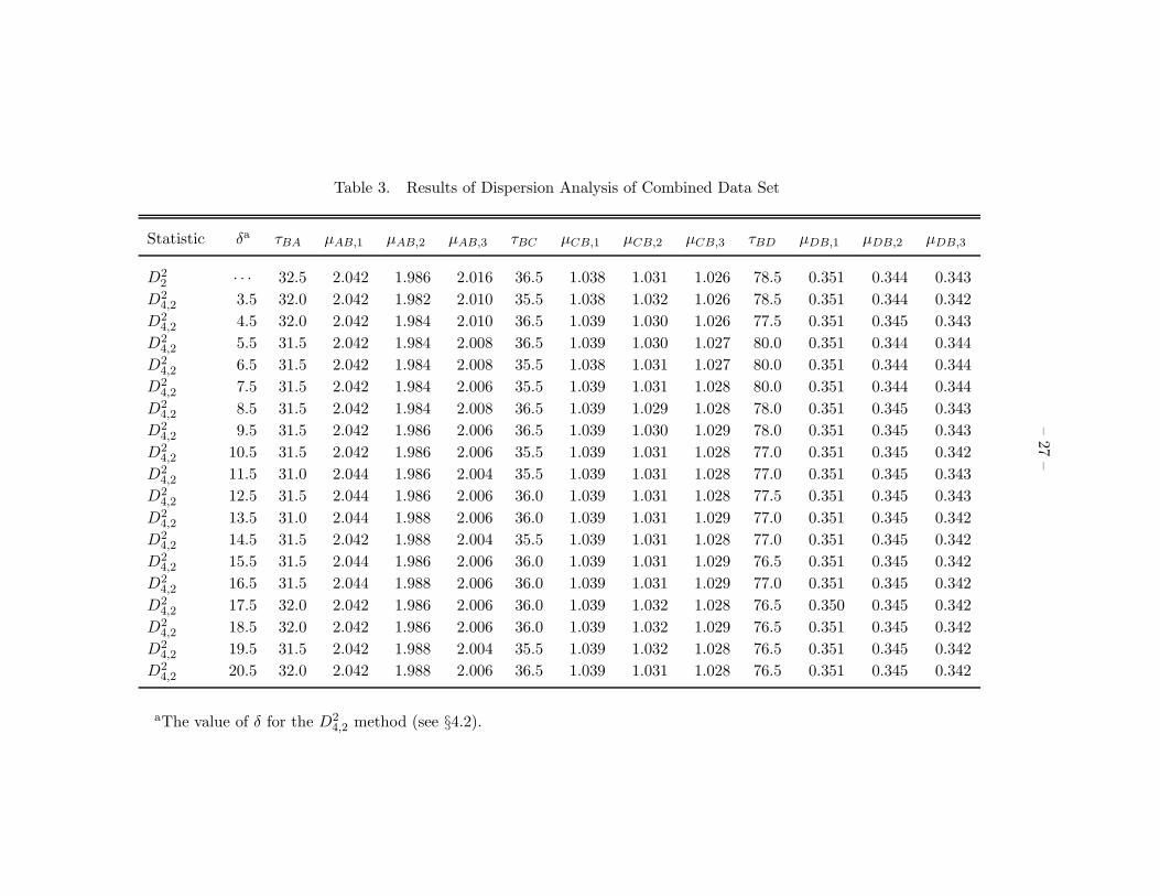
which gave the lowest dispersion. In order to ascertain the robustness of the derived time delays,
we repeated the D24,2 method with a range of values for δ and compared the results (Table 3).
Figure 3 shows typical output curves from the dispersion analysis. We show for comparison the
equivalent curves from the Paper I analysis as dashed lines on the plots. Although both sets of
curves give nearly the same time delays, the curves associated with the combined data sets show
much clearer minima.
We have taken the median values of the columns in Table 3 to be the best-fit time delays
and relative magnifications as determined from the data. These values are given in Table 4. The
median time delays are τBA = 31.5 d, τBC = 36.0 d, and τBD = 77.0 d. The time delay ratios are
(τBD/τBA) = 2.44 and (τBD/τBC) = 2.14. These agree well with the values obtained in Paper I.
We performed several consistency checks on the derived delays. First, we computed all possible
delays between a leading component and a trailing component, using the dispersion methods listed
in Table 3. The median values obtained for these delays were τAC = 2.5 d, τAD = 45.5 d, and
τCD = 44.0 d. These delays are consistent within the uncertainties (§5) with the three delays
calculated above. Secondly, we computed the delays between component B and the other three
components using the χ2-minimization technique described in Paper I, which requires that the
input light curves be interpolated onto a regularly-spaced grid. The χ2-minimization results were
consistent with the dispersion method values, but had more scatter about the median values. The
increased scatter is probably due to small biases introduced by the various methods of interpolating
the input light curves. The final check was to combine the input light curves by shifting the A, C,
and D curves by the appropriate time delays and magnifications and then combining them with the
unshifted B light curve. The resulting composite curves are shown in Figures 4–6. The composite
curves show that the major features, and many of the minor features, in each of the individual light
curves are reproduced in the other light curves at the proper times, giving additional confidence
that the measured delays are the correct ones.
5. Uncertainties on Measured Delays
We have estimated the uncertainties on the time delays and relative magnifications through
Monte Carlo simulations. This is the same method that was used in Paper I. To summarize,
we smoothed each of the composite curves (Figures 4–6) to create the input “true” light curves
for the simulations. One “true” light curve was generated for each season, using the best-fit
relative magnifications appropriate for that season. The delays used for each season were the
global time delays derived from the combined analysis (see Table 4 for the input delays and relative
magnifications). The smoothing method used to generate the “true” curves from the composites was
the variable-width boxcar technique described in Paper I, with five points in the smoothing window.

– 12 –
Fig. 3.— Dispersion spectra from comparison of the light curves of components B and A (left
panel), B and C (middle panel), and B and D (right panel). The spectra were calculated with the
D24 method with δ = 5.5 days (see §4.2). The curve minima, marked with vertical dotted lines,
indicate the time delays. The solid curves represent the results from analysis of the combined data
sets from all three seasons, while the dashed curves represent the results from season 1 alone.

– 13 –
Fig. 4.— Composite light curve constructed from the recalibrated data from season 1. The light
curves for components A, C, and D have been shifted by the time delays and relative magnifications
given in Table 4 and overlaid on the component B light curve. The resulting curve was then nor-
malized by its mean value. Component D is the faintest image and thus the fractional measurement
errors in its flux density are larger than those of the other components. The data points associated
with the four components are denoted by open diamonds (red) for A, filled squares (blue) for B,
filled triangles (black) for C, and open circles (green) for D. The vertical scale is chosen to match
those used in Figures 5 and 6.

– 14 –
Fig. 5.— Same as Figure 4, but for the data from season 2.

– 15 –
Fig. 6.— Same as Figure 4, but for the data from season 3.

– 16 –
The simulated light curves were created by adding a Gaussian-distributed random noise term to
the points on the “true” curves. The widths of the Gaussian distributions, σ, were determined from
the offsets between the measured composite curves and their smoothed counterparts. The values
of σ used ranged from 1.4% to 1.9% of the mean flux densities of the lensed images. We generated
1000 Monte Carlo realizations of the data associated with each season.
The simulated light curves were analyzed with the same code used for the real light curves,
using the D24,2 method. The analysis was repeated using several different values of δ, with no
significant difference in the results. The results in Table 5 were obtained for δ = 4.5d. One
advantage of the method used to analyze the monitoring data is that it yielded not only the time
delays derived from the entire combined data set, but also the delays derived from each season
individually. Thus, the effectiveness of the combined analysis can be evaluated. The distributions
of time delays recovered from the simulations is shown in Figure 7, where the first three figures
show the analyses of the individual seasons and the fourth shows the results from the combined
data sets. The figures show that the distributions are non-Gaussian and that the season 2 data
set does not constrain the time delays well. The latter result was expected given the nature of the
light curves from that season. However, the analysis of the combined data set yields tight limits on
the time delays, which are approximately a factor of two improvement on the limits derived from
the season 1 data alone. All of the delays are now determined to ±3 d or better (95% CL). The
uncertainties on the delays and magnifications, as well as those on derived quantities, are given in
Table 5.
6. Discussion
6.1. Evidence for Microlensing and Lens Substructure
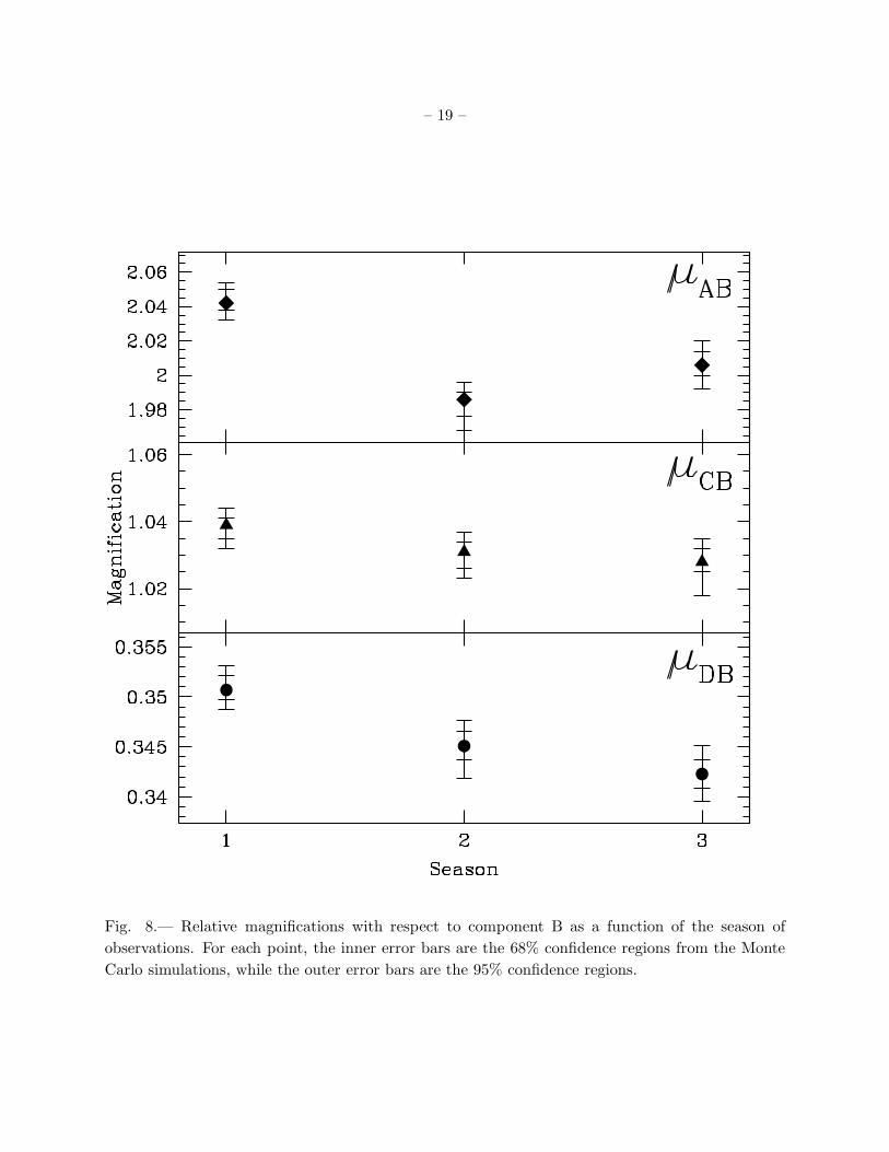
As discussed in §4.2, the component relative magnifications were not constant from seasons 1
to 3. In particular, µAB and µDB decreased by 2% or more during the course of the observations
(Figure 8). Although not large, these changes exceed the 95% confidence limits on the relative
magnifications derived from the Monte Carlo simulations (Table 5), and thus appear to be real.
Similar or more extreme changes in flux ratios are seen in optical monitoring of lens systems (e.g.,
Wozniak et al. 2000; Burud et al. 2000). These changes are attributed to microlensing events, where
stars or other massive compact objects in the lensing galaxy change the magnifications of the lensed
images as they move through the galaxy. For many years, it was thought that radio observations of
gravitational lens systems should be unaffected by microlensing because the angular sizes of compact
radio cores, typically on the order of a milliarcsecond, are much larger than the microarcsecond
lensing cross sections of stars. However, radio monitoring of the lens CLASS B1600+434 has
revealed changes in the component flux ratio that has been attributed to microlensing (Koopmans
& de Bruyn 2000). In the case of B1600+434 the unexpected microlensing was interpreted as being
due to the superluminal motion of a microarcsecond-sized component in the jet of the background

– 17 –
Fig. 7.— Distribution of time delays resulting from dispersion-method analysis of 1000 Monte Carlo
realizations of the component light curves. (a) Season 1 results. (b) Season 2 results. (c) Season 3
results. (d) Results from the analysis of the combined data from all three seasons.

– 18 –
quasar across the complex caustic structure produced by compact objects in the lens galaxy halo
(Koopmans & de Bruyn 2000). The lensed source in the B1608+656 system is the core of a classical
radio double source (Snellen et al. 1995). Thus, it is certainly possible that there are extremely
compact jet components associated with B1608+656 as well. On the other hand, the changes in
the flux density ratios may have other explanations, such as scintillation. However, because we
have monitored the system at only one frequency, we do not have the clear discriminant between
microlensing and scintillation that multifrequency monitoring provides (Koopmans & de Bruyn
2000). With properly designed future observations, it may be possible to determine the cause of
the changing flux density ratios in this system.
We note that, whatever the cause of the variability in the relative magnifications, it may also
be necessary to invoke the presence of substructure in the B1608+656 lensing galaxies to explain the
observed flux densities of the images. Simple, or even fairly complex, lens models of the B1608+656
system have not been able to properly reproduce all of the observed flux density ratios (Paper II;
Myers et al. 1995). As we noted in Paper II, this discrepant magnification could be produced by
perturbations to the smooth mass distributions assumed for the lensing galaxies. The presence of
such substructure has been invoked to explain similarly discrepant flux ratios in other four-image
lenses, although in those cases the incongruous ratios were those between bright merging images.
In some cases, the substructure has been interpreted as globular clusters or plane density waves
(Mao & Schneider 1998). Recently, several papers have suggested that the substructure is due to
the small dark matter satellite halos expected from CDM structure-formation models (e.g., Metcalf
& Madau 2001; Chiba 2002; Dalal & Kochanek 2002).
6.2. Determination of H0 with B1608+656
To determine H0 from a lens system, the measured time delays are combined with those pre-
dicted by the model. The predicted delays depend on the values of the fundamental cosmological
parameters, so one must assume a cosmological model. Specifically, the model delays are propor-
tional to (DℓDs)/Dℓs where Dℓ, Ds, and Dℓs are the angular diameter distances from the observer
to the lens, from the observer to the source, and from the lens to the source, respectively. The
angular diameter distances are functions of H0, Ωm, and ΩΛ, as well as the redshifts of the lens and
the background source. We assume (ΩM ,ΩΛ) = (0.3,0.7) for the rest of this paper. In comparison
to this assumed cosmology, the value of H0 derived from this lens system will change by no more
than ∼6% in both flat and open cosmological models with 0.1 < ΩM < 1.0. As specific examples,
the values of H0 discussed below should be scaled by a factor of 1.02 if (ΩM ,ΩΛ) = (0.3, 0.0) and
a factor of 0.94 if (ΩM ,ΩΛ) = (1.0, 0.0).
The considerable improvement in the accuracy of the measured time delays between the three
image pairs in B1608+656 warrants an update of the lens model of this system, first presented in
Paper II. Multiple time delays in a single lens system add additional constraints on the lens model,
and an improvement in their accuracy could therefore lead to a change of the lens model and a
– 19 –
Fig. 8.— Relative magnifications with respect to component B as a function of the season of
observations. For each point, the inner error bars are the 68% confidence regions from the Monte
Carlo simulations, while the outer error bars are the 95% confidence regions.

– 20 –
change of the inferred Hubble Constant. Our models are based on the lensmodel package developed
by Keeton (2001), but the results are consistent with those based on the code used in Paper II. We
emphasize that the models presented here are only an update of the isothermal lens mass models in
Paper II and that a much more detailed mass model will be presented in a forthcoming publication,
where we fully exploit additional data on the system (see §7).
For the lens modeling in this paper, we use the same constraints as in Paper II. We use the
VLBI image positions with formal 1σ errors listed in Paper II. Because the flux density ratios
appear to slowly change in time (§4.2), even after the time-delay correction of the light curves,
we widen the error bars to 20% on the flux density ratios to err on the side of caution. We use
the improved time delays presented in this paper with 1.5 d errors (68% CL). We use singular
isothermal ellipsoid (SIE) mass models for both lens galaxies (G1 and G2; see Paper II for details)
and center them on the galaxy centroids measured from Hubble Space Telescope (HST) images
obtained with the F555W, F814W, and F160W filters. The three centroids differ by amounts that
are significant, which could be due to the presence of dust extinction and/or PSF problems. In
addition, it is possible that the two merging lens galaxies are contained within a common dark
matter halo and, thus, that the luminous material may not provide an accurate representation of
the shape and centroid(s) of the mass distribution. These issues will be examined in more detail
in the forthcoming publication. Here, we present models for the centroids from the F814W and
F160W images; we reject the model based on the F555W centroids because it produces an extra
image of the background source that is not seen in the data. As already shown in Paper II, the
differences in the centroids do not strongly affect the inferred value of H0, although the cause of
the wavelength-dependent shifts in position is something that requires further study.
The mass distributions of G1 and G2 are allowed to have a free mass scale (i.e., velocity
dispersion), position angle, and ellipticity. At this point no external shear is allowed. Both lens
galaxies are assumed to be at the same redshift. The results of the updated lens models and inferred
values of H0 are listed in Table 6. We note that these models are equivalent to models I and II in
Table 3 of Paper II, in spite of using completely independent modeling codes in the two papers.
We also note that, in order to compare the models produced by the two codes, it is important to
understand how the mass scales in the models depend on the projected axial ratio of the lensing
galaxies, q. We find that the relation between the quantities representing the lens strengths, σ
in Paper II and b′ in Table 6, is given by b′√
1 + q2 ∝ √q σ2. Using this relation, we find that
the mass scales presented in Paper II and in Table 6 are also equivalent and that the mass ratio
between galaxies G1 and G2 is (M1/M2) ∼ (b′1/b′
2)2 ∼ 3. This large mass ratio avoids the creation
of additional images between galaxies G1 and G2.
We have also modeled the system with an allowance for an external shear (γext). The addition
of shear to the models in Table 6 leads to a considerable decrease in the value of χ2, for γext ∼ 0.1.
However, the number of free parameters in the models increases to 11 (including H0), and the
models are less well constrained than the models with no shear. Additionally, although there are
several small galaxies in the field around B1608+656, there is no evidence for a more massive group

– 21 –
or cluster that could yield a 10% external shear, as for example in the case of PG1115+080 (Kundic
et al. 1997a; Tonry 1998). Thus, we think that the true external shear (i.e., a constant shear not
due to the lens galaxies themselves) is unlikely to be as high as 10% and that a revision of the
galaxy mass models is more likely required.
The formal statistical errors on H0 in the models are ±1 km s−1 Mpc−1 and ±2 km s−1 Mpc−1
for the 1σ and 2σ confidence limits, respectively. In Paper II we estimated that the range of rea-
sonable variations in the shapes of the mass profiles of the lens galaxies contributed an additional
uncertainty of 30% to the determination of H0 from this system. This estimate may be overly con-
servative, given the small scatter in mass profile slopes seen in other lens galaxies (§6.3). However,
given the complex nature of the lens system and the uncertain positions of the lensing galaxies,
we will use this estimate of the systematic modeling uncertainties in this paper. In §7, we discuss
methods by which the modeling uncertainties for this system may be reduced.
We note that an alternative and independent approach to lens modeling, namely the non-
parametric method developed by Williams & Saha (2000), produces estimates of H0 and its sys-
tematic uncertainties that are similar to those determined in this paper. In comparison to the more
frequently used analytic modeling approaches, the non-parametric method has the advantage of
making fewer assumptions about the form of the mass distribution in the lensing galaxy or galax-
ies. Thus, it is possible to explore a larger region of the model space than is usually done with
single analytic models and, as a consequence, to obtain a perhaps more realistic estimate of the
uncertainties due to modeling. On the other hand, given the additional freedom in model parame-
ters, the non-parametric approach may produce some descriptions of the lensing galaxy that do not
have a physical meaning, in spite of the constraints introduced to produce realistic galaxy models.
Therefore, a straightforward interpretation of the results may be difficult. Williams & Saha (2000)
applied their approach to the B1608+656 system, using the image positions and time delays as
constraints. The time delays used by Williams & Saha (2000) were from an early analysis of the
Season 1 data and differ slightly from those found in this paper. However, these small differences
should not significantly affect the resulting values of H0. Williams & Saha (2000) found that ∼90%
of their model reconstructions produced values of H0 between 50 and 100 km s−1 Mpc−1. They
also applied their non-parametric method to PG1115+080 and the results were combined with the
B1608+656 results to produce H0 = 61 ± 11 (±18) km s−1 Mpc−1at 68% (90%) confidence, for
(ΩM ,ΩΛ) = (1.0, 0.0). For the cosmological model adopted in this paper, their value of H0 would
change to 65 km s−1 Mpc−1, consistent with our results.
6.3. Comparison to Determinations of H0 with Other Lens Systems
Time delays have been measured in 11 lens systems, with the B1608+656 delays being among
those with the smallest uncertainties. Unfortunately, the determination of H0 from lenses is not
as clean as one might have hoped. For nearly every lens with a measured time delay, more than

– 22 –
one model has been used to fit the data. Often the resulting values of H0 are quoted with small
formal errors that, when taken at face value, make different determinations of H0 with the same
lens system mutually exclusive at high levels of significance. These discrepant values of H0 arise
because observations of most lens systems do not tightly constrain the mass distribution of the
lens, and there is a degeneracy between the steepness of the lens mass profile and the derived value
of H0 (e.g., Paper II; Williams & Saha 2000; Witt, Mao, & Keeton 2000).
Although it may not be possible to determine the radial mass profile in many individual lens
systems, there are indications that lensing galaxies may follow a nearly universal mass profile. It is,
for example, possible to assume that all lenses must give consistent determinations of H0 and then
use the time-delay measurements to obtain information about the mass distribution in the lenses.
Kochanek (2002b) has performed this experiment on a sample of five lens systems with measured
delays. He finds that, in order to produce the same value of H0, the mass surface density properties
of the lensing galaxies must differ by only very small amounts. Furthermore, several independent
lines of investigation indicate that not only are the mass distributions in many lenses similar, but
that the mass profiles are close to isothermal. These approaches have used models that incorporate
more data than the standard two or four image positions and fluxes. The additional inputs make
it possible to place tight limits on the slope of the mass distribution. The additional constraints
may come from full or partial Einstein rings (e.g., Kochanek 1995; Keeton et al. 2000; Kochanek et
al. 2001), complex structure in the background source that in lensed into a ring-like configuration
(Cohn et al. 2001), stellar dynamics (Treu & Koopmans 2002; Koopmans & Treu 2002), or the
orientations of mas-scale jets seen in very high angular resolution radio maps (Rusin et al. 2002).
Although it should not be concluded that all lens galaxies have nearly isothermal mass distributions,
it may be that the range of mass profile slopes present in lensing galaxies is significantly smaller than
what is allowed by the constraints in most individual lens systems with time delay measurements.
If further observations strengthen these conclusions, then the contribution of a major source of
systematic error in lens-derived measurements of H0 may be significantly decreased.
The mass profile of the main lensing galaxy is not the only source of uncertainty in the de-
termination of H0 from a lens system. Another factor enters if there is a cluster or massive group
associated with the primary lensing galaxy. The inclusion of the effects of the cluster can vastly
complicate the lens model. The case of the first lens to be discovered, Q0957+561, is instructive.
Despite many years of intensive observational and modeling efforts, no definitive model has been
developed. For an excellent discussion of the wealth of historical models of this system, see Keeton
et al. (2000). Clusters have also been discovered in association with RX J0911.4+0551 (Kneib,
Cohen, & Hjorth 2000; Morgan et al. 2001) and possibly SBS 1520+530 (Faure et al. 2002). In
addition, compact groups of galaxies have been discovered in association with several lens systems
(e.g., Kundic et al. 1997a,b; Tonry 1998; Tonry & Kochanek 1999, 2000; Fassnacht & Lubin 2002;
Rusin et al. 2001), although their effects on the lensing properties of the systems are much smaller
than those of clusters. Still another problem in the determination of H0 from gravitational lens
systems arises if the location of the lensing galaxy is not known, as is the case in B0218+357 (Lehar

– 23 –
et al. 2000).
In spite of the possible problems mentioned above, the gravitational lens method is attractive
because many of the systematic errors affecting the determination of H0 with one lens system are
different from those affecting other systems. Thus, it should be possible to obtain a global mea-
surement of H0 with small uncertainties by averaging the measurements from many lens systems.
This is in contrast to the distance-ladder techniques in which many of the systematic uncertainties
affect all distance determinations in the same sense. The major problem with the gravitational-lens
method is that the number of lens systems with measured time delays is still small. Even though
the number of systems for which delays have been measured has increased substantially over the
last few years, some of the delays are not measured to high precision. In addition, lens models for
some systems are viewed with suspicion due to problems such as those mentioned in the previous
paragraph. Thus, efforts to determine a global value of H0 often exclude a significant fraction of
systems with time-delay measurements. Recent attempts have been limited to samples consist-
ing of five or fewer lenses, and have obtained global values of H0 ranging from ∼50 to ∼75 km
s−1 Mpc−1 (e.g., Paper II; Schechter 2000; Kochanek 2002a). With such small sample sizes, the
mean H0 obtained can easily be biased by unknown factors affecting one or two of the lens systems.
It is thus crucial to measure time delays in more lens systems in order to obtain a robust global
determination of H0 from lenses.
6.4. Comparison to Determinations of H0 with Other Methods
There are, of course, methods for measuring H0 that are completely independent of the lens-
derived values. These include the traditional distance-ladder methods in which Cepheid-based
distances are used to calibrate secondary distance indicators. The HST Key Project combined
several secondary distance measurement methods to obtain a final value of H0 = 72±3(1σ)±7 (sys)
km s−1 Mpc−1 (Freedman et al. 2001). Using an analysis of Cepheid-calibrated distances to Type
Ia supernovae, Parodi et al. (2000) derived H0 = 59± 6km s−1 Mpc−1 (2σ random errors combined
with estimated systematic effects). The use of the Sunyaev-Zeldovich (SZ) effect is another approach
that, like the gravitational lens method, is independent of the distance-ladder approach. In recent
work by Mason, Myers, & Readhead (2001), the average measurement obtained from a flux-limited
sample of clusters was H0 = 66+14−11(1σ)±14 (sys) km s−1 Mpc−1. The global values of H0 determined
from lenses, the SZ effect, and traditional distance-ladder methods are broadly consistent with each
other and with the H0 determined from B1608+656. The sources of systematic error in each of
these methods are different. Therefore, if the methods all produced values of H0 that were in good,
rather than broad, agreement, the confidence that the correct value had been measured would
be increased. It is important that steps be taken to understand the systematic errors affecting
each method and to attempt to reduce those errors. The systematic errors associated with the
gravitational lens method may be reduced if time delays can be measured and mass profiles can be
determined in significantly larger samples of lens systems.

– 24 –
7. Summary and Future Work
In this paper we have presented data obtained during three seasons of monitoring of the
B1608+656 gravitational lens system. An analysis of the combined data sets from the three seasons
has led to an improvement of factors of two to three in the precision of the three time delays
measured. In addition, there is evidence that the relative magnifications of the lensed images are
changing. Because these relative magnifications should be independent of the absolute flux density
calibration, the observed changes may imply that at least one of the images is being affected by
microlensing. If this is the case, B1608+656 would be only the second lens system in which radio
microlensing has been detected. A combination of the time delays with revised lens models yields
H0 = 61–65 km s−1 Mpc−1, depending on the positions used for the lensing galaxies, for (ΩM ,ΩΛ)
= (0.3,0.7). These values decrease by 6% for (ΩM ,ΩΛ) = (1.0,0.0). The uncertainties on H0 due
to the time delay measurements are ±1 (±2) km s−1 Mpc−1 for the 1σ (2σ) confidence intervals.
Now that the time delays have been determined to 4–10% (95% CL), the dominant source of error
in the determination of H0 with the B1608+656 system comes from the lens model. The model
uncertainties are on the order of ±15 km s−1 Mpc−1.
There are two lensing galaxies within the ring of images in the B1608+656 system, which
presents a challenge to the modeling process. Because of the disturbed nature of the system,
discussions of general time delay properties and the derivation of H0 from lenses have tended to
discard B1608+656 from the samples being considered (e.g., Witt, Mao, & Keeton 2000; Kochanek
2002a). However, the B1608+656 system does have the advantage of having a nearly complete
Einstein ring that is seen in optical and infrared HST images (Jackson et al. 1997; Surpi & Blandford
2002). It thus may be possible to use the ring data to constrain the mass profile slopes of the lensing
galaxies. Techniques to incorporate the Einstein ring data into the B1608+656 model have been
described by Blandford, Surpi, & Kundic (2001) and Kochanek et al. (2001). The observed ring is
faintest between components B and D, and is not detected at high significance in this region in the
available HST images (Kochanek et al. 2001; Surpi & Blandford 2002). In order to fully exploit
the ring modeling techniques, it is critical to obtain deeper HST images of the system so that the
ring emission can be more clearly separated from the noise. The availability of the new Advanced
Camera for Surveys, with improved sensitivity and a finer pixel scale compared to the Wide Field
Planetary Camera 2, and the revived Near Infrared Camera and Multi-Object Spectrometer will
greatly aid in the effort to get such images. In addition to the analysis of Einstein ring emission,
information about the stellar dynamics of lensing galaxies can place strong constraints on the mass
distribution of the lens (Treu & Koopmans 2002; Koopmans & Treu 2002). We have obtained
high resolution spectra of the B1608+656 system with the Echelle Spectrograph and Imager on
the Keck II telescope with which we will investigate the dynamics of the lensing galaxies. A
full analysis of the Einstein ring structure, the environment surrounding the lens system, and the
stellar kinematics should help to break the remaining degeneracies in the model (e.g., precise galaxy
positions, external shear, radial mass profile, etc.) and, thus, significantly reduce the uncertainties
on H0 due to the lens model.

– 25 –
An observing program of this complexity could not have been completed without the assistance
of the NRAO staff. Their efforts in keeping the VLA running smoothly and their advice on the
structure of the observing program were invaluable. We especially thank Meri Stanley, Jason
Wurnig, and Ken Hartley for making sure that all epochs had been properly scheduled. We are
also grateful to the VLA operators for implementing the observing program. For useful discussions
and comments on the paper, we thank Ingunn Burud, Stefano Casertano, Tim Pearson, Lori Lubin,
Steve Myers, Frazer Owen, Rick Perley, Ken Sowinski, and Greg Taylor. We thank the anonymous
referee for suggestions that improved the paper.

– 26 –
Table 2. Component Positions and Mean Flux Densities
xa ya < S1 > < S2 > < S3 >
Component (arcsec) (arcsec) (mJy) (mJy) (mJy)
A 0.000 0.000 34.1 21.8 22.8
B −0.738 −1.962 16.8 10.6 11.6
C −0.745 −0.453 17.3 11.3 11.6
D 1.130 −1.257 5.9 4.0 3.7
aComponent positions are given in Cartesian rather than astro-
nomical coordinates.
–27
–
Table 3. Results of Dispersion Analysis of Combined Data Set
Statistic δa τBA µAB,1 µAB,2 µAB,3 τBC µCB,1 µCB,2 µCB,3 τBD µDB,1 µDB,2 µDB,3
D22 · · · 32.5 2.042 1.986 2.016 36.5 1.038 1.031 1.026 78.5 0.351 0.344 0.343
D24,2 3.5 32.0 2.042 1.982 2.010 35.5 1.038 1.032 1.026 78.5 0.351 0.344 0.342
D24,2 4.5 32.0 2.042 1.984 2.010 36.5 1.039 1.030 1.026 77.5 0.351 0.345 0.343
D24,2 5.5 31.5 2.042 1.984 2.008 36.5 1.039 1.030 1.027 80.0 0.351 0.344 0.344
D24,2 6.5 31.5 2.042 1.984 2.008 35.5 1.038 1.031 1.027 80.0 0.351 0.344 0.344
D24,2 7.5 31.5 2.042 1.984 2.006 35.5 1.039 1.031 1.028 80.0 0.351 0.344 0.344
D24,2 8.5 31.5 2.042 1.984 2.008 36.5 1.039 1.029 1.028 78.0 0.351 0.345 0.343
D24,2 9.5 31.5 2.042 1.986 2.006 36.5 1.039 1.030 1.029 78.0 0.351 0.345 0.343
D24,2 10.5 31.5 2.042 1.986 2.006 35.5 1.039 1.031 1.028 77.0 0.351 0.345 0.342
D24,2 11.5 31.0 2.044 1.986 2.004 35.5 1.039 1.031 1.028 77.0 0.351 0.345 0.343
D24,2 12.5 31.5 2.044 1.986 2.006 36.0 1.039 1.031 1.028 77.5 0.351 0.345 0.343
D24,2 13.5 31.0 2.044 1.988 2.006 36.0 1.039 1.031 1.029 77.0 0.351 0.345 0.342
D24,2 14.5 31.5 2.042 1.988 2.004 35.5 1.039 1.031 1.028 77.0 0.351 0.345 0.342
D24,2 15.5 31.5 2.044 1.986 2.006 36.0 1.039 1.031 1.029 76.5 0.351 0.345 0.342
D24,2 16.5 31.5 2.044 1.988 2.006 36.0 1.039 1.031 1.029 77.0 0.351 0.345 0.342
D24,2 17.5 32.0 2.042 1.986 2.006 36.0 1.039 1.032 1.028 76.5 0.350 0.345 0.342
D24,2 18.5 32.0 2.042 1.986 2.006 36.0 1.039 1.032 1.029 76.5 0.351 0.345 0.342
D24,2 19.5 31.5 2.042 1.988 2.004 35.5 1.039 1.032 1.028 76.5 0.351 0.345 0.342
D24,2 20.5 32.0 2.042 1.988 2.006 36.5 1.039 1.031 1.028 76.5 0.351 0.345 0.342
aThe value of δ for the D24,2 method (see §4.2).

– 28 –
Table 4. Measured Quantities
Component τa µ1b µ2
b µ3b
A 31.5 2.042 1.986 2.006
C 36.0 1.039 1.031 1.028
D 77.0 0.351 0.345 0.342
aTime delay between component in table
and component B, in days.
bRelative magnification of component in
table with respect to component B, for season
1, 2, or 3.
Table 5. Parameter Confidence Intervals from Combined Analysis
Quantity Input Value 68% Confidence Interval 95% Confidence Interval
τBA 31.5 30.5–33.5 29.0–34.5
τBC 36.0 34.5–37.5 33.5–38.5
τBD 77.0 76.0–79.0 74.0–81.0
µAB,1 2.042 2.038–2.050 2.032–2.054
µAB,2 1.986 1.976–1.990 1.968–1.996
µAB,3 2.006 2.000–2.014 1.992–2.020
µCB,1 1.039 1.035–1.041 1.032–1.044
µCB,2 1.031 1.027–1.034 1.023–1.037
µCB,3 1.028 1.025–1.032 1.021–1.035
µDB,1 0.351 0.350–0.352 0.349–0.353
µDB,2 0.345 0.344–0.347 0.342–0.348
µDB,3 0.342 0.341–0.344 0.340–0.345
(τBD/τBA) 2.44 2.37–2.47 2.34–2.51
(τBD/τBC) 2.14 2.12–2.19 2.09–2.22

– 29 –
Table 6. Mass Model Parameters
xca yc
a b′ P.A.b xsa ys
a H0
Filter (arcsec) (arcsec) (arcsec) q (deg) (arcsec) (arcsec) (km s−1 Mpc−1) χ2
F814W +0.521 −1.062 0.68 0.88 +71.8 +0.060 −1.090 65 43
−0.293 −0.965 0.39 0.39 +53.1
F160W +0.446 −1.063 0.69 0.91 −58.0 +0.058 −1.103 61 196
−0.276 −0.937 0.36 0.31 +53.8
aPositions are given in Cartesian rather than astronomical coordinates.
bPosition angles are defined in the astronomical convention, in degrees measured east of north.
Note. — Lens models for B1608+656 consisting of two SIE mass distributions with no external shear.
Columns 2–3 indicate the galaxy centroids measured in the HST images obtained with the listed filter;
columns 4–6 indicate the lens strength (see alpha models in Keeton 2001), axial ratio, and position angle
of the SIE mass distribution; columns 7–8 indicate the source position; columns 9–10 indicate the inferred
value of H0 and the model χ2 value. The values of H0 are quoted for (ΩM ,ΩΛ) = (0.3, 0.7). Every
first/second line indicates the parameters for galaxy G1/G1.

– 30 –
REFERENCES
Barkana, R. 1997, ApJ, 489, 21
Biggs, A. D., Browne, I. W. A., Helbig, P., Koopmans, L. V. E., Wilkinson, P. N., & Perley, R. A.
1999, MNRAS, 304, 349
Blandford, R., Surpi, G., & Kundic, T. 2001, in ASP Conf. Ser. 237, Gravitational Lensing: Recent
Progress and Future Goals, ed. T. G. Brainerd & C. S. Kochanek (San Francisco: ASP), 65
Burud, I., et al. 2000, ApJ, 544, 177
Burud, I., et al. 2002a, A&A, 383, 71
Burud, I., et al. 2002b, A&A, in press (astro-ph/0206084)
Chiba, M. 2002, ApJ, 565, 17
Cohen, A. S., Hewitt, J. N., Moore, C. B., Haarsma, D. B. 2000, ApJ, 545, 578
Cohn, J. D., Kochanek, C. S., McLeod, B. A., & Keeton, C. R. 2001, ApJ, 554, 1216
Dalal, N. & Kochanek, C. S. 2002, ApJ, 572, 25
Fassnacht, C. D., Womble D. S., Neugebauer, G., Browne, I. W. A., Readhead, A. C. S., Matthews,
K., & Pearson, T. J. 1996, ApJ, 460, L103
Fassnacht, C. D., Pearson, T. J., Readhead, A. C. S., Browne, I. W. A., Koopmans, L. V. E.,
Myers, S. T., & Wilkinson, P. N. 1999, ApJ, 527, 498 (Paper I)
Fassnacht, C. D. & Taylor, G. B. 2001, AJ, 122, 1661 (FT01)
Fassnacht, C. D. & Lubin, L. M. 2002, AJ, 123, 627
Faure, C., Courbin, F., Kneib, J. P., Alloin, D., Bolzonella, M., & Burud, I. 2002, A&A, 386, 69.
Freedman, W. L., et al. 2001, ApJ, 553, 47
Gil-Merino, R., Wisotzki, L, & Wambsganss, J. 2002, A&A, 381, 428
Hjorth, J., et al. 2002, ApJ, 572, L11
Jackson, N. J., Nair, S., Browne, I. W. A. 1997, in Observational Cosmology with the New Radio
Surveys, ed. M. Bremer, N. Jackson & I. Perez-Fournon, (Dordrecht: Kluwer) 315
Keeton, C. R., et al. 2000, ApJ, 542, 74
Keeton, C. R. 2001, ApJ, submitted (astro-ph/0102340)
Kneib, J.-P., Cohen, J. G., & Hjorth, J. 2000, ApJ, 544, 35

– 31 –
Kochanek, C. S. 1995, ApJ, 445, 559
Kochanek, C. S., Keeton, C. R., & McLeod, B. M. 2001, ApJ, 547, 50
Kochanek, C. S. 2002a, ApJ, submitted (astro-ph/0204043)
Kochanek, C. S. 2002b, ApJ, submitted (astro-ph/0205319)
Koopmans, L. V. E. & Fassnacht, C. D. 1999, ApJ, 527, 513 (Paper II)
Koopmans, L. V. E. & de Bruyn, A. G. 2000, A&A, 358, 793
Koopmans, L. V. E., de Bruyn, A. G., Xanthopoulos, E., & Fassnacht, C. D. 2000, A&A, 356, 391
Koopmans, L. V. E. & Treu, T. 2002, ApJ, submitted (astro-ph/0205281)
Kundic, T. et al. 1995, ApJ, 455, L5
Kundic, T., Cohen, J. G., Blandford, R. D., & Lubin, L.M. 1997a, AJ, 114, 507
Kundic, T., Hogg, D. W., Blandford, R. D., Cohen, J. G., Lubin, L. M., & Larkin, J. E. 1997b,
AJ, 114, 2276
Kundic, T. et al. 1997c, ApJ, 482, 75
Lehar, J, Falco, E. E., Kochanek, C. S., McLeod, B. A., Munoz, J. A., Impey, C. D., Rix, H.-W.,
Keeton, C. R., & Peng, C. Y. 2000, ApJ, 536, 584
Lovell, J. E. J., Jauncey, D. L., Reynolds, J. E., Wieringa, M. H., King, E. A., Tzioumis, A. K.,
McCulloch, P. M., & Edwards, P. G. 1998, ApJ, 508, L51
Mao, S. & Schneider, P. 1998, MNRAS, 295, 587
Mason, B. S., Myers, S. T., & Readhead, A. C. S. 2001, ApJ, 555, 11
Metcalf, R. B. & Madau, P. 2001, ApJ, 563, 9
Morgan, N. D., Chartas, G., Malm, M., Bautz, M. W., Burud, I., Hjorth, J., Jones, S. E., &
Schechter, P. L. 2001, ApJ, 555, 1
Myers, S. T., et al. 1995, ApJ, 447, L5
Parodi, B. R., Saha, A., Sandage, A., & Tammann, G. A. 2001, ApJ, 551, 973
Patnaik, A. R., & Narasimha, D., 2001, MNRAS, 326, 1403
Pelt, J., Hoff, W., Kayser, R., Refsdal, S., & Schramm, T. 1994, A&A, 286, 775
Pelt, J., Kayser, R., Refsdal, S., & Schramm, T. 1996, A&A, 305, 97

– 32 –
Pelt, J., Refsdal, S., & Stabell, R. 2002, A&A, in press (astro-ph/0205424)
Refsdal, S. 1964, MNRAS, 128, 307
Rusin, D., et al. 2001, ApJ, 557, 594
Rusin, D., Norbury, M., Biggs, A. D., Marlow, D. R., Jackson, N. J., Browne, I. W. A., Wilkinson,
P. N., & Myers, S. T. 2002, MNRAS, 330, 205
Schechter, P. L. 2000, to appear in ASP Conf. Ser., New Cosmological Data and the Values of
the Fundamental Parameters, ed. A. Lasenby, A. Wilkinson, & A. W. Jones (San Francisco:
ASP) (astro-ph/0009048)
Schechter, P. L., et al. 1997, ApJ, 475, L85
Shepherd, M. C. 1997, in ASP Conf. Ser. 125, Astronomical Data Analysis Software and Systems
VI, ed. G. Hunt & H. E. Payne, (San Francisco: ASP), 77
Snellen, I. A. G., de Bruyn, A. G., Schilizzi, R. T., Miley, G. K. & Myers, S. T. 1995, ApJ, 447, L9
Surpi, G. & Blandford, R. D. 2002, ApJ, submitted (astro-ph/0111160)
Tonry, J.L. 1998, AJ, 115, 1
Tonry, J. L. & Kochanek, C. S. 1999, AJ, 117, 2034
Tonry, J. L. & Kochanek, C. S. 2000, AJ, 119, 1078
Treu, T. & Koopmans, L. V. E. 2002, ApJ, 575, 87
Wiklind, T. & Combes, F. 2001, in ASP Conf. Ser. 237, Gravitational Lensing: Recent Progress
and Future Goals, ed. T. G. Brainerd & C. S. Kochanek (San Francisco: ASP), 155 (astro-
ph/9909314)
Williams, L. L. R. & Saha, P. 2000, AJ, 119, 439
Witt, H. J., Mao, S., & Keeton, C. R. 2000, ApJ, 544, 98
Wozniak, P. R., Udalski, A., Szymanski, M., Kubiak, M., Pietrzynski, G., Soszynski, I., & Zebrun,
K. 2000, ApJ, 540, L65
This preprint was prepared with the AAS LATEX macros v5.0.