A Cost Model for 3D Woven Preforms - MDPI

J. Compos. Sci. 2022, 6, 18. https://doi.org/10.3390/jcs6010018 www.mdpi.com/journal/jcs

Article

A Cost Model for 3D Woven Preforms

James Clarke 1,*, Alistair McIlhagger 1, Dorian Dixon 1, Edward Archer 1, Glenda Stewart 2, Roy Brelsford 2

and John Summerscales 3

1 Engineering Composites Research Centre, Ulster University, Jordanstown BT37 OQB, UK;

[email protected] (A.M.); [email protected] (D.D.); [email protected] (E.A.) 2 Axis Composites Ltd, Airport Road, Belfast BT3 9DZ, UK; [email protected] (G.S.);

[email protected] (R.B.) 3 MAterials and STructures (MAST)/Composites Engineering Research Group, School of Engineering,

Computing and Mathematics (SECaM), University of Plymouth, Plymouth PL4 8AA, UK;

[email protected]

* Correspondence: [email protected]

Abstract: Lack of cost information is a barrier to acceptance of 3D woven preforms as reinforcements

for composite materials, compared with 2D preforms. A parametric, resource-based technical cost

model (TCM) was developed for 3D woven preforms based on a novel relationship equating man-

ufacturing time and 3D preform complexity. Manufacturing time, and therefore cost, was found to

scale with complexity for seventeen bespoke manufactured 3D preforms. Two sub-models were

derived for a Weavebird loom and a Jacquard loom. For each loom, there was a strong correlation

between preform complexity and manufacturing time. For a large, highly complex preform, the Jac-

quard loom is more efficient, so preform cost will be much lower than for the Weavebird. Provided

production is continuous, learning, either by human agency or an autonomous loom control algo-

rithm, can reduce preform cost for one or both looms to a commercially acceptable level. The TCM

cost model framework could incorporate appropriate learning curves with digital twin/multi-vari-

ate analysis so that cost per preform of bespoke 3D woven fabrics for customised products with low

production rates may be predicted with greater accuracy. A more accurate model could highlight

resources such as tooling, labour and material for targeted cost reduction.

Keywords:3D woven fabrics; preform; complexity; cost model; learning; Weavebird; Jacquard

1. Introduction

3D woven composites have promising growth prospects in a wide range of markets

[1,2]. They possess superior mechanical properties in some respects compared with con-

ventional 2D preforms, for example a composite made from a non-crimp 0, 90 2D rein-

forcing fabric of interlacing orthogonal sets of warp and weft tows, with the warp tows at

0degrees running along the length of the weaving loom and the weft tows at 90degrees to

the warp tows [3]. However, acceptance of 3D woven composites has been difficult in

sectors such as aerospace which increasingly demand lower-cost materials with mechan-

ical performance at least the same or greater than for 2D laminates. Table 1 compares a 0,

90 2D non-crimp fabric composite and a 3D woven composite.

At high production rates, for most manufacturing operations, material cost domi-

nates other resources such as tooling, capital and labour, while tooling and labour costs

dominate for bespoke manufacturing [4,5]. Dry 3D preforms are highly complex materi-

als. There are two types of 3D woven preform: multi-axial and interlock. Interlock pre-

forms are multi-layered fabrics produced by interlacing three sets of fibre tows in a spe-

cialised weaving machine. A general definition of a 3D warp interlock fabric was pro-

posed to better describe the position of the various yarns located inside the 3D woven

structure [6].

Citation: Clarke, J.; McIlhagger, A.;

Dixon, D.; Archer, E.; Stewart, G.;

Brelsford, R.; Summerscales, J. A

Cost Model for 3D Woven Preforms.

J. Compos. Sci. 2022, 6, 18.

https://doi.org/10.3390/jcs6010018

Received: 6 December 2021

Accepted: 31 December 2021

Published: 5 January 2022

Publisher’s Note: MDPI stays neu-

tral with regard to jurisdictional

claims in published maps and institu-

tional affiliations.

Copyright: © 2022 by the authors. Li-

censee MDPI, Basel, Switzerland.

This article is an open access article

distributed under the terms and con-

ditions of the Creative Commons At-

tribution (CC BY) license (http://crea-

tivecommons.org/licenses/by/4.0/).

J. Compos. Sci. 2022, 6, 18 2 of 32

Table 1. Comparison of 2D and 3D woven composites.

2D Woven Composite 3D Woven Composite

Fabric Manufacture Conventional loom for weaving a fabric with in-

terlacing tows in X and Ydirections

Specialist loom for weaving a fabric

with interlacing tows in X, Y and Z di-

rections.

Fabric Structure

Warp tows run along the

length of the weaving loom or X

direction andweft tows run in the

cross direction of the loom, or Y

direction.

Warp, weft and binder tows run in X, Y

and Z directions.

Properties

Higher in-plane-specific stiffness and strength.

Lower delamination resistance.

Lower out-of-plane stiffness andstrength.

Lower in-plane-specific stiffness and

strength.

Higher delamination resistance due to

z-binder.

Higher out-of-plane stiffness and-

strength.

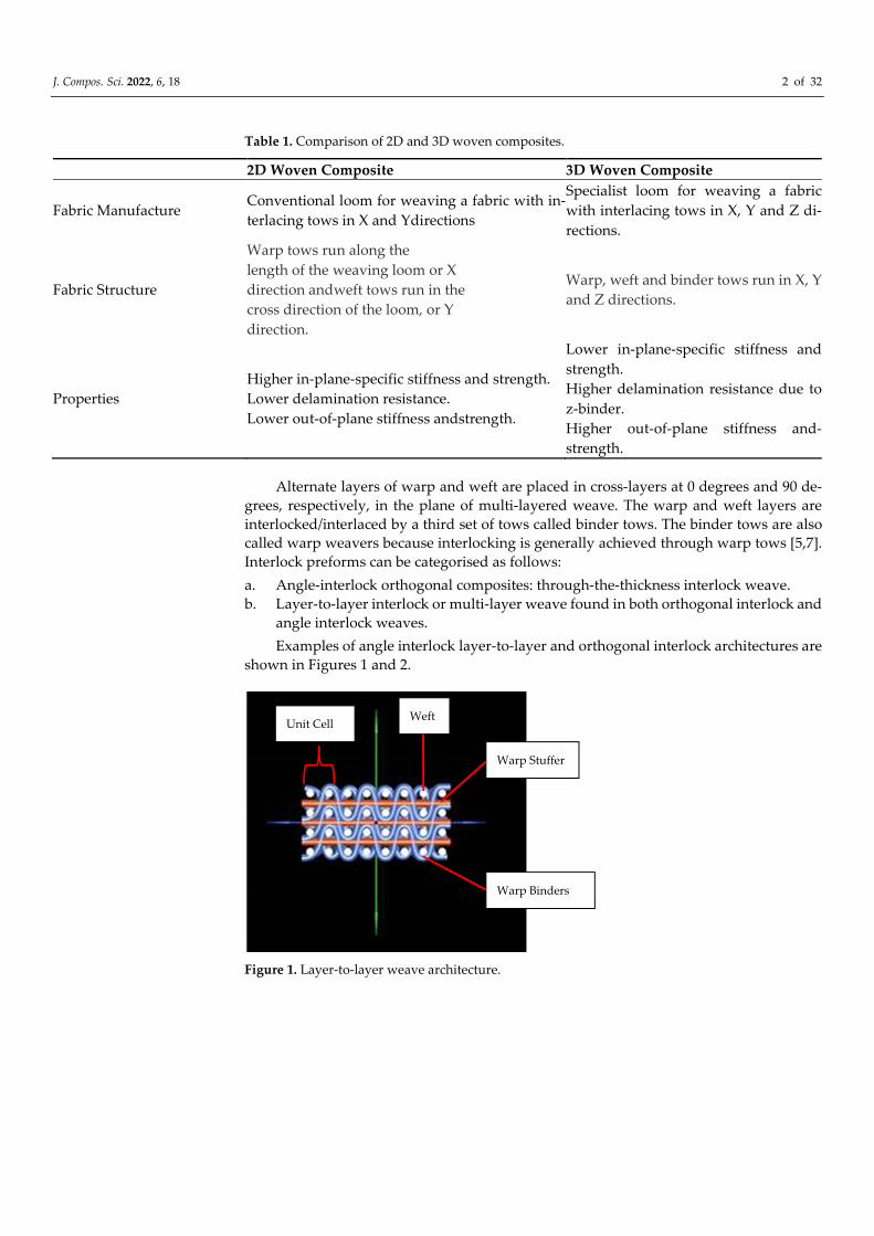
Alternate layers of warp and weft are placed in cross-layers at 0 degrees and 90 de-

grees, respectively, in the plane of multi-layered weave. The warp and weft layers are

interlocked/interlaced by a third set of tows called binder tows. The binder tows are also

called warp weavers because interlocking is generally achieved through warp tows [5,7].

Interlock preforms can be categorised as follows:

a. Angle-interlock orthogonal composites: through-the-thickness interlock weave.

b. Layer-to-layer interlock or multi-layer weave found in both orthogonal interlock and

angle interlock weaves.

Examples of angle interlock layer-to-layer and orthogonal interlock architectures are

shown in Figures 1 and 2.

Figure 1. Layer-to-layer weave architecture.

Warp Stuffer

Warp Binders

Weft Unit Cell

J. Compos. Sci. 2022, 6, 18 3 of 32

Figure 2. Orthogonal weave architecture.

Due to the inherent complexity of the preform manufacturing process, 3D woven

textiles can be expensive [8]. Therefore, knowledge of fabric manufacturing cost is essen-

tial for devising strategies to reduce cost and enable successful competition with long-

established 2D materials. However, while 3D preform commercial cost models are alluded

to [9,10], they are not normally available in the public domain.

The aim of this study was to develop a model to estimate the cost of a hypothetical

3D preform. Data werederived from 17 bespoke 3D preforms manufactured on Weave-

bird and Jacquard weaving looms. A resource-based modelling approach [11] was devel-

oped that took account of the bespoke production of each preform. The model was based

on the principles that cost is determined by resources such as material, tooling, labour and

general overheads [4], and that manufacturing time, and therefore cost, increases with

part complexity [12–14]. Data for resource inputs such as materials, equipment, labour

and energy are approximate values for commercial sensitivity reasons. Technical cost

modelling (TCM) was added as a further refinement in the form of a sub-model detailing

how weaving equipment, labour and energy costs scale with part features such as part

shape and complexity.

Manufacturing cost is not simply the addition of cost elements. How they interact

with each other is a function of learning, which can be either by human agency (for exam-

ple, the combination of textile designer and production operative) or an autonomous ma-

chine control algorithm The study included a description of how preform manufacturing

cost can be reduced once a certain level of learning is attained. For future work, research

into digital twin and/or multi-variate analysis for enhanced learning is proposed as a strat-

egy for reducing the manufacture cost of bespoke preforms made singly or in small

batches.

Two cost models were developed, one for a Weavebird loom (centre closed dobby

shedding mechanism) and another for a Jacquard loom (mechanised production of pat-

terned textiles). In both cases, there was a high correlation, measured by correlation coef-

ficient r2, between manufacturing time and preform complexity for preforms woven on

each loom. Constants derived from time–preform complexity curves for both looms were

input to the model to estimate and compare the cost of a large bespoke 3D preform to be

woven on both looms. Weave tooling and labour accounted for approximately 80% of

preform cost for the bespoke preform. The Jacquard loom is more automated and hence

much more cost effective for large preforms compared to the Weavebird. Learning

through experience will significantly reduce manufacturing weave time and cost per pre-

form.

J. Compos. Sci. 2022, 6, 18 4 of 32

1.1. Literature Review

There are a wide variety of cost models for composite parts by market sector. Huber

[11] proposed three categories for cost modelling of aerospace composites: analogous, par-

ametric, and bottom-up cost estimation. Two possible cost estimation scenarios exist:

Some historic cost data/experience exists for a top-down cost estimation.

Design and process knowledge for a bottom-up, detailed cost calculation.

Essentially, all models are either one of these scenarios or a combination of them. This

generalisation applies equally to cost models in other sectors such as automotive, marine

and construction. The proprietary nature of fundamental data and equations leave most

developed models unusable for third parties.

1.1.1. Manufacturing Cost Models

Esawi [4] provided a comprehensive summary of manufacturing cost model ap-

proaches. The required output of a model will depend on the context. In competitive bid-

ding, the model must deliver a precise, absolute cost as an error of a few percent can make

the difference between profit and loss. When predicting the approximate part cost where

historical data arenot readily available, for example in the early stages of design, a cost

accurate to within a factor of two is acceptable

Function-costing or parametric methods extrapolate the cost of a part that is a variant

of an existing family for which historic cost data already exist. In this case, two conditions

must be met. The part must be a member of a closely related family. Secondly, the family

must have many members with established historical cost data. Similar empirical or cost

scaling methods can be used for part costing which are based on correlations using his-

torical data for estimating the manufacturing cost of a part with given features. The cost

of a new part having certain features made by a given process can be estimated by ana-

lysing cost correlations between previous parts with these features against their size,

shape and complexity and then locating the new part in this cost field. Activity-based

costing methods calculate and sum the cost of each unit operation involved in the manu-

facture of a part. However, a large amount of pre-existing input data arerequired.

Resource-based modellingaccounts for materials, energy, equipment and infrastruc-

ture capital, time, and information resources required for part manufacture. The method

is approximate as values for these inputs are often unknown. TCM is a further refinement

of resource modelling and includes sub-models for how equipment, tooling cost, and pro-

duction rate scale with part features such as part mass, size and complexity. Costs can be

approximate and are isolated, giving TCM flexibility, scalability and adaptability. As

more data become available, detail can be added to the model to improve predictive

power [4].

For TCM calculations based on established data and discussions with experts, Esawi

[4] assumed a complexity factor varying from 1 (minimum complexity) to 5 (maximum

complexity), with a value of 2 assumed for an average complexity factor in calculations of

tooling cost, capital cost and production rate for injection moulding, extrusion and casting

operations. For these operations, tooling cost, capital cost and production rate scale with

part mass and complexity. Tooling and capital vary non-linearly, with exponents for mass

and complexity varying between 0 and 1, implying an economy of scale with increasing

part mass and complexity. Production rate decreases with increase in mass and complex-

ity, so values of exponents for mass and complexity are negative for injection moulding,

extrusion, and casting operations.

Hagnell and Akermo [15] describe a TCM for a generic aeronautical wing in which

costs scale with part features for a given production method. An integrated top-down and

bottom-up approach was employed,depending on available cost data. For a generic aero-

nautical wing, hand layup is normallythe most cost-effective method of those studied for

annual volumes of less than 150 structures per year. For higher production volumes, au-

tomatic tape layup (ATL) followed by hot drape forming (HDF) are the most cost-effective

J. Compos. Sci. 2022, 6, 18 5 of 32

choices. For all production methods, cost per part fell as production rates increased until

material cost dominated at a minimum production rate.

Gutowski et al. [16] derived a series of cost equations incorporating variables and

constants to estimate composite part manufacturing costs for an aircraft structure. The

estimated results fit well with the Advanced Composite Cost Estimating Manual (AC-

CEM) model [11]. However, the system does not account for quality inspection processes.

Verrey et al. [17] studied two resin transfer moulding (RTM) processes for automotive

body-in-white (BIW) structures. An epoxy system was compared with a novel reactive

polyamide 12 (PA12) via characterisation of reaction kinetics and the production of carbon

thermoplastic (TP) fibre floor pan quadrant demonstrators incorporating typical geomet-

rical features. Parametric TCM tools were used to compare the two RTM variants for full

floor-pan production at volumes of 12,500–60,000 parts per year. TCM offered flexibility

together with easy manipulation of processing and economic factors for sensitivity stud-

ies. A 22% increase in cost occurred for the standard TP-RTM cycle versus the epoxy sys-

tem. In-mould cycle time was dominated by thermal cycling of the tool which was re-

quired to reduce component temperature below Tg before demoulding the thermoplastic

part. A study of alternative strategies showed that a reduction in non-crimp fabric scrap

gavemajor cost savings. Cost per part reduced with increase in production volume, with

carbon non-crimp fibre (NCF) material cost accounting for 66% of part cost at a minimum

production volume of 60,000 parts year. At this volume, carbon fibre becomes economic

at a maximum price of €10/kg compared with glass fibre and steel.

Schubel [18] employed TCM to compare the cost of making a 40m wind turbine blade

by handlayup, prepreg, vacuum infusion and resin transfer moulding with automated

manufacturing techniques such as automated tape laying (ATL), automated fibre place-

ment (AFP) and overlay braiding. ATL and AFP reduced manufacturing costs by up to

8% despite the high capital costs of automated equipment. Part size, production volume,

material cost and tooling cost were accounted for. Cost centres were isolated and clearly

indicated the dominance of materials and labour. For the manufacture of a large wind

turbine blade,material deposition in the tool is only one of a string of labour-intensive

processes. A holistic automated blade manufacturing approach is required to see true la-

bour saving benefits.

3D woven fabrics are promising materials for growing market sectors, e.g., wind tur-

bine blades for renewable energy generation [10]. However, high cost is still a major ob-

stacle for uptake of high-performance materials such as carbon fibre. Ennis et al. [19] as-

sessed the commercial viability of cost-competitive carbon fibre composites specifically

suited for the unique loading conditions experienced by wind turbine blades. The wind

industry is costdriven while carbon fibre materials have been developed for the perfor-

mance-driven aerospace industry. Carbonfibre has known benefits for reducing wind tur-

bine blade mass due to significantly improved stiffness, strength and fatigue resistance

per unit mass compared to fibreglass. Novel carbon fibre reinforcements derived from the

textile industry, and characterised using a validated material cost model and mechanical

testing, were studied as potentially more optimal materials for wind turbine blades.

A novel heavy tow textile carbon fibre was compared [19] with commercial carbon

fibre and fibreglass materials in representative land-based and offshore reference wind

turbine blade models. Some advantages of carbon fibre spar caps are observed in reduced

blade mass and improved fatigue life. The heavy tow textile carbon fibre has improved

cost performance over the baseline carbon fibre and performed similarly to commercial

carbon fibre in wind turbine blade design at a significantly reduced cost. The novel carbon

fibre was observed to outperform fibreglass when comparing material cost estimates for

spar caps optimised to satisfy design constraints. The study outlined a route for broader

carbon fibre usage by the wind industry to enable larger rotors that capture more energy

at a lower cost. Heavytow textile carbon fibre cost is estimated at €9.46/kg for an annual

production volume of 2400 tonnes per year, reducing by 43% to€6.88/kg for an increased

annual production volume of 6000 tonnes per year.

J. Compos. Sci. 2022, 6, 18 6 of 32

Fibre-reinforced composites play a key role in automotive applications because of

their high strength to weight and stiffness to weight ratios compared with metals [20]. An

integrated assessment of the durability, reliability and affordability of these materials is

critical for facilitating their inclusion in new designs. A method to develop this assessment

is described for fabricating sheet moulding compound (SMC) parts, together with the con-

cept of Preform Insert Assembly for improved affordability in composite part manufac-

ture.

A computer-aided material selection tool was developed for selecting the most suit-

able carbon fibre-reinforced composite configuration for aircraft structures [21]. The pro-

cedure is based on technical, economic and environmental performance objectives for a

given design, in a multi-disciplinary and multi-objective optimisation scenario.

Carbon-fibre-based composite manufacturing processes have been considered for

automotive body panel applications [22]. A full-scale front wing–fender component was

produced using two composite manufacturing processes, a semi-impregnated (semi-preg)

system and a novel directed fibre preforming–resin transfer moulding process. Both pro-

cesses were compared with an existing stamped steel component for mechanical proper-

ties, weight saving and cost, using a TCM procedure. Mechanical testing demonstrated

that the carbon fibre composite solutions provided 40–50% weight saving for an equiva-

lent bending stiffness compared to steel panels and greatly improved dent resistance. For

the part studied, carbon fibre semi-preg systems offered the lowest-cost process at ap-

proximately500 parts/annum and directed fibre preforming technologies were cheaper,

between 500 and 9000 parts/annum. The steel component was seen to be more cost effec-

tive at volumes above 9000 parts/annum.

A study was conducted to estimate the manufacture cost of a simple component in a

number of different composite materials and by different manufacturing routes [23]. The

materials and routes selected span the range of composites appropriate from general en-

gineering to aerospace applications. A simple methodology is introduced for a compari-

son on the basis of cost-performance efficiency. It is demonstrated that more economic

solutions may often be realised by the choice of ‘expensive’ carbon rather than ‘cheaper’

E-glass as the reinforcing fibre.

The majority of 3D woven preforms currently commercially available are formed by

a 2D weaving process to build a preform with fibres oriented in three dimensions. Multi-

ple insertion 3D differs from traditional weaving and involves 3D fabric formation with

each process cycle, i.e., multi-layers at one time. The successful development and applica-

tion of 3D woven composites will depend on an accurate understanding of the cost drivers

in the manufacturing process. The costs associated with textile preforming are not as

straightforward. A cost model was developed for multiple insertion 3D weaving [24] fo-

cusing on the effects of fabric design, fabric size (thickness and width) and fibresize (linear

density) on setup cost, running production cost and conversion cost.

Despite the limited number of commercial 3D preform weave technologies, the de-

sign window for this class of materials is very broad. Even for one 3D weaving technology,

and restricting fibre inputs to selected standard carbon and glass tows, design flexibility

is still almost limitless. Process modelling, cost modelling, and performance modelling

must all be applied to the design in terms of material, preform and performance in the

final application so that development cycle times can be reduced. A concurrent engineer-

ing approach is described [25] for designing 3D woven fabrics that accounts for manufac-

turing and performance in addition to cost. A case study was presented to demonstrate

that relatively minor design changes can result in very different performance and costs.

The cost-effective manufacture of carbon fibre-reinforced parts in high-wage econo-

mies is a major research goal for industry. An initiative is described [26] to develop a soft-

ware tool for cost prediction in the early design stage to assist optimum process selection

and highlight potential cost reductions.

While advanced composites can significantly reduce aircraft structural weight com-

pared to conventional metal structures, the aerospace industry was reluctant to introduce

J. Compos. Sci. 2022, 6, 18 7 of 32

them to new aircraft. The US Air Force Composites Affordability Initiative [27] found that

the key to affordability in composites was to reduce assembly costs through the integra-

tion and bonding of parts. A partnership between various aerospace companies, the US

Air Force Research Laboratory, and the US Office of Naval Research, was created to de-

velop the materials and technologies required to fly large integrated and bonded struc-

tures. A multi-disciplinary approach was highlighted: maturation of materials and pro-

cesses, an understanding of the structural behaviour of bonded joints, and quality assur-

ance and non-destructive testing to ensure joints remain bonded throughout an aircraft’s

service life. The result was that technologies for large integrated and bonded composite

structures were successfully developed across the fixed and rotary wing industrial base.

A design framework for cost analysis of a wind turbine blade made of variable stiff-

ness composite laminates was outlined [28], consisting of design optimisation, time-vari-

ant reliability analysis, structural performance analysis, and life-cycle cost evaluation

phases. Design optimisation will maximise stiffness via the material properties of the fi-

bre-reinforced composites and correct orientation of the composite plies. Different volume

constraints of carbon fibre-reinforced polymer (CFRP) are imposed on composite lami-

nates in the load-carrying component. Structural performance and service lifetime of the

blade designs were estimated based on a time-variant reliability assessment, which was

evaluated using an out-crossing asymptotic method. Wind speed and material properties

are considered as the random parameters during the reliability assessment. Maintenance

cost of the various designs was determined by combining the estimated structural perfor-

mance with an analytical method. The final designs are selected according to their cost-

effectiveness using different discount rates and undiscounted costs.

1.1.2. Complexity, Organisational Learning

Organisational Learning is defined as a conscious attempt by organisations to im-

prove productivity, effectiveness and innovation in complex economic and technological

market conditions. Learning enables quicker and more effective responses to a complex

and dynamic environment. Increasing complexity requires greater learning [29–32]. 3D

woven preform manufacture is a highly complex process with numerous stepscarried out

in a required sequence for successful manufacture [5]. If there is a delay in completing a

given step, the time required to complete the overall preform will increase thereby in-

creasing preform cost.

Wright [33] observed that as aircraft production increased, the cost in terms of direct

labour hours fell. For a new component which has not been manufactured before, the

learning required and therefore the cost to make the part will initially be high. As more

units are made, there is a steep drop in direct labour hours per part until the rate of de-

crease in direct labour hours per part becomes smaller.

Klenow [34] and Baloff [35] reviewed various studies investigating learningby doing

for a single defined production process across a variety of industrial sectors that

showedestimates for a learning rate of approximately 20%, which is the rate at which

productivity rises with a doubling of cumulative output. Lee [36] summarised learning

rates from the literature by manufacturing sector and activity. Even in one overall activity,

in this case manufacturing, learning rates will vary considerably by individual sector.

Yelle [37] and ArgotteandEpple [38], observed that productivity rose across a variety of

industries through a process of learningby doing.

A key assumption with learning in a manufacturing context is that production be

continuous so that learning is reinforced and cost decreases. However, production may

be discontinuous, leading to unlearning or forgetting [39]. Another assumption is the use

of Wright’s learning curve model [33] to estimate the cumulative number of preforms pro-

duced, based on the estimated time to make one preform and an assumed learning rate.

The model yields production times equal to zero [40] after a high number of repetitions,

which is impossible. Furthermore, it does not account for workers’ prior experience [41],

nor the influence of machinery in the learning process [42].

J. Compos. Sci. 2022, 6, 18 8 of 32

1.1.3. Jacquard and Dobby Looms

The cost model is based on the cost structure for 3D preform manufacture, which is

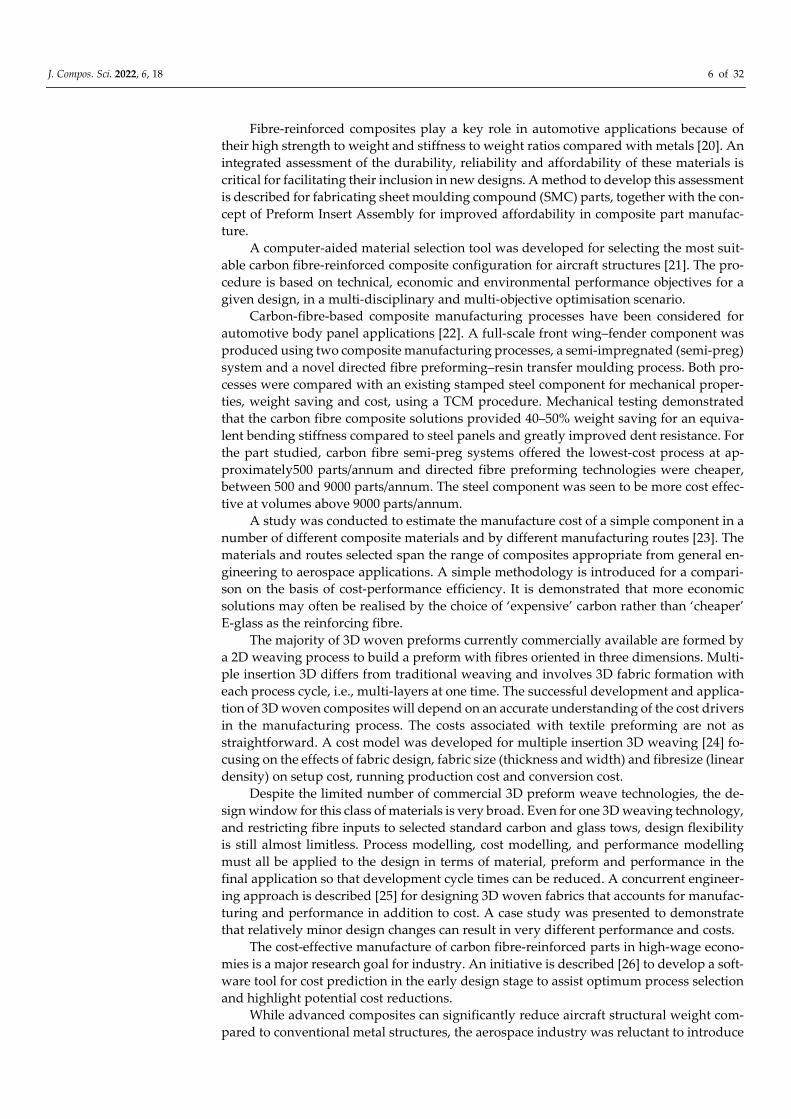
split between loom setup and weaving (Section 3.3). In a Jacquard loom, Figure 3, harness

cords extend down from a control head. Each harness cord is connected to one, two or

sometimes four warp yarns which can be moved individually, allowing for weaving of

much more intricate, complex and longer length 3D fabrics [43]. In the setup phase, fibre

is wound onto bobbins. PTFE tubes glued to an eyeboard will prevent movement of tub-

ing through the eyes and provides fibre tension. The bobbins with wound fibre are then

mounted onto creels followed by fibre being thread through the tubing. Fabric is woven

in a similar fashion to that described for a Weavebird except that each fibre is individually

controlled by the Jacquard head.

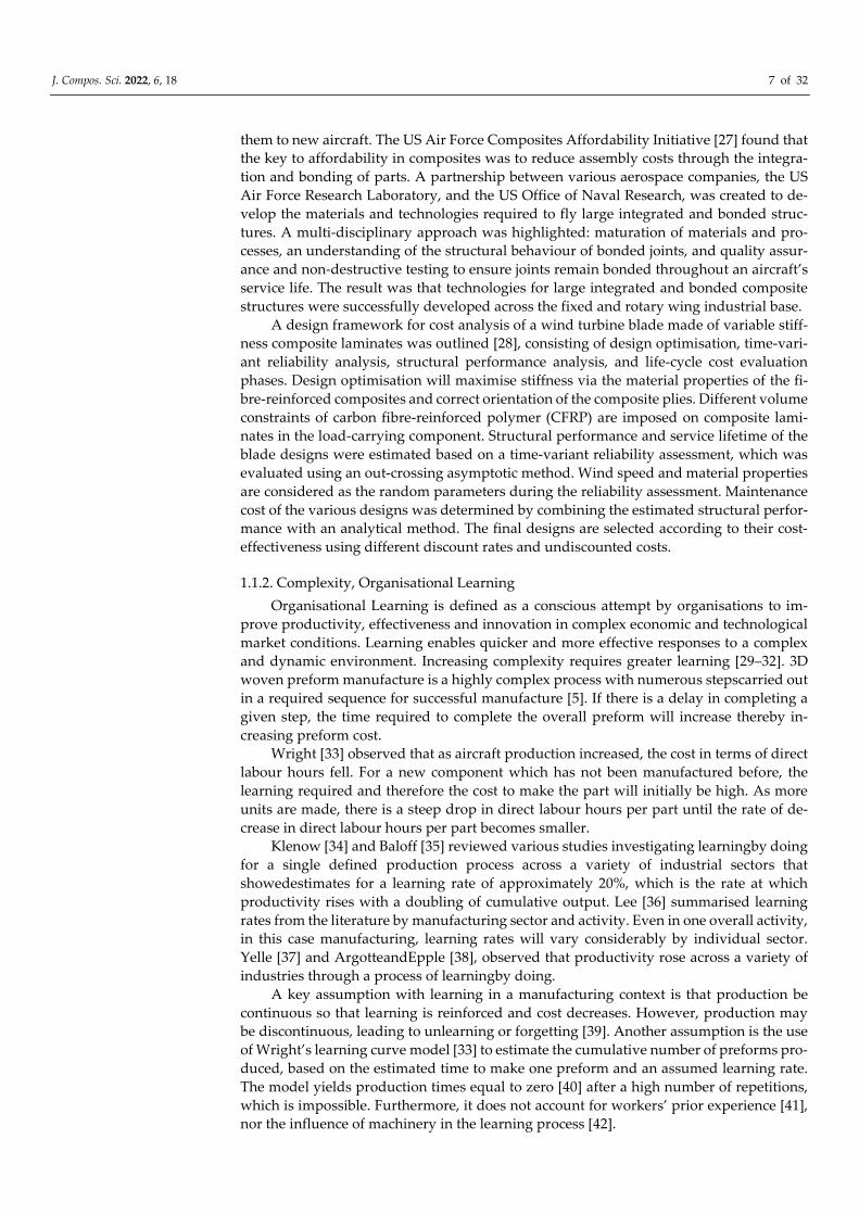
The Weavebird(www.weavebird.com), Figure 4, is a dobby loom. In setup, warp

yarns are taken from a beam mounted on the back of the Weavebird loom and fed though

the eyeboard. The eyeboard controls the warp ends as they enter eyelets on heddles sitting

on loom shafts. The eyeboard houses PTFE tubing which protects the fibre and provides

tension during the weaving process. The heddles are in a sequence determined by the

required architecture. The heddles sit inside shafts or frames, which can lift the warp

threads up or down, one warp thread for each heddle. During weaving, each time a group

of heddles is lifted, a “shed” is created. The shed is the opening between the lifted and

stationary warp threads. The weft is held in a shuttle or rapier, which passes the weft

through the shed to the other side. The shed then closes, and a different set of heddles will

be lifted, creating a new shed, effectively completing the interlacement of warp and weft.

The warp ends are then threaded through the reed, a long, comb-like instrument that

keeps the warp at the correct width and density and helps pack or beat the weft down

into place. Beat up is the motion of weaving that compacts the weft/stuffer yarns with a

consistent force ensuring an even density in the fabric. The woven fabric is wound on the

take-up beam on the front of the loom until the warp on the back beam runs out.

Gurkan [7] notes that while dobby mechanisms work together with harnesses, there

are harness cords for each warp yarn in a Jacquard loom. Therefore, the capability of Jac-

quard looms to make highly complex patterns is the highest among shedding mechanisms

such as dobby, crank or cam.Stewart [43] observed that the main difference between a

dobby and a Jacquard loom is how the warp yarns are moved up and down to form gaps

or sheds through which the weft yarns are drawn by a shuttle to form the weave pattern.

In the case of a dobby loom, the warp yarns can only be controlled in groups moved by

harnesses attached to shafts or frames. When a harness goes up or down, all attached warp

yarns move with the harness. As the loom can only hold a certain number of harnesses,

this means that there is a limit on weave complexity. Dobby looms are best used for mak-

ing simple geometric patterns and short fabric lengths because of harness limitations.

Figure 3. Jacquard loom.

J. Compos. Sci. 2022, 6, 18 9 of 32

Figure 4. Weavebirdloom.

2. Methodology and Experimental

2.1. Methodology

Data for this study came from 17 bespoke 3D woven preforms manufactured by a

Northern Ireland-based company. A resource-based modelling approach was developed

that took account of the bespoke production of each preform utilising the principles that

cost is determined by resources such as material, capital, tooling, energy and labour

(MCTEL), and that cost increases with part complexity. Data for MCTEL resource inputs

were supplied as approximate values for commercial sensitivity reasons. TCM was added

as a further refinement and included a sub-model for how weaving equipment, labour

and energy costs scale with part features such as part shape and complexity.

Dedicated costing for one-off and batch manufacturing

The cost of a 3D fabric preform is the sum of certain cost resources (Equation(1)):

Cost = Material + Tooling Cost + Labour + Overheads (1)

There are two possible production scenarios. In a one-off production scenario, a sin-

gle bespoke part with unique features will be manufactured in a defined time followed by

manufacturing another bespoke part with a different set of unique features in a different

time.In batch production, a given amount of identical parts are manufactured in equal

times.

2.1.1. Costing Methodology for Batch Manufacturing

In batch manufacturing, cost resources for a set of identical parts are defined as fol-

lows.

Material

Material cost for one part of mass m (Equation (2)):

C� = mC� (1 − f)⁄ (2)

where C� is the cost per unit mass of material, m is mass of material, and fis the scrap

rate.

Dedicated Tooling Cost

Dedicated tooling cost Ct for a production run of a part is wholly assigned to the

production run of that part. For a production rate ofn� parts, this cost is written off against

n� and is C� n�⁄ . Tool life n� is the number of parts that a tooling set can make before it

must be replaced. Each time tooling is replaced, there is a step up in the total cost to be

spread over the whole batch. This extra cost is captured by a smoothing factor

(1 + n� n�⁄ )which is multiplied by the tooling cost(Equation (3)):

C� = C� n�⁄ (1 + n� n�⁄ ) (3)

J. Compos. Sci. 2022, 6, 18 10 of 32

Capital Cost

Capital cost Cc is for equipment used to make different parts and associated infra-

structure such as land and buildings. Capital cost is converted into an overhead by a cap-

ital write-off time, two. The resulting quantity, Cc/two is cost per unit time provided equip-

ment and infrastructure are used continuously. Cc/two is divided by a load factor L, the

fraction of time for which the equipment is productive. The contribution of capital to cost

per unit is cost per unit time divided by the production rate n� to give cost per part (Equa-

tion (4)):

C� = 1 n�⁄ (C� Lt��⁄ ) (4)

Labour andUtilities

Overhead Coh is labour, energy, R&D and administration. Dividing by production

rate n� (Equation (5)):

C� = C�� n�⁄ (5)

Therefore, the total manufacturing cost per part C�� is the sum of C1 to C4, or (Equation

(6)):

C�� =mC�

(1 − f)+

C�

n�1 +

n�

n�

� + 1

n�

�C�

Lt��

+ C�� (6)

Note:Equations (1)–(6) are taken from “Materials: Engineering, Science, Processing & De-

sign”[44].

2.1.2. Cost Methodology for One-Off 3D Woven Preform Manufacturing

Cost resources for a unique 3D woven preform are defined as follows.

Material Cost

The material cost for one 3D woven preform of mass m is mCm, and is multiplied by

1/(1 − f) where f is the scrap fraction.

C�� =mC�

(1 − f)

Tooling Cost

Tooling or capital cost Ct is the cost of the weaving loom, creels, bobbins and associ-

ated weaving equipment. This cost is not dedicated to a given preform as the loom can

weave different preforms of varying fibre architectures. Data for other capital costs such

as land and buildings were not provided. Tooling cost is converted into an annual over-

head by dividing by a capital write-off time, two, (e.g., 5 years) over which it is recovered.

The resulting quantity, Cc/two is the annual cost.

C�� =C�

t��

A unique preform will be manufactured in a defined time which will be different

from the time required for another preform. If the annual production time is T hours and

the time taken to make a preform piis t�, the proportion of the annual production time for

this preform is

t�T�

Therefore, the proportion of the annual tooling cost assigned to this preform (Equation

(7)) is:

C�� =t�

T�

C�

t��

� (7)

Labour Cost

J. Compos. Sci. 2022, 6, 18 11 of 32

Labour is the sum of annual salary costs of a weave manager, technician, and other

staff costs:

C�� = � C��

The proportion of the annual labour cost assigned to this preform (Equation (8)) is:

C�� =t�

T� C�� (8)

General Overhead Cost

Finally, general overhead cost is the sum of energy, building rental and administra-

tion costs (Equation (9)):

C�� = � C�� (9)

The proportion of the annual overhead cost assigned to this preform (Equation (10))

is:

C�� =t�

T� C�� (10)

A smoothing factor would be included for a dedicated production run of the same

preform. In this study, individual preforms were manufactured on a one-off basis so that

a smoothing factor would be required to account for the replacement cost of the weave

machine after several production runs for each preform. To simplify the analysis, a

smoothing factor for each preform was not included as only one preform was manufac-

tured at a time.

Therefore, the total manufacturing cost C��for a unique preform pi is the sum of each

cost resource:

C��=

mC�

(1 − f)+

t�

T

C�

Lt��

+t�

T� C�� +

t�

T� C��

Simplifying:

C��=

mC�

(1 − f)+

t�

T�

C�

Lt��

+ � C�� + � C�� (11)

2.1.3. Relationship between Manufacturing Time and Preform Complexity

Preform cost will scale with part complexity [12–14]. Time can be a surrogate for cost,

so preform complexity will scale with preform manufacturing time. Therefore, for a range

of preforms of increasing complexity, manufacturing time, t will increase with increasing

preform complexity, R:

t ∝ R

Time t� is the manufacturing time for the simplest 3D woven preform, called the

baseline preform, and complexity R� is the baseline preform complexity. If t�for a pre-

form p�is expressed relative to t� for the simplest preform and R� is expressed relative

to R�, then:

t�

t�

= m �R�

R�

��

(12)

where m is a constant of proportionality and n is a power factor index assuming a non-

linear relationship betweent and R. As preform complexity R� increases, the time taken

t� to make R� increases compared to a baseline preform R� with time t�. t� t�⁄ is the

relative manufacturing time factor for a preform p�and R� R�⁄ is the relative feature fac-

tor for a preform p�.

J. Compos. Sci. 2022, 6, 18 12 of 32

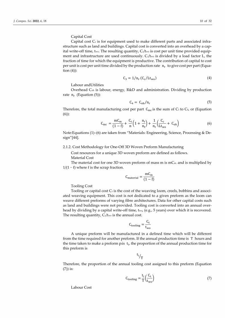
2.1.4. Feature Factor: Quantifying Preform Complexity

Fagade et al. [12–14] define part complexity in terms of features such as the number

of holes, corners, and dimensions. In this study, complexity is a function of the number of

fibre tows (warp andweft) in a preform, and preform shape:

Warp Stuffer—Total number of warp stuffers along the preform width

Weft Filler—Total number of fillers along the preform length

Warp Binder—Total number of through-thickness binders along the width

plus additional sub - featuressuch as the number of holes. For example, a typical 3D pre-

form has a fibre architecture as shown (Figure 5).

Figure 5. Unit cell, orthogonal 3D woven architecture:7 warp layers, 8 weft layers, 28 fibre ends

per unit cell, and 5 warp binder ends.

For given preform p�, the feature factor is assumed to be a function of two overarch-

ing preform features which together make up the preform complexity R�: the total num-

ber of warp stuffers, weft fillers and warp binders A�, and sub-features such as holes and

the sum of preform structural elements ∑ SE� which is a measure of the preform

shape(Equation (13)):

R� = �(A� + sub − features) �� SE�� (13)

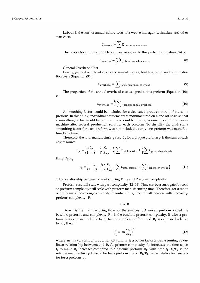
The simplest structural elementis assumed to be a flat profile, Figure 6, and isnum-

bered as 1. Therefore, the number of structural elements reduces to 1 and the baseline

complexity simplifies to:

R� = ∑(A�) (∑ SE�) or R� = ∑(A�) (14)

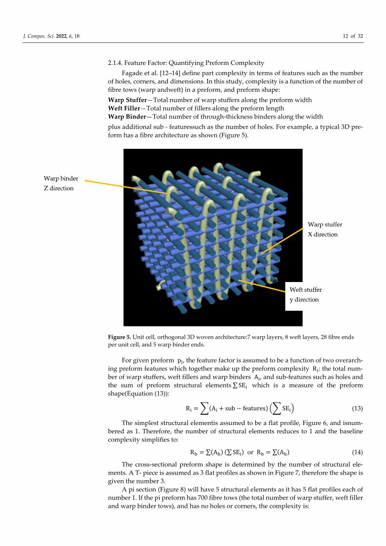
The cross-sectional preform shape is determined by the number of structural ele-

ments. A T- piece is assumed as 3 flat profiles as shown in Figure 7, therefore the shape is

given the number 3.

A pi section (Figure 8) will have 5 structural elements as it has 5 flat profiles each of

number 1. If the pi preform has 700 fibre tows (the total number of warp stuffer, weft filler

and warp binder tows), and has no holes or corners, the complexity is:

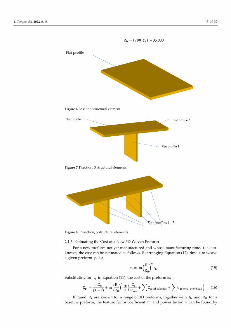
J. Compos. Sci. 2022, 6, 18 13 of 32

R� = (700)(5) = 35,000

Figure 6.Baseline structural element.

Figure 7.T section, 3 structural elements.

Figure 8. Pi section, 5 structural elements.

2.1.5. Estimating the Cost of a New 3D Woven Preform

For a new preform not yet manufactured and whose manufacturing time, t� is un-

known, the cost can be estimated as follows. Rearranging Equation (12), time t�to weave

a given preform p� is:

t� = m �R�

R�

��

t� (15)

Substituting for t� in Equation (11), the cost of the preform is:

C��=

mC�

(1 − f)+ m �

R�

R�

�� t�

T�

C�

Lt��

+ � C�� + � C�� (16)

If t�and R� are known for a range of 3D preforms, together with t� and R� for a

baseline preform, the feature factor coefficient m and power factor n can be found by

J. Compos. Sci. 2022, 6, 18 14 of 32

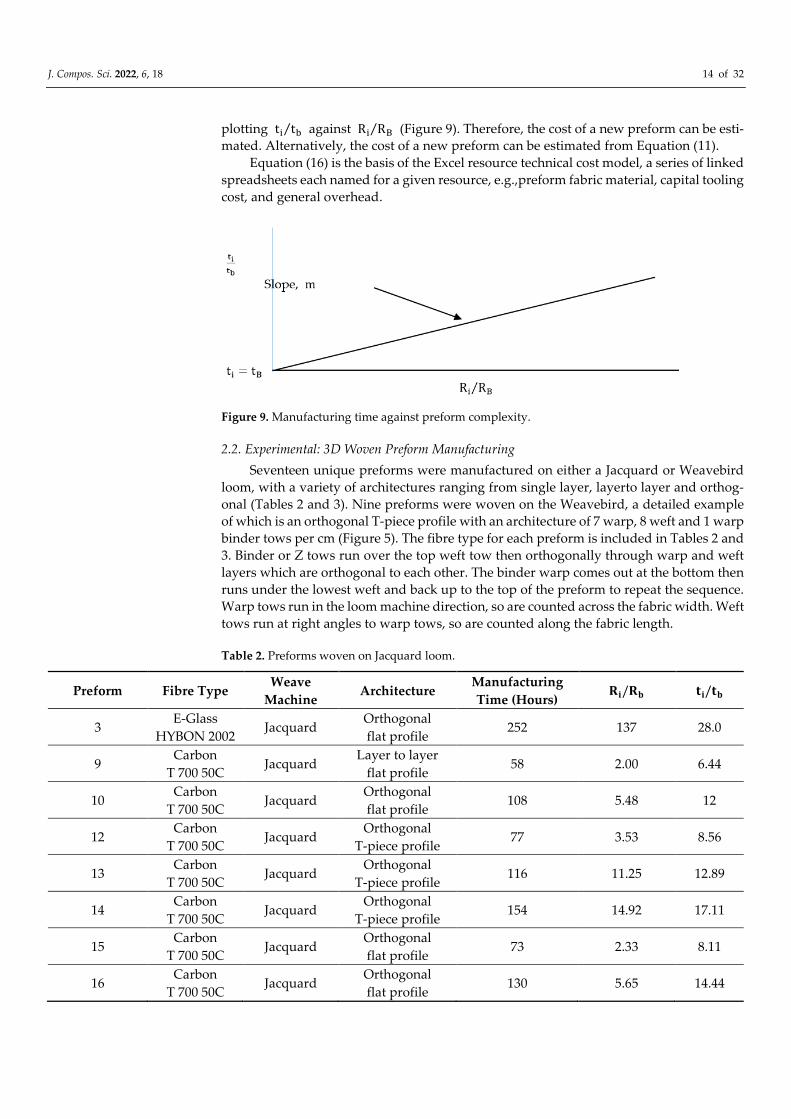
plotting t� t�⁄ against R� R�⁄ (Figure 9). Therefore, the cost of a new preform can be esti-

mated. Alternatively, the cost of a new preform can be estimated from Equation (11).

Equation (16) is the basis of the Excel resource technical cost model, a series of linked

spreadsheets each named for a given resource, e.g.,preform fabric material, capital tooling

cost, and general overhead.

Figure 9. Manufacturing time against preform complexity.

2.2. Experimental: 3D Woven Preform Manufacturing

Seventeen unique preforms were manufactured on either a Jacquard or Weavebird

loom, with a variety of architectures ranging from single layer, layerto layer and orthog-

onal (Tables 2 and 3). Nine preforms were woven on the Weavebird, a detailed example

of which is an orthogonal T-piece profile with an architecture of 7 warp, 8 weft and 1 warp

binder tows per cm (Figure 5). The fibre type for each preform is included in Tables 2 and

3. Binder or Z tows run over the top weft tow then orthogonally through warp and weft

layers which are orthogonal to each other. The binder warp comes out at the bottom then

runs under the lowest weft and back up to the top of the preform to repeat the sequence.

Warp tows run in the loom machine direction, so are counted across the fabric width. Weft

tows run at right angles to warp tows, so are counted along the fabric length.

Table 2. Preforms woven on Jacquard loom.

Preform Fibre Type Weave

Machine Architecture

Manufacturing

Time (Hours) ��/�� /��

3 E-Glass

HYBON 2002 Jacquard

Orthogonal

flat profile 252 137 28.0

9 Carbon

T 700 50C Jacquard

Layer to layer

flat profile 58 2.00 6.44

10 Carbon

T 700 50C Jacquard

Orthogonal

flat profile 108 5.48 12

12 Carbon

T 700 50C Jacquard

Orthogonal

T-piece profile 77 3.53 8.56

13 Carbon

T 700 50C Jacquard

Orthogonal


14 Carbon

T 700 50C Jacquard

Orthogonal


15 Carbon

T 700 50C Jacquard

Orthogonal


16 Carbon

T 700 50C Jacquard

Orthogonal


J. Compos. Sci. 2022, 6, 18 15 of 32

Table 3. Preforms woven on Weavebirdloom.

Preform Fibre Type Weave

Machine Architecture

Manufacturing

Time (Hours) ��/�� /��

1 Carbon

T 700GC Weavebird

Single layer


2 Carbon

T 700GC Weavebird

Layer to layer


4 Carbon T

700GC Weavebird

Orthogonal T-piece

profile 99 11.5 11.0

5 E-Glass

HYBON 2002 Weavebird

Orthogonal T-piece

profile 49 5.18 5.44

6 E-Glass HY-

BON 2002 Weavebird

Orthogonal T-piece

profile 43 5.50 4.78

7 E-Glass HY-

BON 2002 Weavebird

Layer to layer


8 E-Glass HY-

BON 2002 Weavebird

Layer to layer


11 Carbon

T 700 50C Weavebird

Orthogonal


17 Carbon

T700 50C Weavebird

Orthogonal


Table 4 records design and fabric processing step times using Preform 4 as an exam-

ple, the sum of which is the total manufacturing time. The preform was designed on the

Scotweave CAD package and then transferred to the Proweave software package on the

loom, which instructs the loom to weave the preform fabric according to the design archi-

tecture. The total manufacturing time (loom setupandweaving) was itemised as follows

(Table 4).

Table 4. Preform 4 setup and weave manufacturing times.

Stage Loom Setup, Design andWeave Time Required (h)

1 Winding of bobbins 16

2 Bobbins insertion on creel 8

3 Tubing preparation time, 315 tubes 24

4 Passing 315 carbon tows through PTFE

Tubing and loom 24

5 Weave time 3

6 Design on Scotweave 24

Total Manufacturing Time: 99

3. Results

Each preform is unique in terms of complexity. In this study, the key metric for com-

plexity is the product of the total number of fibre tows or warp stuffers, weft fillers and

warp binders, any sub-features such as holes and the sum of preform structural ele-

ments∑ SE�, which is a measure of the preform shape. Complexity is expressed by Equa-

tion (13).

Each preform complexity and manufacturing time is compared to a baseline preform

complexity and manufacturing time, and expressed as the relative feature factor R�/R�

and relative manufacturing time factor t�/t�, respectively. Tables 2 and 3 summarisepre-

forms woven on the Jacquard and Weavebird looms, respectively.

J. Compos. Sci. 2022, 6, 18 16 of 32

3.1. Calculation of�� ⁄ and�� ⁄

The baseline fabric is the simplest in terms of woven architecture compared with the

other fabrics and has the shortest manufacturing time t�. R� is complexity of Preform 1,

(Equation (14)).

As the baseline is a single simple flat profile, ∑ SE� is equal to 1,A� is 360, the total

number of fibre tows. As R� is the same as R�for Preform 1,R� R�⁄ for Preform 1 is 1.

Manufacturing time t� for Preform 1 is 9 h. As t� is the same as t� for Preform 1, t� t�⁄

for Preform 1 is 1. Values of t� t�⁄ andR� R�⁄ were found as follows for Preform 4,which is

a fabric woven in the shape of a T-piece. A T-piece is assumed to be treated as 3 flat profiles

(Figure 7), therefore the shape is given the number 3 or 3 structural elements. For Preform

4, the total number of fibre tows is 1380. Therefore, complexity R� for Preform 4 is:R� =(1380)(3) = 4140 so R�/R� is 4140/360 = 11.5 (Table 3). t� for Preform 4 is 99 h, while t�

is 9 h. Therefore,t� t�⁄ is 99/9 = 11.

Values of t� t�⁄ and R� R�⁄ for the remaining profiles were calculated by the model,

summarised in Tables 2 and 3 and plotted (Figure 10a–c) to validate Equation (12).

3.2. Data Analysis by Loom Type and Preform Architecture

Nine preforms were made on the Weavebird loom, and eight on the Jacquard loom.

Figure 10a has 17 data points, one for each 3D woven preform,and shows a trend of in-

creasing manufacturing time with increasing preform complexity. Each preform varies in

complexity and architecture in terms of the number of weft and warp tows, preform shape

and whether orthogonal or layerto layer. Figure 10a includes Preform 3 which took 252

hours to produce a profile 20 m in length. The complexity value for Preform 3 was 36,901,

the product of the total number of fibre tows (36,901) and one structural element as it is a

flat profile with no extra features such as T sections. Production times for the remaining

preforms ranged from 9 to 130 hours. Correlation coefficient r2 is 0.56.

(a) (b)

y = 3.171x0.520

R² = 0.56

0.000

5.000

10.000

15.000

20.000

25.000

30.000

35.000

40.000

45.000

0 50 100 150

t i/t

b

Ri /Rb

W

J

JJ

W

W

J

W

J

W

W

W

J

W

J

W

ti /tb = 2.5111(RI /RB)0.6717

r² = 0.50.000

2.000

4.000

6.000

8.000

10.000

12.000

14.000

16.000

18.000

20.000

0 10 20

t i/t

b

Ri /Rb

J. Compos. Sci. 2022, 6, 18 17 of 32

(c)

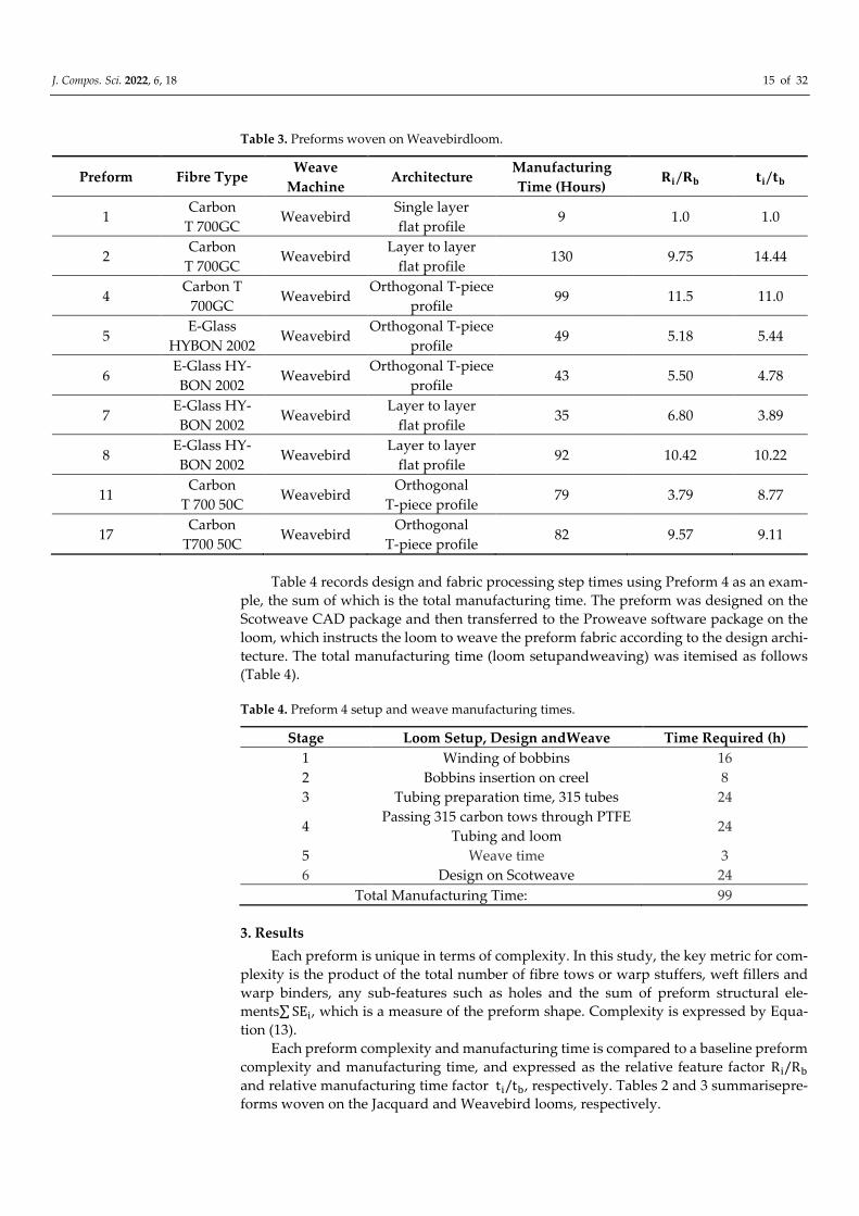
Figure 10. The(a) 17 preforms, (b) 16 preforms, and (c) 14 preforms.

In Figure 10b, Preform3 has been removed. Correlation coefficient r2 is 0.51. Correla-

tion between two variables will either be “weak” [45] or “well related”[46], depending on

sector context. For example, correlation between two variables may be judged either

“weak” in a manufacturing [45] context or “well related” in a public sector context [46].

Two outliers in Figure 10b are due to Preforms 7 and 16. If these are removed, Figure 10c

for 14 profiles gives a significantly improved trend of increasing t� t�⁄ with R� R�⁄ , with

r2 = 0.62 compared with 0.51. Figure 10b,c show a tendency for preforms to separate out

by loom type, with Jacquard preforms tending to group above the trendline and Weave-

bird preforms grouping below. Figure 11a is a plot of nine preforms from the Weavebird

loom. Figure 11b is a plot of eight preforms from the Jacquard loom. Tables 2 (Jacquard)

and 3 (Weavebird) include the weave architecture for each preform.

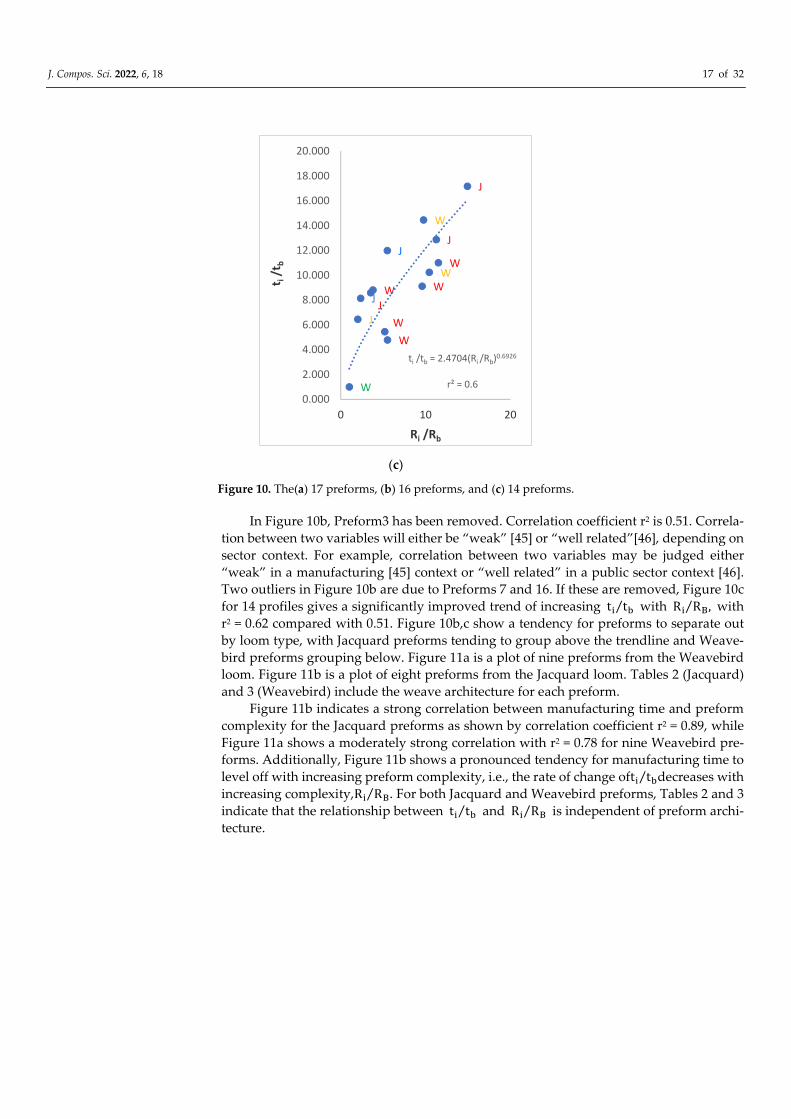
Figure 11b indicates a strong correlation between manufacturing time and preform

complexity for the Jacquard preforms as shown by correlation coefficient r2 = 0.89, while

Figure 11a shows a moderately strong correlation with r2 = 0.78 for nine Weavebird pre-

forms. Additionally, Figure 11b shows a pronounced tendency for manufacturing time to

level off with increasing preform complexity, i.e., the rate of change oft� t�⁄ decreases with

increasing complexity,R� R�⁄ . For both Jacquard and Weavebird preforms, Tables 2 and 3

indicate that the relationship between t� t�⁄ and R� R�⁄ is independent of preform archi-

tecture.

W

J

JJ

W

W

J

W

W

W

J

W

J

W

ti /tb = 2.4704(Ri /Rb)0.6926

r² = 0.6

0.000

2.000

4.000

6.000

8.000

10.000

12.000

14.000

16.000

18.000

20.000

0 10 20

t i/t

b

Ri /Rb

J. Compos. Sci. 2022, 6, 18 18 of 32

(a) (b)

Figure 11. (a)The ninepreforms, Weavebirdloom.(b) The eightpreforms, Jacquard loom.

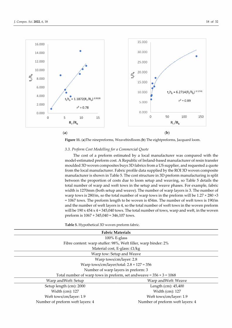
3.3. Preform Cost Modelling for a Commercial Quote

The cost of a preform estimated by a local manufacturer was compared with the

model-estimated preform cost. A Republic of Ireland-based manufacturer of resin transfer

moulded 3D woven composites buys 3D fabrics from a US supplier, and requested a quote

from the local manufacturer. Fabric profile data supplied by the ROI 3D woven composite

manufacturer is shown in Table 5. The cost structure in 3D preform manufacturing is split

between the proportion of costs due to loom setup and weaving, so Table 5 details the

total number of warp and weft tows in the setup and weave phases. For example, fabric

width is 1270mm (both setup and weave). The number of warp layers is 3. The number of

warp tows is 280/m, so the total number of warp tows in the preform will be 1.27 × 280 ×3

= 1067 tows. The preform length to be woven is 454m. The number of weft tows is 190/m

and the number of weft layers is 4, so the total number of weft tows in the woven preform

will be 190 x 454 x 4 = 345,040 tows. The total number of tows, warp and weft, in the woven

preform is 1067 + 345,040 = 346,107 tows.

Table 5. Hypothetical 3D woven preform fabric.

Fabric Materials

100% E-glass

Fibre content: warp stuffer: 98%, Weft filler, warp binder: 2%

Material cost, E-glass: £1/kg

Warp tow: Setup and Weave

Warp tows/cm/layer: 2.8

Warp tows/cm/layer/total: 2.8 × 127 = 356

Number of warp layers in preform: 3

Total number of warp tows in preform, set andweave = 356 × 3 = 1068

Warp andWeft: Setup Warp andWeft: Weave

Setup length (cm): 2000 Length (cm): 45,400

Width (cm): 127 Width (cm): 127

Weft tows/cm/layer: 1.9 Weft tows/cm/layer: 1.9

Number of preform weft layers: 4 Number of preform weft layers: 4

ti/tb = 1.1872(Ri /Rb) 0.9328

r² = 0.78

0.000

2.000

4.000

6.000

8.000

10.000

12.000

14.000

16.000

0 5 10 15

t i/t

b

Ri /Rb

ti/tb = 6.2714(Ri/Rb) 0.3258

r² = 0.89

0.000

5.000

10.000

15.000

20.000

25.000

30.000

35.000

0 50 100 150

t i/t

b

Ri /Rb

J. Compos. Sci. 2022, 6, 18 19 of 32

Weft tows/cm/layer/total: 1.9 × 2000 = 3800 Weft tows/cm/layer/total: 1.9 × 45,400 = 86,260

Weft tows, preform setup: 3800 × 3 = 15,200 Weft tows, weave: 86,260 × 4 = 345,040

Total number of tows: 1068+15,200 = 16,267 Total number of tows: 1067+345,040 = 346,107

Material Cost

Setup fabric area (m2): 1.27 × 20 = 25.4 Weave fabric area (m2): 1.27 × 454.27 = 577

Areal weight (g/m2): 5200 Areal weight (g/m2): 5200

Weight of woven fabric (kg): 5.2 × 25.4 = 132 Weight of woven fabric (kg): 5.2 × 577 = 3000

Cost: £1/kg × 132 = £132 Cost: £1/kg × 3000 = £3000

Total Material Cost: 3000 + 132 = £3132

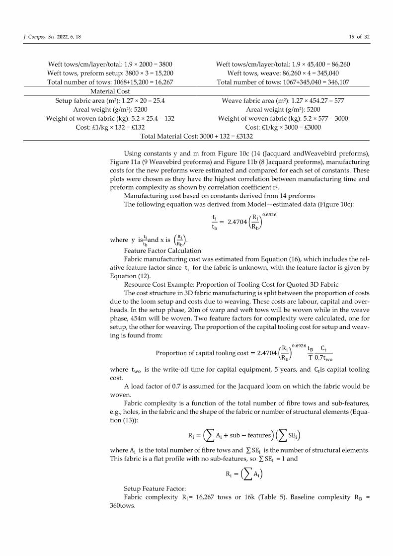
Using constants y and m from Figure 10c (14 (Jacquard andWeavebird preforms),

Figure 11a (9 Weavebird preforms) and Figure 11b (8 Jacquard preforms), manufacturing

costs for the new preforms were estimated and compared for each set of constants. These

plots were chosen as they have the highest correlation between manufacturing time and

preform complexity as shown by correlation coefficient r2.

Manufacturing cost based on constants derived from 14 preforms

The following equation was derived from Model—estimated data (Figure 10c):

t�

t�

= 2.4704 �R�

R�

��.��

where y is��

��and x is �

��

��.

Feature Factor Calculation

Fabric manufacturing cost was estimated from Equation (16), which includes the rel-

ative feature factor since t� for the fabric is unknown, with the feature factor is given by

Equation (12).

Resource Cost Example: Proportion of Tooling Cost for Quoted 3D Fabric

The cost structure in 3D fabric manufacturing is split between the proportion of costs

due to the loom setup and costs due to weaving. These costs are labour, capital and over-

heads. In the setup phase, 20m of warp and weft tows will be woven while in the weave

phase, 454m will be woven. Two feature factors for complexity were calculated, one for

setup, the other for weaving. The proportion of the capital tooling cost for setup and weav-

ing is found from:

Proportion of capital tooling cost = 2.4704 �R�

R�

��.�� t�

T

C�

0.7t��

where t�� is the write-off time for capital equipment, 5 years, and C�is capital tooling

cost.

A load factor of 0.7 is assumed for the Jacquard loom on which the fabric would be

woven.

Fabric complexity is a function of the total number of fibre tows and sub-features,

e.g., holes, in the fabric and the shape of the fabric or number of structural elements (Equa-

tion (13)):

R� = �� A� + sub − features� �� SE��

where A� is the total number of fibre tows and ∑ SE� is the number of structural elements.

This fabric is a flat profile with no sub-features, so ∑ SE� = 1 and

R� = �� A��

Setup Feature Factor:

Fabric complexity R� = 16,267 tows or 16k (Table 5). Baseline complexity R� =

360tows.

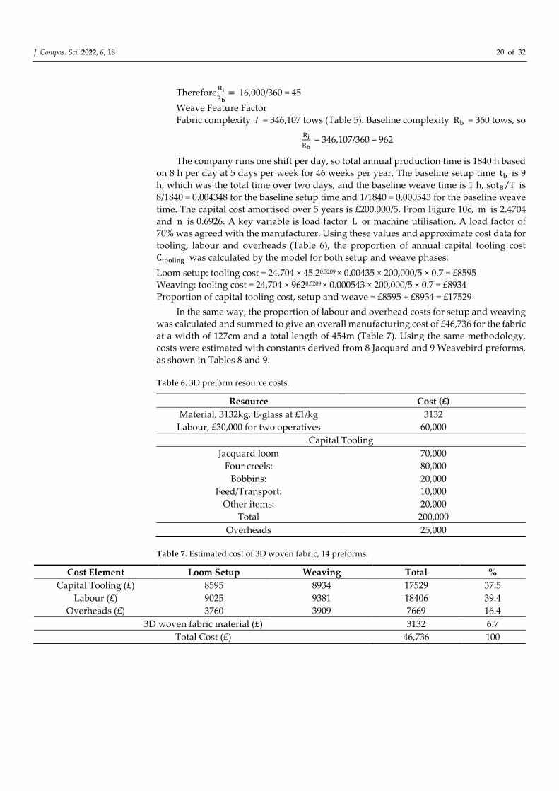
J. Compos. Sci. 2022, 6, 18 20 of 32

Therefore��

��= 16,000/360 = 45

Weave Feature Factor

Fabric complexity � = 346,107 tows (Table 5). Baseline complexity R� = 360 tows, so

��

�� = 346,107/360 = 962

The company runs one shift per day, so total annual production time is 1840 h based

on 8 h per day at 5 days per week for 46 weeks per year. The baseline setup time t� is 9

h, which was the total time over two days, and the baseline weave time is 1 h, sot� T⁄ is

8/1840 = 0.004348 for the baseline setup time and 1/1840 = 0.000543 for the baseline weave

time. The capital cost amortised over 5 years is £200,000/5. From Figure 10c, m is 2.4704

and n is 0.6926. A key variable is load factor L or machine utilisation. A load factor of

70% was agreed with the manufacturer. Using these values and approximate cost data for

tooling, labour and overheads (Table 6), the proportion of annual capital tooling cost

C�� was calculated by the model for both setup and weave phases:

Loom setup: tooling cost = 24,704 × 45.20.5209 × 0.00435 × 200,000/5 × 0.7 = £8595

Weaving: tooling cost = 24,704 × 9620.5209 × 0.000543 × 200,000/5 × 0.7 = £8934

Proportion of capital tooling cost, setup and weave = £8595 + £8934 = £17529

In the same way, the proportion of labour and overhead costs for setup and weaving

was calculated and summed to give an overall manufacturing cost of £46,736 for the fabric

at a width of 127cm and a total length of 454m (Table 7). Using the same methodology,

costs were estimated with constants derived from 8 Jacquard and 9 Weavebird preforms,

as shown in Tables 8 and 9.

Table 6. 3D preform resource costs.

Resource Cost (£)

Material, 3132kg, E-glass at £1/kg 3132

Labour, £30,000 for two operatives 60,000

Capital Tooling

Jacquard loom 70,000

Four creels: 80,000

Bobbins: 20,000

Feed/Transport: 10,000

Other items: 20,000

Total 200,000

Overheads 25,000

Table 7. Estimated cost of 3D woven fabric, 14 preforms.

Cost Element Loom Setup Weaving Total %

Capital Tooling (£) 8595 8934 17529 37.5

Labour (£) 9025 9381 18406 39.4

Overheads (£) 3760 3909 7669 16.4

3D woven fabric material (£) 3132 6.7

Total Cost (£) 46,736 100

J. Compos. Sci. 2022, 6, 18 21 of 32

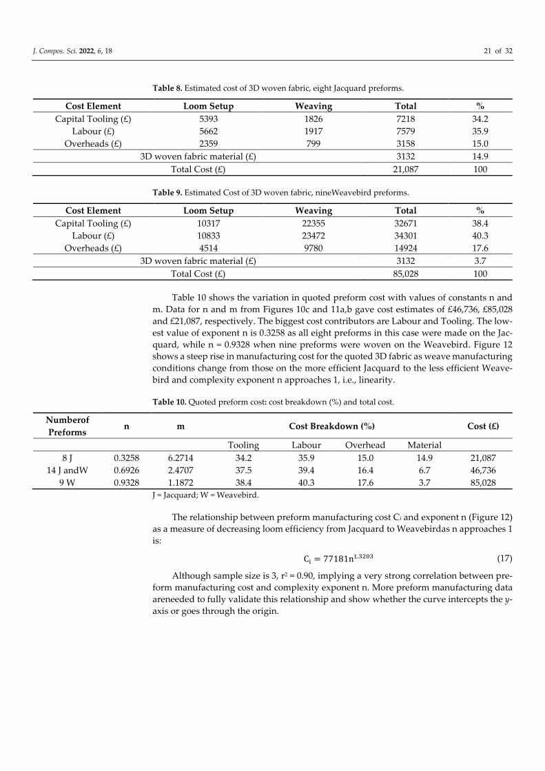
Table 8. Estimated cost of 3D woven fabric, eight Jacquard preforms.


Capital Tooling (£) 5393 1826 7218 34.2

Labour (£) 5662 1917 7579 35.9

Overheads (£) 2359 799 3158 15.0


Total Cost (£) 21,087 100

Table 9. Estimated Cost of 3D woven fabric, nineWeavebird preforms.


Capital Tooling (£) 10317 22355 32671 38.4

Labour (£) 10833 23472 34301 40.3

Overheads (£) 4514 9780 14924 17.6


Total Cost (£) 85,028 100

Table 10 shows the variation in quoted preform cost with values of constants n and

m. Data for n and m from Figures 10c and 11a,b gave cost estimates of £46,736, £85,028

and £21,087, respectively. The biggest cost contributors are Labour and Tooling. The low-

est value of exponent n is 0.3258 as all eight preforms in this case were made on the Jac-

quard, while n = 0.9328 when nine preforms were woven on the Weavebird. Figure 12

shows a steep rise in manufacturing cost for the quoted 3D fabric as weave manufacturing

conditions change from those on the more efficient Jacquard to the less efficient Weave-

bird and complexity exponent n approaches 1, i.e., linearity.

Table 10. Quoted preform cost: cost breakdown (%) and total cost.

Numberof

Preforms n m Cost Breakdown (%) Cost (£)

Tooling Labour Overhead Material

8 J 0.3258 6.2714 34.2 35.9 15.0 14.9 21,087

14 J andW 0.6926 2.4707 37.5 39.4 16.4 6.7 46,736

9 W 0.9328 1.1872 38.4 40.3 17.6 3.7 85,028

J = Jacquard; W = Weavebird.

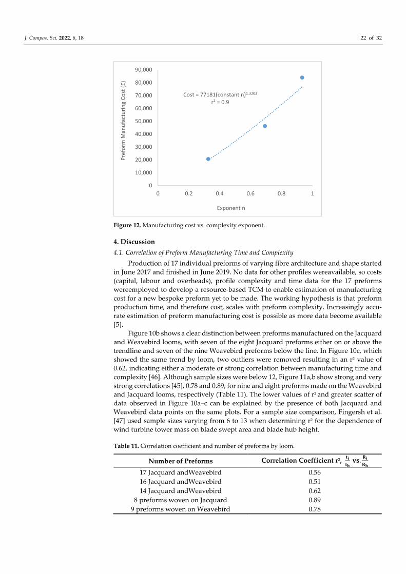
The relationship between preform manufacturing cost Ci and exponent n (Figure 12)

as a measure of decreasing loom efficiency from Jacquard to Weavebirdas n approaches 1

is:

C� = 77181n�.�� (17)

Although sample size is 3, r2 = 0.90, implying a very strong correlation between pre-

form manufacturing cost and complexity exponent n. More preform manufacturing data

areneeded to fully validate this relationship and show whether the curve intercepts the y-

axis or goes through the origin.

J. Compos. Sci. 2022, 6, 18 22 of 32

Figure 12. Manufacturing cost vs. complexity exponent.

4. Discussion

4.1. Correlation of Preform Manufacturing Time and Complexity

Production of 17 individual preforms of varying fibre architecture and shape started

in June 2017 and finished in June 2019. No data for other profiles wereavailable, so costs

(capital, labour and overheads), profile complexity and time data for the 17 preforms

wereemployed to develop a resource-based TCM to enable estimation of manufacturing

cost for a new bespoke preform yet to be made. The working hypothesis is that preform

production time, and therefore cost, scales with preform complexity. Increasingly accu-

rate estimation of preform manufacturing cost is possible as more data become available

[5].

Figure 10b shows a clear distinction between preforms manufactured on the Jacquard

and Weavebird looms, with seven of the eight Jacquard preforms either on or above the

trendline and seven of the nine Weavebird preforms below the line. In Figure 10c, which

showed the same trend by loom, two outliers were removed resulting in an r2 value of

0.62, indicating either a moderate or strong correlation between manufacturing time and

complexity [46]. Although sample sizes were below 12, Figure 11a,b show strong and very

strong correlations [45], 0.78 and 0.89, for nine and eight preforms made on the Weavebird

and Jacquard looms, respectively (Table 11). The lower values of r2 and greater scatter of

data observed in Figure 10a–c can be explained by the presence of both Jacquard and

Weavebird data points on the same plots. For a sample size comparison, Fingersh et al.

[47] used sample sizes varying from 6 to 13 when determining r2 for the dependence of

wind turbine tower mass on blade swept area and blade hub height.

Table 11. Correlation coefficient and number of preforms by loom.

Number of Preforms Correlation Coefficient r2, ��

�� .

��

��

17 Jacquard andWeavebird 0.56



8 preforms woven on Jacquard 0.89

9 preforms woven on Weavebird 0.78

Cost = 77181(constant n)1.3203

r² = 0.9

0

10,000

20,000

30,000

40,000

50,000

60,000

70,000

80,000

90,000

0 0.2 0.4 0.6 0.8 1

Pre

form

Man

ufa

ctu

rin

g C

ost

(£

)

Exponent n

J. Compos. Sci. 2022, 6, 18 23 of 32

Significant variation across all 17 preforms was present according to profile shape

and weave architecture. The Weavebird is suitable for weaving short length profiles while

the Jacquard is suitable for longer preforms such as Preform 3, Table 2. The preforms were

a variety of flat and T-section shapes with weave architecture varying from single layer,

layer to layer and orthogonal. All 17 preforms were woven for the first time with loom

setup issues such as fibre clumping, contact with loom framework and fibre breakage

causing significant time delays. The time recorded for each preformincluded these time

delays (Tables 2 and 3, pp. 16 and 17). In Section 4.3, a reduction in manufacturing time

as learning increases is discussed in detail (Equation (24), p.29, Table 12, p.26).

Jacquard looms can make long complex fabrics much more efficiently than dobby

looms, e.g., the hypothetical fabric (454 m). This is shown clearly in Figure 11b for eight

Jacquard preforms, in which manufacturing time increases at a decreasing rate with com-

plexity and length, i.e., the loom becomes more efficient at weaving longer, more complex

fabrics. Conversely, where all the preforms were made on a Weavebird loom, manufac-

turing time increases almost linearly with complexity, Figure 11a, and weaving efficiency

does not increase with preform complexity.

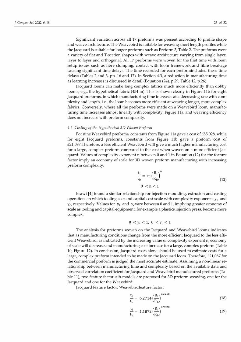
4.2. Costing of the Hypothetical 3D Woven Preform

For nine Weavebird preforms, constants from Figure 11a gave a cost of £85,028, while

for eight Jacquard preforms, constants from Figure 11b gave a preform cost of

£21,087.Therefore, a less efficient Weavebird will give a much higher manufacturing cost

for a large, complex preform compared to the cost when woven on a more efficient Jac-

quard. Values of complexity exponent n between 0 and 1 in Equation (12) for the feature

factor imply an economy of scale for 3D woven preform manufacturing with increasing

preform complexity:

t�

t�

= m �R�

R�

��

0 < n < 1

(12)

Esawi [4] found a similar relationship for injection moulding, extrusion and casting

operations in which tooling cost and capital cost scale with complexity exponents y� and

y�, respectively. Values for y� and y�vary between 0 and 1, implying greater economy of

scale as tooling and capital equipment, for example a plastics injection press, become more

complex:

0 < y� < 1, 0 < y� < 1

The analysis for preforms woven on the Jacquard and Weavebird looms indicates

that as manufacturing conditions change from the more efficient Jacquard to the less effi-

cient Weavebird, as indicated by the increasing value of complexity exponent n, economy

of scale will decrease and manufacturing cost increase for a large, complex preform (Table

10, Figure 12). In conclusion, Jacquard costs alone should be used to estimate costs for a

large, complex preform intended to be made on the Jacquard loom. Therefore, £21,087 for

the commercial preform is judged the most accurate estimate. Assuming a non-linear re-

lationship between manufacturing time and complexity based on the available data and

observed correlation coefficient for Jacquard and Weavebird manufactured preforms (Ta-

ble 11), two feature factor sub-models are proposed for 3D preform weaving, one for the

Jacquard and one for the Weavebird:

Jacquard feature factor: Weavebirdfeature factor:

t�

t�

= 6.2714 �R�

R�

��.��

(18)

t�

t�

= 1.1872 �R�

R�

��.��

(19)

J. Compos. Sci. 2022, 6, 18 24 of 32

which in turn leads to two cost models for preform manufacturing cost, C�:

Jacquard cost model

C� =mC�

(1 − f)+ 6.27 �

R�

R�

��.�� t�

T�

C�

Lt��

+ � C�� + � C�� (20)

Weavebirdcost model

C� =mC�

(1 − f)+ 1.19 �

R�

R�

��.�� t�

T�

C�

Lt��

+ � C�� + � C�� (21)

The cost estimate of £21,087 is approximately three times that for the same preform

supplied by a US manufacturer, or £7500. The lower cost may be due to a higher produc-

tion rate coupled with a more efficient loom leading to lower preform cost and greater

experience from embedded learning.

4.3. Cost Reduction by Learning

Organisational Learning is defined as a conscious attempt by organisations to im-

prove productivity, effectiveness and innovation in complex economic and technological

market conditions. Learning enables quicker and more effective responses to a complex

and dynamic environment. The greater the complexity, the greater the need for learning

[29–32]. 3D woven preform manufacture is a highly complex process with numerous step-

scarried out in a required sequence for successful manufacture. If there is a delay in com-

pleting agiven step, the time required to complete the overall preform will increase

thereby increasing preform cost. In this study, 17 preforms were made for the first time

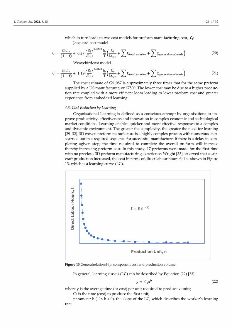
with no previous 3D preform manufacturing experience. Wright [33] observed that as air-

craft production increased, the cost in terms of direct labour hours fell as shown in Figure

13, which is a learning curve (LC).

Figure 13.Generalrelationship, component cost and production volume.

In general, learning curves (LC) can be described by Equation (22) [33]:

y = C�x� (22)

where y is the average time (or cost) per unit required to produce x units;

C1 is the time (cost) to produce the first unit;

parameter b (−1< b < 0), the slope of the LC, which describes the worker’s learning

rate.

t = Kn - C

Dir

ect

Lab

ou

r H

ou

rs, t

Production Unit, n

J. Compos. Sci. 2022, 6, 18 25 of 32

For a new component not previously manufactured, the learning required and there-

fore the cost to make the part will initially be high as shown by the start of the slope on

the left of Figure 11. As more units are made, there is a steep drop in labour hours per part

until the rate of decrease in direct labour hours per part becomes smaller.

Klenow [34] reviewed various studies investigating learning by doing for a single

defined production process across a variety of industrial sectors, observing estimates of

approximately 20% for the learning rate. Baloff [35], and Garg and Milliman [48] showed

that 20% is the rate at which productivity rises with a doubling of cumulative output. Lee

[36] summarised learning rates by manufacturing sector and activity (Table 12) and

showed that even in one overall activity, in this case industrial manufacturing, learning

rates will vary considerably by individual sector. In several studies, Yelle [37] and Argotte

and Epple [38], observed that productivity rose across a variety of industries through a

process of learning by doing.

Table 12. Representative learning rates by industrial sector.

Sector Representative Learning Rates

Aerospace 15%

Shipbuilding 15%–20%

Machine Tools (new models) 15%–20%

Electronics (repetitive) 5%–10%

Electrical Wiring (repetitive) 15%–25%

Machining 5%–10%

75% Manual Assembly + 25% Machining 20%



Punch Press 5%–10%

Raw Materials 5%–7%

Purchased Parts 12%–15%

Welding (repetitive) 10%

In preform manufacture, direct labour hours are associated with activities such as

bobbin winding and insertion, tube preparation time, loom maintenance and operation,

and stoppage time due to issues encountered during weaving, e.g., damage to carbon and

glass fibres from contact with the loom framework. Manufacturing time in this study is

the time taken to complete these activities. With increased preform production, manufac-

turing time t� and manufacturingcost should decrease with increased learning. The esti-

mated manufacturing timet� for one preform is found from Equation (12),

t�

t�

= m �R�

R�

��

from which

t� = m �R�

R�

��

t�

3D fabric manufacturing cost is split between the proportion of costs due to loom

setup and costs due to weaving, therefore there are two manufacturing times for a given

preform: t� �� and t� ��. The estimated cost of the commercial preform was £21,087

(Table 10) for weaving on the Jacquard loom. The company has no experience of making

this preform. Setup time and weave time t� for the baseline preform was 8 and 1 h, re-

spectively. Using values for constants m and n (Table 10), the estimated setup and

weave times for the hypothetical preform are:

Setup time: t� �� = 6.2714(45.19)�.�� 8 = 174 h

J. Compos. Sci. 2022, 6, 18 26 of 32

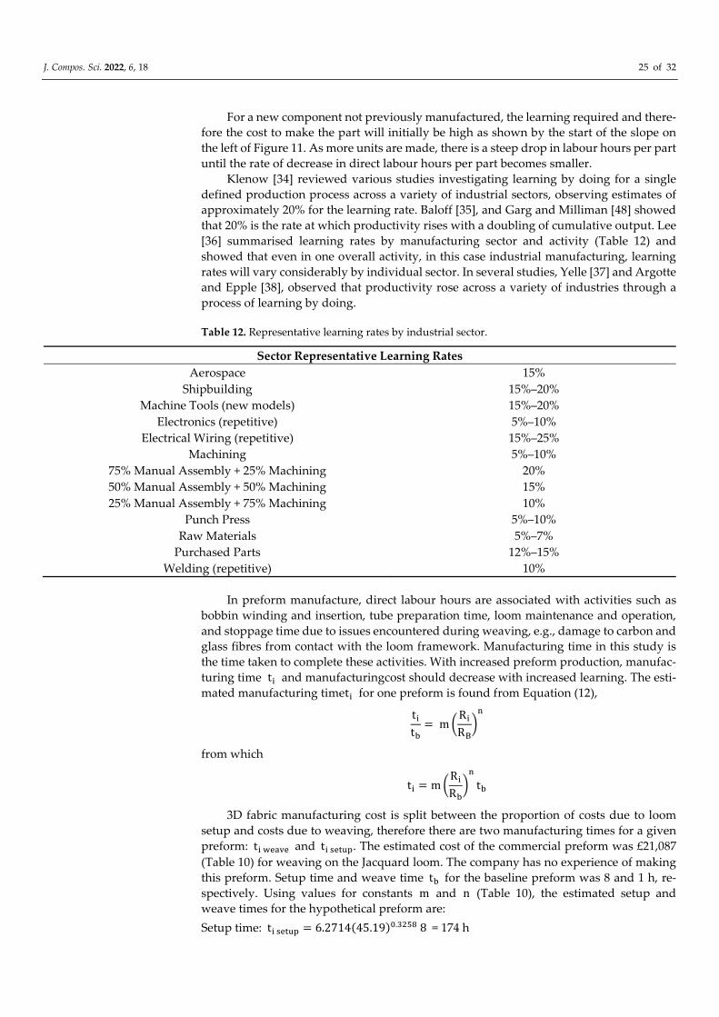
Weave time: t� �� = 6.2714(962)�.�� 1 = 59 h

Total manufacturing time: t� �� + It� �� = 174 + 59 = 233 h

No data werepublicly available for 3D preform learning rates. The total estimated

manufacturing time is 233 h. Setup time is the manual labour time involved in activities

such as bobbin winding, bobbin placement on the creel and taking fibre tow onto the

loom. The setup time is 174/233 or 74.7% while the weave or machine time is 25.3%. From

Table 12, a learning rate of 20%, in which manufacturing time decreases by 20% for each

doubling of cumulative production, corresponds to a manufacturing activity in which

manual operations are 75% and machine time is 25% of total activity. Since manual setup

time (74.7%) and weave time (25.3%) are closest to 75% manual assembly and 25% ma-

chining, 20% was the assumed learning rate for the new preform. Based on this rate, a

learning curve (Figure 14) and an equation (Equation (23)) was derived by the model from

Equation (22), to estimate a competitive manufacturing cost for the new preform.

Figure 14. Learning curve for commercial preform i.

t� = 233b��.�� (23)

where t� = preform manufacturing time;b = number of preforms.

The model estimated a manufacturing time t� of 98 h per preform after a cumulative

production of 15 preforms. Therefore, setup time and weave time will have decreased

with increased cumulative production. Insertion of this value for t� in Equation (11) to-

gether with resource costs for tooling, salaries, overhead, write-off time (Table 6) and load

factor 0.7 gave an estimated cost of £8002,approximately one third of the first-time pre-

form cost of £21,087 and in line with the US supplier’s cost of £7500. More manufacturing

data will be required to clarify learning rates for 3D woven preforms to fully validate

Equation (23) and provide a more accurate estimate of preform cost.

C��=

mC�

(1 − f)+

t�

T�

C�

Lt��

+ � C�� + � C�� (11)

= 3132 +98

1840�200,000

0.7 × 5� + 60000 + 25000� = £8002

Various issues were encountered during first-time preform manufacture:

Fibre catching on the edges of the bobbin.

ti = 233n - 0.32

0

50

100

150

200

250

0 100 200 300 400 500 600 700 800 900

Tim

e, t

per

pre

form

i(h

ou

rs)

Number of preforms, b

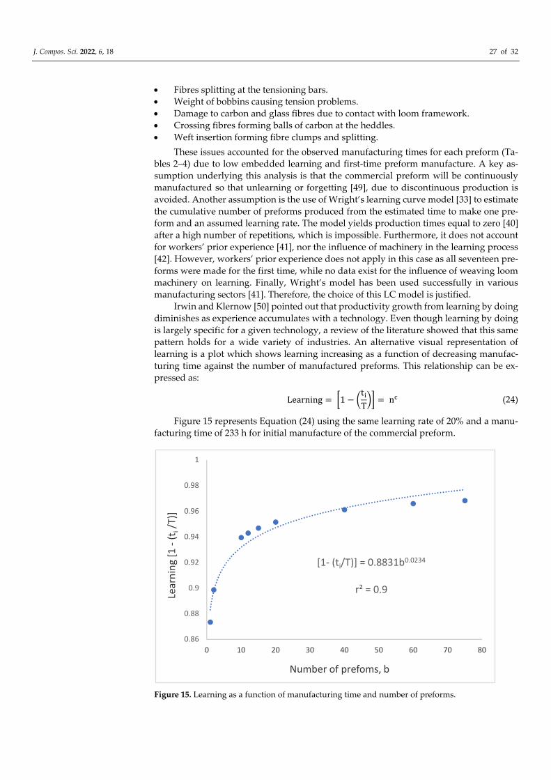
J. Compos. Sci. 2022, 6, 18 27 of 32

Fibres splitting at the tensioning bars.

Weight of bobbins causing tension problems.

Damage to carbon and glass fibres due to contact with loom framework.

Crossing fibres forming balls of carbon at the heddles.

Weft insertion forming fibre clumps and splitting.

These issues accounted for the observed manufacturing times for each preform (Ta-

bles 2–4) due to low embedded learning and first-time preform manufacture. A key as-

sumption underlying this analysis is that the commercial preform will be continuously

manufactured so that unlearning or forgetting [49], due to discontinuous production is

avoided. Another assumption is the use of Wright’s learning curve model [33] to estimate

the cumulative number of preforms produced from the estimated time to make one pre-

form and an assumed learning rate. The model yields production times equal to zero [40]

after a high number of repetitions, which is impossible. Furthermore, it does not account

for workers’ prior experience [41], nor the influence of machinery in the learning process

[42]. However, workers’ prior experience does not apply in this case as all seventeen pre-

forms were made for the first time, while no data exist for the influence of weaving loom

machinery on learning. Finally, Wright’s model has been used successfully in various

manufacturing sectors [41]. Therefore, the choice of this LC model is justified.

Irwin and Klernow [50] pointed out that productivity growth from learning by doing

diminishes as experience accumulates with a technology. Even though learning by doing

is largely specific for a given technology, a review of the literature showed that this same

pattern holds for a wide variety of industries. An alternative visual representation of

learning is a plot which shows learning increasing as a function of decreasing manufac-

turing time against the number of manufactured preforms. This relationship can be ex-

pressed as:

Learning = �1 − �t�

T�� = n� (24)

Figure 15 represents Equation (24) using the same learning rate of 20% and a manu-

facturing time of 233 h for initial manufacture of the commercial preform.

Figure 15. Learning as a function of manufacturing time and number of preforms.

[1- (ti/T)] = 0.8831b0.0234

r² = 0.9

0.86

0.88

0.9

0.92

0.94

0.96

0.98

1

0 10 20 30 40 50 60 70 80

Lear

nin

g [1

-(t

i/T

)]

Number of prefoms, b

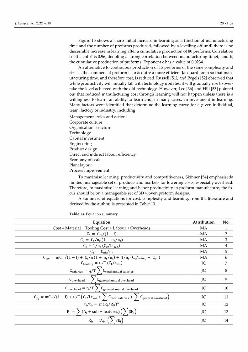
J. Compos. Sci. 2022, 6, 18 28 of 32

Figure 15 shows a sharp initial increase in learning as a function of manufacturing

time and the number of preforms produced, followed by a levelling off until there is no

discernible increase in learning after a cumulative production of 80 preforms. Correlation

coefficient r2 is 0.96, denoting a strong correlation between manufacturing timet� and b,

the cumulative production of preforms. Exponent c has a value of 0.0234.

An alternative to continuous production of 15 preforms of the same complexity and

size as the commercial preform is to acquire a more efficient Jacquard loom so that man-

ufacturing time, and therefore cost, is reduced. Russell [51], and Pegels [52] observed that

while productivity will initially fall with technology updates, it will gradually rise to over-

take the level achieved with the old technology. However, Lee [36] and Hill [53] pointed

out that reduced manufacturing cost through learning will not happen unless there is a

willingness to learn, an ability to learn and, in many cases, an investment in learning.

Many factors were identified that determine the learning curve for a given individual,

team, factory or industry, including

Management styles and actions

Corporate culture

Organisation structure

Technology

Capital investment

Engineering

Product design

Direct and indirect labour efficiency

Economy of scale

Plant layout

Process improvement

To maximise learning, productivity and competitiveness, Skinner [54] emphasiseda

limited, manageable set of products and markets for lowering costs, especially overhead.

Therefore, to maximise learning and hence productivity in preform manufacture, the fo-

cus should be on a manageable set of 3D woven preform designs.

A summary of equations for cost, complexity and learning, from the literature and

derived by the author, is presented in Table 13.

Table 13. Equation summary.

Equation Attribution No.

Cost = Material + Tooling Cost + Labour + Overheads MA 1

C� = C� (1 − f)⁄ MA 2

C� = C� n�⁄ (1 + n� n�⁄ ) MA 3

C� = 1 n�⁄ (C� Lt��⁄ ) MA 4

C� = C�� n�⁄ MA 5

C�� = mC� (1 − f)⁄ + C� n⁄ (1 + n� n�⁄ ) + 1 n�⁄ (C� Lt��⁄ + C��) MA 6

C�� = t� T⁄ (C� t��⁄ ) JC 7

C�� = t� T⁄ � C�� JC 8

C�� = � C�� JC 9

C�� = t� T⁄ � C�� JC 10

C��= mC� (1 − f)⁄ + t� T⁄ �C� Lt��⁄ + � C�� + � C�� JC 11

t� t�⁄ = m(R� R�⁄ )� JC 12

R� = �(A� + sub − features) �� SE�� JC 13

R� = (A�) �� SE�� JC 14

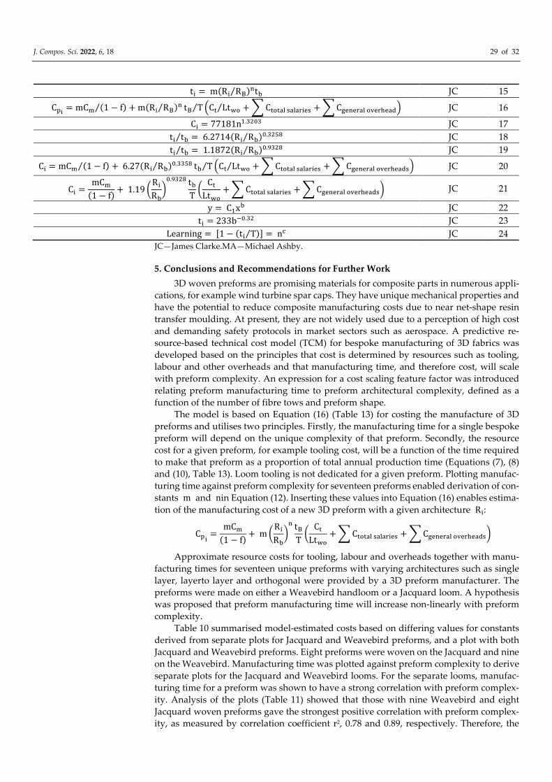
J. Compos. Sci. 2022, 6, 18 29 of 32

t� = m(R� R�⁄ )�t� JC 15

C��= mC� (1 − f)⁄ + m(R� R�⁄ )� t� T⁄ �C� Lt��⁄ + � C�� + � C�� JC 16

C� = 77181n�.�� JC 17

t� t�⁄ = 6.2714(R� R�⁄ )�.�� JC 18

t� t�⁄ = 1.1872(R� R�⁄ )�.�� JC 19

C� = mC� (1 − f)⁄ + 6.27(R� R�⁄ )�.�� t� T⁄ �C� Lt��⁄ + � C�� + � C�� JC 20

C� =mC�

(1 − f)+ 1.19 �

R�

R�

��.�� t�

T�

C�

Lt��

+ � C�� + � C�� JC 21

y = C�x� JC 22

t� = 233b��.�� JC 23

Learning = [1 − (t� T⁄ )] = n� JC 24

JC—James Clarke.MA—Michael Ashby.

5. Conclusions and Recommendations for Further Work

3D woven preforms are promising materials for composite parts in numerous appli-

cations, for example wind turbine spar caps. They have unique mechanical properties and

have the potential to reduce composite manufacturing costs due to near net-shape resin

transfer moulding. At present, they are not widely used due to a perception of high cost

and demanding safety protocols in market sectors such as aerospace. A predictive re-

source-based technical cost model (TCM) for bespoke manufacturing of 3D fabrics was

developed based on the principles that cost is determined by resources such as tooling,

labour and other overheads and that manufacturing time, and therefore cost, will scale

with preform complexity. An expression for a cost scaling feature factor was introduced

relating preform manufacturing time to preform architectural complexity, defined as a

function of the number of fibre tows and preform shape.

The model is based on Equation (16) (Table 13) for costing the manufacture of 3D

preforms and utilises two principles. Firstly, the manufacturing time for a single bespoke

preform will depend on the unique complexity of that preform. Secondly, the resource

cost for a given preform, for example tooling cost, will be a function of the time required

to make that preform as a proportion of total annual production time (Equations (7), (8)

and (10), Table 13). Loom tooling is not dedicated for a given preform. Plotting manufac-

turing time against preform complexity for seventeen preforms enabled derivation of con-

stants m and nin Equation (12). Inserting these values into Equation (16) enables estima-

tion of the manufacturing cost of a new 3D preform with a given architecture R�:

C��=

mC�

(1 − f)+ m �

R�

R�

�� t�

T�

C�

Lt��

+ � C�� + � C��

Approximate resource costs for tooling, labour and overheads together with manu-

facturing times for seventeen unique preforms with varying architectures such as single

layer, layerto layer and orthogonal were provided by a 3D preform manufacturer. The

preforms were made on either a Weavebird handloom or a Jacquard loom. A hypothesis

was proposed that preform manufacturing time will increase non-linearly with preform

complexity.

Table 10 summarised model-estimated costs based on differing values for constants

derived from separate plots for Jacquard and Weavebird preforms, and a plot with both

Jacquard and Weavebird preforms. Eight preforms were woven on the Jacquard and nine

on the Weavebird. Manufacturing time was plotted against preform complexity to derive

separate plots for the Jacquard and Weavebird looms. For the separate looms, manufac-

turing time for a preform was shown to have a strong correlation with preform complex-

ity. Analysis of the plots (Table 11) showed that those with nine Weavebird and eight

Jacquard woven preforms gave the strongest positive correlation with preform complex-

ity, as measured by correlation coefficient r2, 0.78 and 0.89, respectively. Therefore, the

J. Compos. Sci. 2022, 6, 18 30 of 32

hypothesis of preform manufacturing time increasing non-linearly with preform com-

plexity is considered valid based on the cost information and preform data provided.

More data from a wider range of preforms of varying complexity arerequired to fully val-

idate the non-linear relationship between manufacturing time and complexity.

A composite parts manufacturer received a quote for a single large, complex preform

currently made by a US manufacturer for £7500. The cost of the new preform was com-

pared with cost estimates for the preform based on data from preforms made on either

the Jacquard or Weavebird looms. Analysis of the plots showed that the Jacquard weaves

large, complex preforms more efficiently than the Weavebird. Therefore, the estimated

cost for the preform, £21,087 based on data derived from the plot for eight Jacquardwoven

preforms, was judged the most realistic although almost three times that of the US-sup-

plier’s cost of £7500. Based on a weight of 3132kg, the cost per kg for the US fabric is

£2.4/kg. The raw fibre (E-glass) cost is £1/kg, so the material cost proportion for the fabric

is 42%. For one-off preform manufacture, the material cost proportion varied from 3.7%

to 4.9%, depending on whether the preform is to be made on a Weavebird or Jacquard

loom. A recent cost modelling study of mass-produced wind turbine spar caps made with

glass fibre composite {5} showed material proportions ranging from 35% to 52%, similar

to a cost proportion of 42%, implying that the US-supplied fabric has been similarly mass

produced, resulting in a cost per preform of £7500 compared to a one-off manufacturing

cost of £21,087. A learning curve was derived based on a learning rate from the estimated

labour and machine time proportions of total preform manufacturing time. From the

learning curve, continuous production of 15 preforms resulted in a cost per preform of

£8001, assuming no reduction in other costs such astooling and infrastructure.

In concluding, the results imply that it is possible to make unique 3D woven preforms

competitively on a suitable loom machine, provided that sufficient learning is embedded

in the manufacturing organisation coupled with greater automation. Although studies

have indicated that cost per part will initially increase following machine installation, cost

per part will fall below the level present before machine installation as new learning is

embedded for successful machine operation. This should encourage increased uptake of

suitably designed 3D woven composites in a wider range of applications.

Further work could investigate mass customisation, where short manufacturing runs

for a part of given size and complexity are coupled with fast turnaround times and tool

changes for another part. This can be very expensive owing to a lack of embedded learning

in a fast-changing production environment. Short runs of bespoke 3D woven preforms

could be modelled more accurately if extensions of traditional learning curve models in-

corporating multi-variate analysis can be developed. Multi-variate learning curves are

based on two or more independent variables and are required when quantitative and

qualitative factors run in tandem, e.g., when fast tool changes are required for a run of

new preforms. To date, development of multi-variate analysis tools for constantly chang-

ing scenarios has been sparse, a key issue being lack of real time manufacturing process

data. However, recent advances in digital twin technology enabling real time imaging of

a manufacturing operation based on worker performance and process data should en-

courage the development of multi-variate learning curves for improving worker learning

so that the cost of short production runs of 3D woven preforms is reduced.

Author Contributions: Conceptualisation, J.C.; data curation, J.C.; formal analysis, J.C.; investiga-

tion, J.C.; methodology, J.C.; project administration, A.M. and E.A.; resources, A.M. and E.A.; soft-

ware, J.C.; validation, G.S. and R.B.; visualisation, J.C.; writing—original draft, J.C.; writing—review

andediting, J.C., A.M., J.S.,and D.D. All authors have read and agreed to the published version of

the manuscript.

Funding: This research received no external funding.

Acknowledgments: The author would like to thankTomas Flanagan or Eire Composites for provid-

ing valuable advice and guidance in cost modelling for wind turbine spar cap manufacture.

J. Compos. Sci. 2022, 6, 18 31 of 32

Conflicts of Interest: The authors declare no conflict of interest.

References

1. The Aerospace Composites Market, 2012–2022. 2012. Available online: www.visiongain.com(accessed on 20.9.2019.

2. O’Dea, N. Global Outlook for the Composites Industry, Presentation, Advanced Engineering, Composites Forum; NEC: Birmingham,

UK, 2018.

3. Stig, F.; Hallström, S. Assessment of the mechanical properties of a new 3D woven fibre composite material. Compos. Sci. Technol.

2009, 69, 1686–1692.

4. Esawi, A.M.K.; Ashby M.F. Cost estimates to guide pre-selection of processes. Mater. Des. 2003, 24, 605–616.

5. Clarke, J. A Cost Model Framework for 3D Woven Composites. Ph.D. Thesis, Ulster University, Belfast, UK, 2020.

6. Boussu, F.; Cristian, I.; Neumann, S. Generaldefinition of 3D warp interlock fabric architecture. Compos. Part B Eng.2015, 81,

171–188.

7. Gurkan, P.; Namak, U. 3D Woven Fabrics. Woven Fabrics 2012, 4, 91–120.

8. Van Mourik, A. Why Conversion Costs of Composites in Aerospace are Still Way too High. LinkedIn Arti-

cle.https://www.linkedin.com/pulse/why-conversion-costs-composites-aerospace-still-way-too-mourik-van/16 July 2018. Ac-

cessed on 20.9.2019.

9. McClain, M.; Goering, J. Rapid assembly of fiber preforms using 3D wovencomponents. Sampe J. 2013, 49, 24–31.

10. Mohamed, M.; Wetzel, K. 3D Woven Carbon/Glass Hybrid Spar Cap for Wind Turbine Rotor Blade. J. Sol. Energy Eng. 2006,

128, 562–573.

11. Hueber, K.;R.Schledjewski. Review of cost estimation: Methods and models for aerospace composite manufacturing. Adv.

Manuf. Polym. Compos. Sci. 2016, 2, 1–13.

12. Fagade, A.A.; Kazmer, D.O. Early cost estimation for injection moldedparts. J. Inject. Molding Technol.2000, 3, 97–106.

13. Fagade, A.A.; Kazmer, D.O. Modelling the effects of complexity on manufacturing costsand time-to-market of plastic injection

molded products. In Proceedings of the Tenth Annual Conference of the Production and Operations Management Society, POM

99, Charleston, SC, USA, 20–23 March 1999.

14. Fagade, A.; Kazmer, D.; Kapoor, D. A Discussion of Design and Manufacturing Complexity;Department of Mechanical and Indus-

trial Engineering, University of Massachusetts: Amherst, MA 01003, USA. 2000.Available online: http://citese-

erx.ist.psu.edu/viewdoc/download?doi=10.1.1.495.2899&rep=rep1&type=p(accessed on 20.9.2019).

15. Hagnell, M.K.; Akermo, M.A Composite Cost Model for the Aeronautical Industry: Methodology and Case Study. Compos. Part

B Eng. 2015,79, 254–261.

16. Gutowski, T.G.; Neoh, E.T.; Polgar, K.C. Adaptive Framework for Fabrication Time of Advanced Composite Manufacturing Processes;

Technical Report; Laboratory for Manufacturing and Productivity, Massachusetts Institute of Technology: Cambridge, MA,

USA, 1995.

17. Verrey, J.; Wakeman, M.D.; Michaud, V.; Manson, J.A.E. Manufacturing Cost Comparison of Thermoplastic and Thermoset RTM for

an Automotive Floor Pan; EcolePolytechniqueFe´de´rale de Lausanne (EPFL), Laboratoire de Technologie des Composites et-

Polyme’res (LTC): Lausanne, Switzerland, 2005.

18. Schubel, P. Cost Modelling in polymer composite applications. Case study:Analysis of existing and automated manufacturing

processes for a large windturbine blade. Compos. Part B 2012, 43, 953–960.

19. Ennis, B.L.; Kelley, C.L.; Naughton, B.T.; Norris, R.E.; Das, S.; Lee, D.; Miller, D.A. Optimized Carbon Fibre Composite in a Wind

Turbine Blade Design; Sandia Report, SAND 2019-14173; Sandia National Laboratories: Albuquerque, NM, USA, 2019.

20. Cabrera-Ríos, M.; Castro, J.M. The balance between durability, reliability and affordability in structural composites manufac-

turing. Polym. Compos.2007, 28, 233–240.

21. Calado, E.; Leite, M.; Silva, A. Selecting composite materials considering cost and environmental impact in the early phases of

aircraft structure design. J. Clean. Prod.2018, 186, 113–122.

22. Turner, T.; Harper, L.; Warrior, N.; Rudd, C. Low-cost carbon-fibre-based automotive body panel systems: A performance and

manufacturing cost comparison, Proc. Inst. Mech. Eng. Part D J. Automob. Eng.2008, 222, 53–63.

23. Bader, M. Selection of composite materials and manufacturing routes for cost-effective performance. Compos. Part A Appl. Sci.

Manuf.2002, 33, 913–934.

24. Dickinson, L.; Mohamed, M.; Lienhart. B. Cost modeling for 3D woven preforming process. In Proceedings of the International

SAMPE Symposium “Bridging The Centuries”, Long Beach, CA, USA, 21–25 May 2000; Volume 45, pp. 127–140.

25. Dickinson, L.; Salama, M.; Stobbe, D. Design approach for 3D woven composites: Cost vs. performance. In Proceedings of the

International SAMPE Symposium “2001: A Materials and Processes Odyssey”, Long Beach, CA, USA, 6–10 May 2001; Vol-

ume46, pp. 765–778.

26. Horejsi, K.; Noisternig, J.; Koch, O.; Schledjewski, R. Cost-based process selection for CFRP aerospace parts. JEC Compos.

Mag.2013, 81, 60–62.

27. Russell, J. Composites Affordability Initiative: Successes, failures—Where do we go from here? Sampe J.2007, 43, 26–36.

28. Sohouli, A.; Yildiz, M.; Suleman, A. Cost analysis of variable stiffness composite structures with applications to a wind turbine

blade. Compos. Struct.2018, 203, 681–695.

J. Compos. Sci. 2022, 6, 18 32 of 32

29. Fredendall L.D.; Gabriel, T. Manufacturing Complexity: A Quantitative Measure. In Proceedings of the POMS Conference,

Savannah, GA, USA, 4–7 April 2003.

30. Klir, G.J. Complexity: Some General Observations. Syst. Res. 1985, 2, 131–140.

31. Simon, H. The architecture of complexity. Proc. Am. Philos. Soc.1962, 106, 467–482.

32. Gell-Mann, M. What is complexity? Remarks on simplicity and complexity by the Nobel Prize-winning author of The Quark

and the Jaguar. Complexity 1995,1., 16-19.

33. Wright, T.P. Factors Affecting the Cost of Airplanes. Presented at the Aircraft Operations Session, Fourth Annual Meeting,

Curtiss-Wright Corporation. J. Aeronaut. Sci. 1936.1, 122-128.

34. Klenow, P.J. Learning Curves and the Cyclical Behaviour of Manufacturing Industries. Rev. Econ. Dyn.1997, 1, 531–550.

35. Baloff, N. Startups in machine-intensive production systems. J. Ind. Eng. 1966, 14, 25–32.

36. Lee, Q. Learning & Experience Curves in Manufacturing. Strategos2014, 1, 1-15.

37. Yelle, L.E. The learning curve: Historical review and comprehensive survey. Decis. Sci. 1979, 10, 302–328.

38. Argotte, L.; Epple, D. Learning curves in manufacturing. Science 1990, 24, 920–924.

39. Argote, L. Organizational Learning: Creating, Retaining and Transferring Knowledge; Springer: New York, NY, USA, 1999.

40. Hurley, J.W. When are we going to change the learning curve lecture? Comput.Oper. Res. 1996, 23, 509–511.

41. Teplitz, C.J. The Learning Curve Deskbook: A Reference Guide to Theory, Calculations and Applications; Quorum Books: New York,

NY, USA, 1991.

42. De Jong, J.R. The Effects of Increasing Skill on Cycle Time and its consequences for time standards. Ergonomics 1957, 1, 51–60.

43. Stewart, G. Introduction to Weaving; Presentation; NIACE Centre: Belfast, UK.

44. Ashby, M.; Shercliff, H.; Cebon, D. Materials: Engineering, Science, Processing & Design, 2nd ed.; Butterworth-Heinemann: Bur-

lington, MA, USA, 2010; pp. 438–441.

45. Kent, R. Energy Management in Plastics Processing: Strategies, Targets, Techniques and Tools, 2nd ed.; Plastics Information Direct:

Bristol, UK, 2013; pp. 28–29.

46. Hawkes, P.; Svensson, C. Joint Probability: Dependence Mapping and Best Practice R&D; Interim Technical Report FD2308/TR1;

Defra/Environment Agency, Flood and Coastal Defence R&D Programme.Seacole Building, 2 Marsham Street, London

SW1P 4DF, United Kingdom 2003.

47. Fingersh, L.; Hand, M.; Laxson, A. Wind Turbine Design Cost and Scaling Model; National Renewable Energy Laboratory: Golden,

CO, USA, 2006; pp. 1–43.

48. Garg, A.; Milliman, P. The aircraft progress curve modified for design changes. J. Ind. Eng. 1961, 12, 23–27.

49. Jaber, M.; Kher, H.; Davis, D. Countering forgetting through training and deployment. Int. J. Prod. Econ. 2003, 85, 33–46.

50. Irwin, D.A.; Klenow, P.J. Learning-by-doing spillovers in the semiconductor industry. J. Polit. Econ.1994, 102. 1200–1227.

51. Russell, J.H. Progress function models and their deviations. J. Ind.Eng. 1968,19, 5–11.

52. Pegels, C.C. On startup or learning curves: An expanded view. AIIE Trans.1969, 1, 216–223.

53. Hill, T. Manufacturing Strategy. Macmillan: London, UK, 1985.

54. Skinner, W. The Focused Factory. Harv.Bus. Rev.1974.52: 113–122.

A Cost Model for 3D Woven Preforms - MDPI

Documents

Transcript of A Cost Model for 3D Woven Preforms - MDPI