arX

iv:h

ep-l

at/9

5050

22v1

27

May

199

5

ITP-SB-95-11May, 1994

A Connection Between Complex-Temperature

Properties of the 1D and 2D Spin s Ising Model

Victor Matveev∗ and Robert Shrock∗∗

Institute for Theoretical Physics

State University of New York

Stony Brook, N. Y. 11794-3840

Abstract

Although the physical properties of the 2D and 1D Ising models are quite different, we

point out an interesting connection between their complex-temperature phase diagrams. We

carry out an exact determination of the complex-temperature phase diagram for the 1D

Ising model for arbitrary spin s and show that in the us = e−K/s2

plane (i) it consists of

Nc,1D = 4s2 infinite regions separated by an equal number of boundary curves where the

free energy is non-analytic; (ii) these curves extend from the origin to complex infinity, and

in both limits are oriented along the angles θn = (1 + 2n)π/(4s2), for n = 0, ..., 4s2 − 1; (iii)

of these curves, there are Nc,NE,1D = Nc,NW,1D = [s2] in the first and second (NE and NW)

quadrants; and (iv) there is a boundary curve (line) along the negative real us axis if and

only if s is half-integral. We note a close relation between these results and the number of

arcs of zeros protruding into the FM phase in our recent calculation of partition function

zeros for the 2D spin s Ising model.

∗email: vmatveev@max.physics.sunysb.edu∗∗email: shrock@max.physics.sunysb.edu

Recently, we presented calculations of the complex-temperature (CT) zeros of the parti-

tion functions for square-lattice Ising models with several higher values of spin, s = 1, 3/2,

and 2 [1]. In the thermodynamic limit, these zeros merge to form curves across which the free

energy is non-analytic, and thus calculations for reasonably large finite lattices give insight

into the complex-temperature phase diagrams of these models. These phase diagrams consist

of the complex-temperature extensions of the Z2–symmetric, paramagnetic (PM) phase; of

the two phases in which the Z2 symmetry is spontaneously broken with long-range ferromag-

netic (FM) and antiferromagnetic (AFM) order; and, in addition, certain phases which have

no overlap with any physical phase (denoted “O” for other). Some of the zeros lie along

curves which, in the thermodynamic limit, separate the various phases. In addition, there

are zeros lying along various curves or arcs which terminate in the interiors of the FM and

AFM phase. Physical and CT singularities of the magnetization, susceptibility, and specific

heat obtained from analysis of low-temperature series have been discussed recently for the

square lattice Ising model with the higher spin values s = 1 [2] and s = 1, 3/2, 2, 5/2, and

3 [3].

Here we give some further insight into the complex-temperature phase diagrams for

higher-spin Ising models. We first report an exact determination of the CT phase diagrams

of the 1D Ising model for arbitrary spin s. We then point out a very interesting connection

between features of these 1D phase diagrams and certain properties of the phase diagrams

of the Ising model on the square lattice inferred from our calculation of partition function

zeros for higher spin values. This connection is useful because, unlike the 2D spin 1/2 case,

no exact closed–form solution has ever been found for the 2D Ising model with spin s ≥ 1,

and hence further elucidation of its properties is of continuing value, especially insofar as

these constrain conjectures for such a solution. Of course, the physical properties of a spin

model at its lower critical dimensionality (here dℓ.c.d. = 1) are quite different from those for

d > dℓ.c.d.. However, as we shall discuss, some of the properties of the CT phase diagram for

d = 2 exhibit simple relations with the d = 1 case. 1

There are several reasons why CT properties of statistical mechanical models are of

interest. First, one can understand more deeply the behavior of various thermodynamic

quantities by seeing how they behave as analytic functions of complex temperature. Second,

one can see how the physical phases of a given model generalize to regions in appropriate

CT variables. Third, a knowledge of the CT singularities of quantities which have not been

calculated exactly helps in the search for exact expressions for these quantities. Fourth, one

can see how CT singularities in functions such as the magnetization and susceptibility are

1Indeed, from the d = 1 + ǫ and d = 2 + ǫ expansions for the Ising and O(N) models [4], one knows thatexpansions above dℓ.c.d. can even give useful information about physical critical behavior.

1

associated with the boundaries of the phases and with other points where the free energy is

non-analytic. Such CT properties were first considered (for the 2D, s = 1/2 square-lattice

Ising model) in Ref. [5] and for higher-spin (2D and 3D) Ising models in Ref. [6].

The spin s (nearest-neighbor) Ising model is defined, for temperature T and external

magnetic field H , by the partition function Z =∑

{Sn} e−βH where, in a commonly used

normalization,

H = −(J/s2)∑

<nn′>

SnSn′ − (H/s)∑

n

Sn (1)

where Sn ∈ {−s,−s+1, ..., s−1, s} and β = (kBT )−1. H = 0 unless otherwise indicated. We

define K = βJ and us = e−K/s2

. Z is then a generalized (i.e. with negative as well as positive

powers) polynomial in us. The (reduced) free energy is f = −βF = limNs→∞ N−1s ln Z in

the thermodynamic limit.

For d = 1, one can solve this model by transfer matrix methods. One has

Z = Tr(T N) =2s+1∑

j=1

λNs,j (2)

where the λs,j, j = 1, ...2s + 1 denote the eigenvalues of the transfer matrix T defined by

Tnn′ =< n| exp((K/s2)SnSn′)|n′ > (we assume periodic boundary conditions for definite-

ness). It is convenient to analyze the phase diagram in the us plane. For physical temper-

ature, phase transitions are associated with degeneracy of leading eigenvalues [7]. There is

an obvious generalization of this to the case of complex temperature: in a given region of

us, the eigenvalue of T which has maximal magnitude, λmax, gives the dominant contribu-

tion to Z and hence, in the thermodynamic limit, f receives a contribution only from λmax:

f = ln(λmax). For complex K, f is, in general, also complex. The CT phase boundaries are

determined by the degeneracy, in magnitude, of leading eigenvalues of T . As will be evident

in our 1D case, as one moves from a region with one dominant eigenvalue λmax to a region

in which a different eigenvalue λ′max dominates, there is a non-analyticity in f as it switches

from f = ln(λmax) to f = ln(λ′max). The boundaries of these regions are defined by the

degeneracy condition |λmax| = |λ′max|. These form curves in the us plane.2

Of course, a 1D spin model with finite-range interactions has no non-analyticities for any

(finite) value of K, so that, in particular, the 1D spin s Ising model is analytic along the

positive real us axis. For a bipartite lattice, Z and f are invariant under K → −K, i.e.,

us → 1/us. It follows that the CT phase diagram also has this symmetry, i.e., is invariant

under inversion about the unit circle in the us plane. This symmetry also holds for a finite

bipartite lattice; for d = 1, the lattice is bipartite iff N is even, and for our comments

2By “curves” we include also the special case of a line segment.

2

about finite-lattice results, we thus make this restriction. Further, since the λs,j are analytic

functions of us, whence λs,j(u∗s) = λs,j(us)

∗, it follows that the solutions to the degeneracy

equations defining the boundaries between different phases, |λs,j| = |λs,ℓ|, are invariant under

us → u∗s. Hence, the complex-temperature phase diagram is invariant under us → u∗

s.

We shall present results for a few s values explicitly. For s = 1/2, one has (u1/2)1/4λ1/2,j =

1±(u1/2)1/2. f is an analytic function of u1/2 except at points which constitute the solution to

|λ1/2,1| = |λ1/2,2|; these comprise the negative real axis, −∞ ≤ u1/2 ≤ 0. Apart from this line,

the dominant eigenvalue of T is λ1/2,1. For s = 1, the eigenvalues of Ts are λ1,1 = u−11 − u1

and

λ1,j=2,3 = (1/2)[

u−1

1 + 1 + u1 ± (u−2

1 − 2u−1

1 + 11 − 2u1 + u2

1)1/2

]

(3)

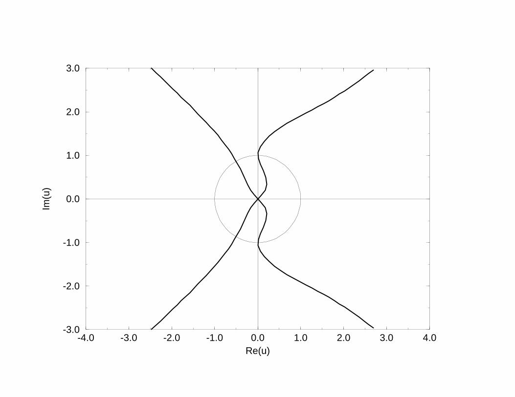
As shown in Fig. 1(a), the phase diagram consists of four phases, the complex-temperature

extension of the PM phase, together with three O phases. The curves separating these

phases are the solutions of |λ1,1| = |λ1,2|. The third eigenvalue, λ1,3, is always subdominant.

In the two phases containing the real us axis, λ1,2 has maximal magnitude, while in the

two containing the imaginary us axis, λ1,1 is dominant. The CT zeros of Z calculated for

finite lattices lie on or close to these curves, starting a finite distance from the origin and

being distributed in a manner symmetric under the inversion us → 1/us. As the lattice size

increases, the zeros spread out, the one with smallest (largest) magnitude moving closer to

(farther from) the origin. For s = 3/2, the eigenvalues are given by

2u9/4λ3/2,j = (1 + u2)(1 + ηu5/2)

ζ[

(1 − 2u2 + 4u3 + u4 + u5 + 4u6 − 2u7 + u9) − 2ηu5/2(1 − 6u2 + u4)]1/2

(4)

where here u ≡ u3/2 and (η, ζ) = (+, +), (−, +), (+,−), (−,−) for j = 1, 2, 3, 4. The phase

diagram is shown in Fig. 1(b) and consists of nine regions separated by the curves where

|λ3/2,1| = |λ3/2,2|. In the region containing the positive real us axis, λ3/2,1 is dominant, and

as one makes a circle around the origin, each of the nine times that one crosses a boundary,

there is an alternation between λ3/2,1 and λ3/2,2 as the dominant eigenvalue.

We find the following results for general s: (i) the complex-temperature phase diagram

consists of

Nc,1D = 4s2 (5)

(infinite) regions separated by an equal number of boundary curves where the free energy is

non-analytic; (ii) these curves extend from the origin to complex infinity, and in both limits

are oriented along the angles

θn =(1 + 2n)π

4s2(6)

3

for n = 0, ...4s2 − 1; (iii) of these curves, there are

Nc,NE,1D = Nc,NW,1D = [s2] (7)

in the first and second (NE and NW) quadrants, where [x] denotes the integral part of x;

and (iv) there is a boundary curve (which in this case is a straight line) along the negative

real us axis if and only if s is half-integral. (Nc,SE,1D = Nc,NE,1D and Nc,SW,1D = Nc,NW,1D

by the u → u∗ symmetry.) To derive these results, we carry out a Taylor series expansion of

the λs,j in the vicinity of us = 0. The dominant eigenvalues have the form

us2

s λs,j = 1 + ... + as,ju2s2

s + ... (8)

where the first ... dots denote terms which are independent of j and the second ... dots

represent higher order terms which are dependent upon j. Setting us = reiθ and solving the

equation |λs,j| = |λs,ℓ| yields cos(2s2θ) = 0, whence

2s2θ =π

2+ nπ , n = 0, ...4s2 − 1 (9)

Each of these solutions yields a curve across which f is non-analytic, corresponding to a

switching of dominant eigenvalue. These curves cannot terminate since if they did, one

could analytically continue from a region where the expression for f depends on a given

dominant eigenvalue, to a region where it depends on a different eigenvalue. Owing to the

us → 1/us symmetry of the model, a given curve labelled by n approaches complex infinity

in the same direction θn as it approaches the origin. This yields (i) and (ii). From (6), it

follows that

0 < θn < π/2 for 0 ≤ n < [s2 − 1/2] (10)

which comprises [s2] values, and similarly,

π/2 < θn < π for [s2 − 1/2] < n < [2s2 − 1/2] (11)

which again comprises [s2] values. Finally, if and only if s is half-integral, then the equation

θn = π has a solution (for integral n), viz., n = (2s + 1)(2s − 1)/2. From the us → u∗s

symmetry of the phase diagram, the curve corresponding to this solution must lie on the

negative real axis for all r, not just r → 0 and r → ∞. This yields (iii)-(iv). 2.

We note that from (6), the angular size of each region near the origin (or infinity) is

∆θ =π

2s2(12)

Also, from the us → u∗s symmetry of the phase diagram, it follows in particular, that for

each curve starting out from the origin at θn, there is a complex conjugate curve at −θn. As

4

is true of any theory at its lower critical dimensionality, the model is singular at K = ∞, i.e,

us = 0. If and only if s is integral, the n’th curve has another, m’th curve which is related

to it by θm = θn + π (whence m = n + 2s2), so that as one travels through the origin on the

n’th curve, one emerges on the other side on the m’th curve.

As one can see from Fig. 1, as the boundary curves approach the unit circle |us| = 1, some

of them twist in s-dependent ways. Interestingly, several of the points where they cross the

unit circle coincide with points which we inferred to be likely multiple (=intersection) points

of the boundary curves of the complex-temperature phase diagrams for the corresponding

spin s 2D Ising model. For example, for the 1D s = 1 model, the n = 0 and n = 1 curves cross

the unit circle at u1 = i and u1 = e2iπ/3, respectively, and hence the complex-conjugate curves

(n = 3 and n = 2) cross this circle at u1 = −i and u1 = e−2iπ/3. The points u1 = e±2iπ/3 are

precisely the values which we inferred for the intersection points of boundary curves in the

second (“northwest”=NW) and third (SW) quadrants of the 2D s = 1 phase diagram from

our calculation of partition function zeros [1]. For the 1D s = 3/2 case, the n = 0, 1, 2 and 3

curves cross the unit circle at the respective points u3/2 = eiπ/3, e2iπ/5, i, and e4iπ/5, and so

forth for the complex conjugate curves. Among these, the points ±i and e±4iπ/5 are points

inferred as likely intersection points of phase boundaries in the NW and SW quadrants of

the u3/2 plane for the 2D s = 3/2 model [1]. Similar correspondences hold for s = 2. These

are intriguing results.

The spin 1/2 Ising model is equivalent to the two-state Potts model. While determining

the CT phase diagram of the 1D spin s Ising model, it is thus also of interest to compare

this with that of the 1D q-state Potts model, defined by ZP =∑

σne−βHP with HP =

−JP∑

<nn′> δσnσn′

where σn ∈ {1, ..., q}. We define KP = βJP and uP = e−KP . 3 The

eigenvalues of the transfer matrix are λ = u−1

P − 1 (q − 1 times) and λ′ = u−1

P + (q − 1).

Setting uP = reiθ, the equation for |λ| = |λ′| is

q(

(q − 2)r + 2 cos θ)

= 0 (13)

For q = 2, the solution is the imaginary axis, uP = ±ir, equivalent to the negative real

axis in the u1/2 variable. For q 6= 2 (and q 6= 0 ), the solution is cos θ = −(q − 2)r/2 for

0 ≤ r ≤ 2/(q − 2), i.e.,

uP =−1 + eiω

q − 2(14)

for 0 ≤ ω < 2π, viz., a circle centered at uP = −1/(q − 2) with radius 1/(q − 2). Thus, for

all q > 2, the complex-temperature phase diagram is qualitatively the same, consisting of a

3Recall that the equivalence of HP for q = 2 to (1) for s = 1/2 entails KP = 2K.

5

PM phase containing the positive real u axis, and an O phase inside the circle (14).4 This

is quite different from the 1D spin s Ising phase diagram, for which the number of phases

does depend on s. This difference can be traced to the fact that the structure of the transfer

matrix is qualitatively the same for different q in the Potts model (all diagonal entries equal

to u−1 and all off-diagonal entries equal to 1), whereas it depends on s in the Ising model.

In addition to the correspondences already above, we have found a further very interesting

connection between the features of the 1D spin s Ising model and certain properties which

we have observed from our calculations of partition function zeros for the 2D (square-lattice)

Ising model with s = 1, 3/2, and 2 [1]. One of the interesting features which we found in

the 2D case was a certain number of finite arcs which protrude into the FM phase. (By the

us → 1/us symmetry, there are also corresponding arcs protruding into the AFM phase).

By combining our results with low-temperature series analyses in Refs. [2, 3], we observed

that the divergences of the spontaneous magnetization M (which also imply divergences in

the susceptibility [10]) occur at the endpoints of these arcs. The arc endpoints are thus of

considerable interest for the study of CT singularities.

For the cases s = 1, 3/2, and 2, the numbers of arcs protruding into and terminating in

the first and second (NE and NW) quadrants of the (complex-temperature extension of the)

FM phase are given in terms of the numbers of boundary curves of the corresponding 1D

spin s model as

Ne,NE,2D = Nc,NE,1D − 1 = [s2] − 1 (15)

and

Ne,NW,2D = Nc,NW,1D = [s2] (16)

so that the total number of arcs protruding into the FM (equivalently, AFM) phase is 4[s2]−2.

Our derivations in the present paper thus provide the explanation underlying our conjecture

[1] that the total number of arcs protruding into the FM (equivalently AFM) phase for the

Ising model on the square lattice with arbitrary spin s is

Ne,FM = Ne,AFM = max{0, 4[s2] − 2} (17)

where we have incorporated also the exact result that Ne,FM = Ne,AFM = 0 for s = 1/2.

One can qualitatively describe how the complex-temperature phase diagram changes as

one goes from d = 1 to d = 2 as follows. For d > 1, the model is analytic in the vicinity

of us = 0 (equivalently, it has a low-temperature series expansion with finite radius of

convergence), so one knows that all of the 4s2 curves which emanate from us = 0 must move

4One may also formally consider other values of q, as in the 2D Potts model. In particular, for q = 0, alleigenvalues are identically equal, and the phase diagram is trivial.

6

away from the origin. Evidently, the inner branches of the n = 0 curve and its complex

conjugate (n = 4s2 − 1) curve move to the right and join at the point (us)c = e−Kc/s2

which constitutes the critical point between the FM and PM phases; given the us → 1/us

symmetry, this means that the outer branches no longer run separately to complex infinity

but join each other at the critical point 1/(us)c separating the PM and AFM phases of

the 2D model. This leaves [s2] − 1 curves in the first (NE) quadrant, which form finite

arcs; the inner and outer branches of these arcs protrude into and terminate in the FM and

AFM phases respectively (these branches and phases are interchanged by the us → 1/us

mapping). The situation in the complex conjugate fourth (SE) quadrant is the same, by the

us → u∗s symmetry of the phase diagram. In the second (NW) quadrant, the [s2] curves in

1D correspond to the [s2] arcs in 2D, which again have inner and outer branches terminating

in the FM and AFM phases. The symmetry under complex conjugation implies the same

for the third (SW) quadrant.

In summary, we have found an intriguing connection between the complex-temperature

phase diagrams, as calculated exactly for 1D and inferred from partition function zeros for

2D, of the Ising model with higher spin. Our derivations here explain the basis for the

conjecture that we made in Ref. [1] on the total number of arc endpoints in the FM phase

and hence complex-temperature divergences in the magnetization for the square–lattice Ising

model with arbitrary spin.

This research was supported in part by the NSF grant PHY-93-09888.

References

[1] V. Matveev, and R. Shrock, “Zeros of the Partition Function for Higher–Spin 2D Ising

Models” ITP-SB-95-9 (hep-lat/9505005).

[2] I. G. Enting, A. J. Guttmann, and I. Jensen, J. Phys. A27 (1994) 6987.

[3] I. Jensen, A. J. Guttmann, and I. G. Enting, “Low-Temperature Series Expansions for

the Square Lattice Ising Model with Spin S > 1”, Melbourne draft, and A. J. Guttmann,

private communications.

[4] A. A. Migdal, Zh. Eksp. Teor. Fiz. 69 (1975) 1457 (JETP 42 (1975) 743); A. M.

Polyakov, Phys. Lett. B59 (1975) 79; E. Brezin and J. Zinn-Justin, Phys. Rev. Lett. 36

(1976) 691; Phys. Rev. B14 (1976) 3110; W. A. Bardeen, B. W. Lee, and R. E. Shrock,

Phys. Rev. D14 (1976) 985.

7

[5] M. E. Fisher, Lectures in Theoretical Physics (Univ. of Colorado Press, Boulder, 1965),

vol. 12C, p. 1.

[6] P. F. Fox and A. J. Guttmann, J. Phys. C6 (1973) 913.

[7] J. Ashkin and W. E. Lamb, Phys. Rev. 64 (1943) 159.

[8] V. Matveev and R. Shrock, J. Phys. A 28 (1995) 1557.

[9] V. Matveev and R. Shrock, J. Phys. A 28, in press (hep-lat/9412105).

[10] V. Matveev and R. Shrock, ITP-SB-94-53 (hep-lat/9411023).

8

Figure Captions

Fig. 1. Complex-temperature phase diagrams in the us plane for the 1D Ising model

with (a) s = 1 (with u ≡ u1) and (b) s = 3/2 (with u ≡ u3/2). The phase boundaries are

shown as the dark curves (including the line along the negative us axis for s = 3/2). The

unit circle is drawn in lightly for reference.

9

-4.0 -3.0 -2.0 -1.0 0.0 1.0 2.0 3.0 4.0Re(u)

-3.0

-2.0

-1.0

0.0

1.0

2.0

3.0

Im(u

)

-2.0 -1.6 -1.2 -0.8 -0.4 0.0 0.4 0.8 1.2 1.6 2.0Re(u)

-1.5

-1.0

-0.5

0.0

0.5

1.0

1.5

Im(u

)