UNCORRECTEDPROOF

1 ORIGINAL PAPER

2 A comprehensive study of surface and upper-air

3 characteristics over two stations on the west coast

4 of India during the occurrence of a cyclonic storm

5 Jagabandhu Panda • R. K. Giri

6 Received: 11 April 2011 /Accepted: 5 July 20127 � Springer Science+Business Media B.V. 2012

8 Abstract While qualitative information from meteorological satellites has long been

9 recognized as critical for monitoring weather events such as tropical cyclone activity,

10 quantitative data are required to improve the numerical prediction of these events. In this

11 paper, the sea surface winds from QuikSCAT, cloud motion vectors and water vapor winds

12 from KALPANA-1 are assimilated using three-dimensional variational assimilation tech-

13 nique within Weather Research Forecasting (WRF) modeling system. Further, the sensi-

14 tivity experiments are also carried out using the available cumulus convective

15 parameterizations in WRF modeling system. The model performance is evaluated using

16 available observations, and both qualitative and quantitative analyses are carried out while

17 analyzing the surface and upper-air characteristics over Mumbai (previously Bombay) and

18 Goa during the occurrence of the tropical cyclone PHYAN at the west coast of Indian

19 subcontinent. The model-predicted surface and upper-air characteristics show improve-

20 ments in most of the situations with the use of the satellite-derived winds from QuikSCAT

21 and KALPANA-1. Some of the model results are also found to be better in sensitivity

22 experiments using cumulus convection schemes as compared to the CONTROL

23 simulation.

24 Keywords WRF � 3DVAR � QuikSCAT � KALPANA-1 � PHYAN �25 Surface and upper-air characteristics

A1 J. Panda � R. K. GiriA2 Satellite Meteorology Division, India Meteorological Department, Lodhi Road, New Delhi 110003,

India

A3 Present Address:

A4 J. Panda (&)

A5 School of Physical and Mathematical Sciences, SPMS 04-19, Nanyang Technological University,

A6 21 Nanyang Link, Singapore 637371, Singapore

A7 e-mail: jagabandhu@gmail.com; jpanda@ntu.edu.sg

123

Journal : Small 11069 Dispatch : 10-7-2012 Pages : 24

Article No. : 282 h LE h TYPESET

MS Code : NHAZ1589 h CP h DISK4 4

Nat Hazards

DOI 10.1007/s11069-012-0282-6

Au

tho

r P

ro

of

UNCORRECTEDPROOF

26 1 Introduction

27 The tropical cyclonic storms normally occur over warm waters of the Bay of Bengal and

28 the Arabian Sea, when the central pressure falls by 5–6 hPa from the surroundings of a

29 low-pressure system under favorable situation, and the wind speed is as high as 17.5 m/s or

30 even greater. The cyclonic storm becomes dangerous with the increase in the drop of

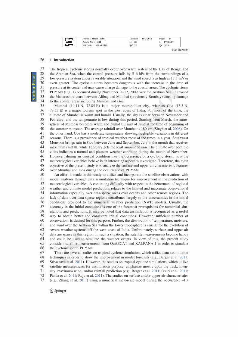
31 pressure at its center and may cause a large damage to the coastal areas. The cyclonic storm

32 PHYAN (Fig. 1) occurred during November, 8–12, 2009 over the Arabian Sea. It crossed

33 the Maharashtra coast between Alibag and Mumbai (previously Bombay) causing damage

34 to the coastal areas including Mumbai and Goa.

35 Mumbai (19.11 N, 72.85 E) is a major metropolitan city, whereas Goa (15.3 N,

36 73.55 E) is a major tourism spot in the west coast of India. For most of the time, the

37 climate of Mumbai is warm and humid. Usually, the sky is clear between November and

38 February, and the temperature is low during this period. Starting from March, the atmo-

39 sphere of Mumbai becomes warm and humid till mid of June at the time of beginning of

40 the summer monsoon. The average rainfall over Mumbai is 180 cm (Singh et al. 2008). On

41 the other hand, Goa has a moderate temperature showing negligible variations in different

42 seasons. There is a prevalence of tropical weather most of the times in a year. Southwest

43 Monsoon brings rain in Goa between June and September. July is the month that receives

44 maximum rainfall, while February gets the least amount of rain. The climate over both the

45 cities indicates a normal and pleasant weather condition during the month of November.

46 However, during an unusual condition like the occurrence of a cyclonic storm, how the

47 meteorological variables behave is an interesting aspect to investigate. Therefore, the main

48 objective of the present study is to analyze the surface and upper-air characteristic features

49 over Mumbai and Goa during the occurrence of PHYAN.

50 An effort is made in this study to utilize and incorporate the satellite observations with

51 model analyses through data assimilation technique for improvement in the prediction of

52 meteorological variables. A continuing difficulty with respect to the betterment of regional

53 weather and climate model predictions relates to the limited and inaccurate observational

54 information especially over data-sparse areas over oceans and other remote regions. The

55 lack of data over data-sparse regions contributes largely to the uncertainties in the initial

56 conditions provided to the numerical weather prediction (NWP) models. Usually, the

57 accuracy in the initial conditions is one of the foremost prerequisites for numerical sim-

58 ulations and predictions. It may be noted that data assimilation is recognized as a useful

59 way to obtain better and consistent initial conditions. However, sufficient number of

60 observations is desired for this purpose. Further, the distribution of temperature, moisture,

61 and wind over the Arabian Sea within the lower troposphere is crucial for the evolution of

62 severe weather systems off the west coast of India. Unfortunately, surface and upper-air

63 data are sparse in this region. In such a situation, the satellite measurements become handy

64 and could be used to simulate the weather events. In view of this, the present study

65 considers satellite measurements from QuikSCAT and KALPANA-1 in order to simulate

66 the cyclonic storm PHYAN.

67 There are several studies on tropical cyclone simulation, which utilize data assimilation

68 techniques in order to show the improvement in model forecasts (e.g., Berger et al. 2011;

69 Srivastava et al. 2011). However, the studies on tropical cyclone simulations, which utilize

70 satellite measurements for assimilation purpose, emphasize mostly upon the track, inten-

71 sity, maximum wind, and/or rainfall prediction (e.g., Berger et al. 2011; Osuri et al. 2011;

72 Panda et al. 2011; Raju et al. 2011). The studies on surface and/or upper-air characteristics

73 (e.g., Zhang et al. 2011) using a numerical mesoscale model during the occurrence of a

Nat Hazards

123

Journal : Small 11069 Dispatch : 10-7-2012 Pages : 24

Article No. : 282 h LE h TYPESET

MS Code : NHAZ1589 h CP h DISK4 4

Au

tho

r P

ro

of

UNCORRECTEDPROOF

Fig. 1 Satellite images during the occurrence of the cyclone PHYAN: aQSCATwind vectors duringmorning

pass on November 09, 2009 and b KALPANA-1 infrared (IR) image at 02 UTC, November 11, 2009

Nat Hazards

123

Journal : Small 11069 Dispatch : 10-7-2012 Pages : 24

Article No. : 282 h LE h TYPESET

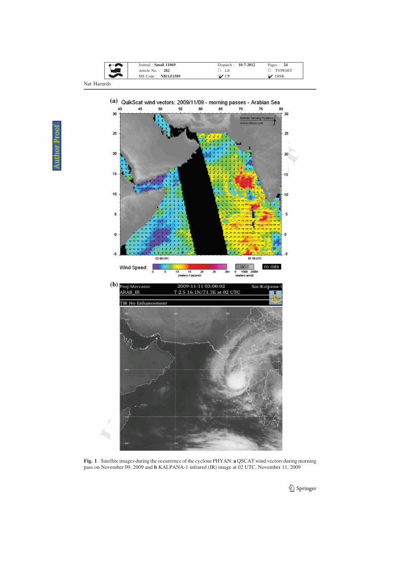
MS Code : NHAZ1589 h CP h DISK4 4

Au

tho

r P

ro

of

UNCORRECTEDPROOF

74 tropical cyclone are limited in literature. In view of these, the present work incorporates the

75 QuickSCAT surface winds and KALPANA-1 atmospheric motion vectors (combination of

76 cloud motion vectors (CMV) and water vapor winds) with the model initial and boundary

77 conditions using three-dimensional variational (3DVAR) technique to simulate the weather

78 event using WRF (Weather Research and Forecasting) modeling system and study the

79 surface and upper-air characteristic features over Mumbai and Goa.

80 Further, the development and propagation of a tropical cyclone is largely dependent

81 upon the prevailing convective condition of the atmosphere. Therefore, the cumulus

82 convection physics plays a vital role in the simulation of such an event. In view of this, the

83 present study also takes into account the sensitivity to cumulus schemes available in WRF

84 modeling system. The details of the numerical model, experimental design, and data used

85 in this study are described in the following section.

86 2 Numerical model, experimental design, and data used

87 2.1 Numerical model and experimental design

88 The present study uses WRF modeling system version 3.1.1 (Skamarock et al. 2008). It has

89 been developed by a multi-institutional effort and is quite robust for research and opera-

90 tional purpose since it contains advanced dynamics, physics, and numerical schemes like

91 that of MM5 model (Grell et al. 1994). Several studies have already used the model in past

92 for simulating local and mesoscale events (e.g., Anil Kumar et al. 2008; Lin et al. 2008;

93 Miao et al. 2009; Routray et al. 2010).

94 The WRF modeling system uses a set of governing equations based on conservation of

95 mass, momentum, energy, and scalars such as moisture (Ooyama 1990). These equations

96 are written in flux form on an Eulerian solver and use mass-based vertical ‘‘g’’ co-ordinate

97 that varies from 1 at the surface to 0 at the upper boundary of the model domain. The

98 prognostic variables in the equations are dry air mass, velocity components u (zonal wind

99 component), v (meridional wind component), and w (vertical wind component), potential

100 temperature (h), and geopotential (u). The non-conserved variables such as temperature

101 (T), pressure (p), and density (q) are diagnosed from the conserved prognostic variables.

102 These equations are solved using initial and periodic boundary conditions as provided to

103 the model.

104 In the present study, the model is primarily initialized with six hourly NCEP (National

105 Center for Environmental Prediction)/NCAR (National Center for Atmospheric Research)

106 global final analysis data (or FNL global analysis data) of 1� 9 1� resolution

107 (http://dss.ucar.edu/datasets/ds083.2/data/) at 0000 UTC November 09, 2009. The initiali-

108 zation process is carried out through the preprocessing package named WPS that defines the

109 physical grid, interpolates the static fields (terrestrial data) from USGS (United States

110 Geological Survey) global data and themeteorological data from global analysis to themodel

111 coordinates in both horizontal and vertical directions within the specified domain.

112 The domain considered for this study includes a large part of the Arabian Sea as well as

113 the Bay of Bengal (Fig. 2a). The resolution of the domain is taken as 27 km with 121 grid

114 points along both the horizontal directions, and the vertical resolution of the model con-

115 tains 38 ‘‘g’’ levels (Table 1). At the top of the model grid, pressure of 50 hpa is considered

116 to be constant for all simulations. The central latitude and longitude for all experiments are

117 taken to be 16.5 N and 74.0 E, respectively (Table 1).

Nat Hazards

123

Journal : Small 11069 Dispatch : 10-7-2012 Pages : 24

Article No. : 282 h LE h TYPESET

MS Code : NHAZ1589 h CP h DISK4 4

Au

tho

r P

ro

of

UNCORRECTEDPROOF

118 The simulation of the cyclone PHYAN (Fig. 1) uses a set of physics options containing

119 short-wave radiation parameterization from Dudhia (1989), Rapid Radiative Transfer

120 Model (RRTM) for long-wave radiation (Mlawer et al. 1997), WRF single-moment three-

121 class scheme (Dudhia 1989; Hong et al. 2004; Hong and Lim 2006) for microphysics,

122 Grell-Devenyi (GD) ensemble scheme (Grell and Devenyi 2002) for cumulus convection,

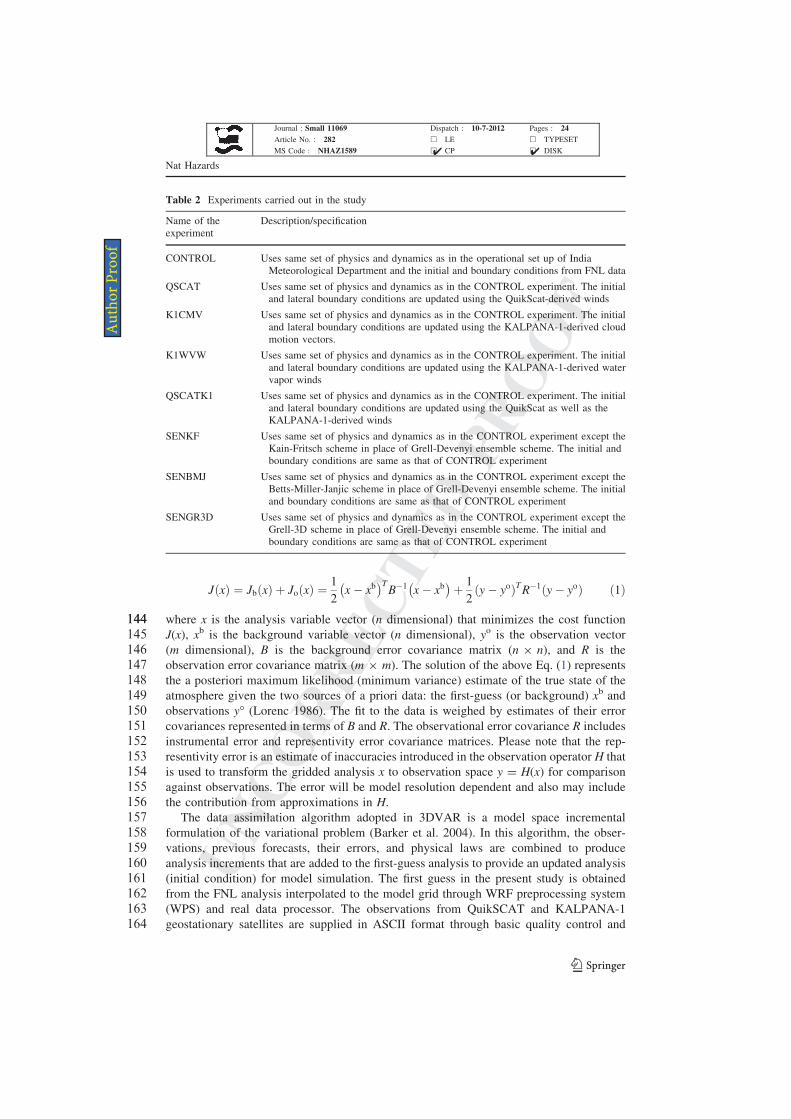
123 Unified Noah land surface model (Chen and Dudhia 2001) and Yonsei University (YSU)

124 boundary layer scheme (Hong et al. 2006). These parameterization schemes are chosen for

125 the CONTROL simulation in order to maintain the consistency with the operational setting

126 used for numerical weather forecasting purpose at India Meteorological Department

127 (IMD). The simulations carried out in the present study take into account cloud cover

128 effect. However, snow cover effect is not included. All the simulations are done in non-

129 hydrostatic mode and use second-order diffusion in coordinate surface.

130 The sensitivity studies carried out in this study consider all the physics and dynamics as

131 that of CONTROL experiment except the cumulus convection schemes. The cumulus

132 schemes are as follows: (i) Kain-Fritsch (KF) scheme (Kain and Fritsch 1990, 1993; Kain

Fig. 2 Domain used and data considered for the assimilation of satellite-derived winds during the

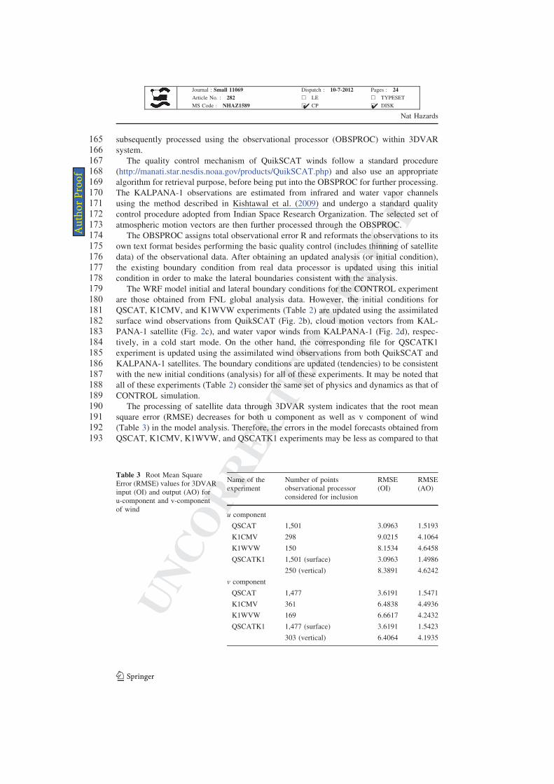
occurrence of the cyclone PHYAN: a Domain used in the present study, b QSCAT surface wind vectors

during morning pass on November 09, 2009, c KALPANA-1 cloud motion vectors at 00 UTC November 09,

2009, and d KALPANA-1 water vapor winds at 00 UTC November 09, 2009

Nat Hazards

123

Journal : Small 11069 Dispatch : 10-7-2012 Pages : 24

Article No. : 282 h LE h TYPESET

MS Code : NHAZ1589 h CP h DISK4 4

Au

tho

r P

ro

of

UNCORRECTEDPROOF

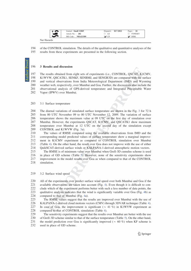
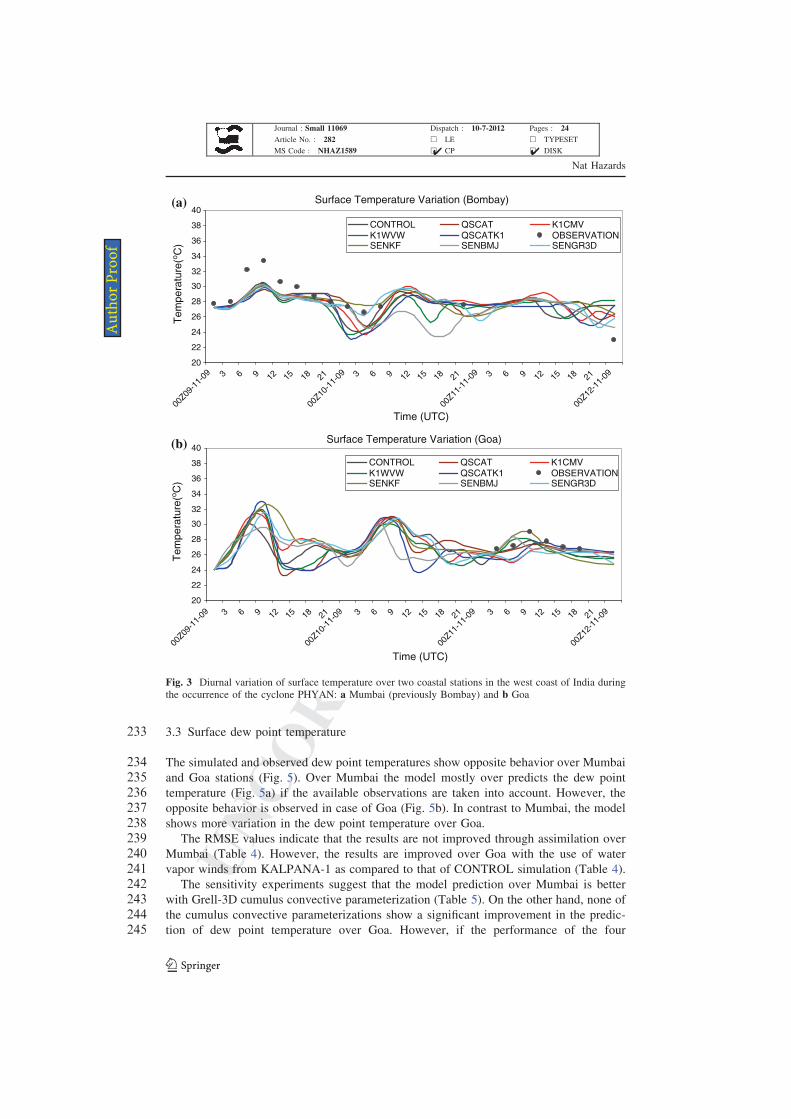
133 2004), (ii) Betts-Miller-Janjic (BMJ) scheme (Betts and Miller 1986; Janjic 2000), (iii)

134 Grell-Devenyi (GD) ensemble scheme (Grell and Devenyi 2002), and (iv) Grell-3D

135 cumulus parameterization (Grell and Devenyi 2002). The KF scheme, BMJ scheme, and

136 Grell-3D scheme are used in SENKF, SENBMJ, and SENGR3D experiments, respectively

137 (Table 2). In these sensitivity experiments, the initial and boundary conditions are kept

138 unchanged as that of CONTROL simulation (i.e., the FNL data are used in these simu-

139 lations as well).

140 2.2 Assimilation methodology and experiments

141 The 3DVAR technique (Barker et al. 2004) within WRF modeling system was imple-

142 mented by minimizing the cost function (Ide et al. 1997) defined as:

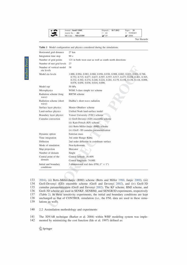
Table 1 Model configuration and physics considered during the simulations

Horizontal grid distance 27 km

Integration time step 90 s

Number of grid points 121 in both west–east as well as south–north directions

Number of met grid levels 27

Number of vertical model

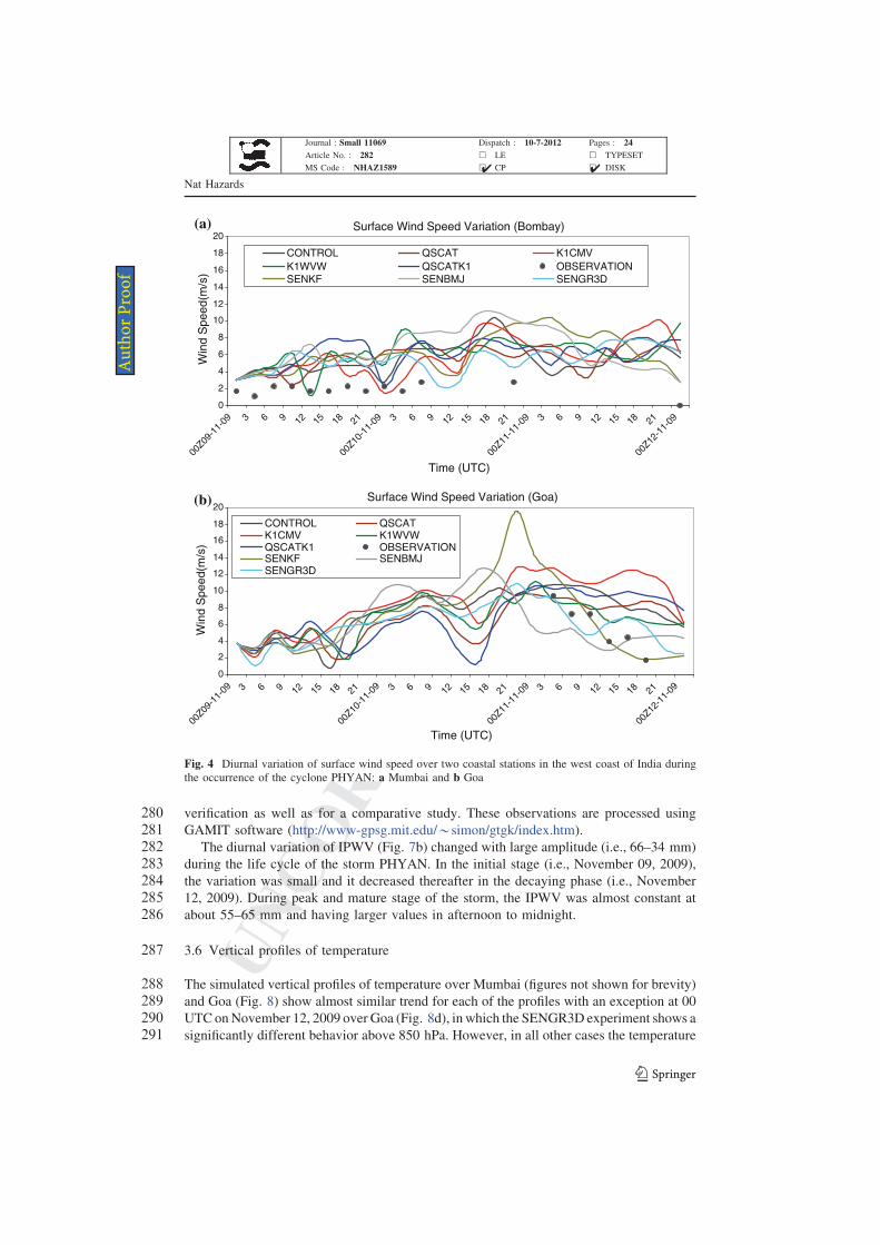
eta levels

38

Model eta levels 1.000, 0.994, 0.983, 0.968, 0.950, 0.930, 0.908, 0.882, 0.853, 0.821, 0.788,

0.752, 0.715, 0.677, 0.637, 0.597, 0.557, 0.517, 0.477, 0.438, 0.401, 0.365,

0.332, 0.302, 0.274, 0.248, 0.224, 0.201, 0.179, 0.158, 0.138, 0.118, 0.098,

0.078, 0.058, 0.038, 0.018, 0.000,

Model top 50 hPa

Microphysics WSM 3-class simple ice scheme

Radiation scheme (long

wave)

RRTM scheme

Radiation scheme (short

wave)

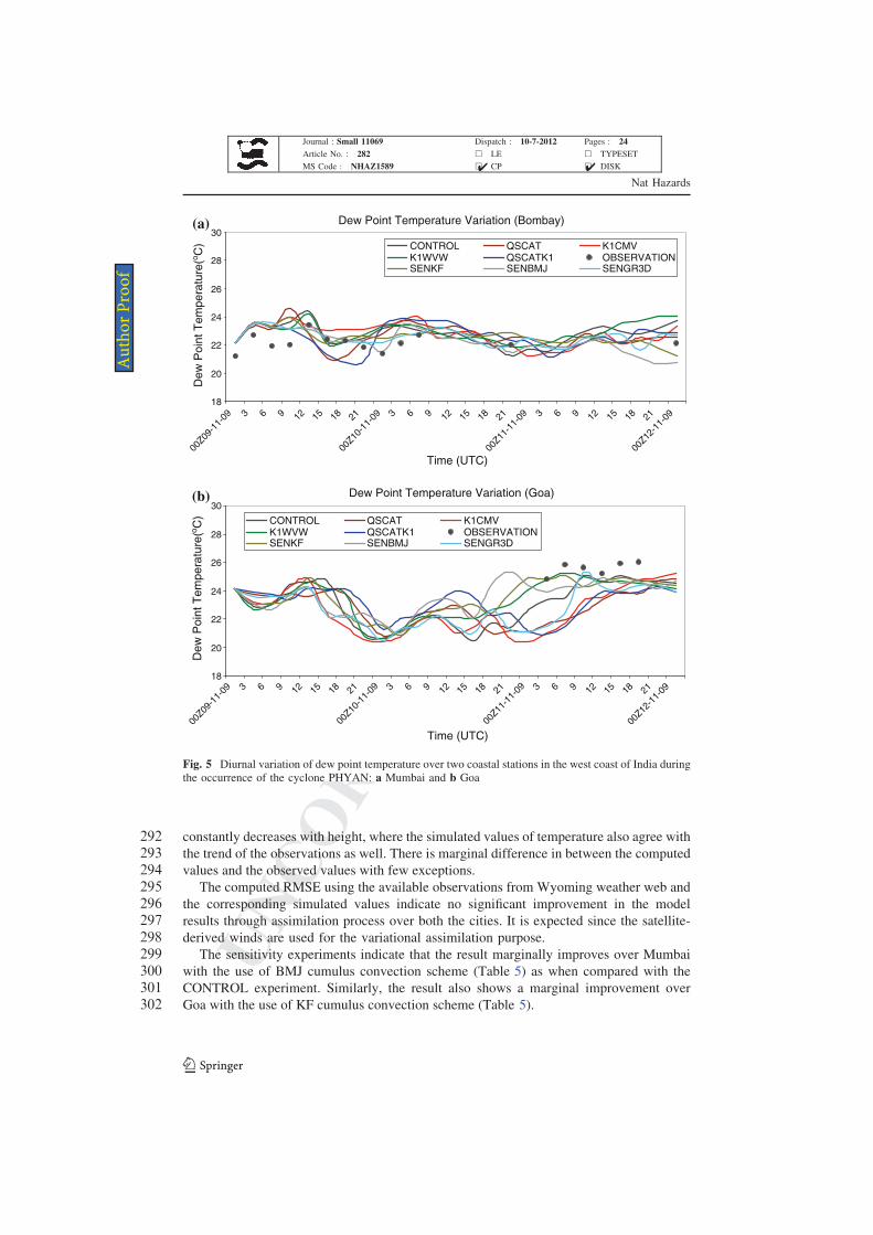
Dudhia’s short-wave radiation

Surface layer physics Monin–Obukhov scheme

Land-surface physics Unified Noah land-surface model

Boundary layer physics Yonsei University (YSU) scheme

Cumulus convection (i) Grell-Devenyi (GD) ensemble scheme

(ii) Kain-Fritsch (KF) scheme

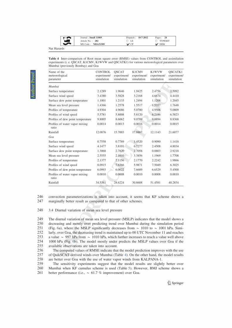
(iii) Betts-Miller-Janjic (BMJ) scheme

(iv) Grell -3D cumulus parameterization

Dynamic option Eulerian mass

Time integration 3rd order Runge–Kutta

Diffusion 2nd order diffusion in coordinate surface

Mode of simulation Non-hydrostatic

Map projection Mercator

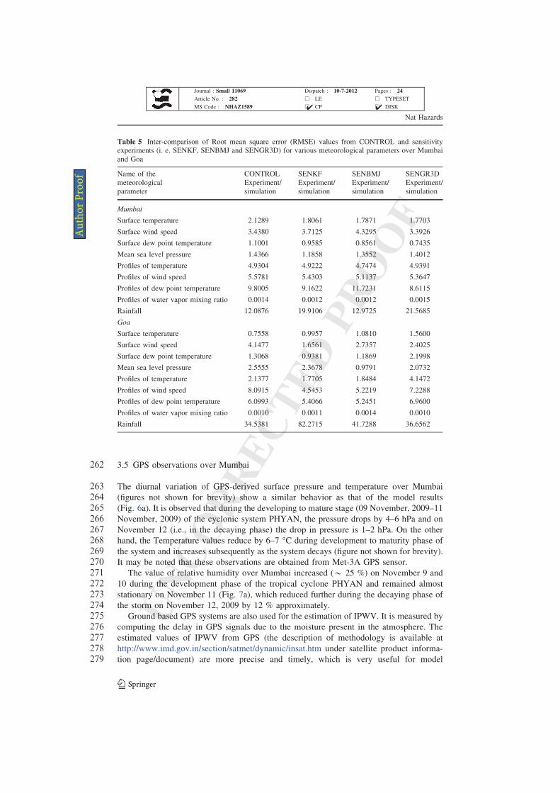
Number of domain Single

Central point of the

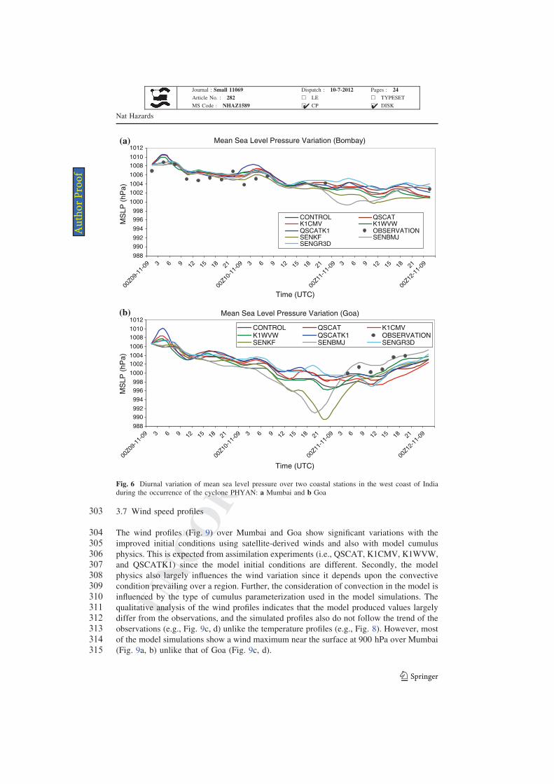
domain

Central latitude: 16.40N

Central longitude: 74.00E

Initial and boundary

conditions

3-dimensional real data (FNL:1� 9 1�)

Nat Hazards

123

Journal : Small 11069 Dispatch : 10-7-2012 Pages : 24

Article No. : 282 h LE h TYPESET

MS Code : NHAZ1589 h CP h DISK4 4

Au

tho

r P

ro

of

UNCORRECTEDPROOF

JðxÞ ¼ JbðxÞ þ JoðxÞ ¼1

2x� xb

� �TB�1 x� xb

� �

þ1

2y� yoð ÞTR�1 y� yoð Þ ð1Þ

144144 where x is the analysis variable vector (n dimensional) that minimizes the cost function

145 J(x), xb is the background variable vector (n dimensional), yo is the observation vector

146 (m dimensional), B is the background error covariance matrix (n 9 n), and R is the

147 observation error covariance matrix (m 9 m). The solution of the above Eq. (1) represents

148 the a posteriori maximum likelihood (minimum variance) estimate of the true state of the

149 atmosphere given the two sources of a priori data: the first-guess (or background) xb and

150 observations y� (Lorenc 1986). The fit to the data is weighed by estimates of their error

151 covariances represented in terms of B and R. The observational error covariance R includes

152 instrumental error and representivity error covariance matrices. Please note that the rep-

153 resentivity error is an estimate of inaccuracies introduced in the observation operator H that

154 is used to transform the gridded analysis x to observation space y = H(x) for comparison

155 against observations. The error will be model resolution dependent and also may include

156 the contribution from approximations in H.

157 The data assimilation algorithm adopted in 3DVAR is a model space incremental

158 formulation of the variational problem (Barker et al. 2004). In this algorithm, the obser-

159 vations, previous forecasts, their errors, and physical laws are combined to produce

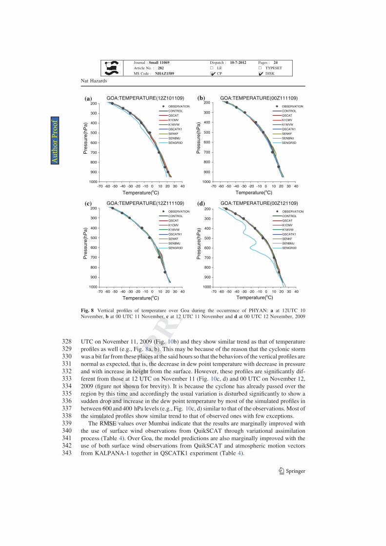
160 analysis increments that are added to the first-guess analysis to provide an updated analysis

161 (initial condition) for model simulation. The first guess in the present study is obtained

162 from the FNL analysis interpolated to the model grid through WRF preprocessing system

163 (WPS) and real data processor. The observations from QuikSCAT and KALPANA-1

164 geostationary satellites are supplied in ASCII format through basic quality control and

Table 2 Experiments carried out in the study

Name of the

experiment

Description/specification

CONTROL Uses same set of physics and dynamics as in the operational set up of India

Meteorological Department and the initial and boundary conditions from FNL data

QSCAT Uses same set of physics and dynamics as in the CONTROL experiment. The initial

and lateral boundary conditions are updated using the QuikScat-derived winds

K1CMV Uses same set of physics and dynamics as in the CONTROL experiment. The initial

and lateral boundary conditions are updated using the KALPANA-1-derived cloud

motion vectors.

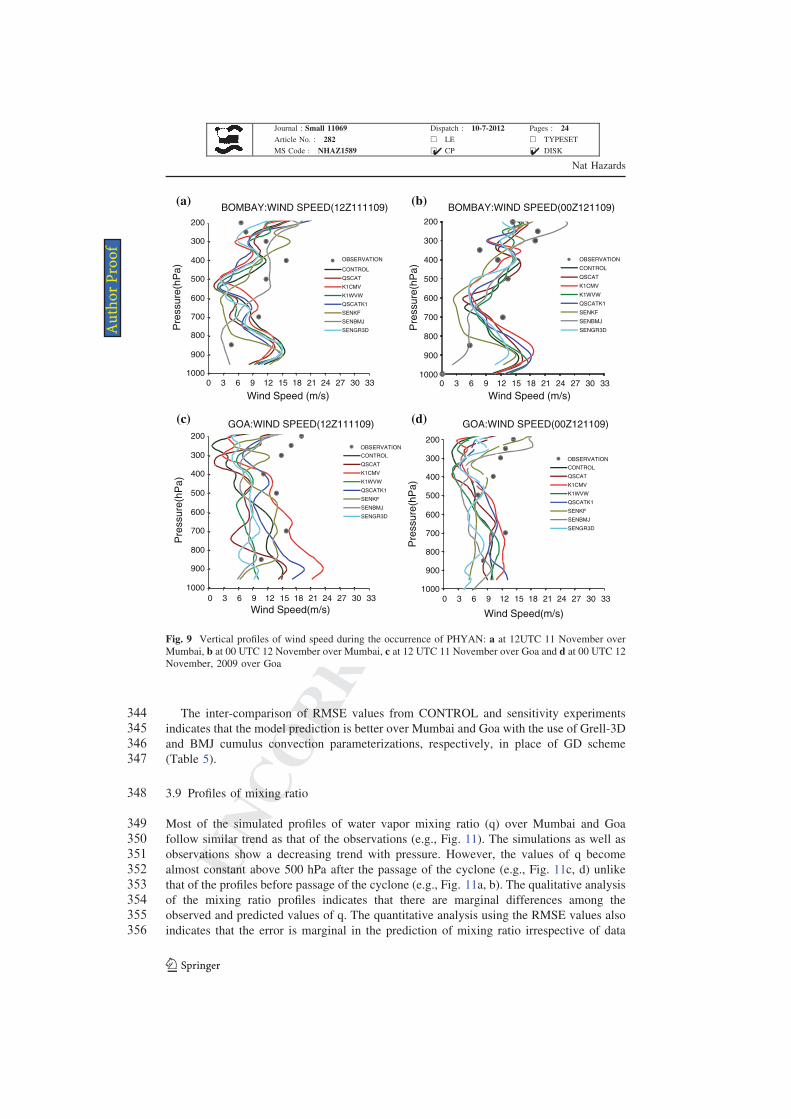
K1WVW Uses same set of physics and dynamics as in the CONTROL experiment. The initial

and lateral boundary conditions are updated using the KALPANA-1-derived water

vapor winds

QSCATK1 Uses same set of physics and dynamics as in the CONTROL experiment. The initial

and lateral boundary conditions are updated using the QuikScat as well as the

KALPANA-1-derived winds

SENKF Uses same set of physics and dynamics as in the CONTROL experiment except the

Kain-Fritsch scheme in place of Grell-Devenyi ensemble scheme. The initial and

boundary conditions are same as that of CONTROL experiment

SENBMJ Uses same set of physics and dynamics as in the CONTROL experiment except the

Betts-Miller-Janjic scheme in place of Grell-Devenyi ensemble scheme. The initial

and boundary conditions are same as that of CONTROL experiment

SENGR3D Uses same set of physics and dynamics as in the CONTROL experiment except the

Grell-3D scheme in place of Grell-Devenyi ensemble scheme. The initial and

boundary conditions are same as that of CONTROL experiment

Nat Hazards

123

Journal : Small 11069 Dispatch : 10-7-2012 Pages : 24

Article No. : 282 h LE h TYPESET

MS Code : NHAZ1589 h CP h DISK4 4

Au

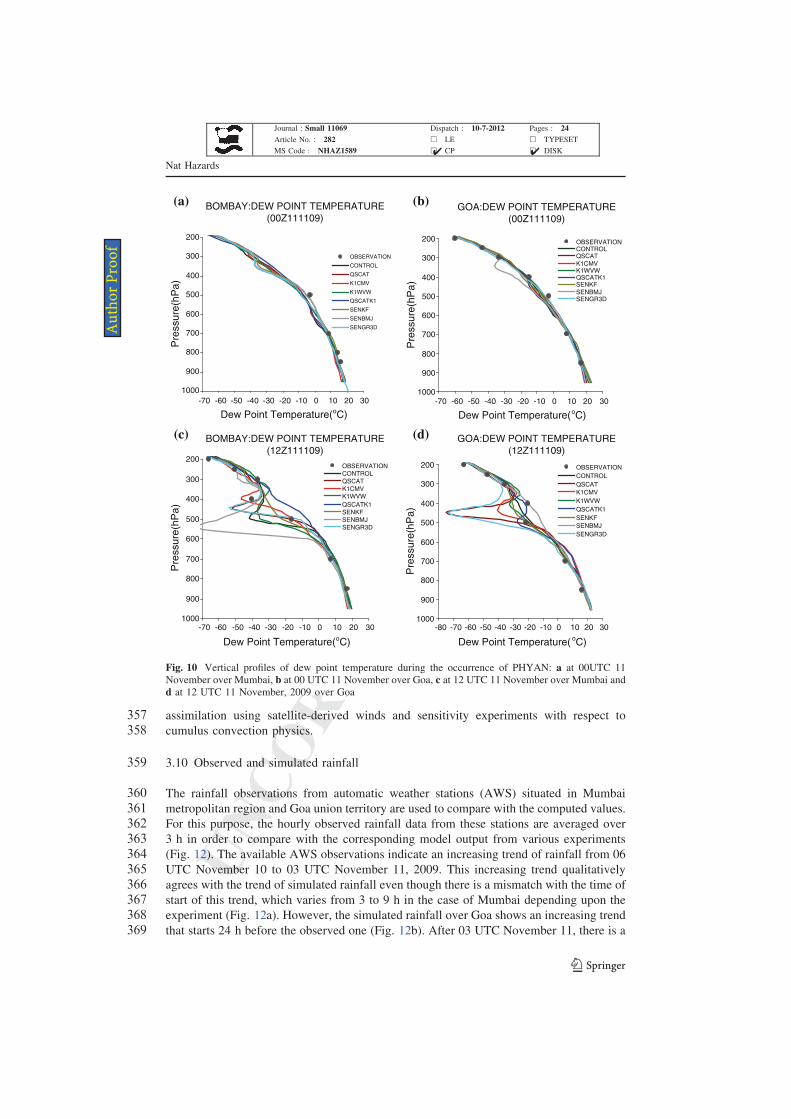
tho

r P

ro

of

UNCORRECTEDPROOF

165 subsequently processed using the observational processor (OBSPROC) within 3DVAR

166 system.

167 The quality control mechanism of QuikSCAT winds follow a standard procedure

168 (http://manati.star.nesdis.noaa.gov/products/QuikSCAT.php) and also use an appropriate

169 algorithm for retrieval purpose, before being put into the OBSPROC for further processing.

170 The KALPANA-1 observations are estimated from infrared and water vapor channels

171 using the method described in Kishtawal et al. (2009) and undergo a standard quality

172 control procedure adopted from Indian Space Research Organization. The selected set of

173 atmospheric motion vectors are then further processed through the OBSPROC.

174 The OBSPROC assigns total observational error R and reformats the observations to its

175 own text format besides performing the basic quality control (includes thinning of satellite

176 data) of the observational data. After obtaining an updated analysis (or initial condition),

177 the existing boundary condition from real data processor is updated using this initial

178 condition in order to make the lateral boundaries consistent with the analysis.

179 The WRF model initial and lateral boundary conditions for the CONTROL experiment

180 are those obtained from FNL global analysis data. However, the initial conditions for

181 QSCAT, K1CMV, and K1WVW experiments (Table 2) are updated using the assimilated

182 surface wind observations from QuikSCAT (Fig. 2b), cloud motion vectors from KAL-

183 PANA-1 satellite (Fig. 2c), and water vapor winds from KALPANA-1 (Fig. 2d), respec-

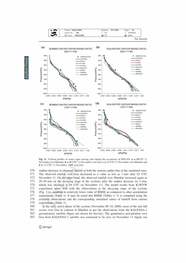
184 tively, in a cold start mode. On the other hand, the corresponding file for QSCATK1

185 experiment is updated using the assimilated wind observations from both QuikSCAT and

186 KALPANA-1 satellites. The boundary conditions are updated (tendencies) to be consistent

187 with the new initial conditions (analysis) for all of these experiments. It may be noted that

188 all of these experiments (Table 2) consider the same set of physics and dynamics as that of

189 CONTROL simulation.

190 The processing of satellite data through 3DVAR system indicates that the root mean

191 square error (RMSE) decreases for both u component as well as v component of wind

192 (Table 3) in the model analysis. Therefore, the errors in the model forecasts obtained from

193 QSCAT, K1CMV, K1WVW, and QSCATK1 experiments may be less as compared to that

Table 3 Root Mean Square

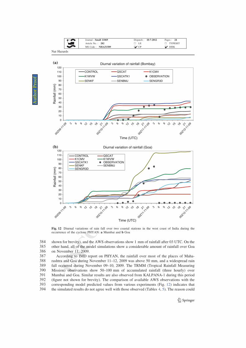
Error (RMSE) values for 3DVAR

input (OI) and output (AO) for

u-component and v-component

of wind

Name of the

experiment

Number of points

observational processor

considered for inclusion

RMSE

(OI)

RMSE

(AO)

u component

QSCAT 1,501 3.0963 1.5193

K1CMV 298 9.0215 4.1064

K1WVW 150 8.1534 4.6458

QSCATK1 1,501 (surface) 3.0963 1.4986

250 (vertical) 8.3891 4.6242

v component

QSCAT 1,477 3.6191 1.5471

K1CMV 361 6.4838 4.4936

K1WVW 169 6.6617 4.2432

QSCATK1 1,477 (surface) 3.6191 1.5423

303 (vertical) 6.4064 4.1935

Nat Hazards

123

Journal : Small 11069 Dispatch : 10-7-2012 Pages : 24

Article No. : 282 h LE h TYPESET

MS Code : NHAZ1589 h CP h DISK4 4

Au

tho

r P

ro

of

UNCORRECTEDPROOF

194 of the CONTROL simulation. The details of the qualitative and quantitative analyses of the

195 results from these experiments are presented in the following section.

196 3 Results and discussion

197 The results obtained from eight sets of experiments (i.e., CONTROL, QSCAT, K1CMV,

198 K1WVW, QSCATK1, SENKF, SENBMJ, and SENGR3D) are compared with the surface

199 and vertical observations from India Meteorological Department (IMD) and Wyoming

200 weather web, respectively, over Mumbai and Goa. Further, the discussions also include the

201 observational analysis of GPS-derived temperature and Integrated Precipitable Water

202 Vapor (IPWV) over Mumbai.

203 3.1 Surface temperature

204 The diurnal variations of simulated surface temperature are shown in the Fig. 3 for 72 h

205 from 00 UTC November 09 to 00 UTC November 12, 2009. The variation of surface

206 temperature shows the maximum value at 09 UTC on the first day of simulation over

207 Mumbai. However, the experiments QSCAT, K1CMV, and QSCATK1 show maximum

208 temperature over Mumbai at 12 UTC on the second day of the simulation except

209 CONTROL and K1WVW (Fig. 3a).

210 The values of RMSE computed using the available observations from IMD and the

211 corresponding model predicted values of surface temperature show a marginal improve-

212 ment in K1CMV experiment as compared to CONTROL simulation over Mumbai

213 (Table 4). On the other hand, the result over Goa does not improve with the use of either

214 QuikSCAT-derived surface winds or KALPANA-1-derived atmospheric motion vectors.

215 The RMSE is of minimum value over Mumbai when Grell-3D cumulus scheme is used

216 in place of GD scheme (Table 5). However, none of the sensitivity experiments show

217 improvement in the model results over Goa as when compared to that of the CONTROL

218 simulation.

219 3.2 Surface wind speed

220 All of the experiments over predict surface wind speed over both Mumbai and Goa if the

221 available observations are taken into account (Fig. 4). Even though it is difficult to con-

222 clude which of the experiment performs better with such a less number of data points, the

223 qualitative analysis indicates that the wind is significantly variable over Goa (Fig. 4b) as

224 compared to that of Mumbai (Fig. 4a).

225 The RMSE values suggest that the results are improved over Mumbai with the use of

226 KALPANA-1-derived cloud motions vectors (CMV) through 3DVAR technique (Table 4).

227 In case of Goa, the improvement is significant (* 41 %) in K1WVW experiment as

228 compared to that of CONTROL simulation (Table 4).

229 The sensitivity experiments suggest that the results over Mumbai are better with the use

230 of Grell-3D scheme similar to that of the surface temperature (Table 5). On the other hand,

231 the model prediction over Goa is significantly improved (* 60 %) when KF scheme is

232 used in place of GD scheme.

Nat Hazards

123

Journal : Small 11069 Dispatch : 10-7-2012 Pages : 24

Article No. : 282 h LE h TYPESET

MS Code : NHAZ1589 h CP h DISK4 4

Au

tho

r P

ro

of

UNCORRECTEDPROOF

233 3.3 Surface dew point temperature

234 The simulated and observed dew point temperatures show opposite behavior over Mumbai

235 and Goa stations (Fig. 5). Over Mumbai the model mostly over predicts the dew point

236 temperature (Fig. 5a) if the available observations are taken into account. However, the

237 opposite behavior is observed in case of Goa (Fig. 5b). In contrast to Mumbai, the model

238 shows more variation in the dew point temperature over Goa.

239 The RMSE values indicate that the results are not improved through assimilation over

240 Mumbai (Table 4). However, the results are improved over Goa with the use of water

241 vapor winds from KALPANA-1 as compared to that of CONTROL simulation (Table 4).

242 The sensitivity experiments suggest that the model prediction over Mumbai is better

243 with Grell-3D cumulus convective parameterization (Table 5). On the other hand, none of

244 the cumulus convective parameterizations show a significant improvement in the predic-

245 tion of dew point temperature over Goa. However, if the performance of the four

Surface Temperature Variation (Bombay)

20

22

24

26

28

30

32

34

36

38

40

00Z09

-11-

09 3 6 9 12 15 18 21

00Z10

-11-

09 3 6 9 12 15 18 21

00Z11

-11-

09 3 6 9 12 15 18 21

00Z12

-11-

09

Time (UTC)

Tem

pera

ture

(oC

)

CONTROL QSCAT K1CMVK1WVW QSCATK1 OBSERVATIONSENKF SENBMJ SENGR3D

(a)

Surface Temperature Variation (Goa)

20

22

24

26

28

30

32

34

36

38

40

00Z09

-11-

09 3 6 9 12 15 18 21

00Z10

-11-

09 3 6 9 12 15 18 21

00Z11

-11-

09 3 6 9 12 15 18 21

00Z12

-11-

09

Time (UTC)

Tem

pera

ture

(oC

)

CONTROL QSCAT K1CMVK1WVW QSCATK1 OBSERVATIONSENKF SENBMJ SENGR3D

(b)

Fig. 3 Diurnal variation of surface temperature over two coastal stations in the west coast of India during

the occurrence of the cyclone PHYAN: a Mumbai (previously Bombay) and b Goa

Nat Hazards

123

Journal : Small 11069 Dispatch : 10-7-2012 Pages : 24

Article No. : 282 h LE h TYPESET

MS Code : NHAZ1589 h CP h DISK4 4

Au

tho

r P

ro

of

UNCORRECTEDPROOF

246 convection parameterizations is taken into account, it seems that KF scheme shows a

247 marginally better result as compared to that of other schemes.

248 3.4 Diurnal variation of mean sea level pressure

249 The diurnal variation of mean sea level pressure (MSLP) indicates that the model shows a

250 decreasing and mostly over predicting trend over Mumbai during the simulation period

251 (Fig. 6a), where the MSLP significantly decreases from * 1010 to * 1001 hPa. Simi-

252 larly, over Goa, the decreasing trend is maintained up to 00 UTC November 11 and reaches

253 a value * 997 hPa from * 1010 hPa, which further increases to reach a value well above

254 1000 hPa (Fig. 6b). The model mostly under predicts the MSLP values over Goa if the

255 available observations are taken into account.

256 The computed values of RMSE indicate that the model prediction improves with the use

257 of QuikSCAT-derived winds over Mumbai (Table 4). On the other hand, the model results

258 are better over Goa with the use of water vapor winds from KALPANA-1.

259 The sensitivity experiments suggest that the model results are slightly better over

260 Mumbai when KF cumulus scheme is used (Table 5). However, BMJ scheme shows a

261 better performance (i.e., * 61.7 % improvement) over Goa.

Table 4 Inter-comparison of Root mean square error (RMSE) values from CONTROL and assimilation

experiments (i. e. QSCAT, K1CMV, K1WVW and QSCATK1) for various meteorological parameters over

Mumbai (previously Bombay) and Goa

Name of the

meteorological

parameter

CONTROL

experiment/

simulation

QSCAT

experiment/

simulation

K1CMV

experiment/

simulation

K1WVW

experiment/

simulation

QSCATK1

experiment/

simulation

Mumbai

Surface temperature 2.1289 1.9646 1.9425 2.4756 2.5092

Surface wind speed 3.4380 3.5828 3.2168 4.6674 4.4410

Surface dew point temperature 1.1001 1.2133 1.2494 1.1208 1.2045

Mean sea level pressure 1.4366 1.2578 1.5517 1.5357 1.7648

Profiles of temperature 4.9304 4.9686 5.0700 4.9506 5.0809

Profiles of wind speed 5.5781 5.8008 5.8120 6.2186 6.5823

Profiles of dew point temperature 9.8005 8.6062 9.0789 9.8894 8.8368

Profiles of water vapor mixing

ratio

0.0014 0.0013 0.0016 0.0014 0.0015

Rainfall 12.0876 15.7003 17.8867 12.1143 21.6077

Goa

Surface temperature 0.7558 0.7789 1.4520 0.9090 1.1418

Surface wind speed 4.1477 3.8101 6.7277 2.4508 4.8034

Surface dew point temperature 1.3068 2.7820 2.7058 0.8803 2.9218

Mean sea level pressure 2.5555 2.1610 3.3856 1.1969 1.7708

Profiles of temperature 2.1377 2.1156 2.1770 2.2242 1.9866

Profiles of wind speed 8.0915 7.6366 5.9871 7.5049 6.3025

Profiles of dew point temperature 6.0993 6.0022 7.6689 6.6529 5.4500

Profiles of water vapor mixing

ratio

0.0010 0.0008 0.0010 0.0008 0.0010

Rainfall 34.5381 28.6224 30.8608 51.4581 40.2834

Nat Hazards

123

Journal : Small 11069 Dispatch : 10-7-2012 Pages : 24

Article No. : 282 h LE h TYPESET

MS Code : NHAZ1589 h CP h DISK4 4

Au

tho

r P

ro

of

UNCORRECTEDPROOF

262 3.5 GPS observations over Mumbai

263 The diurnal variation of GPS-derived surface pressure and temperature over Mumbai

264 (figures not shown for brevity) show a similar behavior as that of the model results

265 (Fig. 6a). It is observed that during the developing to mature stage (09 November, 2009–11

266 November, 2009) of the cyclonic system PHYAN, the pressure drops by 4–6 hPa and on

267 November 12 (i.e., in the decaying phase) the drop in pressure is 1–2 hPa. On the other

268 hand, the Temperature values reduce by 6–7 �C during development to maturity phase of

269 the system and increases subsequently as the system decays (figure not shown for brevity).

270 It may be noted that these observations are obtained from Met-3A GPS sensor.

271 The value of relative humidity over Mumbai increased (* 25 %) on November 9 and

272 10 during the development phase of the tropical cyclone PHYAN and remained almost

273 stationary on November 11 (Fig. 7a), which reduced further during the decaying phase of

274 the storm on November 12, 2009 by 12 % approximately.

275 Ground based GPS systems are also used for the estimation of IPWV. It is measured by

276 computing the delay in GPS signals due to the moisture present in the atmosphere. The

277 estimated values of IPWV from GPS (the description of methodology is available at

278 http://www.imd.gov.in/section/satmet/dynamic/insat.htm under satellite product informa-

279 tion page/document) are more precise and timely, which is very useful for model

Table 5 Inter-comparison of Root mean square error (RMSE) values from CONTROL and sensitivity

experiments (i. e. SENKF, SENBMJ and SENGR3D) for various meteorological parameters over Mumbai

and Goa

Name of the

meteorological

parameter

CONTROL

Experiment/

simulation

SENKF

Experiment/

simulation

SENBMJ

Experiment/

simulation

SENGR3D

Experiment/

simulation

Mumbai

Surface temperature 2.1289 1.8061 1.7871 1.7703

Surface wind speed 3.4380 3.7125 4.3295 3.3926

Surface dew point temperature 1.1001 0.9585 0.8561 0.7435

Mean sea level pressure 1.4366 1.1858 1.3552 1.4012

Profiles of temperature 4.9304 4.9222 4.7474 4.9391

Profiles of wind speed 5.5781 5.4303 5.1137 5.3647

Profiles of dew point temperature 9.8005 9.1622 11.7231 8.6115

Profiles of water vapor mixing ratio 0.0014 0.0012 0.0012 0.0015

Rainfall 12.0876 19.9106 12.9725 21.5685

Goa

Surface temperature 0.7558 0.9957 1.0810 1.5600

Surface wind speed 4.1477 1.6561 2.7357 2.4025

Surface dew point temperature 1.3068 0.9381 1.1869 2.1998

Mean sea level pressure 2.5555 2.3678 0.9791 2.0732

Profiles of temperature 2.1377 1.7705 1.8484 4.1472

Profiles of wind speed 8.0915 4.5453 5.2219 7.2288

Profiles of dew point temperature 6.0993 5.4066 5.2451 6.9600

Profiles of water vapor mixing ratio 0.0010 0.0011 0.0014 0.0010

Rainfall 34.5381 82.2715 41.7288 36.6562

Nat Hazards

123

Journal : Small 11069 Dispatch : 10-7-2012 Pages : 24

Article No. : 282 h LE h TYPESET

MS Code : NHAZ1589 h CP h DISK4 4

Au

tho

r P

ro

of

UNCORRECTEDPROOF

280 verification as well as for a comparative study. These observations are processed using

281 GAMIT software (http://www-gpsg.mit.edu/*simon/gtgk/index.htm).

282 The diurnal variation of IPWV (Fig. 7b) changed with large amplitude (i.e., 66–34 mm)

283 during the life cycle of the storm PHYAN. In the initial stage (i.e., November 09, 2009),

284 the variation was small and it decreased thereafter in the decaying phase (i.e., November

285 12, 2009). During peak and mature stage of the storm, the IPWV was almost constant at

286 about 55–65 mm and having larger values in afternoon to midnight.

287 3.6 Vertical profiles of temperature

288 The simulated vertical profiles of temperature over Mumbai (figures not shown for brevity)

289 and Goa (Fig. 8) show almost similar trend for each of the profiles with an exception at 00

290 UTConNovember 12, 2009 over Goa (Fig. 8d), in which the SENGR3D experiment shows a

291 significantly different behavior above 850 hPa. However, in all other cases the temperature

Surface Wind Speed Variation (Bombay)

0

2

4

6

8

10

12

14

16

18

20

00Z09

-11-

09 3 6 9 12 15 18 21

00Z10

-11-

09 3 6 9 12 15 18 21

00Z11

-11-

09 3 6 9 12 15 18 21

00Z12

-11-

09

Time (UTC)

Win

d S

pe

ed

(m/s

)

CONTROL QSCAT K1CMV

K1WVW QSCATK1 OBSERVATION

SENKF SENBMJ SENGR3D

(a)

Surface Wind Speed Variation (Goa)

0

2

4

6

8

10

12

14

16

18

20

00Z09

-11-

09 3 6 9 12 15 18 21

00Z10

-11-

09 3 6 9 12 15 18 21

00Z11

-11-

09 3 6 9 12 15 18 21

00Z12

-11-

09

Time (UTC)

Win

d S

peed(m

/s)

CONTROL QSCATK1CMV K1WVWQSCATK1 OBSERVATIONSENKF SENBMJSENGR3D

(b)

Fig. 4 Diurnal variation of surface wind speed over two coastal stations in the west coast of India during

the occurrence of the cyclone PHYAN: a Mumbai and b Goa

Nat Hazards

123

Journal : Small 11069 Dispatch : 10-7-2012 Pages : 24

Article No. : 282 h LE h TYPESET

MS Code : NHAZ1589 h CP h DISK4 4

Au

tho

r P

ro

of

UNCORRECTEDPROOF

292 constantly decreases with height, where the simulated values of temperature also agree with

293 the trend of the observations as well. There is marginal difference in between the computed

294 values and the observed values with few exceptions.

295 The computed RMSE using the available observations from Wyoming weather web and

296 the corresponding simulated values indicate no significant improvement in the model

297 results through assimilation process over both the cities. It is expected since the satellite-

298 derived winds are used for the variational assimilation purpose.

299 The sensitivity experiments indicate that the result marginally improves over Mumbai

300 with the use of BMJ cumulus convection scheme (Table 5) as when compared with the

301 CONTROL experiment. Similarly, the result also shows a marginal improvement over

302 Goa with the use of KF cumulus convection scheme (Table 5).

Dew Point Temperature Variation (Bombay)

18

20

22

24

26

28

30

00Z09

-11-

09 3 6 9 12 15 18 21

00Z10

-11-

09 3 6 9 12 15 18 21

00Z11

-11-

09 3 6 9 12 15 18 21

00Z12

-11-

09

Time (UTC)

De

w P

oin

t T

em

pe

ratu

re(o

C) CONTROL QSCAT K1CMV

K1WVW QSCATK1 OBSERVATIONSENKF SENBMJ SENGR3D

(a)

Dew Point Temperature Variation (Goa)

18

20

22

24

26

28

30

00Z09

-11-

09 3 6 9 12 15 18 21

00Z10

-11-

09 3 6 9 12 15 18 21

00Z11

-11-

09 3 6 9 12 15 18 21

00Z12

-11-

09

Time (UTC)

Dew

Poin

t T

em

pera

ture

(oC

) CONTROL QSCAT K1CMVK1WVW QSCATK1 OBSERVATIONSENKF SENBMJ SENGR3D

(b)

Fig. 5 Diurnal variation of dew point temperature over two coastal stations in the west coast of India during

the occurrence of the cyclone PHYAN: a Mumbai and b Goa

Nat Hazards

123

Journal : Small 11069 Dispatch : 10-7-2012 Pages : 24

Article No. : 282 h LE h TYPESET

MS Code : NHAZ1589 h CP h DISK4 4

Au

tho

r P

ro

of

UNCORRECTEDPROOF

303 3.7 Wind speed profiles

304 The wind profiles (Fig. 9) over Mumbai and Goa show significant variations with the

305 improved initial conditions using satellite-derived winds and also with model cumulus

306 physics. This is expected from assimilation experiments (i.e., QSCAT, K1CMV, K1WVW,

307 and QSCATK1) since the model initial conditions are different. Secondly, the model

308 physics also largely influences the wind variation since it depends upon the convective

309 condition prevailing over a region. Further, the consideration of convection in the model is

310 influenced by the type of cumulus parameterization used in the model simulations. The

311 qualitative analysis of the wind profiles indicates that the model produced values largely

312 differ from the observations, and the simulated profiles also do not follow the trend of the

313 observations (e.g., Fig. 9c, d) unlike the temperature profiles (e.g., Fig. 8). However, most

314 of the model simulations show a wind maximum near the surface at 900 hPa over Mumbai

315 (Fig. 9a, b) unlike that of Goa (Fig. 9c, d).

Mean Sea Level Pressure Variation (Bombay)

988

990

992

994

996

998

1000

1002

1004

1006

1008

1010

1012

00Z09

-11-

09 3 6 9 12 15 18 21

00Z10

-11-

09 3 6 9 12 15 18 21

00Z11

-11-

09 3 6 9 12 15 18 21

00Z12

-11-

09

Time (UTC)

MS

LP

(hP

a)

CONTROL QSCATK1CMV K1WVWQSCATK1 OBSERVATIONSENKF SENBMJSENGR3D

(a)

Mean Sea Level Pressure Variation (Goa)

988

990

992

994

996

998

1000

1002

1004

1006

1008

1010

1012

00Z09

-11-

09 3 6 9 12 15 18 21

00Z10

-11-

09 3 6 9 12 15 18 21

00Z11

-11-

09 3 6 9 12 15 18 21

00Z12

-11-

09

Time (UTC)

MS

LP

(h

Pa)

CONTROL QSCAT K1CMVK1WVW QSCATK1 OBSERVATIONSENKF SENBMJ SENGR3D

(b)

Fig. 6 Diurnal variation of mean sea level pressure over two coastal stations in the west coast of India

during the occurrence of the cyclone PHYAN: a Mumbai and b Goa

Nat Hazards

123

Journal : Small 11069 Dispatch : 10-7-2012 Pages : 24

Article No. : 282 h LE h TYPESET

MS Code : NHAZ1589 h CP h DISK4 4

Au

tho

r P

ro

of

UNCORRECTEDPROOF

316 The RMSE values computed using the available observations from Wyoming weather

317 web and corresponding values of simulated wind speed indicate that the model predictions

318 are not improved over Mumbai through data assimilation. In contrast, the model predicted

319 vertical profiles over Goa show a significant overall improvement (*26 %) with the use of

320 CMV from KALPANA-1 (Table 4).

321 The model result is better with the use of BMJ scheme over Mumbai (Table 5) as

322 compared to GD scheme. However, the result over Goa is improved (*43.8 %) with the

323 use of KF cumulus parameterization.

324 3.8 Profiles of dew point temperature

325 The behavior of the dew point temperature profiles overMumbai at 00 UTC onNovember 10

326 (figure not shown for brevity) and at 00 UTC on November 11, 2009 (Fig. 10a) is similar to

327 that of the profiles over Goa at 12UTC onNovember 10 (figure not shown for brevity) and 00

30

40

50

60

70

80

90

Rela

tive H

um

idity (

%)

Time (UTC)

GPS Derived Surface Relative Humidity Variation (Bombay)

30

35

40

45

50

55

60

65

70

IPW

V (

mm

)

Time (UTC)

GPS Derived IPWV Variation (Bombay)

(a)

(b)

Fig. 7 Diurnal variation of GPS-derived surface parameters over Mumbai during the occurrence of the

cyclone PHYAN: a relative humidity ( %) and b integrated precipitable water vapor (IPWV) in mm

Nat Hazards

123

Journal : Small 11069 Dispatch : 10-7-2012 Pages : 24

Article No. : 282 h LE h TYPESET

MS Code : NHAZ1589 h CP h DISK4 4

Au

tho

r P

ro

of

UNCORRECTEDPROOF

328 UTC on November 11, 2009 (Fig. 10b) and they show similar trend as that of temperature

329 profiles as well (e.g., Fig. 8a, b). This may be because of the reason that the cyclonic storm

330 was a bit far from these places at the said hours so that the behaviors of the vertical profiles are

331 normal as expected, that is, the decrease in dew point temperature with decrease in pressure

332 and with increase in height from the surface. However, these profiles are significantly dif-

333 ferent from those at 12 UTC on November 11 (Fig. 10c, d) and 00 UTC on November 12,

334 2009 (figure not shown for brevity). It is because the cyclone has already passed over the

335 region by this time and accordingly the usual variation is disturbed significantly to show a

336 sudden drop and increase in the dew point temperature by most of the simulated profiles in

337 between 600 and 400 hPa levels (e.g., Fig. 10c, d) similar to that of the observations. Most of

338 the simulated profiles show similar trend to that of observed ones with few exceptions.

339 The RMSE values over Mumbai indicate that the results are marginally improved with

340 the use of surface wind observations from QuikSCAT through variational assimilation

341 process (Table 4). Over Goa, the model predictions are also marginally improved with the

342 use of both surface wind observations from QuikSCAT and atmospheric motion vectors

343 from KALPANA-1 together in QSCATK1 experiment (Table 4).

GOA:TEMPERATURE(12Z101109)200

300

400

500

600

700

800

900

1000

-70 -60 -50 -40 -30 -20 -10 0 10 20 30 40

Temperature(oC)

Pre

ssure

(hP

a)

OBSERVATION

CONTROL

QSCAT

K1CMV

K1WVW

QSCATK1

SENKF

SENBMJ

SENGR3D

(a) GOA:TEMPERATURE(00Z111109)200

300

400

500

600

700

800

900

1000

-70 -60 -50 -40 -30 -20 -10 0 10 20 30 40

Temperature(oC)P

ressure

(hP

a)

OBSERVATION

CONTROL

QSCAT

K1CMV

K1WVW

QSCATK1

SENKF

SENBMJ

SENGR3D

(b)

GOA:TEMPERATURE(12Z111109)200

300

400

500

600

700

800

900

1000

-70 -60 -50 -40 -30 -20 -10 0 10 20 30 40

Temperature(oC)

Pre

ssure

(hP

a)

OBSERVATION

CONTROL

QSCAT

K1CMV

K1WVW

QSCATK1

SENKF

SENBMJ

SENGR3D

(c) GOA:TEMPERATURE(00Z121109)200

300

400

500

600

700

800

900

1000

-70 -60 -50 -40 -30 -20 -10 0 10 20 30 40

Temperature(oC)

Pre

ssure

(hP

a)

OBSERVATION

CONTROL

QSCAT

K1CMV

K1WVW

QSCATK1

SENKF

SENBMJ

SENGR3D

(d)

Fig. 8 Vertical profiles of temperature over Goa during the occurrence of PHYAN: a at 12UTC 10

November, b at 00 UTC 11 November, c at 12 UTC 11 November and d at 00 UTC 12 November, 2009

Nat Hazards

123

Journal : Small 11069 Dispatch : 10-7-2012 Pages : 24

Article No. : 282 h LE h TYPESET

MS Code : NHAZ1589 h CP h DISK4 4

Au

tho

r P

ro

of

UNCORRECTEDPROOF

344 The inter-comparison of RMSE values from CONTROL and sensitivity experiments

345 indicates that the model prediction is better over Mumbai and Goa with the use of Grell-3D

346 and BMJ cumulus convection parameterizations, respectively, in place of GD scheme

347 (Table 5).

348 3.9 Profiles of mixing ratio

349 Most of the simulated profiles of water vapor mixing ratio (q) over Mumbai and Goa

350 follow similar trend as that of the observations (e.g., Fig. 11). The simulations as well as

351 observations show a decreasing trend with pressure. However, the values of q become

352 almost constant above 500 hPa after the passage of the cyclone (e.g., Fig. 11c, d) unlike

353 that of the profiles before passage of the cyclone (e.g., Fig. 11a, b). The qualitative analysis

354 of the mixing ratio profiles indicates that there are marginal differences among the

355 observed and predicted values of q. The quantitative analysis using the RMSE values also

356 indicates that the error is marginal in the prediction of mixing ratio irrespective of data

BOMBAY:WIND SPEED(12Z111109)

200

300

400

500

600

700

800

900

10000 3 6 9 12 15 18 21 24 27 30 33

Wind Speed (m/s)

Pre

ssu

re(h

Pa

)

CONTROL

QSCAT

K1CMV

K1WVW

QSCATK1

SENKF

SENBMJ

SENGR3D

(a)

200

300

400

500

600

700

800

900

10000 3 6 9 12 15 18 21 24 27 30 33

Pre

ssu

re(h

Pa

)

Wind Speed (m/s)

BOMBAY:WIND SPEED(00Z121109)

OBSERVATION

OBSERVATION

OBSERVATION

CONTROL

QSCAT

K1CMV

K1WVW

QSCATK1

SENKF

SENBMJ

SENGR3D

(b)

GOA:WIND SPEED(12Z111109)200

300

400

500

600

700

800

900

1000

0 3 6 9 12 15 18 21 24 27 30 33

Wind Speed(m/s)

Pre

ssu

re(h

Pa

)

CONTROL

QSCAT

K1CMV

K1WVW

QSCATK1

SENKF

SENBMJ

SENGR3D

(c) GOA:WIND SPEED(00Z121109)

200

300

400

500

600

700

800

900

10000 3 6 9 12 15 18 21 24 27 30 33

Wind Speed(m/s)

Pre

ssu

re(h

Pa

)

CONTROL

QSCAT

K1CMV

K1WVW

QSCATK1

SENKF

SENBMJ

SENGR3D

(d)

OBSERVATION

Fig. 9 Vertical profiles of wind speed during the occurrence of PHYAN: a at 12UTC 11 November over

Mumbai, b at 00 UTC 12 November over Mumbai, c at 12 UTC 11 November over Goa and d at 00 UTC 12

November, 2009 over Goa

Nat Hazards

123

Journal : Small 11069 Dispatch : 10-7-2012 Pages : 24

Article No. : 282 h LE h TYPESET

MS Code : NHAZ1589 h CP h DISK4 4

Au

tho

r P

ro

of

UNCORRECTEDPROOF

357 assimilation using satellite-derived winds and sensitivity experiments with respect to

358 cumulus convection physics.

359 3.10 Observed and simulated rainfall

360 The rainfall observations from automatic weather stations (AWS) situated in Mumbai

361 metropolitan region and Goa union territory are used to compare with the computed values.

362 For this purpose, the hourly observed rainfall data from these stations are averaged over

363 3 h in order to compare with the corresponding model output from various experiments

364 (Fig. 12). The available AWS observations indicate an increasing trend of rainfall from 06

365 UTC November 10 to 03 UTC November 11, 2009. This increasing trend qualitatively

366 agrees with the trend of simulated rainfall even though there is a mismatch with the time of

367 start of this trend, which varies from 3 to 9 h in the case of Mumbai depending upon the

368 experiment (Fig. 12a). However, the simulated rainfall over Goa shows an increasing trend

369 that starts 24 h before the observed one (Fig. 12b). After 03 UTC November 11, there is a

BOMBAY:DEW POINT TEMPERATURE

(00Z111109)

200

300

400

500

600

700

800

900

1000

-70 -60 -50 -40 -30 -20 -10 0 10 20 30

Dew Point Temperature(oC)

Pre

ssu

re(h

Pa

)

OBSERVATION

CONTROL

QSCAT

K1CMV

K1WVW

QSCATK1

SENKF

SENBMJ

SENGR3D

(a)GOA:DEW POINT TEMPERATURE

(00Z111109)

200

300

400

500

600

700

800

900

1000-70 -60 -50 -40 -30 -20 -10 0 10 20 30

Dew Point Temperature(oC)P

ressu

re(h

Pa

)

OBSERVATIONCONTROLQSCAT

K1CMVK1WVWQSCATK1SENKF

SENBMJSENGR3D

(b)

BOMBAY:DEW POINT TEMPERATURE

(12Z111109)200

300

400

500

600

700

800

900

1000-70 -60 -50 -40 -30 -20 -10 0 10 20 30

Dew Point Temperature(oC)

Pre

ssu

re(h

Pa

)

OBSERVATION

CONTROL

QSCAT

K1CMV

K1WVW

QSCATK1

SENKF

SENBMJ

SENGR3D

(c) GOA:DEW POINT TEMPERATURE

(12Z111109)

200

300

400

500

600

700

800

900

1000-80 -70 -60 -50 -40 -30 -20 -10 0 10 20 30

Dew Point Temperature( oC)

Pre

ssu

re(h

Pa

)

OBSERVATION

CONTROL

QSCAT

K1CMV

K1WVW

QSCATK1

SENKF

SENBMJ

SENGR3D

(d)

Fig. 10 Vertical profiles of dew point temperature during the occurrence of PHYAN: a at 00UTC 11

November over Mumbai, b at 00 UTC 11 November over Goa, c at 12 UTC 11 November over Mumbai and

d at 12 UTC 11 November, 2009 over Goa

Nat Hazards

123

Journal : Small 11069 Dispatch : 10-7-2012 Pages : 24

Article No. : 282 h LE h TYPESET

MS Code : NHAZ1589 h CP h DISK4 4

Au

tho

r P

ro

of

UNCORRECTEDPROOF

370 sudden decrease in observed rainfall at both the stations unlike that of the simulated ones.

371 The observed rainfall over Goa decreased to a value as low as 1 mm after 03 UTC

372 November 11. On the other hand, the observed rainfall over Mumbai increased again to

373 29–30 mm (at the decaying stage of the cyclone) after the sudden decrease (to 3 mm,

374 which was observed at 04 UTC on November 11). The model results from K1WVW

375 experiment agree well with the observations at the decaying stage of the cyclone

376 (Fig. 12a), resulting in relatively lower value of RMSE as compared to other assimilation

377 experiments (Table 4). It may be noted that RMSE (Tables 4, 5) is computed using the

378 available observations and the corresponding simulated values of rainfall from various

379 experiments (Table 2).

380 In the early active phase of the cyclone (November 09–10, 2009), most of the rain fall

381 occurs over Goa in contrast to Mumbai as per the observations from the KALPANA-1

382 geostationary satellite (figure not shown for brevity). The quantitative precipitation over

383 Goa from KALPANA-1 satellite was estimated to be zero on November 11 (figure not

BOMBAY:WATER VAPOR MIXING RATIO

(00Z111109)

200

300

400

500

600

700

800

900

1000

-0.001 0.002 0.005 0.008 0.011 0.014 0.017 0.02

q(kg/kg)

Pre

ssure

(hP

a)

OBSERVATION

CONTROL

QSCAT

K1CMV

K1WVW

QSCATK1

SENKF

SENBMJ

SENGR3D

(a)GOA:WATER VAPOUR MIXING RATIO

(00Z111109)

200

300

400

500

600

700

800

900

1000

-0.001 0.002 0.005 0.008 0.011 0.014 0.017 0.02

q(Kg/Kg)

Pre

ssure

(hP

a)

OBSERVATION

CONTROL

QSCAT

K1CMV

K1WVW

QSCATK1

SENKF

SENBMJ

SENGR3D

(b)

BOMBAY:WATER VAPOR MIXING RATIO

(12Z111109)200

300

400

500

600

700

800

900

1000

-0.001 0.002 0.005 0.008 0.011 0.014 0.017 0.02

q(kg/kg)

Pre

ssu

re(h

Pa

)

OBSERVATION

CONTROL

QSCAT

K1CMV

K1WVW

QSCATK1

SENKF

SENBMJ

SENGR3D

(c) GOA:WATER VAPOUR MIXING RATIO

(12Z111109)

200

300

400

500

600

700

800

900

1000

-0.001 0.002 0.005 0.008 0.011 0.014 0.017 0.02

q(Kg/Kg)

Pre

ssu

re(h

Pa

)

OBSERVATION

CONTROL

QSCAT

K1CMV

K1WVW

QSCATK1

SENKF

SENBMJ

SENGR3D

(d)

Fig. 11 Vertical profiles of water vapor mixing ratio during the occurrence of PHYAN: a at 00UTC 11

November over Mumbai, b at 00 UTC 11 November over Goa, c at 12 UTC 11 November over Mumbai and

d at 12 UTC 11 November, 2009 over Goa

Nat Hazards

123

Journal : Small 11069 Dispatch : 10-7-2012 Pages : 24

Article No. : 282 h LE h TYPESET

MS Code : NHAZ1589 h CP h DISK4 4

Au

tho

r P

ro

of

UNCORRECTEDPROOF

384 shown for brevity), and the AWS observations show 1 mm of rainfall after 03 UTC. On the

385 other hand, all of the model simulations show a considerable amount of rainfall over Goa

386 on November 11, 2009.

387 According to IMD report on PHYAN, the rainfall over most of the places of Maha-

388 rashtra and Goa during November 11–12, 2009 was above 50 mm, and a widespread rain

389 fall occurred during November 09–10, 2009. The TRMM (Tropical Rainfall Measuring

390 Mission) observations show 50–100 mm of accumulated rainfall (three hourly) over

391 Mumbai and Goa. Similar results are also observed from KALPANA-1 during this period

392 (figure not shown for brevity). The comparison of available AWS observations with the

393 corresponding model predicted values from various experiments (Fig. 12) indicates that

394 the simulated results do not agree well with those observed (Tables 4, 5). The reason could

0

10

20

30

40

50

60

70

80

90

100

110

120

Ra

infa

ll (m

m)

Time (UTC)

Diurnal variation of rainfall (Bombay)

CONTROL QSCAT K1CMV

K1WVW QSCATK1 OBSERVATION

SENKF SENBMJ SENGR3D

0

10

20

30

40

50

60

70

80

90

100

110

120

Ra

infa

ll (m

m)

Time (UTC)

Diurnal variation of rainfall (Goa)

CONTROL QSCATK1CMV K1WVWQSCATK1 OBSERVATIONSENKF SENBMJSENGR3D

(a)

(b)

Fig. 12 Diurnal variations of rain fall over two coastal stations in the west coast of India during the

occurrence of the cyclone PHYAN: a Mumbai and b Goa

Nat Hazards

123

Journal : Small 11069 Dispatch : 10-7-2012 Pages : 24

Article No. : 282 h LE h TYPESET

MS Code : NHAZ1589 h CP h DISK4 4

Au

tho

r P

ro

of

UNCORRECTEDPROOF

395 be because the model was initialized with zero rainfall and the appropriate initialization of

396 moisture need to be done through assimilation technique in order to have a better rainfall

397 prediction.

398 4 Concluding remarks

399 The primary objective of the present study is to examine the impact of satellite-derived

400 winds from QuikSCAT and KALPANA-1 and the cumulus convection parameterizations

401 on surface and upper-air characteristics over Mumbai and Goa during the occurrence of the

402 cyclonic storm PHYAN. For this purpose, four sets of experiments such as QSCAT

403 (considering the surface winds from QuikSCAT), K1CMV (considering the cloud motion

404 vectors from KALPANA-1), K1WVW (considering the water vapor winds from KAL-

405 PANA-1), and QSCATK1 (considering both the surface winds from QuikSCAT and

406 atmospheric motion vectors from KALPANA-1) are designed in addition to the CON-

407 TROL simulation. In all of these experiments, same set of physics and dynamics is used

408 keeping in view of the operational setup of IMD. Further, three sensitivity experiments

409 such as SENKF, SENBMJ, and SENGR3D are designed in order to examine the influence

410 of cumulus convection parameterizations (i.e., KF, BMJ, and Grell-3D schemes) available

411 in WRF modeling system.

412 The surface and vertical variations of some of the atmospheric variables are analyzed by

413 comparing with the available observations from IMD and Wyoming weather web. In

414 addition, the GPS observations of pressure, temperature, humidity, and IPWV are analyzed

415 over Mumbai during the occurrence of PHYAN. The conclusions drawn from the present

416 study are given as follows:

417 1. Over Mumbai, the results are improved mostly with the use of CMV, whereas over

418 Goa, the results are improved with the use of water vapor winds from KALPANA-1

419 geostationary satellite for prediction of diurnal variation of surface variables. The

420 improvements with the use of QuikSCAT-derived satellite winds are reasonable.

421 2. The GPS observations over Mumbai indicate a large variation in the surface variables

422 such as pressure, temperature, relative humidity, and IPWV during the life cycle of the

423 cyclonic storm PHYAN. For example, the diurnal variation of IPWV changed with

424 large amplitude (i.e., 66–34 mm).

425 3. There is no significant improvement in the model-simulated vertical profiles of

426 temperature through assimilation process over both the cities of Mumbai and Goa.

427 Similar is the case in predicting vertical profiles of wind speed over Mumbai.

428 However, the model result improves with the use of CMV from KALPANA-1 over

429 Goa in order to predict the vertical profiles of wind speed. The model result also

430 improves marginally in case of the prediction of vertical profiles of dew point

431 temperature with the use of QuikSCAT-derived winds, whereas the errors are marginal

432 in case of the profiles of water vapor mixing ratio prediction over both the cities.

433 4. In most of the cases, Grell-3D scheme performs better in predicting the diurnal

434 variation of surface variables, whereas the BMJ scheme performs better in predicting

435 the vertical profiles as compared to that of the GD parameterization over the cities of

436 Mumbai and Goa. However, overall performance of KF scheme is reasonably better

437 over both the cities in predicting the surface and upper-air characteristics.

438 5. The model is not able to predict rainfall properly over the stations Mumbai and Goa at

439 par with the other meteorological variables discussed in this paper as the errors are

Nat Hazards

123

Journal : Small 11069 Dispatch : 10-7-2012 Pages : 24

Article No. : 282 h LE h TYPESET

MS Code : NHAZ1589 h CP h DISK4 4

Au

tho

r P

ro

of

UNCORRECTEDPROOF

440 significantly large when compared to the observations from various sources. The

441 reason could be attributed to the zero rainfall initialization. Therefore, the appropriate

442 initialization of moisture needs to be done through assimilation technique in order to

443 have a better rainfall prediction.

444 Acknowledgments The authors wish to thank wrfhelp for timely help in the installation process, Mr. K. H.445 Patel (Ericsson India Global Services Pvt Ltd, Noida) and Mr. Harvir Singh (HCL Info Systems, National446 Centre for Medium Range Weather Forecasting (NCMRWF), Noida, Uttar Pradesh (U. P.), India) for their447 technical help, and Mr. A. K. Sharma (Deputy Director general of Meteorology, Satellite Meteorology448 Division, IMD, New Delhi) for his organizational support during the work. We are also thankful to the449 anonymous reviewers for their comments and suggestions for improvement of the manuscript in all450 directions.

451

452 References

453 Berger H, Langland R, Velden CS, Reynolds CA, Pauley PM (2011) Impact of enhanced satellite-derived454 atmospheric motion vector observations on numerical tropical cyclone track forecasts in the western455 north pacific during TPARC/TCS-08. J Appl Meteorol 50:2309–2318456 Betts AK, Miller MJ (1986) A new convective adjustment scheme Part II: single column tests using GATE457 wave, BOMEX, and arctic air-mass data sets. Q J Roy Meteor Soc 112:693–709458 Chen F, Dudhia J (2001) Coupling an advanced land-surface/hydrology model with the Penn State/NCAR459 MM5 modeling system. Part I: model description and implementation. Mon Weather Rev 129:569–585460 Dudhia J (1989) Numerical study of convection observed during the winter monsoon experiment using a461 mesoscale two-dimensional model. J Atmos Sci 46:3077–3107462 Grell GA, Devenyi D (2002) A generalized approach to parameterizing convection combining ensemble and463 data assimilation techniques. Geophys Res Lett 29(14):1693464 Grell GA, Dudhia J, Stauffer DR (1994) A description of the fifth generation Penn State/NCAR mesoscale465 model (MM5), NCAR technical note. NCAR/TN–398?STR466 Hong S-Y, Lim J-OJ (2006) The WRF Single-Moment 6-Class Microphysics Scheme (WSM6). J Korean467 Meteor Soc 42:129–151468 Hong S-Y, Dudhia J, Chen S-H (2004) A Revised Approach to Ice Microphysical Processes for the Bulk469 Parameterization of Clouds and Precipitation. Mon Weather Rev 132:103–120470 Hong S-Y, Noh Y, Dudhia J (2006) A new vertical diffusion package with an explicit treatment of471 entrainment processes. Mon Weather Rev 134:2318–2341472 Janjic ZI (2000) Comments on ‘‘development and evaluation of a convection scheme for use in climate473 models’’. J Atmos Sci 57:3686474 Kain JS (2004) The Kain-Fritsch convective parameterization: an update. J Appl Meteorol 43:170–181475 Kain JS, Fritsch JM (1990) A one-dimensional entraining/detraining plume model and its application in476 convective parameterization. J Atmos Sci 47:2784–2802477 Kain JS, Fritsch JM (1993) Convective parameterization for mesoscale models: the Kain-Fritcsh scheme.478 The representation of cumulus convection in numerical models, KA Emanuel, DJ Raymond (eds), Am479 Meteor Soc480 Kishtawal CM, Deb SK, Pal PK, Joshi PC (2009) Estimation of atmospheric motion vectors from Kalpana-1481 imagers. J Appl Meteorol Clim 48:2410–2421482 Kumar Anil, Dudhia J, Rotunno R, Niyogi D, Mohanty UC (2008) Analysis of the 26 July 2005 heavy rain483 event over Mumbai, India using the Weather Research and Forecasting (WRF) model. Q J Roy Meteor484 Soc 134:1897–1910485 Lin C-Y, Chen F, Huang JC, Chen W-C, Liou Y-A, Chen W-N, Liu S-C (2008) Urban heat island effect and486 its impact on boundary layer development and land-sea circulation over northern Taiwan. Atmos487 Environ 42:5635–5649488 Marshall JL, Jung J, Riishojgaard L-P, Lord S, Derber J, Xiao Y, Seecamp R, Steinle P, Sims H (2009)489 Satellite data assimilation, 5th WMO Workshop, 5–9 October, 2009 held at Melbourne, Australia490 Miao S, Chen F, LeMone MA, Tewari M, Li Q, Wang Y (2009) An observational and modeling study of491 characteristics of urban heat island and boundary layer structures in Beijing. J Appl Meteorol Clim492 48:484–501

Nat Hazards

123

Journal : Small 11069 Dispatch : 10-7-2012 Pages : 24

Article No. : 282 h LE h TYPESET

MS Code : NHAZ1589 h CP h DISK4 4

Au

tho

r P

ro

of

UNCORRECTEDPROOF

493 Mlawer EJ, Taubman SJ, Brown PD, Iacono MJ, Clough SA (1997) Radiative transfer for inhomogeneous494 atmosphere: RRTM, a validated correlated-k model for the long-wave. J Geophys Res 102:16663–16682495 Ooyama KV (1990) A thermodynamic foundation for modeling the moist atmosphere. J Atmos Sci496 47:2580–2593497 Osuri KK, Mohanty UC, Routray A, Mohapatra M (2011) The impact of satellite-derived wind data498 assimilation on track, intensity and structure of tropical cyclones over the North Indian Ocean. Int J499 Remote Sensing 33:1627–1652500 Panda J, Giri RK, Patel KH, Sharma AK, Sharma RK (2011) Impact of satellite derived winds and cumulus501 physics during the occurrence of the tropical cyclone Phyan. Ind J Sci Tech 04:859–875502 Raju PVS, Potty J, Mohanty UC (2011) Sensitivity of physical parameterizations on prediction of tropical503 cyclone Nargis over the Bay of Bengal using WRF model. Meteorol Atmos Phys 113:125–137504 Richards F, Arkin PA (1981) On the relationship between satellite-observed cloud cover and precipitation.505 Mon Weather Rev 05:1081–1093506 Routray A, Mohanty UC, Niyogi D, Rizvi SRH, Osuri KK (2010) Simulation of heavy rainfall events over507 Indian monsoon region using WRF-3DVAR data assimilation system. Meteorol Atmos Phys508 106:107–125509 Singh R, Pal PK, Kishtawal CM, Joshi PC (2008) Impact of atmospheric infrared sounder data on the510 numerical simulation of a historical Mumbai rain event. Weather Forecast 23:891–913511 Skamarock WC, Klemp JB, Dudhia J, Gill DO, Barker DM, Duda MG, Huang X–Y, Wang W, Powers JG512 (2008) A description of the advanced research WRF version 3, NCAR technical note, NCAR/TN–513 475?STR514 Srivastava K, Gao J, Brewster K, Roy Bhowmik SK, Xue M, Gadi R (2011) Assimilation of Indian radar515 data with ADAS and 3DVAR techniques for simulation of a small-scale tropical cyclone using ARPS516 model. Nat Hazards 58:15–29517 Zhang JA,Marks FD,MontgomeryMT, Lorsolo S (2011)An estimation of turbulent characteristics in the low-518 level region of intense hurricanes Allen (1980) and Hugo (1989). Mon Weather Rev 139:1447–1462

519

Nat Hazards

123

Journal : Small 11069 Dispatch : 10-7-2012 Pages : 24

Article No. : 282 h LE h TYPESET

MS Code : NHAZ1589 h CP h DISK4 4

Au

tho

r P

ro

of