Journal of Hydrology

ELSEVIER Journal of Hydrology 188-189 (1997) 400-425

A comparison of surface fluxes at the HAPEX-Sahel fallow bush sites

C.R. L l o y d a'*, P. Bessemou l in b, F.D. Crop ley c, A .D. C u l l a, A.J. D o l m a n d,

J. Elbers 'd, B. Heus inkve ld g, J.B. M o n c r i e f f ~, B. M o n t e n y f, A. V e r h o e f g

"Institute of Hydrology, Wallingford, UK bCNRM, Toulouse, France

¢University of Reading, Reading, UK dWinand Staring Centre, Wageningen, The Netherlands

eUniversity of Edinburgh, Edinburgh, UK fORSTOM, MontpeUier, France

8Wageningen Agricultural University, Wageningen, The Netherlands

Abstract

The variability between surface flux measurements at the fallow sites of the three HAPEX-Sahel supersites is examined over periods of three or four consecutive days. A roving eddy correlation instrument provided a common base for comparison at each supersite. The inhomogeneity of the surface and the instrumental layout did not provide the conditions to allow the separation of the effects of instrument error from those due to the spatial variability of vegetation cover and soil moisture. Surface fluxes of sensible and latent heat and energy balance terms were intercompared at each supersite over summation timescales of 1 hour and 3 days. It is shown that, generally, HAPEX- Sahel hourly sensible heat flux and latent heat values have confidence limits of 15% and 20% respectively. The three-day period energy balance shows the combined sensible and latent heat fluxes to have a confidence limit of 3%. It is concluded that, due to the averaging effect of longer time periods and larger flux footprints on spatial inhomogeneity, confidence in the surface flux measurements increases with longer summation periods and with neutral atmospheric surface layers which characterise the rainy period of the Intensive Observation Period.

1. In t roduc t ion

The Hydrologic Atmospheric Pilot Experiment in the Sahel (HAPEX-Sahel) aims to provide data on the land surface atmosphere interaction which can be used to test and

* Corresponding author.

0022-1694/97/$17.00 © 1997- Elsevier Science B.V. All rights reserved PII S0022-1694(96)03184-8

C.R. Lloyd et al./Journal of l4ydrology 188-189 (1997) 400-425 40t

develop hydrological and atmospheric models at regional and global scales. The surface fluxes of heat, water vapour and momentum play a critical role in determining the responses of such models to changes in land surface characteristics such as roughness length (Sud and Smith, 1985) or albedo (Laval and Picon, 1986). The representation in General Circulation Models (GCMs) of the processes operating at the land surface- atmosphere interface has been considerably improved in recent years. This improvement has created the need for data to validate and calibrate these new sophisticated models. In addition, the resolution of these models is still considerably lower than the scale of the main variations in land surface characteristics, so the application of land surface schemes in GCMs also needs to take into account the spatial variability in surface fluxes within areas the size of a typical GCM grid box.

Parallel to the developments of large scale models and their land surface schemes has been the development of measurement systems and techniques. The availability of new sonic anemometers, infra-red gas analysers and krypton hygrometers, along with the possiblity of using microcomputers or sophisticated loggers in the field, has allowed eddy-covariance data to be gathered in an almost routine manner. If these data are to be used for intercomparison studies (Gash et al., 1997, Moncrieff et al., 1997a) and model calibration studies, it is first necessary to assess the degree of confidence that can be placed in any individual or period measurement. The HAPEX-Sahel experiment provides the opportunity to compare a number of such measurements based both on the eddy covar- iance techniques (Moncrieff et al., 1997b, Shuttleworth et al., 1988) and the Bowen ratio technique (Bowen, 1926, Lemon, 1960).

The main purpose of the present paper is to assess the level of variability in the HAPEX- Sahel surface flux measurements. Such variability has many possible causes ranging from variations in the length of the fetch sensed by different instruments, to differences in the software used for data processing. Only in an experiment explicitly designed to distinguish between the causes of variability is it possible to put individual "error" bars on all of the possible causes of uncertainty. If the experiments are conducted over reasonably homo- geneous vegetation surfaces, it then should be possible to separate incorrectly operating systems from those giving more correct measurements. Such is the case for recent results from the First ISLSCP Field Experiment (FIFE) (Sellers et al., 1992) conducted in Kansas (see Fritschen et al., 1992, Moncrieff et al., 1992 and Nie et al., 1992). However, HAPEX- Sahel was conducted over three inhomogeneous vegetation surfaces (Goutorbe et al., 1994). The effect of this inhomogeneity upon surface fluxes in such terrain was shown by Lloyd (1995) to produce highly variable fluxes even from similar adjacent measure- ment systems. In severe cases, e.g. tiger bush, this variability can be the dominant factor in determining the difference between surface flux measurements taken at the same time and adjacent to each other. Although in HAPEX-Sahel the emphasis was on collecting data over a variety of surface types rather than on carrying out an instrument comparison, it is still important to give an estimate of the validity and expected range of the surface flux measurements.

In the present paper, results from the various instrumental systems at the fallow subsites of the three supersites are intercompared with the results obtained from a roving system which was run for short periods at all the sites.

402

2. Sites

C.R. Lloyd et al./Journal of Hydrology 188-189 (1997) 400-425

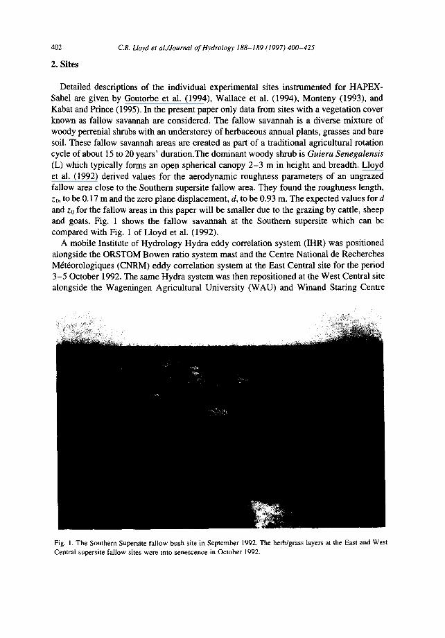
Detailed descriptions of the individual experimental sites instrumented for HAPEX- Sahel are given by Goutorbe et al. (1994), Wallace et al. (1994), Monteny (1993), and Kabat and Prince (1995). In the present paper only data from sites with a vegetation cover known as fallow savannah are considered. The fallow savannah is a diverse mixture of woody perrenial shrubs with an understorey of herbaceous annual plants, grasses and bare soil. These fallow savannah areas are created as part of a traditional agricultural rotation cycle of about 15 to 20 years' duration.The dominant woody shrub is Guiera Senegalensis (L) which typically forms an open spherical canopy 2-3 m in height and breadth. Lloyd et al. (1992) derived values for the aerodynamic roughness parameters of an ungrazed fallow area close to the Southern supersite fallow area. They found the roughness length, z0, to be 0.17 m and the zero plane displacement, d, to be 0.93 m. The expected values for d and z0 for the fallow areas in this paper will be smaller due to the grazing by cattle, sheep and goats. Fig. 1 shows the fallow savannah at the Southern supersite which can be compared with Fig. 1 of Lloyd et al. (1992).

A mobile Institute of Hydrology Hydra eddy correlation system (IHR) was positioned alongside the ORSTOM Bowen ratio system mast and the Centre National de Recherches M&~orologiques (CNRM) eddy correlation system at the East Central site for the period 3-5 October 1992. The same Hydra system was then repositioned at the West Central site alongside the Wageningen Agricultural University (WAU) and Winand Staring Centre

Fig. 1. The Southern Supersite fallow bush site in September 1992. The herb/grass layers at the East and West Central supersite fallow sites were into senescence in October 1992.

C.R. Lloyd et al./Journal of Hydrology 188-189 (1997) 400-425 403

(WSC) eddy correlation systems for the period 7-10 October 1992. The comparison period for the Southern supersite was 5 -9 September 1992. A comparison time closer to the other two sites was not possible as the mobile Hydra was deployed at a fourth site in the HAPEX-Sahel square during the period 10 September-2 October 1992. At the Southern supersite, the mobile Hydra was positioned alongside the University of Reading (UoR) eddy correlation system and another IH Hydra system (IHS) which was resident at the Southern supersite for the whole of HAPEX-Sahel. The comparison at the Southern supersite took place over a relatively wet soil surface at a time when the grass/herb vegetation cover was actively growing. These conditions meant that the comparison took place in neutral or near-neutral conditions. In contrast, the East and West supersite comparisons occurred after the seasonal rains had ceased, the soil was drying, the grass/ herb cover was senescing and the surface layer was becoming more unstable. This differ- ence in conditions had repercussions that are illustrated and commented upon later in the paper. The distances between measurement systems at each of the sites was about 15 m.

3. Instrumental details

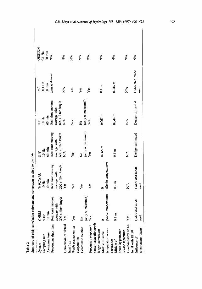
Table 1 lists the position of the fallow savannah sites plus the main physical character- istics of the measurement systems relevant to the present study, and Table 2 lists the eddy correlation software and corrections applied to the data.

The eddy correlation software used by each group was particular to their own system but the underlying routines and corrections were taken from published work. Errors due to a misalignment of the sonic anemometer structure with respect to the local mean streamlines can be removed by the use of a 3-D coordinate rotation of the mean wind vector and of the stress tensor, a method originally proposed by Wesely (1970) and later refined by McMillen (1988). In practice, any rotation should be limited to 10 degrees.

Webb et al. (1980) have shown that even over homogeneous flat terrain, the existence of a vertical flux of sensible heat generates a vertical velocity, which is a consequence of preserving mass conservation. A good overview of the effect of the Webb correction on H20 (and CO2) fluxes is given by Leuning and Moncrieff (1990). The Webb correction is generally of the order of 2-3% for closed-path sensors (e.g. LiCor 6262, Li-Cor Inc, Lincoln, Nebraska, USA) while for open-path systems (Krypton KH20, Campbell Scien- tific, Shepshed, UK and the IH sensor, Institute of Hydrology, Wallingford, UK) it may amount to several tens of per cent depending on the magnitude of the Bowen ratio. The mobile IH Hydra Webb corrections never exceeded 15% (West Central site) and typically had a maximum of 10% and 7% at the East Central and Southern sites respectively. The correction also needs to be applied to the sensible heat flux (Webb et al., 1980), but its effect is much less.

The correction for limited frequency response of the sensors due to finite time constants, path length averaging, lateral and longitudinal sensor separation, damping of the H20 fluctuations in the sampling tubes, and frequency response of the data acquisition system, follow the work of Moore (1986). He calculated transfer functions for these "flux-loss" corrections based on spectral and cospectral functions derived from the Kansas and

404 C.R. Lloyd et al./Journal of Hydrology 188-189 (1997) 400-425

6

o

0

" 0

©

g~

"~ ,o m u,l

._ ~ ~,

E ~ ~ ~ z ~ ~ o - - " o

{ -

• ~ - ~ ~ .~ -~

0

8

z ~. ~

< ' a ~ . ~

O

_ ~ = ~

E

" o

Z ~ ~, ~ ' ~ O ~

¢-,I

t.L/

~.~ o~ ~ i~ o~ I

~-.~ ~ f ~ -- f ~ ,

~ - - ~ , ~ E o ~

"Z

• ~- 8. ' , , ~ ¢ -o . ,-,

o o

1-

C.R, Lloyd et al./Journal of Hydrology 188-189 (1997) 400-425 405

o

E 6

£

6

o ~.~

.8 ~~ ~

~ 6 E " - - 0 3 0

.~ ~=

= .~_ ~ .

~ g 6

g #

~ -

0 E

E E

o

0 . ~ ._ ..~.- ~ °-°!~

406 C.R. Lloyd et aL/Journal of Hydrology 188-189 (1997) 400-425

Minnesota experiments of Kaimal et al. (1972), Kaimal et al. (1976). In the system arrangements used in this paper, the major flux loss occurs through sensor separation. Previous analysis of the Hydra system has shown that a sensor separation of 0.5 m would produce an 8% underestimation of the flux.

The Krypton KH20 hygrometer is sensitive to oxygen density fluctuations (Tanner et al., 1993) which causes a contamination of the latent heat flux by the sensible heat flux and has been corrected for. Representative values of the correction to the evaporation flux are of the order of 10%, which is significant for moderate Bowen ratios.

The measurement of virtual heat flux obtained from the sonic anemometer measure- ments of vertical wind speed and virtual temperature requires correction for the effect of humidity. The correction follows the work of Kaimal and Gaynor (1991) and Schotanus et al. (1983) and typically amounts to 10% of the sensible heat flux.

Flow distortion due to the influence of support structures and the sensors themselves can degrade the turbulent velocity measurements (Wyngaard, 1988). The support effect was minimised by systems being placed on top of thin masts. The Solent sonic anemometer (Gill Instruments, Southampton, UK) allows real-time correction and calibration of the three wind components for the effects of structure and transducers. Typically, when a strut is upwind of the measurement area, the horizontal wind will need to be corrected by 7%. The Hydra has a single vertical sonic, which minimises the problem. The effect of the structure on the calibration and functioning of the Hydra was investigated using a wind tunnel by Shuttleworth et al. (1988) and amounted to no more than 5% for a 330 ° accep- tance angle.

4. Comparison of individual system surface flux measurements

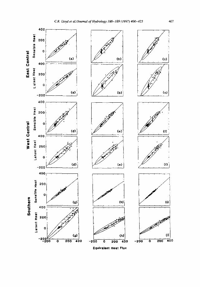
The measurement of surface fluxes by eddy correlation sensors is a non-linear process, with flux sources, both upstream and across-stream, contributing more or less flux to the measurement depending upon their position upwind of the sensor. The application of diffusion theory (e.g. Gash, 1986, Schmid and Oke, 1990) can identify an area upwind of the sensor, from within which a percentage of the flux emanates. This is termed the flux footprint. The areal extent of this footprint, and the point source strengths within this footprint contributing to the measured flux, dynamically change with wind direction, roughness length and atmospheric stability. In heterogeneous terrain where surface cover and soil moisture may vary from place to place, short-term flux measurements at one position may not agree with similar measurements at an adjacent position because of their different footprints. This effect was shown by Lloyd (1995).

The surface flux measurements recorded by individual eddy correlation systems at a common fallow bush site will be at variance through three major effects; the true sampling

Fig. 2. Flux regression scatterplots, regression line and 90% bivariate ellipses for combinations of instrument system Sensible and Latent heat fluxes at the East Central, West Central and Southern sites. (a), CNRM vs. IHR; (b), ORSTOM vs. IHR, (c), ORSTOM vs. CNRM; (d), WAU vs. IHR, (e), WSC vs. IHR; (f), WSC vs. WAU; (g), IHS vs. IHR; (h), UoR vs. IHR, (i), UoR vs. IHS. The second named system is on the abscissa. Flux values are in W m -2.

C.R. Lloyd et al./Journal of Hydrology 188-189 (1997) 400-425 407

4 0 0

2 0 0

m ~ 0 m

c @ 0 4 0 0

m ~ 2 0 0 w .

c O

= 0 J

- 2 0 0

J (a)

~c) 4 0 0

2 0 0

G )

. , ~ o

o U 4 0 0

: r 2 0 0

c

,,_1

- 2 0 0

4 0 0

2 0 0 -t-

J ~

"~ 0

E}, @ ,,c

4 0 0 3 O

:~ 2 0 0

c @

0 . =

- J .

- 2 0 0 / , , - 2 0 0 0

J (g)

2 0 0 4 0 0

(h)

f (h)

, J , h i

- 2 0 0 0 2 0 0 4 0 0

i i = i i

i i , J . ,

J (I) i i i , i

- 2 0 0 0 2 0 0 4 0 0

Equ i va len t Hea t F lux

408 C.R. Lloyd et al./Journal of Hydrology 188-189 (1997) 400-425

of different flux entities due to spatial heterogeneity, the high or low frequency flux loss through restricted data sampling, and errors caused by sensors failing to measure correctly, through calibration drift and design faults. The variability in the comparison of surface fluxes in the sections below is composed of all these factors.

The short comparison periods (3 days) for these measurements and the similar conditions during these periods will limit the effect of calibration drift and will tend to create constant discrepancies due to sensor design faults. The effect of spatial variability upon the discrepancy between individual system measurements will become progressively weaker as these measurements are summed over longer periods due to the "averaging out" of the surface inhomogeneity by wind direction and flux footprint changes. From the above, it would seem that only long-term flux averages should be used to characterise the possible confidence limits to flux measurements at any of the HAPEX-Sahel sites. However, investigation of diurnal effects will require short-period data and these data will have different confidence limits mainly due to the effects of spatial variability. The analysis below intercompares the different system measurements over three days of hourly measurements and over the combined average of these three days.

4.1. Pairwise comparisons: linear regressions

At each of the three sites, regressions of hourly values of latent and sensible heat fluxes were carried out for each pairing. Fig. 2 shows these regressions at each of the three sites. The regression plots also show the 95% Gaussian bivariate confidence interval based around the sample means of the two variates. This envelope, although strictly not applic- able to these distributions, is analogous to the sample standard deviation for a univariate population and usefully highlights the spread of the regression. Additional statistical analyses were performed on these paired systems and the results are shown in Table 3. For each pairing, the slope and intercept were tested for any significant difference from unity and zero respectively. The relative error is the difference between the total fluxes measured by the dependent and independent variables normalised by the average of the totals from the two measurement systems. In homogeneous terrain, any large deviation in the relative error from zero would have indicated that one or other of the systems was not working correctly. In heterogeneous terrain, the situation is not so obvious. The standard error of the estimate provides an estimate of the variance about the regression and is used to create the 95% prediction intervals in the final column. The prediction intervals, ana- logous to confidence intervals, relate to single values rather than a sample mean and have been computed not at the mean regression coordinates but at the maximum flux values encountered at each site. Using such a statistical measure at that value provides a better idea of the possible variability for midday hourly fluxes. Some general conclusions are discussed in the next sections.

4.2. Sensible heat flux 2-system comparisons

At the EC site, the best correlation between systems, indicated by R 2, relative and standard error and confidence interval in Table 3, but also visually by the narrowness of the ellipse in Fig. 2(a) is between CNRM and IHR. Inspection of the regression graph

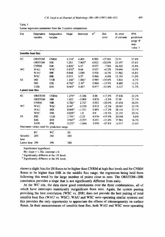
C.R. Lloyd et al./Jourr~l of Hydrology 188-189 (1997) 400-425

Table 3 Linear regression parameters from the 2-system comparisons

409

Site Dependent Independent Slope Intercept R 2 Rel. variable variable error

St. error of estimate

95% prediction range @ max. value +_

Sensible heat flux

EC ORSTOM CNRM 1.218 ~ 4.405 0.903 +27.6% ORSTOM IHR 1.051 7.965 b 0.922 +20.0% CNRM IHR 0.828 ~ 4.47 0.937 -7.8%

WC WAU WSC 0.932 b 0.64 0.937 +0.2% WAU IHR 0.948 2.089 0.926 -6.5% WSC IHR 0.975 0.57 0.966 -6.8%

SS IHS UOR 1.166 ~ 1.884 b 0.985 +25.6% IHS IHR 0.782 ~ 2.34 b 0.966 -15.9% UOR IHR 0.669" 0.457 0.977 -41.0%

Latent heat flux

25.93 23.197 16.302 19.694 21.962 15.193 5.844 8.609 6.227

17.6% 17.6% 15.8% 15.0% 16.8% 11.0% 6.3%

13.2% 11.3%

EC ORSTOM CNRM 1.274 ~ -5.388 0.88 +17.5% ORSTOM IHR 1.023 -3.909 0.878 -2.5% CNRM IHR 0.784 a 2.727 0.952 -20.0%

WC WAU WSC 0.94 b ~3.529 0.933 +2.3% WAU IHR 0.868 ~ -I.531 0.893 -17.2% WSC IHR 0.829' 1.9 0.9 -19.5%

SS IHS UOR 1.791 ~ -2.25 0.976 +57.9% IHS IHR 0.945 b -5.935 0.951 -11.0% UOR IHR 0.525 ~ -1.846 0.956 -67.8%

Maximum values used for prediction range

37.836 37.98 17.654 20.967 28.141 25.255 20.048 27.961 14.977

22.2% 27.1% 16.0% 15.1% 23.1% 20.3%

6.6% 16.3% 15.6%

EC WC SS Sensible 260 260 160 heat Latent heat 290 290 380

Significance hypotheses Ho: slope = 1 ; Ho: intercept = 0. Significantly different at the I% level.

b Significantly different at the 5% level.

shows a s l igh t b ias for IH f luxes to b e h i g h e r t h a n C N R M at h i g h flux levels and for C N R M

fluxes to be h i g h e r than I H R in the m i d d l e flux range , the r eg res s ion be ing he ld f r o m

fo l l owing th is t r end by the l a rge n u m b e r o f po in t s c lose to zero. The O R S T O M - I H R

cor re l a t ion p r o v i d e s a s lope t ha t is no t s ign i f i can t ly d i f fe rent f r o m unity.

At the W C site, the da ta s h o w good co r r e l a t i ons ove r the three c o m b i n a t i o n s , all o f

w h i c h h a v e in te rcep t s s t a t i s t i ca l ly i n s ign i f i c an t f r o m zero. Aga in , the sys t em pa i r ing

p r o v i d i n g the bes t co r r e l a t i on ( W S C vs. IHR) does not p rov ide the bes t pa i r ing o f total

sens ib le hea t flux ( W A U vs. W S C ) . W A U a n d W S C were opera t ing s imi la r sys t ems and

this p r o v i d e s the on ly o p p o r t u n i t y to app rec i a t e the effects o f i n h o m o g e n e i t y on sur face

fluxes. In t he i r m e a s u r e m e n t s o f s ens ib l e hea t flux, bo th W A U and W S C were opera t ing

410 C.R. Lloyd et aL/Journal of Hydrology 188-189 (1997) 400-425

Solent sonic anemometers with fine wire thermocouples and similar software. The major differences as shown in Table 1 were differences in sampling rate, a difference of 0.45 m in measurement height and a sensor separation differing by 17 ram. The observed differ- ences in the regression analysis are most probably due to a combination of the effects of these differences together with the effects due to spatial inhomogeneity. By considering the transfer functions evaluated by Moore (1986) for assessing the flux loss in eddy correlation systems due to sampling rate and sensor separation, the expected difference between the WAU and WSC sensible heat fluxes due to the above disparity in sampling rate and sensor separation amounts to less than 1%. This implies that the remaining differences are due to the systems sampling from different flux footprints which result from their spatial separation and difference in measurement height. At the WC site, the measurement systems' long-term summation of fluxes (where the effects of different source footprints are averaged out) are highly comparable. However, for hourly average values, where the difference between flux footprints becomes more important, the correla- tion is not as good.

At the Southern site, all three systems provide good correlations and poor flux estimates. The good correlations are probably due to the timing of the intercomparison, at the beginning of September and four days after a five-day period of rainfall totalling 68 mm. The grass/herb layer was actively growing and the disparity between bare soil, grass/herbs and bush fluxes was at a minimum. The poor agreement between the sensible heat flux estimates from the two IH Hydras may be due to the marked difference in height (9.5 m and 4.5 m). A field comparison (without recalibration of the instruments) between the two Hydras in August 1993 at Wallingford did not produce this sensible heat flux difference.

5. Latent heat flux 2-system comparisons

Surprisingly, because the measurement of evaporation is still regarded as more difficult than that of sensible heat, the regressions and overall variability for latent heat are gen- erally no worse than for sensible heat.

At the East Central Site, the tightest regression was between CNRM and IH (R 2 = 0.952) but the ORSTOM-IH pairing came closest to agreeing the size of the total flux produced during the three days (relative error of 2.4%) and produced a slope not significantly different from unity. The IH system appears to be overestimating evaporation compared to the CNRM system and the CNRM system is underestimating evaporation when com- pared to the ORSTOM measurements.

At the West Central Site, the WAU-WSC pairing provided both the best regression and the closest agreement on total flux. The IH system again appears to be overestimating evaporation. WAU and WSC were operating different hygrometers and the veiled possi- bility of similar but erroneous fluxes through operating similar systems, as for the sensible heat, does not hold in this case.

At the Southern Site, the regressions are the best of all three sites. The roving IH system appears to be overestimating evaporation compared to the "resident" IH Hydra, but again in field tests at Wallingford the following summer, no systematic difference was found.

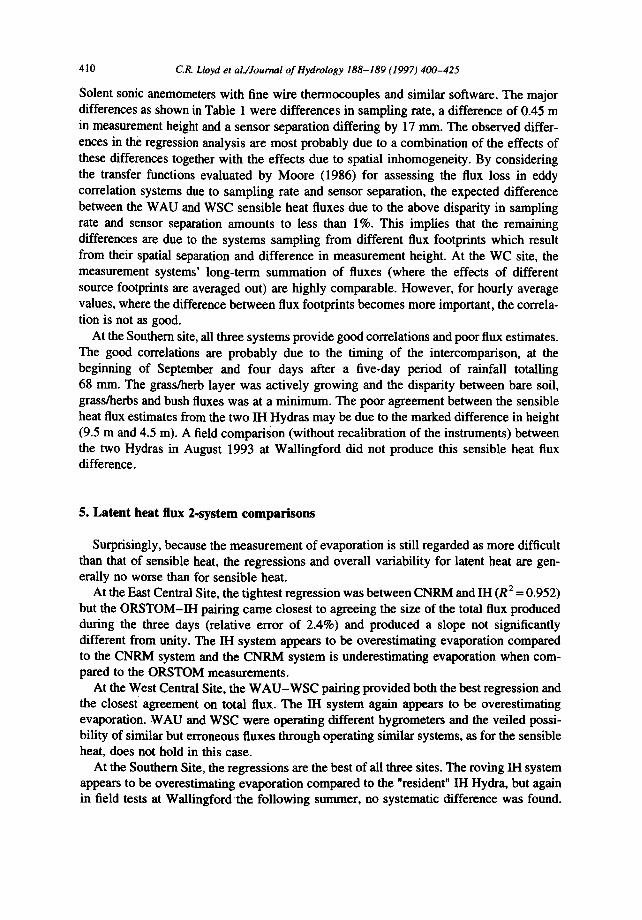
C.R. Lloyd et al./Journal of Hydrology 188-189 (1997) 400-425 411

Tests carried out by the University of Reading, both during and after the IOP, indicated that the calibration of their Ophir IR-2000 Hygrometer was irretrievably wrong. Despite this, the instrument has produced the best correlations of any pairing (R 2 = 0.976 and R 2 = 0.956) against both of the Hydras. This may indicate that the data may be recoverable, if required, by applying a field calibration.

The validation of land-surface models will variously require data averaged over periods from minutes to periods of many days. These time averages will usually consist of many data points. However, for each of these time averages, there will usually be no more than a few spatial replicates. A prediction interval provides a measure of the inherent variability in a single measurement, in this case a single hourly average measurement. For example, at the West Central Site, a 15% prediction interval about a regression predicted mean for the WAU-WSC pairing, indicates that for a midday sensible heat flux of 260 W m -2 measured by the WSC system during a time averaging period, it is expected that the WAU system will measure 243 W m -2 (according to the regression line), but that one must accept, with 95% confidence, as equally valid any measurement by the WAU system between 207 and 279 W m -2.

O

. o

gu

300

200

100

500

,d

East Cemral West Central Southern

I i i i i

- 2

1.5 o

* 1

0.5 i i h i

_o r ~

.,00 t t

200 2 o

'~ i 1.5 "0" • i

• ~- • i . . 1

~, 0.5

ORSv|HR W A U Y W S G WSCIIflR IHSIIHM

Instrument Systems

Fig. 3. Sensible and latent heat prediction ranges and gradients from the pairwise regression analysis at the three sites.

412 C.R. Lloyd et al./Journal of Hydrology 188-189 (1997) 400-425

The regression slopes and the prediction ranges for the results tabulated in Table 3 are shown in Fig. 3(a). The prediction ranges are centred on typical midday flux values at each site during the intercomparison periods.

At the West Central site, and using the WAU-WSC pairing in this example, the ranges of confidence in the measurements of sensible and latent heat are similar. This is probably because the latent and sensible heat fluxes at this site during the intercomparison were similar in size. The expected value for the WAU system if the WSC system measures 300 W m -2 is 281 W m -2 but one would only expect to be wrong 5% of the time if one predicted it would be somewhere between 237 and 325 W m -2. Fig. 3(b) shows the regression slopes and prediction ranges for the latent heat fluxes at the three sites. Again the prediction ranges are centred on typical midday latent heat fluxes during the intercomparison periods.

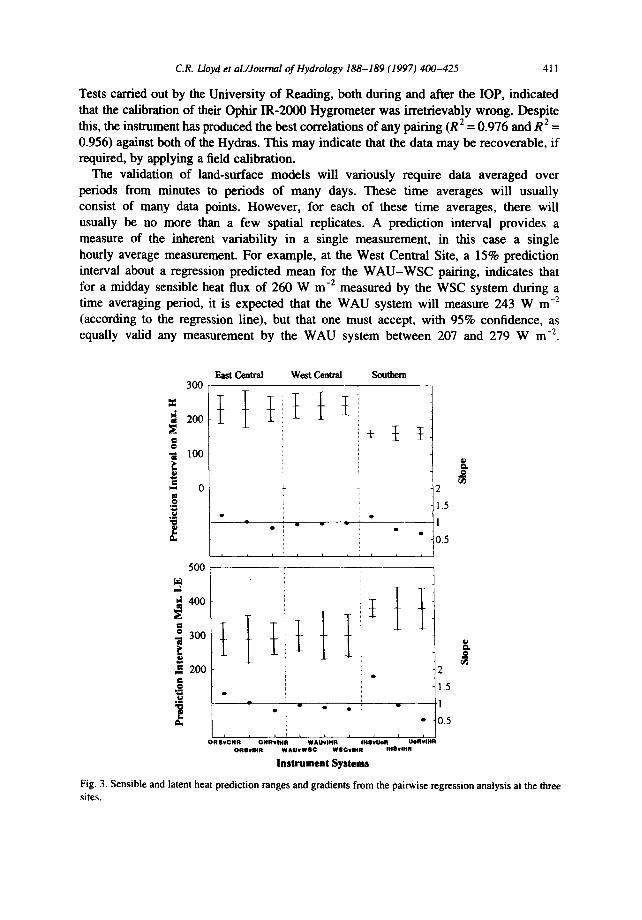
5.1. Pairwise comparisons: difference scheme

It may be argued that ordinary linear regression is strictly inappropriate in assessing the performance of the systems. The measurements providing the independent variable are themselves subject to error which should be included in the regression model and equal weight is given to both small and large flux measurements.

Therefore the differences between paired hourly measurements were examined. These differences were normalised by the average of their sum, i.e.

%Variation= (FluxA-Flux//) x 100% (1) 1 ~(FluxA + FluxB)

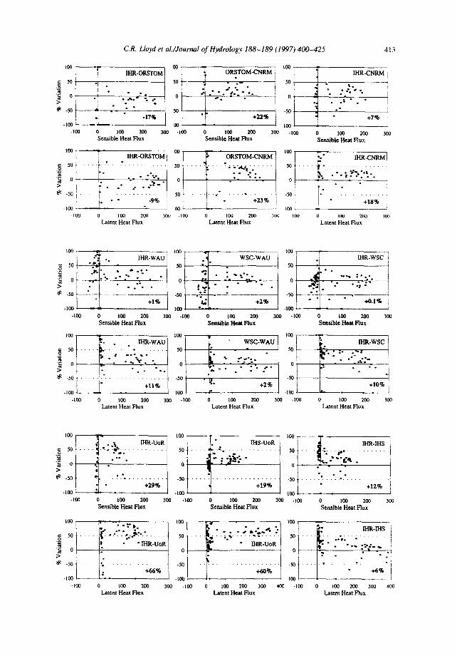
The results of this comparison are shown in Fig. 4 for the East, West and Southern sites. The x-axis is the average flux from the system-pair, i.e. the denominator in Eq. (1). Occasionally, and usually for low flux values, exceedingly large absolute ratios can occur. In the figures, a capping limit of 100% is placed on the ratios. In the analysis, the ratios which are capped are excluded. From the figures it is apparent that percentage variation decreases as flux values increase. This is probably due to the measurement systems performing better in unstable conditions than in stable or night-time conditions when system configuration becomes more important and the configuration corrections to the flux may dominate.

A value for the mean flux difference for each system pairing was achieved by averaging weighted flux differences according to the following formula

Mean System-pai r % difference = FluxA + FluxB £ 2

(2)

Fig. 4. Normalised sensible and latent heat differences between system pairs at the East Central site, West Central and Southern sites.

C.R. L loyd et a l . / Journa l o f H y d r o l o g y 1 8 8 - 1 8 9 (1997) 4 0 0 - 4 2 5 4 1 3

LOO . . . . iV

I -~ so "I

-50 .

-too ! -leo 0

e e l '~' 100T [ H R - O T T O M I .~ : ~ T O M - C N R M , i , , . . . IHR-CNRM %

. . , . . , . . . o -~'" " "" o 5 " '

- ; " - 1 7 - 5 0 + 7 %

-- leo . . . . leO 200 300 -leO 0 tOO 200 300 -leO 0 tOO 200 300

Sensible Heat Flux Sensible Heat Flux Sensible Heat Flux

• 50 . . . . . . . . . . . . . . . . . 50 T + . +i . . . . . . . . . . . . . . . . 50 ~ .

I - . .1 "=~ - • " $ - " + z

O % - " i - ' : . : ' . °1 ~- -- . - - : - - I o -50 -• . . . . . . . . . . . . 50

; L • " -9% + - ,oo {" + oo i L ; ,oa ~.

-I0~ O I00 21)1) 3011 -llX] 0 I(X) 2L~} 3IX) -ILK} 11 11141 21)0 31JO

Latent Heat Flux Latent Heat Flux Latent Heat Flux

i0o :". IHR-WAU ~oo o• so ".% 50

• ~ .- • . .~..

o . . . " ' : 2 :; o • o

40 . . . . -5<:,

+ 1 %

-tOO -- IOO -I00 0 leO 200 300 -too

Sensible Heat Flux

1 130 I{30 F i b IHR-WAU 1 , ' W S C - W A U o•

=- = so . . . . . . . . . . . . . so . .:._:.

"~ ~ ' ' * " " ' " i" ." " ' - ' ~ , " o "-" "~ 0 ; . , . . . . . , . - w. o o

- 5 0 -SO . ~ + 1 1 % " + 2 %

-I00 - - - - tO0 -leo 0 10<3 200 300 -too 0 too 200

Latent Heat Flux

1 0 0 r ~ W S C - W A U IHR-WSC i

" " 50 • . .

.~.¢. ~ "." . . . . . : - - - - . - ~ " - - - 5 0 " "

t ~ + 2 % " +0 .1% . . . . . . -leo

0 leO 200 300 .1110 0 IOO 200 300 Sensible Heat Flux Sensible Heat Flux

~. IHR-WSC

I~, • ;- • "~...':.

I +10% • tOo - - - - - '~ ' , ' - - --~ . . . . . J

300 -100 0 tOO 200 300 Latent Heat Flux Latent Heat Flux

loo loo

g 50 I-" ." "~'. IHR-UoR t . " - -. , ; . 50 '- -"-.- -

-~ o ,~ o -: "J~':"

.SO a. • • .SO . . . ' +

• " +29%

-tOO -tOO J'

-tOo o 100 200 300 -leo Sensible Heat Flux

l e o ,.see, :, 5 " ~ " " " " i* . . . .

IHR-IHS

-50 - - -°- ~ . . . . . . . .

too ~ • . + 0 leo 200 300 -too 0 1{30 200 300

Sensible Heat Flux Sensible Heat Flux

too ~. - ' : . ' . ' , . } 'oo e . . '°°1 ~ ~ . ~ s I

:i ,+ - + " +I . . . . . . . . . . . . + g 5 - ~ . . . . ; - . -

:~ ~ " IHR-UoR . - . . . ~ . e . . o . o . ~ . , . .

-50 k

+12 : . . . . +6,,t +,o,+ +°t I ' + , i -I00 0 100 200 300 ,1(30 0 100 200 300 400 -leo 0 t i l l? 200 300 400

Latent Heat Flux Latent Heat Flux Latent Heat Flax

414 CR. Lloyd et aL/Journal of Hydrology 188-189 (1997) 400-425

These values are indicated in the bottom fight hand corner of each graph. A comparison can now be made between the results from the pairwise regression analysis and the above difference scheme. Generally the difference scheme gives system differences that are smaller than those produced by the regression lines. It is probably most appropriate to use the difference scheme to assess period overall system flux differences. However, the method does not convey much information about the variability of the individual measure- ments about these mean values.

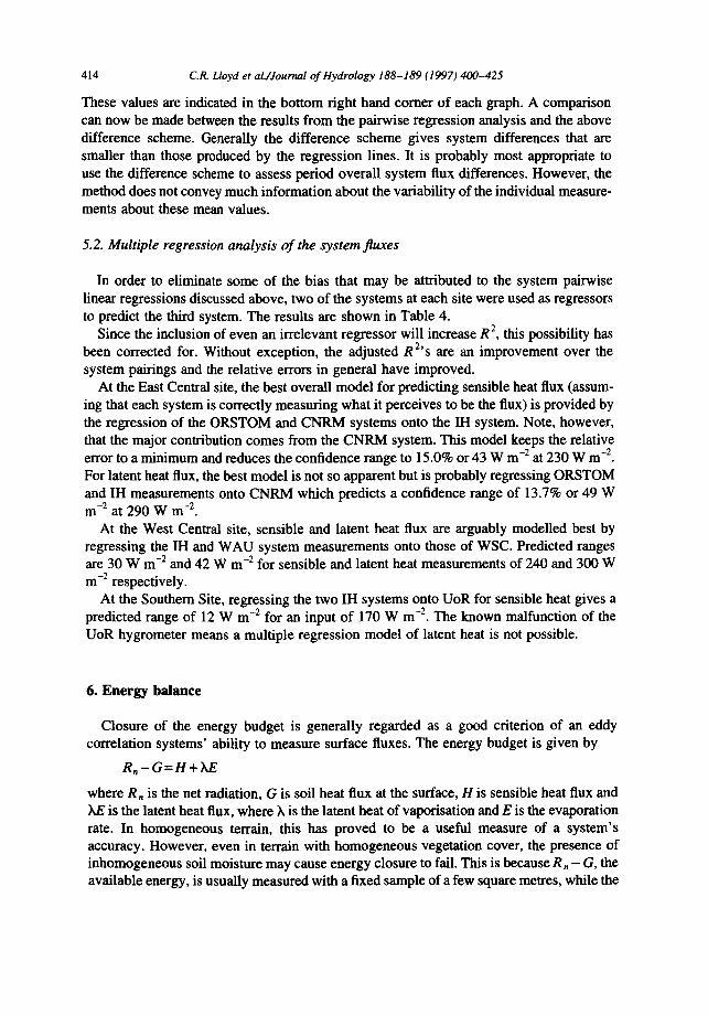
5.2. Multiple regression analysis o f the system fluxes

In order to eliminate some of the bias that may be attributed to the system pairwise linear regressions discussed above, two of the systems at each site were used as regressors to predict the third system. The results are shown in Table 4.

Since the inclusion of even an irrelevant regressor will increase R E , this possibility has been corrected for. Without exception, the adjusted R 2 ' s a re an improvement over the system pairings and the relative errors in general have improved.

At the East Central site, the best overall model for predicting sensible heat flux (assum- ing that each system is correctly measuring what it perceives to be the flux) is provided by the regression of the ORSTOM and CNRM systems onto the IH system. Note, however, that the major contribution comes from the CNRM system. This model keeps the relative error to a minimum and reduces the confidence range to 15.0% or 43 W m -2 at 230 W m -2. For latent heat flux, the best model is not so apparent but is probably regressing ORSTOM and IH measurements onto CNRM which predicts a confidence range of 13.7% or 49 W m -2 at 290 W m -2.

At the West Central site, sensible and latent heat flux are arguably modelled best by regressing the IH and WAU system measurements onto those of WSC. Predicted ranges are 30 W m -2 and 42 W m -2 for sensible and latent heat measurements of 240 and 300 W m -2 respectively.

At the Southern Site, regressing the two IH systems onto UoR for sensible heat gives a predicted range of 12 W m -2 for an input of 170 W m -2. The known malfunction of the UoR hygrometer means a multiple regression model of latent heat is not possible.

6. Energy balance

Closure of the energy budget is generally regarded as a good criterion of an eddy correlation systems' ability to measure surface fluxes. The energy budget is given by

R ~ - G = H + KE

where Rn is the net radiation, G is soil heat flux at the surface, H is sensible heat flux and KE is the latent heat flux, where ), is the latent heat of vapofisation and E is the evaporation rate. In homogeneous terrain, this has proved to be a useful measure of a system's accuracy. However, even in terrain with homogeneous vegetation cover, the presence of inhomogeneous soil moisture may cause energy closure to fail. This is because Rn - G, the available energy, is usually measured with a fixed sample of a few square metres, while the

C.R. Lloyd et al./Journal of Hydrology 188-189 (1997) 400-425 415

. ,rl-

d,@ +1

~,-.= E

=

g E

~.~

J ~

. . . . ~ m ~ . -- .

~ . ~ ~

• . ~ , . . ~ . ~ . ~ . R

. . ~ ~ o ~

~_~

i

- ' : - ~ - ~

E

416 C.R. Lloyd et al./Journal of Hydrology 188-189 (1997) 400-425

fluxes are a composite measurement from a varying upwind footprint of heat and water vapour sources. If the fluxes are emanating from a surface area that has different heat and moisture balances and hence a different available energy to that where Rn and G are being measured, then energy closure will fail.

In heterogeneous terrain, the situation is still more complicated. Each different surface within the mosaic has its own available energy. To measure the available energy corre- sponding to the measured fluxes successfully, a net radiometer will need to be placed at such a height that the measurement contains, not just the contributions from all the surface types, but contributions in proportion to the larger scale area from within which the surface fluxes are emanating. As the height of the net radiometer increases, the measurement is degraded by longwave losses in the air layer between the surface and the measurement height.

An alternative method is to measure the net radiation and soil heat flux individually for each of the component surface types and then to weight the resultant measurements according to photographic or some similar survey of the area upwind of the flux measure- ments. While this reduces any errors incurred through flux loss, it cannot account for the varying shadowing effect of each surface type on the others. For mosaic patterns of the same height, this need not be a problem but in fallow savannah where the composite surfaces consist of bushes shading grass and herbs which in turn shade bare soil, shading may have some effect.

Soil heat flux is commonly either measured close to the surface or at some depth with a correction for the heat storage in the soil layer above the heat flux plate. The latter method requires some knowledge of the soil thermal conductivity, which is difficult to assess and can be highly variable in many soils, and a temperature gradient measurement at succes- sive time intervals. Surface soil heat flux may give erroneous results where the level at which soil moisture is evaporating is below that of the heat flux plate. The heat flux plate measurement is then being contaminated by the heat of vaporisation. Generally, in a soil that is not recently wetted and when daily mean temperatures are not changing greatly, soil heat flux over the 24 hours is close to zero.

Therefore, the practice of assuming the combination of net radiation and soil heat flux to be a good estimate of available energy, and hence a good test of the measurements of sensible and latent heat flux, is not as applicable in heterogeneous terrain as it is in homogeneous terrain.

Net radiation and soil heat flux were measured at each of the sites in this study but without the application of a common measurement strategy. At the East central site, net radiation was measured at 11.5 m by ORSTOM and at 8 m by CNRM. Soil heat flux was measured by one soil heat flux plate at a depth of 20 mm by ORSTOM. At the West Central site, net radiation was measured at 10 m and soil heat flux by 4 plates at depths from 50 mm to 400 mm by WSC. At the Southern site, net radiation was measured separately over bush and grass/herb substrates and compositely from 4.7 m by IH. Net radiation was also measured at 3 m by UoR. Soil heat flux was measured separately beneath the bush and grass/herb surfaces by IH, 6 plates at 100 mm beneath a grass/ herb layer and 3 plates at 100 mm beneath a bush. The measurements from these two sets of plates were averaged separately and then combined in the ratio of herb/grass to bush areal coverage. UoR also measured soil heat flux by 4 plates at a depth of 50 mm.

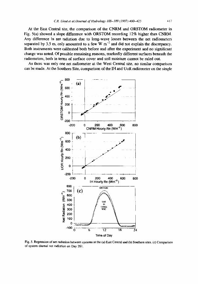
C.R. Lloyd et al.IJournal of ttydrology 188-189 (1997) 400-425 417

At the East Central site, the compar ison of the CNRM and ORSTOM radiometer in Fig. 5(a) showed a slope difference with O R S T O M recording 12% higher than CNRM. Any difference in net radiation due to long-wave losses between the net radiometers separated by 3.5 m, only amounted to a few W m -2 and did not explain the discrepancy. Both instruments were calibrated both before and after the experiment and no significant change was noted. Of possible remaining reasons, markedly different surfaces beneath the radiometers, both in terms of surface cover and soil moisture cannot be ruled out.

As there was only one net radiometer at the West Central site, no similar comparison can be made. At the Southern Site, comparison of the IH and UoR radiometer on the single

A 8 0 0 ,

'E ~ 600 . . . . . . . . . . . . . . . . . . . . . . . . . c ¢ r

~, 400

O I 200

~ 0 ffl

0 -200

-200 0 200 400 600 800 CNRM Hourly Rn (Wm -2 )

8°°! (b) ! ?

200 -1- ¢r'

° t -200 , , L b , -200 200 400 600 800

IH Houdy Rn (Win "2) 800

ORS'TOM

700

? 600

~ 5 0 0

~ 400

300

200

100

0

- 1 O0 0 6 12 18 24

Time of Day

Fig. 5. Regression of net radiation between systems at the (a) East Central and (b) Southern sites. (c) Comparison of system diurnal net radiation on Day 261.

418 C.R. Lloyd et al./Journal of Hydrology 188-189 (1997) 400-425

East Central

-2011 . . . . 12 12 12 g00

t West Central 6 0 0 . . . . . . . . . . . . . . . . . . . . . . . . . . . . . . . . .

.~ 400

200

'~ 400

.~ 200 m

-200 L 1'2 12 1'2 1'2

800 t Southern

~" 600 i i i ! ~ ~ ~ ! ~ , ~ ' ~ 400

200 t

0 ~ ~ 7 1 2 - - 1 2 -200 1'2 ' 1'2 ' '

Time of Day

Fig. 6. Diurnal net radiation and soil heat flux values at the three fallow sites during the comparison periods. Net radiation is the solid line, soil heat flux is the dotted line.

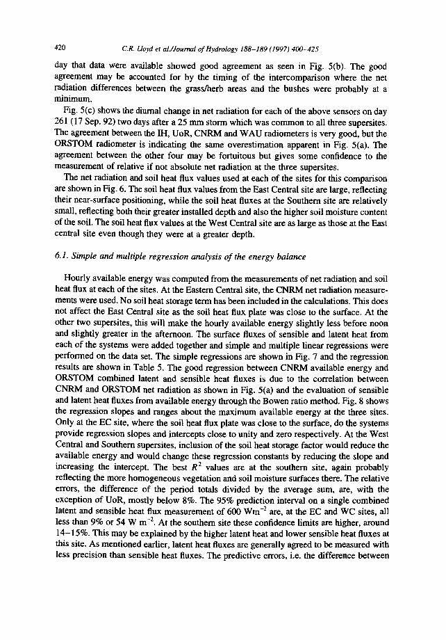
Fig. 7. Regression scatterplots, regression line and 90% bivariate ellipses for system sensible latent heat fluxes (H+LE) and available energy (Rn - G) at the East Central, West Central and Southern sites. Upper group: comparison of system H + LE; (a) CNRM vs. IHR; (b) ORSTOM vs. IHR, (c) ORSTOM vs. CNRM; (d) WAU vs. IHR; (e) WSC vs. IHR; (f) WSC vs. WAU, (g) IHS vs. IHR; (h) UoR vs. IHR; (i) UoR vs. IHS. The second named system is on the abscissa. Lower group: comparison of system H + LE fluxes with site available energy; (a) CNRM, (b) ORSTOM, (c) IHR, vs. CNRM (Rn - G); (d) WAU, (e) WSC, (f) IHR, vs. WSC (Rn - G); (g) IHS, (h) UoR, (i) IHR, vs. IHS (R~ - G).

C.R. Lloyd et al./Journal of Hydrology 188-189 (1997) 400-425 419

6 0 0

~" ~ 300

w o

6 0 0

~ 300

,,J ÷ 0

_e _ . 60o m @

{/) - 300 0

. . . . . . !'

0 3 0 0 6 0 0 0 3 0 0 6 0 0

Sensible ÷ Latent Heat flux (Wnt 2) 0 3 0 0 6 0 0

t . . . . . . - 6 0 0 i ~ '

300

(:)

.,., _ 6 0 0 @

.,., 0 3 0 0

"J 0 4.

$ __= 600

(d) "

° ° e U) ~. 3OO

° ~ S " . . . . c~) I , , , , i h ,

0 300 600

~)

I

0 3 0 0 6 0 0 O " 300 600

Available Energy (Win -2)

420 C.R. Lloyd et aL/Journal of Hydrology 188-189 (1997) 400-425

day that data were available showed good agreement as seen in Fig. 5(b). The good agreement may be accounted for by the timing of the intercomparison where the net radiation differences between the grass/herb areas and the bushes were probably at a minimum.

Fig. 5(c) shows the diurnal change in net radiation for each of the above sensors on day 261 (17 Sep. 92) two days after a 25 mm storm which was common to all three supersites. The agreement between the IH, UoR, CNRM and WAU radiometers is very good, but the ORSTOM radiometer is indicating the same overestimation apparent in Fig. 5(a). The agreement between the other four may be fortuitous but gives some confidence to the measurement of relative if not absolute net radiation at the three supersites.

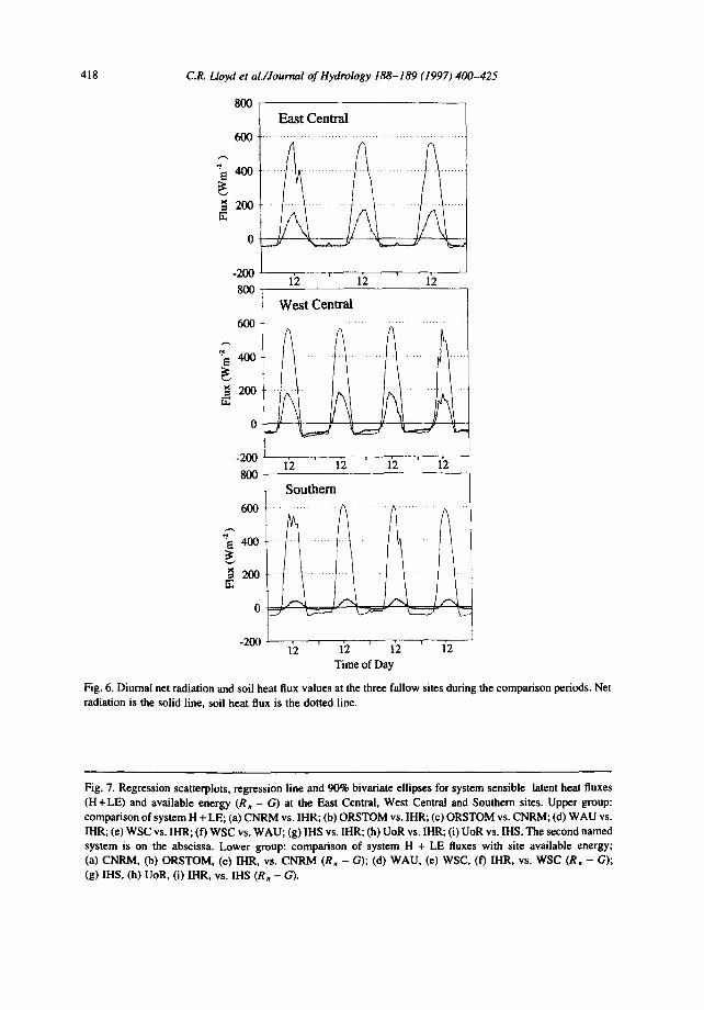
The net radiation and soil heat flux values used at each of the sites for this comparison are shown in Fig. 6. The soil heat flux values from the East Central site are large, reflecting their near-surface positioning, while the soil heat fluxes at the Southern site are relatively small, reflecting both their greater installed depth and also the higher soil moisture content of the soil. The soil heat flux values at the West Central site are as large as those at the East central site even though they were at a greater depth.

6.1. Simple and multiple regression analysis of the energy balance

Hourly available energy was computed from the measurements of net radiation and soil heat flux at each of the sites. At the Eastern Central site, the CNRM net radiation measure- ments were used, No soil heat storage term has been included in the calculations. This does not affect the East Central site as the soil heat flux plate was close to the surface. At the other two supersites, this will make the hourly available energy slightly less before noon and slightly greater in the afternoon. The surface fluxes of sensible and latent heat from each of the systems were added together and simple and multiple linear regressions were performed on the data set. The simple regressions are shown in Fig. 7 and the regression results are shown in Table 5. The good regression between CNRM available energy and ORSTOM combined latent and sensible heat fluxes is due to the correlation between CNRM and ORSTOM net radiation as shown in Fig. 5(a) and the evaluation of sensible and latent heat fluxes from available energy through the Bowen ratio method. Fig. 8 shows the regression slopes and ranges about the maximum available energy at the three sites. Only at the EC site, where the soil heat flux plate was close to the surface, do the systems provide regression slopes and intercepts close to unity and zero respectively. At the West Central and Southern supersites, inclusion of the soil heat storage factor would reduce the available energy and would change these regression constants by reducing the slope and increasing the intercept. The best R 2 values are at the southern site, again probably reflecting the more homogeneous vegetation and soil moisture surfaces there. The relative errors, the difference of the period totals divided by the average sum, are, with the exception of UoR, mostly below 8%. The 95% prediction interval on a single combined latent and sensible heat flux measurement of 600 Wm -2 are, at the EC and WC sites, all less than 9% or 54 W m -2. At the southern site these confidence limits are higher, around 14-15%. This may be explained by the higher latent heat and lower sensible heat fluxes at this site. As mentioned earlier, latent heat fluxes are generally agreed to be measured with less precision than sensible heat fluxes. The predictive errors, i.e. the difference between

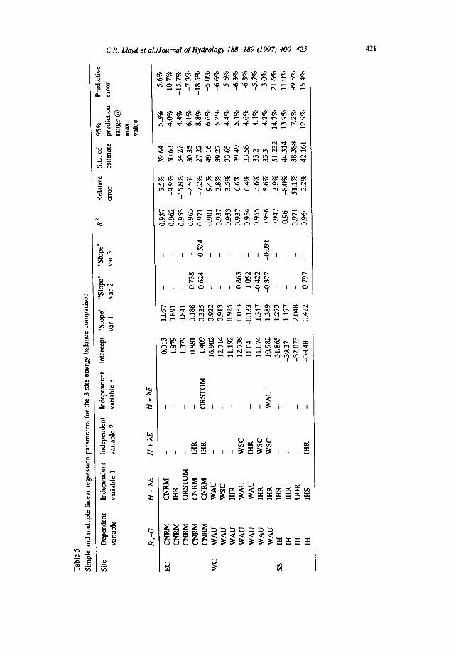
C.R. Lloyd et al./Journal o.f Hydrology 188-189 (1997) 400-425 421

o

¢}

%

m i.,,

~ ~ . =

~.' '~

-F

+

+

II I

I

I I I I ~ I I I I I I ~ I I I I

I I I I

© [--,

i i i i o i i i i i i ~ i i i i

r,.)

422 C.R. Lloyd et al./Journal of Hydrology 188-189 (1997) 400-425

East Central West Central Southern 800

700

g 6oo

500

..~

2

1.5

1

0.5

_o

CNiRM * ORI { tTOM I WSGI , }HSJ t I (HR WAU IHR IHR

Instrument Systems

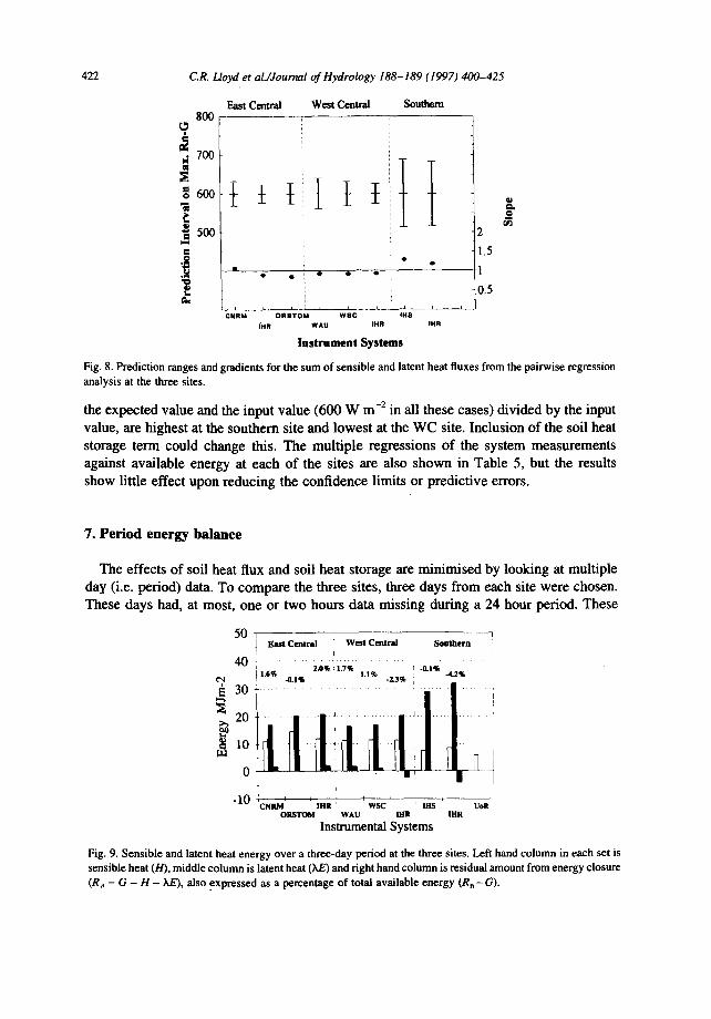
Fig. 8. Prediction ranges and gradients for the sum of sensible and latent heat fluxes from the pairwise regression analysis at the three sites.

the expected value and the input value (600 W m -2 in all these cases) divided by the input value, are highest at the southern site and lowest at the WC site. Inclusion of the soil heat storage term could change this. The multiple regressions of the system measurements against available energy at each of the sites are also shown in Table 5, but the results show little effect upon reducing the confidence limits or predictive errors.

7. Period energy balance

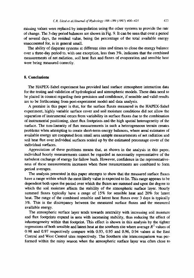
The effects of soil heat flux and soil heat storage are minimised by looking at multiple day (i.e. period) data. To compare the three sites, three days from each site were chosen. These days had, at most, one or two hours data missing during a 24 hour period. These

50 1 L East Central West Cemtral S o u t h e r n i

2.0% 11.7% i l . 6% .01% 1.1% 2.3% -0.1% -4.2%

~ 30 . . . . . . . . . . . . . . . . . . . . . . . .

~ 20 ~ . . . . . . . . .

0 i " ' I i I

-lO ~' mR' wsc ' tm uon ORSTOM WAU mR [HR

Instrumental Systems

Fig. 9. Sensible and latent heat energy over a three-day period at the three sites. Left hand column in each set is sensible heat (H), middle column is latent heat (XE) and right hand column is residual amount from energy closure (R~ - G - H - )~'), also expressed as a percentage of total available energy (R, -G) .

C.R. Lloyd et aL/Journal of Hydrology 188-189 (1997) 400-425 423

missing values were replaced by interpolation using the other systems to provide the rate of change. The 3-day period balances are shown in Fig. 9. It can be seen that over a period of several days, the residual value, being the percentage of the total available energy unaccounted for, is in general small.

The ability of disparate systems at different sites and times to close the energy balance over a three-day period to, with one exception, less than 3%, indicates that the combined measurements of net radiation, soil heat flux and fluxes of evaporation and sensible heat were being measured correctly.

8. Conclusions

The HAPEX-Sahel experiment has provided land surface atmosphere interaction data for the testing and validation of hydrological and atmospheric models. These data need to be placed in context regarding their precision and confidence, if sensible and valid results are to be forthcoming from post-experiment model and data analysis.

A premise in this paper is that, for the surface fluxes measured in the HAPEX-Sahel experiment, highly variable surface cover and soil moisture conditions did not allow the separation of instrumental errors from variability in surface fluxes due to the combination of instrumental positioning, short flux footprints and the high spatial heterogeneity of the surface. The non-linearity of flux measurements in such a heterogeneous terrain creates problems when attempting to create short-term energy balances, where areal estimates of available energy are computed from small area sample measurements of net radiation and soil heat flux over individual surfaces scaled up by the estimated percentage cover of the individual surfaces.

Appreciation of these problems means that, as shown in the analysis in this paper, individual hourly measurements cannot be regarded as necessarily representative of the turbulent exchange of energy for fallow bush. However, confidence in the representative- ness of these measurements increases when these measurements are combined to form period averages.

The analysis presented in this paper attempts to show that the measured surface fluxes have a range within which the most likely value is expected to lie. This range appears to be dependent both upon the period over which the fluxes are summed and upon the degree to which the soil moisture affects the stability of the atmospheric surface layer. Hourly summed fluxes typically have a range of 15% for sensible heat and 20% for latent heat. The range of the combined sensible and latent heat fluxes over 3 days is typically 3%. This is the discrepancy between the measured surface fluxes and the measured available energy.

The atmospheric surface layer tends towards neutrality with increasing soil moisture and flux footprints expand in area with increasing stability, thus reducing the effect of inhomogeneity within that footprint. This effect is shown in this analysis by the tighter regressions of both sensible and latent heat at the southern site where average R 2 values of 0.98 and 0.97 respectively compare with 0.93, 0.95 and 0.96, 0.94 values at the East Central and West Central sites respectively. The Southern site intercomparison was per- formed within the rainy season when the atmospheric surface layer was often close to

424 C.R. Lloyd et al./Journal of Hydrology 188-189 (1997) 400-425

neutral and flux footprints were larger in area. The other comparisons were performed after the end of the rainy season when the air was more unstable, flux footprints were limited in extent and local inhomogeneities assumed greater importance.

In general, confidence in a particular value for sensible and latent heat fluxes will increase both with longer summation periods for fluxes and with the neutral surface layers that occur during the rainy part of the IOP.

Acknowledgements

We acknowledge the support of the following organisations. The European Union (contracts EPOCH-CT90-0024-C and ENVIRONMENT EV5V91.0033); ORSTOM; the Netherlands Ministry of Agriculture, Nature Management and Fisheries; the Netherlands National Research Programme on Global Air Pollution and Climate Change (NOP con- tract 852060); the Netherlands Organisation for Scientific Research (NWO contracts 750.650.37 and 752.365.037); the UK NERC TIGER programmes GST/91/III.1/1A and GST/02/601. The Southern Supersite teams also acknowledge the help and facilities provided by the ICRISAT Sahelian Center.

References

Bowen, I.S., 1926. The ratio of heat losses by conduction and by evaporation from any water surface. Phys. Rev., 27: 779-787.

Fritschen, L.J., Qian, P., Kanemasu, E.T., Nie, D., Smith, E.A., Stewart, J.B., Verma, S.B. and Wesely, M.L., 1992. Comparisons of Surface Flux measurement Systems used in FIFE 1989. J. Geophy. Res., 97: DI7, 18697-18713.

Gash, J.H.C., 1986. A note on estimating the effect of a limited fetch on micrometeorological evaporation measurements. Boundary-Layer Meteorol., 35: 409-413.

Gash, J.H.C., Kabat, P., Monteny, B.A., Amadou,M., Bessemoulin. P., Billing, H., Blyth, E.M., de Bruin, H.A.R., Elbers, J.A., Friborg, T., Harrison, G., Holwill, C.J., Lloyd, C.R., Lhomme, J-P., Moncrieff, J.B., Puech, D., S6gaard, H., Taupin, J.D., Tuzet, A. and Verhoef, A., 1997. The variability of evaporation during the HAPEX-Sahel Intensive Observation Period. J. Hydrol., this issue.

Goutorbe, J.P., T. Lebel, A. Tinga, P. Bessemoulin, J. Brouwer, A.J. Dolman, E.T. Engman, J.H.C. Gash, M. Hoepffner, P. Kabat, Y.H. Kerr, B. Monteny, S. Prince, F. Said, P. Sellers and J.S. Wallace. 1994. HAPEX SAHEL: A large scale study of land-atmosphere interactions in the semi-arid tropics. Annales Geophysicae, 12: 53-64.

Kabat, P. and Prince, S.D. (Eds,), 1995. HAPEX-Sahel West Central Supersite: methods, measurements and selected results. SC-DLO Wageningen/UMCP Maryland (in press).

Kaimal, J.C., J.C. Wyngaard, Y. Izumi, and O.R. Cote. 1972. Spectral characteristics of surface layer turbulence. Quart. J. R. Meteorol. Soc., 98: 563-589.

Kaimal, J.C., J.C. Wyngaard, D.A. Haugen, O.R. Cote, Y. Izumi, S.J. Caughey, and C.J. Readings. 1976. Turbulence structure in the convective boundary-layer. J. Atmos. Sci., 33: 2152-2169.

Kaimal, J.C. and J.E. Gaynor., 1991. Another look at sonic thermometry. Boundary-Layer Meteorol., 56: 401- 410.

Laval, K. and Picon, L., 1986. The effect of a change in the surface albedo of the Sahel on Climate. J. Atmos. Sci., 43: 2418-2429.

Lemon, E.R., 1960. Photosynthesis under field conditions: II. An aerodynamic method for determining the turbulent carbon dioxide exchange between the atmosphere and a corn field. Agron.J., 52: 697-703.

C.R. Lloyd et al./Journal of Hydrology 188-189 (1997) 400-425 425

Leuning, R. and J. Moncrieff, 1990. Eddy-covariance CO2 flux measurements using open- and closed-path CO2 analysers: corrections for analyser water vapour sensitivity and damping of fluctuations in air sampling tubes. Boundary-Layer Meteorol., 53: 63-76.

Lloyd, C.R., 1995. The effect of heterogeneous terrain on micrometeorological flux measurements. Agric. and For. Meteorol., 73: 209-216.

Lloyd, C.R., Gash, J.H.C. and Sivakumar, M.V.K., 1992. Derivation of the aerodynamic roughness parameters for a Sahelian savannah site using the eddy correlation technique. Boundary-Layer Meteorol., 58:261-271.

McMillen, R.T., 1988. An eddy correlation technique with extended applicability to non-simple terrain. Boundary-Layer Meteorol., 43:231-245.

Moncrieff, J.B., Verma, S.B. and Cook, D.R., 1992. Intercomparison of eddy correlation Carbon dioxide sensors during FIFE 1989. J. Geophys. Res., 97: DI7, 18725-18730.

Moncrieff, J.B., Monteny, B., Verhoef, A., Friborg, T., Elbers, J., Kabat, P., de Bruin, H., Soegaard, H., Jarvis~ P.G. and Taupin, J.D., 1997a. Spatial and temporal variations in net Carbon flux during HAPEX-Sahel. J. Hydrol., this issue.

Moncrieff, J.B., Massheder, J.M., de Bruin, H.A.R., Elbers, J., Friborg, T., Heusinkveld, B., Kabat, P., Scott, S.. Srgaard, H. and Verhoef, A., 1997b. A System to measure surface fluxes of momentum, sensible heat, water vapour and carbon dioxide. J. Hydrol., this issue.

Monteny, B., 1993. HAPEX-Sahel 1992, Super-site central est, campagne de mesure. Rapport ORSTOM, Montpellier, 230pp.

Moore, C.J., 1986. Frequency response corrections for eddy correlation systems. Boundary-Layer Meteorol., 37: 17-35.

Nie, D., Kanemasu, E.T., Fritschen, L.J., Weaver, H.L., Smith, E.A., Verma, S.B., Field, R.T., Kustas, W.P. and Stewart, J.B., 1992. An Intercomparison of surface energy flux measurement systems used during FIFE 1987. J. Geophys. Res., 97: DI7, 18715-18724.

Schmid, H.P. and Oke, T.R., 1990. A model to estimate the source area contributing to turbulent exchange in the surface layer over patchy terrain. Quart. J.R. Meteorol. Soc., 116: 965-988.

Schotanus, P., F.T.M. Nieuwstadt, and H.A.R. de Bruin. 1983. Temperature measurements with a sonic anemometer and its application to heat and moisture fluctuations. Boundary-Layer Meteorol., 26: 81-93.

Sellers, P., F.G. Hall, G. Asrar, D.E. Strebel, and R.E. Murphy, 1992. An overview of the First International Satellite Land Surface Climatology Project (ISLSCP) Field Experiment (FIFE). J. Geophys. Res., 97: 18345- 18372.

Shuttleworth, W.J., Gash, J.H.C., Lloyd, C.R., McNeil, D.D., Moore, C.J. and Wallace, J.S., 1988, An integrated micrometeorological system for evaporation measurement. Agric. For. Meteorol., 43: 295-317.

S ud, Y.C. and Smith, W.E., 1985. The influence of surface roughness of deserts on July circulation--A numerical study. Boundary-Layer Meteorol., 33: 15-49.

Tanner, B.D., E. Swiatek and J.P. Greene. 1993. Density fluctuations and use of the krypton hygrometer in surface flux measurements. Proceedings of the 1993 National Conference on Irrigation and Drainage Engineering. American Society of Civil Engineers.

Wallace, J.S., Brouwer, J., Allen, S.J., Banthorpe, D., Blyth, E.M., Blyth, K., Bromley, J., Buerkert, A.C., Cantwell, M., Cooper, J.D., Cropley, F.D., Culf, A.C., Dolman, A.J., Dugdale, G., Gash, J.H.C., Gaze, S.R., Harding, R.J., Harrison, R.G., Holwill, C.J., Jarvis, P.G., Levy, P.E., Lloyd, C.R., Malhi, Y.S., Massheder, J.M., Moncrieff, J.B., Pearson, D., Settle, J.J., Sewell, 1.J., Sivakumar, M.V.K., Sudlow, J.D., Taylor, C.M. and Wilson, A.K., 1994. HAPEX-Sahel Southern super-site report: An overview of the site and the experimental programme during the Intensive Observation Period in 1992. Institute of Hydrology, Wallingford, UK. 55pp.

Webb, E.K., G.I. Pearman, and R. Leuning. 1980. Correction of flux measurements for density effects due to heat and water vapour transfer. Quart. J. R. Meteorol. Soc., 106: 85-100.

Wesely, M.L., 1970. Eddy correlation measurements in the atmospheric surface layer over agricultural crops. Ph.D. Thesis, Univ. of Wisconsin, Madison, Wis., (Diss. Abstr. 70-24, 828).

Wyngaard, J.C., 1988. Flow distortion effects on scalar flux measurements in the surface layer: implications for sensor design. Boundary-Layer Meteorol., 42: 19-26.