the survival of grasshoppers and bush crickets in habitats
125
THE SURVIVAL OF GRASSHOPPERS AND BUSH CRICKETS IN HABITATS VARIABLE IN SPACE AND TIME DISSERTATION ZUR ERLANGUNG DES NATURWISSENSCHAFTLICHEN DOKTORGRADES DER BAYERISCHEN JULIUS-MAXIMILIANS-UNIVERSITÄT WÜRZBURG VORGELEGT VON SILKE HEIN AUS SCHWEINFURT WÜRZBURG 2004
-
Upload
khangminh22 -
Category
Documents
-
view
2 -
download
0
Transcript of the survival of grasshoppers and bush crickets in habitats
THE SURVIVAL OF GRASSHOPPERS AND
BUSH CRICKETS IN HABITATS
VARIABLE IN SPACE AND TIME
DISSERTATION ZUR ERLANGUNG DES NATURWISSENSCHAFTLICHEN
DOKTORGRADES DER BAYERISCHEN JULIUS-MAXIMILIANS-UNIVERSITÄT
WÜRZBURG
VORGELEGT VON
SILKE HEIN
AUS
SCHWEINFURT
WÜRZBURG 2004

Eingereicht am: ……………………….………………..
Mitglieder der Prüfungskommission:
Vorsitzender: Prof. Dr. U. Scheer
1. Gutachter: Prof. Dr. Hans Joachim Poethke
2. Gutachter: Prof. Dr. Jürgen Tautz
Tag des Promotionskolloquiums: ………………………
Doktorurkunde ausgehändigt am: ...……………………


Table of contents
CHAPTER 1 General Introduction 9
1.1 INTRODUCTION, SCOPE AND OUTLINE OF THE THESIS 11
1.1.1 Introduction 11 1.1.2 Scope and outline of the thesis 12 1.2 SPECIES AND LANDSCAPES 13
1.2.1 Why grasshoppers and bush crickets? 13 1.2.2 The species 14 1.2.3 The landscapes 16 1.3 CONCEPTUAL FRAMEWORK 19
1.3.1 Habitat suitability and patch capacity 21 1.3.2 Dispersal 23
Chapter 2
Habitat suitability models for the conservation of thermophilic grasshoppers and bush crickets
27
2.1 INTRODUCTION 29
2.2 MATERIAL AND METHODS 30
2.2.1 The species 30 2.2.2 Field work 31 2.2.3 Statistical analyses 33 2.3 RESULTS 37
2.3.1 Influence of plot characteristics on the occurrence probability of species 37 2.3.2 Conservational/Practical aspects 39 2.3.3 Additional analyses 41 2.4 DISCUSSION 41
2.4.1 Influence of plot characteristics on the occurrence probability of species 41 2.4.2 Microhabitat preferences and influence of surrounding type of biotope 43 2.4.3 Model validation 44 2.4.4 Conservational/Practical aspects
44
CHAPTER 3 The generality of habitat suitability models: How well may grasshoppers be predicted by butterflies?
45
3.1 INTRODUCTION 47
3.2 MATERIAL AND METHODS 48
3.2.1 The species 48 3.2.2 Field work 49 3.2.3 Statistical analyses 50 3.3 RESULTS 52
3.3.1 Single species models 52 3.3.2 Test of transferability 53 3.4 DISCUSSION 55
3.4.1 Single species models 55 3.4.2 Test of transferability 56
CHAPTER 4
Movement patterns of Platycleis albopunctata in different types of habitat: matrix is not always matrix
59
4.1 INTRODUCTION 61
4.2 MATERIAL AND METHODS 62
4.2.1 The species 62 4.2.2 Field work 62 4.2.3 Re-sight rates 63 4.2.4 Movement behaviour depending on habitat type 63 4.2.5 Edge-mediated behaviour 64 4.2.6 Statistical analyses 64 4.3 RESULTS 65
4.3.1 Re-sight rates 65 4.3.2 Movement behaviour depending on habitat type 66 4.3.3 Edge-mediated behaviour 67 4.4 DISCUSSION 68
4.4.1 Re-sight rates 68 4.4.2 Movement behaviour 68
CHAPTER 5
Computer-generated null-models as an approach to detect perceptual range in mark - re-sight studies – an example with grasshoppers
71
5.1 INTRODUCTION 73
5.2 MATERIAL AND METHODS 75
5.2.1 Field experiment 75 5.2.2 Simulation experiments 77 5.3 RESULTS 79
5.3.1 Field experiment 79 5.3.2 Detection ability 80 5.4 DISCUSSION 82
5.4.1 Re-sight rates 82 5.4.2 Simulation experiments and detection ability 82 5.4.3 Movement behaviour and perceptual range 83
CHAPTER 6
Patch density, movement pattern, and realized dispersal distances in a patch-matrix landscape – a simulation study
85
6.1 INTRODUCTION 87
6.2 METHODS 88
6.3 RESULTS 91
6.3.1 Single-patch scenario 91 6.3.2 Multi-patch scenario 92 6.4 DISCUSSION 94
SUMMARY 97
ZUSAMMENFASSUNG 99
BIBLIOGRAPHY 103
PUBLICATIONS 119
CONFERENCES & WORKSHOPS 120
CURRICULUM VITAE 121
DANKSAGUNG 123
ERKLÄRUNG 125


Chapter 1
General Introduction

Chapter 1 – General Introduction 11
1.1 INTRODUCTION, SCOPE AND OUTLINE OF THE
THESIS
1.1.1 Introduction
For a long time anthropogenic land use has contributed to a diversification of the landscape (Settele 1998). Increasing land use has created new habitats for animal and plant species (Huston 1994, Mühlenberg et al. 1996). In Central Europe species important to nature conservation as well as high species diversity in general have been mostly found on extensively managed areas (van der Maarel & Titlyanova 1989, Kull & Zobel 1991, Bignal & McCracken 1996). The landscape pattern has remained static, as most areas have been utilised in the same way over many years and even centuries. However, due to increased economic pressure, extensively managed areas are nowadays either abandoned and lie fallow, or are fertilized and intensively used (Mühlenberg et al. 1996). In both cases, rare and protected plant and animal species go extinct due to natural succession or increased disturbance (Fuller 1987, Vos & Zonnefeld 1993, Beaufoy et al. 1994, Poschlod et al. 1996).
Additionally, as a consequence of the above mentioned processes remnants of extensively managed semi-natural habitats become increasingly fragmented (Bakker 1989, Bjornstad et al. 1998, Cousins et al. 2003). With accelerating loss and fragmentation of many natural and semi-natural habitats, an increasing number of species has been and still is forced to persist in spatially structured or meta-populations (Oostermeijer et al. 1996).
Within Central Europe both abandonment and fragmentation especially applies to mesoxerophytic grasslands (e.g. in the nature reserve ‘Hohe Wann’ in Mid Germany) as well as other dry grasslands, which only have a low agricultural productivity (Van Dijk 1991, Poschlod et al. 1996). On the one hand these grasslands need some level of disturbance to increase small scale environmental heterogeneity and thus species diversity (Huston 1979, 1994, McConnaughay & Bazzaz 1987, Jacquemyn et al. 2003). On the other hand disturbance should not exceed a certain level as with increased management intensity species diversity declines (Kruess & Tscharntke 2002).
As means to conserve these areas different management regimes have been suggested, i.e. goat and/or cattle grazing, rototilling, fire and mowing (e.g. Schreiber 1977, Bakker 1989, Bobbink & Willems 1993, Kahmen et al. 2002, Kleyer et al. submitted). Different management regimes in different time intervals result in a landscape consisting of a mosaic of different habitat patches, with habitat quality consistently changing in time.
For the protection and conservation of (insect-) populations in such variable, fragmented landscapes, it is important to know at what successional time a patch is of ideal or at least acceptable suitability for a specific species or species
Chapter 1 – General Introduction 12
assemblage. Additionally, to ensure long-term survival of populations, the spatial arrangement of ‘suitable’ habitats, which determines their reachability, must be adequate to guarantee the exchange of individuals between populations.
1.1.2 Scope and outline of the thesis
In the light of the general considerations above, this thesis investigates the factors determining habitat suitability for thermophilic grasshoppers and bush crickets at different spatial scales as well as aspects of their dispersal behaviour. For this purpose I developed convincing statistical habitat suitability models for thermophilic grasshopper and bush cricket species. These models should be of practical use for the prediction of suitable habitats in conservation biology. Thus, besides the development of robust models, spatial autocorrelation as well as transferability in time and space were tested (Chapter 2). Additionally, I compare the generality of models developed for specific species in Chapter 3 by testing their transferability to other orthoptera species as well as to species from other insect groups (moths and butterflies).
Results of empirical studies on the dispersal of the bush cricket Platycleis albopunctata in different ‘matrix habitats’ are presented in Chapter 4. Preliminary studies on bush crickets’ and grasshoppers’ behaviour at boundaries between different habitats yielded contrasting results concerning edge permeability and habitat detection. Thus, in Chapter 5 an experiment on habitat detection of the grasshopper species Oedipoda caerulescens compares observed arriving rates with those theoretically derived by simulation models with different underlying movement behaviours. Spatially explicit, individual based simulation studies which show the influence of the number of patches in a landscape on the reachability of a specific patch complete the investigations on inter-patch dispersal (Chapter 6).
Before presenting the different scientific manuscripts (Chapters 2-6), this chapter will give an introduction of why to use grasshoppers and bush crickets in metapopulation studies. It also presents additional information concerning the studied species and the study sites, which were not included in the publications (Chapter 2-6), but may be useful to familiarise the reader with the studies’ conservational background. Additionally, the theoretical background of this thesis is presented in an overview on the key processes determining persistence of metapopulations.
Chapter 1 – General Introduction 13
1.2 SPECIES AND LANDSCAPES
1.2.1 Why grasshoppers and bush crickets?
In general insects have experienced higher rates of decline than other popular taxa, especially in the (calcareous) grasslands of Europe (Bourn & Thomas 2002 and references therein). Thus, many insect species are now endangered and need protection. Most studies on species decline or impact of fragmentation on insects have been conducted on butterflies (e.g. New et al. 1995, Amler et al. 1999), because they are assumed to be good indicator species for other species, like Orthoptera (Marshall & Haes 1988) or Hymenoptera (Bourn & Thomas 2002).
In this thesis I have chosen grasshoppers and bush crickets as model organisms. For this choice I had several reasons. First, like many other taxa in Central Europe, the populations of many grasshoppers and bush crickets are declining, and about 50-60 % of all Caelifera and Ensifera species are considered to be endangered (on the Red Lists in Germany: Bellmann 1993, and Switzerland: Nadig & Thorens 1994). As far as the xero-thermophilic species are concerned, 13 of 23 species of Caelifera and 10 of 14 species of Ensifera are threatened in Germany (Köhler 1996). In semi-arid grassland ecosystems, grasshoppers and bush crickets are two of the dominant consumer groups, weighted by both, their biomass and their numbers (Köhler 1996). In contrast to butterflies, grasshoppers and bush crickets are generally assumed to be food generalists (polyphagous to omnivorous, Detzel 1998) and are therefore usually not limited by food resources in natural habitats. Thus, habitat capacity is likely determined by other factors, e.g. egg laying places or temperature. Additionally, most grasshoppers and bush crickets are found in dry and open habitats (diversity is highest in warm lowland habitats; Detzel 1998), which are the focus of many nature conservation efforts in Europe and elsewhere (Poschlod & Schumacher 1998, Pykälä 2003). On open grasslands grasshoppers and bush crickets utilise different structures during their life cycle (e.g. long lawn structures for food or shelter, short lawn areas with increased temperature for egg development) and therefore are good indicators of structural heterogeneity. Consequently, their habitat requirements cover the habitats of a variety of different other animal species on open grasslands.
The most important reason why I decided to study grasshoppers and bush crickets is their intermediate dispersal capability in contrast to butterflies. Mark-recapture experiments are more easily conducted with grasshoppers and bush crickets as only a smaller and thus better controllable area must be searched (examples: Samietz et al. 1996, Kindvall 1999). Whereas the high mobility of butterflies often leads to methodological problems (low re-sight rates, large areas to be searched). Additionally, the autecology of most grasshopper and bush cricket species is well known and understood.
Chapter 1 – General Introduction 14
1.2.2 The species
A general ‘expert opinion’ about the habitat requirements of the three main species under investigation (Stenobothrus lineatus, Metrioptera bicolor, Platycleis albopunctata) can be extracted from the literature. However, these opinions have not been validated by thorough and quantitative field studies of the kind presented in Chapter 2 and 3. Concerning dispersal behaviour, there is a small number of publications available, especially for M. bicolor. However, for most species only anecdotal evidence exists.
Besides the above mentioned species Oedipoda caerulescens, another grasshopper species, was studied in one of the dispersal experiments. This species was chosen as its distribution is restricted to very hot and open hillsides with very sparse vegetation. Thus, one would expect a good ability to detect habitat and a clear response to habitat borders for that species. Additionally, their habitats can be easily distinguished from non-habitats and borders between habitat and non-habitat are often clearly visible to the investigator.
The current knowledge on species’ habitat requirements as well as on dispersal behaviour can be summarised as follows:
Stenobothrus lineatus (PANZER 1796; Orthoptera: Acrididae)
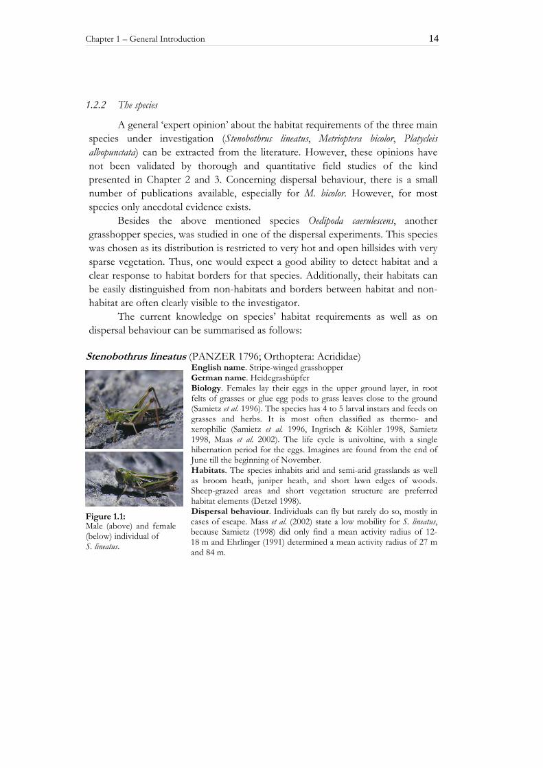
English name. Stripe-winged grasshopper German name. Heidegrashüpfer Biology. Females lay their eggs in the upper ground layer, in root felts of grasses or glue egg pods to grass leaves close to the ground (Samietz et al. 1996). The species has 4 to 5 larval instars and feeds on grasses and herbs. It is most often classified as thermo- and xerophilic (Samietz et al. 1996, Ingrisch & Köhler 1998, Samietz 1998, Maas et al. 2002). The life cycle is univoltine, with a single hibernation period for the eggs. Imagines are found from the end of June till the beginning of November. Habitats. The species inhabits arid and semi-arid grasslands as well as broom heath, juniper heath, and short lawn edges of woods. Sheep-grazed areas and short vegetation structure are preferred habitat elements (Detzel 1998). Dispersal behaviour. Individuals can fly but rarely do so, mostly in cases of escape. Mass et al. (2002) state a low mobility for S. lineatus, because Samietz (1998) did only find a mean activity radius of 12-18 m and Ehrlinger (1991) determined a mean activity radius of 27 m and 84 m.
Figure 1.1: Male (above) and female (below) individual of S. lineatus.
Chapter 1 – General Introduction 15
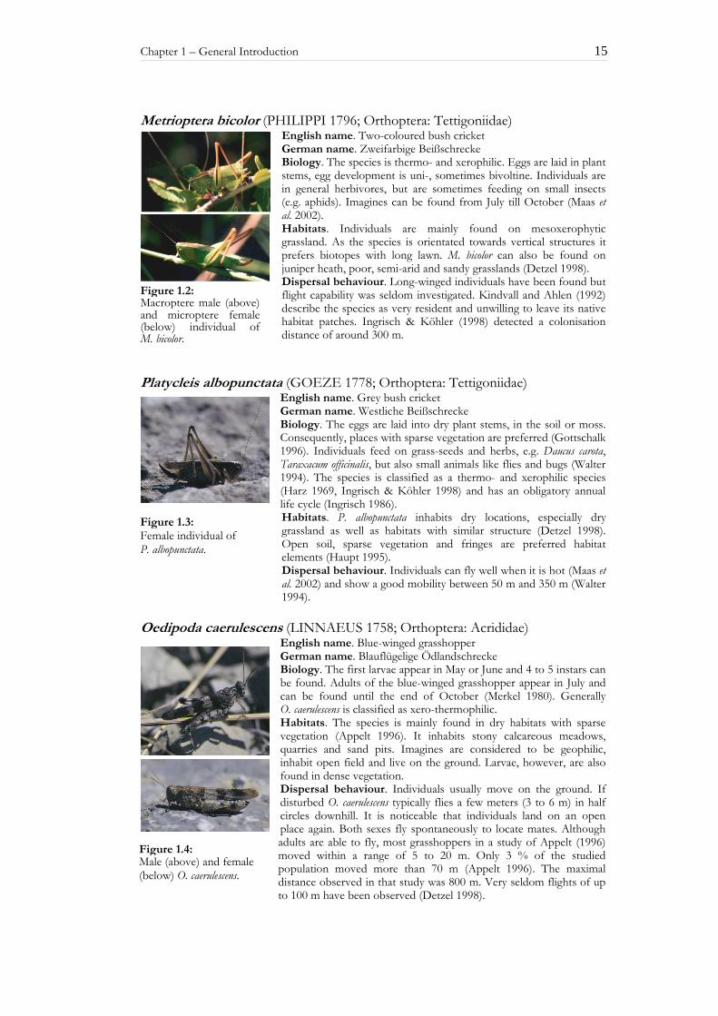
Metrioptera bicolor (PHILIPPI 1796; Orthoptera: Tettigoniidae) English name. Two-coloured bush cricket German name. Zweifarbige Beißschrecke Biology. The species is thermo- and xerophilic. Eggs are laid in plant stems, egg development is uni-, sometimes bivoltine. Individuals are in general herbivores, but are sometimes feeding on small insects (e.g. aphids). Imagines can be found from July till October (Maas et al. 2002). Habitats. Individuals are mainly found on mesoxerophytic grassland. As the species is orientated towards vertical structures it prefers biotopes with long lawn. M. bicolor can also be found on juniper heath, poor, semi-arid and sandy grasslands (Detzel 1998). Dispersal behaviour. Long-winged individuals have been found but flight capability was seldom investigated. Kindvall and Ahlen (1992) describe the species as very resident and unwilling to leave its native habitat patches. Ingrisch & Köhler (1998) detected a colonisation distance of around 300 m.
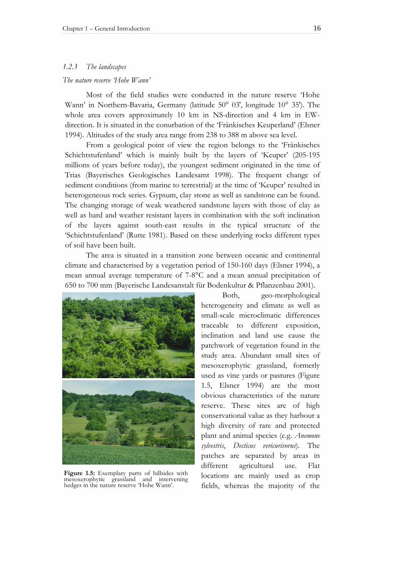
Platycleis albopunctata (GOEZE 1778; Orthoptera: Tettigoniidae) English name. Grey bush cricket German name. Westliche Beißschrecke Biology. The eggs are laid into dry plant stems, in the soil or moss. Consequently, places with sparse vegetation are preferred (Gottschalk 1996). Individuals feed on grass-seeds and herbs, e.g. Daucus carota, Taraxacum officinalis, but also small animals like flies and bugs (Walter 1994). The species is classified as a thermo- and xerophilic species (Harz 1969, Ingrisch & Köhler 1998) and has an obligatory annual life cycle (Ingrisch 1986). Habitats. P. albopunctata inhabits dry locations, especially dry grassland as well as habitats with similar structure (Detzel 1998). Open soil, sparse vegetation and fringes are preferred habitat elements (Haupt 1995). Dispersal behaviour. Individuals can fly well when it is hot (Maas et al. 2002) and show a good mobility between 50 m and 350 m (Walter 1994).
Oedipoda caerulescens (LINNAEUS 1758; Orthoptera: Acrididae)
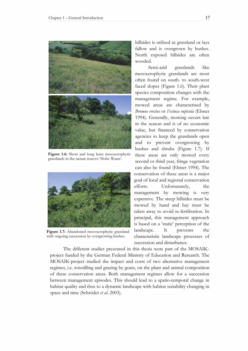
English name. Blue-winged grasshopper German name. Blauflügelige Ödlandschrecke Biology. The first larvae appear in May or June and 4 to 5 instars can be found. Adults of the blue-winged grasshopper appear in July and can be found until the end of October (Merkel 1980). Generally O. caerulescens is classified as xero-thermophilic. Habitats. The species is mainly found in dry habitats with sparse vegetation (Appelt 1996). It inhabits stony calcareous meadows, quarries and sand pits. Imagines are considered to be geophilic, inhabit open field and live on the ground. Larvae, however, are also found in dense vegetation. Dispersal behaviour. Individuals usually move on the ground. If disturbed O. caerulescens typically flies a few meters (3 to 6 m) in half circles downhill. It is noticeable that individuals land on an open place again. Both sexes fly spontaneously to locate mates. Although adults are able to fly, most grasshoppers in a study of Appelt (1996) moved within a range of 5 to 20 m. Only 3 % of the studied population moved more than 70 m (Appelt 1996). The maximal distance observed in that study was 800 m. Very seldom flights of up to 100 m have been observed (Detzel 1998).
Figure 1.4: Male (above) and female (below) O. caerulescens.
Figure 1.3: Female individual of P. albopunctata.
Figure 1.2: Macroptere male (above) and microptere female (below) individual of M. bicolor.
Chapter 1 – General Introduction 16
1.2.3 The landscapes
The nature reserve ‘Hohe Wann’
Most of the field studies were conducted in the nature reserve ‘Hohe Wann’ in Northern-Bavaria, Germany (latitude 50° 03′, longitude 10° 35′). The whole area covers approximately 10 km in NS-direction and 4 km in EW-direction. It is situated in the conurbation of the ‘Fränkisches Keuperland’ (Elsner 1994). Altitudes of the study area range from 238 to 388 m above sea level.
From a geological point of view the region belongs to the ‘Fränkisches Schichtstufenland’ which is mainly built by the layers of ‘Keuper’ (205-195 millions of years before today), the youngest sediment originated in the time of Trias (Bayerisches Geologisches Landesamt 1998). The frequent change of sediment conditions (from marine to terrestrial) at the time of ‘Keuper’ resulted in heterogeneous rock series. Gypsum, clay stone as well as sandstone can be found. The changing storage of weak weathered sandstone layers with those of clay as well as hard and weather resistant layers in combination with the soft inclination of the layers against south-east results in the typical structure of the ‘Schichtstufenland’ (Rutte 1981). Based on these underlying rocks different types of soil have been built.
The area is situated in a transition zone between oceanic and continental climate and characterised by a vegetation period of 150-160 days (Elsner 1994), a mean annual average temperature of 7-8°C and a mean annual precipitation of 650 to 700 mm (Bayerische Landesanstalt für Bodenkultur & Pflanzenbau 2001).
Both, geo-morphological heterogeneity and climate as well as small-scale microclimatic differences traceable to different exposition, inclination and land use cause the patchwork of vegetation found in the study area. Abundant small sites of mesoxerophytic grassland, formerly used as vine yards or pastures (Figure 1.5, Elsner 1994) are the most obvious characteristics of the nature reserve. These sites are of high conservational value as they harbour a high diversity of rare and protected plant and animal species (e.g. Anemone sylvestris, Decticus vericurivorus). The patches are separated by areas in different agricultural use. Flat locations are mainly used as crop fields, whereas the majority of the
Figure 1.5: Exemplary parts of hillsides with mesoxerophytic grassland and intervening hedges in the nature reserve ‘Hohe Wann’.
Chapter 1 – General Introduction 17
hillsides is utilised as grassland or lays fallow and is overgrown by bushes. North exposed hillsides are often wooded.
Semi-arid grasslands like mesoxerophytic grasslands are most often found on south- to south-west faced slopes (Figure 1.6). Their plant species composition changes with the management regime. For example, mowed areas are characterised by Bromus erectus or Festuca rupicola (Elsner 1994). Generally, mowing occurs late in the season and is of no economic value, but financed by conservation agencies to keep the grasslands open and to prevent overgrowing by bushes and shrubs (Figure 1.7). If these areas are only mowed every second or third year, fringe vegetation can also be found (Elsner 1994). The conservation of these areas is a major goal of local and regional conservation efforts. Unfortunately, the management by mowing is very expensive. The steep hillsides must be mowed by hand and hay must be taken away to avoid re-fertilisation. In principal, this management approach is based on a ‘static’ perception of the landscape. It prevents the characteristic landscape processes of succession and disturbance.
The different studies presented in this thesis were part of the MOSAIK-project funded by the German Federal Ministry of Education and Research. The MOSAIK-project studied the impact and costs of two alternative management regimes, i.e. rototilling and grazing by goats, on the plant and animal composition of these conservation areas. Both management regimes allow for a succession between management episodes. This should lead to a spatio-temporal change in habitat quality and thus to a dynamic landscape with habitat suitability changing in space and time (Schröder et al. 2003).
Figure 1.6: Short and long lawn mesoxerophytic grasslands in the nature reserve ‘Hohe Wann’.
Figure 1.7: Abandoned mesoxerophytic grassland with ongoing succession by overgrowing bushes.
Chapter 1 – General Introduction 18
The nature reserve ‘Leutratal’
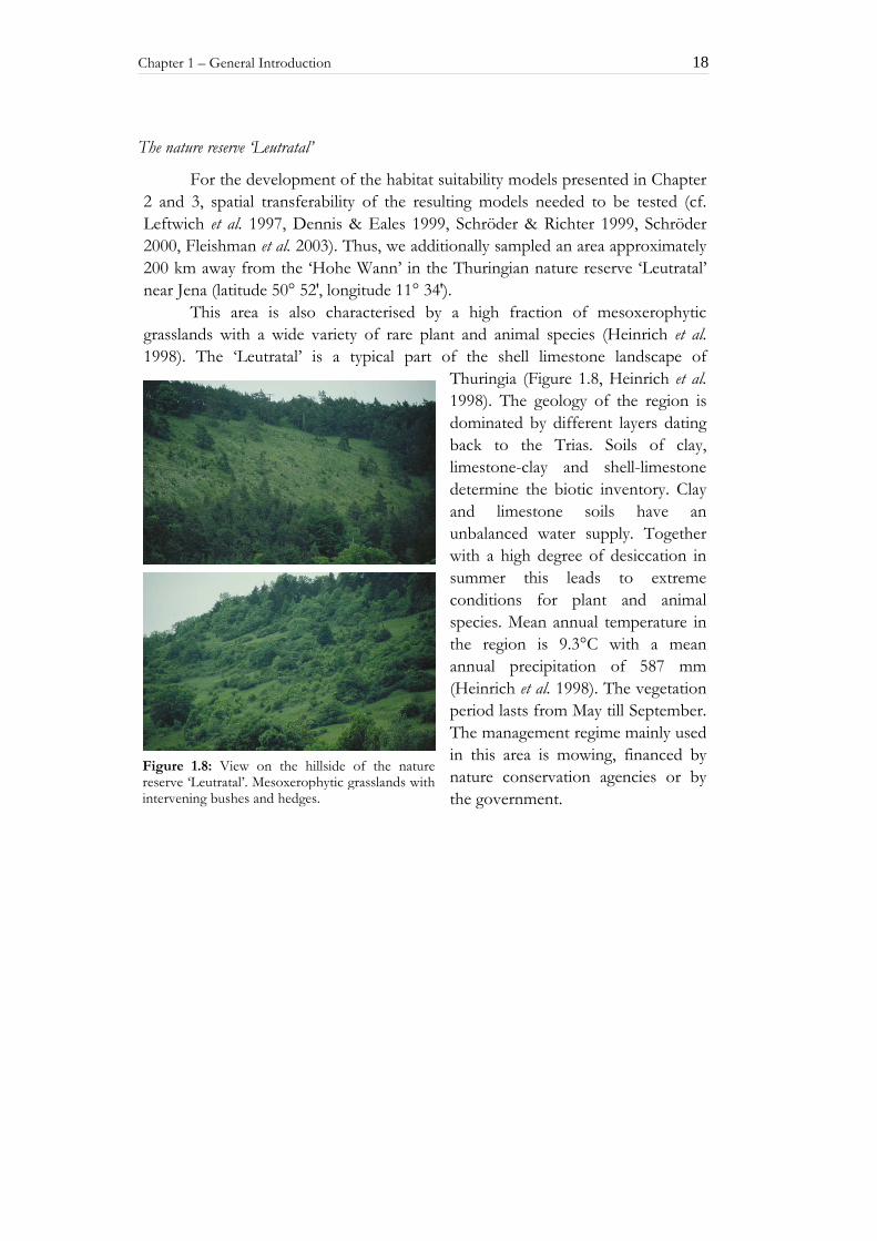
For the development of the habitat suitability models presented in Chapter 2 and 3, spatial transferability of the resulting models needed to be tested (cf. Leftwich et al. 1997, Dennis & Eales 1999, Schröder & Richter 1999, Schröder 2000, Fleishman et al. 2003). Thus, we additionally sampled an area approximately 200 km away from the ‘Hohe Wann’ in the Thuringian nature reserve ‘Leutratal’ near Jena (latitude 50° 52′, longitude 11° 34′).
This area is also characterised by a high fraction of mesoxerophytic grasslands with a wide variety of rare plant and animal species (Heinrich et al. 1998). The ‘Leutratal’ is a typical part of the shell limestone landscape of
Thuringia (Figure 1.8, Heinrich et al. 1998). The geology of the region is dominated by different layers dating back to the Trias. Soils of clay, limestone-clay and shell-limestone determine the biotic inventory. Clay and limestone soils have an unbalanced water supply. Together with a high degree of desiccation in summer this leads to extreme conditions for plant and animal species. Mean annual temperature in the region is 9.3°C with a mean annual precipitation of 587 mm (Heinrich et al. 1998). The vegetation period lasts from May till September. The management regime mainly used in this area is mowing, financed by nature conservation agencies or by the government.
Figure 1.8: View on the hillside of the nature reserve ‘Leutratal’. Mesoxerophytic grasslands with intervening bushes and hedges.
Chapter 1 – General Introduction 19
1.3 CONCEPTUAL FRAMEWORK
Spatial heterogeneity of the environment as well as fragmentation of habitats generally result in a mosaic-like or patchy distribution of organisms (Settele 1998). The spatial constellation of habitats with high habitat capacity (in the following: suitable habitats/patches) determines the spatial distribution of populations. Individuals inhabit suitable habitats and use the area in between at best for the exchange between patches (Settele 1998). For the description of such spatially structured populations, different classifications of populations have been introduced based on spatial structure of populations and the exchange of individuals (see Box 1).
Spatially structured populations can only survive in regional connected assemblages as survival probability of small and/or isolated populations may be low (Veith & Klein 1996). Therefore, they cannot be described with classical population models for single populations and cannot account for the mutual influence on populations in a landscape (Andrewartha & Birch 1954, Poethke et al. 1996a). A closer examination of spatially structured populations at a landscape scale became first possible with the development of models of island biogeography (McArthur & Wilson 1967) and metapopulation theory (Levins 1970, Hanski & Gilpin 1997). In recent years the metapopulation concept (Levins 1969, 1970) has become increasingly popular in theoretical as well as empirical studies on the spatial and temporal structure of populations (e.g. Hanski 1994a, b, Hill et al. 1996, Poethke et al. 1996a, b, Reich & Grimm 1996, Settele 1998).
A metapopulation is a regional assemblage of locally connected populations inhabiting discrete habitat patches, and can be described as a population of populations (Levins 1970, Halle 1996). Local patches have a substantial risk of extinction, but can also be (re-) colonised; metapopulations are thus characterised by (substantial) population turnover (Levins 1970, Hanski & Gilpin 1991). Fundamentally, such a population assemblage can only persist if the extinction probability of local populations is lower than their colonisation probability. Additionally, to prevent a random concurrent extinction of all local populations, a sufficient number of local patches must belong to the metapopulation (Poethke et al. 1996a, b). It is obvious that the probability that a certain patch will be occupied at any moment in time depends on its capacity as well as its isolation.
To predict occupancy patterns of patches in metapopulations (Ij) Hanski (1994a) presented a simple stochastic model that corresponds to the island-model of MacArthur & Wilson (1967) for the prediction of species number on islands differing in size and isolation. However, Hanski (1994a) assumes that extinction risk (Ej) as well as colonisation probability (Cj) are patch specific:

Chapter 1 – General Introduction 20
jj
jj CE
CI
+= (1.1)
Additionally, the rescue-effect (Brown & Kodrik-Brown 1977), the reduction of extinction probability due to immigration can be included in the model. Empirically, extinction probabilities may either be estimated from long-term observation data (see Hanski & Zhang 1993, Hanski et al. 1994, Hill et al. 1996) or by using values extracted from simulations which are based on measures that are more readily determined (Poethke et al. 1996b).
Box 1: Models of spatial structure and interactions of populations
A population may be defined as a group of interacting individuals of a species (breeding and competing with each other) occupying a particular space at a particular time, at least partially isolated from other populations of the same species (Dempster & McLean 1998, Krebs 2001). However, what actually constitutes a population will vary from species to species and from study to study depending on spatial scale and focus of the study (Begon et al. 1990). For the description of a single population one may quantify different population properties (e.g. population size). Alternatively, population structure, e.g. demographic/genetic structure, spatial structure, sex ratio or the distribution of individuals in time, may be used for characterisation. Although in reality transitions between different classes are fluent, one may differentiate the following types of populations based on spatial structure and exchange of individuals between habitat patches:
Continuous population Each single population is sufficiently large and able to survive over large time periods (of course the extinction probability of any population reaches a value of 1 if time goes to infinity; Veith & Klein 1996)
Patchy population Isolation between populations has reached a high degree but frequent exchange of individuals takes place. In this case a quasi continuous population is reached (Harrison 1991). Metapopulation A regionally connected population of local populations (Levins 1970) on qualitatively similar patches, with an own, independent population dynamic and a high local extinction probability. Populations are in an equilibrium between extinction and colonisation (island-equilibrium model ). If some populations have a high and others a low probability of survival and if locally extinct patches are colonised by individuals from quasi-persistent populations the core satellite model/mainland-island model can be applied (Boorman & Levitt 1973). In this model patches vary in patch size only. If especially the peripheral patches are qualitatively worse than a central patch one would call the system a source-sink model (Pulliam 1988). In that situation recolonisation becomes a ‘one-way street’ from the central source-population to peripheral sinks. Sink-populations cannot survive without constant immigration.

Chapter 1 – General Introduction 21
The two main aspects leading to extinction are low patch area and/or low patch quality, which both contribute to patch capacity. The area of a patch can be easily obtained from a cartographic map or geographic information system (GIS) whereas the quality depends on different environmental conditions. Based on the distribution of a species across different environmental parameters conclusions about patch quality and thus patch capacity are possible (see paragraph 1.3.1 this Chapter).
The probability that a patch will be colonised is mainly determined by its reachability, i.e. the probability that a dispersing individual will reach the patch, as well as the probability that immigrants can establish a population in the new patch. The reachability of a patch depends on the number and capacity of occupied patches in its surrounding. To determine the reachability of patches a large number of studies have been conducted in recent years. Especially the dispersal process has been intensively investigated with studies ranging from empirical mark- and recapture studies (e.g. Baguette & Nève 1994, Hill et al. 1996, Brommer & Fred 1999, Kindvall 1999, Roland et al. 2000, Ricketts 2001) to theoretical investigations on evolutionary aspects of the dispersal process (Hovestadt et al. 2000, Hovestadt et al. 2001, Poethke & Hovestadt 2002, Poethke et al. 2003; see paragraph 1.3.2 this Chapter).
1.3.1 Habitat suitability and patch capacity
Habitat suitability together with patch area determines patch capacity. To measure habitat suitability the needs of a species must be known. Morrison et al. (1998) define a species’ habitat as an area with the combination of resources and environmental conditions that allows individuals to survive and to reproduce. From an evolutionary point of view, high habitat quality means high fitness of individuals in that specific habitat. Thus, different kinds of habitat result in different levels of fitness or suitability in the landscape (in evolutionary time suitability is equivalent to fitness, Krebs 2001). Habitat suitability is not constant but affected by many factors within the habitat, such as food supply, shelter and predators (Krebs 2001). The resulting occurrence of a species describes its realised niche (see Box 2). Vice versa one can infer a species’ habitat requirements from its distribution across environmental variables (Huston 1994, Rosenzweig 1995). The concept of the niche and thus the premise that predictable relations exist between the occurrence of a species and certain features of its environment is the underlying principle in habitat suitability modelling (Rosenzweig 1981).
The analyses of species-habitat or species-environment relationships has a long history and was first institutionalised with the development of habitat suitability index-models (HSI-models) by the U.S. Fish & Wildlife Service (1981). Species-environment models may either address single species or more complex multi-species assemblages when identifying relations between occurrence and environmental features at a variety of scales (local to biogeographic; Verner et al. 1986, Kuhn 1998, Bonn & Schröder 2001, Heglund 2002, Storch 2002).
Chapter 1 – General Introduction 22
Examples of models include prediction of species occurrence, distribution and abundance using habitat suitability, pattern recognition, and wildlife-habitat relation models (Morrison et al. 1998).
Box 2: The concept of the niche – History and Application
Historically, Grinnell (1917) first emphasized the environmental requirements of a species and considered the niche a fundamental distributional unit of a species. Elton (1930) later defined the niche as the ‘role’ of the species in the community, which is a behaviour-based concept. This definition highlighted the role other species play in shaping the expressed niche of an organism. Both definitions are considered conceptually vague and years later a quantitative concept of the niche was proposed by Hutchinson (1957). Based on this concept, the niche is best described by the coordinates of a species with n-dimensional resource axes and combines both the behavioural and the distributional concepts of Elton and Grinnell (Cao 1995, Morrison et al. 1998). Thus, generally data on a multitude of variables within the environment are collected, and the measures most strongly related to the occurrence of the species are selected. With this measures one can devise models that generally describe the location of that species in just a few dimensions (Krebs 2001). In reality, the presence of competing species restricts a given species to a narrower range of conditions – its ‘realized’ niche. The foundation of our current modelling efforts lies in the characterization of a species’ realized niche rather than simply determining habitat relations. Theoretically, along an environmental gradient most species should exhibit maximum density at some point (Gauch & Chase 1974).
In the beginning these models were mostly based on ‘expert knowledge’ and general statements on habitat preferences of specific species. With the increasing availability of statistical software, an overwhelming array of statistical methods was employed in the assessment of species’ relations to their environment. The distribution, or response of an organism in regard to a given environmental variable is generally considered nonlinear (Gauch & Chase 1974, Austin 1976, Heglund et al. 1994). Multivariate statistics were established for the quantitative analyses of empirical data and for model development (Brennan et al. 1986, Morrison et al. 1998). Statistical procedures that were often used are discriminant analyses as well as general linear models (GLM, Guisan & Zimmermann 2000).
For a variety of reasons logistic regression analysis has gained importance as a non-parametric, non-linear alternative to discriminant analysis to model species-habitat relationships (Guisan & Zimmermann 2000, Guisan et al. 2002). First, this procedure is the only suitable one that allows an analyses of categorial variables (Capen et al. 1986, Kleyer et al. 1999/2000). Second, this method is favoured because better results in classification of results and more robust models are received. Additionally, coefficients are easy to interpret and a variety of measures for model calibration and discrimination have been developed

Chapter 1 – General Introduction 23
(Nagelkerke 1991, Buckland et al. 1997, Fielding & Bell 1997, Backhaus 2000, Hosmer & Lemeshow 2000, Manel et al. 2001, Austin 2002). Logistic regression examines the relationship between independent variables (habitat parameters) and a dichotomous dependent variable (incidence of a specific species, Trexler & Travis 1993). This relationship can be expressed by the following equation:
)...( 11011
)1(kk xxe
yP βββ +++−+== (1.2)
P(y = 1) : probability that the dependent variable (i.e. incidence) takes the value 1 (i.e. species present) β0 : constant
xk : independent predictor variables βk : coefficient of independent variable
The approach described above provides a fairly static picture of populations, while in reality species-environment relations are dynamic. Populations fluctuate in abundance between years in response to a number of factors, including weather, food, conditions, habitat, predator abundance, and parasite loads (Wiens 1989 ). As habitats may vary in time and space, models should be evaluated in both. Ideally, models should be developed and tested using independent data sets derived from field studies in different years and regions (Fleishman et al. 2003). As this is time consuming and cannot be done in every study different methods of re-sampling evaluation have been suggested (for a review see Verbyla & Litvatitis 1989). For example, bootstrap techniques have shown good results. Through re-sampling (with replacement), the bootstrap allows to estimate the optimism (bias) in measures of predictive accuracy and, then, subtract the estimate of optimism from the initial apparent measure to obtain a bias-corrected estimate (Efron & Tibshirani 1993).
In this thesis robust habitat suitability models are developed and evaluated for different grasshopper and bush cricket species with the use of single and multiple parameter logistic regression analyses (Chapter 2). Additionally, these models together with models for two butterfly species are tested for their transferability within one insect group and between the two groups (Chapter 3). The resulting quantitative predictions of species occurrences in a specific landscape under different management scenarios may be used as the basis for the prediction of long term survival of populations in population viability analyses (Schröder et al. 2003).
1.3.2 Dispersal
Dispersal (see Box 3) is one of the most important, yet least understood, processes in ecology, population biology, and evolution, as it gives populations, communities, and ecosystems their characteristic texture in space and time (Kenward et al. 2001, Macdonald & Johnson 2001). It acts as the ‘glue’ that binds populations together (Wiens 2001) and has diverse ramifications for population
Chapter 1 – General Introduction 24
dynamics (e.g. avoidance of kin competition, speciation by founder effects). The most fundamental population dynamic consequences at the level of local populations and metapopulations are population regulation via density-dependent emigration and large-scale persistence of classical metapopulations due to establishment of new populations and rescue of threatened populations (e.g. Brown & Kodrik-Brown 1977, Hanski 2001).
Box 3: Definitions of dispersal
Movement reveals different forms (Dingle 1996). Dispersal is often distinguished from migration by the fact that the dispersal process is a ‘one way street’ with no return of the individual (in contrast to migration, e.g. birds migrating to Africa in winter and back in summer, Begon et al. 1990). Howard (1960) defined dispersal as ‘the permanent movement by an individual from birth place to place of reproduction’ (Kenward et al. 2001). This corresponds to Bullock et al. (2001) who use a common definition of dispersal as ‘intergenerational movement’. They thus exclude so-called ‘dispersal in time’ (e.g. seed banks) as well as foraging movements of animals. Especially in the case of birds this became complicated as individuals were repeatedly recaptured at breeding sites. Thus a common separation introduced by Greenwood (1980) and also used by others (Greenwood & Harvey 1982) separates natal and breeding dispersal. This definition is also used by Clobert et al. (2001): The term natal dispersal, is the movement between the natal area or social group and the area or social group where breeding first takes place, and breeding dispersal, is the movement between two successive breeding areas or social groups. In practice, e.g. if movements are recorded in detail by radio tracking an animal along its ‘life path’ (Baker 1978, Bullock et al. 2001), problems arise, resulting in a further detailed terminology (see Kenward et al. 2001). Thus, generally the above mentioned definitions are used and specified in more detail depending on study species and focus of the research (see Bullock et al. 2001, Clobert et al. 2001).
Biologists from the two main fields concerned with dispersal, behavioural and population ecology, have typically taken two almost entirely different approaches to study dispersal, both with regard to questions asked and the methods used (Andreassen et al. 2001). Behavioural ecologists have typically been concerned with understanding the proximate and ultimate causes of dispersal (e.g. Bengtsson 1978) and based their conclusions mainly on empirical studies. Population biologists on the other hand have typically considered dispersal as a key process for understanding population dynamics, spatial synchrony, population genetics (e.g. Stenseth 1983) and the evolution of dispersal (Hovestadt et al. 2000, Hovestadt et al. 2001, Poethke & Hovestadt 2002, Poethke et al. 2003). They have examined their problems often by using theoretical modelling studies (including metapopulation dynamics; Hanski & Gilpin 1997). Although, the studies on dispersal in this thesis focus on the behavioural aspects of dispersal, spatially explicit individual based modelling is used as a tool to derive adequate hypothesis (Chapter 5) or to extrapolate individual behaviour to a landscape level (Chapter 6). Nevertheless, the results from Chapter 4-6 will also contribute to a better

Chapter 1 – General Introduction 25
understanding of population dynamic consequences of dispersal, as they adjust frequently made assumptions in population models which are not supported by empirical studies of dispersal behaviour.
Generally dispersal can be divided into three phases: emigration, transfer and immigration (see Andreassen et al. 2001). Most studies on dispersal have, implicitly or explicitly, adopt the view that individuals leave a given patch or population, cross a gap, and (somehow) end up later in another patch or population (Wiens 2001). Both decisions, when to leave and when to stop, vary among species and individuals. Whether an individual leaves a patch, for example, may depend on the mode of dispersal, genetic predisposition to disperse, local population density, habitat change, age, or reproductive status, among other factors (Wiens 2001). The decision to stop may involve various elements of habitat selection or patch choice, such as conspecific attraction, habitat quality, or physiological factors.
The simplest and arguably most efficient way to disperse is to follow a straight path from the origin to the stopping place. This view of dispersal is fostered by mark-recapture studies, in which the linear distance between the marking location and the recapture location provides empirical measure of dispersal distance (Wiens 2001). Thus, island biogeography (MacArthur & Wilson 1967) or metapopulation and source-sink models of population dynamics (Pulliam 1988, Hanski & Gilpin 1997) consider the linear distance of an island or subpopulation from a source to be a key determinant of colonisation probabilities. Generally, the dispersal process of individuals is described in terms of a dispersal-distance function (Wiens 2001). A common used form of such a function has been proposed by Hanski (1994a, b):
decdP α−= *)( (1.3)
It describes the probability to settle at a specific place (P(d)) as a function of the Euclidian distance (d) between two individual patches and a species specific dispersal parameter (α). The influence of spatial arrangement of patches in a landscape on the exchange of individual between patches is often neglected (but see Chapter 6). Additionally, in such models the matrix is featureless and ‘distance’ is measured as a linear value, a ‘gap’ to be crossed. Indeed, both empirical studies (Grubb & Doherty 1999) and models (With & King 1999a, b) of gap-crossing focus on size of the gaps but not on their composition. All of these approaches thus assume that individuals either move from one place to another in a straight line or in a random walk unaffected by any environmental features.
The area between the start- and the end-point of dispersal, however, usually is a richly textured mosaic of patches of different shape, sizes, arrangements, and qualities. It thus becomes important to know, how individuals move within different habitats (Wiens 2001, see Chapter 4). Information about
Chapter 1 – General Introduction 26
such movement rules may then be used to model long distance dispersal in real landscapes (Kindvall 1999).
Independent of the degree of heterogeneity that exists in a landscape individuals should benefit if they are able to detect suitable habitat from distance. This should especially be the case for a habitat specialist. The analyses of such detection distances or perceptual ranges is often conducted with direct observations of individuals’ movement behaviour. In Chapter 5 I present an approach to test for the detection ability of species even though direct observations are not possible. Individual based simulations are used to develop adequate null hypothesis with different theoretical assumptions about the underlying movement rules. Simulation results are then compared exemplarily with field data from arrival rates of a grasshopper species.

Chapter 2
Habitat suitability models for the conservation of thermophilic grasshoppers
and bush crickets
with Julia Voss, Boris Schröder and Hans-Joachim Poethke.
SUBMITTED TO BIOLOGICAL CONSERVATION
Abstract. In our study we investigate habitat preferences of the two bush cricket species Metrioptera bicolor and Platycleis albopunctata and the grasshopper species Stenobothrus lineatus in the nature reserve ‘Hohe Wann’ (Northern Bavaria, Germany). To determine species habitat preferences, we developed statistically derived habitat suitability models. For validation of the models in time and space, the study was repeated in a second year and in a second study area. We found that vegetation structure as well as topographical parameters like the exposition determine habitat selection. Besides these factors which are rather costly to determine at the landscape level, the type of biotope seems to be the most reliable factor that determines the occurrence of the studied species. Internal validation demonstrates that habitat suitability models based on this factor allowed to set up robust models. Inclusion of the surrounding landscape into the analysis resulted only in the case of S. lineatus in a significant influence of the plot surrounding in a radius between 25 m and 50 m. None of the species showed distinct microhabitat preferences. With the help of this model analyses of habitat suitability can easily be carried out on the basis of already existing vegetation maps for the conservation of the three species under study. Thus, our results can serve as a basis for the estimation of the survival probability of the species studied.

Chapter 2 – Habitat suitability for grasshoppers and bush crickets 29
2.1 INTRODUCTION
The conservation of the fauna and flora of mesoxerophytic grasslands is a major topic in (Central European) conservation biology as these areas are inhabited by a variety of rare and protected thermophilic plant and animal species (Poschlod & Schumacher 1998). Mesoxerophytic grasslands are found on poor soil conditions. These areas are often inaccessible at strong inclination and provide only low nutritioned food. As a consequence of the low economic value utilization of these areas decreases and more and more areas are abandoned. The grasslands are thus exposed to successional processes which results in the loss of valuable species. Thus, the management of such areas has increasingly been occupied with the conservation of specific successional stages and the prevention of further succession. To predict which successional stages are suitable for specific species reliable information on species specific habitat requirements is needed. Such information is a critical prerequisite for the choice of protected areas, the design of management strategies, and the assessment of possible effects of various land-use changes (Fielding & Haworth 1995, Oppel et al. in press) on the survival of plant and animal species.
In recent years statistically derived habitat suitability models have become a common tool for the estimation of critical factors that determine habitat suitability for and habitat selection by a species (Ferrier 1991, Lindenmayer et al. 1991, Pearce et al. 1994, Guisan & Zimmermann 2000, Pearce & Ferrier 2000a, b). Such models use the presence and absence of a species at a set of survey sites in relation to environmental or habitat variables to detect functional relationships between a species and its environment (Guisan & Zimmermann 2000, Austin 2002). Besides other methods logistic regression is a well established method to perform such habitat modelling (Trexler & Travis 1993, Guisan & Zimmermann 2000), because it is a simple and robust procedure, and yields comparatively high performance as well as biologically interpretable model parameters (Manel et al. 1999a).
One problem with models based on simple presence/absence data is that data are only snap-shots from a certain time period and a certain region. Such models are static (Guisan & Zimmermann 2000) and need to be validated in space and time before they can be extrapolated to other areas (Morrison et al. 1998). To obtain an unbiased estimate of a model’s predictive performance, evaluation is best undertaken with independent data collected from sites others than those used to develop the model (Schröder & Richter 1999, Pearce & Ferrier 2000a, b). Alternatively, internal validation techniques can be applied (Lehmann et al. 2002, Reineking & Schröder 2003). As habitat selection behaviour is scale-dependent different spatial scales should be taken into account when studying species specific habitat preferences (Orians & Wittenberger 1991).

Chapter 2 – Habitat suitability for grasshoppers and bush crickets 30
In this study we investigate habitat selection of two bush crickets and one grasshopper species typically found on mesoxerophytic grassland. We ask for biotic and abiotic site parameters relevant for the habitat preferences of the three species and how species occurrence can be predicted with simple and easily available measures. To test for scale effects, we looked for preferred microhabitats within experimental plots and then analysed the influence of the surrounding types of biotope on the occurrence probability of the species. In our analyses we present a straightforward way to determine habitat suitability using logistic regression analyses and to evaluate and validate such models. Thereby we combine different methods independently suggested by other authors (Fielding & Bell 1997, Guisan & Zimmermann 2000, Schröder 2000).
2.2 MATERIAL AND METHODS
2.2.1 The species
From the literature and experts a general ‘expert opinion’ about the habitat requirements of the three species can be extracted. However, these opinions have not yet been confirmed by thorough field studies of the kind presented in this article. Current knowledge on species habitat requirements can be summarized as follows:
Stenobothrus lineatus
The stripe-winged grasshopper Stenobothrus lineatus (PANZER 1796; Orthoptera: Acrididae) is a medium-sized to large grasshopper species (body length: 15 – 26 mm). It is thermo- and xerophilic and inhabits arid and semi-arid grasslands as well as broom heath, juniper heath, and short lawn edges of woods. Sheep-grazed areas and short vegetation structure are preferred habitat elements (Detzel 1998).
Metrioptera bicolor
The two-coloured bush cricket Metrioptera bicolor (PHILIPPI 1796; Orthoptera: Tettigoniidae) is medium-sized (body length: 15 – 18 mm), thermo- and xerophilic, and mainly inhabits mesoxerophytic grassland As it is orientated towards vertical structures the species prefers long lawn biotopes. Metrioptera bicolor can also be found on juniper heath, poor grassland, semiarid and sandy grasslands (Detzel 1998). Kindvall and Ahlen (1992) describe the species as very resident and unwilling to leave its native habitat patches.

Chapter 2 – Habitat suitability for grasshoppers and bush crickets 31
Platycleis albopunctata
The grey bush cricket Platycleis albopunctata (GOEZE 1778; Orthoptera: Tettigoniidae) is a medium- to large-sized bush cricket species (body length: 18 – 22 mm). It is classified as a thermo- and xerophilic species (Harz 1969, Ingrisch & Köhler 1998), which inhabits dry locations, especially dry grassland as well as habitats with similar structure (Detzel 1998). Open soil, sparse vegetation and fringes are preferred habitat elements. In the nature reserve ‘Hohe Wann’ it is therefore found within a more narrow distribution than M. bicolor.
2.2.2 Field work
The study was conducted in August and September in the years 2001 and 2002 in the nature reserve ‘Hohe Wann’ in Northern-Bavaria, Germany (latitude 50° 03′, longitude 10° 35′). The study area is characterised by a patchwork of vegetation caused by the geological and geomorphological heterogeneity of the area and small-scale microclimatic differences traceable to different exposition, inclination and land use. Additionally, agricultural fields are usually very small. The most obvious characteristic of the nature reserve are abundant sites of mesoxerophytic grassland, formerly used as vine yards (Elsner 1994). These patches are separated by agricultural landscape of different use. The whole area covers approximately 10 km in NS-direction and 4 km in EW-direction.
Incidence of the grasshopper and bush cricket species was recorded on 146 experimental sites selected by stratified random sampling across the ten main types of biotope occurring in the region. To increase the resolution of our approach we sampled with high effort in habitats with – based on prior knowledge – uncertain status regarding the species’ occurrence (Table 2.1).
We used a Geographic information system (GIS, ESRI ArcView 3.2) to determine the main types of biotope in the area and sampled each type (Table 2.1). Distance between two experimental sites was at least 30 m. We characterised each site by the vegetation structure of a randomly chosen 1 m2 plot. For the analysis of micro structural preference of the grasshoppers and bush crickets vegetation structure was also recorded at 1 m2 plots immediately surrounding the point where individuals of the species under study were found. Vegetation structure analysis included estimates of horizontal plant cover, vertical plant cover and vegetation height (cf. Sundermeier 1999). Additionally we recorded the type of biotope, the actual management regime, the inclination and exposition of the plots.
For the determination of grasshopper and bush cricket incidence we carried out transect sampling (inter-transect distance = 1.5m) on the experimental sites (15 m x 15 m). The census was terminated (i) as soon as a specimen was found or (ii) after a maximum of 20 minutes of sampling time. As the activity of grasshoppers and bush crickets strongly depends on weather conditions, censuses were only carried out during ‘good’ weather condition (sunshine, cloud cover

Chapter 2 – Habitat suitability for grasshoppers and bush crickets 32
< 3/8; air temperature > 17 °C; wind speed < 4 m/s; Mühlenberg 1993) to ensure the same detection probability on all plots.
Table 2.1: Overview of sample plots, their distribution across types of biotope and frequency of occupancy for the three species under study. Results are shown for two years at sample site ‘Hohe Wann’ and one year at the sample site ‘Leutratal’.
P. albopunctata M. bicolor S. lineatus year location type of biotope
# of plots
occup. unocc. occup. unocc. occup. unocc.
2001 Hohe Wann
all 146 23 123 60 86 64 82
Extensively managed meadow
45 6 39 24 21 25 20
Intensively managed meadow
7 1 6 1 6 2 5
Inten. managed meadow meagre
24 - 24 5 19 7 17
mesoxerophytic grassland
26 9 17 18 8 21 5
fringe vegetation 10 7 3 9 1 9 1
crop field 8 - 8 1 7 - 8
fallow land 6 - 6 1 5 - 6
hedge 7 - 7 1 6 - 7
forest 7 - 7 - 7 - 7
thermophilic forest 6 - 6 - 6 - 6
2002 Hohe Wann
all 143 28 115 70 73 50 93
extensively managed meadow
45 13 32 25 20 16 29
Intensively managed meadow
8 1 7 4 4 1 7
Inten. managed meadow meagre
22 - 22 7 15 3 19
mesoxerophytic grassland
26 7 19 22 4 20 6
fringe vegetation 10 7 3 8 2 9 1
crop field 8 - 8 1 7 - 8
fallow land 6 - 6 2 4 1 5
hedge 7 - 7 1 6 - 7
forest 6 - 6 - 6 - 6
thermophilic forest 5 - 5 - 5 - 5
2002 Leutratal all 28 18 10 - - 16 12
extensively managed meadow
5 2 3 - - 4 1
Intensively managed meadow
5 - 5 - - 2 3
Inten. managed meadow meagre
5 2 3 - - 1 4
mesoxerophytic grassland
6 4 2 - - 6 0
fringe vegetation 3 2 1 - - 3 0
crop field 2 - 2 - - - 2
hedge 3 1 2 - - 1 2
Chapter 2 – Habitat suitability for grasshoppers and bush crickets 33
To test for the transferability of the resulting habitat suitability models in space (cf. Leftwich et al. 1997, Dennis & Eales 1999, Schröder & Richter 1999, Schröder 2000, Fleishman et al. 2003), we additionally sampled an area approximately 200 km away from our original study site in the Thuringian nature reserve Leutratal near Jena (latitude 50° 52′, longitude 11° 34′). This area is also characterised by a high fraction of mesoxerophytic grasslands with a wide variety of rare plant and animal species (Heinrich et al. 1998). Here we studied 28 experimental sites across 5 types of biotope (Table 2.1) in the same manner as in our main study area. Only two of our species (P. albopunctata, S. lineatus) could be found there, thus the spatial validation of the habitat suitability model for M. bicolor was not possible.
2.2.3 Statistical analyses
Development of habitat suitability models
We used single and multiple parameter logistic regression models to predict occurrence probability depending on plot parameters (Manel et al. 1999a, b, Hosmer & Lemeshow 2000). For the selection of adequate models we started with an univariate analysis to assess individual model variables independently from each other and to obtain information on each variable’s role (Hosmer & Lemeshow 2000). To choose uncorrelated parameters for the development of multiple parameter models we calculated all pairwise Spearman rank correlations and selected only one variable of those pairs showing correlation (ρs ≥ 0.7 (Fielding & Haworth 1995)). We did not use independent factors from a principal component analyses (PCA) because these turned out to create difficulties in their biological interpretation and are consequently difficult to use in conservation biology. As integrating measures for horizontal and vertical vegetation cover, we used the ‘total horizontal cover’, which describes the vertical structures at a plot (Sundermeier 1999), and the ‘percentage open ground’.
Initial single parameter models included all types of biotope investigated. Due to total separation causing numerical instabilities in some types of habitat we restricted our analyses to those types of biotope with at least minimal variation in occupancy. This was done to get a more detailed explanation of the species’ habitat requirements. Eliminated biotopes were included into our models by formulating rules, like ‘If forest then not suitable habitat’. These can be easily implemented into the regression equations. Thus, the reduction of our data set on the one hand increases our error due to exclusion of observations, that can be predicted without error, on the other hand we receive more detailed information on the habitat selection of the species.
Model evaluation can be conducted in different ways. First, model calibration judges the agreement between observed and predicted values (Schröder 2000). One measure of goodness of fit in this context is Nagelkerkes R2 value (Nagelkerke 1991, Harrell 2001). Values exceeding 0.4 describe a good
Chapter 2 – Habitat suitability for grasshoppers and bush crickets 34
explanatory value of the variable. Model discrimination, the power of one or more variables to separate presence and absence of the species (Schröder 2000), can be assessed with threshold dependent or independent measures (Fielding & Bell 1997). A problem with threshold dependent measures is their failure to use all of the information provided by the classifier (Fielding & Bell 1997). In our analyses we used a threshold independent value to characterise model discrimination, i.e. the area under the receiver operating characteristic curve (ROC-curve), the AUC-value (Hanley & McNeil 1982). The AUC-value provides a single measure of overall accuracy that is not dependent upon a particular threshold (Hosmer & Lemeshow 2000, Schröder 2000, Manel et al. 2001). Values above 0.7 describe an acceptable discrimination, values between 0.8 and 0.9 denote good discrimination and for a value above 0.9 discrimination is excellent (Hosmer & Lemeshow 2000). For comparison of different models with the same dependent variable we used the Akaike Information Criterion (AIC, see also Buckland et al. 1997, Augustin et al. 2001). Which allows to choose the model with the optimal compromise between goodness of fit and the lowest number of parameters.
Spatial autocorrelation
One general problem with spatial data is the spatial autocorrelation of the dependent variable (Legendre 1993), i.e. the tendency of neighbouring sample units to possess similar characteristics (Fielding & Bell 1997). In the presence of positive spatial autocorrelation the incidence of a species at one place always implies that the probability of occurrence in the neighbourhood is increased (Smith 1994). Spatial autocorrelation has the effect of reducing the number of independent observations, which is not generally reflected by an equivalent decrease in the error degrees of freedom (Legendre 1993). Consequently, error terms are underestimated, leading to over-optimistic estimates of population parameters (Fielding & Haworth 1995) and abetting pseudo replication (Guisan & Zimmermann 2000). To test whether our data show spatial autocorrelation we used standardised deviation residuals to calculate Moran’s I as an index of covariance between different point locations (Lichstein et al. 2002, Karagatzides et al. 2003). Models with spatial autocorrelation were excluded from further analyses to avoid misleading conclusions.
Validation of the models
If a model is only tested on the data on which it was developed, information about model performance tends to be over-optimistic (Verbyla & Litvaitis 1989, Reineking & Schröder 2003). Thus, model validation should be carried out either externally with independent data or internally applying resampling techniques. We used internal as well as external validation by first applying a bootstrapping procedure (Verbyla & Litvaitis 1989, Reineking & Schröder 2003) and then testing the transferability of the model in space and time
Chapter 2 – Habitat suitability for grasshoppers and bush crickets 35
(Schröder 2000). We first calculated the AUC value of the full model with 300 bootstrap samples and then tested for stability of the model with variable selection by using the backward stepwise approach with α = 0.05 and 300 bootstrap samples (see also Oppel et al. in press). A model with specific variables is classified as ‘stable’ if the variables are included into most of the models in 300 bootstrap samples (R 1.7.1 available at http://cran.r-project.org using the libraries Hmsic and Design provided by F. Harrell).
Model validation in space uses one data set from one region to derive the model (training set) and the other data set from a second region to test the model (validation set, Verbyla & Litvaitis 1989). Validation in time works with two data sets from the same region in different time periods (Bonn & Schröder 2001). To test the transferability of models in time and space we checked if the AUC-value derived from applying one model to predict a species’ occurrences elsewhere or in another year significantly exceeds a critical AUC-value (e.g. 0.7) as described in Schröder (2000) by equation (1) following Beck & Shultz (1986).
AUC
crit
SE
AUCAUCz
−= with z ~ N(0, σ) (2.1)
AUC: area under ROC-curve AUCcrit: critical AUC-value, i.e. 0.7 SEAUC: standard error of the area under ROC-curve
Conservational/Practical aspects
The developed multiple parameter logistic regression models investigate habitat preferences of the species under study in a great detail. Unfortunately, such detailed information is not usually available in practical conservation biology. We thus estimated more simple models which only take into account the type of biotope which often is – as in our case – the only landscape-wide information available. Conservation biology is often interested in optimal management strategies, thus, we also studied the influence of management regime on species occurrence.
Additional analyses
Separate analyses for different types of biotope
Due to the fact that the type of biotope explained most of the variance in the incidence of all three species and to test whether some variables only or still have a significant influence within one type of biotope, we compared parameters from occupied and unoccupied plots for each type of biotope separately in a Mann-Whitney U test.
Chapter 2 – Habitat suitability for grasshoppers and bush crickets 36
Microhabitat preferences and influence of surrounding type of biotope
Habitat selection of species takes place at different spatial scales (Johnson 1980, Orians & Wittenberger 1991, Mackey & Lindenmauer 2001, Oppel et al. in press). To account for this we further expanded our analyses and looked for microhabitat preferences within one experimental plot. To do so, we used only data from occupied plots and compared the parameters from the random point with those of the ‘cricket (detection) point’ on the same experimental plot by a Wilcoxon match paired test with additional sequential Bonferroni correction (Rice 1989).
To test for effects on a larger spatial scale we analysed the influence of surrounding landscape composition on model performance. To do so, we calculated the relative area of each type of biotope in a certain ring around the plot for different radii (r = 10 m, 25 m as well as r = 50 m) and weighted it by the predicted occurrence probability determined in the univariate logistic regression analyses with the type of biotope as plot parameter. In each case the inner ring (either the plot itself (r = 10 m), or the ring with r = 25 m) was subtracted from the outer ring (r = 25 m and r = 50 m). These calculations were carried out in a GIS (ESRI ArcView 3.2). If we received overlapping rings we excluded one by random selection to avoid pseudo replication. This resulted in a reduction of our data sets from n = 146 to n = 118. This method produces one single metric regression parameter for each radius (instead of categorial variables or percentages) and thus avoids the use of too many degrees of freedom as well as dependent variables in the analyses. To see whether the immediate surrounding landscape has significant influence on species occurrence the values for r = 25 m and r = 50 m are added to the values for r = 10 m (which corresponds to our experimental plot of 15 m x 15 m) in a multiple regression analyses. Expansion of this analyses to a scale more relevant for dispersal and metapopulation aspects (r = 100, 200m), was not possible as our plots were restricted to the nature reserve and thus, too many overlapping rings would have resulted in a severe reduction of our data sets. All analyses were carried out with the statistical package SPSS 11 and in R 1.7.1 (available at http://cran.r-project.org using the libraries Hmsic and Design provided by F. Harrell), respectively.

Chapter 2 – Habitat suitability for grasshoppers and bush crickets 37
2.3 RESULTS
2.3.1 Influence of plot characteristics on the occurrence probability of species
The prevalences of our species varied between species and years (Table 2.2). M. bicolor showed a relatively constant prevalence in both years (2001: 41.1 %, 2002: 49 %). The prevalence of S. lineatus decreased slightly in the year 2002 (2001: 43.8 %, 2002: 35 %). In both years P. albopunctata was only found on around 20 % of the plots (2001: 15.8 %, 2002: 19.6 %). S. lineatus as well as P. albopunctata had a very high prevalence in the second study area (S. lineatus: 57.1 %, P. albopunctata: 34.3 %).
Based on the occupancy pattern across some of the types of biotope and the total separation in certain habitats (Table 2.1) we deduced the following rules:
• Platycleis albopunctata does not occur in: rich meadows, extensively
managed meadows, crop fields, fallow land, hedges, and forests. • Metrioptera bicolor does not occur in: rich meadows, crop fields,
fallow land, hedges, and forests. • Stenobothrus lineatus does not occur in: rich meadows, crop fields,
fallow land, hedges, and forests.
Because habitat suitability may not be determined by a single factor alone but probably by a combination of different factors we conducted multiple logistic regression analyses for each species with different combinations of independent variables from the reduced data sets.
Stenobothrus lineatus
Multiple logistic regression analyses for the data from 2001 resulted in six significant models free of spatial autocorrelation. The four models with the lowest AIC are shown in table 2.2. The model with the lowest AIC predicts a high occurrence of S. lineatus in fringes, mesoxerophytic grassland, extensively managed meadows and grazed areas with low vegetation height. Only two of the multiple models were transferable in time, none in space. Internal validation of the models showed that only those with the variables ‘type of biotope’ and ‘low vegetation height’ were robust, but they were neither transferable in time nor space.

Table 2.2: Model characteristics for significant models (p < 0.05, AUC-value ≥ 0.7) for the three investigated species. Only models without spatial autocorrelation are shown. Transferability in space (s) or time (t) is indicated by superior characters.
bootstrapping species model model parameter AUC ± SE R 2Nagelkerke AIC full model
AUCbootstrapped stable parameters AUCbootstrapped, bw
S1t type of biotope management
vegetation height (quadratic term) 0.848 ± 0.036 0.508 102.35 0.807 type of biotope 0.701
S2t type of biotope
vegetation height (quadratic term) vegetation height
0.809 ± 0.042 0.366 114.85 0.779 type of biotope
vegetation height (quadratic term) 0.728
S3 type of biotope
vegetation height (quadratic term) 0.762 ± 0.046 0.367 115.92 0.735 whole model
S4 management
total horizontal cover 0.786 ± 0.045 0.335 117.73 0.766 whole model
S. li
neat
us
S5ts type of biotope (all data) 0.846 ± 0.03 0.505 133.14 0.834 whole model
M1
type of biotope cosine exposition vegetation height sheep livestock
0.799 ± 0.044 0.347 120.30 0.757 type of biotope 0.670
M2 type of biotope cosine exposition vegetation height
0.780 ± 0.045 0.301 122.99 0.750 type of biotope 0.673
M3 type of biotope sheep livestock vegetation height
0.782 ± 0.044 0.310 123.39 0.751 type of biotope 0.692
M4 type of biotope sheep livestock
0.747 ± 0.047 0.277 124.63 0.724 type of biotope 0.699
M5 type of biotope vegetation height
0.772 ± 0.046 0.267 125.65 0.749 type of biotope 0.7
M6
management cosine exposition vegetation height
total horizontal cover
0.741 ± 0.048 0.268 128.32 0.675 no model estimated
M. b
icol
or
M7t type of biotope (all data) 0.806 ± 0.04 0.387 150.3 0.787 whole model
P1 type of biotope management
vegetation height 0.864 ± 0.047 0.475 68.58 0.807
type of biotope vegetation height
0.783
P2 type of biotope sine exposition
vegetation height 0.855 ± 0.047 0.434 71.98 0.806 whole model
P3 type of biotope
vegetation height 0.812 ± 0.054 0.354 76.09 0.780 whole model P
. alb
opun
ctat
a
P4t type of biotope (all data) 0.855 ± 0.04 0.415 88.9 0.838 no model estimated
Chapter 2 – Habitat suitability for grasshoppers and bush crickets 39
Metrioptera bicolor
Out of the six significant multiple parameter models without spatial autocorrelation the highest occurrence of M. bicolor was predicted for sheep-grazed fringe vegetation with high vegetation and south-faced exposition. However, after internal validation with backwards variable selection all multiple parameter models were identified as unstable and had to be reduced to single parameter models with the ‘type of biotope’ as the sole variable (Table 2.2). None of the complex multiple parameter models was transferable in time. Spatial validation was not possible because M. bicolor could not be found in the nature reserve Leutratal.
Platycleis albopunctata
The model that included ‘type of biotope’, ‘type of management’ and ‘vegetation height’ had the smallest AIC-value (Table 2.2). P. albopunctata prefers sites of mowed fringe vegetation and generally low vegetation height. This model had to be reduced to two parameters (‘type of biotope’ and ‘vegetation height’) after internal validation with backwards variable selection. None of the multiple parameter models was transferable in time or space.
2.3.2 Conservational/Practical aspects
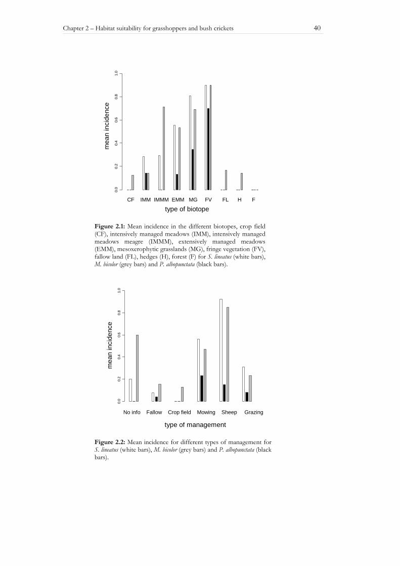
The variable ‘type of biotope’ showed a high explanatory power for all three species in single parameter models (Table 2.2). Internal validation of the single parameter model with ‘type of biotope’ as variable was successful for all three species. Transferability in time was possible for that model in all cases and for S. lineatus transferability in space could also be proven (Table 2.2). For all three species the ‘fringe vegetation’ has the highest probability of occurrence followed by mesoxerophytic grassland (Figure 2.1).
The ‘type of management’ alone did not yield high explanatory power for the spatial distribution of the species, but was included in some of the multiple models and may be important in terms of conservational aspects. For P. albopunctata mowing always correlates with a high incidence. The other two species (M. bicolor and S. lineatus) are most often found on plots under extensive sheep-grazing management (Figure 2.2). Intensively managed areas as well as areas with no management at all are avoided by all three species. Generally, the ‘type of management’ can not explain as much variation in incidence as the ‘type of biotope’.
Chapter 2 – Habitat suitability for grasshoppers and bush crickets 40
Figure 2.2: Mean incidence for different types of management for S. lineatus (white bars), M. bicolor (grey bars) and P. albopunctata (black bars).
Figure 2.1: Mean incidence in the different biotopes, crop field (CF), intensively managed meadows (IMM), intensively managed meadows meagre (IMMM), extensively managed meadows (EMM), mesoxerophytic grasslands (MG), fringe vegetation (FV), fallow land (FL), hedges (H), forest (F) for S. lineatus (white bars), M. bicolor (grey bars) and P. albopunctata (black bars).
type of habitat
mea
n in
zide
nce
0.0
0.2
0.4
0.6
0.8
1.0
CF IMM IMMM EMM MG FV FL H F
type of biotope
mea
n in
cide
nce
type of management
type of management
mea
n in
zide
nce
0.0
0.2
0.4
0.6
0.8
1.0
No info Fallow Crop field Mowing Sheep Grazing
mea
n in
cide
nce
Chapter 2 – Habitat suitability for grasshoppers and bush crickets 41
2.3.3 Additional analyses
Separate analyses for different types of biotope
The comparison of occupied and unoccupied plots carried out separately for each ‘type of biotope’ allows a closer look at habitat selection, yielding specific models for specific types of biotope. Low ‘vegetation height’, low ‘total horizontal cover’ as well as low ‘cover at the heights of 20/30/40 cm’ are attributes preferred by S. lineatus on mesoxerophytic grasslands (Mann-Whitney U test, p < 0.05 for all cases). By conducting the same analyses for M. bicolor we could not detect any significant differences between occupied and unoccupied plots (Mann-Whitney U test, p > 0.05 for all cases). P. albopunctata prefers extensively managed meadows with west-faced exposition (Mann-Whitney U test, p < 0.05 for all cases).
Microhabitat preferences and influence of surrounding type of biotope
In our study all three species did not show any significant preferences of distinct microhabitat parameters (Wilkoxon match paired test after Bonferroni correction for multiple comparisons, all comparisons p > 0.05). The surrounding in 10 m to 25 m and 25 m to 50 m did not provide additional information for the occurrence probability of M. bicolor and P. albopunctata. For S. lineatus the surrounding between 25 m and 50 m as well as the calculated values for the plot itself remained in the model after stepwise backward variable selection (AUCbootstrapped = 0.823).
2.4 DISCUSSION
2.4.1 Influence of plot characteristics on the occurrence probability of species
In our study the species with the most restricted habitat requirements was P. albopunctata. It only occurred on fringe vegetation, mesoxerophytic grasslands and intensively managed meadows with meagre parts. The two other species, M. bicolor and S. lineatus, were also found on extensively managed meadows. This result corresponds well with the literature on habitat requirements of the species (Detzel 1998).
After the reduction of the data set to those types of biotope that yielded at least some incidence, the variable ‘type of biotope’ significantly contributes to many models. It obviously has a great influence on the occurrence probability of the species. Additionally, for S. lineatus low vegetation height as well as low total horizontal cover strongly influence occurrence. This may be explained by the fact that egg development depends on temperature (van Wingerden et al. 1991) and
Chapter 2 – Habitat suitability for grasshoppers and bush crickets 42
females lay their eggs in the upper ground layer or on the button upholstery of grasses (Oschmann 1993).
For M. bicolor a south-faced exposition, high vegetation and sheep grazing are the factors that – in combination with the type of biotope – explain most of the variance in the data. For this species fringes, mesoxerophytic grasslands, as well as extensively managed meadows offer good food resources as the larvae are feeding on grasses as well as on flowers of grasses and herbs (Ingrisch 1976). This holds especially if they are managed by sheep-grazing. As males of this species are calling in higher vegetation (Detzel 1998) and females lay their eggs in grass stems (Hartley & Warne 1972) a preference for high vegetation may correspond to the vertical orientation of the species.
The occurrence of P. albopunctata is best described by the combination of the variables: ‘type of biotope’, ‘type of management’ and ‘vegetation height’ at the plots. Low vegetation height and thus increased temperature promotes the larval development of P. albopunctata (Detzel 1998). Apart from the influence of the type of biotope, management regime (i.e. man-made disturbance) contributes to habitat suitability for all three species. P. albopunctata is mostly found on mowed mesoxerophytic grasslands and fringes, which provide an elevated ground temperature, and low vegetation due to their position on the steeper, upper south-faced hillsides. The other two species preferred areas which are extensively grazed by sheep. As Detzel (1998) describes a preference for areas managed by sheep-grazing also for P. albopunctata, our result seems to be in contrast to the habitat requirements of P. albopunctata described in that study. But our result may be biased by the fact that the mesoxerophytic grasslands as well as the fringes investigated are all managed by mowing, therefore mowing and fringes cannot be separated.
Although we cannot precisely predict the best management practice for the conservation of P. albopunctata, we would like to point out that even mowed habitats may be suitable for that species. Grazing by sheep is mainly used on extensively managed meadows, where it produces a heterogeneous mosaic of high and short vegetation patches within one area (Adler et al. 2001). Such complex habitats offer a variety of different local conditions for different activities like feeding, mating or reproduction. Intensively managed, agricultural or silvicultural areas as well as abandoned areas with no management at all are avoided by all three species.
Both, the ‘type of biotope’ as well as the ‘type of management’ are proxies for the real driving factors of the incidence of grasshoppers and bush crickets. Their influence on occurrence probability is determined by a variety of different other factors (e.g. predation risk, exposition, temperature regime) that are actually relevant to the species’ survival or habitat selection. This may explain the contrasting effects of management regime for P. albopunctata. It is neither the ‘type of biotope’ nor the exact management regime that determines species occurrence,
Chapter 2 – Habitat suitability for grasshoppers and bush crickets 43
but the resulting level of the actually relevant factors (e.g. increased temperature for egg development) that determines habitat quality for the species.
The effect of spatial autocorrelation is neglected in most studies on species-habitat-relationships (but see Hinch et al. 1994, Smith 1994, Collingham et al. 2000, Osborne et al. 2001, Judas et al. 2002, Keitt et al. 2002). To avoid misleading interpretations due to inadequate degrees of freedom in significance tests we excluded models from the analyses if residuals showed spatial autocorrelation. Especially in the case of P. albopunctata this led to the exclusion of a number of models. This may be due to the fact that the species shows a clustered occurrence pattern in our region which is explained by the limited dispersal ability of the species.
Although the type of stratified random sampling used in our study is an adequate and commonly used method (see also Wessels et al. 1998, Hirzel & Guisan 2002), we would recommend to use a two step approach whenever possible for further studies. This should start with a preliminary study (which was not possible in our case) with which clear non-habitat structures can be determined to exclude these by rules from the analyses (Dufrene & Legendre 1991, Aspinall & Lees 1994). The intensive work on the detailed habitat requirements of a species can then be done in a main study with a high sample size in habitats with intermediate occupancy (see also Hirzel & Guisan 2002). Such an approach with higher sample sizes always improves the quality of the results (Hirzel & Guisan 2002). Especially in the case of the bush cricket P. albopunctata where we only had a prevalence of around 20% in the nature reserve ‘Hohe Wann’, this would most probably have improved the precision of our model. In the case of the other two investigated species prevalence was around 40 to 50 %. This is regarded as optimal for the development of logistic regression models (Hosmer & Lemeshow 2000).
2.4.2 Microhabitat preferences and influence of surrounding type of biotope
In contrast to the findings of Krätzel (1999) and Krätzel et al. (2002) for M. bicolor we did not find any evidence for the preference for distinct microstructures. This may be due to the fine-grained scale of our study. Our plots were rather small (just 225 m2) compared to the 800 – 1320 m2 in the study of Krätzel (1999) and Krätzel et al. (2002). Thus our plots may have been rather homogeneous. We would nevertheless expect that our species do actively select distinct microhabitats at a larger plot size respectively on a larger spatial scale than investigated here. This argument is supported by our separate analyses for each type of biotope which showed a clear preference for some structural aspects of occupied compared to unoccupied plots for P. albopunctata and S. lineatus.
For P. albopunctata and M. bicolor no additional influence of the plot surrounding on habitat occupancy could be detected. The plot surrounding in a radius of 25 m is highly correlated with the plots type of biotope because these area represents roughly the mean, natural patch size in the nature reserve ‘Hohe

Chapter 2 – Habitat suitability for grasshoppers and bush crickets 44
Wann’. For S. lineatus the surrounding between 25 m and 50 m was a significant variable in the model together with the plots own type of biotope. Whether this influence is based on metapopulation effects or the spatial heterogeneity of S. lineatus habitats can not be decided in this study. But an additional study covering more of the surrounding could yield more information.
2.4.3 Model validation
Validation either internally or externally is still not very common in habitat suitability model building, though it is the best possibility to really judge how robust and general a model is. For all three species the simple model including the ‘type of biotope’ as explanatory variable could be validated internally and showed a good transferability in time. For S. lineatus it also could be transferred in space. Spatial validation was not possible in all other cases eventually due to the low sample size in the second study area (28 plots) and the fact that the range of tested categories for ‘type of biotope’ and ‘management’ in the second study area was too small (see Table 2.1). In such a case it is more likely that we compared two different sampling designs rather than performing an external validation (Lehmann et al. 2002). For future studies we would recommend to use the same sampling design with similar sampling effort to perform a spatial validation of habitat suitability models. The failure of transferability in time for the multiple parameter models of M. bicolor might be caused by their instability. None of these models were stable with respect to the selected explanatory variables and only the variable ‘type of biotope’ resulted in stable models after bootstrapping with stepwise backward variable selection.
2.4.4 Conservational/Practical aspects
The type of biotope is always a powerful predictor of species occurrence if we used it as single variable or even in the reduced data sets and multiple regression analyses. Thus, we can on the one hand conclude that the type of biotope as highly integrating variable accounts for some parameters we did not estimate. On the other hand, and especially useful for nature conservation, simple vegetation type maps (type of biotope) might sometimes be sufficient to predict species occurrence with satisfactory precision. The use of these models would provide a quick and efficient possibility to determine the distribution of species under different management regimes and in other regions.
Chapter 3
The generality of habitat suitability
models: How well may grasshoppers be
predicted by butterflies?
with Birgit Binzenhöfer, Hans-Joachim Poethke, Robert Biedermann,
Josef Settele and Boris Schröder
IN PREP. FOR BASIC AND APPLIED ECOLOGY
Abstract. Knowledge of the relationship between habitat properties and the occurrence of a particular species is an essential prerequisite for the conservation of species. Habitat suitability models are one possibility to describe habitat preferences of a species quantitatively and objectively. In this study we compare the habitat preferences of different insect species (grasshoppers, bush crickets, butterflies) in the same area and with the same methods. To identify common parameters to predict occurrence probability of these species, we first tested transferability of single species models to species within the same insect group. The ‘best’ group models were then tested for transferability between the different groups. Although in the single species models different key factors have been shown to be responsible for habitat suitability, some models were successfully transferred. The habitat preferences of the moth Z. carniolica were particularly well suited for the prediction of suitable habitats for all other species. The variable ‘type of biotope’ played a dominant role in all models. With this predictor suitable habitat may be predicted for all studied species under different management regimes.


Chapter 3 – Generality of habitat suitability models
47
3.1 INTRODUCTION
Historically, arid grasslands arose due to anthropogenic influences, e.g. logging or abandonment of vineyards or fields on steep hill sides. In former times, they have most often been used as grazing sites or mowing areas. Situated mostly on nutrient poor soil or inaccessible hill sides they usually are of low agricultural productivity (Willems 1990, Van Dijk 1991) and only worked with high effort. Nowadays these semi-natural habitats are increasingly lost by either intensification (e.g. through fertilisation) or abandonment (e.g. succession by shrubs and hedges; Mühlenberg 1996, Van Dijk 1991, Poschlod et al. 1996, Kahmen et al. 2002). But because these areas simultaneously accommodate a variety of threatened and protected animal and plant species (van der Maarel & Titlyanova, Kull & Zobel 1991, Bignal & McCracken 1996), it is a declared objective of nature conservation in Europe to protect them (Bobbink & Willems 1993, Söderström et al. 2001). However, management regimes for these areas are not easily developed since maintenance depends on regular management, but species diversity is known to decline with increased management intensity (Kruess & Tscharntke 2002). Thus, a variety of different management regimes has been proposed and tested (Schreiber 1977, Bakker 1989, Bobbink & Willems 1993, Kahmen et al. 2002) including the ones from the MOSAIK-project: rototilling and extensive grazing by goats (see Fritzsch et al., Kleyer et al. this issue).
Independent of the kind of management and the time intervals between management events a certain vegetation composition or rather successional stage of the managed area can be found. This successional stage results in different levels of habitat suitability for different animal species. Which degree of succession will be advantageous for the desired ‘target species’ can be determined by describing the habitat requirements of a species with statistical habitat suitability models (Bonn & Schröder 2001, Hein et al. submitted). Different species or insect groups vary in their respective habitat needs. Therefore the resulting favoured successional stage will vary from species to species.
For the conservation of grasslands it is important to protect as many species as possible. Thus, habitat requirements of a large number of single species have to be brought together. In this context one could imagine two approaches. First, the identification of single species which are representatives for others concerning habitat requirements (New 1995, Simberloff 1998, Bonn & Schröder 2001). Secondly, the combination of single species habitat requirements to find a common set of variables relevant for the occurrence of a maximum number of species. Both methods would make it feasible to predict suitable habitats and the impact of different management types on the occurrence of more than one species.

Chapter 3 – Generality of habitat suitability models
48
Within the MOSAIK project the habitat requirements of different insect species have been studied separately (Binzenhöfer et al. in prep., Hein et al. submitted, Strauß et al. in prep.). In this study we compare results of these analyses for three different Orthoptera (Ensifera: Metrioptera bicolor, Platycleis albopunctata, Caelifera: Stenobothrus lineatus ) and two butterfly species (Lepidoptera: Coenonympha arcania, Zygaena carniolica) typically found on semi-arid grasslands and tested whether the inclusion of factors delivered by a digital terrain model and a landscape model (see Schröder et al. this issue) increases their predictive power. For the resulting single species models we will first test transferability within the species of one insect group (within group transfer). The resulting ‘group’ models are then transferred to the other groups (between group transfer; Bonn & Schröder 2001). Additionally, for the determination of a representative or ‘umbrella’ species we tested whether the incidence of one species can be used to predicted incidences of others just as well (Hanley & McNeil 1983, Bonn & Schröder 2001).
3.2 MATERIAL AND METHODS
This study is based on data from different authors (Binzenhöfer et al. in prep., Hein et al. submitted, Strauß et al. in prep.). All studies used the same experimental design to achieve comparable data sets for the different species. To keep this section short, we would like to refer to the original papers for a detailed description of data collection and characterization of the experimental plots (Binzenhöfer et al. in prep., Strauß et al. in prep., Hein et al. submitted). In cases were analyses differed in the original papers we adjusted all analyses to the methods presented in Binzenhöfer et al. (in prep.) and Strauß et al. (in prep.).
3.2.1 The species
Grasshoppers and bush crickets
The stripe-winged grasshopper Stenobothrus lineatus (PANZER 1796; Orthoptera: Acrididae), the two-coloured bush cricket Metrioptera bicolor (PHILIPPI 1796; Orthoptera: Tettigoniidae) and the grey bush cricket Platycleis albopunctata (GOEZE 1778; Orthoptera: Tettigoniidae) are classified as thermo- and xerophilic (Harz 1969, Detzel 1998, Ingrisch & Köhler 1998). They typically inhabit arid and semi-arid grasslands as well as broom and juniper heath. S. lineatus and P. albopunctata are also found on fringes and areas with open soil and sparse vegetation. In contrast M. bicolor is more orientated towards vertical structures and thus prefers long lawn biotopes. For S. lineatus sheep-grazed areas and short vegetation structure are preferred habitat elements (Detzel 1998). In general,
Chapter 3 – Generality of habitat suitability models
49
P. albopunctata has a more narrow distribution in Germany than the other two species.
Butterflies and moths
The flight period of the Pearly Heath Coenonympha arcania (LINNAEUS 1761; Satyridae: Satyrinae) lasts from end of May till beginning of August. Generally this species is univoltine (Ebert & Rennwald 1991, Hensle 1995). Imagines are found on mesoxerophytic grasslands with bushes in the near vicinity of hedges and forest edges (Ebert & Rennwald 1991, Weidemann 1995, Settele et al. 1999). Caterpillars feed preferentially on Holcus lanatus, Brachypodium pinnatum, Festuca ovina or Melica spec. (Ebert & Rennwald 1991, Weidemann 1995).
The day active moth Zygaena carniolica (SCOPOLI 1763; Lepidoptera: Zygaenidae) has a flight period of four to five weeks from the end of June to mid August (Ebert & Rennwald 1991). This xerothermophilic species (Ebert & Rennwald 1991) inhabits mainly fallow as well as extensively grazed or mowed mesoxerophytic grasslands (Ebert & Rennwald 1991, Weidemann 1995). Preferred caterpillar feeding plants are Onobrychis viciifolia and Lotus corniculatus. Imagines prefer purple flowering nectar plants like Knautia arvensis, Scabiosa columbaria and Centaurea spec. (Ebert & Rennwald 1991, Weidemann 1995).
3.2.2 Field work
All studies were conducted in the field seasons of 2001 and 2002 in the nature reserve ‘Hohe Wann’ in Northern-Bavaria, Germany (latitude 50° 03′, longitude 10° 35′). The study area is characterised by abundant sites of mesoxerophytic grasslands, formerly used as vine yards (Elsner 1994). These patches are separated by agricultural landscape of different use. The whole area covers approximately 10 km in NS-direction and 4 km in EW-direction.
Incidence of the species under study was recorded on 146, 139 and 106 experimental sites for orthoptera, Z. carniolica and C. arcania respectively. Experimental plots were selected by stratified random sampling across the ten main types of biotope occurring in the region. To increase the resolution of the logistic regression models we sampled with high effort in habitats with - based on prior knowledge – uncertain status regarding the species’ occurrence (i.e. different kinds of open grasslands). To assure comparability of results the study plots of the grasshoppers and bush cricket studies (15 m x 15 m) were always a randomly chosen corner of the butterfly/moth plots (30 m x 30 m). Different plot sizes were chosen as butterflies/moths are more mobile than grasshoppers or bush crickets.
For the determination of grasshopper, bush cricket, butterfly and moth incidence we carried out transect sampling on the experimental sites. The census was terminated (i) as soon as a specimen was found or (ii) after a maximum of 15 minutes (butterflies, moths) or 20 minutes (grasshoppers, bush crickets) of

Chapter 3 – Generality of habitat suitability models
50
sampling time. As the activity of grasshoppers, bush crickets, butterflies and day active moths strongly depends on weather conditions, censuses were only carried out during ‘good’ weather condition (sunshine, cloud cover < 3/8; air temperature > 17 °C; wind speed < 4 m/s (Mühlenberg 1993)) to ensure the same detection probability on all plots.
3.2.3 Statistical analyses
Single species models
We used single and multiple parameter logistic regression to determine the impact of ‘landscape’ factors delivered by the digital terrain model and landscape model (like solar radiation, slope, soil type, geology, Schröder et al. this issue) on the occurrence probability of all studied insect species (Manel et al. 1999a, b, Hosmer & Lemeshow 2000). For the selection of adequate models we started with an univariate analysis to assess indiviudal model variables independently from each other (Hosmer & Lemeshow 2000). To choose uncorrelated parameters for the development of multiple parameter models we calculated all pairwise Spearman rank correlations and selected only one variable of those pairs showing severe correlation (ρs ≥ 0.5; Fielding & Haworth 1995, Schröder 2000). Only parameters with p-values < 0.2 (Hosmer & Lemeshow 2000) were included into multiple analyses.
For model evaluation we used Nagelkerkes R2 value (Nagelkerke 1991, Harrell 2001). Model discrimination was assessed by the threshold independent AUC-value, i.e. the area under the receiver operating characteristic curve (ROC-curve), the (Hanley & McNeil 1983, Hosmer & Lemeshow 2000, Schröder 2000, Manel et al. 2001). Variables with an AUC-value > 0.7 were included into the models from the single species studies and their importance was tested with the stepwise backwards elimination procedure.
For comparison of the resulting models with the same dependent variable we used the Akaike Information Criterion (AIC, see also Buckland et al. 1997, Augustin et al. 2001), which allows to choose the model with the optimal compromise between goodness of fit and the lowest number of parameters. Models with the lowest AIC were tested for spatial autocorrelation by calculating Moran’s I as an index of covariance between different point locations (Lichstein et al. 2002, Karagatzides et al. 2003). Only models without spatial autocorrelation were used for further analyses and internally validated by applying a bootstrapping procedure (Verbyla & Litvaitis 1989, Reineking & Schröder 2003). For internal validation we first calculated the AUC value of the full model with 300 bootstrap samples and then tested for stability of the model with variable selection by using the backward stepwise approach with α = 0.05 and 300 bootstrap samples (see also Oppel et al. in press).

Chapter 3 – Generality of habitat suitability models
51
Test of transferability
Each of the single species models was tested for transferability in two ways. First, the model was computed for the species it was developed for. Then predicted occurrence probabilities for that species were used to predict the occurrence of the other species (Hanley & McNeil 1983).
Secondly, we tested transferability by using the parameters from the ‘best’ model for species A and calculating a new model with these parameters based on the incidence of species B. In both cases agreement between predictions and occurrences are tested by comparing the AUC value with an AUCcrit ≥ 0.5 (ROC-tool available at http://brandenburg.geoecology.uni-potsdam.de/users/schroeder /download.html by Schröder B.). The transfer quality of a model is best when all possible combinations result in significantly better AUCs than 0.5. For within group comparisons of transferability this methods result in five possible combination for the three orthoptera species, respectively in three combinations for the two butterfly species. The highest possible number of successful transfers of a single species model for between group comparisons is seven.
The ‘type of biotope’ or derivates of this parameter were included in all single species models. Additionally, this parameter is landscape wide available. Thus, we tested the ‘type of biotope’ of the experimental plot of grasshopper and bush cricket incidences, which corresponds in most cases to the main type of biotope on all experimental plots, for its prediction ability. Thereby, its transferability was tested between species (25 possibilities for combination).

Chapter 3 – Generality of habitat suitability models
52
3.3 RESULTS
3.3.1 Single species models
The univariate analyses of the ‘landscape’ factors from the digital terrain and the landscape model (Schröder et al. this issue) resulted in an influence of slope, solar radiation, disturbance intensity, management, geology and soil type on the occurrence probability of grasshopper, bush crickets and butterfly species. For the studied butterfly species, the grasshopper S. lineatus as well as for the bush cricket M. bicolor inclusion of these parameters in the so far best single species models did not result in new models as the parameters were eliminated during stepwise backward procedure (Table 3.1). Only for the bush cricket P. albopunctata inclusion of the parameter ‘solar radiation’ resulted in new models with lower AIC than the one presented by Hein et al. (submitted; Table 3.1).
Table 3.1: Single species models with model characteristics (AUC with SE, R 2Nagelkerke, AIC, AUCbootstrapped after internal validation with backwards variable selection) for the five investigated species (p < 0.05).
Species model parameter AUC R 2Nagelkerke
AIC AUCbootstrapped
S. lineatus type of biotope
vegetation height (quadratic term)
0.762 0.367 115.92 0.735
M. bicolor suitable habitat in r = 50 m (i.e. fringes, mesoxerophytic grassland,
extensively managed meadows) 0.740 0.227 117.94 0.723
P. albopunctata
sinus exposition vegetation height
solar radiation proportion fringes in r = 75m
0.949 0.712 40.84 0.941
C. arcania
time of first management incidence tree layer
proportion mesoxerophytic & extensively managed grassland in
r=100m proportion hedges on suitable
area in radius=25m
0.94 0.7 92 0.9
Z. carniolica
Incidence Centaurea jacea Incidence Scabiosa columbaria
Suitable types of biotope in radius = 25m
(i.e. fringes, mesoxerophytic grassland, extensively managed grassland)
0.92 0.6 94 0.911
For all three orthoptera species the ‘fringe vegetation’ has the highest
probability of occurrence followed by mesoxerophytic grassland. In addition, low vegetation height increases occurrence probability of S. lineatus. For P. albopunctata
Chapter 3 – Generality of habitat suitability models
53
habitat suitability decreases with increasing vegetation height, increasing solar radiation and west faced exposition (Table 3.1).
The occurrence probability of C. arcania is positively influence by late ‘time of first management’ and an existing ‘tree layer’ (Table 3.1). Additionally, a high ‘proportion of mesoxerophytic grassland and extensively managed meadows in the radius of 100 m’ and a high ‘proportion of hedges on suitable habitat in the radius of 25 m’ increase the occurrence probability of the species. The highest probability of occurrence for Z. carniolica is predicted for areas with a high proportion of mesoxerophytic grasslands, fringes and extensively managed meadows (indicated by the inclusion of the variable ‘proportion of suitable habitat in a radius of 25 meter’). Additionally, the occurrence of Scabiosa columbaria and Centaurea jacea contributed to the model (Table 3.1).
3.3.2 Test of transferability
For grasshoppers and bush crickets transferability of a single species model within group was best conducted with the model of S. lineatus including the variables ‘type of biotope’ and ‘vegetation height’ (Table 3.2). The occurrence of C. arcania and Z. carniolica is best predicted by the model of Z. carniolica (Table 3.2). Hereby, the proportion of suitable habitat (fringes, mesoxerophytic grassland, extensively managed grassland) in a radius of 25 m as well as the occurrence of the sucking plants Centaurea jacea and Scabiosa columbaria are explaining variables in the model.
Table 3.2: Results of within group transfers. For orthoptera the model of S. lineatus, including the variables ‘type of biotope’ and ‘vegetation height’ showed the best transferability (five successful out of five possible transfers). For butterflies the model of Z. carniolica, including ‘suitable habitat in r = 25 m’ and occurrence of C. jacea and S. columbaria was best transferable. AUCs significantly exceeding an AUCkrit = 0.7 are indicated by **, those significantly exceeding an AUCkrit = 0.5 by *. Original models are marked in grey.
Model outcome - transferability Independent variables from the model of species
Species incidence used
for model calibration
Species incidence to be predicted AUC Lower…upper
confidence bounds
S. lineatus 0.762* 0.677…0.848 M. bicolor 0.632* 0.525…0.739 S. lineatus
P. albopunctata 0.870** 0.794…0.946 M. bicolor M. bicolor 0.771* 0.68…0.862
S. lineatus
P. albopunctata P. albopunctata 0.868** 0.788…0.948 Z. carniolica 0.919** 0.870…0.969
Z. carniolica C. arcania 0.613* 0.507…0.719 Z. carniolica
C. arcania C. arcania 0.898** 0.837…0.960
In the between group transfer the model of Z. carniolica performs slightly
better than the one from S. lineatus (one more successful transfer; Table 3.3). The independent variable ‘type of biotope’ showed the highest transferability to all species, with 100 % (=25/25) successful transfers (Table 3.4).

Chapter 3 – Generality of habitat suitability models
54
Table 3.3: Results of between group transfer with the butterfly ‘group’ model (Z. carniolica). AUCs significantly exceeding an AUCkrit = 0.7 are indicated by **, those significantly exceeding an AUCkrit = 0.5 by *. Original models are marked in grey.
Model outcome - transferability Independent variables from the model of
species
Species incidence used
for model calibration
Species incidence to be predicted AUC Lower…upper
confidence bounds
Z. carniolica 0.919** 0.870…0.969 S. lineatus 0.760* 0.681…0.839 M. bicolor 0.766* 0.681…0.839
Z. carniolica
P. albopunctata 0.738* 0.650…0.826 S. lineatus S. lineatus 0.775* 0.688…0.862 M. bicolor M. bicolor 0.747* 0.659…0.835
Z. carniolica
P. albopunctata P. albopunctata 0.787* 0.674…0.9
Table 3.4: Results of tests of transferability with the independent variable ‘type of biotope’ from 15m x 15m experimental plots. AUC significantly exceeding an AUCkrit = 0.7 are indicated by **, those significantly exceeding an AUCkrit = 0.5 by *. Models representing a single species model are marked in grey.
Model outcome - transferability Independent
variable
Species incidence used for model
calibration
Species incidence to be predicted AUC
Lower…upper confidence
bounds
S. lineatus 0.846** 0.787…0.904 M. bicolor 0.802** 0.734…0.870
P. albopunctata 0.846** 0.769…0.922 Z. carniolica 0.803** 0.727…0.880
type of biotope S. lineatus
C. arcania 0.711* 0.624…0.799 S. lineatus 0.842** 0.780…0.904 M. bicolor 0.806** 0.739…0.873
P. albopunctata 0.842** 0.762…0.922 Z. carniolica 0.807** 0.734…0.879
type of biotope M. bicolor
C. arcania 0.736* 0.650…0.821 S. lineatus 0.807** 0.740…0.873 M. bicolor 0.766* 0.693…0.839
P. albopunctata 0.855** 0.785…0.925 Z. carniolica 0.777* 0.696…0.859
type of biotope P. albopunctata
C. arcania 0.678* 0.589…0.766 S. lineatus 0.847** 0.785…0.910 M. bicolor 0.803** 0.73…0.877
P. albopunctata 0.840** 0.773…0.906 Z. carniolica 0.82** 0.754…0.887
type of biotope Z. carniolica
C. arcania 0.745* 0.659…0.831 S. lineatus 0.773* 0.692…0.854 M. bicolor 0.762* 0.68…0.845
P. albopunctata 0.832** 0.756…0.907 Z. carniolica 0.770* 0.696…0.844
type of biotope C. arcania
C. arcania 0.811** 0.741…0.880
Chapter 3 – Generality of habitat suitability models
55
3.4 DISCUSSION
3.4.1 Single species models
The univariate logistic regression analyses with the ‘landscape’ parameters derived from the digital terrain and landscape model (Schröder et al. this issue) resulted in significant models for all species. But none of these parameters is included in the multiple parameter models for S. lineatus, M. bicolor, Z. carniolica and C. arcania. Only the occurrence probability of P. albopunctata increased significantly with the inclusion of the factor solar radiation in the multiple parameter logistic regression models. This is in agreement with the high temperature requirements of this species for egg and larval development. Based on this results one may conclude that disturbance factors like disturbance frequency or intensity have no influence on habitat suitability for our species. We consider this a very unlikely situation. Especially, adult butterflies are sensitive to changes in temperature, light and humidity levels, parameters that are often affected by habitat disturbance (Wood & Pullin 2002). We assume that this result is better explained by the fact that other factors already included in the models contain the effects of disturbance or other ‘landscape’ parameters. For example the type of biotope may be such a factor, e.g. extensively and intensively managed meadows differ in the degree of management frequency.
The proportion of suitable habitat (fringes, mesoxerophytic and extensively managed grasslands) in a radius of 25 m around the experimental plots influences occurrence probability of butterflies. This circle covers an area twice as large as the experimental plot size of 30 m x 30 m, but within the natural size of fringes and mesoxerophytic grasslands in the nature reserve ‘Hohe Wann’. This might stem from the fact that based on their high mobility habitat selection of butterflies takes place at a larger scale than the experimental plot size. On the other hand, the ‘type of biotope’ at our experimental plot should be highly correlated with the surrounding in 25 m, so that we could trace our result back to a technical reason. ‘Type of biotope’ represents a categorial variable in contrast to the metric variable ‘suitable habitat in r = 25 m’, which results in a decrease in degrees of freedom and thus increased model performance. This fact may also contribute to the exclusion of the ‘type of biotope’ and inclusion of the proportion of ‘suitable habitat’ in radii of 50 and 75 m in the model of M. bicolor respectively P. albopunctata as well. We can not easily differentiate between a technical failure or a real influence of the surrounding. Nevertheless, the composition of nearby habitats in the surrounding landscape will also affect the suitability of local habitat patches and thus population viability. For example, insects may utilise multiple habitat types during their life cycle (Noss 1990, Dunning et al. 1992, Villard et al. 1999, Sönderström & Pärt 2000) or they need to
Chapter 3 – Generality of habitat suitability models
56
disperse between habitat patches. This depends on the quality of habitats in the surrounding landscape as well (Bennett et al. 1994, Roland et al. 2000).
3.4.2 Test of transferability
Models based on the incidence of C. arcania can not be applied to other species. Additionally, the incidence of C. arcania can only be badly predicted by other species’ occurrences. This may be due to the comparatively euryoceous properties of C. arcania. C. arcania is mesophilic, e.g. its habitats cover a broad range of types of biotopes. Habitats suitable for Z. carniolica and the investigated grasshopper and bush cricket species only cover a small part of habitat suitable for C. arcania. Vice versa only a small number of C. arcania habitats are suitable for the other species.
Occurrence probabilities of all five species studied can be best predicted with the model of the moth Z. carniolica. This species may thus act as representative or ‘umbrella species’ for others. However, this needs further investigations. In the models the variable ‘type of biotope’, vegetation height and the occurrence of the sucking plants C. jacea and S. columbaria play an important role. Thereby the two plant species may not directly influence grasshoppers and bush crickets but maybe they are indicators for extensively managed areas, which are preferred by the species.
Generally, stenoecious but mobile species may be best suited as ‘umbrella’ species (New 1995). They exactly represent habitat requirements of species typically found in specific habitats and can reach all potential habitats better than species with low mobility. Although one would expect that based on their higher mobility the moth Z. carniolica is much better suited as representative species for xerothermophilic species living on semi arid grasslands, in our case the transferability of the model of the moth Z. carniolica did only differ slightly (in one more successful transfer) from the one of the grasshopper S. lineatus. This may be due to the fact that mobility is not a decisive factor for the survival of this species in the nature reserve ‘Hohe Wann’, as connectivity is probably very high for S. lineatus. To really quantify this argument a landscape wide mapping of S. lineatus for the determination of connectivity would be necessary. Alternatively, one could test and compare the predictive quality of both models in other landscapes.
In general, the parameter ‘type of biotope’ showed a high potential for the prediction of species occurrence. Particularly, the models of the grasshopper S. lineatus, the bush cricket M. bicolor as well as the moth Z. carniolica can predict occurrence of the other species very well. This result may be of outstanding practical value, particularly in conservation biology, as the ‘type of biotope’ can be relatively easy determined in contrast to costly analyses of disturbance or vegetation structure and composition. Additionally, information on the type of biotope already exists for many regions of conservational interest. The type of biotope seems to reflect an aggregation of different parameters ranging from geological prerequisites (i.e. soils, slope) to anthropogenic influences

Chapter 3 – Generality of habitat suitability models
57
(disturbance). Most importantly, it obviously also represents the perception of the environment by insect species. With reference to the MOSAIK project a prediction of the kind of type of biotope resulting from different management regime, e.g. by botanical analyses (Fritsch et al. this issue, Kühner & Kleyer this issue), would allow for a classification of suitable and unsuitable areas for threatened species according to the type of management.


Chapter 4
Movement patterns of Platycleis albopunctata in different types of habitat:
matrix is not always matrix
with Julia Gombert, Thomas Hovestadt and Hans-Joachim Poethke
ECOLOGICAL ENTOMOLOGY (2003) 28, 432-438
Abstract. Inter-patch movement is usually assumed to be homogeneous across a landscape. As the intervening area between suitable patches is usually richly textured, it cannot be assumed to be uniform in real landscapes. In an experimental mark-and-re-sight study, the movement behaviour of the bush cricket Platycleis albopunctata in four habitat types as well as at the border between two of these habitat types was observed. Analysis of recapture data indicated differences in mortality risk (or emigration rates) between habitat types. When released at the border between suitable habitat and a crop field, Platycleis albopunctata did not show a consistent preference for the suitable habitat. This suggests that the crop field is at least temporarily attractive for Platycleis albopunctata. Movement in suitable habitat was not always different from movement in the matrix, and movement between different types of matrix also differed. The results indicate that the movement behaviour of Platycleis albopunctata is influenced not only by suitability for breeding but also by structural resistance as well as other factors (e.g. food availability or habitat-specific mortality risk).

Chapter 4 – Movement patterns of Platycleis albopunctata 61
4.1 INTRODUCTION
The progressive exploitation of landscapes leaves many (insect) populations fragmented into metapopulations (i.e. small local populations not capable of long-term survival without interactions with neighbouring populations; Ehrlich et al. 1980, Hanski 1994a, b, Thomas & Hanski 1997). In such cases, the balance between extinction and colonisation of vacant patches determines the regional survival of species (Levins 1969, Hanski 1994a, b, Hanski & Thomas 1994, Hill et al. 1996). Inter-patch dispersal of individuals is the key factor determining colonisation probability and has been investigated intensively in theory (Hanski 1994a, b, Hanski & Thomas 1994, Gustafson & Gardner 1996, Hill et al. 1996, Hovestadt et al. 2000, 2001, Poethke & Hovestadt 2002) and practice (butterflies: Baguette & Nève 1994, Hanski et al. 1994, Hill et al. 1996, Kuussaari et al. 1996, Nève et al. 1996, Brommer & Fred 1999, Conradt et al. 2000, Roland et al. 2000, Matter & Roland 2002, Menéndez et al. 2002, beetles: Crist et al. 1992, Wiens et al. 1993, 1997, With et al. 1999, Roslin 2000, crickets: Riegert et al. 1954, Baldwin et al. 1958, Kindvall et al. 1998, Kindvall 1999).
Euclidian distance between suitable habitat patches and the species specific dispersal capacity are usually assumed to determine colonisation probability (Hanski 1994a, b). In general, movement of individuals in the matrix is supposed to be random or linear, but at least homogeneous across a landscape (Hanski 1994a, b, With & King 1999, Zollner & Lima 1999b). This is a simplifying but unavoidable assumption (Franklin 1993) because only few detailed studies of movement behaviour of insect species in unsuitable habitat are available. A small number of empirical studies has shown that movement behaviour differs between habitat and matrix (Wiens et al. 1997, Schultz 1998, Kindvall 1999). In these studies, movement has been investigated in only two habitat types, however landscapes, especially those dominated by anthropogenic influences, are often mosaics of a broad variety of habitat types (Kindvall 1999, Wiens 2001). Ricketts (2001) investigated the resistance of three habitat types for butterfly dispersal using a mark-recapture study, however there are very few data on how insects move in such heterogeneous landscapes. This may be due, in part, to the fact that individuals are hard to follow over longer distances (Gaines & Bertness 1993, Zollner & Lima 1999a). Knowledge of movement rules could be used in simulation models to generate more accurate predictions on the species-specific dispersal capacity and thus on survival probabilities of species in complex landscapes (Kindvall 1999).
In the work reported here, the movement behaviour of the bush cricket species Platycleis albopunctata was investigated in four habitat types. One of these areas was considered to represent suitable habitat allowing for successful reproduction for the species, the other three areas were assumed to be unsuitable
Chapter 4 – Movement patterns of Platycleis albopunctata 62
for this purpose (according to, for example, Harz 1969, Detzel 1998). Individually marked adult P. albopunctata were released in these areas and their movement behaviour was recorded and analysed to evaluate whether individuals differentiated between the habitats, whether movement behaviour differed between suitable and unsuitable (matrix) habitats, and whether movement behaviour differed between unsuitable (matrix) habitats. Generally, dispersal by flight cannot be excluded for P. albopunctata, however this is not documented and methodologically it is nearly impossible to investigate. Thus, this study was confined to dispersal on foot.
4.2 MATERIAL AND METHODS
4.2.1 The species
The grey bush cricket Platycleis albopunctata (Goeze) (Orthoptera, Tettigoniidae) is a medium-sized to large bush cricket species (18–22 mm). It is classified as a thermo- and xero-philic species (Harz 1969, Ingrisch & Köhler 1998), which inhabits dry locations, especially dry grassland as well as habitats with similar structure (Detzel 1998). Open soil, sparse vegetation, and fringes are preferred habitat elements.
The grey bush cricket is assumed to be a relatively mobile species (Detzel 1998). A mark-recapture study by Walter (1992) showed that most of the marked individuals were recaptured in a radius of 50 m, but some individuals moved > 100 m in a single day. Flight studies in a wind channel demonstrated the capability of some individuals to fly continuously for ≥ 15 min. This flight time would correspond to distances between 2 and 3 km (Gottschalk 1997), but observations of flying individuals are not documented in the literature.
4.2.2 Field work
The study was conducted in July and August 2001 in the Hohe Wann nature reserve in Northern Bavaria, Germany (50° 03′ N, 10° 35′ E). The study area is characterised by a patchwork of vegetation caused by the geological and geomorphological heterogeneity of the area and a variety of small-scale microclimatic differences due to different exposure and inclination. Agricultural fields are usually very small. The most obvious characteristic of the nature reserve is mesoxerophytic grassland (Elsner 1994).
For all experiments, individuals of Platycleis albopunctata were marked individually with a coloured point code on the pronotum and a numbered reflective tape was fixed on the femur (cf. Heller & von Helversen 1990, Samietz & Berger 1997, Kindvall 1999). This technique allows easy detection of

Chapter 4 – Movement patterns of Platycleis albopunctata 63
individuals at night (using a head lamp) and produces very high re-sight rates (> 80%; Heller & von Helversen 1990, Kindvall 1999). Before and after marking, individuals were kept in a cooling box to reduce potential handling trauma (Stettmer 1996).
4.2.3 Re-sight rates
Re-sight rates make it possible to estimate mortality risk, detection error, and quality of the marking method. In addition to the findings about individuals, findings of lost reflective tape were recorded. Tape could either be lost accidentally or be left by predators feeding on crickets. Individuals that were not found on one day, but re-sighted on one of the following days (discontinuously found individuals), were probably overlooked and allow an estimation of the detection error during the experiment. Individuals that were lost until the end of the observation period, were assumed to be either dead or to have emigrated.
4.2.4 Movement behaviour depending on habitat type
In order to test whether the movement behaviour of P. albopunctata varies with habitat type, a mesoxerophytic grassland (4000 m2) representing a suitable breeding habitat and three sites considered unsuitable (Detzel 1998) were selected as experimental sites: (1) a bare, harvested crop field (40900 m2), (2) fallow land (a former crop field lying fallow for 2 years) (22500 m2), and (3) a rich meadow (15800 m2). In all three cases, there were no suitable habitats in the near vicinity (closer than 400 m). Vegetation structure parameters and abiotic factors characterising the four experimental areas were measured in eight 1 x 1 m census plots along two transects across each of the experimental areas (Table 4.1). Vegetation structure estimates were measured according to Sundermeier (1999).
Table 4.1 Characteristic vegetation-structure and abiotic parameters on the four experimental areas. Mean values ± SD of eight censuses for each experimental site are shown.
Type Exposure Inclination
(°) Vegetation height (cm)
Total vegetation cover (vertical)
(%)
Vegetation cover (horizontal) up to
10 cm (%) Mesoxerophytic
grassland S 33 ± 24 29 ± 13 97 ± 3 58 ± 26
Harvested crop field
none 0 0 48 ± 19 0.6 ± 0.4
Rich meadow NE 14 ± 4 11 ± 3 90 ± 5 83 ± 8 Fallow land SE 13 ± 10 12 ± 6 81 ± 12 60 ± 16
In each area, 46 individuals of Platycleis albopunctata (23 males, 23 females) were released at randomly chosen points within 6 m of the centre of the experimental area. Individuals were released in the afternoon, singly, next to numbered wooden sticks. In the following 6 nights, the position of each re-sighted individual was recorded. A 24-h observation interval was chosen because
Chapter 4 – Movement patterns of Platycleis albopunctata 64
bush crickets and grasshoppers are known to be stationary most of the time and to move only occasionally between different sites on a small spatial scale (With 1994a).
Comparison of daily movement distances among the 6 observation days showed that distances covered on the first day in the three unsuitable habitats were significantly shorter than on the following days (Wilkoxon matched paired test, p < 0.05). This is probably due to the fact that individuals did not have a 24 h time interval between release and observation on the first day compared with the following observation days. The data from the first day were therefore excluded from further analysis.
4.2.5 Edge-mediated behaviour
In order to investigate whether individuals showed a preference for suitable habitat, 50 individuals (25 males, 25 females) were released directly along the border between a harvested crop field and a mesoxerophytic grassland (suitable habitat). The distance between the release points was 1 m. Release points were marked with numbered wooden sticks. In the following 2 nights, it was recorded whether individuals moved into the mesoxerophytic grassland, into the crop field, or stayed at the border (within a 1 m corridor along the edge). From these values, edge permeability P(out) was calculated as the proportion of observed individuals that moved into the crop field (Kindvall 1999). To account for the potential influence of handling on behaviour immediately after release, data were recorded on the 2 consecutive nights after the release of individuals in late afternoon.
For all experiments, individuals of Platycleis albopunctata were caught in habitats ≥ 850 m from the experimental sites, in order to equalise the treatment effect of removal in the four different habitat types. All individuals involved in this study were captured in the field on the day of the experiment.
4.2.6 Statistical analyses
Data analysis was complicated by the fact that not all individuals were found continuously in the 6 observation nights. This resulted in an incomplete capture history and left three different possibilities for data analysis: (1) The most conservative decision would be to take only the data from individuals found (continuously) throughout the whole period. This would have the advantage of analysing only unambiguously documented data without making assumptions about the days missing in the record; however this approach reduces the amount of data available for interpretation severely. Only the data from the first 4 days would provide sufficiently high sample numbers to merit statistical analysis. (2) Another way to analyse the data would have been to replace missing data by calculated mean values. In that case, all measured data could be used for the analysis, however this may lead to a wrong interpretation und underestimation of
Chapter 4 – Movement patterns of Platycleis albopunctata 65
true values, especially in the case of daily movement distances. (3) The alternative chosen was to use all data resulting from measurements during 2 consecutive days, even if the record was previously interrupted. In this case, the sample size was sufficiently high and the risk of underestimating daily movement distances could be avoided.
All data were tested for normal distribution and variance homogeneity using the Kolmogorov-Smirnov and Levene tests. As most of the data were not distributed normally, Kruskal-Wallis H tests were needed for comparison of more than two independent samples, and Mann-Whitney U tests for two independent samples were applied. The Kolmogorov-Smirnov Z test was used for comparison of frequency distributions of daily movement distances on the four experimental areas. As the Kolmogorov-Smirnov Z test is a test for two samples, the results for multiple comparisons were corrected by applying the sequential Bonferroni method (Rice 1989). Daily movement distances on one experimental area were tested for variation between days using a Friedmann test and Wilkoxon matched paired tests as data were not independent of each other. The Rayleigh test was used to test for a uniform distribution of circular data. Rayleigh's uniformity test calculates the probability of the null hypothesis that the data are distributed in a uniform manner.
4.3 RESULTS
4.3.1 Re-sight rates
The fate of marked individuals and markings over time on the four experimental sites are shown in Figure 4.1. Mean re-sight rates were highest for the crop field and the mesoxerophytic grassland where day-to-day re-sight rates were > 80% during the whole experimental period. In the two other experimental areas, the loss of individuals (mortality and/or emigration) was higher, but day-to-day re-sight rates were still > 75% on the fallow land and > 60% on the rich meadow. Re-sight rates during the edge experiment were > 80% on both observation days. The proportion of individuals that was not re-sighted continuously remained nearly constant (between 4 and 9%) during the observation period and for all experimental sites.
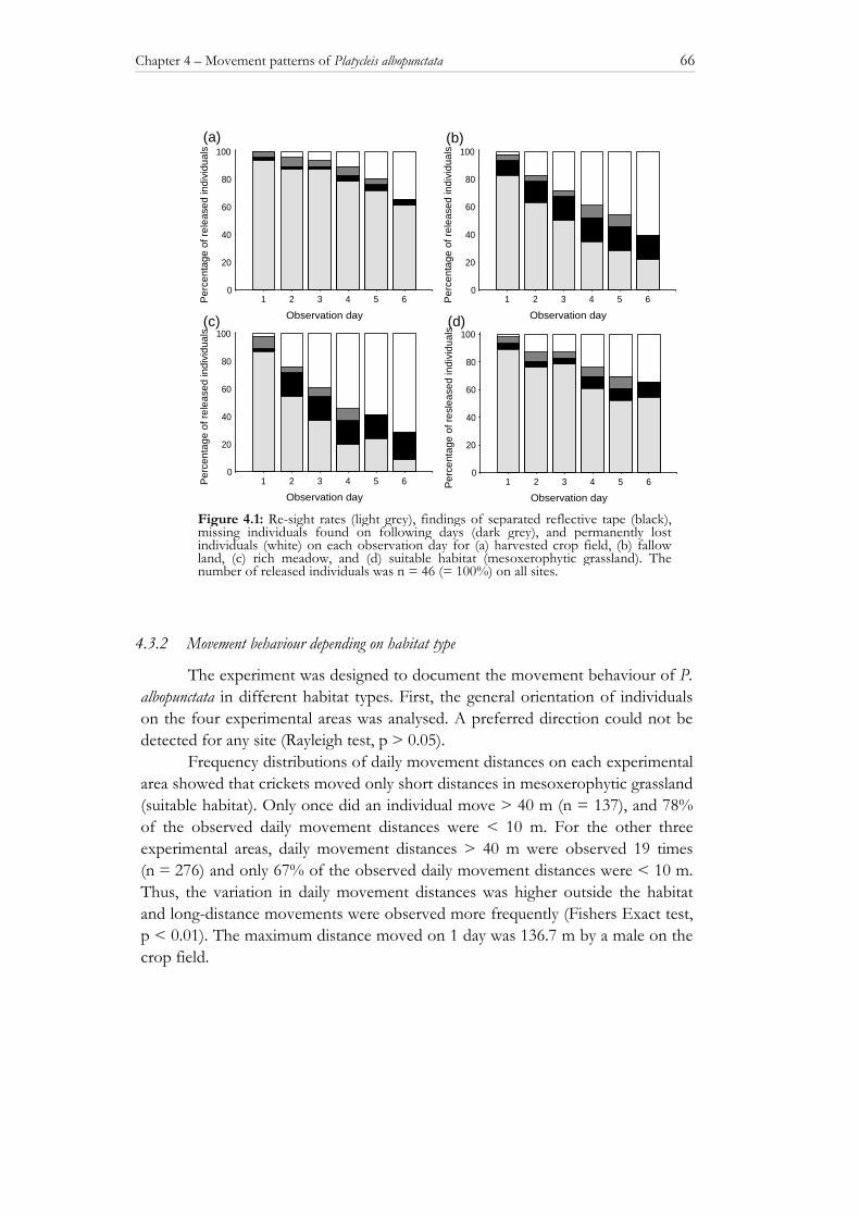
Chapter 4 – Movement patterns of Platycleis albopunctata 66
4.3.2 Movement behaviour depending on habitat type
The experiment was designed to document the movement behaviour of P. albopunctata in different habitat types. First, the general orientation of individuals on the four experimental areas was analysed. A preferred direction could not be detected for any site (Rayleigh test, p > 0.05).
Frequency distributions of daily movement distances on each experimental area showed that crickets moved only short distances in mesoxerophytic grassland (suitable habitat). Only once did an individual move > 40 m (n = 137), and 78% of the observed daily movement distances were < 10 m. For the other three experimental areas, daily movement distances > 40 m were observed 19 times (n = 276) and only 67% of the observed daily movement distances were < 10 m. Thus, the variation in daily movement distances was higher outside the habitat and long-distance movements were observed more frequently (Fishers Exact test, p < 0.01). The maximum distance moved on 1 day was 136.7 m by a male on the crop field.
Observation day
Per
cent
age
of r
elea
sed
indi
vidu
als
1 2 3 4 5 60
20
40
60
80
100
Observation day
Per
cent
age
of r
elea
sed
indi
vidu
als
1 2 3 4 5 60
20
40
60
80
100
Observation day
Per
cent
age
of r
elea
sed
indi
vidu
als
1 2 3 4 5 60
20
40
60
80
100
Observation day
Per
cent
age
of r
esle
ased
indi
vidu
als
1 2 3 4 5 60
20
40
60
80
100
(a) (b)
(c) (d)
Figure 4.1: Re-sight rates (light grey), findings of separated reflective tape (black), missing individuals found on following days (dark grey), and permanently lost individuals (white) on each observation day for (a) harvested crop field, (b) fallow land, (c) rich meadow, and (d) suitable habitat (mesoxerophytic grassland). The number of released individuals was n = 46 (= 100%) on all sites.

Chapter 4 – Movement patterns of Platycleis albopunctata 67
To compare daily movement distances on the four habitats, a mean value for each individual was calculated, resulting in independent values for each area (see also Haddad 1999). These calculated mean values of daily movement distances in the mesoxerophytic grassland and the rich meadow were significantly shorter than those in the crop field and the fallow land (Mann Whitney U test, p < 0.05; Figure 4.2). The distance between release point and last re-sight point, i.e. the net displacement (Turchin 1998) of individuals, did not differ significantly in the four experimental areas (Kruskal-Wallis H test, p > 0.05).
4.3.3 Edge-mediated behaviour
In the edge experiment, 20 crickets (48% of the re-sighted individuals) turned into the mesoxerophytic grassland during the first day. Three crickets (7% of re-sighted individuals) were found on the crop field (resulting edge-permeability P(out) = 0.143) and 19 crickets (45% of re-sighted individuals) stayed at the border. Thus crickets showed a significant preference for the mesoxerophytic grassland on the first observation day (Chi Square test, p < 0.001).
On the second day, six additional crickets (14% of re-sighted individuals) were found in the grassland habitat, however of six crickets (14% of re-sighted individuals) that were found in the grassland on the first day, three went into the crop field and three returned to the border. Thus, 16 individuals (47% of re-sighted individuals) were found in mesoxerophytic grassland, eight individuals (24% of re-sighted individuals) stayed at the border, and 10 crickets (29% of re-sighted individuals) turned into the crop field at the end of the second day (edge
Crop f ield Fallow land Rich meadow Suitable habitat
Experimental area
0
20
40
60
Me
an d
aily
dis
tanc
e (m
)
a a b b
Figure 4.2: Daily movement distances (median with 25% and 75% quartiles, minimum, and maximum) for the four experimental areas. Significant differences are indicated by different letters in the box-and-whisker plots (Kruskal-Wallis H test, p < 0.05; Mann-Whitney U test, p < 0.05).
Chapter 4 – Movement patterns of Platycleis albopunctata 68
permeability P(out) = 0.558). On this day, no significant preference of the crickets for the grassland could be detected (Chi Square test, p > 0.05).
4.4 DISCUSSION
4.4.1 Re-sight rates
The detailed analysis of re-sight data shows that mortality and emigration rate on the suitable habitat, i.e. mesoxerophytic grassland, are low (see Heller & von Helversen 1990, Walter 1992, Gottschalk 1997, Samietz & Berger 1997, Kindvall et al. 1998, Opitz et al. 1998, Kindvall 1999). Less expected, this also applies to the data from the harvested crop field. This may be explained by the combination of good camouflage of individuals, low predation risk, and good availability of food, resulting in temporary suitability of this area (see below). On the other two habitat types (the rich meadow and the fallow land), mortality (or emigration) was higher. This confirms the classification of these habitats as less suitable areas although movement is short on the rich meadow. As more separated reflective tapes were found on these sites (often still attached to a leg), higher mortality seems to be responsible at least in part for reduced re-sight rates. This may result from the seemingly high abundance of spiders on these sites (Hein & Gombert pers. obs.) and the fact that the grey bush crickets are probably not well camouflaged in such green environments.
4.4.2 Movement behaviour
Generally, individuals are expected to stay in favourable habitats (low movement speed, large turning angles, low straightness of movement), leave hostile and unprofitable habitats as fast as possible (high movement speed, small turning angles, straight movement; Baars 1979, Coyne et al. 1982, Zalucki & Kitching 1982, Turchin 1991, Kindvall 1999) and turn back into their habitat when they reach a border (low edge permeability).
When released at a border, individuals of Platycleis albopunctata showed a clear preference for the mesoxerophytic grassland on the first observation day. On the second day, however no significant preference for the mesoxerophytic grassland could be detected, and six of the 20 individuals that had moved into the grassland on the first day, moved into the crop field or returned to the border, suggesting that the crickets did not differentiate strongly between the two habitat types. This can have two explanations, either handling induced a shock and individuals tried to hide in high vegetation (also indicated by the high number of individuals that stayed at the border) or crickets in fact recognised the mesoxerophytic grassland as suitable habitat and thus turned into it.
Chapter 4 – Movement patterns of Platycleis albopunctata 69
Movement distances on the crop field were longer than in mesoxerophytic grassland. However, individuals did not leave the field, even though the vegetation on the harvested crop field was very sparse and spatial resistance should consequently be low. One reason for this could be that a lot of scattered grain, on which crickets were feeding, could be found on the crop field. In combination with the low mortality risk and the behaviour at the edge, these observations suggest that for Platycleis albopunctata the crop field might have been a temporarily suitable habitat and P. albopunctata had no motivation to leave the crop field.
Individuals of Platycleis albopunctata are not normally found on harvested crop fields, however. Presumably, harvested crop fields are sinks for P. albopunctata populations, which become extinct as soon as the fields are ploughed. If, on the other hand, the handling effect produced this result, all experimental observations on grasshopper and bush cricket movement should be judged carefully.
For the other two sites (rich meadow and fallow land), a difference in frequency distributions of movement distances could be shown. Although the majority of individuals moved short distances in all types of habitat, the proportion of individuals that moved long distances was higher in the rich meadow and the fallow land. Thus, for these two habitats, the theoretical assumption that movement speed is higher in unsuitable habitat can be confirmed.
Dispersal rates and distances are the key factors that determine colonisation rates of suitable patches, influence patch extinction rates, and ultimately determine the fate of local populations and the survival of metapopulations (e.g. Opdam 1990, Hansson 1991, Wiens 2001). From the results of this study, it can be concluded that matrix movement behaviour is not uniform across different types of matrix and is not necessarily different from movement behaviour within suitable habitat. Not only habitat suitability but also other factors like vegetation structure as well as predation risk and food availability are likely to determine the movement behaviour of P. albopunctata.
The results of this study indicate that the classical patch-matrix view may be too simple to describe bush cricket behaviour in a heterogeneous landscape. Species-specific dispersal capacity will depend not only on the structural resistance of different types of matrix but also on habitat-specific mortality, food availability, and edge permeability among different types of habitat. As these factors are distributed heterogeneously in a landscape, species-specific dispersal capacity will also vary (see also Ricketts 2001). This interpretation of the results of this study is supported by the findings of Roland et al. (2000) and Ricketts (2001). Their observations on the exchange of butterflies between meadows demonstrate clearly that connectivity of patches is influenced mainly by the kind of intervening matrix (see also Crist et al. 1992, Butterweck 1998, Wiens, 2001). There is also evidence from empirical studies (Hamazaki 1996) and theoretical investigations

Chapter 4 – Movement patterns of Platycleis albopunctata 70
(Pfenning et al. submitted) that the shape and configuration of habitat patches influence connectivity. Thus, it can be concluded that distance is not necessarily sufficient to define the connectivity of patches.

Chapter 5
Computer-generated null-models as an approach to detect perceptual range in mark-
re-sight studies – an example with grasshoppers
with Hans-Joachim Poethke and Thomas Hovestadt
SUBMITTED TO ECOLOGICAL ENTOMOLOGY
Abstract. Dispersal and habitat detection are key factors for the colonization of habitat fragments in heterogeneous landscapes. The ability to recognize habitat from a certain distance should increase survival chances of a dispersing individual. However, due to methodological problems there is little information on the perceptual range of most species. In a field experiment we released 44 individually marked individuals of the grasshopper species Oedipoda caerulescens (Orthoptera: Acrididae: Locustinae) into unfamiliar, hostile environment at various distances from an adjacent patch of preferred habitat. We measured whether individuals reached the habitat or not, as well as the daily movement distances. The number of individuals, that reached the habitat, was tested against computer-generated predictions with different underlying rules for the movement behaviour of individuals but without the ability to detect habitat from distance. On the first day a significantly higher proportion of grasshoppers arrived in the habitat than predicted by any of the null-models. We conclude that individuals of Oedipoda caerulescens are able to detect their preferred habitat from a distance. Edge permeability was very low as none of the individuals left the habitat once they had reached it. Additional analyses showed that individuals changed movement behaviour from a directed walk with great daily distances in unsuitable habitat to a walk with significantly shorter daily distances within preferred habitat. We discuss the problems that arose in our field experiment and give recommendations for further studies.

Chapter 5 – Detection of perceptual range 73
5.1 INTRODUCTION
Extinction and colonization of patches are the two key factors that determine survival of metapopulations (Hanski 1994a, b, Ovaskainen & Hanski 2001). Inter-patch dispersal, i.e. movements of individuals between discrete patches of preferred habitat, is responsible for the (re-) colonization of patches and is therefore a critical feature in any kind of metapopulation model (Hanski 1994a, b, Hanski & Thomas 1994, Gustafson & Gardner 1996, Hill et al. 1996, Hovestadt et al. 2000, Hovestadt et al. 2001, Poethke & Hovestadt 2002). Usually, such models use simplifying approximations to describe the dispersal process e.g. a negative exponential function for dispersal distances (i.e. Hanski 1994a, b, Nieminen 1996), constant dispersal rates (Comins et al. 1980, Hanski 1994a, b, Gandon & Michalakis 1999, 2001, Travis et al. 1999), global dispersal (Comins et al. 1980, Gandon & Michalakis 1999, 2001, Ronce et al. 2000, Metz & Gyllenberg 2001), because little empirical information on (long-distance) dispersal events is available (cf. Clark 1998, Clark et al. 1998). To understand how organisms survive in fragmented landscapes we need to know how the landscape structure and the behavioural rules of a species interact (Goodwin et al. 1999) to ‘generate’ the distribution of dispersing individuals across any given landscape (Johnson et al. 1992, Wiens et al. 1993, With 1994, Crist & Wiens 1995, Ims 1995, Goodwin et al. 1999, Kindvall 1999, Zollner & Lima 1997, 1999). In recent years numerous studies have focused on movement behaviour within and outside preferred habitat. It has been shown that some species change their movement behaviour when moving in different types of habitat (Baars 1979, Coyne et al. 1982, Zalucki & Kitching 1982, Wiens et al. 1997, Schultz 1998, Kindvall 1999, Martin et al. 2001, Hein et al. 2003). Additionally, the edge-permeability, i.e. the probability to leave a patch, has been investigated, especially in studies examining corridors as a means to promote habitat connectivity (Schultz 1998, Kindvall 1999, Schultz & Crone 2001, Hein et al. 2003). All these studies imply that species move differently inside than outside preferred habitat, i.e. when in the matrix. However, the ability to locate suitable habitat from a distance has only rarely been investigated, mostly for vertebrates (Yeomans 1995, Zollner & Lima 1997, Gillis & Nams 1998, Lidicker 1999, Zollner 2000, Mech & Zollner 2002) but sometimes also for arthropods (Root & Kareiva 1984, Kareiva 1985, Fahrig & Paloheimo 1987, Nottingham 1988, Capman et al. 1990, Schooley & Wiens 2003). Zollner & Lima (1997, 1999) call the distance from which an individual can detect suitable habitat its ‘perceptual range’. A large perceptual range should improve the dispersal success of individuals in unfamiliar or hostile landscapes. If so, we would also need to adjust our measures of landscape connectivity (Fahrig 1988, Turner et al. 1993, Zollner & Lima 1997, 1999, Moilanen & Hanski 2001).
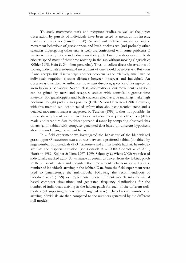
Chapter 5 – Detection of perceptual range 74
To study movement mark and recapture studies as well as the direct observation by pursuit of individuals have been tested as methods for insects, mainly for butterflies (Turchin 1998). As our work is based on studies on the movement behaviour of grasshoppers and bush crickets we (and probably other scientists investigating other taxa as well) are confronted with some problems if we try to directly follow individuals on their path. First, grasshoppers and bush crickets spend most of their time roosting in the sun without moving (Ingrisch & Köhler 1998, Hein & Gombert pers. obs.). Thus, to collect direct observations of moving individuals a substantial investment of time would be necessary. But even if one accepts this disadvantage another problem is the relatively small size of individuals requiring a short distance between observer and individual. An observer is thus likely to influence movement direction, speed or other aspects of an individuals’ behaviour. Nevertheless, information about movement behaviour can be gained by mark and recapture studies with controls in greater time intervals. For grasshoppers and bush crickets reflective tape markings make high nocturnal re-sight probabilities possible (Heller & von Helversen 1990). However, with this method we loose detailed information about consecutive steps and a detailed movement analyses suggested by Turchin (1998) is thus not possible. In this study we present an approach to extract movement parameters from (daily) mark- and recapture-data to detect perceptual range by comparing observed data on arrival in habitat with computer generated data based on different hypothesis about the underlying movement behaviour.
In a field experiment we investigated the behaviour of the blue-winged grasshopper O. caerulescens near a border between a preferred habitat (inhabited by large number of individuals of O. caerulescens) and an unsuitable habitat. In order to simulate the dispersal situation (see Conradt et al. 2000, Conradt et al. 2001, Harrison 1989, Zollner & Lima 1997, 1999, Schooley & Wiens 2003) we released individually marked adult O. caerulescens at certain distances from the habitat patch in the adjacent matrix and recorded their movement behaviour as well as the number of individuals arriving in the habitat. Data from the field experiment were used to parameterize the null-models. Following the recommendation of Goodwin et al. (1999) we implemented these different models into individual based computer simulations and generated frequency distributions for the number of individuals arriving in the habitat patch for each of the different null-models (all supposing a perceptual range of zero). The observed numbers of arriving individuals are then compared to the numbers generated by the different null-models.
Chapter 5 – Detection of perceptual range 75
5.2 MATERIALS AND METHODS
5.2.1 Field experiment
The species
Oedipoda caerulescens (Orthoptera: Acrididae: Locustinae), the blue-winged grasshopper, is a medium sized to large grasshopper species (15-28 mm, Bellmann 1993, Detzel 1998). Generally, O. caerulescens is classified as xero-thermophil. The species inhabits stony calcareous meadows with sparse vegetation, quarries and sand pits. Imagines are considered to be geophilic, inhabit open field and live on the ground. Larvae, however, are also found in dense vegetation.
Individuals usually move on the ground. If disturbed O. caerulescens typically fly a few meters (3 to 6 m) in half circles downhill. It is noticeable that individuals always land on an open place again. Both sexes fly spontaneously to locate mates. Very seldom flights of up to 100 m have been observed (Detzel 1998).
Field work
The study was conducted in August 2001 on the hillsides of Costermano (province of Verona, Northern Italy). The experiment took place on a meadow (in the following called the matrix), with very high vegetation cover (99%) and a mean vegetation height of 35 cm, close to a habitat patch. In the surrounding of Lake Garda such meadows are typical intervening habitat structures which separate patches of habitat from each other. The adjacent, elongated habitat patch was characterized by its southern exposition, strong inclination, sparse vegetation (20% vegetation cover) and consequently a lot of bare soil (80%). The suitability of this patch for O. caerulescens was indicated by the large number of individuals of O. caerulescens that were living on it. We have chosen explicitly this release situation with the non-habitat above the habitat to avoid that individuals only react on the release situation and instinctively walk uphill to compensate eventual escape flights (before capture) and to exclude visual detection of habitat.
To determine the ability of O. caerulescens to detect habitat we collected 21 males and 23 females from patches of suitable habitat at least 200 m away from the experimental area. The grasshoppers were individually marked with a coloured point code on the pronotum and numbered reflective tapes on the femur (Heller & von Helversen 1990, Samietz & Berger 1997, Kindvall 1999, Hein et al. 2003). This technique makes it easy to detect individuals at night and has been shown to lead to very high re-sight rates (Heller & von Helversen 1990, Kindvall 1999). Before and after marking individuals were kept in a cooling box to reduce potential handling trauma (Stettmer 1996).
Marked individuals were released in the matrix singly, next to a numbered wooden stick on a line forming a 90° angle with the border between habitat and meadow. The distance between consecutive release points was 1 m for the first 30

Chapter 5 – Detection of perceptual range 76
individuals and 2 m for the following 14 individuals (Figure 5.1). The maximum release distance to the habitat was thus 58 m. All individuals of O. caerulescens included in this study were captured on the day the experiment started. In the four nights following the release of individuals the meadow, the habitat, and the surrounding landscape up to 200 m away from the release points were intensively searched (7 students) for marked individuals. Daily movement distances and movement direction were recorded for each individual, first 5 h after release and then in 24 h intervals.
Re-sight rates
Re-sight rates allow an estimation of mortality risk, detection error and the quality of the marking method. In addition to the re-sights of individuals, we also recorded findings of lost reflective tape. Tape could either be lost accidentally, e.g. if it was not properly attached, or be left over by predators feeding on grasshoppers. Individuals that were not found on one day, but re-sighted on one of the following days (in the following ‘discontinuously found individuals’) were probably overlooked and allow an estimation of the detection failure during the experiment. Individuals that were never re-sighted after a certain day, were assumed to be either dead or to have left the monitored area (see also Hein et al. 2003).
Statistical analyses
Daily movement distances were analysed separately for individuals that had reached the habitat they and those still outside the habitat. Inter-group differences were tested with a Mann-Whitney U test. General directionality of individual movement paths was tested with the Rayleigh test (Zar 1984).
meadow with high vegetation preferred habitat
release points
α movement of grasshopper N
2.0 m 1.0 m
Figure 5.1: Schematic overview of the experimental setting and an exemplary movement path. Individuals were released in a perpendicular to the habitat border. Distance between release points were one meter for the first 30 individuals and two meter for the last 14 individuals. Turning angles were measured in relation to the habitat border.

Chapter 5 – Detection of perceptual range 77
We tested for the detection ability of grasshoppers by comparing the observed number of individuals in habitat with the predictions generated by different null-models. Based on 10000 simulation experiments for each null-model, we used a one-sided test of significance with a significance level α = 0.05. The null-model was thus rejected if less than 500 simulation runs predicted a number of individuals in the habitat as large as or larger than observed in the field.
5.2.2 Simulation experiments
Landscape and release situation
To generate adequate data for the null hypotheses we simulated the situation with the same dimensions as in the field (see above). Individuals were released on a straight line perpendicular to a border with preferred habitat. Distances between release points were one unit (in our case meter) for the first 30 individuals and two units for the last 14 individuals. The landscape itself was unlimited inasmuch as animals were neither reflected nor absorbed by an outer border. Any individual started its dispersal at the release point with an initial direction randomly drawn from the interval [0° .. 360°].
Model assumptions/development of null-models
The definition of our different null-models is based on the following considerations. As we strive for a conservative statement about the possibility of habitat detection, we decided to implement rather extreme assumptions in our null-models, i.e. assumptions likely to predict large numbers of individuals in the habitat even though habitat detection is not assumed. If individuals would not respond to the environment at all, they should exhibit a random movement across the landscape and arrive and stay in preferred habitat by chance over time. However, empirical studies have shown that many insect species do react to structural changes in their environment by a change in movement pattern (Baars 1979, Crist et al. 1992, Kindvall 1999, Hein et al. 2003). This is also true for the grasshopper species we studied (Hein, unpublished data and data this experiment). If individuals move randomly but with shorter movement distances inside than outside the habitat, they would stay with a higher probability in habitat than outside. However, the most extreme assumption is that individuals always stay in habitat once they have reached it, i.e. either edge permeability is zero (Zollner & Lima 1997) or movement ceases inside habitat. As this latter assumption is likely to generate the largest predicted numbers of individuals to end up in the habitat, it is implemented in all four null-models tested. In the simulations individuals always stay in the habitat patch once they have reached it.
The probability to reach habitat is further determined by (i) the number and length of steps taken, (ii) the mortality risk and (iii) the correlation between consecutive movement steps. This is taken into account in our four null-models:
Chapter 5 – Detection of perceptual range 78
In null-model 1 each time-step corresponds to one day in the field experiment. In each time step an individual moves a distance randomly drawn from the table of net displacement distances observed for the matrix, i.e. step lengths from individuals in habitat or reaching the habitat were excluded. In this null-model individuals thus take only one step per day. Initial direction and directions of all following steps are randomly drawn from the interval [0° .. 360°].
It is obvious that individuals will in fact not just take a single large step during a day. Daily net displacement will thus certainly be smaller than the actual movement path. In null-model 2 and null-model 3 we take into account that the possibility of more than one random step (of shorter step length) within a day increases the probability that an individual would arrive in habitat by chance due to the fact that a random walk covers a larger area. From our field observations we cannot directly estimate the real distance moved by the animals between two observations. However, we approximated minute-wise step lengths for this models using equation 1 from Turchin (1998), under the assumption of a completely random walk.
)(*1 2dEz
m = (5.1)
with ∑= 22 *1
)( dn
dE
m = mean step length/unit time z = number of desired steps (in our case: one step/minute, i.e. 1440 steps/ day) n = number of observations d = measured daily net displacement in non-habitat
This gives an estimated mean value of 0.57 units (meter)/minute.
Movement distances of 800 m/day implied by this value are certainly very unlikely but we nevertheless used this conservative value likely to predict a large number of individuals arriving in the habitat.
So far we have not taken into account that in the field a number of individuals is lost over time, which automatically reduces the possible number of arriving individuals. Thus, in contrast to null-model 2 (without mortality), for null-model 3 we additionally calculated dispersal mortality based on our recapture data and included a stepwise dispersal mortality of µ = 0.000138/minute. In both models initial movement direction and turning angles were randomly drawn from the uniform interval [0° .. 360°]. The direction of the actual step was thus not correlated with the previous steps.
Null-model 4 considers the influence of the degree of correlation between movement steps on the ability to reach habitat. In this null-model individuals started movement in a random direction and kept this direction until they reached suitable habitat. We realized this model by randomly drawing the initial direction
Chapter 5 – Detection of perceptual range 79
of an individual from the uniform interval [0° .. 360°] and maintaining this direction during the following steps. With a completely straight walk there exists no difference between a single step and a consecutive number of many small steps, thus in null-model 4 we used the same step length as in null-model 1.
As the field experiment was terminated after 4 days, the simulation time was T = 4 days (5760 minutes). As mentioned before each scenario was repeated 10 000 times with 44 individuals to generate a distribution for the number of individuals that arrived in the habitat after each day (T = 1,..,4 days; T = 440,..,5760 minutes).
5.3 RESULTS
5.3.1 Field experiment
Re-sight rates
Due to the marking technique it was possible to identify individuals without re-capturing them. Day to day re-sight rates always were above 70%. The proportion of individuals that were not continuously re-sighted was similar during the first two days, but decreased to zero on the third day (Figure 5.2). This indicates a constant detection error for the first two days. One possible reason for the oversight or loss of individuals during the experimental time could be that the complex structure of the meadow reduced the visibility of the reflective tape. But, if this were true the proportion of individuals that were not sighted on one day but re-sighted on a later day should have been greater. It seems more realistic to assume that individuals were either killed by predators or eventually left the study area (by flight). To determine the risk of disappearance we pooled the findings of reflective tapes and the number of individuals that were permanently lost and used this data in a logistic regression analysis with distance as explanatory variable for each observation day. On the first day (individuals were just released four hours before patrol) no significant influence of release distance could be detected (logistic regression p > 0.05). For days 2 and 3 the
1 2 3 4
day after release
0.0
0.2
0.4
0.6
0.8
1.0
frac
tion
of r
elea
sed
indi
vidu
als
Figure 5.2: Fraction of released individuals re-sighted inside (right hatched) and outside the habitat (left hatched), findings of reflective tape (black), individuals not found on this but on one of the following days (cross hatched) and permanently lost individuals (white) on each observation day.
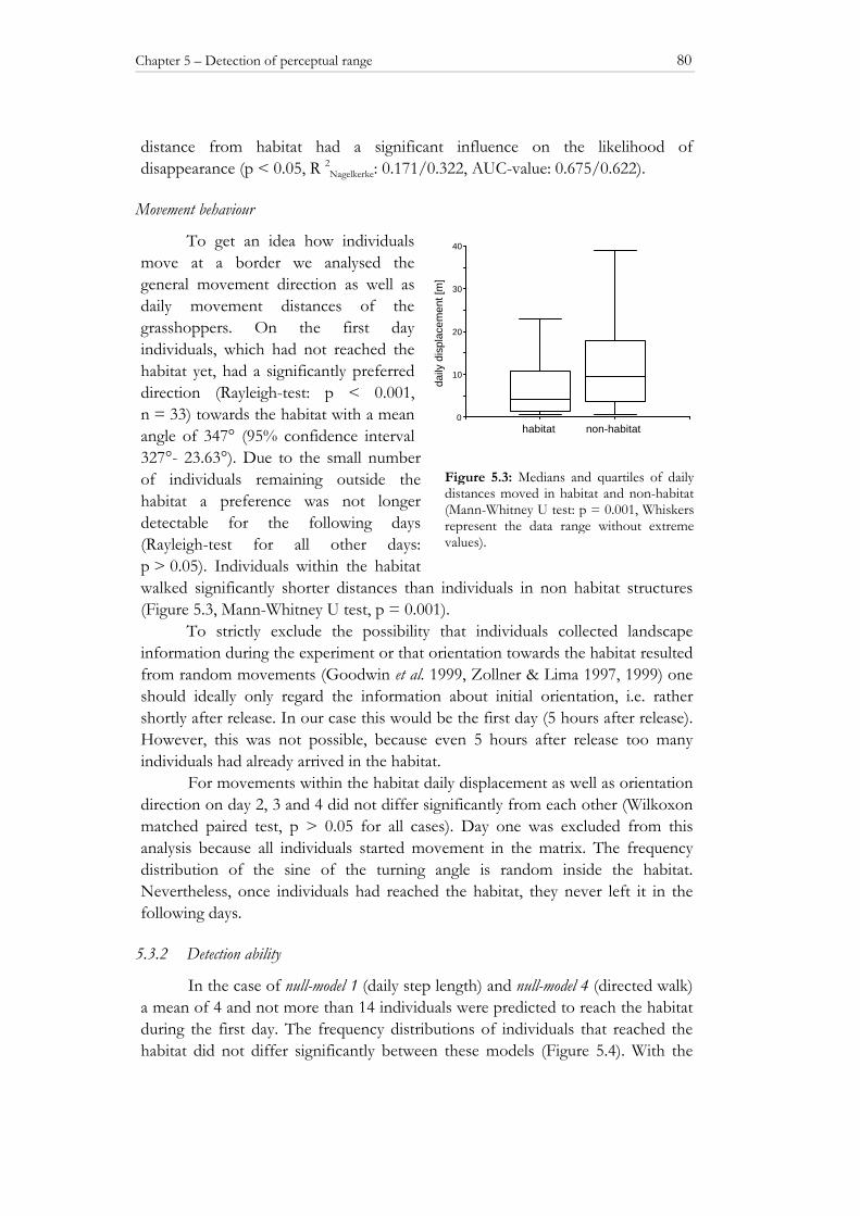
Chapter 5 – Detection of perceptual range 80
distance from habitat had a significant influence on the likelihood of disappearance (p < 0.05, R 2Nagelkerke: 0.171/0.322, AUC-value: 0.675/0.622).
Movement behaviour
To get an idea how individuals move at a border we analysed the general movement direction as well as daily movement distances of the grasshoppers. On the first day individuals, which had not reached the habitat yet, had a significantly preferred direction (Rayleigh-test: p < 0.001, n = 33) towards the habitat with a mean angle of 347° (95% confidence interval 327°- 23.63°). Due to the small number of individuals remaining outside the habitat a preference was not longer detectable for the following days (Rayleigh-test for all other days: p > 0.05). Individuals within the habitat walked significantly shorter distances than individuals in non habitat structures (Figure 5.3, Mann-Whitney U test, p = 0.001).
To strictly exclude the possibility that individuals collected landscape information during the experiment or that orientation towards the habitat resulted from random movements (Goodwin et al. 1999, Zollner & Lima 1997, 1999) one should ideally only regard the information about initial orientation, i.e. rather shortly after release. In our case this would be the first day (5 hours after release). However, this was not possible, because even 5 hours after release too many individuals had already arrived in the habitat.
For movements within the habitat daily displacement as well as orientation direction on day 2, 3 and 4 did not differ significantly from each other (Wilkoxon matched paired test, p > 0.05 for all cases). Day one was excluded from this analysis because all individuals started movement in the matrix. The frequency distribution of the sine of the turning angle is random inside the habitat. Nevertheless, once individuals had reached the habitat, they never left it in the following days.
5.3.2 Detection ability
In the case of null-model 1 (daily step length) and null-model 4 (directed walk) a mean of 4 and not more than 14 individuals were predicted to reach the habitat during the first day. The frequency distributions of individuals that reached the habitat did not differ significantly between these models (Figure 5.4). With the
habitat non-habitat0
10
20
30
40
daily
dis
plac
emen
t [m
]
Figure 5.3: Medians and quartiles of daily distances moved in habitat and non-habitat (Mann-Whitney U test: p = 0.001, Whiskers represent the data range without extreme values).
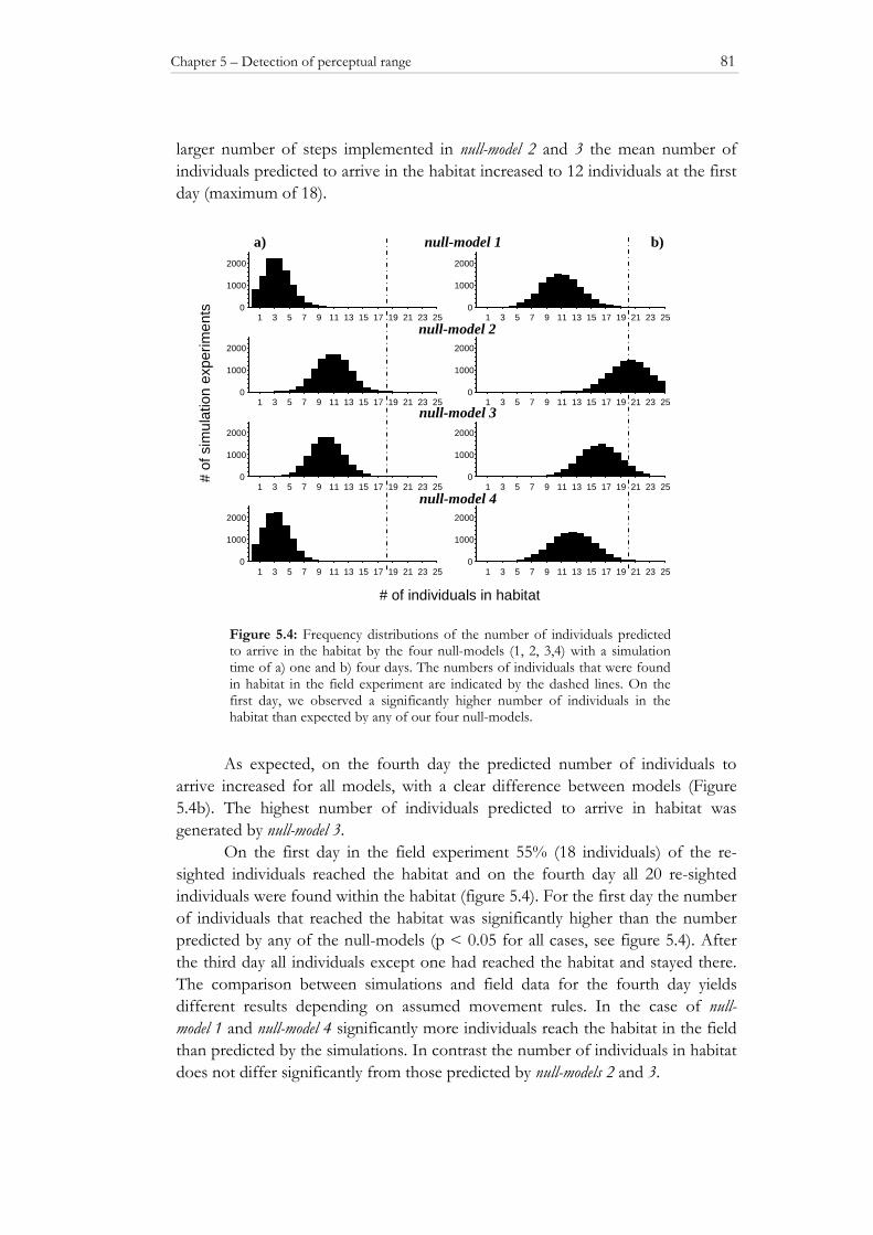
Chapter 5 – Detection of perceptual range 81
larger number of steps implemented in null-model 2 and 3 the mean number of individuals predicted to arrive in the habitat increased to 12 individuals at the first day (maximum of 18).
As expected, on the fourth day the predicted number of individuals to
arrive increased for all models, with a clear difference between models (Figure 5.4b). The highest number of individuals predicted to arrive in habitat was generated by null-model 3.
On the first day in the field experiment 55% (18 individuals) of the re-sighted individuals reached the habitat and on the fourth day all 20 re-sighted individuals were found within the habitat (figure 5.4). For the first day the number of individuals that reached the habitat was significantly higher than the number predicted by any of the null-models (p < 0.05 for all cases, see figure 5.4). After the third day all individuals except one had reached the habitat and stayed there. The comparison between simulations and field data for the fourth day yields different results depending on assumed movement rules. In the case of null-model 1 and null-model 4 significantly more individuals reach the habitat in the field than predicted by the simulations. In contrast the number of individuals in habitat does not differ significantly from those predicted by null-models 2 and 3.
Figure 5.4: Frequency distributions of the number of individuals predicted to arrive in the habitat by the four null-models (1, 2, 3,4) with a simulation time of a) one and b) four days. The numbers of individuals that were found in habitat in the field experiment are indicated by the dashed lines. On the first day, we observed a significantly higher number of individuals in the habitat than expected by any of our four null-models.
1 3 5 7 9 11 13 15 17 19 21 23 250
1000
2000
1 3 5 7 9 11 13 15 17 19 21 23 250
1000
2000
1 3 5 7 9 11 13 15 17 19 21 23 250
1000
2000
1 3 5 7 9 11 13 15 17 19 21 23 250
1000
2000
1 3 5 7 9 11 13 15 17 19 21 23 250
1000
2000
1 3 5 7 9 11 13 15 17 19 21 23 250
1000
2000
1 3 5 7 9 11 13 15 17 19 21 23 250
1000
2000
1 3 5 7 9 11 13 15 17 19 21 23 250
1000
2000
null-model 2
null-model 3
null-model 4
a) null-model 1 b)
# of individuals in habitat
# of
sim
ulat
ion
expe
rimen
ts
Chapter 5 – Detection of perceptual range 82
5.4 DISCUSSION
5.4.1 Re-sight rates
In comparison to other studies day to day re-sight rates above 70 % can be classified as satisfactory for non-habitat structures (see Ingrisch & Köhler 1998, Kindvall 1999, Hein et al. 2003). The increase in the probability to disappear with increasing distance to habitat may result from the fact that individuals further away from the border stay longer in the matrix than individuals close to the border and thus are longer exposed to a higher mortality risk. This is likely to be the case because outside their habitat individuals are not well camouflaged against predators. Additionally, for the case of O. caerulescens other and more predators maybe found on the meadow than in the habitat of the species. On the other hand one cannot exclude that some individuals performed long distance dispersal and thus were not re-sighted.
5.4.2 Simulation experiments and detection ability
After one day 18 out of the 44 grasshoppers released in the matrix were already found in the habitat, on the fourth day the number raised to 20 individuals. Clearly, individuals seem to react to the border since all individuals stayed within the habitat after they had reached it. Consequently our assumption of an edge permeability of zero seems to be warranted. All in all, on the first day more individuals than predicted by any of our four null-models reached the preferred habitat. This is especially noticeable as for the first day simulations run for 24 h, whereas in the field experiment individuals only had 5 hours for orientation and movement towards the habitat.
The simulation experiments show that even without the ability to detect habitat from a distance, altered rules for individuals behaviour can significantly increase the fraction of individuals predicted to reach the habitat. Obviously, an increase in the temporal resolution, i.e. number of steps (null-model 2, null-model 3) increases the fraction of individuals predicted to arrive in the habitat patch. Nevertheless, for the first day we thus believe that in our field experiment individuals did not move randomly but perceived their habitat from a certain distance. However, we cannot completely rule out alternative explanations for the difference between observed and predicted numbers of grasshoppers arriving in habitat. For example, a systematic search for habitat following the pathway of an Archimedian spiral or any other non-random movement might lead to a sooner detection of habitat than predicted by our models. But we have no indication why we should assume such a systematic search by our species. Preliminary movement experiments with O. caerulescens inside different types of habitat and non-habitat structures did not show significantly preferred movement directions (Hein unpublished data).

Chapter 5 – Detection of perceptual range 83
In general, one should give most weight to the results for the first day as with increasing time other mechanisms like the gathering of information about the surrounding landscape, species condition or an increased mortality risk may change and influence the results. Principally, model predictions should come closer to one another over longer periods of time.
5.4.3 Movement behaviour and perceptual range
Given that a detection of habitat from a distance is principally proven, it becomes interesting to know from which distance individuals are exactly capable to detect habitat. At the moment an individual recognizes habitat in a distance it should alter its behaviour (otherwise we would not have cues that it detected the habitat, Zollner & Lima 1999). For example, individual movement paths should become more directed and/or faster. Generally, the analyses of such changes in behaviour are ideally based on direct, small scale observations of individuals. However, a combination between both direct pursuit and simulation experiments like those presented here are a ‘second-best’ solution in cases were permanent pursuit cannot be conducted for technical or financial reasons. Unfortunately, in our case such an analyses was not possible as even after 5 h of release too many individuals had reached the habitat already. For further studies we would recommend a combination of both, direct observations of the initial orientation behaviour of single individuals once shortly after release and mark-recapture studies with longer time intervals. This would allow for a thorough analysis of initial orientation as well as arrival data.
An effect of distance on patch detection was found by other authors, with detection distances ranging from very short distances of < 0.3 m for skippers (Capman et al., 1990) and < 2 m for flea beetles (Kareiva 1985) up to 10-22 m from the habitat boundary for butterflies (Schultz & Crone 2001). It is hard to know how the individuals actually detected the habitat. We tend to exclude attraction by conspecific songs because O. caerulescens only produces scratches of low-intensity. Some insects can orientate very well olfactory (Schooley & Wiens 2003), but little is known about the olfactory abilities of grasshoppers. In any case, we could not find a habitat-specific plant which might serve as an olfactory cue. In our view the most likely way of orientation is the visual detection of open ground. This could be achieved by short orientation flights. Although we did not observe such flights in the field we cannot exclude them. Another possible way of orientation would be the recognition of the heat radiated by infra-red radiation of the open areas, which should be much higher than for the dense vegetation of the meadow.
If individuals can differentiate between their habitat and non–habitats their probability to stay inside the habitat at a habitat boundary should increase. In our study individuals that had reached the habitat never left it again, although the elongated structure of the habitat should increase boundary encounters. Adding
Chapter 5 – Detection of perceptual range 84
such edge-mediated behaviour to simulation studies leads to an increased residence time (Schultz & Crone 2001). This has strong influence on population parameters such as emigration rate and therefore influences long-term survival of metapopulations (Schultz & Crone 2001).
On the other hand, perception of habitat increases colonization probability due to reduced search time and (likely) reduced dispersal mortality (Gaines & McClenaghan 1980, Doak et al. 1992, Hanski & Zhang 1993). Including a perceptual range into metapopulation models would thus alter immigration rates, and consequently influence measures of habitat connectivity due to the increase in the ‘effective patch area’ (Meriam 1991, Schooley & Wiens 2003). This would result in shorter effective distances between patches (Hanski 1994a, b) but also in an increased ‘shadow effect’ of patches exerted on other patches laying behind them (cf. Hein et al. in press). In fact, a very large perceptual range may diminish the importance of factors such as the spatial arrangement of habitat patches on population dynamics. Based on our results we support the notion that landscapes should be described with respect to the behavioural and physiological abilities of the animals under study (Meriam 1991, Johnson et al. 1992, Wiens et al. 1993, With 1994, Hein et al. 2003).
Chapter 6
Patch density, movement pattern, and realised dispersal distances in a patch-matrix
landscape – a simulation study
with Brenda Pfenning, Thomas Hovestadt and Hans-Joachim Poethke
ECOLOGICAL MODELLING (IN PRESS)
Abstract. In metapopulation models it is common practice to use species specific dispersal distances to predict the exchange of individuals between habitat patches. The influence of patch distribution on the reachability of a habitat patch is usually ignored. In a patch-matrix simulation we investigated the effect of patch number, movement pattern and dispersal mortality on realized animal dispersal distances.
In our spatially-explicit, individual-based simulations we demonstrate that: 1. with increasing number of patches the number of immigrants into patches further away from the release point decreases in all scenarios (‘shadow effect’) 2. this effect is strongest for a random movement 3. for rather uncorrelated walks a proper adjustment of mean dispersal distance in the negative exponential model can account for the effect of patch density on realized dispersal distances 4. with a more directed walk this is not possible as the distribution of moving animals in the matrix becomes highly heterogeneous. This is due to the narrow but far reaching shadow patches exert on other patches further away from the release point.

Chapter 6 – Realised dispersal distances in patch-matrix landscape 87
6.1 INTRODUCTION
Long-term persistence and stability of (meta-) populations within fragmented landscapes crucially depends on recolonisation between habitat patches (Gustafson & Gardner 1996). Colonization probability is implicitly limited by inter-patch distance and dispersal ability of the species in question. Consequently, dispersal is assumed to be one key process responsible for metapopulation persistence (Hanski 1994, Hanski & Thomas 1994, Hill et al. 1996; Moilanen & Hanski 1998, Moilanen & Nieminen 2002). It determines the long-term survival of metapopulations due to demographic as well as genetic effects (Levins 1969, den Boer 1981, Taylor 1990, Cohen & Levin 1991, McCauley 1995, Cresswell 1997, With et al. 1999, Poethke et al. 2003). Additionally, dispersal is an important factor determining local extinctions (Poethke et al. 1996a, b).
In his widely recognised incidence function model, Hanski (1994) assumes that inter-patch dispersal depends on the distance between patches and the general dispersal capabilities of the species under study. The model assumes that the exchange of individuals between patches can readily be described by a negative exponential distribution. This approach is easy to handle, makes clear predictions, is theoretically well based (MacArthur & Wilson 1967, Pulliam 1988) and thus often used in modelling species dispersal across landscapes (Hanski & Thomas 1994, Hanski & Gilpin 1997, With & King 1999a, b).
Recently, this simplifying approach has been criticised for a variety of reasons. First, dispersal will be affected by the quality of the matrix (Gustafson & Gardner 1996, Moilanen & Hanski 1998, Thomas et al. 2001, Wiegand et al. 1999, Wiens 2001) in which dispersal takes place. Second, it also may be affected by the distribution of suitable habitat patches in the landscape (Gustafson & Gardner 1996, Zollner & Lima 1999b, King & With 2002). If these objections are founded, we should find dispersal parameters to depend not only on a species traits but also on the specific characteristics of a given landscape. Therefore it is important to investigate the effects of landscape structure on the distribution of dispersal distances.
One possibility to obtain dispersal distance distributions for the prediction of colonization probabilities at the landscape level is to fit dispersal kernels to the empirically observed distance distributions (e.g. Paradis et al. 2002). However, successful patch to patch dispersal, which is usually long-distance dispersal, is hard to investigate, as recapture rates are generally low and individuals are hard to follow (Gaines & Bertness 1993, see also Zollner & Lima 1999a). Consequently, only a few studies on dispersal at landscape level, mostly on butterfly dispersal, are available (e.g. Harrison 1989, Baguette & Nève 1994, Hanski et al. 1994, Hill et al. 1996, Kuussaari et al. 1996, Nève et al. 1996a,b, Sutcliffe et al. 1997, Brommer & Fred 1999). On the other hand, if data are available and dispersal kernels can be

Chapter 6 – Realised dispersal distances in patch-matrix landscape 88
fitted, this does not allow to differentiate between the effect of variation in dispersal behaviour of the species, the influence of the matrix, or the impact of number of patches on realized dispersal distances.
A second approach to determine colonization probabilities at the landscape level is based on information about the habitat specific movement patterns of a species. In simulation studies this pattern can be extrapolated to dispersal at the landscape scale (Dunning et al. 1995, South et al. 2002). Data are derived from empirical studies which focus on small scale movement of animals in habitats of different structure and resistance (Wiens & Milne 1989, Kareiva 1990, Crist et al. 1992, Haefner & Crist 1994, With & Crist 1995, Wiens et al. 1997) or suitability (Wiens et al. 1997, Schultz 1998, Kindvall 1999, Wiens 2001, Hein et al. 2003) as well as on the behaviour at borders between different types of habitat (Conradt et al. 2000, Schultz & Crone 2001).
In this paper we use such a mechanistic simulation study to investigate the relevance of the number of habitat patches, movement pattern and dispersal mortality on the distribution of realized dispersal distances. We model dispersing individuals which leave their home patch to search for new habitat patches in a heterogeneous landscape consisting of a hostile matrix and a variable number of suitable habitat patches. Although our simulation is motivated by our fieldwork with bush crickets in patchy semiarid grasslands, our results should be qualitatively applicable to other species as well.
6.2 METHODS
We simulated the movement of dispersing animals in a landscape with patches of suitable habitat distributed in an unsuitable matrix. Because we focus on reachability of patches and realized dispersal distances of individuals, there is no need to consider the size or dynamics of local populations or of a metapopulation at large. Midpoints of circular patches of suitable habitat of equal size (one hectare (1 * 104 m2), r = 56.4 m) were distributed inside a circular arena (R = 1000 m; 3.14 * 106 m2) around the central ‘release point’. The edge of this arena was implemented as a neither reflecting nor absorbing border. Patches were distributed at random within this arena, but were eventually relocated to fulfil two conditions. (i) The minimum distance of the centre of a patch from the release point had to be larger than 2 r. (ii). Patches were not allowed to overlap, i.e. the distance between the centres of any two patches had to be larger than 2 r. In this respect, our model is similar to that of Zollner and Lima (1999b).
In the simulations, any individual started its dispersal at the central release point in the matrix with an initial direction randomly drawn from the uniform interval [0° .. <360°]. At each time-step an individual moved a certain distance
Chapter 6 – Realised dispersal distances in patch-matrix landscape 89
drawn from a table of daily step lengths (n=159) empirically derived for the movement of bush crickets Platycleis albopunctata in unsuitable habitat (Hein et al. 2003). These data were approximately negative exponentially distributed with a mean dispersal distance (D) of 8.62 m, i.e. less than 1/10 of a patch’s diameter. To cover the range of movement patterns observed for different insect species we implemented three different movement rules to alter the direction of an individual:
‘Cricket walk’: A movement pattern with turning angles drawn from an empirically derived distribution for Platycleis albopunctata. This movement pattern results in a correlated random walk as turning angles (measured against the direction of the previous step) were distributed nearly uniformly in the interval [-172° .. 170°] (for a similar approach see Kindvall 1999).
‘Directed walk’: A directed (linear) walk, i.e. animals exactly maintained the direction randomly selected at the beginning of their path. Examples of (fairly) directional movements have been observed for individuals that detect their habitat patch from a certain distance (Conradt et al. 2000, Schultz & Crone 2001) or that move in unsuitable habitat (e.g. beetles, Baars 1979, Crist et al. 1992, Roslin 2000; crickets, Kindvall 1999; hedgehogs, Doncaster et al. 2001).
‘Random walk’: A completely (uncorrelated) random walk, i.e. for each step the direction was randomly taken from the uniform interval [-180°..180]. The direction of the actual step was thus not correlated with that of any previous step. Consequently, this movement pattern should become similar to that of a Brownian diffusion process. Empirical examples for a (nearly) random walk can be found for individuals that move in suitable habitat (Crist et al. 1992, Kindvall 1999, Schultz 1998).
In our simulations, the movement of an animal was terminated as soon as one of the following events occurred: (i) the animal arrived in a patch of habitat, (ii) the animal died (with stepwise dispersal mortality m, see below), (iii) the maximum simulation time was reached. Maximum simulation time T = 300 was chosen to allow mean net-displacement in a landscape without habitat patches to surpass R.
To investigate the effect of patch number, movement pattern, and dispersal mortality on the distance distribution of animals arriving in a habitat patch, we tested all combinations of the following parameter values. (i) Patch number (P) with P = 1, 8, 16, 32, or 64. (ii) The three movement patterns described above, i.e. ‘cricket walk’, ‘directed walk’ and ‘random walk’. (iii) Step-wise dispersal mortality m set to m = 0.01 or 0.02. Implicitly, we thus assume mortality to be a purely random process independent of the previous travel history. The resulting mean survival times for these two values, i.e. 100 or 50 time steps (days), fall into a realistic range as the activity period of bush crickets varies between 60 and 150 days (see Detzel 1998, Kindvall 1999). Additionally, we included simulations with no dispersal mortality (m = 0.0) – a highly unlikely situation in nature – to study the pure interaction effect of patch number and movement pattern. For each parameter combination we ran simulations on 1000 different random landscape

Chapter 6 – Realised dispersal distances in patch-matrix landscape 90
with 1000 individuals each. In total we thus produced movement paths for 1 * 106 simulated individuals.
Over the course of a simulation run we counted the number of individuals arriving in each patch and – at its end – estimated the realized mean dispersal distance (D), i.e. the mean travel distance for all individuals which arrived in a patch. For analysis and presentation of the data, patches were pooled into distance classes and mean values of arriving individuals were estimated for all patches within a given distance class.
To visualize the effects of movement pattern and high patch density, we ran one additional simulation for the random walk as well as the directed walk. In each scenario we simulated 10 000 individuals over 1000 time steps in a landscape with 64 patches (r = 2 m). The landscape was divided into a regular grid of 40 000 (200 x 200; R = 100 m) cells of 1 m x 1 m. Step length was distributed uniformly in the interval [0..1]. We counted how many individuals were sighted in each cell throughout the whole simulation time. The spatial distribution of these counts represents the accumulated density distribution for the likelihood to observe a moving individual that started at the ‘release point’ in that area of the matrix and gives an intuitive idea about the reachability of different regions in the artificial landscape. Clearly, a habitat patch is more likely to ‘collect’ many immigrants if surrounded by matrix with a high density distribution than if surrounded by matrix with a low density distribution.
Chapter 6 – Realised dispersal distances in patch-matrix landscape 91
6.3 RESULTS
6.3.1 Single-patch scenario.
First, we tested the effect of movement pattern and dispersal mortality on the distance-dependent reachability of a solitary patch. Expectedly, more individuals arrive in patches in scenarios without than with mortality (Figure 6.3). The single-patch scenario corresponds to the isolation-by-distance situation with inter-patch dispersal independent of the landscape structure (cf. Hanski 1994, Kitching 1971). Not surprisingly, the probability to reach a patch decreases with increasing distance between the patch and the release point for all tested parameters (Figure 6.1).
Though the commonly used negative exponential fit produces high coefficients of determination for a ‘directed walk’, this distribution does not represent the data adequately. It overestimates short distance dispersal and underestimates the tail of the distribution (cf. Dobzhansky & Wright 1943, Harrison 1989, Hill et al. 1996) which is the most interesting part regarding dispersal distances and colonization probabilities. For an exactly straight walk, the expected distribution for the distance dependent probability of arrival (P(d)) should follow an arcsine-function.
P(d) = 1/π * arcsine(2r/d) (6.1) with d = distance between release point and centre of patch and 2r = diameter of patch.
For d >> r this relationship can be approximated by a simple power
function, i.e.
P(d) ≈ 1/π * 2r/d (6.2)
Consistently, for the directed movement pattern the relationship is better described by a power distribution. For the random walk, the relationship between dispersal distance and the probability to reach a patch can accurately be described by a negative exponential distribution (cf. Kitching 1971, Figure 6.1b). Implementation of the empirical distribution (‘cricket walk’) for turning angles and step length results in a distribution also consistent with the negative exponential model.
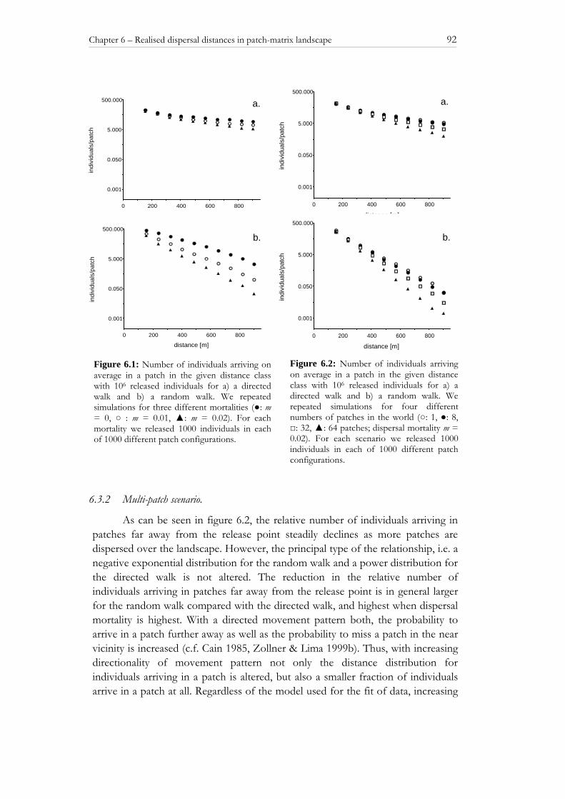
Chapter 6 – Realised dispersal distances in patch-matrix landscape 92
6.3.2 Multi-patch scenario.
As can be seen in figure 6.2, the relative number of individuals arriving in patches far away from the release point steadily declines as more patches are dispersed over the landscape. However, the principal type of the relationship, i.e. a negative exponential distribution for the random walk and a power distribution for the directed walk is not altered. The reduction in the relative number of individuals arriving in patches far away from the release point is in general larger for the random walk compared with the directed walk, and highest when dispersal mortality is highest. With a directed movement pattern both, the probability to arrive in a patch further away as well as the probability to miss a patch in the near vicinity is increased (c.f. Cain 1985, Zollner & Lima 1999b). Thus, with increasing directionality of movement pattern not only the distance distribution for individuals arriving in a patch is altered, but also a smaller fraction of individuals arrive in a patch at all. Regardless of the model used for the fit of data, increasing
Figure 6.2: Number of individuals arriving on average in a patch in the given distance class with 106 released individuals for a) a directed walk and b) a random walk. We repeated simulations for four different numbers of patches in the world (○: 1, ●: 8, □: 32, ▲: 64 patches; dispersal mortality m = 0.02). For each scenario we released 1000 individuals in each of 1000 different patch configurations.
0 200 400 600 800
distance [m]
0.001
0.050
5.000
500.000
indi
vidu
als/
patc
h
0 200 400 600 800
distance [m]
0.001
0.050
5.000
500.000
indi
vidu
als/
patc
h
a.
b.
Figure 6.1: Number of individuals arriving on average in a patch in the given distance class with 106 released individuals for a) a directed walk and b) a random walk. We repeated simulations for three different mortalities (●: m = 0, ○ : m = 0.01, ▲: m = 0.02). For each mortality we released 1000 individuals in each of 1000 different patch configurations.
0 200 400 600 800
distance [m]
0.001
0.050
5.000
500.000
indi
vidu
als/
patc
h
0 200 400 600 800
distance [m]
0.001
0.050
5.000
500.000
indi
vidu
als/
patc
h
a.
b.
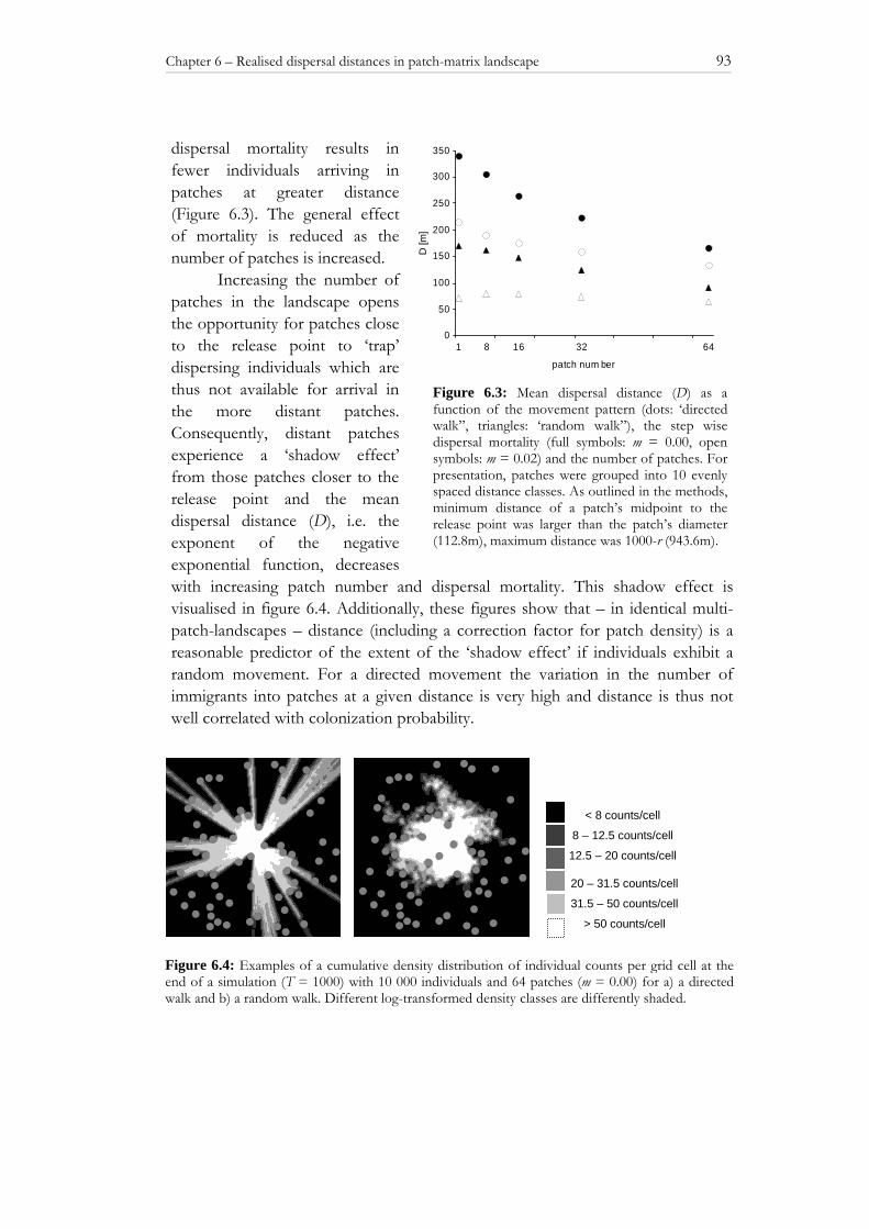
Chapter 6 – Realised dispersal distances in patch-matrix landscape 93
dispersal mortality results in fewer individuals arriving in patches at greater distance (Figure 6.3). The general effect of mortality is reduced as the number of patches is increased.
Increasing the number of patches in the landscape opens the opportunity for patches close to the release point to ‘trap’ dispersing individuals which are thus not available for arrival in the more distant patches. Consequently, distant patches experience a ‘shadow effect’ from those patches closer to the release point and the mean dispersal distance (D), i.e. the exponent of the negative exponential function, decreases with increasing patch number and dispersal mortality. This shadow effect is visualised in figure 6.4. Additionally, these figures show that – in identical multi-patch-landscapes – distance (including a correction factor for patch density) is a reasonable predictor of the extent of the ‘shadow effect’ if individuals exhibit a random movement. For a directed movement the variation in the number of immigrants into patches at a given distance is very high and distance is thus not well correlated with colonization probability.
a.
< 8 counts/cell
8 – 12.5 counts/cell
12.5 – 20 counts/cell
20 – 31.5 counts/cell
31.5 – 50 counts/cell
> 50 counts/cell
Figure 6.4: Examples of a cumulative density distribution of individual counts per grid cell at the end of a simulation (T = 1000) with 10 000 individuals and 64 patches (m = 0.00) for a) a directed walk and b) a random walk. Different log-transformed density classes are differently shaded.
1 8 16 32 64
patch num ber
0
50
100
150
200
250
300
350
D [m
]
Figure 6.3: Mean dispersal distance (D) as a function of the movement pattern (dots: ‘directed walk”, triangles: ‘random walk”), the step wise dispersal mortality (full symbols: m = 0.00, open symbols: m = 0.02) and the number of patches. For presentation, patches were grouped into 10 evenly spaced distance classes. As outlined in the methods, minimum distance of a patch’s midpoint to the release point was larger than the patch’s diameter (112.8m), maximum distance was 1000-r (943.6m).

Chapter 6 – Realised dispersal distances in patch-matrix landscape 94
6.4 DISCUSSION
In most metapopulation models a negative exponential relationship is assumed to describe the distribution of dispersal distances (e.g. Hanski 1994, Nieminen 1996). This adequately represents the movement behaviour of the majority of species studied empirically. However, in agreement with recent empirical (Wiens et al. 1997, Baguette et al. 2000) and theoretical studies (Portnoy & Willson 1993, Clark 1998, Clark et al. 1998, 1999, Higgins & Richardson 1999, Hovestadt et al. 2001) our own simulations show, that this assumption may not always be met. It depends critically on the kind of movement pattern and will almost surely be violated whenever animal movement becomes very directed. In such cases an arcsine-function (or the power function) will more adequately describe the distribution of dispersal distances (cf. Portnoy & Willson 1993, Hill et al. 1996, Kot et al. 1996 and references therein, Turchin 1998).
Principally, the path taken by an individual (without mortality) and the mortality risk can be seen as two independent random factors influencing the final fate of a moving individual, i.e. whether it will arrive in a patch at all (in the limited time of the experiment) and if so, which patch it will be. For the interpretation of the influence of mortality on realized dispersal distances, we thus can also consider the time it took an individual to arrive in the target patch (for the scenario without mortality) and then ask in behind, whether it would have arrived if mortality had occurred. Clearly, an individual which took longer would have had a lower chance of arrival than an individual which arrived soon. Evidently, it will on average take longer to arrive in a distant patch than in a patch close to the release point – and this especially holds for random walk where net-displacement only increases in proportion to the square root of travel time (Turchin 1998).
These basic facts allow to explain the two patterns observed with the introduction of dispersal mortality. (i) The relative reduction in mean dispersal distance is larger for the random walk. This is due to the fact that the individuals arriving in distant patches have used longer time spans than in the scenario with a directed walk and will thus suffer more strongly from dispersal mortality. (ii) The general effect of mortality is reduced as the number of patches is increased. This is can be explained by the fact that the average travel time needed to arrive in a patch declines as patch density is increased. Thus, a larger fraction of individuals will have the chance to arrive in a patch before they eventually die.
In addition to the influence of movement pattern and dispersal mortality on the resulting species specific dispersal distance distributions, the results of our simulation experiments clearly demonstrate, that landscape structure (in our case the number and distribution of habitat patches) can have a significant effect on the exchange of individuals between habitat patches. Besides variable matrix structure (see Wiens et al. 1997) and the changing mortality risk during dispersal (Pulliam et al. 1992, Wiegand et al. 1999) we can thus add the spatial distribution of patches to
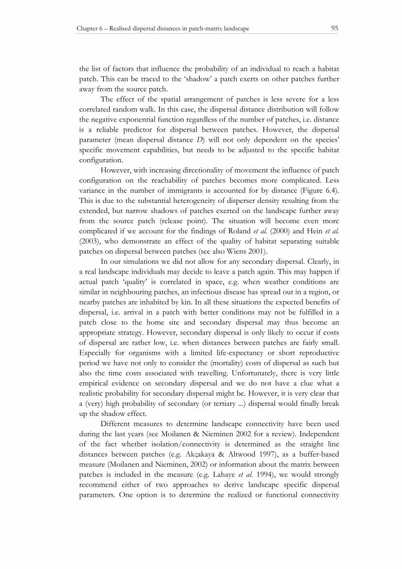
Chapter 6 – Realised dispersal distances in patch-matrix landscape 95
the list of factors that influence the probability of an individual to reach a habitat patch. This can be traced to the ‘shadow’ a patch exerts on other patches further away from the source patch.
The effect of the spatial arrangement of patches is less severe for a less correlated random walk. In this case, the dispersal distance distribution will follow the negative exponential function regardless of the number of patches, i.e. distance is a reliable predictor for dispersal between patches. However, the dispersal parameter (mean dispersal distance D) will not only dependent on the species’ specific movement capabilities, but needs to be adjusted to the specific habitat configuration.
However, with increasing directionality of movement the influence of patch configuration on the reachability of patches becomes more complicated. Less variance in the number of immigrants is accounted for by distance (Figure 6.4). This is due to the substantial heterogeneity of disperser density resulting from the extended, but narrow shadows of patches exerted on the landscape further away from the source patch (release point). The situation will become even more complicated if we account for the findings of Roland et al. (2000) and Hein et al. (2003), who demonstrate an effect of the quality of habitat separating suitable patches on dispersal between patches (see also Wiens 2001).
In our simulations we did not allow for any secondary dispersal. Clearly, in a real landscape individuals may decide to leave a patch again. This may happen if actual patch ‘quality’ is correlated in space, e.g. when weather conditions are similar in neighbouring patches, an infectious disease has spread out in a region, or nearby patches are inhabited by kin. In all these situations the expected benefits of dispersal, i.e. arrival in a patch with better conditions may not be fulfilled in a patch close to the home site and secondary dispersal may thus become an appropriate strategy. However, secondary dispersal is only likely to occur if costs of dispersal are rather low, i.e. when distances between patches are fairly small. Especially for organisms with a limited life-expectancy or short reproductive period we have not only to consider the (mortality) costs of dispersal as such but also the time costs associated with travelling. Unfortunately, there is very little empirical evidence on secondary dispersal and we do not have a clue what a realistic probability for secondary dispersal might be. However, it is very clear that a (very) high probability of secondary (or tertiary ...) dispersal would finally break up the shadow effect.
Different measures to determine landscape connectivity have been used during the last years (see Moilanen & Nieminen 2002 for a review). Independent of the fact whether isolation/connectivity is determined as the straight line distances between patches (e.g. Akςakaya & Altwood 1997), as a buffer-based measure (Moilanen and Nieminen, 2002) or information about the matrix between patches is included in the measure (e.g. Lahaye et al. 1994), we would strongly recommend either of two approaches to derive landscape specific dispersal parameters. One option is to determine the realized or functional connectivity

Chapter 6 – Realised dispersal distances in patch-matrix landscape 96
(sensu Wiens et al. 1997, With et al. 1999) by modelling dispersal behaviour within a landscape context to get landscape specific matrices of exchange between patches (cf. South 1999, Pfenning et al. in revision). This requires proper knowledge of the effect of all relevant factors, i.e. the intervening habitat as well as the arrangement of suitable habitat and individual movement behaviour. This approach may be specifically indicated, if we strive for the design of population models to develop optimal conservation strategies (see South et al. 2002). In such a case, a precise prediction of extinction- and survival-probabilities of animal populations is of essential importance. As an alternative, at least under some conditions simple correction factors accounting for patch density and inter-patch distance, may be applied to adjust estimates of colonization probability to any specific landscape (cf. Heinz et al. submitted).

Summary 97
Summary
The progressive exploitation of landscapes by man increases fragmentation of valuable areas with high biodiversity (e.g. mesoxerophytic grasslands). Consequently, many populations nowadays exist as metapopulations, i.e. ensembles of small local populations not capable of long-term survival without interactions with neighbouring populations (Ehrlich et al. 1980, Hanski 1994a, b, Thomas & Hanski 1997). In such cases, the balance between extinction and colonisation of (vacant) patches determines the regional survival of species (Levins 1969, Hanski 1994, Hanski & Thomas 1994, Hill et al. 1996). To determine long term survival of species and to assess the impact of different management regimes proper knowledge of species habitat requirements as well as information on their dispersal behaviour is needed. The aim of this thesis was to develop methods and measures for the identification of suitable areas for grasshoppers and bush crickets, as well as to quantify the reachability of single patches by individuals.
The first part of my work (Chapters 2 & 3) focuses on the quantification of habitat suitability for grasshoppers and bush crickets. A good habitat patch is characterised by high habitat capacity, i.e. its area as well as quality (Thomas et al. 2001). In my work I concentrated on the determination of habitat quality for two bush cricket and one grasshopper species on three spatial scales. Based on presence/absence data, I developed statistical habitat suitability models using logistic regression analyses. The resulting models are evaluated and validated in space and time. It turned out that habitat selection of the three species mainly took place on an intermediate spatial scale, as only parameters measured directly at the experimental plot or close to it significantly increase the power of the final models. The relevant scale falls into the same range as the species’ mean dispersal distances. Besides the rather coarse grained factor ‘type of habitat’ structural factors like vegetation height, as well as abiotic factors like exposition or solar radiation are correlated with the occurrence of the species.
The model of S. lineatus, including the parameters ‘type of biotope’ and ‘vegetation height’ was most successful in predicting the occurrences of the bush cricket species. To further test whether the occurrence of species of different insect groups can be predicted with a common model, I tested the usefulness of the orthoptera models for the prediction of butterflies in the same region and vice versa. While transferability of the orthoptera models was poor, the model of the moth Z. carniolica performed quite successful. It included the proportion of suitable habitat (fringes, mesoxerophytic grasslands, extensively managed meadows) as well as the occurrence of the two sucking plants C. jacea and S. columbaria as relevant factors. Z. carniolica is classified as stenoecious and thus represents other species typically found on fringes and mesoxerophytic grasslands. The high mobility of Z. carniolica simultaneously guarantees the
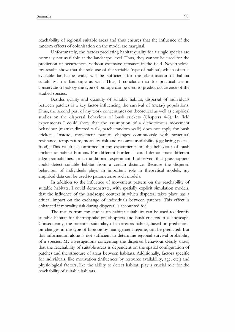
Summary 98
reachability of regional suitable areas and thus ensures that the influence of the random effects of colonisation on the model are marginal.
Unfortunately, the factors predicting habitat quality for a single species are normally not available at the landscape level. Thus, they cannot be used for the prediction of occurrences, without extensive censuses in the field. Nevertheless, my results show that the sole use of the variable ‘type of habitat’, which often is available landscape wide, will be sufficient for the classification of habitat suitability in a landscape as well. Thus, I conclude that for practical use in conservation biology the type of biotope can be used to predict occurrence of the studied species.
Besides quality and quantity of suitable habitat, dispersal of individuals between patches is a key factor influencing the survival of (meta-) populations. Thus, the second part of my work concentrates on theoretical as well as empirical studies on the dispersal behaviour of bush crickets (Chapters 4-6). In field experiments I could show that the assumption of a dichotomous movement behaviour (matrix: directed walk, patch: random walk) does not apply for bush crickets. Instead, movement pattern changes continuously with structural resistance, temperature, mortality risk and resource availability (egg laying places, food). This result is confirmed in my experiments on the behaviour of bush crickets at habitat borders. For different borders I could demonstrate different edge permabilities. In an additional experiment I observed that grasshoppers could detect suitable habitat from a certain distance. Because the dispersal behaviour of individuals plays an important role in theoretical models, my empirical data can be used to parameterise such models.
In addition to the influence of movement pattern on the reachability of suitable habitats, I could demonstrate, with spatially explicit simulation models, that the influence of the landscape context in which dispersal takes place has a critical impact on the exchange of individuals between patches. This effect is enhanced if mortality risk during dispersal is accounted for.
The results from my studies on habitat suitability can be used to identify suitable habitat for thermophilic grasshoppers and bush crickets in a landscape. Consequently, the potential suitability of an area as habitat, based on predictions on changes in the type of biotope by management regime, can be predicted. But this information alone is not sufficient to determine regional survival probability of a species. My investigations concerning the dispersal behaviour clearly show, that the reachability of suitable areas is dependent on the spatial configuration of patches and the structure of areas between habitats. Additionally, factors specific for individuals, like motivation (influences by resource availability, age, etc.) and physiological factors, like the ability to detect habitat, play a crucial role for the reachability of suitable habitats.
Zusammenfassung 99
Zusammenfassung
Die zunehmende anthropogene Nutzung von Landschaften führt zu einer steigenden Fragmentierung schützenswerter Flächen (wie z.B. Halbtrockenrasen) mit hoher Artendiversität. Damit verbunden ist gleichzeitig eine Zerschneidung von großen, zusammenhängenden Populationen in sogenannte Metapopulationen, d.h. in Verbände von kleinen lokalen Populationen, die jeweils ohne den Austausch mit anderen Populationen langfristig nicht überleben könnten (Ehrlich et al. 1980, Hanski 1994, Thomas & Hanski 1997). In solchen Fällen bestimmt das Gleichgewicht zwischen Aussterben und (Wieder-) Besiedlung von Habitaten die regionale Überlebenswahrscheinlichkeit von Arten (Levins 1969, Hanski 1994a, b, Hanski & Thomas 1994, Hill et al. 1996). Um diese bestimmen und damit auch die Auswirkungen verschiedener Managementmaßnahmen beurteilen zu können, braucht man ein gutes Verständnis der Habitatansprüche der Arten, sowie Informationen über ihr Ausbreitungsverhalten. Ziel dieser Arbeit war es, geeignete Flächen für Heuschrecken in einer Landschaft identifizieren zu können, sowie einen Beitrag zur Quantifizierung der Erreichbarkeit einzelner Flächen durch Individuen zu leisten.
Der erste Teil dieser Arbeit (Kapitel 2 & 3) beschäftigt sich mit der Quantifizierung der Habitateignung von Flächen für Heuschrecken. Ein gutes Habitat ist durch eine hohe Habitatkapazität charakterisiert. Diese wird zum einen durch die Größe einer Fläche bestimmt. Zum anderen beeinflusst vor allem die Qualität einer Fläche die Habitatkapazität. In dieser Arbeit habe ich die Habitatqualität für drei Heuschreckenarten auf drei räumlichen Ebenen bestimmt. Dazu habe ich, basierend auf Inzidenzdaten, statistische Habitateignungsmodelle mittels logistischer Regression erstellt, evaluiert und validiert. Es zeigte sich, dass die Habitatwahl der Heuschrecken auf einer mittleren räumlichen Skalenebene erfolgt, da nur Parameter, die unmittelbar auf der Probefläche oder in nahem Umkreis aufgenommen wurden, zu einer signifikanten Verbesserung der Endmodelle führen. Dies steht mit der beobachteten Ausbreitungsdistanz dieser Tiere im Einklang. Neben dem nur grob klassifizierten Landschaftsfaktor „Biotoptyp“ korrelieren vor allem strukturelle Faktoren wie die Vegetationshöhe, sowie abiotische Faktoren wie die Exposition oder Sonneneinstrahlung einen Einfluss mit dem Vorkommen der Heuschreckenarten.
Bei der Bestimmung eines gemeinsamen Models für alle drei Heuschreckenarten erwies sich das Model der Art S. lineatus mit den Parametern Biotoptyp und Vegetationshöhe als am besten geeignet zur Vorhersage der Vorkommen der anderen Heuschreckenarten. Um zu testen, ob auch die Vorkommen von Arten unterschiedlicher Tiergruppen mittels eines gemeinsamen Modells vorhergesagt werden können, habe ich sowohl die Heuschreckenmodelle zur Prognose von Faltervorkommen getestet, als auch Modelle für Falter auf Heuschrecken übertragen. Dabei erwiesen sich die Heuschreckenmodelle zur
Zusammenfassung 100
Prognose der anderen Arten weniger geeignet als das Modell für das Widderchen Z. carniolica in das der Anteil an geeignetem Habitat (Saum, Halbtrockenrasen, Extensivwiese) sowie die Vorkommen der beiden Saugpflanzen C. jacea und S. columbaria einfließen. Diese Art wird als standorttreu eingestuft und repräsentiert damit auch die anderen Arten, die typisch für Säume und Halbtrockenrasen sind. Die erhöhte Mobilität von Z. carniolica im Vergleich zu den Heuschrecken garantiert gleichzeitig auch die Erreichbarkeit aller geeigneten Flächen im Gebiet und damit ein Modell, das nur unwesentlich durch Zufallseffekte bei der Besiedlung beeinflusst wird.
Die Verteilung vieler der Faktoren, die die Habitatqualität für die Einzelarten bestimmen, ist in der Regel nicht flächendeckend kartiert, so dass sie ohne aufwendige Erhebungen im Gelände zur Vorkommensprognose nicht verwendet werden können. Meine Ergebnisse zeigen, dass auch die alleinige Verwendung des Biotoptyps, der häufig flächendeckend in Biotoptypenkarten erfasst ist, zur Beurteilung der Eignung einer Fläche ausreichen kann. Deshalb schlage ich für den praktischen Naturschutz eine Verwendung des Biotoptyps zur Prognose des Vorkommens der untersuchten Heuschrecken- und Falterarten vor.
Neben der Habitatqualität und –quantität spielt vor allem der Austausch zwischen Flächen eine entscheidende Rolle für das Überleben der Metapopulation. Im zweiten Teil meiner Arbeit habe ich mich deshalb, sowohl theoretisch als auch empirisch, mit dem Ausbreitungsverhalten von Heuschrecken beschäftigt (Kapitel 4-6). In Freilandexperimenten konnte ich zeigen, dass die Annahme eines dichotomen Bewegungsverhaltens (ungeeignetes Habitat: gerichteter Lauf, geeignetes Habitat: zufälliger Lauf) für Heuschrecken in einer realen Landschaft nicht zutrifft. Vielmehr wird die Bewegung in einer Fläche besser als Kontinuum beschrieben, das durch strukturelle Resistenz, Temperatur, Mortalitätsrisiko und Ressourcenverfügbarkeit bestimmt wird. Die jeweilige Kombination dieser Parameter veranlasst die Heuschrecken dann zu einem entsprechenden Bewegungsmuster, das sich zwischen den beiden Extremen gerichteter und zufälliger Lauf bewegt. In Experimenten zum Grenzverhalten von Heuschrecken bestätigte sich dieses Ergebnis. Für verschiedene Grenzstrukturen konnte ich unterschiedliche Übertrittswahrscheinlichkeiten nachweisen. In einem weiteren Versuch konnte ich feststellen, dass Heuschrecken geeignete Habitate auch aus einer gewissen Entfernung detektieren können. Da das Ausbreitungsverhalten von Tieren in unterschiedlichen theoretischen Modellen eine wichtige Rolle spielt (Hanski 1994a, b), können diese empirischen Daten zur Parametrisierung dieser Modelle verwendet werden.
Zusätzlich zum Einfluss des Laufmusters der Tiere auf die Erreichbarkeit geeigneter Habitate, zeigte sich in den von mir durchgeführten individuenbasierten, räumlich expliziten Simulationsstudien deutlich, dass der landschaftliche Kontext, in dem die Ausbreitung stattfindet, die Erreichbarkeit einzelner Habitate entscheidend beeinflusst. Dieser Effekt ist zusätzlich abhängig von der Mortalitätsrate beim Ausbreitungsvorgang.

Zusammenfassung 101
Mit den Ergebnissen aus den Untersuchungen zur Habitateignung lassen sich die für thermophile Heuschrecken geeigneten Habitate in einer Landschaft identifizieren. Somit lässt sich die potentielle Eignung einer Fläche als Habitat, basierend auf Vorhersagen über die Änderung des Biotoptyps durch ein Managementverfahren, vorhersagen. Diese Information allein reicht aber nicht aus, um die regionale Überlebenswahrscheinlichkeit einer Art bestimmen zu können. Meine Untersuchungen zum Ausbreitungsverhalten zeigen deutlich, dass die Erreichbarkeit geeigneter Flächen von der räumlichen Anordnung der Habitate und der Struktur der Flächen, die zwischen Habitaten liegen, abhängt. Zusätzlich spielen individuenspezifische Faktoren wie Motivation (bedingt durch Ressourcenverfügbarkeit, Alter, etc.) und physiologische Faktoren (Möglichkeit zur Detektion von geeignetem Habitat) eine ausschlaggebende Rolle für die Erreichbarkeit von geeigneten Flächen.

Bibliography 103
Bibliography Adler P.B., Raff D.A. & Lauenroth W.K. (2001) The effect of grazing on the spatial heterogeneity of vegetation. Oecologia, 128, pp. 465-479. Amler H.K., Bahl A., Henle K., Kaule G., Poschlod P. & Settele J. (1999) Populationsbiologie in der Naturschutzpraxis. Ulmer Verlag, Stuttgart. Andreassen H.P., Stenseth N.C. & Ims R.A. (2001) Dispersal behaviour and population dynamics of vertebrates. In Dispersal Ecology (ed. by Bullock J.M., Kenward R.E. & Hails R.S.), Blackwell Science, Oxford. Andrewartha H.G. & Birch L.C. (1954) The distribution and abundance of animals. University of Chicago Press, Chicago. Appelt M. (1996) Elements of population vulnerability of the blue-winged grasshopper, Oedipoda caerulescens (LINNAEUS, 1758) (Caelifera, Acrididae). In Species survival in fragmented landscapes (ed. by Settele J., Margules C., Poschlod P. & Henle K.), Kluwer Academic Publishers, Dordrecht. Aspinall R.J. & Lees B.G. (1994) Sampling and analysis of spatial environmental data. In Advances in GIS Research (ed. by Waugh T.C. & Healey R.G.), Taylor and Francis, Southampton. Augustin N.H., Cummins R.P. & French D.D. (2001) Exploring spatial vegetation dynamics using logistic regression and a multinomial logit model. Journal of Applied Ecology, 38, pp. 991-1006. Austin M.P. (1976) On non-linear species response models in ordination. Vegetatio, 33, pp. 33-41. Austin M.P. (2002) Spatial prediction of species distribution: an interface between ecological theory and statistical modelling. Ecological Modelling, 157, pp. 101-118. Baars M.A. (1979) Patterns of movement of radioactive Carabid beetles. Oecologia, 44, pp. 125-140. Backhaus K., Erichson B., Plinke W. & Weiber R. (2000) Multivariate Analysemethoden - Eine anwendungsorientierte Einführung. Springer Verlag, Berlin. Baguette M. & Nève G. (1994) Adult movements between populations in the specialist butterfly Proclossiana eunomia. Ecological Entomology, 19, pp. 1-5. Baguette M., Petit S. & Queva F. (2000) Population spatial structure and migration of three butterfly species within the same habitat network: consequences for conservation. Journal of Applied Ecology, 37, pp. 100-108. Baker R.R. (1978) The Evolutionary Ecology od Animal Migration. Hodder & Stoughton, London. Bakker J.P. (1989) Nature management by grazing and cutting. Kluwer Academic Publishers, Dordrecht. Baldwin W.F., Riordan D.F. & Smith R.W. (1958) Note on dispersal of radio-active grasshoppers. The Canadian Entomologist, 90, pp. 374-376. Bayerische Landesanstalt für Bodenkultur und Pflanzenanbau (2001) http://www.stmelf.bayern.de/lbp/agm/station/w109info.htm. Bayerisches Geologisches Landesamt (1998) Geologische Karte von Bayern 1 : 500 000 mit Erläuterungen und farbigen Beilagen. CD-ROM Beaufoy G., Baldock D. & Clark J. (1994) The nature of farming: low intensity farming systems in nine European Countries. Institute for European Environment Polica, London. Beck J.R. & Shultz E.K. (1986) The use of ROC curves in test performance evaluation. Archives of Pathology and Laboratory Medicine, 110, pp. 13-20. Begon M.E., Harper J.L. & Townsend C.R. (1990) Ökologie. Spektrum Akademischer Verlag, Berlin.

Bibliography 104
Bellmann H. (1993) Heuschrecken: beobachten - bestimmen. Naturbuch Verlag, Augsburg. Bengtsson B.O. (1978) Avoiding inbreeding: at what cost? Journal of Theoretical Biology, 73, pp. 439-444. Bignal E.M. & McCracken D.I. (1996) Low-intensity farming systems in the conservation of the countryside. Journal of Applied Ecology, 33, pp. 413-424. Bjornstad O.N., Andreassen H.P. & Ims R.A. (1998) Effects of habitat patchiness and connectivity on the spatial ecology of the root vole Microtus oeconomus. Journal of Animal Ecology, 67, pp. 127-140. Bobbink R. & Willems J.H. (1993) Restoration management of abandoned chalk grassland in the Netherlands. Biodiversity and Conservation, 2, pp. 616-626. Bonn A. & Schröder B. (2001) Habitat models and their transfer for single and multi species groups: a case study of carabids in an alluvial forest. Ecography, 24, pp. 483-496. Boorman S.A. & Levitt P.R. (1973) Group selection on the boundary of a stable population. Theoretical Population Biology, 4, pp. 85-128. Bourn N.A.D. & Thomas J.A. (2002) The challenge of conserving grassland insects at the margins of their range in Europe. Biological Conservation, 104, pp. 285-292. Brennan L.A., Block W.M. & Gutierrez R.J. (1986) The use of multivariate statistics for developing habitat suitability index models. In Wildlife 2000: Modelling habitat relationships of terrestrial vertebrates (ed. by Verner J., Morrison M.L. & Ralph C.J.), University of Wisconsin Press, Madison. Brommer J.E. & Fred M.S. (1999) Movement of the Apollo butterfly Parnassius apollo related to host plant and nectar plant patches. Ecological Entomology, 24, pp. 125-131. Brown J.H. & Kodrik-Brown A. (1977) Turnover rates in insular biogeography: effect of immigration on extinction. Ecology, 58, pp. 445-449. Buckland S.T., Burnham K.P. & Augustin N.H. (1997) Model selection: An integral part of inference. Biometrics, 53, pp. 603-618. Bullock J.M., Kenward R.E. & Hails R.S. (2001) Dispersal Ecology. Blackwell Publishing, Oxford. Butterweck M. (1998) Metapopulationsstudien an Waldlaufkäfern (Coleoptera: Carabidae) - Einfluß von Korridoren und Trittsteinbiotopen. Wissenschaft und Technik Verlag, Berlin. Cain M.L. (1985) Random search by herbivorous insects: a simulation model. Ecology, 66, pp. 876-888. Cao G. (1995) The definition of the niche by fuzzy set theory. Ecological Modelling, 77, pp. 65-71. Capen D.E., Fenwick J.W., Inkley D.B. & Boynton A.C. (1986) Multivariate models of songbird habitat in New England forests. In Wildlife 2000: Modelling habitat relationships of terrestrial vertebrates. (ed. by Verner J., Morrision M.L. & Ralph C.J.), University of Wisconsin Press, Madison. Capman W.C., Batzli G.O. & Simms L.E. (1990) Responses of the common sooty wing skipper to patches of host plants. Ecology, 71, pp. 1430-1440. Clark J.S. (1998) Why trees migrate so fast: confronting theory with dispersal biology and the paleorecord. American Naturalist, 152, pp. 204-224. Clark J.S., Fastie C., Hurtt G., Jackson S.T., Johnson C., King G.A., Lewis M., Lynch J., Pacala S., Prentice C., Schupp E.W., Webb III T. & Wyckoff P. (1998) Reid's paradox of rapid plant migration. Dispersal theory and interpretation of paleoecological records. BioScience, 48, pp. 13-24. Clark J.S., Silman M., Kern R., Macklin E. & HilleRisLambers J. (1999) Seed dispersal near and far: patterns across temperate and tropical forests. Ecology, 80, pp. 1475-1494.
Bibliography 105
Clobert J., Danchin E., Dhondt A.A. & Nichols D.J. (2001) Dispersal. Oxford University Press, Oxford. Cohen D. & Levin S.A. (1991) Dispersal in patchy environments: the effects of temporal and spatial structure. Theoretical Population Biology, 39, pp. 63-99. Collingham Y.C., Wadsworth R.A., Huntley B. & Hulme P.E. (2000) Predicting the spatial distribution of non-indigenous riparian weeds: issues of spatial scale and extent. Journal of Applied Ecology, 37, pp. 13-27. Comins H.N., Hamilton W.D. & May R.M. (1980) Evolutionarily stable dispersal strategies. Journal of Theoretical Biology, 82, pp. 205-230. Conradt L., Bodsworth E.J., Roper T.J. & Thomas C.D. (2000) Non-random dispersal in the butterfly Maniola jurtina: implications for metapopulation models. Proceedings of the Royal Society London, 267, pp. 1505-1510. Conradt L., Roper T.J. & Thomas C.D. (2001) Dispersal behaviour of individuals in metapopulations of two British butterflies. Oikos, 95, pp. 416-424. Cousins S.A.O., Lavorel S. & Davies I. (2003) Modelling the effects of landscape pattern and grazing regimes on the persistence of plant species with high conservation value in grasslands in south-eastern Sweden. Landscape Ecology, 18, pp. 315-332. Coyne J.A., Boussy I.A., Prout T., Bryant S.H., Jones J.S. & Moore J.A. (1982) Long-distance migration of Drosophila. The American Naturalist, 119, pp. 589-595. Cresswell J.E. (1997) Spatial heterogeneity, pollinator behaviour and pollinator-mediated gene flow: bumble bee movements in variously aggregated rows of oil-seed rape. Oikos, 78, pp. 546-556. Crist T.O., Guertin D.S., Wiens J.A. & Milne B.T. (1992) Animal movement in heterogeneous landscapes: an experiment with Eleodes beetles in shortgrass prairie. Functional Ecology, 6, pp. 536-544. Crist T.O. & Wiens J.A. (1995) Individual movements and estimation of population size in darkling beetles (Coleoptera: Tenebrionidae). Journal of Animal Ecology, 64, pp. 733-746. Dempster J.P. & McLean I.F.G. (1998) Insect populations. In theory and practice. Kluwer Academic Publishers, Dordrecht. den Boer P.J. (1981) On the survival of populations in a heterogeneous and variable environment. Oecologia, 50, pp. 39-53. Dennis R.L.H. & Eales H.T. (1999) Probability of site occupancy in the large heath butterfly Coenonympha tullia determined from geographical and ecological data. Biological Conservation, 87, pp. 295-301. Detzel P. (1998) Die Heuschrecken Baden-Württembergs. Ulmer, Stuttgart. Dingle H. (1996) Migration: the biology of life on the move. Oxford University Press, Oxford. Doak D.F., Marino P.C. & Kareiva P.M. (1992) Spatial scale mediates the influence of habitat fragmentation on dispersal success: implications for conservation. Theoretical Population Biology, 41, pp. 315-336. Dobzhansky T. & Wright S. (1943) Genetics of natural populations. X. Dispersion rates in Drosophila pseudoobscura. Genetics, 28, pp. 304-340. Doncaster C.P., Rondinini C. & Johnson P.C.D. (2001) Field test for environmental correlates of dispersal in hedgehogs Erinaceus europaeus. Journal of Animal Ecology, 70, pp. 33-46. Dufrene M. & Legendre P. (1991) Geographic structure and potential ecological factors in Belgium. Journal of Biogeography, 18, pp. 257-266.

Bibliography 106
Dunning J.B., Danielson B.J. & Pulliam H.R. (1992) Ecological processes that affect populations in complex landscapes. Oikos, 65, pp. 169-175. Dunning J.B., Stewart D.J., Danielson B.J., Noon B.R., Root T.L., Lamberson R.H. & Stevens E.E. (1995) Spatially explicit population-models - current froms and future uses. Ecological Applications, 5, pp. 3-11. Ebert G. & Rennwald E. (1991) Die Schmetterlinge Baden-Württembergd. Ulmer Verlag, Stuttgart. Efron B. & Tibshirani R.J. (1993) An introduction to the bootstrap. Chapman & Hall, London. Ehrlich P.R., Murphy D.D., Singer M.C., Sherwood C.B., White R.R. & Brown I.L. (1980) Extinction, reduction, stability and increase: the responses of checkerspot butterfly (Euphydryas) populations to the California drought. Oecologia, 46, pp. 101-105. Ehrlinger M. (1991) Kleinräumige Wanderungen der Feldheuschrecke Stenobothrus lineatus zwischen unterschiedlich exponierten Halbtrockenrasen. Diplomarbeit, Fakultät für Biologie, Bayerische Julius-Maximiliansuniversität Würzbrug, Würzburg. Elsner O. (1994) Geplantes Naturschutzgebiet "Südlicher Hassbergtrauf" im Landkreis Hassberge. Institut für Vegetationskunde und Landschaftsökologie, Zeckern. Elton C. (1930) Animal ecology and evolution. Clarendon Press, Oxford. Fahrig L. & Paloheimo J.E. (1987) Interpatch dispersal of the cabbage butterfly. Canadian Journal of Zoology, 65, pp. 616-622. Fahrig L. (1988) A general model of populations in patchy habitats. Applied Mathematical Computing, 27, pp. 53-66. Ferrier (1991) Computer-based extension of forest fauna survey data: current issues, problems and directions. In Conservation of Australia's Forest Fauna (ed. by Lunney D.), Royal Zoological Society of New South Wales, Sydney. Fielding A.H. & Haworth P.F. (1995) Testing the generality of bird-habitat models. Conservation Biology, 9, pp. 1466-1481. Fielding A.H. & Bell J.F. (1997) A review of methods for the assessment of prediction errors in conservation presence/absence models. Environmental Conservation, 24, pp. 38-49. Fleishman E., Mac Nally R. & Fay J.P. (2003) Validation tests of predictive models of butterfly occurrence based on environmental variables. Conservation Biology, 17, pp. 806-817. Franklin J.F. (1993) Preserving biodiversity: species, ecosystems, or landscapes? Ecological Applications, 3, pp. 202-205. Fuller R.M. (1987) The changing extent and conservation interest of lowland grasslands in England and Wales: a review of grassland surveys 1930-84. Biological Conservation, 40, pp. 281-300. Gaines M.S. & McClenaghan L.R.J. (1980) Dispersal in small mammals. Annual Review Ecolological Systematics, 11, pp. 163-196. Gaines S.D. & Bertness M. (1993) The dynamics of juvenile dispersal: why field ecologists must integrate. Ecology, 74, pp. 2430-2435. Gandon S. & Michalakis Y. (1999) Evolutionary stable dispersal rate in a metapopulation with extinctions and kin competition. Journal of Theoretical Biology, 199, pp. 275-290. Gandon S. & Michalakis Y. (2001) Multiple causes of the evolution of dispersal. In Dispersal (ed. by Clobert J., Danchin E., Dhondt A.A. & Nichols D.), Oxford University Press, New York. Gauch H.G., Jr. & Chase G.B. (1974) Fitting the Gaussian curve to ecological data. Ecology, 55, pp. 1377-1381.
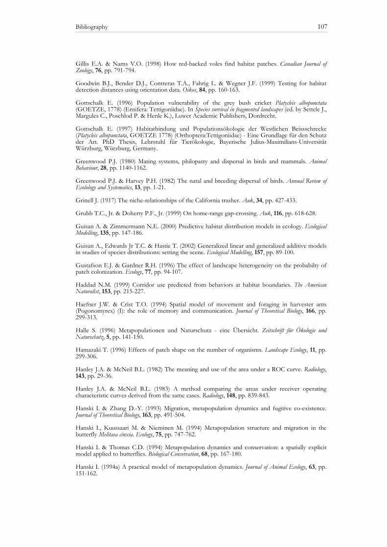
Bibliography 107
Gillis E.A. & Nams V.O. (1998) How red-backed voles find habitat patches. Canadian Journal of Zoology, 76, pp. 791-794. Goodwin B.J., Bender D.J., Contreras T.A., Fahrig L. & Wegner J.F. (1999) Testing for habitat detection distances using orientation data. Oikos, 84, pp. 160-163. Gottschalk E. (1996) Population vulnerability of the grey bush cricket Platycleis albopunctata (GOETZE, 1778) (Ensifera: Tettigoniidae). In Species survival in fragmented landscapes (ed. by Settele J., Margules C., Poschlod P. & Henle K.), Luwer Academic Publishers, Dordrecht. Gottschalk E. (1997) Habitatbindung und Populationsökologie der Westlichen Beissschrecke (Platycleis albopunctata, GOETZE 1778) (Orthoptera:Tettigoniidae) - Eine Grundlage für den Schutz der Art. PhD Thesis, Lehrstuhl für Tierökologie, Bayerische Julius-Maximilians-Universität Würzburg, Würzburg, Germany. Greenwood P.J. (1980) Mating systems, philopatry and dispersal in birds and mammals. Animal Behaviour, 28, pp. 1140-1162. Greenwood P.J. & Harvey P.H. (1982) The natal and breeding dispersal of birds. Annual Review of Ecolology and Systematics, 13, pp. 1-21. Grinell J. (1917) The niche-relationships of the California trasher. Auk, 34, pp. 427-433. Grubb T.C., Jr. & Doherty P.F., Jr. (1999) On home-range gap-crossing. Auk, 116, pp. 618-628. Guisan A. & Zimmermann N.E. (2000) Predictive habitat distribution models in ecology. Ecological Modelling, 135, pp. 147-186. Guisan A., Edwards Jr T.C. & Hastie T. (2002) Generalized linear and generalized additive models in studies of species distributions: setting the scene. Ecological Modelling, 157, pp. 89-100. Gustafson E.J. & Gardner R.H. (1996) The effect of landscape heterogeneity on the probabilty of patch colonization. Ecology, 77, pp. 94-107. Haddad N.M. (1999) Corridor use predicted from behaviors at habitat boundaries. The American Naturalist, 153, pp. 215-227. Haefner J.W. & Crist T.O. (1994) Spatial model of movement and foraging in harvester ants (Pogonomyrex) (I): the role of memory and communication. Journal of Theoretical Biology, 166, pp. 299-313. Halle S. (1996) Metapopulationen und Naturschutz - eine Übersicht. Zeitschrift für Ökologie und Naturschutz, 5, pp. 141-150. Hamazaki T. (1996) Effects of patch shape on the number of organisms. Landscape Ecology, 11, pp. 299-306. Hanley J.A. & McNeil B.L. (1982) The meaning and use of the area under a ROC curve. Radiology, 143, pp. 29-36. Hanley J.A. & McNeil B.L. (1983) A method comparing the areas under receiver operating characteristic curves derived from the same cases. Radiology, 148, pp. 839-843. Hanski I. & Zhang D.-Y. (1993) Migration, metapopulation dynamics and fugitive co-existence. Journal of Theoretical Biology, 163, pp. 491-504. Hanski I., Kuussaari M. & Nieminen M. (1994) Metapopulation structure and migration in the butterfly Melitaea cinxia. Ecology, 75, pp. 747-762. Hanski I. & Thomas C.D. (1994) Metapopulation dynamics and conservation: a spatially explicit model applied to butterflies. Biological Conservation, 68, pp. 167-180. Hanski I. (1994a) A practical model of metapopulation dynamics. Journal of Animal Ecology, 63, pp. 151-162.

Bibliography 108
Hanski I. (1994b) Patch-occupancy dynamics in fragmented landscapes. Tree, 9, pp. 131-135. Hanski I. & Gilpin M.E. (1997) Metapopulation biology: ecoloy, genetics and evolution. Academic Press, San Diego, California. Hanski I. (2001) Population dynamic consequences of dispersal in local populations and in metapopulations. In Dispersal (ed. by Oxford University Press, Oxford. Hansson L. (1991) Dispersal and connectivity in metapopulations. In Metapopulation Dynamics (ed. by Gilpin M.E. & Hanski I.), Academic Press, London. Harrell F.E.J. (2001) Regression modeling strategies: with applications to linear models, logistic regression, and survival analysis. Springer-Verlag, Harrison S. (1989) Long-distance dispersal and colonization in the Bay checkerspot butterfly, Euphydryas bayensis. Ecology, 70, pp. 1236-1243. Harrison S. (1991) Local extinction in a metapopulation context: an empirical evaluation. Biological Journal of the Linnean Society of London, 42, pp. 73-88. Hartley J.C. & Warne A.C. (1972) The developmental biology of the egg stage of Western European Tettigoniidae (Orthoptera). Journal of Zoology, 168, pp. 267-298. Harz K. (1969) The Orthoptera of Europa. The Hague, Haupt H. (1995) Faunistische Beobachtungen an Heuschrecken (Orthoptera: Saltatoria) im Unteren Odertal bei Schwedt (Brandenburg) mit einem Wiederfund von Platycleis montana KOLLAR, 1833. Articulata, 8, pp. 83-87. Heglund P.J., Jones J.R., Fredrickson L.H. & Kaise M.S. (1994) Use of boreal forested wetlands by Pacific loons (Gavia pacifica Lawrence) and horned grebes (Podiceps auritus L.): Relations with limnological characteristics. Hydrobiologia, 279/280, pp. 171-183. Heglund P.J. (2002) Foundations of Species-Environment Relations. In Predicting species occurrences (ed. by Scott J.M., Heglund P.J., Morrision M.L., Haufler J.B., Raphael M.G., Wall W.A. & Samson F.B.), Island Press, Washington. Hein S., Gombert J., Hovestadt T. & Poethke H.J. (2003) Movement patterns of Platycleis albopunctata in different types of habitat: matrix is not always matrix. Ecological Entomology, 28, pp. 432-438. Hein S., Pfenning B., Hovestadt T. & Poethke H.J. (in press) Patch density, movement pattern, and realized dispersal distances in a patch-matrix landscape - a simulation study. Ecological Modelling, pp. Heinrich W., Marstaller R., Bährmann R., Perner J. & Schäller G. (1998) Naturschutzreport - Jena: Das Naturschutzgebiet "Leutratal" bei Jena - Struktur- und Sukzessionsforschung in Grasland-Ökosystemen. Jena. Heller K.-G. & von Helversen O. (1990) Survival of a Phaneropterid bush-cricket studied by a new marking technique (Orthoptera: Phaneropteridae). Entomologica Generalis, 15, pp. 203-208. Hensle J. (1995) Fund einer Herbstgeneration von Coenonympha arcania im Elsaß. Nachrichten des entomologischen Vereins Apollo, 16, pp. 28. Higgins S.I. & Richardson D.M. (1999) Predicting plant migration rates in a changing world: the role of long-distance dispersal. American Naturalist, 153, pp. 464-475. Hill J.K., Thomas C.D. & Lewis O.T. (1996) Effects of habitat patch size and isolation on dispersal by Hesperia comma butterflies: implications for metapopulation structure. Journal of Animal Ecology, 65, pp. 725-735. Hinch S.G., Somers K.M. & Collins N.C. (1994) Spatial autocorrelation and assessment of habitat-abundance relationships in littoral zone fish. Canadian Journal of Fisheries and Aquatic Sciences, 51, pp. 701-712.
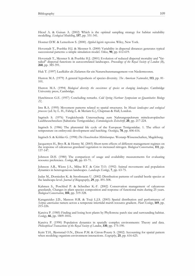
Bibliography 109
Hirzel A. & Guisan A. (2002) Which is the optimal sampling strategy for habitat suitability modelling. Ecological Modelling, 157, pp. 331-341. Hosmer D.W. & Lemeshow S. (2000) Applied logistic regression. Wiley, New York. Hovestadt T., Poethke H.J. & Messner S. (2000) Variability in dispersal distances generates typical successional patterns: a simple simulation model. Oikos, 90, pp. 612-619. Hovestadt T., Messner S. & Poethke H.J. (2001) Evolution of reduced dispersal mortality and "fat-tailed" dispersal functions in autocorrelated landscapes. Proceedings of the Royal Society of London (B), 268, pp. 385-391. Huk T. (1997) Laufkäfer als Zielarten für ein Naturschutzmanagement von Niedermooren. Huston M.A. (1979) A general hypothesis of species diversity. The American Naturalist, 113, pp. 81-101. Huston M.A. (1994) Biological diversity the coexistence of species on changing landscapes. Cambridge University press, Cambridge. Hutchinson G.E. (1957) Concluding remarks. Cold Spring Harbour Symposium on Quantitative Biology 22, Ims R.A. (1995) Movement patterns related to spatial structures. In Mosaic landscapes and ecological processes (ed. by L. H., Fahrig L. & Meriam G.), Chapman & Hall, London. Ingrisch S. (1976) Vergleichende Untersuchung zum Nahrungsspektrum mitteleuropäischer Laubheuschrecken (Saltatoria: Tettigoniidae). Entomologische Zeitschrift, 20, pp. 217-224. Ingrisch S. (1986) The plurennial life cycle of the European Tettigoniidae. 1. The effect of temperature on embryonic development and hatching. Oecologia, 70, pp. 606-616. Ingrisch S. & Köhler G. (1998) Die Heuschrecken Mitteleuropas. Westarp-Wissenschaften, Magdeburg. Jacquemyn H., Brys R. & Hermy M. (2003) Short-term effects of different management regimes on the response of calcareous grassland vegetation to increased nitrogen. Biological Conservation, 111, pp. 137-147. Johnson D.H. (1980) The comparison of usage and availability measurements for evaluating resource preference. Ecology, 61, pp. 65-71. Johnson A.R., Wiens J.A., Milna B.T. & Crist T.O. (1992) Animal movements and population dynamics in heterogeneous landscapes. Landscape Ecology, 7, pp. 63-75. Judas M., Dornieden K. & Strothmann U. (2002) Distribution patterns of carabid beetle species at the landscape-level. Journal of Biogeography, 29, pp. 491-508. Kahmen S., Poschlod P. & Schreiber K.-F. (2002) Conservation management of calcareous grasslands. Changes in plant species composition and response of functional traits during 25 years. Biological Conservation, 104, pp. 319-328. Karagatzides J.D., Manson H.R. & Tsuji L.J.S. (2003) Spatial distribution and performance of Scirpus americanus ramets across a temperate intertidal marsh resource gradient. Plant Ecology, 169, pp. 215-226. Kareiva P. (1985) Finding and losing host plants by Phyllotreta: patch size and surrounding habitat. Ecology, 66, pp. 1809-1816. Kareiva P. (1990) Population dynamics in spatially complex environments: Theory and data. Philosophical Transactions of the Royal Society of London, 330, pp. 175-190. Keitt T.H., Bjornstad O.N., Dixon P.M. & Citron-Pousty S. (2002) Accounting for spatial pattern when modeling organism-environment interactions. Ecography, 25, pp. 616-625.
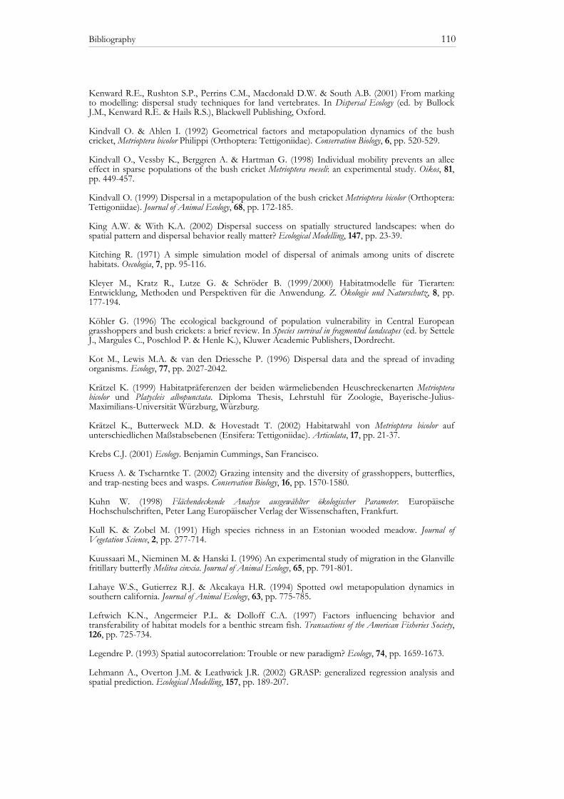
Bibliography 110
Kenward R.E., Rushton S.P., Perrins C.M., Macdonald D.W. & South A.B. (2001) From marking to modelling: dispersal study techniques for land vertebrates. In Dispersal Ecology (ed. by Bullock J.M., Kenward R.E. & Hails R.S.), Blackwell Publishing, Oxford. Kindvall O. & Ahlen I. (1992) Geometrical factors and metapopulation dynamics of the bush cricket, Metrioptera bicolor Philippi (Orthoptera: Tettigoniidae). Conservation Biology, 6, pp. 520-529. Kindvall O., Vessby K., Berggren A. & Hartman G. (1998) Individual mobility prevents an allee effect in sparse populations of the bush cricket Metrioptera roeseli: an experimental study. Oikos, 81, pp. 449-457. Kindvall O. (1999) Dispersal in a metapopulation of the bush cricket Metrioptera bicolor (Orthoptera: Tettigoniidae). Journal of Animal Ecology, 68, pp. 172-185. King A.W. & With K.A. (2002) Dispersal success on spatially structured landscapes: when do spatial pattern and dispersal behavior really matter? Ecological Modelling, 147, pp. 23-39. Kitching R. (1971) A simple simulation model of dispersal of animals among units of discrete habitats. Oecologia, 7, pp. 95-116. Kleyer M., Kratz R., Lutze G. & Schröder B. (1999/2000) Habitatmodelle für Tierarten: Entwicklung, Methoden und Perspektiven für die Anwendung. Z. Ökologie und Naturschutz, 8, pp. 177-194. Köhler G. (1996) The ecological background of population vulnerability in Central European grasshoppers and bush crickets: a brief review. In Species survival in fragmented landscapes (ed. by Settele J., Margules C., Poschlod P. & Henle K.), Kluwer Academic Publishers, Dordrecht. Kot M., Lewis M.A. & van den Driessche P. (1996) Dispersal data and the spread of invading organisms. Ecology, 77, pp. 2027-2042. Krätzel K. (1999) Habitatpräferenzen der beiden wärmeliebenden Heuschreckenarten Metrioptera bicolor und Platycleis albopunctata. Diploma Thesis, Lehrstuhl für Zoologie, Bayerische-Julius-Maximilians-Universität Würzburg, Würzburg. Krätzel K., Butterweck M.D. & Hovestadt T. (2002) Habitatwahl von Metrioptera bicolor auf unterschiedlichen Maßstabsebenen (Ensifera: Tettigoniidae). Articulata, 17, pp. 21-37. Krebs C.J. (2001) Ecology. Benjamin Cummings, San Francisco. Kruess A. & Tscharntke T. (2002) Grazing intensity and the diversity of grasshoppers, butterflies, and trap-nesting bees and wasps. Conservation Biology, 16, pp. 1570-1580. Kuhn W. (1998) Flächendeckende Analyse ausgewählter ökologischer Parameter. Europäische Hochschulschriften, Peter Lang Europäischer Verlag der Wissenschaften, Frankfurt. Kull K. & Zobel M. (1991) High species richness in an Estonian wooded meadow. Journal of Vegetation Science, 2, pp. 277-714. Kuussaari M., Nieminen M. & Hanski I. (1996) An experimental study of migration in the Glanville fritillary butterfly Melitea cinxia. Journal of Animal Ecology, 65, pp. 791-801. Lahaye W.S., Gutierrez R.J. & Akcakaya H.R. (1994) Spotted owl metapopulation dynamics in southern california. Journal of Animal Ecology, 63, pp. 775-785. Leftwich K.N., Angermeier P.L. & Dolloff C.A. (1997) Factors influencing behavior and transferability of habitat models for a benthic stream fish. Transactions of the American Fisheries Society, 126, pp. 725-734. Legendre P. (1993) Spatial autocorrelation: Trouble or new paradigm? Ecology, 74, pp. 1659-1673. Lehmann A., Overton J.M. & Leathwick J.R. (2002) GRASP: generalized regression analysis and spatial prediction. Ecological Modelling, 157, pp. 189-207.
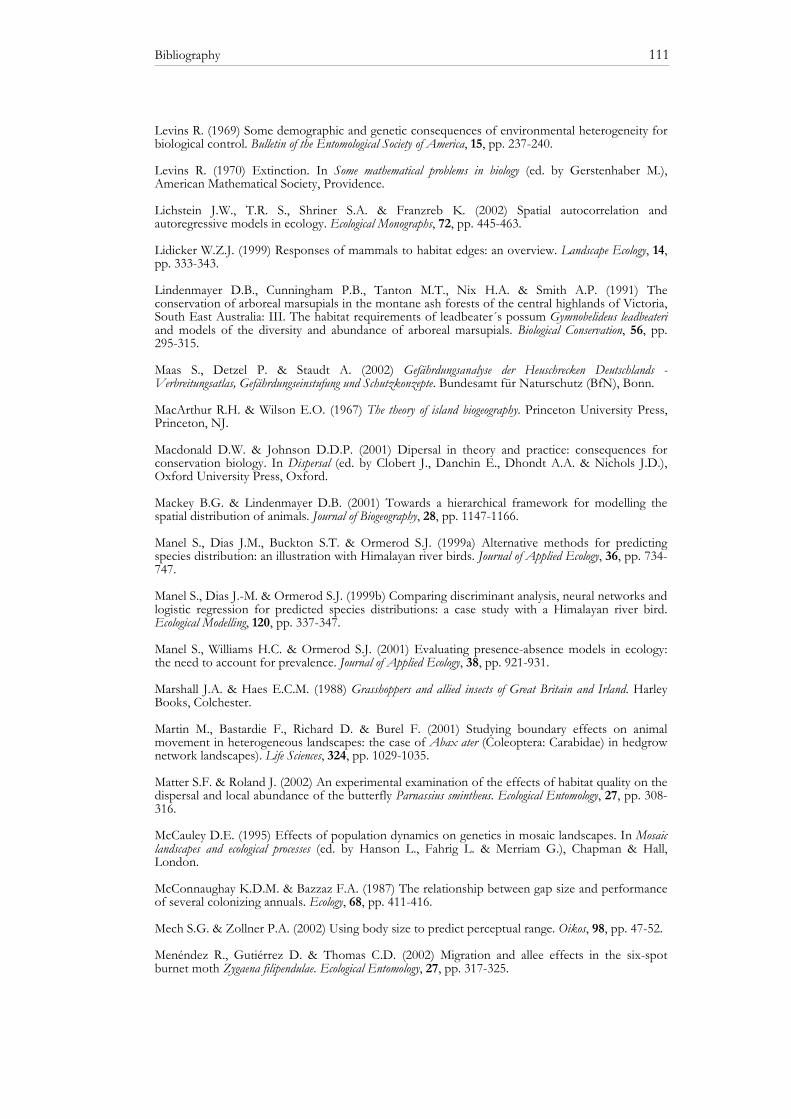
Bibliography 111
Levins R. (1969) Some demographic and genetic consequences of environmental heterogeneity for biological control. Bulletin of the Entomological Society of America, 15, pp. 237-240. Levins R. (1970) Extinction. In Some mathematical problems in biology (ed. by Gerstenhaber M.), American Mathematical Society, Providence. Lichstein J.W., T.R. S., Shriner S.A. & Franzreb K. (2002) Spatial autocorrelation and autoregressive models in ecology. Ecological Monographs, 72, pp. 445-463. Lidicker W.Z.J. (1999) Responses of mammals to habitat edges: an overview. Landscape Ecology, 14, pp. 333-343. Lindenmayer D.B., Cunningham P.B., Tanton M.T., Nix H.A. & Smith A.P. (1991) The conservation of arboreal marsupials in the montane ash forests of the central highlands of Victoria, South East Australia: III. The habitat requirements of leadbeater´s possum Gymnobelideus leadbeateri and models of the diversity and abundance of arboreal marsupials. Biological Conservation, 56, pp. 295-315. Maas S., Detzel P. & Staudt A. (2002) Gefährdungsanalyse der Heuschrecken Deutschlands - Verbreitungsatlas, Gefährdungseinstufung und Schutzkonzepte. Bundesamt für Naturschutz (BfN), Bonn. MacArthur R.H. & Wilson E.O. (1967) The theory of island biogeography. Princeton University Press, Princeton, NJ. Macdonald D.W. & Johnson D.D.P. (2001) Dipersal in theory and practice: consequences for conservation biology. In Dispersal (ed. by Clobert J., Danchin E., Dhondt A.A. & Nichols J.D.), Oxford University Press, Oxford. Mackey B.G. & Lindenmayer D.B. (2001) Towards a hierarchical framework for modelling the spatial distribution of animals. Journal of Biogeography, 28, pp. 1147-1166. Manel S., Dias J.M., Buckton S.T. & Ormerod S.J. (1999a) Alternative methods for predicting species distribution: an illustration with Himalayan river birds. Journal of Applied Ecology, 36, pp. 734-747. Manel S., Dias J.-M. & Ormerod S.J. (1999b) Comparing discriminant analysis, neural networks and logistic regression for predicted species distributions: a case study with a Himalayan river bird. Ecological Modelling, 120, pp. 337-347. Manel S., Williams H.C. & Ormerod S.J. (2001) Evaluating presence-absence models in ecology: the need to account for prevalence. Journal of Applied Ecology, 38, pp. 921-931. Marshall J.A. & Haes E.C.M. (1988) Grasshoppers and allied insects of Great Britain and Irland. Harley Books, Colchester. Martin M., Bastardie F., Richard D. & Burel F. (2001) Studying boundary effects on animal movement in heterogeneous landscapes: the case of Abax ater (Coleoptera: Carabidae) in hedgrow network landscapes). Life Sciences, 324, pp. 1029-1035. Matter S.F. & Roland J. (2002) An experimental examination of the effects of habitat quality on the dispersal and local abundance of the butterfly Parnassius smintheus. Ecological Entomology, 27, pp. 308-316. McCauley D.E. (1995) Effects of population dynamics on genetics in mosaic landscapes. In Mosaic landscapes and ecological processes (ed. by Hanson L., Fahrig L. & Merriam G.), Chapman & Hall, London. McConnaughay K.D.M. & Bazzaz F.A. (1987) The relationship between gap size and performance of several colonizing annuals. Ecology, 68, pp. 411-416. Mech S.G. & Zollner P.A. (2002) Using body size to predict perceptual range. Oikos, 98, pp. 47-52. Menéndez R., Gutiérrez D. & Thomas C.D. (2002) Migration and allee effects in the six-spot burnet moth Zygaena filipendulae. Ecological Entomology, 27, pp. 317-325.
Bibliography 112
Meriam G. (1991) Corridors and connectivity: animal populations in heterogeneous environments. In Nature conservation 2: the role of corridors (ed. by Saunders D.A. & Hobbs R.J.), Surrey Beatty & Sons, Chipping Norton, NSW. Merkel E. (1980) Sandtrockenstandorte und ihre Bedeutung für zwei "Ödland"-Schrecken der Roten Liste. Schriftenreihe Naturschutz und Landschaftspflege, 12, pp. 63-69. Metz J.A.A. & Gyllenberg M. (2001) How should we define fitness in structured metapopulation models? Including an application to the calculation of evolutionary stable dispersal strategies. Proceedings of the Royal Society of London (B), 268, pp. 499-508. Moilanen A. & Hanski I. (1998) Metapopulation dynamics: effects of habitat quality and landscape structure. Ecology, 79, pp. 2503-2515. Moilanen A. & Hanski I. (2001) On the use of connectivity measures in spatial ecology. Oikos, 95, pp. 147-151. Moilanen A. & Nieminen M. (2002) Simple connectivity measures in spatial ecology. Ecology, 83, pp. 1131-1145. Morrison M.L., Marcot B.G. & Mannan R.W. (1998) Wildlife-habitat relationsships - concepts and applications. The University of Wisconsin Press, Madison. Mortimer S.R., Hollier J.A. & Brown V.K. (1998) Interactions between plant and insect diversity in the restoration of lowland calcareous grasslands in southern Britain. Applied Vegetation Science, 1, pp. 101-114. Mühlenberg M. (1993) Freilandökologie. UTB, Heidelberg. Mühlenberg M., Henle K., Settele J., Poschlod P., Seitz A. & Kaule G. (1996) Studying species survival in fragmented landscapes: The approach of the FIFB. In Species survival in fragmented landscapes (ed. by Settele J., Margules C., Poschlod P. & Henle K.), Kluwer Academic Publishers, Dordrecht. Nadig A. & Thorens P. (1994) Rote Liste der gefährdeten Heuschrecken der Schweiz. In Rote Listen der gefährdeten Tierarten der Schweiz (ed. by Duelli P.), Bundesamt für Umwelt, Wald und Landschaft, Bern. Nagelkerke N.J.D. (1991) A note on a general definition of the coefficient of determination. Biometrika, 78, pp. 691-692. Nève G., Barascud B., Hughes R.M., Aubert J., Descimon H., Lebrun P. & Baguette M. (1996a) Dispersal, colonisation power and metapopulation structure in the vulnerable butterfly Proclossiana eunomia (Lepidoptera, Nymphalidae). Journal of Applied Ecology, 33, pp. 14-22. Nève G., Mousson L. & Baguette M. (1996b) Adult dispersal and genetic structure of butterfly populations in a fragmented landscape. Acta Ecologia, 17, pp. 621-626. New T.R. (1995) An introduction to invertebrate conservation biology. Oxford University Press, Oxford. New T.R., Pyle R.M., Thomas J.A., Thomas C.D. & Hammond P.C. (1995) Butterfly conservation management. Annual Review of Entomology, 40, pp. Nieminen M. (1996) Migration of moth species in a network of small islands. Oecologia, 108, pp. 643-651. Noss R.F. (1990) Indicators for monitoring biodiversity: a hierarchical approach. Conservation Biology, 4, pp. 355-364. Nottingham S.F. (1988) Host plant finding for oviposition by adult cabbage root fly, Delia radicum. Journal of Insect Physiology, 34, pp. 227-234. Oostermeijer J.G.B., Berholz A. & Poschlod P. (1996) Genetical aspects of fragmented plant populations. In Species survival in fragmented landscapes (ed. by Settele J., Margules C., Poschlod P. & Henle K.), Kluwer Academic Publishers, Dordrecht.

Bibliography 113
Opdam P. (1990) Dispersal in fragmented populations: the key to survival. In Species dispersal in agricultural habitats (ed. by Bunce R.G.H. & Howard D.C.), Belhaven Press, New York. Opitz S., Köhler G. & Mabelis A. (1998) Local movement of the grasshopper Chorthippus parallelus (Zett.). Proceedings of Experimental and Applied Entomology, 9, pp. 53-57. Oppel S., Schaefer H.M., Schmidt V. & Schröder B. (in press) Habitat selection by the pale-headed brush-finch (Atlapetes pallidiceps) in southern Ecuador: implications of conservation. Biological Conservation, pp. Orians G.H. & Wittenberger J.F. (1991) Spatial and temporial scales in habitat selection. American Naturalist, 137, pp. 29-49. Osborne P.E., Alonso J.C. & Bryant R.G. (2001) Modelling landscape-scale habitat use using GIS and remote sensing: a case study with great bustards. Journal of Applied Ecology, 38, pp. 458-471. Oschmann M. (1993) Artunterschiede in der Phänologie der Heuschrecken (Saltatoria). Articulata, 8, pp. 35-43. Ovaskainen O. & Hanski I. (2001) Spatially structured metapopulation models: global and local assessment of metapopulation capacity. Theoretical Population Biology, 60, pp. 281-302. Paradis E., Baillie S.R. & Sutherland W.J. (2002) Modeling large-scale dispersal distances. Ecological Modelling, 151, pp. 279-292. Pearce J.L., Burgman M.A. & Franklin D.C. (1994) Habitat selection by helmeted honeyeater. Wildlife Research, 21, pp. 53-63. Pearce J. & Ferrier S. (2000a) An evaluation of alternative algorithms for fitting species distribution models using logistic regression. Ecological modelling, 128, pp. 127-147. Pearce J. & Ferrier S. (2000b) Evaluating the predictive performance of habitat models developed using logistic regression. Ecological modelling, 133, pp. 225-245. Poethke H.J., Gottschalk E. & Seitz A. (1996a) Gefährdungsgradanalyse einer räumlich strukturierten Population der westlichen Beißschrecke (Platycleis albopunctata): Ein Beispiel für den Einsatz des Metapopulationskonzeptes im Artenschutz. Zeitschrift für Ökologie und Naturschutz, 5, pp. 229-242. Poethke H.J., Seitz A. & Wissel C. (1996b) Species survival and metapopulations: conservation implications from ecological theory. In Species survival in fragmented landscapes (ed. by Settele J., Margules C., Poschlod P. & Henle K.), Kluwer Academic Publishers, London. Poethke H.J. & Hovestadt T. (2002) Evolution of density and patch-size dependent dispersal rates. Proceedings of the Royal Society of London (B), 269, pp. 637-645. Poethke A., Hovestadt T. & Mitesser O. (2003) Local extinction and the evolution of dispersal rates: causes and correlations. American Naturalist, 161, pp. 631-640. Portnoy S. & Willson M.F. (1993) Seed dispersal curves - behavior of the tail of the distribution. Evolutionary Ecology, 7, pp. 25-44. Poschlod P., Bakker J., Bonn S. & Fischer S. (1996) Dispersal of plants in fragmented landscapes. In Species survival in fragmented landscapes (ed. by Settele J., Margules C., Poschlod P. & Henle K.), Kluwer Academic Publishers, Dordrecht. Poschlod P. & Schumacher W. (1998) Rückgang von Pflanzen - und Pflanzengeseellschaften des Grünlandes.- Gefährdungsursachen und Handlungsbedarf. Schriftenreihe für Vegetationskunde, 29, pp. 83-99. Pulliam H.R. (1988) Source, sinks, and population regulation. American Naturalist, 132, pp. 652-661. Pulliam H.R., Dunning J.B. & Liu J.G. (1992) Population-dynamics in complex landscapes - a case study. Ecological Applications, 2, pp. 165-177.

Bibliography 114
Pykälä J. (2003) Effects of restoration with cattle grazing on plant species composition and richness of semi-natural grasslands. Biodiversity and Conservation, 12, pp. 2211-2226. Reich M. & Grimm V. (1996) Das Metapopulationskonzept in Ökologie und Naturschutz: Eine kritische Bestandsaufnahme. Zeitschrift für Ökologie und Naturschutz, 5, pp. 123-139. Reineking B. & Schröder B. (2003) Computer-intensive methods in the analysis of species-habitat relationships. Proceedings "Genes, Bits and Ecosystems" Theory in Ecology, Frankfurt. Rice W. (1989) Analyzing tables of statistical tests. Evolution, 43, pp. 223-225. Ricketts T.H. (2001) The matrix matters: Effective Isolation in Fragmented Landscapes. American Naturalist, 158, pp. 87-99. Riegert P.W., Fuller R.A. & Putnam L.G. (1954) Studies on dispersal of grasshoppers (Acrididae) tagged with phosphorus-32. The Canadian Entomologist, 86, pp. 223-232. Roland J., Keyghobadi N. & Fownes S. (2000) Alpine Parnassius butterfly dispersal: effects of landscape and population size. Ecology, 81, pp. 1642-1653. Ronce O., Gandon S. & Rousset F. (2000) Kin selection and natal dispersal in an age-structured population. Theoretical Population Biology, 58, pp. 143-159. Root R.B. & Kareiva P.M. (1984) The search for resources by cabbage butterfly (Pieris rapae): ecological consequences and adaptive significance of Markovian movements in a patchy environment. Ecology, 65, pp. 147-165. Rosenzweig M.L. (1981) A theory of habitat selection. Ecology, 62, pp. 327-335. Rosenzweig M.L. (1995) Species diversity in space and time. Cambridge University Press, Cambridge. Roslin T. (2000) Dung beetle movements at two spatial scales. Oikos, 91, pp. 323-335. Rutte E. (1981) Bayerns Erdgeschichte. Der geologische Führer durch Bayern. Ehrenwirth, München. Samietz J., Berger U. & Köhler G. (1996) A population vulnerability analysis of the stripe-winged grasshopper, Stenobothrus lineatus (Caelifera: Acrididae). In Species survival in fragmented landscapes (ed. by Settele J., Margules C., Poschlod P. & Henle K.), Kluwer Academic Publishers, Dordrecht. Samietz J. & Berger U. (1997) Evaluation of movement parameters in insects - bias and robustness with regard to resight numbers. Oecologia, 110, pp. 40-49. Samietz J. (1998) Populationsgefährdungsanalyse an einer Heuschreckenart - Methoden, empirische Grundlagen und Modellbildung bei Stenobothrus lineatus (Panzer). Göttingen. Schooley R.L. & Wiens J.A. (2003) Finding habitat patches and directional connectivity. Oikos, 102, pp. 559-570. Schreiber K.F. (1977) Zur Sukzession und Flächenfreihaltung auf Brachland in Baden-Württemberg. Verhandlungen der Gesellschaft für Ökologie, Göttingen. Schröder B. & Richter O. (1999) Are habitat models transferable in space and time? Zeitschrift für Ökologie und Naturschutz, 8, pp. 195-205. Schröder B. (2000) Zwischen Naturschutz und Theoretischer Ökologie: Modelle zur Habitateignung und räumlichen Populationsdynamik für Heuschrecken im Niedermoor. PhD thesis, Institut für Geographie und Geoökologie der Technischen Universität Braunschweig, Technische Universität Braunschweig, Braunschweig. Schröder B., Biedermann R. & Kleyer M. (2003) Ecological and socio-economic assessment of management systems for open landscapes - an integrated landscape model approach.
Bibliography 115
Schröder B., Rudner M., Biedermann R. & Kleyer M. (2003) Ökologische & sozio-ökonomische Bewertung von Managementsystemen für die Offenhaltung von Landschaften - ein integriertes Landschaftsmodell. UFZ Berichte, in press, pp. Schultz C.B. (1998) Dispersal behavior and its implications for reserve design in a rare Oregon butterfly. Conservation biology, 12, pp. 284-292. Schultz C.B. & Crone E.E. (2001) Edge-mediated dispersal behavior in a prairie butterfly. Ecology, 82, pp. 1879-1892. Settele J. & Poethke A. (1996) Towards demographic population vulnerability categories of butterflies: Requirements of and species selection for future population ecological research. In Species survival in fragmented landscapes (ed. by Settele J., Margules C., Poschlod P. & Henle K.), Kluwer Academic Publishers, Dodrecht. Settele J. (1998) Metapopulationsanalyse auf Rasterdatenbasis. B.G. Teubner Verlagsgesellschaft, Stuttgart. Settele J., Feldmann R. & Reinhardt R. (1999) Die Tagfalter Deutschlands - Ein Handbuch für Freilandökologen, Umweltplaner und Naturschützer. Ulmer Verlag, Stuttgart. Simberloff D. (1998) Flagships, umbrellas, and keystones: is single species management passé in the landscape era? Biological Conservation, 83, pp. 247-257. Smith P.A. (1994) Autocorrelation in logistic regression modelling of species´ distributions. Global Ecology and Biogeography letters, 4, pp. 47-61. Söderström B. & Pärt T. (2000) Influence of landscape scale on farmland birds in seminatural pastures. Conservation Biology, 14, pp. 522-533. Söderström B., Svensson B., Vessby K. & Glimskär A. (2001) Plants, insects and birds in semi-natural pastures in relation to local habitat and landscape factors. Biodiversity and Conservation, 10, pp. 1839-1863. South A. (1999) Dispersal in spatially explicit population models. Conservation Biology, 13, pp. 1039-1046. South A.B., Rushton S.P., Kenward R.E. & Macdonald D.W. (2002) Modelling vertebrate dispersal and demography in real landscapes: how does uncertainty regarding dispersal behaviour influence predictions of spatial population dynamics? In Dispersal Ecology (ed. by Bullock J.M., Kenward R.E. & Hails R.S.), Blackwell publishing, Oxford. Stenseth N.C. (1983) Causes and consequences of dispersal in small mammals. In The Ecology of Animal Movement (ed. by Swingland I.R. & Greenwood P.J.), Clarendon Press, Oxford. Stettmer C. (1996) Colonisation and dispersal patterns of banded (Calopteryx splendens) and beautifull demoiselles (C. virgo) (Odonata: Calopteryidae) in south-east German streams. EuropeanJournal of Entomology, 93, pp. 579-593. Storch I. (2002) On spatial resolution in habitat models: Can small-scale forest structure explain Capercaillie numbers? Conservation Ecology, 6. online., pp. Sundermeier A. (1999) Zur Vegetationsdichte der Xerothermrasen nordwestlich von Halle/Saale. Cramer, J., Stuttgart, Germany. Sutcliffe O.L., Thomas C.D. & Peggie D. (1997) Area-dependent migration by ringlet butterflies generates mixture of patchy population and metapopulation attributes. Oecologia, 109, pp. 229-234. Taylor A.D. (1990) Metapopulations, dispersal, and predator-prey dynamics: an overview. Ecology, 71, pp. 429-433. Thomas C.D. & Hanski I. (1997) Butterfly Metapopulations. In Metapopulation Biology (ed. by Hanski I. & Gilpin M.E.), Academic Press, London.

Bibliography 116
Thomas J.A., Bourn N.A.D., Clarke R.T., Stewart K.E., Simcox D.J., Pearman G.S., Curtis R. & Goodger B. (2001) The quality and isolation of habitat patches both determine where butterflies persist in fragmented landscapes. Proceedings of the Royal Society London, 268, pp. 1791-1796. Travis J.M., Murell D.J. & Dythamn C. (1999) The evolution of density-dependent dispersal. Proceedings of the Royal Society of London (B), 266, pp. 1837-1842. Trexler J.C. & Travis J. (1993) Nontraditional regression analyses. Ecology, 74, pp. 1629-1637. Turchin P. (1991) Translating foraging movements in the heterogeneous environments into the spatial distribution of foragers. Ecology, 72, pp. 1253-1266. Turchin P. (1998) Quantitative analysis of movement: Measuring and modeling population redistribution in animals and plants. Sinauer Associates, Massachusetts. Turner M.G., Wu Y., Romme W.H. & Wallace L.L. (1993) A landscape simulation model of winter foraging by large ungulates. Ecological Modelling, 69, pp. 163-184. U.S. Fish & Wildlife Service (1981) Habitat evaluation procedures (HEP). U.S. Department of the Interior, U.S, Fish and Wildlife Service, Division of Ecological Services, Washington, D.C,. van der Maarel E. & Titlyanova A. (1989) Above-ground and below-ground biomass related in steppes under different grazing conditions. Oikos, 56, pp. 364-370. Van Dijk G. (1991) The status of semi-natural grasslands in Europe. In The conservation of lowland dry grassland birds in Europe (ed. by Goriup P.D., Batten L.A. & Norton J.A.), Joint Nature Conservation Committee, Peterborough. van Wingerden W.K.R.E., Musters J.C.M. & Maascamp F.I.M. (1991) The influence of temperature on the duration of egg development in West European grasshoppers (Orthoptera: Acrididae). Oecologia, 87, pp. 417-423. Veith M. & Klein M. (1996) Zur Anwendung des Metapopulationskonzeptes auf Amphibienpopulationen. Zeitschrift für Ökologie und Naturschutz, 5, pp. 217-228. Verbyla D.L. & Litvaitis J.A. (1989) Resampling Methods for evaluating classification accuracy of wildlife habitat models. Environmental Managment, 13, pp. 783-787. Verner J., Morrision M.L. & Ralph C.J. (1986) Wildlife 2000: Modeling habitat relationships of terrestrial vertebrates. University of Wisconsin Press, Madison, Wisconsin. Villard M.A., Trzcinski M.K. & Merriam G. (1999) Fragmentation effects on forest birds: relative influence of woodland cover and configuration on landscape occupancy. Conservation Biology, 13, pp. 774-783. Vos C.C. & Zonnefeld J.I.S. (1993) Patterns and processes in a landscape under stress: the study area. In Landscape Ecology of a Stressed Environment (ed. by Vos C.C. & Opdam P.), Chapmann & Hall, London. Walter R. (1992) Untersuchungen zur Mobilität und zum Habitat von Platycleis albopunctata (GOETZE 1778) (Orthoptera, Ensifera). Diplomathesis, Fakultät für Biologie der Universität Hohenheim, Hohenheim, Germany. Walter M. (1994) Untersuchungen zur Nahrungsökologie der Westlichen Beißschrecke Platycleis albopunctata (Orthoptera: Tettigoniidae). Diploma Thesis, University of Würzburg, Würzburg. Weidemann H.J. (1995) Tagfalter: beobachten, bestimmen. Naturbuch Verlag, Augsburg. Wessels K.J., van Jaarsveld A.S., Grimbeek J.D. & van der Linde M.J. (1998) An evaluation of the gradsect biological survey method. Biodiversity and Conservation, 7, pp. 1093-1121. Wiegand T., Moloney K.A., Naves J. & Knauer F. (1999) Finding the missing link between landscape structure and population dynamics: a spatially explicit perspective. American Naturalist, 154, pp. 605-627.
Bibliography 117
Wiens J.A. (1989) The ecology of bird communities. Cambridge Univrsity Press, Cambrdige. Wiens J.A. & Milne B.T. (1989) Scaling of "landscapes" in landscape ecology, or landscape ecology from beetle´s perspective. Landscape ecology, 3, pp. 87-96. Wiens J.A., Crist T.O. & Milne B.T. (1993) On quantifying insect movements. Environmental Entomology, 22, pp. 710-715. Wiens J.A., Stenseth N.C., Van Horne B. & Ims R.A. (1993) Ecological mechanisms and landscape ecology. Oikos, 66, pp. 369-380. Wiens J.A., Schooley R.L. & Weeks R.D. (1997) Patchy landscapes and animal movements: Do beetles percolate ? Oikos, 78, pp. 257-264. Wiens J.A. (2001) The landscape context of dispersal. In Dispersal (ed. by Clobert J., Danchin E., Dhondt A.A. & Nichols J.D.), Oxford University Press, Oxord. Willems J.H. (1990) Calcareous grasslands in Continental Europe. Calcareous Grasslands - Ecology and Management, University of Sheffield. With K.A. (1994a) Ontogenetic shifts in how grasshoppers interact with landscape structure: an analysis of movement patterns. Functional Ecology, 8, pp. 477-485. With K.A. (1994b) Using fractal analysis to assess how species perceive landscape structure. Landscape Ecology, 9, pp. 25-36. With K.A. & Crist T.O. (1995) Critical thresholds in species´ response to landscape structure. Ecology, 76, pp. 2446-2459. With K.A., Cadaret S.J. & Davis C. (1999) Movement responses to patch structure in experimental fractal landscapes. Ecology, 80, pp. 1340-1353. With K.A. & King A.W. (1999a) Dispersal success on fractal landscapes: a consequence of lacunarity thresholds. Landscape Ecology, 14, pp. 73-82. With K.A. & King A.W. (1999b) Extinction thresholds for species in fractal landscapes. Conservation biology, 13, pp. 314-326. Yeomans S.R. (1995) Water finding in adult turtles: random search or oriented behaviour? Animal Behaviour, 49, pp. 977-987. Zalucki M.P. & Kitching R.L. (1982) The analysis and description of movement in adult Danaus plexippus L. (Lepidoptera: Danainae). Behaviour, 80, pp. 174-198. Zar J.H. (1984) Biostatistical analysis. Prentice Hall, New Jersey. Zollner A.P. & Lima S.L. (1997) Landscape-level perceptual abilities in white-footed mice: perceptual range and the detection of forested habitat. Oikos, 80, pp. 51-60. Zollner P.A. & Lima S.L. (1999a) Illumination and the perception of remote habitat patches by white-footed mice. Animal Behaviour, 55, pp. 489-500. Zollner P.A. & Lima S.L. (1999b) Search strategies for landscape-level interpatch movements. Ecology, 80, pp. 1019-1030. Zollner P.A. (2000) Comparing the landscape level perceptual abilities of forest sciurids in fragmented agricultural landscapes. Landscape Ecology, 15, pp. 523-533.

Publications 119
Publications
full papers: Hein, S., Gombert, J., Hovestadt, T. and Poethke, H.J. (2003) Movement patterns
of Platycleis albopunctata in different types of habitat: matrix is not always matrix. Ecological Entomology, 28, pp. 432-438.
Hein, S., Pfenning, B., Hovestadt, T. and Poethke, H.J. (2004) Patch density,
movement pattern, and realized dispersal distances in a patch-matrix landscape - a simulation study. Ecological Modelling, in press.
Hein, S., Poethke, H.J. and Hovestadt, T. (submitted to Ecological Entomology)
Computer-generated null-models as an approach to detect perceptual range in mark-re-sight studies – an example with grasshoppers.
Hein, S., Voss, J., Schröder, B. and Poethke, H.J. (submitted to Biological
Conservation) Habitat suitability models for the conservation of thermophilic grasshoppers and bush crickets.
in prep. Hein, S., Binzenhöfer, B., Poethke, H.J., Biedermann, R., Settele, J. and Schröder,
B. (in prep. for Basic and Applied Ecology) Habitat suitability models for two different insect groups: What are the important factors?
Biedermann, R., Binzenhöfer, B., Hein, S. and Schröder, B. (in prep. for Basic and
Applied Ecology) Habitat models for insects: 'scales of perception'.

Conferences & Workshops 120
Conferences & Workshops
Organisation of Workshops
‘Survival of bush crickets in fragmented landscapes’, 2001, Field Station Fabrikschleichach, University of Würzburg, Germany
‘Small scale movement of bush crickets’, 2002, Westerhever, University of Kiel, Germany
‘Large scale dispersal of bush crickets’, 2003, Field Station Fabrikschleichach, University of Würzburg, Germany
Visited Workshops
‘Population size estimations’, 2000, Jena, Germany
‘Simulations in ecology’, 2000, Pesina, Italy
‘Continuous statistics’, 2001, Oldenburg, Germany
‘Habitat suitability models’, 2003, Leipzig, Germany
Visited Conferences
Conference of the Gesellschaft für Ökologie (GFÖ) 2001, Basel, Switzerland – poster presentation
Conference of the British Ecological Society (BES) 2001, Reading, Great Britain – poster presentation
Annual meeting of the Deutschen Gesellschaft für Orthopterologie, 2002, Münster, Germany
Conference of the Gesellschaft für Ökologie (GFÖ) 2002, Cottbus, Germany – talk
‘Dispersal in fragmented landscapes’, 2003, Louvain-la-Neuve, Belgium– poster presentation
‘Insect Evolutionary Ecology’ and ‘Entomology 2003’, Reading, Great Britain – poster presentation
Conference of the Gesellschaft für Ökologie (GFÖ) 2003, Halle/Saale, Germany – talk
‘Weidelandschaften und Wildnisgebiete’, 2003, Lüneburg, Germany
Invited talk at Technical University of Braunschweig, 2004, Department of Zoology, Braunschweig, Germany – talk
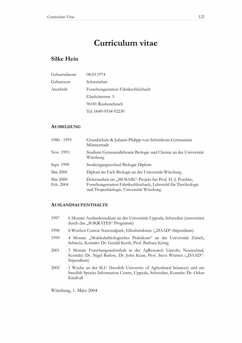
Curriculum Vitae 121
Curriculum vitae
Silke Hein
Geburtsdatum 08.03.1974
Geburtsort Schweinfurt
Anschrift Forschungsstation Fabrikschleichach
Glashüttenstr. 5
96181 Rauhenebrach
Tel. 0049-9554-92230
AUSBILDUNG
1980 - 1993 Grundschule & Johann-Philipp-von-Schönborn-Gymnasium Münnerstadt
Nov. 1993 Studium Gymnasiallehramt Biologie und Chemie an der Universität Würzburg
Sept. 1999 Studiengangwechsel Biologie Diplom
Mai 2000 Diplom im Fach Biologie an der Universität Würzburg
Mai 2000- Feb. 2004
Doktorarbeit im „MOSAIK“-Projekt bei Prof. H.-J. Poethke, Forschungsstation Fabrikschleichach, Lehrstuhl für Tierökologie und Tropenbiologie, Universität Würzburg
AUSLANDSAUFENTHALTE
1997 6 Monate Auslandsstudium an der Universität Uppsala, Schweden (unterstützt durch das „SOKRATES“ Programm)
1998 8 Wochen Comoé Nationalpark, Elfenbeinküste („DAAD“-Stipendium)
1999 4 Monate „Molekularbiologisches Praktikum“ an der Universität Zürich, Schweiz, Kontakt: Dr. Gerald Kerth, Prof. Barbara König
2001 3 Monate Forschungsaufenthalt in der AgResearch Lincoln, Neuseeland, Kontakt: Dr. Nigel Barlow, Dr. John Kean, Prof. Steve Wratten („DAAD“-Stipendium)
2002 1 Woche an der SLU (Swedish University of Agricultural Sciences) und am Swedish Species Information Centre, Uppsala, Schweden, Kontakt: Dr. Oskar Kindvall
Würzburg, 1. März 2004


123
Danksagung
Viele Menschen haben mich während dieser Arbeit unterstützt und mir
geholfen. Bei Ihnen allen möchte ich mich herzlich bedanken. Zunächst möchte ich mich bei Achim Poethke für das Vertrauen, das er
mir besonders zu Beginn und auch während der Arbeit entgegen gebracht hat, bedanken. Er hat mir immer den nötigen Freiraum für eine eigenständige Arbeit gelassen, war aber immer auch verfügbar, wenn ich Hilfe brauchte. Ich danke ihm für viele konstruktive Diskussionen und innovative Ideen. Er hat auch mein Interesse an der Modellierung geweckt und ich hoffe, ich kann dabei auch noch ein Weilchen bleiben.
Eine wichtige Rolle für mich und diese Arbeit spielte auch Thomas Hovestadt. Ohne seine Hilfe, sowohl theoretisch als auch bei der Formulierung unserer Veröffentlichungen, wären selbige wohl kaum zustande gekommen. Seine Gutmütigkeit, sowie die umfangreichen Statistikkenntnisse, ein ergiebiges Literaturwissen und eine immer währende Bereitschaft zur Diskussion trugen zum Gelingen dieser Arbeit und zu meiner Ausbildung bei. Gleichzeitig ist er dafür verantwortlich, dass ich neben der Doktorarbeit, nun auch ohne weiteres in die gehobene Küche einsteigen kann.
Jule Gombert, Julia Voss und Claudius Stanke haben während ihrer Diplomarbeiten dazu beigetragen, dass meine Freilandarbeiten lustig, unterhaltsam und nie langweilig wurden, dafür danke ich Ihnen herzlich. Sie haben die Zeit meiner Doktorarbeit an der Station angenehm bunt und heimelig werden lassen. Besonders glücklich bin ich, dass aus unserem „Dienstverhältnis“ wirklich tolle Freundschaften entstanden sind und ich hoffe das bleibt auch weiterhin so.
Die Forschungsstation Fabrikschleichach war für mich immer ein angenehmer Arbeitsplatz. Verantwortlich dafür sind die Menschen, die dort arbeiten. Ihnen allen danke ich herzlich. Besonders danke ich Brenda Pfenning für die tolle Zusammenarbeit und für die anstrengenden, aber auch lustigen Stunden, die wir für unser erstes gemeinsames Seminar miteinander verbracht haben. Jederzeit wieder!! Ihr und auch Elisabeth Obermeier danke ich weiterhin für ihre Freundschaft und Unterstützung in vielen Diskussionen.
Anne Böhm ist sicherlich die gute und perfekt organisierte „Seele“ der Station. Sie hatte immer ein gutes Wort und ein offenes Ohr, wenn es Probleme gab oder ich einfach nur mal quatschen wollte. Ihre Bonbongaben haben immer zur Aufheiterung beigetragen. Gleichzeitig war sie immer eine kompetente Hilfe beim Ausfüllen aller amtlichen Anfragen und Abrechnungen. Viele Deiner Hilfen gehen sicher weit über das hinaus was Dein „Job“ ist Anne, vielen, lieben Dank dafür. Roland Bickel lieferte alle praktischen Hilfsmittel, die für die Freilandarbeit nötig waren, in perfekter handwerklicher Ausführung. Hildegard Schramm war
124
immer verfügbar, wenn mir oder anderen an der Station ein Malheur (ob in der Küche oder auf der Heimfahrt) passiert war. Euch beiden: Vielen Dank!!
Für die Möglichkeit im Naturschutzgebiet „Hohe Wann“ mit Heuschrecken arbeiten zu können danke ich der Unteren und Oberen Naturschutzbehörde (Würzburg).
Diese Arbeit ist Teil des Verbundprojektes MOSAIK. Alle Kollegen trugen dazu bei, dass wir ein wirklich tolles Projektteam waren, so dass die Statusseminare für mich immer sehr schöne Erlebnisse waren. Ich empfand die Zusammenarbeit im Projekt als extrem zuträglich für meine Arbeit. Vor allem die Hilfe von Boris Schröder trug wesentlich zum Gelingen des Habitatmodellteils dieser Arbeit bei. Er war immer zu Diskussionen bereit und wurde nicht müde alles immer und immer wieder in „Konzeptvorstellungen“ zu besprechen. Ohne seine Hilfe wären die Habitatmodelle bei weitem nicht so weit gediehen.
Besonderer Dank gebührt auch Birgit Binzenhöfer. Ihr danke ich für ihr Durchhaltevermögen beim gemeinsamen Einrichten der Untersuchungsflächen. Weiterhin haben ihre umfassenden Freilandkenntnisse (sowohl zoologisch also auch botanisch) sowie auch die gemeinsamen Diskussionen zu den Habitatmodellen zur Verbesserung dieser Arbeit beigetragen.
Katrin Fritzsch danke ich für die lustige Zeit an der Station und bei Besuchen in Oldenburg, für unzählige CDs guter Musik und für viele interessante Gespräche.
Für die gute Zusammenarbeit bei der Freilandarbeit danke ich Helene Rümer, Caroline Rosenberger, Martina Wagner, Julia Mäschig, Corinna Pohl, Anja Teicher, Stefanie Döbler, Timo Pöhner wie auch Anna Eichner. Eckhard Gottschalk danke ich für die Exkursionen bei denen ich immer viel gelernt habe, und das nicht nur über Heuschrecken.
Die Freundschaft mit Kerstin Fröhle, Jule Gombert, Julia Voss, Claudius Stanke, Christian Herbert, Andree Thomas und Ralf Lohse (Lehrling) hat mir geholfen über der Doktorarbeit den „Rest“ nicht zu vergessen. Sie waren außerdem auch immer für mich da, wenn es mal nicht so lief.
Ich danke Lars Fieseler für die Geduld, wenn wieder einmal ein perfektes „Kletterwochenende“ zu einem „Freilandwochenende“ wurde und für die Zeit, die ich zusammen mit ihm verbringen kann, sowie für viele andere Dinge, die sich hier gar nicht aufzählen lassen.
Ganz besonderer Dank gilt meiner Familie. Meinen Geschwistern für ihre Freundschaft und Nähe, meinen Eltern sowohl für ihre finanzielle Unterstützung, als auch dafür, dass Sie mich bei all meinen Entscheidungen unterstützt haben und für ihre Tochter immer da sind.
Erklärung
gemäß § 4 Abs. 3 Ziff. 3, 5 und 8
der Promotionsordnung der Fakultät für Biologie der
Bayerischen Julius-Maximilians-Universität Würzburg
Hiermit erkläre ich ehrenwörtlich, die vorliegende Arbeit in allen Teilen selbständig und nur mit den angegebenen Quellen und Hilfsmitteln angefertigt zu haben. Diese Dissertation hat weder in gleicher noch in ähnlicher Form in einem anderen Prüfungsverfahren vorgelegen. Des weiteren erkläre ich, dass ich früher weder akademische Grade erworben habe, noch zu erwerben versucht habe.
Würburg, den 01.03.04 (Silke Hein)